ECE 8443 – Pattern RecognitionECE 8527 – Introduction to Machine Learning and Pattern Recognition

• Objectives:Cross-ValidationML and Bayesian Model ComparisonCombining Classifiers

• Resources:AM: Cross-ValidationCV: Bayesian Model AveragingVISP: Classifier Combination

LECTURE 24: COMBINING CLASSIFIERS

ECE 8527: Lecture 24, Slide 2

Learning With Queries• In previous sections, we assumed a set of labeled training patterns and

employed resampling methods to improve classification.

• When no labels are available, or the cost of generating truth-marked data is high, how can we decide what is the next best pattern(s) to be truth-marked and added to the training database?

• The solution to this problem goes by many names including active learning (maximizing the impact of each new data point) and cost-based learning (simultaneously minimizing classifier error rate and data collection cost).

• Two heuristic approaches to learning with queries: Confidence-based: select a data point for which the two largest discriminant

functions have nearly the same value. Voting-based: choose the pattern that yields the greatest disagreement

among the k component classifiers.

• Note that such approaches tend to ignore priors and attempt to focus on patterns near the decision boundary surface.

• The cost of collecting and truth-marking large amounts of data is almost always prohibitively high, and hence strategies to intelligently create training data are extremely important to any pattern recognition problem.

ECE 8527: Lecture 24, Slide 3

Cross-Validation• In simple validation, we randomly split the set of labeled training data into a

training set and a held-out set.

• The held-out set is used to estimate the generalization error.

• M-fold Cross-validation: The training set is divided into n/m disjoint sets, where n is the total number

of patterns and m is set heuristically. The classifier is trained m times, each time with a different held-out set as a

validation set. The estimated performance is the mean of these m error rates.

Such techniques can be applied to any learning algorithm. Key parameters, such as model size or complexity, can be optimized based on

the M-fold Cross-validation mean error rate. How much data should be held out? It depends on the application, but 80%

training / 10% development test set / 10% evaluation (or less) is not uncommon. Training sets are often too large to do M-fold Cross-validation.

Anti-cross-validation as also been used: adjusting parameters until the first local maximum is observed.

ECE 8527: Lecture 24, Slide 4

Jackknife and Bootstrap• Methods closely related to cross-validation are the jackknife and bootstrap

estimation procedures.

• Jackknife: train the classifier n separate times, each time deleting a single point. Test on the single deleted point. The jackknife estimate of the accuracy is the mean of these “leave-one-out” accuracies. Unfortunately, complexity is very high.

• Bootstrap: train B classifiers each with a different bootstrap data set, and test on the other bootstrap data sets. The bootstrap estimate of the classifier accuracy is the mean of these bootstrap accuracies.

ECE 8527: Lecture 24, Slide 5

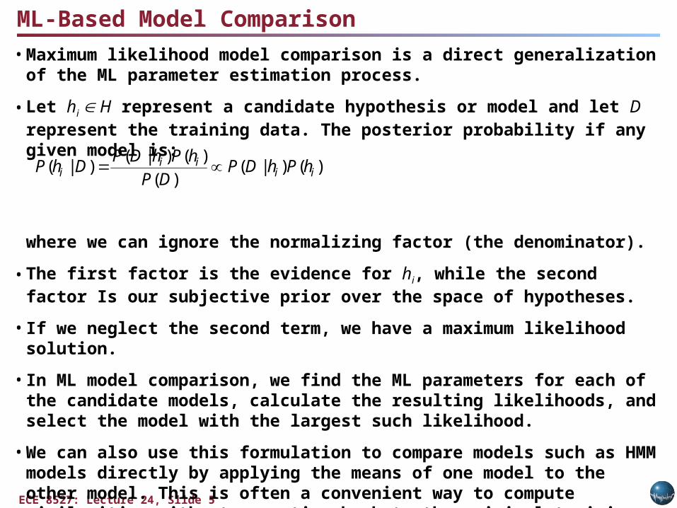
ML-Based Model Comparison• Maximum likelihood model comparison is a direct generalization of the ML

parameter estimation process.

• Let hi H represent a candidate hypothesis or model and let D represent the training data. The posterior probability if any given model is:

where we can ignore the normalizing factor (the denominator).

• The first factor is the evidence for hi, while the second factor Is our subjective prior over the space of hypotheses.

• If we neglect the second term, we have a maximum likelihood solution.

• In ML model comparison, we find the ML parameters for each of the candidate models, calculate the resulting likelihoods, and select the model with the largest such likelihood.

• We can also use this formulation to compare models such as HMM models directly by applying the means of one model to the other model. This is often a convenient way to compute similarities without reverting back to the original training data set.

)()|()(

)()|()|( iiii

i hPhDPDP

hPhDPDhP

ECE 8527: Lecture 24, Slide 6

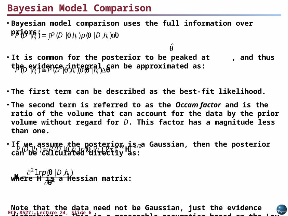
Bayesian Model Comparison• Bayesian model comparison uses the full information over priors:

• It is common for the posterior to be peaked at , and thus the evidence integral can be approximated as:

• The first term can be described as the best-fit likelihood.

• The second term is referred to as the Occam factor and is the ratio of the volume that can account for the data by the prior volume without regard for D. This factor has a magnitude less than one.

• If we assume the posterior is a Gaussian, then the posterior can be calculated directly as:

where H is a Hessian matrix:

Note that the data need not be Gaussian, just the evidence distribution. This is a reasonable assumption based on the Law of Large Numbers.

dhDphDPhDP iii ),|(),|()|(

θ )|ˆ(),ˆ|()|( iii hphDPhDP

2/12/)2)(|ˆ(),ˆ|()|( Hkiii hphDPhDP

2

2 ),|(lnθθH

ihDp

ECE 8527: Lecture 24, Slide 7

Combining Classifiers

),|(),|(),|( 0

1

00

0

k

rPrPP xyxxy

tk ],...,,[ 00

100

0

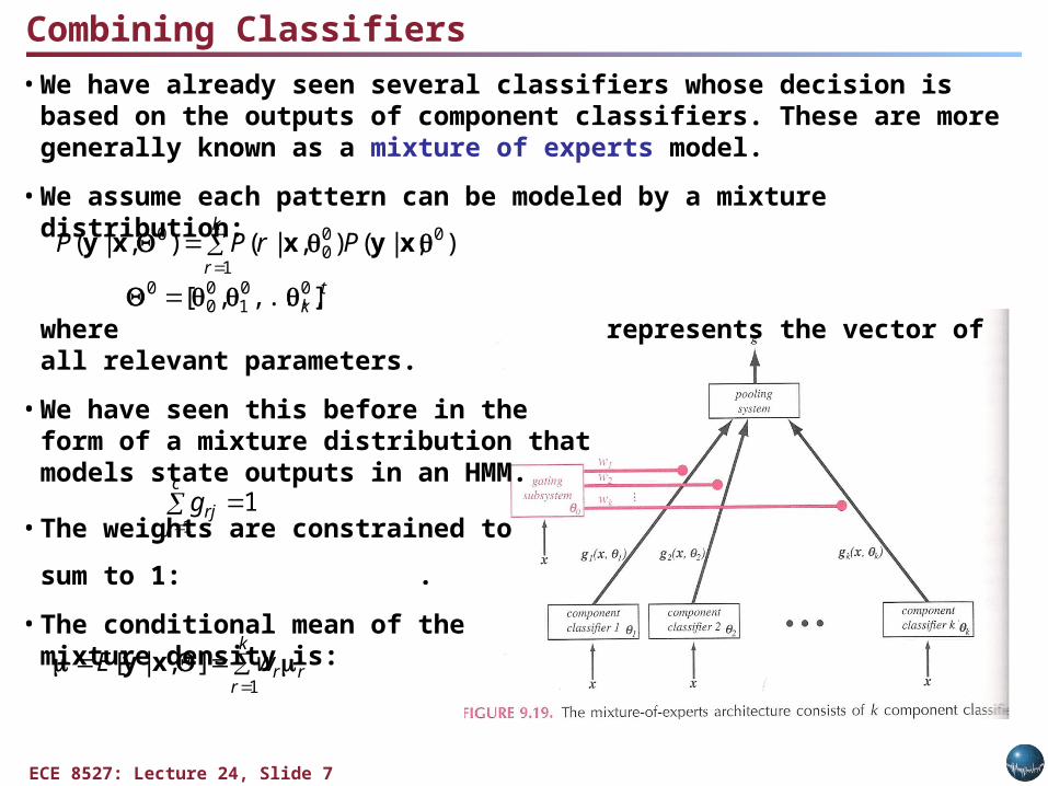
• We have already seen several classifiers whose decision is based on the outputs of component classifiers. These are more generally known as a mixture of experts model.

• We assume each pattern can be modeled by a mixture distribution:

where represents the vector of all relevant parameters.

• We have seen this before in the form of a mixture distribution thatmodels state outputs in an HMM.

• The weights are constrained to

sum to 1: .

• The conditional mean of themixture density is:

c

jrjg

11

k

rrrwE

1],|[ xy

ECE 8527: Lecture 24, Slide 8

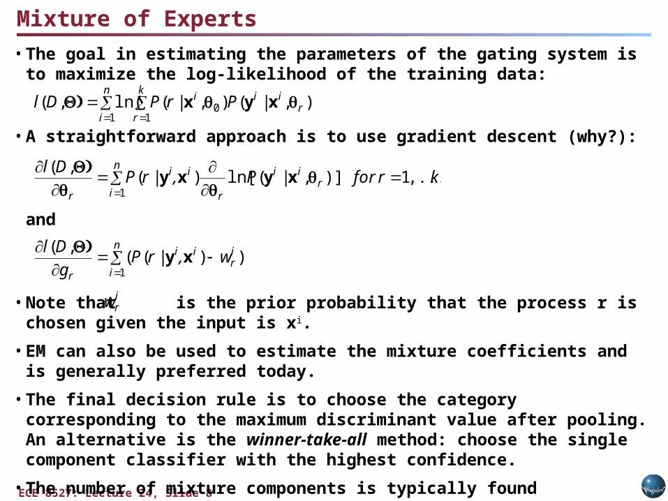
Mixture of Experts• The goal in estimating the parameters of the gating system is to maximize the

log-likelihood of the training data:

• A straightforward approach is to use gradient descent (why?):

and

• Note that is the prior probability that the process r is chosen given the input is xi.

• EM can also be used to estimate the mixture coefficients and is generally preferred today.

• The final decision rule is to choose the category corresponding to the maximum discriminant value after pooling. An alternative is the winner-take-all method: choose the single component classifier with the highest confidence.

• The number of mixture components is typically found experimentally.

krforP,rPDl n

ir

ii

r

ii

r,...,1)],|(ln[)|(,(

1

xyxy

n

i

k

rr

iii PrPDl1 1

0 )),|(),|(ln(,( xyx

n

i

ir

ii

rw,rP

gDl

1))|((,( xy

irw

ECE 8527: Lecture 24, Slide 9

Attributions• These slides were originally developed by R.S. Sutton and A.G. Barto,

Reinforcement Learning: An Introduction. (They have been reformatted and slightly annotated to better integrate them into this course.)

• The original slides have been incorporated into many machine learning courses, including Tim Oates’ Introduction of Machine Learning, which contains links to several good lectures on various topics in machine learning (and is where I first found these slides).

• A slightly more advanced version of the same material is available as part of Andrew Moore’s excellent set of statistical data mining tutorials.

• The objectives of this lecture are: describe the RL problem; present idealized form of the RL problem for which we have precise

theoretical results; introduce key components of the mathematics: value functions and Bellman

equations; describe trade-offs between applicability and mathematical tractability.

ECE 8527: Lecture 24, Slide 10

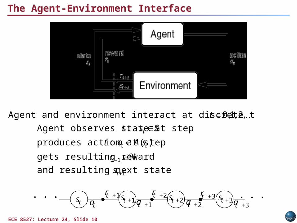
Agent and environment interact at discrete time steps: t 0,1, 2, Agent observes state at step t : st S produces action at step t : at A(st ) gets resulting reward: rt1 and resulting next state: st1

t. . . st a

rt +1 st +1t +1a

rt +2 st +2t +2a

rt +3 st +3. . .

t +3a

The Agent-Environment Interface

ECE 8527: Lecture 24, Slide 11

The Agent Learns A Policy• Definition of a policy:

Policy at state t, t , is a mapping from states to action probabilities.

t (s,a) = probability that at = a when st = s.

• Reinforcement learning methods specify how the agent changes its policy as a result of experience.

• Roughly, the agent’s goal is to get as much reward as it can over the long run.

• Learning can occur in several ways: Adaptation of classifier parameters based on prior and current data

(e.g., many help systems now ask you “was this answer helpful to you”).

Selection of the most appropriate next training pattern during classifier training (e.g., active learning).

• Common algorithm design issues include rate of convergence, bias vs. variance, adaptation speed, and batch vs. incremental adaptation.

ECE 8527: Lecture 24, Slide 12

• Time steps need not refer to fixed intervals of real time (e.g., each new training pattern can be considered a time step).

• Actions can be low level (e.g., voltages to motors), or high level (e.g., accept a job offer), “mental” (e.g., shift in focus of attention), etc. Actions can be rule-based (e.g., user expresses a preference) or mathematics-based (e.g., assignment of a class or update of a probability).

• States can be low-level “sensations”, or they can be abstract, symbolic, based on memory, or subjective (e.g., the state of being “surprised” or “lost”).

• States can be hidden or observable.• A reinforcement learning (RL) agent is not like a whole animal or robot, which

consist of many RL agents as well as other components.• The environment is not necessarily unknown to the agent, only incompletely

controllable.• Reward computation is in the agent’s environment because the agent cannot

change it arbitrarily.

Getting the Degree of Abstraction Right

ECE 8527: Lecture 24, Slide 13

• Is a scalar reward signal an adequate notion of a goal? Perhaps not, but it is surprisingly flexible.

• A goal should specify what we want to achieve, not how we want to achieve it.• A goal must be outside the agent’s direct control — thus outside the agent.• The agent must be able to measure success: explicitly frequently during its lifespan.

Goals

ECE 8527: Lecture 24, Slide 14

Returns• Suppose the sequence of rewards after step t is rt+1, rt+2,… What do we want to

maximize?

• In general, we want to maximize the expected return, E[Rt], for each step t, where Rt = rt+1 + rt+2 + … + rT, where T is a final time step at which a terminal state is reached, ending an episode. (You can view this as a variant of the forward backward calculation in HMMs.)

• Here episodic tasks denote a complete transaction (e.g., a play of a game, a trip through a maze, a phone call to a support line).

• Some tasks do not have a natural episode and can be considered continuing tasks. For these tasks, we can define the return as:

where is the discounting rate and 0 1. close to zero favors short-term returns (shortsighted) while close to 1 favors long-term returns. can also be thought of as a “forgetting factor” in that, since it is less than one, it weights near-term future actions more heavily than longer-term future actions.

013

221 ...

kkt

ktttt rrrrR

ECE 8527: Lecture 24, Slide 15

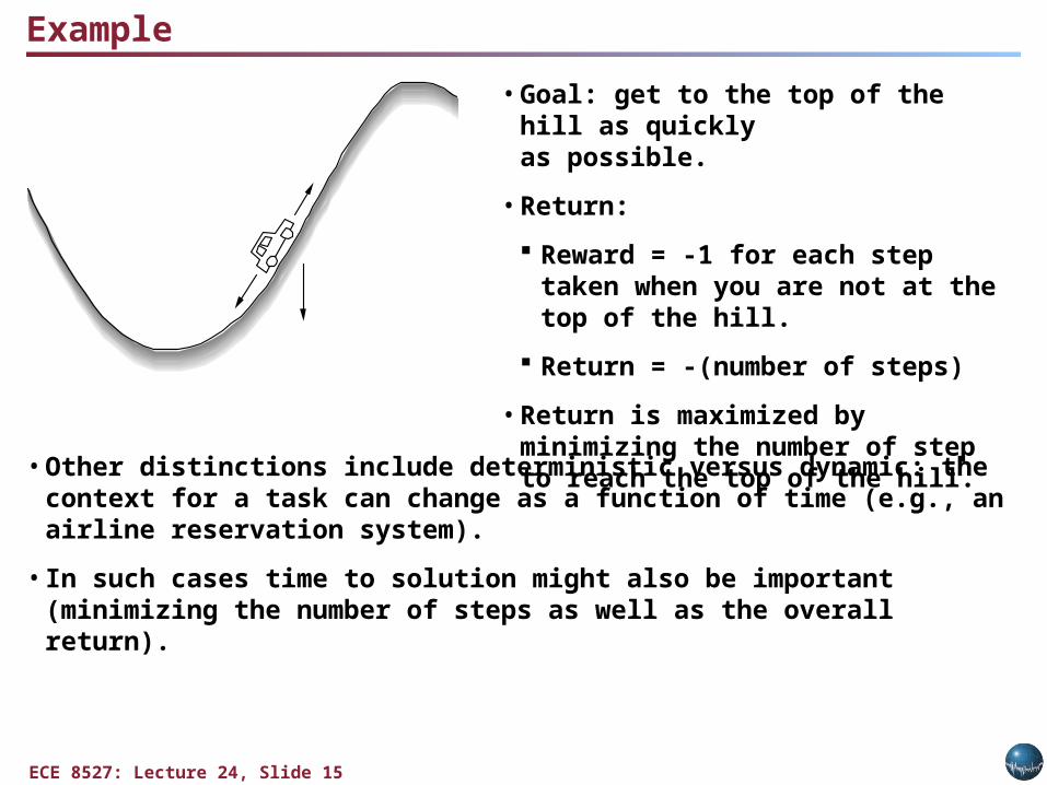
• Goal: get to the top of the hill as quicklyas possible.

• Return: Reward = -1 for each step taken when

you are not at the top of the hill. Return = -(number of steps)

• Return is maximized by minimizing the number of step to reach the top of the hill.

Example

• Other distinctions include deterministic versus dynamic: the context for a task can change as a function of time (e.g., an airline reservation system).

• In such cases time to solution might also be important (minimizing the number of steps as well as the overall return).

ECE 8527: Lecture 24, Slide 16

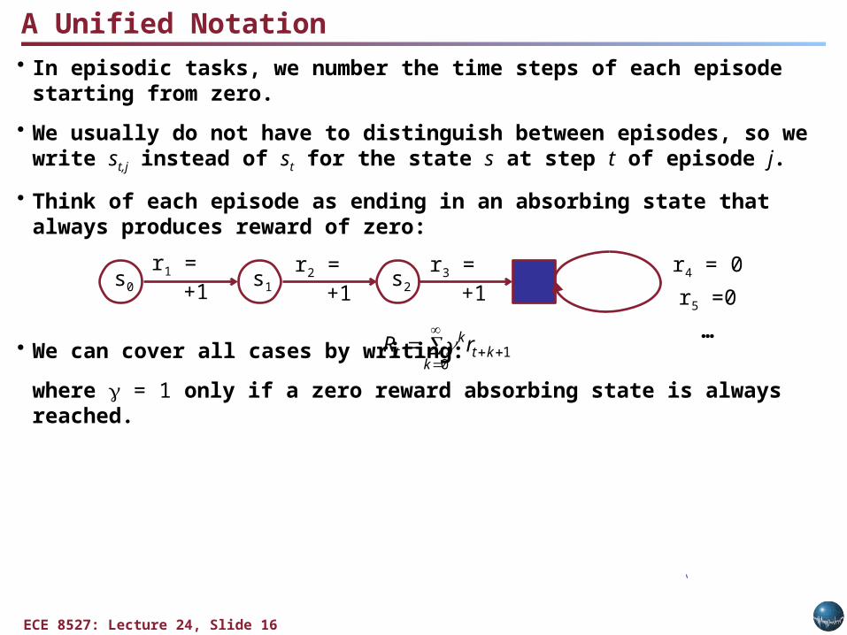
• In episodic tasks, we number the time steps of each episode starting from zero.

• We usually do not have to distinguish between episodes, so we write st,j instead of st for the state s at step t of episode j.

• Think of each episode as ending in an absorbing state that always produces reward of zero:

• We can cover all cases by writing:

where = 1 only if a zero reward absorbing state is always reached.

A Unified Notation

s0 s1 s2

r1 = +1 r2 = +1 r3 = +1 r4 = 0r5 =0…

01

kkt

kt rR

ECE 8527: Lecture 24, Slide 17

Summary• Introduced several approaches to improving classifier performance: Learning from Queries: select the most informative new training pattern so

that accuracy and cost can be simultaneously optimized.• Introduced new ways to estimate accuracy and generalization: M-Fold Cross-validation: estimating the error rate as the mean across

various subsets of the data. Jackknife and Bootstrap: alternate ways to repartition the training data to

estimate error rates.• Model comparison using maximum likelihood and Bayesian approaches.• Classifier combination using mixture of experts.• Agent-environment interaction (states, actions, rewards)• Policy: stochastic rule for selecting actions• Return: the function of future rewards agent tries to maximize• Episodic and continuing tasks