nutrient criteria manual estuarine coastal
TRANSCRIPT

United StatesEnvironmental Protection Agency
Office of Water4304
EPA-822-B-01-003October 2001
Nutrient CriteriaTechnical Guidance Manual
Estuarine and CoastalMarine Waters

U.S. Environmental Protection Agency
Nutrient CriteriaTechnical Guidance Manual
Estuarine and Coastal Marine Waters
October 2001

ii Nutrient Criteria—Estuarine and Coastal Waters
Disclaimer
This manual provides technical guidance to States, Indian Tribes, and other authorized jurisdictions toestablish water quality criteria and standards under the Clean Water Act (CWA), to protect aquatic lifefrom acute and chronic effects of nutrient overenrichment. Under the CWA, States and Indian Tribes areto establish water quality criteria to protect designated uses. State and Indian Tribal decisionmakersretain the discretion to adopt approaches on a case-by-case basis that differ from this guidance whenappropriate and scientifically defensible. Although this manual constitutes EPA's scientificrecommendations regarding ambient concentrations of nutrients that protect resource quality and aquaticlife, it does not substitute for the CWA or EPA's regulations; nor is it a regulation itself. Thus, it cannotimpose legally binding requirements on EPA, States, Indian Tribes, or the regulated community, andmight not apply to a particular situation or circumstance. EPA may change this guidance in the future.
Cover Photograph: Somewhere on the Chesapeake Bay. Supplied by David Flemer as a duplicate copyfrom the Chesapeake Biological Laboratory Photo Archives, University of Maryland; date unknown butearlier than 1972.

iiiNutrient Criteria—Estuarine and Coastal Waters
CONTENTS
Contributors . . . . . . . . . . . . . . . . . . . . . . . . . . . . . . . . . . . . . . . . . . . . . . . . . . . . . . . . . . . . . . . . . . . . . . . . xiAcknowledgments . . . . . . . . . . . . . . . . . . . . . . . . . . . . . . . . . . . . . . . . . . . . . . . . . . . . . . . . . . . . . . . . . . xiiiForeword . . . . . . . . . . . . . . . . . . . . . . . . . . . . . . . . . . . . . . . . . . . . . . . . . . . . . . . . . . . . . . . . . . . . . . . . . xvExecutive Summary . . . . . . . . . . . . . . . . . . . . . . . . . . . . . . . . . . . . . . . . . . . . . . . . . . . . . . . . . . . . . . . . xvii
Chapter 1. Introduction and Objectives . . . . . . . . . . . . . . . . . . . . . . . . . . . . . . . . . . . . . . . . . . . . . . . 1-1
1.1 Backround . . . . . . . . . . . . . . . . . . . . . . . . . . . . . . . . . . . . . . . . . . . . . . . . . . . . . . . . . . . . . . . . . . . . . 1-11.2 Definition of Estuaries and Coastal Systems . . . . . . . . . . . . . . . . . . . . . . . . . . . . . . . . . . . . . . . . . . 1-21.3 Nature of the Nutrient Overenrichment Problem in Estuarine and Coastal Marine Waters . . . . . . 1-5
Scope and Magnitude of the Problem . . . . . . . . . . . . . . . . . . . . . . . . . . . . . . . . . . . . . . . . . . . . . . . 1-51.4 The Nutrient Criteria Development Process . . . . . . . . . . . . . . . . . . . . . . . . . . . . . . . . . . . . . . . . . . . 1-8
Preliminary Steps . . . . . . . . . . . . . . . . . . . . . . . . . . . . . . . . . . . . . . . . . . . . . . . . . . . . . . . . . . . . . . 1-8Strategy for Reducing Human-Based Eutrophication . . . . . . . . . . . . . . . . . . . . . . . . . . . . . . . . . 1-10Nutrient Criteria Development Process . . . . . . . . . . . . . . . . . . . . . . . . . . . . . . . . . . . . . . . . . . . . 1-11
Chapter 2. Scientific Basis for Estuarine and Coastal Waters Quantitative Nutrient Criteria . . 2-1
2.1 Introduction . . . . . . . . . . . . . . . . . . . . . . . . . . . . . . . . . . . . . . . . . . . . . . . . . . . . . . . . . . . . . . . . . . . . 2-1Purpose and Overview . . . . . . . . . . . . . . . . . . . . . . . . . . . . . . . . . . . . . . . . . . . . . . . . . . . . . . . . . . 2-1Some Important Nutrient-Related Scientific Issues . . . . . . . . . . . . . . . . . . . . . . . . . . . . . . . . . . . . 2-2River-to-Ocean Continuum: Watershed/Nearshore Coastal Management Framework . . . . . . . . . 2-5
2.2 Controlling the Right Nutrients . . . . . . . . . . . . . . . . . . . . . . . . . . . . . . . . . . . . . . . . . . . . . . . . . . . 2-10Overview . . . . . . . . . . . . . . . . . . . . . . . . . . . . . . . . . . . . . . . . . . . . . . . . . . . . . . . . . . . . . . . . . . . . 2-10Some Empirical Evidence for N Limitation of Net Primary Production . . . . . . . . . . . . . . . . . . . 2-11Some Threshold Responses to Nitrogen Overenrichment . . . . . . . . . . . . . . . . . . . . . . . . . . . . . . 2-13Effects of Physical Forcing on Net Primary Production . . . . . . . . . . . . . . . . . . . . . . . . . . . . . . . 2-13Other Physical Factors . . . . . . . . . . . . . . . . . . . . . . . . . . . . . . . . . . . . . . . . . . . . . . . . . . . . . . . . . 2-23
2.3 Nutrient Loads and Concentrations: Interpretation of Effects . . . . . . . . . . . . . . . . . . . . . . . . . . . . 2-21Conceptual Framework . . . . . . . . . . . . . . . . . . . . . . . . . . . . . . . . . . . . . . . . . . . . . . . . . . . . . . . . . 2-24Examples . . . . . . . . . . . . . . . . . . . . . . . . . . . . . . . . . . . . . . . . . . . . . . . . . . . . . . . . . . . . . . . . . . . . 2-24
2.4 Physical-Chemical Processes and Dissolved Oxygen Deficiency . . . . . . . . . . . . . . . . . . . . . . . . . 2-272.5 Nutrient Overenrichment Effects and Important Biological Resources . . . . . . . . . . . . . . . . . . . . 2-28
Benthic Vascular Plant Responses to Nutrients . . . . . . . . . . . . . . . . . . . . . . . . . . . . . . . . . . . . . . 2-28Other Examples of Important Biotic Effects of Nutrient Overenrichment . . . . . . . . . . . . . . . . . . 2-29
2.6 Concluding Statement on Nitrogen and Phosphorus Controls . . . . . . . . . . . . . . . . . . . . . . . . . . . . 2-32
Chapter 3. Classification of Estuarine and Coastal Waters . . . . . . . . . . . . . . . . . . . . . . . . . . . . . . . 3-1
3.1 Introduction . . . . . . . . . . . . . . . . . . . . . . . . . . . . . . . . . . . . . . . . . . . . . . . . . . . . . . . . . . . . . . . . . . . . 3-1Purpose and Background . . . . . . . . . . . . . . . . . . . . . . . . . . . . . . . . . . . . . . . . . . . . . . . . . . . . . . . . 3-1Defining the Resource of Concern . . . . . . . . . . . . . . . . . . . . . . . . . . . . . . . . . . . . . . . . . . . . . . . . . 3-2
3.2 Major Factors Influencing Estuarine Susceptibility to Nutrient Overenrichment . . . . . . . . . . . . . . 3-2Dilution . . . . . . . . . . . . . . . . . . . . . . . . . . . . . . . . . . . . . . . . . . . . . . . . . . . . . . . . . . . . . . . . . . . . . . 3-3Water Residence Time . . . . . . . . . . . . . . . . . . . . . . . . . . . . . . . . . . . . . . . . . . . . . . . . . . . . . . . . . . 3-3Stratification . . . . . . . . . . . . . . . . . . . . . . . . . . . . . . . . . . . . . . . . . . . . . . . . . . . . . . . . . . . . . . . . . . 3-3

CONTENTS (continued)
iv Nutrient Criteria—Estuarine and Coastal Waters
3.3 Examples of Coastal Classification . . . . . . . . . . . . . . . . . . . . . . . . . . . . . . . . . . . . . . . . . . . . . . . . . 3-4Geomorphic Classification . . . . . . . . . . . . . . . . . . . . . . . . . . . . . . . . . . . . . . . . . . . . . . . . . . . . . . . 3-4Man-Made Estuaries . . . . . . . . . . . . . . . . . . . . . . . . . . . . . . . . . . . . . . . . . . . . . . . . . . . . . . . . . . . . 3-6Physical/Hydrodynamic Factor–Based Classifications . . . . . . . . . . . . . . . . . . . . . . . . . . . . . . . . . 3-6Other Considerations . . . . . . . . . . . . . . . . . . . . . . . . . . . . . . . . . . . . . . . . . . . . . . . . . . . . . . . . . . . 3-9Summary . . . . . . . . . . . . . . . . . . . . . . . . . . . . . . . . . . . . . . . . . . . . . . . . . . . . . . . . . . . . . . . . . . . . 3-11
3.4 Coastal Waters Seaward of Estuaries . . . . . . . . . . . . . . . . . . . . . . . . . . . . . . . . . . . . . . . . . . . . . . . 3-11Geomorphic Classification . . . . . . . . . . . . . . . . . . . . . . . . . . . . . . . . . . . . . . . . . . . . . . . . . . . . . . 3-12Nongeomorphic Classification . . . . . . . . . . . . . . . . . . . . . . . . . . . . . . . . . . . . . . . . . . . . . . . . . . . 3-13
Chapter 4. Variables and Measurement Methods To Assess and MonitorEstuarine/Marine Eutrophic Conditions . . . . . . . . . . . . . . . . . . . . . . . . . . . . . . . . . . . . . . . . . . 4-1
4.1 Introduction . . . . . . . . . . . . . . . . . . . . . . . . . . . . . . . . . . . . . . . . . . . . . . . . . . . . . . . . . . . . . . . . . . . . 4-14.2 Causal and Response Indicator Variables . . . . . . . . . . . . . . . . . . . . . . . . . . . . . . . . . . . . . . . . . . . . . 4-2
Nutrients as Causal Variables . . . . . . . . . . . . . . . . . . . . . . . . . . . . . . . . . . . . . . . . . . . . . . . . . . . . . 4-2Response Variables . . . . . . . . . . . . . . . . . . . . . . . . . . . . . . . . . . . . . . . . . . . . . . . . . . . . . . . . . . . . . 4-6Measures of Water Clarity . . . . . . . . . . . . . . . . . . . . . . . . . . . . . . . . . . . . . . . . . . . . . . . . . . . . . . . 4-7Dissolved Oxygen . . . . . . . . . . . . . . . . . . . . . . . . . . . . . . . . . . . . . . . . . . . . . . . . . . . . . . . . . . . . . . 4-8Benthic Macroinfauna . . . . . . . . . . . . . . . . . . . . . . . . . . . . . . . . . . . . . . . . . . . . . . . . . . . . . . . . . . 4-9
4.3 Field Sampling and Laboratory Analytical Methods . . . . . . . . . . . . . . . . . . . . . . . . . . . . . . . . . . . . . 4-9Field Sampling Methods . . . . . . . . . . . . . . . . . . . . . . . . . . . . . . . . . . . . . . . . . . . . . . . . . . . . . . . . . 4-9Laboratory Analytical Methods . . . . . . . . . . . . . . . . . . . . . . . . . . . . . . . . . . . . . . . . . . . . . . . . . . 4-13Water Column Nutrients . . . . . . . . . . . . . . . . . . . . . . . . . . . . . . . . . . . . . . . . . . . . . . . . . . . . . . . . 4-13Sediment Analyses . . . . . . . . . . . . . . . . . . . . . . . . . . . . . . . . . . . . . . . . . . . . . . . . . . . . . . . . . . . . 4-15Determination of Primary Productivity . . . . . . . . . . . . . . . . . . . . . . . . . . . . . . . . . . . . . . . . . . . . 4-16Phytoplankton Species Composition . . . . . . . . . . . . . . . . . . . . . . . . . . . . . . . . . . . . . . . . . . . . . . 4-16Macrobenthos, Macroalgae, and Seagrasses and SAV . . . . . . . . . . . . . . . . . . . . . . . . . . . . . . . . . 4-17
Chapter 5. Databases, Sampling Design, and Data Analysis . . . . . . . . . . . . . . . . . . . . . . . . . . . . . . 5-1
5.1 Introduction . . . . . . . . . . . . . . . . . . . . . . . . . . . . . . . . . . . . . . . . . . . . . . . . . . . . . . . . . . . . . . . . . . . . 5-15.2 Developing Regional and National Databases for Estuaries and Coastal Waters . . . . . . . . . . . . . . 5-1
Data Sources . . . . . . . . . . . . . . . . . . . . . . . . . . . . . . . . . . . . . . . . . . . . . . . . . . . . . . . . . . . . . . . . . . 5-3EPA Water Quality Data . . . . . . . . . . . . . . . . . . . . . . . . . . . . . . . . . . . . . . . . . . . . . . . . . . . . . . . . 5-3National Oceanographic and Atmospheric Administration (NOAA) . . . . . . . . . . . . . . . . . . . . . . 5-5Rivers and Streams Water Quality Data . . . . . . . . . . . . . . . . . . . . . . . . . . . . . . . . . . . . . . . . . . . . . 5-6USGS San Francisco Bay Program . . . . . . . . . . . . . . . . . . . . . . . . . . . . . . . . . . . . . . . . . . . . . . . . . 5-6State/Tribal Monitoring Programs . . . . . . . . . . . . . . . . . . . . . . . . . . . . . . . . . . . . . . . . . . . . . . . . . 5-7Sanitation Districts . . . . . . . . . . . . . . . . . . . . . . . . . . . . . . . . . . . . . . . . . . . . . . . . . . . . . . . . . . . . . 5-7Academic and Literature Sources . . . . . . . . . . . . . . . . . . . . . . . . . . . . . . . . . . . . . . . . . . . . . . . . . . 5-8Volunteer Monitoring Programs . . . . . . . . . . . . . . . . . . . . . . . . . . . . . . . . . . . . . . . . . . . . . . . . . . . 5-8Quality of Historical Data . . . . . . . . . . . . . . . . . . . . . . . . . . . . . . . . . . . . . . . . . . . . . . . . . . . . . . . . 5-9Location Data . . . . . . . . . . . . . . . . . . . . . . . . . . . . . . . . . . . . . . . . . . . . . . . . . . . . . . . . . . . . . . . . . 5-9Variables and Analytical Methods . . . . . . . . . . . . . . . . . . . . . . . . . . . . . . . . . . . . . . . . . . . . . . . . . 5-9Laboratory Quality Control . . . . . . . . . . . . . . . . . . . . . . . . . . . . . . . . . . . . . . . . . . . . . . . . . . . . . . 5-9Data Collecting Agencies . . . . . . . . . . . . . . . . . . . . . . . . . . . . . . . . . . . . . . . . . . . . . . . . . . . . . . . 5-10Time Period . . . . . . . . . . . . . . . . . . . . . . . . . . . . . . . . . . . . . . . . . . . . . . . . . . . . . . . . . . . . . . . . . 5-10

CONTENTS (continued)
vNutrient Criteria—Estuarine and Coastal Waters
Index Period . . . . . . . . . . . . . . . . . . . . . . . . . . . . . . . . . . . . . . . . . . . . . . . . . . . . . . . . . . . . . . . . . 5-10Representativeness . . . . . . . . . . . . . . . . . . . . . . . . . . . . . . . . . . . . . . . . . . . . . . . . . . . . . . . . . . . . 5-10Gathering New Data . . . . . . . . . . . . . . . . . . . . . . . . . . . . . . . . . . . . . . . . . . . . . . . . . . . . . . . . . . . 5-10
5.3 Sampling Design . . . . . . . . . . . . . . . . . . . . . . . . . . . . . . . . . . . . . . . . . . . . . . . . . . . . . . . . . . . . . . . 5-10Sampling Protocol . . . . . . . . . . . . . . . . . . . . . . . . . . . . . . . . . . . . . . . . . . . . . . . . . . . . . . . . . . . . . 5-11Sampling Technique . . . . . . . . . . . . . . . . . . . . . . . . . . . . . . . . . . . . . . . . . . . . . . . . . . . . . . . . . . . 5-12Initial Considerations . . . . . . . . . . . . . . . . . . . . . . . . . . . . . . . . . . . . . . . . . . . . . . . . . . . . . . . . . . 5-12Specifying the Population and Sample Unit . . . . . . . . . . . . . . . . . . . . . . . . . . . . . . . . . . . . . . . . . 5-13Specifying the Reporting Unit . . . . . . . . . . . . . . . . . . . . . . . . . . . . . . . . . . . . . . . . . . . . . . . . . . . 5-14Sources of Variability . . . . . . . . . . . . . . . . . . . . . . . . . . . . . . . . . . . . . . . . . . . . . . . . . . . . . . . . . . 5-14Alternative Sampling Designs . . . . . . . . . . . . . . . . . . . . . . . . . . . . . . . . . . . . . . . . . . . . . . . . . . . 5-16Monitoring Programs . . . . . . . . . . . . . . . . . . . . . . . . . . . . . . . . . . . . . . . . . . . . . . . . . . . . . . . . . . 5-18Citizen Monitoring Programs . . . . . . . . . . . . . . . . . . . . . . . . . . . . . . . . . . . . . . . . . . . . . . . . . . . . 5-20
5.4 Quality Assurance/Quality Control . . . . . . . . . . . . . . . . . . . . . . . . . . . . . . . . . . . . . . . . . . . . . . . . 5-21Representativeness . . . . . . . . . . . . . . . . . . . . . . . . . . . . . . . . . . . . . . . . . . . . . . . . . . . . . . . . . . . . 5-21Completeness . . . . . . . . . . . . . . . . . . . . . . . . . . . . . . . . . . . . . . . . . . . . . . . . . . . . . . . . . . . . . . . . 5-21Comparability . . . . . . . . . . . . . . . . . . . . . . . . . . . . . . . . . . . . . . . . . . . . . . . . . . . . . . . . . . . . . . . . 5-21Accuracy . . . . . . . . . . . . . . . . . . . . . . . . . . . . . . . . . . . . . . . . . . . . . . . . . . . . . . . . . . . . . . . . . . . . 5-22Variability . . . . . . . . . . . . . . . . . . . . . . . . . . . . . . . . . . . . . . . . . . . . . . . . . . . . . . . . . . . . . . . . . . . 5-22
5.5 Statistical Analyses . . . . . . . . . . . . . . . . . . . . . . . . . . . . . . . . . . . . . . . . . . . . . . . . . . . . . . . . . . . . . 5-22Data Reduction . . . . . . . . . . . . . . . . . . . . . . . . . . . . . . . . . . . . . . . . . . . . . . . . . . . . . . . . . . . . . . . 5-22Frequency Distributions . . . . . . . . . . . . . . . . . . . . . . . . . . . . . . . . . . . . . . . . . . . . . . . . . . . . . . . . 5-23Correlation and Regression Analyses . . . . . . . . . . . . . . . . . . . . . . . . . . . . . . . . . . . . . . . . . . . . . 5-23Tests of Significance . . . . . . . . . . . . . . . . . . . . . . . . . . . . . . . . . . . . . . . . . . . . . . . . . . . . . . . . . . 5-24
Chapter 6. Determining the Reference Condition . . . . . . . . . . . . . . . . . . . . . . . . . . . . . . . . . . . . . . . 6-1
6.1 Introduction and Definition . . . . . . . . . . . . . . . . . . . . . . . . . . . . . . . . . . . . . . . . . . . . . . . . . . . . . . . 6-16.2 Significance of Reference Conditions . . . . . . . . . . . . . . . . . . . . . . . . . . . . . . . . . . . . . . . . . . . . . . . 6-16.3 Paucity of Similar Estuarine and Coastal Marine Ecosystems . . . . . . . . . . . . . . . . . . . . . . . . . . . . . 6-46.4 Approaches for Establishing Reference Conditions . . . . . . . . . . . . . . . . . . . . . . . . . . . . . . . . . . . . . 6-4
In Situ Observations as the Basis for Estuarine Reference Condition . . . . . . . . . . . . . . . . . . . . . . 6-5Areal Load Approach to Identification of Reference Condition . . . . . . . . . . . . . . . . . . . . . . . . . 6-11
Chapter 7. Nutrient and Algal Criteria Development . . . . . . . . . . . . . . . . . . . . . . . . . . . . . . . . . . . . 7-1
7.1 Introduction . . . . . . . . . . . . . . . . . . . . . . . . . . . . . . . . . . . . . . . . . . . . . . . . . . . . . . . . . . . . . . . . . . . . 7-17.2 Role of Regional Technical Assistance Groups . . . . . . . . . . . . . . . . . . . . . . . . . . . . . . . . . . . . . . . . 7-27.3 Classification . . . . . . . . . . . . . . . . . . . . . . . . . . . . . . . . . . . . . . . . . . . . . . . . . . . . . . . . . . . . . . . . . . 7-37.4 Descriptive Background Information . . . . . . . . . . . . . . . . . . . . . . . . . . . . . . . . . . . . . . . . . . . . . . . . 7-3
Estuarine Watershed Characterization . . . . . . . . . . . . . . . . . . . . . . . . . . . . . . . . . . . . . . . . . . . . . . 7-3Within Estuarine System Characterization . . . . . . . . . . . . . . . . . . . . . . . . . . . . . . . . . . . . . . . . . . . 7-4
7.5 Elements of Nutrient Criteria . . . . . . . . . . . . . . . . . . . . . . . . . . . . . . . . . . . . . . . . . . . . . . . . . . . . . . 7-5Reference Condition . . . . . . . . . . . . . . . . . . . . . . . . . . . . . . . . . . . . . . . . . . . . . . . . . . . . . . . . . . . . 7-5Historical Information . . . . . . . . . . . . . . . . . . . . . . . . . . . . . . . . . . . . . . . . . . . . . . . . . . . . . . . . . . 7-5Models . . . . . . . . . . . . . . . . . . . . . . . . . . . . . . . . . . . . . . . . . . . . . . . . . . . . . . . . . . . . . . . . . . . . . . 7-5Antidegradation Policy and Attention to Downstream Effects . . . . . . . . . . . . . . . . . . . . . . . . . . . 7-6The RTAG . . . . . . . . . . . . . . . . . . . . . . . . . . . . . . . . . . . . . . . . . . . . . . . . . . . . . . . . . . . . . . . . . . . 7-7

CONTENTS (continued)
vi Nutrient Criteria—Estuarine and Coastal Waters
7.6 Hypothetical Examples of Nutrient Criteria Development Deliberations . . . . . . . . . . . . . . . . . . . . 7-7Scenario . . . . . . . . . . . . . . . . . . . . . . . . . . . . . . . . . . . . . . . . . . . . . . . . . . . . . . . . . . . . . . . . . . . . . 7-7
7.7 Evaluation of Proposed Criteria . . . . . . . . . . . . . . . . . . . . . . . . . . . . . . . . . . . . . . . . . . . . . . . . . . . . 7-8Guidance for Interpreting and Applying Criteria . . . . . . . . . . . . . . . . . . . . . . . . . . . . . . . . . . . . . . 7-9Do the Criteria Protect Designated Uses? . . . . . . . . . . . . . . . . . . . . . . . . . . . . . . . . . . . . . . . . . . . 7-9Restoration Goals . . . . . . . . . . . . . . . . . . . . . . . . . . . . . . . . . . . . . . . . . . . . . . . . . . . . . . . . . . . . . 7-11Sampling for Comparison to Criteria . . . . . . . . . . . . . . . . . . . . . . . . . . . . . . . . . . . . . . . . . . . 7-11
7.8 Nutrient Criteria Interpretation Procedures . . . . . . . . . . . . . . . . . . . . . . . . . . . . . . . . . . . . . . . . . . 7-12Decisionmaking Protocol . . . . . . . . . . . . . . . . . . . . . . . . . . . . . . . . . . . . . . . . . . . . . . . . . . . . . . . 7-12Multivariable Enrichment Index . . . . . . . . . . . . . . . . . . . . . . . . . . . . . . . . . . . . . . . . . . . . . . . . . . 7-12Frequency and Duration . . . . . . . . . . . . . . . . . . . . . . . . . . . . . . . . . . . . . . . . . . . . . . . . . . . . . . . . 7-13
7.9 Criteria Modifications . . . . . . . . . . . . . . . . . . . . . . . . . . . . . . . . . . . . . . . . . . . . . . . . . . . . . . . . . . . 7-147.10 EPA, State, or Tribe Responsibility under the Clean Water Act . . . . . . . . . . . . . . . . . . . . . . . . . 7-147.11 Implementation of Nutrient Criteria into Water Quality Standards . . . . . . . . . . . . . . . . . . . . . . . 7-14
Chapter 8. Using Nutrient Criteria to Protect Water Quality . . . . . . . . . . . . . . . . . . . . . . . . . . . . . 8-1
8.1 Managing Point Source Pollution . . . . . . . . . . . . . . . . . . . . . . . . . . . . . . . . . . . . . . . . . . . . . . . . . . . 8-1The Clean Water Act and Water Quality Standards . . . . . . . . . . . . . . . . . . . . . . . . . . . . . . . . . . . . 8-1Protecting Designated Uses . . . . . . . . . . . . . . . . . . . . . . . . . . . . . . . . . . . . . . . . . . . . . . . . . . . . . . 8-2Maintaining Existing Water Quality . . . . . . . . . . . . . . . . . . . . . . . . . . . . . . . . . . . . . . . . . . . . . . . . 8-3General Policies . . . . . . . . . . . . . . . . . . . . . . . . . . . . . . . . . . . . . . . . . . . . . . . . . . . . . . . . . . . . . . . 8-4Providing Flexibility in Implementation . . . . . . . . . . . . . . . . . . . . . . . . . . . . . . . . . . . . . . . . . . . . . 8-6NPDES Permits . . . . . . . . . . . . . . . . . . . . . . . . . . . . . . . . . . . . . . . . . . . . . . . . . . . . . . . . . . . . . . . . 8-7Look to the Future ... Pollutant Trading . . . . . . . . . . . . . . . . . . . . . . . . . . . . . . . . . . . . . . . . . . . . 8-10
8.2 Managing Nonpoint Source Pollution . . . . . . . . . . . . . . . . . . . . . . . . . . . . . . . . . . . . . . . . . . . . . . 8-11Nonpoint Sources of Nutrients . . . . . . . . . . . . . . . . . . . . . . . . . . . . . . . . . . . . . . . . . . . . . . . . . . . 8-12Efforts to Control Nonpoint Source Pollution . . . . . . . . . . . . . . . . . . . . . . . . . . . . . . . . . . . . . . . 8-13National Estuary Program . . . . . . . . . . . . . . . . . . . . . . . . . . . . . . . . . . . . . . . . . . . . . . . . . . . . . . . 8-14Atmospheric Deposition . . . . . . . . . . . . . . . . . . . . . . . . . . . . . . . . . . . . . . . . . . . . . . . . . . . . . . . . 8-15Coastal Nonpoint Pollution Control Programs . . . . . . . . . . . . . . . . . . . . . . . . . . . . . . . . . . . . . . . 8-16Farm Bill Conservation Provisions . . . . . . . . . . . . . . . . . . . . . . . . . . . . . . . . . . . . . . . . . . . . . . . . 8-17
8.3 Comprehensive Procedure for Nutrient Management . . . . . . . . . . . . . . . . . . . . . . . . . . . . . . . . . . 8-19Step 1: Status Identification . . . . . . . . . . . . . . . . . . . . . . . . . . . . . . . . . . . . . . . . . . . . . . . . . . . . . 8-19Step 2: Background Investigation . . . . . . . . . . . . . . . . . . . . . . . . . . . . . . . . . . . . . . . . . . . . . . . . 8-20Step 3: Data Gathering and Diagnostic Monitoring . . . . . . . . . . . . . . . . . . . . . . . . . . . . . . . . . . 8-21Step 4: Source Identification . . . . . . . . . . . . . . . . . . . . . . . . . . . . . . . . . . . . . . . . . . . . . . . . . . . . 8-23Step 5: Management Practices for Nutrient Control . . . . . . . . . . . . . . . . . . . . . . . . . . . . . . . . . . 8-24Step 6: Detailed Management Plan Development . . . . . . . . . . . . . . . . . . . . . . . . . . . . . . . . . . . . 8-26Step 7: Implementation and Communication . . . . . . . . . . . . . . . . . . . . . . . . . . . . . . . . . . . . . . . 8-26Step 8: Evaluation Monitoring and Periodic Review . . . . . . . . . . . . . . . . . . . . . . . . . . . . . . . . . 8-26Step 9: Completion and Evaluation . . . . . . . . . . . . . . . . . . . . . . . . . . . . . . . . . . . . . . . . . . . . . . . 8-27Step 10: Continued Monitoring of the System . . . . . . . . . . . . . . . . . . . . . . . . . . . . . . . . . . . . . . 8-27
8.4 Resources . . . . . . . . . . . . . . . . . . . . . . . . . . . . . . . . . . . . . . . . . . . . . . . . . . . . . . . . . . . . . . . . . . . . 8-28
Chapter 9. Use of Models in Nutrient Criteria Development . . . . . . . . . . . . . . . . . . . . . . . . . . . . . . 9-1
9.1 Introduction . . . . . . . . . . . . . . . . . . . . . . . . . . . . . . . . . . . . . . . . . . . . . . . . . . . . . . . . . . . . . . . . . . . . 9-1Use of Empirical Models in Nutrient Criteria Development . . . . . . . . . . . . . . . . . . . . . . . . . . . . . 9-2

CONTENTS (continued)
viiNutrient Criteria—Estuarine and Coastal Waters
Use of Mathematical Models in Nutrient Criteria Development . . . . . . . . . . . . . . . . . . . . . . . . . . 9-39.2 Model Identification and Selection . . . . . . . . . . . . . . . . . . . . . . . . . . . . . . . . . . . . . . . . . . . . . . . . . . 9-3
Model Identification . . . . . . . . . . . . . . . . . . . . . . . . . . . . . . . . . . . . . . . . . . . . . . . . . . . . . . . . . . . . 9-4Model Selection . . . . . . . . . . . . . . . . . . . . . . . . . . . . . . . . . . . . . . . . . . . . . . . . . . . . . . . . . . . . . . . 9-8
9.3 Model Classification . . . . . . . . . . . . . . . . . . . . . . . . . . . . . . . . . . . . . . . . . . . . . . . . . . . . . . . . . . . . . 9-9Level I Models . . . . . . . . . . . . . . . . . . . . . . . . . . . . . . . . . . . . . . . . . . . . . . . . . . . . . . . . . . . . . . . 9-10Level II Models . . . . . . . . . . . . . . . . . . . . . . . . . . . . . . . . . . . . . . . . . . . . . . . . . . . . . . . . . . . . . . . 9-13Level III Models . . . . . . . . . . . . . . . . . . . . . . . . . . . . . . . . . . . . . . . . . . . . . . . . . . . . . . . . . . . . . . 9-14Level IV Models . . . . . . . . . . . . . . . . . . . . . . . . . . . . . . . . . . . . . . . . . . . . . . . . . . . . . . . . . . . . . . 9-15Summary of Model Capabilities . . . . . . . . . . . . . . . . . . . . . . . . . . . . . . . . . . . . . . . . . . . . . . . . . . 9-17
9.4 Use of Models for Nutrient Investigation . . . . . . . . . . . . . . . . . . . . . . . . . . . . . . . . . . . . . . . . . . . 9-17Model Calibration and Validation . . . . . . . . . . . . . . . . . . . . . . . . . . . . . . . . . . . . . . . . . . . . . . . . 9-17
9.5 Management Applications . . . . . . . . . . . . . . . . . . . . . . . . . . . . . . . . . . . . . . . . . . . . . . . . . . . . . . . 9-22Load-Response Analysis . . . . . . . . . . . . . . . . . . . . . . . . . . . . . . . . . . . . . . . . . . . . . . . . . . . . . . . . 9-22Acceptable Nutrient Loads . . . . . . . . . . . . . . . . . . . . . . . . . . . . . . . . . . . . . . . . . . . . . . . . . . . . . . 9-23Case Study Example . . . . . . . . . . . . . . . . . . . . . . . . . . . . . . . . . . . . . . . . . . . . . . . . . . . . . . . . . . . 9-24
References . . . . . . . . . . . . . . . . . . . . . . . . . . . . . . . . . . . . . . . . . . . . . . . . . . . . . . . . . . . . . . . . . . . . . . . R-1
Appendixes
Appendix A: Conditions for Bloom Development: Interplay among Biogeochemical, Biological, and Physical Processes . . . . . . . . . . . . . . . . . . . . . . . . . . . . . . . . . . . . . . . . . . . . . . . . A-1
Appendix B: Additional Information on the Role of Temperature and Light on Estuarine and Coastal Marine Phytoplankton . . . . . . . . . . . . . . . . . . . . . . . . . . . . . . . . . . . . . . . B-1
Appendix C: Additional Information on Flushing in Estuaries . . . . . . . . . . . . . . . . . . . . . . . . . . . . C-1Appendix D: NOAA Scheme for Determining Estuarine Susceptibility . . . . . . . . . . . . . . . . . . . . . D-1Appendix E: Comparative Systems Empirical Modeling Approach: the Empirical Regression
Method to Determine Nutrient Load-Ecological Response Relationships for Estuarine and Coastal Waters . . . . . . . . . . . . . . . . . . . . . . . . . . . . . . . . . . . . . . . . E-1
Appendix F: Selected Theoretical Approaches to Classification of Estuaries and Coastal Waters . . F-1Appendix G: Examples of Nutrient Concentration Ranges and Related Hydrographic Data
for Selected Estuaries and Coastal Waters in the Contiguous States of the United States . . . . . . . . . . . . . . . . . . . . . . . . . . . . . . . . . . . . . . . . . . . . . . . . . . . G-1
Appendix H: Preliminary Statement of Proposed Near Coastal Marine Nutrient Sampling andReference Condition Development Procedure . . . . . . . . . . . . . . . . . . . . . . . . . . . . . . H-1
Case Studies
San Francisco Bay Program: Managing Coastal Resources of the U.S. . . . . . . . . . . . . . . . . . . . . . . . CS-1Long Island Sound - Hypoxia . . . . . . . . . . . . . . . . . . . . . . . . . . . . . . . . . . . . . . . . . . . . . . . . . . . . . . . CS-4NP Budget for Narragansett Bay . . . . . . . . . . . . . . . . . . . . . . . . . . . . . . . . . . . . . . . . . . . . . . . . . . . . CS-15Tampa Bay Case Study . . . . . . . . . . . . . . . . . . . . . . . . . . . . . . . . . . . . . . . . . . . . . . . . . . . . . . . . . . . CS-19Restoring Chesapeake Bay Water Quality . . . . . . . . . . . . . . . . . . . . . . . . . . . . . . . . . . . . . . . . . . . . . CS-27A Perspective from Washington State . . . . . . . . . . . . . . . . . . . . . . . . . . . . . . . . . . . . . . . . . . . . . . . . CS-42

CONTENTS (continued)
viii Nutrient Criteria—Estuarine and Coastal Waters
Figures
Figure 1-1a. Draft aggregation of Level III ecoregions for the National Nutrient Strategy illustratingthose areas most related to coastal and estuarine nutrient criteria development. . . . . . . . 1-3
Figure 1-1b. Coastal provinces . . . . . . . . . . . . . . . . . . . . . . . . . . . . . . . . . . . . . . . . . . . . . . . . . . . . . . . 1-4Figure 1-2. The eutrophication process. . . . . . . . . . . . . . . . . . . . . . . . . . . . . . . . . . . . . . . . . . . . . . . . 1-6Figure 1-3. Expanded nutrient enrichment model Source: Bricker et al. 1999. . . . . . . . . . . . . . . . . . 1-7Figure 1-4. Elements of nutrient criteria development and their relationships in the process. . . . . . . 1-9Figure 1-5. Derivation of the reference condition and the National Nutrient Criteria Program
using TP, TN, and Chlorophyll a as example variables. . . . . . . . . . . . . . . . . . . . . . . . . . . 1-9Figure 1-6. Flowchart of the nutrient criteria development process. . . . . . . . . . . . . . . . . . . . . . . . . . 1-12Figure 2-1. Idealized scheme defining the coastal ocean and the coastal zone . . . . . . . . . . . . . . . . . 2-2Figure 2-2. Schematic representation of contemporary (Phase II) conceptual model of coastal
eutrophication. . . . . . . . . . . . . . . . . . . . . . . . . . . . . . . . . . . . . . . . . . . . . . . . . . . . . . . . . . 2-5Figure 2-3. Salinity zones . . . . . . . . . . . . . . . . . . . . . . . . . . . . . . . . . . . . . . . . . . . . . . . . . . . . . . . . . . 2-7Figure 2-4. Schematic illustrating the central role of phytoplankton as agents of biogeochemical
change in shallow coastal ecosystems. . . . . . . . . . . . . . . . . . . . . . . . . . . . . . . . . . . . . . . . 2-7Figure 2-5. Transport of nutrients to Laholm Bay, Sweden . . . . . . . . . . . . . . . . . . . . . . . . . . . . . . . 2-12Figure 2-6. Summary of nitrogen:phosphorus ratios in 28 sample estuarine ecosystems . . . . . . . . . 2-14Figure 2-7. Factors that determine whether nitrogen or phosphorus is more limiting in
aquatic ecosystems . . . . . . . . . . . . . . . . . . . . . . . . . . . . . . . . . . . . . . . . . . . . . . . . . . . . . 2-15Figure 2-8. Cartoon diagrams of three physical forcings that operate at the interface between SCEs
and the coastal ocean (tides), watershed (river inflow), and atmosphere (wind) . . . . . . 2-19Figure 2-9. Simple schematic diagram showing the influences of river flow on ecosystem
stocks and processes examined in this study. . . . . . . . . . . . . . . . . . . . . . . . . . . . . . . . . . 2-20Figure 2-10. Scatter diagram showing the relationship between the rate of decline in
dissolved-oxygen concentrations in deep water and average deposition rates of total chlorophyll a during the spring-bloom period. . . . . . . . . . . . . . . . . . . . . . . . . . . 2-20
Figure 2-11 Schematic diagram of coastal plain estuary types, indicating direction and a-d. degree of mixing. . . . . . . . . . . . . . . . . . . . . . . . . . . . . . . . . . . . . . . . . . . . . . . . . . . . . . . 2-22Figure 2-12. Net transports in estuaries resulting from estuarine flows and mixing. . . . . . . . . . . . . . 2-23Figure 2-13. Net movement of a particle in each layer of a two-layered flow system. . . . . . . . . . . . . 2-23Figure 2-14. The fraction of landside nitrogen input exported from 11 North American and
European estuaries versus freshwater residence time (linear time scale). . . . . . . . . . . . 2-25Figure 2-15. Scatter plots of water column averaged chlorophyll a at a mesohaline station versus
several different functions of total nitrogen loading rate measured at the fall line of the Potomac River estuary . . . . . . . . . . . . . . . . . . . . . . . . . . . . . . . . . . . . . . . . . . . . . . . 2-26
Figure 2-16a. Primary production by phytoplankton as a function of the estimated annual input ofdissolved inorganic nitrogen per unit volume of a wide range of marine ecosystems. . 2-30
Figure 2-16b. Primary production by phytoplankton as a function of the annual input of dissolvedinorganic nitrogen per unit area of a wide range of marine ecosystems. . . . . . . . . . . . . 2-30
Figure 2-16c. Fisheries yield per unit area as a function of primary production in a wide range ofestuarine and marine systems. . . . . . . . . . . . . . . . . . . . . . . . . . . . . . . . . . . . . . . . . . . . . . 2-31
Figure 2-17. Comparative evaluation of fishery response to nutrients. . . . . . . . . . . . . . . . . . . . . . . . . 2-32Figure 3-1. Idealized micronutrient-salinity relations showing concentration and mixing of
nutrient-rich river water with nutrient-poor seawater . . . . . . . . . . . . . . . . . . . . . . . . . . . 3-10Figure 3-2a. Relationship between the mean annual loadings of dissolved inorganic nitrogen
and the mean annual concentration of chlorophyll a in microtidal and macrotidal estuaries . . . . . . . . . . . . . . . . . . . . . . . . . . . . . . . . . . . . . . . . . . . . . . . . . . . . . . . . . . . . . . 3-11

CONTENTS (continued)
ixNutrient Criteria—Estuarine and Coastal Waters
Figure 3-2b. Relationship between the mean annual concentrations of dissolved inorganic nitrogen and chlorophyll a in microtidal and macrotidal estuaries . . . . . . . . . . . . . . . . 3-12
Figure 6-1. Environmental quality scale representing reference conditions and potential nutrientcriteria relative to designated uses . . . . . . . . . . . . . . . . . . . . . . . . . . . . . . . . . . . . . . . . . . 6-2
Figure 6-2. Hypothetical frequency distribution of nutrient-related variables showing quantities forreference or high-quality data and mixed data. . . . . . . . . . . . . . . . . . . . . . . . . . . . . . . . . . 6-7
Figure 6-3. Hypothetical example of load/concentration response of estuarine biota to increasedenrichment . . . . . . . . . . . . . . . . . . . . . . . . . . . . . . . . . . . . . . . . . . . . . . . . . . . . . . . . . . . . . 6-9
Figure 6-4. An illustration of the comparison of past and present nutrient data to establish a reference condition for intensively degraded estuaries. . . . . . . . . . . . . . . . . . . . . . . . . 6-10
Figure 6-5. Areal load estimate approach to nutrient reference condition determination. . . . . . . . . 6-14Figure 7-1. Generalized progression and relationship of the elements of a nutrient criterion . . . . . . 7-2Figure 7-2. Hypothetical illustration of developing a TN criterion in an estuary . . . . . . . . . . . . . . . . 7-8Figure 8-1. Components of water quality standards . . . . . . . . . . . . . . . . . . . . . . . . . . . . . . . . . . . . . . 8-2Figure 8-2. “Threefold framework” of evaluation. . . . . . . . . . . . . . . . . . . . . . . . . . . . . . . . . . . . . . . 8-25Figure 9-1. Eutrophication model framework . . . . . . . . . . . . . . . . . . . . . . . . . . . . . . . . . . . . . . . . . . . 9-6Figure 9-2. Use of models in load-response analysis . . . . . . . . . . . . . . . . . . . . . . . . . . . . . . . . . . . . 9-23Figure 9-3. Use of models in determining allowable loads . . . . . . . . . . . . . . . . . . . . . . . . . . . . . . . . 9-24Figure 9-4. Shipps Creek site map and salinity monitoring locations . . . . . . . . . . . . . . . . . . . . . . . . 9-25Figure 9-5. Model results for existing conditions . . . . . . . . . . . . . . . . . . . . . . . . . . . . . . . . . . . . . . . 9-27Figure 9-6. Model results for 50% reduction in WWTP load . . . . . . . . . . . . . . . . . . . . . . . . . . . . . . 9-28
Tables
Table 2-1. Categorization of the world’s continental shelves based on location, major river, and primary productivity . . . . . . . . . . . . . . . . . . . . . . . . . . . . . . . . . . . . . . . . . . . . . . . . . . 2-8
Table 2-2. Estuaries exhibiting seasonal shifts in nutrient limitation with spring P limitation and summer N limitation . . . . . . . . . . . . . . . . . . . . . . . . . . . . . . . . . . . . . . . . . . . . . . . . . 2-12
Table 2-3. DO, nutrient loading, and other characteristics for selected coastal areas and a MERLmesocosm enrichment experiment . . . . . . . . . . . . . . . . . . . . . . . . . . . . . . . . . . . . . . . . . 2-16
Table 3-1. General drowned river valley estuarine characteristics . . . . . . . . . . . . . . . . . . . . . . . . . . 3-5Table 3-2. Classification of coastal systems based on relative importance of river flow, tides,
and waves to mixing . . . . . . . . . . . . . . . . . . . . . . . . . . . . . . . . . . . . . . . . . . . . . . . . . . . . . 3-9Table 4-1. Suggested methods for analyses and monitoring of eutrophic conditions of
coastal and marine environments . . . . . . . . . . . . . . . . . . . . . . . . . . . . . . . . . . . . . . . . . . 4-10Table 6-1. Summary of estuarine and coastal nutrient reference condition determinations . . . . . . . 6-5Table 6-2. Requisite assumptions for establishing watershed-based reference conditions . . . . . . . 6-12Table 7-1. Example of an enrichment index using the middle portion of a hypothetical estuary . . 7-13Table 8-1. States for which the nonpoint source agency is not the water quality agency . . . . . . . . 8-14Table 8-2. States and territories with coastal nonpoint pollution control programs . . . . . . . . . . . . 8-17Table 9-1. Basic model features . . . . . . . . . . . . . . . . . . . . . . . . . . . . . . . . . . . . . . . . . . . . . . . . . . . . 9-18Table 9-2. Key features of selected models . . . . . . . . . . . . . . . . . . . . . . . . . . . . . . . . . . . . . . . . . . . 9-19Table 9-3. Calculation spreadsheet for Shipps Creek estuary . . . . . . . . . . . . . . . . . . . . . . . . . . . . . 9-26Table 9-4. Chesapeake watershed nitrogen deposition under varying management schemes for
emissions of nitrogen atmospheric depositions precursors . . . . . . . . . . . . . . . . . . . . . . . 9-29Table 9-5. Water quality state variables used in CBEMP . . . . . . . . . . . . . . . . . . . . . . . . . . . . . . . . 9-31

x Nutrient Criteria—Estuarine and Coastal Waters

xiNutrient Criteria—Estuarine and Coastal Waters
CONTRIBUTORS
Jessica Barrera (Hispanic Association of Colleges and Universities/University of Miami) Robert Cantilli (U.S. Environmental Protection Agency)
Ifeyinwa Davis (U.S. Environmental Protection Agency)*Edward Dettmann (U.S. Environmental Protection Agency)
Jen Fisher (University of Georgia)David Flemer (U.S. Environmental Protection Agency)*
Thomas Gardner (U.S. Environmental Protection Agency)*George Gibson (U.S. Environmental Protection Agency)*
Debbi Hart (U.S. Environmental Protection Agency)James Latimer (U.S. Environmental Protection Agency)
Scott Libby (Battelle)*Greg Smith (GLEC, Inc.)
CarolAnn Siciliano (U.S. Environmental Protection Agency)*Jack Word (MEC Analytical Systems)*
*Denotes primary authors
WORK GROUP MEMBERS
Ifeyinwa Davis (U.S. Environmental Protection Agency)David Flemer (U.S. Environmental Protection Agency)
John Fox (U.S. Environmental Protection Agency)George Gibson (U.S. Environmental Protection Agency)
Debbi Hart (U.S. Environmental Protection Agency)Suzanne Bricker (National Oceanic and Atmospheric Administration)
Dorothy Leonard (National Oceanic and Atmospheric Administration)Scott Libby (Battelle)
Greg Smith (GLEC, Inc.)Jack Word (MEC Analytical Systems)

xii Nutrient Criteria—Estuarine and Coastal Waters

xiiiNutrient Criteria—Estuarine and Coastal Waters
ACKNOWLEDGMENTS
The authors wish to thank the following peer reviewers for their assistance in the preparation of thismanual: Don Boesch (University of Maryland) and Hans Paerl (Institute of Marine Sciences, University
of North Carolina), Matthew Liebman (U.S. EPA Region I), Michael Bira (U.S. EPA Region VI), andKenneth Teague (U.S. EPA Region VI). Walter Nelson and Peter Eldridge (U.S. EPA Office of
Research and Development) provided comments on an early draft of the manuscript, and ThomasBrosnan (National Oceanic and Atmospheric Administration, Damage Assessment Center), Michael
Kemp (Horn Point Laboratory, CES, University of Maryland), Jonathan Pennock (Dauphin IslandLaboratory, University of South Alabama), Hassan Mirsajadi (Delaware Department of Natural
Resources and Environmental Control), and David Tomasko (State of Florida Southwest Florida WaterManagement District) provided formal peer review comments on a final working draft. Additional
comments on the working draft were provided by Suesan Saucerman (U.S. EPA Region IX); John (Jack)Kelly, James Latimer, and Edward Dettmann (U.S. EPA ORD); Lewis Linker (U.S. EPA Chesapeake
Bay Program); Laura Gabanski (U.S. EPA Office of Wetlands, Oceans, and Watersheds); Joel Salter(Office of Wastewater Management); Mimi Dannel and Marjorie Wellman (U.S. EPA Office Science
and Technology); CarolAnn Siciliano (U.S. EPA Office of General Council); and Cynthia Moncreiff(University of Southern Mississippi). Treda Smith (U.S. EPA Office of Water) assisted in compiling
references. Edits and suggestions made by the peer review panel were incorporated into the final versionof the manual. State agencies and private interest groups also offered comments and they were addressed
where possible in this manual. We appreciate the work of Joanna Taylor, The CDM Group, Inc., whopatiently and graciously made repeated format changes to this manuscript as it evolved over the several
months. The authors of the case studies are thanked for their contributions.
Estuaries and coastal waters are a diverse suite of ecosystems, and differences in methods andapproaches are to be expected. This and subsequent manuals are not intended to be singular, one-time
publications. As experience accumulates, future editions will be prepared to reflect new understanding.

xiv Nutrient Criteria—Estuarine and Coastal Waters

xvNutrient Criteria—Estuarine and Coastal Waters
FOREWORD
This manual is intended for State/Tribal and Federal agency personnel actively engaged in water resourcemanagement data collection, assessment, planning, and project implementation. Consequently, it
incorporates both a scientific rationale and enough of the “nuts and bolts” of nutrient criteriadevelopment and management to help both initiates and those experienced in water resource
management.
These nutrient criteria development and management efforts are directed at anthropogenic sources. Inherent “natural” background levels are not and should not be subject to management. Our
responsibility is to abate human-caused eutrophication in estuaries and coastal or “near coastal” (out toabout 20 nautical miles) marine waters.
To distinguish between natural background enrichment and human impacts, it is necessary to identify
localities that experience minimal human influence. Ambient nutrient measurements at these sites maythen be compared to similar sites that do experience human influences. The difference in nutrient
measurements is the difference between a reference site and a test site. A reference condition is acollection of measurements from several reference sites that incorporates a central tendency statistic.
Because of differences in geologic parent material, climate, and geography, reference conditions are
different from one region to another. Similarly, waterbodies, especially estuaries, often responddifferently to nutrient inputs. Lakes and reservoirs are different from streams and rivers, and estuaries
and coastal marine waters have characteristics different from both. Criteria have to be designed forparticular waterbody types and the regions in which they lie.
The primary variables of concern in criteria development are two causal enrichment variables: total
phosphorus (TP) and total nitrogen (TN). These nutrients are essential to algal and plant production andare the base of the food chain that supports all other life in the system. Also, two initial response
variables usually are the first indicators of biological growth reaction to enrichment. One is chlorophylla, which indicates photosynthesis and biomass production; the other is Secchi depth, a measure of water
clarity or a measure of turbidity, reflecting planktonic growth in the absence of inorganic suspendedmaterial. In many marine and estuarine instances dissolved oxygen concentration (DO) and macrophyte
growth and density are also important measures and, where indicated, may be included as initial responsevariables. Other measures can also be used, but these have been selected by EPA as of primary concern.
Nutrient criteria consist of judicious incorporation of present reference condition information about the
primary variables, together with a knowledge of historical conditions and trends in the nutrient quality
of the resource. These two factors, possibly augmented by data extrapolations or models, are analyzed
objectively by a panel of regional specialists well versed in the biology, physics, and chemistry of the
systems of concern. The criteria are also evaluated with respect to the possible consequences of their
implementation on downstream receiving waters. All of these elements are required for thedevelopment of a nutrient criterion.

xvi Nutrient Criteria—Estuarine and Coastal Waters
With this information, the status of a given water resource can be determined, management plans can bemade, and management efforts can be evaluated.
The best possible understanding of the physical, chemical, and biological interrelationships in the
environment is important in nutrient criteria development and the subsequent management response. However, effective nutrient criteria can and should be developed even in the absence of an in-depth
scientific investigation of the ecological processing of nutrients in the estuarine and marine environment. An adequate number of proximal reference sites and current knowledge of the system are sufficient to
initiate criteria development and proposed management responses. A conservative, environmentallyresponsible start can be made toward alleviating nutrient pollution, subject to adjustment as more
scientific knowledge is obtained and verified.
The reference condition approach to criteria development was peer reviewed by the USEPA ScienceAdvisory Board in 1990 and 1994 and judged to be scientifically defensible. It is also likely to be the
most cost-effective approach.

xviiNutrient Criteria—Estuarine and Coastal Waters
EXECUTIVE SUMMARY
This manual is designed for use by State, Tribal, and Federal water resource managers as they address thecultural enrichment of their waters in conjunction with the EPA National Nutrient Criteria Program. It is
intended to provide a stepwise sequence of actions leading to the development of nutrient criteria forestuarine and near-coastal marine waters to be used in correcting this overenrichment problem.
The premise of the National Nutrient Criteria Program is that many, if not most, of our nation’s estuarine
and coastal waters are moderately to severely polluted by excessive nutrients (Bricker et al.1999),especially nitrogen and phosphorus. This nutrient pollution affects not only the biotic integrity of the
waters and the decline of valuable fish and shellfish, it has the potential to cause harm to the publichealth through hazardous algal blooms and the propagation of waterborne diseases. To address this
problem, EPA uses a regionalized, waterbody type specific approach to the development of nutrientcriteria or benchmarks for management decisionmaking. These criteria are based on the measurement of
the most natural (or least impacted by human development) waters of a given type in a given areareflecting the condition to be expected in that region if human impacts are not a factor or are at least
minimized. The variables of specific concern are total phosphorus and total nitrogen as causal variables,algal biomass (e.g., chlorophyll a for phytoplankton and ash-free dry weight for macroalgae), and water
clarity (e.g., Secchi depth) as early response variables. In waters that already experience hypoxia,dissolved oxygen should be added as a response variable. EPA encourages States and Tribes to consider
additional response indicators such as seagrasses and algal species composition.
This natural ambient background or “reference condition” is an important element of the nutrient criteriato be developed. The other elements are: an understanding of the historical status and trend of the water
resource to help put the reference condition in perspective; models of the nutrient data to help betterunderstand historical and present information and to project future consequences; concern and attention
to the effects of any criteria development on downstream receiving waters; and the objective compilationand assessment of all of this information by a skilled body of regional experts...the “Regional Technical
Assistance Group” or RTAG. The regional criteria so developed are guidelines the States and Tribes ofthe continental United States can use as they prepare their own criteria and standards for the
improvement and protection of the nation’s coastal waters.
The first of the actions needed to reach this criteria objective is the organization and utilization in eachEPA Region of an RTAG consisting of specialists from State and Federal natural resource management
agencies versed in the management and scientific principles most appropriate to that region and thosewaters. These are water resource managers, oceanographers, chemists, land use specialists, biologists,
estuarine ecologists, statisticians, and similar local civil service experts employed by the State or Federalgovernment. Academicians, special interest groups, and environmental group representatives are also
important participants in the criteria development process and may assist the RTAG in its efforts.
The first requirement of the RTAG is the review and refinement of ecoregional determinations as most appropriate to the area. These are the geographic boundaries surrounding the similar estuarine and

xviii Nutrient Criteria—Estuarine and Coastal Waters
coastal marine waters for which the criteria will apply. They are based on the EPA Ecoregion conceptand incorporate attendant coastal Provinces, both of which are based on geographic and geologic
similarities of landforms and parent material. The importance of this regionalization is the effort to dealwith waters all having a similar inherent background nutrient loading and response characteristic. Once
the regional boundaries and perhaps subregional divisions are completed, the RTAG investigates thephysical classification of the waters into similar estuaries or coastal reaches or embayments for criteria
development. In many instances the estuaries may be unique and require specific criteria.
Within the classification scheme developed, reference sites are identified as those areas suffering theleast cultural development or impact, and the compilation of similar reference sites becomes a reference
condition. The manual describes the scientific rationale for the variables selected, the dynamics of thereceiving waters, and potentially confounding physical and chemical interrelationships influencing
criteria development. It also describes sampling and analytical techniques for data gathering andprocessing to develop the reference conditions as well as several options for the compiling of this
information. These include: (1) recognition and measurement of an excellent water body of idealnutrient water quality with the aim of preserving this state; (2) in situ reference site determinations for
moderately degraded waters; (3) hind casting for historical information from past higher nutrient qualityconditions to determine the reference condition when no reference sites remain; (4) use of loading
estimations from reference quality subestuarine tributary systems and projection to the estuary; and (5)options for establishing coastal nutrient reference conditions including a Nutrient Criteria Program pilot
demonstration project.
Once the reference condition(s) has been determined, the RTAG then addresses the historicalperspective; considers the need for models to project future consequences; considers the potential effect
on receiving waters; and employs its own good judgment in collectively determining the appropriatecriteria values for each of the variables to protect the waters of concern and their designated uses. A
procedure is also suggested to equate the multiple criteria variables in a comprehensive dimensionlessindex score. The manual concludes with a chapter on model development and applications to the criteria
program, and a chapter describing the application and implementation of nutrient criteria with emphasison EPA Standards and Monitoring Divisions and a description of a comprehensive ten step sequential
technique for water resource management.
This comprehensive progression from data collection to reference condition determination to criteriadevelopment and management responses, is intended to help users achieve the restoration and protection
of the nutrient water quality of the nation’s estuarine and near-coastal marine water resources.

Nutrient Criteria—Estuarine and Coastal Waters 1-1
BackgroundDefinition of Estuaries and Coastal SystemsNature of the Nutrient Overenrichment Problem in
Estuarine and Coastal Marine Waters
CHAPTER 1
Introduction and Objectives
Man has had a long and intimate association with the sea. It has borne his commerce and brought foodto his nets; its tides and storms have shaped the coast where his great cities have grown; the broadestuaries have provided safe harbors for his ships; and the rhythm of its tides has taught him themathematics and science with which he now reaches for the stars (U.S. Department of the Interior 1969).
1.1 BACKGROUND
Nutrient overenrichment is a major cause of water pollution in the United States. The link betweeneutrophication—the overenrichment of surface waters with plant nutrients—and public health risks haslong been presumed. However, human health concerns such as (1) Escherichia coli and the spread ofdisease in sewage-enriched waters; (2) trihalomethanes in chlorine-treated eutrophic reservoirs; (3) theincidence of nutrient-stimulated hazardous algal blooms in eutrophic estuarine surface waters withsuspected attendant human illnesses, including recent Pfiesteria investigations; and (4) the relationship ofphytoplankton blooms in nutrient-enriched coastal waters of Bangladesh to cholera outbreaks (ScientificAmerican, December 1998) all suggest that overenrichment pollution is not only an aesthetic, aquaticcommunity problem, but also a public health problem.
The purpose of this document is to provide scientifically defensible technical guidance to assist States,authorized Tribes, and other governmental entities in developing numeric nutrient criteria for estuariesand coastal waters under the authority of the Clean Water Act (CWA), Section 304a. The objective is toreduce the anthropogenic component of nutrient overenrichment to levels that restore beneficial uses(i.e., described as designated uses by the CWA), or to prevent nutrient pollution in the first place. Theprimary users of this manual are State/Tribal and Federal agency water quality management specialistsand related interest groups. The manual is intended to facilitate an understanding of cause-and-effectrelationships in these complex systems and serve as a guide for nutrient criteria development, a resourceof technical information, a summary of the scientific literature, and a brief technical account of theecological structure and function of estuaries and coastal waters to facilitate an understanding of thesecomplex systems.
To combat the nutrient enrichment problem and other water quality problems, EPA published the CleanWater Action Plan, a presidential initiative, in February 1998. Building on this initiative, EPA developeda report entitled National Strategy for the Development of Regional Nutrient Criteria (U.S. EPA 1998a). Criteria form the scientific basis, or yardstick, for ensuring that a desired result will occur because of aparticular form of environmental stress, in this case nutrient overenrichment. The strategic reportoutlines a framework for development of waterbody type-specific technical guidance with emphasis onthe reference condition approach that can be used to assess nutrient status and develop region-specific

Nutrient Criteria—Estuarine and Coastal Waters1-2
numeric nutrient criteria. This technical guidance builds on that strategy and provides guidance fornutrient criteria development for estuaries and coastal waters. Because estuaries and coastal waters lie atthe interface of the land and include various ecoregions and their rivers, this manual departs somewhatfrom the freshwater manuals (e.g., Lakes and Reservoirs, EPA-822-B00-001, and Rivers and Streams,EPA-822-B-00-002; also available on the EPA web site: www.epa.gov/ost/standards/nutrient.html inPDF format) and considers both land-based ecoregions and coastal ocean provinces as the geographicframework. The freshwater nutrient guidance manuals used the ecoregion and subecoregion as thepredominant geographic operational units.
Because of differing geographic and climatic conditions among the East, Gulf, and West Coasts, uniformnational criteria for estuarine and coastal waters are not appropriate; they should be developed at theState, regional, or individual waterbody levels. Figures 1-1a,b illustrate the pertinent ecoregions(including geologic province) of the continental United States associated with coastal and estuarinewaters. In some cases, multiple criteria may be required for large systems with extended physicalgradients. This manual therefore does not provide guidance on how to set nationwide criteria, butprovides State water resource quality managers with guidance on how to set nutrient criteria themselvesrelative to EPA regional criteria. This approach is in contrast to toxic chemical criteria, which tendtoward single national numbers with appropriate modifiers (e.g., water hardness for metals). It exploressome approaches to classification of estuaries and coastal shelf systems. The ability to develop usefulclassification schemes is still in a highly developmental stage and needs considerable improvement. Themanual describes a minimum set of variables that are recommended for criteria development anddescribes methods for developing appropriate values for these criteria. It also provides information onsampling, monitoring, data processing, modeling, and approaches to implementation and managementresponses.
1.2 DEFINITION OF ESTUARIES AND COASTAL SYSTEMS
It is important to have a clear view of the ecosystems that are the focus of this manual. The term“estuary” has been defined in several ways. For example, a classical definition of estuaries focuses onselected physical features—e.g., “semi-enclosed coastal waterbodies which have a free connection to theopen sea and within which sea water is measurably diluted with freshwater derived from the land”(Pritchard 1967) (see Kjerfve 1989 for expanded definition). This definition is limited because it doesnot capture the diversity of shallow coastal ecosystems today often lumped under the rubric of estuary. For example, one might include tidal rivers, embayments, lagoons, coastal river plumes, and river-dominated coastal indentations that many consider the archetype of estuary. To accommodate the fullrange of diversity, the classical definition should be expanded to include the role of tides in mixing,sporadic freshwater input (e.g., Laguna Madre, TX), coastal mixing near large rivers (e.g., Mississippiand Columbia Rivers), and tropical and semitropical estuaries where evaporation may influencecirculation. Also, reef-building organisms (e.g., oysters and coral reefs) and wetlands (e.g., coastalmarshes) influence ecological structure and function in important ways, so that biology has a role in thedefinition.

Nutrient C
riteria—Estuarine and C
oastal Waters
1-3
Figure 1-1a. Draft aggregation of Level III ecoregions for the National Nutrient Strategy illustrating those areas most related to coastal andestuarine criteria development.

1-4N
utrie
nt C
riteria
—E
stua
rine
an
d C
oa
stal W
ate
rs
Figure 1-1b. Coastal provinces.
Nutrient Criteria—Estuarine and Coastal Waters 1-5
As will be shown, water depth plays a role in the relative importance of sediment-water column fluxes ofmaterials, including nutrients. These features paint a picture of high ecosystem diversity, whereprediction of susceptibility to nutrient overenrichment is still a scientific challenge and often requires agreat deal of site-specific information. It is because of this diverse response that reference conditions area part of nutrient criteria development.
Coastal waters are defined in this manual as those marine systems that lie between the mean highwatermark of the coastal baseline and the shelf break, or approximately 20 nautical miles offshore when thecontinental shelf is extensive. This area will hereafter be referred to as coastal or near-coastal waters. Most States have legal jurisdiction out to the 3-nautical-mile limit. However, coastal oceanic processesbeyond this limit may influence nutrient loading and system susceptibility within the 3-mile zone.
1.3 NATURE OF THE NUTRIENT OVERENRICHMENT PROBLEM IN ESTUARINEAND COASTAL MARINE WATERS
Scope and Magnitude of the ProblemNutrient overenrichment problems are perhaps the oldest water quality problems created by humankind(Vollenweider 1992) and have antecedents that extend into biblical history. The basic cause of nutrientproblems in estuaries and nearshore coastal waters is the enrichment of freshwater with nitrogen (N) andphosphorus (P) on its way to the sea and by direct inputs within tidal systems. Eutrophication, an aspectof nutrient overenrichment, is portrayed in Figure 1-2. In recent decades, atmospheric deposition of Nhas been an important contributing factor in some coastal ecosystems (Vitousek et al. 1997, Paerl andWhitall 1999).
In U.S. coastal waters, nutrient overenrichment is a common thread that ties together a diverse suite ofcoastal problems such as red tides, fish kills, some marine mammal deaths, outbreaks of shellfishpoisonings, loss of seagrass and bottom shellfish habitats, coral reef destruction, and hypoxia and anoxianow experienced as the Gulf of Mexico’s “dead zone” (NRC 2000, Rabalais et al. 1991). Additionally,recent evidence suggests that nutrient enrichment can exacerbate human health effects (Colwell 1996). These symptoms of nutrient overenrichment often are preceded by primary symptoms (e.g., an increase inthe rate of organic matter supply, changes in algal dominance, and loss of water clarity) followed by oneor more secondary symptoms listed above (Figure 1-3). Nixon (1995) defined eutrophication as anincrease in the rate of supply of organic matter to a waterbody. In this manual, nutrient overenrichmentis defined as the anthropogenic addition of nutrients, in addition to any natural processes, causingadverse effects or impairments to beneficial uses of a waterbody. The scientific literature still usesoverenrichment and eutrophication as synonyms. The terms have different meanings, however, becauseeutrophication is a natural process in freshwater lakes and presumably in coastal marine waters. Anargument can be made that nutrient stress on coral reefs can cause a loss of symbiotic algae (i.e.,dinoflagellates), resulting in loss of organic matter and death of the coral colony, a condition notconsistent with eutrophication in the strict sense.

Nutrient Criteria—Estuarine and Coastal Waters1-6
Figure 1-2. The eutrophication process. Eutrophication occurs when organic matter increases in an ecosystem. Eutrophication can lead to hypoxia when decaying organic matter on the seafloor depletes oxygen, and thereplenishment of the oxygen is blocked by stratification. The flux of organic matter to the bottom is fueled bynutrients carried by riverflow or, possibly, from upwelling that stimulates growth of phytoplankton algae. This fluxconsists of dead algal cells together with fecal pellets from grazing zooplankton. Sediment coupled nitrification-denitrification is shown as well as NO3 transport into sediments when it can be identified. Source: modified fromCENR 2000.
Despite several decades of progress in reducing nutrient pollution from waste treatment facilities,nutrient runoff from farms and metropolitan areas, often far inland, has gone unabated or actuallyincreased (The Pew Oceans Commission: www.pewoceans.org; Marine Pollution in the United States:Significant Accomplishments, Future Challenges, 2001; Mitsch et al. 2001). Interestingly, early marinescientists considered nutrients as a resource, not a problem (Brandt 1901), and reflected on ways tofertilize coastal seas to increase biological production. In fact, in the 1890s Brandt concluded that N wasthe primary limiting nutrient in marine waters and that nitrification and denitrification were importantprocesses in the N cycle.
Nutrient overenrichment of estuaries and nearshore coastal waters from human-based causes is nowrecognized as a national problem on the basis of CWA 305b reports from coastal States that list waterswhose use or uses are impaired; these figures vary from 25% to 50% of the waters surveyed. TheNational Oceanic and Atmospheric Administration’s (NOAA) National Estuarine EutrophicationAssessment (Bricker et al. 1999) indicated that about 60% of the estuaries out of 138 surveyed exhibitedmoderate to serious overenrichment conditions. Nutrient overenrichment of coastal seas now hasinternational implications (NRC 2000) and is especially well documented for coastal systems of Europe

Nutrient Criteria—Estuarine and Coastal Waters 1-7
Figure 1-3. Expanded nutrient enrichment model. Source: Bricker et al. 1999.
(Justic 1987, Jansson and Dahlberg 1999, Gerlach 1990, cited in Patsch and Radach 1997, Radach 1992),Australia (McComb and Humphries 1992), and Japan (Okaichi 1997). The problem is likelyunderreported for developing nations. Currently, the European Union has initiated an effort to developnutrient criteria for surrounding fresh and marine waters (personal communication, U. Claussen, GermanEnvironmental Protection Agency).
In summary, these examples demonstrate that both N and P may limit phytoplankton biomass productiondepending on season, location along the salinity gradient, and other factors. Nutrient overenrichmentproblems have been present from early history, especially in estuaries downstream of cities, and thenutrient criteria development approach that follows is a new element in EPA’s effort to address theselongstanding problems.

Nutrient Criteria—Estuarine and Coastal Waters1-8
1.4 THE NUTRIENT CRITERIA DEVELOPMENT PROCESS
Preliminary StepsIt is impossible to recommend a single national criterion applicable to all estuaries. Natural enrichmentvaries throughout the geographic and geological regions of the country, and these subdivisions must beconsidered in the development of appropriate nutrient criteria. For example, “drowned river estuaries”may exhibit a range of inherent or ambient natural enrichment conditions from less than 1.3 µM TP in thethin soils of the Northeast to 2.6 µM TP in the delta regions of the South and Gulf of Mexico.
Although lakes and reservoirs and streams and rivers may be subdivided by classes, allowing referenceconditions for each class and facilitating cost-effective criteria development for nutrient management, except for barrier island estuaries and mangrove bays in a given area this is not feasible for estuaries. Amajor distinction between this manual and the one prepared for lakes and reservoirs is that estuarine andcoastal marine waters tend to be far more unique, and development of individual waterbody criteriarather than for classes of waterbodies (such as glacial temperate lakes) is a greater likelihood. Also,estuaries will likely require classification by residence time or subdivision by salinity or densitygradients.
Consequently, it will be necessary in many cases to determine the natural ambient background nutrientcondition for each estuary or coastal area so that the eutrophication caused by human development andabuse can be addressed. Human-caused eutrophication is the focus of this manual, but the developmentof nutrient criteria, frequently on a waterbody-specific basis, will require another major distinction forcoastal marine criteria development. In the absence of comparable reference waterbodies, the historicalrecord of inherent and cultural enrichment may be particularly significant to developing referenceconditions of a particular estuary or coastal reach. The historical perspective is always important tocriteria development, but in this instance it may also be essential to reference condition determination.
An outline of the recommended process for coastal and estuarine criteria development is as follows: (1)Investigation of historical information to reveal the nutrient quality in the past and to deduce the ambient,natural nutrient levels associated with a period of lesser cultural eutrophication, (2) determination ofpresent-day or historical reference conditions for the waterbody segment based on the least affected sitesremaining, such as areas of minimally developed shoreline, of least intrusive use, fed by those tributariesof least developed watersheds, (3) use of loading and hydrologic models to best understand the densityand flow gradients, including tides, affecting the nutrient concentrations, (4) the best interpretation ofthis information by the regional specialists and Regional Technical Assistance Group (RTAG)responsible for developing the criteria, and (5) consideration of the consequences of any proposedcriteria on the coastal marine waters that ultimately receive these nutrients to ensure that the developedcriteria provide for the attainment and maintenance of these coastal uses. This concept, as illustrated inFigure 1-4, is the basis for the National Nutrient Criteria Program and is explained throughout this text.
In deriving the reference condition (Figure 1-5), the extreme values of hypereutrophy on one hand andpristine or presettlement conditions on the other can be estimated from monitoring, historical records,

Nutrient Criteria—Estuarine and Coastal Waters 1-9
Figure 1-4. Elements of nutrient criteria development and their relationships inthe process.
Figure 1-5. Derivation of the reference condition and the National Nutrient Criteria Program using TP,TN, and chlorophyll a as example variables. Clarity or Secchi depth would be on a reversed scale. Protectivity nutrient criteria should be between pristine conditions and present reference conditions, i.e., themost “natural” attainable.

Nutrient Criteria—Estuarine and Coastal Waters1-10
and paleoecological determinations. The reference condition and the derived criteria are scientificallybased estimates expected to be a present-day approximation of the natural state of the waters approachingbut not likely duplicating pristine conditions. They include a conscious decision to use areas of leasthuman impact as indicators of low cultural eutrophication. A measure of practical judgment is alsonecessary where scientific methods and data are not adequate.
The use of minimally impacted reference sites has been adapted from biological criteria development andis endorsed by EPA’s Science Advisory Board (U.S. EPA 1992). Minimal impacts provide a baselinethat should protect beneficial uses of the Nation’s waters. The term “minimally impacted” implies a highpercentage of conditions in reference locations and a low percentage of conditions in all locations (i.e.,some enrichment is allowed, but not enough to cause adverse local effects or adverse coastal receivingwater effects). The upper end of the data distribution range from reference sites represents the thresholdof a reference condition, whereas lower percentiles represent high-quality conditions that may not orcannot be achieved. The upper 25th percentile represents an appropriate margin of safety to add to theminimum threshold, excludes the effect of spurious outliers, and serves as a sufficiently protective value. Where sufficient data are available, comparison and statistical analysis of causal and response variablescan help determine effect thresholds and further refine reference conditions (see Figure 6-2).
Establishing the reference condition is but one element of the criteria development process. Referencecondition values are appropriately modified on the basis of examination of the historical record (mostimportant), modeling, expert judgment, and consideration of downstream effects.
Strategy for Reducing Human-Based EutrophicationSix key elements are associated with the strategy for reducing human-based eutrophication (U.S. EPA1998):
• EPA believes that nutrient criteria need to be established on an individual estuarine or coastal watersystem basis and must be appropriate to each waterbody type. They should not consist of a singleset of national numbers or values because there is simply too much natural variation from one partof the country to another. Similarly, the expression of nutrient enrichment and its measurementvary from one waterbody type to another. For example, streams do not respond to phosphorus andnitrogen in the same way that lakes, estuaries or coastal waters.
• Consequently, EPA has prepared guidance for these criteria on a waterbody-type andregion-specific basis. With detailed manuals available for data gathering, criteria development, andmanagement response, the goal is for States and Tribes to develop criteria to help them deal withnutrient overenrichment of their waters and protect designated uses.
• To help achieve this goal, the Agency has initiated a system of EPA regional technical and financialsupport operations, each led by a Regional Nutrient Coordinator—a specialist responsible forproviding the help and guidance necessary for States or Tribes in his or her region to develop andadopt criteria. These coordinators are guided and assisted in their duties by a team of inter-Agency

Nutrient Criteria—Estuarine and Coastal Waters 1-11
and intra-Agency specialists from EPA headquarters. This team provides both technical andfinancial support to the RTAGs created by these coordinators so the job can be completed andcommunication maintained between the policymaking in headquarters and the actual environmentalmanagement in the regions.
• EPA will develop basic ecoregional coastal ocean province nutrient criteria for waterbody types. The Regional Teams and States/Tribes can use these values to develop criteria protective ofdesignated uses; the Agency also may use these values if it elects to promulgate criteria for a Stateor Tribe. These criteria, once adopted by States and authorized Tribes into water quality standards,will have value in two contexts: (1) as decisionmaking benchmarks for management planning andassessment and (2) as the basis of National Pollution Discharge Elimination System (NPDES)permit limits and Total Maximum Daily Load (TMDL) target values. The Standards and HealthProtection Division of the EPA Office of Water will be developing implementation guidance forthese latter applications.
• EPA plans to provide sufficient information for States and Tribes to begin adopting nutrientstandards by 2003.
• States/Tribes are expected to monitor and evaluate the effectiveness of nutrient managementprograms implemented on the basis of the nutrient criteria. EPA intends the criteria guidance toreflect the “natural,” minimally impaired condition of a given estuary or coastal water or the classof these systems, respectively. Once water quality standards are established for nutrients on thebasis of these criteria, the relative success or failure of any management effort, either protection orremediation, can be evaluated.
Thus, the six elements of the National Nutrient Criteria Program describe a process that encompassestaking measurements of the collective water resources of an area, establishing nutrient criteria forevaluating the discrete waters within that region, assessing individual waterbodies against these criteriaand associated standards, designing and implementing the appropriate management, and, finally,evaluating its relative success.
Nutrient Criteria Development ProcessThe activities that compose the nutrient criteria development process are listed below in the ordergenerally followed, and the subsequent chapters of this document follow this sequence. Figure 1-6presents a schematic illustration of the process with parallel, corresponding chapter headings.

Nutrient Criteria—Estuarine and Coastal Waters1-12
Figure 1-6. Flowchart of the nutrient criteria development process.

Nutrient Criteria—Estuarine and Coastal Waters 1-13
# Preliminary Steps for Criteria Development (Chapter 1)Establishment of Regional Technical Assistance GroupsThe Regional Nutrient Coordinator in each EPA multistate region should obtain the involvement of keyspecialists (e.g., estuarine and marine ecologists, water resource managers, oceanographers, stream andwetland ecologists, water chemists, and agricultural and land-use specialists) with respect to thewaterbodies of concern. These experts should be recruited from other Federal and State agencies.
Experts from academia and industry may serve as technical advisors on an as need basis but not officialvoting members of the RTAG.
Particular Federal agencies of interest are the U.S. Geological Survey (USGS); Natural ResourcesConservation Service (NRCS); National Oceanic and Atmospheric Administration (NOAA); NationalMarine Fisheries Service (NMFS) and National Ocean Survey (NOS); U.S. Department of the Interior;National Park Service (NPS); National Seashores; the U.S. Fish and Wildlife Service (USFWS); U.S.Army Corps of Engineers (USACE); and, in certain areas of the country the Bureau of Land Management(BLM) or special government agencies such as river basin commissions and inter-State commissions. Similarly, for information and education activities, the National Sea Grant Program and for agriculture,the USDA Cooperative Extension Service are valuable resources.
State agencies with responsibilities relevant to this effort are variously named, but are commonly referredto as Department of Natural Resources, Department of Water Resources, Department of theEnvironment, Department of Environmental Management, Fisheries and Wildlife Management, StateDepartment of Agriculture, State Department of Forestry, or other land-use management agencies. Moststate land-grant universities have faculty talent important to natural resource and nutrient management,and almost all colleges and universities have applied science faculty with research interests and talentsappropriate to this initiative.
In selecting participants for the group, diverse expertise is an obvious prerequisite, but willingness tocooperate in the group effort, integrity, and a lack of a strong alternative interest are also importantfactors to consider in selecting these essential people who must make collective and sometimes difficultdeterminations.
The experts chosen will constitute the RTAG, which will be responsible for developing more refinednutrient criteria guidance for their respective estuaries and coastal waters. The RTAG should be largeenough to have the necessary breadth of experience, but small enough to effectively debate and resolveserious scientific and management issues. A membership of about 30 approaches an unwieldy size,although that number may initially be necessary to maintain an effective working group of half that size. EPA expects that States and authorized Tribes will use the information developed by the RTAGs whenadopting nutrient criteria into their water quality standards. The RTAG is intended to be composed ofscientists and resource managers from Federal agencies and their State counterparts. The RTAG shouldnot delegate its responsibility with the private sector. The perspectives of private citizens, academicians,and special interest groups are important, and these and other members of the public may attend RTAG

Nutrient Criteria—Estuarine and Coastal Waters1-14
meetings and offer opinions when invited, but the final deliberations and decisions are the responsibilityof the Federal and State members of the RTAG—the States when adopting nutrient criteria into theirwater quality standards, and the EPA when determining whether to approve or disapprove such criteria. They must also be able to meet and debate the issues without undue outside influence.
As a matter of policy, however, EPA encourages the RTAGs to regularly provide access and reports tothe public. The meetings should generally be open to the public and the schedule of those meetingspublished in the local newspapers. At a minimum, RTAGs are encouraged to hold regular “stakeholders”meetings so that environmental, industrial, and other interests may participate via a separate public forumassociated with responding to the group’s efforts. It is important that citizens and public groups beinvolved, and any significant determinations of the RTAG should include a public session at which acurrent account of activities and determinations is presented and comments acknowledged andconsidered. In addition, where specific land uses or practices are addressed, those property owners,farmers, fishermen, or other involved parties should be consulted in the deliberation and decisionmakingprocess.
It is reasonable to expect the RTAG to meet monthly, or at least quarterly, with working assignments andassessments conducted between these meetings. To coordinate activities among the 10 RTAGS, and withthe National Nutrients Team, regular conference calls are recommended. At these sessions, newdevelopments in the Program, technical innovations and experiences, budgets, and policy evolutions willbe conveyed and discussed. In the same context, an annual meeting of all Regional NutrientCoordinators, State representatives, and involved Federal agencies should be held each spring in or nearWashington, DC. At this meeting, major technical reports are presented by specialists and issuessignificant to the Program are discussed.
The composition and coordination discussed above are intended to establish the shortest possible line ofcommunication between the State, region, and national Program staff members to promote a rapid butreasoned response to changing issues and techniques affecting nutrient management of our waters. Thisformat is also designed to be responsive to the water resource user community without becoming a partof user conflicts.
Delineation of Nutrient Ecoregions/Coastal Province Appropriate to the Development of CriteriaThe initial step in this process has been taken through the creation of a national nutrient ecoregion mapconsisting of 14 North American subdivisions of the coterminous United States (Figure 1-1). These areaggregations of Level III ecoregions revised by Omernik (2000). Alaska, Hawaii, and the U.S.Territories will be subdivided into nutrient ecoregions later, with the advice and assistance of thoseStates and their governments.
The initial responsibility of each RTAG will be to evaluate the present ecoregional map with respect tovariability on the basis of detailed observations and data available from the States and Tribes in that EPAregion. This preliminary assessment will further depend on the additional nutrient water quality data

Nutrient Criteria—Estuarine and Coastal Waters 1-15
obtained by those States. The databases, especially with respect to selected reference sites, may be usedto refine the initial boundaries of the map in each EPA region.
EPA recognizes that the coastal margins of these ecoregions will be of the greatest concern to the Statesdeveloping estuarine and coastal marine criteria, but in some instances watersheds will extend aconsiderable distance inland. In any case, the consistent application of the ecoregion concept facilitatesboth upstream and inland coordination by the RTAGs and States and integrates the coastal efforts withrivers, lakes, and streams.
#### Scientific Basis (Chapter 2)Chapter 2 emphasizes the role of physical processes interacting with biological processes in modulatingthe expression of nutrient enrichment effects and the potential of inaccurately assessing cause and effectsin developing management plans.
#### Physical Classification (Chapter 3)The next step in evaluating the data is to devise a classification scheme for rationally subdividing thepopulation of estuarine and coastal marine waters in the State or Tribal territory. Because identificationof overenrichment is the objective of nutrient criteria development, trophic classification per se should beavoided, as should any classification based on levels of human development. Physical characteristicsindependent of most human-caused enrichment sources are far more appropriate.
However, as stated above, many estuarine and some coastal marine areas will probably require individualattention and development of reference conditions that are site-specific or at least specific to waterbodysegments. Within these contiguous segments, the reference stations should have similar residence time,salinity, general water chemistry characteristics, depth, and grain size or bottom type.
Once the waters have been subdivided and classified, it is important to select the key indicator variablesof concern and determine how much information is available on the enrichment status of these stations.
#### Selection of Indicator Variables (Chapter 4)Chapters 4 through 7 describe the variables for which EPA anticipates developing 304 (a) criteria fornutrients in estuaries and coastal waters and how they should be sampled, preserved, and analyzed. Although a wide variety of indicator variables may be possible, this technical manual describesdevelopment of numerical criteria for total phosphorus (TP) and total nitrogen (TN) as primary nutrientcausal variables of eutrophication, and measures of algal biomass (e.g., chlorophyll a for phytoplanktonand ash-free dry weight for macroalgae) and a measure of water clarity (e.g., Secchi depth or electronicphotometers) as primary variables of eutrophic response. In those systems that have hypoxia or anoxiaproblems, dissolved oxygen also should be added as a primary response variable. States or Tribes mayelect to include other indicators as well, but the four primary variables and dissolved oxygen as indicated are recommended as the essential indicators. Other variables are loss of seagrass/submerged aquaticvegetation (SAV), benthic macroinfauna, iron, and silica as well as other indicators of primary andsecondary productivity.

Nutrient Criteria—Estuarine and Coastal Waters1-16
State and Federal agency records are the basis for an initial data search. In many States, water qualityinformation resides in more than one agency. For example, Maryland has a Department of NaturalResources and a Department of the Environment, both of which retain water quality records. Tocompound the data search problem further, States may also have pertinent data sets in their Departmentof Fisheries and Department of Public Health. It is wise to initiate the search for information with callsand questionnaires to colleagues in the State or Tribal agencies likely to be involved so an appropriatelist of contacts and data sets can be compiled. In doing so, regional Federal agencies should not beoverlooked either. These include the agencies described above in the selection of RTAG members.
#### Nutrient Data Collection and Assessment (Chapter 5)EPA has initiated the data collection and assessment process by screening the existing STORET andODES databases for information on lakes, reservoirs, streams, estuaries and coastal waters with respectto the four initial parameters, and dissolved oxygen where appropriate (see reference to Chapter 4 above).These primary variables were originally selected for robustness and conservativeness of estimation;however, the preliminary screening of the STORET data revealed that these measurements are alsorelatively abundant in the database.
Although this is an entirely appropriate starting point for nutrient criteria development, States and Tribesare not required to confine their investigations and data selection to only these variables. States andTribes are encouraged to select additional measures that contribute to the best assessment of theenrichment of their regional waters and protect designated uses. In particular, it is advisable to use bothcausal indicators and response indicators as mentioned above.
Combining nutrient and biological system response information will yield the most definitive andcomprehensive criteria. To use only causal or only response variables in the criteria puts the State orTribe in jeopardy of not protecting the designated uses. For example, a highly enriched estuarine systemwith a rapid flushing rate may appear to be in attainment when only the biota and dissolved oxygen aremeasured, but the load of nutrients being delivered downstream in its coastal discharge plume isdegrading the receiving waters. Using a balanced combination of both causal and response variables inthe criteria, together with careful attention to tidal and seasonal variability, should mitigate against false-positive or false-negative results.
Chapters 4 and 5 both discuss proper sampling, preservation, and analysis of samples. Seasonality,spatial distribution of sample sites, composite versus discrete sampling, and fixed station versus stratifiedrandom sampling are also explored.
Establishing an Appropriate Database Review of Historical Information. Historical information, including sediment core analysis, is importantto establish a perspective on the condition of a given waterbody. Has its condition changed radically inrecent years? Is the system stable over time? What is the variability? Has there been a trend up or downin trophic condition? Only an assessment of the historical record can provide these answers. Withoutthis information, the manager risks setting reference conditions and subsequent criteria on the basis of

Nutrient Criteria—Estuarine and Coastal Waters 1-17
present condition alone, which may in fact be a degraded state. Valid historical information places thecurrent information in its proper perspective and is particularly important to coastal and estuarinenutrient criteria development because of the difficulty in establishing classes and the scarcity of referencewaterbodies.
Data Screening. The first step in assessing historical or current data is to review the material todetermine its suitability to support nutrient criteria development. Anecdotal information andobservations are valuable, but the sources must be carefully considered. Fishermen’s accounts, localsport-fishing news stories, and observational logs of scientific field crews are all legitimate sources ofinformation, but they are subject to different levels of scrutiny before a trend is determined. The sameapplies to databases. Nutrient information gathered for identifying failing wastewater treatment plantscannot be assessed in the same light as similar data collected to determine overall water quality or trophicstate. The analytical procedures used, type of sampling design and equipment, and sample preservationare other variables that must also be considered in any data review and compilation. Once this screeningis done, the compiled data may be sorted according to station location, physical characteristics, relativedepth, time, and date, and then analyzed for the establishment of reference conditions.
# Establishing Reference Conditions (Chapter 6)Candidate reference locations can be determined from compiled data with the help of regional expertsfamiliar with the waters of the area. Classification will be an important first step and should be based onphysical characteristics of the waterbodies, including morphology, geological origin, and hydrologicfactors such as residence time, flow characteristics, tidal processes, and freshwater-saltwaterinterchanges. An estuary may then be subclassified into lower, medium, and upper salinity regimes. Specialists can also help to select the least culturally impacted sites or stations within each area.
Three candidate approaches are recommended for development of tidal estuarine reference conditions. Two more approaches use loading information within the fluvial watershed. A sixth approach isdescribed for coastal waters. Where several replicate systems occur, each classified as near-pristinebased on recent data (e.g., past 10 years), then one can apply a frequency distribution approach, and thismanual recommends that the upper 75th percentile be used as a starting point. If some minor nutrientenrichment is present, then all the data would be considered and, in this case, the lower 25th percentile issuggested. In the case of significant nutrient-based environmental degradation, where reference sitescannot be identified from current monitoring data, then hind-casting with ambient data is recommended. There are three approaches: (1) empirical in situ data analysis, (2) sediment core or paleoecologicalanalysis, and (3) model hind-casting. Interpretation of this approach is potentially sensitive toconfounding by physical factors (e.g., freshwater inflows). The watershed approach is load-based. Here,one attempts to locate a relatively nutrient-unenriched tributary, or stream segment, that is approximatelyrepresentative of the watershed, and extrapolate the nutrient load for the entire watershed. This can bedone empirically or, preferably, with models. The coastal approach focuses on changes in the nutrientregime of estuarine plumes and waters some distance from such plumes. An index approach is describedthat accounts for variability and facilitates identification of natural enrichment (e.g., upwelling). Long-term monitoring is required to distinguish anthropogenic effects from natural variability.

Nutrient Criteria—Estuarine and Coastal Waters1-18
# Criteria Development (Chapter 7)Nutrient Criteria ComponentsThe move from data review and data gathering to criteria development involves a sequence of fiveinterrelated elements:
• Examination of the historical record or paleoecological evidence for evidence of a trend.
• Determination of a reference condition using one of several alternative approaches. Remember thatthe reference condition, however derived, is only part of the criteria development process.
• Use of empirical modeling or surrogate data sets in some instances where insufficient informationexists. This may be the case especially in estuaries with insufficient hydrological data, orsignificantly developed or modified watersheds.
• Objective and comprehensive interpretation of all of this information by a panel of specialistsselected for this purpose (i.e., the RTAG). These experts should have established regionalreputations and expertise in a variety of complementary fields such as oceanography, estuarineecology, nutrient chemistry, and water resource and fisheries management.
• Finally, the criterion developed for each variable should reflect the optimal nutrient condition forthe waterbody in the absence of cultural impacts and protect the designated use of that waterbody. Second, it must be reviewed to ensure that the proposed level does not entail adverse nutrientloadings to downstream waterbodies. In designating uses for a waterbody and developing criteriato protect those uses, the State or Tribe must consider the water quality standards of downstreamwaters (40 CFR 131.10 (b)). This concern extends all the way to coastal waters, but in practice theimmediate downstream receiving waters are the area of greatest attention for the resource manager. The criteria must provide for the attainment and maintenance of standards in downstream waters. A criterion for that estuary or subclass of estuary will not protect downstream water qualitystandards, it should be revised accordingly.
Once the initial criteria (either Regional or State/Tribal) have been selected, they can be verified andcalibrated by testing the sampling and analytical methods and criteria values against waterbodies ofknown conditions. This ensures that the system operates as expected. This calibration can beaccomplished either by field trials or by use of an existing database of assured quality. This process maylead to refinements of either the techniques or the criteria.
Criteria are developed for more than one parameter. For example, all reference sites of a given class maybe determined to manifest characteristics of a particular level for TP concentration, TN concentration,algal biomass,and water clarity. These four measures, and dissolved oxygen as appropriate, become thebasis for criteria appropriate to optimal nutrient quality and the protection of designated uses. The policyfor criteria attainment will be developed by the State or Tribe in consultation with EPA.

Nutrient Criteria—Estuarine and Coastal Waters 1-19
When the estuarine or coastal marine segment in question reveals high TN and TP concentrations, but notthe expected high algal biomass and low water clarity, further investigation is indicated before decidingwhether criteria have been met. Flushing rates, inorganic turbidity, water color, or toxins may beadditional factors influencing the condition of the estuary.
Assessing Attainment With CriteriaAn action level then is established for the nutrient criteria that have been selected for each indicatorvariable. The list includes two causal variables (TN and TP) and three primary response variables (e.g.,when dissolved oxygen problems occur this will add an additional variable to the response variables.Failure to meet either of the causal criteria should be sufficient to prompt action. However, if the causalcriteria are met, but some combination of response criteria are not met, there should be some form ofdecision making protocol to resolve the question of whether the waters in question meet the nutrientcriteria. There are two approaches to this:
• Establish a decisionmaking rule equating all of the criteria such as the frequency and duration ofexceedences and the critical combination of response variables requisite for action
• Establish an index that accomplishes the same result by inserting the data into an equation thatrelates the multiple variables in a nondimensional comprehensive score
# Management Response (Chapter 8)There are a variety of possible management responses to the overenrichment problem identified bynutrient criteria. Chapter 8 describes some regulatory and nonregulatory processes that involve theapplication of nutrient criteria. It also presents a 10-step process that allows the resource manager to usethese approaches to improve water resource condition. The emphasis is on developing a scientificallyresponsible, practical, and cost-effective management plan.
The chapter also describes three basic categories that encompass all management activities: education,funding, and regulation. It closes with the admonition to always carefully evaluate the success of themanagement project, report results, and continue monitoring the status of the water resource.
#### Model Applications (Chapter 9)A variety of empirical and theoretical models are described and discussed, and two specific illustrationsof the application of models to estuarine nutrient management are presented.
# AppendicesA number of appendices supplement the primary text.
It should be noted that completion of each step may not be required of all water quality managers. ManyState or Tribal water quality agencies may have already completed the identification of designated uses,classified their estuaries and coastal waters, or established monitoring programs and/or databases fortheir programs and therefore can bypass those steps. This manual is meant to be comprehensive in the

Nutrient Criteria—Estuarine and Coastal Waters1-20
sense that all of the criteria development steps are described; however, the process can be adapted to suitexisting water quality programs.
In any event, a responsible nutrient management plan should meet three conditions. First, the plan and itscomponent elements must be scientifically defensible; otherwise it might lead to well-intentionedmanagement actions that are unnecessary or harmful. This is like the admonition to physicians, “aboveall do no harm.” Second, effective nutrient management must strive to be economically feasible. Thepublic and local interests are more likely to support approaches that provide meaningful benefitcompared with their cost. Finally, these approaches should be practical and acceptable to thecommunities involved. The approaches should address appropriate social and political issues, such asconflicts that might exist between public agencies and landowners, agricultural or other resource users, orbetween commercial fishermen and recreationists and environmental or industrial groups. Anymanagement plan may fail if these three general elements are not sufficiently addressed, and it is almostcertain to fail if they are all ignored.

Nutrient Criteria—Estuarine and Coastal Waters 2-1
Controlling the Right NutrientsPhysical Processes, Salinity, Algal Net Primary ProductionNutrient Loads and Concentrations: Interpretation of EffectsPhysical-Chemical Processes and Dissolved Oxygen DeficiencyNutrient Overenrichment Effects and Important Biological ResourcesConcluding Statement Regarding Nitrogen and Phosphorus
CHAPTER 2
Scientific Basis forEstuarine and CoastalWaters QuantitativeNutrient Criteria
2.1 INTRODUCTION
At the turn of the last century nitrogen and phosphorus were prized as the fuel that fed the great engineof marine production. Today they are seen as lethal pollutants leading to toxic blooms and suffocation. Just as weeds are fine plants growing in the wrong place, nitrogen and phosphorus are essentialchemicals that can get into the wrong places at the wrong times. We should not lose sight of theircritical role in sustaining production (Nixon 2000).
Purpose and Overview This chapter describes the scientific basis for development of nutrient criteria for estuarine and coastal
waters. A number of scientific issues are addressed to develop nutrient criteria. Water quality managerscan improve their application of science to nutrient criteria development if they consider these systems’
large latitudinal and climatic range, high ecosystem-based variability, complexity, diversity, and broadrange in land-sea margin human activities. These features suggest a high degree of system individuality,
especially at larger scales. These features occur because estuaries and coastal waters are transitionalecosystems buffeted by variable landward-based freshwater input volumes and constituents, influences of
oceanic provinces, and human disturbances, including nutrient enrichment, superimposed on thesenatural regimes (Figure 2-1). Even in a relatively narrow section of coastline, the ecosystem diversity
and variability may be quite large. These characteristics challenge the investigator to develop usefulpredictive schemes. Some progress has been achieved, but areas of important uncertainties are also
noted.
Coastal areas, including estuaries and upwelling regions, account for only 10% of the ocean by area butat least 25% of the ocean’s primary productivity and upwards of 95% of the world’s estimated fishery
yield (Walsh 1988). These areas are also an important organic carbon sink of atmospheric CO2. Inaddition, coastal counties account for only 17% of the U.S. landmass, but their population exceeds 141
million. Thus, more than half of the Nation’s population lives in less than one-fifth of the total area, andthis trend is expected to grow (NRC 2000). These statistics underpin the fact that estuarine and open
coastal areas have, and continue to show, stress from human activities including nutrient pollution, asnoted in Chapter 1. These demographics argue strongly for a scientific understanding of how nutrients
flux through estuarine and nearshore coastal ecosystems and impair water quality use.

Nutrient Criteria—Estuarine and Coastal Waters2-2
Figure 2-1. Idealized scheme defining the coastal ocean and the coastal zone, with some key biochemical fluxeslinking land and sea and pelagic and benthic processes. The latter are not to scale. Source: Alongi 1998.
Some Important Nutrient-Related Scientific Issues
A large number of issues with a scientific component may complicate nutrient criteria development inestuaries and open coastal waters. Some of the more important issues are summarized below and are
discussed in more detail later in this and following chapters. These issues illustrate how scienceunderpins nutrient criteria development.
Determination of which nutrients are causing the problem is critical. In some cases, this will be known
with considerable assurance, but in others further study is advisable. Without such knowledge, it isdifficult to develop reliable nutrient criteria. It is important to understand at what scale one is discussing
the question of nutrient limitation. The term “nutrient limitation” is often used quite loosely and withoutformal definition (Howarth 1988). For phytoplankton, Howarth makes the following points and argues
that it matters a great deal which of the following questions is being addressed:
• Limitation of the growth rate of phytoplankton populations currently in a waterbody
• Limitation of the potential rate of net primary production, allowing for possible shifts in thecomposition of phytoplankton species
• Limitation of net ecosystem production

Nutrient Criteria—Estuarine and Coastal Waters 2-3
Each of these definitions can be considered “correct,” but each addresses different questions. Clearly,phytoplankton growing in an oligotrophic environment may be adapted to maximize growth rates under
low nutrient conditions, as evidenced by their organic nutrient composition approaching the Redfieldatomic ratio of C:N:P of 106:16:1 (Redfield 1958; Goldman et al. 1979). An increase in nutrient supply
would likely shift species composition to those adapted to the higher nutrient regime, and net primaryproduction would potentially increase. Thus, it is plausible that potential net primary production can be
nutrient limited even if the growth rate of currently dominant phytoplankton species is not. If a nutrientis added to a system and net primary production increases, the system is considered to have been nutrient
limited regardless of whether the species composition has shifted. Similarly, when a nutrient criterion isexceeded, enrichment is presumed to be of concern even if the system’s productivity has not responded.
This is the definition used in this manual for addressing effects of nutrient overenrichment.
Why not use net ecosystem production as the preferred definition, as the ecosystem is the level of systemorganization that might seem most relevant? For example, the ecosystem was the level of the whole-lake
experiments that contributed to defining P as the primary limiting nutrient for north temperate freshwaterlakes (Schindler 1977). Net ecosystem production equals gross primary production in excess of total
ecosystem respiration. For the biomass of an isolated ecosystem to be maintained, the net ecosystemorganic production must equal or slightly exceed 0. Imports of organic matter can augment the internal
net production. Howarth argues that it is difficult to relate nutrient supplies to net ecosystem productionbecause the respiration term is sensitive to allochthonous input of organic matter as well as internal net
production. So, for practical reasons, net primary production, which is directly related to algal biomassproduction, is the preferred measure of nutrient limitation.
The import of organic matter, especially in estuaries, can lead to water quality problems (e.g., hypoxia).
Organic matter input from sewage was historically a major source of organic carbon that drove aquaticsystems toward dissolved oxygen (DO) deficiency through direct microbial heterotrophic activity
(Capper 1983). However, the input of nutrients, whether in organic form followed by recycling orinorganic form with direct nutrient uptake, is what stimulates potential phytoplankton biomass
production, and this organic matter may contribute to symptoms of nutrient overenrichment identified inChapter 1.
It is frequently difficult to distinguish natural ecosystem variability associated with net primary
production from that induced by anthropogenic stress, especially nutrient enrichment, which often is aconsequence of variability in physical processes. An example is the difficulty, even with a 50-year
record, in distinguishing the effects of freshwater flow of the Susquehanna River and co-linear effects ofnutrient loading on Chesapeake Bay phytoplankton biomass production indicated by chlorophyll a (chl a)
concentrations (Harding and Perry 1997). Such indeterminancy is a condition that water qualitymanagers must contend with, and argues for broad scientific input.
It is important to understand nutrient load and ecological response relationships because of the need to
conduct load allocations (e.g., total maximum daily loads, TMDLs), and it may be necessary to performsome management triage when systems are poised along a gradient of risk and there are too many

Nutrient Criteria—Estuarine and Coastal Waters2-4
systems to treat in a timely fashion. Also, as explained later, ecological responses to nutrient enrichmentmay be quantitatively related to nutrient load rather than complexity in physical transport and mixing.
The relationship between N load and seagrass recovery in Tampa Bay, FL, is an example of wherenutrient load was predictive but concentration of N was not (Greening et al. 1997).
As discussed in Chapter 3, classification of estuaries and coastal shelf systems at large scale (e.g.,
Chesapeake Bay versus Delaware Bay) is in an early state of development with regard to predicting manynutrient enrichment effects. This is because of the relatively high degree of ecosystem individuality at
the larger scale, where comparability among systems tends to breaks down. The result is that scientificgeneralizations are usually circumscribed with consequences that may lead to higher management costs.
Resource managers and environmental scientists should work together to improve predictability ofnutrient enrichment effects because there are too many systems in the Nation to study all estuaries and
coastal systems comprehensively.
These ecosystems exhibit a notable degree of process asymmetry and lag in responses, which means thata stress at one location and time may show up as a response at another location and time. Additionally,
different mechanisms may result in a similar response (Malone et al. 1999). This type of behaviorenhances the tendency to confound cause-and-effect relationships.
Along the same lines, conceptual models for estuaries (and coastal waters) in particular are still evolving.
These models suggest that systems modulate stresses so that a single stress does not necessarily result ina single response (Cloern 2001) (Figure 2-2). This fact alone contributes to ecological uncertainty in
load-response relationships. Conceptual models help define expectations of cause-and-effectrelationships and degree of nutrient-caused impairment, and refine hypotheses. Conceptual models
should be a standard tool for water quality managers.
Antecedent conditions are important. This can be understood in terms of whether enough factors arepresent at the right place and time to lead to an integrated response, such as a dinoflagellate bloom. Such
conditions resemble nonlinear dynamics, which may be a major constraint to prediction of effects. Also,estuaries and nearshore coastal waters are subject to episodic events, which injects considerable
uncertainty into predictions (e.g., Tropical Storm Agnes impacted Chesapeake Bay in June 1972: Davisand Laird 1976). A relatively large database is often required to determine when effects of such major
events have reached a new steady state.
Estuaries and nearshore coastal waters naturally vary in the type, abundance, and geographical coverageof biological communities at risk to nutrient overenrichment, largely because of habitat differences. This
variability is partially offset by salinity, which tends to “normalize” biotic community distributions(Kinne 1964). When ambient historical data are unavailable or sediment cores are ineffective in

Nutrient Criteria—Estuarine and Coastal Waters 2-5
Figure 2-2. Schematic representation of the contemporary (Phase II) conceptual modelof coastal eutrophication. Advances in recent decades include explicit recognition of (1)a complex suite of both direct and indirect responses to change in nutrient inputs; (2)system attributes that act as a filter to modulate these responses; and (3) the possibility ofecosystem rehabilitation through appropriate management actions to reduce nutrientinputs to sensitive coastal ecosystems. Source: Cloern 2001.
characterizing resources lost through nutrient overenrichment, it is often difficult to establish an accurate
historical reference or determine the potential recovery from nutrient stress. Apparently, many estuariesbecame moderately to highly enriched before effective monitoring programs provided accurate
descriptive information on biotic community distributions and abundance. When all else fails,professional judgment should be used to estimate reference conditions.
Finally, water quality managers should anticipate that nutrient enrichment will act with other stressors
and forms of ecosystem disturbance and modify their respective ecological expressions (Breitburg et al.1999).
These considerations suggest that water quality managers may face a large array of uncertainties
regarding nutrient criteria development and implementation for estuaries and nearshore coastal waters. This manual attempts to guide application of established scientific principles and to reveal important
uncertainties that bear on nutrient criteria development. This chapter begins with a contextual discussionof the watershed perspective characterized as the “river-to-ocean continuum.”
River-to-Ocean Continuum: Watershed/Nearshore Coastal Management Framework
This section describes the physical relationship of estuaries and nearshore coastal waters to theirrespective water and sedimentary boundaries. This description provides a context for understanding
problems of nutrient overenrichment in coastal ecosystems. Estuaries and nearshore coastal systemsshare some features, but important differences reflect how nutrients cause problems.

Nutrient Criteria—Estuarine and Coastal Waters2-6
Some Important Identifying Features of Estuaries (adapted partly from Cloern 1996)1. Estuaries are located between freshwater ecosystems (lakes, rivers, and streams; freshwater and
coastal wetlands; and groundwater systems) and coastal shelf systems (Figure 2-2). These
ecological boundary conditions create a transition between contrasting freshwater and open-oceanecosystems.
2. Estuaries are relatively shallow; often, on average, only a few meters to a few tens of meters deep.
This promotes a strong benthic-pelagic coupling that influences nutrient cycling through changes insystem nutrient stoichiometry. A well-developed benthic community participates in nutrient
cycling.
3. River-influenced estuaries are quite different from systems. Vertical mixing is regulated primarilyby the seasonal cycle of heat input and thermal stratification that retards vertical mixing. However,
in estuaries vertical mixing is regulated by a larger and more variable source of buoyancy: theriverine input of freshwater that acts to stabilize the water column. Also, freshwater input
establishes longitudinal and vertical salinity gradients and drives nontidal gravitational circulation,a major contributor to flushing.
4. Estuaries are particle-rich relative to coastal systems and have physical mechanisms that tend to
retain particles. These suspended particles mediate a number of activities (e.g., absorbing andscattering light, or absorbing hydroscopic materials such as phosphate and toxic contaminants).
New particles enter with river flow and may be resuspended from the bottom by tidal currents andwind-wave activity.
5. Many estuaries are naturally nutrient-rich because of inputs from the land surface and geochemical
and biological processes that act as “filters” to retain nutrients within estuaries (Kennedy 1984).
Variability in freshwater discharge is reflected in the estuarine salinity gradient, which has importantconsequences for stenohaline organisms, especially nonmotile forms. The salinity gradient of estuaries
has been classified by on the Venice System, and salinity classes approximate the distribution of manyestuarine organisms (Figure 2-3). Changes in salinity (e.g., wet and dry decadal periods) often modify
population distributions and biotic community structure (Carriker 1967). Rivers and lakes processnutrients and modify nutrient ecological stoichiometry before the material arrives downstream, where
receiving coastal waters further nutrient cycling (Billen et al. 1991). Nutrient cycling occurs along thecontinuum; phytoplankton and other algae are key agents of biochemical change (Redfield 1963) (Figure
2-4). Redfield et al. (1958) demonstrated that phytoplankton in active growth phase tend to maintain aC:N:P ratio close to 106:16:1. Annual rates of net primary production in coastal shelf environments tend
to overlap rates of estuaries, but coastal shelves on average are somewhat lower in magnitude, except inupwelling areas where rates may, on average, exceed those of estuaries by a factor of two to three (Walsh
1988) (Table 2-1).

Nutrient Criteria—Estuarine and Coastal Waters 2-7
Figure 2-3. Salinity zones. The Venice System is a well-accepted method of characterizing salinity zones andcovers the salinity ranges from riverine regions to the ocean. The freshwater category in the Venice System has beenmodified in this atlas to account for the tidal and nontidal regions found in rivers with estuarine portions. Source: Lippson et al. 1979, Environmental Atlas of the Potomac Estuary, MD Department of Natural Resources.
Figure 2-4. Schematic illustrating the central role of phytoplankton as agents of biogeochemical change in shallowcoastal ecosystems. Phytoplankton assimilate reactive inorganic substances and incorporate these into particulate(POM) and dissolved organic matter (DOM) which support the production of pelagic and benthic heterotrophs. Arrows indicate some of the material fluxes between these different compartments. Denitrification has been added tothe figure. Source: Cloern 1996.

Nutrient Criteria—Estuarine and Coastal Waters2-8
Table 2-1. Categorization of the world’s continental shelves based on location, major river, and primary productivity
Latitude(°)
Region MajorRiver
Primary Production(g Cm-2 yr1)
Eastern Boundary Current
0-30 Ecuador-Chile G 1000-2000
Southwest Africa G 1000-2000
Northwest Africa G 200-500
Baja California G 600
Somali coast Juba 175
Arabian Sea Indus 200
30-60 California-Washington Columbia 150-200
Portugal-Morocco Tagus 60-290
Western Boundary Currents
0-30 Brazil Amazon 90
Gulf of Guinea Congo 130
Oman/Persian Gulfs Tigris 80
Bay of Bengal Ganges 110
Andaman Sea Irrawaddy 50
Java/Banda Seas Brantas 110
Timor Sea Fitzroy 100
Coral Sea Fly 20-175
Arafura Sea Mitchell 150
Red Sea Awash 35
Mozambique Channel Zambesi 100-150
South China Sea Mekong 215-317
Caribbean Sea Orinoco 66-139
Central America Magdalena 180
West Florida shelf Appalachicola 30
South Atlantic Bight Altamaha 130-350
Mesotrophic Systems
30-60 Australian Bight Murray 50-70
New Zealand Waikato 115

Table 2-1. Categorization of the world’s continental shelves based on location, major river, and primary productivity (continued)
Latitude(°)
Region MajorRiver
Primary Production(g Cm-2 yr1)
Nutrient Criteria—Estuarine and Coastal Waters 2-9
Argentina-Uraguay Parana 70
Southern Chile Valdivia 90
Southern Mediterranean Nile 30-45
Gulf of Alaska Fraser 50
Nova Scotia-Maine St. Lawrence 130
Labrador Sea Churchill 24-100
Okhotsk Sea Amur 75
Bering Sea Kuskokwim 170
Phototrophic Systems
60-90 Beaufort Sea Mackenzie 10-20
Chukchi Sea Yukon 40-180
East Siberian Sea Kolyma 70
Laptev Sea Lena 70
Kara Sea Ob 70
Barents Sea Pechora 25-96
Greenland-Norwegian Seas Tjorsa 40-60
Weddell-Ross Seas G 12-86
Eutrophic Systems
30-60 Mid-Atlantic Bight Hudson 300-380
Baltic Sea Vistula 75-150
East China Sea Yangtze 170
Sea of Japan Ishikari 100-200
North-Irish Sea Rhine 100-250
Adriatic Sea Po 68-85
Caspian Sea Volga 100
Black Sea Danube 50-150
Bay of Biscay Loire 120
Louisiana/Texas shelf Mississippi 100
Source: Adapted from Walsh, with additional data from Alongi, and Postma and Zijlistra.

Nutrient Criteria—Estuarine and Coastal Waters2-10
Some Identifying Features of Nearshore Coastal Waters1. Nearshore coastal waters extend from the coastal baseline at high tide and across the mouths of
estuaries to approximately three nautical miles. Coastal waters are relatively deep compared to
estuaries with depths ranging from a few meters to several hundred meters, depending on coastallocation.
2. Coastal longshore currents are a principal mechanism to exchange water masses.
3. Upwelling of nutrients from the deep ocean can be locally important.
4. Nearshore coastal systems tend to be particle-rich compared to the open ocean, but much less so
than adjoining estuaries.
5. Nearshore coastal systems have a weaker benthic-pelagic coupling than estuaries mainly becausethey are deeper.
Coastal environments in the continental United States show only modest levels of upwelling compared to
well-known upwelling areas, such as coastal Ecuador-Chile. The Gulf Stream, which flowsnortheastward along the South Atlantic coast from the Florida Straits to North Carolina, lies close enough
to the shoreline to affect water temperature and circulation of nearshore waters. Dynamic core rings thatslide off to the mainland side of the Gulf Stream affect local conditions. The coastal environment is
dynamic in terms of phytoplankton bloom formation and dissipation (Walsh 1988). This has relevance tocharacterization of reference conditions and monitoring for nutrient criteria performance because the
systems, though not as physically dynamic at short temporal scales as estuaries, are still difficult to assessin terms of average conditions. Synoptic survey tools such as aerial surveillance with fixed-wing aircraft
and satellites can provide wide coverage, including short-term phytoplankton dynamics.
2.2 CONTROLLING THE RIGHT NUTRIENTS
OverviewChapter 1 introduced the geographical extent and magnitude of the overenrichment problem and
suggested the importance of nitrogen (N) versus phosphorus (P) as limiting nutrients. Several recentreview papers (Downing 1997, Smith 1998, Smith et al. 1999, Conley 2000) and the NRC (2000) volume
concluded that the major nutrients causing overenrichment problems (e.g., algal blooms) in estuaries andnearshore coastal waters are N and P. Silica (Si) may limit diatom production at relatively high levels of
N and P. Iron is a co-limiting nutrient in some ocean areas and may exert some limitation in shelfwaters,but its importance in open coastal waters usually is secondary to N (NRC 2000). Additionally, P
limits primary production in some tropical nearshore habitats, although study of these systems is limited(Howarth et al. 1995). Often the addition of both N and P will elicit greater phytoplankton biomass
stimulation than the sum of both nutrients added separately (Fisher et al. 1992). There are reported caseswhere both N and P are required to elicit a phytoplankton biomass production response in estuaries
(Flemer et al. 1998), suggesting that N and P supply rates were equally limiting. Tropical lagoons, with

Nutrient Criteria—Estuarine and Coastal Waters 2-11
carbonate sands low in P and unaffected by human activity, also are prone to P limitation. For example,
the seagrass Thalassia testudinum was P-limited in Florida Bay (Powell et al. 1989, Fourqurean et al.
1992a,b).
Tidal fresh and brackish waters in many estuaries typically are more light limited than higher salinewaters (Flemer 1970, Sin et al. 1999). As freshwater fluxes seaward, processes operate to modify
nutrient stoichiometry (e.g., sedimentation of P-absorbed particles, denitrification, and differentialmicrobial decomposition). A number of temperate estuaries exhibit seasonal shifts in nutrient limitation
with winter-spring P limitation and summer-fall N limitation (D’Elia et al. 1986; Fisher et al. 1992,Malone et al. 1996) (Table 2-2). The Redfield ratio (C:N:P) of marine benthic plants approximates
550:30:1, substantially richer in organic carbon, much of which is structural material, and indicates thatthese plants require less N and P than do phytoplankton (Atkinson and Smith 1982). In summary, the
foregoing results suggest that both N and P criteria are needed, depending on season and local ecosystemconditions (Conley 2000).
Some Empirical Evidence for N Limitation of Net Primary Production
Three case studies provide some of the strongest evidence available that water quality mangers shouldfocus on N for criteria development and environmental control (see NRC 2000 for details). One study
involves work in large mesocosms by the University of Rhode Island (Marine Ecosystem ResearchLaboratory–MERL) on the shore of Narragansett Bay. Experiments showed that P addition was not
stimulatory, but N or N+P caused large increases in the rate of net primary production and phytoplanktonstanding crops (Oviatt et al. 1995).
In another study, nutrient releases from a sewage treatment plant were monitored in the Himmerfjarden
Estuary south of Stockholm, Sweden, on the Baltic Sea (Elmgren and Larsson 1997). Throughout a 17-year field experiment (i.e., whole-ecosystem study), the concentration of total N tended to reflect the N
input from the sewage treatment plant, and both abundances of phytoplankton and water clarity wereclearly related to the total N concentration and not to total P. This experiment involved independent
increases and decreases in N and P over the observation period.
A third whole-ecosystem study involved long-term changes in Laholm Bay, Sweden (Rosenberg et al.1990). Early signs of overenrichment appeared in the 1950s and 1960s and steadily increased over time
(Figure 2-5). Among the earliest reported signs were changes in the composition of macroalgal species. Over time the filamentous algae typical of enriched conditions became more prevalent, and harmful algal
blooms (HABs) became more common during the 1980s. These changes correlated best with changesover the decades in N loads rather than P loads. These field studies are excellent examples of the power
of long-term monitoring of nutrient and biological variables in estuaries (Wolfe et al. 1987). Importantly,these three ecosystem experiments correlated well with short-term bioassay experiments and ratios of
dissolved inorganic N:P ratios in these ecosystems (NRC 2000). The above whole-system fieldexperiments and the large preponderance of bioassay data in estuaries and nearshore coastal systems
(Howarth 1988) and generally low inorganic N:P atomic ratios at peak primary production (Boynton etal. 1982) make a strong case for the widespread importance of N as a controlling nutrient for net coastal

Nutrient Criteria—Estuarine and Coastal Waters2-12
Figure 2-5. Transport of nutrients to Laholm Bay, Sweden. Periods of significantchanges in the marine biota are also indicated (modified from Rosenberg et al. 1990). Source: NRC 2000.
Table 2-2. Estuaries exhibiting seasonal shifts in nutrient limitation with spring P limitation and summer N limitation
Estuary Reference
Baltic Sea
Himmerfjarden Estuary, Sweden Graneli et al. 1990, Elmgren & Larsson 1997
Gulf of Riga, Latvia Maestrini et al. 1997
Roskilde Fjord, Denmark Pedersen & Borum 1996
Bay of Brest, Francea Del Amo et al. 1997
Chesapeake Bay, USAa
Mainstem Malone et al. 1996
Patuxent River Estuary D’Elia et al. 1986
York River Estuary Webb 1988
Rhode River Estuary Gallegos & Jordan 1997
Delaware Estuary, USA Pennock & Sharp 1994
Neuse River Estuary, USA Mallin & Paerl 1994a Systems displaying seasonal dissolved silicate limitation. Source: Conley 2000.

Nutrient Criteria—Estuarine and Coastal Waters 2-13
marine primary production and a major contributor to water quality problems. Interpretation of nutrient ratios was initially applied in the open ocean by Redfield (1934) and further elaborated on by Redfield
(1958) and Redfield et al. (1963). Boynton et al. suggested that when inorganic N:P ratios for a varietyof estuarine systems are interpreted, atomic ratios less than 10 indicated N limitation and ratios greater
than 20 indicated P limitation (Figure 2-6). Some have suggested that it matters whether the inorganic Nis in the form of ammonium- or nitrate-N. High concentrations of ammonia-N may inhibit nitrate-N
uptake; however, Dortch (1990) reported that this phenomenon is more variable than widely believed. Figure 2-7 summarizes major factors that determine whether N or P is more limiting in aquatic
ecosystems where one of these macronutrients is limiting net primary production.
Some Threshold Responses to Nitrogen Overenrichment
Kelly (in press) summarized several generalizations that appear to hold for N overenrichment in
estuaries. Over a range of average dissolved inorganic nitrogen (DIN) from <1 to >20 µM, chlorophyll atends to increase at slightly less than 1 µg/L with every 1 µM increase in DIN or approximately about
0.75 µg chl/µM DIN (e.g., see Figure 3-2b in Chapter 3). Evidence is especially strong that Nconcentrations can reduce or eliminate growth of estuarine submerged aquatic vegetation (SAV) and
higher salinity seagrasses (Sand-Jensen and Borum 1991; Dennison et al. 1993; Duarte 1995) by bothwater column shading and epiphytic overgrowth. Estuarine SAV and seagrasses tend to show light
limitation when surface insolation approximates 11% at the surface of the canopy, but this figure variesbetween about 5% and 20% depending on species. Stevenson et al. (1993) transplanted plugs of Ruppia
maritima, Potamogeton perfoliatus, and P. pectinatus in different areas of the Choptank Estuary,Chesapeake Bay, and reported that survival thresholds occurred when total suspended solids were
between ~15 and 20 mg/L, chlorophyll a was 15 µg/L, DIN was below 10 µM, and PO4 was below 0.35 µM. Kelly (in press) reviewed a number of studies and suggested that an approximate threshold for
hypoxia occurred at about 80 µM TN (Table 2-3) (normalized TN loading for residence time expressedin years and divided by depth). These relationships document the importance of N as a major cause of
estuarine water quality impairment. Also, these ecological response thresholds are a useful rule ofthumb, but some deviations are to be expected. In data-poor estuaries, such thresholds are a first-order
target until more adequate data can be developed to establish reference conditions.
Although overenrichment from N causes many symptoms of marine water quality impairment, it is theinteraction of biogeochemical, biological, and physical processes that modulate the effects of a particular
N supply (Cloern 2001) (Appendix A). These relationships had their genesis in the late 19th and early20th Centuries in northern Europe, especially in German and Scandinavian marine research institutes
(Mills 1989). Water quality managers who understand this interplay will assess cause-and-effectrelationships with a deeper insight. Knowledge of algal nutrient physiology is necessary information, but
it alone is insufficient to explain why blooms occur.
Effects of Physical Forcing on Net Primary ProductionEach physical forcing (e.g., river inflows, wind velocity, irradiance, water temperature, and tidal
currents) contributes to phytoplankton population variability by influencing rates of vertical mixing,

Nutrient Criteria—Estuarine and Coastal Waters2-14
Figure 2-6. Summary of nitrogen:phosphorus ratios in 28 sample estuarine ecosystems. Horizontal bars indicate the annual ranges in nitrogen:phosphorus ratios; solid trianglesrepresent the ratio at the time of maximum productivity. Vertical bands represent thetypical range of algal composition ratios (modified from Boynton et al. 1982). Source: NRC 2000.

Nutrient Criteria—Estuarine and Coastal Waters 2-15
Figure 2-7. Factors that determine whether nitrogen or phosphorus is more limiting in aquaticecosystems, where one of these macronutrients is limiting to net primary production. Phytoplankton use nitrogen and phosphorus in the approximate molar ratio of 16:1. The ratio ofavailable nitrogen in the water column is affected by: (1) ratio of nitrogen:phosphorus in externalinputs to the ecosystem; (2) relative rates of recycling of nitrogen and phosphorus in the watercolumn, with organic phosphorus usually cycling faster than organic nitrogen; (3) differentialsedimentation of nitrogen in more oligotrophic systems; (4) preferential return of nitrogen orphosphorus from sediments to the water column due to processes such as denitrification andphosphorus adsorption and precipitation; and (5) nitrogen fixation (modified from Howarth 1988;Howarth et al. 1995). Source: NRC 2000.

Nutrient Criteria—Estuarine and Coastal Waters2-16
Table 2-3. DO, nutrient loading, and other characteristics for selected coastal areas and a MERL mesocosmenrichment experiment (source: Kelly in press)
System AreaDepthAvg(m)
Annual TNloading
(mmol m-2)
Res. Time(mo)
DOStatusa
VerticalMixingStatus
NormalizedTN Loading
(µM)b
PrimaryProduction (g Cm-2 y-1)
Experimentalc (m2)
MERL-control 2.63 5 800 0.9 OK mixed 12 190 (100)
MERL-1X 2.63 5 1,750 0.9 OK mixed 26 270 (115)
MERL-2X 2.63 5 2,950 0.9 OK mixed 44 305 (243)
MERL-4X 2.63 5 4,850 0.9 OK mixed 72 515 (305)
MERL-8X 2.63 5 9,000 0.9 ~H mixed 133 420 (171)
MERL-16X 2.63 5 18,500 0.9 H mixed 274 900 (601)
MERL-32X 2.63 5 34,000 0.9 A mixed 503 1150 (901)
Fieldd (km2)
Baltic Sea e 374,600 55 217 250 H/A stratified 81 ~149-170
Scheldt 277 11.2 13,400 3 H/A ?? 295 ?
Chesapeake Bay f,g 11,542 6 938 7.6 A stratified 98~380 to 520
(361-858)
Potomac River f 1,210 5.9 2,095 5 H/A stratified 146 ~290 to 325
Guadalupe estuary h 551 1.4 548 10 ? ?? 322 ?
551 1.4 2,058 1 ? ?? 121 ?
Ochlocknee Bay 24 1 5,995 0.1 OK 49 ?
Delaware Bay 1,989 9.7 1,900 4 OK stratified 64 ~200 to 400
Narragansett Bay i 328 8.3 1,960 0.9 OK weak strat 17 270 to 290
Providence River j 24.13 3.7 13,600 0.083 H stratified 25 ?
Providence Riv.j,k 24.13 3.7 13,600 0.233 H stratified 70 ?
Boston Harbor l 103 5.5 21,600 0.266 ~H weak strat 86 ?
N. Outer Harbor m 13 10 107,692 0.03 OK mixed 27 263 to 546
N. Gulf of Mexico n 20,000 30 6500 6 O H/A stratified 107 ~290 to 320
aH= hypoxia, A= anoxia.bVolumetric TN loading is normalized for residence time to yield an “expected” or potential concentration. The value is calculated as: AnnualTN Loading * Residence time (expressed in years) divided by Depth. Units are thus mmol/m3, or :M. See Kelly 1997a,b; 1998. The value isnot decremented for denitrification or burial, removal processes that have greater effect on concentrations in longer residence time systems (cf.Nixon et al. 1996, Kelly 1998).cSee Nixon et al. 1984, Oviatt et al. 1986, Nixon 1992, Nixon et al. 1996. DIN was used to enrich treatment conditions (e.g. 1X...32X) and isrepresented in Figures 5, 6, and 7. TN values include input of organic forms with feedwater, which is only a substantial portion of input at thecontrol and the low end of the enrichment gradient. Production for year 1 of experiment was extrapolated using empirical model of Keller 1988,which did not include measurements of primary production above 600 g C m-2y-1 (Nixon 1992). These values are used in Figures 6 and 7. Parenthetical production values for year 2 are from Keller 1988. Hypoxic and anoxic events were periodic, not chronic.dExcept for Providence River, Boston Harbor and Gulf of Mexico, loading is TN as reported by Nixon et al. 1996. With noted exceptions forindividual systems below, see Nixon (1992, 1997) for productivity references.eAlso see Elmgren 1989, Cederwall and Elmgren 1990, Rosenberg et al. 1990. Table value for TN loading from Nixon et al. 1996 is lower thanDIN input in Nixon 1997 plot, which included N input across the halocline. Lower value is labeled in Figure 6.fAlso see Boynton et al. 1995, Boynton and Kemp 2000; historical Chesapeake production range (parenthetical) is from Boynton et al. 1982.

Table 2-3. DO, nutrient loading, and other characteristics for selected coastal areas and a MERL mesocosmenrichment experiment (continued)
Nutrient Criteria—Estuarine and Coastal Waters 2-17
gMainstem stratification, increasing anoxic extent; Officer et al. 1984, Boynton and Kemp 2000.hTop line is for dry flow, bottom line is for wet flow.iOnly strongly stratified by freshwater at head of Bay in Providence River area, see notes j, k below. Production range is from Nixon 1997 (doesnot include historical presettlement estimate of 120-130 g C m-2y-1).jOviatt et al. 1984, Doering et al. 1990, Asselin and Spaulding 1993; TN loading from seaward and landward inputs, avg residence time (2.5 d),low DO in 13-15 m channel.kUses longer 7-d residence time during very low flow conditions, Asselin and Spauling 1993.lTN budget inclues direct estimate of ocean loading as well as land loading. Nixon et al. 1996 gave a preliminary budget; table shows improvedbudget of Kelly 1998. Freshwater stratification and near hypoxia/occasional hypoxia only occur in inner harbor. See Signell and Butman 1992for flushing estimate of whole harbor.mNorthern harbor section, Kelly 1998. Harbor station production of Kelly and Doering 1997.nArea represents greatest measured extent of hypoxic zone. Higher production is for immediate plume (Rabalais et al. 2000). TN loading is to a20,000-km2 hypoxic zone only (and thus is a maximal rate) based on Mississippi/Atchafalaya input of 130 x 109 moles y-1 (Howarth et al. 1996;Turner and Rabalais 1991). Rate is consistent with long-term average (1980-1996) estimated by CENR 2000 of 1,567,900 metric tons y-1.oAssumed a 6-mo residence time (~seasonal turnover) for illustration only; if longer, then normalized concentration would increase accordingly.

Nutrient Criteria—Estuarine and Coastal Waters2-18
sedimentation, horizontal transport, production, and grazing. Each forcing has its characteristic timescaleof variability (e.g., 12.4-hr tidal period, the diel 24-hr light cycle, several days to weeks-long storm
events of enhanced river flow and wind stress, and seasonal cycles of irradiance and temperature; Cloern1996).
Phytoplankton growth depends on nutrient supplies, as expected, but growth is significantly modulated
by complex physical processes that operate at virtually every physical scale (Giller et al. 1994). For thisreason, it is desirable for RTAGs and State water quality managers to have ready access to individuals
with a specialty in physical oceanography.
In estuaries, bottom topography and bathymetry form the basin in which tidal currents, freshwater inflow,and wind vectors act as principal drivers of estuarine and coastal physical processes and contribute to
variability in mixing and circulation of waters (Cloern 1996) (Figure 2-8). Physical processes canattenuate or exacerbate nutrient enrichment effects depending on the form of interaction. For example,
the Delaware River Estuary receives TN and TP loads somewhat larger than does the mainstemChesapeake Bay, yet the Delaware Estuary has lower phytoplankton production and does not have a
hypoxia problem, largely because of its relatively strong vertical mixing (i.e., a weak vertical densitystratification) and horizontal water exchange with the open ocean system (Pennock 1985).
Freshwater inflow is the “master driver” that defines the ecological character of river-dominated
estuaries. Boynton and Kemp (2000) proposed a simple conceptual model to explain effects of river flowon Chesapeake Bay ecological processes associated with nutrient inputs (Figure 2-9). These authors
stated:
The importance of freshwater inputs is obvious; it is a central feature in the definition of estuarinesystems, it influences physical dynamics (Boicourt 1992), is well correlated with nutrient inputs(Summers 1993), and has been implicated in regulating either directly or indirectly estuarineprocesses ranging from primary production (Boynton et al. 1982; Cloern et al. 1983) to benthicsecondary production (Flint 1985) to fish recruitment (Stevens 1977) and catch (Sutcliffe 1973;Sutcliffe et al. 1977; Ennis 1986).
Boynton and Kemp applied regression techniques to datasets from mid-Chesapeake Bay, a mesohaline
area, to test the ideas represented in Figure 2-9. They showed that Susquehanna River flow wassignificantly related to annual average primary production, annual average surface chlorophyll a, spring
deposition of total chlorophyll a per square meter, and total chlorophyll a deposition rate (meter squaredper day). They also showed that the decline in dissolved oxygen concentrations in deep water during the
spring bloom period was also related to flow (Figure 2-10). Although this relationship could be drivenby riverflow effects on stratification, which in turn regulates dissolved oxygen depletion, they argue that
river inputs of nutrients are of primary concern. This is because years of high and low stratification didnot correlate well to years of high and low rates of oxygen decline. The implication is that nutrient
enrichment played a key role in deep-water hypoxia.

Nutrient Criteria—Estuarine and Coastal Waters 2-19
Figure 2-8. Cartoon diagrams of three physical forcings that operate at theinterface between SCEs and the coastal ocean (tides), watershed (river inflow), andatmosphere (wind). Each physical forcing influences the growth rate of theresident phytoplankton population through, for example, its influence on thedistribution of suspended sediments and turbidity. Each forcing also influences therate of vertical mixing, with riverine inputs of freshwater as a source of buoyancyto stratify the water column and the tide and wind as sources of kinetic energy tomix the water column. Each forcing is also a mechanism of water circulation thattransports phytoplankton horizontally. Much of the variability of phytoplanktonbiomass during blooms can be understood as responses to fluctuations in theseinterfacial forcings. Source: Cloern 1996.

Nutrient Criteria—Estuarine and Coastal Waters2-20
Figure 2-9. Simple schematic diagram showing the influences of river flow on ecosystemstocks and processes examined in this study. The mechanistic relationships between riverflow and the stocks and processes shown in the diagram are explained in the text. Source: Boynton and Kemp 2000.
Figure 2-10. Scatter diagram showing the relationship between the rate ofdecline in dissolved-oxygen concentrations in deep water (dDO dt!1) andaverage deposition rates of total chlorophyll a during the spring-bloom period. Data are from the 1985-1992 period and were collected at the R-64 site. Thedate on which hypoxia (DO concentration <1 mg 1-1) was first encounteredduring highest (1987) and lowest (1992) deposition years is also indicated.

Nutrient Criteria—Estuarine and Coastal Waters 2-21
Freshwater inflow plays a major role in the degree of stratification (Figure 2-11a-d) and nontidal flushing(Figure 2-12) of estuaries. Density stratification influences the depth of vertical mixing relative to the
euphotic zone depth and the tendency toward hypoxia formation, that is, the effect of sealing off bottomwaters from reaeration. On a seasonal basis, stratification greatly influences the degree of hypoxia, but
seems to have a lesser role on an interannual scale (see above paragraph). Tidal displacement alsocontributes to flushing (Figure 2-13). Numerous studies have documented the role of freshwater inflow
regulation of primary production through interaction with other estuarine processes via differentmechanisms (Pennock and Sharp 1994, Harding and Perry 1997, Cloern 1996, Sin et al. 1999). Freshets
deliver substantial quantities of nutrients to an estuary and lead to blooms (Mallin et al. 1993, Rudek etal. 1991). Effects of rainfall operating on hydrographic processes have been shown to influence trophic
organization (Livingston 1997). A significant effect of episodic freshwater inflow is determining theappropriate averaging period for reference conditions applicable to nutrient criteria development. The
issue applies to decadal wet and dry cycles as well. Water quality managers should anticipate that evenin estuaries relatively free of anthropogenic nutrient enrichment, some level of hypoxia may occur during
wet weather cycles. This “natural” condition, should it be observed will need to be factored into nutrientcriteria development.
Other Physical Factors
Other physical factors (e.g., salinity, temperature, and light) influence the expression of nutrientenrichment effects and are extensively reported in standard textbooks. For example, salinity can
influence enrichment effects and can also influence biotic distributions (e.g., grazing populations),primarily through the osmotic capabilities of resident organisms (Kinne 1964). Temperature and light
availability to photosynthetic organisms is obviously important. Temperature regulates, within certainlimits, the metabolic rates of organisms, especially poilkilotherms, and influences the distribution of
many species. Light also influences the feeding behavior of many planktonic animal forms, especiallycrustacean filter feeders, which has relevance to algal grazing. Climatic factors influence phytoplankton
biomass production in estuaries (Lehman 2000). Additional information on the roles of temperature andlight as limiting factors to net primary production and effects of nutrient overenrichment is provided in
Appendix B.
2.3 NUTRIENT LOADS AND CONCENTRATIONS: INTERPRETATION OF EFFECTS
The issue of whether or not to focus on nutrient concentration versus loading criteria has been acontentious one among both scientists and managers. Whether or not to use concentrations orloading as criteria largely depends on the spatial and temporal scales of assessing ecosystemresponses to nutrient inputs (H. Paerl, personal communication).

Nutrient Criteria—Estuarine and Coastal Waters2-22
Figure 2-11a–d. Schematic diagram of coastal plain estuary types, indicating directionand degree of mixing. Arrows show direction of net mass transports of water, and thearrow size indicates the relative magnitudes of the transports. Source: Lippson et al.1979.

Nutrient Criteria—Estuarine and Coastal Waters 2-23
Figure 2-12. Net transports in estuaries resulting from estuarine flows and mixing. Atany one point along an estuary, the difference between upstream- and downstream-directed transports is equal to the freshwater input to that point. In this example with notributaries, the difference is equal to the input at the head of the estuary. Source: Lippsonet al. 1979.
Figure 2-13. Net movement of a particle in each layer of a two-layered flow system. Source: Lippson et al. 1979.

Nutrient Criteria—Estuarine and Coastal Waters2-24
Conceptual FrameworkNutrient concentrations are what phytoplankton (and other plants) respond to instantaneously or on very
short time scales. The dissolved inorganic and, to some extent, organic nutrient concentrations thatremain in a water parcel after a short period of phytoplankton growth are largely what is left over or
unused. (Note: Some dinoflagellates can obtain nutrients from particulate materials and exhibit othercomplex forms of nutrition.) Nutrient uptake, including any luxuriant uptake, will be mostly converted
into organic form, given a suitable short period for growth. Thus, total concentration is a measure of thenutrient in living form as well as any unused organic and inorganic forms. If concentrations of nutrients
are to be used as criteria, the total concentration is most likely to reflect the short-term phytoplanktongrowth potential (Boynton and Kemp 2000).
Recycling is an important aspect of phytoplankton biomass production. If nutrients in a water parcel are
all converted into algal biomass, then maintaining the algal biomass requires rapid recycling or additionalsupplies to the water parcel. With loss of phytoplankton from the water column through sedimentation,
grazing and conversion of phytoplankton to animal biomass, dispersion, and advection, maintenance andany further net primary production require new supplies of nutrients. These processes all involve longer
time scales that include seasonal and interannual considerations of ecosystem water quality (i.e., useimpairments) and habitat response.
Examples
Some examples of regression relationships between nutrient load and concentration and response
variables are instructive because nutrient concentration often does not provide a useful relationship.
There is a range in the lag time between nutrient load and coastal water ecosystem responses. Such lagshave been reported for a number of estuaries, including the Patuxent (Kemp and Boynton 1984),
mainstem of the Chesapeake Bay (Malone et al. 1988), mesohaline York River estuary (Sin et al. 1999),and Logan River and Moreton Bay, Australia (O’Donohue and Dennison 1997). Nixon et al. (1996)
developed a number of regressions between residence time and response variables (e.g., percent total N,percent P exported, percent N retained from land and atmosphere, and percent N denitrified) from a
number of estuaries and coastal marine systems. Dettmann (in press) developed relationships somewhatsimilar to those of Nixon et al. that included some different estuaries and coastal waters employing a
modified algebraic expression for residence time (e.g., Figure 2-14). The temporal scale of theseregressions typically ranges from months to annual averages. These regressions help frame causal
relationships but usually are not adequate by themselves to establish nutrient criteria. For example, theDelaware Bay lies between the northern Adriatic Sea and Chesapeake Bay in terms of the fraction of N
exported, but the Delaware Bay has few symptoms of nutrient overenrichment.
For a number of coastal embayments in Virginia and Maryland, chlorophyll a concentration regressed ona TN loading rate that was scaled to a unit area loading rate of the receiving waterbody surface area,
resulting in a relatively high R2 (Boynton et al. 1996). Peak chlorophyll a concentrations in the PotomacEstuary regressed against peak TN load showed the highest chlorophyll a concentrations occurred under
average flow conditions (Boynton 1997). Maximum freshwater inflows resulted in a very strong densitystratification, but the nutrients were advected into the lower Chesapeake Bay, and thus no bloom formed

Nutrient Criteria—Estuarine and Coastal Waters 2-25
Figure 2-14. The fraction of landside nitrogen input exported from 11 NorthAmerican and European estuaries versus freshwater residence time (linear timescale). Baltic Sea not shown. Source: Dettmann (in press).
in the lower Potomac estuary. Low freshwater inflows resulted in much weaker vertical densitystratification and apparently a low nutrient supply that limited phytoplankton bloom potential (Figure
2-15).
Using an interannual time scale, Harding (1994) summarized the historical (1950–1994) nutrient andchlorophyll a trends for the mainstem of the Chesapeake Bay. Nitrogen, P, and chlorophyll a
concentrations increased considerably over the period of record. Harding and Perry (1997) applied astatistical time series model and determined that confounding effects of freshwater inflow did not explain
the chlorophyll a increase in the lower bay. The DIN:DIP ratios suggested a greater influence of DIN asa limiting nutrient to biomass production. Variation in the flow of the Susquehanna River over the
period of record tends to cloud the empirical relationships, especially in the oligohaline region andbrackish zone.
By inference, nutrients were hypothesized to be the principal causative agent. Since the 1970s, the
winter-spring freshet has been associated with a strong diatom bloom, and in 1989 a drought delayeddelivery of DIN and Si to the mesohaline reach of the bay until late spring, thus leading to a late-season
phytoplankton biomass increase composed primarily of flagellates.
Phytoplankton growth and biomass accumulation appear to be directly related to riverborne nutrientinputs in the Chesapeake Bay (Boynton et al. 1982, Malone et al. 1988). Typically, years with higher
river flow (within limits) are marked by greater algal biomass, which supports elevated respiration andmore rapid depletion of bottom water DO in deep, stratified estuaries (Boicourt 1992). However, this
relationship is confounded by interannual variations in salinity stratification because stratification isdirectly related to river flow (Seliger and Boggs 1988, Officer et al. 1984). Distinguishing between the

Nutrient Criteria—Estuarine and Coastal Waters2-26
Figure 2-15. Scatter plots of water column averaged chlorophyll a at a mesohaline station (MLE 2.2) versusseveral different functions of total nitrogen (TN) loading rate measured at the fall line of the Potomac Riverestuary. Source: Boynton 1997.
Nutrient Criteria—Estuarine and Coastal Waters 2-27
effects of physical and biological processes on interannual variations in anoxia/hypoxia is only nowbeginning on the basis of mathematical modeling and long-term empirical monitoring data. Stratification
from freshwater inflow from the Susquehanna River apparently is insufficient by itself to explain theincreased hypoxic volumes in the Chesapeake Bay from the early 1980s to 1999 (J. Hagy, personal
communication). In shallow estuaries the hypoxic volume, if present, is likely to be highly variablespatially owing to the influence of variable freshwater inputs and estuarine in situ physical factors that
cause wide excursions and mixing of water masses (e.g., Neuse River estuary, H. Paerl, personalcommunication).
A detailed study of nutrient and phytoplankton relationships in the mesohaline region of the mainstem of
the Chesapeake Bay demonstrated that “despite high inputs of DIN and dissolved silicate relative to DIP(molar ratios of N:P and Si:P > 100), seasonal accumulations of phytoplankton biomass within the salt-
intruded reach of the bay appear to be limited by DIN supply while the magnitude of the spring diatombloom is governed by the dissolved Si supply” (Malone et al. 1996, Conley and Malone 1992). The
maximum chlorophyll-specific productivity occurred in the late summer, the maximum biomass occurredin the spring, and volumetric-based productivity occurred in midsummer (see their Figure 4). This
temporal asymmetry leads to difficulties in ascribing simple empirical relationships betweenphytoplankton biomass and nutrient concentrations.
2.4 PHYSICAL-CHEMICAL PROCESSES AND DISSOLVED OXYGEN DEFICIENCY
Dissolved oxygen deficiency, or hypoxia, is of critical importance to the health of aquatic life. The role
of physical processes, especially mixing and physical circulation of estuarine waters, has been widelyreported in the literature (Smith et al 1992). “There is no other environmental variable of such ecological
importance to coastal marine ecosystems that has changed so drastically in such period of time asdissolved oxygen” (Diaz and Rosenberg (1995). One of the earliest studies to measure DO in a U.S.
estuary occurred in the Chesapeake Bay and Potomac River in 1912 (Sale and Skinner 1917),approximately two decades after Winkler developed his now legendary method for determining the
concentration of DO in aquatic systems. Hypoxia was already present in the bottom waters of the lowerPotomac River estuary at this early date because a measurement indicated only a DO < 2.0 ml/L, or 35%
saturation.
Individual species exhibit a range in adaptability to relatively low DO concentrations (e.g., see “EPA822-D-99-002 Draft Ambient Water Quality Criteria for Dissolved Oxygen [Saltwater]: Cape Cod to
Cape Hatteras”). Hypoxia and H2S apparently cause synergetic effects that make marine benthic animalsmore sensitive to hypoxia when H2S is present (Diaz and Rosenberg 1995). These authors suggest that
the occurrence of hypoxia in shallow coastal and estuarine areas appears to be increasing, and evidencesuggests that the increase has global dimensions and seems most likely to be accelerated by human
activities (Nixon 1995, Bricker et al. 1999). Although hypoxia has undesirable consequences, whenbottom waters go anoxic wholesale biogeochemical changes occur. These changes can include release of
phosphate from sediments, emergence of highly toxic hydrogen sulfide, elimination of nearly all

Nutrient Criteria—Estuarine and Coastal Waters2-28
multicellular animals from sediment habitats, reduction in the coupled nitrification-denitrification, andchanges in metal solubilities, with many metals becoming toxic.
Diaz and Rosenberg (1995) concluded that should DO concentrations become slightly lower, catastrophic
events may overcome the systems and alter the productivity base that leads to economically importantfisheries and amenities. Aquatic biota exposed to low DO concentrations may be more susceptible to the
adverse effects of other stressors such as disease, toxic chemicals, and habitat modification (Holland1977). Low DO conditions can increase the vulnerability of the benthos to predation, as the infaunal
animals extend above the sediment surface to obtain more oxygen (Holland et al. 1987). Dissolvedorganic carbon apparently is a major carbon and energy source for bacteria (i.e., microbial loop; Azam et
al. 1983), whose metabolism is a major cause of hypoxia. Hypoxia and anoxia indicate that a coastalecosystem is severely stressed by nutrient overenrichment and should receive immediate attention by
water quality managers.
2.5 NUTRIENT OVERENRICHMENT EFFECTS AND IMPORTANT BIOLOGICAL RESOURCES
Benthic Vascular Plant Responses to Nutrients
A major lesson learned over the past 25 years is that nutrient overenrichment has had a devastating effecton SAV, whether estuarine species or higher salinity seagrasses. This conclusion is based on work
conducted mostly on the U.S. Gulf of Mexico and Atlantic Coasts (Tomasko et al. 1996, Tomasko andLaPointe 1991, Kemp et al. 1983, Orth and Moore 1983, Burkholder et al. 1992, Taylor et al. 1995, Short
et al. 1995). Dennison et al. (1993) reported the following habitat criteria for SAV: DIN of 10.7 µM,DIP of 0.33 µM; N:P (atomic) of 32; and chlorophyll a of 15 µg/L. These criteria are being re-analyzed
by the EPA Chesapeake Bay Program.
The relationship between N load and concentration and chlorophyll a is not limited to phytoplankton. Predictive regression relationships between N and chlorophyll a, water column light attenuation, and
seagrass recovery in Tampa Bay were found for N loading, not ambient N concentrations (Janicki andWade 1996, Greening et al. 1997). Tomasko et al. (1996) detected a negative correlation between N
loads and turtle grass (Thalassia testudinum) biomass and productivity in Sarasota Bay, FL.
Moore and Wetzel (2000) determined experimentally that eelgrass (Zostera marina) in the York Riverestuary, lower Chesapeake Bay, is exposed to N concentrations adequate to stimulate enough epiphytic
growth to shade out this vascular plant. In mesocosms containing a complex of species characteristic ofshallow marine coastal lagoons along the Narragansett Bay coast, Taylor et al. (1995) showed that N
alone—but not P alone—caused an increase in water column concentrations of chlorophyll a andparticulate N, increased daytime net production, and increased growth of juvenile winter flounder.
Eelgrass beds and drift algae apparently were shaded out by phytoplankton at high nutrient levels. Experiments conducted by Neundorfer and Kemp (1993) on the submersed plant Potamogeton
perfoliatus in microcosms using lower Choptank Estuary water demonstrated that effects of N and P onalgal densities were synergistic in that responses to N addition were greatest at high P loading and vice
Nutrient Criteria—Estuarine and Coastal Waters 2-29
versa. Also, combined amendments (N+P) at highest treatment rates resulted in epiphytes andphytoplankton increasing more than when these nutrients were added individually. On the basis of
microcosm studies and the literature, Sturgis and Murray (1997) suggested that there may be a morecomplex relationship between nutrient enrichment and SAV growth and survival. For example, the
relationship may depend on the form, delivery frequency, and loading rate of nutrients.
There now appears to be enough scientific data and knowledge to establish nutrient regimes that willprotect temperate and subtropical seagrass ecosystems.
Other Examples of Important Biotic Effects of Nutrient Overenrichment
It is difficult to find recent quantitative relationships between nutrient loading and fishery impacts forcoastal systems. One explanation is that the large marine vertebrate species which are mostly extinct or
severely over-fished help determine the nutrient assimilative capacity of marine ecosystems includingestuaries and coastal waters (Jackson et al. 2001). For economically important fisheries, variable fishing
pressure may cloud the analysis and other factors may vary to obscure nutrient-related patterns. Often,one is left with mostly anecdotal insights as to potential negative effects of overenrichment on higher
trophic levels focusing on data and insights only from recent decades. There is a plausible and positiverelationship between marine fisheries yield and nitrogen supply, with a wide range in estuarine and
coastal marine habitats represented (Nixon 1992). This approximately natural response is analogous towhat mariculturists attempt to achieve when they fertilize fish enclosures, but these enclosures, whether
on land or in the marine environment, are known to cause local water quality problems. The relationshipNixon reported on involved a two-step function: a positive relationship between primary production (g C
m-2 y-1) and DIN input (moles m-2 y-1) and between fisheries yield (kg ha-1 y-1) and primary production(Figure 2-16a-c). In contrast to the foregoing positive relationship, a pelagic-demersal ratio from fishery
landings from 14 study areas in European coastal waters appeared to be a proxy for the differentialimpact of nutrients on pelagic and benthic systems mediated by nutrient enrichment, resulting in hypoxia
(de Leiva Moreno et al. 2000). A general model suggests that overenrichment can lead to decreasedfisheries productivity (Figure 2-17).
Oysters are ecosystem engineers that create biogenic reef habitat important to estuarine biodiversity,
benthic-pelagic coupling, and fishery production (Lenihan and Peterson 1998). These authors conductedan analysis of habitat degradation (i.e., oyster dredging) through fishery disturbance that enhanced
impacts of hypoxia on oyster (Crassostrea virginica) reefs in North Carolina. This is a fairlycomplicated story but the conclusions from the analysis seem inescapable. Dredging lowered the oyster
reef into the hypoxic zone where the reef and associated organisms died from DO depletion. Anotherexample of effects of nutrient overenrichment causing impacts on oysters was reported by Ryther (1954)
for Long Island, New York duck farms where nutrient enrichment caused phytoplankton to grow thatwere indigestible for oysters.
Hypoxia is known to kill other benthic organisms. Diaz and Rosenberg (1995) cited many studies where
hypoxia resulted in the deaths of benthic communities. A related cause with hypoxia is that polychaetesmay extend themselves out of their sediment burrows and become easier prey to fish predators. Another

Nutrient Criteria—Estuarine and Coastal Waters2-30
Figure 2-16b. Primary production by phytoplankton (14C uptake) as a function of the annualinput of dissolved inorganic nitrogen per unit area of a wide range of marine ecosystems. Source: Nixon (1992).
Figure 2-16a. Primary production by phytoplankton (14C uptake) as a function of the estimated annualinput of dissolved inorganic nitrogen per unit volume of a wide range of marine ecosystems. Source: Nixon (1992).

Nutrient Criteria—Estuarine and Coastal Waters 2-31
Figure 2-16c. Fisheries yield per unit area as a function of primary production in a wide range of estuarineand marine systems. Modifed from Nixon (1988) to include a revised primary production estimate for thePeru Upwelling from Guillen and Calienes (1981). Systems identified and data sources in Nixon (1982)and Nixon et al. (1986). Source: Nixon (1992).
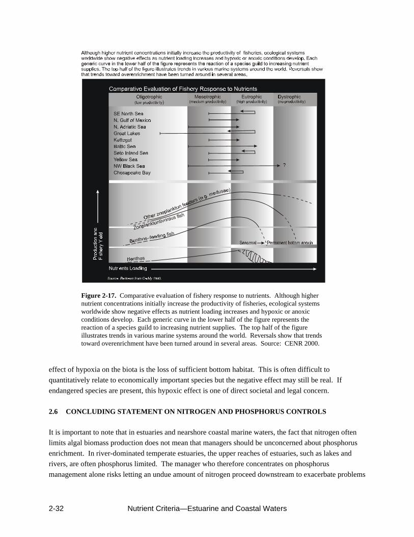
Nutrient Criteria—Estuarine and Coastal Waters2-32
Figure 2-17. Comparative evaluation of fishery response to nutrients. Although highernutrient concentrations initially increase the productivity of fisheries, ecological systemsworldwide show negative effects as nutrient loading increases and hypoxic or anoxicconditions develop. Each generic curve in the lower half of the figure represents thereaction of a species guild to increasing nutrient supplies. The top half of the figureillustrates trends in various marine systems around the world. Reversals show that trendstoward overenrichment have been turned around in several areas. Source: CENR 2000.
effect of hypoxia on the biota is the loss of sufficient bottom habitat. This is often difficult toquantitatively relate to economically important species but the negative effect may still be real. If
endangered species are present, this hypoxic effect is one of direct societal and legal concern.
2.6 CONCLUDING STATEMENT ON NITROGEN AND PHOSPHORUS CONTROLS
It is important to note that in estuaries and nearshore coastal marine waters, the fact that nitrogen oftenlimits algal biomass production does not mean that managers should be unconcerned about phosphorus
enrichment. In river-dominated temperate estuaries, the upper reaches of estuaries, such as lakes andrivers, are often phosphorus limited. The manager who therefore concentrates on phosphorus
management alone risks letting an undue amount of nitrogen proceed downstream to exacerbate problems

Nutrient Criteria—Estuarine and Coastal Waters 2-33
where an abundance of P allows the excess N to drive trophic conditions to unacceptable levels ofnutrient enrichment.
Similarly, any reductions achieved in P loadings and concentrations at the coastal margin will limit
potential eutrophy/hypertrophy even in the face of abundant nitrogen. Consequently, the prudentmanagement strategy is to limit both phosphorus and nitrogen. Emphasis on one or the other as an
element of symptomatic management in fresh or saline waters may be appropriate in some cases, but themanager must always be concerned about the downstream consequences and the net enrichment effects
to the larger system.
In summary, attempting to understand the nutrient overenrichment problem in estuaries and coastalecosystems primarily from a bottom-up perspective provides a limited perspective. This manual has
included references to the historical past that reported on potential positive effects of top-down controlson nutrient overenrichment. It is likely that the most scientifically robust nutrient criteria will need to
take into account the effects of past overfishing and its consequences for marine eutrophication (Jacksonet al. 2001). Thus, higher trophic levels are more than just a thermodynamic response to nutrient
enrichment because they help modulate many of the negative consequences of overenrichment.Ecological feedback mechanisms that involve higher trophic levels can be a positive tool in nutrient
management.

Nutrient Criteria—Estuarine and Coastal Waters 3-1
Major Factors Influencing Estuarine Susceptibility to Nutrient OverenrichmentExamples of Coastal ClassificationCoastal Waters Seaward of Estuaries
CHAPTER 3
Classification of Estuarine andCoastal Waters
3.1 INTRODUCTION
Purpose and BackgroundClassification is an important step in addressing the problem of degradation, especially because ofnutrient overenrichment. There are too many nutrient-degraded estuaries in the United States for theNation to conduct comprehensive ecosystem studies of all those affected by overenrichment. Wherepossible, similar estuaries, tributaries, or coastal reaches should be equated through physicalclassification to reduce the magnitude of the criteria development problem and to enhance predictabilityof management responses. To be useful, classification should reduce variability of ecosystem-relatedmeasures (e.g., water quality factors) within identified classes and maximize interclass variability. Thisis important because managers need to understand how different types of estuaries and coastal waters, aswell as important habitat differences within these systems, respond to nutrient overenrichment in order toplan effective management strategies.
The ecosystem processes that regulate nutrient dynamics, discussed in Chapter 2, should provide theelements for initial development of a useful classification system. Although predicting susceptibility ofestuarine and coastal waters to nutrient overenrichment is in a primitive state, several approaches arereviewed because they have some utility even if they are only marginally adequate for prediction ofnutrient effects. The general approach is also appropriate for coastal systems.
General trends relate N loading with chlorophyll and primary productivity; however, these trends areseldom usefully predictive for individual systems or for all classes of coastal systems (Kelly in press). Progress has been especially slow in predicting many of the secondary, but societally important, effectsof nutrient overenrichment, e.g., bottom water dissolved oxygen (DO) deficiency, harmful algal blooms(HABs) or species-specific HABs, formation of macroalgal mats, fisheries productivity, and speciescomposition. For many cross-system comparisons, N loading and SAV decline have become morepredictive than for other indirect effects (Duarte 1995; Dennison et al. 1993), but even here thepredictions may be confounded by highly variable ecosystem factors. A major impedance to effectiveunderstanding is limited comparative studies designed to test hypotheses regarding estuarinesusceptibility to nutrient enrichment (Turner 2001). Post hoc comparative approaches and assessment ofdisparate studies have been useful but clearly inadequate (Livingston 2001b).
Post hoc statistical approaches have helped explain some of the variability in eutrophication, but have notcaptured the actual mechanisms and their interactions controlling eutrophication across estuaries and
Nutrient Criteria—Estuarine and Coastal Waters3-2
coastal waters (NRC 2000). The ability to explain the mechanisms in a predictive manner is clearly acritical national and global research need, as nutrient overenrichment of coastal ecosystems extends farbeyond the shores of the United States. For site-specific criteria, several approaches are available,including empirical regression and mechanistic simulation models. The large effort typically required tocalibrate and verify mechanistic models is an indicator of the difficulty in understanding the manypotential confounding factors of ecosystem-level prediction. A basic premise of this manual is thatknowledge of the physical setting and the minimally disturbed ecosystem reference condition mustunderpin monitoring and management efforts to protect and restore coastal systems impaired by nutrientoverenrichment.
Only in approximately the past two decades have comparative studies of nutrient dynamics among two ormore relatively large estuaries been published (e.g., Fisher et al. 1988; Malone et al. 1999; Pennock et al.1994). Comparative analysis of the Delaware and Chesapeake Bays has provided insights regardingprocesses that control expression of nutrient enrichment (Chapter 2). For example, both systems aredrowned river mouth coastal plain estuaries and are located adjacent to each other along the coast, buthave very different responses to nutrient loading. Delaware Bay has a somewhat larger nutrient load thanthe Chesapeake, but has few of the nutrient enrichment symptoms well chronicled for the ChesapeakeBay (Flemer et al. 1983, Sharp et al. 1994, Chesapeake Bay Program Periodic Status Reports). Similarinsights have been provided by comparing nutrient processes between Delaware and Mobile Bays(Pennock et al. 1994). Susceptibility appears to be largely explained by differences in the physics offlushing, including bathymetry and related physical habitat differences.
Defining the Resource of ConcernAs a first step in classification, defining the resource of concern is important. Resources of concern areestuaries and coastal waters located in the contiguous States or within authorized Tribal lands. Managersmust decide which waterbodies to include in the population to which criteria will be applicable. A lakeclassification may exempt small ponds that might be excluded because of their size and man-madenature, whereas tidal creeks, although small, still have a functional connection to the larger estuary andmight not be excluded because of size. Many estuaries and coastal waters share multiple politicalboundaries, and for the sake of consistency all involved jurisdictions should jointly decide on the scale ofinclusiveness. For open coastal waters, a State or authorized Tribe’s legal authority may extend for arelatively short distance on the continental shelf, e.g., 3 nautical miles. However, coastal oceanographicprocesses seaward of the statutory limit likely influence nutrient overenrichment processes andexacerbate the difficulty of diagnosing the anthropogenic contribution to nutrient problems.
3.2 MAJOR FACTORS INFLUENCING ESTUARINE SUSCEPTIBILITY TONUTRIENT OVERENRICHMENT
The NRC (2000) publication summarized approximately a dozen factors deemed important tocharacterize the susceptibility of estuaries to nutrient loading. A short list is provided; however, it isexpected that the following list will be modified and refined as more is learned about the subject:

Nutrient Criteria—Estuarine and Coastal Waters 3-3
1. System dilution and water residence time or flushing rate2. Ratio of nutrient load per unit area of estuary3. Vertical mixing and stratification4. Algal biomass (e.g., chlorophyll a, and chlorophyll a corrected for nonchlorophyll a light
attenuation over seagrass/SAV beds and macroalgal biomass as AFDW)5. Wave exposure (especially relevant to seagrass potential habitat)6. Depth distribution (bathymetry and hypsographic profiles)7. Ratio of side embayment (s) volume to open estuary volume or other measures of embayment
influence on flushing.
Several terms listed above are briefly discussed because their significance often is not adequatelyappreciated.
DilutionThe volume of an estuary affects its ability to dilute inflowing nutrients. Thus, the loading rate ofnutrient per unit volume of the estuary is a better indicator of the potential for exceeding the assimilativecapacity of the estuary as a whole than is the absolute loading rate. This ratio may not express thepotential for local effects near the point of entry into the estuary, as nutrients there are diluted by only afraction of the total estuary volume. The potential for such local effects is reduced if mixing into themain body of the estuary is rapid.
Water Residence TimeEstuaries that flush rapidly (i.e., have a short residence time) will export nutrients more rapidly thanthose that flush more slowly, resulting in lower nutrient concentrations in the estuary. Dettmann (inpress) has derived a theoretical relationship between the mean residence time of freshwater in an estuaryand the increase in the average annual concentration of total nitrogen in the estuary as a result of inputsfrom the watershed and atmosphere. In addition, estuaries with residence times shorter than the doublingtime of algal cells will inhibit formation of algal blooms. Residence time or flushing rate is discussed inmore detail in Appendix C.
StratificationHighly stratified systems are more prone to hypoxia than are vertically mixed systems. Stratification notonly limits downward transport of oxygen from atmospheric reaeration, it also retains nutrients in thephotic zone, making them more available to phytoplankton. In stratified systems, it may be moreappropriate to estimate the dilution potential of the estuary using the volume above the pycnocline ratherthan the entire volume of the estuary.
It is expected that the shortened list will be revised and modified as more is learned about factorsimportant in estuarine and coastal waters classification. Some of these factors will apply to estuaries andothers to coastal waters.

Nutrient Criteria—Estuarine and Coastal Waters3-4
3.3 EXAMPLES OF COASTAL CLASSIFICATION
Scientists and resource managers have used various classification schemes for many years to organizeinformation about ecological systems. As discussed earlier, estuaries and coastal water systems arecharacterized by a suite of factors (e.g., river flow, tidal range, basin morphology, circulation, andbiological productivity) that are ultimately controlled largely by geology and climate. A review ofChapter 6 in the NRC (2000) publication provides useful descriptions of the various approaches toestuarine classification, and some pertinent features are highlighted below.
Geomorphic ClassificationGeomorphic classification schemes provide some insight into the circulation structure and are a first-order estimate of water residence time or flushing characteristics. Such classifications may not inthemselves be predictive of susceptibility to nutrient enrichment, but they are a useful place to begin afirst-order assessment of susceptibility. Knowledge of deep channels, however, identifies potential areassubject to hypoxia, and the extent of shallow waters and associated factors (e.g., wind fetch) oftenprovides insights into potential seagrass habitat.
Estuaries can be divided geomorphically into four main groups (Pritchard 1955, 1967; Dyer 1973): (1)coastal plain estuaries, (2) lagoonal or bar-built estuaries, (3) fjords, and (4) tectonically caused estuaries. This classification frequently appears in textbooks, and only some important features relative to nutrientsusceptibility are described.
Coastal Plain Estuaries: Classical and Salt MarshBoth subclasses are characterized by well-developed longitudinal salinity gradients that influencedevelopment of biological communities. Examples of the classical type include the Chesapeake Bay (thelargest estuary of this type), Delaware Bay, and Charleston Harbor, SC. Vertically stratified systemswith relatively long residence times (e.g., Chesapeake Bay) tend to be susceptible to hypoxia formation. Pritchard (1955) further classified drowned river valley estuaries into four types (A-D) depending on theadvection-diffusion equation for salt (Table 3-1). Type C estuaries are less sensitive to algal bloomformation and hypoxia because of mixing features.
The salt marsh estuary lacks a major river source and is characterized by a well-defined tidal drainagenetwork, dendritically intersecting the extensive coastal salt marshes (Day et al. 1989). Exchange withthe ocean occurs through narrow tidal inlets, which are subject to closure and migration following majorstorms (e.g., Outer Banks, NC). Consequently, salt marsh estuarine circulation is dominated byfreshwater inflow, especially groundwater, and tides. The drainage channels, which seldom exceed adepth of 10 m, usually constitute less than 20% of the estuary, with the majority consisting of subaerialand intertidal salt marsh. These systems are a common feature of the Atlantic coast, particularly betweenCape Fear, NC, and Cape Canaveral, FL. Mangrove estuaries occur from around Cape Canaveral southon Florida’s east coast and on Florida’s west coast from around Tarpon Springs south. Nutrientdynamics, primary production, and system respiration that occur within emergent marshes may greatlyaffect water quality in the estuarine channels (Cai et al. 1999).

Nutrient C
riteria—Estuarine and C
oastal Waters
3-5
Table 3-1. General drowned river valley estuarine characteristics
Estuarine typea
Dominant mixing force
Mixingenergy
Width/depthratio
Salinitygradient
Mixingindexb
Turbidity Bottomstability
Biologicalproductivity
Example
A River flow Low Low Longitudinal vertical
1 V. high Poor Low Southwest Pass Mississippi River
B River flow, tide Moderate Moderate Longitudinal vertical
<1/10 Moderate Good V. high Chesapeake Bay
C Tide, wind High High Longitudinal lateral
<1/20 High Fair High Delaware Bay
D Tide, wind V. high V. High Longitudinal ? High Poor Moderate ?
aFollows Pritchard’s advection-diffusion classification scheme.bFollows Schubel’s definition: MI = equation here (vol. freshwater discharge on ½ tidal period) / (vol. tidal prism).Source: Neilson and Cronin, 1981.

Nutrient Criteria—Estuarine and Coastal Waters3-6
LagoonsLagoons are characterized by narrow tidal inlets and are uniformly shallow (i.e., less than 2 m deep)open-water areas. The shallow nature enhances sediment–water nutrient cycling. Flushing is typically of long duration. Most lagoonal estuaries are primarily wind-dominated and have a subaqueous drainagechannel network that is not as well drained as the salt marsh estuary. Lagoons fringe the coast of theGulf of Mexico and include the mid-Atlantic back bays; Pamlico Sound, NC; and Indian River Lagoon,FL. Although these systems are typically shallow, they may have pockets of hypoxic water subject tospatial variability because of freshwater pulsing and wind effects. Some lagoonal systems have relativelystrong vertical stratifications near the freshwater river mouth and may be subject to hypoxia formation(e.g., Perdido Bay, AL/FL; Livingston 2001a).
Fjords and Fjordlike EstuariesClassical fjords typically are several hundred meters deep and have a sill at their mouth that greatlyimpedes flushing. Hypoxia/anoxia is often a natural feature but anthropogenic nutrient loading canseverely exacerbate the problem. Examples of classical fjords on the North American continent can befound in Alaska and Washington State (Puget Sound). Some other estuaries were also formed by glacialscouring of the coast, but in regions with less spectacular continental relief and more extensivecontinental shelves. Examples of these much shallower, fjordlike estuaries can be found along the Mainecoast.
Tectonically Caused EstuariesTectonically caused estuaries were created by faulting, graben formation (i.e., bottom block-faultsdownward), landslide, or volcanic eruption. They are highly variable and may resemble coastal plainestuaries, lagoons, or fjords. San Francisco Bay is the most studied estuary of this type (Cloern 1996).
Man-Made EstuariesEspecially around the Gulf of Mexico, dredged bayous, canals, and salt water impoundments with weirsfunction as estuaries but do not fit well any of the other types presented. As a special case, especially inthe Gulf of Mexico, the passes of some estuaries periodically were closed off by storms and historicallyremained closed until a natural event reopened them (e.g., Perdido Bay, AL/FL; R. Livingston, personalcommunication). In recent years, these systems typically are maintained in an open condition bydredging. Dredged inlets such as at Ocean City, MD, also fit this classification.
Physical/Hydrodynamic Factor–Based ClassificationsClassification Using Stratification, Mixing, and Circulation ParametersEstuarine circulation was a dominant consideration used in an earlier classification of the ChesapeakeBay, a coastal plain system, and major tributaries, and is largely utilized today with some modifications(Flemer et al. 1983). Coastal plain estuaries are sometimes classified by mixing type: highly stratified,partially mixed (moderately stratified), or well mixed (vertically homogeneous). The flow ratio of theseestuaries (the ratio of the volume of freshwater entering the estuary during a tidal cycle to its tidal prism)is a useful index of the mixing type. If this ratio is approximately 1.0 or greater, the estuary is normally
Nutrient Criteria—Estuarine and Coastal Waters 3-7
highly stratified; for values near 0.25 the estuary is normally partially mixed; and for ratios substantiallyless than 0.1, it is normally well mixed (Biggs and Cronin 1981).
Stratification/Circulation ParametersHansen and Rattray (1966) developed a two-parameter classification scheme based on circulation andstratification of estuaries. Circulation is described by the nondimensional parameter Us/Uf, where Us isthe net (time-averaged) longitudinal surface current and Uf is the cross-sectional average longitudinalvelocity. Stratification is represented by the nondimensional parameter S/So, where S is the top-to-bottom difference in salinity and So is the mean salinity. Jay et al. (2000) review alternative two-parameter classification schemes involving parameters such as the ratio of tidal amplitude to mean depth,along-estuary and vertical density differences and vertical tidal excursion of isopycnals, or other factorsthat take into account effects of tidal flats and provide additional discussion to which the reader isreferred for additional insights. They argue that the merit of the approach is its simplicity of parametersemployed and the predictive ability with regard to salt transport needed to maintain salt balance inmodeling.
Classification Using Water Residence TimeWater residence time, the average length of time that a parcel of water remains in an estuary, influences awide range of biological responses to nutrient loading. The residence time of water directly affects theresidence time of nutrients in estuaries, and therefore the nutrient concentration for a given loading rate,the amount of nutrient that is lost to internal processes (e.g., burial in sediments and denitrification), andthe amount exported to downstream receiving waters (Dettmann in press, Nixon et al. 1996). Residencetimes shorter than the doubling time of algae will inhibit bloom formation because algal blooms areexported from the system before growing to significant numbers. Residence time can also influence thedegree of recruitment of species reproducing within the estuary (Jay et al. 2000).
There are a number of definitions of water residence time, including freshwater residence time andestuarine residence time (Hagy et al. 2000; Miller and McPherson 1991), each with its own interpretationand utility. Freshwater residence time is the mean amount of time required for freshwater entering theestuary to exit the seaward boundary, whereas estuarine residence time is the average residence time inthe estuary for all water, regardless of its origins. Because nutrient loading is generally associated withfreshwater inputs, freshwater residence time is generally the most useful measure in considering estuarysensitivity to nutrient loading. Freshwater residence time of a given estuary is influenced by numerousfactors, including freshwater loading rate (Pilson 1985; Asselin and Spaulding 1993; Hagy et al. 2000),tidal range, and wind forcing (Geyer 1997), and therefore varies over a range of time scales. Residence time and volume together may be used to scale nitrogen loading to estuaries to permitcalculation of nitrogen concentrations and perform cross-system comparisons. Dettmann (in press) usesa model that includes mechanistic representations of nitrogen export and loss within estuaries to showthat [Nu ], the contribution to the annual average concentration of total nitrogen in an estuary from uplandsources (watershed, direct discharges, and atmosphere), may be calculated as

Nutrient Criteria—Estuarine and Coastal Waters3-8
where Ll is the annual average loading rate (mass/month) of total nitrogen from all upland sources(watershed and atmosphere), Jfw is the freshwater residence time in months, V is the estuary volume, and" is a parameter (value = 0.3 month-1) related to losses of nitrogen to processes such as denitrification andburial in sediments within the estuary.
Definitions of residence time, the methods used to measure or calculate them, variability of residencetime, and other estimators of residence time are described further in Appendix C.
River Flow, Tides, and WavesDronkers (1988) proposed an estuarine classification that distinguished various types of estuarineecosystems based on water exchange processes (e.g., river flow, tides, and waves) that greatly affectenergy and material fluxes including mixing (Table 3-2). This classification suggests that river flow inpartially mixed estuaries is essentially neutral, but its variation relative to hydrodynamic residence timecan be important in interpreting property-salinity diagrams (Cifuentes et al. 1990) (Figure 3-1). Riverflow in the partially mixed mainstem of the Chesapeake Bay is seasonally important.
Tidal Amplitude—A Dominant Physical FactorTidal amplitude provides a means to broadly classify estuaries relative to their sensitivity to nutrientsupplies. Monbet (1992) analyzed phytoplankton biomass in 40 estuaries and concluded that macrotidalestuaries (mean tidal range 2 m) generally exhibit a tolerance to nitrogen pollution despite high loadingsoriginating from freshwater outflows (Figures 3-2a, b). These systems generally exhibit lowerconcentrations of chlorophyll a than do systems with lower tidal energy, even when they havecomparable concentrations of nitrogen compounds. Estuaries with mean annual tidal ranges 2 m seemmore sensitive to dissolved nitrogen, although some overlap occurs with macrotidal estuaries.
NOAA Scheme for Determining Estuarine SusceptibilityNOAA (Bricker et al. 1999) developed a categorical approach based on surveys and decision rules thatled to a classification of estuarine nutrient export potential (e.g., dilution potential and flushingpotential). From this information a susceptibility matrix was constructed. The low, moderate, and highsusceptibility indices were combined with low, moderate, and high human levels of nutrient input,resulting in a final matrix of overall human influence (see Appendix D for details).
Comparative Systems Empirical Modeling ApproachThe empirical regression method can be used to determine the response of estuarine systems to nutrientloading. This approach requires that the response factor be common to all systems in the analysis andassumes that any graded response among systems is due to a common form of disturbance, e.g., nutrients. The space-for-time paradigm (Pickett 1988) posits that relationships between nutrient inputs and

Nutrient Criteria—Estuarine and Coastal Waters 3-9
Table 3-2. Classification of coastal systems based on relative importance of river flow, tides, andwaves to mixing
Type River flow Tide Waves Description
I River delta
II River delta (plus barriers)
III Tidal river delta
IV 0 Coastal plain estuary
V Tidal lagoon
VI Bay
VII Coastal lagoonPlus and minus designations indicate relative impacts; e.g., means that river discharge is very small relative to tidaland wave energy.Source: Adapted from Dronkers 1988.
ecologically meaningful estuarine responses, using multiple systems, have predictive capability, at leastfor the systems used in the model development. This allows for a wide range in nutrient loading andestuarine types to be included. The comparative-systems empirical approach has been used to determine,for example, relationships between nutrient inputs and fish yields (Lee and Jones 1981, Nixon 1992),benthic biomass, production and abundances (Josefson and Rasmussen 2000), summer ammonia flux(Boynton et al. 1995), chlorophyll a concentration (Boynton et al. 1996, Boynton and Kemp 2000,Monbet 1992), primary productivity (Nixon et al. 1996), and the dominant source of primary productivity(Nixon et al. in press). In many of these cases, important environmental factors such as flushing time anddepth are used to normalize the nutrient loading in a similar way as Vollenweider (Vollenweider 1976)Did for lakes to yield more precise relationships. Appendix E provides additional details.
Other ConsiderationsHabitat TypeThe presence and extent of different habitat/community types may help distinguish one or more estuarieswithin a region. These types may include seagrasses, mangroves, mudflats, deep channels, oyster reefs,dominance of sand versus mud bottoms, extensive emergent marshes (typically coastal plain systems),and the presence of unconsolidated versus rocky shorelines. Some of these categories may besubclassified by salinity ranges (e.g., oligohaline, mesohaline, and polyhaline). Although related more towater quality, blackwater versus turbid versus relatively clear estuaries defines a group representative ofestuaries around the Gulf of Mexico.
Theoretical ConsiderationsCoastal zone managers may wish to consider more theoretical approaches to classification as ecosystemscience develops a more in-depth understanding of ecosystem processes for estuaries under theirpurview. Several different approaches are described in Appendix F.

Nutrient Criteria—Estuarine and Coastal Waters3-10
Figure 3-1. Idealized micronutrient-salinity relations showing concentration and mixingof nutrient-rich river water with nutrient-poor seawater. Source: Peterson et al. 1975. A. Expected concentration-salinity distribution of a substance behaving in a conservativemanner (e.g., chloride) in an estuary. B. Expected concentration-salinity distribution of asubstance for which the estuary is a source (e.g., particulate carbon). C. Expectedconcentration-salinity distribution of a substance for which the estuary is a sink (e.g.,phosphorus). D. Expected concentration-salinity distribution of a substance for whichthe estuary is a pronounced sink, that is, where the concentration of the substance in theestuary is lower than the river and the ocean (e.g., Si). Source: Biggs and Cronin 1981.

Nutrient Criteria—Estuarine and Coastal Waters 3-11
Figure 3-2a. Relationship between the mean annual loadings of dissolved inorganic nitrogen(DIN) and the mean annual concentration of chlorophyll a in microtidal and macrotidal estuaries.
SummaryVarious ways are available to classify estuaries regarding their vulnerability to nutrient enrichment. None appear to provide all the information a resource manager may want for decisionmaking. TheNOAA estuarine export potential (EXP) appears to have the current greatest utility for predictivepurposes for large systems, but even this approach embodies considerable variability (e.g., see Figures 6-5 and 6-6 in NRC 2000). For embayments within a larger estuary, the comparative empirical modelingapproach has been demonstrated to have considerable utility. The more theoretical models eventuallymay provide greater predictive power, especially as to biological sensitivities to nutrient enrichment. They are data intensive and may become more useful at a future time.
3.4 COASTAL WATERS SEAWARD OF ESTUARIES
Several approaches are available to classify coastal waters. The geomorphic focus is a good place tobegin, hydrographic considerations should follow, and finally habitat and community features should beconsidered. Although functional considerations and theoretical indices are not described for coastalwaters, they have as much relevance for these waters as they do for estuaries. Even though much of theconcern for coastal waters will be within 20 nautical miles of shore, and most of that within the 3-milelimit, elements of the following large-scale classification scheme will have value to the manager andinvestigator.

Nutrient Criteria—Estuarine and Coastal Waters3-12
Figure 3-2b. Relationship between the mean annual concentrations of dissolved inorganic nitrogen (DIN)and chlorophyll a in microtidal and macrotidal estuaries. Source: Monbet 1992.
Geomorphic ClassificationThe flow of energy and nutrients through coastal food webs differs greatly among continental shelves,and is driven largely by differences in the form and amount of primary production (e.g., seagrasses areimportant in the Big Bend area of Florida and kelp forests are important habitats along much of the U.S.Pacific Coast and sections of coastal Maine). These differences in turn ultimately are determined bydifferences in local and ocean-scale patterns of climate (e.g., light and temperature effects), watercirculation, chemistry, and shelf geomorphology (Alongi 1998). The spring bloom, especially along theU.S. Atlantic Coast, generally progresses from low to higher latitudes but with sharper seasonal peakstoward higher latitudes. Variability in the progression should be considered in any classification scheme. Because near-coastal shelf oceanographic processes usually are not limited by the jurisdiction of a singleState, it is important that a similar classification approach be shared among coastal States, where thatoceanography determines the sensitivity of the ecosystem to nutrient enrichment. The geographic extentof the shelf in which a State has jurisdiction is a useful place to begin classification. Here one shouldconsider whether the shelf is wide or narrow (e.g., mid-Atlantic versus Pacific Coast). The Texas coastalshelf is very wide, with a gentle slope compared with much of the northern Gulf of Mexico. Thesteepness of the slope is another useful factor, as it may influence bottom sediment stability and

Nutrient Criteria—Estuarine and Coastal Waters 3-13
upwelling. The degree of bottom roughness or sculpture may influence vertical mixing, which may inturn influence water column stability and depth of the euphotic zone versus mixing depth.
Nongeomorphic ClassificationWalsh characterized the world’s continental shelves on the basis of their location, major rivers, and ratesof primary production, and included some U.S. coastal waters for comparison. The shelf proper is whereoceanic and estuarine boundaries often intermingle. At the shelf edge, cold, nutrient-rich water andassociated materials intrude onto the shelf. There, exchanges often are rapid, promoting conditionsfavorable for higher fertility than in the open ocean. Higher primary productivity is the main reason whyapproximately 90% of the world’s fish catch is harvested on the continental shelves versus the open sea(Alongi 1998).
Water Quality Trend Detection on the ShelfPhysical mixing and advective processes may add considerable variability to water column measures. Therefore, it is important to consider detection of trends in nutrient concentrations and measures such aschlorophyll a based on comparisons at a reference salinity (e.g., 30 psu). Otherwise, classificationschemes may incur extraneous variability. A common approach is to use “mixing diagrams” to comparemeasured changes in an ambient constituent among sampling periods. At mid- and higher latitudes,winter measures of DIN and DIP may provide insight into long-term trends of changes in nutrientconcentrations available to drive the spring bloom. At low latitudes winter values will likely have lessapplicability, as primary production has a smaller seasonal signal.
Presence of Large RiversAlthough large rivers are included in Walsh’s characterization of shelf systems, it seems useful todistinguish shelf areas based primarily on large rivers, such as the Mississippi River in the Gulf ofMexico and the Columbia River off the Washington-Oregon coast. Large rivers on the shelf dominatelocal ecological relationships.
Hydrographic FeaturesVertical salinity differences tend to decrease toward the open ocean boundary. The principal reason issummertime thermal stratification. The thermocline tends to be deeper toward the open sea margin,except where buoyancy effects are associated with large rivers that flow onto the shelf. Coastal waterscontain a variety of biotic communities, including a diverse assemblage of macroepifauna and -infauna,kelp forests, coral reefs, bottom and pelagic fishes, marine mammals, and seabirds. The relationship ofthese communities to physical-ordering factors can assist in classification.
Temperate and subtropical coastal waters also experience a seasonal sea-level fluctuation, wherebysummer levels rise approximately 0.2 m by upper-ocean heat expansion, producing what is known asthermosteric effects (Pattulo et al. 1955, Bell and Goring 1998). This nontidal process operates inconjunction with other factors affecting apparent mean sea level (e.g., near and far-field wind effects andbarometric pressure). Depending on local conditions, water levels overlying the continental shelf and inestuaries can rise from 0.1 to 0.2 m. Such a rise may seem nominal but can have a significant impact in

Nutrient Criteria—Estuarine and Coastal Waters3-14
wetlands and other low-lying areas that potentially exchange nutrients and suspended sediments with thecoastal ocean.
Coastal ocean waters range from quite cold (e.g., Gulf of Maine) to quite warm (e.g., Gulf of Mexico). Where large rivers enter coastal waters, such as the Mississippi River Plume and Chesapeake Bay Plume,visual discoloration can be observed because suspended material from land runoff and relatively highplankton concentrations contrast with the predominantly blue color of the open ocean. The ColumbiaRiver and the Mississippi River form an “estuary” mostly at sea, as very little of the diluted seawater isbounded by land.
Physical gradients are dynamic and change at multiple scales. Seasonal or wet and dry periodsfrequently differ depending on the various shelf gradients associated with estuarine, riverine, andocean/shelf break processes. Regional geomorphology and physical mixing processes play a pivotal rolein energy flow and material cycles. For example, the Loop Current in the eastern Gulf of Mexico mayshow seasonal reversals and vary seasonally in its penetration onto the shelf. Along-shore drift inside thenorth-flowing Gulf Stream off the Mid-Atlantic Bight tends to transport materials southward toward theNorth Carolina coast. Further south, the Gulf Stream forms a seaward boundary that tends tosignificantly isolate in-shore waters from those beyond the shelf break. Local current maps are availablefrom the National Ocean Service of NOAA (www.noaa.gov; then click on nos).
Many different types of boundaries or fronts occur in coastal seas, but no formal classification exists. Alongi (1998) lists five categories:• Shelf-sea (tidal) fronts• Estuarine fronts or plumes• Shelf-break fronts• Upwelling fronts• Island wakes and fronts caused by other land featuresFronts provide increased physical stability at local scales, which may positively influence primaryproduction and energy flow to higher trophic levels (see Chapter 2).
Habitat/Community DifferencesPresence of Mangrove/Seagrass and Coral CommunitiesAlong the southeastern Florida Atlantic coast exists a combination of mangrove, seagrass, and coral reefecosystems. In some localities, each community type may dominate the others, but often they co-occur. Seagrass communities may dominate certain shelf areas along the west coast of Florida (e.g., Big Bendregion). The Flower Gardens, a disjunct coral community, exist off the southern coast of Texas. Alongi(1998) devotes chapters to coral reefs and mangrove ecosystems including factors regulating primaryproductivity (e.g., N and P). The role of N and P enrichment versus grazing in coral reef ecosystems isstill strongly debated in the scientific literature (e.g., Miller et al. 1999). A paper by Chen and Twilley(1999) discusses soil nutrient relationships and productivity in a Florida Everglades mangrove ecosystemalong an estuarine gradient (see the references cited above for the most recent perspective). These

Nutrient Criteria—Estuarine and Coastal Waters 3-15
distinctive ecosystems provide a basis for local coastal waters classification. Mangrove communitiesalso occur along the lower Texas coast, and seagrasses are a dominant community in Laguna Madre, TX.
Presence of SeaweedSeaweeds are common algal communities in rocky intertidal zones (e.g., Fucus spp.), attachingthemselves by means of a holdfast. Seaweeds belong to three marine algal classes: Chlorophyceae(green algae), Rhodophyceae (red algae), and Phaeophyceae (brown algae). The kelps (Laminariales),members of the brown algae, live subtidally but in relatively shallow waters and can form large forestsalong the cooler north Atlantic and Pacific coasts. These communities also may occur in the highersalinity reaches of estuaries. Alongi (1998) provides a discussion of primary production, factors limitinggrowth, nutrient cycling, and grazing in these communities.

Nutrient Criteria—Estuarine and Coastal Waters 4-1
Causal and Response VariablesField and Laboratory MethodsNutrient Enrichment and Ammonia Toxicity
CHAPTER 4
Variables and MeasurementMethods To Assess and Monitor Estuarine/Marine Eutrophic Conditions
4.1 INTRODUCTION
This chapter provides an overview of several measurable trophic state variables that can be used toestablish nutrient criteria for estuaries and nearshore coastal waters. Trophic state variables are those
variables that can be used to evaluate or predict the trophic status or degree of nutrient enrichment ofestuaries and nearshore coastal waters, especially when compared with reference conditions. The primary
variables include two causal variables (TN and TP) and two response variables including a measure ofalgal biomass (e.g., chlorophyll a for phytoplankton or macroalgal biomass (AFDW) and water clarity,
e.g., Secchi depth or electronic photometer), and the addition of dissolved oxygen, as appropriate. Thesevariables are relevant at the national scale to practically all estuaries and are potentially relevant to
nearshore coastal waters.
Several variables are important indicators of nutrient overenrichment for a large number of estuaries, butin many cases the data and supporting science are inadequate for most systems (e.g., algal species
composition). Important secondary variables include seagrass and estuarine submerged aquaticvegetation (SAV) distribution and abundance, macroinfaunal community structure, phytoplankton
species composition, and organic carbon concentrations, respectively. Seagrasses and SAV typicallyprovide important shallow water habitat information, and hypoxia/anoxia are measures of loss of bottom
habitat often associated with deeper waters. Organic carbon (total, particulate, and dissolved) is alsoincluded as a secondary variable because this variable is consistent with Nixon’s (1995) definition of
eutrophication. Changes in benthic macroinfaunal community structure often correlate with organiccarbon enrichment and degree of hypoxia and anoxia (Diaz and Rosenberg 1995). The importance of
algal species composition has implications for food webs (Roelke 2000). These variables are discussedin Chapter 2.
As indicated in Chapter 2, the concentration of the primary nutrient variables may not correlate well with
one or more response variables in estuaries, especially hypoxia or anoxia and measures of phytoplanktonbiomass. In this case, predictive relationships should be attempted with nutrient loads using first
empirical regression models or other statistical approaches if necessary to account for ecosystem-basednonlinearities. Application of mechanistic computer models is another approach (see Chapter 9).
Interpretation of nutrient enrichment indicators, especially for estuaries, is complicated by the interaction
with measures of mixing and flushing as discussed in Chapters 2 and 3. Salinity gradients are associatedwith flushing but also play an important role in the type of biological communities exposed to nutrient

Nutrient Criteria—Estuarine and Coastal Waters4-2
enrichment. These physical considerations must always play a part in nutrient enrichment predictionsincluding establishment of reference conditions as discussed in Chapters 2 and 6.
4.2 CAUSAL AND RESPONSE INDICATOR VARIABLES
Nutrients as Causal VariablesNitrogenNitrogen is one of the most important limiting nutrients of autotrophic assemblages (e.g., phytoplanktonand periphyton) incorporated into estuarine and nearshore coastal marine bioassessments. In those
estuaries where N has been demonstrated to limit algal biomass production, it typically does so at highersalinities along the salinity gradient (Chapter 2). Most research has focused on the role of inorganic-N as
a stimulant to algal biomass production (Stepanauskas et al. 1999). However, about 70% of the dissolvedN transported by rivers worldwide (1012g yr-1 ) is dissolved organic N (DON) (Meybeck 1982). In
contrast to P, control of N sources is more difficult because diffuse gaseous sources of N (N2) can beassimilated directly from the atmosphere by N fixation, a process conducted by a variety of bacteria and
cyanobacteria (blue-green algae). Also, dissolved inorganic N forms, especially nitrite and nitrate, arehighly soluble and do not precipitate easily or sediment out when freshwater enters the brackish zone of
estuaries as inorganic P is likely to do.
Total N measured as a water quality indicator consists of organic and inorganic forms. Although somedissolved organic N may be used for algal growth, especially if remineralized by bacterioplankton
(Carlson and Graneli 1993; Seitzinger and Sanders 1999), it and particulate organic forms participate inalgal biomass production through recycling processes (Chapter 2). In systems with hypoxic or anoxic
conditions, the rate of decomposition is reduced. Although still an open question, apparently relativelylittle of the DON is directly utilized by phytoplankton, except for urea and free amino acids (Antia et al.
1991; Paerl et al. 1999). Dissolved organic N in rainwater (synthetic addition of urea and otherconstituents in bioassays) was shown experimentally to stimulate bacterioplankton and phytoplankton
growth; however, the DON resulted in the dominance of diatoms and dinoflagellates whereasammonium-N stimulated production more of small monads (Seitzinger and Sanders 1999). Further work
is required to test whether this response is widely applicable. Thus, the source of DON can influence thedegree of DON utilization by the microbial community. Inorganic N consists of ammonia, nitrite, and
nitrate N. Ammonia N is a primary product of microbial degradation of organic N, and, if not useddirectly by autotrophic algae and vascular macrophytes and microbial heterotrophs for growth, it may be
oxidized through nitrification to nitrite and nitrate. Varying proportions of organic N may be relativelyrefractive and contribute very little to N overenrichment problems. However, the readily recyclable
component may contribute to N enrichment problems locally and further seaward. Some experimental ormodel analysis (e.g., box model) of the utilization of DON and in some cases particulate organic N for
each coastal system is usually warranted.
In estuaries, N concentrations, especially the inorganic forms, typically vary widely seasonally,interannually, and along salinity gradients. In temperate river-dominated estuaries, nitrate concentrations
may reach very high concentrations (e.g., >100 µM) in tidal fresh to brackish reaches (see Appendix G;

Nutrient Criteria—Estuarine and Coastal Waters 4-3
Neilson and Cronin 1981) due to wash-off associated with various land use activities including point andnonpoint sources (e.g., agricultural cropland). By late spring to early summer, the nitrate concentration
may be below analytical detection limits. Nitrite concentrations seldom reach high levels in surfacewaters due to plant utilization and conversion to nitrate through nitrification. The principal bacteria
genera that mediate nitrification include Nitrosomonas, but species of Nitrosococcus, Nitrobacter, andNitrospina are also important (Sharma and Ahlert 1977, Watson et al. 1981). If dissolved oxygen is
limiting nitrification, then nitrite may accumulate (Helder and de Vries 1983). Ammonia concentrationsin open estuarine and nearshore coastal waters located away from point sources typically vary from
below detection limits to approximately 1.0 to 5 µM, depending on growing season and rates of organicN decomposition. Much higher values may occur for relatively short periods. The ionized form of
ammonia/ammonium is the most abundant reduced form and represents approximately 97% of the total(Sillen and Martell 1964). The equilibration between the ionized and un-ionized fractions is controlled
by temperature, salinity, and pH, resulting in a range of un-ionized ammonia of 1% to 5% of the total attypical salinities, pH, and temperature (Emerson et al. 1975). Ammonia may be toxic to marine larvae,
not just a stimulus to algal growth. Unionized ammonia concentrations in the range of 1.0:Mapproximate those that are known to be toxic to marine larvae, especially molluscs (U.S. EPA 1989).
Denitrification may remove from a few to approximately 50% of the TN load entering temperate
estuaries annually (Seitzinger 1988, Cornwell et al. 1999) depending largely on residence time of the
water, sediment biogeochemical conditions (macroinfauna present to maintain irrigation, oxic conditionsin the overlying bottom water), and water column depth. This process helps to modulate extreme DIN
concentrations (Chapter 2). Typical values for dissolved inorganic N (DIN) and a few TN concentrationsin estuaries and coastal nearshore waters are presented in Appendix G as a basis to help establish
expectations for various coastal systems. It should be noted that N concentrations vary widely in spaceand time and the values in Appendix G are only intended to be rough guides. Specifics of analytical
techniques to measure the various forms of N are included at the end of this chapter (Field Sampling andLaboratory Analytical Methods).
In open coastal waters of the North Atlantic Ocean at temperate latitudes, there is a typical seasonal
progression in DIN and DIP concentrations associated with phytoplankton blooms. The spring bloomreduces these inorganic forms while phytoplankton biomass accumulates. This progression begins at
lower latitudes and moves to higher latitudes. The spring bloom typically crashes in late spring, andsummer biomass levels often are nutrient limited. Often a small bloom occurs in the fall following the
fall thermocline breakdown that allows mixing and replenishment of nutrients from deeper waters intothe upper surface layers, where a short burst of production occurs before light becomes limiting.
Accumulation of deepwater nutrients during the winter has been used to assess the potential for spring-summer overenrichment in coastal seas based on trends in “salinity-nutrient mixing diagrams” (European
Union Northern Marine Eutrophication Criteria Program, Ulrich Claussen, Germany, personalcommunication). Seasonal nutrient patterns in estuaries are quite variable. In some estuarine systems, a
winter buildup of N and P has been observed (e.g., Patuxent River Estuary), especially when freshwaterflows remained low and point sources dominated the nutrient supply (e.g., Flemer et al. 1970). Mixing
diagrams also help interpret nutrient behavior in estuaries; however, some precautions are important torecognize (e.g., see Sharp et al. 1986).

Nutrient Criteria—Estuarine and Coastal Waters4-4
At the interface between fresh and marine waters, a process occurs that results in an apparent increase inthe ionized ammonia concentration. This process is apparently driven by the increased electrolyte
solution of the salts, which has a significant impact on the production and nitrification process, thusyielding higher ionized ammonia levels (Rysgaard et al. 1999). Ionized ammonia adsorption to particles
was decreased, especially in the 0 to 10% salinity range, as were the nitrification and denitrificationprocesses. Further evaluation showed that the reduction in nitrification and denitrification processes was
due not only to the displacement of bacteria and ionized ammonia from particles, but also to decreasedbacterial activity. The projections from these studies were that ionized ammonia would be produced at a
rate of 1 µM/g of sediment in the water. The changes in N dynamics that affect adsorption of suspendedsolids may need to be included when considering acceptable levels in fresh water sources to estuaries.
PhosphorusPhosphorus is an important plant nutrient that may limit algal biomass production in tidal fresh to
brackish zones of estuaries and some subtemperate to tropical marine coastal systems (Chapter 2). Thereare no common stable gaseous forms of phosphorus, so the phosphorus cycle is endogenic, without an
atmospheric component (Manahan 1997). The main natural reservoirs of phosphorus are poorly solubleminerals (e.g., hydroxyapatite) in the geosphere. Erosion of these materials from terrestrial sources and
their transport to the sea are important sources of new phosphorus in seawater. The phosphorus enteringthe sea is mostly orthophosphate, PO4
-3 (Kennish 1989). In previous decades, prior to widespread
phosphate bans in detergents, estuaries received a considerable portion of P from detergents. The banresulted for many estuarine systems in an elevated DIN:DIP ratio. In estuaries and nearshore coastal
waters, phosphorus is present in dissolved inorganic form as well as dissolved and particulate organicform. Some fraction of P may be strongly embedded in a mineral matrix, and this renders that fraction
relatively inert to biological utilization. For this reason, often measures of TP may represent somecomponent that is not biologically available and managers should consider this in developing P criteria.
Plants directly take up the phosphates as essential nutrients during photosynthesis. Some algae have thecapability to break down dissolved organic P (DOP) with alkaline phosphatase (algal and free
phosphatases) and utilize the phosphate as inorganic phosphate (Huang and Hong 1999). Alkalinephosphatase apparently is located on phytoplankton cell membranes, which makes it difficult to
determine whether the uptake is direct for DOP or the DOP undergoes enzymatic hydrolysis on the cellmembrane. Malone et al. (1996) suggested by inference that Chesapeake Bay phytoplankton may utilize
organic sources of P, in part, because the DIN:DIP thresholds approach 160, which is considerablygreater than the N:P ratio reported by Redfield et al. (1963). Orthophosphates are typically preferred by
autotrophic phytoplankton, although some assimilation of organic phosphorus may occur, especiallyduring periods of P deficiencies (Boney 1975). When plants die, or are eaten, the organic phosphorus is
rapidly converted to orthophosphates through the action of phosphorylases within fecal material,phosphatases in the plant cells, and finally by bacteria (Riley and Chester 1971).
To summarize, phosphorus occurs in natural waters and in wastewaters almost solely as phosphates.
These are classified as orthophosphates, condensed phosphates, and organically bound phosphates(common analytes are total phosphorus [TP] and dissolved or particulate organic phosphorus [DOP,
POP]). These compounds may be soluble, in particulates or detritus, or incorporated as organic P in
Nutrient Criteria—Estuarine and Coastal Waters 4-5
organisms. Phosphorus is essential to the growth of organisms and can limit phytoplankton biomassproduction, which is most commonly observed in freshwater systems (Hecky and Kilham 1988) and
some estuaries and coastal marine systems (Chapter 2). In instances where phosphate is limiting, thedischarge of raw or untreated wastewater, agricultural drainage, or certain industrial wastes may
stimulate the growth of algae. Appendix G provides examples of P concentrations in several forms.
SilicaSilica, as an important algal nutrient, has received much less attention in estuarine nutrientoverenrichment studies than N and P based on the limited volume of literature citations (e.g., see Malone
et al. 1996) and recent reviews of estuarine eutrophication (Chapter 1). Silica limitation of diatomproduction, a major algal group that requires Si (and silicoflagellates), often is a measure of N or P
overenrichment (D’Elia et al. 1983; Conley and Malone 1992). Dissolved Si is a product of weatheringand erosion of rocks on land with subsequent transport to the sea (Conley and Malone 1992). Because Si
has essentially no human sources, except possibly from erodible soils under human influence, it is not astrong candidate for regulation. In some parts of the ocean, organisms (such as diatoms and radiolarians)
abound that have produced skeletons of a noncrystalline form of hydrated silica-opal. As these skeletonssettle to the sea floor they slowly dissolve, releasing silica. Officer and Ryther (1980) predicted that
increases in N and P to estuaries and coastal waters from human activities, coupled with the reduction insilicates to the sea from construction of artificial lakes, would alter the N:Si and P:Si ratios. These
alterations were postulated to alter phytoplankton populations to reduce the relative abundance ofdiatoms and enhance the relative abundance of flagellates. Egge and Aksnes (1992) showed that diatoms
always numerically dominated the phytoplankton community when concentrations of silica were inexcess of 2.2 µM. Dominance by diatoms ceased or became more variable when concentrations of Si
were less than this value.
Ryther and Officer (1981) reinterpreted the relationship of N pollution in Long Island Inlets during the1950s. Nitrogen may have limited the nuisance Nannochloris, blooms but they hypothesized that the
bloom persisted because diatoms had been eliminated by Si depletion. Also, the degree of Si limitationof spring diatom blooms in Chesapeake Bay that fuel summer anoxia has direct ecological implications
(Conley and Malone 1992, Malone et al. 1996). Freshwater sources of Si dominate estuarine supplies(Fisher et al. 1988). Typically, Si limitation can be potentially deduced from ambient ratios relative to
the nutrient-sufficient N:Si:P biomass ratios of 16:16:1 (Redfield et al. 1963; Conley et al. 1993). InChesapeake Bay, the dissolved Si:DIP ratio often approximates 100-300 (Malone et al. 1996), suggesting
strong Si limitation. Significant increases in Mississippi River N and P concentrations and loading anddecreases in silicate have occurred during the 20th century (Rabalais et al. 1996). The increased P
loading and associated increased diatom production and eventual burial in river sediments, as predictedby Officer and Ryther (1980), has resulted in a reduced Si supply to the coastal environment. The
consequence is that diatom production, generallly a preferred phytoplankton group to support highertrophic levels, is now more Si limited than in previous decades. The N:P:Si ratios on coastal Louisiana
and Texas now suggest the possibility of a joint nutrient limitation of phytoplankton production.
Nutrient Criteria—Estuarine and Coastal Waters4-6
Silica concentrations for the Coastal Texas/Louisiana coast averaged approximately 5.3 µM in the late1980s but averaged about 9.0 µM during the early 1960s. Silicate concentrations in the Chesapeake and
Delaware Bays and the Hudson River Estuary ranged from about 90 to near detection levels, 30 to neardetection limits, and 30 to 3 µM, respectively (Fisher et al. 1988). Eyre and Balls (1999) reported that Si
was less likely to limit diatom production in tropical estuaries than in temperate ones becauseconcentrations tend to be much higher in tropical estuaries.
The role of silica may be more important to diatom species composition and food quality as future
research may document. More attention in the future should be given to the measurement and assessmentof the role of Si in estuarine and nearshore coastal primary productivity and food web dynamics and as a
basis for controlling co-limiting N and/or P.
Response VariablesChlorophyll a and Macroalgal Biomass
Chlorophyll a is the molecule mediating photosynthesis in most all green plants (except prochlorophytes,
which contain divinyl chlorophyll), including phytoplankton; it is relatively easy to measure eitherspectrophotometrically or by fluorescence and is commonly used to indicate phytoplankton biomass.
However, the amount of chlorophyll per cell can vary widely. Conversion factors from weight ofchlorophyll to weight of carbon (a desired biomass unit) can vary by a factor of 10. Adaptation to light
levels is the primary reason for observed variability; photoadaptation can cause the chlorophyll per cellto vary widely. The technology for measuring chlorophyll has greatly improved over the decades. The
Welschmeyer (1994) fluorometric analysis reduces the interference due to chlorophyll b andphaeopigments. The HPLC procedure is capable of detecting and quantifying various pigments
characteristic of different algal groups (e.g., diatoms, cyanophyta, chlorophyta, and dinoflagellates)(Jeffery et al. 1997).
Rapid proliferation or blooming of phytoplankton, as reflected in chlorophyll a measurements, occurs
throughout the ocean but is most often associated with temperate coastal and estuarine waters and athigher latitudes. In winter months, growth of phytoplankton populations is generally minimal because of
insufficient light and also because a turbulent and unstable upper water column carries the phytoplanktoncells below the euphotic zone (where light is not sufficient) before they can divide.
Chlorophyll a concentrations vary widely as a function of nutrient supply, water column stability,
euphotic zone depth (light availability), sinking, grazing, disease organisms (e.g., viruses), andflushing/mixing (Chapter 2). Values in excess of 12 to 15 µg/L are likely to cause severe shading of
seagrasses (Kelley in press). Concentrations in estuaries during summer optimum growing conditionsmay exceed 50 to 80 µg/L when nutrient loading is high (Monbet 1992). Summer values in the range of
20 to 40 µg/L are frequently observed in enriched estuaries. In contrast, concentrations in overenrichedtemperate U.S. estuaries during the winter may decrease to 1 to 5 µg/L Nearshore coastal areas removed
from high nutrient loads may experience chlorophyll concentrations in the range of approximately 1 to 3 µg/L (Appendix G). Very high values may occur during the summer under conditions of high levels of

Nutrient Criteria—Estuarine and Coastal Waters 4-7
nutrient enrichment (e.g., the Mississippi River Plume on the Texas/Louisiana Shelf [Rabalais et al.1996]).
Macroalgal biomass, especially benthic unattached forms (i.e., Ulva spp.), often becomes abundant in
relatively shallow estuaries that experience nutrient overenrichment. In estuaries that receive most oftheir nutrient load from groundwater (e.g., Waquoit Bay, Cape Cod, MA; see Chapter 2) benthic
macroalgae may shade out seagrasses. Continued enrichment typically leads to reduction of macroalgaeas phytoplankton predominate in the water column. Macroalgae are difficult to adequately sample for
chlorophyll a, and thick mats often contain sheets of algal material that has begun to degrade. The mostcommon method to sample benthic macroalgae is to collect samples and express the biomass on a dry
weight basis.
Measures of Water ClarityLight Attenuation CoefficientThe Secchi disc has been a mainstay as a tool in estimating water clarity; however, this simple and
inexpensive tool does not provide all of the information required to distinguish the light attenuationeffects of living phytoplankton pigments (i.e., traditionally estimated by chlorophyll a) from other factors
(e.g., inorganic suspended sediments, organic nonchlorophyll-based detritus, and humic-like materials)that reduce water clarity. EPA’s Chesapeake Bay Program (Chapter 2) has developed an analytical
approach that partitions the effect of chlorophyll a from total suspended solids that contribute toreduction in water clarity. This approach has been used successfully in estimating the combined factor
contribution to light attenuation over submerged aquatic vegetation beds (Dennison et al. 1993). Inturbid coastal waters, the analyst should be aware of lower values for the constant 1.7 to estimate the
light attenuation coefficient (see Giesen et al. 1990 and references in Chapter 2). More precise estimatesof the light attenuation coefficient can be made with electronic submersible light meters including PAR
meters (photosynthetic active radiation) and submersible spectral radiometers. These meters are now inwidespread use, and their use should be encouraged because they give a direct measure of light
attenuation, especially in shallow water where depth may limit use of the Secchi disc.
Attenuation of light in the sea in nonalgal bloom areas is determined principally by the amount ofsuspended matter present, but in estuaries and nearshore coastal waters, color from humic-like materials
may significantly compete with particulate material in light attenuation. In moderately turbid coastalwaters, 1% of the surface visible light energy may penetrate to a depth of only 10 to 20 m, but in shallow
estuaries depths often are from 10 cm to 3 m or so. There typically is a strong seasonal variability inwater clarity in temperate estuaries between the active growing season and the winter, and in
subtemperate to tropical estuaries water clarity often is a function of the wet season. In the Atlantictemperate open coastal areas with the coming of spring, the depth of the euphotic zone often increases
and the depth of the mixed layer decreases because of the development of the seasonal thermocline. Thisallows a spring bloom to develop. The thermocline tends to confine the algal cells to the euphotic zone,
which becomes rich with nutrients as a result of winter mixing. In estuaries, the pycnocline may alsohave this effect. In partially mixed estuaries where light is adequate at depth, diatoms may grow below
the pycnocline (Malone et al. 1996). If the necessary growth-promoting factors are also present,

Nutrient Criteria—Estuarine and Coastal Waters4-8
conditions are optimal for proliferation of phytoplankton from seed stock, which may be either theplankton cells themselves or their resting stages (Riley and Chester 1971).
Secchi DepthThe Secchi disc is a useful tool to estimate water clarity (Holmes 1970). Secchi disc measurements often
have a longer historical record than electronic measurements, which facilitates assessment of trends inwater clarity. Secchi depth measurements are obtained with a 40 cm plastic or metal Secchi disk that is
either white or is divided into black and white quadrants on a nonstretchable line that is calibrated indecimeters. The disc should be weighted to maintain a level position, especially under strong current
conditions. The disk is lowered into the water until it disappears from view and the depth is recorded. The disk is then slowly raised to the point where it reappears and the depth is recorded again. The mean
of these two measurements is the Secchi depth. Observations are made from the shady side of the vesselto reduce problems of glare; however, when a small boat is used for field work a “viewing tube” allows
readings under full sunlight conditions. Measurement should be made without sunglasses.
Dissolved OxygenDissolved oxygen (DO) is an integrative measure of ecosystem health and habitat function. As a first-
order estimate, the percent saturation of surface and bottom waters is an index of theproduction/respiration ratio. Dissolved oxygen in bottom waters serves as a measure of habitat
availability for benthic animals and pelagic animals that feed on the bottom. EPA has developedsaltwater DO criteria for coastal waters between Cape Cod and Cape Hatteras (see
www.epa.gov/ost/standards/dissolved). Profiles of DO are indicative of oxygen depletion conditionssuch as hypoxia and anoxia. Lack of oxygen in bottom waters causes sediment to release dissolved
nutrients including orthophosphorus, ammonia, and in addition, toxic hydrogen sulfide.
Carbon CompoundsOrganic matter content is typically measured as total organic carbon (TOC) and dissolved organic carbonand is an essential component of the carbon cycle. The rate of organic carbon production and
decomposition and the resulting microbial biomass are at the heart of the eutrophication problem. Evaluation of the carbon-containing compounds in an aquatic ecosystem can indicate its organic
character. The larger the carbon or organic content, the greater the growth of microorganisms that cancontribute to the depletion of oxygen supplies. TOC is a more convenient and direct expression of
organic carbon content than are the biochemical oxygen demand (BOD), assimilable organic carbon(AOC), or chemical oxygen demand (COD) methods. TOC is independent of the oxidation state of the
organic matter and does not measure other organically bound elements, such as N and hydrogen, orinorganics that can contribute to the oxygen demand measured by BOD and COD. In spite of its
versatility, TOC does not provide the same kind of information as BOD, AOC, or COD, and should notbe used to replace these methods.
At the surface of the sea, the concentrations of particulate and dissolved organic carbon range up to 12.5
µM and between 75 and 150 µM, respectively. In coastal environments, concentrations of dissolved andparticulate organic carbon are greater by factors of ~7-fold. Concentrations of dissolved and particulate

Nutrient Criteria—Estuarine and Coastal Waters 4-9
organic carbon in surface waters are equivalent to 150 to 1,800 µg C/L (Millero 1996). Organic carbonrepresents approximately 50% of the dissolved and particulate organic material in seawater (Millero
1996). However, the major form of carbon in seawater is associated with inorganic carbonate systems.
Benthic MacroinfaunaBenthic macroinfauna are an important biological component of estuarine and nearshore coastal marine
ecosystems. These communities contribute to benthic food webs, contribute to nutrient cycling andsystem productivity through benthic-pelagic coupling of nutrient recycling, help stabilize bottom habitats,
and contribute to marine biodiversity. Benthic infaunal communities are quite diverse within an estuaryor coastal region. Diversity is a function of salinity, with higher diversities associated with higher
salinities (Carriker 1967). Sediment irrigation provided by benthic infauna enhances denitrification byincreasing the flux of ammonium into oxic microenvironments where nitrification can occur and the flux
of nitrite and nitrate into the anoxic sediment zone where denitrification becomes possible (Chapter 2).
4.3 FIELD SAMPLING AND LABORATORY ANALYTICAL METHODS
The following sections provide additional information on field sampling and laboratory methods forselected variables. A list of suggested methodologies for analysis of biochemical parameters is provided
in Table 4-1. These methods have been summarized from nationally or regionally recognized referencecompendiums (APHA 1998, ASTM 1976, U.S. EPA 1979, Spotte 1992) and provide acceptable methods
for determining the concentrations of nutrients as well as acceptable methods for measuring the effects ofthose nutrients in estuarine and marine waters.
Field Sampling MethodsNutrients, Hydrography, and SedimentsPhysiochemical profiles should be recorded for each field sampling station. Important parameters to bemeasured include water temperature, pH, dissolved oxygen, salinity, light attenuation, surface radiation,
and total depth. Generally, a multiparameter water quality instrument CTD is used. Sampling depth willvary depending on specific objectives; however, enough vertical depth reading should be taken to
characterize the physical structure of the water column. For example, CDT measurements might be takenat frequent intervals in the vicinity of the pycnocline (e.g., every 0.1 m in highly stratified estuaries).
Overall current dynamics can be mapped with oceanographic tools such as current meters, drift cards,and acoustic Doppler sounders.
Field sampling of discrete water samples for laboratory analysis can be performed using standard
nonmetallic plastic water bottles. Samples are drawn into prelabeled bottles and fixatives are applied asappropriate to the subsequent analysis. Nutrient and organics samples are stored on ice until reaching a
shoreside sample handling location. Nutrient samples are filtered using graduated syringes and thenfrozen. Samples for total TN and TP are filtered or unfiltered as appropriate, and 20 mL of sample is
frozen for analysis. See Chapter 5 for additional sampling protocols.

Nutrient Criteria—Estuarine and Coastal Waters4-10
Table 4-1. Suggested methods for analyses and monitoring of eutrophic conditions of coastal and marineenvironments (* = primary EPA preferred causal and response variables)
Eutrophication indicators Suggested methodsDetection limit
or rangeComments References
Field
*Water clarity Secchi depth 0.1 m — EPA 903-R-96-006
pH CTD probe 0.01 pH — —
Dissolved oxygen CTD probe 0.02 mg DO/L or Winkller Azide Mod. —
Salinity Salinometer 0.1 psu — —
Light attenuation Sensor 0.05%@100%lighte.g., LI-COR-LI-192S A
sensor—
Temperature CTD probe 0.1°C — —
Laboratory analyses
*Total phosphorus SM 4500P-E 0.3 µM Ascorbic acid method APHA 1998
(including orthophosphate,
SM 4500P-E 0.32 µM Auto. persulfate method APHA 1998
POP, and DOP) EPA 365.2 — — EPA 600/4-79-020
CBP IV.D.2 0.03 µM Auto. persulfate method EPA 903-R-96-006
Dissolved orthophosphate
CBP IV.D.3 0.02 µM Ascorbic acid method EPA 903-R-96-006
Particulate phosphorus CBP IV.D.4 0.04 µM Ascorbic acid method EPA 903-R-96-006
*Total N, incl. DON, SM 4500N-C 0.36 µM Persulfate method APHA 1998
DIN, and PONa ASTM D3867 0.7-143 µM Persulfate method ASTM 1976
EPA — Persulfate method EPA 903-R-96-006
EPA-AERP18 — — EPA 600/4-87-026
CBP IV.D.8 1.9 µM Auto. persulfate method EPA 903-R-96-006
Total Kjeldahl N SM 4500org-C with — Semi-micro-Kjeldahl method APHA 1998
SM 4500NH3-H 1.4-1429 µM Auto. phenate method APHA 1998
EPA 351.3/.1(mod.)
— Colorimetric/titration EPA 600/4-79-020
Ammonia/ammonium SM 4500NH3-B/H 1.4-1429 µM Auto. phenate method APHA 1998
EPA 350.1 0.7-1429 µM Colorimetric phenate EPA 600/4-79-020
CBP IV.D.7 0.3 µM Auto. phenate method EPA 903-R-96-006
Nitrate SM 4500NO3-F 35.7-714 µM Auto. cadmium reduction APHA 1998
EPA 353.2 — — EPA 600/4-79-020
Nitrite SM 4500NO3-F 35.7-714 µM Auto. cadmium reduction APHA 1998
EPA 353.2 — — EPA 600/4-79-020
SM 4500NO2-B 0.7-71 35.7-714 µM Colorimetric method APHA 1998
EPA 354.1 — — EPA 600/4-79-020

Table 4-1. Suggested methods for analyses and monitoring of eutrophic conditions of coastal and marineenvironments (* = primary EPA preferred causal and response variables) (continued)
Eutrophication indicators Suggested methodsDetection limit
or rangeComments References
Nutrient Criteria—Estuarine and Coastal Waters 4-11
CBP IV.D.5 0.01 µM Auto. colorimetric method EPA 903-R-96-006
Nitrate + nitrite SM 4500NO3-F 35.7-714 µM Auto. cadmium reduction APHA 1998
EPA 353.2 — — EPA 600/4-79-020
EPA 4.1.4 0.7-143 µM Technicon autoanalyzer EPA 503/2-89/001
CBP IV.D.6 0.01 µM Auto. colorimetric method EPA 903-R-96-006
Particulate N CBP IV.D.8.10 1.36 µM Filtration/combustion EPA 903-R-96-006
Total organic carbon SM 5310TOC-D >0.1 mg C/L Wet oxidation method APHA 1998
SM 5310TOC-C >0.01 mg TOC/L Persulfate method APHA 1998
EPA 415.1 — — EPA 600/4-79-020
Dissolved organic carbon
SM 5310TOC-C >0.01 mg TOC/L Persulfate method APHA,1998
EPA 415.1 — — EPA 600/4-79-020
ASTM D2574-79 — — ASTM 1976
CBP IV.D.10 0.5 mg/L Catalytic combustion EPA 903-R-96-006
Particulate carbon CBP.IV.D.9 0.097 mg/L Filtration/combustion EPA 903-R-96-006
Total silicates SM 4500SiO2-D 0.33-0.83 µM Heteropoly blue method APHA 1998
ASTM D859-68 — — ASTM 1976
CBP-IV-15 0.17-23.3 µM EPA 903-R-96-006
EPA 370.1 — — EPA 600/4-79-020
CBP IV.D.15 0.22 µM Molybdosilicate method EPA 903-R-96-006
Total suspended solids SM 2540-D 2-20,000 mg/L Dried at 103-105°C APHA 1998
CBC IV.D.13 2.0 mg/L Filtration/heat EPA 903-R-96-006
Total volatile solids SM 2540-E — — APHA 1998
Estuarine — — EPA 430/9-86-004
BOD SM 5210-B — 5-day method APHA 1998
EPA 405.1 — — EPA 600/4-79-020
CBP IV.D.11 — 5-day method EPA 903-R-96-006
COD SM 5220-D — — APHA 1998
EPA 410.4 — — EPA 600/4-79-020
Biological measures
Phytoplankton biomass — — — —
Zooplankton biomass
Chlorophyll ab SM 10200-H 0.01 mg/M3 Fluorometric, HPLC, Spectro. APHA 1998

Table 4-1. Suggested methods for analyses and monitoring of eutrophic conditions of coastal and marineenvironments (* = primary EPA preferred causal and response variables) (continued)
Eutrophication indicators Suggested methodsDetection limit
or rangeComments References
Nutrient Criteria—Estuarine and Coastal Waters4-12
EPA AERP12 — — EPA 600/4-87-026
ASTM D3731-79 Spectrophotometer ASTM 1976
CBP IV.D.12 1.0 µg/L Spectrophotometer EPA 903-R-96-006
Phaeophytin SM 10200-H 0.01 mg/M3 Fluorometric, HPLC, Spectro. APHA 1998
EPA AERP12 — — EPA 600/4-87-026
ASTM D3731-79 — Spectrophotometer ASTM 1976
CBP IV.D.12 1.0 µg/L Spectrophotometer EPA 903-R-96-006
Dinoflagellate density — — — —
Diatom density — — — —
Dinoflagellate/diatom — — — —
Perennial plant density — — — —
Ephemeral plant density — — — —
Epiphytic growth — — — —
Phytoplankton blooms — — — —
Fish kills — — — —a DON, dissolved organic N, DIN, dissolved inorganic N; PON, particulate organic N.b Phytoplankton segments: The HPLC procedure is capable of detecting and quantifying various pigments characteristic ofdifferent algal groups (e.g., diatoms, cyanophyta, chlorophyta, and dimoflagellates) (Jefferey et al. 1997).
Nutrient Criteria—Estuarine and Coastal Waters 4-13
Laboratory Analytical MethodsDetailed methods and references are given in Table 4-1. Some general considerations are presented in
the following sections.
Water Column Nutrients Nitrogen CompoundsSeveral methods have been used to determine the concentration of N species in the marine environment.
Methods presented in this document are relatively easy to use, do not require extensive instrumentation,provide detection limits below those expected in marine environments, and are in general use by many
investigators. The most common forms of N in eutrophication evaluation in order of decreasingoxidation state are nitrate, nitrite, ammonia, and organic N. The sum of these is expressed as TN and is
not to be confused with total Kjeldahl N (TKN), which is the sum of organic N and ammonia. Total Ncan be determined through oxidative digestion of all digestible N forms to nitrate, followed by
quantitation of the nitrate. Nitrite is an intermediate oxidation state of N, both in the oxidation ofammonia to nitrate and in the reduction of nitrate. Such oxidation and reduction may occur in
wastewater treatment plants, water distribution systems, or natural waters. Ammonia is produced largelyby deamination of organic N-containing compounds and by hydrolysis of urea. The two major factors
that influence selection of the method to determine ammonia are concentration and presence/absence ofinterferences (e.g., high concentrations of colored organic substances such as humic-like materials or
paper mill effluents).
Total N is measured by the persulfate method, which digests all organic and inorganic – containingcompounds. All N-containing materials (except nitrogen gas) are measured after sample digestion has
occurred. Various organizations have adjusted sample volume or automated the process and produceddifferent ranges of detection. The lowest detectable concentration is ~ 0.7 µM of TN. This is in the
range of the measured available N (0.7 to 5.0 µM TN) for studies performed off the continental shelf inthe North Atlantic from 1956 to 1958 (Kennish 1989). Kjeldahl N minus the ammonia concentration is
the surrogate measurement for all organic N-containing compounds.
Ammonia/ammonium is measured by the indophenol blue (= phenate) or specific ion electrode methodsafter conversion of ammonia and ammonium to ammonia. This is done by raising the pH of the sample
above 11. This method has some essential features (e.g., minimal interference from waters highly stainedwith humic materials and paper mill effluents); however, the level of detection is relatively high (e.g., 2.0
µM NH3-N) but adequate for ammonia-rich waters (Flemer et al. 1998). Ammonia electrodes do notwork directly in seawater. In the spectrophotometric methods, the ammonia is reduced to
monochloramine and then reacted with phenol to form a blue color. In the specific ion electrode method,the ammonium is converted to ammonia using a strong basic solution and partial pressure of ammonia
gas (i.e., free ammonia) in solution, which is related to the dissolved ammonia concentrations by Henry’sLaw.
Nitrates and nitrites are measured in combination using the cadmium reduction procedure of Wood et
al. (1967). This colorimetric method determines the concentration of these two materials after reaction

Nutrient Criteria—Estuarine and Coastal Waters4-14
of nitrites to produce an azo dye, the color of which is proportional to the concentration of the combinednitrates and nitrites. Total nitrate is determined by subtracting the concentration of nitrite from the
combination of the two. The process for measurement of nitrite produces the same azo dye as thecombined measure, but without the Cd reduction. The difference in these two measures is the nitrate
concentration.
PhosphorusThe target detection limit for measurement of P in seawater is ~ 0.3 µM. The procedures for themeasurement of total particulate and dissolved P as well as orthophosphate in seawater provide detection
limits that are less than this value (U.S. EPA 1996). These procedures convert the phosphorus-containing compounds to orthophosphate through the digestion of the sample with alkaline persulfate.
This treatment is then reacted with ammonium molybdate and antimony potassium tartrate in acidicsolution to produce an intense blue complex with ascorbic acid. Interferences with elevated
concentrations of Si can be avoided by maintaining an acid concentration in the reagents and analyzingthe material at elevated temperatures of ~37°C. The resulting phosphomolybdic acid reduction produces
a purple-blue complex that is measured at 885 nm on a spectrophotometer. This method of measuringreactive silicate is recommended in Millero (1996).
Silica The target detection limit for measurement of Si in seawater is ~0.7 µM. Producing pigmented
silicomolybdate complex by procedures contained in U.S. EPA (1996) provides adequate sensitivity afterthe samples are filtered (0.45 µm GF/F filter) to remove interfering particles and turbidity, and after the
interferences of phosphates and arsenates are removed with oxalic acid. The resultant filtrate is treatedwith a solution containing metol-sulfate (p-methyl-amino-phenol sulfate) to produce a blue color that is
evaluated more efficiently than the yellow color recommended for evaluation in U.S. EPA (1996), with aspectrophotometer at 812 nm (Strickland and Parsons 1968). This method of measuring reactive silicate
is also recommended in Millero (1996).
CarbonTotal carbon consists of inorganic and organic forms that are in particulate and dissolved size classes. The distinction between total and organic carbon is based on acidifying samples to remove the inorganic
forms and filtering through 0.45 µm GF/F filters to remove the particulate forms. Total carbon ismeasured by burning the sample to release the particles contained on the glass fiber filter. This converts
the carbon to CO2, which is then transported to a thermal conductivity detector for measurement. Thecarbon left behind in the filtrate is catalytically combusted using a platinum catalyst at ~680°C that is
then transported to a nondispersive infrared detector. The EPA methods (U.S. EPA 1996) will provideadequate detection of both dissolved and particulate carbon in the total and organic phases. The
difference in total carbon and organic carbon represents the inorganic fractions that are primarily CaCO3
shells.

Nutrient Criteria—Estuarine and Coastal Waters 4-15
Sediment AnalysesBulk SedimentCores are collected from field sites to help determine the historical record and sedimentation rate. Short
cores, the upper 30 cm of the substrate, can be obtained with a HAPPS core, designed to collect arelatively undisturbed core of surficial sediment (Kannerworff and Nicolaisen 1973) and used to profile
sedimentary particulate organic carbon and N. Carbon-N analyses follow the method of Hedges andStern (1984); samples for dissolved constituents in pore water are extracted either by whole-core
squeezing or by centrifugation (Devol et al. 1997, Brandes and Devol 1995, Lambourn et al. 1991). Deepcoring devices are used to collect continuous sediment core samples 2 to 3 m into the sediment bed.
These deeper cores are used for analysis of 210Pb, carbon and N, sulfide, and biogenic silica in order todetermine burial rates of 210Pb and 210Ra.
The sedimentation rate is estimated based on the change in activity of naturally occurring 210Pb
radionuclide produced at a constant rate from the decay of 210Ra, using the excess 210Pb inventory methodof Anderson et al. (1987). Excess 210Pb is determined from the difference between total 210Pb activity in
the sediment and the activity of the background 210Pb being produced from 210Ra. To collect samples formeasurement of 210Pb and 210Ra activity at depth with the sediment, cores are sectioned and each section
is then homogenized and placed in a precleaned 16 oz jar, with a small subsample removed and placedinto a glass vial for particulate C and N analysis (Evans-Hamilton, Inc. 1998).
The excess 210Pb inventory method yields accumulation rates (g/(cm2/yr)), which are converted to a
sedimentation rate (cm/yr) using the bulk sediment density g/cm3. For evaluation of seasonal trends, theupper cm is subsampled at 0.25 cm intervals, and in 1 cm intervals below the first cm, following the
assumption that any seasonal storage of N or carbon would manifest almost entirely at the surface of thesediment.
Pore Water Profiles
Pore water profiles of manganese, iron, nitrate, and oxygen demonstrate that oxidation of iron andmagnesium yields less energy than does oxidation of carbon by oxygen or nitrate. Consequently,
concentration peaks of these species are located below the depletion depths of oxygen and nitrate. Inanaerobic environments, after the supplies of oxygen, nitrate, manganese, and iron are exhausted, sulfate
reduction is the dominant mode of organic matter oxidation and nutrient remineralization.
Sulfate reduction rate can be measured with the radiotracer method of Christensen et al. (1987). Asignificant fraction of the oxygen flux may be consumed by the reoxidation of sulfide produced during
sulfate reduction (Canfield 1993).
Sediment traps are used to measure the quantity and composition of the flux of materials settling throughthe water column to the sediment. There are four materials of interest: chlorophyll as an indicator of
planktonic algal remains, pheaopigments as an indicator of degraded plankton that has been consumed byzooplankton, particulate organic carbon (POC), and particulate organic N (PON). Total sedimentation
rate is corrected for resuspension materials in order to derive the net flux to sediment. Samples are

Nutrient Criteria—Estuarine and Coastal Waters4-16
collected by in situ benthic flux chambers, and measurements of oxygen, silicate, nitrate, ammonium,phosphate, and N gas are made (Evans-Hamilton, Inc. 1998).
Determination of Primary ProductivityPrimary productivity refers to the growth rate of the phytoplankton community and is commonlymeasured using trace amounts of radioactive carbon (as bicarbonate) that label the photosynthetic
reaction. Additional variables are measured to support these data: biomass (as estimated by chlorophylla), incoming solar radiation, and nutrient concentrations at depth. Primary productivity, P, is defined as
P = µ × B
where µ is the specific growth rate (growth normalized per cell) and B is the biomass of the
phytoplankton population (amount of cells). These variables are > ‘compound’ = as they in turn dependon other variables. Growth rate depends on light (solar radiation), dissolved nutrients in the water
column, and water temperature. The phytoplankton biomass is determined by the net result of growthand loss (grazing, mixing, sinking) processes and reflects enrichment conditions.
To estimate primary productivity, samples are collected at varying depths corresponding to
predetermined light levels. Fresh samples at each light level are collected for analysis of chlorophyll a,nutrients, and primary productivity in two sets of two clear bottles and one dark bottle; each set is filled
for ambient treatment and nutrient spike treatment. Nutrient spiking consists of adding an initialconcentration of 10 µM N (NH4CL) and 1 µM phosphorus (KH2PO4) to seawater. Nutrients are
monitored from additional samples collected and tested for nitrate, nitrite, ammonium, orthophosphate,and silicate. Samples are inoculated with 14C-labeled sodium bicarbonate and, if appropriate, the nutrient
spike, and placed in a screened bag to simulate the light level from which they were collected. Samplesare incubated at in situ conditions for 24 hours and then transported to the laboratory for filtration using
glass fiber filter paper (Whatman GF/F, nominal pore size 0.7 µm or smaller pore size). The filters areplaced into vials containing EcoLume scintillation cocktail. The specific activity of the filtered
particulates is measured in a scintillation counter. Primary production is calculated as mg C/(m3/day)using the basic equations found in Parsons et al. (1984) (Evans-Hamilton, Inc. 1998).
In productive coastal waters, measurements using the light and dark bottle technique with changes in
dissolved oxygen often can be used in place of the 14C method (Strickland and Parsons 1968). In somecases, free water gas-based (e.g., DO) methods are possible to measure ecosystem metabolism (Odum
1956; Odum et al. 1959; Kemp and Boynton 1980).
Phytoplankton Species CompositionSamples collected from the field are analyzed to identify and enumerate autotrophic phytoplankton, as
well as heterotrophic dinoflagellates and microzooplankton species. From 20 to 50 mL aliquots ofsamples are settled in separable counting chambers for at least 24 hours before examination under
phase-contrast optics with an inverted microscope following the classic Utermöhl technique (Lund et al.1958). A single transect across the center of the chamber is counted at 390× magnification for

Nutrient Criteria—Estuarine and Coastal Waters 4-17
flagellates; 150× magnification is used for other organisms. From 25% to 100% of the chamber bottomis examined, depending on cell concentrations in the sample. Appropriate multipliers are used to convert
all counts to common units of cells/L (Sournia 1978). Organisms are identified to the lowest taxonomiccategory possible. Even quite small changes in the physical and chemical parameters and availability of
micronutrients can have a significant effect on the growth constants of algae. A difference in doublingtime of 25% between two fast-growing organisms can lead to one outnumbering the other by 15 to 1 in a
week and quickly lead to alterations in species assemblages (Riley and Chester 1971).
There are numerous algal species in estuarine and open coastal waters that are considered to be harmful(e.g., see Dortch et al. 1998, Anderson and Garrison 1997, Anderson 2000). This is a rapidly changing
area of marine ecology and experts should be consulted for specific taxonomic identifications.
Macrobenthos, Macroalgae, and Seagrasses and SAVMacroinfauna are typically sampled with coring devices or bottom grab samplers and wet-sieved through
0.5 µM mesh sieves to separate the animals from very fine sediments. Stacked sieves can be used toremove larger shell fragments and sand particles. A relaxant (e.g., 0.3% propylene phenoxytol) is
applied prior to addition of formalin. Samples are usually preserved in 10% buffered formalin for severalweeks and then transferred to 60%-70% isopropanol (Diaz and Rosenberg 1995).
Macroalgae are typically sampled by collecting algal material by hand from a known surface area of the
habitat. Various devices may be used (e.g., 0.5 m stainless or plastic hoop).
Both above- and below-ground seagrass and SAV biomass can be collected from a known area of thebed. Various techniques have been used. An often-used method is to shove metal strips along the
sediment surface in a square meter pattern and anchor the strips at all four corners by pushing a sharpspike through holes drilled at each end of the strips. Then, the plant material separated to species can be
clear-cut with sharp shears and taken to the laboratory and dried in a heated cabinet at 60°C to constantdry weight. A sharp spade is required to collect below-ground roots and rhizomes. This material should
be identified and dried to constant weight.

Nutrient Criteria—Estuarine and Coastal Waters 5-1
Developing National/Regional DatabasesSampling Design Quality Assurance/Quality ControlStatistical Analyses
CHAPTER 5
Databases, Sampling Design,and Data Analysis
5.1 INTRODUCTION
Development of national regional numeric nutrient criteria requires that an extensive amount of datafrom across the country be evaluated. This information can be an invaluable tool to States and Tribes as
they develop nutrient criteria. Both existing and historical data may provide considerable informationthat is specific to the region where criteria are to be set. First the data must be located, then the
suitability of the data (type and quality) ascertained before they can be used for analysis of water qualityparameters. It is also important to determine how the data were collected to make future monitoring
efforts compatible with earlier approaches. Descriptive data that characterize the waterbody areinvaluable.
Data may come from existing sources or can be collected from new sampling programs. Nutrient-related
data for estuaries and coastal waters, collected by various agencies for many different purposes, exist innumerous databases and have the potential to provide the basis for development of nutrient criteria on a
regional level. This chapter presents an overview of existing databases and a general discussionconcerning the evaluation of such datasets in terms of their use in the nutrient criteria development
process. The list of databases is not all-inclusive—many other data sources exist—but the list providedis intended to represent the kind of information that is available. This chapter also provides a description
of existing data resources (e.g., U.S. EPA Legacy STORET and ODES) and how these data may be usedto generate preliminary nutrient criteria on regional levels. In addition to discussing the use of existing
data, the chapter discusses new data collection, including consideration for sampling design and the typesof sampling to be considered as part of data collection activities. The chapter ends with a general
discussion of data management, quality assurance, and quality control issues that are integral in theoverall discussion of data storage, accessibility, and utilization.
5.2 DEVELOPING REGIONAL AND NATIONAL DATABASES FOR ESTUARIESAND COASTAL WATERS
A database is a collection of information related to a particular subject or purpose. Databases arearranged so that they divide data into separate electronic repositories in tabular format. Data in tables
can be viewed and edited, and new data can be added. A single datum is stored in only one table but canbe viewed from multiple locations. Updating one view of a datum will update it in all the various
viewable forms. Each table should contain a specific type of information. Data from different tables canbe viewed simultaneously according to the user-defined table relationships. That is, the relationship
among data in different tables can be defined so that more than one table can be queried or reported andaccessed in a single view. Data stored in tables can be located and retrieved using queries. A query

Nutrient Criteria—Estuarine and Coastal Waters5-2
allows the user to find and retrieve only the data that meet user-specified conditions. Queries also can beused to update or delete multiple records simultaneously and to perform built-in or custom calculations of
data. Data in tables can be analyzed and printed in specific layouts for reports.
To facilitate data manipulation and calculations, it is highly recommended that historical and present-daydata be transferred to a relational database. A relational database is a collection of data items organized
as a set of formally described tables from which data can be accessed or reassembled in many differentways without having to reorganize the database tables. Each table contains one or more data categories
in columns. Each row contains a unique instance of data for the categories defined by the columns. Theorganization of data into relational tables is known as the logical view of the database. Relational
databases are powerful tools for data manipulation and initial data reduction. They allow selection ofdata by specific and multiple criteria and definition and redefinition of linkages among data components.
Geographic information systems (GIS) are geo-referenced databases that have a geographic component
(i.e., spatial platform) in the user interface. Spatial platforms associated with a database allowgeographic display of sets of sorted data and make mapping easier. These types of databases with spatial
platforms are becoming more common. The system is based on the premises that “a picture is worth athousand words” and that most data can be related to a map or other easily understood graphic. GIS
platforms such as ArcView, ArcInfo, and MapInfo are frequently used to integrate spatial data withmonitoring data for watershed analysis.
The EPA National Nutrient Criteria Program initiated the development of a national database application
that will be used to store and analyze nutrient data. The ultimate use of these data will be to deriveecoregion- and waterbody-type specific numeric nutrient criteria. Initially, EPA developed a Microsoft
Access application that was populated with STORET Legacy data, U.S. Geological Survey (USGS)(NAWQA, NASQAN, and Benchmark) data, and other relevant nutrient data from universities,
States/Tribes, and additional data-rich entities. To serve the general public more effectively andefficiently, EPA also developed and maintains a web-accessible nutrient database application in an
OracleTM environment that allows for easy web accessibility, geo-referencing/GIS compatibility, and dataanalysis on a State/Tribal, regional, and national basis. The total amount of existing nutrient data
nationally is large (>20 gigabytes), and it is anticipated that more data will be entered into the system. The Oracle™ application can easily manage large quantities of data and provides ample room for
expansion as more data are collected. The Oracle™ database application is being designed forcompatibility with EPA’s modernized STORET. A key feature of the database design will prevent
duplication of effort for users of STORET and the nutrients database application, especially for dataupdating. Considerable efforts are also being made to ensure compatibility with other database systems
(e.g., WQS and RAD) currently being developed by EPA’s Office of Water. The OracleTM applicationhas been online since the fall of 2000.

Nutrient Criteria—Estuarine and Coastal Waters 5-3
Data SourcesPotential sources of data include water quality monitoring data from Federal, State, Tribal, and local
water quality agencies; university studies; and volunteer monitoring programs. However, the datasources described in this section do not encompass the full extent of available data sources. The data
available in the nutrient database can be used to identify reference areas to begin development ofpotential nutrient criteria. The nutrient data sources for estuaries and coastal waters that will be useful
for developing criteria are discussed below. These data sources contain extensive water quality data,however, data; collection should not be limited to these sources. Collection of scientifically sound water
quality data from any reliable source is encouraged.
Many of the water quality programs listed here include rivers and streams data or mixed freshwater,estuarine, and coastal water systems data. The rivers and streams information is included in this
document because it gives relevant data about nutrient loading from fluvial systems, which is importantto estuaries and coastal waters. Generally, in estuaries that have been impaired by nutrients, a database
exists, and in less impaired estuaries, the database is often insufficient for comparisons. Nutrientloading information from fluvial systems may provide a basis for comparison between systems if they
share important geophysical conditions. Such comparisons would assist in developing trends andextrapolating where insufficient data exist.
EPA Water Quality DataEPA has many programs of national scope that focus on collection and analysis of water quality data. The following information on several of the databases and national programs may be useful to water
quality managers as they compile data for criteria development.
STOrage and RETrieval System (STORET)STORET is EPA’s national database for water quality and biological data. EPA’s original STORETsystem, called the STORET Legacy Data Center (LDC) and operated continuously since the 1960s, was
historically the largest repository of water quality data in the Nation. This legacy mainframe-basedsystem was the repository of all data held in EPA’s original STORET system as of the end of 1998. This
Legacy STORET ceased to exist in the year 2000. In its place, EPA is supporting a modernized database,simply called STORET, designed as a replacement for the original STORET System. While STORET
will serve as the major repository for more current data, the nutrient criteria database application willoffer major improvements in database content and capabilities that will enable more detailed data
analysis.
Interested parties may view both databases on the World Wide Web. For the nutrient database,capabilities exist to produce printed reports and download data files. Queries for data via the web will be
designed for use by the general public and will require no special training or software.
STORET is a compendium of data supplied by Federal, State, and local organizations used to evaluateenvironmental conditions in the field. The data in STORET are organized by both geographic location
and data ownership. Every field study site is identified by at least one latitude/longitude and, where

Nutrient Criteria—Estuarine and Coastal Waters5-4
appropriate, also by State/Province, county, drainage basin, and stream reach. Monitoring activitiesrecorded include field measurements, habitat assessments, water and sediment samples, and biological
population surveys. Records cover the complete spectrum of physical properties, concentrations ofsubstances, and abundance and distribution of species observed during biological monitoring. STORET
is designed for maximum compatibility with commercial software, including GISs such as the ESRIArcView package, and statistical packages such as PC SAS. STORET downloaded files import easily
into all standard spreadsheet packages. Further information about STORET may be obtained by e-mailing [email protected], or telephoning toll-free at 1-800-424-9067.
Environmental Monitoring and Assessment Program (EMAP)EMAP is an EPA research program designed to develop the tools necessary to monitor and assess the
status and trends of national ecological resources (see EMAP Research Strategy on the EMAP website: www.epa.gov/emap). EMAP's goal is to develop the scientific understanding for translating
environmental monitoring data from multiple spatial and temporal scales into assessments of ecologicalcondition and forecasts of future risks to the sustainability of the Nation’s natural resources. EMAP's
research supports the National Environmental Monitoring Initiative of the Committee on Environmentand Natural Resources (CENR). Data from EMAP can be downloaded directly from the EMAP website.
The EMAP Data Directory contains information on available datasets, including data and metadata(language that describes the nature and content of data). The status of the Data Directory as well as
composite data and metadata files also are available on the EMAP website. EMAP–estuaries data is oneof several areas addressed by the program. Most of the estuaries data were collected during a summer
index period.
Ecological Data Application System (EDAS)EDAS is EPA’s program-specific counterpart to STORET. EDAS was developed by EPA’s Office ofWater to manipulate data obtained from biological monitoring and assessment and to assist States/Tribes
in developing biocriteria. It contains built-in data reduction and recalculation queries that are used inbiological assessment. The EDAS database is designed to enable the user to easily manage, aggregate,
integrate, and analyze data to make informed decisions regarding the condition of a water resource.Biological assessment and monitoring programs require aggregation of raw biological data (lists and
enumeration of taxa in a sample) into informative indicators. EDAS is designed to facilitate dataanalysis, particularly the calculation of biological metrics and indexes. Predesigned queries that
calculate a wide selection of biological metrics are included with EDAS. Future versions of EDAS willinclude the capability to upload data to, and download data from, the distributed version of modernized
STORET. EDAS is not a final data warehouse, but it is a program or project-specific customized dataapplication for manipulating and processing data to meet user requirements. The EDAS application is
currently under development; more information will be available through the EPA website.
Ocean Data Evaluation System (ODES)ODES is used for storing and analyzing water quality and biological data from marine, estuarine, andsome freshwater environments. The system supports Federal, State, and local decisionmakers associated
with marine monitoring programs and managers and analysts who must meet regulatory objectives

Nutrient Criteria—Estuarine and Coastal Waters 5-5
through the evaluation of marine monitoring information. ODES contains data from the National EstuaryProgram, the Great Lakes National Program Office, the Ocean Disposal Program, the 301(h) Sewage
Discharge Program, the National Pollutant Discharge Elimination System Program, and the 403(c)Program. Records pertain to water quality, fish abundance, bioaccumulation, benthic infauna, fish
histopathology, bioassay, and sediment physical/chemical characteristics. Users can examine bothspatial and temporal relationships among variables. A quality assurance report describing analytical
methods and procedures for each dataset is stored with each dataset.
Chesapeake Bay Program (CBP)CBP, a cooperative effort between the Federal Government, the States, the District of Columbia, andlocal governments in the Chesapeake Bay watershed, provides funds to the States of Maryland and
Virginia for the routine monitoring of 19 directly measured water quality parameters at 49 stations withinthe bay watershed. The Water Quality Monitoring Program began in June 1984 with stations sampled
once each month during the colder late fall and winter months and twice each month in the warmermonths. A refinement in 1995 reduced the number of monitoring cruises to 14 per year. Data are
available on the internet at www.chesapeakebay.net/data/.
National Estuarine Programs (NEPs)Many NEPs have nutrient and related data that could be used for characterization purposes. Presently,there is no national repository of NEP data, but, in the development of regional nutrient criteria, the
NEPs may serve as an excellent source for information. Some of these programs have electronicdatabases and some hard copy data that could be acquired. EPA is attempting to acquire the available
NEP data and eventually enter them into the National Nutrient Criteria Program database. A list of NEPestuarine systems can be found online at www.epa.gov/nep.
National Oceanographic and Atmospheric Administration (NOAA) Water Quality Data in the National Oceanographic Data Center (NODC)NODC is one of three national environmental data centers operated by NOAA and serves as a nationalrepository and dissemination facility for global oceanographic data. Its primary mission is to ensure that
global oceanographic data collected at great cost are maintained in a permanent archive easily accessibleto the world science community and to other users. NODC holds physical, chemical, and biological
oceanographic data collected by U.S. Federal agencies, including the Department of Defense (primarilythe U.S. Navy); State and local government agencies; universities and research institutions; and private
industry. NODC does not conduct any data collection programs of its own; it serves solely as arepository and dissemination facility for data collected by others (see website at www.nodc.noaa.gov).
NODC provides data management support for major ocean science projects such as TropicalOcean–Global Atmosphere (TOGA), World Ocean Circulation Experiment (WOCE), and Joint Global
Ocean Flux Study (JGOFS). NODC's global holdings of physical, chemical, and biologicaloceanographic data include substantial amounts of data from coastal ocean areas. For example, the
NODC Oceanographic Profile Database holds primarily coastal data (www.nodc.noaa.gov/cgi-bin/JOPI/jopi).

Nutrient Criteria—Estuarine and Coastal Waters5-6
National Estuarine Research Reserve System (NERR)The NERR Systemwide Monitoring Program was designed to identify and track short-term variabilityand long-term changes in the integrity and biodiversity of representative estuarine ecosystems and coastal
watersheds for the purposes of contributing to effective national, regional, and site-specific coastal zonemanagement. The program has two major goals: (1) to support State-specific nonpoint source pollution
control programs by establishing local networks of continuous water quality monitoring stations inrepresentative protected estuarine ecosystems; and (2) to develop a nationwide database on baseline
environmental conditions in the NERR system of estuaries. Water quality data collected from phase 1 ofthe NERR Systemwide Monitoring Program provides data necessary for site and intersite baseline
studies, trend analysis, and impact assessment. Data are available for each of the participating NERRsystems at http://inlet.geol.sc.edu/cbmoweb/30_minute_data.html.
Rivers and Streams Water Quality DataRivers and streams water quality data are potentially useful for estuaries and coastal waters. Becausemuch of the nutrient load to estuaries comes from rivers and streams, it is critical to define nutrient
concentrations landward of tidal influence and to calculate fluvial-based nutrient loads to estuaries andpotentially to coastal waters. EPA STORET, which was discussed in detail previously, includes data
from rivers and streams from across the Nation. Another comprehensive Federal source of river andstream water quality data is USGS. USGS maintains databases on water quantity and quality for
waterbodies across the Nation. Many of the data for rivers and streams are available through theNational Water Information System (NWIS). The most convenient method of accessing the local
databases is through the USGS State representative. Every State office can be reached through the USGShome page on the Internet at URL http://www.usgs.gov/wrd002.html. The USGS data from several
national water quality programs covering large regions offer highly controlled and consistently collecteddata that may be particularly useful for nutrient criteria analysis. Two programs, the Hydrologic
Benchmark Network (HBN) and the National Stream Quality Accounting Network (NASQAN), includeroutine monitoring of rivers and streams during the past 30 years. The USGS National Water Quality
Assessment (NAWQA) Program is building a third national database of stream quality data collected andanalyzed for more than 50 river basins and aquifer systems across the Nation. More information and data
from each of these studies can be found on the USGS website (www.usgs.gov). For additional datasources, the Rivers and Streams Nutrient Criteria document presents an extensive list of related
freshwater nutrient-related information (Nutrient Criteria Technical Guidance Manual—Rivers andStreams, 2000, EPA-822-B-00-002).
USGS San Francisco Bay ProgramSince 1968, USGS has sustained a research program to understand how coastal ecosystems function andhow those functions are altered by human disturbances. One component of this program is directed to
following and understanding changes in the water quality of San Francisco Bay. The program includesregular measurements of water quality along a 145-kilometer transect spanning the length of the entire
estuarine system, from the South Bay to the Sacramento River. The program studies many differentaspects of San Francisco Bay, such as changing land use, hydrology, water currents, nutrients, toxic

Nutrient Criteria—Estuarine and Coastal Waters 5-7
contaminants, geological structure, and biological communities. The results of water qualitymeasurements, and eventually the full dataset, can be accessed at http://sfbay.wr.usgs.gov/access/index/
wqdata.html.
State/Tribal Monitoring ProgramsMost States monitor some estuaries and coastal waters within their borders for algal and nutrient
variables. Data collected by State/Tribal water quality monitoring programs can be used for nutrientcriteria development. These data should be available from the agencies responsible for monitoring.
Sanitation DistrictsMassachusetts Water Resources Authority (MWRA)MWRA has conducted a comprehensive monitoring program in Boston Harbor, Massachusetts Bay, andCape Cod Bay from 1992 to the present. The program was established to understand baseline conditions
and monitor the effects of effluent discharges into Boston Harbor and Massachusetts Bay. Thismultifaceted monitoring program focuses on water quality, benthic ecosystem health, effluent
characterization, and public health issues related to metal, organic, and microbiological contaminants. All data are stored in an OracleTM Relational Database Management System to support the monitoring
program.
New York City–Department of Environmental Protection (NYCDEP)NYCDEP has conducted extensive monitoring to evaluate viable treatment options for sewage effluentsto mitigate conditions that promote eutrophication. The city’s monitoring programs have included point
source, water column, sediment, hydrodynamic and atmospheric studies. All data are stored in theNYCDEP databases and have been used in the development and application of a System-Wide
Eutrophication Model (SWEM) to enhance the city's ability to evaluate the effectiveness of varioustreatment options in mitigating conditions that promote eutrophication.
Southern California The major southern California dischargers of treated sewage effluents into marine waters have conducted
applied research and monitoring programs for more than 30 years. These dischargers include the cities ofSan Diego and Los Angeles and the counties of Ventura/Oxnard, Los Angeles, Orange, and San Diego.
The programs are designed to monitor the concentrations and mass emission rates of effluent materials inthe treated effluent; the transport and fate of these materials in the receiving waters; the exposure of the
contaminants to organisms in the receiving waters; and the effects of that exposure to individuals,populations, and communities of subtidal, intertidal, and water column organisms. Some of this
monitoring is performed to comply with NPDES monitoring efforts, and other monitoring addressesspecific issues of interest to the districts. The data are retained on a number of local databases, but they
are also maintained on EPA’s ODES. In addition to the localized databases managed by the sanitationdistricts, a research organization (Southern California Coastal Water Research Project) has performed
parallel and specialized monitoring and applied research on the effects of treated sewage effluents in thisregion since the early 1970s. Their data are managed onsite and are provided to national data inventories
(e.g., ODES, NODC, STORET).

Nutrient Criteria—Estuarine and Coastal Waters5-8
California and Oregon Similar monitoring requirements are established for other locations in California and Oregon. Thedistricts that have effluents that are discharged into rivers, streams, or oceans are required, through the
NPDES permits, to monitor their treated effluents and the receiving waters. The data are retainedlocally, but must also be filed with ODES. The State and Regional Water Resources Control Boards of
California and the Departments of Ecology in Washington and Oregon administer these permits.
Puget Sound, Washington The cities and counties on the Puget Sound watershed monitor the treated sewage effluents and thereceiving waters in compliance with State water quality parameters. These data are provided to the State
in electronic format and are retained on database systems administered by the Department of Ecologythat are available to ODES. The data in the receiving water environments are collected in methods that
are historically similar to work that has been performed in Puget Sound since the middle 1960s.
Academic and Literature SourcesMany research studies conducted by academic institutions may provide data useful for developing
nutrient criteria. Academic research tends to be site specific and span a limited number of years,although data for some systems may span 20 years or more. Academic research data should be available
from researchers. However, the scientific literature is likely to be a major source of estuarine and coastalwaters data.
Volunteer Monitoring ProgramsMany States have volunteer water quality monitoring programs. Some programs are State sponsored,while others are independently organized. Citizens in many areas donate their time, money, or
experience to aid State, Tribal, and local governments in collecting water quality data. Volunteersanalyze water samples for dissolved oxygen, nutrients, pH, temperature, and a host of other water
constituents; evaluate the health of stream habitats and aquatic biological communities; note shore zoneconditions and land uses that may affect water quality; catalogue and collect beach debris; and restore
degraded habitats.
State and local agencies may use volunteer data to screen for water quality problems, establish trends inwaters that would otherwise be unmonitored, and make planning decisions. Volunteers benefit from
learning more about their local water resources and identifying what conditions or activities mightcontribute to pollution problems. As a result, volunteers frequently work with clubs, environmental
groups, and State/Tribal or local governments to gather information and address problem areas. As withany other data source, whether student, State, Federal, academic, or volunteer based, documented quality
assurance procedures are an important consideration.
EPA supports volunteer monitoring and local involvement in protecting our water resources. EPAsupport takes many forms, including sponsoring national and regional conferences to encourage
information exchange among volunteer groups, government agencies, businesses, and educators;publishing sampling methods manuals for volunteers; and providing technical assistance (primarily on

Nutrient Criteria—Estuarine and Coastal Waters 5-9
quality control and laboratory methods) and regional coordination through the 10 EPA Regional Offices. EPA also produces a Nationwide Directory of Volunteer Monitoring Programs, which is available online
at http://yosemite.epa.gov/water/volmon.nsf. This directory lists volunteer organizations around thecountry engaged in monitoring rivers, lakes, estuaries, beaches, wetlands, and groundwater, as well as
surrounding lands. EPA volunteer monitoring activities are coordinated in part through a website thatlists many resources at http://www.epa.gov/owow/monitoring/volunteer.
Quality of Historical DataThe value of older historical datasets is a recurrent problem because data quality is often unknown. Knowledge of data quality is also problematic for long-term data repositories such as STORET and long-
term State databases, where objectives, methods, and investigators may have changed many times overthe years. The most reliable data tend to be those collected by a single agency, using the same protocol,
for a limited number of years. Supporting documentation should be examined to determine theconsistency of sampling and analysis protocols. Investigators must determine the acceptability of data
contained in large, heterogeneous data repositories. Considerations and requirements for acceptance ofthese data are described below.
Location DataSTORET and USGS data are geo-referenced with latitude, longitude, and up to Reach File 3 (RF1 &RF3) codes. Geo-reference data can be used to select specific locations or specific USGS hydrologic
units. In addition, STORET often contains a site description. Knowledge of the rationale and methodsof site selection from the original investigators may supply valuable information. Metadata of this type,
when known, are frequently stored within large long-term databases.
Variables and Analytical MethodsThousands of variables are recorded in database records. Each separate analytical method yields a
unique variable. For example, five ways of measuring total nitrogen (TN) results in five uniquevariables. We do not recommend mixing analytical methods in sample analyses because methods differ
in accuracy, precision, and detection limits. Sample analyses should concentrate on a single analyticalmethod for each parameter of interest. Selection of a particular “best” method may result in too few
observations, in which case it may be more fruitful to select the most frequently used analytical methodin the database. Data may have been recorded using analytical methods under separate synonymous
names, or analytical methods incorrectly entered when data were first added to the database. Review ofrecorded data and analytical methods recorded by knowledgeable personnel is necessary to correct these
problems.
Laboratory Quality ControlLaboratory quality control of data (blanks, spikes, replicates, known standards, etc.) where available
should be reported. Such information may have been infrequently reported in larger data repositories andneeds to be identified and coded. Records of general laboratory quality control protocols and specific
quality control procedures associated with specific datasets are valuable in evaluating data quality. However, premature elimination of lower quality data can be counterproductive because the increase in

Nutrient Criteria—Estuarine and Coastal Waters5-10
variance caused by analytical laboratory error may be negligible compared with natural variability orsampling error, especially for nutrients and related water quality parameters. However, data of uncertain
quality should not be accepted unless no other data are available.
Data Collecting AgenciesSelecting data from particular agencies with known, consistent sampling and analytical methods will
reduce variability caused by unknown quality problems. Requesting data review for quality assurancefrom the collecting agency will reduce uncertainty about data quality.
Time PeriodLong-term records are critically important for establishing trends. Determining if trends exist in the timeseries database is also important for characterizing reference conditions for nutrient criteria. Length of
time series data needed for analyzing nutrient data trends is discussed in the Sampling Design section(Section 5.3).
Index PeriodThe index period for estimating average concentrations can be established if nutrient and water qualityvariables were measured through seasonal cycles. The index period may be the entire year or the
summer season. The best index period is determined by considering water quality characteristics for theregion, the quality and quantity of data available, and estimates of temporal variability (if available).
Additional information and considerations for establishing an index period are discussed in Section 5.3.
RepresentativenessData may have been collected for specific purposes. Data collected for toxicity analyses, effluent limit
determinations, or other pollution problems may not be useful for developing nutrient criteria. Furthermore, data collected for specific purposes may not be representative of the spatial scale of
interest. The investigator must determine if the spatial scale for the data included in the database isrepresentative of the area to be characterized. If a sufficient amount of data for the appropriate scale
cannot be found, then new surveys will be necessary (see Section 5.3).
Gathering New DataNew data should be gathered following the sampling design protocols discussed below. New data
collection activities for developing nutrient criteria should focus on filling in gaps where data areparticularly needed for high-risk systems. Data gathered under new monitoring programs should be
imported into databases or spreadsheets and merged with the existing nutrient database for criteriadevelopment.
5.3 SAMPLING DESIGN
This section discusses issues surrounding sampling nutrients, response variables, and related
environmental variables in estuaries and coastal waters. Where appropriate data are unavailable orinsufficient to derive numerical nutrient criteria, efforts must be made to collect new data to fill those

Nutrient Criteria—Estuarine and Coastal Waters 5-11
gaps. New sampling programs should be scientifically based and statistically rigorous while maximizingavailable management resources. Such programs are used to better define nutrient and algal relationships
within an ecosystem framework. At the broadest level, sampling efforts should detect or contribute to thefollowing objectives:
C Identify the reference condition, that is, existing, most natural, least culturally impacted locations
and their relative enrichment status
C Identify whether nutrient concentrations or loads are increasing, decreasing, or remaining the same
C Characterize seasonal patterns in nutrient levels and their relationship to primary productivity
C Help assess the assimilative capacity of the system, that is, contribute to the determination of howmuch nutrient loading can be assimilated without causing unacceptable changes in water quality or
algal biomass and composition. (Note: In estuaries and coastal waters, this objective will likelyrequire application of a computer-based hydrodynamic and nutrient-coupled water quality model.
The intention here is to recognize particularly susceptible waters, not to lower expectations relativeto historical antecedents and the reference condition.)
Some sampling programs may be poorly and inconsistently funded or are improperly designed and
carried out, making it difficult to collect a sufficient number of samples over time and space to identifychanges in water quality or to estimate average conditions with statistical rigor. This section provides a
procedural approach for assessing water quality condition and identifying impairment by nutrients andalgae in estuaries and coastal waters. The approaches described below present sampling designs that
allow one to obtain a significant amount of information while attempting to minimize overall effort (andcost). Probabilistic and stratified random sampling begin with large-scale random monitoring designs
that are reduced as nutrient and algal conditions are characterized. The tiered approach to samplingbegins with coarse screening and proceeds to more detailed protocols as impaired and high-risk systems
are identified and targeted for further investigation.
Sampling ProtocolSuccess of nutrient criteria development requires that consideration be given to sampling design.
Initially, the relationship between critical response variables and nutrient concentrations, or in somecases, nutrient loads, needs to be established. Next, reference sites should be sampled, if feasible, in an
attempt to establish reference conditions within classes of systems or subsystems. Classification shouldbe linked to the reference condition activity. Nutrient concentrations/load and algal biomass
relationships should help define the ecological state that can be attained if impaired systems are restored. As discussed in the following sections, this is not a straightforward exercise; it is very difficult to predict
water transport/mixing in estuaries and coastal waters. The physics of these waters plays a major role indetermining the observed patterns in nutrient and chlorophyll a concentrations, turbidity, and bottom
water dissolved oxygen deficiency as well as transport. Variability in time and space further complicatesempirical analysis as pointed out in Chapter 2.

Nutrient Criteria—Estuarine and Coastal Waters5-12
Nutrient concentrations, chlorophyll a production, and system respiration represented as biologicaloxygen demand (BOD) are biochemical processes. How these processes are expressed in terms of
dissolved oxygen, especially in bottom waters, has a great deal to do with the variability in freshwaterflows, density stratification, advection, and mixing. The forcing factors include wind setups, changes in
barometric pressure gradients, freshwater gravitational circulation, and the added complexity of bottombathymetry. Interactions of these factors may create “flow jets,” flow reversals, three-layered circulation,
and other physical complexities that suggest any monitoring scheme planned for estuaries and coastalwaters would be advised to have a physical oceanographer as part of the team.
Sampling TechniqueA reasonable and representative method is to profile the general physical character of the site by a CTDhydrocast. Water samples then may be collected from the surface 1 meter, mid-depth, and bottom 1
meter of the water column. Sample station activities should be coordinated as much as possible with thesame tidal and current phase each time data are collected. If turbidity is measured by Secchi depth, the
disc should be lowered from the shaded side of the vessel and depth determined from as close to thewater level as practicable. Secchi depth measurements should be made only during periods of full
daylight. The data for each station and sampling event should be recorded for each depth interval. Thispermits assessment for surface as well as bottom conditions. Where satisfactory, the results for each
sampling episode can be combined into a mean or median measure representing all depths at that site. Temporal and spatial medians of the sites then can be determined to establish the representative values
for that reference site.
During sampling visits, the candidate reference stations also should be examined to confirm whether theyactually meet the reference site requirements. This may include looking for nearby discharges into the
waters or tributaries and a quick survey of the shoreline to determine if new modifications may havechanged the site. If an area appears to have been significantly impacted, measurements should be made
for nutrient concentrations and biological response variables such as chlorophyll concentration and fish,macroinvertebrate, macrophyte, and planktonic community variables. Sites that do not meet the physical
reference requirements should be excluded from the reference dataset. However, a high nutrientconcentration present in an otherwise minimally developed area is not justification alone for exclusion.
This may be part of the natural background level to be identified by the reference condition process.
Initial ConsiderationsVariability is inherent in sampling, which means that accuracy (how well the measure reflects actual
conditions) and precision (how consistent the measurement is) must be assessed. Precision in ecologicalsamples and measurements is more easily characterized than accuracy. Replicate samples from an
experimental unit provide the basis for precision analysis. Standard statistical textbooks focus onprecision (i.e., various ways to assess the nature of variability) and especially inferences regarding null
hypotheses. In analytical chemical analyses, accuracy can be assessed by including samples of knownpurity and/or amount. Accuracy often refers to systematic errors in a method, whereas precision refers
more or less to random errors. Outliers can be detected with statistical methods, but the so-called outliermay actually prove to be more accurate than the remainder of the data.
Nutrient Criteria—Estuarine and Coastal Waters 5-13
Some key questions to consider are the following: Does the method reflect more on how the assessor oranalyst uses the method if the technician is imprecise, and Does the method actually do what it is
purported to do? For example, is the arsenic concentration high enough that it interferes importantlywith the phosphate analysis? Does the Loran system accurately place one on station, especially when
electronic interferences are highly probable? Does the temperature setting on the dissolved organiccarbon analyzer allow for accurate measurement or a biased one, or does the chlorophyll a method
accurately correct for interferences from other pigments? For these examples, the precision may be veryhigh (low variance) but the measurement may be in substantial error so the results are inaccurate. The
following discussion expands on these ideas and provides additional information on statistical conceptsand procedures relative to sample design. It is worth remembering that environmental data may not
conform to the assumptions of normality required for statistical inferences; adjustments often can satisfyparametric assumption, but when they do not, the analysts must resort to distribution-free methods.
Specifying the Population and Sample UnitSampling is statistically expressed as a sample from a population of objects. Finite populations may besampled with corresponding natural sample units, but often the sample unit (say, an estuary) is too large
to measure in its entirety, and it must be characterized with one or more second-stage samples of thesampling gear (bottles, benthic grabs, quadrats, etc.). Each sample unit is assumed to be independent of
other sample units. The objective of sampling is to best characterize individual sample units in order toestimate some attributes (e.g., nutrient concentrations or dissolved oxygen) and their statistical
parameters (e.g., mean, median, variance and percentiles) of a population of sample units. The objectiveof the analysis is to be able to say something (estimate) about the population. It is critical to distinguish
between making an inference about a population of many estuaries (e.g., “lagoonal estuaries aroundnorthern Gulf of Mexico are shallow and mesotrophic”) versus an inference about a single estuary or
coastal water (e.g., “estuary ABC has fewer fish species than unimpaired reference estuaries or salinityzones within estuaries”). These two kinds of inferences require different sampling designs: the first
requires independent observations of many waterbodies and does not require repeated observationswithin sample units (pseudoreplication; Hurlbert 1984), while the second often does require repeated
observations within a waterbody. Examples of sample units include:
C A point in an estuary or coastal water (may be characterized by single or multiple sample devicedeployments). The population then would be all points in the waterbody, an infinite population.
C A constant area (e.g., square meter, hectare). The population could be all square meters of a coastal
water surface area in a State or region.
C An estuary or a definable subbasin or salinity zone of an estuary as a single unit. Because salinityoften specifies population distributions in estuaries, these zones most often are discrete
environments, at least in the short term, and this is likely to be the most common sample unit. Thepopulation would be all salinity zones in a State or region, a finite population.

Nutrient Criteria—Estuarine and Coastal Waters5-14
Specifying the Reporting UnitIt is also necessary to specify the units for which results will be reported. Usually, this is the population
(e.g., all estuaries), but it also can be subpopulations (e.g., estuaries within a given nutrient ecoregion)and even individual locations (e.g., estuaries or coastal waters of special interest). To help develop the
sampling plan, it is useful to create hypothetical statements of results in the way that they will bereported, for example:
C Status of a place: “The estuary ABC is degraded.”
C Status of a region: “An estimated 20% of the estuary area in State XYZ has an elevated trophic
state, above reference expectations”; “Approximately 20% of estuaries in State XYZ have anelevated trophic state.”
C Trends at a place: “Nutrient concentrations in estuary ABC have decreased by 20% since 1980.”
C Trends of a region: “Average estuary trophic state in State XYZ has increased by 20% since
1980”; “Average trophic state index values in 20% of estuaries of State XYZ have increased by15% or more since 1980.”
C Relationships among variables: “A 50% increase of N loading above natural background isassociated with decline in taxa richness of benthic macroinvertebrates, below reference
expectations.”; “Coastal waters receiving runoff from large nonpoint sources have 50% greaterprobability of elevated trophic state above reference conditions than coastal waters not receiving
such runoff.”
Sources of VariabilityVariability of measurements has many possible sources, and the intent of many sampling designs is to
minimize the variability due to uncontrolled or random effects, and conversely to be able to characterizethe variability caused by experimental or class effects. For example, estuaries may be classified by soil
phosporus content of their surrounding watersheds so that estuaries within a class are likely to havesimilar water column concentrations in current or historical reference areas. The population of estuaries
is stratified so that observations (sample units) from the same stratum will be more similar to each otherthan to sample units in other strata.
Environmental measures vary across different scales of space and time, and sampling design must
consider the scales of variation. In coastal waters, measurements of some variables such as total nitrogenor chlorophyll concentrations are taken at single points in space and time (center of the deep depression,
20 m depth, 10 a.m. on 2 July). If the same measurement is taken at a different place (littoral zone, 1 m),or coastal waters, or time (30 January), the measured value may be different. A third component of
variability is the ability to accurately measure the quantity of interest, which can be affected by samplinggear, instrumentation, errors in proper adherence to field and laboratory protocols, and the choice of
methods used in making determinations.

Nutrient Criteria—Estuarine and Coastal Waters 5-15
The basic rule of efficient sampling and measurement is to sample so as to minimize measurement errors,to maximize the components of variability that have influence on the central questions and reporting
units, and to control other sources of variability that are not of interest, that is, to minimize their effectson the observations. In the example of chlorophyll concentrations, variability could be reduced by
sampling each of several coastal waters in the deepest part, with multiple depth samples or a verticallyintegrated pump sample taken in early spring before stratification appears. Many coastal waters are
sampled to examine and characterize the variability due to different coastal waters (the sampling unit). Each coastal water is sampled in the same way, in the same place, and in the same timeframe to minimize
variability due to location, depth, and season, which are not of interest in this particular study.
In the above example, chlorophyll concentrations vary with location within a coastal water, amongcoastal waters, and time of sampling (day, season, year). If the spatial and temporal components of
variability within coastal waters are large (e.g., measurements of chlorophyll concentrations typicallyvary more between spring and fall samples within a coastal water than they do among coastal waters),
then it may be best to use an index period. For this reason, coastal water chlorophyll concentrationsoften are estimated as a growing season average, estimated from several determinations (e.g., monthly)
during the growing season.
In statistical terminology, there is a distinction between sampling error and measurement error that haslittle to do with actual errors in measurement. Sampling error is the error attributable to selecting a
certain sample unit (e.g., a coastal water or a location within a coastal water) that may not berepresentative of the population of sample units. Statistical measurement error is the ability of the
investigator to accurately characterize the sampling unit. Thus, measurement error includes componentsof natural spatial and temporal variability within the sample unit as well as actual errors of omission or
commission by the investigator. Measurement error is minimized with methodological standardization:selection of cost-effective, low-variability sampling methods; proper training of personnel; and quality
assurance procedures to minimize methodological errors. In analytical laboratory procedures,measurement error is estimated by replicate determinations on some subset of samples (but not
necessarily all). Similarly, in field investigations, some subset of sample units should be measured morethan once to estimate measurement error.
Analysis of variance (ANOVA) can be used to estimate measurement error. All multiple observations of
a variable are used (from all coastal waters with multiple observations), and coastal waters are theprimary effect variable. The root means square error (RMSE) of the ANOVA is the estimated variance
of repeated observations within coastal waters. Note that a hypothesis test (F-test) is not of interest inthis application, only the RMSE of the analysis.
Natural variability that is not of interest for the questions being asked, but which may affect the ability to
address them, should be estimated with the RMSE method above. If the variance estimated from RMSEis unacceptably large (i.e., as large or larger than variance expected among sample units), then it is often
necessary to alter the sampling protocol, usually by increasing sampling effort in some way to furtherreduce the measurement error. Measurement error can be reduced by multiple observations at each

Nutrient Criteria—Estuarine and Coastal Waters5-16
sample unit, for example, multiple ponar casts at each sampling event; multiple observations in timeduring a growing season or index period; depth-integrated samples; or spatially integrated samples.
A less costly alternative to multiple measures in space is spatially composite determinations. In nutrient
or chlorophyll determinations, a water column pumped sample, where the pump hose is lowered throughthe water column, is an example of a spatially composite determination. Spatial integration of an
observation and compositing the material into a single sample is almost always more cost-effective thanretaining separate, multiple observations. This is especially so for relatively costly laboratory analyses
such as organic contaminants and benthic macroinvertebrates, but the price of this economy is loss ofinformation about the water column or about distribution over an area.
Statistical power is the ability of a given hypothesis test to detect an effect that actually exists and must
be considered when designing a sampling program (e.g., Peterman 1990, Fairweather 1991). The powerof a test (1-b) is defined as the probability of correctly rejecting the null hypothesis when the null
hypothesis is false (i.e., the probability of correctly finding a difference [impairment] when one exists).For a fixed confidence level (e.g., 90%), power can be increased by increasing the sample size or the
number of replicates, except in cases where the variance is proportional to the mean. To evaluate powerand determine sampling effort, an ecologically meaningful amount of change in a variable must be set.
Optimizing sampling design requires consideration of tradeoffs among the measures used, the effect size
that is considered meaningful, desired power, desired confidence, and resources available for thesampling program. Every study requires some level of repeated measurement of sampling units to
estimate precision and measurement error. Repeated measurement at 10% of sites is common amongmany monitoring programs.
Alternative Sampling DesignsSampling design is the selection of a part of a population to observe the attributes of interest to estimatethe values of those attributes for the whole population. Classical sampling design makes assumptions
about the variables of interest; in particular, it assumes that the values are fixed (but unknown) for eachmember of the population until that member is observed (Thompson 1992). This assumption is perfectly
reasonable for some variables, say, length, weight, and sex of members of an animal population, but itseems less reasonable for more dynamic variables such as nutrient concentrations, loadings, or
chlorophyll concentrations of estuaries. Designs that assume that the observed variables are themselvesrandom variables are model-based designs, where prior knowledge or assumptions are used to select
sample units.
Probability-Based Designs (Random Sampling)The most basic probability-based design is simple random sampling, where all possible sample units inthe population have the same probability of being selected; that is, all possible combinations of n sample
units have equal probability of selection from among the N units in the population. If the population N isfinite and not excessively large, a list can be made of the N units, and a sample of n units is randomly

Nutrient Criteria—Estuarine and Coastal Waters 5-17
selected from the list. This is termed list frame sampling. If the population is very large or infinite (suchas locations in an estuary), one can select a set of n random (x,y) coordinates for the sample.
All sample combinations are equally likely in simple random sampling, thus there is no assurance that the
sample actually selected will be representative of the population. Other unbiased sampling designs thatattempt to acquire a more representative sample include stratified, systematic, multistage, and adaptive
designs. In stratified sampling, the population is subdivided or partitioned into strata, and each stratum issampled separately. Partitioning is typically done so as to make each stratum more homogeneous than
the overall population; for example, estuaries could be stratified on ecoregion or coastal waters bydominant current structure. Systematic sampling is the systematic selection of every kth unit of the
population from one or more randomly selected starting units, and it ensures that samples are notclumped in one region of the sample space. Multistage sampling requires selection of a sample of
primary units, such as fields or hydrologic units, and then selection of secondary sample units, such asplots or estuaries within each primary unit in the first-stage sample.
Estimation of statistical parameters requires weighting of the data with inclusion probabilities (the
probability that a given unit of the population will be in the sample) specified in the sampling design. Insimple random sampling, inclusion probabilities are by definition equal, and no corrections are
necessary. Stratified sampling requires weighting by the inclusion probabilities of each stratum. Unbiased estimators have been developed for specific sampling designs and can be found in sampling
textbooks, such as Thompson (1992).
Model or Goal-Based DesignsUse of probability-based sampling designs may miss relationships among variables (models), especiallyif there is a regression-type relationship between an explanatory and a response variable. As an example,
elucidation of estuary response to N loading with the Vollenweider-type model; that is, chlorophyll aconcentration regressed against a depth-normalized N concentration (Vollenweider 1968) requires a
range of trophic states from ultra-oligotrophic to hypereutrophic. A simple random sample of estuaries isnot likely to capture the entire range (i.e., there would be a large cluster of "mesotrophic" estuaries with
few at high or low ends of the trophic scale), and the random sample therefore may be biased withrespect to the model.
In model-based designs, sites are selected based on prior knowledge of auxiliary variables, such as
estimated phosphorus loading, estuary depth, and elevation. Often, these designs preclude an unbiasedestimate of the population response variable (e.g., trophic state), unless the model can be demonstrated to
be robust and predictive, in which case the population value is predicted from the model and from priorknowledge of the auxiliary (predictive) variables. Selection of unimpacted reference sites is an example
of samples for a model (index development; response of index variables to measures of anthropogenicinfluence) that cannot later be used for unbiased estimation of the biological status of estuaries. Ideally, it
may be possible to specify a design that allows unbiased estimation of both population and model. Statisticians should be consulted in developing the sample design for a nutrient criteria program.

Nutrient Criteria—Estuarine and Coastal Waters5-18
Sampling and Analytical Designs for More Complex Ecological QuestionsComplex ecological questions may not be required to develop numerical nutrient criteria. However, themanager may require a biological and an ecological assessment of resources at risk to establish
management goals—that is, focus on biological resources of high social and economic value (e.g., theChesapeake Bay Program includes biological variables as part of the goal setting process). Questions on
how to sample different levels of biological organization (e.g., populations, communities, andecosystems), indicators of stress, diversity and similarity measures, and biotic indices may become
important. Criteria that go beyond the core variables will likely address one or more of these ecosystemor community elements. Publications are available that provide conceptual and statistical guidance for
monitoring biological/ecological systems, including multivariate analytical approaches (e.g., Spellerberg1991, Luepke 1979, Digby 1987, Clark and Warwick 1994a,b, Ott 1995, Ludwig and Reynolds 1988,
Eckblad 1991).
Monitoring ProgramsThe purpose of monitoring is to obtain data that can be used not only to determine reference condition,
but to help classify estuaries and coastal waters, or portions thereof, into groups (see Chapter 3). Classification should aid in the determination of reference sites or stations that are representative and
have the lowest possible variability.
In some cases, a problem may exist where monitoring data indicate that the system has been greatlyimpaired from nutrient enrichment over the period of record. This is analogous to the so-called “corn-
belt” problem in some lakes in the upper mid-West of the United States (see Lakes and ReservoirsNutrient Guidance Document). This problem suggests that a meaningful reference condition may no
longer exist. Or, the system has been greatly disturbed and it is not clear to what extent the impairmentsare due to nutrient enrichment. In this case, both historical information and diagnostic sampling may be
required to clarify the reference condition and subsequent nutrient criteria.
Where data are insufficient, several approaches can be tried, for example, running a mathematicalnutrient model “backwards”; use of biostratigraphic approaches, including changes in algal dominance
and composition, loss of submerged aquatic vegetation (SAV), and pyritization of iron in sediments todetect earlier anoxia (Brush 1984, 1986, 1992, Cooper 1995) or reference to old written accounts (e.g.,
newspapers, diaries). For example, there are accounts of water clarity in the mouth of the Patuxent Riverestuary, Chesapeake Bay, in the late 1930's where engineers sitting in a “Beebe-like Bathysphere” on the
estuary bottom could see horizontally approximately 20 to 30 feet. The methods discussed here are oftenqualitative to semiquantitative, but such information can be useful, especially if marked nutrient
increases have evidently occurred over historical conditions but ambient data are insufficient. Olderaerial photographs and other forms of watershed land use information and human population density
trends can help make extrapolations regarding the system’s response to nutrient loading.
Parameters to SurveyEach of the core variables discussed in Chapter 4 must be included in the survey (e.g., concentrations ofTN, TP [total phosphours], chlorophyll a, and a measure of water clarity, such as Secchi disc,

Nutrient Criteria—Estuarine and Coastal Waters 5-19
submersible PAR meter, or spectral radiometer). It is also appropriate to measure salinity, watertemperature, flow and direction, tide phase, pH, and nutrient load to help better interpret the core
variables. This is a much different problem than usually experienced in rivers and lakes. It may bedesirable in some circumstances to include secondary variables, for example, vertical dissolved oxygen
profiles, distribution and abundance of SAV/seagrasses, distribution of tidal emergent marshes,distribution and density of benthic filter feeders (e.g., oysters), water color, dissolved organic carbon
(especially if humic-like materials are abundant), and particulate organic carbon. This more complexarray of variables would require a diagnostic justification.
Sampling FrequencyA single grab sample from an estuary or coastal water will be grossly inadequate. Estuaries are near the
bottom of watersheds, which makes them prone to episodic rainfall events. Coastal waters are alsosubject to seasonal storms that churn the waters and physically disturb shallow sediments, and these
events may be seasonally highly variable. If information is available to set expectations when possibleseasonal pulses of freshwater occur, then it should be used to help schedule the sampling of wet and dry
periods. In north temperate estuaries, where winter to early spring is the dominant freshet period, thisinterval should be included in the sampling scheme. A lag of hours, days, or several weeks to one or
more months is usually required to detect the system’s response to the nutrient load, depending onmagnitude of the freshet relative to volume of the estuary or mixing zones of coastal waters. This also
may capture any spring blooms of diatoms if such occur. A midsummer and early fall survey should givea first-order picture of the nutrient concentration and response variable pattern suitable for classification.
In the event of variable summer freshwater flows, then more frequent sampling may be required. Because different patterns of rainfall exist around the coasts, regional considerations should weigh
heavily in the design of sampling schedules.
Long-term datasets have well-documented ecological value (Likens 1992, Wolfe et al. 1987, Livingston2001a); however, all too frequently resources constrain longer term sampling which can average out
short-term variability. Recent data connected to long-term trends provide the strongest case forclassification, reference condition determination, and other criteria development. By measuring the
nutrient load, especially during freshet and low flow periods and concurrently with ambient water qualityand hydrographic sampling, one can get an estimate of the load and salinity/nutrient and response
variable relationships while keeping in mind the precautions noted above. For comparative purposes, itis important to compare core monitoring variables under similar salinity conditions.
If tidal elevation is large (e.g., greater than 2.0 m), then this component of estuarine flushing probably
dominates over nontidal gravitational flows (Monbet 1992), and eutrophication symptoms are likely to beof a small magnitude. In some estuaries (e.g., York River estuary of the Chesapeake Bay), spring tides
may break down density stratification, and the system responds differently to nutrient supplies thanduring periods of relatively strong stratification (Hass 1977). Thus, for estuaries with tidal elevations
less than 2.0 m, it is important to note that they are likely to be quite vulnerable to nutrient enrichment.

Nutrient Criteria—Estuarine and Coastal Waters5-20
A general rule of thumb regarding freshwater run-off events to estuaries is that a large freshet maydisplace the nutrient supply and responses will be detected seaward of the focal area. A modest freshet
may not deliver enough nutrients or physically affect the density stratification to make an estuaryvulnerable to nutrient enrichment. But an intermediate freshet may cause the focal area to receive a
significant nutrient load and establish a strong vertical density gradient so maximum responses will bedetected (e.g., high average chlorophyll a concentrations and minimum Secchi disk readings). This rule
is less easily applied to coastal waters.
Sampling LocationsSampling locations depend on the size (and especially the length of an estuary), bathymetry, nutrientsource inputs, and hydrography (especially the longitudinal and vertical salinity profiles). In estuaries,
consideration should be given to tidal freshwater, the turbidity maximum (if one is present), mesohalineand polyhaline regimes, as well as water below zones of density stratification.
In large tidal freshwater riverine systems, it is important to employ several stations because this portion
of the estuary may “store” a large supply of nutrients that later advect into the saline reach of the estuary(e.g., the Hudson River system) (Lampman et al. 1999). Enough samples should be taken to detect
nutrient concentration gradients along the salinity gradient from tidal river to the estuary receivingwaters. Typically, this will require from five to seven stations at a minimum. If the estuary is relatively
wide (e.g., lagoonal systems such as Pamlico Sound, NC, or Pensacola Bay, FL) or has large tributarycreeks, then these features may need independent sampling. Where salinity gradients are distinct both
horizontally and vertically, composite sampling may have severe limitations. Depth variability alsoshould be considered, for example, main channel, shelf samples, and samples in shallow water near
SAV/seagrass meadows or in emergent marsh channels should be included. Emergent marsh creeksshould be sampled in the summer during high and low tides, because high system respiration may cause
hypoxia/anoxia in these tidal creeks that may be largely natural. Where SAV meadows are poorlydeveloped, resuspension of bottom sediments may be more common and not represented by open channel
samples.
Serious consideration should be given to some replicate sampling within salinity zones to estimatevariability; however, resources may require a broad picture where gradients become equally or more
important than the physical salinity “zones.” In most cases, analytical levels of detection should be atrivial aspect of data acquisition for reference characterization. This does not free one from application
of good laboratory quality asurance/quality control (QA/QC) practices, which must be maintained withappropriate blanks, reference samples, and other considerations to standard analytical measurements.
Citizen Monitoring ProgramsCitizen monitoring programs have greatly increased, especially since the early 1980's. Where there isadequate technical oversight either from within the group expertise or from the outside, such monitoring
efforts can play an important role in assessing trends, identifying “hotspots,” and locating likely sourcesof nutrients, especially in smaller estuaries where larger research vessels are not required. Many Federal,
State, Tribal, and local agencies assist citizen monitoring efforts, and these agencies contribute to

Nutrient Criteria—Estuarine and Coastal Waters 5-21
training and direction, development, and implementation of QA/QC procedures, act as a data repository;and perform analyses on environmental samples collected by citizen groups. Citizen monitoring groups
often can provide more frequent observations, such as visiting a gauging station, than can Statepersonnel. Citizens also can identify those property holders or resource users not following best
management practices or operating within permit limits. See also Volunteer Monitoring Programs,above.
5.4 QUALITY ASSURANCE/QUALITY CONTROL
The validity and usefulness of data depend on the care with which they were collected, analyzed, and
documented. EPA provides guidance on data QA/QC (U.S. EPA 1998b) to assure the quality of data. Factors that should be addressed in a QA/QC plan are briefly described below, but the reader is referred
to published EPA guidance for specifics. The QA/QC plan should state specific goals for each factor andshould describe the methods and protocols used to achieve the goals. The five factors discussed below
are representativeness, completeness, comparability, accuracy, and precision.
RepresentativenessSampling program design (when, where, and how you sample) should produce samples that are
representative or typical of the environment being described. Sampling designs for developing nutrientcriteria are discussed earlier in this chapter.
CompletenessDatasets are often incomplete because of spilled samples, faulty equipment, and/or lost field notebooks. A QA/QC plan should describe how complete the dataset must be to answer the questions posed (with a
statistical test of given power and confidence) and the precautions being taken to ensure thatcompleteness. Data collection procedures should document the extent to which these conditions have
been met. Incomplete datasets may not invalidate the collected data, but they may reduce the rigor ofstatistical analyses. Therefore, precautions should be taken to ensure data completeness. These
precautions may include collecting extra samples, having backup equipment in the field, installing alarmson freezers, copying field notebooks after each trip, and/or maintaining duplicate sets of data in two
locations.
ComparabilityTo compare data collected under different sampling programs or by different agencies, sampling
protocols and analytical methods must demonstrate comparable data. The most efficient way to producecomparable data is to use sampling designs and analytical methods that are widely used and accepted
such as Standard Methods for the Examination of Water and Wastewater (APHA, AWWA, WEF, 1998)and EPA methods manuals.

Nutrient Criteria—Estuarine and Coastal Waters5-22
AccuracyTo assess the accuracy of field instruments and analytical equipment, a standard (a sample with a known
value) must be analyzed and the measurement error or bias determined. Internal standards shouldperiodically be checked with external standards provided by acknowledged sources. At Federal, State,
Tribal, and local government levels, the National Institute of Standards and Technology (NIST) providesadvisory and research services to all agencies by developing, producing, and distributing standard
reference materials. For calibration services and standards see:http://ts.nist.gov/ts/htdocs/230/233/home/calibration.html.
Standards and methods of calibration are typically included with CTD sondes, turbidity meters, pH
meters, DO meters, and DO testing kits. USGS, EPA, and some private companies provide referencestandards or QC samples for nutrients. Reference standards for chlorophyll are also available from EPA
and some private companies, although chlorophyll standards are time and temperature sensitive becausethey degrade over time.
VariabilityNatural variability, rather than imprecision in the method used, is usually the greatest source of error inthe constituent measured. The variability in field measurements and analytical methods should be
demonstrated and documented to identify the source of variability when possible. EPA QA/QC guidanceprovides an explanation and protocols for measuring sampling variability (U.S. EPA 1998). Methods for
creating a chlorophyll standard to determine if the spectrophotometer is measuring chlorophyllconsistently from one year to the next or from the beginning to the end of an analytical run are described
in Wetzel and Likens (1991). In addition, replicates for each sample time and site (usually three) must becollected because the largest source of variation is likely to be natural (i.e., in the samples).
5.5 STATISTICAL ANALYSES
Statistical analyses are used to identify variability in data and to elucidate relationships among sampling
parameters. Several statistical approaches for analyzing data are mentioned here. We advocate simpledescriptive statistics for initial data analyses, that is, calculating the mean, median, mode, ranges, and
standard deviation for each parameter in the system of interest. The National Nutrients Databasediscussed above calculates simple descriptive statistics for queried data. Specific recommendations for
setting criteria using frequency distributions are discussed in Chapter 7.
Data ReductionData reduction requires a clear idea of the analysis that will be performed and a clear definition of the
sample unit for the analysis. For example, a sample unit might be defined as “an estuary duringJuly–August.” For each variable measured, a median value then would be estimated for each estuary in
each July–August index period on record. Analyses then are done with the observations (estimatedmedians) for each sample unit, not with the raw data. Steps in reducing the data include:

Nutrient Criteria—Estuarine and Coastal Waters 5-23
C Selecting the long-term time period for analysisC Selecting an index period
C Selecting relevant chemical speciesC Identifying the quality of analytical methods
C Identifying the quality of the data recordedC Estimating values for analysis (mean, median, minimum, maximum) based on the reduction
selected.
Frequency DistributionsFrequency distributions can be used to aid in the setting of criteria. Frequency distributions do not
require prior knowledge of individual waterbody conditions before setting criteria. Criteria are based onand, in a sense, developed relative to the population of systems in the Region, State, or Tribal
jurisdiction.
Data plotted on a scale of mean nutrient concentration versus frequency of occurrence for a specificestuary, portion of an estuary, or coastal reach produces a frequency distribution of mean or median
nutrient concentration. Plots of frequency distributions of median TP, median TN, median chlorophyll a,and Secchi depth for the index period (discussed in Chapter 4) should be examined to determine the
normality of the data in the distribution and to determine the potential for further subdivision of thewaterbody under investigation. Data that are not normally distributed often are transformed into a
distribution more approximating the normal distribution by taking the logarithm of each value. Analysisof outliers may assist in explaining variability in small datasets; additional analysis can be conducted to
identify the statistical significance of population differences.
Correlation and Regression Analyses The relationship between two variables may be of use in analyzing data for criteria derivation.
Correlation and regression analyses allow the relationship to be defined in statistical terms. A correlationcoefficient, usually identified as r, can be calculated to quantitatively express the relationship between
two variables. The appropriate correlation coefficient is dependent on the scale of measurement in whicheach variable is expressed (whether the distribution of data is continuous or discrete) and whether there is
a linear or nonlinear relationship. Results of correlation analyses may be represented by indicating thecorrelation coefficient and represented graphically as a scatter diagram that plots all of the collected data,
not just a measure of central tendency. The statistical significance of a calculated correlation coefficientcan be determined with the t test. The t test is used to determine if there is a true relationship between
two variables. Therefore, the null hypothesis states that there is no correlation between the data variablesmeasured within the population. A critical " value is chosen as a criterion for determining whether to
reject the null hypothesis. If the null hypothesis is rejected, the alternate hypothesis states that thecorrelation at the calculated r value between the two variables is significant.
Regression analysis provides a means of defining a mathematical relationship between two variables that
permits prediction of one variable if the value of the other variable is known. In contrast to correlationanalysis, there should be a true independent variable (a variable under the control of the experimenter) in

Nutrient Criteria—Estuarine and Coastal Waters5-24
regression analysis. Regression analysis establishes a relationship between two variables that allowsprediction of the dependent variable (predicted variable) for a given value of an independent variable
(predictor variable). However, scientists (other than statisticians) apply regression analyses to field datawhen a relationship is known to exist, even when there is no true independent variable (e.g., cell counts
of algae and chlorophyll concentration; nutrient concentrations and chlorophyll concentration) (Ott 1988,Campbell 1989, Atlas and Bartha 1993, Ott 1995).
Tests of SignificanceVarious statistical tests are used to assess the hypotheses being tested. Statistical tests of significancediffer in their applicability to the dataset of interest and the power of the test (the ability of the test to
detect a false null hypothesis). A parametric test of significance assumes a normal distribution of thepopulation. Nonparametric analyses are valid for any type of distribution (normal, log-normal, etc.) and
can be used if the data distribution is not normal or unknown. A parametric test has more power than anonparametric test when its assumptions are satisfied. Two types of errors can be made when testing
hypotheses: Type I—where a correct null hypothesis is mistakenly rejected, and Type II—when there isa failure to reject a false null hypothesis. The parametric test is less likely than a nonparametric test to
make a Type II error, when the assumptions are met. Therefore, if given a choice, the parametric testshould be used rather than the nonparametric test when the assumptions of the parametric test are
fulfilled. Less powerful, nonparametric tests of significance must be used in cases where the data do notfit the assumption of a normal distribution (Ott 1988, Campbell 1989, Atlas and Bartha 1993).
Parametric tests include the student t test, analysis of variance, multivariate analysis of variance, andmultiple range tests. Nonparametric tests include chi square, Mann Whitney U test, and the
Kruskal–Wallis test (Ott 1988; Campbell 1989; Atlas and Bartha 1993). Detailed descriptions of theseand other relevant statistical tests can be found in standard statistical texts.
Nutrient Criteria—Estuarine and Coastal Waters 6-1
Introduction and DefinitionSignificance of Reference ConditionsPaucity of Similar Estuarine and Coastal Marine EcosystemsApproaches for Establishing Reference Conditions
CHAPTER 6
Determining theReference Condition
6.1 INTRODUCTION AND DEFINITION
A reference condition is the comprehensive representation of data from several similar, minimallyimpacted, “natural” sites on a waterbody or from within a similar class of waterbodies, i.e., median
values of TN, TP, chlorophyll a, or Secchi depth. However, in cases where severe degradation hasoccurred, surrogate values for reference site data may be required as described in this chapter. There are
two basic approaches for their determination: (1) analysis of in situ estuarine and coastal data, and (2)analysis of watershed nutrient loading to estuaries and, through advective transport, nutrient loading to
the coastal environment. These approaches reinforce each other, but one may be preferred or evenrequired depending on comparative or site-specific data. Reference conditions are a primary element of
nutrient criteria development, but should be used in conjunction with the other elements described inChapter 1 and Chapter 7. Classification of estuaries and coastal waters should facilitate development of
reference conditions but, as pointed out in Chapter 3, further research is essential to bring classificationof these systems to the level of practical utility comparable to that of most freshwater systems. Models
of estuarine susceptibility to nutrient overenrichment are at an early stage of development, and even lessmay be known about coastal ecosystems (Chapter 3).
6.2 SIGNIFICANCE OF REFERENCE CONDITIONS
The reference condition is made explicit through several environmental measures. This manual focuses
on TN and TP as principal causative agents, but their relative roles depend on individualwatershed/estuary and conditions. There are two response variables: chlorophyll a, a measure of algal
biomass; water clarity, linked to algal biomass through chlorophyll a; and often a third, dissolvedoxygen deficiency, particularly in estuaries. These explicit measures are indicators of nutrient
enrichment but are linked conceptually to a continuum of biological resources and recreationalopportunities (Figure 6-1). These linkages show considerable variability and apparent elasticity because
ecological processes are not “hardwired” as are some physically engineered systems (e.g., cogs or pulleysthat drive a machine). States and authorized Tribes are encouraged to employ additional response
variables.
EPA assumes that ecosystems will support natural assemblages of aquatic life and high-qualityrecreational activities if a nutrient supply is achieved and maintained at a level to support the natural
biological system. This can happen, of course, only if other environmental conditions are compatible.

Nutrient Criteria—Estuarine and Coastal Waters6-2
Figure 6-1. Environmental quality scale representing reference conditions and potential nutrient criteria relative todesignated uses.
Conditions that support minimal or unimpaired aquatic resources are typically associated with very low
human population densities and limited land use activities in watersheds that would otherwise be asource of increased human-mediated nutrient supplies to estuaries and coastal waters. This is a plausible
association because once a watershed is moderately to heavily developed, it is practically impossible tocontrol all nutrient inputs to the aquatic system. State and national preserves may have relatively high-
quality environmental conditions, but even in these systems atmospheric nitrogen deposition likely hascaused some nutrient enrichment. Ideal conditions may still exist in some estuaries and coastal waters,
and they should be identified. However, where these ideal nutrient conditions no longer exist, especiallyin the 50% to 60% of moderately to heavily enriched estuaries (Bricker et al. 1999), the reference
condition should be sought from comparative analyses of similar systems and/or the historical record,which provides an implied reference condition.
In this manual, a distinction is made for estuaries and coastal waters between “pristine” and minimally
impacted waters. The precolonial period may have had water quality and habitat conditions, includingnutrient loading, that were pristine. This would approximate the ideal of “restoration and protection of
physical chemical and biological integrity” that is the ultimate goal of the Clean Water Act. But thisideal is largely hypothetical, because methods to estimate it invariably contain a relatively high degree of
uncertainty. However, “fishable and swimmable” conditions are commonly used as an interim goal ofthe act and represent a goal of the Nutrient Program, exemplified by reference conditions associated with
minimal human-mediated nutrient enrichment.
Nutrient Criteria—Estuarine and Coastal Waters 6-3
The term “fishable and swimmable” is not easily quantified in any waters because of their inherentnatural variability. A lake example helps provide a perspective. When a lake shifts from an oligotrophic
to a mesotrophic fishery because of nutrient overenrichment, at some point the change becomesdemonstrable. Likewise, in an estuary when nutrient enrichment shifts phytoplankton production and
algal species composition toward microbial dominance and away from oyster production, the changebecomes demonstrable. What is needed are early warning indicators of the impending change. This is
the role of nutrient criteria. Although it is clear that additional research is called for, there is sufficientsymptomatic knowledge such as changes of species with enrichment to merit setting such indicator
criteria.
Identifying a reference condition in degraded waters should start with an analysis of the best existingestuarine or marine waters within a watershed or coastal area, or as commonly stated, “the best of what’s
left.” Because of the difficulties in identifying reference sites in some overenriched estuaries andnearshore coastal waters, it may be necessary to derive an “implied” reference condition by comparing
the “best of what’s left” with “what used to be” as established by the historical record. In any case, it isstill important to identify the best remaining sites in the waterbody of concern. Where the the “best”
sites are known to be severely degraded, more emphasis must be placed on the historical record, but someknowledge of the continuum from past to present is necessary to establish protective criteria.
Nutrient enrichment-based impacts are a function of the concentrations and supply of nutrients as well as
the ecological conditions and nutrient processes characteristic of the system. Nutrient enrichment effectsmay be exacerbated in estuaries where the dominant grazing populations (e.g., menhaden and oysters)
have been lost through human causes, natural causes, or a combination of the two over the past century orthe past several decades. For this reason, it is important to assess the factors that may have modified the
“assimilative capacity” of coastal waterbodies. Reference conditions are not threshold values (aconcentration less than some specified value). For example, in the lower Potomac River estuary,
Chesapeake Bay, the average N load caused a larger phytoplankton bloom than either drought or floodconditions (Chapter 2). This response involved system hydrodynamics. The point is that reference
conditions should be interpreted in an ecosystem context, especially when the system has experiencedsignificant nutrient overenrichment and/or is subject to periodic natural disruption such as hurricanes,
winter storms, or droughts.
Some argue that one of the earliest symptoms of impairment involves a nutrient stimulation of harmfulalgae relative to beneficial algae. Many types of algal blooms that become a nuisance or harmful clearly
are a form of pollution. There is mounting evidence that many harmful algal blooms are associated withnutrient enrichment (NRC 2000). For example, substantial loss of seagrass habitat due to algal shading
or bottom habitat due to hypoxia are associated with negative effects on living resources. Seagrasses alsostabilize shorelines and provide cover from predators.
This manual emphasizes the importance of reference conditions to address nutrient problems in a timely
manner. They serve as the best initial measure for identifying nutrient loads that could cause useimpairments. Statistical and computer-based modeling can improve site-specific estimates of the load

Nutrient Criteria—Estuarine and Coastal Waters6-4
and response relationships. Classification may assist in extrapolating nutrient effect relationshipsbetween systems in the same class, although classification of coastal waters probably has less
predictability and utility than it does for lakes and streams. As pointed out in Chapter 2, for coastalwaters, the relationships between nutrient loading (e.g., TN and TP) and the response indicators of
chlorophyll a and water clarity normalized to chlorophyll a can be less than straightforward. However,an understanding of the reference condition will help prevent resource managers from being blindsided
by complications associated with cause-effect relationships.
6.3 PAUCITY OF SIMILAR ESTUARINE AND COASTAL MARINE ECOSYSTEMS
Estuaries and coastal marine ecosystems tend to be relatively individualistic in their sensitivity andresponse to nutrient overenrichment. Susceptibility to nutrient enrichment ranks as a premier research
need (Hobbie 2000). The lack of physically similar waterbodies may severely limit grouping(classifying) waterbodies as recommended for lakes, reservoirs, rivers, and streams where frequency
distributions are used to derive reference conditions (e.g., upper 75th percentile of a priori nutrient-unimpaired waterbodies or lower 25th percentile of all waterbodies; EPA 2000a,b). As mentioned in
Chapter 1, an exception may be coastal embayments that form behind barrier islands. If severalrelatively similar embayments can be identified within a given geographic area, then one or more may
serve as benchmarks against which the others may be compared.
6.4 APPROACHES FOR ESTABLISHING REFERENCE CONDITIONS
Three primary estuarine approaches may provide considerable flexibility to meet the diversity ofconditions encountered by resource managers. A fourth approach focuses on nutrient loading from the
watershed. A fifth approach is described for coastal marine waters. There are situations where light andestuarine flushing limit the expression of nutrient enrichment effects. In such cases, downstream effects
may nonetheless be a problem requiring attention. Consequently, we have proposed a variety of criteriadevelopment approaches. Reference conditions in any case should be defined with due consideration of
salinity gradients and seasonal and interannual variability. Table 6-1 summarizes the five approaches toestablishing reference conditions in estuaries and coastal waters.
The alternatives for reference condition determination presented in the following text and table represent
two general approaches to developing baseline nutrient quality measurements. The reference conditionsapproach per se acknowledges that the system response to overenrichment can be extremely variable, as
described earlier in this manual. For that reason, measuring the nutrient characteristics of minimallyimpacted sites provides a reliable nutrient goal regardless of how those nutrients may or may not be
assimilated. This is the approach upon which the National Nutrient Criteria Program is predicated, andreference sites should always be sought when designing nutrient criteria protocols.

Nutrient Criteria—Estuarine and Coastal Waters 6-5
Table 6-1. Summary of estuarine and coastal nutrient reference condition determinations
Degree of apparent estuarine degradation Method recommended Criterion measure
A. In Situ Observations as the Basis forEstuarine Reference Condition
1. Recognized unique excellent condition
2. Some degradation, but reference sites exist
3. Significantly degraded, including all potentialreference sites
Median ambient concentration. Fig. 6-2.
Upper quartile. Fig. 6-2.
Intercept value on a regression ordistribution curve as illustrated in Fig. 6-3 and 6-4 or by use of a comparablecomparative regression model.
Concentration of TP, TN,chlorophyll a, Secchi depth(m)
Same as above
Same as above
B. Watershed-Based Approaches forEstuarine Reference Condition
4. Same as approach 3 above, but insufficienthistorical data
Ref. sites along each trib. and calculatedelivery. Summation is referencecondition. Fig 6-5. Model required toback-calculate load where all tribs. aredegraded
Load of TP and TN; modelis required to convert load toestuarine concentration
C. Coastal Reference Condition
5. Applicable to all coastal reaches - Estuarine plumes - Coastal areas
Index site approach; models may helpdistinguish anthropogenic contributionSee also Appendix H.
Concentrations
However, many estuaries are so degraded and/or exhibit such short retention times that investigatorscannot determine reference sites with any degree of confidence. In this instance, dose-response curves
and similar approaches as described below may be more appropriately applied in determining historicalreference conditions, i.e., conditions before degradation was first exhibited. Although these approaches
may not provide the real-time affirmation of existing reference sites, their strength is the documentationof system decline coincident with the overenrichment. The investigator is expected to assess the
characteristics of the given estuary and select the most responsive option for reference conditiondetermination from those presented.
In all cases, historical information is important either as an alternative reference condition for heavily
enriched systems or as one of the five elements of criteria development essential to providing a status andtrend perspective important to data evaluation before criteria are established.
In Situ Observations as the Basis for Estuarine Reference ConditionThese approaches require nutrient and relevant hydrographic data within an estuary.

Nutrient Criteria—Estuarine and Coastal Waters6-6
Recognized Unique Excellent ConditionTypically, this condition is based on an extensive spatial and temporal scientific database. If an existingexcellent condition is agreed to by the RTAG and stakeholders, then the State, authorized Tribe, or
appropriate government agency may establish reference conditions based on data that document thecondition and address the remaining elements of criteria development. With limited data, in a very small
number of cases it may be possible to document that the watershed is unimpacted (e.g., has very littlehuman development, is distant from the influence of local population centers, adjacent land uses are
relatively undisturbed, and is outside of major atmospheric deposition of nitrogen). It is necessary todocument, or augment with additional data, to ensure the original hypothesis is confirmed. Segmenting
the estuary by salinity zones, typically based on estuarine circulation, may be required to reflect nutrientconditions associated with salinity gradients. However, the geographic scale of the nutrient
overenrichment problem suggests that this a priori approach likely will be limited to a relatively smallnumber of estuaries and coastal waters (Chapters 1 and 2). The data can be summarized as either
medians of the indicator endpoints or frequency distributions (Figure 6-2). Areas that meet or come veryclose to minimally impaired conditions include Plum Island Sound and Blue Hill Bay, ME, and lower
Narragansett Bay, RI.
Some Degradation Exists But Reference Sites Can Be IdentifiedTwo situations may be applicable for characterizing reference conditions where some degradation occurs.
A. Some Minimally Impaired Sites Are AvailableReference sites should be representative of the system (e.g., a branched estuarine system where one
branch is unimpaired by nutrients and otherwise relatively similar ecological conditions prevail). Comparisons should be made among similar salinity zones. This example may apply only rarely because
in atmospheric nitrogen deposition and land use practices likely will have so altered the landscape thattruly undisturbed conditions are unavailable. In those cases where minimal biological resource uses are
impaired by nutrient overenrichment, then reference conditions for nutrients should be deemed to occur. Clearly, point and nonpoint source discharges must be at a minimum. Land cover in the watershed
should be very close to natural for the ecoregion or, if modified in the past, then recovery must be wellalong (e.g., forests should be near the anticipated climax condition for the region). The reader is referred
to Chapter 4 of “Estuarine and Coastal Marine Waters: Bioassessment and Biocriteria TechnicalGuidance,” December 2000 (EPA-822-B-00-024), for additional information (U.S. EPA 2000b).
Although the upper estuary likely does not qualify, reference-quality sites probably occur in lowerDelaware Bay, especially under sustained periods of low Delaware River input. Under these conditions,
because the measurement values likely will not exhibit a trend or show high variability, the data can besummarized in terms of median values or a frequency distribution.

Nutrient Criteria—Estuarine and Coastal Waters 6-7
Figure 6-2. Hypothetical frequency distribution of nutrient-related variables showing quantitiesfor reference or high-quality data and mixed data (all data incuded).
B. Reference Condition Derived From A Priori Selection of a Subset of Reference Estuaries or Coastal
Waters Within a Class of SystemsThis approach may apply to a series of coastal embayments located within a physically similar reach of
coastline (e.g., some estuaries along the Maine coast and possibly New England salt ponds). Wherefreshwater inputs contribute to a strong salinity gradient, salinity zones may be compared. The goal is to
establish frequency distributions for similar systems. If a population of 15 or more estuaries orembayments occurs within the class, then a frequency distribution may be applicable (see Chapter 6,
Nutrient Criteria Technical Guidance Manual–Lakes and Reservoirs, April 2000, EPA-822-B00-001). Asample size of fewer than 15 systems will not likely have enough predictive power to justify application
of this approach. However, if only a small number exists, then one or two embayments may servequalitatively or possibly semiquantitatively as references for the remaining systems. Seasonality and
similar freshwater inputs are important to ensure that physical processes are not masking potentialnutrient effects. To date, it is unknown whether there are enough reference embayments to make a
frequency distribution approach feasible. Other examples may be difficult to identify but tributaries toNorth Inlet, SC, may qualify.

1It is recommended that future algal pigment analyses consider some high-performance liquid chromotography (HPLC)measurements that can also quantify algal groups.
Nutrient Criteria—Estuarine and Coastal Waters6-8
Significant Degradation Exists—Reference Sites Cannot Be Identified From Current Monitoring DataHistorical Analysis of Estuarine DataBecause of nutrient overenrichment, it is highly likely that no minimally impacted estuarine waters are
available for many coastal areas. Under these circumstances, the “best” of the existing waters are clearlydegraded. An alternative is to establish reference conditions from the historical record. Three
approaches are recommended: (1) analysis of historical ambient nutrient and hydrographic data; (2)analysis of sediment cores to reveal the historical record, including the paleoecological record; and (3)
model hind-casting. The analysis of ambient data is likely available only for a small number of estuaries(e.g., Chesapeake Bay and some tributaries, San Francisco Bay, Narragansett Bay, Tampa Bay), because
many estuaries were impaired before nutrient data were initially collected.
Empirical In Situ Data AnalysisThe first approach depends on the availability of an adequate database. Such a database will need
considerable scientific judgment even for systems with a relatively rich database. For example, theambient nutrient-based historical record for the entire main-stem Chesapeake Bay becomes much less
abundant during the 1970s and earlier (Harding and Perry 1997). In addition, the spatial coverage wasmuch less widespread in earlier years. In many systems, early studies focused primarily on the deep
channels because of the interest in hypoxia. Analysis of ambient trends in chlorophyll a may becomplicated by the interaction with freshwater flow, as reported by Harding and Perry (1997) and Hagy
et al. (2000). This co-linear effect may affect assessment of trends in water clarity and cause a nonlinearrelationship between a limiting nutrient and hypoxia (Chapter 2). Hypoxia is the result of an extended
temporal effect of nutrient loading (lag effect), so published empirical relationships usually are based onseasonal or annual nutrient loads (Chapter 2), not on short-term concentration data.
An important aspect of the historical approach is the selection of a period when nutrient loading caused
minimal use impairments. Often the nutrient monitoring data are more continuous for past decades thanis documentation of use impairments (e.g., visual pollution and reduction in fish productivity) due to
nutrient overenrichment. The economics and technology that affect fishery statistics in estuaries andcoastal waters are not easily translated into quantitative fish population abundance data. In some systems
(e.g., Tampa Bay, Janicki and Wade 1996, Greening et al. 1997), seagrasses were monitored todemonstrate recovery but not necessarily prior to nutrient-based losses. The effects of increased nutrient
loads may be confounded by increased suspended sediments. Sediments can cause light limitation andimpair benthic habitats, with potential negative effects on living resources.
Historical ambient nutrient-related data will encompass seasonal and interannual variability. It is
important that the key variables (TN, TP, chlorophyll a,1 and water clarity—usually Secchi depth) bedistributed in a representative spatial and temporal manner. Although the Secchi disc is inexpensive and
has been widely used, it is recommended that future measurements of water clarity employ submersible

Nutrient Criteria—Estuarine and Coastal Waters 6-9
Figure 6-3. Hypothetical example of load/concentration response of estuarine biota to increased enrichment. Dashed line represents the selected reference condition level.
PAR meters as a minimum and that submersible spectral radiometers will be used more frequently. Some precautions are relevant. For example, comparing nutrient-related variables in the turbidity
maximum, if light limitation dominates algal net production, would seem to provide little insight into thenutrient problem. Another consideration is to ascertain where on the long-term hydrograph the reference
period falls (e.g., a wet or dry decade). These past measurements can then be used as a basis forcomparison to present condition (Figure 6-3). If a spring bloom is evident in the data, a judgment is
required as to whether remineralization of the spring bloom helps fuel a summer algal bloom, andwhether the spring bloom contributed directly to summer hypoxia or other use impairments. Therefore, it
is recommended that two averaging periods, a spring and summer period, be used.
The magnitude and duration of historical algal blooms are expected to be much lower than those ofcurrent blooms in nutrient overenriched waterbodies under similar physical conditions. Some evidence
indicates that the magnitude of algal blooms (e.g., coefficient of variation) may increase as systemsbecome more enriched. At some point light limitation may limit variability. The historical data should
be aggregated within a physical classification, such as salinity zones, similar to present data analysis. Several options exist for data summation. A point-in-time estimate may not capture the anticipated
seasonal and interannual variability in the data. In some cases, data for one or more key variables mayexist before an inflection, indicating worsening conditions. Such variables may include increase in
concentrations or loads of TN or TP, increase in chlorophyll a, decrease in Secchi disk values, andincrease in hypoxic volumes. If this more ideal case prevails, then seasonal medians (medians are less
sensitive to outliers or extreme values in a distribution than are means) or medians of seasonal indexperiods (month of highest chlorophyll a) should be calculated. If available, the median of seasonal
medians for one or more years is desirable and may be essential to capture interannual variability.

Nutrient Criteria—Estuarine and Coastal Waters6-10
Figure 6-4. An illustration of the comparison of past and present nutrient data to establish a reference condition forintensively degraded estuaries. The option of selecting the distributions from both time periods is compared to anexpected frequency distribution if the observations were available.
Years may need to be excluded from the reference period if the reference period includes increasingproblem-related values (e.g., chlorophyll a and extinction coefficients). Nutrient and chlorophyll a
concentrations and Secchi disk values often will show a gradient within a given salinity zone. In data-rich cases within similar salinity zones, one may express the values as a frequency distribution (e.g.,
Figure 6-4; see EPA 2000a, Chapter 6, EPA-822-B00-001, for more details). However, attention needsto be paid to potential confounding effects (co-linear) of freshwater input, even when comparing similar
salinity zones, because vertical density stratification may be a dominant controlling influence and bedissimilar over time. When the above precautions are addressed and confounding factors are poorly
understood, it may be appropriate to set the reference condition at the median between the historicalmedian and the median for present data (Figure 6-4). This simple procedure reflects the magnitude of the
departure from minimally impacted waters and is, in part, a function of the length of the historicaldatabase, addresses inherent variability, and is a realistic approximation of a reference condition over the
time span.
Sediment Core-Based ReconstructionSediment core analysis is becoming widely used in assessment of historic biogeochemical andclimatological conditions in lake and marine environments (Brush 1984, 1986; Cooper 1995). The
approach is applicable in sediment depositional areas where bioturbation and other forms of sedimentdisturbance are minimal. Improved sediment dating techniques (e.g., lead-210, cesium-154, carbon-14)
have contributed to the understanding of historical conditions when sediments were deposited. Certain

Nutrient Criteria—Estuarine and Coastal Waters 6-11
other chemicals (e.g., plasticizers) began to leave signatures when developed in the 1930s. Sedimentcores may provide information about metals and organic chemicals with long half-lives. Many
environmental indicators of past sediment conditions now are widely reported in the literature. Theseinclude pyrite formation related to anoxia, history of submerged aquatic vegetation, diatom composition
related to nutrient enrichment, presence and composition of certain dinoflagellate species, distributionand abundance of indicator species of Foraminifera, hard body parts of molluscs and crustaceans, land
use based on oak and ragweed pollen, total nitrogen and phosphorus profiles, and stable isotope analysisof carbon, nitrogen, and sulfur in organic materials. Hind-casting with sediment cores provides a means
to infer reference conditions at a time when nutrient concentrations were much lower than present. Inshallow estuaries where depositional areas are not present or questionable, sediment cores have limited
applicability.
Model Hind-CastingHind-casting is a controversial approach because it is difficult to calibrate and verify a model when thedata difficult to quantify, as with past nutrient and hydrographic conditions. Running a computer-based
environmental process model backwards involves many uncertainties; however, where ambient data areinadequate, sediment cores are not applicable, and a model is available and in the hands of experienced
scientists, then with expert guidance it seems reasonable to estimate reference conditions on a first-orderbasis. Use of geographic-based land use models coupled to estuarine hydrodynamic-algal growth models
is one approach to hind-casting. Chapter 9 describes several models that may be useful.
Watershed-Based Approaches for Estuarine Reference ConditionAn alternative to using in situ coastal marine data to establish reference conditions is to base estimates onwatershed nutrient loading characteristics. One can, in some situations, use watershed loading estimates
to define conditions in the watershed where nutrient loads would represent minimally impaired watersdownstream in estuaries. This assumes that in an undisturbed estuary and its watershed, the nutrient
load would historically represent the most natural condition. In some cases, the watershed above theconfluence of major freshwater streams may contain a relatively low level of human development, but
the nearshore estuarine area may contain considerable development (e.g., Elevenmile Creek, PerdidoBay, AL/FL, and development near lower Perdido Bay distributary systems; see Livingston 2001a).
Some estuarine watersheds may still contain a tributary, or segment thereof, whose nutrient loadrepresents a minimally impaired stream system because human development is minimal. The minimally
impaired stream nutrient loading to head of tide may be used to estimate the nutrient load for the entirewatershed if certain assumptions are met. Application of a watershed stream segment to estimate
nutrient loading is based on seven assumptions, as described in Table 6-2, including atmosphericdeposition of nitrogen as a constant.
Areal Load Approach to Identification of Reference ConditionThe nutrient load is measured for the minimally disturbed subtributary or segment. State and nationalpreserves, when available, typically offer appropriate conditions (Clark et al. 2000, Fulmer and Cooke
1990). A decision is required as to whether the geology is approximately homogeneous across thewatershed to extrapolate from the reference tributary to the entire suite of tributaries. If not, then a

Nutrient Criteria—Estuarine and Coastal Waters6-12
Table 6-2. Requisite assumptions for establishing watershed-based reference conditions
Assumptions Description
Estuarine systems are usually unique ratherthan being readily divided into similar classes ofestuaries.
There are some instances of coastal bays that can be classified together so that one or more of them may be designated as reference sites thatcollectively may comprise a reference condition against which othersimilar estuaries in a given area can be compared. However, mostoften each estuary must be addressed individually and the referencecondition must be derived from data within that system.
The tidal factor and large volume shifts makeregional subdivision of each overenrichedestuary difficult.
In the instance of biological criteria development, it was possible tosubdivide the estuary by salinity habitat regimes and thus reduce theportions of the estuary and its water column dynamics to a manageablelevel, especially for assessments of nonmobile benthic invertebrates. This is not viable with nutrient-related planktonic organisms anddissolved or suspended water column materials.
We can estimate “pristine” or natural loadsfrom estimations of concentration-flow relationships, and therefore loading estimationsin unaltered subestuarine watersheds. Thatloading can be extended to an entire estuary forreference condition development.
Loading estimations are an established practice in water resourcemanagement. The universal soil loss equation (USLE) is the bestknown example, and it has been extended to other unit loadingestimations. This robust and rather straightforward concept estimatesmost of the nutrients that enter an estuary regardless of how effectivelythe system processes or assimilates nutrients.
Most of the measurable load to an estuary istributary based, and atmospheric deposition is aconstant over the system.
Admittedly, there is an atmospheric source of nitrogen to and fromestuarine waters, but this is variable and, generally, is much less than runoff from streams and rivers. The effect is somewhat mitigatedbecause the atmospheric deposition to the stream surfaces isincorporated in the loading estimation. Phosphorus and suspendedmaterial as well as algal responses to nutrients are most certainly moretributary related than atmospheric. Shoreline sheet runoff can beincorporated into the loading approach.
Loading from coastal marine waters is usuallynegligible compared with anthropogenicwatershed loads to the estuary
While many estuarine ecologists are properly concerned with thisaspect of estuarine dynamics, from the practical criteria developmentapproach, a large portion of the marine load may be presumed to haveoriginated in the previous outgoing estuarine tidal water. Theremainder is to some extent a part of a natural process inherent toestuarine systems. This assumption may not prevail when estuariesenter deep, upwelling, oceanic waters.
The predevelopment nutrient loading ratesexpressed as yield per watershed land area aresimilar within a single geographic region (e.g.,province, ecoregion, or subecoregion). Localregional uniformity of geography is assumed.
This is a reasonable expectation in the absence of extensive landdevelopment with attendant anthropogenic discharges and runoff. Thegeographic subdivisions of a natural landscape can be expected to behomogeneous by definition (i.e., similar soil type, topography, andvegetative cover).
Because the National Nutrient Criteria Program assumes that groundwater influence is aseparate loading factor to surface watereutrophication, groundwater-dominatedestuaries should be treated separately for thedevelopment of nutrient criteria.
The groundwater factor can be highly significant in some localitiessuch as coastal Florida. This generalized approach does not addressthat factor, but Regional Technical Assistance Groups should be awareof the groundwater contribution and account for it in their estimations.

Nutrient Criteria—Estuarine and Coastal Waters 6-13
second minimally disturbed subtributary should be sought to represent a different geology; this logicshould be applied if additional subwatersheds differ substantially. Nutrient loads are then extrapolated in
a simple proportional manner from the reference tributaries to the entire tributary system within thewatershed or subunit and the aggregate load is calculated (Figure 6-5). This load represents the
“reference load” reflecting in situ reference conditions for the four primary indicators (TN, TP,chlorophyll a, and water clarity).
Extrapolation from a reference tributary can be augmented by application of geographic-based nutrient
erosion and transport models. This nutrient load would become the target load for the downstreamestuary or coastal waterbody. Consideration should be given to the representative nature of the
freshwater flow over the average hydrograph. It is desirable and may be necessary to obtain a measure ofthe average multidecadal freshwater flows at the head of tide. Nutrient loads based on a drought period
would not accurately represent conditions in terms of nutrient-based ecological impairments. Extremelyhigh flows are important, but they are likely to fall outside of resource managers’ capabilities to solve a
nutrient problem. Therefore, this approach has its limits. Large fluvial streams do not necessarilytransport the most upstream load to the lowest fluvial portion of the stream tributary; in-stream
ecosystem processes modulate the load. In summary, a sequence of steps is outlined in the following boxto complete the areal load watershed approach for reference condition determination.
Coastal Reference ConditionsFollowing is an example of a nutrient loading assessment from a very large watershed, the Mississippi
River system. In 1997, the EPA Gulf of Mexico Program, through a Mississippi River/Gulf of MexicoWatershed Nutrient Task Force, asked the White House Office of Science and Technology Policy to
conduct a scientific assessment of the causes and consequences of Gulf hypoxia through its Committeeon Environment and Natural Resources (CENR). The National Oceanic and Atmospheric Administration
(NOAA) was asked to lead the assessment. The assessment included various computer-based modelingapproaches to characterize the nutrient delivery to coastal Louisiana and Texas.
Nutrient load reduction within the various watersheds to meet resource management objectives is an
analogue of the reference condition approach (see NOAA website for details:www.nos.noaa.gov/products/pubs_hypox.html). Two conditions are considered: coastal estuarine
plumes and shelf waters.
Coastal Estuarine PlumesThe foregoing example for the Mississippi River watershed is a large-scale effort to assess nutrientconditions associated with a large coastal nutrient plume. For large estuarine watersheds with the
potential to cause nutrient overenrichment on the continental shelf, it is important to extend the referenceconcept beyond the local area. In many cases, the concerns will be large enough to warrant development
of a hydrodynamic model with coupled nutrient-phytoplankton growth kinetics (Chapter 9). Smallerestuarine plumes along the coast may be addressed through a well-designed research and monitoring plan
with expert input on design features. An initial EPA-sponsored sampling effort in the Mid-Atlantic iscurrently underway to provide range-finding data to assist in development of a more comprehensive

Nutrient Criteria—Estuarine and Coastal Waters6-14
Figure 6-5. Areal load estimate approach to nutrient referencecondition determination. The watershed is estimated to beapproximately 368 square miles; the reference tributary streamsrepresentative of above head of tide systems in the watershed areapproximately 20 square miles combined. The median load estimate atthe mouths of the tributaries could therefore be multiplied by 18.4 toapproximate a reference condition load for the river.
monitoring plan. The first step is to assess the shelf’s mixing and dispersive capabilities to attenuate thenegative effects of nutrient enrichment. Bloom development along physical discontinuities should be
assessed. If dispersive mechanisms are large enough to attenuate phytoplankton blooms, then concernsare given a lower priority. In coastal estuarine plumes where the physical processes may not attenuate
the nutrient enrichment effects to acceptable levels, then an appropriate level of research, monitoring,and modeling may be required to assess nutrient reduction from upstream nutrient sources as well as
from seaward upwelling of nutrients and atmospheric deposition (Paerl and Whitall 1999, Vitousek et al.1997, Howarth et al. 1996).
Open Coastal WaterThe NRC (2000) publication (Chapter 6) recommends an index site approach for estuaries and coastal
waters. The index site approach in particular has merit because the continental shelf is very extensive andtoo large for the Nation to conduct comprehensive studies of all sites potentially affected by nutrient
enrichment. A priority-setting rationale should be based on a physical classification system that arrays

Nutrient Criteria—Estuarine and Coastal Waters 6-15
coastal water masses relative to their susceptibility to nutrient enrichment, especially waters that arelikely to respond similarly to nutrient enrichment. This would allow resource managers an opportunity to
apply unique “dose-response” curves to a particular coastal water class. Because such a system likely isrelatively crude, the best professional judgment of experts should augment physical classification
systems. Because this approach has a significant research element, it would be appropriate to begin it inthe competitive research forum with oversight provided by some mix of Federal, State, and university
participation. Chapter 7 also discusses the roles of monitoring and modeling, which offer useful insightsapplicable to the coastal ocean. This manual recommends that the index site approach be given serious
consideration, especially for coastal waters including estuarine plumes. The coastal ocean is large andoceanographically dynamic and complex. Thus, assessment of individual States’ contribution to nutrient
overenrichment will in most cases require a Federal and States’ partnership. Even in large estuarieswhose watersheds or tidal waters are shared by more than one State, a multi-State agreement is probably
required (e.g., Chesapeake Bay Program and the New York and Connecticut TMDL Agreement).
The Coastal Research and Monitoring Strategy, an element of the Clean Water Action Plan, containsapproaches that can help determine reference conditions. The strategy provides for a coordinated effort
among Federal, State, and private agencies. Clearly, an approach that coordinates use of aerialsurveillance tools (e.g., satellite-based water quality sensors), data buoys, and ship-based measurements
(especially ships of opportunity such as the North Carolina Albemarle Sound ferryboat monitoringprogram; H. Paerl, personal communication) within an index site to underpin a cause-and-effect
framework is highly desirable.
On a provisional basis, any additional monitoring might include a stratified random approach (e.g.,EMAP), because this provides an opportunity to address known ecological structure and functional
processes and unbiased trend monitoring. It is important to continue monitoring that involves identifiedrelationships. A challenge will be to design a program that can distinguish the effects of natural coastal
processes (e.g., nutrient upwelling) from anthropogenic influences (atmospheric nitrogen deposition,fluxes of nutrient from estuaries, and possible expansion of mariculture activities).
One such investigation is the design presently being tested by the National Nutrient Criteria Program in
the Mid-Atlantic Bight. This near-coastal marine nutrient sampling protocol is intended to identifyinshore (within the 3-mile limit) reference sites based on land use and physical coastal characteristics
together with comparisons to offshore nutrient water quality. A stratified-random approach is used, andthe compiled data from reference sites establish the reference condition for that portion of the coastal
marine waters. Riverine and estuarine plumes or other discharges can then be evaluated relative to thisminimally impacted condition. Sampling is recommended for spring and summer conditions with
multidepth collections. The technique is being tested in a variety of State waters. A description of thedesign and preliminary results is presented in Appendix H.

Nutrient Criteria—Estuarine and Coastal Waters6-16
1. Identify major tributaries to the estuary. Classify similar tributaries by physical size and freshwater delivery andcompare similar geological features of the subwatersheds for classification.
Three nutrient loadings can be estimated:
A. Existing (actual current load). Existing load is estimated from the known tributary loads as measured at the mouthabove head of tide and extrapolated to similar land units in the watershed, plus any shoreside runoff and dischargesthat directly enter the estuary, plus direct atmospheric deposition. This is the present status of the waterbody.
B. Best existing load. Find the best existing tributary(ies) or best subtributary(ies) in the region and calculate thenutrient yield. Extrapolate this value to the rest of the watershed tributaries or subtributaries as appropriate.
C. “Pristine” or unimpacted load. Identify a regional reference streams in an undisturbed watershed having little orno development, such as State or national preserves, that can be used to estimate areal yield for the regionapproximating an entire unimpaired, undeveloped condition as though there were no significant cultural impairments.
2. Find the tributary(ies) with the least impaired status and minimal disturbed lands contributing to nutrientloads. These are B and C-type conditions from above. Each of these tributaries is monitored enough to establish a nutrientload. Seasonal and interannual variability should be assessed. Cross-sectional sampling at the head of tide is requiredbecause of nutrient flux variability. The USGS has established protocols for this type of stream monitoring. Whereavailable, dams on rivers, if located near the head of tide (e.g., Conwingo Dam on the lower Susquehanna River, MD),make very desirable locations to measure nutrient loads.
3. Estimate the annual areal nutrient yield for TN and TP.Extrapolate from the unimpaired or minimally impaired watersheds above head of tide to all other similar tributaries inthe watershed and apply the load estimate to direct runoff portions of the tributary. Do this for each monthly orseasonal increment throughout the year. Do the same for each major tributary.
4. Extrapolate the nutrient yield to the entire watershed land area within the region.For example, generate total best existing nutrient loading. This will, in many cases, represent the best attainable loads.
5. Repeat for other regions if the estuary watershed covers more than one major geological landform.This is necessary to comply with the assumption that regional homogeneity within the watershed covers only part ofthe entire estuarine watershed.
6. Sum the nutrient yield for all tributaries within the estuarine watershed.Do not factor in atmospheric nitrogen loads, as they were incorporated into the tributary loads. The atmosphericnitrogen loads may need to be reduced to achieve an acceptable nutrient condition in the estuary. The summation oftributary loads becomes the estuarine reference condition. Computer modeling may be required, especially in largerwatersheds, because in very long tributaries some nutrients, especially phosphorus, may become embedded in thestream bottom, and some nitrogen and phosphorus is potentially lost on the scale of years to decades in the floodplain. The chlorophyll a concentrations in the estuary will need to be modeled from the reference nutrient loads and somemeasure of central tendency of freshwater inflows to the estuary. When a larger estuarine system may dominate thelower tributary estuarine hydrodynamics (e.g., the mainstem of the Chesapeake Bay dominates the hydrodynamics inthe lower Patuxent River estuary), then as a minimum, a box modeling approach may be required to account for thetwo-estuarine interactions of the freshwater inflow and lower estuarine interactions (Hagy et al. 2000).

Nutrient Criteria—Estuarine and Coastal Waters 7-1
Role of RTAGsClassificationDescriptive Background InformationElements of Nutrient CriteriaHypothetical Examples of Nutrient Criteria DevelopmentDeterminationsEvaluation of Proposed CriteriaNutrient Criteria Interpretation ProceduresCriteria ModificationsEPA, State, or Tribe Responsibility Under the CWAImplementation of Nutrient Criteria
CHAPTER 7
Nutrient and Algal Criteria Development
7.1 INTRODUCTION
This chapter addresses the details of developing scientifically defensible quantitative criteria fornutrients, algae, and measures of water clarity (referred to hereafter as nutrient criteria). The chapter is
divided into eight sections: (1) role of the RTAG; (2) classification; (3) descriptive backgroundinformation; (4) approaches to criteria development; (5) evaluation of proposed criteria; (6) criteria
modification; (7) EPA, State, and/or Tribal responsibilities under the Clean Water Act (CWA); and (8)implementation of nutrient criteria into water quality standards. The five elements of criteria
development described in the Executive Summary and Chapter 1 are integrated herein, and additionalinformation relevant to criteria development is provided.
As explained in Chapters 2 and 3, estuaries and coastal waters are especially complex ecosystems where
it is often difficult to distinguish the effects of anthropogenic nutrient enrichment from natural variabilityprimarily because of intervening physical processes and their interaction with biological (e.g., grazing;
Cloern 1982) and chemical (e.g., flocculation and sedimentation) processes (Malone et al. 1996, NRC2000). The individual nature of many of these ecosystems presents a particular challenge for criteria
development. The ideal goal is to establish nutrient criteria that are protective during periods whenestuaries and coastal ecosystems are most vulnerable to nutrient enrichment and that protect designated
uses. It is important to understand that designated uses may be met but some nutrient-based impairmentmay have occurred. In such cases, it is also desirable to have restoration goals in mind whose objective
is to restore the original ecological integrity, at least as represented by the reference conditions andcriteria. This information helps determine if new designated uses are appropriate.
If a shallow estuary is dominated by point sources of nutrients, then low freshwater flow periods might
be times of greatest vulnerability because of limited flushing. For a deep estuary under the samesituation, weak density stratification may set up conditions where the algae spend considerable time
below the euphotic zone and, hence, bloom development is minimized. Now, consider the situationwhere these two estuaries are dominated by nonpoint sources of nutrients. The low flow period would
likely contribute lower nutrient loads to both types of estuaries and with weaker density stratification thealgal bloom potential might be substantially lowered (see Chapter 2). It is also extremely difficult to
establish nutrient criteria for episodic events, either hurricanes or drought periods. The referencecondition and consistent reference site records, however, make it possible to adjust the criteria
accordingly to address these intervals.

Nutrient Criteria—Estuarine and Coastal Waters 7-2
Figure 7-1. Generalized progression and relationship of the elements of a nutrient criterion.
In this manual, the elements of criteria development are sequenced and emphasized somewhat differentlyfrom those described in the two published freshwater manuals. Because of the relatively high individual
nature of estuaries and coastal waters, the role of the regional technical assistance groups (RTAGs) isenlarged and historical data become especially important in development of nutrient criteria. Figure 7-1
provides a visual perspective of the elements that should be integrated to arrive at a criterion.
7.2 ROLE OF REGIONAL TECHNICAL ASSISTANCE GROUPS
Expert evaluations are important throughout the criteria development process. The role of the RTAG incriteria development for estuaries and coastal waters has an added dimension over that applicable to
lakes and reservoirs and rivers and streams. In the latter case, most of the data used in development ofcriteria recommendations resided in national electronic data sets (e.g., STORET) collected by State and
Tribal agencies. The RTAGs helped review these data for duplication and outliers. They alsoencouraged States and authorized Tribes to submit additional data to STORET. Under these
circumstances, EPA developed criteria recommendations based on frequency distributions (U.S. EPA2000a,b). However, for most estuaries and coastal waters, the majority of relevant data have been
collected by universities and other organizations (e.g., NOAA, Minerals Management Service, USGS);many of their data are not entered into STORET. It is expected that regional RTAGs will likely be
considerably more knowledgeable about the data veracity and applicability for criteria development intheir region. In addition, it is anticipated that the regional RTAGs will have the knowledge and access to
other local scientific expertise to assist in the sampling design and collection of additional data. Theseconsiderations lead to the expectation that the RTAGs will have a larger role in the development of
protective nutrient criteria for estuarine and coastal waters.

Nutrient Criteria—Estuarine and Coastal Waters 7-3
Because of the tendency of estuaries and coastal waters to exhibit a high degree of individuality relativeto nutrient susceptibility, little predictive success has been demonstrated in using published values of
nutrient concentrations or nutrient impairments. However, experience with an individual estuary orcoastal water system may demonstrate a general range of algal biomass accumulation that leads to
hypoxia at a known level of enrichment. This type of assessment often requires several to many years ofobservation and measurement and is an example of incorporating the RTAG experience in the criteria
development process.
EPA expects to continue to lead the effort to identify potential estuarine and coastal waters for thedevelopment of nutrient criteria and fund the overall data collection and analysis.
7.3 CLASSIFICATION
Classification is a pivotal step in the process of developing criteria. Physical classification of
waterbodies for nutrient criteria development reduces variability in ambient measurements as thereference conditions and nutrient criteria represent and reflect a relatively similar natural state.
Classification helps ensure that appropriate comparisons are made among comparable waterbodies sothat the variables measured are influenced as little as possible by dissimilar inherent characteristics. This
will facilitate appropriate application of criteria through their implementation.
In contrast to rivers and lakes, physical classification of estuarine and coastal waters is scale-sensitive(Giller et al. 1994) and may not be as predictable of nutrient enrichment effects or be as useful for
generalizations about effects among estuarine systems. Classification nonetheless can provide improvedunderstanding of the processes that contribute to ecosystem susceptibility and variability in the
expression of nutrient effects. Classification may have valuable applicability at smaller physical scaleswithin larger estuarine and coastal ecosystems (e.g., embayments; subestuaries and estuaries discharge
plumes). Classification based on salinity gradients, circulation patterns, depth, and flushing within largerestuarine and coastal systems should also prove useful, especially in correlating the different biological
communities at risk to nutrient overenrichment.
7.4 DESCRIPTIVE BACKGROUND INFORMATION
Estuarine Watershed CharacterizationOne of the keys to understanding nutrient enrichment problems in waterbodies is an environmental
characterization of the watershed from a historical perspective. Such investigations may provide insightsinto the potential for confounding cause and effect relationships (e.g., nutrient, not herbicides as the
primary cause of the SAV decline in Chesapeake Bay.) Historical changes in land use, land cover, andpopulation demographics may correlate with increased anthropogenic-based nutrient enrichment and
major changes in downstream water quality and biological community structure.
Farm acreage, crop types, and fertilizer application rates also provide useful information to assess thepotential historical magnitude in nonpoint source nutrient loading to estuarine systems. Atmospheric
Nutrient Criteria—Estuarine and Coastal Waters 7-4
plumes that result in nitrogen deposition should also be assessed as they may help explain an increasednitrogen load to coastal waters beyond that attributed to local land use activities. This also is a situation
where reference sites, if available, will help the manager distinguish atmospheric from localanthropogenic causes of overenrichment. Conversely, increases in forest coverage and soil banking of
agricultural lands may help explain potential decreases in nitrogen and phosphorus loading to estuariesand coastal waters.
Within Estuarine System CharacterizationChanges within estuarine systems that influence basic hydrography should not be overlooked. Forexample, opening new passes, and later deepening them in several Gulf of Mexico estuaries during the
early part of the 20th century (e.g., Perdido Bay, Alabama/Florida, and Choctahatchie Bay, Florida)apparently modified estuarine circulation resulting in strengthened density stratification leading to
enhanced potential for hypoxia (Livingston 2001a). Also, major changes in freshwater supplies shouldbe considered as a potential factor that can modify estuarine susceptibility to nutrient enrichment.
The use of marine sediment cores is another tool to assist in assessment of nutrient enrichment patterns in
coastal waters (Brush 1984). These analyses are relatively expensive to perform but appear morefrequently in the literature because of the numerous important insights they provide. They can provide
estimates of sedimentation rates and initiation of anoxia, changes in algal community structure, initiationof the loss of SAV and other responses to nutrient enrichment. This temporal picture is important in
setting approximate timelines when nutrient enrichment may have been a major cause of biologicalimpairment. However, correlation does not necessarily equate to causality (Havens 1999).
It is also important to attempt to collect long-term (e.g., multiple decades) fisheries landings data as many
stakeholders need to be appraised of whether such landings data are associated with nutrient enrichment. Such analyses often prove to be difficult because information on catch per unit effort that helps
normalize for variable fishing pressure, is difficult to obtain. A change in fishery yield may beconfounded by overfishing, as well as the role of increased or decreased primary productivity. Increased
bottom water hypoxia related to overenrichment may explain the loss of benthic habitat for bottom-dwelling marine life (e.g., flounder and croaker and benthic infauna that serve as fish food).
Historical decreases in water column visibility from nutrient-driven algal blooms (phytoplankton and
macroalgae) may explain reductions in water-borne recreation (e.g., swimming); however, humanperceptional responses are often subjective and other factors such as user conflicts may also be involved.
Reduced visibility may also be related more to inorganic suspended sediments then nutrients. So, bothchlorophyll a records and total suspended sediment concentrations, preferably measured from the same
local water mass, may be required to establish nutrient enrichment (Gallegos 1994). Such analyses needto be assessed with freshwater flow records because of potential co-linear effects that complicate
interpretation of cause and effect relationships.
The above measurements performed as part of a general characterization may help relate nutrientenrichment effects and thresholds to existing and designated uses and identify any reference systems that
Nutrient Criteria—Estuarine and Coastal Waters 7-5
are minimally impacted by nutrient pollution. Such information may enter directly into predictive waterquality models or serve as indirect collaborative information contributing to a “weight of evidence”
analysis.
7.5 ELEMENTS OF NUTRIENT CRITERIA
Reference ConditionChapter 6, beginning with Table 6-1, describes several approaches that can be employed to determine the
ambient minimally impacted nutrient condition of the water resource. The significance of this referencecondition to nutrient criteria development cannot be overstated. It represents the determination of the
existing, presently attainable nutrient water quality of the estuarine or coastal waters of concern.
The selection of the method for reference condition determination in this manual involves more optionsthan previous guidance manuals because so many estuaries are reported to be unique and/or severely
degraded, thus requiring an array of alternative approaches to approximate reference conditions in theabsence of acceptable reference sites. In selecting from the different approaches, the resource manager
should strive for the most direct measurement of the resource and with the least number of intermediateinterpretative steps to a determination. Of equal importance in this process are in situ reference sites and
supporting data showing the system response to the nutrient increases. The best of both these worlds is aset of reference sites documenting an optimal nutrient condition as well as response data confirming that
system degradation occurs at levels beyond this measure, which also corresponds to the EPA regionalreference condition for that area and class of waters. Failing this, the manager should seek the greatest
approximation possible and a sufficient understanding of the divergence to be confident of the referencevalues determined.
Even though the reference condition is salient to nutrient criteria development, it should not be
interpreted as the only necessary element. It should be interpreted in light of the historical condition ofthe resource and projections of its future potential.
Historical InformationKnowledge of antecedent conditions is particularly important in the case of estuarine waters, wherecausal relationships are often confounding and existing reference sites compromised. In such cases the
historical data may not only qualify present information, they may, in fact, be the requisite referencecondition demonstrating to the manager and RTAG not only previous nutrient quality, but least impacted
conditions as well.
ModelsIn addition to computer modeling to help determine reference conditions, models may be used both to
estimate nutrient loads and load reductions to achieve a targeted nutrient regime in the receivingestuarine and coastal waters systems. Various models are available (Chapter 9) that estimate nutrient
erosion from different land uses, riverine transport of nutrients, and estuarine effects including hypoxiaand chlorophyll a concentrations. These models are typically expensive to calibrate and verify, but in

Nutrient Criteria—Estuarine and Coastal Waters 7-6
large estuaries and coastal ecosystems their application can be cost-effective when costly nutrient controldecisions are involved. A coupled nutrient transport and hydrodynamically coupled algal nutrient uptake
and growth model provides the ability to address “what if scenarios” of nutrient load versus level ofbiological impairments (see Chesapeake Bay Case Study and web site).
Statistical models can be used to help separate effects of nutrient loading from estuarine physical
processes as determinants of increases in system response variables (e.g., chlorophyll a concentrations;Harding and Perry 1997). Effects of nutrient enrichment are inferred by a process of elimination when
the suspected physical forcing functions are de-trended in the analyses and are inferred not to explain thevariability. Box models, using salinity as a tracer of water masses, are useful in assessing net non-tidal
physical circulation, hydraulic residence times, the effect of river flow on residence time versus seawardhigher salinity processes, and extent that nutrient sources are conserved within an estuarine region or
transported seaward (Hagy et al. 2000). Dettmann (in press) used a regression modeling technique tocompare the degree of nitrogen export of a variety of estuarine systems. Boynton et al. (1996) used a box
model to mass balance nitrogen and phosphorus in Chesapeake Bay and calculated net transport from theBay of nitrogen and phosphorus, sedimentation, amount tied up in plants and the amount of nitrogen lost
from the Bay through denitrification. Properly applied box and regression models are relativelyinexpensive to construct and can provide useful information to the scientist and water quality manager.
Antidegradation Policy and Attention to Downstream Effects
A critical requirement for the use of reference conditions associated with nutrient criteria is the EPAantidegradation policy, which protects against incremental deterioration of waterbodies and reference
conditions. An observed downward trend in the conditions of reference sites cannot be used to justifyrelaxing reference expectations, reference conditions, and the associated nutrient criteria. Once
established, nutrient criteria should only be refined in a positive direction in response to improvedconditions. Without antidegradation safeguards, even the establishment of reference conditions and
nutrient criteria could still allow for continual deterioration of water quality.
To combat this, the States should implement an effective antidegradation policy that promotescontinually improving conditions. As an example, Maine has an antidegradation policy that requires that
waterbodies remain stable or improve in trophic state (Courtemanch et al. 1989, NALMS 1992). TheRTAG should assume a comparable sense of antidegradation responsibility.
Estuaries that supply nutrients to relatively static coastal waters may require more stringent nutrient
criteria, not only to protect estuarine designated uses (e.g., “fishable and swimmable” conditions), but thewater quality of coastal shelf waters. At present, there are little data to assess whether U.S. estuaries are
supplying nutrients to coastal shelf waters at levels that are causing widespread harm, except in the caseof world-class rivers (e.g. Mississippi River Plume on LA/TX shelf). Locally, river-dominated estuaries
with open passes to the coastal shelf supply nutrients at levels that may increase secondary productivityof valued fisheries (Sutcliffe et al. 1977), but the potential threshold for overenrichment effects in such
cases is generally still poorly understood. If the RTAG determines that estuarine nutrient criteria may beexpected to fall between the existing present nutrient concentrations or load and the reference condition

Nutrient Criteria—Estuarine and Coastal Waters 7-7
determined from similar unimpaired systems or from a historical load and response relationship. It isthen up to the States and Tribes to adopt the criteria into 303(c) water quality standards.
The RTAGAssimilation of all of the above information is the responsibility of the RTAG when developingecoregional nutrient criteria and when reviewing State or Tribal nutrient criteria as part of its role to
assist EPA.
The RTAG should work with the States to develop a monitoring program that would evaluate the statusof the reference systems, the possible future negative anthropogenic nutrient effects, and the condition of
the estuary and coastal receiving water. A well-designed monitoring program should provide data toassess whether there is incremental deterioration of the subject waterbodies and reference conditions.
7.6 HYPOTHETICAL EXAMPLES OF NUTRIENT CRITERIA DEVELOPMENTDELIBERATIONS
To help illustrate the role and responsibility of the RTAGs, an abbreviated hypothetical illustration of nutrient criteria development follows for a river-dominated estuary that has a relatively
deep channel with moderate density stratification, and well-developed seagrass meadows located in theshallow waters. The estuary is located in the northern Gulf of Mexico. The estuary often borders on
both nitrogen and phosphorus limitation with nitrogen limitation occurring more frequently during thesummer. The nitrogen sources have been and continue to be primarily nonpoint sources in headwater
streams and point sources near the pass to the Gulf. Tidal action is minimal. The focus for thisillustration is on nitrogen criteria.
ScenarioIn the subject nitrogen-limited estuary no existing areas qualified as a reference condition and nomeaningful analogs of the estuary were available to apply the spatial-based frequency/percentile
approach to reference conditions applied to lakes (e.g., the 25/75 percentile approach; see Lakes andReservoirs Nutrient Guidance Manual, U.S. EPA 2000a). The historical nutrient concentrations were
plotted over time by classifying the summer estuarine salinity zones based on the 30-year average intotidal fresh and brackish (0-5 psu), mesohaline (5-18 psu) and polyhaline (18-30 psu). The concentrations
were consistent with a calculated nutrient load and estuarine physical hydrodynamic model. Additionalanalysis demonstrated that the system was most vulnerable to average summer freshwater inflows.
Flushing in the estuary was determined to be on the order of one month on average during the summerunder average freshwater flow conditions so the physical potential was high for phytoplankton bloom
buildup.
A 50 µM TN reference condition was determined by plotting TN concentrations for the mesohaline zonefrom 1970 to 2000. Because nutrient data were few for the estuary prior to 1970 and most of the data
were collected for the mesohaline zone, a decision was made to select the 1970 summer average TNvalue as the reference condition with application for the mesohaline zone. Only an occasional bottom

Nutrient Criteria—Estuarine and Coastal Waters 7-8
Figure 7-2. Hypotetical illustration of developing a TN criterion in an estuary.
channel hypoxia occurred in the summer of 1970 and seagrass meadows were growing to a depth of 1 to2 meters. By 1980, the average summer TN concentrations had increased to 60 µM when it became
apparent from field monitoring that major loss of seagrass acreage was documented, hypoxia volumeshad doubled, and hypoxia-laden water had consistently reached the deep-channel/shallow water shelf
break. By 1980, seagrasses grew on average only to 0.5 meter depth. Some sediment core evidenceindicated that seagrasses in 1950 grew at a depth of 2 to 3 meters but the nutrient concentrations and
loading information were much weaker than for the 1970-2000 period. The reference condition of 50µM TN suggests a gradual rise upward in ambient TN, from an estimated average 20 µM TN 100 years
ago, with a projected further upward trend indicated by use of demographic, land use, and hydrologicalmodels. It was determined that a significant loss of ecological integrity had likely occurred prior to 1950.
The RTAG, therefore, concluded that setting a criterion any higher than the present reference conditionwould eventually lead to an unacceptable trend in water quality degradation due to expected development
increases for this part of the estuary. If the model projections are accurate, any increased load implied byraising the criteria above reference levels will hasten nutrient overenrichment problems. Some on the
RTAG argued that the criterion should be set at 54 µM TN but the final consensus was to be somewhatconservative. The RTAG therefore concludes that it will be prudent to set the criterion at 50 µM TN (see
Figure 7-2).
7.7 EVALUATION OF PROPOSED CRITERIA
The RTAG will provide expert assessment of proposed criteria and assure that criteria protect designateduses. Criteria will need to be verified in many cases by comparing criteria that apply across State and
Tribal borders. In addition, attention will need to be paid to downstream effects and designated uses,

Nutrient Criteria—Estuarine and Coastal Waters 7-9
especially in large estuaries that are shared by two or more States or Tribes. Criteria recommended bythe RTAG can be adopted by the State or Tribe and approved by EPA if evidence is presented that
assures no adverse effects will result downstream (e.g., criteria developed for tidal freshwaters may notbe stringent enough to protect uses located at higher salinities.) In estuaries, a consideration, not typical
of streams and lakes, is one where the life cycle of anadromous and semi-anadromous fish species mustbe considered as well as marine spawners that utilize estuaries as nursery areas. The RTAG may need to
consult with neighboring Regional RTAGs in regions where estuaries are shared.
At present, EPA’s Office of Water is developing a policy to address effects from nutrient transport thatcauses water quality problems at downstream estuarine sites including river systems that deliver nutrients
from far inland to coastal tidal systems. If downstream designated uses are not protected by a proposedcriterion, then the river or stream criterion must be modified accordingly.
Guidance for Interpreting and Applying Criteria A critical step in the criteria development process is to assess how realistically criteria can beimplemented into standards that are accepted by the public. It should be realized that today’s designated
uses are not those that would be applicable in many estuaries at the turn of the century or in some caseseven several decades ago. Many estuaries have lost important fisheries that may not be easily recovered
if at all. For example, sturgeon are rare in many estuaries today when they were abundant decades ago inseveral east coast estuaries. It is doubtful that the nutrient relationship for sturgeon growth and survival
is adequately known except for obvious factors such as hypoxia. The RTAG should make somejudgements about designated uses as exemplified by the sturgeon example that significantly improves
nutrient-based degraded water quality in terms of “fishable and swimmable” but maintains an importantdegree of realism.
Do the Criteria Protect Designated Uses?Section 303(c) of the CWA as amended (Public Law 92-500 [1972], 33 U.S.C. 1251, et seq.) requires allStates and authorized Tribes to establish designated uses for their waters. EPA’s interpretation of the
CWA requires that wherever attainable, standards should provide for protection and propagation of fish,shellfish, and wildlife and provide for recreation in and on the water (section 101(a)). Note: this is the
secondary goal of the Act; the primary goal being the protection and restoration of the physical,chemical, and biological integrity of the Nation’s waters, and zero discharge of pollution. Other uses
identified in the Act include industrial, agricultural, and public water supply. However, no waters maybe designated to be used as repositories for pollutants (see 40 CFR 131.10(a)). Each waterbody must
have criteria that protect and maintain the designated use of that water.
Also discussed below are general guidelines for developing criteria to protect selected designated uses. The values included here are not intended to represent proposed EPA or State estuarine and coastal
waters nutrient criteria. Rather, they are simply guidance and illustrate ranges of parameters associatedwith the impairment of some designated uses in some States and Tribes. Criteria to protect these uses
should be developed on a site-specific basis when the individual nature of the estuary or coastal watersrequire such specificity.

Nutrient Criteria—Estuarine and Coastal Waters 7-10
Outstanding National Resource WatersSome estuarine and coastal waters of the State may require special criteria based on uniquecharacteristics of that waterbody. Such characteristics might include undisturbed or unique fjords or
subestuaries or stretches of coastline that are markedly different from other coastal waters in the State. Some areas may include threatened or endangered species that need to be protected. Such waters are the
very best of the reference set and are most in need of protection by rigid State and Tribal antidegradationpolicies and procedures.
Aquatic Life UsesAquatic life uses, including fisheries and shellfisheries, are heavily dependent on the initial high quality
condition of the resource. Species will change as a function of trophic state, and it may be difficult todefend why one species is necessarily “better” than another. The use of reference areas and their
accompanying biota is one measure that can be used to predict the species that should be expected in aregion.
FisheriesDeveloping criteria to protect a specific fishery may be somewhat difficult because in open estuarine and
coastal waters fish species shift with seasonal migrations and salinity changes. However, basic responsevariables such as available DO and turbidity can be incorporated to protect all seasonal fish and
crustacean communities and resident molluscan populations. Consultation with fisheries managers, therecreational public, and commercial fishermen should help resolve any issues of targeted species
management through nutrient abatement.
Although our knowledge of the dynamics of change in the biota as a function of eutrophication requiresfurther development, there is sufficient evidence to conclude that eutrophication will bring species
changes. If an area has an existing aquatic life use, then that use must be maintained. (See 40 CFR§131.12(a) (1).) Eutrophication will cause some species to change in relative abundance and cause
others to disappear; therefore, nutrient enrichment may be incompatible with the maintenance of aspecific biota. The ultimate extension of this concept is in the use classification of outstanding natural
resource waters.
RecreationSwimming/Primary Contact RecreationCriteria to protect a contact recreation use may be associated with the occurrence (or appearance) of
certain phenomena that affect certain types of recreation. For example, in general, swimmers will not beaffected by the trophic state of the estuary, but resulting changes in transparency or change in species
may be important. Dense planktonic or macrophyte growth may inhibit swimming opportunities and helppromote seasonal densities of sea nettles or “jelly fish.” Excess nutrients feed not only nuisance algae
growth, but potentially health-endangering bacteria, especially when human or animal waste may beinvolved such as when sewerage discharges are in the general area and may impact swimming when wind
and tide coordinate. This risk is not unusual for coastal ocean beaches where development promotessewerage expansion and offshore discharges.

Nutrient Criteria—Estuarine and Coastal Waters 7-11
Boating and Secondary Contact Recreation.It might be expected that the transparency of the water or the presence of algal scums would not deter
boating, unless water skiing were involved. However, boating may be affected by the presence of denseinshore beds of tall or floating macrophytes.
Restoration GoalsAs described in the introduction to this chapter, designated uses may be protected but some nutrient-based ecological degradation already may have occurred. The public deserves to know what nutrient
conditions existed before anthropogenic nutrient enrichment initiated a shift from the natural nutrientregime toward conditions of nutrient impairment within the limits of scientific knowledge or reasonable
scientific inference.
Sampling for Comparison to CriteriaOnce criteria have been selected for each indicator variable (e.g., as a minimum, TN, TP, chl a, or
macroalgal biomass as AFDW and a measure of water clarity associated with chl a and, whereappropriate, the addition of dissolved oxygen), States and Tribes will want to develop implementation
procedures to assess the estuarine and coastal water with the criteria. Sampling to evaluate attainmentwith criteria and adopted standards should be compatible with the procedures to establish the criteria in
the first place. If the criterion was developed for a particular season, then sampling should be compatiblewith that season. In some cases, it is plausible that nutrient concentrations will not correlate predictably
with response variables because of estuarine hydrodynamics. In such cases, the useful relationshipshould be directed toward nutrient loading. Many published estuarine nutrient relationships are based on
nutrient load, often normalized to estuarine surface area, not nutrient concentrations. In such cases, thesampling of load relative to response variable should be scientifically based on the appropriate season
with consideration for appropriate time lags (see Chapter 2). In many cases, relationships will need to besought through application of a computer model (see Chapter 9).
Questions will arise about the size of area, depth of sample, frequency, and duration of any exceedances.
These are difficult questions but the RTAG must be prepared to address them. It is expected thatscientific judgment will be required in numerous cases that pushes the state of the science and in some
cases it may be necessary to make risk management decisions extend beyond the current state of science. Some illustrative examples are provided but should not necessarily be interpreted literally. If an area is
small and does not limit life cycle completion of important species (e.g., deepwater hypoxia that mayserve as a bottleneck to estuarine species migration), then some tolerance is accepted. However, if the
duration and magnitude of noncompliance of a criterion lasts long enough to affect the distribution andabundance or recruitment of an important species or a key food web component at a designated level
(e.g., 15% reduction in the population of a harvestable size class is estimated based on the best availablejudgment), then the criterion needs to be adjusted. In some cases, empirical or computer models will be
required to address many of the more complex relationships.
The question arises, how many replicate samples are needed to obtain an acceptable precision of data inorder to detect differences between sites and changes over time? This depends on the nature of the

Nutrient Criteria—Estuarine and Coastal Waters 7-12
variability in the variable of interest. Several approaches are available. However, this question involvesboth statistical and practical considerations (e.g., cost). General experience suggests that field water
quality sampling will often vary by 20%. With this “rule of thumb,” it may not be cost-effective to try toachieve a lower percent difference. Eckblad (1991) provides some guidance on statistical considerations
in sampling power. The Kendall test with Sen slope estimate (Hirsch et al. 1982) allows thedetermination of the number of replicate samples needed to detect a certain percent change in annual
means of a variable or a certain percent trend over a period such as 10 years (see Rivers and StreamsNutrient Guidance Manual (U.S. EPA 2000b, Appendix A).
7.8 NUTRIENT CRITERIA INTERPRETATION PROCEDURES
However done, a State’s or Tribe’s nutrient criteria should include a procedural protocol to implement
the newly adopted nutrient criteria. The criteria and procedures should be reviewed by the RTAGs forconcurrence and are subject to further EPA review and approval if submitted as part of State or Tribal
standards.
The initial criteria variables include two causal variables (TN and TP) and two response variables (algalbiomas, e.g., chlorophyll a for phytoplankton and AFDW for macroalgae) and water clarity (e.g., Secchi
depth), and where hypoxia occurs, dissolved oxygen may be added as a third response variable. Failureto meet either of the causal criteria should be sufficient to indicate a criteria “excursion,” and usually the
biological response, as measured by chlorophyll a and Secchi depth, will follow this nutrient trend. However, if the causal criteria are met but some combination of response criteria are not met, then there
should be some means of determining if the waters in question meet the nutrient criteria. Two suggestedapproaches are described below.
Decisionmaking ProtocolOne option is to establish a decisionmaking procedure equation all of the criteria. Such a rule mightstate: “Both TN and TP causal nutrient criteria must be met, and a least three out of five response criteria
(e.g., water clarity, algal biomass as chlorophyll a or macroalgal biomass as AFDW, DO, seagrass orSAV biomass, and phytoplankton species composition) must be met for three out of four sampling events
during the June through August survey period over 2 consecutive calendar years of sampling. Nosampling events may be less than 3 weeks apart [to avoid clustering sampling activities near a particular
flow condition or runoff event], and flow and tidal conditions must be recorded as well so that watershedbase flow and runoff events are evident and can be factored into the data assessment process.”
Multivariable Enrichment IndexThe second option is to establish an index that accomplishes the same result by inserting the data into anequation that relates the multiple variables in a nondimensional comprehensive score much the same way
an index of biotic integrity (Karr 1981) does. An example of an enrichment index approach is presentedin Table 7-1.

Nutrient Criteria—Estuarine and Coastal Waters 7-13
Table 7-1. Example of an enrichment index using the middle portion of a hypothetical estuary
Variable Criterion
Hypothetical estuary or salinity zone of estuary
Median measured value Enrichment Index (EI) score*
Causal variables
Total P (mg/L) #2.0 2.5 4
Total N (mg/L) #68 70 5
Primary response variables
Secchi depth (M) $1.0 0.6 3
Chlorophyll a (mg/L) #60 75 3
Secondary response variables
Dissolved oxygen (mg/L inhypoliminion)
$6.0 3.5 4
Enrichment Index Value**: = 19
* Each of the eight variables receives an EI score. The scoring procedure is: 0 = meets criterion; 2 = fails to meet criterion by10%; 3 = fails to meet criterion by 25%; 5 = fails to meet criterion by 50% or more.** Enrichment Index Value is the sum of the EI scores. The maximum i.e. worst score achievable is 25.
If necessary, the scoring process can be weighted by seasons. Thus, different emphasis can be given tothe results of winter surveys as compared with summer surveys, and year-round work can be conducted if
necessary or desired. For example, greater weight perhaps by a factor of 2 could be given to the primaryresponse variables in winter for north temperate waters because these variables would normally be
expected to be improved at this time of year. Similarly, the criteria for TP and TN might both bechanged to lower concentration for winter because less runoff or fewer fertilizer applications are
expected in the watershed. In the example, the estuary or region thereof fails anyway because it failedthe criterion for either TP or TN (in fact it failed both). With a score of 19 out of a possible 25, it is also
a prime candidate for extensive remediation management.
Such enrichment index scores are not intended at this time to be surrogate nutrient criteria. They may,however, serve as a “translator” to implement multiparameter criteria. However, like biological criteria
index scores such as the Index of Biotic Integrity, the enrichment index may be a useful assessment toolrelating several parameters. This helps the resource manager plan the distribution of effort and funds
over the entire estuarine or coastal resource base in one procedure.
Frequency and DurationFrequency and duration are important concerns when evaluating any water with respect to meeting
criteria. This is a difficult process at this initial phase of the program because the data sources forcriteria development are presently so diverse. In general, however, the method of data gathering for
compliance should be as near as possible to that used to establish the criteria, especially keeping in mind

Nutrient Criteria—Estuarine and Coastal Waters 7-14
tidal phase and salinity. Once consistency is established, excursions from the criteria based on frequencyand duration can be evaluated whether based on a decision rule or a multivariable index.
Frequency of “excursion” from a criterion is a decision that can be best established by the State or Tribe
on the basis of their knowledge of the local water resources. An excursion that occurs less than 10percent of the times when sampling is conducted (at regularly spaced or random intervals) may be
considered acceptable. Duration of the excursion may be stipulated as a set period of time (e.g., 2 weeks,or as to not exist over more than two consecutive sampling intervals, whichever is the lesser period). The
State or Tribe in consultation with EPA will need to specifically define these terms as appropriate to theregion and should also determine the combination of these factors that constitutes an “excursion.”
7.9 CRITERIA MODIFICATIONS
Some situations may require site-specific criteria because of unique environmental conditions. In such
situations, the general criterion is a starting point and it must be modified to protect designated uses in aunique situation. Such criteria can be adopted into State or Tribal water quality standards and reviewed
by EPA.
7.10 EPA, STATE, OR TRIBE RESPONSIBILITY UNDER THE CLEAN WATER ACT
The Clean Water Act as amended (Pub. L. 92-500 (1972), 33 U.S.C. 1251, et seq.) requires all States toestablish designated uses for their waters (Section 303(c)). Designated uses are set by the State. EPA’s
interpretation of the CWA requires that wherever attainable, standards should provide for the protectionand propagation of fish, shellfish, and wildlife and provide for recreation in and on the water (Section
101(a)). Other uses identified in the act include industrial, agricultural, and public water supply. However, no waters may be designated for use as repositories for pollutants (40 CFR 131.10 [a]). Each
waterbody must have criteria or measures of appropriate water quality that protect and maintain thedesignated use of that water. It is recommended that the EPA nutrient guidance be followed. However,
States and Tribes may follow other guidance to adopt water quality criteria as long as the criteria arebased on scientifically sound methods and protect designated uses.
7.11 IMPLEMENTATION OF NUTRIENT CRITERIA INTO WATER QUALITY STANDARDS
Nutrient criteria adopted into water quality standards by States and Tribes are submitted to EPA forreview and approval (see Section 40 CFR 131). EPA reviews the criteria (40 CFR 131.5) for consistency
with the requirements of the CWA and 40 CFR 131.5, which requires that water quality criteria besufficient to protect the designated use (40 CFR 131.6 (c) and 40 CFR 131.11). The procedures for
State/Tribal review and revision of water quality standards, EPA review and approval of water qualitystandards, and EPA promulgation of water quality standards (upon disapproval of State/Tribal water
quality standards) are found at 40 CFR 131.20-22. The Water Quality Standards Handbook (U.S. EPA1994) provides guidance for implementation of these regulations.

Nutrient Criteria—Estuarine and Coastal Waters 8-1
Managing Point Source PollutionManaging Nonpoint Source PollutionComprehensive Procedure for Nutrient
ManagementResources
CHAPTER 8
Using Nutrient Criteria ToProtect Water Quality
This chapter provides an introduction to the applications of nutrient criteria. Chapter 1 described theways in which nutrient criteria are used to (1) identify problems, (2) develop management plan, (3) assess
regulations, (4) evaluate projects, and (5) determine the status and trend of the water resource. In thisapplications chapter, some of these are discussed in further detail. Section 8.1 addresses the management
of point source pollution, in the context of standards development, National Pollutant DischargeElimination System (NPDES) permits, and total maximum daily loads (TMDLs). Section 8.2 focuses
exclusively on nonpoint source management programs. Although some material is not directly related toestuarine and coastal marine resources, it is included here because the coastal waters are the ultimate
recipients of all drainage, both coastal and inland, and the information may be useful to a manageraddressing various sources within a watershed. Coastal waters may, of course, be waters of the United
States (see 40 CFR 122.2) and may thus be subject to the requirements of the Clean Water Act. Section8.3 sets out a comprehensive planning, application, and evaluation procedure for estuarine and coastal
marine nutrient quality management, and Section 8.4 lists publications on coastal/estuarine andwatershed management and protection.
8.1 MANAGING POINT SOURCE POLLUTION
The term "point source" means any discernible, confined, and discrete conveyance, including but not
limited to any pipe, ditch, channel, tunnel, conduit, well, discrete fissure, container, rolling stock,concentrated animal feeding operation, or vessel or other floating craft, from which pollutants are or may
be discharged (CWA § 502(14)). This term does not include agricultural storm water discharges andreturn flows from irrigated agriculture. This section describes some of the programs relevant to point
source discharges into rivers and streams.
The Clean Water Act and Water Quality StandardsThe goals of the CWA are to achieve, wherever attainable, water quality that provides for protection and
propagation of fish, shellfish, and wildlife and recreation in and on the water. The CWA furtherspecifies that States adopt, and EPA approve, water quality standards consisting of designated uses,
criteria to project those uses, and an antidegradation policy (CWA section 303(c)). The criteria must bebased on a sound scientific rationale and must contain sufficient parameters or constituents to protect the
designated uses (40 CFR § 131.11(a)). For waters with multiple use designations, criteria must supportthe most sensitive use (Id.). Finally, in designating uses and establishing water quality criteria, States
must ensure attainment of standards in downstream waters (40 CFR § 131.10(b)). With regard tonutrient criteria, Section 304(a) of the CWA directs EPA to develop and publish criteria that reflect the
latest scientific knowledge of the effects of pollutants on biological community diversity, productivity,

Nutrient Criteria—Estuarine and Coastal Waters8-2
Figure 8-1. Components of water quality standards.
and stability, including information on the factors affecting rates of eutrophication for varying types ofreceiving waters. In establishing water quality criteria, States should establish numeric values to protect
designated uses based on EPA’s Section 304(a) criteria guidance, modifications of the guidancerecommendations reflecting site-specific conditions, or criteria based on other scientifically defensible
methods (40 CFR § 131.11(b)(1)).
As illustrated in Figure 8-1, States adopt water quality standards for waters of the United States thatcomprise designated uses, criteria to protect those uses, and an antidegradation policy to protect existing
water quality. Additionally, States develop implementation procedures to describe how the water qualitystandards will be applied. Once water quality standards are adopted and approved, they become the basis
for legally enforceable NPDES permit limitations and a variety of assessment activities under the CleanWater Act.
Protecting Designated UsesIt has been amply demonstrated that nutrients are a major contributor to use impairment in waters of theUnited States. Because States are required to designate uses in consideration of the goals of the CWA
and adopt criteria that contain sufficient parameters to protect designated uses, and because it is EPA'sresponsibility to make related recommendations, the Agency is developing and publishing Section 304(a)
criteria for nutrients that provide for protection and propagation of fish, shellfish, and wildlife andrecreation in and on the water.

Nutrient Criteria—Estuarine and Coastal Waters 8-3
EPA's Section 304(a) criteria for nutrients are issued on the basis of ecoregion and waterbody type. Thisapproach to nutrient criteria development provides a sound, scientifically defensible approach that
accounts for the characteristics of different types and locations of waterbodies. EPA's ecoregionalnutrient criteria are intended to represent enrichment conditions of surface waters minimally affected by
human development. These criteria may be developed and further refined on the basis of the fiveelements described in this technical guidance manual.
Water quality criteria incorporating minimally affected (i.e., reference) conditions should provide for
protection and propagation of aquatic life and recreation and reflect conditions that will not adverselyaffect the biological community. The parameters addressed in the Ecoregional Nutrient Criteria
Documents are total phosphorus, total nitrogen, chlorophyll a, and turbidity (e.g., Secchi depth for lakes;turbidity for rivers and streams). These are the parameters that EPA considers important in nutrient
assessment because the first two (nitrogen and phosphorus) are the main causal agents of enrichment,whereas the two response variables (chlorophyll a and turbidity) are indicators of system overenrichment
for most surface waters.
Maintaining Existing Water QualityAntidegradationState and Tribal water quality standards include an antidegradation policy and methods through which
the State or Tribe implements the policy. An antidegradation policy is required in State water qualitystandards to protect existing water quality. At a minimum, States must maintain and protect the quality
of waters to support existing uses Antidegradation implementation procedures address the measures usedby States and Tribes to ensure that permits and control programs meet water quality standards and
antidegradation requirements. The water quality standards regulation sets out a three-tieredantidegradation approach for the protection of water quality (40 CFR § 131.12).
Tier 1
Maintains and protects existing uses and the water quality necessary to protect these uses (40 CFR131.12[a][1]). An existing use can be established by demonstrating that fishing, swimming, or other uses
have actually occurred since November 28, 1975, or that the water quality is suitable to allow such usesto occur, unless there are physical problems, such as substrate or flow, that prevent the use from being
attained (U.S. EPA 1994).
Tier 2Protects the water quality in waters whose quality is better than that necessary to protect
"fishable/swimmable" uses (40 CFR 131.12[a][2]). The water quality standards regulation requires thatcertain procedures be followed and certain showings be made (an "antidegradation review") before a
point source is authorized to lower water quality in high-quality waters. In no case may water quality fora tier 2 waterbody be lowered to a level at which existing uses are impaired.

Nutrient Criteria—Estuarine and Coastal Waters8-4
Tier 3Outstanding national resource waters (ONRWs) are provided the highest level of protection under the
antidegradation policy. The policy provides for protection of water quality in high-quality waters thatconstitute an ONRW by prohibiting the lowering of water quality. ONRWs are often regarded as highest
quality waters of the United States: That is clearly the thrust of 131.12(a)(3). However, ONRWdesignation also offers special protection for waters of "exceptional ecological significance." These are
waterbodies that are important, unique, or sensitive ecologically, but whose water quality, as measuredby the traditional parameters such as dissolved oxygen or pH, may not be particularly high or whose
characteristics cannot be adequately described by these parameters (such as wetlands).
The regulation requires water quality to be maintained and protected in ONRWs. EPA interprets thisprovision to mean no new or increased discharges to ONRWs and no new or increased discharge to
tributaries to ONRWs that would result in lower water quality in the ONRWs. The only exception to thisprohibition, as discussed in the preamble to the Water Quality Standards Regulation (48 FR 51402),
permits States to allow some limited activities that result in temporary and short-term changes in thewater quality of ONRW. Such activities must not permanently degrade water quality or result in water
quality lower than that necessary to protect the existing uses in the ONRW. It is difficult to give an exactdefinition of "temporary" and "short-term" because of the variety of activities that might be considered.
However, in rather broad terms, EPA's view of temporary is weeks and months, not years. The intent ofEPA's provision clearly is to limit water quality degradation to the shortest possible time. If a
construction activity is involved, for example, temporary is defined as the length of time necessary toconstruct the facility and make it operational. During any period of time when, after opportunity for
public participation in the decision, the State allows temporary degradation, all practical means ofminimizing such degradation shall be implemented. Examples of situations in which flexibility is
appropriate can be found in the Water Quality Standards Handbook (U.S. EPA 1994).
General PoliciesThe water quality standards regulation allows States and Tribes to include implementation in their
standards policies and provisions, such as mixing zones, variances, and low-flow exemptions (40 CFR §131.13). Such policies are subject to EPA review and approval. These policies and provisions should be
specified in the State’s or Tribe's water quality standards document. The rationale and supportingdocumentation should be submitted to EPA for review during the water quality standards review and
approval process.
Mixing ZonesStates and Tribes may, at their discretion, allow mixing zones for dischargers. The water qualitystandards should describe the methodology for determining the location, size, shape, outfall design, and
in-zone quality of mixing zones. Careful consideration should be given to the appropriateness of amixing zone where a substance discharged is bioaccumulative, persistent, carcinogenic, mutagenic, or
teratogenic.

Nutrient Criteria—Estuarine and Coastal Waters 8-5
Low-Flow ProvisionsState and Tribal water quality standards should protect water quality for the designated and existing usesin critical low-flow situations. States and Tribes may, however, designate a critical low-flow below
which numerical water quality criteria do not apply. When reviewing standards, States and Tribes shouldreview their low-flow provisions for conformance with EPA guidance.
Water Quality Standards VariancesVariance procedures involve the same substantive and procedural requirements as removing a designated
use (see 40 CFR 131.10 (g)), but unlike use removal, variances are both discharger and pollutant specific,are time-limited, and do not forego the currently designated use.
A variance should be used instead of removal of a use where the State believes the standard can
ultimately be attained. By maintaining the standard rather than changing it, the State will assure thatfurther progress is made in improving water quality and attaining the standard. With a variance, NPDES
permits may be written such that reasonable progress is made toward attaining the standards withoutviolating section 402(a)(1) of the Act, which requires that NPDES permits must meet the applicable
water quality standards.
State variance procedures, as part of State water quality standards, must be consistent with thesubstantive requirements of 40 CFR 131. EPA has approved State-adopted variances in the past and will
continue to do so if:
• Each individual variance is included as part of the water quality standard
• The State demonstrates that meeting the standard is unattainable based on one or more of the groundsoutlined in 40 CFR 131.10(g) for removing a designated use
• The justification submitted by the State includes documentation that treatment more advanced
than that required by sections 303(c)(2)(A) and (B) has been carefully considered, and thatalternative effluent control strategies have been evaluated
• The more stringent State criterion is maintained and is binding upon all other dischargers on the
stream or stream segment
• The discharger who is given a variance for one particular constituent is required to meet theapplicable criteria for other constituents
• The variance is granted for a specific period of time and must be rejustified upon expiration but at
least every 3 years (Note: the 3-year limit is derived from the triennial review requirements of section303(c) of the Act.)

Nutrient Criteria—Estuarine and Coastal Waters8-6
• The discharger either must meet the standard upon the expiration of this time period or must make anew demonstration of "unattainability"
• Reasonable progress is being made toward meeting the standards
• The variance was subjected to public notice, opportunity for comment, and public hearing. (See
section 303(c)(1) and 40 CFR 131.20.) The public notice should contain a clear description of theimpact of the variance on achieving water quality standards in the affected stream segment.
Providing Flexibility in ImplementationAbundant flexibility is built into the criteria-setting process and water quality standards regulations toallow States to (1) develop their own criteria to protect specific uses or reflect local conditions, (2) use
different techniques to develop criteria as long as they are protective and scientifically defensible, and (3)conduct use attainability studies and refine their use designations.
States also have the flexibility to adopt numeric criteria to protect designated uses or adopt methods and
procedures that "translate" narrative criteria into numeric values. Narrative criteria statements, oftenreferred to as "general criteria" in States' standards regulations, usually take the form of a description of
desired water quality condition or a preclusion of certain types of pollution or undesirable conditions(i.e., the "free from" provisions). Narrative criteria are considered critical backstops for designated use
protection and are a powerful means of achieving desired water quality if they are interpreted in a clearand consistent manner. In water quality standards parlance, a "translator" is a process, methodology, or
guide that States or Tribes use to quantitatively interpret narrative criteria statements. Translators mayconsist of biological assessment methods (e.g., field measures of the biological community), biological
monitoring methods (e.g., laboratory toxicity tests), models or formulas that use input of site-specificinformation/data, or other scientifically defensible methods. Translators are particularly useful in
describing water quality conditions that require a greater degree of sophistication to assess than typicallycan be expressed by numerical criteria that apply broadly to all waters with a given use designation. The
translator may be either directly incorporated into State or Tribal water quality standards or incorporatedby reference. In either case, specific limits or values for a measurable pollutant derived using a translator
that interpret a narrative criterion statement should be attached to the State or Tribal regulations to ensurepublic review, as would be required of any site-specific numerical criterion.
States have the flexibility under current law to adopt appropriate nutrient criteria. If a State determines
that its water quality criteria cannot be met, that State may consider refining use designation, adoptingsite-specific criteria, or issuing a variance to ensure that the appropriate uses and criteria to protect the
uses are established. For example, if a regulated source faces expensive treatment to comply with a newor revised requirement, the State or Tribe can authorize a variance, based on a justification using one of
the six factors at 131.10(g), to allow time for the discharge to come into compliance with a permit limitfor the criteria and/or weigh options on treatment technologies, use reclassification, or site-specific
development criteria as appropriate.

Nutrient Criteria—Estuarine and Coastal Waters 8-7
Water quality criteria guidance published by EPA under Section 304(a) of the CWA, such as fornutrients, serve as primary sources of information to States and Tribes as they develop numeric criteria as
part of their water quality standards. Under the CWA and EPA's implementing regulations, States andTribes also may use other information, including local water quality conditions, as they develop
standards. Typically, EPA uses its own water quality criteria guidance as the principal basis forproposing and promulgating a replacement water quality standard when a State or Tribe fails to adopt an
acceptable standard. In doing so, EPA commits to a process that includes public review and comment. EPA will solicit information from the public to determine if any such proposed Federal nutrient criteria
for State waters are sufficiently protective of uses. This public process will help ensure that anypromulgated Federal water quality standards are appropriately protective.
NPDES PermitsThe CWA requires wastewater dischargers to have a permit establishing effluent limits on pollutantdischarges. The regulations at 40 CFR 122.41 et seq. require these permits to specify monitoring and
reporting requirements. More than 200,000 sources are regulated by the NPDES permits nationwide. These permits regulate household and industrial wastes that are collected in sewers and treated at
municipal wastewater treatment plants. Permits also regulate industrial point sources and concentratedanimal feeding operations that discharge into other wastewater collection systems or that have the
potential to discharge directly into receiving waters. Permits regulate discharges with the goals ofprotecting public health and aquatic life and ensuring that every facility treats wastewater. Typical
pollutants regulated by NPDES are "conventional pollutants" such as fecal coliforms or oil and greasefrom the sanitary wastes of households, businesses, and industries; and "toxic pollutants" including
pesticides, solvents, polychlorinated biphenyls (PCBs), dioxins, and heavy metals that are particularlyharmful to animal or plant life. "Nonconventional pollutants" are any additional substances that are not
conventional or toxic that may require regulation, including nutrients such as N and P. [Source: http://www.epa.gov/owm/gen2.htm]
Discharge monitoring data for pollutants limited and/or monitored pursuant to NPDES permits issued by
States, Tribes, or EPA are required to be stored in the central EPA Permit Compliance System (PCS). The assessment of point source loadings is not a simple process of assessing PCS data, even though PCS
is an important data source. The PCS database does not provide complete information for important Nsources. Most PCS N data are generated by water quality-based permit limitations on ammonia, often
applied in discharges to smaller streams. Few data exist in PCS on other forms of N, or TN; and data forTP is not frequently found in PCS. This situation exists largely because most permits do not include
limits and/or monitoring requirements for N or P. The lack of nutrient limits and/or monitoringrequirements in permits is due to a general lack of State water quality standards for these parameters.
[Source: http://www.epa.gov/msbasin/protocol.html]
The NPDES Storm Water Permitting ProgramStorm water runoff is one of the remaining causes of contaminated lakes, streams, rivers, and estuariesthroughout the country. Pollution in storm water runoff is responsible for closing beaches and shellfish
harvesting areas, contaminating fish, and reducing populations of water plants and other aquatic life.

Nutrient Criteria—Estuarine and Coastal Waters8-8
High flows of storm water runoff cause flooding, property damage, erosion, and heavy siltation. The1987 Congressional Amendments to the Clean Water Act required EPA to control pollution from storm
water discharges. In 1990, EPA promulgated Phase I regulations to control storm water discharges frommunicipal separate storm sewer systems (MS4s) serving populations of more than 100,000, construction
activities disturbing more than 5 acres, and industrial facilities through issuance of NPDES storm waterpermits. EPA promulgated Phase II of the program in 1999 to control storm water discharges from MF4s
less than 100,000 and small construction sites between 1 and 5 acres in size. The Phase II regulationsalso expanded the exemption for industrial facilities that do not have exposure of industrial activities and
materials to storm water.
Construction PermitsThe 1987 Congressional Amendments to the CWA required EPA to control pollution from storm waterdischarges. EPA issued a general NPDES permit for construction sites disturbing 5 or more acres in
1992. General permits provide EPA with an effective mechanism to regulate discharges from tens ofthousands of construction sites, thus protecting and improving surface water quality across the Nation.
Several general permits for construction activity have been issued/reissued since that first permit in 1992. EPA Regions 1, 2, 3, 7, 8, 9, and 10 have a general permit that authorizes the discharge of storm water
associated with construction activity disturbing 5 or more acres and smaller sources as designated by theAgency on a case-by-case basis. This multiregional permit is known as the "Construction General
Permit" (CGP).
Region 4 has issued a separate CGP for the State of Florida and Indian Country lands in Florida,Mississippi, Alabama, and North Carolina. Region 6 has also issued its own CGP for the States of Texas
and New Mexico; Indian Country lands in Texas, New Mexico, Oklahoma, and Louisiana; andconstruction activity at oil, gas, and pipeline facilities in Oklahoma.
As used in these construction permits, the term "storm water associated with construction activity" refers
to category (x) of the definition of "discharge of storm water associated with industrial activity," whichincludes construction sites and common plans of development or sale that disturb 5 or more acres (see 40
CFR 122.26 [b][14]). The CGP applies only to areas for which EPA is the permitting authority (certainStates, Federal facilities, and Indian Lands). The majority of the country (i.e., 44 States and the Virgin
Islands) has been granted authority for permitting storm water discharges and as such, each of theseStates is required to develop permits to control discharges from construction activities. In response to the
Phase II regulations, permit applications from construction activities between 1 and 5 acres is required byMarch 2003.
Combined Sewer Overflows (CSOs)Combined sewer overflows, or CSOs, can be a significant water pollution and public health threat in
urban areas. EPA's 1994 CSO Control Policy is a comprehensive national strategy to ensure that cities,NPDES authorities, water quality standards authorities, and the public engage in a comprehensive and
coordinated planning effort to implement cost-effective CSO controls that meet the objectives andrequirements of the Clean Water Act.

Nutrient Criteria—Estuarine and Coastal Waters 8-9
During dry weather, combined sewer systems transport wastewater directly to sewage treatment plants. In periods of rainfall or snowmelt, however, the wastewater volume in a combined sewer system can
exceed the capacity of the collection system or treatment plant. When this happens, combined sewersystems overflow and discharge untreated wastewater directly to streams, rivers, lakes, or estuaries.
It provides guidance to municipalities and State and Federal permitting authorities on meeting pollution
control goals of the CWA in a flexible, cost-effective manner. Information on EPA's CSO ControlPolicy, accompanying guidance documents, and other elements of the national CSO control program can
be found on the following website: http://www.epa.gov/npdes.htm.
Storm Water PlanningThe Watershed Management Institute, Inc., recently published a new manual entitled Operation,Maintenance, and Management of Stormwater Management Systems (1998). This manual presents a
comprehensive review of the technical, educational, and institutional elements needed to ensure thatstorm water management systems are designed, built, maintained, and operated properly during and after
their construction. The manual was developed in cooperation with the EPA Office of Water to assistindividuals responsible for designing, building, maintaining, or operating storm water management
systems. It will also be helpful to individuals responsible for implementing urban storm watermanagement programs.
The manual includes fact sheets on 13 common storm water treatment best management practices
(BMPs) that summarize operation, maintenance, and management needs and obligations, along withconstruction recommendations. Other chapters review planning and design considerations, programmatic
and regulatory aspects, considerations for facility owners, construction inspection, inspection andmaintenance after construction, costs and financing, and disposal of storm water sediments. Forms for
inspecting BMPs during construction and determining maintenance needs afterwards are included in themanual and in a separate supplement.
[Source: http://www.epa.gov/owowwtr1/NPS/wmi/index.html][Additional information: http://www.epa.gov/owowwtr1/NPS/ordinance/osm6.htm and
http://www.epa.gov/owowwtr1/info/NewsNotes/issue05/nps05sto.html]
Total Maximum Daily Load (TMDL)States, territories, and authorized Tribes establish section 303(d) lists of impaired waters based oninformation contained in their 305(b) reports as well as other relevant and available water quality data.
The section 303(d) list is a prioritized list of waters not meeting water quality standards. States arerequired to submit lists biennially (40 CFR § 130.7(d)). States must develop TMDLs for waters and
pollutants on their section 303(d) lists (CWA § 303(d)(1)(C)). State section 303(d) lists and TMDLsmust be submitted to EPA for approval or disapproval. If EPA disapproves a list or TMDL submission,
EPA must identify waters for the list or establish the TMDL itself (CWA § 303(d)(2)).
A TMDL is a written, quantitative plan and analysis for attaining and maintaining water quality standardsin all seasons for a specific waterbody and pollutant. Specifically, a TMDL is the sum of the allowable

Nutrient Criteria—Estuarine and Coastal Waters8-10
loads of a pollutant from all contributing point, nonpoint, and background sources (40 CFR § 130.2(i)). TMDLs may be established on a coordinated basis for a group of waterbodies in a watershed. TMDLs
identify the loading capacity of the water, wasteload allocations (for point sources), load allocations (fornonpoint sources), and a margin of safety (U.S. EPA 1999) (40 CFR § 130.2), and are calculated at levels
necessary to achieve applicable water quality standards (CWA § 303(d)(1)(C)).
A waste load allocation (WLA) is the proportion of a receiving water's TMDL that is allocated to pointsources of pollution. Water quality models are often utilized by regulatory agencies in conducting an
assessment to determine a WLA. Models establish a quantitative relationship between a waste load andits impact on water quality. WLAs are used by permit writers to establish Water Quality Based Effluent
Limits (WQBELs).[Source: http://www.epa.gov:80/owmitnet/permits/pwcourse/chapt_06.pdf]
Both the 1996 and 1998 section 303(d) lists, as well as more recent 305(b) reports, reflect similar
patterns: sediments, nutrients, and pathogens are the top three causes of waterbody impairment.[Source: http://www.epa.gov/owowwtr1/tmdl/faq.html]
Continuing Planning Process (CPP)Each State is required to establish and maintain a continuing planning process (CPP) as described in
section 303(e) of the CWA. A State's CPP contains, among other items, a description of the process thatthe State uses to identify waters needing water quality-based controls, the process for developing
TMDLs, and a description of the process used to receive public review of each TMDL (40 CFR § 130.5& 130.7(a) & (c)). Descriptions may be as detailed as the Regional office and the State determine is
necessary to describe each step of the TMDL development process. This process may be included as partof the EPA/State Agreement for TMDL development.
[Source: http://www.epa.gov/owowwtr1/tmdl/decisions/dec4.html]
Look to the Future ... Pollutant TradingPoint and nonpoint source pollutant trading involves financing reductions in nonpoint source pollution in
lieu of undertaking more expensive point source pollution reduction efforts. A trading program isintended to produce cost savings for point source dischargers while improving water quality. In order for
a trading program to be viable, there should be a waterbody identifiable as a watershed or segment, aswell as a measurable combination of point sources and controllable nonpoint sources. In addition, point
source dischargers can be expected to trade for nonpoint source reductions if they perceive this as analternative to upgrade facility treatment capabilities. In addition, there should be significant load
reductions for which the cost per pound reduced for nonpoint source controls is lower than the cost forupgrading point source controls.
Such a program allows the private sector to allocate its resources to reduce pollutants in the most
cost-effective manner, and it encourages the development of a watershed-wide or basin-wideapproach to water quality protection. A pollutant trading program also requires cooperation between
agencies and requires a system to arrive at trading ratios between point and nonpoint source controls.

Nutrient Criteria—Estuarine and Coastal Waters 8-11
For example, in a North Carolina watershed, the Tar-Pamlico Basin Association (a coalition of pointsource dischargers) and State and regional environmental groups have proposed a two-phased nutrient
management strategy that incorporates point and nonpoint source pollutant trading. The plan requiresassociation members to finance nonpoint source reduction activities in the basin if their nutrient
discharges exceed a base allowance.[Source: http://www.epa.gov/OWOW/NPS/MMGI/funding.html#9]
8.2 MANAGING NONPOINT SOURCE POLLUTION
During the first 15 years of the national program to abate and control water pollution, EPA and the States
focused most of their water pollution control activities on traditional "point sources," such as dischargesthrough pipes from sewage treatment plants and industrial facilities. These point sources have been
regulated by EPA and the States through the NPDES permit program established by section 402 of theCWA. Discharges of dredged and fill materials into wetlands have also been regulated by the U.S. Army
Corps of Engineers and EPA under section 404 of the Clean Water Act.
The Nation has greatly reduced pollutant loads from point source discharges and has made considerableprogress in restoring and maintaining water quality as a result of the above activities. However, the gains
in controlling point sources have not solved all of the Nation's water quality problems. Recent studiesand surveys by EPA and by State/Tribal water quality agencies indicate that the majority of the
remaining water quality impairments in our Nation's rivers, streams, lakes, estuaries, coastal waters, andwetlands result from nonpoint source pollution and other nontraditional sources, such as urban storm
water discharges and combined sewer overflows.
Nonpoint source pollution generally results from land runoff, precipitation, atmospheric deposition,drainage, seepage, or hydrologic modification. Technically, the term "nonpoint source" is defined to
mean any source of water pollution that does not meet the legal definition of "point source" in section502(14) of the CWA, defined in the preceding section. Although diffuse runoff is generally treated as
nonpoint source pollution, runoff that enters and is discharged from conveyances such as those describedabove is treated as a point source discharge and hence is subject to the permit requirements of the Clean
Water Act. In contrast, nonpoint sources are not subject to Federal permit requirements.
The pollution of waters by nonpoint sources is caused by rainfall or snowmelt moving over and throughthe ground. As the runoff moves, it picks up and carries away natural pollutants and pollutants resulting
from human activity, finally depositing them into lakes, rivers, wetlands, coastal waters, andgroundwaters. Nonpoint source pollution can also be caused by atmospheric deposition of pollutants
onto waterbodies. Furthermore, hydrologic modification is a form of nonpoint source pollution that oftenadversely affects the biological and physical integrity of surface waters. A more detailed discussion of
the range of nonpoint sources and their effects on water quality and riparian habitats is provided insubsequent chapters of this guidance. A summary of State laws related to nonpoint source pollution can
be found in the Almanac of Enforceable State Laws to Control Nonpoint Source Water Pollution (ELI1988). This report can be accessed on the Internet at http://www.eli.org/bookstore/research.htm.

Nutrient Criteria—Estuarine and Coastal Waters8-12
Nonpoint Sources of NutrientsGuidance Specifying Management Measures for Sources of Nonpoint Pollution in Coastal Waters (U.S.
EPA 1993a) was developed by EPA for the planning and implementation of Coastal Nonpoint PollutionPrograms. The guidance focuses on controlling five major categories of nonpoint sources that impair or
threaten waters nationally. Management measures are specified for (1) agricultural runoff, (2) urbanrunoff (including developing and developed areas), (3) silvicultural (forestry) runoff, (4) marinas and
recreational boating, and (5) hydromodification (e.g., channelization and channel modification, dams,and streambank and shoreline erosion). EPA guidance also includes management measures for wetlands,
riparian areas, and vegetated treatment systems that apply generally to various categories of sources ofnonpoint pollution. Management measures are defined in the Coastal Zone Act Reauthorization
Amendments of 1990 (CZARA) as economically achievable measures to control the addition ofpollutants to waters, which reflect the greatest degree of pollutant reduction achievable through the
application of the best available nonpoint pollution control practices, technologies, processes, sitingcriteria, operating methods, or other alternatives.
The following section outlines some of the management measures specified in the CZARA guidance for
the various types of nonpoint sources. These measures should be considered when implementingprograms targeting nutrient releases into waters of the United States.
Agricultural Runoff• Erosion and sediment control
• Control of facility wastewater and runoff from confined animal facilities• Nutrient management planning on cropland
• Grazing management systems• Irrigation water management
Urban Runoff• Control of runoff and erosion from existing and developing areas
• Construction site runoff and erosion control• Construction site chemical control (includes fertilizers)
• Proper design, location, installation, operation, and maintenance of on-site disposal systems• Pollution prevention education (e.g., household chemicals, lawn and garden activities, golf courses,
pet waste, on-site disposal systems, etc.)• Planning, siting, and developing roads, highways, and bridges (including runoff management)
Silvicultural Runoff• Streamside management• Road construction and management
• Forest chemical management (includes fertilizers)• Revegetation
• Preharvest planning, harvesting management

Nutrient Criteria—Estuarine and Coastal Waters 8-13
Marinas and Recreational Boating• Siting and design• Operation and maintenance
• Storm water runoff management• Sewage facility management
• Fish waste management• Pollution prevention education (e.g., proper boat cleaning, fish waste disposal, and sewage pumpout
procedures)
Hydromodification (i.e., channelization, channel modification, dams)• Minimize changes in sediment supply and pollutant delivery rates through careful planning and
design
• Erosion and sediment control• Chemical and pollutant control (includes nutrients)
• Stabilization and protection of eroding streambanks or shorelines
Wetlands, Riparian Areas, Vegetated Treatment Systems• Protect the NPS abatement and other functions of wetlands and riparian areas through vegetative
composition and cover, hydrology of surface and groundwater, geochemistry of the substrate, and
species composition• Promote restoration of preexisting function of damaged and destroyed wetlands and riparian systems
• Promote the use of engineered vegetated treatment systems if they can serve a NPS pollutionabatement function
Efforts To Control Nonpoint Source PollutionEfforts to control nonpoint source pollution include nonpoint source management programs, the NationalEstuary Program, atmospheric deposition, coastal nonpoint pollution control programs, and Farm Bill
conservation provisions. These efforts are described below.
Nonpoint Source Management ProgramsIn 1987, in view of the progress achieved in controlling point sources and the growing nationalawareness of the increasingly dominant influence of nonpoint source pollution on water quality,
Congress amended the Clean Water Act to focus greater national efforts on nonpoint sources. In theWater Quality Act of 1987, Congress amended section 101, “Declaration of Goals and Policy,” to add the
following fundamental principle:
It is the national policy that programs for the control of nonpoint sources ofpollution be developed and implemented in an expeditious manner so as to enablethe goals of this Act to be met through the control of both point and nonpoint sourcesof pollution.
More importantly, Congress enacted section 319 of the CWA, which established a national program to
control nonpoint sources of water pollution. Under section 319, States address nonpoint pollution by

Nutrient Criteria—Estuarine and Coastal Waters8-14
assessing nonpoint source pollution problems and causes within the State, adopting managementprograms to control the nonpoint source pollution, and implementing the management programs.
Although not required, many States have incorporated the management measures specified in the 1993CZARA guidance into their State Nonpoint Source Management Programs.
Section 319 also authorizes EPA to issue grants to States to assist them in implementing those
management programs or portions of management programs that have been approved by EPA. As of FY2000, more than $1 billion in grants have been given to States, Territories, and Tribes for the
implementation of nonpoint source pollution control programs.
For additional information on the Nonpoint Source Management Program and distribution of Section 319grants in your State, contact your State's designated nonpoint source agency. For many States, the
nonpoint source agency is the State Water Quality Agency. However, in several instances, otheragencies or departments are given nonpoint source responsibility (see Table 8-1).
National Estuary Program EPA also administers the National Estuary Program under section 320 of the CWA. This programfocuses on point and nonpoint pollution in geographically targeted, high-priority estuarine waters. Under
this program, EPA assists State, regional, and local governments in developing comprehensiveconservation and management plans that recommend priority corrective actions to restore estuarine water
quality, fish populations, and other designated uses of the waters. For additional information, contactyour local estuary program. The following estuaries are currently enrolled in the program:
Table 8-1. States for which the nonpoint source agency is not the water quality agency
State State Nonpoint Source Agency
Arkansas State Department of Soil and Water Conservation
Delaware State Department of Soil and Water Conservation
Oklahoma State Department of Soil and Water Conservation
Tennessee State Department of Agriculture
Texas Department of Soil and Water Conservation (for agriculture)Texas Water Quality Board (all other nonpoint sources)
Vermont State Department of Agriculture
Virginia State Department of Soil and Water Conservation

Nutrient Criteria—Estuarine and Coastal Waters 8-15
• Albemarle-Pamlico Sounds, NC• Barataria-Terrebonne Estuarine Complex, LA
• Barnegat Bay, NJ• Buzzards Bay, MA
• Casco Bay, ME• Charlotte Harbor, FL
• (Lower) Columbia River Estuary, OR and WA• Corpus Christi Bay, TX
• Delaware Estuary, DE, NJ, and PA• Delaware Inland Bays, DE
• Galveston Bay, TX• Indian River Lagoon, FL
• Long Island Sound, NY and CT• Maryland Coastal Bays, MD
• Massachusetts Bays, MA• Mobile Bay, AL
• Morro Bay, CA• Narragansett Bay, RI
• New Hampshire Estuaries, NH• New York-New Jersey Harbor, NY and NJ
• Peconic Bay, NY• Puget Sound, WA
• San Francisco Estuary, CA• San Juan Bay, PR
• Santa Monica Bay, CA• Sarasota Bay, FL
• Tampa Bay, FL• Tillamook Bay, OR
Atmospheric DepositionEven though runoff from agricultural and urban areas may be the largest source of nonpoint pollution,growing evidence suggests that atmospheric deposition may have a significant influence on nutrient
enrichment, particularly from nitrogen (Jaworski et al. 1997). Gases released through fossil fuelcombustion and agricultural practices are two major sources of atmospheric N that may be deposited in
waterbodies (Carpenter et al. 1998). Nitrogen and nitrogen compounds formed in the atmosphere returnto the earth as acid rain or snow, gas, or dry particles (http://www.epa.gov/acidrain/effects/envben.html).
EPA has several programs that address the issue of atmospheric deposition, including the NationalAmbient Air Quality Standards, the Atmospheric Deposition Initiative, and the Great Waters Program.
National Ambient Air Quality StandardsThe Clean Air Act provides the principal framework for national, State, and local efforts to protect air
quality. Under the Clean Air Act, national ambient air quality standards (NAAQS) for pollutants that areconsidered harmful to people and the environment are established.
The Clean Air Act established two types of national air quality standards. Primary standards set limits to
protect public health, including the health of "sensitive" populations such as asthmatics, children, and theelderly. Secondary standards set limits to protect public welfare, including protection against decreased
visibility and damage to animals, crops, vegetation, and buildings (http://www.epa.gov/airs/criteria.html).
Atmospheric Deposition InitiativeIn 1995, EPA's Office of Water established an "Air Deposition Initiative" to work with the EPA Office ofAir and Radiation to identify and characterize air deposition problems with greater certainty and examine
solutions to address them. The Air and Water Programs are cooperating to assess the atmosphericdeposition problem, conduct scientific research, provide innovative solutions to link Clean Air Act and
Clean Water Act tools to reduce the of these pollutants, and communicate the findings to the public. Todate, most efforts have focused on better understanding of the links between nitrogen and mercury

Nutrient Criteria—Estuarine and Coastal Waters8-16
emissions and harmful effects on water quality and the environment. Significant work has also been donetowards quantifying the benefits to water quality of reducing air emissions and developing sensible, cost-
effective approaches to reducing the emissions and their ecosystem and health effects(http://www.epa.gov/owowwtr1/oceans/airdep/index.html).
Great Waters ProgramOn November 15, 1990, in response to mounting evidence that air pollution contributes to water
pollution, Congress amended the Clean Air Act and included provisions that established research andreporting requirements related to the deposition of hazardous air pollutants to the "Great Waters." The
waterbodies designated by these provisions are the Great Lakes, Lake Champlain, and Chesapeake Bay. As part of the Great Waters Program, Congress requires EPA, in cooperation with the National Oceanic
and Atmospheric Administration, to monitor hazardous pollutants by establishing sampling networks, investigate the deposition of these pollutants, improve monitoring methods, monitor for hazardous
pollutants in fish and wildlife, determine the contribution of air pollution to total pollution in the GreatWaters, evaluate any adverse effects to public health and the environment, determine sources of
pollution, and provide a report to Congress every 2 years. These reports provide an information base thatcan be used to establish whether air pollution is a significant contributor to water quality problems of the
Great Waters, determine whether there are significant adverse effects to humans or the environment,evaluate the effectiveness of existing regulatory programs in addressing these problems, and assess
whether additional regulatory actions are needed to reduce atmospheric deposition to the Great Waters. For more detail, the Great Waters biennial reports to Congress discuss current scientific understanding of
atmospheric deposition (http://www.epa.gov/airprogm/oar/oaqps/gr8water/xbrochure/program.html).
Coastal Nonpoint Pollution Control ProgramsIn November 1990, Congress enacted CZARA. These amendments were intended to address several
concerns, a major one being the impact of nonpoint source pollution on coastal waters.
To address more specifically the impacts of nonpoint source pollution on coastal water quality, Congressenacted section 6217, "Protecting Coastal Waters," which was codified as 16 USC-1455b. This section
provides that each State with an approved coastal zone management program must develop and submit aCoastal Nonpoint Pollution Control Program for EPA and National Oceanic and Atmospheric
Administration (NOAA) approval. The purpose of the program "shall be to develop and implementmanagement measures for nonpoint source pollution to restore and protect coastal waters, working in
close conjunction with other State and local authorities."
States with Coast Nonpoint Pollution Control Programs are required to include measures in theirprograms that are "in conformity" with the 1993 CZARA guidance, as discussed previously. A listing of
States with Coastal Nonpoint Pollution Control Programs is presented in Table 8-2. For additionalinformation on the programs in these States, contact the State water quality agency.

Nutrient Criteria—Estuarine and Coastal Waters 8-17
Table 8-2. States and Territories with coastal nonpoint pollution control programs
Alabama Maine Oregon
Alaska Maryland Pennsylvania
American Samoa Massachusetts Puerto Rico
California Michigan Rhode Island
Connecticut Mississippi South Carolina
Delaware New Hampshire Virgin Islands
Florida New Jersey Virginia
Guam New York Washington
Hawaii North Carolina Wisconsin
Louisiana Northern Mariana Islands
Farm Bill Conservation ProvisionsTechnical and financial assistance for landowners seeking to preserve soil and other natural resources isauthorized by the Federal Government under provisions of the Food Security Act (Farm Bill). Provisions
of the 1996 Farm Bill relating directly to installation and maintenance of BMPs are summarized in thefollowing sections. Contact your Natural Resources Conservation Service (NRCS) State
Conservationist's office for State-specific information.
Environmental Conservation Acreage Reserve Program (ECARP)ECARP is an umbrella program established by the 1996 Farm Bill and contains the Conservation ReserveProgram (CRP), Wetlands Reserve Program (WRP), and Environmental Quality Incentives Program
(EQIP). It authorizes the Secretary of Agriculture to designate watersheds, multi-State areas, or regionsof special environmental sensitivity as conservation priority areas eligible for enhanced Federal
assistance. Assistance in priority areas is to be used to help agricultural producers comply with NPSpollution requirements of the CWA and other State or Federal environmental laws. The ECARP is
authorized through 2002.
Conservation Reserve Program (CRP)First authorized by the Food Security Act of 1985 (Farm Bill), this voluntary program offers annualrental payments, incentive payments, and cost-share assistance for establishing long-term,
resource-conserving cover crops on highly erodible land. CRP contracts are issued for a duration of 10 to15 years for up to 36.4 million acres of cropland and marginal pasture. Land can be accepted into the
CRP through a competitive bidding process through which all offers are ranked using an environmentalbenefits index, or through continuous signup for eligible lands where certain special conservation
practices will be implemented.
The Conservation Reserve Enhancement Program (CREP) is a new initiative of CRP authorized underthe 1996 Federal Agricultural Improvement and Reform Act. CREP is a joint, State-Federal program
designed to meet specific conservation objectives. CREP targets State and Federal funds to achieve

Nutrient Criteria—Estuarine and Coastal Waters8-18
shared environmental goals of national and State significance. The program uses financial incentives toencourage farmers and ranchers to voluntarily protect soil, water, and wildlife resources.
Wetlands Reserve Program (WRP)The WRP is a voluntary program to restore and protect wetlands and associated lands. Participants may
sell a permanent or 30-year conservation easement or enter into a 10-year cost-share agreement withUSDA to restore and protect wetlands. The landowner voluntarily limits future use of the land, yet
retains private ownership. The NRCS provides technical assistance in developing a plan for restorationand maintenance of the land. The landowner retains the right to control access to the land and may lease
the land for hunting, fishing, and other undeveloped recreational activities.
Environmental Quality Incentives Program (EQIP)The EQIP was established by the 1996 Farm Bill to provide a voluntary conservation program forfarmers and ranchers who face serious threats to soil, water, and related natural resources. EQIP offers
financial, technical, and educational help to install or implement structural, vegetative, and managementpractices designed to conserve soil and other natural resources. Current priorities for these funds dictate
that one-half of the available monies be directed to livestock-related concerns. Cost-sharing may pay upto 75% of the costs for certain conservation practices. Incentive payments may be made to encourage
producers to perform land management practices such as nutrient management, manure management,integrated pest management, irrigation water management, and wildlife habitat management.
Wildlife Habitat Incentives Program (WHIP)This program is designed for parties interested in developing and improving wildlife habitat on private
lands. Plans are developed in consultation with NRCS and the local Conservation District. USDA willprovide technical assistance and share up to 75% of the cost of implementing the wildlife conservation
practices. Participants generally must sign a 5- to 10-year contract with USDA that requires theymaintain the improvement practices.
Forestry Incentives Program (FIP)Originally authorized in 1978, the FIP allows cost sharing of up to 65% (up to a maximum of $10,000 per
person per year) for tree planting, timber stand improvement, and related practices on nonindustrialprivate forest land. The FIP is administered by NRCS and the U.S. Forest Service. Cost share funds are
restricted to individuals who own no more than 1,000 acres of eligible forest land.
Conservation of Private Grazing LandThis program was authorized by the 1996 Farm Bill for providing technical and educational assistance toowners of private grazing lands. It offers opportunities for better land management, erosion reduction,
water conservation, wildlife habitat, and improving soil structure.

Nutrient Criteria—Estuarine and Coastal Waters 8-19
Cooperative ExtensionState land grant universities and Cooperative Extension play an important role in managementimplementation. They have the expertise to research, transfer, and implement agriculture management
systems that will be needed to meet nutrient criteria. In addition, they have developed models and otherpredictive management tools that will aid in selecting the most appropriate management activities.
Contact your local Cooperative Extension Agent or the Agriculture Department at a State land grantuniversity for more information on the services they can provide.
8.3 COMPREHENSIVE PROCEDURE FOR NUTRIENT MANAGEMENT
Numeric water quality criteria adopted by States into their water quality standards can also serve as
effective scientific tools for comprehensive water and land resource management. Effective programsincorporate aspects of prevention and maintenance as well as restoration. It is important that existing
high-quality waters be managed wisely as a public resource, and waters whose uses are not yet threatenedor impaired, but nonetheless are at risk from ongoing pollution, should be identified and managed so that
designated uses are maintained in the future. The following 10-step management program that originatedwith the Wisconsin Inland Lakes Program (Gibson et al. 1983) has since been refined to become a natural
resources management approach with utility for any water resource. States and Tribes can use thisapproach in addition to established regulatory protocols. Though intended to protect or enhance coastal
marine or estuarine waters, the program does not, however, establish or replace any mandated proceduresas part of a regulatory requirement.
Management of tidal and marine waters may be approached as a rational progression of actions beginning
with a statement of major stressors and symptoms and progressing logically to a course of action andfinal assessment to determine the relative success of the effort. The following steps illustrate this
management approach. States or communities are encouraged to adapt this technique to suit theirparticular needs and expectations. Where considerable information is already available, some of these
steps may be skipped, but the methodology is presented here in detail for consideration.
Step 1: Status IdentificationData used during the preliminary nutrient criteria development process and the application of the criteria
will present the resource manager with the general status of the estuary or coastal area and the need forresponsive action. The information associated with these efforts, however, usually indicates a broad
status condition, for example, high nutrient concentrations, algal blooms, fish kills, loss of seagrasses, orlow-dissolved oxygen. Available data should be evaluated carefully to tease out potential connections to
land use practices or recent changes in practices (e.g., development, fishing pressure, stocking or lackthereof). In particular, previous investigations should be reviewed to make a preliminary determination
of anthropogenic cause(s) as opposed to natural cycling of the system. Trend assessments on theChesapeake Bay, for example, are based on 10-year intervals in an effort to distinguish seasonality from
cultural impacts. Essentially, a preliminary evaluation of readily available data is necessary to ascertainthat there is indeed a problem or potential problem brought on by nutrient overenrichment and that the
sources of the threat probably can be addressed to the betterment of these waters and the public good.

Nutrient Criteria—Estuarine and Coastal Waters8-20
Step 2: Background InvestigationGiven that the initial information reveals a viable management concern, it then becomes necessary and
justifiable to gather as much background information as possible about the waters in question. There arethree primary sources of such information.
Literature SearchesThe initial effort here should be a search of the "gray literature" (often internal regional State and Federal
agency reports that provide specific information about the relevant waters). Sources of such informationinclude natural resource and fisheries agencies, forestry services, water quality administrations,
hydrological and geological survey offices, planning offices, multi-State or county commissions, andcommunity or environmental groups. A second source to comb through is peer-reviewed professional
literature journals and related publications such as proceedings of conferences and symposiums, whichmay include specific studies of the estuary or coastal region of concern. The primary value of this
source, however, probably will be discussions of methods and techniques of investigation andmanagement. As the management investigation progresses, these sources of information become more
pertinent.
QuestionnairesIn preparing a list of agencies from which reports may be solicited, the names of key personal contactsshould emerge. These contacts are the biologists, chemists, specialists, academics, resource managers,
and citizen activists most familiar with these waters. As the literature and baseline data are reviewed,particular questions should develop, the answers to which will provide a fuller understanding of the
resource and lend direction to the investigation and eventual management plan. Particularly helpful willbe an understanding of the historical antecedents of the present status of the waters.
A standardized questionnaire can be prepared listing concerns such as the availability of any reports or
data or understanding of the history of development in the watershed, perhaps including industries,agricultural practices, or development and structures associated with the resource. Particular episodes
may be noted for comment in the questionnaire, such as hurricanes, fish kills, algal blooms, or spillevents, as well as historical problems, such as marina development, port facilities, spoils disposal sites,
agricultural runoff, erosion problems, or development concentrations.
All discharge sites should be documented, such as industrial discharges, "Superfund sites," wastewatertreatment plants, drains, concentrations of housing with onsite wastewater treatment, marinas, major road
crossings, and tributaries potentially bearing large loadings of sediments or nutrients. Problem land useareas along the shore also should be noted, for example, degraded wetlands, embayments where blooms
or fish kills regularly occur, or areas where seagrasses recently have contracted. In addition, it is helpfulto include a large, fairly detailed line drawing of the estuary or portion of the estuary or coastal reach and
its proximal watershed that the respondent may use to reference particular observations.
If at all possible, the questionnaire should be limited to no more than two pages of questions, includingspace for answers plus the line drawing. Questions should be direct and concise. Determine exactly

Nutrient Criteria—Estuarine and Coastal Waters 8-21
what you wish to learn and ask questions specifically related to this information. Opportunities foradditional comments should include an open-ended question at the end of the questionnaire.
To get the best response to a questionnaire, the potential respondents should be called first to confirm
their mailing addresses and availability. They should be advised of the nature of the study and theircooperation then requested. Other potential respondents may be identified through these calls. If a large
survey is necessary, this preliminary step may not be possible. Most regional inquiries, however, aremade usually to no more than 50 specialists, and the additional information gained is well worth the
telephone calls.
InterviewsBy this point in the background investigation process, the key people to contact for detailed informationshould be evident. Their names will have come up in conversations and on reports, and they will be the
people providing the most helpful responses on the questionnaires.
Other valuable contacts are Basin Commissions; Interstate and State management agencies; EPA,NOAA, and U.S. Fish and Wildlife Service specialists; the USDA Cooperative Extension Service agents
for the area; State, county, and municipal planners; and university faculty. Long-term residents andcommercial as well as sport fishermen and their organizations should be contacted also. Anecdotal
information can be invaluable and helps add perspective to other sources of data.
The interviews should assess the questionnaire data gathered already; they should clarify and elaborateon the basic information generated. The interviews also are the means by which apparent contradictions
in perceptions or observations may be resolved at least partially. It should be noted that many people areuncomfortable with recorded interviews; note-taking often is less intimidating. In either case,
immediately after each interview, a record of answers and observations should be prepared while theimpressions of the interviewer are still fresh.
The information compiled from each background investigation should clarify further the initial problem
stated. It should help resolve any ambiguities about the dynamics of the system and the humancommunity. In addition, the compilation should identify areas where more definitive, primary data
collection is required to clearly understand the nutrient problems of a particular waterbody and providedirection for the subsequent management project.
Step 3: Data Gathering and Diagnostic MonitoringData obtained during the nutrient criteria development process are the mainstay of the database to beprepared for any subsequent investigation. The intent of such a process is to develop a reasonable image
of the status of the estuary, bay, or coastal region. Diagnostic monitoring should expand on that structureand extend the understanding from status of the resource to a diagnosis of causes of the overenrichment.
For example, where several tributaries of an estuary or salinity zone have been sampled and two areidentified as being of concern, they and other higher order feeder streams must now be sampled to further
target the locations of probable loadings. Though earlier sampling was done to portray the enrichment
Nutrient Criteria—Estuarine and Coastal Waters8-22
state of the waters, subsequent sampling should focus on near-shore areas of potential loadings,tributaries, and portions of the tributaries where loadings may originate.
Diagnostic monitoring supports the identification of water quality problems and helps to develop an
appropriate management plan. General guidelines for conducting diagnostic monitoring are as follows.
Parameters To SampleDiagnostic monitoring is conducted after nutrient criteria have been established. It might not benecessary, therefore, to sample some parameters that are not related to the criteria.
• Diagnostic sampling for nutrients requires an estimation of nutrient loading and sources. Major
potential sources of nutrients (e.g., tributary streams, groundwater flow, runoff, illegal discharges,atmospheric deposition) should be identified and sampled in such a way as to obtain an estimate of
annual loads from each source.
• The variables and techniques employed in the preliminary survey should be reviewed for adequacyand either repeated or augmented. A manager should not eliminate the basis of the original
classification by dropping any variables or stations at this point. Documenting potential success orfailure of the subsequent management program will require "before" and "after" databases, and the
initial survey design should be modified only after careful consideration and due attention toreestablishing the baseline survey.
Flow measurements also are an essential part of this survey. Perhaps more important than in any other
water resource investigation, attention to tidal state and amplitude and seasonal hydrologic characteristicsis imperative to determining the extent and source of nutrient loadings to estuaries and coastal marine
waters. If nutrient concentrations are to be compared meaningfully and loading estimates made,cross-sectional areas and flow rates for all tributary streams and discharges also must be included in the
survey design. These measurements must be made or extrapolated whenever water quality samples arecollected. Without this information, assigning priorities to various loading sources identified in the
investigation will be difficult or impossible.
Sampling FrequencySampling frequency will increase for diagnostic monitoring because the sample population is now aparticular area of the waterbody. Sampling should occur repeatedly during the growing season to
precisely characterize individual areas as well as discharges and loadings. Statistical power analysis canbe used to determine the appropriate sample size based on the purpose of the sampling and the acceptable
error (see Chapter 5).
In addition to expanding the number of stations and parameters to accommodate diagnosticdeterminations, the survey design should address temporal variables by sampling these stations during
each season of the year at times calibrated to the particular climate and locale. Accommodation may beneeded for periods of base flow, maximum runoff, turnovers, periods of maximum and minimum

Nutrient Criteria—Estuarine and Coastal Waters 8-23
productivity, and, in some instances, migratory patterns of fish or waterfowl. Seasonal changes in landuse such as peak summer or winter vacation periods, agricultural applications and harvests in the
watershed, and seasonal commercial or industrial activities also should be addressed.
To separate signals from seasonal "noise," it may be necessary to gather survey data for 2 or moreconsecutive years to strengthen data assessment (as noted above, some estuary management programs
survey over as many as 10 years, requiring an extensive operating budget). Such assessments will requirea robust statistical evaluation of the data; this element should be incorporated into the study design at the
outset. As with the initial survey design, the preliminary statistical tools chosen may be carried into thissubsequent design as well. Care should be taken to replicate sample collections to ensure representative
sample design and confidence in the results obtained. Early inclusion of a skilled environmentalstatistician on the management team is advisable.
Sampling LocationIf turbidity, nutrients, and algae are known to be variable across the surface of an estuary or salinity zone,
then multiple sample sites within that zone are required. The exact number of sampling sites in a zone isdetermined by the spatial variability of nutrients, turbidity, and chlorophyll and the desired precision. In
general, within a basin or zone, variation in time is larger than variation in space (Knowlton and Jones1989). Thus, chlorophyll samples taken 2 weeks apart may differ severalfold, but samples taken on the
same day 500 meters apart are likely to differ much less. Depending on the questions being addressed inthe investigation, spatially composite samples may be more cost-effective than separate samples from
several sites.
The design and placement of these sample stations will rely heavily on the proximal and watershed landuse information garnered from the background investigation. The overall objective should be to bracket
suspected sources of nutrient loadings in the tributaries and near-bank areas so parcels can be eitherselected or eliminated as potential candidates for management attention.
Step 4: Source IdentificationThe cumulative information gathered should now provide a clear image of the state of the estuarine orcoastal segment, the most likely sources of nutrient loadings or related degradation, and their relative
contributions to the problem. It is important to note that this process reveals only local sources of theoverenrichment. Atmospheric deposition of nitrogen compounds and other broad-scale impacts beyond
the watershed scale are not specifically addressed and must be assumed as essentially an environmentalconstant. With all the risks this constant entails, it is probably not an undue assumption; remediation of
such depositions is probably beyond the scope of most nutrient management projects employing thisguidance.
The problems to be identified are likely to be as diverse as the geology, hydrology, and land use practices
of the waterbody and watershed. Typical developments include sediment resuspension and nutrientre-release; biotic imbalances affecting nutrient utilization caused by overfishing or stock
mismanagement; discharge of excess nutrients directly to the waters by wastewater treatment plants,

Nutrient Criteria—Estuarine and Coastal Waters8-24
storm water runoff, or failing septic systems; and runoff from municipalities, subdivisions, farms,commercial enterprises, and industrial activities. Other problems have included concentrations of
migratory and resident waterfowl contributing to an excess of nutrients, removal or filling of bank areasand wetlands that once intercepted nutrient runoff, runoff of herbicide applications that killed
macrophytes and promoted nuisance algal blooms, and chronic, low-dissolved oxygen problems attendantto overenrichment and vegetative imbalances.
Any combination of these in situ and land use problems can cause a cumulative overenrichment problem.
Management planning requires identifying first the loading sources and, second, of those sources, theones that are most significant. Proximity of a source to a lake or reservoir (or in some cases, the
ubiquitous nature of a source throughout a watershed such as subdivision or farm runoff), the relativeloading estimate of that source, and the likelihood of successful remediation are the key factors in
deciding which problem sources are priorities for inclusion in a management plan.
Loading estimation models are valuable for estimating the relative significance of various nutrientsources in the watershed with respect to the likely response of the waters. Chapter 9 describes many of
these models and their relative utility. Modeling permits a manager to try out various scenarios andcombinations of techniques to estimate their likely effectiveness. Some of these options for a nutrient
management plan are discussed in the next step.
Step 5: Management Practices for Nutrient ControlOnce the major sources of concern are identified and agreed on by the management planners, remedial
measures appropriate to these sources must be identified. Management practices are well defined anddocumented for a variety of land uses in EPA guidance documents, USDA manuals, U.S. Forest Service
manuals, and urban land use planning guides. Resource managers should study these references forlikely approaches to consider and then consult regional experts in each of the subject land uses for
qualification and other suggested management practice recommendations. Bringing these specialiststogether as a small workgroup is an effective, although sometimes contentious, way to develop the most
technically sound approaches to such problems.
Fitting the various components together in a comprehensive management plan is challenging. It calls forboth imagination and cooperation. Usually no one approach stands out as the obvious best choice.
Instead, two or three permutations of several generally agreed on BMPs will evolve from the planningsessions.
Selection of the optimal approach—or more likely, the best candidates—should first involve careful
assessment by the planning workgroup and then consultation with all elements of the watershedcommunity, both organized interest groups and private landowners. The first phase should be conducted
using the threefold framework of evaluation developed by the Department of Resource Development atMichigan State University (Figure 8-2). The premise behind this approach holds that the most effective
and achievable management plan should address three elements of practicality: scientific validity,sociopolitical consideration, and economic consideration.

Nutrient Criteria—Estuarine and Coastal Waters 8-25
Figure 8-2. “Threefold framework” of evaluation.
• No resource or environmental management plan should be considered unless it is scientifically valid. The technology proposed should be based in sound science and tested and validated. No attempt to
manipulate the environment and peoples' land use prerogatives should be made unless it can bedemonstrated in advance that the technique is reliable or at least that the risks are quantifiable and
understandable.
• The proposed approach should be cost-effective and affordable by the community. Amongtechnically sound plans to achieve desired goals, the most cost-effective (typically those with
elements that have the greatest benefit-cost ratios) are the easiest to implement and most likely tosatisfy the public interest.
• The management plan should have adequate social and political acceptability. A plan that seems
rational and cost-effective may conflict with the collective values of the local public. Any actiontaken in addition to existing requirements should always be researched carefully for justification,
efficacy, lead time required, and likely effects on various segments of the community.
The resource manager most likely to achieve success will consider and responsibly address each of thesethree elements. All candidate alternatives should be evaluated in this manner and revised as necessary.
Such evaluation not only generates the optimal plan (or plans where competing but different strengths are
evident), but documents the rationale, essential for public review before the final selection is made.

Nutrient Criteria—Estuarine and Coastal Waters8-26
Involving the public in the process throughout is highly beneficial, and invitations to meetings oradvisories to all potentially interested parties should be provided regularly, if not from the outset then
certainly before plan selection and approval are needed. A balance must be struck between makingpublic announcements too early, which could arouse people before sufficient information has been
generated, and making announcements too late, which may lead to suspicions that information is beingwithheld from the public.
Step 6: Detailed Management Plan DevelopmentA detailed management plan should include all 10 steps of the process described here. The first fivesteps are necessary to achieve the design of the plan, but they also should be included so that anyone
reading it will understand what has gone into the effort.
Natural resource management efforts can include one or more of these three elements: education,financing, and regulation; it is best to initiate them in the order presented here. Start with relatively
low-cost information and education efforts to acquaint people with the problem and how you propose toaddress it, and to obtain their suggestions and perceptions. A good educational effort should be the
incentive for volunteer agreements and cooperative action. A grant-in-aid or other assistance often is thekey element to encourage individuals or jurisdictions to adopt appropriate water resource protection
practices. Regulatory actions are necessary and appropriate when mandated by law, when cooperationand compliance are unlikely to occur otherwise, and when voluntary efforts have not succeeded.
Step 7: Implementation and CommunicationPeriodic progress reports during implementation of the management project are opportunities tocommunicate with administrators, other involved agencies, politicians interested in the project, the
general public and landowners, and other interest groups. Progress reports should be brief and candid. They will be part of the public record so that all parties are properly informed, the post-project cry of
inadequate notification is avoided or at least minimized, and techniques and methods used aredocumented.
Regional public meetings and hearings are excellent ways to communicate. The more controversial an
issue, the more communication is necessary. To continue implementing a plan despite significantopposition without evaluating the consequences is a mistake, especially if a change to a step in the
management plan with additional public consultation would still achieve the same objective.
Step 8: Evaluation Monitoring and Periodic ReviewThe management plan should always include "before, during, and after" water resource quality
monitoring to demonstrate the responses of the system to management efforts. This is the reason formaintaining and expanding the initial survey stations. Monitoring data are important for evaluating
progress and are included in the requisite progress reports described above. The change or lack thereofin the status of the estuarine or coastal waters is the ultimate determination of management success.

Nutrient Criteria—Estuarine and Coastal Waters 8-27
These built-in monitoring schedules should include seasonality and periodic data assessment intervals formanagement review to permit responses to changing circumstances, modifications of methods, schedules,
and changes of emphasis as needed.
Step 9: Completion and EvaluationManagement projects are frequently planned, initiated, and concluded and even new initiatives
undertaken to meet pressing schedules without sufficient evaluation of the initial project.
Reviews of progress reports, of the original objectives, and of the monitoring data will reveal whether thelake or reservoir trophic state was successfully protected or improved. Evaluation also provides
documentation for determining whether the project's methods and techniques can be applied elsewhere,perhaps with modification. Finally, it will reveal any mistakes that should be avoided in future projects
and perhaps will demonstrate that a sequel project is required to fully accomplish the original objectives.
Step 10: Continued Monitoring of the SystemThe monitoring initiated and expanded in the course of the project can now be reduced to periodic
measuring of key variables at critical times and locations. The purpose now is to keep sufficientlyinformed of the status of the waters to ensure that the protection or remediation achieved is maintained.
If periodic evaluation monitoring indicates a return of trophic decline, intervention should be possible atan early point so that costs of preserving that which was achieved are reduced. These evaluation and
periodic monitoring steps essentially complete the process. If new issues arise, the manager returns toStep 1 with a new problem statement. General guidelines associated with evaluation monitoring are
provided below.
Parameters To SampleEach water quality parameter discussed in the Indicators chapter—TP, TN, chlorophyll a, Secchi depth,and dissolved oxygen as well as perhaps selenium and vegetation and indicator organisms—should be
sampled during maintenance monitoring. Because the purpose of maintenance monitoring is todetermine if conditions have changed or if criteria are exceeded, other physical or chemical variables
need not be measured.
Sampling FrequencySampling efforts for maintenance monitoring can be adaptive and sequential, so that a certain minimumof information is collected at regular intervals, and if data indicate change or uncertainty, the sampling
effort (in both time and space) can be increased to attempt to reduce the uncertainty. For example, astation in an undisturbed area could be sampled once every 5 years, from a single visit during an index
period (say, midsummer). If results suggest a change in conditions beyond what is normally expected forthese waters, then additional and more frequent sampling can be continued to determine if the departure
from "normal" conditions is real and if it is ecologically significant. If TP, TN, chlorophyll a, and Secchidepth relationships have been established, it may be cost-effective to use Secchi depth as a preliminary
indicator; if a trigger value is detected, more parameters can be measured.

Nutrient Criteria—Estuarine and Coastal Waters8-28
Such variation also suggests different levels of maintenance monitoring, depending on existingknowledge of the waters and expectations. Maintenance monitoring may be done for several purposes:
• Routine monitoring of waters of known quality (i.e., sampled before) that are not expected to change
greatly
• Initial sampling of a station of unknown quality
• Monitoring of a station or stations of known quality expected to change, say, as the result ofwatershed development or restoration efforts
Routine monitoring of stations of known quality is the least intensive and typically requires sampling
once every several years, as in the example above. However, initial sampling of an estuary or coastalarea of unknown quality requires the same sampling effort, and parameters, as the classification survey.
Monitoring a known estuary or portion of an estuary or coastal area that is expected to change orsuspected to have changed requires more intensive effort, typically an increase in sampling frequency to
several times during the growing season, to obtain seasonal averages of indicator values.
The actual frequency of sampling should be determined by the number of samples required to detect anecologically relevant change in the indicators, resources available for the monitoring program, and
amount of time for a change to be detected. These considerations require power analysis using existingor preliminary data, and tradeoffs of desired significance level, desired power, desired effect size that is
detectable, ecological significance, and most important, resources (labor and money) available for themonitoring program.
Sampling LocationFor routine monitoring, it is recommended that the sampling locations be at least the same as for the
classification survey to provide the database with a certain minimum continuity.
8.4 RESOURCES
Listed below are selected publications concerning coastal or estuarine and watershed management andprotection.
• National Research Council. 2000. Clean Coastal Waters - Understanding and Reducing the Effects
of Nutrient Pollution. National Academy Press. Washington, DC.
• Gibson, G. R., M.L. Bowman, J. Gerritsen, and B.D. Snyder. 2000. Estuarine and Coastal MarineWater Bioassessment and Biocriteria Technical Guidance. EPA 822-B-00-024. U. S. Environmental
Protection Agency; Office of Water; Washington, DC.

Nutrient Criteria—Estuarine and Coastal Waters 8-29
• Sharpley, AN, ed. 2000. Agriculture and phosphorus management: the Chesapeake Bay. BocaRaton, FL: Lewis Publishers.
This text is a compilation of conference proceedings describing nutrient dynamics in the watershed
of Chesapeake Bay, with emphasis on agricultural loadings and practices. Although directed at anestuarine environment, much of the agriculturally based nutrient information has broad application.
• U.S. Environmental Protection Agency. 1993. Guidance Specifying Management Measures for
Sources of Nonpoint Pollution in Coastal Waters. EPA-840-B-92-002.
The EPA Office of Water produced the 1993 guidance document to support the Coastal Zone ActReauthorization Amendments of 1990. This document describes several management measures to
control nonpoint sources of pollution, including nutrients.
• U.S. Environmental Protection Agency. 1995. Watershed Protection: A Project Focus. EPA841-R-95-003.
This document focuses on developing watershed-specific programs or projects. It provides a
blueprint for designing and implementing watershed projects, including references and case studiesfor specific elements of the process. The document illustrates how the broader principles of
watershed management, including all relevant Federal, State, Tribal, local, and private activities, canbe brought to bear on water quality and ecological concerns.
• U.S. Environmental Protection Agency. 1995. Watershed Protection: A Statewide Approach. EPA
841-R-95-004.
This document is primarily designed for State water quality managers. A common framework for astatewide watershed approach focuses on organizing and managing a State's major watersheds (called
basins in this document). In this statewide approach, activities such as water quality monitoring,planning, and permitting are coordinated for multiple agencies on a set schedule within large
watersheds or basins.
• U.S. Environmental Protection Agency. 1997. Monitoring Consortiums: A Cost-Effective Means toEnhancing Watershed Data Collection and Analysis. EPA 841-R-97-006.
This document addresses coordination in watershed monitoring. As demonstrated in the document's
four case studies, consortiums can stretch the monitoring dollar, improve cooperation amongpartners, and increase sharing of expertise as well as expenses of data collection and management.
• U.S. Environmental Protection Agency. 1997. Land Cover Digital Data Directory for the United
States. EPA 841-B-97-005.

Nutrient Criteria—Estuarine and Coastal Waters8-30
Land cover, which is the pattern of ecological resources and human activities dominating differentareas of the Earth's surface, is one of the most important data sources used in watershed analysis and
the management of water resources throughout the country. The 75 land cover data summaries inthis directory include contact information to assist readers who may want to acquire copies of the
digital data for their own use.
• U.S. Environmental Protection Agency. 1997. Designing an Information Management System forWatersheds. EPA 841-R-97-005.
This document is an introduction to the information management responsibilities and challenges
facing any watershed group. The document reviews the fundamentals of identifying informationmanagement needs, integrating different databases, evaluating hardware and software options, and
developing implementation plans.
• U.S. Environmental Protection Agency. 1997. Information Management for the WatershedApproach in the Pacific Northwest. EPA 841-R-97-004.
This document centers on a series of interviews with leaders and key participants in the statewide
watershed approach activities in the State of Washington. The document reviews Washington’sstatewide watershed activities in case study fashion.
• U.S. Environmental Protection Agency. 1998. Inventory of Watershed Training Courses. EPA
841-D-98-001.
This inventory provides one-page summaries of 180 watershed-related training courses offered byFederal and State agencies; it also lists resource professionals in the private sector.
• U.S. Environmental Protection Agency. 1997. Statewide Watershed Management Facilitation. EPA
841-R-97-011.
This document addresses statewide watershed management and the process of facilitating thedevelopment or reorientation of statewide watershed programs. It includes State case histories.
• U.S. Environmental Protection Agency. 1996. Watershed Approach Framework. EPA
840-S-96-001.
This publication revisits and updates EPA's vision for a watershed approach, first explained in a 1991document entitled "Watershed Protection Approach Framework." It describes watershed approaches
as coordinating frameworks for environmental management that focus public and private efforts toaddress the highest priority problems in defined geographic areas, involving both ground and surface
water flow.

Nutrient Criteria—Estuarine and Coastal Waters 8-31
• U.S. Environmental Protection Agency. 1997. Top 10 Watershed Lessons Learned. EPA840-F-97-001.
Watershed work has been going on for many years now, and this 60-page document summarizes the
top lessons that have been learned by watershed practitioners across the United States regarding whatworks and what does not.
• U.S. Environmental Protection Agency. 1999. Catalog of Federal Funding Sources for Watershed
Protection (second ed.). EPA 841-B-99-003.
Many sources of Federal funding are available to support different aspects of watershed protectionand specific types of local-level watershed projects. This document presents information on 52
Federal funding sources (grants and loans) that may be used to fund a variety of watershed projects.
• U.S. Environmental Protection Agency. 1997. Watershed Training Opportunities. EPA841-B-97-008.
This is a 22-page booklet developed to highlight watershed training opportunities offered by EPA's
Office of Water and the Watershed Academy. It covers training courses and educational materials onwatersheds produced throughout the EPA Office of Water.
• U.S. Environmental Protection Agency. 1997. Stream Corridor Restoration: Principles, Processes
and Practices. EPA 841-R-97-011.
This document is a practical reference manual and logical framework to help environmentalmanagers recognize stream restoration needs and design and implement restoration projects.
• U.S. Environmental Protection Agency. 1997. Protocol for Developing Nutrient TMDLs. EPA
841-B-99-007.
This protocol is an organizational framework for the TMDL development process for nutrients. Itleads to an understandable and justifiable TMDL.

Nutrient Criteria—Estuarine and Coastal Waters 9-1
Model Identification and SelectionModel ClassificationUse of Models for Nutrient InvestigationManagement Applications
CHAPTER 9
Use of Models in Nutrient CriteriaDevelopment
All models are wrong. Some models are useful. (George E. P. Box)
9.1 INTRODUCTION
This chapter addresses the role of models in nutrient criteria development. It is closely linked to Chapter5, which addresses database development, sampling designs, and monitoring. One system is said tomodel another when the observable variables in the first system vary in the same fashion as theobservable variables in the second (NRC 2000). Chapter 7 of the NRC report goes on to state thatmodels come in many forms. They may be empirically derived statistical relationships plotted on agraph, physical analogues (e.g., mesocosms) of the system of interest, analogues of different systems thathave useful parallel relationships of observable factors (e.g., from physics, the flow of water throughpipes to model the flow of electrons through an electrical circuit), or numerical models run on computersthat are based on first principles or empirical relationships.
Environmental water quality models have several uses (e.g., reduce ecosystem complexity to amanageable level, improve the scientific basis for development of theory, provide a framework to makeand test predictions, increase understanding of cause-and-effect relationships, and improve assessment offactor interaction). Reliable predictions stand out as a salient requirement because of the social andeconomic consequences if predictions are unreliable. Many times decisionmakers rely on models toguide their environmental management choices, especially when costly decisions are involved and theproblem and solution involve complex relationships. This is exemplified by the decision of the LongIsland Sound Hypoxia Management Conference (see Case Study for Long Island Sound). Generally,empirical and mathematical models are the most widely used models that statistically or mathematicallyrelate nutrient loads or concentrations to important ecological response variables (e.g., dissolved oxygendeficiency, algal blooms and related decrease in water clarity, and loss of seagrasses). They both dependon the scientific robustness and accuracy of underlying conceptual models.
This chapter addresses both empirical and mathematical models. Considerably more space is devoted tomathematical models, because they are capable of addressing many more details of underlying processeswhen properly calibrated and validated. They also tend to be more useful forecasting (extrapolation)tools than simpler models, because they tend to include a greater representation of the physics, chemistry,and biology of the physical system being modeled (NRC 2000). A great danger in complex mathematicalmodels is that error propagation is difficult to explicitly measure, and there is a tendency to use a morecomplex model than required, which drives costs up substantially and unnecessarily. Anotherconsideration that is gaining acceptance is that mathematical models need to be appropriately scaled to

Nutrient Criteria—Estuarine and Coastal Waters9-2
spatial and temporal processes, or they may suffer problems similar to empirical models when oneextrapolates the results of scaled experiments to full-sized natural systems. Also, empirical coefficientsintroduced into equations often hide the degree of uncertainty concerning the fundamental nature of theprocesses being represented.
Use of Empirical Models in Nutrient Criteria DevelopmentStatistical models are empirical and are derived from observations. To be useful as predictive tools,relationships must have a basis in our understanding, typically represented by conceptual models. However, extrapolation from empirical data is known to be uncertain. Thus, these models are mostreliable when used within the range of observations used to construct the model. When shown to meetprogram objectives and requirements, empirical models are a desirable place to begin model developmentand, if later determined to be required, they often provide insights into the structure needed fordevelopment of mathematical models. Empirical models typically are useful if only a subsystem of thelarger ecosystem is of primary interest.
Frequently, the impression is given that the only credible water quality modeling approach is that ofmathematical process-based dynamic computer modeling. This is not the case. For example, a TampaBay water quality modeling workshop in 1992 (Martin et al. 1996) produced the consensusrecommendation that a multipronged (mechanistic and empirical) modeling approach be implemented toprovide technical support for the water quality management process. The Tampa Bay National EstuaryProgram produced an empirical regression-based water quality model. The estimated N loads wererelated to observed chlorophyll concentrations using the regression model (Janicki and Wade 1996):
C t,s = t,s + s * L t, s
where C t,s = average chlorophyll a concentration at month t and segment s,
L t, s = total N load at month t and segment s,
t,s and s are regression parameters.
A related model equated Secchi depth to average chlorophyll a concentrations (Greening et al. 1997). This analysis was followed by an empirical model that related N loadings to in-bay chlorophyll aconcentrations.
There are many other examples of empirical models used to relate environmental forcing functions toecological responses, especially nutrient load/concentration and response relationships. Much of theprofessional aquatic ecological literature reports on use of empirical models (e.g., Chapters 2 and 3). Empirical models have their limitations, but when judiciously applied, they offer a highly useful tool towater quality managers.

Nutrient Criteria—Estuarine and Coastal Waters 9-3
Use of Mathematical Models in Nutrient Criteria DevelopmentMathematical models can play an important role in assessing acceptable nutrient loads andconcentrations in estuaries and near-coastal areas. For example, models are used to:
• Develop a relationship between external nutrient loads and resulting nutrient concentrations, whichcan then be used to define allowable loads
• Define the relationship between nutrient concentrations and other endpoints of concern, such asbiomass or dissolved oxygen
• Provide an increased understanding of the factors affecting nutrient concentrations, such as therelative importance of point and nonpoint source loads
• Simulate relationships between light attenuation and expected depth of sea grass growth
The intent of this section is to describe the models available for assessing the relationship betweennutrient loading and nutrient-related water quality criteria for estuaries and near-coastal waters. Thischapter provides general guidance and some specific procedures for selecting and applying anappropriate model. It is divided into the following sections: (1) Model Identification and Selection, (2)Model Classification, (3) Use of Models for Nutrient Investigation, and (4) Management Applications.
Extensive EPA guidance (i.e., U.S. EPA 1985, 1990a-c; 1997; EPA document # 841-B-97-006) currentlyexists on these topics. This section serves primarily to condense the existing guidance with somemodifications, to reflect changes in the science that have occurred subsequent to their publication. Inaddition, emphasis is placed on the simpler, more empirical techniques that are applied most easily. Readers are referred to the original guidance materials for more detailed discussions of the conceptsdescribed in this section.
9.2 MODEL IDENTIFICATION AND SELECTION
The first steps in the modeling process are model identification and selection. The goals are to identifythe simplest model(s) that addresses all of the important phenomena affecting the water quality problems,and to select from those the most useful analytical formula or computer model. Selection of too simple amodel can result in predictions of future water quality that are too uncertain to achieve the decisions orobjectives of the study. On the other hand, selection of an overly complex model may also result inmisdirected study resources, delays in the study, and increased cost. Predictive uncertainty may increaseto unacceptable levels because of model parameters that cannot be adequately estimated with availabledata. Study costs will increase because of the additional data requirements and the expanded computerand staff time needed for model runs, analysis, and sensitivity studies.

Nutrient Criteria—Estuarine and Coastal Waters9-4
Model IdentificationModel identification entails four basic steps:
• Establish study objectives and constraints• Determine water quality pollutant interactions• Determine spatial extent and resolution• Determine temporal extent and resolution
Each is discussed below.
Study Objectives and ConstraintsThe first step in identifying an appropriate model for a particular site is to clearly delineate the objectivesof the modeling analysis. These objectives address questions such as:
• What are the nutrients of concern?• What are the environmental endpoints of concern?• What spatial and temporal scales are adequate for management concern?• What management issues must the model address?• What is the acceptable level of uncertainty in model predictions?
The nutrients of concern addressed in this document are nitrogen or phosphorus (depending on which isthe limiting nutrient or will become limiting after controls are implemented). Environmental endpointsof concern are total nutrient concentration and other indicators of excessive nutrients such aschlorophyll/biomass and minimum dissolved oxygen. Local, State, and Federal regulations contribute tothe definition of objectives by specifying time and space scales that the model must address: forexample, the averaging period, or the season at which the criteria are applicable.
All expected uses of the model are to be stated clearly in advance. If the model will be used to predictfuture allowable nutrient loads, the specific conditions to be evaluated must be known. Then a finalstudy objective is established that pertains to the required degree of reliability of model predictions,which may vary depending on whether the model application is designed for screening level estimationor for more detailed predictions.
The reliability objective is directly related to project constraints, as there is often a mismatch betweendesired model reliability and available resources. Resource constraints can cover four areas: data, time,level of effort, and expertise. Appropriate model selection must be balanced between competingdemands. Management objectives typically favor a high degree of model reliability, but resourceconstraints generally prohibit the degree of reliability desired. Decisions often are required regardingwhether to proceed with a higher-than-desired level of uncertainty, or to postpone modeling untiladditional resources can be obtained.

Nutrient Criteria—Estuarine and Coastal Waters 9-5
Water Quality/Pollutant InteractionsAfter the pollutants and water quality indicators are identified, the significant water quality processesmust be determined. These processes directly or indirectly link the pollutants to be controlled with theprimary water quality indicators. All other interacting water quality constituents thought to be significantshould be included at this point. This consolidation can best be seen in a diagram or flow chartrepresenting the mass transport and transformations of water quality constituents in a defined segment ofwater. Figure 9-1 illustrates variables and processes important to the eutrophication process. Not all ofthese need to be included in the actual model selected for use. Those excluded, however, should beconsidered externally and reflected in the coefficients.
At the end of this step all the available knowledge of a system should be assimilated in a way that permitsmajor water quality processes and ecological relationships to be evaluated for inclusion in the numericalmodel description. This conceptual model is the starting point from which systematic reductions incomplexity can be identified to provide an adequate representation of the system while meeting theobjectives of the study.
The simplest level of model complexity considers only total nutrient concentrations and assumes that allof the processes shown in Figure 9-1 either have no effect on total nutrient concentrations (as issometimes assumed for total nitrogen), or can be lumped into a single overall loss coefficient.
Models that simulate phytoplankton concentrations or dissolved oxygen typically include all of theprocesses shown in Figure 9-1, and sometimes many more, to describe such processes as sedimentdiagenesis and competition among multiple phytoplankton classes. Denitrification in the model isexpressed in terms of the water column carbonaceous biochemical oxygen demand (CBOD).
Spatial Extent and ScaleTwo spatial considerations must be addressed in the model identification process: spatial extent andscale. Spatial extent pertains to the specific boundaries of the area to be assessed. Spatial scale pertainsto the number of dimensions to be considered and the degree of resolution to be provided in eachdimension.
Several guidelines can help locate proper model boundaries. In general, the boundaries should be locatedbeyond the influence of the discharge(s) being evaluated. Otherwise, proper specification of boundaryconcentrations for model projections is very difficult. Boundaries should be located where flow or stageand water quality are well monitored. Upstream boundaries should be located at a fall line, or at a gagingstation in free-flowing, riverine reaches. Downstream boundaries are best located at the mouth of anestuary, or even nearby in the ocean. For large estuaries with relatively unaffected seaward reaches, thedownstream boundary can be located within the estuary near a tidal gage and water quality monitoringstation.

Nutrient Criteria—Estuarine and Coastal Waters9-6
Denitrification
Settling
Settling
Settling
Settling SOD
Respiration / Decay
Water Column
External Source Loads
Reaeration
Grazing
Oxidation Nitrif ication
Respiration
Photosynthesis
CBOD
Organic N
NH3 NO2 + NO3 SRP
Organic P
Zoo- plankton
Dissolv ed Oxy gen
Phy to- plankton
Sediment
Adv ection and Dispersion
Boundary Conditions Sediment Flux Temperature Light
Denitrification
Figure 9-1. Eutrophication model framework : an example of hypoxia-based conceptual frameworkfor water quality model. Source: Bierman et al. 1994.
Appropriate model spatial scale requires consideration of two factors: (1) the extent to which spatialgradients in water quality occur and (2) the extent to which these variations need to be considered from amanagement perspective. Real estuaries and near-shore waters all exhibit three-dimensional properties. There are gradients in hydrodynamic and water quality constituents over length, width, and depth. Theeffective dimensionality of an estuary includes only those gradients that affect the water quality analysissignificantly.
One-dimensional models consider the change in pollutant concentration over a single dimension in space,typically oriented longitudinally down the length of an estuary. Two-dimensional models can considerconcentration gradients in the lateral and longitudinal directions (termed x-y orientation), orconcentration gradients that occur longitudinally and vertically (termed x-z orientation). Three-dimensional models describe changes in concentration that occur over all three spatial dimensions. These models provide the most detailed assessment of pollutant distribution with respect to a discharge;they also have the most extensive model input requirements and are the most difficult to apply.
Justifiable reductions in dimensionality result in savings in model development, simulation, and analysiscosts. Usually the vertical and/or lateral dimension is neglected. Eliminating a dimension from the waterquality analysis implies acceptable uniformity of water quality constituents in that spatial dimension. Forexample, use of one-dimensional models implies acceptably small deviations in concentration from the

Nutrient Criteria—Estuarine and Coastal Waters 9-7
cross-sectional mean, both vertically and laterally. This judgment requires understanding both thetransport behavior of estuaries and the specific objectives of the study.
Spatial variations are best determined by plotting observed water quality concentrations versus distancealong the dimensions of concern. If such data are not available, other types of methods are available toestimate the importance of spatial variations. These are described in U.S. EPA (1990a) and discussedbriefly here. The methods can be divided into three categories:
• Relatively simple desktop methods that compare the stratification potential caused by freshwaterinputs to the mixing potential caused by tides and other currents
• Dye studies that observe the degree of mixing
• Geomorphological classification, which categorizes estuaries and the degree of mixing based onstandard morphological categories (e.g., drowned river valleys)
Two situations exist where the observed spatial variations can be ignored. The first is when the primarylocation of water quality concern occurs in an area where these gradients are not important. A goodexample would be a nutrient modeling study to consider the impacts of a discharge on phytoplankton. Ifit takes 2 miles for a bankside discharge to undergo complete lateral mixing, but the location ofmaximum algal density is 5 miles downstream, lateral variability in water quality need not be describedby the model. The second situation where a known gradient need not be modeled is where managementobjectives are not concerned with the gradient. Examples of this include water quality standards that areexpressed on a spatially averaged basis.
The choice of spatial scale and layout of the model network requires considerable judgment. Knowledgeof the regulatory problem must be combined with knowledge of the loading, transport, andtransformation processes and an understanding of the model chosen to perform the simulations. Competing factors often must be balanced, such as precision and cost, or the better fit of one section ofthe network versus another.
Temporal Extent and ScaleThe temporal resolution of water quality models falls into one of two broad categories, steady state ordynamic (i.e., time-variable). Steady-state models predict pollutant concentrations that are expected toresult from a single set of loading and environmental conditions. Dynamic models predict changes inwater quality over time in response to time-variable loads and environmental conditions.
Steady-state models are much easier to apply and require considerably fewer resources than dynamicmodels. This ease of application makes them the preferred modeling framework when loading to thesystem can be assumed to be constant and information on changes in concentration over time is notrequired. Potential uses of steady-state models include calculation of seasonal average total nutrientconcentrations in response to seasonal average loads. Steady-state models also have been used to predict

Nutrient Criteria—Estuarine and Coastal Waters9-8
“critical condition” low-flow phytoplankton densities. Steady-state models are poorly suited forevaluating individual intermittent events (i.e., runoff) but can be used to evaluate the cumulative effect ofmultiple, intermittent events on a seasonal basis.
The timeframe to be represented for a particular steady-state simulation (e.g., monthly average, seasonalaverage) must be longer than the water residence time (flushing time) of the estuary. The water residencetime is the time required to remove a parcel of water from an upstream location in an estuary. Factorsthat control flushing include tidal action, freshwater inflow, and wind stress. Typical flushing timesrange from days in small estuaries, or those dominated by tributary flow, to months in large estuariesduring low tributary flow conditions. Several formulae have been used to estimate flushing times. TheFraction of Fresh Water Method, the Tidal Prism Method, and the Modified Tidal Prism Method arefully discussed in Mills et al. (1985) and briefly described in the following section.
Dynamic models should be used when information on changes in concentration over time is required. Dynamic models can be divided into two categories, quasi-dynamic and fully dynamic. Quasi-dynamicsimulations predict variations on the order of days to months. The effects of tidal transport are time-averaged, and net or residual flows are used. Fully dynamic simulations predict hour-to-hour variationscaused by tidal transport.
The duration of dynamic simulations can range from days to years, depending on the size and transportcharacteristics of the study area, the reaction kinetics and forcing functions of the water qualityconstituents, and the strategy for relating simulation results to the regulatory requirements. One basicguideline applies in all cases: the simulations should be long enough to eliminate the effect of initialconditions on important water quality constituents at critical locations. Flushing times provide theminimum duration for simulations of dissolved, nonreactive pollutants. The annual sunlight andtemperature cycles almost always require that eutrophication simulations range from seasons to years.
Predicting the year-to-year eutrophication response of large estuaries is best accomplished by quasi-dynamic simulations. In general, if the regulatory need or kinetic response is on the order of hours, thenfully dynamic simulations are required; if regulatory needs are long-term averages and the kineticresponse is on the order of seasons to years, then quasi-dynamic or steady-state simulations are preferred.
Model SelectionThe goal of model selection is to obtain a simulation model that effectively meets all study objectives. Inthe final analysis, how a model is used is more important to its success than exactly which model is used. Nevertheless, although selection of an appropriate model will not guarantee success, it will help. Selection of an inappropriate model will not guarantee failure, but will render a successful outcome moredifficult.
Models may be classified in different and somewhat arbitrary ways. Some models may not quite fit inany category, or may fit well in several. In addition, models tend to evolve with use. The exactcapabilities of the individual models described here may change. In particular, pollutant fate processes

Nutrient Criteria—Estuarine and Coastal Waters 9-9
may be modified. Usually the computational framework and the basic transport scheme remain stableover time. For this reason, transport characteristics will provide the basis for the model classificationscheme used here. Models selected for discussion here are general purpose, in the public domain, andavailable from or supported by public agencies.
9.3 MODEL CLASSIFICATION
Estuarine and near-coastal models consist of two components: hydrodynamics and water quality. Although the hydrodynamic component is independent of the water quality component, water qualitydepends on the transport processes controlled by hydrodynamics. As a result, estuarine models can beclassified as Level I to Level IV, according to the temporal and spatial complexity of the hydrodynamiccomponent of the model.
Level I includes desktop screening methodologies that calculate seasonal or annual mean total nutrientconcentrations based on steady-state conditions and simplified flushing time estimates. Steady-statemodels use an unvarying flow condition that neglects the temporal variability of tidal heights andcurrents. These models are designed for relatively simple screening level analyses. They also can beused to highlight major water quality issues and important data gaps in the early model-identificationstage of a more complex study.
Level II includes computerized steady-state or tidally averaged quasi-dynamic simulation models, whichgenerally use a box or compartment-type network. Tidally averaged models simulate the net flow over atidal cycle. These models cannot predict the variability and range of nutrient concentrations throughouteach tidal cycle, but they are capable of simulating variations in tidally averaged concentrations overtime. Level II models can predict slowly changing seasonal water quality with an effective timeresolution of 2 weeks to 1 month.
Level III includes computerized one-dimensional (1-d) and quasi two-dimensional (2-d) dynamicsimulation models. These real-time models simulate variations in tidal heights and velocities throughouteach tidal cycle. One-dimensional models treat the estuary as well-mixed vertically and laterally. Quasi2-d models employ a link-node approach that describes water quality in two dimensions (longitudinal andlateral) through a network of 1-d nodes and channels. Tidal movement is simulated with a separatehydrodynamic package in these models. The required data and modeling resources typically areunavailable to support models of Level III or above on a widespread basis.
Level IV consists of computerized 2-d and 3-d dynamic simulation models. Dispersive mixing andseaward boundary exchanges are treated more realistically than in the Level III 1-d models. Thesemodels are almost never used for routine nutrient assessment, because of excessive resourcerequirements.

Nutrient Criteria—Estuarine and Coastal Waters9-10
Level I ModelsLevel I desktop methodologies may be employed using a hand-held calculator or computer spreadsheetand are based on steady-state conditions, first-order decay coefficients, simplified estimates of flushingtime, and seasonal pollutant concentrations. The EPA screening methods provide a series of Level Ianalyses as described below.
EPA Screening MethodsWQAM is a set of steady-state desktop models that includes both one-dimensional and two-dimensionalbox model calculations (Mills et al. 1985). Specific techniques contained in WQAM are the Fraction ofFreshwater Method, the Modified Tidal Prism Method, Advection-Dispersion Equations, and Pritchard’sTwo-Dimensional Box Model.
Fraction of Freshwater MethodThe Fraction of Freshwater Method estimates pollutant concentrations in one-dimensional estuaries frominformation on freshwater and tidal flow by comparing salinity in the estuary with salinity in the localseawater. The fraction of freshwater at any location in the estuary is calculated by comparing the volumeof freshwater at that location with the total volume of water:
(9-1)fxS S
Ss x
s=
−
where fx = fraction of freshwater at location x, Ss = seawater salinity at the mouth of the estuary, and Sx =salinity at location x.
This ratio can be viewed as the degree of dilution of the freshwater inflow (as well as pollutants) byseawater. With this in mind, the total dilution of a pollutant input can be calculated by multiplying theseawater dilution by the freshwater dilution. This then provides a simple way to calculate concentrationsof conservative pollutants. For any location x, at or downstream of the discharge, pollutant loads arediluted by tidal mixing and upstream flows. The amount of dilution can be calculated by:
(9-2)C f WQ
x x=
where Cx = constituent concentration at location x at or downstream of discharge, fx = fraction offreshwater at location x, W = waste loading rate (mass/time), and Q = freshwater inflow (volume/time).
The right side of Equation 9-2 can be divided into two distinct terms. The term W/Q represents theclassical equation for determining dilution in rivers caused by upstream flow. The second term, fx,accounts for the further dilution of the river concentration by tidal influx of seawater.

Nutrient Criteria—Estuarine and Coastal Waters 9-11
Concentrations upstream of the discharge are estimated from the concentration at the point of mix andthe relative salinity of the upstream location. The upstream concentrations are assumed to be diluted byfreshwater to the same degree that salinity is diluted. The equation is:
(9-3)C f WQ
SS
x dx
d=
where fd = fraction of freshwater at discharge location, Sx = salinity at upstream location x, and Sd =salinity at discharge location.
The fraction of freshwater at the discharge location, fd, is determined by applying Equation 9-1 at thedischarge location. Equation 9-3 can be modified to assess the impact of nutrients entering from theseaward boundary by replacing the leading fdW/Q term with the boundary nutrient concentration.
Cumulative pollutant impacts from multiple sources are obtained through a two-step process. First,pollutant concentration caused by each source independent of all other discharges must be determined. This determination is accomplished by applying Equation 9-2 or 9-3, one discharge at a time, for anyestuary location of interest. The second step is to determine the total concentration at that location. Thisdetermination is accomplished by adding all of the incremental concentrations caused by each discharge,as calculated in the first step. This process can be repeated for any location of interest.
The Fraction of Freshwater Method can be used to predict cumulative impacts in one-dimensional (i.e.,narrow) systems with significant freshwater inflow. Upstream freshwater flow must be large withrespect to total pollutant inflow for this method to be applicable. The method assumes conservativepollutant behavior. It is consequently best used to investigate total nitrogen concentrations, becauseoverall loss rates of total nitrogen from the water column generally are small.
Modified Tidal Prism MethodThe Modified Tidal Prism Method estimates dilution from the total amount of water entering an estuary. It is more powerful than the Fraction of Freshwater Method because it can consider not only tidaldilution but also nonconservative reaction losses. It is best applied to investigate total nutrientconcentrations, but provides additional flexibility to describe pollutant losses that may occur throughsettling or denitrification.
The method divides an estuary into segments whose lengths and volumes are calculated using low-tidevolumes and tidal inflow. The tidal prism (i.e., total volume of tidal inflow) is compared for eachsegment with the total segment volume to estimate flushing potential in that segment over a tidal cycle. The Modified Tidal Prism Method assumes complete mixing of the incoming tidal flow with the waterresident in each segment.

Nutrient Criteria—Estuarine and Coastal Waters9-12
The Modified Tidal Prism Method requires seven inputs:
• Freshwater inflow to the estuary• Salinity of seawater at the downstream boundary• Pollutant loading rate• Salinity of each segment• Low-tide volume for each segment• Intertidal volume (tidal prism) for each segment• First-order constituent loss rate for each segment
The first step of the method is to segment the estuary. This requires an initial time-consuming step ofdividing the estuary into segments with lengths equal to the distance traveled by a particle over a tidalcycle. Cumulative subtidal and intertidal water volumes must be plotted for the estuary, and a graphicalprocedure is used to define model segmentation. Once the estuary has been segmented, a series ofcalculations can be performed to estimate constituent concentrations in each segment. Specific methodsfor dividing the estuary and performing the calculations are provided in Mills et al. (1985).
Advection-Dispersion EquationsAnalytical equations have been developed to predict the concentration of nonconservative constituents inone-dimensional estuaries. These types of equations consider the processes of net seaward flows(advection) and tidally averaged mixing (dispersion), as well as simple decay. They can be used topredict total nutrient concentrations at various locations in an estuary in response to alternative nutrientloading rates. One-dimensional advection-dispersion equations can be expressed in several differentforms (O’Connor 1965), with the most common form contained in the water quality assessmentmethodology. These equations require numerous simplifying assumptions, such as constant geometryand tidal mixing along the length of the estuary, but have proven to be a useful screening tool.
The advection-dispersion equations require five inputs: upstream freshwater flow rate (R), constituentloading rate (W), estuarine cross-sectional area (A), tidally averaged dispersion coefficient (E), and first-order decay rate coefficient (k). The first three inputs can be measured directly. The latter two inputsmust be determined indirectly through the model calibration process described below. Two equations areprovided, one which predicts concentrations at any distance (x) upstream of the discharge of concern andanother for concentrations at any distance seaward of the discharge. Co is the concentration at the pointof discharge. The equations are:
X > 0 (down estuary) (9-4)C C e j x= 02
X < 0 (up estuary)C C e j x= 01
where:

Nutrient Criteria—Estuarine and Coastal Waters 9-13
j RAE
kEAR2 2
1 1 4 2
2= − +
j RAE
kEAR1 2
1 1 4 2
2= + +
C WR kE U
02
1
1 4=
+ ( / )
These equations can be used to evaluate multiple loading sources by independently applying Equation9-4 for each loading source and summing the predicted concentrations across the estuary.
Pritchard’s Two-Dimensional Box ModelVertically stratified estuaries add a significant degree of complexity to the modeling analysis. Pritchard(1969) developed a relatively simple approach, which can predict nutrient concentration distributionsalong the length of an estuary in both an upper and lower layer. This approach is based on numeroussimplifying assumptions, including:
• Steady-state conditions• Conservative pollutant behavior• Uniform constituent concentration within each layer or each segment
The following information is required: (1) freshwater flow rate into the head of the estuary, (2) pollutantmass loading rates, and (3) longitudinal salinity profiles along the length of the estuary in the upper andlower layers. The method solves a series of linear equations describing the salinity balance around eachsegment to determine net flows and dispersion between each segment. Specific methods for performingthe calculations are provided in Mills et al. (1985).
Results from Pritchard’s model can be used to directly calculate conservative constituent concentrationsthroughout the estuary or to serve as the hydrodynamic input to one of the Level II models describedbelow.
Level II ModelsLevel II models include computerized steady-state and tidally averaged simulation models that generallyuse a box or compartment-type network. Steady-state models are difficult to calibrate in situations wherehydrodynamics and pollutant releases vary rapidly. Consequently, these models are less appropriatewhen waste load, river inflow, or tidal range vary appreciably with a period close to the flushing time ofthe waterbody. Level II models are the simplest models available that are capable of describing the

Nutrient Criteria—Estuarine and Coastal Waters9-14
relationship between nutrient loads and some of the endpoints of concern of the eutrophication process(i.e., chlorophyll a, minimum dissolved oxygen).
The Level II models by EPA are QUAL2E and the Water Quality Analysis Simulation Program(WASP5), with its associated eutrophication program EUTRO5.
QUAL2EQUAL2E is a steady-state, one-dimensional model designed for simulating conventional pollutants instreams and well-mixed lakes (U.S. EPA 1995) and is not recommended for estuaries. Rather, QUALTX, which allows tidal boundary conditions, may be more appropriate, but documentation on this modelis very sparse.
WASP6.0The Water Quality Analysis Simulation Program (WASP6.0) is a general, multidimensional model thatutilizes compartment modeling techniques (Ambrose et al. 1993). The equations solved by WASP6.0 arebased on the principle of conservation of mass. Operated in the quasi-dynamic mode, WASP6.0 requiresthe user to supply initial segment volumes, network flow fields, and inflow time functions. The user alsomust calibrate dispersion coefficients between compartments. WASP6.0 has the capability of simulatingnutrient-related water quality issues at a wide range of complexity.
EUTRO5EUTRO5 is the submodel in the WASP6.0 system that is designed to simulate conventional pollutants. EUTRO5 combines a kinetic structure adapted from the Potomac Eutrophication Model with the WASPtransport structure. EUTRO5 predicts DO, carbonaceous BOD, phytoplankton carbon and chlorophyll a,ammonia, nitrate, organic nitrogen, organic phosphorus, and orthophosphate in the water column and, ifspecified, the underlying bed. In addition to segment volumes, flows, and dispersive exchanges, the usermust supply deposition and resuspension velocities for organic solids, inorganic solids, andphytoplankton. Rate constants and half-saturation coefficients for the various biochemicaltransformation reactions must be specified by the user. Finally, the time- and/or space-variableenvironmental forcing functions, such as light intensity, light extinction, wind speed, cloud cover,temperature, and benthic fluxes, must be input.
Level III ModelsLevel III includes computerized 1-d and 2-d models that simulate variations in tidal height and velocitythroughout each tidal cycle. Level III models enable characterization of phenomena varying rapidlywithin each tidal cycle, such as pollutant spills, stormwater runoff, and batch discharges. Level IIImodels also are deemed appropriate for systems where the tidal boundary impact, as a function of thehydrodynamics and water quality, is important to the modeled system within a tidal period.
Tidally varying (intratidal) models have found most use in the analysis of short-term events, in which themodel simulates a period of time anywhere from one tidal cycle to a month. Some seasonal simulationsalso have been conducted.

Nutrient Criteria—Estuarine and Coastal Waters 9-15
In using Level III models, one must decide whether a 1-d longitudinal system is sufficient, or whether a2-d model is required to capture the longitudinal and lateral variations in the estuary. For estuarieswhose channels are longer than their width and reasonably well mixed across their width, a 1-d modelmay be chosen. If large differences exist in water quality from one side of an estuary to the other, or ifvertical stratification is important, then a 2-d model is appropriate.
All Level III models considered here can simulate nutrient-eutrophication interactions. These modelsalso include settling rates and benthic flux rates for several different constituents, such as phosphorus,nitrogen, and sediment oxygen demand. The Level III model distributed by EPA is the WASP6.
Level IV ModelsLevel IV includes a variety of computerized 2-d and 3-d dynamic simulation models. Dispersive mixingand seaward boundary exchanges are treated more realistically than in the Level III 1-d models. Although not routinely used in nutrient analyses, they are now finding use by experts in special studies. Level IV models are required when variations in concentrations in all three dimensions are of concern. The time-variable nature of a Level IV model ensures the need for a time-variable watershed model inorder to provide for the nonpoint source inputs. Fully 3-d models that can predict longitudinal, lateral,and vertical transport are the most complex and expensive to set up and run.
At present, no Level IV model is supported by EPA. Three current Level IV models, CE-QUAL-W2,Integrated Compartment Model (ICM), and EFDC, are described below.
CE-QUAL-W2CE-QUAL-W2 is a dynamic 2-d (x-z) model developed for stratified waterbodies (Environmental andHydraulics Laboratories 1986). This is a U.S. Army Corps of Engineers modification of the LaterallyAveraged Reservoir Model (Edinger and Buchak 1983; Buchak and Edinger 1984a,b). CE-QUAL-W2consists of directly coupled hydrodynamic and water quality transport models. Hydrodynamiccomputations are influenced by variable water density caused by temperature, salinity, and dissolved andsuspended solids. Developed for reservoirs and narrow, stratified estuaries, CE-QUAL-W2 can handle abranched and/or looped system with flow and/or head boundary conditions. With two dimensionsdepicted, point and nonpoint loadings can be distributed spatially.
CE-QUAL-W2 simulates as many as 20 other quality variables. Primary physical processes included aresurface heat transfer, shortwave and longwave radiation and penetration, convective mixing, wind- andflow-induced mixing, entrainment of ambient water by pumped-storage inflows, inflow density currentplacement, selective withdrawal, and density stratification as influenced by temperature and dissolvedand suspended solids. Major chemical and biological processes in CE-QUAL-W2 include the effects onDO of atmospheric exchange, photosynthesis, respiration, organic matter decomposition, nitrification,and chemical oxidation of reduced substances; uptake, excretion, and regeneration of phosphorus andnitrogen and nitrification-denitrification under aerobic and anaerobic conditions; carbon cycling andalkalinity-pH-CO2 interactions; trophic relationships for total phytoplankton; accumulation anddecomposition of detritus and organic sediment; and coliform bacteria mortality.

Nutrient Criteria—Estuarine and Coastal Waters9-16
CH3D-ICM CH3D is a 3-d, finite-difference hydrodynamic model, developed by the U.S. Army Corps of EngineersWaterways Experiment Station (WES) in Vicksburg, MS. Results from CH3D have been linked to theICM to model water quality in the Chesapeake Bay. The ICM was developed as the integrated-compartment eutrophication model component of the Chesapeake Bay model package. The modelcontains detailed eutrophication kinetics, modeling the carbon, nitrogen, phosphorus, silica, anddissolved oxygen cycles.
CH3D-ICM is a linkage of CH3D, a hydrodynamic model, and ICM, a water quality model. CH3D is ahydrodynamic model developed for the Chesapeake Bay Program (Johnson et al. 1991). The model canbe used to predict system response to water levels, flow velocities, salinities, temperatures, and the three-dimensional velocity field. CH3D makes hydrodynamic computations on a curvilinear or boundary-fittedplatform grid. Deep navigation channels and irregular shorelines can be modeled because of theboundary-fitted coordinates feature. Vertical turbulence is predicted by the model and is crucial to asuccessful simulation of stratification, destratification, and anoxia. A second-order model based on theassumption of local equilibrium of turbulence is employed.
ICM is a finite-difference water quality model that may be applied to most waterbodies in one, two, orthree dimensions (Cerco and Cole 1995). The model predicts time-varying concentrations of waterquality constituents and includes advective and dispersive transport. The model also considers sedimentdiagenesis benthic exchange. ICM incorporates detailed algorithms for water quality kinetics. Interactions among state variables are described in 80 partial-differential equations that employ morethan 140 parameters. An improved finite-difference method is used to solve the mass conservationequation for each cell in the computational grid and for each state variable.
EFDCEFDC is a linked three-dimensional, finite-difference hydrodynamic and water quality model developedat the Virginia Institute of Marine Sciences (Hamrick 1996). EFDC contains extensive water qualitycapabilities, including a eutrophication framework based on the ICM model. EFDC is a general-purposehydrodynamic and transport model that simulates tidal, density, and wind-driven flow; salinity;temperature; and sediment transport. Two built-in, full-coupled water quality/eutrophication submodelsare included in the code.
EFDC solves the vertically hydrostatic, free-surface, variable-density, turbulent-averaged equations ofmotion and transport; transport equations for turbulence intensity and length scale, salinity, andtemperature in a stretched, vertical coordinate system; and horizontal coordinate systems that may beCartesian or curvilinear-orthogonal. Equations describing the transport of suspended sediment, toxiccontaminants, and water quality state variables also are solved.
The model uses a finite-difference scheme with three time levels and an internal-external mode splittingprocedure to achieve separation of the internal shear, or baroclinic, mode from the external free-surfacegravity wave, or barotropic, mode. An implicit external-mode solution is used with simultaneous

Nutrient Criteria—Estuarine and Coastal Waters 9-17
computation of a two-dimensional surface elevation field by a multicolor successive overrelaxationprocedure. The external solution is completed by calculation of the depth-integrated barotropic velocitiesusing the new surface elevation field. Various options can be used for advective transport, including the“centered in time and space” scheme and the “forward in time and upwind in space” scheme.
Summary of Model CapabilitiesThe important features of the models selected for discussion in this manual are summarized in Tables 9-1and 9-2. The information provided in these tables is primarily qualitative and sufficient to determinewhether a model may be suitable for a particular application. For complete information, consult theappropriate user's manuals, the supporting agency, and other experienced users.
9.4 USE OF MODELS FOR NUTRIENT INVESTIGATION
This section describes procedures for using models to perform nutrient assessment in estuaries and near-coastal waters. It describes the model calibration and validation process, where model parameters thatbest describe the waterbody of interest are selected. In addition, guidance is provided on using modelsfor nutrient management and assessment. The first subsection describes a general procedure for calibrating nutrient models, and briefly describesthe validation procedure used to estimate the uncertainty of such models. The subsection also describessome statistical methods for testing the calibrated models. These methods are useful to aid in the variouscalibration phases and also in the validation phase to measure how well model predictions andmeasurements of water quality agree.
The second subsection provides guidance on the management application of a calibrated model. Methods to project effects of changes in waste loads and to determine causes of existing conditions arediscussed. Finally, a case study application is provided.
Model Calibration and ValidationModel calibration is the process of determining model parameters most appropriate for a given site-specific application. Calibration of a model involves a comparison of the measured and simulatedreceiving water quality conditions. The nature of the model calibration process depends upon thecomplexity of the model selected. Simpler models contain relatively few parameters that need to becalibrated, whereas more complex models contain many.
Calibration alone is not adequate to determine the predictive capability of a model for a particularestuary. To map out the range of conditions over which the model can be used, one or more additionalindependent sets of data are required to determine whether the model is predictively valid. This modelvalidation exercise defines the limits of usefulness of the calibrated model. Without validation testing,the model merely describes the conditions defined by the calibration data set. The degree of uncertaintyof any projection or extrapolation of the model remains unknown.

Nutrient Criteria—Estuarine and Coastal Waters9-18
Table 9-1. Basic model features
Methods/ModelTimeScales
SpatialDimensions
Hydro-dynamics
Data ExpertiseRequirements
DistributingAgency
Scale ofEffort
Fraction ofFreshwater
SS 1D 0 Minimal EPA Days
Modified TidalPrism
SS 1D 0 Minimal EPA Days
Advection-DispersionEquations
SS 1D 0 Minimal EPA Days
Pritchard’s 2-DBox Model
SS 2D (xz) 0 Minimal EPA Days
QUAL2E SS 1D I Moderate EPA Few months
WASP5 Q/D 1D, 2D (xy), or3D
I, S Moderate tosubstantial
EPA Few months
CE-QUAL-W2 D 2D (xz) S Substantial Army Corps Several monthsCH3D-ICM D 3D S Extreme EPA Months to yearsEFDC D 3D S Extreme EPA Months to years
D - dynamic; Q - quasi-dynamic (tidal-averaged); SS - steady state; x - 1-dimensional, xy - 2-dimensional, longitudinal-lateral; xz - 2-dimensional, longitudinal-vertical; xyz - 3-dimensional; B - compartment or box 3d; xx - link node branching 2d; 0 - Nohydraulics specified, inferred from salinity data; I - hydrodynamics input; S - hydrodynamics simulated.
In general, models are calibrated in phases, beginning with the selection of the model parameters andcoefficients that are independent of parameters to be calibrated later. For purposes of this discussion, theprocess is divided into the categories of hydrodynamic calibration and water quality calibration. Thediscussion covers the parameters that need to be calibrated for each level of model as well as the specificmodel outputs to be used for the calibration comparison. Calibration of the more complex modelsrequires detailed guidance; the reader is referred to other documents (e.g., U.S. EPA 1990b; Thomannand Mueller 1987) for a discussion that is more comprehensive than is feasible here.
Hydrodynamic CalibrationThe first phase of calibration concentrates on the hydrodynamic and mass transport models. Two Level Imodels, the Fraction of Freshwater Method and the Tidal Prism Method, have no hydrodynamicparameters that require calibration. In these simplest cases, all hydrodynamic and mass transportprocesses are implicitly considered via specification of observed salinity values. Although there are noparameters to calibrate for these models, there is merit in testing the model’s predictive validity bycomparing predicted concentrations with field observations of a conservative (i.e., nondecaying)substance, if such data are available.
For the remaining Level I and Level II models, only one hydrodynamic parameter requires calibration: the tidal dispersion coefficient. It is possible to calibrate the hydrodynamic and mass transport portionsof these models by determining values for this coefficient that best describe observed salinity orconservative tracer measurements.

Nutrient Criteria—Estuarine and Coastal Waters 9-19
Table 9-2. Key features of selected modelsModel Key Features Advantages Disadvantages/ LimitationsWQAM Simplified equations to
simulate dilution, advection,dispersion, first-order decay,empirical relationshipsbetween nutrient loading,and total nutrientconcentration
Few data requirements;can be employed easilywith a hand calculator orcomputer spreadsheet
Limited to screening andmidlevel applications
QUAL2E Steady-state model providesadequate simulation of waterquality processes, includingDO-BOD and algal growthcycles
User-friendly Windowsinterface; widely used andaccepted; able to simulateall of the conventionalpollutants of concern
Limited to simulation of timeperiods during which streamflow and input loads areessentially constant
WASP5 Based on flexiblecompartment modelingapproach; can be applied in1, 2, or 3 dimensions
Has been widely appliedto estuarine situations;considers comprehensiveDO and algal processes;can be used in 3-dsimulations by linkingwith hydrodynamicmodels
Coupling with multi-dimensional hydrodynamicmodels requires extensivesite-specific linkage efforts
CE-QUAL-W2 Uses an implicit approach tosolve equations of continuityand momentum; simulatesvariations in water quality inthe longitudinal and lateraldirections
Simulates the onset andbreakdown of verticalstratification; mostappropriate where verticalvariations are animportant water qualityconsideration
Application requiresextensive modelingexperience
CH3D-ICM Finite-difference model canbe applied to most waterbodies in 1 to 3 dimensions; predicts time-varyingconcentrations ofconstituents; includesadvective and dispersivetransport
State-of-the-scienceeutrophication kinetics
Computationally intensive;requires extensive data forcalibration and verification;requires a high level oftechnical expertise to applyeffectively
EFDC Linked 3-d, finite-differencehydrodynamic and waterquality model containsextensive water qualitycapabilities; water qualityconcentrations can bepredicted in a variety offormats suitable for analysisand plotting
3-d description of waterquality parameters ofconcern; entire range ofhydrodynamic, sediment,eutrophication, and toxicchemical constituents canbe considered
Computationally intensive;requires extensive data forcalibration and verification;requires a high level oftechnical expertise to applyeffectively
Nutrient Criteria—Estuarine and Coastal Waters9-20
Level III models typically contain two calibration parameters, the channel roughness coefficient and thedispersion coefficient. Occasionally these models are calibrated with current velocity and water surfaceelevation data, but more often are indirectly calibrated from salinity or conservative tracer measurementsthat also must be used to calibrate the mass transport model. Indirect calibration can result in animprecise description of both the circulation and mass transport algorithms, but this is not a severedrawback unless the critical water quality components of the waste load allocation model are sensitive tosmall changes in circulation and mass transport.
Level IV hydrodynamic models contain several calibration parameters, including bottom and surfacefriction coefficients; vertical, lateral, and horizontal eddy viscosity coefficients; and wind speedcoefficients. Calibration efforts for these types of models are beyond the scope of this document.
Kinetic Process CalibrationThe second phase of calibration involves selection of the set of kinetic coefficients describing nutrientcycles and other aspects of the eutrophication process. Again, the effort required is directly related to thecomplexity of the model selected.
Two Level I models—the Fraction of Freshwater Method and Pritchard’s model—have no kineticparameters that require calibration. The models assume that constituent concentrations undergo nokinetic processes that affect their concentration, and typically are appropriate only for estimating totalnitrogen concentrations. The remaining Level I models can describe nonconservative constituents, andlump all kinetic processes into a single overall decay coefficient. Model calibration in these casesconsists of a comparison of predicted versus observed total nutrient concentrations.
The calibration of higher level nutrient and phytoplankton models requires significant expertise becauseof the complexity of the interactions between a number of the components of the cycles involved.
Coefficients that require calibration in these models pertain to: transformation rates among various formsof a given nutrient; maximum phytoplankton growth rates; phytoplankton respiration rates;phytoplankton growth sensitivity to light and nutrients; and phytoplankton and detrital settling velocities.
Model ValidationValidation testing is designed to confirm that the calibrated model is useful at least over the limited rangeof conditions defined by the calibration and validation data sets. The procedure is not designed tovalidate a model as generally being useful in every estuary, or even as useful over an extensive range ofconditions found in a single estuary. Validation, as employed here, is limited strictly to indicating thatthe calibrated model is capable of producing valid results over a limited range of conditions. Thoseconditions are defined by the sets of data used to calibrate and validate the model. As a result, it isimportant that the calibration and validation data cover the range of conditions over which predictionsare desired.
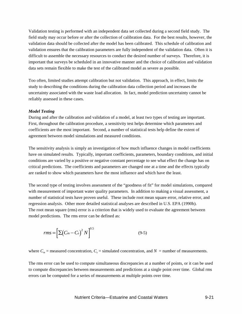
Nutrient Criteria—Estuarine and Coastal Waters 9-21
Validation testing is performed with an independent data set collected during a second field study. Thefield study may occur before or after the collection of calibration data. For the best results, however, thevalidation data should be collected after the model has been calibrated. This schedule of calibration andvalidation ensures that the calibration parameters are fully independent of the validation data. Often it isdifficult to assemble the necessary resources to conduct the desired number of surveys. Therefore, it isimportant that surveys be scheduled in an innovative manner and the choice of calibration and validationdata sets remain flexible to make the test of the calibrated model as severe as possible.
Too often, limited studies attempt calibration but not validation. This approach, in effect, limits thestudy to describing the conditions during the calibration data collection period and increases theuncertainty associated with the waste load allocation. In fact, model prediction uncertainty cannot bereliably assessed in these cases.
Model TestingDuring and after the calibration and validation of a model, at least two types of testing are important. First, throughout the calibration procedure, a sensitivity test helps determine which parameters andcoefficients are the most important. Second, a number of statistical tests help define the extent ofagreement between model simulations and measured conditions.
The sensitivity analysis is simply an investigation of how much influence changes in model coefficientshave on simulated results. Typically, important coefficients, parameters, boundary conditions, and initialconditions are varied by a positive or negative constant percentage to see what effect the change has oncritical predictions. The coefficients and parameters are changed one at a time and the effects typicallyare ranked to show which parameters have the most influence and which have the least.
The second type of testing involves assessment of the “goodness of fit” for model simulations, comparedwith measurement of important water quality parameters. In addition to making a visual assessment, anumber of statistical tests have proven useful. These include root mean square error, relative error, andregression analysis. Other more detailed statistical analyses are described in U.S. EPA (1990b).The root mean square (rms) error is a criterion that is widely used to evaluate the agreement betweenmodel predictions. The rms error can be defined as:
(9-5)( )[ ]rms C C Nm s= ∑ − 2 0.5
where Cm = measured concentration, Cs = simulated concentration, and N = number of measurements.
The rms error can be used to compute simultaneous discrepancies at a number of points, or it can be usedto compute discrepancies between measurements and predictions at a single point over time. Global rmserrors can be computed for a series of measurements at multiple points over time.

Nutrient Criteria—Estuarine and Coastal Waters9-22
When discrepancies between model simulations and measurements are not uniform over parts of theestuary or over time, the relative error may be a more appropriate statistic for testing calibration orvalidation. The relative error is defined as:
(9-6)eC C
Cm s
m=
−
where the overbars denote the average measured or simulated value. Averages can be performed overmultiple sites or over time. The relative error behaves poorly for small values of measurements ifdiscrepancies are not proportional to the magnitude of the measurement (i.e., small values of Cm magnifydiscrepancies) and if Cm > Cs (as the maximum relative error is usually taken to be 100%). Therefore, therelative error is best for computing composite statistics when discrepancies are not constant, as mayoccur when calibration over an extensive range is attempted.
Regression analysis is very useful in identifying various types of bias in predictions of dynamic-statevariables. The regression equation is written as:
(9-7)C a bCm s= + + ε
where a = intercept value, b = slope of the regression line, and = the error in measurement mean, Cm.The standard linear regression statistics computed from the above equation provide insight into thegoodness of fit for a calibration. The square of the correlation coefficient, r2, measures the percent of thevariance accounted for between measured and predicted values. The slope estimate, b, and intercept, a,can indicate any consistent biases in the model calibration. A model calibration that perfectly describedall available data would have a correlation coefficient of 1.0, a slope of 1:1, and a zero intercept.
9.5 MANAGEMENT APPLICATIONS
Once the model is calibrated and validated, it can be used to simulate future conditions to determineeffects of changes in waste loads or to investigate causes of existing problems. This section describesthree types of management application: (1) load-response analysis, (2) determination of acceptablenutrient loads, and (3) investigation of causes of nutrient problems.
Load-Response AnalysisA load-response analysis consists of performing multiple model simulations using different loading ratesand examining the water quality predicted for each simulation. The most common use of a model toinvestigate nutrients in estuaries is to determine the water quality throughout an estuary in response tochanges in nutrient loads. Models are designed to predict water quality based on loadings andenvironmental conditions (Figure 9-2).
This type of analysis also requires specification of the environmental conditions (e.g., freshwater inflows,tidal conditions) to be considered. The results of the load-response analysis are directly related to the

Nutrient Criteria—Estuarine and Coastal Waters 9-23
Figure 9-2. Use of models in load-response analysis.
environmental conditions specified for the model simulation. For example, use of summer-averageenvironmental conditions in the model will show the response in summer-average water quality tochanges in loads. For the simplest Level I models, environmental conditions are specified implicitlythrough the use of salinity observations. Predictions from these models will correspond to theenvironmental conditions that were in effect when the salinity was measured. The more complex modelsrequire explicit definition of environmental condition and can be used to provide predictions for a widerange of environmental conditions.
Acceptable Nutrient LoadsThe most common use for water quality models is to define allowable loads necessary to achieve waterquality objectives. As seen in Figure 9-2, models predict water quality for a specified set of loads andenvironmental conditions. Determination of acceptable loads typically requires an iterative procedure, asshown in Figure 9-3. The first iteration consists of performing a model simulation using existing loadsand comparing predicted water quality with objectives. Assuming that the existing loads result in unacceptable water quality, additional model simulations are performed using incremental reductions innutrient loads until water quality objectives are achieved.
The approach shown in Figure 9-3 can be used to define necessary reductions in total loads as well asreductions in individual contributors to the total load.
The results of the above approach are highly dependent on the environmental conditions selected, asallowable loading rates can vary substantially across different environmental conditions. Twoapproaches are available for selecting critical conditions for use in defining allowable loads. Theseapproaches are termed the critical conditions approach and the continuous simulation approach. In thecritical conditions approach, a single set of environmental conditions is selected for analysis. Theseconditions typically represent critical or worst-case conditions, that is, those environmental conditionsthat will result in the poorest water quality for a given set of loads. The rationale for the criticalconditions approach assumes that if loads are defined to meet water quality objectives during “critical”conditions, the same loads will result in attaining water quality objectives during most other conditions aswell.

Nutrient Criteria—Estuarine and Coastal Waters9-24
Figure 9-3. Use of models in determining allowable loads.
The continuous simulation approach performs simulations for as long a duration as is feasible, usinghistorically observed variations in environmental conditions. The predicted water quality resulting fromthe continuous simulation is analyzed to determine the frequency with which water quality problems areobserved to occur.
The overall intent of the modeling analysis is to define loads that will restrict the occurrence of waterquality problems to an acceptable frequency. Each of the above two methods has particular strengths andweaknesses for performing this task. The continuous simulation approach provides a direct means toconsider frequency of occurrence (i.e., number of years per problem) but has extreme resourcerequirements. The ability to perform continuous simulation of sufficient duration typically is constrainedby the availability of data describing historical environmental conditions, or by computationalrequirements for the higher level models. The critical conditions approach has much more manageableresource requirements; however, there are no clear methods to establish appropriate critical conditions. In estuaries, freshwater, tides, wind, and other factors all can affect water quality. Selection ofappropriate values for each environmental parameter requires considerable judgment. Furthermore, thespecific level of protection associated with any single set of environmental conditions cannot beevaluated without performing a continuous simulation.
Case Study ExampleWater quality models also can be used to gain an increased understanding of the relative importance ofvarious loading sources to an estuary or near-coastal water. It is possible to investigate the contributionof individual loading sources to the water quality problem by performing a series of simulationsexamining each loading source separately. Because most water quality models assume a linearrelationship between pollutant load and resulting water quality impact, it is possible to determine overallimpacts to the estuary by summing the impacts from each source.

Nutrient Criteria—Estuarine and Coastal Waters 9-25
13
12
11
10
9
8
7
6
5
4
3
2
1
CityWWTP
Investigation of Causes of Nutrient ProblemsShipps Creek (Figure 9-4) is a long, narrow, tidal tributary receiving nutrient inputs from upstream runoffand a single wastewater treatment plant (WWTP). This case study example demonstrates the use of models to perform three tasks:
• Estimate the contribution of various loading sources to the overall summer-average total nitrogenconcentration
• Estimate the effect of a 50% reduction in loads from the WWTP on total nitrogen concentrationsthroughout the estuary
• Estimate the reduction in loading necessary to achieve an average total nitrogen concentration of0.100 mg/L in the lower half of the estuary
Short-term answers were required, and screening-level accuracy was judged acceptable because of theshort timeframe and limited data available.
The Fraction of Freshwater Method was selected because the estuary was considered one-dimensional,long-term average results were acceptable, and the water quality target was specified in terms of totalnutrient levels.
Figure 9-4. Shipps Creek site map and salinity monitoring location.
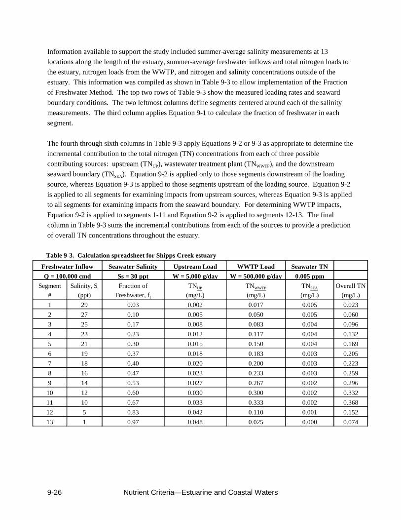
Nutrient Criteria—Estuarine and Coastal Waters9-26
Information available to support the study included summer-average salinity measurements at 13locations along the length of the estuary, summer-average freshwater inflows and total nitrogen loads tothe estuary, nitrogen loads from the WWTP, and nitrogen and salinity concentrations outside of theestuary. This information was compiled as shown in Table 9-3 to allow implementation of the Fractionof Freshwater Method. The top two rows of Table 9-3 show the measured loading rates and seawardboundary conditions. The two leftmost columns define segments centered around each of the salinitymeasurements. The third column applies Equation 9-1 to calculate the fraction of freshwater in eachsegment.
The fourth through sixth columns in Table 9-3 apply Equations 9-2 or 9-3 as appropriate to determine theincremental contribution to the total nitrogen (TN) concentrations from each of three possiblecontributing sources: upstream (TNUP), wastewater treatment plant (TNWWTP), and the downstreamseaward boundary (TNSEA). Equation 9-2 is applied only to those segments downstream of the loadingsource, whereas Equation 9-3 is applied to those segments upstream of the loading source. Equation 9-2is applied to all segments for examining impacts from upstream sources, whereas Equation 9-3 is appliedto all segments for examining impacts from the seaward boundary. For determining WWTP impacts,Equation 9-2 is applied to segments 1-11 and Equation 9-2 is applied to segments 12-13. The finalcolumn in Table 9-3 sums the incremental contributions from each of the sources to provide a predictionof overall TN concentrations throughout the estuary.
Table 9-3. Calculation spreadsheet for Shipps Creek estuary
Freshwater Inflow Seawater Salinity Upstream Load WWTP Load Seawater TNQ = 100,000 cmd Ss = 30 ppt W = 5,000 g/day W = 500,000 g/day 0.005 ppm
Segment#
Salinity, Si
(ppt)Fraction of
Freshwater, fI
TNUP
(mg/L)TNWWTP
(mg/L)TNSEA
(mg/L)Overall TN
(mg/L)1 29 0.03 0.002 0.017 0.005 0.0232 27 0.10 0.005 0.050 0.005 0.0603 25 0.17 0.008 0.083 0.004 0.0964 23 0.23 0.012 0.117 0.004 0.1325 21 0.30 0.015 0.150 0.004 0.1696 19 0.37 0.018 0.183 0.003 0.2057 18 0.40 0.020 0.200 0.003 0.2238 16 0.47 0.023 0.233 0.003 0.2599 14 0.53 0.027 0.267 0.002 0.296
10 12 0.60 0.030 0.300 0.002 0.33211 10 0.67 0.033 0.333 0.002 0.36812 5 0.83 0.042 0.110 0.001 0.15213 1 0.97 0.048 0.025 0.000 0.074

Nutrient Criteria—Estuarine and Coastal Waters 9-27
Figure 9-5. Model results for existing conditions.
The results of this modeling analysis are shown graphically in Figure 9-5, showing the overall TNdistribution as well as its component. Although the Fraction of Freshwater Method does not requirecalibration, it would be worthwhile at this point to confirm that the model predictions of TN throughoutthe estuary were consistent with observed data collected over the same time period. Figure 9-5 showsthat the WWTP is the dominant source of nitrogen throughout most of the estuary. Upstream sources arethe dominant component only at the extreme head of the estuary. Nitrogen contributions from theseaward boundary are small throughout the system. The results in Table 9-2 and Figure 9-4 satisfy thefirst objective of this study, which was to determine the contribution of various loading sources to theoverall summer-average total nitrogen concentration. The second objective of the study was to determinethe water quality resulting from a 50% reduction in WWTP TN loads. This was accomplished byreapplying Equations 9-2 and 9-3 using one-half of the original WWTP loads. Results of this analysisare shown in Figure 9-6, indicating a decrease in peak TN concentrations from 0.368 to 0.202 mg/L and adecrease in lower estuary (defined as segments 1-6) average concentrations from 0.111 to 0.064 mg/L. This nearly 50% reduction in concentrations was expected, because the original analysis haddemonstrated that the WWTP was the dominant loading source to the estuary.
The final objective of the study was to determine the loading reductions necessary to achieve a lowerestuary average concentration of 0.08 mg/L. No single answer exists to this question, because threeseparate sources of nitrogen to the estuary contribute to the total concentration. Analysis of the data inTable 9-3 shows that the incremental contribution of the upstream, WWTP, and seaward sources to lowerestuary average concentrations were 0.010, 0.100, and 0.004 mg/L, respectively. Because the seaward

Nutrient Criteria—Estuarine and Coastal Waters9-28
0.00
0.05
0.10
0.15
0.20
0.25
0.30
0.35
0.40
0.45
0.50
135791113
Segment Number
Tota
l Nitr
ogen
(mg/
l)
Total WWTP
Seaward Upstream
Figure 9-6. Model results for 50% reduction in WWTP load.
boundary nitrogen concentration cannot be controlled, management reductions must be restricted toeither the upstream sources or the WWTP. The WWTP load must be reduced by at least 20% to meet thetarget TN concentration of 0.080 mg/L; otherwise, its contribution alone will exceed the target. Beyondthe initial 20% reduction in the WWTP source, further reductions must come either from the WWTP or upstream sources. The specific allocation of these load reductions among sources is an economic andsocial decision that the model is not designed to address. The model is expressly designed, however, totest alternative proposals of load reductions to determine if they will meet the water quality objective. For example, a 25% reduction in both upstream and WWTP sources resulted in an average concentrationof 0.087 mg/L (i.e., above the target), but a 30% reduction in WWTP loads coupled with a 40%reduction in upstream loads was shown to just meet the target.
All model simulations presented here should be viewed with extreme caution, because they are based onan uncalibrated, screening-level model. The level of uncertainty for these predictions cannot bequantified and is expected to be quite large. The model results do, however, provide the best possibleestimate describing the relationship between nutrient loads and resulting concentrations, given theavailable resources.
Overview of Chesapeake Bay Airshed, Watershed, and Estuary ModelsThe cross-media models used in the Chesapeake Bay analysis consist of three models: an airshed model,a watershed model, and a model of the Chesapeake estuary. These models are linked so that the outputof one simulation provides input data for another. The simulation period is the 10-year period of January

Nutrient Criteria—Estuarine and Coastal Waters 9-29
1, 1985, to December 31, 1994. Versions of these models have been used by the Chesapeake BayProgram for more than a decade and have been refined and upgraded several times.
Airshed ModelThe Chesapeake Bay Program airshed model provides estimates of atmospheric deposition loads ofnitrogen. A product of the EPA National Exposure Research Laboratory in Research Triangle Park,North Carolina, RADM (pronounced “radum”) is an acronym for Regional Acid Deposition Model. RADM is a three-dimensional model that tracks nutrient emissions across the eastern United States. TwoRADM grids meet various resolution needs. A large grid scale covers the entire RADM domain andcontains 20,000 square cells of 6,400 square kilometers each. A fine grid scale covers the region of theChesapeake Bay watershed and has 60,000 cells, each covering 400 square kilometers. The modeldomain in the vertical is 15 cells deep, reaching from ground level to the top of the free troposphere. Thedepth of the cells increases with altitude. One of the findings of the RADM model is that the ChesapeakeBay airshed, defined as the area accounting for 75% of the deposition in the watershed, is approximately5.5 times the size of the watershed.
RADM is used to drive scenarios associated with reductions in atmospheric deposition of nitrogen. Abase condition deposition represents an estimate of the current condition of atmospheric deposition in thewatershed and is developed from a regression of National Atmospheric Deposition Program (NADP)data. RADM scenarios of atmospheric deposition reductions are incorporated into Watershed Modelscenarios by adjusting the base NADP condition on a segment-by-segment basis with a percent changeprescribed by RADM scenario results. Results from RADM specify loads of wet and dry deposition tothe Chesapeake watershed for the State Implementation Program (SIP) and Limit of Technologyscenarios. Deposition loads are input directly to the land surfaces of the watershed model or to the tidalwater surface of the Chesapeake Bay estuary model package as daily loads of wet deposition (from rainwashout of atmospheric nitrate and ammonia) and 12-year average loads of dry deposition.
Three atmospheric deposition loads were used for the Chesapeake analysis: (1) the base condition ofatmospheric deposition, (2) the estimated atmospheric deposition of nitrogen equivalent to the 1998 SIPcontrols of atmospheric deposition, and (3) the estimated atmospheric deposition under full limit oftechnology control (see Table 9-4).
Table 9-4. Chesapeake watershed nitrogen deposition under varying management schemes for emissions ofnitrogen atmospheric deposition precursors
Scenario TN Deposition (millions of kg/year)
Base Condition 204
State Implementation Plan (SIP) 178
Limit of Technology 128Sources: Chesapeake Bay Program Phase IV Watershed Model and RADM.

Nutrient Criteria—Estuarine and Coastal Waters9-30
Watershed ModelThe watershed model simulates nutrient and sediment loads delivered to the Chesapeake Bay from allareas of the watershed. Land uses of cropland, pasture, urban areas, and forests are simulated on anhourly time-step, tracing the fate and transport of input nutrient loads from atmospheric deposition,fertilizers, animal manures, and point sources. The simulation is an overall mass balance of nitrogen andphosphorus nutrients in the basin, so that the ultimate fate of input nutrients is simulated, either asincorporation into crop or forest plant material, incorporation into soil, or river runoff. Nitrogen fatesincluded volatilization into the atmosphere and denitrification. Transport in rivers is simulated to thetidal waters of the Chesapeake Bay. Sediment is simulated as eroded material washed off land surfacesand transported to the tidal bay. Scenarios are run for 10 years on a 1-hour time-step, and results areaggregated into 10-year average loads for comparison among scenarios.
To simulate the delivery of nutrients and sediment to the bay, the watershed was divided into 86 majormodel segments, each with an average area of 194,000 hectares. Segmentation, based on three tiers ofcriteria, partitioned the watershed into regions of similar characteristics. The first criterion wassegmentation of similar geographic and topographic areas, which were further delineated in terms of soiltype, soil moisture holding capacity, infiltration rates, and uniformity of slope. The second criterioninvolved finer segmentation based on spatial patterns of rainfall. Each segment had a bank-full traveltime of about 24–72 hours. The third criterion used to further delineate segments was based on featuresof the river reach. River reaches containing a reservoir were separated into a reservoir simulation and ariver simulation of the free-flowing river. For example, the James basin had 11 model segments, 2represented reservoirs on the James and Appomattox, and the segmentation generally became finer withcloser proximity to tidal waters.
Model segments were located to take advantage of observed data locations, so that a model segmentoutlet was located close to monitoring stations. Water quality and discharge data were collected fromFederal and State agencies, universities, and other organizations. More than 150 subsegments were usedat the interface between the watershed and estuary models to accurately deliver flow, nutrient, andsediment loads to appropriate areas of the estuary. Increased simulation accuracy motivated the divisionof basins into multiple segments and into simulation time-steps of an hour, but all scenario results werereported at the level of the basin and for 10-year average loads.
The watershed model has been in continuous operation at the Chesapeake Bay Program since 1982 andhas had many upgrades and refinements since that time. The watershed model used for this applicationwas Phase 4.1 based on the HSPF Version 11 code (Hydrologic Simulation Program - Fortan - HSPF). Version 11 is a widely used public domain model supported by EPA, USGS, and the U.S. Army Corps ofEngineers.
Estuary ModelThe Chesapeake Bay Estuary Model Package (CBEMP) is actually several models simulating differentaspects of water quality in the bay and tributaries. A water quality model simulates 22 parameters, orstate variables, as listed in Table 9-5.

Nutrient Criteria—Estuarine and Coastal Waters 9-31
Table 9-5. Water quality state variables used in CBEMP
Temperature Dissolved organic nitrogen
Salinity Labile particulate organic nitrogen
Inorganic suspended sediments Refractory particulate organic nitrogen
Diatoms Total phosphorus
Cyanobacteria (blue-green algae) Dissolved organic phosphorus
Other phytoplankton Labile particulate organic phosphorus
Dissolved organic carbon Refractory particulate organic phosphorus
Labile particulate organic carbon Dissolved oxygen
Refractory particulate organic carbon Chemical oxygen demand
Ammonium Dissolved silica
Nitrate + nitrite Particulate biogenic silica
Zooplankton were separated into two size classes: microzooplankton (>44 microns) andmesozooplankton (>202 microns).
Linked to the water quality model is a hydrodynamic model, simulating the hydrodynamics, or watermovement, throughout the tidal estuary. The hydrodynamic model produced three-dimensionalpredictions of velocity, diffusion, surface elevation, salinity, and temperature on an intratidal time scale. The model grid of the hydrodynamic and water quality models consists of more than 10,000 cells.
The modeling process involves simulation of living resource parameters, such as dissolved oxygen,chlorophyll concentrations, and submerged aquatic vegetation (SAV). Computed parameters arecompared with living resource standards, and an estimation is made of the degree to which computedconditions benefit the resources of interest (e.g., fish, oysters). In addition, the CBEMP includes thedirect interactive simulation of SAV and water quality. Three phytoplankton groups were simulated.
Over seasonal time scales, the bay sediments are a significant source of dissolved nutrients to theoverlying water column. The role of sediments in the systemwide nutrient budget is especially importantin summer when seasonal low flows diminish riverine nutrient input. In addition, water temperaturesenhance biological processes in the sediments, creating greater sediment oxygen demand. Bay sedimentsretain a long-term nutrient load “memory” of several years; that is, sediment nutrient fluxes to the watercolumn are determined by organic nutrient inputs from several previous years. Therefore, the waterquality model was coupled directly to a predictive benthic-sediment model. These two models interact ateach time-step, with the water quality model delivering settled organic material to the sediment bed, andthe benthic-sediment model calculating the flux of oxygen and nutrients to the water column.
Linked to the CBEMP are the watershed and airshed models, which provide daily input data. Generally,10-year scenarios are run on 15-minute time-steps with output generated each 10 days. The estuary

Nutrient Criteria—Estuarine and Coastal Waters9-32
model has been in operation since 1987, with two major model refinements released since the initial 1987steady-state model.
Further information on the entire suite of Chesapeake Bay Program models, their documentation, andapplication can be found at: http://www.chesapeakebay.net/model.htm.

Nutrient Criteria—Estuarine and Coastal Water CS-1
CASE STUDYSAN FRANCISCO BAY PROGRAM:
MANAGING COASTAL RESOURCES OF THE U.S.
The following case study is extracted from U.S. Geological Survey Fact Sheet FS-053-95 (available online at: http://water.usgs.gov/wid/html/sfb.html)
Coastal ecosystems, such as bays and estuaries, are among our most disturbed natural environments. These ecosystems also are among our most valuable habitats—estuaries supported U.S. fisheries valuedat $19 billion in 1990. Although many human activities cause change in the coastal zone, they occuragainst a background of natural change. Effective coastal-zone management requires that we identifyand understand these separate causes of ecosystem change. With this goal in mind, the United StatesGeological Survey (USGS) began in 1968 a broad program of scientific study in San Francisco Bay(Figure 1). The program is based on a conviction that sustained, multifaceted investigation of oneestuary will produce general lessons to guide the management of natural resources associated with all ourcoasts.
The USGS San Francisco Bay Program has produced more than 250 reports, including three books and areview of the human modifications of the bay. These publications are a source of guidance to resourcemanagers as they work to understand how human activities (such as water diversion, commercial trade,and waste inputs) cause change in the coastal zone. The program has been organized around themes. One of the most important themes is the integrated study of nutrients, toxic substances, and livingresources at lower levels of the food chain—the phytoplankton and bottom dwelling invertebrates. Closecollaboration between chemists and ecologists has helped to explain how plant and animal species ofcoastal ecosystems are organized into food chains, how nutrients and toxic contaminants are incorporatedinto these food chains, and how the lessons learned from detailed scientific understanding can be appliedto develop effective monitoring programs and rational environmental standards.
Nutrient EnrichmentHuman settlement around coastal water bodies has led to increased inputs of nutrients such as nitrogenand phosphorus. Many estuaries are now among the most intensively fertilized environments on Earth. Each day, San Francisco Bay receives more than 800 million gallons of municipal wastewater containing60 tons of nitrogen. In response to these concerns, the USGS developed a biological monitoringprocedure that has been used continuously since 1977 near a waste-treatment facility. Monitoringcontinued as wastewater-treatment technologies improved. This is the longest continuous record ofcontaminant concentrations in a natural environment of the United States. The transfer of monitoringprocedures developed by the USGS to local agencies and businesses serves as a model of cooperationbetween research and regulatory agencies.
Management QuestionsWater-quality managers need to know how nutrient inputs cause changes in water quality, the naturalcapacity of coastal waters to assimilate added nutrients, the level of waste treatment required to protectliving resources from the harmful effects of nutrient enrichment, and if programs of nutrient reductionare having beneficial effects.
USGS ContributionsSince 1968, the continuous study of San Francisco Bay by the USGS has given that agency a uniqueopportunity to follow ecosystem responses to improved wastewater-treatment methods as mandated byState and Federal legislation. One result of the implementation of these improved methods has been a

Nutrient Criteria—Estuarine and Coastal WaterCS-2
Figure 1. San Francisco Bay has been a focus of intensive investigation by the USGS since 1968.
large reduction in the input of ammonia-nitrogen from some municipal wastewater-treatment facilities(Figure 2).
USGS studies show that in spite of its nutrient enrichment, San Francisco Bay has not been affected byharmful algal blooms. This seeming paradox is explained partly by the abundant bottom-dwellinginvertebrates (small clams, mussels, crustaceans) that filter the water and remove new algae as fast asthey are produced. Feeding by these animals is a form of natural waste treatment that helps control thegrowth of algae in a nutrient-rich environment.
Concepts and measurement techniques from this USGS program are now incorporated into a locallyfunded and managed Regional Monitoring Program.
Lessons Learned• The chemical quality of coastal waters can respond almost immediately to waste-treatment
improvements.• Responses of biological communities to these chemical changes can take years or even decades.• Coastal water bodies have differing sensitivities to waste loading. The most cost-effective national
strategy for regulating nutrient inputs will consider these differences among ecosystems.
For Further Information:
Visit the USGS website on San Francisco Bay at: http://sfbay.wr.usgs.gov/

Nutrient Criteria—Estuarine and Coastal Water CS-3
1970 1975 1980 1985 1990 19950
5
1 0
1 5
2 0
2 5
NIT
RO
GE
N,
IN M
ILLI
GR
AM
S P
ER
LIT
ER
YEAR
CO
NC
EN
TRA
TIO
N O
F A
MM
ON
IA
S ITE 1
Figure 2. Implementation of advanced wastewater treatment in 1979 immediately reduced the input ofammonia- nitrogen to South San Francisco Bay. In prior decades, the South Bay had repeatedepisodes of oxygen depletion and animal die-offs. USGS measurements have shown acomplete cessation of these episodes since 1980. Spawning salmon have recently beenobserved in South Bay streams for the first time since the early 1900's. See figure 1 forlocation of site.

Nutrient Criteria—Estuarine and Coastal WaterCS-4
CASE STUDYLONG ISLAND SOUND - HYPOXIA
U.S. Environmental Protection Agencyhttp://www.epa.gov/region01/eco/lis/hypox.html
The ProblemDuring the summers of 1987-93, from half to two-thirds of the Sound's bottom waters experienceddissolved oxygen levels below 5 milligrams of oxygen per liter of water (mg/L). Levels of dissolvedoxygen of 5 mg/L and higher are generally accepted as being protective of the Sound's estuarine life. In1989, a particularly bad summer, more than 500 square miles (40 percent) of the Sound's bottom watershad dissolved oxygen levels less than 3 mg/L. During most of these years, dissolved oxygen in a portionof the Sound (up to 50 square miles) fell below 1 mg/L and in 1987 anoxia, the absence of any oxygen,was recorded in a portion of the Western Narrows.
These low levels of dissolved oxygen cause significant, adverse ecological effects in the bottom waterhabitats of the Sound. To date, research shows that the most severe effects (such as mortality) occurwhen dissolved oxygen levels fall below 1.5 mg/L at any time and below 3.5 mg/L in the short-term (i.e.,4 days), but that there are probably mild effects of hypoxia when dissolved oxygen levels fall below 5mg/L. The levels regularly observed in the Sound during late summer:
• Reduce the abundance and diversity of adult finfish;
• Reduce the growth rate of newly-settled lobsters and perhaps juvenile winter flounder;
• Can kill species that cannot move or move slowly, such as lobsters caught in pots and starfish, andearly life stages of species such as bay anchovy, menhaden, cunner, tautog, and sea robin;
• May reduce the resistance to disease of lobsters and other species; and
• Diminish the habitat value of Long Island Sound.
The Cause of the ProblemExcessive discharges of nitrogen, a nutrient, are the primary cause of hypoxia. Nitrogen fuels the growthof planktonic algae. The algae die, settle to the bottom of the Sound and decay, using up oxygen in theprocess.
Natural stratification of the Sound's waters occurs during the summer when warmer, fresher water"floats" on the top of cooler, saltier water that is more dense. This natural stratification forms a densitydifference between the two layers called a pycnocline. This prevents mixing of surface and bottomwaters.
Oxygen from the atmosphere and photosynthesis keep the surface layer well oxygenated, but the oxygencannot pass through the pycnocline into the bottom layer very easily. Decaying algae and other organicmaterial in the sediment and animal respiration in the bottom layer use up oxygen faster than it isreplenished. Hypoxia develops and usually persists as long as the stratification lasts (usually one to twomonths in late summer).
But hypoxia in Long Island Sound is too complex to fully understand using direct observations alone. Natural variations in weather and other physical factors affect the extent and severity of hypoxia. TheManagement Conference has constructed mathematical models in order to understand the relationship

Nutrient Criteria—Estuarine and Coastal Water CS-5
among natural variations, human-caused pollutant loadings to the Sound, and dissolved oxygen levels inthe Sound. Two models, a water quality model that approximates the biological and chemical processesof the Sound and a hydrodynamic model that describes physical processes, have been developed.
An intensive field program in Long Island Sound to collect data for the computer models was undertakenfrom April 1988 to September 1989. These data were used to calibrate and verify the models to ensurethat they reproduce the important features of the Sound. The water quality model, called LIS 2.0,provided needed insight into the causes of hypoxia and was the basis for actions to begin to reducenitrogen discharges to the Sound. However, because it simulates the movement of the Sound's waters inonly two dimensions (east-west and surface to bottom) and in a simplified manner, the LIS 2.0 model didnot provide the best technical foundation for identifying the total level of reduction in nitrogen loads thatshould be attained or the most cost-effective means to achieve targeted reductions. The hydrodynamicmodel, developed by the National Oceanic and Atmospheric Administration and completed in July, 1993,uses tide and current measurements to simulate the water's circulation in three dimensions (east-west,north-south, surface to bottom). It was coupled to the water quality model, to create LIS 3.0. The LIS 3.0model provides an advanced tool to relate sources of nitrogen from specific geographic areas to thehypoxia problem in the western Sound. Because the impact of the nitrogen load from differentmanagement zones can be deter-mined using LIS 3.0, the LISS can assign priorities for management toensure that the most the cost-effective options are pursued.
The modeling, combined with field monitoring and laboratory studies, provided a level of detail tosupport some clear conclusions about hypoxia in the Sound, its causes, and its solutions. In addition, themodels allowed the LISS to simulate water quality conditions as they were in the past, as they are today,and as they could be in the future under alternative nitrogen control scenarios.
• The most oxygen that can be dissolved in Long Island Sound at summer water temperatures isabout 7.5 milligrams per liter (mg/L) of water. This is known as the saturation level.
• Oxygen concentrations greater than 5.0 mg/L provide healthy conditions for aquatic life. Concentrations between 5.0 mg/L and 3.5 mg/L are generally healthy, except for the most sensitivespecies. When concentrations fall below 3.5 mg/L, conditions become unhealthy. The most severeeffects occur if concentrations fall below 2.0 mg/L, even for short periods of time.
• The growth of algal blooms in Long Island Sound is dependent upon the availability of nutrients. These blooms end when the pool of nitrogen available for continued growth is depleted.
• In pre-colonial days, natural, healthy biological activity brought oxygen levels below saturation dueto the natural loadings of organic material and nitrogen, but oxygen levels probably fell below 5mg/L only in limited areas and for short periods of time.
• Under today's higher nutrient and organic material loading conditions, minimum oxygen levelsaverage approximately 1.5 mg/L. These levels are associated with severe hypoxia.
• By substantially reducing nitrogen loadings to the Sound, the minimum oxygen levels in the bottomwaters during late summer can be increased to an average of about 3.5 mg/L, thereby significantlyreducing the probability and frequency of severe hypoxia and reducing the area affected byhypoxia.
• Increases in nitrogen delivered to the Sound could significantly worsen the hypoxia problem,causing larger areas to have lower oxygen levels for longer periods of time. The probability of

Nutrient Criteria—Estuarine and Coastal WaterCS-6
events like the summer of 1987, when anoxia (no oxygen) became a reality in the Sound, offshoreof Hempstead Harbor, would also increase.
Understanding the components of the load of nitrogen entering the Sound is fundamental tounderstanding the plan:
• In 1990, defined as a baseline year by the Management Conference, the total nitrogen load was90,800 tons per year.
• By 1992, the total nitrogen load had increased to 93,600 tons per year; this increase was anticipatedand was a consequence of terminating ocean disposal of sewage sludge from New York City andthe need to treat some of the sludge at facilities within the basin, reintroducing nitrogen to thewastestream.
• Of the 93,600 tons per year, approximately 39,900 tons are from natural sources and not subject toreductions by management activity.
• The remaining 53,700 tons of nitrogen per year are associated with human activities and have thepotential to be reduced through management actions.
• 10,700 tons of nitrogen per year enter the Sound through its boundaries -- the East River in the westand The Race in the east; efforts to reduce this substantial western load will come under theauspices of the New York-New Jersey Harbor Estuary Program.
• 2,200 tons of nitrogen per year enter the Sound from direct atmospheric deposition; theManagement Conference estimates that this load will be reduced to 1,540 tons of nitrogen per yearthrough implementation of the 1990 Clean Air Act amendments.
• The remaining 40,800 tons of nitrogen per year are a result of human activity coming from pointand nonpoint source discharges in the Sound's drainage basin and are the subject of the plan. Pointsource discharges, primarily sewage treatment plants, result in 32,400 tons of nitrogen each yearand nonpoint source discharges, such as agricultural and stormwater runoff, result in 8,400 tons ofnitrogen each year.
The Plan to Solve the ProblemThe goal of the hypoxia management plan is to eliminate adverse impacts of hypoxia resulting fromhuman activities. Achievement of this goal will require very large investments of capital, a long-termcommitment, and the assistance of the New York-New Jersey Harbor Estuary Program. Therefore, theManagement Conference has established interim targets for dissolved oxygen and has outlined a phasedapproach to achieving them, using what is known now to support early phases and committing to takeadditional steps as increased understanding of the environment will dictate in the future.
Interim Dissolved Oxygen TargetsUsing scientific information on the relationship between oxygen levels and ecological effects, theManagement Conference has established interim target levels for oxygen that, if achieved, wouldminimize the adverse impacts of hypoxia. In summary, the interim dissolved oxygen targets for thebottom waters of the Sound are to:

Nutrient Criteria—Estuarine and Coastal Water CS-7
• Maintain existing dissolved oxygen levels in waters that currently meet State standards;
• Increase dissolved oxygen levels to meet standards in those areas below the State standards butabove 3.5 mg/L; and,
• Increase short-term average dissolved oxygen levels to 3.5 mg/L in those areas currently below 3.5mg/L, ensuring that dissolved oxygen never goes below 1.5 mg/L at any time.
• There are also interim targets for the surface waters of the Sound.
Phased ApproachThe Management Conference is implementing a phased approach to reducing nitrogen loadings to theSound from point and nonpoint source discharges within the Sound's drainage basin.
• Phase I, as announced in December of 1990, froze nitrogen loadings to the Sound in critical areas at1990 levels to prevent hypoxia from worsening.
• Phase II, as detailed in the plan, includes significant, low-cost nitrogen reductions that begin theprocess of reducing the severity and extent of hypoxia in the Sound.
• Phase III will present nitrogen reduction targets to meet the interim targets for dissolved oxygen,which will prevent most known lethal and sublethal effects of hypoxia on the Sound's estuarine life. Phase III also will lay out the approach for meeting the nitrogen load reduction targets.
Phase I - The Nitrogen Loading FreezePhase I was announced in December 1990. It called for a freeze on point and nonpoint nitrogen loadingsto the Sound in critical areas at 1990 levels. It committed the States and local governments to specificactions to stop a 300-year trend of ever increasing amounts of nitrogen entering the Sound.
Since 1990, activities have been underway in New York and Connecticut to manage nitrogen fromsources within the New York and Connecticut portions of the drainage basin, starting with adoption ofthe Phase I “freeze” on loadings.
• Connecticut reacted quickly to obtain $15 million in State funds to ensure that the nitrogen freezewas implemented. Consent orders are in place to cap the nitrogen loads at the 15 affected facilities.
• In New York City, the New York State Department of Environmental Conservation (NYSDEC) andthe city have reached full agreement on sewage treatment permit limits, freezing total nitrogenloadings at 1990 levels.
• In Westchester County, the NYSDEC has issued final permits to the four existing sewage treatmentplants, freezing their aggregate load at the 1990 level. This was done with the full agreement of thecounty.
• On Long Island, the NYSDEC proposed individual permits that freeze the loads from individualdischarges at 1990 levels; in response, the dischargers proposed establishment of an aggregatelimit. State and local authorities agreed on aggregate load limits for targeted facilities.

Nutrient Criteria—Estuarine and Coastal WaterCS-8
Phase I agreements to control nonpoint sources centered around three categories:
• Use of existing nonpoint source and stormwater management programs to focus on nitrogen controlwith the objective of freezing the loads.
• Assessing tributary loads to Long Island Sound to begin planning for their control.
• Assigning priorities for management to coastal subbasins where nitrogen loads were estimated to bethe highest.
Phase II - Low Cost Nitrogen ReductionsFor Phase II, the LISS made a commitment in 1994 to reduce nitrogen discharges to the Sound from peakloadings by approximately 7,550 tons per year. This phase consists of incorporating a variety of low-costnitrogen removal technologies at selected sewage treatment plants. The States have moved aggressivelyto implement nitrogen control activities, using innovative strategies and seeking the cooperation of localgovernments.
In Connecticut, the goal was to achieve a reduction of 850 tons per year in nitrogen loads. The State ofConnecticut has awarded more than $15 million through its State Clean Water Fund to 11 southwesternsewage treatment plants to test and demonstrate the efficiency of upgrades for nitrogen treatment. Inaddition, the first plant in the State designed to denitrify has been constructed in Seymour. As ofDecember 1997, the load of nitrogen from plants in the Phase II agreement has been reduced by almost900 tons per year, exceeding the Phase II goal.
The State of New York revised the permits issued to sewage treatment plants, with the consent of localauthorities, to establish nitrogen limits at 1990 levels. The permits include an aggregate load forfacilities within Management Zones 7-11 (New York City, Westchester County, and Long Island). TheNew York goal was to reduce nitrogen loadings by 6,700 tons per year from peak loadings from actionsto be completed by 2006. The goal of these actions was to compensate for the increased load due tosludge treatment and reduce loadings back below 1990 levels. As of 1997, one sewage treatment plant inWestchester County and four in New York City have implemented nitrogen removal technologies. NewYork City is required to implement additional nitrogen removal technologies at the upper East Riversewage treatment plants. As of December 1997, the load of nitrogen from sewage treatment plants inNew York had decreased by 3,000 tons per year from peak loadings. In addition, New York City hasentered into a consent order to provide nitrogen removal at the reconstructed Newtown Creek facility,scheduled for completion in 2007.
In addition, both States have:
• Developed materials and conducted training for treatment plant personnel on nitrogen removaltechnologies and procedures.
• Required sewage treatment plants to identify in their plans how they will remove nitrogen, ifrequired to do so.
• Required nutrient monitoring at sewage treatment plants to improve understanding of nitrogensources and treatment plant capability.
• Increased the share of nonpoint source pollution control funds targeted to projects that reducenitrogen loads to the Sound.

Nutrient Criteria—Estuarine and Coastal Water CS-9
• Formulated Coastal Nonpoint Pollution Control Programs to address coastal nonpoint sources ofnitrogen.
• Undertaken demonstration projects that address a variety of nonpoint source control issues andtechnologies (e.g., urban runoff treatment by artificial pond/wetland systems, parking lot runofftreatment, septic system technologies to treat and remove nitrogen, controlling runoff fromagricultural land and from marinas).
As of December 31, 1997, nitrogen loadings to the Sound from point and non-point sources within theNew York and Connecticut portions of the watershed have been reduced as a result of these activities by3,900 tons per year from peak loadings.
Phase III - Nitrogen Reduction Targets to Eliminate Severe HypoxiaWhile steps taken in Phases I and II will help to reduce the extent of hypoxia, additional nitrogenreduction is needed to restore the health of Long Island Sound. Phase III sets the course by settingspecific nitrogen reduction targets for each of the 11 management zones around theSound. An array of environmental and economic considerations were taken into account throughout theprocess.
Oxygen BenchmarksThe water quality standard for oxygen in Long Island Sound is 6 mg/L in Connecticut and 5 mg/L in NewYork. Modeling indicates that even if maximum nitrogen reduction technologies were implemented, thewater quality standards for oxygen would not be achieved throughout the summer in all areas of theSound. To help establish priorities for action, the LISS has identified oxygen conditions that willminimize adverse impacts on living resources of the Sound.
Two major research efforts, a laboratory study by the EPA’s Office of Research and Development and afield study by the Connecticut Department of Environmental Protection (CTDEP) have provided much ofthe information on how low oxygen conditions affect living resources in the Sound. Both studiescorroborated that severe effects occurred whenever levels of oxygen fell below 2.0 mg/L. The fieldsurveys noted large reductions in the number and types of aquatic life present. The lab experimentsrecorded reductions in growth and increases in mortality. In both studies, effects became significantwhen oxygen levels fell below 3.5 mg/L, though some effects occurred at levels between 3.5-5.0 mg/L.
As a result, the LISS has determined that unhealthy conditions occur whenever oxygen levels fall below2.0 mg/L at any-time or remain below 3.5 mg/L over a 24-hour period. Most adverse impacts can be prevented if oxygen levels exceed these conditions, and they have been used as benchmarks to assess therelative benefits of alternative management strategies for improving the health of Long Island Sound.
Cost-effectivenessLISS managers looked at a range of nitrogen reduction options for the three major sources of nitrogen inthe watershed, sewage treatment plants, industrial facilities, and nonpoint source runoff to determine themost cost-effective option.
• Sewage Treatment Plants: As nitrogen removal requirements become more stringent, the cost ofcontrols tends to increase. To identify a cost-effective level of treatment, LISS managers arrayedthe possible nitrogen reduction options for all 70 sewage treatment plants in the 11 managementzones and calculated the average oxygen improvement in the Sound per dollar spent. Improvements at sewage treatment plants that had better than average cost-effectiveness atimproving oxygen conditions in the Sound were identified. These actions, in total, could achieve a62 percent reduction in loads, or 122,044 pounds/day.

Nutrient Criteria—Estuarine and Coastal WaterCS-10
• Industrial Facilities: A limited number of industrial facilities directly contribute nitrogen to theSound; all are located in Connecticut and contribute an estimated 6,717 pounds per day of nitrogento the Sound. Because information on the cost of reducing nitrogen from industrial sources was notreadily available, these facilities were not included in the cost analyses used for sewage treatmentplants. Instead, the cost-effective level of treatment identified for sewage treatment plants, 62percent, was applied to the industrial sources, resulting in a 4,165 pounds per day reduction forindustrial facilities. This represents an aggressive but cost-effective level of nitrogen control forthese sources.
• Nonpoint Sources: Decisions on controls of nonpoint source runoff must be made in the broadercontext of watershed management, since control measures will also help reduce suspended solids,toxic contaminants, pathogens, and floatable debris. The LISS recommends that aggressive controlsof nonpoint source pollution be implemented for both existing and new development, through bothhabitat protection and restoration activities, and structural and nonstructural best managementpractices. This effort could result in a 10 percent reduction in the non-point source load fromsources within the New York and Connecticut portions of the watershed, or 2,604 pounds per day.
Adding the potential nitrogen reductions from cost-effective controls on sewage treatment plants,industrial sources, and nonpoint runoff sources results in a total reduction of 128,813 pounds per day(23,500 tons per year). The next step is to allocate responsibility for achieving these reductions amongthe 11 management zones fairly.
Allocating ResponsibilityThe cost curve analysis provided an option for allocating nitrogen reductions among the sewagetreatment plants. Sewage treatment plant upgrades with greater than average cost-effectiveness would beimplemented while upgrades with below average cost-effectiveness would not be implemented. However, the LISS decided that relying on the cost curve analysis alone would not be a fair or evenfeasible approach and would not provide the best solution to allocating nitrogen reduction.
There are several reasons for this conclusion. Most importantly, the cost estimates were general and notuniform in their development. More accurate cost estimates must await detailed facilities planning basedupon a clear definition of the nitrogen discharge limits that will have to be met. In addition, localconcerns and considerations such as the need to purchase land for expansion and to distinguish betweencosts for nitrogen removal versus ongoing maintenance, expansions for growth, and secondary upgradeneeds (which were not included in the cost estimates) were not addressed evenly in the cost analysis.
Cost considerations aside, it is necessary for all sewage treatment plants to share the burden of nitrogenremoval. All sewage treatment plants contribute nitrogen to Long Island Sound, albeit with differenteffect. All jurisdictions will benefit from improved water quality. Therefore, it is reasonable to expectall contributors to the problem to con-tribute to the solution.
For those reasons, LISS has assigned each management zone equal responsibility to reduce its share ofthe nitrogen load. To achieve a similar level of oxygen improvement from reductions allocated to eachzone by the same percentage, the load reduction target was adjusted slightly to 23,800 tons per year fromthe original 23,500 tons per year. The total human-derived load coming from sewage treatment plants,industrial point sources, and nonpoint sources, including atmospheric depositions within the water-shed,is 40,650 tons per year. Therefore, the Soundwide nitrogen target is a 58.5 percent reduction in thehuman-derived load from point and nonpoint sources in the watershed.

Nutrient Criteria—Estuarine and Coastal Water CS-11
Phase III ActionsPhase III actions will minimize adverse impacts of hypoxia caused by human activities ina cost-effective manner, while ensuring that new information is gathered to refine and improvemanagement over the long term. Using the framework described above, the LISS set a 58.5 percentreduction target for the enriched load of nitrogen from sources within the New York and Connecticutportions of the watershed.
StrategiesAttaining the nitrogen reduction targets will require aggressive control of point sources, such as sewagetreatment plants and industrial sources, and nonpoint sources, such as on-site sewage systems and runofffrom roads, parking lots, and construction sites. To achieve the reduction targets, the States, workingwith local governments, will select the mix of point and nonpoint source controls to be implemented ineach management zone. Recognizing that each watershed is different, the plan provides the States andmunicipalities considerable flexibility in determining how nitrogen reduction actions are carried outwithin each zone.
By August 2000, the States will take the following actions:
• Develop watershed plans for each management zone that will set the course for achieving thetargets as scheduled.
• Consistent with those plans, incorporate limits on the amount of nitrogen that can be dischargedfrom sewage treatment plants and industrial sources into discharge permits.
• Conduct comprehensive nonpoint source management and habitat restoration activities.
Because the total nitrogen load entering the Sound from human sources is dominated by point sourcedischarges, the plan emphasizes technologies that can be applied to sewage treatment facilities andindustrial discharges.
In order to achieve significant reductions in the nonpoint source nitrogen load, home owners, farmers,businesses, municipalities, and the States will need to reduce current inputs of nitrogen to the watershedand restore and preserve the nitrogen removal capabilities of existing natural systems. These reductionscan be achieved using a number of approaches—resource-based land use decisions at the local level,watershed-wide use of appropriate structural and nonstructural best management practices (e.g.,stormwater detention ponds, artificial wetlands, streetsweeping, cleaning catch basins), habitat protectionand restoration, and pollution prevention management practices. All approaches will require a concertededucation and outreach effort.
TimingThe planning, financing, and construction of upgrades to sewage treatment plants necessary to achievethe 58.5 percent reduction target will require sustained effort and commitment over a long period of time. Therefore, the LISS recommends phasing-in the necessary reductions over 15 years:
• 40 percent in 5 years,
• 75 percent in 10 years, and
• 100 percent in 15 years.

Nutrient Criteria—Estuarine and Coastal WaterCS-12
CostThe Comprehensive Conservation and Management Plan identified that the cost of achieving maximumnitrogen removal from all point sources would range from $6 to $8 billion ($5.1 to $6.4 billion in NewYork State and from $900 million to $1.7 billion in Connecticut). Because of the successfuldemonstration of full scale nitrogen removal technologies at sewage treatment plants undertaken as partof Phase II, the estimated costs of capital improvements at sewage treatment plants have decreased. Theestimated cost of achieving maximum nitrogen removal levels at the 70 treatment plants in New Yorkand Connecticut is now about $2.5 billion
Because of the cost-effective approach described above, the LISS nitrogen reduction strategy would notrequire all treatment plants to meet limit-of-technology reductions. As a result, the incremental capitalcost of achieving the Phase III point source controls was estimated to be $300 million for New York Stateand $350 million for Connecticut. These cost estimates have been questioned and will be revised asmore detailed facility planning and design is performed. However, they show clearly that the potentialcost of achieving our goals can be much less than originally estimated.
Nonpoint source controls will be implemented as part of broader watershed and habitat protection efforts. The cost of controlling nonpoint sources is more difficult to estimate than the cost of point sourcecontrols. Rather than one type of technology applied to a similar source, a variety of strategies can beapplied to control a variety of nonpoint sources of nitrogen. As a result, the costs of achieving nonpointnitrogen reductions will be addressed in the zone-by-zone plans developed by the States.
FinancingAs recommended in the Comprehensive Conservation and Management Plan, the main source of fundingfor these wastewater treatment facility improvements will be the State Revolving Fund programs. TheEPA, through the federal Clean Water Act, provides financing to support State Revolving Fund loanprograms.
Connecticut uses the capitalization grant from EPA to leverage with State bond funds to provide grantsand low interest loans, at 2 percent interest over 20 years, to finance improvements at municipalfacilities. Connecticut provides about $50 million per year in State bonding to supplement the $15million per year provided under the Clean Water Act. At this capitalization rate, Connecticut should beable to meet municipal financing needs to implement Phase III nitrogen reductions. During fiscal year1997, CTDEP awarded $250 million from their Clean Water Fund to finance projects of benefit to LongIsland Sound, including major sewage treatment plant upgrades in Norwalk and Waterbury.
New York State established its State Revolving Fund in the custody of the Environmental FacilitiesCorporation. This public corporation benefits local governments in New York State by offering below-market interest rate loans to municipalities to finance wastewater improvements. Currently, the interestrate is set at up to one-half of the market rate to be repaid in 20 years. Lower rates of interest, includingzero interest loans, are available for communities that can demonstrate an inability to pay the standardsubsidized rate. Another major source of funding in New York State is the $1.75 billion CleanWater/Clean Air Bond Act approved by voters in November 1996. The Bond Act targeted $200 millionfor Long Island Sound that will be available for sewage treatment upgrades, habitat restoration, nonpointsource control, and pollution prevention.
The possible funding sources for non-point source controls reflect the diversity of both the sources andthe control options. Grant funding through federal and State water quality management, naturalresources management, and coastal zone management programs is available for nonpoint sourceactivities. The State Revolving Fund loan program is also available to fund stormwater management and

Nutrient Criteria—Estuarine and Coastal Water CS-13
habitat restoration projects but has not been used to a great extent for these types of activities due to themagnitude of existing point source funding needs in Connecticut and New York.
Effluent TradingTo provide further flexibility and incentives for maximizing the timeliness and cost-effectiveness ofnitrogen reduction actions, the LISS is investigating the feasibility of allowing effluent trading. Trading,if employed as part of the nitrogen reduction effort, may be an innovative way to use market forces tomore efficiently meet water quality goals. The LISS is developing a trading proposal and will convene apublic forum for federal, State, and local water quality officials, together with public and privateinterests, to evaluate its potential.
EnforcementThe provisions of the federal Clean Water Act provide a vehicle for ensuring that nitrogen reductiontargets are legally enforceable. Section 303(d) of the Act requires the identification of a Total MaximumDaily Load for pollutants that will result in the attainment of water quality standards. Once a TotalMaximum Daily Load has been established, the act calls for reductions to be allocated to sources so thatthe load target is met. New York and Connecticut and EPA will use their authorities to provide anenforceable foundation for achieving the nitrogen reduction targets. By August, 1998 the States willpropose a Total Maximum Daily Load designed to meet State oxygen standards. The current Long IslandSound standards were developed with limited data on how low oxygen levels affect aquatic life in LongIsland Sound. EPA is currently developing regional marine oxygen criteria that will provide a morescientifically valid basis for the development of oxygen standards. Based on this information, the Statesmay, in the future, modify their oxygen standards. While LISS managers predict significantimprovement in water quality as the nitrogen reduction targets are implemented, the attainment of currentwater quality standards at all times and in all areas is not expected. For this reason, the LISS willcontinue to assess what other kinds of actions will be needed to bring the Sound into full compliancewith water quality standards.
These actions may include control of nitrogen and carbon sources outside of the Long Island Sound basin(e.g., tributary import from point and non-point sources north of Connecticut, atmospheric deposition,boundary import from point and nonpoint sources affecting New York Harbor and The Race). Alternatives to nitrogen reduction, such as aeration, will need to be considered as a possible means toachieve water quality standards in remaining areas.
Evaluating ProgressThe LISS will track, monitor, and report on progress in meeting the nitrogen reduction targets annually.In addition, a formal review of the goals and objectives of the program will be performed every 5 years,coinciding with the progress checkpoints for nitrogen reduction. The review will consider:
• Progress and cost of implementation, including a reevaluation of the knee-of-the-curve analysisused to establish the Phase III nitrogen reduction targets,
• Improvements in technology, including the results of quality controlled pilot projects,
• The regional dissolved oxygen criteria to be published for comment,
• Water quality standards,
• Refined information on the ecosystem response to nitrogen reductions,

Nutrient Criteria—Estuarine and Coastal WaterCS-14
• The results of peer reviewed modeling, and
• Research on the impacts of hypoxia to living resources and their habitats.
Each of these factors will be considered in a balanced manner in the reevaluation process. As a result of the review, the LISS may recommend improvements that could result in changes in how the overallprogram will be implemented.
For More Information:Mark TedescoEPA Long Island Sound Office888 Washington Blvd.Stamford, CT 06904-2152Phone: 203/ 977-1541Fax: 203/ 977-1546
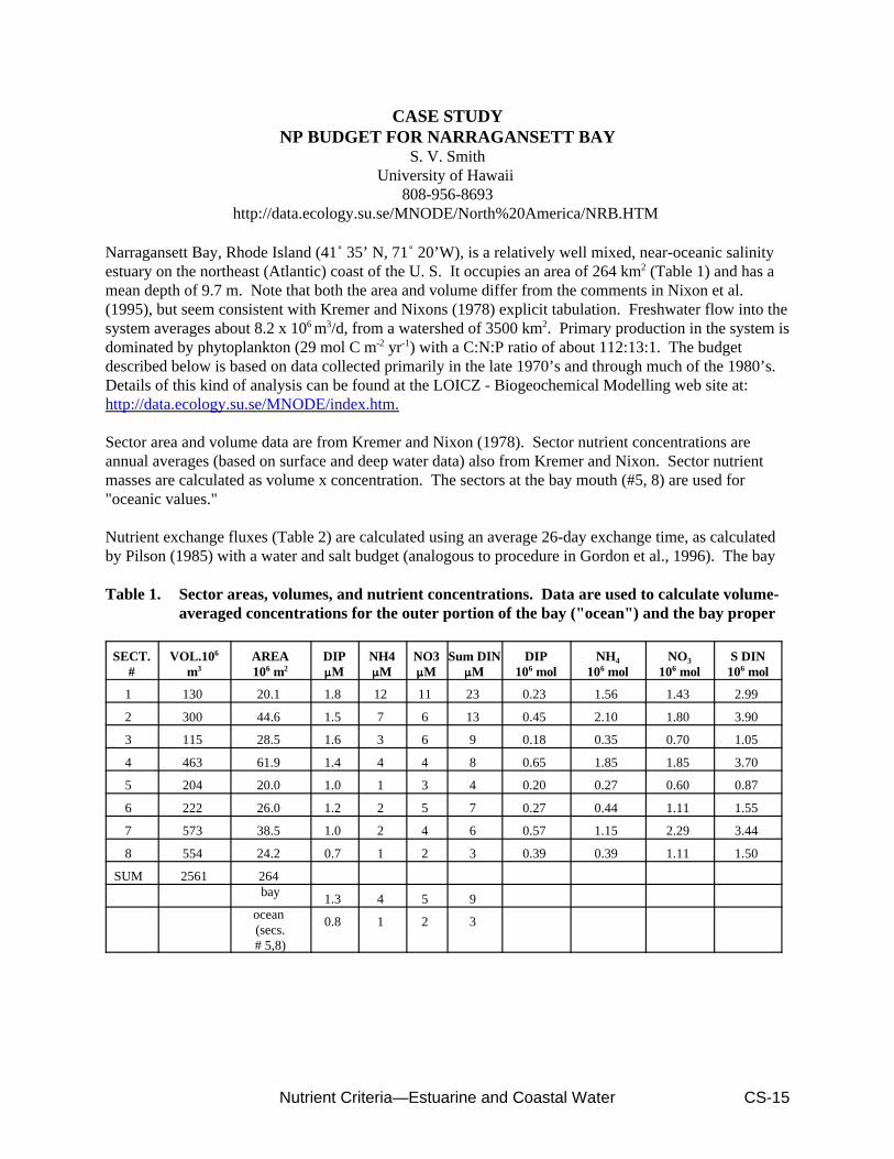
Nutrient Criteria—Estuarine and Coastal Water CS-15
CASE STUDYNP BUDGET FOR NARRAGANSETT BAY
S. V. SmithUniversity of Hawaii
808-956-8693http://data.ecology.su.se/MNODE/North%20America/NRB.HTM
Narragansett Bay, Rhode Island (41/ 35’ N, 71/ 20’W), is a relatively well mixed, near-oceanic salinityestuary on the northeast (Atlantic) coast of the U. S. It occupies an area of 264 km2 (Table 1) and has amean depth of 9.7 m. Note that both the area and volume differ from the comments in Nixon et al.(1995), but seem consistent with Kremer and Nixons (1978) explicit tabulation. Freshwater flow into thesystem averages about 8.2 x 10⁶ m3/d, from a watershed of 3500 km2. Primary production in the system isdominated by phytoplankton (29 mol C m-2 yr-1) with a C:N:P ratio of about 112:13:1. The budgetdescribed below is based on data collected primarily in the late 1970’s and through much of the 1980’s. Details of this kind of analysis can be found at the LOICZ - Biogeochemical Modelling web site at: http://data.ecology.su.se/MNODE/index.htm.
Sector area and volume data are from Kremer and Nixon (1978). Sector nutrient concentrations areannual averages (based on surface and deep water data) also from Kremer and Nixon. Sector nutrientmasses are calculated as volume x concentration. The sectors at the bay mouth (#5, 8) are used for"oceanic values."
Nutrient exchange fluxes (Table 2) are calculated using an average 26-day exchange time, as calculatedby Pilson (1985) with a water and salt budget (analogous to procedure in Gordon et al., 1996). The bay
Table 1. Sector areas, volumes, and nutrient concentrations. Data are used to calculate volume-averaged concentrations for the outer portion of the bay ("ocean") and the bay proper
SECT.#
VOL.106
m3AREA106 m2
DIP::M
NH4::M
NO3::M
Sum DIN::M
DIP106 mol
NH4
106 molNO3
106 molS DIN
106 mol
1 130 20.1 1.8 12 11 23 0.23 1.56 1.43 2.99
2 300 44.6 1.5 7 6 13 0.45 2.10 1.80 3.90
3 115 28.5 1.6 3 6 9 0.18 0.35 0.70 1.05
4 463 61.9 1.4 4 4 8 0.65 1.85 1.85 3.70
5 204 20.0 1.0 1 3 4 0.20 0.27 0.60 0.87
6 222 26.0 1.2 2 5 7 0.27 0.44 1.11 1.55
7 573 38.5 1.0 2 4 6 0.57 1.15 2.29 3.44
8 554 24.2 0.7 1 2 3 0.39 0.39 1.11 1.50
SUM 2561 264 bay 1.3 4 5 9
ocean (secs.# 5,8)
0.8 1 2 3

Nutrient Criteria—Estuarine and Coastal WaterCS-16
Table 2. Hydrographic exchange fluxes of nutrients
SOURCE OF
FLUX
DIP
106mol/yr
NH4
106mol/yr
NO3
106mol/yr
DIN
106mol/yr
residual flow -3 -7 -11 -18
net exchange flow -18 -108 -108 -216
total hydrography -21 -115 -119 -234
volume divided by the residence time gives a mixing exchange volume of 98.5 x 10⁶ m3/d, while theresidual outflow equals the freshwater inflow (i.e., 8.2 x 10⁶ m3/d). It would, in principle, be possible totime-step through the data (at monthly increments, for example). However, to do that would requirehaving the flow data to go with the nutrient data. Further, inspection of the graph by Nixon et al. (1995)of flow data and comparison of Pilson’s (1985) flow—residence time regression equation suggests thatthe residence time over this range of flow is well approximated by a constant value for the exchangetime. Various authors describe the bay as well mixed, and this is supported by the water composition datain Kremer and Nixon (1978). We therefore use a 1-box model to perform these calculations, rather thana vertically stratified model to describe hydrographic fluxes.
In Table 3, all boundary fluxes except hydrography were taken directly from by Nixon et al. (1985).Hydrographic flux was calculated as above. ) Y’s (the nonconservative fluxes) are calculated bydifference (as described in Gordon et al., 1996). No data are available for DOP, DON, or for eitherinorganic or organic C, so the budget is based on inorganic N and P only. As discussed by Gordon et al. and consistent with comments in Nixon et al., it seems safe to assume that DOP and DONnonconservative fluxes do not contribute strongly to the overall nonconservative fluxes in this system.
Rates for the D Y’s per unit area are calculated using the bay area of 264 km2 (Table 4). Note that thisarea estimate is about 25% lower than the value used by Kremer and Nixon (1978). We have used thesmaller area and volume on the basis that these are the data used to calculate the volume-averagedconcentrations. Net (nfix-denit) is calculated on the assumption that the N:P ratio of D DIP is 13:1, thenD DIN is balanced. Net (p-r) is calculated from the DIP flux, using a C:P ratio of 112:1.
Table 3. Total boundary fluxes of nutrients and inferred internal reactions—the system budget
ProcessDIP
106mol/yr
NH4
106mol/yr
NO3
106mol/yr
DIN
106mol/yr
atmosphere 0 6 19 25
rivers 13 113 177 290
urban runoff 2 13 4 17
sewage 9 136 6 142
hydrography -21 -115 -119 -234
D Y -3 -153 -87 -240
(nfix-denit) -201
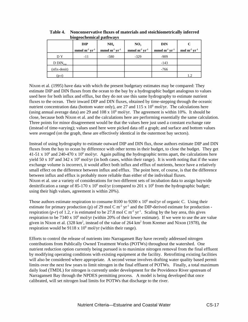
Nutrient Criteria—Estuarine and Coastal Water CS-17
Table 4. Nonconservative fluxes of materials and stoichiometrically inferredbiogeochemical pathways
DIP
mmol m-2 yr-1
NH4
mmol m-2 yr-1
NO3
mmol m-2 yr-1
DIN
mmol m-2 yr-1
C
mol m-2 yr-1
D Y -11 -580 -329 -909
D DINexp -143
(nfix-denit) -766
(p-r) 1.2
Nixon et al. (1995) have data with which the present budgetary estimates may be compared: Theyestimate DIP and DIN fluxes from the ocean to the bay by a hydrographic budget analogous to valuesused here for both influx and efflux, but they do not use this same hydrography to estimate nutrientfluxes to the ocean. Their inward DIP and DIN fluxes, obtained by time-stepping through the oceanicnutrient concentration data (bottom water only), are 27 and 115 x 106 mol/yr. The calculations here(using annual average data) are 29 and 108 x 106 mol/yr. The agreement is within 10%. It should beclose, because both Nixon et al. and the calculations here are performing essentially the same calculation. Three points for minor disagreement would be that the values here just used a constant exchange rate(instead of time-varying); values used here were picked data off a graph; and surface and bottom valueswere averaged (on the graph, these are effectively identical in the outermost bay sectors).
Instead of using hydrography to estimate outward DIP and DIN flux, those authors estimate DIP and DINfluxes from the bay to ocean by difference with other terms in their budget, to close the budget. They get41-51 x 106 and 240-470 x 106 mol/yr. Again pulling the hydrographic terms apart, the calculations hereyield 50 x 106 and 342 x 106 mol/yr (in both cases, within their range). It is worth noting that if the waterexchange volume is incorrect, it would affect both influx and efflux of nutrients, hence have a relativelysmall effect on the difference between influx and efflux. The point here, of course, is that the differencebetween influx and efflux is probably more reliable than either of the individual fluxes.Nixon et al. use a variety of considerations for two different sets of incubation data to assign baywidedenitrification a range of 85-170 x 106 mol/yr (compared to 201 x 106 from the hydrographic budget;using their high values, agreement is within 20%).
Those authors estimate respiration to consume 8100 to 9200 x 106 mol/yr of organic C. Using theirestimate for primary production (p) of 29 mol C m-2 yr-1 and the DIP-derived estimate for production -respiration (p-r) of 1.2, r is estimated to be 27.8 mol C m-2 yr-1. Scaling by the bay area, this givesrespiration to be 7340 x 106 mol/yr (within 20% of their lower estimate). If we were to use the are valuegiven in Nixon et al. (328 km2, instead of the value of 264 km2 from Kremer and Nixon (1978), therespiration would be 9118 x 106 mol/yr (within their range).
Efforts to control the release of nutrients into Narragansett Bay have recently addressed nitrogencontributions from Publically Owned Treatment Works (POTWs) throughout the watershed. Onenutrient reduction option currently being pursued is to maximize nitrogen removal from the final effluentby modifying operating conditions with existing equipment at the facility. Retrofitting existing facilitieswill also be considered where appropriate. A second venue involves drafting water quality based permitlimits over the next few years to limit nitrogen in the final effluent of POTWs. Finally, a total maximumdaily load (TMDL) for nitrogen is currently under development for the Providence River upstream ofNarragansett Bay through the NPDES permitting process. A model is being developed that oncecalibrated, will set nitrogen load limits for POTWs that discharge to the river.

Nutrient Criteria—Estuarine and Coastal WaterCS-18
For Further Information:S. V. Smith Department of Oceanography, University of Hawaii 1000 Pope Road Honolulu, Hawaii 96822 USA email: [email protected] phone: 808-956-8693 fax: 808-956-7112

Nutrient Criteria—Estuarine and Coastal Water CS-19
CASE STUDYNUTRIENT MANAGEMENT AND SEAGRASS RESTORATION IN TAMPA BAY, FLORIDA
Holly Greening, Tampa Bay Estuary Program
Abstract: Participants in the Tampa Bay Estuary Program have agreed to adopt nitrogen loadingtargets for Tampa Bay based on the water quality and related light requirements of the seagrassspecies Thalassia testudinum. Based on modeling results, it appears that light levels can bemaintained at necessary levels by “holding the line” at existing nitrogen loadings. However, thisgoal may be difficult to achieve given the 20% increase in the watershed’s human population andassociated 7% increase in nitrogen loading that are projected to occur over the next 10-20 years.
To address the long-term management of nitrogen sources, a Nitrogen Management Consortium of local electric utilities, industries and agricultural interests, as well as local governments andregulatory agency representatives, has developed a Consortium Action Plan to address the targetload reduction needed to “hold the line” at 1992-1994 levels. To date, implemented and plannedprojects collated in the Consortium Action Plan meet and exceed the agreed-upon nitrogen loadingreduction goal.
The Tampa Bay estuary is located on the eastern shore of the Gulf of Mexico in Florida, USA. At morethan 1000 km2, it is Florida’s largest open water estuary. More than 2 million people live in the 5700km2 watershed, with a 20% increase in population projected by 2010. Land use in the watershed ismixed, with about 40% of the watershed undeveloped, 35% agricultural, 16% residential, and theremaining commercial and mining.
Major habitats in the Tampa Bay estuary include mangroves, salt marshes and submerged aquaticvegetation. Each of these habitats has experienced significant areal reductions since the 1950s, due tophysical disturbance (dredge and fill operations) and water quality degradation, particularly impactingthe seagrasses due to loss of light availability. Five species of seagrass are commonly found in TampaBay, with Thalassia testudinum (turtlegrass) and Syringodium filiforme (manatee grass) dominating inthe higher salinity areas and Halodule wrightii (shoalgrass) and Ruppia maritima (widgeon grass) mostcommonly found in lower salinities.
The importance of seagrass as a critical habitat and nursery area for fish and invertebrates, and as a foodresource for manatees, sea turtles and other estuarine organisms has been recognized by the Tampa Bayresource management community for several decades. In 1990, Tampa Bay was accepted into the U.S.Environmental Protection Agency’s (EPA) National Estuary Program. The Tampa Bay National EstuaryProgram (TBNEP), a partnership that includes three regulatory agencies and six local governments, hasbuilt on the resource-based approach initiated by earlier bay management efforts. Further, it hasdeveloped water quality models to quantify linkages between nitrogen loadings and bay water quality,and models that link water quality to seagrass goals.
Recent recommendations from the National Academy of Science National Research Council (NRC)include those which regional watershed programs might consider in developing nutrient managementstrategies. The NRC recommendations are based on the process designed by the Tampa Bay EstuaryProgram partners to develop and implement a seagrass protection and restoration management programfor Tampa Bay. Critical elements of the Tampa Bay process are to:

Nutrient Criteria—Estuarine and Coastal WaterCS-20
1. Set specific, quantitative seagrass coverage goals for each bay segment.2. Determine seagrass water quality requirements and appropriate nitrogen loading targets.3. Define and implement nitrogen management strategies needed to achieve load management targets.
STEP 1. SET QUANTITATIVE RESOURCE MANAGEMENT GOALS
Establishment of clearly defined and measurable goals is crucial for a successful resource managementeffort. In 1992, TBNEP adopted an initial goal to increase current Tampa Bay seagrass cover to 95% ofthat present in 1950.
Based on digitized aerial photographic images, it was estimated that approximately 16,500 ha of seagrassexisted in Tampa Bay in 1950. At that time, seagrasses grew to depths of 1.5 m to 2 m in most areas ofthe bay. By 1992, approximately 10,400 ha of seagrass remained in Tampa Bay, a loss of more than 35%since the 1950 benchmark period. Some (about 160 ha) of the observed loss occurred as the result ofdirect habitat destruction associated with the construction of navigation channels and other dredging andfilling projects within existing seagrass meadows, and is assumed to be nonrestorable through waterquality management actions.
In 1996, the TBNEP adopted a bay-wide minimum seagrass goal of 15,400 ha. This goal represented95% of the estimated 1950 seagrass cover (minus the nonrestorable areas), and includes the protection ofthe existing 10,400 ha plus the restoration of an additional 5,000 ha.
STEP 2. DETERMINE SEAGRASS WATER QUALITY REQUIREMENTS AND APPROPRIATENITROGEN LOADING RATES
Once seagrass restoration and protection goals were established by the participants, the next stepsestablished the environmental requirements necessary to meet agreed-upon goals and subsequentmanagement actions necessary to meet those requirements.
A. Determine environmental requirements needed to meet the seagrass restoration goalRecent research indicates that the deep edges of Thalassia testudinum meadows, the primary seagrassspecies for which nitrogen loading targets are being set, correspond to the depth at which 20.5% ofsubsurface irradiance (the light that penetrates the water surface) reaches the bay bottom on an annualaverage basis. The long-term seagrass coverage goal can thus be restated as a water clarity and lightpenetration target. Therefore, in order to restore seagrass to near 1950 levels in a given bay segment,water clarity in that segment should be restored to the point that allows 20.5% of subsurface irradiance toreach the same depths that were reached in 1950.
B. Determine water clarity necessary to allow adequate light to penetrate to the 1950 seagrass deep edgesWater clarity and light penetration in Tampa Bay are affected by a number of factors, such asphytoplankton biomass, non-phytoplankton turbidity, and water color. Water color may be an importantcause of light attenuation in some bay segments; however, including color in the regression model did notproduce a significant improvement in the predictive ability of the regression model. Results of themodeling effort indicate that, on a baywide basis, variation in chlorophyll a concentration is the majorfactor affecting variation in average annual water clarity.
C. Determine chlorophyll a concentration targets necessary to maintain water clarity needed to meet theseagrass light requirementAn empirical regression model was used to estimate chlorophyll a concentrations necessary to maintainwater clarity needed for seagrass growth for each major bay segment. The adopted segment-specific
Nutrient Criteria—Estuarine and Coastal Water CS-21
annual average chlorophyll a targets (ranging from 4.6 :g/l to 13.2 :g/l) are easily measured and trackedthrough time, and are used as intermediate measures for assessing success in maintaining water qualityrequirements necessary to meet the long-term seagrass goal.
D. Determine nutrient loadings necessary to achieve and maintain the chlorophyll a targetsWater quality conditions in 1992-1994 appear to allow an annual average of more than 20.5% ofsubsurface irradiance to reach target depths (i.e., the depths to which seagrasses grew in 1950) in three ofthe four largest bay segments. Thus, a management strategy based on “holding the line” at 1992-1994nitrogen loading rates should be adequate to achieve the seagrass restoration goals in these segments. This “hold the line” approach, combined with careful monitoring of water quality and seagrass extent,was adopted by the TBNEP partnership in 1996 as its initial nitrogen load management strategy.
As an additional complicating factor, a successful adherence to the “hold the line” nitrogen loadingstrategy may be hindered by the projected population growth in the watershed. A 20% increase inpopulation, and a 7% increase in annual nitrogen load, are anticipated by the year 2010. Therefore, if theprojected loading increase (a total of 17 U.S. tons per year) is not prevented or precluded by watershedmanagement actions, the “hold the line” load management strategy will not be achieved.
STEP 3. DEFINE AND IMPLEMENT NITROGEN MANAGEMENT STRATEGIES NEEDED TOACHIEVE LOAD MANAGEMENT GOALS
Local government and agency partners in the TBNEP signed an Intergovernmental Agreement (IA) in1998 pledging to carry out specific actions needed to “hold the line” on nitrogen loadings. The IAincludes the responsibility of each partner for meeting the nitrogen management goals, and a timetablefor achieving them. How those goals are reached will be left up to the individual communities as definedby them in their Action Plans. The Tampa Bay National Estuary Program was also renamed the TampaBay Estuary Program as part of the progression from the planning phase to implementation of theadopted Comprehensive Conservation and Management Plan.
To maintain nitrogen loadings at 1992-1994 levels, local government Action Plans address that portion ofthe nitrogen target which relates to non-agricultural stormwater runoff and municipal point sourceswithin their jurisdictions, a total of 6 U.S. tons of nitrogen per year through the year 2010 (Table 1).
To address the remaining 11 U.S. tons of nitrogen of the 17 total per year each year through the year2010 needed to “hold the line” (attributed to atmospheric deposition, industrial and agricultural sourcesand springs), a Nitrogen Management Consortium of local electric utilities, industries and agriculturalinterests, as well as the local governments and regulatory agency representatives in the TBEP, wasestablished (Table 2). The Nitrogen Management Action Plan developed by public and private partnersin the Consortium combines for each bay segment all local government, agency and industry projects thatwill contribute to meeting the five year nitrogen management goal. To ensure that each partner wasusing similar nitrogen load reduction assumptions for similar projects, guidelines for calculating nitrogenload reduction credits were developed with the partners, and were used by each of the partners in thedevelopment of their action plans.
The types of nutrient reduction projects included in the Consortium’s Nitrogen Management Action Planrange from traditional nutrient reduction projects such as stormwater upgrades, industrial retrofits andagricultural best management practices to actions not primarily associated with nutrient reduction, suchas land acquisition and habitat restoration projects. A total of 105 projects submitted by localgovernments, agencies and industries are included in the Plan; 95% of these projects address nonpoint

Nutrient C
riteria—E
stuarine and Coastal W
ate
rsC
S-22
Table 1. Tampa Bay Nitrogen Management Goals
SOURCECATEGORY
CUMULATIVE 1995-1999 GOALS FOR NITROGEN REDUCTION/MANAGEMENTTOTAL
(reduction in annual load)
(tons)PinellasCounty
City ofClearwater
City of St.Petersburg
HillsboroughCounty
City ofTampa
ManateeCounty
TB Consortium*
OldTampa Bay
0.30 0.20 0.05 0.40 0.10 <0.01 1.05 2.10
HillsboroughBay
<0.01 <0.01 <0.01 4.75 8.45 <0.01 28.25 41.50
MiddleTampa Bay
<0.01 <0.01 0.90 2.50 <0.01 0.50 7.15 11.05
LowerTampa Bay
<0.01 <0.01 <0.01 <0.01 <0.01 8.35 17.00 25.35
Boca CiegaBay
0.85 <0.01 1.05 <0.01 <0.01 <0.01 2.00 3.90
TOTAL 1.15 0.20 2.00 7.65 8.55 8.85 55.45 83.85
% 1.4 0.2 2.4 9.1 10.2 10.6 66.1 100.0
* Tampa Bay Nitrogen Management Consortium

Nutrient Criteria—Estuarine and Coastal Water CS-23
Table 2. Public and Private Partners of the Tampa Bay Nitrogen ManagementConsortium, July 2001
Public Partners:
City of Tampa
City of Clearwater
City of St. Petersburg
Manatee County
Hillsborough County
Pinellas County
Manatee County Agricultural Extension Service
Environmental Protection Commission ofHillsborough County
Tampa Bay Regional Planning Council
Florida Department of Environmental Protection
Florida Fish and Wildlife Commission/FloridaMarine Research Institute
Southwest Florida Water Management District
U.S. Army Corps of Engineers
U.S. Environmental Protection Agency
Tampa Port Authority
Tampa Bay Estuary Program
Florida Department of Agriculture and ConsumerServices
Private Partners:
Florida Phosphate Council
Florida Power & Light
Tampa Electric Company
Florida Strawberry Growers Association
IMC-Phosphate
Cargill Fertilizer, Inc.
CF Industries, Inc.
Pakhoad Dry Bulk Terminals
Eastern Associated Terminals Company
CSX Transportation
sources and account for 71% of the expected total nitrogen reduction. Half (50%) of the total loadreduction will be achieved through public sector projects, and 50% by industry.
Table 3 summarizes expected reductions from those projects which were completed by the end of 1999. A total of 134 tons per year reduction in nitrogen loading to Tampa Bay is expected from the completedprojects, which exceeds the 1995-1999 reduction goal of 84 tons per year by 60%. An updated estimateof nitrogen loadings to the bay from all sources was initiated by TBEP in summer 2001, after which theeffectiveness of the proposed projects in maintaining loads to the bay will be evaluated.
Examples of specific projects and expected nitrogen loading reductions include the following:
Stormwater facilities and upgrades: Stormwater improvements or new facilities include bothpublic and private examples. Stormwater retrofits using alum injection to urban lakes reduced totalnitrogen (TN) loading by an estimated 6.4 tons per year. Stormwater improvements eliminated anestimated 2 tons of TN loading per year. Industrial stormwater improvements at phosphate

Nutrient Criteria—Estuarine and Coastal WaterCS-24
Table 3. Tampa Bay Nitrogen Management Consortium Summary of Goals and ExpectedReductions (cumulative tons TN reduced or precluded/year by the year 2000
Bay Segment
1995-1999 Nitrogen Reduction Goal
Expected Reduction: Completed or Ongoing Projects1
Expected Reduction:Atmospheric Deposition2
Old Tampa Bay 2.10 5.1 3.6 - 6.2
Hillsborough Bay 41.5 65.9 13.9 - 24.0
Middle TampaBay
11.1 21.1 4.6 - 7.9
Lower TampaBay
25.4 36.2 5.7 - 10.0
Boca Ciega Bay 3.9 5.6 1.2 - 2.1
Total 84.0 133.9 29.0- 50.2
1 Projects have been completed or are under construction. These summaries do not include reductions expected from atmosphericdeposition reductions.
2 Range of atmospheric deposition reductions expected, based on two methods.
fertilizer factories and transport terminals reduced almost 20 tons TN loading per year by the year2000.
Land acquisition and protection: Land acquisition and maintenance of natural or low intensityland uses precludes higher density uses and higher rates of TN loading. Land acquisition precludedmore than 15 tons TN loading per year by the end of 1999.
Approved overlay districts requiring additional nutrient control in management areas precluded anestimated 10 tons per year TN loading.
Wastewater reuse: Wastewater reuse programs resulted in a 6.4 ton per year reduction on TNloading. Conversion of septic systems to sewer reduced TN loading by 1.7 tons per year.
Emissions reduction: Estimated emissions reduction from coal-fired electric generating plantsbetween 1995-1997 resulted in reductions of NOx emissions of 11,700 - 20,000 tons. To estimatethe reduction of nitrogen deposition which reaches the bay (either by direct deposition to the bay’ssurface, or by deposition and transport through the watershed), a 400:1 ratio (NOx emissions unitsto nitrogen units entering the bay) is assumed. Expected reductions from atmospheric depositionthus ranged from 29 to50 tons per year by 1999. To date, emissions reductions have not beenincluded in the estimated total TN reduction to the bay, pending agreement on estimation methods.
Habitat restoration: Although typically conducted for reasons other than nutrient reduction,habitat restoration to natural land uses reduces the amount of TN loading per acre in runoff. Habitat restoration projects have been completed or are underway in all segments of Tampa Bay’swatershed. Estimated TN load reduction from completed habitat restoration projects totaled anestimated 7 tons per year.

Nutrient Criteria—Estuarine and Coastal Water CS-25
Agricultural BMPs: Water use restrictions have promoted the use of microjet or drip irrigation onrow crops (including winter vegetables and strawberries) and in citrus groves. Micro-irrigation hasresulted in potential water savings of approximately 40% or more over conventional systems and anestimated 25% decrease in fertilizer applied. Nitrogen reduction estimates from these actions total6.4 TN tons per year.
Education/public involvement: For those projects for which nitrogen load reductions have notbeen calculated or measured, but some reductions are expected, the Consortium Action Planassumes a 10% reduction estimate until more definitive information is available. These programshave reduced TN loading by an estimated 2 tons per year.
Industrial upgrades: A phosphate fertilizer mining and manufacturing plant has terminated the useof ammonia in flot-plants (an element of the fertilizer manufacturing process), resulting in areduction of 21 tons per year of nitrogen loading. Other fertilizer manufacturing companies haveupgraded their product conveyor systems, resulting in a TN reduction of more than an estimated 10tons per year due to control of fertilizer product loss. The termination of discharge by an orangejuice manufacturing plant into a tributary of Tampa Bay has resulted in a reduction of more than 11tons per year TN loading.
The approach advocated by the TBEP stresses cooperative solutions and flexible strategies to meetnitrogen management goals. This approach does not prescribe the specific types of projects that must beincluded in the Action Plan; Consortium partners have been encouraged to pursue the most cost-effectiveoptions to achieve the agreed-upon goals for nitrogen management. The TBEP will review and revisenitrogen management goals every five years, or more often if significant new information becomesavailable.
SUMMARY
The Tampa Bay management community has agreed that protection and restoration of Tampa Bay livingresources is of primary importance. Through the TBEP process (initiated in 1991), partners have adoptednitrogen loading targets for Tampa Bay based on the water quality requirements of Thalassia testudinumand other native seagrass species. A long-term goal has been adopted to achieve 15,400 ha of seagrass inTampa Bay, or 95% of that observed in 1950. To reach the long-term seagrass restoration goal, a 7%increase in nitrogen loading associated with a projected 20% increase in the watershed’s humanpopulation over the next 20 years must be offset. Government and agency partners in the Tampa BayEstuary Program and private industries and interests participating in the Nitrogen ManagementConsortium have identified and implemented specific nitrogen load reduction projects to ensure thatwater quality conditions necessary to meet long-term living resource restoration goals for Tampa Bay areachieved.
For more information:
National Research Council, National Academy of Sciences. 2000. Clean Coastal Waters:Understanding and Reducing the Effects of Nutrient Pollution. National Academy Press, Washington,D.C. 405 pages.
Janicki, A. and D. Wade. 1996. Estimating critical nitrogen loads for the Tampa Bay estuary: Anempirically based approach to setting management targets. Technical Publication 06-96 of the TampaBay National Estuary Program. Coastal Environmental, Inc., St. Petersburg, Florida.
Nutrient Criteria—Estuarine and Coastal WaterCS-26
Johansson, J.O.R. and H. Greening. 2000. Seagrass restoration in Tampa Bay: A resource-basedapproach to estuarine management. IN: Subtropical and Tropical Seagrass Management Ecology,Bortone, S. (Ed.). CRC Press, Boca Raton, FL.
Tampa Bay Estuary Program. 1998. Partnership for Progress: The Tampa Bay Nitrogen ManagementConsortium Action Plan 1995-1999. Tampa Bay Estuary Program, St. Petersburg, Florida.

Nutrient Criteria—Estuarine and Coastal Water CS-27
CASE STUDYRESTORING CHESAPEAKE BAY WATER QUALITY
Contact: Richard Batiuk, 410/267-5731; [email protected]
Original Nutrient Reduction GoalIn 1987, the Chesapeake Bay Program partners set a 40 percent reduction goal for nitrogen andphosphorus to improve low oxygen conditions in the deep trench of the mainstem bay. The goal waslater defined to apply only to “controllable” sources, and only from the States—Maryland, Virginia,Pennsylvania—and the District of Columbia are also listed as impaired tidal waters.
All listed impaired waters are scheduled to have a Total Maximum Daily Load or TMDL developed. ATMDL defines the pollutant load that a waterbody can assimilate without causing violations of waterquality standards and allocates the loading to contributing point sources and nonpoint source categories. Once a TMDL is established by a State and approved by EPA through regulatory action, it isimplemented through regulatory and nonregulatory programs. A regulatory TMDL covering the entire64,000 square mile bay watershed will be put in place by 2011 if bay water quality is not restored.
Keeping A Cooperative Approach to Bay RestorationTo avoid potential negative impacts that a regulatory TMDL process might have on the successful,cooperative efforts being used by the States’ tributary strategy programs, the Chesapeake 2000Agreement lays out a series of commitments directed toward seeking a cooperative solution to restoringbay water quality by 2010.
The bay watershed partners will define the water quality conditions necessary to support bay livingresources—fish, crabs, oyster, and bay grasses by 2001. These required conditions will be definedthrough a series of Chesapeake Bay water quality criteria for dissolved oxygen, water clarity, andchlorophyll a currently under development.
Important distinct bay and tributary tidal water habitats are being identified and characterized asdesignated uses, where the above bay criteria will be applied to fully protect the aquatic living resources.
The States with bay tidal waters—Maryland, Virginia, Delaware, and the District of Columbia—have allcommitted to adopting these bay criteria and tidal water designated uses into their individual State waterquality standards by 2003.
Critical to supporting the States’ adoption of the bay criteria and refined tidal waters designated uses willbe a baywide Use Attainability Analysis (UAA).
Loading caps on nutrients and sediments needed to meet the bay water quality criteria will be allocated tomajor tributary basins and individual States within those basins by December 2001.
Tributary strategies, detailed implementation plans to reach the allocated loading caps will be developedin cooperation with local watershed stakeholders.
A reevaluation planned for 2005 will provide an opportunity for any necessary mid-course corrections onthe road to restoring bay water quality by 2010.

Nutrient Criteria—Estuarine and Coastal WaterCS-28
Bay Criteria: Defining Restored Bay Water QualityThe Chesapeake 2000 Agreement committed the signatories to the following: “by 2001, define the waterquality conditions necessary to protect aquatic living resources.” These water quality conditions arebeing defined through the development of Chesapeake Bay specific water quality criteria for dissolvedoxygen, water clarity, and chlorophyll a. Collectively, these three water quality parameters provide thebest and most direct measures of the impacts of too much nutrient and sediment pollution on the bay’saquatic living resources—fish, crabs, oysters, and underwater bay grasses.
Bay CriteriaDissolved OxygenFish and other aquatic life require levels of dissolved oxygen to survive. Seasonal algae blooms depletedissolved oxygen, potentially rendering deep waters of the bay uninhabitable to certain species, such asthe endangered Atlantic Sturgeon during certain times of the year. Bay dissolved oxygen levels shouldbe those required by the aquatic communities inhabiting different parts of the bay during different timesof the year, fully reflective of natural conditions.
Chlorophyll aMeasurements of chlorophyll indicate levels of phytoplankton or algal biomass in the water column. Baychlorophyll levels should be moderate: not so high as to cause harmful algal blooms that lead to poorquality food, shading of light in shallow water habitats, and low dissolved oxygen conditions when thealgae die off and sink to the bottom.
Water ClarityUnderwater grasses collectively are an essential component of the bay’s living resources habitat. Decreased water clarity inhibits the growth of underwater bay grasses. Water clarity is adversely affectedby increased sediment loads and algal biomass spurred by excess nutrient inputs to the bay. Bay waterquality conditions should generally provide high water clarity—sunlight penetration—to supportrestoration of underwater grasses throughout the bay’s extensive shallow water habitats.
Chesapeake Bay Dissolved Oxygen CriteriaChesapeake Bay Dissolved Oxygen DynamicsThe Chesapeake Bay has a built-in, natural tendency toward reduced dissolved oxygen conditions,particularly within its deeper waters because of the physical morphology and estuarine circulation. Itshighly productive, shallow waters, coupled with its tendency to retain, recycle, and regenerate thenutrients delivered from the atmosphere and surrounding watershed set the stage for a nutrient-richenvironment. The mainstem Chesapeake Bay and its major tidal rivers with deep channels coming offshallower, broad shoal waters, and the significant influx of freshwater flows result in stratification of thewater column, essentially locking off deeper bottom waters from mixing with higher oxygenated surfacewaters. Combined together, the retention/efficient recycling of nutrients and water column stratificationlead to severe reductions in dissolved oxygen concentrations during the warmer months of the year,generally May to September.
Nearshore, shallow waters in the Chesapeake Bay also periodically experience episodes of low to nodissolved oxygen conditions, in part, resulting from intrusions of bottom water forced onto the shallowflanks by sustained winds (Carter et al.1978, Tyler 1984, Seilger et al.1985, Malone et al.1986). Dielcycles of low dissolved oxygen conditions often occur in nonstratified shallow waters where nighttimewater column respiration temporarily depletes dissolved oxygen levels (D’Avanzo and Kremer 1994).
The timing and spatial and volumetric extent of hypoxic and anoxic waters vary from year to year,largely driven by local weather patterns, timing and magnitude of freshwater river flow and concurrent

1 These target species were from a larger list of commercially, recreationally , and ecologically important speciesreported in Habitat Requirements for Chesapeake Bay Living Resources-Second Edition (Funderburk et al. 1991).
Nutrient Criteria—Estuarine and Coastal Water CS-29
delivery of nutrients and sediments into tidal waters, and the corresponding springtime phytoplanktonbloom (Officer et al.1984, Seliger et al.1985). In Chesapeake Bay mainstem, the onset of low to nodissolved oxygen conditions can be as early as April and persist through September, until fall turnover ofthe water column. The deeper waters of major tidal tributaries can exhibit hypoxic and anoxicconditions, with the nature, extent, and magnitude of low dissolved oxygen and the causative factorsvarying from river to river.
The scientific underpinnings of these Chesapeake Bay specific criteria have been in the works fordecades. Seasonal low dissolved oxygen conditions in the Chesapeake Bay were first documented in the1930s (Newcombe and Horne 1938). Basic understanding of dissolved oxygen dynamics, critical toderivation of criteria reflective of ecosystem process, began with the research cruises of the ChesapeakeBay Institute from the 1950s through the late 1970s. A 5-year multidisciplinary research programstarting in the late 1980s, funded by the Maryland and Virginia Sea Grant Program, yielded significantadvances in understanding of all facets of oxygen dynamics, effects, and ecosystem implications (Smithet al. 1991). These investigations laid the groundwork for more management-focused applications of thescience.
Chesapeake Bay Dissolved Oxygen Restoration GoalPublished in 1992, the Chesapeake Bay dissolved oxygen restoration goal was developed in response tothe Chesapeake Executive Council’s commitment “to develop and adopt guidelines for the protection ofwater quality and habitat conditions necessary to support the living resources found in the ChesapeakeBay system and to use these guidelines.” The dissolved oxygen restoration goal consisted of a narrativestatement supported by specific target dissolved oxygen concentrations applied over specified averagingperiods and locations. Dissolved oxygen effects information was compiled for 14 identified targetspecies1 of fish, molluscs, and crustaceans as well as for other supporting benthic and planktonic specieswithin the bay food web. The target concentrations and their specified temporal averaging and spatialapplication were determined from analysis of dissolved oxygen levels that would provide the levels ofprotection described within the narrative restoration goal. Best professional judgment was used in areaswhere there were gaps in the information base on dissolved oxygen effects available a decade ago.
The original dissolved oxygen restoration goal and its supporting framework made three breakthroughs atthat time of significance to supporting derivation and management application of the Chesapeake Bayspecific dissolved oxygen criteria within this document. The dissolved oxygen target concentrationsvaried with vertical depth through the water column as well as horizontally across the expanse of the bayand its tidal tributaries, directly reflecting variations in required levels of protection for different livingresource habitats. The averaging periods for each target concentration were tailored to specific habitats,recognizing that short-term exposures to concentrations below the target concentrations were allowableand still protective of living resources. The dissolved oxygen goal document contained a methodologythrough which water quality monitoring data and model-simulated outputs collected over varyingfrequencies could be directly assessed in terms of the percentage of time that areas of bottom habitat orvolumes of water column habitat were predicted to meet or exceed the applicable target dissolved oxygenconcentrations.
Regionalizing the EPA Virginian Province Saltwater Dissolved Oxygen CriteriaWith the publication of the EPA Ambient Water Quality Criteria for Dissolved Oxygen (Saltwater): CapeCod to Cape Hatteras came a decade’s worth of systematically developed dissolved oxygen effect dataalong with synthesis and close evaluation of several decades of effects data published in the scientific

Nutrient Criteria—Estuarine and Coastal WaterCS-30
peer reviewed literature (Thursby et al.2000). The approach to derive these dissolved oxygen criteriacombined features of the traditional water quality criteria with a new biological framework. Amathematical model was used to integrate time (replacing the concept of an averaging period) andestablish protection limits for different life stages (i.e., larvae verus juveniles and adults). Wherepractical, data were selected and analyzed in manners consistent with the Guidelines for DerivingNumerical National Water Quality Criteria for the Protection of Aquatic Organisms and Their Uses(hereafter referred to as the EPA Guidelines) (Stephan et al.1985).
The EPA Virginian Province dissolved oxygen saltwater criteria document addressed three areas ofprotection: (1) juvenile and adult survival, (2) growth effects, and (3) larval recruitment effects. In doingso, the criteria document segregated effects on juveniles and adults from those on larvae. The survivaldata on the sensitivity of the juveniles and adults are handled in a traditional EPA guidelines manner. Toaddress cumulative effects of low dissolved oxygen on larval recruitment to the juvenile life stage (i.e.,larval survival as a function of time) a new biological approach was taken. These criteria were derivedusing a mathematical model that evaluates the effect of dissolved oxygen conditions on larvae bytracking the intensity and duration of low dissolved oxygen effects across the larval recruitment season. Protection of larvae of all species is provided by using low dissolved oxygen effects data on larval stagesof nine sensitive estuarine/coastal organisms.
The Virginian Province saltwater dissolved oxygen criteria document and its underlying effects databaseand methodologies were structured to support regional specific derivation of dissolved oxygen criteriatailored to the species, habitats, and nature of dissolved oxygen exposure regimes of different estuarine,coastal, and marine waters. The segregation by life stages allows the criteria to be factored into therefined tidal water designated uses, which themselves, in part, reflect use of different habitats bydifferent life stages. This segregation by life stage is a significant difference from traditional aquatic lifecriteria.
However, the Virginian Province saltwater criteria were not explicitly set up to address natural verticalvariations in dissolved oxygen concentration. If Chesapeake Bay specific criteria were derived through astrict application of the EPA saltwater criteria methodology, there would not be the flexibility needed totailor each set of criteria to the refined tidal water designated uses. The resultant bay criteria would bedriven solely by larval effects data irrespective of depth and season.
The Chesapeake Bay specific criteria were derived through the regional application of the VirginianProvince effects database and application of traditional toxicological and new biological-based criteriaderivation methodologies. Chesapeake Bay specific science was factored directly into each step of thecriteria derivation process. The extensive Virginian Province dissolved oxygen effects database was firstfocused down on only Chesapeake Bay species and then supplemented with additional Chesapeake Bayspecies effects data from the scientific literature. The Virginian Province larval recruitment model wasmodified to better reflect Chesapeake Bay conditions, with its application broadened to includeadditional Chesapeake Bay species. Finally, specific steps were taken to factor the requirement toprovide protection of species listed as threatened/endangered in Chesapeake Bay into the bay-specificcriteria.
Current State water quality standards generally require 5 mg/L of dissolved oxygen throughout all of thebay’s waters—from the deep trench near the bay’s mouth to the shallows at the head of the bay. Eventhough the 5 mg/L standard is baywide, bay region scientists believe natural conditions dictate that insome sections of the bay, such as the deep channel, bay waters cannot achieve the current 5 mg/Lstandard during the warmer months of the year. Additionally, scientists believe other areas, such asprime migratory fish spawning areas, require higher levels of dissolved oxygen to sustain life during the

Nutrient Criteria—Estuarine and Coastal Water CS-31
38
CBP 8/9/01
CHESAPEAKE BAY PROGRAM
Dissolved Oxygen Criteria
Section 4: How Will We Define Restored Water Quality?
Minimum Amount of Oxygen (mg/L) Needed to Survive by Species
Hard Clams: 5
Striped Bass: 5-6
Worms: 1
Migratory Spawning & Nursery Areas
Shallow and Open Water Areas
Deep Water
Deep Channel
6
5
3
2
1
4
0
Crabs: 3
Spot: 2
White Perch: 5
American Shad: 5
Yellow Perch: 5
Alewife: 3.6
Bay Anchovy: 3
Figure 1. Dissolved Oxygen Criteria, Chesapeake Bay.
late winter to early summer timeframe. The amount of oxygen needed in the bay tidal waters depends onspecific needs of the aquatic living resources and where they live and during which time of the year theylive there.
The Chesapeake Bay dissolved oxygen criteria vary significantly across the five proposed tidal waterdesignated uses to fully reflect the wide array of species living in these different bay habitats (Figure 1). These working draft dissolved oxygen criteria were developed by the Chesapeake Bay Dissolved OxygenCriteria Team, a bay region team composed of scientists, State and federal managers, and technicalstakeholders (Table 1). A draft document describing the Chesapeake Bay Dissolved Oxygen Criteria ingreater detail is available for review and comment at www.chesapeakebay.net. There is a year-longprocess and schedule, including three public reviews, leading to publication of these Chesapeake Bayspecific water quality criteria by EPA by June 2002.
Chesapeake Bay Chlorophyll a CriteriaChlorophyll a is used to measure the abundance and variety of microscopic plants or algae that form thebase of the food chain in the bay. Excessive nutrients can stimulate nuisance algae blooms, resulting inreduced water clarity, reduced amount of good quality food and depleted oxygen levels in deeper water. By its very nature, chlorophyll a is both an integrated biological measure of production of the primaryfood source of the entire bay food web as well as a critical indicator of water quality through its directrole in reducing light penetration and fueling bacterial processes leading to low dissolved oxygen levels. As stated upfront by Harding and Perry (1997), “chlorophyll a is a useful expression of phytoplanktonbiomass and is arguably the single most responsive indicator of N [nitrogen] and P [phosphorus]enrichment in this system [Chesapeake Bay].” Determining the levels of chlorophyll a which are fullyprotective of the refined designated uses of the vast tidal waters that compose the Chesapeake Bay andtributaries must factor in all the different roles chlorophyll a plays in defining a restored, more balancedChesapeake Bay ecosystem.

Nutrient Criteria—Estuarine and Coastal WaterCS-32
Table 1. Working Draft Chesapeake Bay Dissolved Oxygen Criteria (July 3, 2001)
Designated Use Criteria Concentration/Duration Temporal Application
Migratory spawning andnursery
7 day mean of 6 mg/La February 15th - June 10th
Instantaneous minimum of 5 mg/L
30 day mean of 5 mg/LJune 11th - February 14th
7 day mean of 4 mg/L
Instantaneous minimum of 3.5 mg/L
Shallow/open water 30 day mean of 5 mg/L
All year round7 day mean of 4 mg/L
Instantaneous minimum of 3.5 mg/L
Deeper water 30 day mean of 3 mg/L April through September
Instantaneous minimum of 1.7 mg/L
30 day mean of 5 mg/LOctober through March
7 day mean of 4 mg/L
Instantaneous minimum of 3.5 mg/L
Deep channel
Instantaneous minimum of 1 mg/L April through September
30 day mean of 5 mg/LOctober through March
7 day mean of 4 mg/L
Instantaneous minimum of 3.5 mg/L
a Applied to tidal fresh waters with long term averaged salinities less than 0.5 parts per thousand.
The derivation of the Chesapeake Bay chlorophyll a criteria were based on the convergence of severalindependent lines of evidence—historical observed concentrations, literature values related to trophicstatus, direct contributions to light attenuation, and contribution to dissolved oxygenconditions—collaborating chlorophyll a concentrations derived as a result of characterizing set ofphytoplankton reference communities.
Phytoplankton Reference Community/Food Quality ConnectionEstimates of phytoplankton taxon biomasses were derived from the Maryland and Virginia ChesapeakeBay Monitoring Program phytoplankton count data (1984-1999) and along with other phytoplanktonindicators—chlorophyll a, pheophytin, and primary productivity—were used to investigate differences inbiomass, taxonomic composition, and food value for the range of water quality conditions currentlyexperienced in the Chesapeake Bay. The biological data were sorted into categories based on season-and salinity-specific concentrations/levels of three parameters in the associated water quality data:dissolved inorganic nitrogen, ortho-phosphate and Secchi depth. Relatively small secchi depths andexcess dissolved inorganic nitrogen and excess ortho-phosphate characterized the Poor water qualitycategories. Relatively high light levels and algal growth-limiting concentrations of dissolved inorganicnitrogen and ortho-phosphate characterized the good water quality categories. Mixed water qualityconditions (i.e., one or two water quality parameters qualified as Better but the other(s) did not) andextreme subsets of the Poor and Better categories (i.e. Worst and Best) were also investigated. Qualitative and quantitative measures of the phytoplankton community composition and biomass

Nutrient Criteria—Estuarine and Coastal Water CS-33
distributions were then evaluated relative to these water quality classifications and implications for foodquality and quantity for filter feeding fish and shellfish.
Historically Observed ConcentrationsSeveral recent in-depth reviews and evaluations of historically observed (1950s to early 1980s) andcurrent (1984-1998) chlorophyll a concentrations provide a strong basis for collaborating the ChesapeakeBay specific chlorophyll a criteria (Harding 1994, Harding and Perry 1997, Olson and Lacouture, inreview). Using information from five decades of water quality data provides insights into bothchlorophyll a concentrations that are attainable under a range of otherwise natural conditions(meteorological, river flow, tidal flushing) as well as concentrations reflective of a healthier bayecosystem.
Literature Values Related to Trophic StatusThroughout the scientific literature, there are several defining papers which through synthesis of a widearray of data from many different aquatic systems center down on ranges of conditions reflective ofdifferent trophic states of water bodies (e.g., Wetzel 1985, Ryding and Rast 1989, Smith et al.1992). Chlorophyll a is a principal parameter quantified within these literature reviews. The strength of thiscollaborative line of evidence is that information is drawn from diversity of systems across the spectrumof healthy to clearly eutrophied water bodies. This approach provides insights into commoncharacteristics associated with trophic status that can not be drawn through the study of a single, althoughlarge, water body like Chesapeake Bay.
Direct Contributions to Light AttenuationOver the past four decades, the Chesapeake Bay ecosystem has had an extensive, widely distributedunderwater grass community undergo severe declines followed by a decade and a half slow but steadyrecovery. The bay management and scientific communities have invested significant resources in theinvestigation of this grand natural experiment, learning much about the causes of the decline andpotential solutions for continued, yet accelerated restoration. Two comprehensive technical synthesizesof this wealth of scientific knowledge and insights have been published which provide direct quantitativeinsights into the role of chlorophyll a in the recovery of underwater bay grasses (Batiuk et al.1992,2000). This collaborative line of evidence draws on the chlorophyll a connection to reductions in lightpenetration through the water column.
Contribution to Dissolved Oxygen ConditionsIt is well known and documented that algae uneaten by higher trophic levels—zooplankton, oysters andfish of all kinds—becomes the fuel, through its breakdown by bacteria, for reducing dissolved oxygenlevels. Through an analysis of Chesapeake Bay water quality model simulated outputs from scenarioswhich simulated dissolved oxygen conditions which met the dissolved oxygen criteria, the modelsimulated chlorophyll a concentrations of desired dissolved oxygen conditions were quantified.
Appropriate chlorophyll a levels vary, depending on the salinity of the water. The proposed criteria forchlorophyll a are split out from tidal freshwater all the way to very salty—polyhaline—waters. Seasonof the year is also important, with spring and summer being the most important times of year that highchlorophyll a levels can impact living resources in the bay.
These working draft chlorophyll a criteria were developed by the Chesapeake Bay Chlorophyll andNutrient Criteria Team, a bay region team composed of scientists, State and federal managers, andtechnical stakeholders (Table 2). A draft document describing the Chesapeake Bay Chlorophyll aCriteria in greater detail is available for review and comment at www.chesapeakebay.net. There is a

Nutrient Criteria—Estuarine and Coastal WaterCS-34
Table 2. Working Draft Chesapeake Bay Chlorophyll a Criteria (July 3, 2001)
Salinity Regime
Chesapeake Bay Chlorophyll Criteria (ug/L)
Spring (March-May) Summer (July-September)
Median Maximum Median Maximum
Tidal Fresh 8 12 9 16
Oligohaline 10 23 6 23
Mesohaline 6 27 7 16
Polyhaline 3 7 4 9
year-long process and schedule, including three public reviews, leading to publication of theseChesapeake Bay specific water quality criteria by EPA by June 2002.
Connection to Underwater Bay GrassesThe loss of submerged aquatic vegetation, or SAV, from shallow waters of Chesapeake Bay, which wasfirst noted in the early 1960s, is a widespread, well-documented problem. Although other factors, suchas climatic events and herbicide toxicity, may have contributed to the decline of SAV in the bay, theprimary causes are eutrophication and associated reductions in light availability. The loss of SAV bedsare of particular concern because these plants create rich animal habitats that support the growth ofdiverse fish and invertebrate populations. Similar declines in SAV have been occurring worldwide withincreasing frequency during the last several decades. Many of these declines have been attributed toexcessive nutrient enrichment and decreases in light availability.
Chesapeake Bay Water Clarity Criteria
One of the major features contributing to the high productivity of Chesapeake Bay has been the historicalabundance of SAV. There are over 20 freshwater and marine species of rooted, submerged floweringplants in bay tidal waters. These underwater grasses provide food for waterfowl and are critical habitatfor shellfish and finfish. SAV also affect nutrient cycling, sediment stability, and water turbidity.
The health and survival of these plant communities in Chesapeake Bay and its tidal tributaries depend onsuitable environmental conditions that define the quality of SAV habitat. Key to the restoration of thesecritical habitats and food sources is the return of levels of light penetration in shallow waters necessary tosupport the survival, growth, and repropagation of diverse, healthy underwater bay grass communities.
Bay Water Clarity Derivation ApproachThrough the combined efforts of the bay’s scientific and resource management communities, twointernationally recognized technical syntheses of information supporting quantitative habitatrequirements for Chesapeake Bay SAV have been published in the past decade (Batiuk et al.1992, Batiuket al. 2000). Key findings, the underlying light requirements, and management-oriented diagnostic toolsand restoration targets have been reported in the peer reviewed scientific literature (Dennison et al. 1993,Kemp et al. in review; Gallegos 2001, Koch 2001, Bergstrom in preparation, Carter and Rybicki inpreparation, Karrh in preparation, Kemp et al. in preparation). These two technical syntheses ofworldwide literature, bay-specific research and field studies, and recent model simulation and dataevaluation provide the scientific foundation for the Chesapeake Bay water clarity criteria described here. Readers are encouraged to consult these two syntheses and the resultant scientific literature papers formore in-depth technical details and documentation.

Nutrient Criteria—Estuarine and Coastal Water CS-35
36
CBP 8/9/01
CHESAPEAKE BAY PROGRAM
What’s Blocking the Light?Good Water Clarity Poor Water Clarity
Algae in the water
Sediment and other particles in the water
Algae on the leaves
Percent of sunlight reaching leaves:
•9% in low salinity waters
•15% in high salinity waters
+
+
equals
Very low percentage of sunlight reaching leaves – Bay grasses grow poorly or die.
Section 4: How Will We Define Restored Water Quality?
Figure 2. Bay Water Clarity.
The Chesapeake Bay specific water clarity criteria derivation follows four successive stages: first,determination of water-column-based light requirements for SAV survival and growth, thenquantification of the factors contributing to water column light attenuation. The contributions fromepiphytes to light attenuation at the leaf surface are then factored into methods for estimating total lightattenuation. Finally, a set of minimal light requirements are determined as the actual criteria values.
The draft bay criteria propose that water clarity criteria should apply to areas of the bay that are up to 2meters deep (approximately 6 feet). Areas where SAV never occurred historically, or where naturalfactors prevent its growth (e.g., strong currents, rocky bottoms) would be excluded. The water claritycriteria reflect the different light requirements for underwater plant communities that inhabit low salinityversus higher salinity shallow water habitats throughout the bay (Figure 2).
These working draft water clarity criteria were developed by the Chesapeake Bay Water Clarity CriteriaTeam, a bay region team composed of scientists, State and federal managers, and technical stakeholders(Table 3). A draft document describing the Chesapeake Bay Water Clarity Criteria in greater detail isavailable for review and comment at www.chesapeakebay.net. There is a year-long process andschedule, including three public reviews, leading to publication of these Chesapeake Bay specific waterquality criteria by EPA by June 2002.
These Chesapeake Bay criteria will be applied to a series of designated uses which, in turn, reflect keyhabitats throughout the bay and its tidal tributaries.
Excessive Nutrient and Sediment LoadsThe causes of these water quality impairments—excessive loadings of nitrogen, phosphorus, andsediment—will be addressed through commitments to determine reductions in loadings needed toachieve the bay criteria. These required loading reductions will be established as caps on loadings

Nutrient Criteria—Estuarine and Coastal WaterCS-36
Table 3. Working Draft Chesapeake Bay Water Clarity Criteria (July 3, 2001)
Habitat Category Criteria Concentration(percent ambient light)
Temporal Application
Tidal fresh shallow water 9 % April - October
Oligohaline shallow water 9 % April - October
Mesohaline shallow water 15 % April - October
Polyhaline shallow water 15% March-May, Sept-Nov.
allocated to each tributary basin within the Chesapeake Bay watershed. This approach is consistent withEPA’s regional establishment of ambient concentration-based nutrient criteria, but places more emphasison the water quality parameters with a direct impact on aquatic living resources. Through this approachnutrients and sediments are addressed directly through caps on loading determined through application ofthe linked bay airshed-watershed-tidal water quality models and analysis of Chesapeake Bay MonitoringProgram data in place of the development of ambient nutrient and sediment criteria.
Relationship with National Efforts to Develop Nutrient CriteriaAt the same time, a parallel effort is currently underway by EPA to develop ecoregion specific numericalnutrient criteria across the country to meet the objectives of the Clean Water Action Plan. A nutrientcriteria team has been established by EPA-Region III to implement the National Nutrient Strategy issuedby EPA last year for the mid-Atlantic region. The EPA Region III team is focusing its nutrient criteriadevelopment efforts on the free flowing stream, rivers, lakes, and wetlands within the mid-AtlanticStates, not the Chesapeake Bay tidal waters. Whereas the bay criteria are focused on dissolved oxygen,water clarity and chlorophyll a, the EPA Region III team is developing ambient concentration criteria fortotal nitrogen, total phosphorus, chlorophyll, and turbidity.
The advanced scientific understanding of water quality impacts on aquatic bay living resources combinedwith the state of the art linked bay airshed-watershed -water quality models enabled the bay watershedpartners to develop criteria for water quality measures directly influencing aquatic resources. The causeof reduced water quality conditions—too much nitrogen, phosphorus, and sediment—will be addressedthrough the establishment of loading caps. The bay models enable the partners to effectively translate thedesired dissolved oxygen, water clarity, and chlorophyll a conditions back into reduced loadings ofnutrients and sediments from the surrounding watershed and airshed. Bay science has shown that it is thedelivered loads of nutrients and sediment, not just the ambient concentrations, that have had an impact onoxygen, light, and algae levels in the bay tidal waters.
Bay Tidal Water Designated UsesBecause conditions throughout the Chesapeake Bay tidal water habitats differ based on depth, salinityand season, a uniform baywide water quality standard does not take into account the varying needs ofdifferent plants and animals. As a result, current State water quality standards, which differ between thefour jurisdictions with tidal waters, need to be revised and expanded to account for the natural variabilityin conditions found throughout the bay. Each of the three bay criteria will differ from one region of thebay and its tidal tributaries to another, as determined by the plants and animals residing in that area. Once the bay criteria and the tidal water designated uses are adopted as State water quality standards,these tailored set of standards will apply to similar habitats across all jurisdictions.
An area’s designated use refers to a waterbody’s function—such as fishable or swimable—and takes intoaccount the use of the water body for public water supply, the protection of fish, shellfish, and wildlife,as well as its recreational, agricultural, industrial and navigational purposes. The existing Maryland,

Nutrient Criteria—Estuarine and Coastal Water CS-37
Refined Designated Uses forChesapeake Bay and Tidal Tributary Waters
A. Cross Section of Chesapeake Bay or Tidal Tributary
B. Oblique View of the “Chesapeake Bay” and its Tidal Tributaries
Shallow Water
Open WaterDeep Water
Deep Channel
Open WaterHabitatShallow Water
Habitat
Deep Water
Deep Channel
Migratory FinfishSpawning andNursery Habitat
Figure 3. Refined Designated Uses for Chesapeake Bay Tidal Tributary Waters.
Virginia, Delaware, and District of Columbia designated uses for the bay’s tidal waters do not fullyreflect the wide variety of different habitats found throughout the bay and its tidal tributaries. Where twojurisdictions boundaries join, each State has different designated uses for the same waterbodies.
Five refined Chesapeake Bay tidal water designated uses have been established to more fully reflect thedifferent aquatic living resource communities inhabiting a variety habitats and, therefore, the differentintended aquatic life uses of those tidal habitats (Figure 3).
The Migratory Spawning & Nursery designated use is the propagation and growth of balancedindigenous populations of ecologically, recreationally, and commercially important anadromous, semi-anadromous, and tidal fresh resident fish species inhabiting spawning and nursery grounds.
The Shallow Water designated use is the propagation and growth of balanced, indigenous populations ofecologically, recreationally, and commercially important fish, shellfish and underwater grasses inhabitingshallow waters habitats.
The Open Water designated use is the propagation and growth of balanced, indigenous populations ofecologically, recreationally, and commercially important fish, and shellfish species that inhabit openwater habitats.
The Deep Water designated use is the propagation and growth of balanced, indigenous populations ofecologically, recreationally, and commercially important fish and shellfish species inhabiting deep waterhabitats.
The Deep Channel designated use is to provide a refuge for balanced, indigenous populations ofecologically, recreationally, and commercially important fish species that depend on deep channel

Nutrient Criteria—Estuarine and Coastal WaterCS-38
UUDeep Channel
UUDeep Water
UUUUOpen Water
UUUUUUShallow Water
UUUUMigratory Spawning and Nursery
Water ClarityChlorophyll aDissolved Oxygen
Table 4. Chesapeake Bay Criteria Needed for Protection
of the Proposed Tidal Waters Designated Uses
habitats for overwintering during colder months of the year and the propagation and growth of benthicinfaunal and epifaunal worms and clams that provide food for bottom feeding fish and crabs.
These tidal water designated uses were developed by the Chesapeake Bay Water Quality StandardsCoordinators Team, a bay region team composed of water quality standards coordinators from all sixStates, the District of Columbia, EPA Region 2, 3, and headquarters offices. Table 4 shows how refinedtidal water designated uses relate to the bay criteria.
The watershed partners are evaluating the refined tidal water designated uses and the applicable baycriteria through a baywide use attainability analysis. The final tidal water designated uses will beadopted by Maryland, Virginia, Delaware, and the District of Columbia, along with the applicable baywater quality criteria into their State water quality standards by 2003. These refined designated uses willadd more specifics to the existing State designated uses and apply consistently across jurisdictions forsimilar habitats.
Baywide Use Attainability AnalysisThe Chesapeake 2000 Agreement commits the States with bay tidal waters—Maryland, Virginia, andDelaware—and the District of Columbia to adopt into their State water quality standards as consistent setof bay criteria and designated uses across bay tidal habitats. Whenever there is a proposed change inwater quality standards, such as that being undertaken for Chesapeake Bay waters, it is necessary toassess attainment of the designated uses and underlying criteria. Such an assessment is called a UseAttainability Analysis or UAA.
A UAA is used by States to justify changes to their water quality standards by assessing the physical,chemical, biological, economic, or other factors affecting attainment of the designated use. The UAAdescribes the scientific attributes of the waterbody, both natural conditions and conditions brought aboutby human contribution. If the attributes of the waterbody make attaining the use impossible, or if thereare economic reasons why the use cannot be attained, the UAA is used to clearly document these reasons. Finally, the UAA describes how the proposed standards will protect existing uses. All six bay watershedStates—New York, Pennsylvania, Maryland, Virginia, West Virginia and Delaware—along with theDistrict of Columbia and EPA are working together with bay watershed partners to carry out such an

Nutrient Criteria—Estuarine and Coastal Water CS-39
assessment. A use attainment assessment on a scale as large as the 64,000 square mile Chesapeake Baywatershed has never been carried out.
Adopting Bay Criteria as State Water Quality StandardsWater quality standards combine water quality criteria and designated uses to produce a target numericvalue assigned to a waterbody that, if achieved, will maintain healthy water quality. Through theChesapeake 2000 Agreement, Maryland, Virginia, and the District of Columbia are committed toadopting the new bay criteria–dissolved oxygen, water clarity, and chlorophyll a—along with the refinedtidal water designated uses as State water quality standards. Delaware, which shares bay tidal waterswith Maryland in its portion of the Nanticoke River watershed, has made the same commitment throughthe six-State memorandum of agreement. Together, the States and the District must achieve these newbay-specific water quality standards needed to support restored estuarine ecosystem if the ChesapeakeBay is to be removed from the list of impaired waters.
Why New State StandardsExisting State water quality standards are applied broadly across each State’s tidal waters, withoutrecognition of the variety of habitats. Each State has different water quality standards applied to thesame tidal waters, whereas the aquatic living resources in bay habitats, which do not recognize thesejurisdictional boundaries, may have the same water quality needs. Currently, dissolved oxygen is theonly numerical water quality standard adopted by all three States and the District of Columbia thataddresses nutrient- and sediment-related water quality pollution problems.
So compliance with existing State water quality standards will not fully protect the living resources in thebay waters. In some critical habitats of the bay, specifically migratory fish spawning and nursery areas,existing State water quality standards will not fully protect more sensitive life stages. In other cases,reaching existing standards is not possible owing to natural conditions found in deeper bay waters duringthe warmer months of the year. Existing State water quality standards do not include measures to protectunderwater bay grasses or fully support good quality fish food.
Setting and Allocating New Cap Loads The Chesapeake 2000 Agreement commits the signatories to determining the nutrient and sediment loadreductions necessary to achieve the water quality conditions that protect aquatic living resources. Thoseload reductions will then be assigned or allocated to each major tributary basin in the form of cap loads. Cap loads are the maximum amounts of pollutants allowed to flow into a waterbody and still ensureachievement of State water quality standards. In this case, the water quality standards will be the newbay criteria and refined tidal water designated uses (currently in draft) to be adopted by the States ofMaryland, Virginia, and Delaware, and the District of Columbia into their standards by 2003.
Available Tools and InformationThe Chesapeake Bay watershed partners will use the Chesapeake Bay Airshed, Watershed and EstuaryModels, the USGS SPARROW model, along with Chesapeake Bay Monitoring Program data, to helpdetermine these cap loads for nitrogen, phosphorus, and sediment. These models are mathematicalrepresentations that simulate the real world, interpreting various levels of actions (managementscenarios) to reduce different amounts of pollutant loads. These scenarios are run through the models todetermine how to achieve baywide attainment of the bay water quality criteria for dissolved oxygen,water clarity, and chlorophyll a as applied to the tidal water designated uses.
Cap Setting and AllocationThese models and other available information will be used to allocate loading caps to the nine majortributary basins–Susquehanna, Upper Western Shore, Patuxent, Potomac, Rappahannock, York, James,

Nutrient Criteria—Estuarine and Coastal WaterCS-40
Figure 4. The Nine Major Basins.
Upper Eastern Shore, and Virginia Eastern Shore (Figure 4). Each State and the District will bear aproportional burden for achieving and maintaining the cap based on their existing pollutant loadings,progress to date, effectiveness and cost efficiency considerations, and their pollutant loading effects ondifferent tributaries.
For multijurisdictional waters like the Susquehanna, Potomac, and Eastern Shore basins, the linkedwatershed and bay water quality models will be used to further allocate cap load responsibilities to eachState.
Working with their local stakeholders, individual States to further subdivide their major tributary basinload cap allocations into the 37 State-defined tributary strategy sub-basins.
A comprehensive 2-year schedule has been set up to coordinate the efforts of the six watershed States,the District of Columbia, and the many other involved bay watershed partners. The schedule also willensure direct and continued involvement of local stakeholders and the general public during the entirecap load setting and allocation process. The Chesapeake Bay Water Quality Steering Committee,composed of senior managers from the seven watershed jurisdictions, EPA regional and headquartersoffices, Chesapeake Bay Commission, river basin commissions, and involved stakeholders, has theoverall responsibility overseeing and reaching agreement on the cap load allocations. Many of thesubcommittees and workgroups within the Chesapeake Bay Program committee structure will be carryingout the technical, modeling, data interpretation, economic analysis, policy evaluation, andcommunication work in support of setting and allocating the nutrient and sediment cap loads.
Nutrient Criteria—Estuarine and Coastal Water CS-41
Tributary Strategies: Local Watershed Implementation The Chesapeake 2000 Agreement commits the bay watershed partners to “complete a public process todevelop and begin implementation of revised Tributary Strategies to achieve and maintain the assignedloading goals.” Tributary strategies are detailed descriptions of planned local actions—riparian forestbuffer replanting, wastewater treatment upgrades, nutrient management on farms, stormwater treatment,stream restoration, and many others—and a schedule for undertaking those actions necessary to reducenutrients and sediment loads from each tributary watershed to reach the assigned loading cap by 2010.
Development of tributary strategies has been a very driven public process with the direct involvement bylocal governments, watershed associations, regional organizations, and a wide variety of other interestedlocal stakeholders. In creating the strategies, the States, and the District of Columbia work closely withthose groups and individuals within each respective watershed who will be directly involved inimplementation strategy. Together, they explore and evaluate a wide variety of point and nonpointsource pollution control measures. They then draft a strategy using the most effective reduction optionsto achieve the cap load allocated to their tributary strategy basin.
The existing Tributary Strategies were designed to achieve the 1987 Bay Agreement goal of a 40 percentreduction in nutrient loads from controllable sources from 1985 levels. Copies of these existing tributarystrategies are available on-line through the respective Maryland, Virginia, Pennsylvania, and the Districtof Columbia tributary strategy web pages.
To restore the tidal water conditions necessary to sustain the bay’s fish, crabs, oysters and underwatergrasses will likely require greater reductions in nutrients in many areas then called for by the existingtributary strategies. In addition, the water clarity conditions needed to restore underwater bay grassescan not be achieved without significant reductions in sediments loads to the tidal waters. With NewYork, Delaware and West Virginia joining as bay watershed partners through a six-State memorandum ofunderstanding, new tributary strategies will be developed for these States’ portions of the bay watershednot previously addressed under the existing tributary strategies.
The new and revised tributary strategies will now cover all sources of nutrient and sediment pollution,including air sources, across the entire 64,000 Chesapeake Bay watershed. Tributary strategies willaddress nutrient and sediment loading caps allocated to 37 sub-basins across the bay watershed by thebay watershed partners. Loading reductions required through local stream and river segment regulatoryTMDLs will be directly integrated into each respective Tributary Strategy as part of the overall effort toeffectively “blend” the regulatory TMDL program and cooperative Chesapeake Bay Program.
Information on Local WatershedsA wide array of information is available on local watersheds within the Chesapeake Bay basin, includinginformation directly relevant to the overall process for setting and allocating new cap loads through theChesapeake Watershed Profiles. Through this point and click information system linking the baywatershed partners, one can access information on pollution sources, recent modeling results, status ofbay criteria attainment, long-term trends in water quality and living resources, draft cap allocations, andmore from the entire bay basin scale to local watersheds.
Nutrient Criteria—Estuarine and Coastal WaterCS-42
CASE STUDYA PERSPECTIVE FROM WASHINGTON STATE
Jan Newton, Washington State Department of Ecology; Randy Shuman, King County Department ofNatural Resources; Greg Pelletier, Washington State Department of Ecology
The issue of nutrient control for marine receiving waters in Washington State has its origin in a landmarkcase concerning freshwater eutrophication and lake restoration. In the early 1950's, Lake Washington, alarge lake (85 km2) situated near Seattle, Washington, was showing warning signs of ecologicaldeterioration. Following unregulated dumping of sewage from a growing urban population into the lake,classic signs of eutrophication were observed, including blooms of Oscillatoria rubescens, reduced watertransparency, and very low nitrogen to phosphorus concentration ratios. The situation was studiedextensively by Dr. W. T. Edmondson, a professor at the University of Washington, who explained thatthe changes in the lake were directly attributable to nutrient loading from sewage and wastewater(Edmondson, 1991). Edmondson made these facts known not only to the scientific community but alsoto the public and local government. The case resulted in the diversion of sewage away from the lake andis a classic example of how scientific observations and understanding were used to shape public policy. The sewage diversion and subsequent lake recovery were a success, with current day water quality of theLake far exceeding that observed during the 1950's-60's.
The solution to this classic case was to divert wastewater from Lk. Washington to nearby Puget Sound, alarge inland sea linked to the Pacific Ocean via the Strait of Juan de Fuca. Studies by Dr. G. C.Anderson, an oceanographer at the University of Washington, showed that phytoplankton in the Sound inthe vicinity of the outfall proposed to handle the diverted wastewater were limited by light and mixing,not by nutrients. Thus, diversion of effluent from the Lake to the Sound was not "shifting the problem"but rather was an ecologically sound solution. This understanding of both limnology and oceanographylaid the conceptual foundation for the formation of a large publicly funded agency (Municipality ofMetropolitan Seattle, or "Metro"). It was proposed that Metro would build a new outfall at West Point,on the Main Basin of Puget Sound, divert the sewage from Lk. Washington to West Point, and thuseliminate the nutrient enrichment problem. However, the mandate to create Metro to carry forward theseactions had to be approved in a public election first. Much controversy was associated with the processchronicled well in Edmondson's book "The Uses of Ecology" (Edmondson, 1991). Among numerouslines of objection, some public opinion maintained that Puget Sound's ecological health would bedestroyed, despite Anderson's observations. The proposed action required two election attempts before itwas approved in 1958. It is notable that the election passed before deterioration of Lk. Washington waterquality was serious; certainly the local conditions were not as serious as the symptoms seen in lakes inEurope or the Midwest North America. However, deterioration of Lk. Washington conditions didcontinue during the five years before the Metro diversion construction commenced. The persistent,dense, and obnoxious populations of Oscillatoria galvanized public opinion that the Metro diversion wasnecessary. Shortly after construction of the diversion, Lk. Washington water quality improved.
The notoriety of this event and the success of the outfall constructed at West Point to not exhibitobservable biological changes in Puget Sound resulted in widespread lore that "Puget Sound" cannot beeutrophied because the marine waters are not sensitive to nutrient addition. As Anderson's observationsimplied, the reason for the success of West Point outfall owes to the deep, well-mixed waters at the sitewhich are flushed with a residence time on the order of days. Density-driven stratification is minimal,the phytoplankton are well mixed, and any depth gradients of oxygen and nutrients do not persist. Theoutfall, at 71 m depth, diffuses effluent into water that has naturally high concentrations of nitrate andthis additional nitrogen burden is thought to not significantly contribute to phytoplankton nutrition.

Nutrient Criteria—Estuarine and Coastal Water CS-43
Ammonium concentrations in excess of normal Puget Sound background levels are observed sporadically(King County 2001) near the site and may be associated with the effluent.
This example remains well-known, but it is important to note that not all of the reaches, bays, and inletsof Puget Sound have the same characteristics of West Point and the Main Basin. Greater Puget Sound isactually composed of several basins: South Puget Sound, Hood Canal, Whidbey Basin, the Main Basin,and Admiralty Inlet with its adjoining waters with the Strait of Juan de Fuca. The first three of thesebasins have considerable freshwater-induced stratification and are much less well-flushed than the MainBasin. Residence times of these basins range weeks to months. A study funded by EPA to provide ageneral review of the state of knowledge regarding nutrient-phytoplankton relations and quantify therelative nutrient sensitivity of various areas in the Sound highlighted several areas where nutrientsbecame deplete and N:P ratios suggested nitrogen limitation (Rensel, 1991). Evidence from C-14 uptakeexperiments have shown that enhancements of primary production over ambient rates due to addednitrogen nutrient can be as high as 300% in South Hood Canal (Newton et al. 1995) and 83% in BuddInlet, located in South Puget Sound near Olympia (Newton et al. 1998). Based on environmentalattributes and human growth indicators, only a few places within Puget Sound were judged to becurrently exhibiting signs of eutrophication; however, numerous places, particularly in South Puget,Hood Canal, and Whidbey basins, were assessed to be highly susceptible to future deterioration fromeutrophication (Bricker et al. 1999).
Perhaps the first place within Puget Sound to gain wide attention for nutrient enrichment effects wassouthern Puget Sound, including Budd Inlet, Oakland Bay, Eld Inlet, Henderson Inlet, Case Inlet, andCarr Inlet. The Washington State Department of Ecology sponsored two studies in the 1980s to evaluatethe acceptability of secondary-treated wastewater discharges to marine waters in southern Puget Sound(URS, 1985, URS, 1986a). This work identified areas where new or expanded discharges wereunacceptable, based on the potential for eutrophication. A simple screening model based on effluentdilution and flushing was developed to identify the most sensitive areas.
Wastewater discharge into Budd Inlet was implicated in causing nuisance blooms of phytoplankton andadding to low dissolved oxygen concentrations noted in the bottom waters at the head of the inlet (URS,1986b). Studies sponsored by the Washington State Department of Ecology developed the firstnumerical models to relate the loading of nitrogen to phytoplankton blooms and dissolved oxygen inBudd Inlet. This work was the impetus for construction of advanced wastewater treatment systems toremove dissolved inorganic nitrogen from municipal wastewater from the regional facility that dischargesto Budd Inlet. In 1994, the wastewater entering Budd Inlet was treated for nitrogen removal. This hasresulted in substantially lower ambient nitrogen concentrations (Eisner and Newton 1997). However,regional growth continues and more capacity to process effluent is needed. Currently, theLacey-Olympia-Tumwater-Thurston County Wastewater Management Partnership (LOTT) is consideringnumerous alternatives to meet this need, including one proposal to discharge more effluent in winterwhen phytoplankton growth is minimal. LOTT undertook a large modeling and observational study: theBudd Inlet Science Study, which will be used to make the final permitting decisions.
Nutrient-induced increases to phytoplankton production with subsequent drawdown of bottom-wateroxygen has a unique character in Puget Sound relative to other North American systems because of theinfluence of upwelled Pacific Ocean water. Upwelling favorable conditions off the Washington coastlead to upwelling of deep ocean waters. These relatively low-oxygenated waters are transported in,landwards, at depth through the Strait of Juan de Fuca, as the estuarine flow of Puget Sound waters flowout, seawards, at the surface. The oceanic waters entering the Puget Sound system through AdmiraltyInlet can have oxygen concentrations as low as 5 mg/L, which then spread into the Main Basin and formthe bottom-water of the other basins as well. Seasonally low deepwater oxygen concentrations can be

Nutrient Criteria—Estuarine and Coastal WaterCS-44
found throughout Puget Sound (Newton et al., 1998; King County, 2001). Upwelling is mostlyfavorable in late summer, when productivity-related oxygen deficits are also maximal. The additivenature of human-caused eutrophication oxygen drawdown to this natural low oxygen quality, results in asmaller margin of error before deleterious effects would be noted.
The success of discharging nutrients into marine waters via regional Puget Sound wastewater plants,including the West Point facility, may be at a scale that has reached capacity. The Seattle metropolitanarea continues to grow and new Puget Sound regional wastewater facilities are needed. The King CountyCouncil recently approved that a new facility will be required to meet growth demands and is projectedfor completion in 2010. The new facility will also discharge into the Main Basin, to the north of theWest Point facility. King County is currently leading an extensive study to investigate impacts fromnutrient loading on the area. These studies include extensive water quality sampling, experiments on thesusceptibility of the waters to nutrient additions and modeling experiments to predict future impacts.
The story of nutrient control in Puget Sound continues to evolve. Ecologically sound decisions regardingnutrient management are dependent on two variables: (1) the population producing the effluent, its size,growth rate, and scale relative to the receiving waters; and (2) the sensitivity of the particular region ofthe Sound where the effluent is to be discharged to nutrients. Unfortunately, both of these attributes arehighly variable within the Puget Sound regional area, making nutrient management decisions a challengeand arguing for the utility of careful scientific studies in companion with planning efforts.

Nutrient Criteria—Estuarine and Coastal Waters A-1
APPENDIX ACONDITIONS FOR BLOOM DEVELOPMENT:
INTERPLAY AMONG BIOGEOCHEMICAL, BIOLOGICAL, AND PHYSICAL PROCESSES
OverviewIn temperate estuaries, the spring bloom typically is dominated by diatoms and occurs when freshwaterdelivers adequate amounts of N, P, and Si and other nutrients to the system. In deep estuaries, the springfreshwater inflow also provides for vertical density stratification where enough of the euphotic zoneresides near the surface to allow phytoplankton to achieve net biomass production (i.e., totalphotosynthesis minus respiration is positive). During this time solar insolation and water temperature areon the increase. For a bloom to develop, other conditions must be met. Physical flushing and localdispersion of a water parcel must be less than the doubling time for cells. Biological grazing rate mustnot be so large as to consume phytoplankton faster than cells’ doubling time.
Biogeochemical ProcessesThree aspects of N and P biogeochemistry help explain whether N or P dominates nutrient limitation inestuaries (i.e., relative nitrogen fixation rates, denitrification, and sediment regeneration of P). The firstaspect involves evidence suggesting that nitrogen fixation is less effective in marine than in freshwatersystems in making up nitrogen deficits (Howarth 1988; Schindler 1974). This finding has majorimplications for long-term coastal and open-ocean nutrient overenrichment, because N fixation is soinefficient that any balance in the N versus P limitation occurs in terms of geological time.
The second aspect involves one of the greatest differences in nutrient biogeochemical cycles betweenfreshwater and marine systems. The superior capacity of freshwater versus marine systems to retain P insediments through interactions with iron has profound implications. Nearly all the P deposited in marinesediments is remineralized annually (Caraco et al. 1990) and depends heavily on the sulfateconcentration, which can be used as a surrogate for salinity. Thus, P in freshwater sediments is boundmore tightly, and proportionally less is released back into the water column. Also, P release from marinesediments is temperature dependent, and its maximum release during the summer helps explain thetendency for increasing water column concentrations of P to occur during that season in many estuaries(Nixon et al. 1980). Estuaries with a well-developed tidal freshwater zone might be expected to be moreP-limited than estuarine systems with small tidal fresh areas.
More details on nutrient cycling in subtropical and tropical marine waters, systems much less studiedthan northern temperate estuaries, are provided by Bianchi et al. (1999). The extensive coastal wetlandsystems (e.g., marshes and mangroves) that border the Gulf of Mexico provide environments wherechemical transformations and storage of nutrients occur. Also, extensive seagrass meadows apparentlytie up inorganic N and P so that relatively less remains free in the water column. In general, DIN andPO4 concentrations are much lower in northern Gulf river-dominated estuaries (e.g., Mobile andApalachicola Bays) than similar U.S. East Coast systems, presumably because of the lower point sources. Local groundwater sources are important and water quality managers should be aware of them. However, local estuarine point sources of N and P may alter nonpoint source patterns (e.g., paper millsand wastewater treatment facilities) (Livingston 2001a).
Denitrification is the third aspect that plays a role in N limitation in estuaries and coastal waters (Nixonet al. 1996). Denitrification is the process whereby nitrate is converted to gaseous N2 and N2O andthereby made unavailable. Denitrification provides a sink for N in estuarine systems. Shelf watersgenerally are too deep to provide enough sediment-water column contact for a quantitatively significantmagnitude of denitrification to occur. Bottom-water anoxia limits nitrification and hence denitrification

Nutrient Criteria—Estuarine and Coastal WatersA-2
in the high-sulfide sediments where nitrification and denitrification are coupled (Jenkins and Kemp1984). Knowledge of the magnitude of denitrification can help the water quality manager predict thenutrient overenrichment response of an estuary, because N that is denitrified is largely unavailable tosupport primary production.
Biological ProcessesThe relative importance of biological grazing should be assessed, because when a nutrient problemoccurs it is evidence that enrichment has exceeded the ability of the system to maintain a steady state innet biomass production at pre-enrichment levels. For example, major changes in the biology of estuariesin terms of particle filtering capacity (e.g., oysters: Newell 1988) and probably filter feeding finfish (e.g., menhaden) can modify phytoplankton primary production, although the quantitative effectiveness of suchcropping is scientifically unsettled. Nutrient overenrichment may drive marine waters toward smalleralgae and other microbes (Jonas 1992) where organic carbon flows more to the microbial loop (Hassett etal. 1997), versus more direct flow to copepods and higher trophic levels (e.g., finfish). This shift in thefood web may be a significant factor in how estuaries “assimilate” increased nutrient inputs (Roelke et al.1999; Roelke 2000).
Physical Processes and FactorsConceptual FrameworkSmith (1984) argued that there is no inherent difference in nutrient limitation between lakes and theocean. Abundant evidence indicates that phytoplankton net primary production in north temperate lakestends to be P limited, and phytoplankton production in the ocean as a whole is potentially moderately Plimited but at higher P concentrations than lakes. This conclusion is supported by the observation thatTN:TP ratios of the surface ocean are usually well in excess of the Redfield ratio (Guildford and Hecky2000). Local deviations have been detected. In contrast to lakes and oceans, estuaries and coastal shelfwaters tend to be N limited, with some exceptions. Water quality managers may question the reason forthis, as the three case studies described earlier, especially temperate estuaries and the coastal shelf,appear to be N limited and not P limited. Such an understanding is basic to arguments about cause andeffect and also what ecosystem conditions drive a coastal ecosystem toward N limitation or P limitation. Smith provided an explanation that still has merit.
Smith posited that the apparent difference in limiting nutrient between lakes and oceans lies, in part, withthe relative rates for material exchange via physical processes of advection (i.e., transport of water andassociated constituents) and eddy diffusion (i.e., local transport of material against a concentrationgradient) and biogeochemical processes of N fixation and fixed N loss. The argument is based on fieldexperiments in marine embayments with little or no freshwater input, so advective transport of nutrientsfrom the land simplified nutrient budget development. Smith postulates that if the physical exchangerates are long (e.g., open ocean), then the system would tend toward P limitation because biogeochemicaladjustment of the N:P availability ratio is short compared with long physical exchange rates (e.g., monthsto a year or longer). In other words, nitrogen fixation would balance any losses of nitrogen associatedwith phytoplankton sedimentation, but P has no atmospheric reservoir or biochemical mechanism for anequivalent P fixation to occur. If the physical exchange rates are faster than biochemical rates (e.g.,nitrogen fixation), then net ecosystem production (and by inference net phytoplankton biomassproduction) of organic material may be N limited; if the biochemical rates are faster, then net productionwill tend toward P limitation. The ratio of the residence time of the water to the biogeochemical turnoverrate indicates the degree to which the hydrodynamic processes dominate or modify estuarine ecosystems(Day et al. 1989). This is an example of the importance of scaling critical processes (Harris 1986). Smith’s conceptual model should apply to estuaries and shelf waters. Smith’s data, analysis, andsynthesis and other empirical data support N limitation in estuaries and coastal shelf environments.

Nutrient Criteria—Estuarine and Coastal Waters A-3
Figure A-1. Scales of phytoplankton ecology. Horizontal and vertical scalesare determined by the respective diffusion coefficients Kh and KL. The timescales for the algae are determined by the scales of growth (shaded band). Theprocesses of importance at each scale are noted. In the past it was alwaysassumed (wrongly) that physiological processes were at equilibrium and thatclimatological variability could be ignored. Source: Harris 1986.
The concept of scale is another element of the conceptual framework. Physical processes that modify theexpression of bloom dynamics will best be detected at the ecological level (Figures A-1, A-2). In thiscontext, Geyer et al. (2000) cite many examples supporting the observation that “at virtually everyspatial scale, within every component of estuarine ecosystems, physical processes influence thedistribution and fate of chemicals (sic including nutrients) and organisms.” Physical processes areinvolved in the delivery of nutrients to the biota in estuaries and coastal shelf waters, and alsofundamentally influence advective and dispersive processes that transport and retain dissolved andparticulate material, including nutrients and plankton in estuaries and on the coastal shelves. The roles ofphysical processes influencing net biomass production of phytoplankton are explored in the main text inmore detail.

Nutrient Criteria—Estuarine and Coastal WatersA-4
Figure A-2. The left panel shows the distribution of chlorophyll—an indicator of algal biomass—along the eastcoast of the U.S. from Boston to South Carolina as measured from the ocean color satellite SeaWIFs. Note thehigher chlorphyll levels closer to shore, and the much higher levels in enclosed bays, such as Pamlico Sound(latitude 35°) and Chesapeake Bay (mouth at 37° latitude). The above panel shows chlorophyll distributions withinChesapeake Bay in more detail, as measured during a phytoplankton bloom. Both images were taken in April 1998. Source: Howarth et al. 2000.

Nutrient Criteria—Estuarine and Coastal Waters B-1
APPENDIX BADDITIONAL INFORMATION ON THE ROLE OF TEMPERATURE AND LIGHT
ON ESTUARINE AND COASTAL MARINE PHYTOPLANKTON
Availability in temperature and light values can be plotted as hydroclimographs (e.g., polygons) topicture their relative seasonal change around the coasts. A temperature increase will lower the density ofseawater and contribute to density stratification. In particular, rapid changes in water temperatureinfluence the rate of biological metabolic processes, including algal growth rates (Eppley 1972). Somespecies exhibit various degrees of thermal adaptation when temperature changes are gradual.
Speculation suggests that if sea temperatures continue to rise as a function of the “greenhouse effect,”estuarine biotic communities may change over the next several decades as they approach thermal limits. For example, although the seagrasses Halodule (shoalgrass) and Zostera (eelgrass) now overlap in CoreSound, NC, a northward migration of Halodule and a retreat of Zostera may occur if water temperaturesrise faster than populations can adapt. Such relationships and their potential alteration probably can bedocumented for other biotic groups along other coasts. For example, if temperature now limits regularflowering of the seagrass Thalassia (turtle grass) along the northern Gulf of Mexico, then increasedflowering may occur if temperatures warm. Such conjectures notwithstanding, however, littleinformation is available to help assess the consequences of a potential interaction between an increasedtemperature rise and increased nutrient supply on seagrasses.
Light has a fundamental role in aquatic primary production and is essential in the development of modelsto estimate phytoplankton primary production (Behrenfeld and Falkowski 1997) and submerged aquaticvegetation (Dennison et al. 1993). Many concepts in aquatic ecology are based on the light gradient(Huisman 1999) (e.g., diel plankton vertical migration, benthic animals migrating out of sediments, depthof euphotic zone, and mixing depth). Phytoplankton growth, nutrient relationships, light, and otherphysical processes interact in a feedback system. Although light may be adequate and all otherrequirements met for their formation, blooms may not form if dispersive processes are greater than algalcell doubling time (Kierstead and Slobodkin 1953; Lucas et al. 1999). Tidal ranges greater thanapproximately 2.0 m apparently disperse phytoplankton faster than cell doubling time, even if nutrientconditions would be supportive of a bloom (Monbet 1992).
Both the vertical distribution of phytoplankton abundance and community composition are frequentlychanging in the water column. Swimming through use of a flagellum, especially by dinoflagellates, andchanges in cell density through physiological mechanisms allow modest vertical mobility against weakmixing forces. If the mixing depth is substantially greater than the euphotic zone depth (e.g., a depthwhere approximately 1% of surface insolation occurs), then phytoplankton spend too much time in aninadequate light environment and net primary production is limited (Figure B-1) (Huisman et al. 1999). The compensation depth is where water column phytoplankton photosynthesis and respiration are inbalance, and this often approximates the 1% insolation depth, or about two times the Secchi disc depth(Parsons and Takahashi 1973). For example, in the lower Delaware Bay the upper-mixed layer oftencorresponds to the bay bottom, the result of which is that phytoplankton spend too much time below thecompensation depth and hence low biomass production occurs (Pennock 1985). In systems where thedominant support of the food web is derived from photosynthesis, net phytoplankton production must belarge enough to support the microbial loop (Azam et al. 1983) and higher trophic levels.
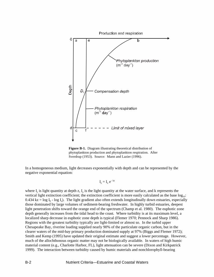
Nutrient Criteria—Estuarine and Coastal WatersB-2
Figure B-1. Diagram illustrating theoretical distribution ofphytoplankton production and phytoplankton respiration. AfterSverdrup (1953). Source: Mann and Lazier (1996).
In a homogeneous medium, light decreases exponentially with depth and can be represented by thenegative exponential equation:
Iz = Io e- kz
where Iz is light quantity at depth z, Io is the light quantity at the water surface, and k represents thevertical light extinction coefficient; the extinction coefficient is more easily calculated as the base log10: 0.434 kz = log I0 - log Iz). The light gradient also often extends longitudinally down estuaries, especiallythose dominated by large volumes of sediment-bearing freshwater. In highly turbid estuaries, deepestlight penetration shifts toward the orange end of the spectrum (Champ et al. 1980). The euphotic zonedepth generally increases from the tidal head to the coast. Where turbidity is at its maximum level, alocalized sharp decrease in euphotic zone depth is typical (Flemer 1970; Pennock and Sharp 1986). Regions with the greatest turbidity typically are light-limited or almost so. In the turbid upperChesapeake Bay, riverine loading supplied nearly 90% of the particulate organic carbon, but in theclearer waters of the mid-bay primary production dominated supply at 97% (Biggs and Flemer 1972); Smith and Kemp (1995) have updated their original estimate and suggest a lower percentage. However,much of the allochthonous organic matter may not be biologically available. In waters of high humicmaterial content (e.g., Charlotte Harbor, FL), light attenuation can be severe (Dixon and Kirkpatrick1999). The interaction between turbidity caused by humic materials and nonchlorophyll-bearing

Nutrient Criteria—Estuarine and Coastal Waters B-3
particulates complicates the direct application of the Secchi disc as a measure of nutrient overenrichment. Spectral radiometers can to some extent partition the various components of light extinction and are thepreferred tools. Modern algal pigment diagnostic tools (e.g., HPLC) can compare water qualityresponses to varying nutrient and other pollutant inputs across various coastal system types (Jeffery et al.1997). It is possible that turbidity may mask the impending development of undesirable algae.
The vertical extinction coefficient for estuaries shows wide seasonal variations. Values frequentlyexceed 0.1 m-1). The extinction in open-ocean waters is often estimated by the relation E.C. = 1.7/Secchi depth in meters. Holmes (1970) and Keefe et al. (1976) both arrived independently at a constantof approximately 1.46 instead of 1.7 for turbid estuarine and nearshore coastal waters. Walker (1980)suggested that the original Poole and Adkins (1929) Secchi disc constant on average gives resultsapproximately 17% too high and suggested a value of 1.45. These corrections should be made and, moreimportantly, it is useful for the constant to be checked for each estuary. For more quantitative work, aquantum light meter that measures over a spectral range of 400-700 nM is preferred. Commercialproducts (e.g., www.licor.com) are now available that can measure the spectral photon flux over a rangeof interest to aquatic scientists.
The extinction coefficient can be broken down into several components. The total light attentuation, KT
= Kw + Kc + Kd + Kp (Lorenzen 1972; Kirk 1983; Bledsoe and Phlips 2000; Koenings and Edmondson1991) can be resolved for the effects of water, chlorophyll a, dissolved substances, and nonalgalparticulate matter. In many estuaries, Kd may contribute between 5% and 50% of the KT. The Kwusually can be ignored because it is such a minor component. In blackwater estuaries receiving highloads of humic materials the Kd may dominant KT. In systems such as the “turbidity maximum zone” inupper Chesapeake Bay, Kp may be the dominant component. The EPA Chesapeake Bay Program hassponsored research to calibrate KT components applicable to SAV beds (www.chesapeakebay.net; searchthe publications database for “Chesapeake Bay Submerged Aquatic Water Quality and Habitat-BasedRequirements and Restorations Goals: A Second Technical Synthesis.”
Among some coastal ecosystems, light (i.e., mean photic depth) and nutrient loading appear to be equallygood predictors of phytoplankton primary production (see Figure 1b in Cloern 1999). This observationstrengthens the proposition that phytoplankton production in these systems can be limited by otherresources and processes in addition to nutrient loading. Pennock and Sharp (1994) suggest that theDelaware River Estuary functions analogously as a chemostat during the summer. They point out thathigh N supplies from upstream advect continually through the brackish-water region into the lowerestuary, where high primary production occurs from remineralized N and the advected supply and thephytoplankton biomass is limited by grazing. Their conclusion is especially significant because evidencealso suggests that bioassay experiments that isolate the water may lead to misidentification of nutrientlimitation. The flushing component in the bay provides the physical analogue to a chemostat, where thenutrient supply and adequate light support high phytoplankton biomass production and grazing andflushing maintain a potentially steady-state phytoplankton biomass, with fluctuations due primarily tophysical forcing factors.

Nutrient Criteria—Estuarine and Coastal Waters C-1
APPENDIX CADDITIONAL INFORMATION ON FLUSHING IN ESTUARIES
by Edward H. Dettmann, U.S. EPA, Office of Research and Development, National Health and Environmental Effects Research Laboratory, Atlantic Ecology Division
A variety of terms such as residence time, flushing time, transit time, turnover time, and age are used todescribe time scales for transport and removal of materials that enter waterbodies. Use of these terms inthe literature is often inconsistent and sometimes imprecise, so that care must be exercised to determinethe meaning of terms being used, to avoid misinterpretation or incorrect comparisons of data. Thisappendix contains definitions of terms and discussions of factors that affect flushing and empirical andmodeling methods for estimating residence times in estuaries. An understanding of residence times isespecially important when estimating not only system responses to nutrients, but also the lag phasebetween management and system improvements.
Definitions of Residence TimesThe freshwater residence time (Jfw) is the average amount of time that freshwater, or a conservative tracerintroduced with freshwater inputs, resides in the estuary before exiting. It is the mean transit time for amolecule of water or conservative tracer to progress from the point of input to the seaward boundary.This is the definition of residence time most often given in the literature, and is generally the most usefulfor analysis of eutrophication in estuaries, as most nutrients are usually introduced with freshwater.
Another commonly used concept is that of the mean amount of time required for water (or ahomogeneously-distributed conservative tracer) that is in the estuary at a given time (regardless ofsource) to leave the estuary. This is here called “estuary residence time”(Je), although Takeoka (1984)and Zimmerman (1976) use the term “residence time.”
The values of Jfw and Je may differ. Consider the case of an elongated unstratified estuary, with theseaward boundary at one end and a river as the single source of freshwater located at the opposite end. Inthis case, the travel distance from the river mouth to the seaward boundary is longer than the averagetravel distance from other parts of the estuary, so that Jfw > Je. Conversely, if the river enters the estuarynear the seaward boundary, Je may exceed Jfw. For cases intermediate between these two, the differencebetween these two residence times becomes smaller, and the times may be equal. Multiple freshwaterinputs and other factors such as stratification and estuary shape may complicate matters, but the sameprinciples apply.
These concepts, the related concepts of turnover time and age, and the relationships among thesemeasures are discussed in detail by Bolin and Rodhe (1973) and Zimmerman (1976), and summarized byTakeoka (1984). Miller and McPherson (1991) discuss another concept, “pulse residence time,” for wateror a conservative constituent introduced as a pulse, that may be useful in some circumstances.
Factors That Influence Residence TimeWater residence times in estuaries are influenced by any factor that affects water movement, includingfreshwater inflow rates, tides, wind, mixing, stratification, and system topography. Because many ofthese factors are variable, residence times are also not static. This variability requires attention to theappropriate time interval over which the residence time should be expressed, and the representativenessof the conditions under which a given measurement is made. A long-term (seasonal or annual) averageresidence time is often most appropriate for analysis of the effects of nutrients.

Nutrient Criteria—Estuarine and Coastal WatersC-2
Freshwater ForcingResidence time may be quite sensitive to freshwater inflow rate, with larger flow rates associated withsmaller residence times. This is illustrated by three Rhode Island estuaries. For Narragansett Bay, Jfw
varies between approximately 10 and 40 days; Jfw at the long-term mean freshwater inflow rate is 26 days(Pilson 1985). For the Seekonk River, Jfw varies between 0.4 and 2.9 days, with a value of 1.2 days forthe mean freshwater inflow rate, and for the Providence River, Jfw varies between 0.7 and 6.3 days, and is2.5 days at average inflow (Asselin and Spaulding 1993).
Tidal ForcingTides can be a major factor controlling estuary-ocean exchange of water and therefore water residencetime. Important factors are the tidal range, tidal frequency (diurnal vs. semidiurnal), and estuary depth.Tidal ranges in U.S. coastal waters range from centimeters to more than 5.5 m. For a given estuary,residence times may vary over the spring-neap tide cycle.
Wind ForcingWind may substantially influence estuarine circulation, and therefore water residence time. In a study oftwo small shallow estuaries, Geyer (1997) found that wind direction (offshore vs. onshore) had asubstantial effect on salinity structure and nontidal flow in one estuary, and Jfw varied by a factor ofapproximately 3 (from 0.8 to 2.7 days) in response to the sea-breeze cycle. Measurements in a nearbyand similarly oriented estuary during the same time period found that whereas wind direction influencedsalinity distributions, a constriction at the estuary mouth limited estuary-offshore exchange, so that therewas no significant relationship between residence time and wind stress. Estuaries bordering the Gulf ofMexico are shallow, highly susceptible to wind forcing, and considered meteorologically dominated(Solis and Powell 1999; Ward 1980).
Determination of Residence TimeA number of empirical and computational methods are used to measure or estimate water residencetimes.
Empirical MeasurementsEmpirical measurements of water residence time depend on measurement of the distribution or dynamicsof tracers (generally freshwater or introduced dye) in estuaries.
Bolin and Rodhe (1973) show that the transit time of a tracer through a reservoir is given by the turnovertime (Jo) , i.e.
where Mo is the total mass of a constituent in the reservoir and Fo is the total flux through the reservoir. This is the basis for the freshwater replacement method for calculating the mean freshwaterresidence time in an estuary. The Jfw is calculated as
where Vfw is the volume of freshwater in the estuary and Qfw is the input rate of freshwater. This ratiogives the time required for the inflowing freshwater to replace the freshwater already in the estuary. Thevolume of freshwater in the estuary is calculated as the amount of freshwater that must be mixed with

Nutrient Criteria—Estuarine and Coastal Waters C-3
seawater having salinity (Ss) equal to that entering at the seaward boundary to yield a volume Ve equal tothat of the estuary, with salinity equal to the mean salinity of the estuary (Se). Vfw may be calculated as
Examples of this method are given by Pilson (1985), Geyer (1997), and Solis and Powell (1999).
Fluorescent dye (usually Rhodamine WT) is also used to determine water residence times. To measurefreshwater residence time, dye is introduced continuously into the inflowing freshwater at a rateproportional to the freshwater flow rate. Dye concentrations are surveyed at (high or low) slack tide. Dye input is terminated when the mean concentration of dye in the estuary reaches equilibrium(approximately 3 times the freshwater residence time). Further periodic surveys are conducted at thesame tide phase to monitor the dye content of the estuary. The average concentration of dye is usuallyfound to follow a decreasing exponential with time,
where Co is the initial average concentration of dye in the estuary and C(t) is the concentration at time t. This function is fit to the data, and the mean residence time of dye in the reservoir, a surrogate for themean freshwater residence time, is then Jfw = 1/k. Alternatively, as the concentration one residence timeafter termination of dye input is C = Co e
-1, the time required to attain this concentration is sometimestaken as the residence time. The estuary residence time may be measured similarly. In this case, the dyeis distributed as uniformly as possible throughout the estuary in a rapid application, and the change indye content is monitored as above. The residence time determined from the rate of change of tracerconcentration is sometimes called the e-folding time. Because of cost and logistical considerations, dyestudies are most often done on relatively small estuaries. Examples of such studies are described by Callaway (1981), Dettmann et al. (1989), and Geyer et al. (1997).
ModelsA wide range of models, ranging from simple to complex, has been used to calculate water residencetime in estuaries. The simplest of these is the tidal prism model, which estimates residence time (innumber of tidal cycles) as the ratio V/P, where V is the estuary volume (usually expressed at high tide)and P is the volume of the tidal prism. The model is based on the assumption that water entering theestuary on the flood tide is thoroughly mixed throughout the estuary within a tidal cycle. Most estuariesdo not meet this requirement and, for all but very small estuaries, this model generally underestimatesestuary and freshwater residence time, sometimes by manyfold.
Ketchum (1951) modified this simple model by dividing the estuary into segments, each having a lengththat corresponds to the local tidal excursion. Water exchanges between adjacent segments during eachtidal cycle are calculated, and complete mixing is assumed to occur only within each segment. Thesegmented tidal prism model requires data for freshwater inputs, tidal range, and estuary topography. Thesimple and segmented versions of the tidal prism model are reviewed by Pritchard (1952) and Dyer(1973), and modified by Dyer and Taylor (1973). For most (but not all) estuaries to which the segmentedmodel has been applied, it has given good results (Dyer 1973). Beyond permitting calculation ofresidence time, segmented tidal prism models permit calculation of the distributions of fresh- and
Nutrient Criteria—Estuarine and Coastal WatersC-4
saltwater and other water quality constituents along the estuary, but do not address the effects of wind onflushing.
Another approach to calculating residence times is the box model. Box models also segment the estuary,assume complete mixing within segments, and calculate diffusive and advective exchanges betweenadjacent segments. These models require data for estuary topography and for freshwater inflows andsalinity distribution in the estuary for each set of conditions to which the model is applied. As actualsalinity data are used, the effects of wind and tide are implicitly taken into account. Applications of suchmodels are described by Brown and Arellano (1980), Dettmann et al. (1992), Hagy et al. (2000), andMiller and McPherson (1991). Such models also allow calculation of advective and diffusive exchangesamong segments and spatial distribution of water quality constituents.
Numerical computer models of hydrodynamics and constituent transport are still more complex. Thesemodels are used to simulate movement of water and water quality constituents at fine spatial resolution,and may also be used to calculate freshwater or estuary residence times. These models generally allowconsideration of wind stress as well as tidal and freshwater forcing. A few examples of such models aredescribed by Brooks et al. (1999), Signell (1992), and Signell and Butman (1992).

Nutrient Criteria—Estuarine and Coastal Waters D-1
APPENDIX D NOAA SCHEME FOR DETERMINING ESTUARINE SUSCEPTIBILITY
(SOURCE: BRICKER ET AL. 1999)
The following provides an overview of the NOAA scheme for determining the overall human potentialfor causing nutrient enrichment of estuaries.
Dilution and Flushing PotentialThe length of time that nutrients spend in an estuary potentially affects their opportunity to contribute tooverenrichment. The time is a function of dilution potential and flushing rate. The analysis usesphysical and hydrologic data to define separately (1) a dilution rating and (2) a flushing rating. In bothcases, the higher rating, the greater the capacity to dilute or flush nutrient loads (see Tables D-1 and D-2).
Figure D-1 combines dilution potential and flushing potential. By combining dilution and flushingcomponents, an export potential (EXP) is determined. Estuaries in the upper left portion of the matrixgenerally have a high EXP that suggests an ability to dilute and flush nutrient loads. Estuaries in thelower right portion of the matrix have the opposite capacity, making them more susceptible to nutrientinput.
Nutrient InputsNOAA used the USGS Sparrow Model (spatially referenced regressions of contaminant transport onwatershed attributes) and other information to estimate nutrient loads and measure nitrogen pressure onestuaries.
Determination of Overall Human-based Nutrient PressureA matrix was used to compare the susceptibility to nutrient retention and the level of N inputs to rank theoverall expression of human influence on eutrophic conditions in the estuary (Figure D-1). Experts at theNational Assessment Workshop reviewed and, where appropriate, modified the assessments based onhigher quality data available for some estuaries; expert knowledge also played a role.

Nutrient Criteria—Estuarine and Coastal WatersD-2
Table D-1. Decision rules for dilution potential
Type IF: vertical stratification THEN: dilution volume IF: dilution value Dilution potential No. estuaries
A Vertically homogenous•all year•throughout estuary
1/VOLestuary 10!13
10!12High 30
B Minor vertical stratification•navigation channels•upper estuary
1/VOLestuary 10!11 Moderate 63
C Vertically stratified•most of year•most of estuary
1/VOLfwf
(fwf=freshwater fraction)10!10
10!09Low 45
Note: This analysis assumes that a larger portion of the water column is potentially available to dilute nutrient loads in avertically homogeneous estuary than in a vertically stratified system. The assumption is that for stratified systems, nutrients aremost often retained in the upper portion (freshwater fraction) of the water column. In contrast, downward transport (morecomplete mixing) is likely in vertically homogeneous systems. Type B estuaries are generally vertically homogeneous, althoughstratification is observed (confined) in narrow navigation channels or the extreme upper reaches of an estuary. In this case,nutrients are assumed to be diluted throughout the entire water column.
Source: Bricker et al. 1999.
Table D-2. Decision rules for flushing potential
Type Tide range (ft) Freshwater inflow/estuary volume Flushing potential No. estuaries
1 Macro (>6) and Large or moderate (1000 to 10!02) High 12
2 Macro (>6) and Small (10!03, 10!04) Moderate 21
3 Meso (>2.5) and Large (1000, 10!01) High 15
4 Meso (>2.5) and Moderate (10!02) Moderate 16
5 Meso (>2.5) and Small (10!03, 10!04) Low 26
6 Micro (<2.5) and Large (1000, 10!01) High 4
7 Micro (<2.5) and Moderate (10!02) Moderate 13
8 Micro (<2.5) and Small (10!03, 10!04) Low 31
Note: This analysis assumes that a greater capacity to flush nutrient loads exists for estuaries that have large tide and freshwaterinfluences.
Source: Bricker et al. 1999.

Nutrient Criteria—Estuarine and Coastal Waters D-3
Figure D-1. Estuarine Export Potential Susceptibility.

Nutrient Criteria—Estuarine and Coastal Waters E-1
APPENDIX ECOMPARATIVE SYSTEMS EMPIRICAL MODELING APPROACH:
THE EMPIRICAL REGRESSION METHOD TO DETERMINE NUTRIENT LOAD-ECOLOGICAL RESPONSE RELATIONSHIPS FOR
ESTUARINE AND COASTAL WATERS
By James Lattimer, USEPA, Office of Research and Development, National Health and Environmental Effects Research Laboratory, Atlantic Ecology Division
The empirical regression method can be used to determine the response of estuarine systems to nutrientloading. This method can take two forms: single system and comparative-systems approaches.
In single system approaches, ecological responses and nutrient concentrations are measured over time ina single system. This allows for the development of load-response models for the individual systems thatare robust because many of the controlling factors, such as, for example, physiographic setting, primaryproductivity base, and hypsography, are relatively constant. This approach has been used to developmodels of the response of primary productivity to nitrogen load (Figures E-1a,b) (Boynton et al. 1995).However, this approach is only applicable to the system in which it was developed and thus is notconsidered to be very useful in the development of widely applicable nutrient load-responserelationships. Single system empirical studies, however, may be useful in providing data on processesuseful for numerical model development.
The alternative approach, using the space for time paradigm (Picket,1988), posits that relationshipsbetween nutrient inputs and ecologically meaningful estuarine responses, using multiple systems, havepredictive capability, at least for the category of systems used in the model development. This allows fora wide range in nutrient loading and estuarine types to be included. The comparative-systems empiricalapproach has been used to determine, for example, relationships between nutrient inputs and fish yields(Lee and Jones 1981; Nixon 1992), benthic biomass, production and abundances (Josefson andRasmussen 2000), summer ammonia flux (Boynton et al., 1995), chlorophyll-a concentration (Boynton etal. 1996; Boynton and Kemp 2000; Monbet 1992), primary productivity (Nixon et al., 1996), and thedominant source of primary productivity (Nixon et al. in press). In many of these cases, importantenvironmental factors such as flushing time and depth, are used to normalize the nutrient loading in asimilar way as Vollenweider (Vollenweider 1976) to yield more precise relationships.
The comparative-systems empirical approach has been successfully used in a regulatory framework todevelop total maximum loads for 30 subestuaries within Buzzards Bay in Massachusetts (Costa et al.1999). Using a citizens’ monitoring network, many important water quality variables were measuredduring summer sampling periods over a five to seven year period. Nitrogen inputs were estimated from aland-use model modified from Valiela (Valiela et al., 1997) augmented with literature data on pointsource and atmospheric inputs. In this study, nitrogen load-response relationships were derived fornitrogen concentration, chlorophyll-a, secchi depth, dissolved oxygen concentration, and eelgrass habitatratio. Nitrogen loadings were normalized to account for volume and flushing time of each of the systemsto improve the precision of the empirical models. An example of the types of relationships determinedusing this approach are given in Figure E-2. The regional estuarine management program used thismethod to adopt total maximum annual loads (TMALs) for nitrogen. Specifically, “...the nitrogenmanagement strategy represents a linking of estimates of watershed nitrogen loading...to empiricalobservations of ecosystem response in a wide variety of Buzzards Bay embayments” (Costa 2000).
The comparative-systems empirical approach does not explicitly consider the processes that produce theobserved phenomena; however, factors known to affect behavior are determined in order to reduce the

Nutrient Criteria—Estuarine and Coastal WatersE-2
Figure E-1a. Scatter plots showing correlation between nitrogen loading, expressedusing the volume Vollenweider-term flushing scale, and 92-98 mean +/- std. errors of theAlternate Eutrophication Index scoring (without oxygen scores).
uncertainty in the models. The smaller the variance in the load-response relationship, the morecompelling the association. One important question for management is to determine what level ofvariance is sufficient to convince stakeholders to accept nutrient limits and associated monetaryexpenditures.
This approach is largely based on statistical associations and is therefore restricted to prediction withinthe class of systems used in the model development. Applicability improves, however, by the inclusionof systems that encompass a wide range in loading and responses. The comparative-systems empiricalapproach allows for the direct measurement of important endpoints (e.g., hypoxia, SAV loss, biomass)obtained in the environment. The endpoints are what are important to the general public. So byproviding a mathematical relationships between the stressor and important endpoints, managers canconvince the public of the importance of regulatory action.

Nutrient Criteria—Estuarine and Coastal Waters E-3
Figure E-1b. Ratio of eelgrass habitat area to potential habitat area versus nitrogenloading, expressed using the volume Vollenweider-term flushing scale (from Costa et al.,1999).

Nutrient Criteria—Estuarine and Coastal WatersE-4
Figure E-2. Plot of annual TN loading rates versus phytoplankton primary production rates at asingle station in the Chesapeake Bay from 1971-76 and 1985-90. Source: Boynton et al., 1995.
Nutrient Criteria—Estuarine and Coastal Waters F-1
APPENDIX FSELECTED THEORETICAL APPROACHES TO CLASSIFICATION OF
ESTUARIES AND COASTAL WATERS
Several theoretical schemes have been presented that may facilitate classification of estuaries and coastalwaters if the need arises for more theoretical approaches. In most cases, these schemes have potentialfuture value but are not likely to be immediately useful. The information-thermodynamic approachoffered by Ulanowicz would seem to provide useful insights to development of an eutrophication indexand may be worth an earlier consideration.
Functional AttributesOdum and Copeland (1974) proposed a classification scheme based on the idea that an ecosystem is abalance between energies that build structure and order, or ordering energies, and energies that causeloss of structure and order, or disordering energies. Although this approach is of theoretical interest, thedata to apply it are still largely unavailable. There are conceptual difficulties. Energy sources andstresses are not always mutually exclusive categories. Day et al. (1989) give several examples of caseswhere moving water can be either an energy source or a stress, depending on the situation. Moderatecurrents are a source of energy for seagrass meadows, because they transport organic matter andinorganic nutrients to beds and remove metabolic wastes. If currents are too strong, however, they candisrupt beds and act as disordering energies.
Theoretic IndicesThis approach is data intensive and has potential as appropriate estuary data are generated. Ulanowicz(1986, 1997) described an approach based on flow analysis and information theory. The idea is that anecosystem can be characterized in terms of growth and organization. Growth is defined as an increase insystem activity or total system throughput (analogous to total system energy flow). Organization isequated with the mutual information inherent in the trophic flow structure. To apply this approach, onewould need to obtain energy flow values (or organic carbon-based equivalents) among trophiccompartments. Following Ulanowicz’s formulation, one could develop an information index ofeutrophication. Compiling such would entail an assessment of the growth and organization status of aeutrophic or nutrient-enriched system compared with a current reference system, a minimally impairedsystem, or an estimate of pre-eutrophication values from historical data. The ratio of growth andorganization of a nutrient-enriched system to its reference value would express the degree of impairment. Such information could help guide restoration priorities. The downside is that the approach requires theavailability of a rich ecological database.

Nutrient Criteria—Estuarine and Coastal Waters G-1
APPENDIX G
EXAMPLES OF NUTRIENT CONCENTRATION RANGES AND RELATEDHYDROGRAPHIC DATA FOR SELECTED ESTUARIES AND COASTAL WATERS IN
THE CONTIGUOUS STATES OF THE UNITED STATES
Atlantic Coast Systems
BOSTON HARBOR, MA (Source: Kelly 1998)WAQUOIT BAY, MA (Source: Valiela et al. 1992) SEEKONK-PROVIDENCE RIVER REGION OF NARRAGANSETT BAY, RI (Source: Doering et al. 1990)WESTERN LONG ISLAND SOUND AND HUDSON-RARITAN ESTUARY, NY/NJ (Source: O’Shea and Brosnan 2000)HUDSON RIVER, NY (Source: Lampman et al. 1999)DELAWARE RIVER ESTUARY (Source: Lebo and Sharp 1993)MARYLAND COASTAL BAYS (Source: Boynton et al. 1996)CHESAPEAKE BAY, MD/VA (Source: Magnien et al. 1992) CHESAPEAKE BAY (Harding and Perry 1997)YORK RIVER ESTUARY, CHESAPEAKE BAY, VA (Source: Sin et al. 1999)NEUSE RIVER ESTUARY, NC (Source: Rudek et al. 1991)CAPE FEAR RIVER ESTUARY, NC (Source: Mallin et al. 1999)COASTAL GEORGIA (Source: Hopkinson and Wetzel 1982)
Gulf of Mexico Estuaries
GULF OF MEXICO CASE STUDIES (Source: Bianchi et al. 1999)GALVESTON BAY, TX (Source: Santschi 1995)
Pacific Coast Systems
EMBAYMENT OF PUGET SOUND, WA (Source: Bernhard and Peele 1997)

Nutrient Criteria—Estuarine and Coastal WatersG-2
The study area (N latitude and W longitude) in Boston Harborand western Massachusetts Bay. The boundary between theHarbor and the Bay is defined by the solid line from DeerIsland to Hull combined with the dashed lines showing the 2high-resolution transects, the spatial limits of data for boxmodeling are depicted. Dots position some watercolumnmonitoring stations that were sampled during 1994. Stationsprefixed with ‘N’ surround the future offshore outfall, which iscentered between Stns N20P and N16P about 15 km fromDeer Island. Data from 2 lines of Bay staions (N01P to N10Pand N04P to N07P, each representing about 10 km distance)were used to provide approximate concentrations for the futuretidal source region for the Harbor.
Boston Harbor

Nutrient Criteria—Estuarine and Coastal Waters G-3
Bay (C0) and Harbor (C1) concentration data used in calculating Harbor-Bay exchange. BA: beam attenuation fromtransmissometer readings; nd: not determined.

Nutrient Criteria—Estuarine and Coastal WatersG-4
Time course of light, temperature,oxygen, ammonium, phosphate, andchlorophyll in water of Waquoit Bay,summer 1988. Modified from Costa et al.(in press).
Waquoit Bay

Nutrient Criteria—Estuarine and Coastal Waters G-5
Vertical profiles of oxygen in Childs River during dawn and midafternoon
of a sunny day (circles), and during afternoon after three cloudy days in a
row. Data from C. D’Avanzo.

Nutrient Criteria—Estuarine and Coastal WatersG-6
Station locations, Solid lines delimit boxes used
in modeling effort. BR=Blackstone River, BV=
Blackstone Valley Sewage Treatment Plant
(STP), TM= Ten Mile River, MR Moshassuck
River, WR=Woonasquatucket River, FP=Field’s
Point STP, EP=East Providence STP, PR=
Pawtuxet River
Seekonk—Providence River Region,Narragansett Bay

Nutrient Criteria—Estuarine and Coastal Waters G-7
Mean and range of salinity and nutrient concentrations observed insurface waters (depth=1.0m) during the six cruises, versus distancefrom the Main Street Bridge, Pawtucket, Rhode Island at the headof the Seekonk River.

Nutrient Criteria—Estuarine and Coastal WatersG-8
Mean and range of salinity and nutrient concentrations observed in bottom
waters (1.0 m from bottom) during the six cruises, versus distance from the
Main Street Bridge, Pawtucket, Rhode Island at the head of the Seekonk
River.

Nutrient Criteria—Estuarine and Coastal Waters G-9
Location of New York City Department of Environment Protection’s Harbor Survey Water Quality
Monitoring Stations. Also depicted are the 14 New York City Water Pollution Control Plants and the 8
New York City sludge dewatering facilities (shaded boxes). Sandy Hook, lower center, is located at
approximately 40°30'N, 74°W.
Western Long Island SoundHudson-Raritan Estuary
LOCATION OF WPCP’s AND SAMPLING STATIONS IN NY HARBOR

Nutrient Criteria—Estuarine and Coastal WatersG-10
Key water quality indicators for summer (June–September) of 1999. Depicted are: bottom minimum
dissolved oxygen (upper left) in mg l!1; summer average dissolved inorganic nitrogen
[NH3!N+(NO3+NO2)!N] (upper right) in mg l!1; summer average Secchi transparency (lower left) in m;
summer average total phosphorus (lower right) in mg l!1.

Nutrient Criteria—Estuarine and Coastal Waters G-11
1989–1999 summertime (June–September) average ambient dissolved inorganic nitrogen [dissolved
ammonium-nitrogen (NH4-N) and dissolved nitrate- and nitrite-nitrogen (NO3)-N] concentrations (mg l!1 for
western Long Island Sound, Raritan Bay, and Jamaica Bay stations. Trends in summertime average
concentrations are noted where significant (p < 0.05).

Nutrient Criteria—Estuarine and Coastal WatersG-12
1989–1999 summertime (June–September) average ambient total phosphorus (TP) and dissolved
orthophoshpate (PO4-P) concentrations (mg l-1) for western Long Island Sound, Raritan Bay, and Jamaica
Bay stations. Trends in summertime average concentrations are noted where significant (p < 0.05).

Nutrient Criteria—Estuarine and Coastal Waters G-13
Map of the tidal freshwater Hudson River, its watershed
and major tributaries. The inset shows the location of the
watershed of the watershed of the Hudson, primarily in
eastern New York State. The main panel shows the
watershed of the Hudson. The upper (non-tidal) tributaries
are in white and their surrounding watershed is shaded.
The remaining, unshaded, section of the watershed
delivers water to the tidal Hudson River (heavy black line)
primarily through 7 tributaries. These tributaries (creeks)
are labeled: K for Kinderhook; Cfor Catskill; RJ for
Roeloff Janson Kill; E for Esopis; R/W for
Rondout/Wallkill; WP for Wappingers; Cr for Croton.
The first 5 of these tributaries enter within the budgeting
reach (labeled) between km 225 and 125. The section of
the river that was sampled during our transect sampling
(labeled sampling stretch) is also shown.
Hudson River, NY

Nutrient Criteria—Estuarine and Coastal WatersG-14
Box and whisker plots for forms of N and P for the
entire data set of the Hudson. The data include all
samples taken from January 1992 to December 1996
and combine seasonal and spatial variation. Shown are
the medians, upper and lower quartiles and 90%
inclusion lines. The number of samples for each
analysis is labeled near the boxes.

Nutrient Criteria—Estuarine and Coastal Waters G-15
Spatial variation in selected variables for a
representative transect taken in early September
1996. Transects run km 240 (Albany
downstream to km 40. For each variable
samples were taken every 2 to 4 km. Units are,
conductivity—(note log scale); pH—normal pH
units; chlorophyll a— 1-1; turbidity— NTU; N
and P—µM. For both N and P the per line
represents total N and toal P. “Other N” is TN
minus DIN (NH4 plus NO3); For P, “Other P” is
TP minus phosphate.

Nutrient Criteria—Estuarine and Coastal WatersG-16
The Delaware Estuary with insert showing relation to
the mid-Atlantic coast of the United States. Stations
(1-9, 11-26) were located along the main axis of the
estuary, every 5-15 km. Station 10 was located in the
Schuylkill River (not shown). The river is tidal from
the mouth of the bay up to the fall line at Trenton,
New Jersey (240 km). Salinity increases from 0.1%
at station 14 (130 km) to 30% at the bay mouth. The
majority of TP inputs to the river are clustered
between stations 6-9.
Delaware River Estuary

Nutrient Criteria—Estuarine and Coastal Waters G-17
Figure 16Average biological, chemical, and physical parameters for Delaware Estuary 1986-1988. Values
are the nonweighted mean of 17 to 24 discrete samples taken at each location (Lebo et al. 1990). Data are
shown for locations near the Delaware River (station 2), Philadelphia (station 7), beginning of the salinity
gradient (station 14), turbidity maximum (station 16), downstream of the turbidity maximum (station 20), and
in the lower bay (station 23). In addition, average relative standard deviation (RSD) for all stations is shown.
The average standard deviation for station location and salinity was 1.1 km and 2.1%, respectively.

Nutrient Criteria—Estuarine and Coastal WatersG-18
Map of the Maryland coastal bays complex indicating the boundaries of the watershed and a
subsystems for which nitrogen inputs were estimated.
Maryland Coastal Bays

Nutrient Criteria—Estuarine and Coastal Waters G-19
Summer average chlorophyll a concentrations for representative regions of the Maryland coastal bays
based on samples collected during 1975, 1983, and 1991. Data are from Fang et al. (1977a,b), Maryland
Department of Health and Mental Hygiene (1985), and National Park Service (1991).

Nutrient Criteria—Estuarine and Coastal WatersG-20
Map of Chesapeake Bay region showing tributaries, sampling sites, and major wastewater
treatment plants for systems examined or referenced in this paper. The major wastewater
treatment plants are as follows: 1) Western Branch, 2) Arlington, 3) Blue Plains, 4)
Alexandria, 5) Piscataway, 6) Little Hunting Creek, and 7) Lower Potomac.
Chesapeake BayMagnien et al.

Nutrient Criteria—Estuarine and Coastal Waters G-21
Salinity dilution plots of nitrate plus nitrite,
ammonium, total nitrogen, orthophosphate, and total
phosphorus for surface samples at all Chesapeake
Bay Mainstream stations. Each point represents a
single station at which median values were calculated
for each seasonal time frame (see Fig. 2) over the
entire 195-1989 period. All stations identified in Fig.
1 were plotted in longitudinal order starting at the
head of the estuary. The circled point for each
seasonal plot is the upper mesohaline plankton station
at the Annapolis Bay Bridge.

Nutrient Criteria—Estuarine and Coastal WatersG-22
Concentrations of ammonium (µM) in Back River, and ammonium concentrations, primary productionestimates (mg C m-2 d-1) and temperature (BBC) for the Patapsco River(Baltimore Harbor). Values presentedare surface mixed layer medians by month from continuous monitoring at a frequency of one to two times permonth over the period 1985-1989. Station locations are centrally located in each system (see Fig. 1)
Month
Back River Patapsco River
NH4+ NH4
+ Primary Production Temperature
January 257.0 8.9 299 3.2
February 414.0 48.2 1,384 3.0
March 112.4 24.3 640 6.2
April 439.0 33.6 663 12.3
May 151.7 11.7 1,520 16.8
June 35.7 9.7 1,840 24.3
July 82.1 13.0 2,263 27.2
August 87.5 30.3 1,950 26.6
September 107.1 18.8 1,744 23.8
October 103.5 21.3 953 17.7
November 232.0 15.4 751 11.3
December 317.7 13.1 930 6.5
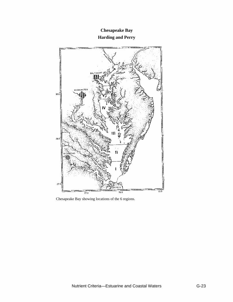
Nutrient Criteria—Estuarine and Coastal Waters G-23
Chesapeake Bay showing locations of the 6 regions.
Chesapeake Bay
Harding and Perry
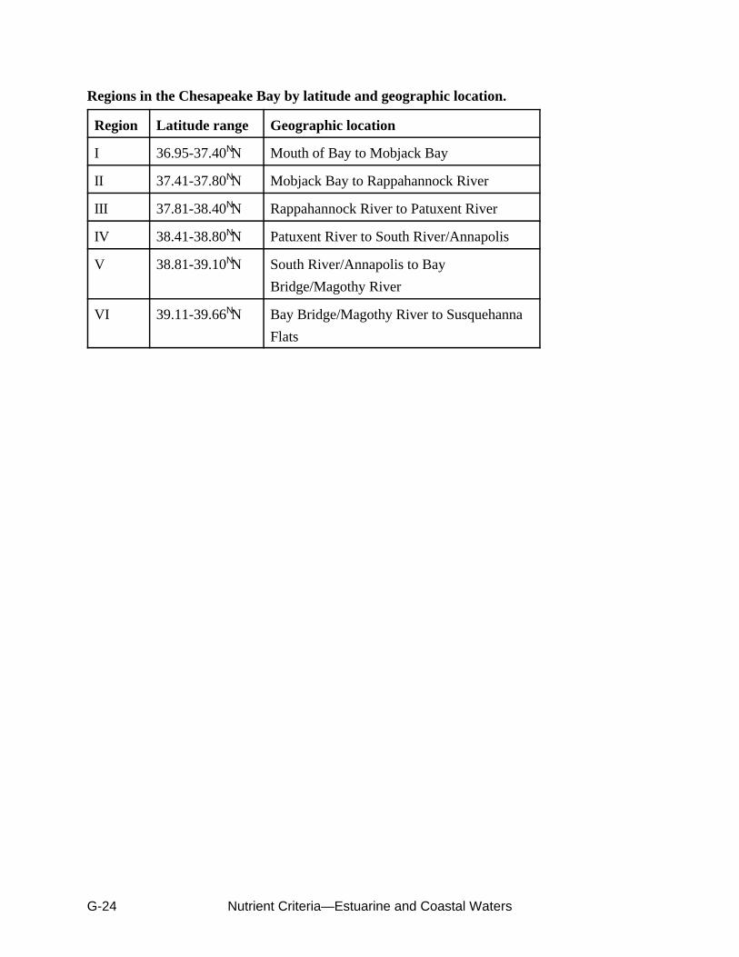
Nutrient Criteria—Estuarine and Coastal WatersG-24
Regions in the Chesapeake Bay by latitude and geographic location.
Region Latitude range Geographic location
I 36.95-37.40NN Mouth of Bay to Mobjack Bay
II 37.41-37.80NN Mobjack Bay to Rappahannock River
III 37.81-38.40NN Rappahannock River to Patuxent River
IV 38.41-38.80NN Patuxent River to South River/Annapolis
V 38.81-39.10NN South River/Annapolis to Bay
Bridge/Magothy River
VI 39.11-39.66NN Bay Bridge/Magothy River to Susquehanna
Flats

Nutrient Criteria—Estuarine and Coastal Waters G-25
Summary statistics on surface chlorophyllconcentrations (mg m-3) from Monitoring Programcruises on the Chesapeake Bay, 1985-1990.

Nutrient Criteria—Estuarine and Coastal WatersG-26
The Environmental Protection Agency Chesapeake Bay Monitoring stations in theYork River estuary.
York River

Nutrient Criteria—Estuarine and Coastal Waters G-27
Seasonal distributions of chlorophyll a and primary production in the York River system;monthly means and standard errors were calculated from the 10 years data (1985-1994)for chlorophyll a and from 7 years data (1988-1994) for primary production. Dashed lineat 10 µg 11-1 indicates our criterion for algal blooms and primary production shown in Fig3F was measured at WE4.2.

Nutrient Criteria—Estuarine and Coastal WatersG-28
Salinity dilution curves of DO, ammonium, orthophosphate, silicate, nitrite + nitrate,chlorophyll a and light attenuation coefficient in the water column of the York River systemfor low (1991), mean (1990) and high (1994)flow years during the summer-fall period (Junethrough October).

Nutrient Criteria—Estuarine and Coastal Waters G-29
Sampling locations (Stns 1, 5, and 6) in the lower Neuse River Estuary,North Carolina, USA.
Neuse River Estuary, NC

Nutrient Criteria—Estuarine and Coastal WatersG-30
Neuse River mean monthly flows (× 1000 ft3 s-1 or × 28.3m-3 s-1), at the US Geological Survey gauging station inKinston North Carolina. Dashed line represents 60 yraverage flow (J.D. Bales, US Dept of Interior, GeologicalSurvey, Water Resources Division, Raleigh, NorthCarolina). (Middle) Surface measurements of salinity atStns 1, 5, and 6 (see Fig. 1). Continuous line representsmeans of stations measure. (Bottom) Monthly rainfalltotals at the Institute of Marine Sciences, Morehead City,North Carolina. Dashed line represents average monthlyprecipitation for the southern section of the Albermarle-Pamilico estuarine system area (118.5 mm mo-1) (H.Porter, University of North Carolina Institute of MarineSciences, Morehead City).

Nutrient Criteria—Estuarine and Coastal Waters G-31
Nitrate, ammonium, and phosphate concentrations insurface waters at Stns 1, 5, and 6 (see Fig. 1). Continuous line represents means among stations.

Nutrient Criteria—Estuarine and Coastal WatersG-32
(Top and middle) Chlorophyll a concentration of selectednutrient addition treatments minus controls, averaged overthe 4 d of each bioassay. N(14.3) and N(28.6) respectivelyindicate addition of 14.3 and 28.6 µm NO3- P(3.2) indicatesaddition of 3.2 µm PO4
3-. Error bars not visible are smallerthan symbol. (Bottom) Dissolved inorganic nitrogen:dissolved inorganic phophorus (DIN:DIP) ratio (by atoms). No error bars plotted.

Nutrient Criteria—Estuarine and Coastal Waters G-33
(Top and middle) 14C assimilation of selectednutrient addition treatments minus xontrols,averaged over the 4 d of each bioassay. Symbolsas in Fig. 4 (Bottom Nitrate, ammonium, andphosphate concentrations in surface waters at Stn 6(see Fig. 1). Data are compiled from Fig.3 andpresented here for comparative puposes.

Nutrient Criteria—Estuarine and Coastal WatersG-34
Sampling stations along the Cape Fear River Estuary, North Carolina,
United States. The lower estuary is centered in 33°56NN, 77°58NW.
Cape Fear River Estuary

Nutrient Criteria—Estuarine and Coastal Waters G-35
Physical parameters for selected stations in the Caper Fear River
Estuary, June 1995-November 1998.

Nutrient Criteria—Estuarine and Coastal WatersG-36
Inorganic nutrient concentrations for selected stations in the Cape
Fear River Estuary, June1995- November 1998.

Nutrient Criteria—Estuarine and Coastal Waters G-37
Coastal Georgia
Nutrient exchange (::g-atom m-2 d-1) across the sediment/water interface and initial nutrientconcentrations (::g-atom 1-1) in the overlying water of the nearshore environment. Valuesgiven as release (+) or uptake (-) of the nutrient by the sediment.
Constituent Initial Concentration ::M
O2 6.5
NH4+ 1.1
NO2- 0.11
NO3- 0.16
DON 24.3
PO4/ 1.4
DOP 0.0
E Inorganic nitrogen 1.26
E N 25.56
E Inorganic phosphorus 1.4
E P 1.4

Nutrient Criteria—Estuarine and Coastal WatersG-38
Map showing the distribution of estuaries in the Gulf of Mexico.
Gulf of Mexico Estuaries

Nutrient Criteria—Estuarine and Coastal Waters G-39
SiteArea(km2)
Volume (106 m3)
MeanDepth
(m)
MaximumLength
(km)
MaximumWidth(km)
Florida Bay, FL 1800 3200 2.0 70.0 40.0 Carbonate system lowfreshwater input
Tampa Bay, FL 896 3490 3.9 61.1 16.1 Marine dominated estuary
Apalachicola Bay, FL 593 1600 2.7 12.9 33.8 River dominated with micro-tides
Mobile Bay, AL 1060 3200 3.0 48.5 40.0 River dominated withseasonal coastal plume
Fourleague Bay, LA 56 72.8 1.3 16.0 3.5 Shallow, wetland dominatedsalinity variable usually low.
Nueces River Estuary,TX
538 1290 2.4 28.2 12.9 Event driven estuary, lowriver flows
Celestun Lagoon,Mexico
28 33 1.2 20.7 2.1
Freshwater spring-fedlagoons.
Chelum Laggon,Mexico
13.6 16.3 1.0 14.7 1.8
Dzilam Lagoon,Mexico
9.4 11.2 0.8 12.9 1.6
Rio Lagartos Lagoon,Mexico
96 76.8 0.8 80.0 1.5
Table 5-1. Physical Characteristics of Gulf Estuaries Examined in Case Studies.

Nutrient Criteria—Estuarine and Coastal WatersG-40
Annual Mean and Range of Salinity and Nutrient Concentrations for Gulf Estuaries Examined in the Case Studies.
Annual mean and range of Chlorophyll-a Primary Production of Gulf Estuaries Examined in the Case Studies.

Nutrient Criteria—Estuarine and Coastal Waters G-41
Average Concentrations of Nutrients and Other Chemical Parameters in Galveston Bay, Calculated from theTWC Database (± 1F).
Galveston Bay

Nutrient Criteria—Estuarine and Coastal WatersG-42
Map showing location of Padilla Bay in relation to Puget Sound (left) and the study site (X) inPadilla Bay.
Puget Sound
Padilla Bay

Nutrient Criteria—Estuarine and Coastal Waters G-43
Dissolved inorganic nutrient concentration in surface water at thestudy site from June to October 1992.
DIN:PO43- ratios and chlorophyll a concentrations in surface water at
the study site from June to October 1992. DIN is NO3- + NO2
- + NH4+.
PO43- is soluble reactive phosphate. The dotted line represents the
Redfield ratio of 16:1.

Nutrient Criteria—Estuarine and Coastal Waters H-1
APPENDIX HPRELIMINARY STATEMENT OF PROPOSED NEAR COASTAL MARINE
NUTRIENT SAMPLING AND REFERENCE CONDITIONDEVELOPMENT PROCEDURE
Synopsis of the National Nutrient Criteria Program, Coastal Marine Sampling Design Planning Meeting, 4-5 June 2001, USEPA Environmental Science Center, Ft. Meade, MD.
Near Coastal Marine Nutrient Sampling and Reference Condition Development Committee Members:Barry Burgan, USEPA; John Fox, USEPA; Laura Gabanski, USEPA; Jeroen Gerritsen, Tetra Tech Inc.;George Gibson, USEPA*; William Muir, USEPA; Kent Price, Univ. Del.; Don Pryor, NOAA; GregSmith, GLEC, Inc.; Val Smith, Univ. Kansas; and Jack Word, MEC Analytical Systems, Inc.
*Contact: USEPA Laboratory, 701 Mapes Road, Ft. Meade, Md. 20755-5350. Phone: (410) 305-2618E-mail: [email protected].
Background and PurposeCultural eutrophication is an established water quality management concept and concern reaching as farback as the 1600s in America (Capper, Power and Shivers 1983). However, extensive public recognitionof this form of pollution in coastal waters is relatively recent. The publication “Eutrophication, Causes,Consequences, and Correctives” (NAS 1970) is often perceived as the technological beginning ofAmerican nutrient pollution awareness and is centered on the understanding and abatement of thisproblem primarily in freshwater lakes and reservoirs. We have since come to better understand theproblem in streams, rivers and estuaries with the publicity and public involvement in the Chesapeake Baystudies of the 1980s. Vollenweider, Marchetti, and Viviani published “Marine Coastal Eutrophication”in March of 1992 and this volume may be considered the coastal equivalent of the land mark NASfreshwater publication a decade earlier.
In response to this growing awareness, the EPA National Nutrient Criteria Program is preparing technicalguidance for nutrient reference condition determination and related criteria development to be used byStates and Tribes in the reduction of cultural eutrophication of the Nations’ surface waters. This reportconcentrates on coastal marine waters and the effort to identify relatively natural nutrient water qualityconditions, which can be used as a benchmark to evaluate cultural eutrophication or overenrichment. Apreliminary literature investigation and data search indicate that insufficient data exist to derive thereference condition information suitable for the needs of the Program without going to primary datacollection.
Because data gathering is likely to be a preliminary concern as well as an ongoing requirement, thismeeting of coastal marine nutrient research and management specialists was called to design a standardprotocol that the EPA can recommend for use in U.S. marine coastal waters. Coastal marine waters aredefined as those waters within 20 miles of shore along the East, West, and Gulf coasts of the UnitedStates as well as Alaska, Hawaii, and the U.S. Trust Territories. Emphasis is on the three mile limit Statewaters, although interest may devolve to the 12- mile U.S. limit as well. Nutrient loading from culturalland run off sources are not presently expected to be a serious problem beyond this limit. The generaldesign and protocol are applied here to a case study example, the coastal waters of the mid-Atlantic Bightfrom New Jersey to the Virginia Capes. Many of the design elements, in particular the number, size andplacement of spatial elements (strata and cells; see below) would need to be modified for specificapplications in different parts of the U.S. coastline.

Nutrient Criteria—Estuarine and Coastal WatersH-2
A coastal transect of fixed stations exists for most of the Mid-Atlantic Bight, which has been used byEPA and NOAA for several years to collect nitrogen, phosphorus, Secchi depth (SD), and chlorophyll-a (Chl-a) data. This procedure and data base will be the prototype presented and discussed to develop therecommended protocol.
ObjectiveTo determine a simple, cost effective, scientifically defensible and standardized method to sample formarine enrichment variables to use in determining reference condition for nutrient criteria derivation.
Premise of the National Coastal Nutrient Criteria ProgramOffshore marine and onshore, near-coastal sites removed from point and estuarine discharges can beidentified as reference sites reflecting the least culturally impacted nutrient water quality of a region. “Region” in this case is a geographically similar portion of the coastline such as the Mid-Atlantic Bight. Such regions can also be described from the coastal portion of the Level III nutrient ecoregion map of thecontinental United States (which is consistent with the rest of the National Program and is similar to theORD Provinces used by EMAP).
Nutrient water quality is established from representative sampling of the coastal waters at these a priorireference sites. The other elements of nutrient criteria, i.e., historical trends, modeling of the data foradditional insights, and attention to the consequences down-current of any proposed nutrient criteria, andassessment of all of this information by a Regional Technical Assistance Group (RTAG) are applied tothe initial reference condition values to develop nutrient criteria for total phosphorus (TP), total nitrogen(TN), Chl-a, and SD.
These criteria can then be used by States and Tribes to manage and monitor the nutrient quality of theircoastal marine waters. While this concept was developed and initiated by the USEPA beginning with theBiological Criteria Program in 1989 (EPA-440/5-90-004, EPA-440/5-91-005) and further refined andapplied to nutrients by the EPA National Nutrient Criteria Program in 1995 (EPA 822-R-96-004, EPA822-R-98-002), the idea has also been independently developed by the Swedish EnvironmentalProtection Agency using the reference condition approach on a regional basis and employing the sameindicator variables (Report number 5052, 2000).
ImportanceAll other waters of the continent drain to the coast and these coastal marine areas are the recipient of anynutrients not intercepted from that cumulative runoff. Globally, conditions of many coastal areas haveshown several-fold increased levels of nitrogen and phosphorus since industrialization (Smith 1998,Smith, Tilman and Nekola 1999), and preliminary assessments of empirical data collected from the Mid-Atlantic Bight between New Jersey and North Carolina by USEPA Region III since 1987 have suggestedan upward trend in the concentration of both dissolved inorganic nitrogen (DIN) and dissolved inorganicphosphorus (DIP) at stations approximately 1 to 5 nm off shore (Muir, pers com, 2001). An extensivebaseline of region specific coastal nutrient data, regularly and consistently collected, is needed toestablish criteria against which future loading conditions may be compared. Potential predictive modelsmay also be developed from this information relating algal booms and other biological responses to thesenutrient levels in coastal waters.
The Transect Sampling DesignAs illustrated below (Figure H-1, of coastal sampling stations between Atlantic City, NJ and Kitty Hawk,NC) a series of transect sampling stations have been located between one and five miles from shore alonga designated coast line to measure ambient water quality as reflected in TN, TP, Chl-a and SD. Datacollected from those stations determined to be remote from significant cultural impacts such as sewage

Nutrient Criteria—Estuarine and Coastal Waters H-3
Figure H-1. Example of an initial coastal monitoring project conducted off the mid-Atlanticshelf just north of Delaware Bay and south of the mouth of the Chesapeake Bay toobtain nutrient reference condition values. Open circles are reference sites and theinshore references are compared to the offshore ones for confirmation.

Nutrient Criteria—Estuarine and Coastal WatersH-4
discharges, industrial activities, major port facilities, or estuarine discharges constitute the referencecondition. The values measured can be compared to marine conditions further offshore (e.g., 20-25 nm)reflecting, at least for TN and TP, the unimpacted condition.
This comparison, together with attention to prevailing currents including upwellings, would establish theseasonal values for TN, TP, Chl-a, and SD. Salinity would also be an important variable to documentlocal constancy of the waters and to avoid discharge plumes from rivers and estuaries that are not part ofthe defined coastal waters of concern. These estuarine and riverine waters should have their own criteria.
Data have been collected from the surface 1 meter, mid depth, and the bottom 1 meter of the watercolumn at each station. Measurements are made on a seasonal basis, essentially mid-summer and mid-winter and with sufficient data, criteria can be established for each season. While the protocol asdescribed above has been in use for about twenty years, most of those data are for dissolved inorganicnitrogen and phosphorus rather than TN and TP, Chl-a, and SD. The TN, TP and off shore stations are arecent addition and only two summers of data are available which is reported here.
Data CollectionOperations are during daylight hours only in order to include SD measurements with surface nutrientcollections and to maintain a consistent nutrient depth profile relative to photo periodicity. Additionaldata collected with a CTD includes salinity, pH, temperature, depth, conductivity, and DO.
Data sampling points presently include the discharge plumes of estuaries, rivers, and point dischargers tomonitor impacts and design management plans, but not as part of the proposed coastal referencecondition sampling system per se.
The Pilot ProjectThe area approximately between Atlantic City, NJ and Kitty Hawk, NC has been studied by EPA RegionIII for about 17 years and includes a mix of nutrient, chemical, biological, and physical measurements. This data has been processed and will provide trend information about the area.
For the last two summers and one winter, nutrient data have been collected from this area in the mannerdescribed above. This is the initial basis for a reference condition determination and is presented inFigures H-2 a-d, below.
If the pilot project is judged successful, it is expected that the process, training, and funds for similarequipment will be provided to each of the coastal EPA Regions for comparable operations to developtheir ecoregional coastal nutrient criteria. This area more than any other because of the proximity ofState and Federal waters will lend itself to joint data gathering and criteria development.
Methods and MaterialsForty-nine sampling stations are located along the 200 nautical mile (nm) stretch of coastal waters. There are twenty stations roughly 10 miles apart situated one to five miles off shore (total of 39consisting of either single stations or sets of two or three), there are five intermediate (ten miles offshore) stations, and there are eight stations located about 20 nm offshore (Figure H-1).
Sampling was conducted from the OSV Peter W. Anderson using a Sea-Bird brand CTD and rosettesampler with 30 L Niskin bottles to produce a continuous water column profile and discrete watersamples from the surface one meter, the mid-depth, and the bottom one meter of the water column at eachstation. One liter of sample was filtered using a Millipore Corporation apparatus and 0.7 um fiberglassfilters (Whatman GF/F). Ten ml sub-samples each of water were taken for TN and TP analysis using the

Nutrient Criteria—Estuarine and Coastal Waters H-5
0
0.01
0.02
0.03
0.04
0.05
TP (
mg/
L)
J16 J17 J18 J19 CD11 J20 CD12 CD13 CD14 CD15 CD16 GG1 CD17 CD20 CC12 CC13 C14 GG2 GG3 GG4
1999 5 NM offshore data 2000 5 NM offshore data 1999 & 2000 20 NM offshore data
Chesapeake BayDelaw are Bay
Reference Sites Plume Impacted Sites Referen. Sites Plume Impacted Sites Reference Sites
Figure H-2a. Two-year summer nutrient survey results using a sampling design as illustrated inFigure 1. Potential reference condition for summer conditions is 0.025 mg/L TP(NM = nautical miles).

Nutrient Criteria—Estuarine and Coastal WatersH-6
0.1
0.15
0.2
0.25
0.3
0.35
TN (
mg/
L)
J16 J17 J18 J19 CD11 J20 CD12 CD13 CD14 CD15 CD16 GG1 CD17 CD20 CC12 CC13 C14 GG2 GG3 GG4
1999 5 NM offshore data 2000 5 NM offshore data 1999 & 2000 20 NM offshore data
Delaw are Bay Chesapeake Bay
Reference Sites Plume Impacted Sites Referen. Sites Plume Impacted Sites Reference Sites
Figure H-2b. Two-year summer nutrient survey results using a sampling design as illustrated inFigure 1. Potential reference condition for summer conditions is 0.175 mg/L TN(NM = nautical miles).
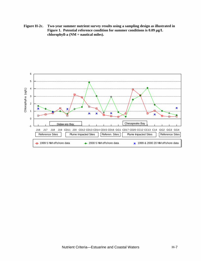
Nutrient Criteria—Estuarine and Coastal Waters H-7
-1
0
1
2
3
4
5
6
Chl
orop
hyll-
a (
ug/L
)
J16 J17 J18 J19 CD11 J20 CD12 CD13 CD14 CD15 CD16 GG1 CD17 CD20 CC12 CC13 C14 GG2 GG3 GG4
1999 5 NM offshore data 2000 5 NM offshore data 1999 & 2000 20 NM offshore data
Chesapeake BayDelaw are Bay
Reference Sites Plume Impacted Sites Referen. Sites Plume Impacted Sites Reference Sites
Figure H-2c. Two-year summer nutrient survey results using a sampling design as illustrated inFigure 1. Potential reference condition for summer conditions is 0.09 µg/Lchlorophyll-a (NM = nautical miles).

Nutrient Criteria—Estuarine and Coastal WatersH-8
-2
0
2
4
6
8
10
12
14
16
Sec
chi d
epth
(m
)
J16 J17 J18 J19 CD11 J20 CD12 CD13 CD14 CD15 CD16 GG1 CD17 CD20 CC12 CC13 C14 GG2 GG3 GG4
1999 5 NM offshore data 2000 5 NM offshore data
Delaw are Bay Chesapeake Bay
Reference Sites Plume Impacted Sites Referen. Sites Plume Impacted Sites Reference Sites
Figure H-2d. Two-year summer nutrient survey results using a sampling design as illustrated inFigure 1. Secchi depth data are incomplete because of missing observations duringnight-time operations (NM = nautical miles).

Nutrient Criteria—Estuarine and Coastal Waters H-9
Standard Methods persulfate digestion method. All samples were frozen on board for later analysis at theUniversity of Maryland Chesapeake Biological Laboratory. Secchi depth was determined using a 35 cmdiameter white Secchi disc on 0.5 m marked line.
ResultsPreliminary data analyses indicated that the groupings of two or three stations (originally intended toreflect progressive off shore encroachment of nutrient runoff) are not significantly different. Similarly,initial assessment of the surface, mid-depth, and bottom water column samples showed no significantdifferences for the nutrient criteria indicators except for DO. Salinity did show the expected surface tobottom variations expected of near coastal waters. Consequently horizontal and vertical samplingdistances for each station were combined to produce the nutrient results presented here.
The following figures illustrate the results of two summer surveys in 1999 and 2000. Data indicated byan asterisk represents the mean of combined two year data from each 20 nm off shore station. Gaps inthe Secchi depth results are because of the night time intervals during 24-hour operations. The stationslocated in the vicinity of the estuarine discharges of Delaware and Chesapeake Bays are indicated by theappropriately labeled open boxes, i.e. J18 through CD12 for the Delaware and CD17 through CC13 forthe Chesapeake.
Discussion• The survey technique appears to faithfully reflect the nutrient conditions of the coastline in that
higher nutrients were found in the waters just off each estuary. Further, when surface stationsalinity was plotted, a mirror image of the nutrient data results was presented indicating afreshwater correlation with higher nutrient concentrations. The biological response of the waterswas also evident from the correlation of Chl-a and SD data with the TN and TP levels.
• Given the variability in only two years of data, it is interesting that the offshore stations appear tobe relatively consistent in all three nutrient parameters. The incongruity of the TP and TN dataat GG1 for 1999 and for chlorophyll-a at CD16 for 2000 is also noted, but unexplained.
• The two consecutive sampling years demonstrated similar trends among the stations indicatingno major weather variability during this period and also suggesting that the proposed referencesites respond comparably to the discharge sites to inter-annual climatological events.
• The stations that consist of sets of two or three sites within a few miles of one another weredetermined upon review of the data to have very little distinction. This suggests thatperturbation, if any, originating from the coastal land mass has had an impact over all three sites.
• It appears that the Delaware plume drifts more southward from the mouth of its bay than does the
Chesapeake. This may reflect the lower discharge volume of the Delaware and the influence ofthe Hudson River discharge and Longshore current, both displacing the plume southward. Similarly, the slight northward offset of both the Delaware and Chesapeake plumes in 1999relative to 2000 may be a response to changing coastal current dynamics from year to year.
• There was no significant difference between the eight offshore sites (20 nm offshore) and theirinshore counterparts. Further comparison of offshore stations to those counterparts within theestuarine discharge plumes will help determine the sensitivity of the comparison. Theintermediate 10 nm stations do not appear to add substantial information and can be discontinuedexcept in the vicinity of discharge plumes to help define these margins.

Nutrient Criteria—Estuarine and Coastal WatersH-10
While the data is limited, it is encouraging that the offshore controls are comparable to theexpected inshore reference sites. Candidate inshore reference sites are initially selected on thebasis of an apparent physical absence of local cultural impact, i.e. tributary discharges, municipaldischarges, ports or marinas, or other commercial enterprises. Because of the potentially highvariability in the existing data, a concurrence between offshore and inshore reference stations isnot necessarily confirmation of the quality of the inshore reference sites, but when consistent with observed physical indications, this information adds confidence to the selection. Conversely, significant differences would be cause for suspecting the inshore site selection as ofreference quality.
• In this regard, an interesting trend was noted among the three groups of reference sites locatednorth of Delaware Bay; between Delaware and Chesapeake Bay; and south of Chesapeake Bay(Figures 2a-d). The mean ambient concentrations of TP, TN and Chlorophyll-a at thesereference sites trend downward from north to south. The same trend appears in the eightstations 20 nm offshore presumably reflecting a broad scale process affecting this area. Thisfurther supports the importance of establishing relatively close spaced reference sites whenpreparing coastal marine criteria The mean TP values for the nearshore reference sites at thenorthern terminus of the transect of stations is significantly higher than those at the southern end(p = 0.0006) even though the region is presumed to be geologically homogeneous.
• Secchi depth data were inconclusive because not enough data points were generated as aconsequence of 24-hour sampling when Secchi depth could not be determined during night-timehours. Additional future sampling will be conducted during daylight so all parameters may beevaluated.
Committee Discussion of the Prototype MethodologyFixed Station Sampling vs Stratified Random SamplingInferences derived from fixed-station and fixed-transect sampling, while common in oceanographicresearch and monitoring, are potentially confounded by unintentional and unknown biases, and by theinability to extend statistical inferences to the entire sample space desired. Alternatively, fixed stationstend to reduce the amount of unknown physical variability associated with interpreting climatic factorsupon a given site such as when attempting to assess hurricanes, upwelling or acid deposition effects on aparticular coastline. Although there is no reason to suspect that the existing stations of the mid-Atlanticcoastal nutrient study are biased, the design group thought that the design should allow data inference tothe entire coastal sampling space. It therefore proposes a change to a probability-based design, of equalsampling cost, to avoid the potential pitfalls of a fixed-station design.
The sample space for this project is open marine waters of the U.S. coastal zone, with emphasis on statewaters within the 3 nautical mile state limit. Sampling will be carried out in three sampling strata forwhich nutrient conditions are to be estimated:
1. Reference areas within the 3-mile limit, outside the influence of major estuary plumes (e.g.,Hudson River, Delaware Bay, Chesapeake Bay);
2. Nutrient influenced areas within the 3-mile limit, affected by the estuary plumes and otherdischarges; and
3. Offshore waters beyond the state 3-mile limit.

Nutrient Criteria—Estuarine and Coastal Waters H-11
These three regions will define the sampling strata. The sampling design will be to define longshore“cells” in each of these three zones. During each sampling event, one site will be selected randomlywithin each sampling cell. The overall design can be described as stratified-systematic-random; wherethe strata are the three areas defined by estuary influence and distance from shore, the systematiccomponent is the cells that define each stratum, and the random component is the random samplinglocation selected on each cell during each sampling event (Figure H-3).
The first task in developing the sampling plan will be to define areas of presumed estuarine influence,from existing physical oceanographic research on water movement, in this case in the mid-Atlanticcoastal area, and from existing water chemistry data showing elevated nutrients and other constituentssuch as salinity and conductivity in the estuary plumes. Because plumes will vary with estuarinedischarge, Gulf Stream eddies, and other events, precise definition of the plume area is not possible. Instead, plume areas should be defined as where the estuarine influence is likely to occur. Anunderstanding of local estuarine hydrology will help in this regard, but extensive and expensive physicalinvestigations should not be a prerequisite for the determination of likely plume influence.
Coastal reference site determinations and reference condition derivation should be, at least initially,established by EPA. Data collection would be continued as an EPA function because the offshorestations are the purview of the Federal government and because the related reference sites can beincorporated in the effort.
Estuarine and riverine plume monitoring are more likely accomplished by the coastal States usingexisting budgets and vessels already at their disposal. A coordinated effort relating State and Federalsampling and data exchange should be promoted. The nutrient quality of the discharge plumes can thenbe expeditiously compared to the proximal reference condition(s) to assess impact upon the near coastalmarine waters.
Regional coastal characteristics will determine both the reference site cell structures and placement andthe estuarine or riverine plume sampling designs.
Sampling Times and DepthsThe committee recommended that sampling be conducted during the period of optimal marine vegetativegrowth. In temperate areas this is Spring and Summer, generally May, June and July, August. Otherinterval options depending on locale might be wet and dry periods during the growing season.
As a cost effective approach producing scientifically valid results, sampling depth is recommended asalways at the surface, i.e., top meter of water accompanied by either a composite sample from theremainder of the water column or sampling from just below the thermocline and at one meter above thebottom. Some members of the committee advocate the surface, mid-depth, and bottom samplingtechnique where the mid-depth sample is usually below the thermocline and/or where inshore watersoften fail to demonstrate a thermocline.
VariablesThe primary four variables of TN, TP, Chlorophyll-a, and SD are recommended because they are the bestearly indicators of causal and biological response indicators to nutrient loadings. Other measures ofclarity or transparency may also be used, but Secchi depth should always be included because such alarge body of information is already available in this form; it is inexpensive and reliable; and continuedSecchi depth measurements provide a continuity with much historical data. In an independent

Nutrient Criteria—Estuarine and Coastal WatersH-12
UU
U U
lll
l
l
l
l
l
l
l
1 0 N M 2 0 N M
1 0 N M 2 0 N M
1 - 3 N M
A
B
C
D
E
Figure H-3. Illustration of stratified random grid sample design for reference condition cells asrelated to an estuarine discharge. Nutrient quality and spatial extent of the gridcan be compared to a value derived from the measurements in reference sites (cells)A-E. Values at 10 and 20 nm stations are a check against reference values found atA-E.

Nutrient Criteria—Estuarine and Coastal Waters H-13
investigation, the Swedish Environmental Protection Agency selected the same four primary variables(Report 5052, 2000). Other recommended variables are: dissolved oxygen as an important secondary response variable almostalways measured by investigators because of the significance of respiration to the biological community,and planktonic species composition as a refined diagnostic indicator of the nature and extent ofenrichment.
Geographic Application of the ProtocolMembers of the committee are familiar with both the East, West, and Gulf coasts of the continental U.S.and conclude that the method described above, with allowances for regional modifications such asrelative distance from shore to shelf break and the magnitude of upwelling, can be successfully applied inall three coastal environments to identify reference conditions for criteria development.
Summary Conclusions1. The basic protocol as described, but modified to include a probability-based sampling design, a
variation on the surface, mid-depth, and bottom sampling profile, and sampling emphasis ontwice during the growing season, is a scientifically defensible and broadly applicable method forestablishing regional reference conditions to support coastal marine nutrient criteriadevelopment.
2. The TP, TN, Chlorophyll-a, and perhaps Secchi depth variables are responsive and together withsalinity measurements are descriptive of both estuarine discharge plumes and near coastalreference quality waters. These measurements can be used to assess the concentration and areachanges of discharge plumes over time.
3. The comparison of marine nutrient water quality to inshore reference sites is valuable asconfirmation of “natural” reference conditions and as a graphic descriptor of the referenceconcept for the public. However, for cost effectiveness, these off shore stations need not bemonitored every time the inshore reference sites are sampled.
4. But it is important to note that the distinction of cultural from inherent nutrient discharges byestuaries and other tributaries to coastal waters is not possible just by comparison to referenceconditions. The other elements of nutrient criteria development should be incorporated to helpmake this distinction. The reference conditions and criteria will reveal exceedences of the“natural” background levels to be preferred and the relative extent and magnitude of the problem,but source identification and cause and effect studies will be required for an effectivemanagement response to this identified concern.

Nutrient Criteria—Estuarine and Coastal Waters R-1
REFERENCES
Alongi, DM. 1998. Coastal Ecosystem Processes. Boca Raton, FL: CRC Press.
Ambrose, RB, Jr, TA Wool, JL Martin. 1993. The Water Quality Analysis Simulation Program,WASP5. Part A: Model Documentation. U.S. Environmental Protection Agency, Office of Research andDevelopment, Environmental Research Laboratory, Athens, GA.
Anderson, DM. 2000. Symposium on harmful algae in the U.S. Symposium agenda, abstracts, andparticipants, Marine Biological Laboratory, Woods Hole, MA.
Anderson, DM, DJ Garrison, eds. 1997. The ecology and oceanography of harmful algal blooms. Limnol Oceanogr 42:1305.
Antia, NJ, PJ Harrison, L Oliveira. 1991. The role of dissolved organic nitrogen in phytoplanktonnutrition, cell biology, and ecology. Phycologia 30:1-89.
APHA (American Public Health Association). 1998. Standard Methods for the Examination of Waterand Wastewater, 20th ed. American Public Health Association, Washington, DC.
Asselin, S, ML Spaulding. 1993. Flushing times for the Providence River based on tracer experiments. Estuaries 16(4):830-839.
Atlas, RM, R Bartha. 1993. Microbial Ecology Fundamentals and Applications. Redwood City, CA: Benjamin/Cummings.
Azam, F, T Fenchel, JG Field, JS Gray, TA Meyer-Reil, F Thingstad. 1983. The ecological role ofwater-column microbes in the sea. Mar Ecol Prog Ser 10:257-263.
Batiuk, R, R Orth, K Moore, JC Stevenson, W Dennison, L Staver, V Carter, N Rybicki, R Hickman, SKollar, S Bieber. 1992. Submerged aquatic vegetation habitat requirements and restoration targets: atechnical synthesis. U.S. EPA, Chesapeake Bay Program, Annapolis, MD. CBP/TRS 83/92.
Batiuk, RA, P Bergstrom, M Kemp, E Koch, L Murray, JC Stevenson, R Bartleson, V Carter, NBRybicki, JM Landwehr, C Gallegos, L Karrh, M Naylor, D Wilcox, KA Moore, S Ailstock, M Teichberg. 2000. Chesapeake Bay submerged aquatic vegetation water quality and habitat-based requirements andrestoration targets: a second technical synthesis. Chesapeake Bay Program, Annapolis, MD. CBP/TRS245/00. EPA 903-R-00-014.
Behrenfeld, MJ, PG Falkowski. 1997. A consumer’s guide to phytoplankton primary productivitymodels. Limnol Oceanogr 42(7):1479-1491.
Bell, RG, DG Goring. 1998. Seasonal variability of sea level and sea-surface temperature on the north-east coast of New Zealand. Estuarine Coastal Shelf Sci 46:307-318.
Bernhard, AE, ER Peele. 1997. Nitrogen limitation of phytoplankton in a shallow embayment innorthern Puget Sound. Estuaries 20(4):759-769.
Bianchi, TS, JR Pennock, RR Twilley, eds. 1999. Biogeochemistry of Gulf of Mexico Estuaries. NewYork: John Wiley.

Nutrient Criteria—Estuarine and Coastal WatersR-2
Biggs, RB, DA Flemer. 1972. The flux of particulate carbon in an estuary. Marine Biol (Berlin) 12:11-17.
Billen, G, C Lancelot, M Meybeck. 1991. N, P, Si retention along the aquatic continuum from land toocean. In: RFC Mantoura, J-M Martin, R Wollast, eds. Ocean Margin Processes in Global Change. New York: John Wiley, pp. 19-44
Bledsoe, EL, EJ Phlips. 2000. Relationships between phytoplankton standing crop and physical,chemical, and biological gradients in the Suwannee River and Plume Region, U.S.A. Estuaries23(4):458-473.
Boicourt, WC. 1992. Influences of circulation processes on dissolved oxygen in the Chesapeake Bay. In: DE Smith, M Leffler, G Mackiernan, eds. Oxygen Dynamics in the Chesapeake Bay: A Synthesis ofResearch. Maryland Sea Grant College, College Park, MD, pp. 7-60.
Bolin, B, H Rodhe. 1973. A note on the concepts of age distribution and transit time in naturalreservoirs. Tellus 25(1):58-62.
Boynton, WR. 1997. Potomac River integrated analysis project. Chesapeake Biological Laboratory,University of Maryland, Solomons, MD.
Boynton, WR, JH Garber, R Summers, WM Kemp. 1995. Inputs, transformations, and transport ofnitrogen and phosphorus in Chesapeake Bay and selected tributaries. Estuaries 18(1B):285-314.
Boynton, WR, JD Hagy, L Murray, C Stokes, WM Kemp. 1996. A comparative analysis ofeutrophication patterns in a temperate coastal lagoon. Estuaries 19(2B):408-421.
Boynton, WR, WM Kemp. 2000. Influence of river flow and nutrient loads on selected ecosystemprocesses: a synthesis of Chesapeake Bay data. In: JE Hobbie, ed. Estuarine Science: A SyntheticApproach to Research and Practice. Washington, DC: Island Press, pp. 269-298.
Boynton, WR, WM Kemp, CW Keefe. 1982. A comparative analysis of nutrients and other factorsinfluencing estuarine phytoplankton production. In: V Kennedy, ed. Estuarine Comparisons. SanDiego: Academic Press.
Brandes, JA, AH Devol. 1995. Simultaneous oxygen and nitrate respiration in coastal sediments:evidence for discrete diagenesis. J Mar Res 5:771-797.
Breitburg, DL, JG Sanders, CC Gilmour, CA Hatfield, RW Osman, GF Riedel, SP Seitzinger, KGSellner. 1999. Variability in responses to nutrients and trace elements, and transmission of stressoreffects through an estuarine food web. Limnol Oceanogr 44(3,2):837-863.
Bricker, SB, CG Clement, DE Pirhalla, SP Orlando, DRG Farrow. 1999. National estuarineeutrophication assessment: effects of nutrient enrichment in the Nation’s estuaries. NOAA, NationalOcean Service, Special Projects Office, and the National Centers for Coastal Ocean Science, SilverSpring, MD.
Brooks, DA, MW Baca, Y-T Lo. 1999. Tidal circulation and residence time in a macrotidal estuary:Cobscook Bay, Maine. Estuarine Coastal Shelf Sci 49:647-665.

Nutrient Criteria—Estuarine and Coastal Waters R-3
Brown, WS, E Arellano. 1980. The application of a segmented tidal mixing model to the Great BayEstuary, NH. Estuaries 3(4):248-257.
Brush, GS. 1984. Statigraphic evidence of eutrophication in an estuary. Water Res 20(5):531-541.
Brush, GS. 1986. Geology and paleoecology of Chesapeake Bay: a long-term monitoring tool formanagement. J Wash Acad Sci 76(3):146-160.
Brush, GS. 1992. A stratigraphic study of Perdido Bay. Florida Dept. of Geography and EnvironmentalEngineering, Johns Hopkins University, Baltimore, MD.
Buchak, EM, Edinger, JE. 1984a. Generalized, longitudinal-vertical hydrodynamics and transport: development, programming and applications. U.S. Army Corps of Engineers, WES, Vicksburg, MS,June 1984. Document No 84-18-R.
Buchak, EM, Edinger, JE. 1984b. Simulation of a density underflow into Wellington Reservoir usinglongitudinal-vertical numerical hydrodynamics. U.S. Army Corps of Engineers, WES, Vicksburg, MS,March 1984. Document No 84-18-R.
Cai, W-J, LR Pomeroy, MA Moran, Y Wang. 1999. Oxygen and carbon dioxide mass balance for theestuarine-intertidal marsh complex of five rivers in the southeastern U.S. Limnol Oceanogr 44(3):639-649.
Callaway, RJ. 1981. Flushing study of South Beach Marina, Oregon. J Waterway, Port, Coastal andOcean Div. ASCE 107(WW2):47-58.
Cambell, RC. 1989. Statistics for Biologists. 3rd ed. Cambridge: Cambridge University Press.
Canfield, DE. 1993. Organic matter oxidation in marine sediments. Interactions of C, N, P, and Sbiogeochemical cycles. In: R Wollast, L Chou, F Mackenzie, eds. New York: Springer-Verlag, pp. 333-363.
Capper, J, G Power, FR Shivers, Jr. 1983. Chesapeake Waters: Pollution, Public Health, and PublicOpinion, 1607-1972. Centreville, MD: Tidewater Publishers.
Caraco, N, JJ Cole, GE Likens. 1990. A comparison of phosphorus immobilization in sediments offreshwater and coastal marine systems. Biogeochemistry 9:277-290.
Carlson, P, E Graneli. 1993. Availability of humic bound nitrogen for coastal phytoplankton. EstuarineCoastal Shelf Sci 36:433-447.
Carpenter, SR, NF Caraco, DL Correll, RW Howarth, AN Sharpley, VH Smith. 1998. Nonpointpollution of surface waters with phosphorus and nitrogen. Ecol Appl 8(3):559-568.
Carpenter, SR, JF Kitchell, JR Hodgson. 1985. Cascading trophic interactions and lake productivity. Bioscience 35:364-369.
Carriker, MR. 1967. Ecology of estuarine benthic invertebrates: a perspective. In: GH Lauff, ed. Estuaries. Washington, DC: American Association for the Advancement of Science, Publication 83, pp.442-487.

Nutrient Criteria—Estuarine and Coastal WatersR-4
Carter, HH, RJ Regier, EW Schniemer, JA Michael. 1978. The summertime vertical distribution ofdissolved oxygen at the Calvert Cliffs generating station: a physical interpretation. Chesapeake BayInstitute, The Johns Hopkins University, Special Report 60.
Cerco, CF, T Cole. 1995. User’s Guide to the CE-QUAL-ICM. Release Version 10. Technical ReportEL-95-1, U.S. Army Engineer Waterways Experiment Station, Vicksburg, MS.
Champ MA, GA Gould, III, WE Bozzo, SG Ackleson, KC Vierra. 1980. Characterization of lightextinction and attenuation in Chesapeake Bay, August, 1977. In: VS Kennedy, ed. EstuarinePerspectives. New York: Academic Press, pp. 263-277.
Chen, R, RR Twilley. 1999. Patterns of mangrove forest structure and soil nutrient dynamics along theShark River Estuary, Florida. Estuaries 22(4):955-970.
Christiansen, JP, JW Murray, AH Devol, LA Codispoti. 1987. Denitrification in continental shelfsediment has major impact on oceanic nitrogen budget. Global Biogeochem Cycles 1:97-116.
Cifuentes, LA, LE Schemel, JH Sharp. 1990. Qualitative and numerical analyses of the effects of riverinflow variations on mixing diagrams in estuaries. Estuarine Coastal Shelf Sci 30:411-427.
Clark, GM, DK Mueller, MA Mast. 2000. Nutrient concentrations and yields in undeveloped streambasins of the United States. J Am Water Res Assoc 36:849-860.
Clarke, KR, RM Warwick. 1994a. Change in Marine Communities: An Approach to Statistical Analysisand Interpretation. Natural Environment Research Council, Plymouth Marine Laboratory, Plymouth,England.
Clarke, KR, RM Warwick. 1994b. Similarity-based testing for community pattern: the two-way layoutwith no replication. Mar Biol 118:167-176.
Cloern, JE. 1982. Does the benthos control phytoplankton biomass in south San Francisco Bay (USA)? Mar Ecol Prog Ser 9:191-202.
Cloern, JE. 1996. Phytoplankton bloom dynamics in coastal ecosystems: a review with some generallessons from sustained investigation of San Francisco Bay, California. Rev Geophys 34(2):127-168.
Cloern, JE. 1999. The relative importance of light and nutrient limitation of phytoplankton growth: asimple index of coastal ecosystem sensitivity to nutrient enrichment. Aquat Ecol 33:3-16.
Cloern, JE. 2001. Our evolving conceptual model of the coastal eutrophication problem. Mar Ecol ProgSer 210:223-253.
Cloern, JE, AE Alpine, BE Cole, RIJ Wong, JF Arthur, MD Ball. 1983. River discharge controlsphytoplankton dynamics in the northern San Francisco Bay estuary. Estuarine Coastal Shelf Sci 16:415-529.
Colwell, RR. 1996. Global climate and infectious disease: the Colera paradigm. Science 274:2025-2031.

Nutrient Criteria—Estuarine and Coastal Waters R-5
Conley, DJ. 2000. Biogeochemical nutrient cycles and nutrient management strategies. Hydrobiologia419:87-96.
Conley, DJ, TC Malone. 1992. Annual cycle of dissolved silicate in Chesapeake Bay: implications forthe production and fate of phytoplankton biomass. Mar Ecol Prog Ser 81:121-128.
Conley, DJ, CL Shelske, EF Stoermer. 1993. Modification of the biogeochemical cycle of silica witheutrophication. Mar Ecol Progr Ser 101:179-192.
Cooper, SR. 1995. Chesapeake Bay watershed historical land use: impact on water quality and diatomcommunities. Ecol Appl 5:703-723.
Cornwell, JC, WM Kemp, TM Kana. 1999. Denitrification in coastal ecosystems: methods,environmental controls, and ecosystem level controls, a review. Aquat Ecol 33:41-54.
Costa, JE. 2000. Managing anthropogenic nitrogen inputs to coastal embayments: technical basis andevaluation of a management strategy adopted for Buzzards Bay: Supplementary information on waterquality and habitat goals Buzzards Bay Project.
Costa, JE, BL Howes, D Janik, D Aubrey, E Gunn, AE Giblin. 1999. Managing anthropogenic nitrogeninputs to coastal embayments: technical basis and evaluation of a management strategy adopted forBuzzards Bay, Buzzards Bay Project.
Courtemanch, DC, SP Davies, EP Laverty. 1989. Incorporation of biological information in waterquality planning. Environ Manage 13:35-41.
D’Elia, CF, DM Nelson, WR Boynton. 1983. Chesapeake Bay nutrient and plankton dynamics. III. The annual cycle of dissolved silica. Geochim Cosmochim Acta 47:1945-1955.
D’Elia, CF, JG Sanders, WR Boynton. 1986. Nutrient enrichment studies in a coastal plain estuary:phytoplankton growth in large-scale, continuous cultures. Can J Fish Aquat Sci 43:397-406.
Day, JW Jr, CAS Hall, WM Kemp, A Yanez-Arancibia. 1989. Estuarine Ecology. New York: JohnWiley.
Dennison, WC, RJ Orth, KA Moore, JC Stevenson, V Carter, S Kollar, PW Bergstrom, RA Batiuk. 1993. Assessing water quality with submersed aquatic vegetation. Habitat requirements as barometersof Chesapeake Bay health. Bioscience 43:86-94.
Dettmann, EH. In press. Effect of water residence time on average concentrations, denitrification, andexport of nitrogen in estuaries: a model analysis. Estuaries.
Dettmann, EH, WA Brown, WM Warren, MF Fox, DR Kester. 1992. Final report on application of awasteload allocation model to multiple discharge sources into an estuary US Environmental ProtectionAgency Report. Narragansett, RI: Environmental Protection Agency. EPA/600/X-92/026.
Dettmann, EH, JF Paul, JS Rosen, CJ Strobel. 1989. Transport, fate and toxic effects of a sewagetreatment plant effluent in a Rhode Island estuary. U.S. Environmental Protection Agency. Narragansett,RI. EPA/600/X-89/062.

Nutrient Criteria—Estuarine and Coastal WatersR-6
Devol, AH, LA Codispoti, JC Christensen. 1997. Summer and winter denitrification rate in westernArctic shelf sediments. Cont Shelf Res 9:1029-1050.
Diaz, RJ, R Rosenberg. 1995. Marine benthic hypoxia: a review of its ecological effects and thebehavioral responses of benthic macrofauna. Oceanogr Mar Biol Ann Rev 33:245-303.
Digby, PGN. 1987. Multivariate Analysis of Ecological Communities. New York: Chapman and Hall.
Dixon, LK, GJ Kirkpatrick. 1999. Causes of light attenuation with respect to seagrasses in the upper andlower Charlotte Harbor. Mote Marine Laboratory Technical Report No. 650. Sarasota, FL.
Doering, PH, CA Oviatt, MEQ Pilson. 1990. Control of nutrient concentrations in the Seekonk-Providence River region of Narragansett Bay, Rhode Island. Estuaries 13(4):418-430.
Dortch, Q, ML Parsons, NN Rabalais, RE Turner. 1998. What is the threat of harmful algal blooms inLouisiana coastal waters? In: LP Rozas, JA Nyman, CE Profitt, NN Rabalais, DJ Reed, RE Turner, eds. From Symposium, Recent Research in Coastal Louisiana, 3-5 February 1998, Lafayette, LA.
Downing, JA. 1997. Marine nitrogen: Phosphorus stoichiometry and the global N:P cycle. Biogeochemistry 37:237-252.
Dronkers, J. 1988. Coastal-Offshore Ecosystem Interactions. Berlin: Springer-Verlag.
Duarte, CM. 1995. Submerged aquatic vegetation in relation to different nutrient regimes. Ophelia 41:87-112.
Dyer, K. 1973. Estuaries: A Physical Introduction. New York: Wiley-Interscience.
Dyer, KR, PA Taylor. 1973. A simple, segmented prism model of tidal mixing in well-mixed estuaries. Estuarine Coastal Mar Sci 1:411-418.
Eckblad, JW. 1991. How many samples should be taken? BioScience 41(5):346-348.
Edinger, JE, EM Buchak. 1983. Developments in LARM2: A longitudinal-vertical, time-varyinghydrodynamic reservoir model USAE Waterways Experiment Station, Vicksburg, MS. Technical ReportE-83-1.
ELI (Environmental Law Institute). 1988. Almanac of Enforceable State Laws to Control NonpointSource Water Pollution. Washington, DC. ELI Project # 970301.
Elmgren, R, U Larsson. 1997. Himmerfjarden: forandringer i ett naringsbelastat kustekyosystem iOsterjon. Rapport 4565. Naturvardsverket Forlag.
Emerson, K, RC Russo, RE Lund, RV Thurston. 1975. Aqueous ammonia equilibrium calculations:effect of pH and temperature. J Fish Res Bd Can 32:2379-2383.
Ennis, GP. 1986. Stock definition, recruitment variability, and larval recruitment processes in theAmerican lobster, Homarus americanus: a review. Can J Fish Aquat Sci 43:2072-2084.

Nutrient Criteria—Estuarine and Coastal Waters R-7
Environmental and Hydraulics Laboratories. 1986. CE-QUAL-W2, A Numerical Two-Dimensional,Model of Hydrodynamics and Water Quality, User's Manual, USACE Waterways Experiment Station,Vicksburg, MS. Instruction Report E-86-5.
Eppley, RW. 1972. Temperature and phytoplankton growth in the sea. Fish Bull 70(4):1063-1085.
Evans-Hamilton, Inc. 1998. Budd Inlet Scientific Study – Final Report. Prepared for: The Lacey,Olympia, Tumwater, Thurston County Partnership (LOTT), Seattle, WA.
Eyre, B, P Balls. 1999. A comparative study of nutrient behavior along the salinity gradient of tropicaland temperate estuaries. Estuaries 22(2A):313-326.
Fairweather, PG. 1991. Statistical power and design requirements for environmental monitoring. Austral J Mar Freshw Res 42:555-567.
Fisher, TR, LW Harding, Jr, DW Stanley, LG Ward. 1988. Phytoplankton, nutrients, and turbidity in theChesapeake, Delaware, and Hudson estuaries. Estuarine Coastal Shelf Sci 27:61-93.
Fisher, TR, ER Peele, JW Ammerman, LW Harding, Jr. 1992. Nutrient limitation of phytoplankton inChesapeake Bay. Mar Ecol Prog Ser 82:51-63.
Flemer, DA. 1970. Primary production in Chesapeake Bay. Chesapeake Sci 11:117-129.
Flemer, DA, EM Lores, CM Bundrick. 1998. Potential sediment denitrification rates in estuaries ofnorthern Gulf of Mexico. J Environ Qual 27(4):859-869.
Flemer, DA, GB Mackiernan, W Nehlsen, VK Tippie, et al. 1983. Chesapeake Bay: A Profile ofEnvironmental Change. US EPA, Region 3, Philadelphia, PA, plus Appendices A-D.
Flint, RW. 1985. Long-term estuarine variability and associated biological response. Estuaries8(A):158-169 .
Fourqurean, JW, JC Zieman, GVN Powell. 1992a. Phosphorus limitation of primary production inFlorida Bay: evidence from the C:N:P ratios of the dominant seagrass, Thalassia testudinum. LimnolOceanogr 37:162-171.
Fourqurean, JW, JC Zieman, GVN Powell. 1992b. Relationships between porewater nutrients andseagrasses in a subtropical carbonate environment. Mar Biol 114:57-65.
Fulmer, DG, GD Cooke. 1990. Evaluating the restoration potential of nineteen Ohio reservoirs. LakeReservoir Manage 6:197-206.
Funderburk, SL, SJ Jordan, JA Mihursky, DR Riley, eds. 1991. Habitat Requirements for ChesapeakeBay Living Resources, 1991 Revised Edition. Living Resources Subcommittee, Chesapeake BayProgram, Annapolis, MD.
Gallegos, CL. 1994. Refining habitat requirements of submersed aquatic vegetation: role of opticalmodels. Estuaries 17(1B):187-199.

Nutrient Criteria—Estuarine and Coastal WatersR-8
Gallegos, CL, TE Jordan. 1997. Seasonal progression of factors limiting phytoplankton pigmentbiomass in the Rhode River estuary, Maryland (USA). I. Controls on phytoplankton growth. Mar EcolProg Ser 168:185-198.
Gerlach, SA. 1990. Stickstoff, phosphor, plankton, und sauerstoff mangel in der Deutchen Bucht und inder Kieler Bucht Abschlussbericht uber das Teilvorhaben 9, Koordination, im Rahmen desForschungsbericht. 102 04 215. UBA-FB 89-083. Berlin: Erich Schmidt Verlag.
Geyer, WR. 1997. Influence of wind on dynamics and flushing of shallow estuaries. Estuarine CoastalShelf Sci 44:713-722.
Geyer, WR, JT Morris, FG Prahal, DA Jay. 2000. Interaction between physical processes and ecosystemstructure, Chapter 8. In: JE Hobbie, ed. Estuarine Science—A Synthetic Approach to Research andPractice. Washington, DC: Island Press, pp. 177-206.
Geyer, WR, P Dragos, T Donoghue. 1997. Flushing studies of three Buzzards Bay harbors: Onset Bay,Little Bay, and Allen's Pond Report prepared for the Buzzard Bay Project, Marion, MA (now located inWareham, MA).
Gibson, G, R Wedepohl, D Knaver. 1983. Lake protection by watershed management for Wisconsinlake districts. Proceedings of the North American Lake Management Society, Vancouver, BC, Canada. EPA 44015-83-001.
Giller, PS, AG Hildrew, DG Raffaelli. 1994. Aquatic Ecology—Scale, Pattern, and Process. Oxford:Blackwell Scientific Publications.
Goldman, JC, JJ McCarthy, DG Peavey. 1979. Growth rate influence on the chemical composition ofphytoplankton in oceanic waters. Nature 279(17 May):210-215.
Greening, HS, G Morrison, RM Eckenrod, MJ Perry. 1997. The Tampa Bay resource-basedmanagement approach. In: SF Treat, ed. Proceedings, Tampa Bay Area Scientific InformationSymposium 3: Applying Our Knowledge. Tampa Bay Estuary Program, St Petersburg, FL. pp. 349-355.
Guilford, SJ, RE Hecky. 2000. Total nitrogen, total. phosphorus, and nutrient limitation in lakes andoceans: Is there a common relationship? Limnol Oceanogr 45(6):1213-1223.
Hagy, JD, LP Sanford, WR Boynton. 2000. Estimation of net physical transport and hydraulic residencetimes for a coastal plain estuary using box models. Estuaries 23(3):328-340.
Hamrick, JM. 1996. A User’s Manual for the Environmental Fluid Dynamics Computer Code (EFDC). The College of William and Mary, Virginia Institute of Marine Science. Gloucester Point, VA. SpecialReport 331.
Hansen, DV, M Rattray. 1966. New dimensions in estuary classification. Limnol Oceanogr 11:319-326.
Harding, LW, Jr. 1994. Long-term trends in the distribution of phytoplankton in Chesapeake Bay: rolesof light, nutrients, and streamflow. Mar Ecol Prog Ser 104:267-291.
Harding, LW, ES Perry. 1997. Long-term increase of phytoplankton biomass in Chesapeake Bay, 1950-1994. Mar Ecol Prog Ser 157:39-52.

Nutrient Criteria—Estuarine and Coastal Waters R-9
Harris, GP. 1986. Phytoplankton Ecology—Structure, Function, and Fluctuations. New York: Chapmanand Hall.
Hass, LW. 1977. The effect of the spring-neap tidal cycle on the vertical salinity structure of the James,York, and Rappahannock rivers, Virginia, USA. Estuarine Coastal Mar Sci 5:485-496.
Hassett, RP, B Cardinale, LB Stabler, JJ Elser. 1997. Ecological stoichiometry of N and P in pelagicecosystems: comparion of lakes and oceans with emphasis on the zooplankton-phytoplanktoninteraction. Limnol Oceanogr 42(4):638-662.
Havens, KE. 1999. Correlation is not causation: a case study of fisheries, trophic state and acidity inFlorida (USA) lakes. Environ Pollut 106:1-4.
Hedges, JI, JH Stern. 1984. Carbon and nitrogen determinations of carbonate containing solids. LimnolOceanog 29:657-663.
Helder, W, RTP de Vries. 1983. Estuarine nitrite maxima and nitrifying bacteria (Elms-Dollardestuary). Netherlands J Sea Res 17:1-18.
Hirsch, RM, JR Slack, RA Smith. 1982. Techniques in trend analysis for monthly water quality data. Water Res 18:107-121.
Hobbie, JE, ed. 2000. Estuarine Science—a Synthetic Approach to Research and Practice. Washington,DC: Island Press.
Holland, AF, NK Mountford, JA Mihursky. 1977. Temporal variation in the upper bay mesohalinebenthic communities: 1. The 9-m mud habitat. Chesapeake Sci 18:370-378.
Holland, AF, AT Shaughnessy, MH Hiegel. 1987. Long-term variation in mesohaline Chesapeake Baymacrobenthos: spatial and temporal patterns. Estuaries 10(3):227-245.
Holmes, RW. 1970. The Secchi disk in turbid coastal waters. Limnol Oceanogr 15:688-694.
Hopkinson, CS, RL Wetzel. 1982. In situ measurements of nutrient and oxygen fluxes in a coastalmarine benthic community. Mar Ecol Progr Ser 10:29-35.
Howarth, R. 1988. Nutrient limitation of net primary production in marine ecosystems. Ann Rev Ecol19:89-110.
Howarth, RW, G Billen, D Swaney, A Townsend, N Jaworski, K Lajtha, JA Downing, R Elmgren, NCaraco, T Jordan, F Berendse, J Freney, V Kudeyarov, P Murdoch, Z Zhao-Liang. 1996. Regionalnitrogen budgets and riverine N&P fluxes, for drainages to the North Atlantic Ocean: natural and humaninfluences. Biogeochemistry 35:75-79.
Howarth, RW, HS Jensen, R Marino, H Postma. 1995. Transport to and processing of phosphorus innear-shore and oceanic waters. In: H Tiessen ed. Phosphorus in the Global Environment. New York:John Wiley.
Huisman, J. 1999. Population dynamics of light-limited phytoplankton: microcosm experiments. Ecology 80(1):202-210.

Nutrient Criteria—Estuarine and Coastal WatersR-10
Huisman, J, RR Jonker, C Zonneveld, FJ Weissing. 1999. Competition for light between phytoplanktonspecies: experimental tests of mechanistic theory. Ecology 80(1):211-222.
Jackson, JBC, MX Kirby, WH Berger, et al. 2001. Historical overfishing and recent collapse of coastalecosystems. Science 293(July):629-638.
Janicki, A, D Wade. 1996. Estimating critical external nitrogen loads for the Tampa Bay Estuary: anempirically based approach to setting management targets. Tampa Bay National Estuary Program, St.Petersburg, FL. Technical Publ # 06-96.
Jansson, B-O, K Dahlberg. 1999. The environmental status of the Baltic Sea in the 1940s, today, and inthe future. Ambio 28(4):312-319.
Jaworski, NA, RW Howarth, LJ Hetling. 1997. Atmospheric deposition of nitrogen oxides onto thelandscape contributes to coastal eutrophication in the northeast United States. Environ Sci Technol31:1995-2004.
Jay, DA, WR Geyer, DR Montgomery. 2000. An ecological perspective on estuarine classification. In:JE Hobbie, ed. Estuarine Science—A Synthetic Approach to Research and Practice. Washington, DC: Island Press.
Jeffery, SW, RFC Mantoura, SW Wright. 1997. Phytoplankton Pigments in Oceanography. Monographs in Oceanographic Methods. Paris, UNESCO.
Jenkins, MC, WM Kemp. 1984. The coupling of nitrification and denitrification in two estuarinesediments. Limnol Oceanogr 29:609-619.
Johnson, BH, RE Heath, BB Hsieh, KW Kim, HL Butler. 1991. User’s Guide for a Three-Dimensional,Numerical Hydrodynamic, Salinity, and Temperature Model of Chesapeake Bay. U.S. Army EngineerWaterways Experiment Station, Vicksburg, MS.
Jonas, R. 1992. Microbial processes, organic matter and oxygen demand in the water column. In: DSmith, M Leffler, G Mackiernan, eds. Dissolved Oxygen in Chesapeake Bay. Maryland Sea Grant,College Park, MD. pp. 113-148.
Josefson, AB, B Rasmussen. 2000. Nutrient retention by benthic macrofaunal biomass of Danishestuaries: importance of nutrient load and residence time. Estuarine Coastal Shelf Sci 50(2):205-216.
Justic, D. 1987. Long-term eutrophication of the Northern Adriatic Sea. Mar Pollut Bull 18(6):281-284.
Kannerworff, E, W Nicolaisen. 1973. The “Haps”: a frame-supported bottom corer. Ophelia 10:119-129.
Karr, JR. 1981. Assessment of biotic integrity using fish communities. Fisheries 6:21-27.
Keefe, CW, DA Flemer, DH Hamilton. 1976. Seston distribution in the Patuxent River Estuary. Chesapeake Sci 17:55-59.
Kelly, JR. 1998. Quantification and potential role of ocean nutrient loading to Boston Harbor,Massachusetts, USA. Mar Ecol Prog Ser 173:53-65.

Nutrient Criteria—Estuarine and Coastal Waters R-11
Kelly, JR. In press. Nitrogen effects on coastal marine ecosystems, Chapter 9. In: RF Follett, JLHatfield, eds. Nitrogen in the Environment: Sources, Problems, and Management. The Netherlands:Elsevier Publishers.
Kemp, WM, S Ailstock, R Batiuk, R Bartleson, P Bergstrom, V Carter, C Gallegos, W Hunley, L Karrh,EW Koch, J Landwehr, K Moore, L Murray, M Naylor, N Rybicki, JC Stevenson, D Wilcox. In Review. Habitat requirements for submerged aquatic vegetation in Chesapeake Bay: water quality, light regime,and physical-chemical factors.
Kemp, WM, WR Boynton, RR Twilley, JC Stevenson, JC Means. 1983. The decline of submergedvascular plants in upper Chesapeake Bay: summary of results concerning possible causes. Mar Tech Soc J 17:78-89.
Kemp, WM, WR Boynton. 1984. Spatial and temporal coupling of nutrient inputs to estuarine primaryproduction: the role of particulate transport and decomposition. Bull Mar Sci 35(3):522-535.
Kennedy, VS, ed. 1984. The Estuary as a Filter. New York: Academic Press.
Kennish, MJ. 1989. Practical Handbook of Marine Science. CRC Press.
Ketchum, BH. 1951. The exchanges of fresh and salt waters in tidal estuaries. J Mar Res 10(1):18-38.
Kierstead, H, LB Slobodkin. 1953. The size of water masses containing plankton blooms. J Mar Res12:141-147.
Kinne, O. 1964. The effects of temperature and salinity on marine and brackish water animals. II. Salinity and temperature salinity combinations. Oceanogr Mar Biol Ann Rev 2:281-339.
Kirk, JTO. 1983. Photosynthesis in Aquatic Ecosystems. Cambridge University Press.
Kjerfve, B. 1989. Estuarine geomorphology and physical oceanography. In: JW Day, Jr, CAS Hall,WM Kemp, A Yanez-Arancibia, eds. Estuarine Ecology. New York: John Wiley.
Knowlton, MF, JR Jones. 1989. Comparison of surfaces and depth integrated composite samples forestimating algal biomass and phosphorus values and notes on the vertical distribution of autotrophs inMidwestern lakes. Arch Hydrobiol 83(Suppl):175-196.
Koch, E.W. 2001. Beyond light: physical, geological, and geochemical parameters as possible submersedaquatic vegetation habitat requirements. Estuaries 24(1):1-17.
Koenigs, JP, JA Edmundson. 1991. Secchi disk and photometer estimates of light regimes in Alaskanlakes: effects of yellow color and turbidity. Limnol Oceanogr 36(1):91-105.
Lambourn, LD, AH Devol, JW Murray. 1991. R/V New Horizon 90-5 cruise report: water column andporewater data. Univ. Washington.
Lampman, GG, NF Caraco, JJ Cole. 1999. Spatial and temporal patterns of nutrient concentration andexport in the tidal Hudson River. Estuaries 22(2A):285-296.

Nutrient Criteria—Estuarine and Coastal WatersR-12
Lebo, ME, JH Sharp. 1993. Distribution of phosphorus along the Delaware, an urbanized coastal plainestuary. Estuaries 16(2):290-301.
Lee, GF, RA Jones. 1981. Application of the OECD eutrophication modeling approach to estuaries. In:Neilson, BJ, LE Cronin 1981, eds. Estuaries and Nutrients. Clifton, NJ: Humana Press, pp. 549-568.
Lehman, PW. 2000. The influence of climate on phytoplankton community biomass in San FranciscoBay Estuary. Limnol Oceanogr 45(3):580-590.
Lenihan, H, CH Peterson. 1998. How habitat degradation through fishery disturbance enhances impactsof oyster reefs. Ecol Appl 8:128-140.
Likens. 1992. The Ecosystem Approach: Its Use and Abuse. Oldendorf/Luhe, Germany: EcologyInstitute.
Lippson, AJ, MS Haire, AF Holland, et al. 1979. Environmental Atlas of the Potomac Estuary. Maryland Department of Natural Resources, Annapolis, MD.
Livingston, RJ. 1997. Trophic response of estuarine fishes to long-term changes of river runoff. BullMar Sci 60(3):984-1004.
Livingston, RJ. 2001a. Eutrophication Processes in Coastal Systems. Boca Raton, FL: CRC Press.
Livingston, RJ. 2001b. Nutrient loading and coastal plankton blooms: Seasonal/interannual successionsand effects on secondary production. Proceedings, IEEE International Symposium, Honolulu, Hawaii, 5-8 November 2001.
Lorenzen, CJ. 1972. Extinction of light in the ocean by phytoplankton. J Conservation 34:262-267.
Lucas, LV, JR Koseff, SG Monismith, et al. 1999. Processes governing phytoplankton blooms inestuaries. II. The role of horizontal transport. Mar Ecol Prog Ser 187:17-30.
Ludwig, JA, JF Reynolds. 1988. Statistical Ecology. New York: John Wiley.
Luepke, N-P. 1979. Monitoring Environmental Materials and Specimen Banking. Boston: MartinusNijhoff Publishers.
Magnien, RE, RM Summers, KG Sellner. 1992. External nutrient sources, internal nutrient pools, andphytoplankton production in Chesapeake Bay. Estuaries 15(4):497-516.
Mallin, MA, LB Cahoon, MR McIver, DC Parsons, GC Shank. 1999. Alteration of factors limitingphytoplankton production in the Cape Fear River Estuary. Estuaries 22(4):825-836.
Malone, TC, A Malej, LW Harding, Jr, N Smodlaka, RE Turner, eds. 1999. Coastal and EstuarineStudies, Ecosystems at the Land-Sea Margin, Drainage Basin to Coastal Sea, 55, American GeophysicalUnion, Washington, DC.
Malone, TC, DJ Conley, TR Fisher, PM Gilbert, LW Harding, KG Sellner. 1996. Scales of nutrient-limited phytoplankton productivity in Chesapeake Bay. Estuaries 19(2B):371-385.

Nutrient Criteria—Estuarine and Coastal Waters R-13
Malone, TC, LH Crocker, SE Pike, BW Wendler. 1988. Influences of river flow in the dynamics ofphytoplankton production in a partially stratified estuary. Mar Ecol Prog Ser 48:235-249.
Malone, TC, WM Kemp, HW Ducklow, WR Boynton, JH Tuttle, RB Jonas. 1986. Lateral variation inthe production and fate of phytoplankton in a partially stratified estuary. Mar Ecol Prog Ser 32:149-160.
Manahan, SE. 1997. Environmental Science and Technology. Boca Raton and New York: LewisPublishers.
Martin, JL, PF Wang, T Wool. 1996. A mechanistic management-oriented water quality model forTampa Bay. Surface Water Improvement and Management Department, Southwest Florida WaterManagement District, Tampa, FL.
McComb, AJ, R Humphries. 1992. Loss of nutrients from catchments and their ecological impacts inthe Peel-Harvey estuarine system, Western Australia. Estuaries 15:529-537.
Meybeck, M. 1982. Carbon, nitrogen, and phosphorus transport by world rivers. Am J Sci 282:401-450.
Miller, MW, ME Hay, SL Miller, D Malone, EE Sotka, AM Szmant. 1999. Effects of nutrients versusherbivores on reef algae: a new method for manipulating nutrients on coral reefs. Limnol Oceanogr44(8):1847-1861.
Miller, RL, BF McPherson. 1991. Estimating estuarine flushing and residence times in CharlotteHarbor, Florida, via salt balance and a box model. Limnol Oceanogr 36(3):602-612.
Millero, FJ. 1996. Chemical Oceanography. 2nd Ed. Marine Science Series. CRC Press.
Mills, EL. 1989. Biological Oceanography—An Early History. Ithaca: Cornell University Press.
Mills, WB, Porcella, DB, Ungs, MJ, Gherini, SA, Summers, KV, Lingfung, M, Rupp, GL, Bowie, GL,Haith, DA. 1985. Water Quality Assessment: A Screening Procedure for Toxic and ConventionalPollutants. U.S. Environmental Protection Agency, Athens, GA. EPA/600/6-85/002a,b.
Monbet, Y. 1992. Control of phytoplankton biomass in estuaries: a comparative analysis of microtidaland macrotidal estuaries. Estuaries 15:563-571.
Moore, KA, RL Wetzel. 2000. Seasonal variations in eelgrass (Zostera marina L). Responses tonutrient enrichment and reduced light availability in experimental ecosystems. J Exp Mar Biol Ecol244:1-28.
Muir, WC. 2001. USEPA Region III. Regional Office, Philadelphia, PA.
NALMS (North American Lake Management Society). 1992. Developing eutrophication standards forlakes and reservoirs. Alachua Press.
NAS (National Academy of Sciences). 1970. Eutrophication: causes, consequences, correctives. Proceedings of a symposium. Washington, DC.
Neilson, BJ, LE Cronin, eds. 1981. Estuaries and Nutrients. Clifton, NJ: Humana Press.

Nutrient Criteria—Estuarine and Coastal WatersR-14
Newcombe, CL, WA Horne. 1938. Oxygen-poor waters of the Chesapeake Bay. Science 88:80-81.
Newell, RIE. 1988. Ecological changes in Chesapeake Bay: are they the result of over harvesting theAmerican oyster, Crassostera virginica?. In: MP Lynch, EC Krone, eds. Understanding the Estuary:Advances in Chesapeake Bay Research. Proceedings of a conference, March 1988. Publication 129. Chesapeake Research Consortium, Gloucester Point, VA. pp. 536-546.
Nixon, SW. 1992. Quantifying the relationship between nitrogen input and the productivity of marineecosystems. Advanced Marine Technology Conference, No 5. Tokyo, Japan.
Nixon, SW. 1995. Coastal marine eutrophication: a definition, social causes, and future concerns. Ophelia 41:199-219.
Nixon, SW. 2000. Nutrient inputs and the production of higher trophic levels (abstract). Symposium onNutrient Over-Enrichment of Coastal Waters: Global Patterns of Cause and Effect. National Academyof Sciences, Washington, DC, October 11-13, 2000.
Nixon, SW, JW Ammerman, LP Atkinson, et al. 1996. The fate of nitrogen and phosphorus at the land-sea margin of the North Atlantic Ocean. Biogeochemistry 35:141-180.
Nixon, S, B Buckley, S Granger, J Bintz. In press. Responses of very shallow marine ecosystems tonutrient enrichment. Int J Hum Ecol Risk Assess.
Nixon, SW, JR Kelly, BN Furnas, CA Oviatt, SS Hale. 1980. Phosphorus regeneration and themetabolism of coastal marine bottom communities. In: KR Tenore, BC Coull, eds. Marine BenthicDynamics. University of South Carolina Press.
Nixon, SW, SL Granger, BL Nowicki. 1995. An assessment of the annual mass balance of carbon,nitrogen, and phosphorus in Narragansett Bay. Biogeochemistry 31:15-61.
NRC (National Research Council). 2000. Clean Coastal Waters: Understanding and Reducing theEffects of Nutrient Pollution. Washington, DC: National Academy Press.
O’Connor, DJ. 1965. Estuarine distribution of nonconservative substances. J Sanitary Engineering DivASCE SA1:23-42.
Odum, HT. 1956. Primary production in flowing waters. Limnol Oceanogr 1:102-117.
Odum, HT, PR Burkholder, J Rivero. 1959. Measurements of productivity of turtlegrass flats, reefs, andthe Bahia fosforescente of southern Puerto Rico. Publ Inst Mar Sci 6:159-170.
Odum, HT, BJ Copeland. 1974. A functional classification of the coastal systems of the United States. In: HT Odum, BJ Copeland, EA Mcmahan, eds. Coastal Ecological Systems of the United States. Washington, DC: The Conservation Foundation and National Oceanic and Atmospheric Administration,pp. 5-85.
Officer, CB, R Biggs, J Taft, et al. 1984. Chesapeake Bay anoxia: origin, development, andsignificance. Science 223:22-27.

Nutrient Criteria—Estuarine and Coastal Waters R-15
Officer, CB, JH Ryther. 1980. The possible importance of silica in marine eutrophication. Mar EcolProg Ser 3:83-91.
Okaichi, JM. 1997. Red tides in the Seto inland Sea. In: T Okaichi, T Tanagi, eds. SustainableDevelopment in the Seto Sea Inland Japan: from the Viewpoint of Fisheries. Tokyo, Japan: TerraScientific Publishing Company, pp. 251-304.
Olson, M, Lacouture, R. In review. Benchmarks for nitrogen, phosphorus, chlorophyll, and suspendedsolids in Chesapeake Bay, Chesapeake Bay Program. Technical Report Series, Annapolis, MD.
Orth, RJ, KA Moore. 1983. Chesapeake Bay: an unprecedented decline in submerged aquaticvegetation. Science 222:51-53.
O’Shea, ML, TM Brosnan. 2000. Trends in indicators of eutrophication in Western Long Island Soundand the Hudson-Raritan Estuary. Estuaries 23(6):877-901.
Ott, L. 1998. An Introduction to Statistical Methods and Data Analysis, 3rd ed. Boston, MA: PWSPublishing.
Ott, WR. 1995. Environmental Statistics and Data Analysis. New York: CRC Press.
Oviatt, C, P Doering, B Nowicki, L Reed, J Cole, J Frithsen. 1995. An ecosystem level experiment onnutrient limitation in temperate coastal marine environments. Mar Ecol Prog Ser 116:171-179.
Paerl, HW, DR Whitall. 1999. Anthropogenic-derived atmospheric nitrogen deposition, marineeutrophication and harmful algal bloom expansion: Is there a link? Ambio 28:307-311.
Paerl, HW, JD Willey, M Go, BL Peierls, JL Pinckney, ML Fogel. 1999. Rainfall stimulation ofprimary production in western Atlantic Ocean waters: roles of different nitrogen sources and co-limitingnutrients. Mar Ecol Progr Ser 176:205-214.
Parsons, TR, M Takahashi. 1973. Biological Oceanographic Processes. New York: Pergamon Press.
Parsons, TR, Y Maita, CM Lalli. 1984. A Manual of Chemical and Biological Methods for SeawaterAnalysis. New York: Pergamon Press.
Patsch, J, G Radach. 1997. Long-term simulation of the eutrophication of the North Sea: temporaldevelopment of nutrients, chlorophyll and primary production in comparison to observations. J Sea Res38:275-310.
Pattulo, J, W Munk, R Revelle, R Strong. 1955. The seasonal oscillation in sea level. J Mar Res 14:88-155.
Pennock, JR, JH Sharp, WW Schroeder. 1994. What controls the expression of estuarineeutrophication? Case studies of nutrient enrichment in the Delaware Bay and Mobile Bay Estuaries,USA. In: KR Dyer, RJ Orth, eds. Changes in Fluxes in Estuaries. ECSA 22/ERF Symposium. Helstedsvej, Denmark: Olsen and Olsen.
Pennock, JR, JH Sharp. 1986. Phytoplankton production in the Delaware Estuary: temporal and spatialvariability. Mar Ecol Prog Ser 34:143-155.

Nutrient Criteria—Estuarine and Coastal WatersR-16
Pennock, JR, JH Sharp. 1994. Temporal alteration between light- and nutrient-limitation ofphytoplankton production in a coastal plain estuary. Mar Ecol Prog Ser 111:275-288.
Pennock, JR. 1985. Chlorophyll distributions in the Delaware Estuary: regulation by light limitation. Estuarine Coastal Shelf Sci 21:711-725.
Peterman, RM. 1990. The importance of reporting statistical power: the forest decline and acidicdeposition example. Ecology 71:2024-2027.
Pickett, STA. 1988. Space for time substitution as an alternative to long-term studies. In: GE Likens,ed. Long-Term Studies in Ecology. New York: Springer-Verlag, pp. 110-135.
Pilson, MEQ. 1985. On the residence time of water in Narragansett Bay. Estuaries 8(1):2-14.
Poole, HH, WR Atkins. 1929. Photo-electric measurements of submarine illumination throughout theyear. J Mar Biol Assoc UK 16:297-394.
Powell, GVN, WJ Kenworthy, JW Fourqurean. 1989. Experimental evidence for nutrient limitation ofseagrass growth in a tropical estuary with restricted circulation. Bull Mar Sci 44:324-340.
Pritchard, D. 1955. Estuarine circulation patterns. Proc Am Soc Civil Eng 81:717-1–717-11.
Pritchard, D. 1967. What is an estuary: physical viewpoint. In: G Lauff, ed. Estuaries. Washington,DC: American Association for the Advancement of Science. Publication 83.
Pritchard, DW. 1952. Estuarine hydrography. Adv Geophys 1:243-280.
Pritchard, DW. 1969. Dispersion and flushing of pollutants in estuaries. J Hydraulics Div ASCEHY1:115-124.
Rabalais, NN, RE Turner, D Justic, Q Dortch, WJ Wiseman, Jr, BK Gupta. 1996. Nutrient changes inthe Mississippi River and system responses on the adjacent continental shelf. Estuaries 19:386-407.
Rabalais, NN, RE Turner, WJ Wiseman, Jr, DF Boesch. 1991. A brief summary of hypoxia on thenorthern Gulf of Mexico continental shelf: 1985-1988. In: RV Tyson, TH Pearson, eds. GeologicalSociety Special Publication No 58. London: The Geological Society.
Radach, G. 1992. Ecosystem functioning in the German Bight under continental nutrient inputs byrivers. Estuaries 15:477-496.
Redfield, AC. 1934. On the proportions of organic derivatives in sea water and their relation to thecomposition of plankton. James Johnstone Memorial Volume (Liverpool), p. 176.
Redfield, AC. 1958. The biological control of chemical factors in the environment. Am Scientist46:205-222.
Redfield, AC, BH Ketchum, FA Richards. 1963. The influence of organisms on the composition of sea-water. In: MN Hill, ed. The Sea. Vol. 2. The Composition of Sea-Water. Comparative and DescriptiveOceanography. New York: Interscience, pp. 26-77.

Nutrient Criteria—Estuarine and Coastal Waters R-17
Riley, JP, R Chester. 1971. Introduction to Marine Chemistry. London and New York: Academic Press.
Roelke, DL. 2000. Copepod food-quality threshold as a mechanism influencing phytoplanktonsuccession and accumulation of biomass, and secondary productivity: a modeling study with managementimplications. Ecol Model 134:245-274.
Roelke, DL, PM Eldridge, LA Cifuentes. 1999. A model of phytoplankton competition for limiting andnon-limiting nutrients: implications for management of dynamic environments. Estuaries 22:92-104.
Rosenberg, R, R Elmgren, S Fleischer, P Jonsson, G Persson, H Dahlin. 1990. Marine eutrophicationcase studies in Sweden. Ambio 19(3):102-108.
Rudek, J, HW Paerl, MA Mallin, PW Bates. 1991. Seasonal and hydrological control of phytoplanktonnutrient limitation in the lower Neuse River Estuary. NC Mar Ecol Progr Ser 75:133-142.
Ryding, SO, W Rast. 1989. The Control of Eutrophication of Lakes and Reservoirs. Man and theBiosphere Series. Vol. 1. Park Ridge, NJ: Parthenon Publication Group.
Rysgaard, S, P Thastum, T Dalsgaard, PB Christensen, NP Sloth. 1999. Effects of salinity on NH+4
adsorption capacity, nitrification, and denitrification in Danish estuarine sediments. Estuaries 22(1):21-30.
Ryther, JH, CB Officer. 1981. Impact of nutrient enrichment on water uses. In: BJ Neilson, LE Cronin,eds. Estuaries and Nutrients. Clifton, NJ: Humana Press, pp. 247-261.
Sale, JW, WW Skinner. 1917. The vertical distribution of dissolved oxygen and the precipitation by saltwater in certain tidal areas. J Franklin Inst 184(December):837-848.
Sand-Jensen, K, J Borum. 1991. Interactions among phytoplankton, periphyton, and macrophytes intemperate freshwater and estuaries. Aquat Bot 41:137-175.
Santschi, PH. 1995. Seasonality in nutrient concentrations in Galveston Bay. Mar Environ Res40(3):337-362.
Schindler, DW. 1974. Eutrophication and recovery in experimental. lakes: implications for lakemanagement. Science 184:897-899.
Schindler, DW. 1977. Evolution of phosphorus limitation in lakes. Science 195:260-262.
Seitsinger, SP. 1988. Denitrification in freshwater and coastal marine ecosystems: ecological andgeochemical significance. Limnol Oceanogr 33(part 2):702-724.
Seitsinger, SP, RW Sanders. 1999. Atmospheric inputs of dissolved organic nitrogen stimulate estuarinebacteria and phytoplankton. Limnol Oceanogr 44(3):721-730.
Seliger, HH, H Boggs. 1988. Long-term patterns of anoxia in the Chesapeake Bay. In: Lynch, M, ECKrone, eds. Understanding the Estuary: Advances in Chesapeake Bay Research. Solomons, MD: Chesapeake Research Consortium, pp. 570-583. Publ 129.

Nutrient Criteria—Estuarine and Coastal WatersR-18
Seliger, HH, JA Boggs, SH Biggley. 1985. Catastrophic anoxia in the Chesapeake Bay in 1984. Science228:70-73.
Sharma, B, RC Ahlert. 1977. Nitrification and nitrogen removal. Water Res 11:897-925.
Sharp, JH, LA Cifuentes, RB Coffin, JR Pennock, K-C Wong. 1986. The influence of river variabilityon the circulation, chemistry, and microbiology of the Delaware Estuary. Estuaries 9(4A):261-269.
Sharp, JH, LA Cifuentes, RB Coffin, ME Lebo, JR Pennock. 1994. Eutrophication. Delaware EstuarySituation Reports, University of Delaware Sea Grant College Program, Newark, DE.
Short, FT, DM Burdick, JE Kaldy, III. 1995. Mesocosm experiments quantify the effects ofeutrophication on eelgrass, Zostera marina. Limnol Oceanogr 40:740-749.
Signell, RP, B Butman. 1992. Modeling tidal exchange and dispersion in Boston Harbor. J GeophysRes 97(C10):15591-15606.
Signell, RP. 1992. Tide- and wind-driven flushing of Boston Harbor, Massachusetts. In. MLSpaulding, K Bedford, A Blumberg, R Cheng, C Swanson, eds. Estuarine and Coastal Modeling:Proceedings of the 2nd International. Conference, Tampa, FL, American Society of Civil Engineers. pp.594-606.
Sillen, LG, AE Martell. 1964. Stability Constants of Metal-ion Complexes. London: The ChemicalSociety.
Sin, Y, RL Wetzel, IC Anderson. 1999. Spatial and temporal characteristics of nutrient andphytoplankton dynamics in the York River estuary Virginia: analyses of long-term data. Estuaries22(2A):260-275.
Smith, DE, M Leffler, G MacKiernan. 1992. Oxygen dynamics in the Chesapeake Bay: a synthesis ofrecent research. Maryland and Virginia Sea Grant Programs, College Park, MD.
Smith, EM, WM Kemp. 1995. Seasonal and regional variations in plankton community production andrespiration for Chesapeake Bay. Mar Ecol Prog Ser 116:217-231.
Smith, SV. 1984. Phosphorus versus nitrogen limitation in the marine environment. Limnol Oceanogr29:1149-1160.
Smith, VH. 1998. Cultural eutrophication of inland, estuarine, and coastal waters In: Pace, ML, PMGroffman, eds. Successes, limitations, and frontiers in ecosystem science. New York: Springer, pp.7-49.
Smith, VH, GD Tilman, JC Nekola. 1999. Eutrophication: impacts of excess nutrient inputs onfreshwater, marine, and terrestrial ecosystems. Environ Pollut 100:179-196.
Solis, RS, GL Powell. 1999. Hydrography, mixing characteristics, and residence times of Gulf ofMexico estuaries. In: Bianchi, TS, JR Pennock, RR Twilley, eds. Biogeochemistry of Gulf of MexicoEstuaries. New York: John Wiley & Sons, pp. 29-61.

Nutrient Criteria—Estuarine and Coastal Waters R-19
Sournia, A. 1978. Monographs on Oceanographic Methodology. No 6: Phytoplankton. Paris: UNESCO.
Spellerberg, I. 1991. Monitoring Ecological Change. New York: Cambridge University Press.
Spotte, S. 1992. Captive Seawater Fishes: Science and Technology. New York: John Wiley.
Stepanauskas, R, L Leonardson, LJ Tranvik. 1999. Bioavailability of wetland-derived DON tofreshwater and marine bacterioplankton. Limnol Oceanogr 44(6):1477-1485.
Stephan, CE, DI Mount, DJ Hansen, GH Gentile, GA Chapman, WA Brungs. 1985. Guidelines forDeriving Numerical National Water Quality Criteria for the Protection of Aquatic Organisms and TheirUses. U.S. Environmental Protection Agency. NTIS Publication No. PB85-227-249.
Stevens, DE. 1977. Striped bass (Morone saxatilis) year-class strength in relation to river flow in theSacramento-San Joaquin estuary. Calif Trans Am Fish Soc 106:34-42.
Stevenson, JC, LW Staver, KW Staver. 1993. Water quality associated with survival of submersedaquatic vegetation along an estuarine gradient. Estuaries 16(2):346-361.
Strickland, JDH, TR Parsons. 1968. A practical handbook of seawater analysis. Bulletin 167, FisheriesResearch Board of Canada, Ottawa.
Sturgis, RB, L Murray. 1997. Scaling of nutrient inputs to submersed plant communities: temporal andspatial variations. Mar Ecol Progr Ser 152:89-102.
Summers, RM. 1993. Point and no-point source nitrogen and phosphorus loading to the northernChesapeake Bay Technical report. Baltimore, MD: Maryland Department of the Environment, WaterManagement Administration, Chesapeake Bay and Special Projects Program.
Sutcliffe, WH, Jr. 1973. Correlations between seasonal river discharge and local landings of Americanlobster (Homarus americanus) and atlantic halibut (Hippoglossus hippoglossus) in the Gulf of St. Lawrence. J Fish Res Bd Can 30:856-859.
Sutcliffe, WH, Jr, K Drinkwater, BS Muir. 1977. Correlations of fish catch and environmental factors inthe Gulf of Maine. J Fish Res Bd Can 34:19-30.
Swedish Environmental Protection Agency. 2000. Environmental Quality Criteria Coasts and Seas.Report 5052. Stockholm, Sweden.
Takeoka, H. 1984. Fundamental concepts of exchange and transport time scales in a coastal sea. Continental Shelf Res 3(3):311-326.
Taylor, D, S Nixon, S Granger, B Buckley. 1995. Nutrient limitation and the eutrophication of coastallagoons. Mar Ecol Progr Ser 127:235-244.
Thomann, RV, Mueller, JA. 1987. Principles of Surface Water Quality Modeling and Control. NewYork: Harper and Row.
Thompson, SK. 1992. Sampling. New York: John Wiley.

Nutrient Criteria—Estuarine and Coastal WatersR-20
Thursby, G, D Miller, S Poucher, L Coiro, W Munns, T Gleason. 2000. Ambient aquatic life waterquality criteria for dissolved oxygen (saltwater): Cape Cod to Cape Hatteras. U.S. EnvironmentalProtection Agency, Washington, DC. EPA-822-R-00-012.
Tomasko, DA, CJ Daves, MO Hall. 1996. The effects of anthropogenic nutrient enrichment on turtlegrass (Thalassia testudinum). Estuaries 19(2B):448-456.
Turner, RE. 2001. Of manatees, mangroves and the Mississippi River: Is there an estuarine signature forthe Gulf of Mexico? Estuaries 24(2):139-150.
Tyler, MA. 1984. Dye tracing of a subsurface chlorophyll maximum of a red-tide dinoflagellate tosurface frontal regions. Mar Biol 78:285-300.
U.S. Department of the Interior. 1969. The National Estuarine Pollution Study, Federal Water PollutionControl Administration. 1:1-1.
U.S. Environmental Protection Agency (U.S. EPA). 1971. Methods for Chemical Analysis of Water andWastes. NERC, AQCL, Cincinnati, OH. Method 414. In: Compendium of Methods for Marine andEstuarine Environmental Studies, pp. 175-183. EPA-503/2-89/001, 1990.
U.S. EPA. 1979. Methods for Chemical Analysis of Water and Wastes. National EnvironmentalResearch Center, Cincinnati, OH. EPA-600/4-79-020.
U.S. EPA. 1985. Rates, Constants, and Kinetics Formulations in Surface Water Quality Modeling. Washington, DC. EPA/600/3-85/040.
U.S. EPA. 1989. Ambient Water Quality Criteria for Ammonia (Saltwater) – 1989. EPA 440/5-88-004.
U.S. EPA. 1989. Compendium of Methods for Marine and Estuarine Environmental Studies. EPA503/2-89/001.
U.S. EPA. 1990. Biological Criteria National Program Guidance for Surface Waters. Washington, DC. EPA-440/5-90-004.
U.S. EPA. 1990a. Technical Guidance Manual for Performing Waste Load Allocations, Book III:Estuaries, Part I—Estuaries and Waste Load Allocation Models.
U.S. EPA. 1990b. Technical Guidance Manual for Performing Waste Load Allocations, Book III:Estuaries, Part II—Application of Estuarine Waste Load Allocation Models.
U.S. EPA. 1990c. Technical Guidance Manual for Performing Waste Load Allocations, Book III:Estuaries, Part III—Critical Review of Estuarine Waste Load Allocation Modeling.
U.S. EPA. 1992. Science Advisory Board report to Administrator Browner reviewing “BiologicalCriteria: Technical Guidance for Streams and Small Rivers.” Office of Research and Development,Washington, DC.
U.S. EPA. 1993. Guidance Specifying Management Measures for Sources of Nonpoint Pollution inCoastal Waters. Office of Water, Washington, DC.

Nutrient Criteria—Estuarine and Coastal Waters R-21
U.S. EPA. 1994. Water Quality Standards Handbook. 2nd ed. Office of Water, Washington, DC. EPA-823-B-94-005b.
U.S. EPA. 1995. QUAL-2E: The Enhanced Stream Water Quality Model. Model Documentation andUser’s Manual. EPA-823-B-95-003.
U.S. EPA. 1996. Recommended Guidelines for Sampling and Analyses in the Chesapeake BayMonitoring Program. Chesapeake Bay Program. EPA 903-R-96-006.
U.S. EPA. 1997. Compendium of Tools for Watershed Assessment and TMDL Development. Officeof Water, Washington D.C. EPA 841-B-97-006.
U.S. EPA. 1998a. National strategy for the development of regional nutrient criteria. Office of Water,Washington, D.C. EPA 822-R-98-002.
U.S. EPA. 1998b. Guidance for quality assurance project plans. Office of Research and Development,Washington, DC. EPA/600/R-98/018.
U.S. EPA. 1999. Protocol for developing nutrient TMDLs. 1st ed. November 1999. Watershed Branchof Assessment and Watershed Protection Division, Office of Wetlands, Oceans, and Watersheds, Officeof Water, Washington, DC. EPA-841-B-99-007.
U.S. EPA. 2000a. Nutrient Criteria Technical Guidance Manual: Lakes and Reservoirs, First Edition. Office of Water, Office of Science and Technology, Washington, DC. EPA-822-B00-001.
U.S. EPA. 2000b. Nutrient Criteria Technical Guidance Manual: Rivers and Streams. Office of Water,Office of Science and Technology, Washington, DC. EPA-822-B-00-002.
Ulanowicz, RE. 1986. Growth and Development—Ecosystems Phenomenology. New York: Springer-Verlag.
Ulanowicz, RE. 1997. Ecology, the Ascendent Perspective. New York: Columbia University Press.
Valiela, I, et al. 1992. Couplings of watersheds and coastal waters: sources and consequences ofnutrient enrichment in Waquoit Bay, Massachusetts. Estuaries 15:443-457.
Valiela, I, G Collins, J Kremer, K Lajtha, M Geist, B Seely, J Brawley, CH Sham. 1997. Nitrogenloading from coastal watersheds to receiving estuaries: new method and application. Ecol Appl 7(2):358-380.
Vitousek, PM, JD Aber, RW Howarth, GE Likens, PA Matson, DW Schindler, WH Schlesinger, DGTilman. 1997. Human alteration of the global nitrogen cycle: sources and consequences. Ecol Appl7(3):737-750.
Vollenweider, RA. 1968. Scientific fundamentals of lake and stream eutrophication, with particularreference to phosphorus and nitrogen as eutrophication factors. Paris, France. Technical ReportDAS/DSI/6827 OECD.
Vollenweider, RA. 1976. Advances in defining critical loading levels of phosphorus in lakeeutrophication. Mem Ist Ital Idobiol 33:53-83.

Nutrient Criteria—Estuarine and Coastal WatersR-22
Vollenweider, RA. 1992. Coastal marine eutrophication: principles and control. Sci Total Environ(Suppl):1-20.
Vollenweider, RA, R Marchetti, R Viviani, eds. 1992. Marine Coastal Eutrophication. New York: Elsevier Science.
Walker, TA. 1980. A correction to the Poole and Atkins Secchi disc/light-attentuation formula. J MarBiol Assoc UK 60:769-771.
Walsh, JJ. 1988. On the Nature of Continental Shelves. New York: Academic Press.
Ward, GH, Jr. 1980. Hydrography and circulation processes of Gulf estuaries. In: P Hamilton, KBMacDonald, eds. Estuarine and Wetland Processes with Emphasis on Modeling. Plenum Press, pp. 183-215.
Watson, SW, FW Valois, JB Waterbury. 1981. The family nitrobacteraceae. In: MP Starr, H Stolp, HGTruper, A Balows, HG Schlegel, eds. The Prokaryotes: A Handbook on Habitats, Isolation, andIdentification of Bacteria. Vol. 1. Berlin: Springer Verlag, pp. 1005-1022.
Welschmeyer, NA. 1994. Fluorometric analysis of chlorophyll a in the presence of chlorophyll b andphaeopigments. Limnol Oceanogr 39:1985-1993.
Wetzel, RG. 1975. Limnology. Philadelphia: WB Saunders.
Wolfe, DA, MA Champ, DA Flemer, AJ Mearns. 1987. Long-term biological data sets: their role inresearch, monitoring, and management of estuarine and coastal marine systems. Estuaries 10(3):181-193.
Wood, ED, FAJ Armstrong, FA Richards. 1967. Determination of nitrate in sea water by cadmium-copper reduction to nitrate. J Mar Biol Assoc UK 47:23-31.
Zimmerman, JTF. 1976. Mixing and flushing of tidal embayments in the western Dutch Wadden Sea,Part I: Distribution of salinity and calculation of mixing time scales. Netherlands J Sea Res 10(2):149-191.