numerical simulation in applied geophysics. from …santos/research/lidi/lidi1.pdf · numerical...

Numerical Simulation in AppliedGeophysics. From the Mesoscale to the

MacroscaleJuan E. Santos ,† Patricia M. Gauzellino ∗, Gabriela B. Savioli∗∗ and Robiel Martinez

Corredor†,†

† CONICET, Instituto del Gas y del Petroleo, Facultad de Ingenierıa UBA, UNLP and

Department of Mathematics, Purdue University.∗ Facultad de Cs. Astr. y Geofısicas, UNLP

∗∗ Instituto del Gas y del Petroleo, Facultad de Ingenierıa UBA†,† Facultad de Ingenierıa, UNLP

Jornadas de Cloud Computing, LIDI, Fac. de Informatica, UNLP, 18 Junio 2013Numerical Simulation in Applied Geophysics. From the Mesoscale to the Macroscale – p. 1

Introduction. I

Seismic wave propagation is a common technique used in

hydrocarbon exploration geophysics, mining and reservoir

characterization and production.

Local variations in the fluid and solid matrix properties, fin e layering,

fractures and craks at the mesoscale (on the order of centime ters) are

common in the earth’s crust and induce attenuation, dispers ion and

anisotropy of the seismic waves observed at the macroscale.

These effects are caused by equilibration of wave-induced fl uid

pressure gradients via a slow-wave diffusion process.

Numerical Simulation in Applied Geophysics. From the Mesoscale to the Macroscale – p. 2

Introduction. II

Due to the extremely fine meshes needed to properly represent these

type of mesoscopic-scale heterogeneities, numerical simu lations are

very expensive or even not feasible.

Suggested approach: Use a numerical upscaling procedure to

determine the complex and frequency dependent stiffness at the

macroscale of an equivalent viscoelastic medium including the

mesoscopic-scale effects.

To determine the complex stiffness coefficients of the equivalent

medium , we solve a set of boundary value problems (BVP’s) for the

wave equation of motion in the frequency-domain using the

finite-element method (FEM).


Introduction. III

The BVP’s represent harmonic tests at a finite number of frequencies

on a representative sample of the material.

Numerical rock physics offer an alternative to laboratory

measurements.

Numerical experiments are inexpensive and informative sin ce the

physical process of wave propagation can be inspected durin g the

experiment.

Moreover, they are repeatable, essentially free from exper imental

errors, and may easily be run using alternative models of the rock and

fluid properties.


The Mesoscale. Anisotropic poroelasticity. I

To model mesoscopic effects we need a suitable differential model.

As example, we will describe the numerical experiments on a

representative sample of fluid-saturated sample having a de nse set of

horizontal fractures modeled as very thin and compliant lay ers.

A dense set of horizontal fractures in a fluid-saturated poro elastic

medium behaves as a viscoelastic transversely isotropic (VTI)

medium when the average fracture distance is much smaller th an the

predominant wavelength of the traveling waves.

This leads to frequency and angular variations of velocity a nd

attenuation of seismic waves.


The Mesoscale. Anisotropic poroelasticity. II

For fluid-saturated poroelastic media (Biot’s media), White etal. (1975) were the first to introduce the mesoscopic-lossmechanism in the framework of Biot’s theory.

For fine layered poroelastic materials, the theories ofGelinsky and Shapiro (GPY, 62, 1997) and Krzikalla andMüller (GPY, 76, 2011) allow to obtain the five complex andfrequency-dependent stiffnesses of the equivalent VTImedium.

To test the model and provide a more general modeling tool,we present a numerical upscaling procedure to obtain thecomplex stiffnesses of the effective VTI medium.


The Mesoscale. Anisotropic poroelasticity. III

We employ the Finite Element Method (FEM) to solveBiot’s equation of motion in the space-frequency domain withboundary conditions representing compressibility and shearharmonic experiments.

The methodology is applied to saturated isotropic poroelasticsamples having a dense set of horizontal fractures.

The samples contained mesoscopic-scale heterogeneitiesdue to patchy brine-CO2 saturation and fractal porosity andconsequently, fractal permeability and frame properties.


TIV media and fine layering. I

Let us consider isotropic fluid-saturated poroelastic laye rs.

us(x),uf (x) : time Fourier transform of the displacement vector of the

solid and fluid relative to the solid frame, respectively.

u = (us,uf )

σkl(u),pf (u): Fourier transform of the total stress and the fluid pressure ,

respectively

On each plane layer n in a sequence of N layers, the frequency-domain

stress-strain relations are

σkl(u) = 2µ εkl(us) + δkl

(

λG∇ · us + αM∇ · uf

)

,

pf (u) = −αM∇ · us −M∇ · uf .


TIV media and fine layering. II

Biot’s equations in the diffusive range:

∇ · σ(u) = 0,

iωη

κuf (x, ω) +∇pf (u) = 0,

ω = 2πf : angular frequency

η: fluid viscosity κ: frame permeability


TIV media and fine layering. III

τij: stress tensor of the equivalent VTI medium

For a closed system( ∇ · uf = 0), the corresponding stress-strain

relations , stated in the space-frequency domain, are

τ11(u) = p11 ǫ11(us) + p12 ǫ22(u

s) + p13 ǫ33(us),

τ22(u) = p12 ǫ11(us) + p11 ǫ22(u

s) + p13 ǫ33(us),

τ33(u) = p13 ǫ11(us) + p13 ǫ22(u

s) + p33 ǫ33(us),

τ23(u) = 2 p55 ǫ23(us),

τ13(u) = 2 p55 ǫ13(us),

τ12(u) = 2 p66 ǫ12(us).

This approach provides the complex velocities of the fast mo des and

takes into account interlayer flow effects .


The harmonic experiments to determine the stiffness coeffic ients. I

To determine the complex stiffness we solve Biot’s equation in the 2D

case on a reference square Ω = (0, L)2 with boundary Γ in the

(x1, x3)-plane. Set Γ = ΓL ∪ ΓB ∪ ΓR ∪ ΓT , where

ΓL = (x1, x3) ∈ Γ : x1 = 0, ΓR = (x1, x3) ∈ Γ : x1 = L,

ΓB = (x1, x3) ∈ Γ : x3 = 0, ΓT = (x1, x3) ∈ Γ : x3 = L.


The harmonic experiments to determine the stiffness coeffic ients. II

The sample is subjected to harmonic compressibility and shear tests

described by the following sets of boundary conditions .

p33(ω):

σ(u)ν · ν = −∆P, (x1, x3) ∈ ΓT ,

σ(u)ν · χ = 0, (x1, x3) ∈ ΓT ∪ ΓL ∪ ΓR,

us · ν = 0, (x1, x3) ∈ ΓL ∪ ΓR,

us = 0, (x1, x3) ∈ ΓB, uf · ν = 0, (x1, x3) ∈ Γ.

ν: the unit outer normal on Γ

χ: a unit tangent on Γ so that ν, χ is an orthonormal system on Γ.

Denote by V the original volume of the sample and by ∆V (ω) its

(complex) oscillatory volume change.


The harmonic experiments to determine the stiffness coeffic ients. III

In the quasistatic case

∆V (ω)

V= −

∆P

p33(ω),

Then after computing the average us,T3 (ω) of the vertical displacements

on ΓT , we approximate

∆V (ω) ≈ Lus,T3 (ω)

which enable us to compute p33(ω)

To determine p11(ω) we solve an identical boundary value problem than

for p33 but for a 90 o rotated sample.


The harmonic experiments to determine the stiffness coeffic ients. IV

p55(ω): the boundary conditions are

−σ(u)ν = g, (x1, x3) ∈ ΓT ∪ ΓL ∪ ΓR,

us = 0, (x1, x3) ∈ ΓB,

uf · ν = 0, (x1, x3) ∈ Γ,

where

g =

(0,∆G), (x1, x3) ∈ ΓL,

(0,−∆G), (x1, x3) ∈ ΓR,

(−∆G, 0), (x1, x3) ∈ ΓT .


The harmonic experiments to determine the stiffness coeffic ients. V

The change in shape suffered by the sample is

tan[θ(ω)] =∆G

p55(ω). (1)

θ(ω): the angle between the original positions of the lateral bou ndaries

and the location after applying the shear stresses.

Since

tan[θ(ω)] ≈ us,T1 (ω)/L, where us,T

1 (ω) is the average horizontal

displacement at ΓT , p55(ω) can be determined from

to determine p66(ω) (shear waves traveling in the (x1, x2)-plane), we

rotate the layered sample 90 o and apply the shear test as indicated for

p55(ω).


The harmonic experiments to determine the stiffness coeffic ients. VI

p13(ω): the boundary conditions are

σ(u)ν · ν = −∆P, (x1, x3) ∈ ΓR ∪ ΓT ,

σ(u)ν · χ = 0, (x1, x3) ∈ Γ,

us · ν = 0, (x1, x3) ∈ ΓL ∪ ΓB, uf · ν = 0, (x1, x3) ∈ Γ.

In this experiment ǫ22 = ∇ · uf = 0, so that

τ11 = p11ǫ11 + p13ǫ33, τ33 = p13ǫ11 + p33ǫ33, (2)

ǫ11, ǫ33: the strain components at the right lateral side and top side of the

sample, respectively. Then,

p13(ω) = (p11ǫ11 − p33ǫ33) / (ǫ11 − ǫ33) .


Schematic representation of the oscillatory compressibility and shear tests inΩ

DP

DG DP

DP

(a) (b)

(c) (d)

DG

DG

(e)

DG

DG

DG

DP

a): p33, b): p11, c): p55, d): p13 e): p66


Examples . I

A set of numerical examples consider the following cases for asquare poroelastic sample of 160 cm side length and 10 period s of 1cm fracture, 15 cm background:

Case 1: A brine-saturated sample with fractures.

Case 2: A brine-CO 2 patchy saturated sample without fractures.

Case 3: A brine-CO 2 patchy saturated sample with fractures.

Case 4: A brine saturated sample with a fractal frame andfractures.

The discrete boundary value problems to determine the compl exstiffnesses pIJ(ω) were solved for 30 frequencies using a publicdomain sparse matrix solver package.Using relations not included for brevity, the pIJ(ω)’s determine inturn the energy velocities and dissipation coefficients sho wn in thenext figures.


Polar representation of the qP energy velocity vector at 50 H z for cases 1, 2 and 3

1.0

2.0

3.0

4.0

30

60

90

0

qP Waves

Vex (m/s)

Vez

(m/s

)

1. Brine saturated medium with fractures2. Patchy saturated medium without fractures 3. Patchy saturated medium with fractures

1.0 2.0 3.0 4.0

Velocity anisotropy caused by the fractures in cases 1 and 3 is enhanced for the case of patchy

saturation, with lower velocities when patches are present. The velocity behaves isotropically in

case 2.


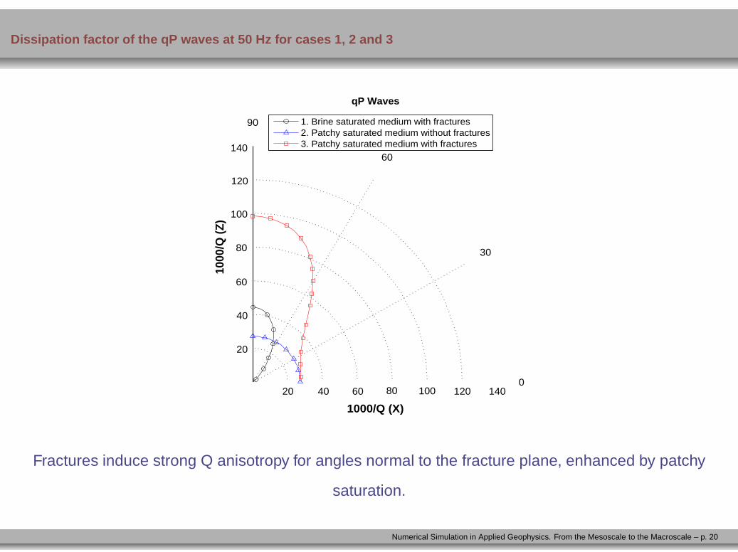
Dissipation factor of the qP waves at 50 Hz for cases 1, 2 and 3

20

40

60

80

100

120

140

30

60

90

0

qP Waves

1000/Q (X)

1000

/Q (Z

)


10080604020 120 140

Fractures induce strong Q anisotropy for angles normal to the fracture plane, enhanced by patchy

saturation.


Fluid pressure distribution at 50 and 300 Hz. Compressibili ty test for p33 for case 3.

20

40

60

80

100

120

140

160

20 40 60 80 100 120 140 160

Z (cm)

X (cm)

’Salida_presion_p33’

0

0.05

0.1

0.15

0.2

0.25

0.3

0.35

0.4

0.45

0.5

Pf (Pa)

20

40

60

80

100

120

140

160

20 40 60 80 100 120 140 160

Z (cm)

X (cm)

’Salida_presion_p33’

0

0.1

0.2

0.3

0.4

0.5

0.6

0.7

Pf (Pa)

Compression is normal to the fracture plane. Attenuation isstronger at 300 Hz.


Polar representation of the qSV energy velocity vector at 50 Hz for cases 1, 2 and 3

1.0

2.0

3.0

4.0

30

60

90

0

qSV Waves

Vex (km/s)

Vez

(km

/s)


1.0 2.0 3.0 4.0

Velocity anisotropy is induced by fractures (cases 1 and 3 ). Patchy saturation does not affect the

anisotropic behavior of the qSV velocities. Case 2 shows isotropic velocity, with higher velocity

values than for the fractured cases


Dissipation factor of qSV waves at 50 Hz for cases 1, 2 and 3

20

40

60

80

30

60

90

0

qSV Waves

1000/Q (X)

1000

/Q (Z

)


60 8020 40

qSV anisotropy is strong for angles between 30 and 60 degrees. The lossless case 2 is

represented by a triangle at the origin


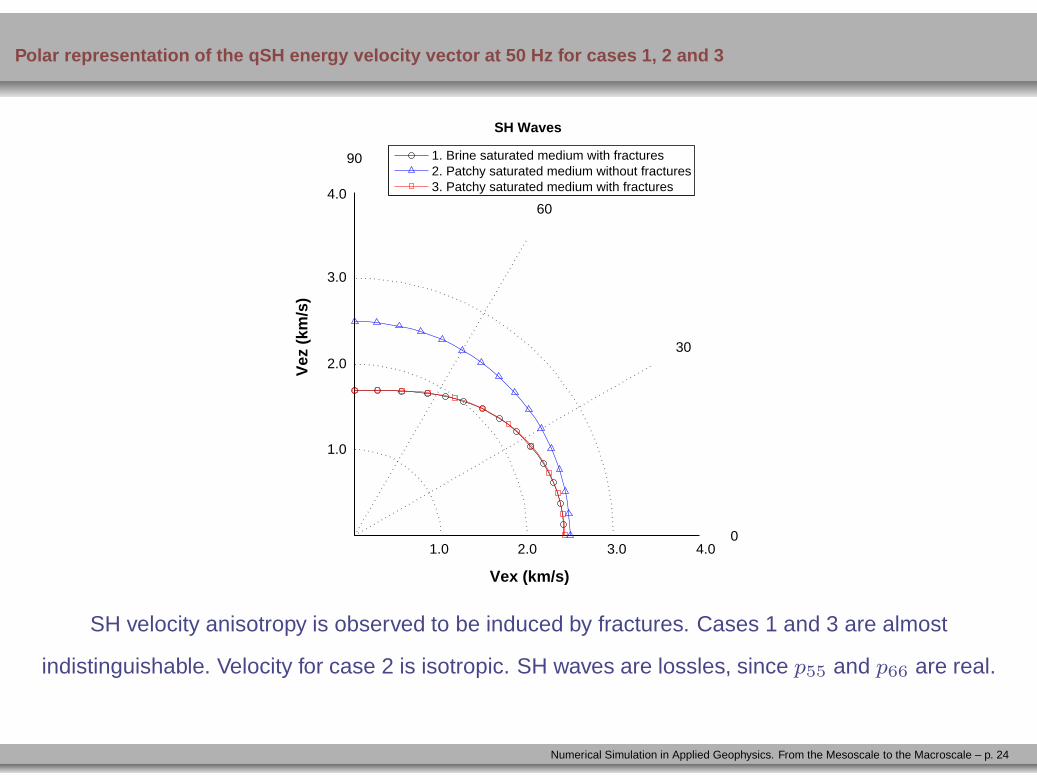
Polar representation of the qSH energy velocity vector at 50 Hz for cases 1, 2 and 3

1.0

2.0

3.0

4.0

30

60

90

0

SH Waves

Vex (km/s)

Vez

(km

/s)


1.0 2.0 3.0 4.0

SH velocity anisotropy is observed to be induced by fractures. Cases 1 and 3 are almost

indistinguishable. Velocity for case 2 is isotropic. SH waves are lossles, since p55 and p66 are real.


Lame coefficient (GPa) for the brine-saturated fractal porosit y-permeability sample of case 4.

20

40

60

80

100

120

140

160

20 40 60 80 100 120 140 160

Z (cm)

X (cm)

’lambda_global_gnu_2.dat’

3.5

4

4.5

5

5.5

6

6.5

7

λ G (GPa)

log κ(x, z) = 〈log κ〉+ f(x, z), f(x, z): fractal representing the spatial fluctuation of the

permeability field κ(x, z).


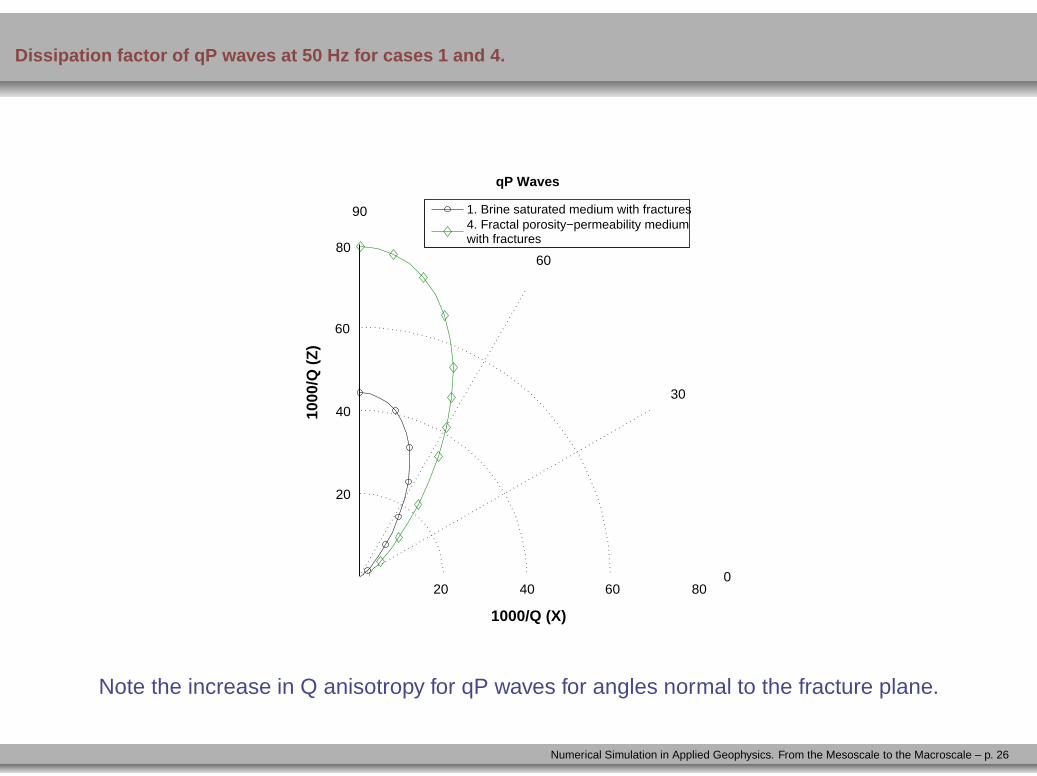
Dissipation factor of qP waves at 50 Hz for cases 1 and 4.

20

40

60

80

30

60

90

0

qP Waves

1000/Q (X)

1000

/Q (

Z)

1. Brine saturated medium with fractures4. Fractal porosity−permeability mediumwith fractures

20 60 8040

Note the increase in Q anisotropy for qP waves for angles normal to the fracture plane.


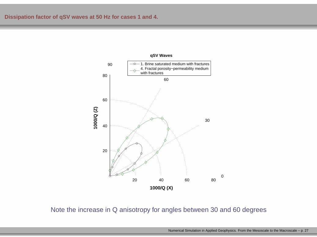
Dissipation factor of qSV waves at 50 Hz for cases 1 and 4.

20

40

60

80

30

60

90

0

qSV Waves

1000/Q (X)

1000

/Q (

Z)

1. Brine saturated medium with fractures 4. Fractal porosity−permeability mediumwith fractures

20 60 8040

Note the increase in Q anisotropy for angles between 30 and 60 degrees


The Macroscale. I

The model: Ω consists of an anisotropic rotated TIV layer between two

isotropic half-spaces.

The upper half space has P- and S-wave velocities equal to 189 0 m/s and

592 m/s, respectively, while the lower half-space has P- and S-wave

velocities of 2320 m/s and 730 m/s.

The anisotropic layer, with a thickness of 300 m, is an viscoe lastic

medium with five complex and frequency dependent stiffness o btained

using the upscaling procedure. The medium is rotated by 20 de grees , i.e.,

the angle between the symmetry axis and the vertical directi on.

The average density in Ω is 2300 kg/m3.

The mesh consists of square cells having side length 3.7 m.

The source is a dilatational perturbation of central freque ncy is 30 Hz,

located 150 m below the first interface (an asterisk in the figu res).


The Macroscale. II.

*

0 1000 m

1000 m

800 m

500 m

Source

Well 500 m

The Macroscopic TIV model.


The Macroscale. III. Seismic modeling.

We solve the following boundary value problem at the macrosc ale (in Ω):

−ω2ρu−∇ · τ(u) = F, Ω

−τ(u)ν = iωDu, ∂Ω, (absorbing bounday condition, D > 0)

u = (ux, uz): displacement vector, ρ: average density.

τ(u): stress-tensor of our equivalent viscoelastic material , defined in

terms of the p′IJs.

Instead of solving the global problem associated with the ab ove model,

we obtained the solution using a parallel FE iterative hybri dized domain

decomposition procedure employing a nonconforming FE spac e.

A run in santalo under MPI with 100 processors required 10 hou rs of CPU

time for 1000x1000 mesh, 6.000.000 unknowns and 900 frequen cies.Numerical Simulation in Applied Geophysics. From the Mesoscale to the Macroscale – p. 30

The Macroscale. IV. Snapshots of the vertical displacement at 200 ms (a and c) and 500 ms (b and d ).

*

S

S

S

S

S

SR

R

T

T

P

P

PRPT

R2

R2

P

P

T

T

*

P

P

P

T

T

SP

PR

R *

PS

PS

T

T

PR2 TP

S

SPT

SPT

PT

SPR

*

P

P

PP

P

T

T

RR

S

S

SR

R

T

A A

A A

(a)

(d)

(b)

(c)

Distance (m)

Dis

tanc

e (m

)

0

0

0

0

500

500

500

500

500 500

500 500

800

800 800

800

1000 1000

1000 1000

Ideal isotropic case (left, a and b) and real (rotated TIV) case (right, c and d).


The Macroscale. IV. CO2 injection and seismic monitoring.

Storage of CO2 in geological formations is a procedureemployed to reduce the amount of greenhouse gases in theatmosphere to slow down global warming.

Geologic sequestration involves injecting CO2 into a targetgeologic formation at depths typically >1000 m wherepressure and temperature are above the critical point for CO2

(31.6C, 7.38 MPa).

Example of injection into the Utsira Sand, a saline aquifer atthe Sleipner field, North Sea.

Time-lapse seismic surveys aim to monitor the migration anddispersal of the CO2 plume after injection.


The Macroscale. V. Permeability map (Darcy units) of the formation.

800

900

1000

1100

1200

0 300 600 900 1200

0

1

2

3

4

5

6

7

8

The thin lines represent mudstone layers within the formation.


The Macroscale. VI. Injection Modeling. Black-Oil simulator.

1200

1100

1000

900

800

0 300 600 900 1200

0

0.1

0.2

0.3

0.4

0.5

0.6

0.7

0.8

1200

1100

1000

900

800

0 300 600 900 1200

0

0.1

0.2

0.3

0.4

0.5

0.6

0.7

0.8

CO2 saturation distribution after 2 years (left) and 6 years(right) of CO2 injection


The Macroscale. VII. P-wave phase velocityvp(ω)(m/s) and attenuation coefficientQp(ω) at 50 Hz.

1200

1100

1000

900

800

0 300 600 900 1200

1000

1200

1400

1600

1800

2000

2200

2400

2600

1200

1100

1000

900

800

0 300 600 900 1200

0

20

40

60

80

100

120

140

Observe a decrease in P- wave velocity (left) and a decrease in attenuation coefficient Qp (right)

in zones of CO2 accumulation. Mesoscopic attenuation adn dispersion effects are taking into

account using a White model.


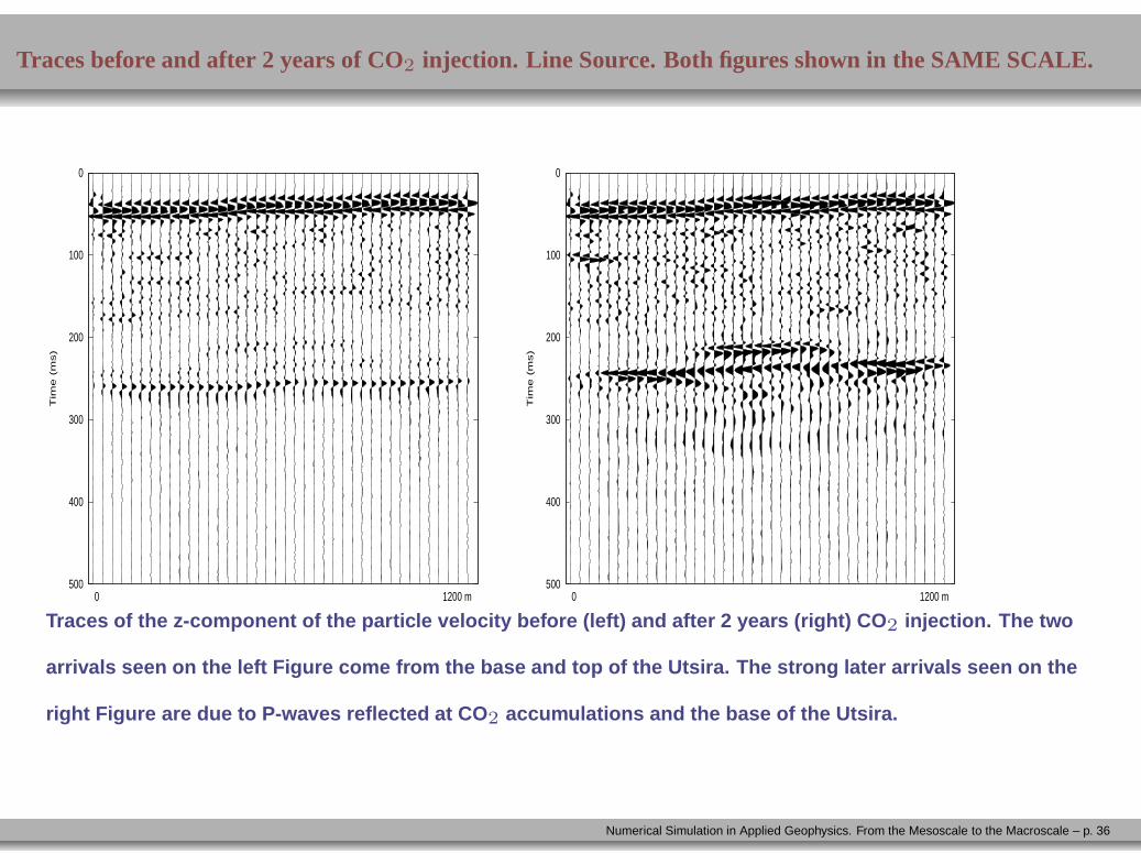
Traces before and after 2 years of CO2 injection. Line Source. Both figures shown in the SAME SCALE.

0

100

200

300

400

500

Tim

e (

ms)

0 1200 m

0

100

200

300

400

500

Tim

e (

ms)

0 1200 m

Traces of the z-component of the particle velocity before (l eft) and after 2 years (right) CO 2 injection. The two

arrivals seen on the left Figure come from the base and top of t he Utsira. The strong later arrivals seen on the

right Figure are due to P-waves reflected at CO 2 accumulations and the base of the Utsira.


Traces before and after 2 and 6 years of CO2 injection. Line Source.

0

100

200

300

400

500

Tim

e (

ms)

0 1200 m

0

100

200

300

400

500

Tim

e (

ms)

0 1200 m

Traces of the z-component of the particle velocity after 2 ye ars (left) and 6 years (right) of CO 2 injection. The

earlier arrivals on the right Figure are due to waves reflecte d at the CO 2 accumulations below the shallow

mudstone layers.


Conclusions

Numerical upscaling procedures allow to represent mesosco pic scale

heterogeneities in the solid frame and saturant fluids, frac tures and

craks affecting observations at the macroscale.

THE FEM is a useful tool to solve local problems in the context of

Numerical Rock Physics and global problems at the macroscal e.

The techniques presented here to model acoustics of porous m edia

can be extended to other fields, like ultrasound testing of qu ality of

foods, groundwater flow and contamination among others.

Thanks for your attention !!!!!.


numerical simulation in applied geophysics. from …santos/research/lidi/lidi1.pdf · numerical...

Documents