numerical analysis of 2.5-d true-amplitude diffraction...

$: Numerical analysis of 2.5-D true-amplitude diffraction ...pangea.stanford.edu/departments/geophysics/dropbox/SWP/... · Journal of Applied Geophysics 45 2000 83–96 . Numerical analysis$
Ž .Journal of Applied Geophysics 45 2000 83–96www.elsevier.nlrlocaterjappgeo

Numerical analysis of 2.5-D true-amplitude diffractionstack migration

J.C.R. Cruz), J. Urban, G. GarabitoReceived 1 January 2000; accepted 19 May 2000

Abstract

By considering arbitrary source–receiver configurations, compressional primary reflections can be imaged into time ordepth-migrated seismic sections so that the migrated wavefield amplitudes are a measure of angle-dependent reflectioncoefficients. Several migration algorithms were proposed in the recent past based on the Born or Kirchhoff approach. All ofthem are given in form of a weighted diffraction-stack integral operator that is applied to the input seismic data. The result isa migrated seismic section where at each reflection point the source wavelet is reconstructed with an amplitude proportionalto the reflection coefficient at that point. Based on the Kirchhoff approach, we derive the weight function and the diffraction

Ž .stack integral operator for a two and one-half 2.5-D seismic model and apply it to a set of synthetic seismic data in noisyenvironment. The result shows the accuracy and stability of the 2.5-D migration method as a tool for obtaining importantinformation about the reflectivity properties of the earth’s subsurface, which is of great interest for amplitude vs. offsetŽ . Ž .angle analysis. We also present a new application of the Double Diffraction Stack DDS inversion method to determinethree important parameters along the normal ray path, i.e., the angle and point of emergence at the earth surface, and also the

Ž .radius of curvature of the hypothetical Normal Incidence Point NIP wave. q 2000 Elsevier Science B.V. All rightsreserved.

Keywords: Imaging; Ray; Migration; Inversion

1. Introduction

In the recent years, we have seen an increas-ing interest in true amplitude migration meth-ods. A major part of these works dealt with this

) Corresponding author. Centro de Geosciencas, Univer-sidade Federal do Para, CP 1611, AV. Bernardo Sayao, 01,66017-900 Belem-Para, Brazil. Fax: q55-91-211-1693.

Ž .E-mail addresses: [email protected] J.C.R. Cruz , ur-Ž . Ž [email protected] J. Urban , [email protected] G. Garabito .

topic either based on the Born approximation asŽ .given by Bleistein 1987 and Bleistein et al.

Ž .1987 , or on the ray theoretical wavefield ap-Ž .proximation as given by Hubral et al. 1991

Ž .and Schleicher et al. 1993 .This paper follows the latter alternative of

working the migration problem by using the raytheoretical approximation. We consider a geo-physical situation where the propagation veloc-ity of a point-source wave does not vary along

Ž .one of the three-dimensional 3-D Cartesiancoordinate axes, the so-called two and one-halfŽ .2.5-D model.

0926-9851r00r$ - see front matter q 2000 Elsevier Science B.V. All rights reserved.Ž .PII: S0926-9851 00 00020-3

( )J.C.R. Cruz et al.rJournal of Applied Geophysics 45 2000 83–9684

Starting from the 3-D weighted modifieddiffraction stack operator as presented by Schle-

Ž .icher et al. 1993 , we derive the appropriatemethod to perform a 2.5-D true-amplitude seis-mic migration. We find the weight function tobe applied to the amplitude of the 2.5-D seismicdata.

In summary, the paper presents a theoreticaldevelopment by which we derive an expressionfor the 2.5-D weight that is a function of rayparameters. We show examples of applicationof the true-amplitude depth migration algorithmto 2.5-D synthetic seismic data in noisy envi-ronment in order to make the numerical analysismore realistic and to verify the stability andaccuracy of the algorithm. In the final part,based on the theoretical development given by

Ž . Ž .Bleistein 1987 and Tygel et al. 1993 , weŽ .apply the Double Diffraction Stack DDS in-

version method to determine normal ray param-eters, which are the keys for a more generalinterval velocity inversion problem.

2. Review of 2.5-D ray theory

2.1. The seismic model

We use the general Cartesian coordinate sys-Ž .tem being the position vector xs x, y, z . One

of the main concerns of this paper is to applythe ray field properties to the 2.5-D seismicmodel in order to study the true-amplitude seis-mic migration method. We think of the earth asa system of isotropic layers, where each layer is

Ž .constituted by a velocity field ÕsÕ x , whosefirst derivative with respect to the second com-ponent y vanishes in all space. Each layer hassmooth surfaces as upper and lower bounds.The upper bound surface S is the earth sur-o

face. The curvature of each surface is zeroalong the second component y-axis, i.e., theseismic model has a cylindrical symmetry on

Ž .the y direction Fig. 1 . The intersection be-tween the plane of symmetry ys0 and the

Fig. 1. 2.5-D seismic model. The in-plane central andparaxial rays start at the earth surface. After reflecting atthe reflector, they reach the receiver positions.

earth surface S defines the seismic line. In theo

2.5-D seismic model, the wave velocity doesnot vary along the y direction, while the point-source seismic wave causes 3-D propagation.

At our seismic experiment carried out on S ,o

we consider only P–P primary reflections to beŽ .registered at the source–receiver pairs S, G .

We assume reproducible point sources with unitstrength and receivers with identical character-istics. Their position vectors are denoted by:

x sx j and x sx j , 1Ž . ( ) Ž .s s g g

Ž .where js j ,j is a vector of parameters on1 2

S .o

The high frequency primary reflection wave-field trajectory is then described by a ray thatstarts at the source point S on S , reaches theo

reflector S at the reflection point R, definedrŽ . Ž .by a vector x sx h , hs h ,h being ar r 1 2

vector of parameters within S , and returns tor

the earth surface at G, the ray path SRG. Byconsidering the 2.5-D case, the ray path SRG isassumed to be totally contained in the planeys0.

We introduce three local Cartesian coordinatesystems with the first two having their origins at

( )J.C.R. Cruz et al.rJournal of Applied Geophysics 45 2000 83–96 85

Žthe points S and G with components x , x ,1s 2 s. Ž .x and x , x , x , respectively. The third3s 1 g 2 g 3 g

coordinate system has its origin at the point RŽ .with components x , x , x . The axes x1r 2 r 3r 1 s

and x are tangents to the seismic line, while1 g

x and x are downward normal to the S .3s 3 g oŽ . Ž .The components x and x are defined in1r 3r

such a way that the former is tangent to thereflector S within the symmetry plane ys0,r

while the latter is upward normal to the reflec-tor. The second components x , x and x2 s 2 g 2 r

have the same direction as the y component inŽ .the general Cartesian coordinate system Fig. 1 .

2.2. Ray theory

The principal component primary reflectionof the seismic wavefield generated by a com-pressional point source located at x and regis-s

tered at x is expressed in the 3-D zero-ordergŽ .ray approximation given by Cerveny 1987 as:´

U j ,t sU W tyt j . 2Ž . Ž . Ž .Ž .o

The above cited principal component primaryreflection describes the particle displacementinto direction of the ray at the receiver point G.

Ž . Ž .In Eq. 2 , W t represents the analytic point-source wavelet, i.e., this is a complex valuedfunction whose imaginary part is the Hilberttransform of the real source wavelet, and thereal part is the wavelet itself. At the receiverposition x within the surface S , the seismicg o

trace is the superposition of the principal com-ponent primary reflections.

Ž .The reflection traveltime function tst xsatisfies the 3-D eikonal equation

=tP=ts1rÕ2 x , 3Ž . Ž .

Ž .Being ÕsÕ x the P wave velocity. The am-plitude factor U can be expressed by:o

U sU Õ=t , 4Ž .o o

Ž .where U sU x is a scalar function that satis-o o

fies the 3-D transport equation, in constant den-sity and varying velocity media, given by:

2 =tP=U Õ2 x qÕ2U =2tqU =tP=Õ2Ž . Ž . Ž .o o o

s0. 5Ž .By considering only the 2.5-D wave propaga-

tion within the symmetry plane ys0, that is ofinterest, we assume j sh s0, j sj and2 2 1

h sh, simplifying the notation, so that we1Ž . Ž . Ž .have x sx j , x sx j and x sx h .s s g g r r

Ž .Following Bleistein 1986 , we introduce thefundamental in-plane slowness Õector:

tps p ,q s s=t x , z , 6Ž . Ž . Ž .

Õ x , zŽ .where the two-components unitary vector t is

Ž .tangent to the in-plane ray trajectory. In Eq. 6 ,the components p and q are the so-called hori-zontal and vertical slowness, respectively, whichare related to each other by the expression:

12qs" yp . 7Ž .( 2Õ

By using the in-plane initial values of theŽ .slowness vector p s p ,q given as:o o o

sinb cosbo op s , q s , 8Ž .o o

Õ Õo o

where b and Õ are the start angle of the rayo o

and the velocity at the source point S, respec-tively. The in-plane ray equations are alterna-tively described by:

d xsp , 9Ž .

ds

d zsq , 10Ž .

ds

d p E 1s , 11Ž .2ds Ex Õ x , zŽ .

dt 1s , 12Ž .2ds Õ x , zŽ .

Ž .where dssÕ x, z d s.


Applying the above in-plane ray equations,Ž .and considering the initial conditions 8 , to the

Ž .fundamental solution of the transport Eq. 5 asŽ .found in Cerveny 1987 , the amplitude factor´

of the in-plane reflected wavefield is computedby:

R AA Rc cU s f . 13Ž . Ž .o 2.5 LL LL2.5 2.5

Ž .In formula 13 , R is the geometrical-opticsc

reflection coefficient at the reflection point R asŽ .presented by Bleistein 1984 . The factor AA

corresponds to the total lost energy due to thetransmission across all interfaces along thewhole ray. In general, we assume this factor tobe negligible, i.e., the transmission loss to bevery small, or to be corrected by other means.The amplitude factor LL is called in-plane2.5

point-source divergence factor or geometricalspreading, whose expression will be given inthe Section 2.3.

2.3. Paraxial ray approximation

The paraxial ray approximation is based onthe a priori knowledge of a ray trajectory alsoknown as the central ray, which in our example

Ž .is the ray that starts at the source S j , reachesŽ .the reflector at the reflection point R h , and

Ž .arrives at the receiver G j . Thus, a paraxialray is any ray that starts in the vicinity of S, at

XŽ X. XŽ X.the point S j , reflects at the point R h

nearby the point R, and reaches the receiverXŽ X. Ž .point G j in the vicinity of G Fig. 1 .

By applying the concept of paraxial rays,Ž .Cerveny 1987 derived the paraxial eikonal´

equation having as solution the two-point parax-ial reflection traveltime from point SX at xX ssŽ X. X X Ž X.x j to the point G at x sx j in thes g g

vicinity of points S and G, respectively. Anequivalent second-order approximation solution

Ž .was found also by Ursin 1982 and BortfeldŽ .1989 . In this paper, we use the formalism of

Ž .Schleicher et al. 1993 tailored to the in-plane

ray trajectory. The reflection traveltime is thengiven by:

t s, g st ss0, gs0 qp gyp sŽ . Ž .R R G S

1 1G 2 S 2ysN gq N s q N g .SG S G2 2

14Ž .

Ž . Ž .In Eq. 14 , the function t ss0, gs0R

denotes the traveltime along the central ray SG,while s and g are linear distances in the axesx and x , the so-called paraxial distances.1s 1 g

Ž .These distances are obtained as follows: 1 Atthe source–receiver points SX and GX, the vec-tors xX and xX are orthogonally projected ontos g

Ž .the respective axis x and x ; 2 the dis-1s 1 g

tances s and g are then defined as havingorigin at the source–receiver points S and Gwith end at the extremity of the projections ofxX and xX , respectively. On the other hand, thes g

so-called local horizontal slowness p and pS G

are obtained by two cascaded orthogonal projec-tions of the initial and final in-plane slownessvectors at source–receiver points SX and GX ontothe respective axes x and x .1s 1 g

The quantities N G and N S are second-de-S GŽ .rivatives of the traveltime function 14 with

respect to the source and receiver coordinatesevaluated at ss0 and gs0, respectively. Theother quantity N is the second-order mixed-SG

Ž .derivative of the same traveltime function 14evaluated at ssgs0.

In the next section, we will perform the2.5-D true-amplitude migration by using aproper weighted modified diffraction stack. Forthat, we define for all points of parameters j onthe earth surface, and each point M within aspecified volume of the macro-velocity model,the diffraction in-plane traveltime curve:

t j st S, M qt M ,G st qt . 15Ž . Ž . Ž . Ž .D S G

Ž .Following Schleicher et al. 1993 , we willrefer to this curve as the Huygens traÕeltime.The traveltimes t and t denote, respectively,S G

the traveltimes from the source point S to some


arbitrary point M within the model, and fromM to the receiver point G.

For obtaining the Huygens paraxial travel-time at a reflection point within S in ther

Ž . X Ž .vicinity of R at x sx h , MsR in Eq. 15 ,r rX Ž X.with position vector x sx h , we considerr rŽ .two equations of type 14 for the paraxial

traveltime from SX to RX

t s,r st ss0, rs0 yp sqp rysN rŽ . Ž . S r SR

1 1R 2 S 2q N s q N r , 16Ž .S R2 2

and from RX to GX

t r , g st rs0, gs0 yp rqp gŽ . Ž . r G

1 1G 2 R 2yrN gq N r q N g .RG R G2 2

17Ž .

Ž . Ž .In both formulas 16 and 17 , the quantity ris the linear distance between R and the extrem-ity of the orthogonal projection of xX onto ther

axis x tangent to the reflector at the point R.1r

The local horizontal slowness p is built by twor

cascaded projections of the in-plane slownessvector at x onto the x axis.r 1 r

It is necessary to point out that in general, theearth surface is not a horizontal plane, instead, itcan be even an arbitrary surface. In our case, weconsider it as a smooth surface with cylindricalgeometry with axis in direction of the y coordi-nate. Thus, s and g are paraxial distances eval-uated within tangent planes to the earth surface

Ž X .at S and G, respectively. Moreover, x x ands sŽ X . Ž X.x x are position vectors of the points S Sg g

Ž X.and G G in the general Cartesian coordinates.The same geometrical assumption is requiredfor the reflector surface, by the way the paraxialdistance r is evaluated within the tangent plane

Ž X .at the reflection point, while x x are ther rŽ X.position vectors of the points R R .

The quantities N and N are second-orderSR RG

mixed-derivatives, respectively of the travel-Ž . Ž .times 16 and 17 calculated at ssgsrs0,

while N R and N S are the second-order deriva-S RŽ .tives of the traveltime function 16 with respect

to s and r, respectively. The quantities N G andR

N R are the second-order derivatives of the trav-GŽ .eltime function 17 with respect to r and g.

Ž . Ž .Following Bleistein 1986 , Liner 1991 ,Ž . Ž .Stockwell 1995 and Hanitzsch 1997 , the ex-

pression of the geometrical spreading factor,when tailored to the 2.5-D zero-order ray ap-proximation of the seismic wavefield, is givenby:

cos a cos a s qs( (S G S GLL s2.5 (< <Õ NNs

p=exp yi k . 18Ž .

2

Ž .In the above formula 18 , we have that aS

and a are the start and emergence angles ofG

the central ray measured with respect to thenormal at S and G on the earth surface, whileÕ is the velocity at the source point S. The terms

NN in the denominator is given by the ratio:

N NSR GRNNs . 19Ž .S GN qNR R

Moreover, we have that s and s are twoS G

quantities related with each branch of the in-plane central ray SR and RG, and calculated bythe expressions:

R Gs s Õ x d s and s s Õ x d s. 20Ž . Ž . Ž .H HS G

S R

Ž .The exponential term in Eq. 18 representsthe phase shift due to the caustics along eachbranch of the central ray. For obtaining thisfactor, it is necessary to use dynamic ray trac-ing.

Ž .From Eq. 18 , the 2.5-D geometrical spread-ing LL can be expressed then as function of2.5

the 2-D spreading LL , given by:2

LL sLL FF , FF s s qs , 21( Ž .2.5 2 2.5 2.5 S G

where FF is called the out-of-plane factor.2.5

Essentially, the LL depends only on parame-2.5


ters of 2-D rays. The 2.5-D amplitude factor ofthe zero-order ray approximation is then rewrit-ten as:

UŽ .o 2U s . 22Ž . Ž .o 2.5 FF2.5

Ž . Ž .In the expression 22 , we have that Uo 2

denotes the in-plane 2-D wavefield amplitude.An equivalent relationship between 2-D and2.5-D amplitude factors can be found in Bleis-

Ž .tein 1986 . This means that if we know the 2-Damplitude factor, we need only to divide it bythe out-of-plane factor FF in order to obtain2.5

the 2.5-D amplitude.

3. 2.5-D ray migration theory

By following the zero-order ray approxima-tion of the 2.5-D seismic wave, we have thetrue-amplitude defined as:

U t sLL U j ,tqt sR W t .Ž . Ž . Ž . Ž .TA 2.5 o R c2.5

23Ž .

In order to build the appropriate true-ampli-tude migration operator, we start from the 3-D

Ž .integral given by Schleicher et al. 1993 :

y1˙V M ,t s dj dj w j , M UŽ . Ž .HH 1 22p A

j ,tqt j , M , 24Ž . Ž .Ž .D

Ž .where the symbol P means the first derivativeŽ .with respect to time, and w j , M is the weight

function used to stack.By assuming the paraxial distances s and g

to be linear functions of j , we can write:

ssG j and gsG j , 25Ž .S G

Ž . Ž .where G s EsrEj and G s EgrEj , whichS G

are calculated at js0. In the same way, weconsider r a linear function of h so that:

ErrsG h , where G s . 26Ž .r r

Eh

Ž .As a consequence of the above relations 25Ž .and 26 , we can express the traveltime func-

Ž . Ž .tions t st j and t st j , R . Moreover,R R D DŽ . Ž .we can define the function t j , R st j , RF D

Ž .yt j .R

By using the result obtained in the AppendixŽ .by Eq. A8 , we have the 2.5-D modified

diffraction stack integral in frequency domaingiven by the stationary phase solution:

'y ivˆ ˆV R ,v f dj w j , R U j ,vŽ . Ž . Ž .H 2.5 2.5'2p A

=exp ivt j , R . 27Ž . Ž .D

Inserting the 2.5-D zero-order approximationŽ . Ž .13 of the primary reflection into integral 27we have:

'y iv Rcˆ ˆV R ,v f dj w j , R W vŽ . Ž . Ž .H 2.5' LL2p A 2.5

=exp ivt j , R . 28Ž . Ž .F

Ž .The above integral 28 is once again calcu-lated approximately by the stationary phasemethod. At this time, we apply the stationary

Ž . Ž .)phase condition Et r Ej N s0. Thus, weF jsj

have:

w j ) , R RŽ .2.5 cˆ ˆV R ,v fW v =Ž . Ž . Y)< < LLt j , R( Ž . 2.5F

= )exp ivt j , RŽ .F

ipY

)y 1ySgn t j , R . 29Ž Ž . Ž .Ž .F4

YŽ ) . Ž 2 Ž . 2.)Where t j , R s E t j , R rEj NF F jsj

is the second-order derivative of the Taylorexpansion:

t j , R st j ) , RŽ . Ž .F F

1 2Y) )q t j , R jyj . 30Ž . Ž . Ž .F2


After some algebraic manipulations involvingŽ . Ž . Ž .the 14 , 16 and 17 , we can express the

second-order derivative term by:

2G N qG NŽ .S SR G GRY

t s . 31Ž .F S GN qNŽ .R R

3.1. Weight function

The 2.5-D weight function at an arbitrarypoint M in the macro-velocity model throughthe high frequency approximation of the diffrac-tion stack integral, for a critical point j ) withinthe migration apperture A. The weight functionis then obtained so that the stack integral isasymptotically equal to the spectrum of thetrue-amplitude migrated source wavelet multi-plied by a phase shift operator. In other words,the phase of the asymptotical result is shifted bya quantity equal to the difference between thein-plane reflection and diffraction traveltimecurves at the stationary point. Thus, we have:

ˆ ) )w xŽ . Ž .R W v exp ivt j , M : j g Ac FˆŽ .V M ,v f)½ 0 : j f A

32Ž .

By using the stationary phase approximationŽ . Ž .29 and definition 32 , the 2.5-D weight func-tion is then obtained as:

w j ) , MŽ .2.5

Y)< <sLL t j , M( Ž .2.5 F

=ip

Y)exp 1ySgn t j , M . 33Ž Ž . Ž .Ž .F4

After replacing the appropriate definition ofŽ .LL as given by Eq. 18 and including the2.5

Y Ž .evaluation of t from the expression 31 , weF

have the result:

cosa cosa( S G)w j , M sFFŽ .2.5 2.5

Õs

=G N qG NS SM G GMž /N N( SM GM

=yip

exp k qk . 34Ž .1 22

Based on the 3-D weight function found inŽ .Tygel et al. 1996 by using the so-called

Ž .Beylkin’s determinant, Martins et al. 1997Ž ) .derived a similar 2.5-D weight w j , M . ThisJ

result is related with the 2.5-D weight functiongiven in the present paper by:

yip) )w j , M sw j , M exp k qk .Ž . Ž .2.5 J 1 22

35Ž .The difference between both results can be

explained by the assumption used in Beylkin

Fig. 2. Top: Synthetic seismic data used as input in the2.5-D true-amplitude depth migration algorithm, with thesignal-to-noise ratio equal to 1:0.1. Bottom: Seismic modelused for the generating the synthetic data.


Fig. 3. 2.5-D true-amplitude depth migrated seismic data,real part, obtained after migrating the synthetic seismicdata in Fig. 1.

Ž .1985 , which does not allow for any causticsalong rays.

The above weight function is to be applied tothe amplitude of the 2.5-D seismic data, that isgenerated when we have a situation of a pointsource lined up to a set of receivers in the planej s0, by considering a seismic model where2

the velocity field does not depend on the secondcoordinate j . If the chosen point M inside the2

model coincides with a real reflection point Rand jsj ), the result of applying the difraction

Ž Ž ..stack migration operator Eq. 28 to the seis-mic data is proportional to the reflection coeffi-cient. Putting this result into the point R, wehave the so-called true-amplitude depth mi-grated reflection data. In cases of special con-figurations, we can apply the weight functionŽ . Ž .34 as follows: 1 Common-offset: G sG sG S

Ž .1 for S/G; 2 Common-shot: G s0 andSŽ .G s1 when the source point S is fixed; 3G

Fig. 4. In the cross line, we have the reflection coefficients picked from the reflector position in the migrated data. Thecontinuous line corresponds to the exact value of the reflection coefficient. In the continuous line, the gaps correspond to thereflector region where there is no illumination. In the migrated result these gaps are filled by interpolated values from themigration operator.


Common-receiver: G s1 and G s0 when theS GŽ .receiver point G is fixed; and 4 Zero-offset:

G sG s1 for S'G, and then a sa , kS G S G 1

sk and s ss . In the common-midpoint2 S G

configuration, the weight function is not ade-quate because in this case, the stationary phasesolution is not valid.

4. Application of 2.5-D true-amplitude migra-tion

The true-amplitude migration algorithm wastested on synthetic data obtained from theSEIS88 ray tracing software. The seismic modelis constituted by a layer above an arbitrary

Ž .curved reflector Fig. 2 . The interval velocityof the P–P wave in the overburden is 2.5kmrs, and 3.0 kmrs in the half-space. Theseismic data was generated into a common-shotconfiguration, with the source at xs0.1 km inthe earth surface and 177 geophones positionedbetween 0.3 and 1.4 km, being the geophoneinterval distance 6.25 m. The source pulse isrepresented by a Gabor wavelet as proposed by

Ž .Gabor 1946 , with frequency 80 Hz, while theseismic trace has the sample interval of 0.5 ms.In the seismic data a random noise with uniformdistribution was added, in which the maximumvalue is 10% of the maximum amplitude of theseismic data. The macro-velocity model and theseismogram with noise are presented in Fig. 2.The seismic data were migrated by using thetrue constant velocity model, having the targetzone 0.19FxF1.32 km; 0.3FzF0.75 km,with D xs5 m and D zs1 m. The migrated

Ž .seismic image real part is presented in Fig. 3.In Fig. 4, we have the reflection coefficients,where the continuous line corresponds to theexact values, while the crosses indicate the am-plitudes determined from the migrated section.As a consequence of the addition of noise to theinput data, the seismic migration algorithm doesnot correctly recover the original source wavelet.But even in spite of the noise, we can see thatthe obtained seismic image represents the true

reflector very well. In case of noise in the data,it is not so easy to determine where the so-calledboundary effects begin to influence the migrateddata.

5. Seismic inversion method

Based on the Born and on the ray theoreticalŽ .approximations, Bleistein 1987 and Tygel et

Ž .al. 1993 , respectively, presented a new inver-sion method, the so-called DDS, through whichit is possible to estimate several parameters onthe trajectory of a selected ray between thesource and geophone, for any arbitrary configu-ration of the seismic data. This inversion tech-nique is based on the weighted diffraction stackmigration integral, used above for determiningthe reflection coefficient. In this paper, the DDSinversion technique is used to determine three

Fig. 5. Synthetic seismic data, used as input in the DDSinversion technique. The seismic model is constituted bytwo layers above a half-space, with velocities 2500 mrsŽ . Ž .upper layer and 3000 mrs bottom layer .


parameters related to the trajectory of the nor-Ž .mal reflection ray, to be known: 1 the radius

of curvature, R , of the Normal IncidenceNIPŽ .Point NIP wave associated with the normal

Ž .ray; 2 the emergence point x of the normaloŽ .reflection ray; and 3 the emergence angle bo

of the normal reflection ray. The NIP wave, asŽ .defined by Hubral 1983 , is a hypothetical

wave that starts at the reflection point at timezero, propagates with half the medium velocityand returns to the earth surface at the two-waytime of the normal ray.

By applying the DDS inversion technique,we make use of the weighted diffraction stack

Ž .integral. Alternatively, we write V M,t sŽ .V M,t , where j is the index for specifying thej

Ž .Fig. 6. Final products of the DDS inversion technique: a coordinate of the emergence points of the normal reflection rays;Ž . Ž .b radii of curvatures of the NIP waves; c emergence angles of the normal reflection rays.


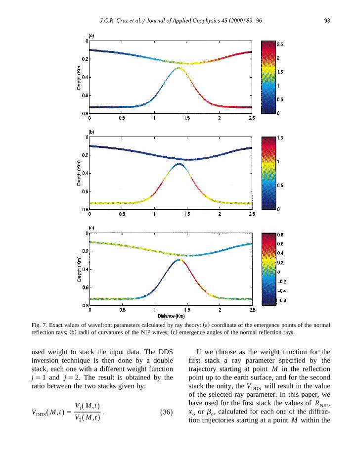
Ž .Fig. 7. Exact values of wavefront parameters calculated by ray theory: a coordinate of the emergence points of the normalŽ . Ž .reflection rays; b radii of curvatures of the NIP waves; c emergence angles of the normal reflection rays.

used weight to stack the input data. The DDSinversion technique is then done by a doublestack, each one with a different weight functionjs1 and js2. The result is obtained by theratio between the two stacks given by:

V M ,tŽ .1V M ,t s . 36Ž . Ž .DDS V M ,tŽ .2

If we choose as the weight function for thefirst stack a ray parameter specified by thetrajectory starting at point M in the reflectionpoint up to the earth surface, and for the secondstack the unity, the V will result in the valueDDS

of the selected ray parameter. In this paper, wehave used for the first stack the values of R ,NIP

x or b , calculated for each one of the diffrac-o o

tion trajectories starting at a point M within the


subsurface, having as input data a zero-offsetseismic section. The result of this inversiontechnique is a mapping of normal ray parame-ters associated with primary reflection events inthe zero-offset data. By choosing a minimumamplitude value in the denominator of the for-

Ž .mula 36 , we have empirically avoided thedivision by zero in the DDS algorithm.

6. Application of the DDS

In order to do a numerical experiment, wehave generated a set of zero-offset seismic tracesby using the ray theoretical modeling algorithmSEIS88. We have used the seismic model ofFig. 5 constituted by two layers above a half-space with two reflectors. The P–P wave ve-locities are 2500 and 3000 mrs for the firstŽ . Ž .upper and second bottom layers, respec-tively. By using a Gabor wavelet as proposed

Ž .by Gabor 1946 with a frequency of 60 Hz, asample interval of D ts1 ms and a space inter-val D xs25 m, we have obtained an ensemble

Ž .of zero-offset seismograms Fig. 5 used asinput data in the DDS process. The final prod-ucts are obtained by using the same P-wavevelocities of the original seismic model, in orderto find the following parameters of the normal

Ž .rays at the second interface: 1 the coordinatesof the emergence points of the reflection normal

Ž . Ž .rays Fig. 6a ; 2 the radii of curvaturesŽ .radiusgram of the NIP waves associated with

Ž . Ž .each reflection normal ray Fig. 6b ; and 3 theemergence angles of the reflection normal raysŽ . Ž .anglegram Fig. 6c . As we can see in Fig. 7a,b and c, the obtained values by DDS techniqueare very similar to the true values, which pro-vides an evaluation of the accuracy of the pro-posed inversion method.

In the above results, we have shown that theDDS inversion technique can be used for deter-mining a selected parameter along the ray tra-jectory. The three parameters here obtainedŽ .R , b , x are the key for solving theNIP o o

interval velocity inversion problem. A more de-

tailed discussion about the inverse problem canŽ .be found in Hubral and Krey 1980 .

7. Conclusion

Starting from the paraxial ray theory, wehave derived a 2.5-D weight function to be usedin the 2.5-D diffraction stack migration opera-tor. Based on the double diffraction stack inver-sion technique, we have also built an algorithmto determine fundamental parameters related tothe normal ray trajectory. From the results ob-tained in this paper, we claim that the present2.5-D weight function when applied to the 2.5-Dseismic data is able to recover the reflectioncoefficient even in a noisy environment. The2.5-D true-amplitude migration algorithm is sta-ble, i.e., we have that small perturbation in theinput data provides only slight deviation in theoutput migrated data. It is to be stressed that theproposed 2.5-D true-amplitude migration algo-rithm works very good in more complex situa-tions when there are triplications in the inputdata due the presence of caustics. In addition,we have shown that the DDS inversion tech-nique is able to determine parameters along theray trajectory that are of interest for the intervalvelocity inversion problem.

Acknowledgements

We thank the CNP for supporting one of theq

authors of this research, Prof. Dr. M. Tygel ofthe IMECrUNICAMPrBrazil for the fruitfuldiscussions during the preparation of this paper,and the seismic work group of the CharlesUniversity, Prague, Czech Republic, for makingthe ray tracing software SEIS88 available to us.We also thank for the important suggestions ofthree anonymous reviewers of the KarlsruheUniversity Workshop on Macro Velocity Inden-dent Seismic Imaging.


Appendix A

Ž .Following Schleicher et al. 1993 , theweighted modified diffraction stack is consid-ered an appropriate method to perform a true-amplitude migration. For each point M in the

Ž .macro-velocity model and all points j ,j in1 2

the migration aperture A, the diffraction stacksare then performed by summation along the

Ž .Huygens surfaces t j ,j , M for all points MD 1 2

into a region of the model. The true-amplitudemigration is achieved by the summation usingcertainly Huygens surface and derived weightfunction, such that the stack output is propor-tional to the desired reflection coefficient.Mathematically, this operation is described bythe 2-D integral

y1˙V M ,t s dj dj w j , M UŽ . Ž .HH 1 22p A

= j ,tqt j , M , A1Ž . Ž .Ž .D

Ž .where the symbol P means the first derivativeŽ .with respect to time, and w j , M is the weight

function used to stack.Ž .By transforming the expression A1 into the

frequency domain:

yivˆ ˆV M ,v s dj dj w j , M U jŽ . Ž . Ž .HH 1 22p A

=exp ivt j , M . A2Ž . Ž .D

Ž .In order to specialize the 3-D formula A2 tothe 2.5-D geometry, we start considering MsR, i.e., the reflection point itself. The migrationintegral needs to be solved asymptotically bythe stationary phase method as found in Bleis-

Ž .tein 1984 with respect to the coordinate j , by2

making use of the stationary condition as showedŽ .in Bleistein et al. 1987 :

Et Et S j , R Et R ,G jŽ . Ž .Ž . Ž .Ds q N s0,SoEj Ej Ej2 2 2

A3Ž .

which can be expressed through the identity:

E< <t S, M qt M ,G sp qpŽ . Ž . S S2 s 2 go oEj 2

s0. A4Ž .By applying the in-plane ray condition p s2

p into the 3-D ray equation as given by2oŽ .Cerveny 1987 , we have:´

x ss p N and x ss p N , A5Ž .2 s s 2 s S 2 g g 2 g So o

with s and s calculated along the ray pathss g

SM and MG, respectively. By considering the2.5-D geometry, x sx sj , we finally have2 s 2 g 2

the result:

1 1p qp s q j s0. A6Ž .2 s 2 g S S 2o ož /s ss g

Ž .From Eq. A6 , we conclude that the station-ary phase condition is j s0. For completeness2

of our asymptotic analysis, we calculate thesecond derivative of the phase at j s02

E2 1 1t S, R qt R ,G N s q .Ž . Ž . j s02 o o2Ej s s2 S G

A7Ž .Here, s o and s o are the ray parameters forS G

the ray branches RS and RG, calculated on theearth surface S .o

The above results yield the stationary phasesolution

'y ivV̂ R ,v f dj w j , RŽ . Ž .H'2p A

=

y1r21 1ˆq U j ,vŽ .o ož /s sS G

=exp ivt j , R , A8Ž . Ž .D

ˆŽ .As a consequence of the fact that U j ,v isthe in-plane observed point-source wavefieldamplitude factor, the 2.5-D weight function isdefined as:

y1r21 1w j , R sw j , R q , A9Ž . Ž . Ž .2.5 o ož /s sS G


Ž .where w j , R is the in-plane version of the 3-Dweight function of the 3-D modified diffraction

Ž .stack by Schleicher et al. 1993 . The weightŽ .expression A9 can be readily generalized to

any arbitrary depth point M.

References

Beylkin, G., 1985. Imaging of discontinuities in the in-verse scattering problem by inversion of a causal gener-alized radon transform. J. Math. Phys. 26, 99–108.

Bleistein, N., 1984. Mathematics of Wave Phenomena.Academic Press.

Bleistein, N., 1986. Two-and-one-half dimensional in-planewave propagation. Geophys. Prospect. 34, 686–703.

Bleistein, N., 1987. On the imaging of reflectors in theearth. Geophysics 52, 931–942.

Bleistein, N., Cohen, J.K., Hagin, F.G., 1987. Two andone-half dimensional Born inversion with an arbitraryreference. Geophysics 52, 26–36.

Bortfeld, R., 1989. Geometrical ray theory: rays and travel-Žtimes in seismic systems second-order approximation

.of the traveltimes . Geophysics 54, 342–349.Cerveny, V., 1987. Ray Methods for Three-dimensional´

Seismic Modeling. Norwegian Institute for Technology.Gabor, D., 1946. Theory of communication. J. IEEE 93,

429–441.

Hanitzsch, C., 1997. Comparison of weights in prestackamplitude-preserveing Kirchhoff depth migration. Geo-physics 62, 1812–1816.

Hubral, P., 1983. Computing true amplitude reflections inlaterally inhomogeneous earth. Geophysics 48, 1051–1062.

Hubral, P., Krey, T., 1980. Interval Velocities from Seis-mic Reflection Time Measurements. SEG.

Hubral, P., Tygel, M., Zien, H., 1991. Three-dimensionaltrue-amplitude zero-offset migration. Geophysics 56,18–26.

Liner, C., 1991. Theory of a 2.5-D acoustic wave equationfor constant density media. Geophysics 56, 2114–2117.

Martins, J.L., Schleicher, J., Tygel, M., Santos, L.T., 1997.2.5-D true-amplitude migration and demigration. J.Seism. Explor. 6, 159–180.

Schleicher, J., Tygel, M., Hubral, P., 1993. 3-D true-ampli-tude finite-offset migration. Geophysics 58, 1112–1126.

Stockwell, J.W., 1995. 2.5-D wave equations and high-frequency asymptotics. Geophysics 60, 556–562.

Tygel, M., Schleicher, J., Hubral, P., Hanitzsch, C., 1993.Multiple weights in diffraction stack migration. Geo-physics 57, 1054–1063.

Tygel, M., Schleicher, J., Hubral, P., 1996. A unifiedapproach to 3-D seismic reflection imaging: Part 2.

Ž .Theory. Geophysics 61 3 , 759–775.Ursin, B., 1982. Quadratic wavefront and traveltime ap-

proximations in inhomogeneous layered media withcurved interfaces. Geophysics 47, 1012–1021.

numerical analysis of 2.5-d true-amplitude diffraction...

Documents