numerical modelling of levee stability based on coupled mechanical

a Corresponding author: [email protected]

Numerical modelling of levee stability based on coupled mechanical, thermal and hydrogeological processes

Maciej Dwornik1,a, Krzysztof Krawiec2, Anna Franczyk1 and A�� 1 1AGH University of Science and Technology, Faculty of Geology, Geophysics and Environmental Protection, Al. Mickiewicza 30, 30-059 Krakow, Poland 2The Mineral and Energy Economy Research Institute of Polish Academy of Science, ul. Wybickiego 7, 31-261 Krakow, Poland

Abstract. The numerical modelling of coupled mechanical, thermal and hydrogeological processes for a soil levee is presented in the paper. The modelling was performed for a real levee that was built in Poland as a part of the ISMOP project. Only four parameters were changed to build different flood waves: the water level, period of water increase, period of water decrease, and period of low water level after the experiment. Results of numerical modelling shows that it is possible and advisable to calculate simultaneously changes of thermal and hydro-mechanical fields. The presented results show that it is also possible to use thermal sensors in place of more expensive pore pressure sensors, with some limitations. The results of stability analysis show that the levee is less stable when the water level decreases, after which factor of safety decreases significantly. For all flooding wave parameters described in the paper, the levee is very stable and factor of safety variations for any particular stage were not very large.

1 Introduction Levees are a popular method for protecting areas

against floods. There are over 8,000 km of levees along the main rivers in Poland [1]. The prevalence of this type of geotechnical structure makes levee monitoring a priority. Weak levees are dangerous for civil properties because they give a false impression of safety.

Nowadays, many people are looking for a universal and effective method for monitoring levee stability or predicting the time and place of their failure ([2-3]). Many projects (i.e. [4-5]) tried using thermal measurements (i.e. by using the properties of optical fibres to measure levee temperature) or other types of measurements to estimate fluid flow in levees. The aim of the ISMOP project (taken from the Polish title: Computer System for Monitoring River Embankments) is to create a complex threat forecasting system based on temperature and pore pressure sensors. To achieve this goal, an artificial full-size levee was constructed from materials commonly used for their construction.

Real measurements were preceded by numerical modelling for the mechanical, hydromechanical and thermal processes that occur during water level changes inside a water reservoir. In this paper, results of numerical modelling of the interactions between mechanical, hydromechanical and thermal processes are presented. These coupled numerical modellings were carried out in order to examine the influence of the flood wave process on the value of basic parameters that describe the state of the embankment.

2 Object of the study ��

�� !�"��#��$%&'�� ()*� �� )*� �� +')�� ,� �� ,'-.( '� /� �� 0� ��,��,� �� '��

1��,� �� 0� ��,��,��,� ��2��,�� 0�� 3�� '� �� 0��4��,��'��,�� ,�� 5� �� -2(4�� -2(')� �� -2('� �� 0�� '�� .� �� !.6� �� (7�� ,'�

DOI: 10.1051/03021 (2016), 6E3S Web of Conferences e3sconf/201

FLOODrisk 2016 - 3rd European Conference on Flood Risk Management 7 0703021

© The Authors, published by EDP Sciences. This is an open access article distributed under the terms of the Creative Commons Attribution License 4.0 (http://creativecommons.org/licenses/by/4.0/).

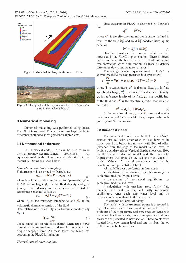
Figure 1. Model of geology medium with levee

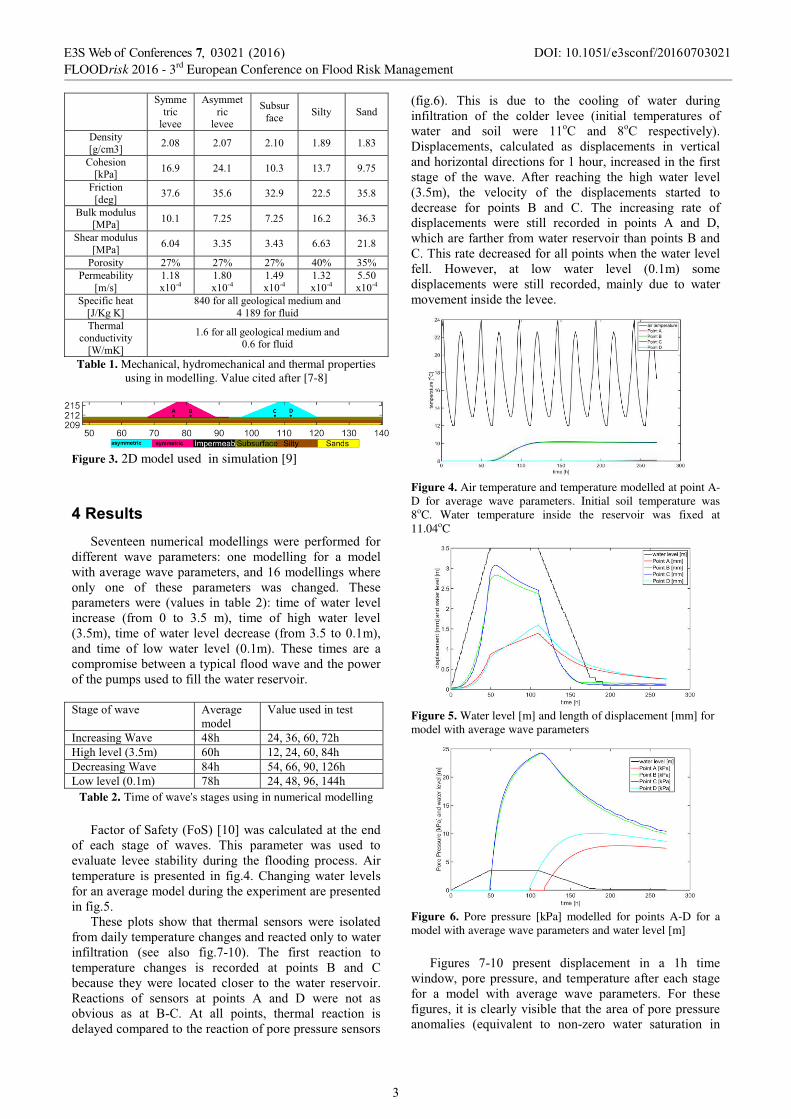
Figure 2. Photography of the experimental levee in Czernichów

near Krakow (South Poland) �

3 Numerical modeling 8�� ,� �� ,� 9��

:�� (7� ;'*� ��'� �� 0� �� ,�� '��

3.1 Mathematical background

The numerical code FLAC can be used to solve thermal-groundwater-mechanical problems [7]. All equations used in the FLAC code are described in the manual [7]. Some are listed below. Groundwater-mechanical coupling Fluid transport is described by Darcy�� law

(1) where k is fluid mobility coefficient (or �� FLAC terminology), is the fluid density and g is gravity. Fluid density in this equation is related to temperature changes as follows

(2) where is the reference temperature and is the

volumetric thermal expansion of the fluid. The relation of permeability k to hydraulic conductivity

is

. (3)

Three forces act on the solid matrix when fluid flows through a porous medium: solid weight, buoyancy, and drag or seepage force. All these forces are taken into account in the FLAC formulation. Thermal-groundwater coupling.

Heat transport in FLAC is described by Fourier�� law

(4) where is the effective thermal conductivity defined in

terms of the fluid and solid conductivities by the equation

. (5) Heat is transferred in porous media by two processes in the FLAC implementation. There is forced convection when the heat is carried by fluid motion and free convection when fluid motion is caused by density differences due to temperature variations. The energy balance equation used in FLAC for convective-diffusive heat transport is shown below.

(6) where T is temperature, is thermal flux, is fluid

specific discharge, is volumetric heat source intensity, is a reference density of the fluid, is a specific heat

of the fluid and is the effective specific heat which is defined as

. (7) In the equation above and are solid matrix bulk density and bulk specific heat, respectively, n is porosity and S is saturation.

3.2 Numerical model

�� <(+�;*�=�� ,�� *'-�'� �� (')�� (*�� ,�� 0�� '�>�� ,�� ,�� ,�� '� >�� -'�

/��,��2�.� �� =�� 0� ��

,��,� �� 5�.� �� =��

,��,� ��5�.� �� .�� 2� ��0� ��

��4� �� 4� �� 0� �� =��'� /�� 5�

.� �� :� ��0'��

��,'?'� �� '�:��4�� '�� *'+�� -�� '�

��



2

��0��

��

/0��

��

�� 0� ��

7��0�$,@ �?&� ('*A� ('*;� ('-*� -'A<� -'A?�

��$��&� -%'<� (+'-� -*'?� -?';� <';)�

:�� $�,&� ?;'%� ?)'%� ?('<� ((')� ?)'A�

B��$C��&� -*'-� ;'()� ;'()� -%'(� ?%'?�

��$C��&� %'*+� ?'?)� ?'+?� %'%?� (-'A�

��0� (;D� (;D� (;D� +*D� ?)D��0�

$�@&�-'-A��-*.+�

-'A*��-*.+�

-'+<��-*.+�

-'?(��-*.+�

)')*��-*.+�

�� $E@�,��&�

A+*��,��,� ��+�-A<��

�� 0�

$!@��&�

-'%��,��,� ��*'%��

Table 1. Mechanical, hydromechanical and thermal properties using in modelling. Value cited after [7-8]

�

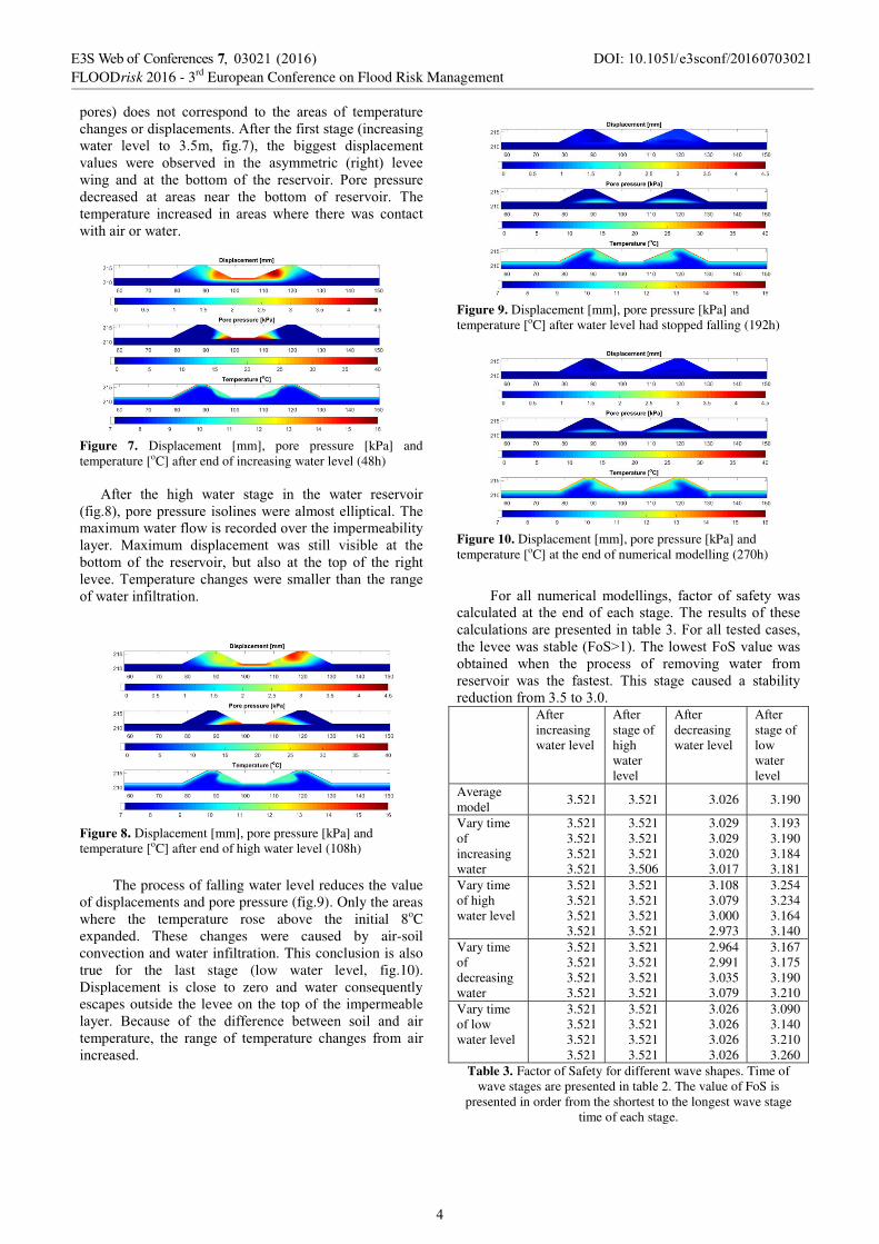
Figure 3. 2D model used in simulation [9]�

�

4 Results �� ,� ��

�� 2� �� ,� �� ,��4��-%��,��0� �� ,�'� �� ( 2� �� *� �� ?')� � 4� �� ,�� ?')� 4� �� ?')� ��*'-� 4�� *'-� '� �� 0�� '��

��,�� /��,��

��>��

9� ��,�!�� +A�� (+4�?%4�%*4�;(��F�,��?')� � %*�� -(4�(+4�%*4�A+��7� ��,�!�� A+�� )+4�%%4�<*4�-(%��G��*'-� � ;A�� (+4�+A4�<%4�-++��

Table 2. Time of wave's stages using in numerical modelling

:� ��0��:�� $-*&��

�� ,�� '� �� 0� ��,� �� ,� �� '� /�� ,'+'��,��,�� ,��,��,')'��

�� 0�� ,�� 0�� ,';.-* '� �� ,�� B� �� 0�� '�#�� /� �� 7� �� B.�'� /�� 4� �� 0��

��,'% '� �� ,� �� ,�� --�� A�� 0 '��7�� 4� �� -��4�� ,�� '� /�� ,� �� ,�� ?')� 4� �� 0� �� B� �� '� �� ,� �� /� �� 74�� B��'�� '� F��4� �� *'-� � �� 4� ��0� �� '�

Figure 4. Air temperature and temperature modelled at point A-D for average wave parameters. Initial soil temperature was 8oC. Water temperature inside the reservoir was fixed at 11.04oC

Figure 5. Water level [m] and length of displacement [mm] for model with average wave parameters

Figure 6. Pore pressure [kPa] modelled for points A-D for a model with average wave parameters and water level [m]

:�,�� ;.-*� �� -��

��4��4�� ,�� ,�� '� :�� ,��4�� 0�� =�� .��



3

�� ,�� '�/��,�� ,�� ?')�4� ��,'; 4� �� ,,�� 0�� ,�� ,� �� '� �� '� �� '�

Figure 7. Displacement [mm], pore pressure [kPa] and temperature [oC] after end of increasing water level (48h)

�/�� ,�� ,��

��,'A 4�� '�� 0��0��'� C�� 4� �� ,��'�� ,�� ,��'�

Figure 8. Displacement [mm], pore pressure [kPa] and temperature [oC] after end of high water level (108h)

The process of falling water level reduces the value

of displacements and pore pressure (fig.9). Only the areas where the temperature rose above the initial 8oC expanded. These changes were caused by air-soil convection and water infiltration. This conclusion is also true for the last stage (low water level, fig.10). Displacement is close to zero and water consequently escapes outside the levee on the top of the ��0��'� B� �� 4� �� ,�� ,�� '�

Figure 9. Displacement [mm], pore pressure [kPa] and temperature [oC] after water level had stopped falling (192h)

Figure 10. Displacement [mm], pore pressure [kPa] and temperature [oC] at the end of numerical modelling (270h)

:�� ,4� �� 0� �� ,�'� �� ?'�:�� 4��:��H- '��:�� ,� �� '� �� ,�� 0�� ?')��?'*'�� After

increasing water level

After stage of high water level

After decreasing water level

After stage of low water level

Average model

3.521 3.521 3.026 3.190

Vary time of increasing water

3.521 3.521 3.521 3.521

3.521 3.521 3.521 3.506

3.029 3.029 3.020 3.017

3.193 3.190 3.184 3.181

Vary time of high water level

3.521 3.521 3.521 3.521

3.521 3.521 3.521 3.521

3.108 3.079 3.000 2.973

3.254 3.234 3.164 3.140

Vary time of decreasing water

3.521 3.521 3.521 3.521

3.521 3.521 3.521 3.521

2.964 2.991 3.035 3.079

3.167 3.175 3.190 3.210

Vary time of low water level

3.521 3.521 3.521 3.521

3.521 3.521 3.521 3.521

3.026 3.026 3.026 3.026

3.090 3.140 3.210 3.260

Table 3. Factor of Safety for different wave shapes. Time of wave stages are presented in table 2. The value of FoS is

presented in order from the shortest to the longest wave stage time of each stage.



4

The duration of the first stage (increasing water level) had almost no effect on the FoS value after the end of the experiment (varies from 3.181 to 3.193). The biggest difference for the final FoS value was observed for high water level (varies from 3.14 to 3.25) and low water level (from 3.09 to 3.26). The long low water level duration causes levee stability to be closer to the state before the experiment.

5 Conclusions �� ,� ��

�� 0��0��.�� '�� 4� �� '�� 0� �� ,�'� 9�� 4� �� 4� ��0� �� ,0� �� ,��,��'�

/��0��0�� ,'�� 0��,�� ?')��?'*'�I�� 4��4� ��0�� :�� ,��,��0��)D '� Acknowledgements �� 0� �� 8�� #�� 7�� 8�B�# 4� ��2� ��3� ��B�-@B<@-A@(*-?��-A*)?) '�� 0� �� 0�/1F�J��0�� ,04� :� ��0� �� 1��,04�1��0� � �� 6�� 4� �� 0�� 3� �'�

6 References�

1. Borys M. (2007). Przepisy i wymogi oraz aktualny � �� Woda - ��- Obszary Wiejskie, 20(7), 25-44

2. www.urbanflood.eu 3. www.ijkdijk.eu 4. Radzicki, K. and Bonelli, S. (2012). Monitoring of

the suffusion process development using thermal analysis performed with IRFTA model, w Proc. of 6th ICSE, 593-600.

5. Bukowska-Belniak, �� !�� " �� #�� $�%�� #�� &'()*+� A 2D model of temperature changes in experimental embankment. Measurement, Automation, Monitoring, 61(6), 233-236

6. !�%��,�-��.��/��!��A. (2014). DC resistivity studies of shallow geology in the vicinity of Vistula river flood bank in Czernichów Village (near Kraków in Poland). Studia Geotechnica et Mechanica. 36 (1), 63070

7. Itasca Consulting Group, I. (2011). FLAC Fast Lagrangian Analysis of Continua and FLAC/Slope 0 1��!�5��

8. �� #�� 6�� 7�� 6�� Ptaszek, M., Stanisz, J., Korzec, K., Kret, E., 8��9��:��;��<�� !��"��M. �� =�� ,�� &'()>+�� Dokumentacja geologiczno-�� warunków geologiczno-�� projektowanej budowy eksperymentalnego ��przeciwp�� 796 w Czernichowie. AGH-UST internal documentation

9. ��!��6��6��" ��#��$�%��#��(2015) Numerical and experimental stability analysis of earthen levees. IAMG 2015: the 17th annual conference of the International Association for Mathematical Geosciences : Freiberg, Germany, Short Abstract: 163-164, Full Paper (DVD): 857-864

10. Cala, M., Flisiak, J. and 8?�5%, A. (2004). Slope stability analysis with modified shear strength reduction technique. In: Proceedings of the Ninth International � �� !"# $�� Janerio, A.A. Balkema Publishers, London, 108501089.



5

numerical modelling of levee stability based on coupled mechanical

Documents