numerical modeling of active flow control in a boundary … · 2nd aiaa flow control conference, 28...

2nd AIAA Flow Control Conference, 28 June - 1 July, 2004, Portland, Oregon

Numerical Modeling of Active Flow Control in a BoundaryLayer Ingesting Offset Inlet

Brian G. Allan∗, Lewis R. Owens†, and Bobby L. Berrier‡

NASA Langley Research Center, Hampton, VA, 23681, USA

This investigation evaluates the numerical prediction of flow distortion and pressure recovery for a bound-ary layer ingesting offset inlet with active flow control devices. The numerical simulations are computed usinga Reynolds averaged Navier-Stokes code developed at NASA. The numerical results are validated by compar-ison to experimental wind tunnel tests conducted at NASA Langley Research Center at both low and highMach numbers. Baseline comparisons showed good agreement between numerical and experimental results.Numerical simulations for the inlet with passive and active flow control also showed good agreement at lowMach numbers where experimental data has already been acquired. Numerical simulations of the inlet at highMach numbers with flow control jets showed an improvement of the flow distortion. Studies on the locationof the jet actuators, for the high Mach number case, were conducted to provide guidance for the design of afuture experimental wind tunnel test.

I. Nomenclature

AIP Aerodynamic Interface PlaneA∞ Inlet capture area, (ρ∞V∞A∞ = ρAIPVAIPAAIP)AAIP Area of inlet at AIPBL Boundary LayerBLI Boundary Layer Ingesting (or Ingestion)BWB Blended Wing BodyCFD Computational Fluid DynamicsCm jet Total jet momentum coefficient,Cm jet = (total jet momentum)/(ρ∞ U2

∞ AAIP)D AIP diameterDC60 Distortion using a 60o sectorDPCPavg Average SAE circumferential distortion descriptorL Inlet lengthM Mach numberP PressurePT Total PressurePTavg Average Total Pressure at the AIP(PTavg)crit Average Total Pressure of the ’worst’ 60◦ sectorh Vane heightMFR Mass Flow Ratio,(Total jet actuator mass flow rate)/(Inlet mass flow rate)PAVi Average total pressure of ring iPAVLOWi Average low total pressure of ring iqavg Mean dynamic pressure at the AIPReD Reynolds number based on AIP diameterD

∗Research Scientist, Flow Physics and Control Branch, NASA Langley Research Center, MS 170, Hampton, VA 23681, AIAA Senior Member.†Research Engineer, Flow Physics and Control Branch, NASA Langley Research Center, MS 170, Hampton, VA 23681, AIAA Senior Member.‡Associate Branch Head, Configuration Aerodynamics Branch, NASA Langley Research Center, MS 499, Hampton, VA 23681, and Fellow

AIAAThis material is declared a work of the U.S. Government and is not subject to copyright protection in the United States.2004

1 of 18

American Institute of Aeronautics and Astronautics Paper 2004-2318

https://ntrs.nasa.gov/search.jsp?R=20040082238 2018-07-27T07:49:14+00:00Z

sc f m Standard Cubic Feet per MinuteU∞ Free-stream Velocity,m/su,v,w Velocity in x,y,z directions respectively,m/sVG Vortex Generatorx,y,z Cartesian axesδ Boundary layer heightρ∞ Free-stream Density

A. Subscripts

avg Average∞ Free-stream

II. Introduction

IN an effort to reduce the environmental impact of commercial aircraft using revolutionary propulsion technologies,NASA initiated the Ultra Efficient Engine Technology (UEET) program.1 One of the elements of the UEET program

is the application of flush mounted, boundary layer ingesting (BLI), offset inlets on the aft portion of an aircraft.System studies for the Blended Wing Body (BWB) transport have shown significant reductions in fuel burn by usingthis type of inlet.2 For the BWB vehicle, a BLI inlet placed on the upper rear surface of the wing would have aboundary layer to inlet height ratio of 30%. The ingestion of such a large boundary layer coupled with the S-shapedoffset of the inlet diffuser, results in a large flow distortion at the engine fan face.3,4,5 Experiments have shown thatinlet distortion can be improved for the ingestion of a 30% thick boundary layer to acceptable levels using flow controldevices located inside the inlet.4

The current investigation studies the effects of vortex generating (VG) vanes and fluidic jets on inlet distortion andpressure recovery. The objectives of this investigation are twofold. The first objective is to validate the flow solverfor the BLI offset inlet flow with and without flow control by fully modeling the VG vanes and jets. Once validated,simulations of the BLI inlet, with VG jets, will be performed for a future high Mach number experiment. The resultsfrom these simulations will provide guidance on the placement of jets in the BLI inlet. The second objective of thisstudy is to provide additional insight into the flow physics of VG vanes and jets inside a BLI offset inlet. The insightsgained from the simulations of the fully modeled control devices, will be used for the future validation of a sourceterm actuator model.6 The source term model will significantly reduce the cost of simulating flow control devices inan inlet. Thus, making optimization studies for the placement and sizing of actuators in an inlet viable.

III. Numerical Modeling

Figure 1. Overset grids for VG vanes inside the BLI in-let.

The steady-state flow field for the BLI offset inlet with VGvanes and jets was computed using the flow solver code, OVER-FLOW,7,8 developed at NASA. This code solves the compressibleReynolds averaged Navier-Stokes (RANS) equations using the di-agonal scheme of Pulliam and Chaussee.9 The RANS equationsare solved on structured grids using the overset grid framework ofSteger et al.10 This overset grid framework allows for the use ofstructured grids for problems which have complex geometries. Toimprove the convergence of the steady-state solution, the OVER-FLOW code also includes a low-Mach number preconditioning op-tion and a multigrid acceleration routine, which were both used forthe numerical simulations. All of the simulations in this study usedMenter’s two-equations (k-ω) Shear-Stress Transport (SST) turbu-lence model.11 The SST turbulence model was found to be thebest turbulence model option in OVERFLOW for the simulationof streamwise vortices embedded in a boundary layer.12

The numerical simulations were performed using the parallel

2 of 18


Figure 2. Close-up view of the overset nozzle grids for a VG jetinside of the BLI inlet.

Figure 3. View of the overset nozzle grids and inlet grids.

version of the OVERFLOW code developed by Buning.13 This code uses the Message-Passing Interface (MPI) andcan run on a tightly-coupled parallel machine or a network of workstations. The code distributes zones to individualprocessors and can split larger individual zones across multiple processors using a domain decomposition approach.

The structured overset grid system was generated using the Chimera Grid Tools package.14 Figure1 shows a close-up view of the overset grids near the VG vanes on the inlet surface. The vanes were modeled as rectangular fins whichwas shown to be comparable to a fully modeled trapezoidal vane.12 Figure2 shows a close-up view of the nozzle gridsystem for the VG jet simulation. The steady jet is skewed 90o to the frees-tream flow and pitched at an inclined angleof 30o to the surface. These pitch and skew angles for the jet result in the generation of a single streamwise vortex.This jet is simulated by modeling the nozzle plenum below the surface of the inlet. This simplifies the inflow boundarycondition for the jet by letting the flow develop in the nozzle plenum and exiting at the duct surface. Figure3 showsthe inlet grids with the VG jet grids on the bottom surface of the inlet.

IV. Wind Tunnel Experiments

The numerical simulations of the BLI offset inlet were compared to two experimental tests conducted at NASALangley Research Center.3,4 One experiment was conducted in a low speed wind tunnel, the other in a high speedtransonic tunnel. The low speed experiment evaluated both passive and active flow control devices; the high speedexperiment investigated the baseline inlet at flight Mach and Reynolds numbers.

A. Low Mach and Low Reynolds Number Experiment

The low speed experiments for the BLI offset inlet were performed at NASA Langley’s Basic Aerodynamics ResearchTunnel (BART).4 This wind tunnel had a free-stream Mach number of 0.15 as was able to generate a boundary layerto inlet height ratio of 36%. The experimental test had a Reynolds number ofReD = 0.54·106, whereD = 6.0 inchesand is equal to the aerodynamic interface plane (AIP) diameter. This experiment showed the improvement of flowdistortion using VG vanes and jets located inside the inlet. The data from this experiment will be used to compare andvalidate the flow solver for low Mach number flows. Further information on the experiment is provided by Gorton etal.4

B. High Mach and High Reynolds Number Experiment

The high Mach and Reynolds number experiments were conducted at NASA Langley’s 0.3-Meter Transonic CryogenicTunnel (0.3-Meter Tunnel) for the BLI offset inlet.3 Experimental data was obtained for the baseline inlet case for a

3 of 18


free-stream Mach number range from 0.25 to 0.83. The experimental test had a Reynolds number range ofReD = 6.8·106 to 14.3 · 106, where the AIP diameter,D = 2.448 inches. This experiment was able to test the BLI inlet atactual flight Mach and Reynolds numbers as expected for the BWB aircraft application. This experiment generated aboundary layer of approximately 30% of the inlet height ratio.

C. BLI Offset Inlet Geometry

Figure 4. BLI offset inlet geometry for the 6.129% scale BART model,showing the location of flow control devices and the AIP.

The BLI offset inlet was designed by Boeing undercontract to NASA in order to provide an inlet thatwould be representative of designs considered forthe commercial version of the BWB aircraft. Theinlet geometry is of a generic nature and is an opengeometry that can be used for computational val-idation and experimental investigations. Figure4shows the side view of the S-shaped inlet for theBART experiment. The inlet for the BART experi-ment is 6.129% of full scale and the inlet model forthe 0.3-Meter Tunnel experiment was built to 2.5%scale. The inlet cross section transitions from a D-shape at the entrance to circular shape at the AIP.Figure4 also shows the location of the AIP wherethe total pressure rake was located and where theengine face would be when attached to the inlet.This figure also shows the location of the VG planewhere the passive and active flow control deviceswere placed for the BART experiment. This location has 32 jet orifices placed circumferentially on the inlet surfacewhere different combinations of jet locations were evaluated by Gorton et al.4

D. Distortion Descriptors

Two different distortion descriptors were used to evaluate inlet performance. The first inlet performance parameter isthe average SAE circumferential distortion descriptor defined in the Aerospace Recommended Practice (ARP) 1420standard. In this paper the average distortion intensity is given byDPCPavg and defined in (1).

DPCPavg =1

Nrings

Nrings

∑i=1

Intensityi (1)

wherei is the ring number on the AIP rake andNrings, the total number of rings. The Intensity for each ring is definedin (2).

Intensityi =PAVi −PAVLOWi

PAVi(2)

wherePAVi is the average total pressure of ringi andPAVLOWi , the average of the low total pressure region belowPAVi .

The second engine face distortion descriptor used isDC60 defined in (3).

DC60=PTavg− (PTavg)crit

qavg(3)

TheDC60 distortion descriptor is computed from the mean total pressure at the AIP,PTavg, the mean dynamic pressure,qavg, and the mean total pressure in the ’worst’ 60◦ sector,(PTavg)crit .15 Where the ’worst’ 60◦ sector is the sectorwith the lowest mean total pressure. Unlike theDPCPavg distortion descriptor,DC60 is scaled by the average dynamicpressure at the AIP. For experimental data,qavg is typically estimated using static pressure measurements on the surfaceof the inlet around the rake. The mean of all the static pressure measurements is then used to estimate the Mach numberat the total pressure rake locations which is then used to computeqavg. For the high Mach number cases with BLI,it was discovered using data from the numerical simulations, that this approach to estimatingqavg resulted in a 7 to

4 of 18


Figure 5. A comparison of the numerical and experimental results for the BLI inlet for the baseline low speed case, M∞ = 0.15, with a ductflow rate of 1800 scfm. These contour plots show the total pressure ratio at the AIP where the CFD results are interpolated onto the 120probe locations used in the experiment.

14% error. This estimation error inqavg is then carried over to theDC60 distortion values. For the low Mach numberexperiments, the estimation error forqavg was 1 to 4% since the static pressure did not vary as much across the AIP asin the high Mach number case. All of theDC60 results for the numerical simulations and experimental data followedthe practice of computingDC60, whereqavg is estimated from a mean static wall pressure and the total pressures at therake locations. The static and total pressures used to compute the distortion descriptors for the numerical simulationswere also interpolated at same locations as the experimental data. This way the numerical results can be evaluated atthe same resolutions as the experimental data.

V. Results and Discussions

A. Baseline: Low Mach and Low Reynolds Number Case

The baseline case for the low Mach and Reynolds number experiment had a free-stream Mach number of 0.15 with aReynolds number ofReD = 0.54·106. The duct mass flow rate was held fixed at 1800sc f mfor all low Mach numberexperimental data presented in this paper. Figure5 shows a comparison between the numerical and experimentalresults for the low Mach and Reynolds number baseline case. This figure shows the contour plots of the total pressureratio, PT/(PT)∞, at the AIP. The experimental data was taken using a 40 probe total pressure rake located at the AIP.This rake was then rotated by 15 and 30 degrees resulting in 120 total pressure measurements. The high resolution ofthe numerical results in Fig.5 are interpolated to the same resolution as the experimental data. The 120 total pressuremeasurements are then used to compute a distortion value using the DC60 method.15 The experiment had a DC60value of 0.30 where the numerical simulation was predicting 0.26. This comparison shows a difference of 13% forthe low speed baseline results. Overall the contour plots compare very well for the baseline case showing similar flowdistortion patterns.

B. Baseline: Low Mach and High Reynolds Number Case

Numerical simulations were compared to the high speed experiments taken in the 0.3-Meter Transonic CryogenicTunnel at two free-stream Mach numbers. The lower free-stream Mach cases are shown in Fig.6 whereM∞ = 0.25with mass flow rates of 6.38 and 7.10 lbm/s. These duct flow rates result in an acceleration of the flow inside the ductfor an average Mach of 0.35 at the AIP for the low mass flow rate and 0.39 for the high mass flow rate case. Thesetwo cases also have Reynolds numbers, based on the AIP diameter, of aboutReD = 6.9·106.

Since the BLI inlet was modeled on a flat plate, the effects of the tunnel walls were not accounted for in thenumerical simulations. In order to match the experimental flow conditions, the flat plate length ahead of the inlet andthe free-stream Mach number were adjusted, matching the boundary layer velocity measured near of the inlet face.The BL rake was located 3.784 inchesfrom the centerline of the inlet and 0.10 inchesupstream of the cowl highlight.The rake was approximately 1.67 inchesaway from the cowl outer surface and had a height of 0.58 inches. In the firstnumerical simulation the flat plate length was determined to match the experimental BL height. This simulation used

5 of 18


(a)

(b)

Figure 6. Comparison of numerical and experimental results for the BLI inlet for the baseline flow taken in the 0.3-Meter TransonicCryogenic Tunnel. Case(a) has a free-stream Mach of 0.25 with a ReD = 6.8 ·106 and a duct mass flow rate of 6.38 lbm/s. Case(b) has afree-stream Mach of 0.25 with a ReD = 6.9·106 and a duct mass flow rate of 7.10 lbm/s.

the free-stream Mach number given by the experiment which was measured upstream of the test section. Figure7shows the BL rake data for the high and low Mach number cases at a given inlet mass flow rate. These figures showhow the Mach number at the BL edge for the numerical simulations was slightly higher than the experiment. Thefree-stream Mach number for the simulations was then adjusted to match the velocity measured at the BL rake. Thefree-stream Mach number for theM∞ = 0.25 case was adjusted toM∞ = 0.234 in the numerical simulation, producinga better match to the BL velocity as shown in Fig.7. In the M∞ = 0.833 case, the free-stream Mach number wasreduced toM∞ = 0.784 which resulted in a better match to the BL velocity.

The BL comparison in Fig.7 shows how the BL profile is slightly different in the experiment for the high Machnumber case as compared to the numerical simulations. The BL in the experiment has less energy near the wall thanthe numerical simulation. The BL for the experiment was generated from the tunnel wall and not from a splitter plate,which may account for the difference in the BL profiles.

The flow distortion for the high Reynolds number experiments was calculated using theDPCPavg descriptor. Theflow distortion for the lower mass flow rate case had aDPCPavg = 0.005 as compared to 0.006 predicted by thenumerical simulation. The numerical simulation had a slightly lower pressure recovery ofPTavg/(PT)∞ = 0.991 whichcompares well to the experimental value of 0.994. The distortion for the higher mass flow rate was identical for thesimulation and the experiment having at value ofDPCPavg= 0.006. As in the lower mass flow rate case, the numericalresults showed a slightly lower pressure recovery of 0.989 as compared to the experiment which measured 0.994.Figure6 shows a comparison of the total pressure ratio contours which compare very well between the experimentand numerical results.

C. Baseline: High Mach and High Reynolds Number Case

The high free-stream Mach number cases are shown in Fig.8 whereM∞ = 0.833 and the duct mass flow rates were 5.0and 6.0 lbm/s. The low mass flow case had aReD = 14.3·106 and the high mass flow rate case aReD = 13.8·106. Thecomparison of distortion patterns for the high free-stream Mach number cases are good overall as seen in Fig.8. Forthe low mass flow rate case in Fig.8a, a DPCPavg of 0.040 was predicted by the numerical simulations as comparedto 0.034 measured in the experiment. The numerical simulations predict a distortion about 18% larger than was seen

6 of 18


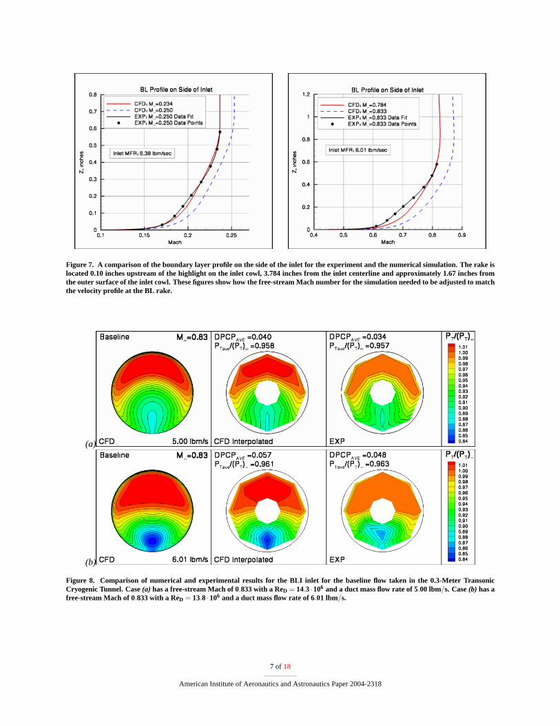
Figure 7. A comparison of the boundary layer profile on the side of the inlet for the experiment and the numerical simulation. The rake islocated 0.10 inches upstream of the highlight on the inlet cowl, 3.784 inches from the inlet centerline and approximately 1.67 inches fromthe outer surface of the inlet cowl. These figures show how the free-stream Mach number for the simulation needed to be adjusted to matchthe velocity profile at the BL rake.

(a)

(b)

Figure 8. Comparison of numerical and experimental results for the BLI inlet for the baseline flow taken in the 0.3-Meter TransonicCryogenic Tunnel. Case(a) has a free-stream Mach of 0.833 with a ReD = 14.3·106 and a duct mass flow rate of 5.00 lbm/s. Case(b) has afree-stream Mach of 0.833 with a ReD = 13.8·106 and a duct mass flow rate of 6.01 lbm/s.

7 of 18


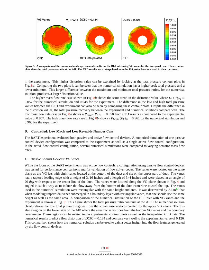
Figure 9. A comparison of the numerical and experimental results for the BLI inlet using VG vanes for the low speed case. These contourplots show the total pressure ratio at the AIP. The CFD results were interpolated onto the 120 probe locations used in the experiment.

in the experiment. This higher distortion value can be explained by looking at the total pressure contour plots inFig. 8a. Comparing the two plots it can be seen that the numerical simulation has a higher peak total pressure and alower minimum. This larger difference between the maximum and minimum total pressure ratios, for the numericalsolution, produces a larger distortion value.

The higher mass flow rate case shown in Fig.8b shows the same trend in the distortion value whereDPCPavg =0.057 for the numerical simulation and 0.048 for the experiment. The difference in the low and high total pressurevalues between the CFD and experiment can also be seen by comparing these contour plots. Despite the difference inthe distortion values, the total pressure recovery between the experiment and numerical solutions compare well. Thelow mass flow rate case in Fig.8a shows aPTavg/(PT)∞ = 0.958 from CFD results as compared to the experimentalvalue of 0.957. The high mass flow rate case in Fig.8b shows aPTavg/(PT)∞ = 0.961 for the numerical simulation and0.963 for the experiment.

D. Controlled: Low Mach and Low Reynolds Number Case

The BART experiment evaluated both passive and active flow control devices. A numerical simulation of one passivecontrol device configuration was compared to the experiment as well as a single active flow control configuration.In the active flow control configuration, several numerical simulations were compared to varying actuator mass flowrates.

1. Passive Control Devices: VG Vanes

While the focus of the BART experiments was active flow controls, a configuration using passive flow control deviceswas tested for performance comparisons and for validation of flow solver codes. The vanes were located on the sameplane as the VG jets with eight vanes located at the bottom of the duct and six on the upper part of duct. The vaneshad a tapered leading edge with a height of 3/16 inches and a length of 3/4 inches and were placed at an angle of20 degwith respect to the center line of the duct. The vanes were located along the VG plane shown in Fig.4 andangled in such a way as to induce the flow away from the bottom of the duct centerline toward the top. The vanesused in the numerical simulation were rectangular with the same height and area. It was discovered by Allan12 thatwhen modeling trapezoidal vanes submerged in a boundary layer with rectangular vanes, that one should use the sameheight as well as the same area. A comparison of the numerical simulation of the BLI inlet with VG vanes and theexperiment is shown in Fig.9. This figure shows the total pressure ratio contours at the AIP. The numerical solutionclearly shows the low total pressure regions from the streamwise vortices created by the upper VG vanes. There isalso a region on the lower side of the AIP where the streamwise vortices from the bottom VG vanes and the boundarylayer merge. These regions can be related to the experimental contour plots as well as the interpolated CFD data. Thenumerical results predict a flow distortion ofDC60= 0.134 and compare very well to the experimental value of 0.126.This comparison shows how the numerical solution can be used to gain a better insight into the flow features generatedby the flow control devices.

8 of 18


2. Active Control Devices: VG Jets

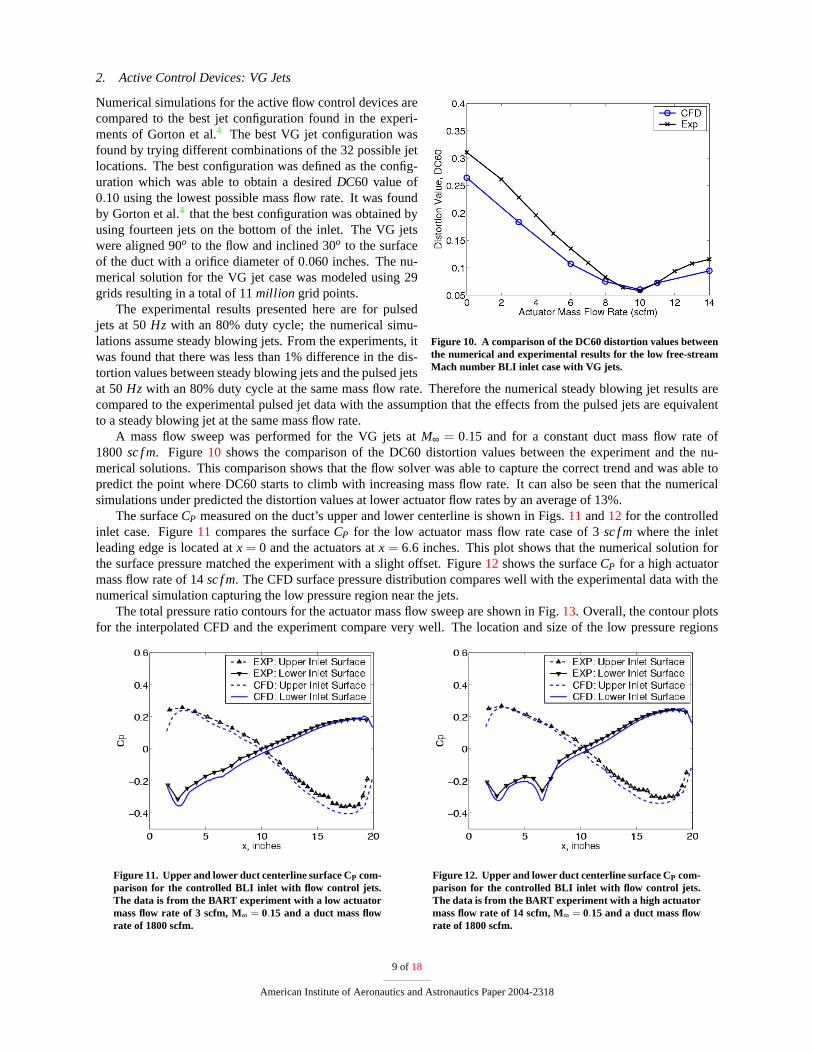
Figure 10. A comparison of the DC60 distortion values betweenthe numerical and experimental results for the low free-streamMach number BLI inlet case with VG jets.

Numerical simulations for the active flow control devices arecompared to the best jet configuration found in the experi-ments of Gorton et al.4 The best VG jet configuration wasfound by trying different combinations of the 32 possible jetlocations. The best configuration was defined as the config-uration which was able to obtain a desiredDC60 value of0.10 using the lowest possible mass flow rate. It was foundby Gorton et al.4 that the best configuration was obtained byusing fourteen jets on the bottom of the inlet. The VG jetswere aligned 90o to the flow and inclined 30o to the surfaceof the duct with a orifice diameter of 0.060 inches. The nu-merical solution for the VG jet case was modeled using 29grids resulting in a total of 11million grid points.

The experimental results presented here are for pulsedjets at 50Hz with an 80% duty cycle; the numerical simu-lations assume steady blowing jets. From the experiments, itwas found that there was less than 1% difference in the dis-tortion values between steady blowing jets and the pulsed jetsat 50Hz with an 80% duty cycle at the same mass flow rate. Therefore the numerical steady blowing jet results arecompared to the experimental pulsed jet data with the assumption that the effects from the pulsed jets are equivalentto a steady blowing jet at the same mass flow rate.

A mass flow sweep was performed for the VG jets atM∞ = 0.15 and for a constant duct mass flow rate of1800 sc f m. Figure10 shows the comparison of the DC60 distortion values between the experiment and the nu-merical solutions. This comparison shows that the flow solver was able to capture the correct trend and was able topredict the point where DC60 starts to climb with increasing mass flow rate. It can also be seen that the numericalsimulations under predicted the distortion values at lower actuator flow rates by an average of 13%.

The surfaceCP measured on the duct’s upper and lower centerline is shown in Figs.11 and12 for the controlledinlet case. Figure11 compares the surfaceCP for the low actuator mass flow rate case of 3sc f mwhere the inletleading edge is located atx = 0 and the actuators atx = 6.6 inches. This plot shows that the numerical solution forthe surface pressure matched the experiment with a slight offset. Figure12 shows the surfaceCP for a high actuatormass flow rate of 14sc f m. The CFD surface pressure distribution compares well with the experimental data with thenumerical simulation capturing the low pressure region near the jets.

The total pressure ratio contours for the actuator mass flow sweep are shown in Fig.13. Overall, the contour plotsfor the interpolated CFD and the experiment compare very well. The location and size of the low pressure regions

Figure 11. Upper and lower duct centerline surface CP com-parison for the controlled BLI inlet with flow control jets.The data is from the BART experiment with a low actuatormass flow rate of 3 scfm, M∞ = 0.15 and a duct mass flowrate of 1800 scfm.

Figure 12. Upper and lower duct centerline surface CP com-parison for the controlled BLI inlet with flow control jets.The data is from the BART experiment with a high actuatormass flow rate of 14 scfm, M∞ = 0.15 and a duct mass flowrate of 1800 scfm.

9 of 18


Figure 13. A comparison of the numerical and experimental results for the BLI offset inlet, using VG jets at various mass flows, for the lowMach number case. These contour plots show the total pressure ratio at the AIP. The CFD results were interpolated onto the 120 probelocations used in the experiment.

10 of18


Config A

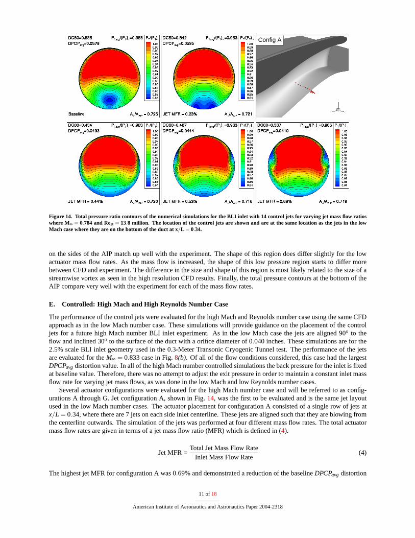
Figure 14. Total pressure ratio contours of the numerical simulations for the BLI inlet with 14 control jets for varying jet mass flow ratioswhere M∞ = 0.784 and ReD = 13.8 million. The location of the control jets are shown and are at the same location as the jets in the lowMach case where they are on the bottom of the duct at x/L = 0.34.

on the sides of the AIP match up well with the experiment. The shape of this region does differ slightly for the lowactuator mass flow rates. As the mass flow is increased, the shape of this low pressure region starts to differ morebetween CFD and experiment. The difference in the size and shape of this region is most likely related to the size of astreamwise vortex as seen in the high resolution CFD results. Finally, the total pressure contours at the bottom of theAIP compare very well with the experiment for each of the mass flow rates.

E. Controlled: High Mach and High Reynolds Number Case

The performance of the control jets were evaluated for the high Mach and Reynolds number case using the same CFDapproach as in the low Mach number case. These simulations will provide guidance on the placement of the controljets for a future high Mach number BLI inlet experiment. As in the low Mach case the jets are aligned 90o to theflow and inclined 30o to the surface of the duct with a orifice diameter of 0.040 inches. These simulations are for the2.5% scale BLI inlet geometry used in the 0.3-Meter Transonic Cryogenic Tunnel test. The performance of the jetsare evaluated for theM∞ = 0.833 case in Fig.8(b). Of all of the flow conditions considered, this case had the largestDPCPavg distortion value. In all of the high Mach number controlled simulations the back pressure for the inlet is fixedat baseline value. Therefore, there was no attempt to adjust the exit pressure in order to maintain a constant inlet massflow rate for varying jet mass flows, as was done in the low Mach and low Reynolds number cases.

Several actuator configurations were evaluated for the high Mach number case and will be referred to as config-urations A through G. Jet configuration A, shown in Fig.14, was the first to be evaluated and is the same jet layoutused in the low Mach number cases. The actuator placement for configuration A consisted of a single row of jets atx/L = 0.34, where there are 7 jets on each side inlet centerline. These jets are aligned such that they are blowing fromthe centerline outwards. The simulation of the jets was performed at four different mass flow rates. The total actuatormass flow rates are given in terms of a jet mass flow ratio (MFR) which is defined in (4).

Jet MFR =Total Jet Mass Flow Rate

Inlet Mass Flow Rate(4)

The highest jet MFR for configuration A was 0.69% and demonstrated a reduction of the baselineDPCPavg distortion

11 of18


Config B

Figure 15. Total pressure ratio contours of the numerical simulations for the BLI inlet with 14 control jets for varying jet mass flow ratioswhere M∞ = 0.784 and ReD = 13.8 million. The jets are placed near the entrance of the inlet at x/L = 0.13.

value from 0.0579 to 0.0410. TheDC60 distortion descriptor was reduced from 0.536 to 0.367. The pressure recovery,PTavg/(PT)∞, was not effected by the control jets and remained at about 0.965. The low jet MFR= 0.23% showsa spreading out of the concentrated low pressure region seen at the bottom of the AIP in the baseline case. Theintermediate jet MFR= 0.44% case shows the low pressure region smeared out along the bottom of the AIP with verylittle thinning of the ingested BL. The 0.52% jet MFR case starts showing a pooling of a low pressure region on thesides of the AIP and a slight thinning of the low pressure region. The highest MFR case of 0.69% shows larger lowpressure regions on the side of the inlet AIP with a thinning of the low pressure region on the bottom of the inlet.

Figure 16. A comparison of the area averaged total pressureratio for a 60◦ sector rotated about the AIP between the baselinecase and the controlled cases for jet configuration A and B.

Figure14 also shows the ratio of the capture area,A∞, tothe inlet AIP area,AAIP, whereA∞ is defined by (5).

A∞ ρ∞ V∞ = AAIP ρAIP VAIP (5)

The area averaged density and velocity at the AIP are givenby ρAIP andVAIP respectively. The baseline case in Fig.14hasA∞/AAIP = 0.725 which shows that the stream tube aheadof the inlet is smaller than the inlet exit area indicating a de-celeration of the flow ahead of inlet. For the high jet MFRcase, theA∞/AAIP value of 0.719 indicates a slightly lowerinlet mass flow rate than the baseline case.

Actuator configuration B is shown in Fig.15 where therow of 14 jets are moved upstream near the entrance of theinlet atx/L = 0.13. The high jet MFR case of 0.69% showsa much lowerDC60 value of 0.277 as compared to config-uration A whereDC60 = 0.367. Figure16 shows the areaaveraged 60◦ sector total pressure ratio as the sector is ro-tated about the AIP for the baseline and jet configuration Aand B cases. The ’worst’ sector average total pressure,(PTavg)crit , for all three cases is the minimum point at 180◦

which is the bottom of the AIP. This comparison of the mean sector pressures shows how the jets in configuration Bimprove the distortion at the bottom of the inlet as compared to configuration A and the baseline.

12 of18


Config C

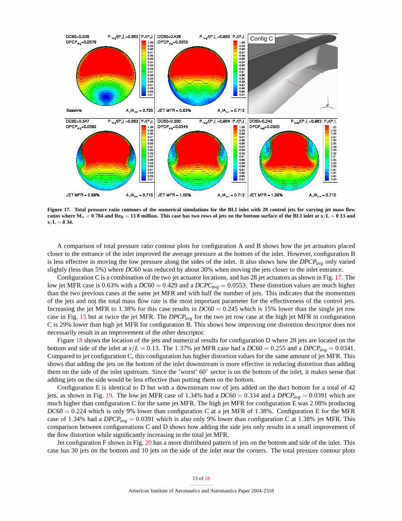
Figure 17. Total pressure ratio contours of the numerical simulations for the BLI inlet with 28 control jets for varying jet mass flowratios where M∞ = 0.784 and ReD = 13.8 million. This case has two rows of jets on the bottom surface of the BLI inlet at x/L = 0.13 andx/L = 0.34.

A comparison of total pressure ratio contour plots for configuration A and B shows how the jet actuators placedcloser to the entrance of the inlet improved the average pressure at the bottom of the inlet. However, configuration Bis less effective in moving the low pressure along the sides of the inlet. It also shows how theDPCPavg only variedslightly (less than 5%) whereDC60 was reduced by about 30% when moving the jets closer to the inlet entrance.

Configuration C is a combination of the two jet actuator locations, and has 28 jet actuators as shown in Fig.17. Thelow jet MFR case is 0.63% with aDC60= 0.429 and aDCPCavg = 0.0553. These distortion values are much higherthan the two previous cases at the same jet MFR and with half the number of jets. This indicates that the momentumof the jets and not the total mass flow rate is the most important parameter for the effectiveness of the control jets.Increasing the jet MFR to 1.38% for this case results inDC60= 0.245 which is 15% lower than the single jet rowcase in Fig.15 but at twice the jet MFR. TheDPCPavg for the two jet row case at the high jet MFR in configurationC is 29% lower than high jet MFR for configuration B. This shows how improving one distortion descriptor does notnecessarily result in an improvement of the other descriptor.

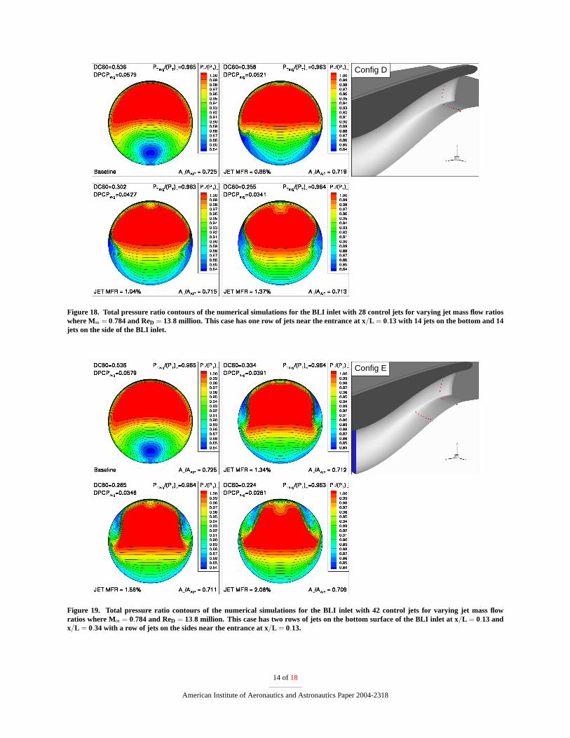
Figure18 shows the location of the jets and numerical results for configuration D where 28 jets are located on thebottom and side of the inlet atx/L = 0.13. The 1.37% jet MFR case had aDC60= 0.255 and aDPCPavg = 0.0341.Compared to jet configuration C, this configuration has higher distortion values for the same amount of jet MFR. Thisshows that adding the jets on the bottom of the inlet downstream is more effective in reducing distortion than addingthem on the side of the inlet upstream. Since the ’worst’ 60◦ sector is on the bottom of the inlet, it makes sense thatadding jets on the side would be less effective than putting them on the bottom.

Configuration E is identical to D but with a downstream row of jets added on the duct bottom for a total of 42jets, as shown in Fig.19. The low jet MFR case of 1.34% had aDC60= 0.334 and aDPCPavg = 0.0391 which aremuch higher than configuration C for the same jet MFR. The high jet MFR for configuration E was 2.08% producingDC60= 0.224 which is only 9% lower than configuration C at a jet MFR of 1.38%. Configuration E for the MFRcase of 1.34% had aDPCPavg = 0.0391 which is also only 9% lower than configuration C at 1.38% jet MFR. Thiscomparison between configureations C and D shows how adding the side jets only results in a small improvement ofthe flow distortion while significantly increasing in the total jet MFR.

Jet configuration F shown in Fig.20has a more distributed pattern of jets on the bottom and side of the inlet. Thiscase has 30 jets on the bottom and 10 jets on the side of the inlet near the corners. The total pressure contour plots

13 of18


Config D

Figure 18. Total pressure ratio contours of the numerical simulations for the BLI inlet with 28 control jets for varying jet mass flow ratioswhere M∞ = 0.784 and ReD = 13.8 million. This case has one row of jets near the entrance at x/L = 0.13 with 14 jets on the bottom and 14jets on the side of the BLI inlet.

Config E

Figure 19. Total pressure ratio contours of the numerical simulations for the BLI inlet with 42 control jets for varying jet mass flowratios where M∞ = 0.784 and ReD = 13.8 million. This case has two rows of jets on the bottom surface of the BLI inlet at x/L = 0.13 andx/L = 0.34 with a row of jets on the sides near the entrance at x/L = 0.13.

14 of18


Config F

Figure 20. Total pressure ratio contours of the numerical simulations for the BLI inlet with 40 control jets for varying jet mass flow ratioswhere M∞ = 0.784 and ReD = 13.8 million. This case has five rows of jets with each row having six jets on the bottom and two on the sideof the BLI inlet.

Config G

Figure 21. Total pressure ratio contours of the numerical simulations for the BLI inlet with 56 control jets for varying jet mass flow ratioswhere M∞ = 0.784 and ReD = 13.8 million. This case has eight rows of jets on the bottom surface of the BLI inlet with the first row having14 jets and the other rows with six jets concentrated at the center of the BLI inlet.

15 of18


Figure 22. Summary of DC60 versus the total jet MFR for all ofthe jet configurations for the high Mach and Reynolds numbercases.

Figure 23. Summary of DPCPavg versus the total jet MFR for allof the jet configurations for the high Mach and Reynolds num-ber cases.

in Fig. 20 show that this actuator pattern produces two large low pressure regions on the side of the inlet AIP. Thedistortion for the high jet MFR case shows thatDC60 is only slightly higher for the same jet MFR in configuration E.Likewise,DPCPavg is 14% higher when compared to the same jet MFR in configuration E. Jet configuration F turnsout not to perform as well as configuration E because of the higher distortion values and the larger low pressure regionson the side of the inlet.

Configuration G looked at concentrating the jets at the bottom center of the inlet where the distortion is the highest.Figure21 shows the location of the eight rows of jets for this configuration. This configuration had a total of 56 jetswhere the first row had 14 jets and the next seven rows had six jets concentrated near the bottom centerline of theinlet. The low jet MFR case was 1.82% and had aDC60 distortion of 0.226 and aDPCPavg of 0.0330. The jets onthe centerline do a good job of clearing out the center but create large low pressure regions on the side of the inlet.These regions produce the worst 60◦ sector. Increasing the jet MFR to 2.32% improves the distortion at the bottomof the AIP and moves the low pressure regions higher along the sides. The 60◦ average sector pressure for theselow pressure regions improves slightly loweringDC60 to 0.211. The 2.32% jet MFR case also reduces theDPCPavg

to 0.0302. Increasing the jet MFR to 2.87% increases the size of the low pressure regions on the side of the inletwithout changing the flow on the bottom of the AIP. This increase in the size of the low pressure regions increases thedistortion values whereDC60= 0.246% andDPCPavg = 0.0343. All three controlled cases caused a small reductionin the pressure recovery compared to the baseline case.

A plot of the distortion descriptors versus the total jet MFR for each of the jet configurations is shown in Fig.22and23. The comparison of theDC60 distortion in Fig.22 shows how none of the configurations were able to reduceDC60 below 0.2. Comparing configuration A with B indicates that moving the row of jets fromx/L = 0.34 to 0.13greatly improvedDC60 for the same number of jets at the same jet MFR. The other configurations indicate, that byadding more jets and increasing the total jet MFR, predictedDC60 can be decreased another 0.065 but at the cost oftripling the total jet MFR. The lowest predictedDC60 was 0.211 for jet configuration G with a total jet MFR of 2.32%.The best jet configuration for a jet MFR under 1% was configuration B whereDC60= 0.277 for a jet MFR= 0.69%.

Figure23shows the trend ofDPCPavg versus jet MFR for the controlled high Mach number cases. This plot showsthatDPCPavg bottoms out at 0.0281 for a jet MFR of 2% using configuration E. This figure also indicates that there islittle difference betweenDPCPavg for configurations A and B and how the combination of the two, in configuration C,continues the decreasing trend ofDPCPavg for increasing jet MFR. Figure23 also shows how the low jet MFR casesfor configuration C and D did not perform as well as A and B for a given jet MFR.

A summary of the distortion descriptors in terms of total jet momentum coefficient,Cm jet, are shown in Figs.24and 25, where the total jet momentum coefficient is defined in (6).

16 of18


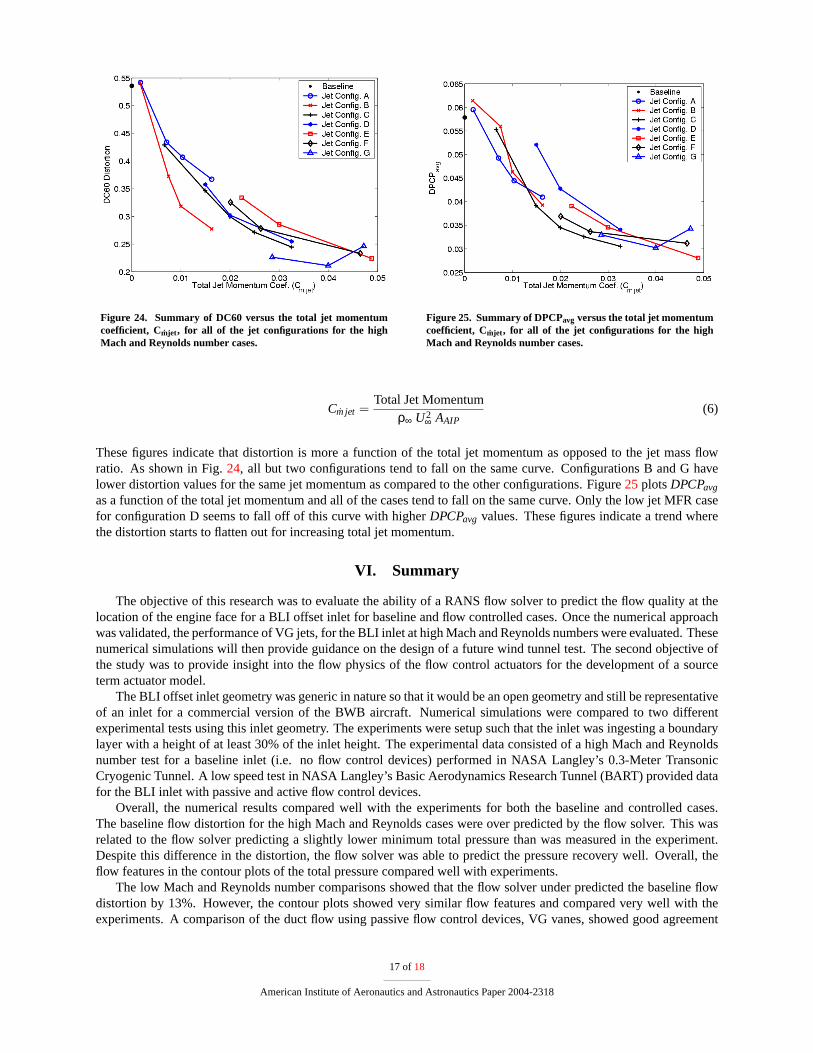
Figure 24. Summary of DC60 versus the total jet momentumcoefficient, Cmjet , for all of the jet configurations for the highMach and Reynolds number cases.

Figure 25. Summary of DPCPavg versus the total jet momentumcoefficient, Cmjet , for all of the jet configurations for the highMach and Reynolds number cases.

Cm jet =Total Jet Momentum

ρ∞ U2∞ AAIP

(6)

These figures indicate that distortion is more a function of the total jet momentum as opposed to the jet mass flowratio. As shown in Fig.24, all but two configurations tend to fall on the same curve. Configurations B and G havelower distortion values for the same jet momentum as compared to the other configurations. Figure25 plotsDPCPavg

as a function of the total jet momentum and all of the cases tend to fall on the same curve. Only the low jet MFR casefor configuration D seems to fall off of this curve with higherDPCPavg values. These figures indicate a trend wherethe distortion starts to flatten out for increasing total jet momentum.

VI. Summary

The objective of this research was to evaluate the ability of a RANS flow solver to predict the flow quality at thelocation of the engine face for a BLI offset inlet for baseline and flow controlled cases. Once the numerical approachwas validated, the performance of VG jets, for the BLI inlet at high Mach and Reynolds numbers were evaluated. Thesenumerical simulations will then provide guidance on the design of a future wind tunnel test. The second objective ofthe study was to provide insight into the flow physics of the flow control actuators for the development of a sourceterm actuator model.

The BLI offset inlet geometry was generic in nature so that it would be an open geometry and still be representativeof an inlet for a commercial version of the BWB aircraft. Numerical simulations were compared to two differentexperimental tests using this inlet geometry. The experiments were setup such that the inlet was ingesting a boundarylayer with a height of at least 30% of the inlet height. The experimental data consisted of a high Mach and Reynoldsnumber test for a baseline inlet (i.e. no flow control devices) performed in NASA Langley’s 0.3-Meter TransonicCryogenic Tunnel. A low speed test in NASA Langley’s Basic Aerodynamics Research Tunnel (BART) provided datafor the BLI inlet with passive and active flow control devices.

Overall, the numerical results compared well with the experiments for both the baseline and controlled cases.The baseline flow distortion for the high Mach and Reynolds cases were over predicted by the flow solver. This wasrelated to the flow solver predicting a slightly lower minimum total pressure than was measured in the experiment.Despite this difference in the distortion, the flow solver was able to predict the pressure recovery well. Overall, theflow features in the contour plots of the total pressure compared well with experiments.

The low Mach and Reynolds number comparisons showed that the flow solver under predicted the baseline flowdistortion by 13%. However, the contour plots showed very similar flow features and compared very well with theexperiments. A comparison of the duct flow using passive flow control devices, VG vanes, showed good agreement

17 of18


between the CFD and the low Mach number experimental data. Simulations of the VG jets were compared to anactuator mass flow sweep performed in the low Mach number experiment. This comparison indicated that the flowsolver was able to predict the inlet distortion for varying actuator mass flow. The flow solver was also able to predictthe actuator mass flow rate at the minimum distortion point.

The performance of the VG jets for the BLI inlet at high Mach and high Reynolds numbers were evaluated forseveral different actuator locations. These simulations indicated that a minimumDC60 of 0.211 could be achieved ata cost of 2.32% of the inlet mass flow. The simulations also predicted a minimumDPCPavg of 0.0281 using 2.08% ofthe inlet mass flow. From an inlet design point of view, aDC60 under 0.10 is desirable while using less than 1% of theinlet mass flow. The simulations for the high Mach number case indicate that more research needs to be performed onthe location of the actuators in order to reduce the flow distortion further. Also the simulations showed that an inletmass flow of 2% or more may be needed to acieve aDC60 value less than 0.10

The cost of fully griding the jet actuators was very high so only a few actuator patterns could be explored in thisstudy. The results from these simulations will be used to validate a source term modeling approach which will greatlyreduce the cost of modeling the jet actuators for the BLI inlet.6

VII. Acknolwegements

This research was supported by the NASA Ultra Efficient Engine Technology (UEET) Highly Integrated Inlet (HII)project. Special thanks to Ms. Susan Gorton and Mr. Scott Anders for their work and discussions on the experimentaltests and data. Also a special thanks to Dr. Pieter Buning for our discussion on the numerical flow solutions.

References1Brown, S. A., “HSR Work Propels UEET Program (High Speed Research in Ultraefficient Engine Technology in Aircraft Industry),”

Aerospace America, Vol. 37, No. 5, 1999, pp. 48–50.2Liebeck, R. H., “Design of the Blended-Wing-Body,” AIAA Paper 02–0002, January 2002.3Berrier, B. L. and Allan, B. G., “Experimental and Computational Evaluation of Flush-Mounted, S-Duct Inlets,” AIAA Paper 04–0764,

January 2004.4Gorton, S. A., Owens, L. R., Jenkins, L. N., Allan, B. G., and Schuster, E. P., “Active Flow Control on a Boundary-Layer-Ingesting Inlet,”

AIAA Paper 04–1203, January 2004.5Anabtawi, A. J., Blackwelder, R. F., Lissaman, P. B. S., and Liebeck, R. H., “An Experimental Investigation of Boundary Layer Ingestion in

a Diffusing S-Duct With and Without Passive FLow Control,” AIAA Paper 99–0739, January 2002.6Waith, K. A., “Source Term Model for Vortex Generator Vanes in a Navier-Stokes Computer Code,” AIAA Paper 2004-1236, January 2004.7Buning, P. G., Jespersen, D. C., Pulliam, T. H., Klopfer, W. M., Chan, W. M., Slotnick, J. P., Krist, S. E., and Renze, K. J., “OVERFLOW

User’s Manual Version 1.8m,” Tech. rep., NASA Langley Research Center, 1999.8Jespersen, D. C., Pulliam, T. H., and Buning, P. G., “Vortex Generator Modeling for Navier-Stokes Codes,” AIAA 97-0644, 1997.9Pulliam, T. H. and Chaussee, D. S., “A Diagonal Form of an Implicit Approximate-Factorization Algorithm,”Journal of Computational

Physics, Vol. 39, February 1981, pp. 347–363.10Steger, J. L., Dougherty, F. C., and Benek, J. A., “A Chimera Grid Scheme,”Advances in Grid Generation, edited by K. N. Ghia and U. Ghia,

Vol. 5 of FED, ASME, New York, NY, 1983.11Menter, F., “Improved Two-Equation Turbulence Models for Aerodynamic Flows,” Tech. Rep. TM 103975, NASA, NASA Langley Research

Center, Hampton, VA 23681-2199, 1992.12Allan, B. G., Yao, C. S., and Lin, J. C., “Numerical Simulations of Vortex Generator Vanes and Jets on a Flat Plate,” AIAA Paper 02–3160,

June 2002.13Murphy, K., Buning, P., Pamadi, B., Scallion, W., and Jones, K., “Status of Stage Separation Tool Development for Next Generation Launch

Technologies,” AIAA paper 04–2595, June 2004.14Chan, W. M. and Gomez, R. J., “Advances in Automatic Overset Grid Generation Around Surface Discontinuities,” AIAA Paper 99–3303,

July 1999.15Seddon, J. and Goldsmith, E. L.,Intake Aerodynamics, second Edition, AIAA, Reston, Virginia, 1999.

18 of18


numerical modeling of active flow control in a boundary … · 2nd aiaa flow control conference, 28...

Documents