Numerical method of latticeBoltzmann simulation for flowpast a rotating circular cylinder

with heat transferY.Q. Zu and Y.Y. Yan

School of the Built Environment, University of Nottingham, Nottingham, UK

W.P. ShiSchool of Mathematics, Jilin University,

Changchun, People’s Republic of China, and

L.Q. RenKey Laboratory of Terrain Machine Bionic Engineering, Jilin University,

Changchun, People’s Republic of China

Abstract

Purpose – The main objective of this work is to develop a boundary treatment in lattice Boltzmannmethod (LBM) for curved and moving boundaries and using this treatment to study numerically theflow around a rotating isothermal circular cylinder with/without heat transfer.

Design/methodology/approach – A multi-distribution function thermal LBM model is used tosimulate the flow and heat transfer around a rotating circular cylinder. To deal with the calculationson the surface of cylinder, a novel boundary treatment is developed.

Findings – The results of simulation for flow and heat transfer around a rotating cylinder includingthe evolution with time of velocity field, and the lift and drag coefficients are compared with those ofprevious theoretical, experimental and numerical studies. Excellent agreements show that presentLBM including boundary treatment can achieve accurate results of flow and heat transfer. In addition,the effects of the peripheral-to-translating-speed ratio, Reynolds number and Prandtl number onevolution of velocity and temperature fields around the cylinder are tested.

Practical implications – There is a large class of industrial processes which involve the motion offluid passing rotating isothermal circular cylinders with/without heat transfer. Operations rangingfrom paper and textile making machines to glass and plastics processes are a few examples.

Originality/value – A strategy for LBM to treat curved and moving boundary with the second-orderaccuracy for both velocity and temperature fields is presented. This kind of boundary treatment isvery easy to implement and costs less in computational time.

Keywords Fluid dynamics, Simulation, Heat transfer, Boundary layers

Paper type Research paper

The current issue and full text archive of this journal is available at

www.emeraldinsight.com/0961-5539.htm

The work is supported by the University of Nottingham’s Academic Scholarship and SiemensIndustrial Turbomachinery Ltd (UK)’s case studentship. The authors would also like to thanksfor the support from the International Collaboration Project from Chinese Scientific Ministry(Ref: 2005DFA00850) and Jilin University under the 985 programme.

HFF18,6

766

Received 21 February 2007Revised 6 September 2007Accepted 9 October 2007

International Journal of NumericalMethods for Heat & Fluid FlowVol. 18 No. 6, 2008pp. 766-782q Emerald Group Publishing Limited0961-5539DOI 10.1108/09615530810885560

Nomenclaturec ¼ streaming speed, c ; dx=dtcs ¼ velocity of soundCD ¼ drag coefficient, CD ¼ D=ðrU 2RÞCL ¼ lift coefficient, CL ¼ L=ðrU 2RÞD ¼ horizontal component of Fe ¼ discrete velocity vectorf ¼ distribution function of densityF ¼ total force acted on the solid wallg ¼ distribution function of temperatureh ¼ frequency of vortex sheddingk ¼ ratio of V to U, k ¼ V/UL ¼ vertical component of Fn ¼ outer-normal vector of cylindrical wallNu ¼ Nusselt number,

Nu ¼ 2ð2R=ðTh 2 TlÞÞð›T=›nÞwall

Pr ¼ Prandtl number, Pr ¼ n=gR ¼ radius of the circular cylinderRe ¼ Reynolds number, Re ¼ 2UR=nt ¼ timeSt ¼ Strouhal number, St ¼ hR=UT ¼ temperatureTl ¼ fluid temperature at the entranceTh ¼ temperature on the cylinder wallu ¼ velocity vectoru ¼ horizontal component of uv ¼ vertical component of uU ¼ uniform inlet velocity of the flow fieldV ¼ peripheral velocity of the cylinder

x ¼ Cartesian coordinatex ¼ horizontal component of xy ¼ vertical component of x

Greek symbolsa ¼ direction number (a ¼ 0, . . . , 8)dx ¼ time step lengthdt ¼ space step lengthf ¼ scalar arrayn ¼ kinematical viscosityr ¼ densitytn ¼ relaxation times for velocity fieldstc ¼ relaxation times for temperature fieldsv ¼ weighting coefficientg ¼ thermal diffusivityV ¼ angular velocity of the circular cylinder

Subscripts and superscriptsa ¼ direction number (a ¼ 0, . . . , 8)* ¼ dimensionless quantities, ¼ post-collision states

(eq) ¼ equilibrium states(neq) ¼ nonequilibrium partsk†l ¼ surface-averaged quantities† ¼ period-averaged quantitiesk†l ¼ period-and-surface-averaged

quantities^ ¼ approximation values

1. IntroductionThere is a large class of industrial processes which involve motion of fluid passing rotatingisothermal circular cylinders with/without heat transfer. Operations ranging from paperand textile making machines to glass and plastics processes are a few examples.

Over the past few decades, much theoretical and experimental effort has been madeto investigate isothermal flow fields past a rotating cylinder (Badr and Dennis, 1985;Bergmann et al., 2006; Coutanceau and Menard, 1985; Mittal and Kumar, 2003; Nairet al., 1998; Takada and Tsutahara, 1998). However, the studies, especially onnumerical simulations of non-isothermal flows past a rotating cylinder are still quitelimited. Therefore, the further effort is made in this paper to study numerically the flowand heat transfer from a rotating cylinder in cross-flow.

In the present study, the lattice Boltzmann method (LBM) is employed to simulatesuch flow across rotating cylinder with heat transfer. Unlike, conventional CFDsimulations which are mainly based on a direct numerical approximation to themacroscopic N-S equation, the LBM is to construct simplified kinetic models thatincorporate the essential physics of microscopic or mesoscopic processes so that themacroscopic averaged properties obey the desired macroscopic equations (Chen andDoolen, 1998). The attractive features, including the simplicity of programming, thehigh efficiency on handling interactions between the fluid and wall with complicatedgeometry, etc. make the LBM a better choice for the present simulation.

LatticeBoltzmannsimulation

767

In general, the existing LBM models for dealing with thermal fluid flows canbasically be divided into two distinct categories, namely: the multi-speed models(Alexander et al., 1993; Teixeira et al., 2000; Watari and Tsutahara, 2004) and themulti-distribution function models (Barrios et al., 2005; Guo et al., 2002a; He et al., 1998;Peng et al., 2003; Shi et al., 2004). In the multi-speed models, only the densitydistribution function is used; to obtain the macroscopic energy equation, additionaldiscrete velocities are introduced; and the equilibrium distributions usually includehigher order velocity terms. In the multi-distribution function models, in addition to theoriginal density distribution function, a distribution function for temperature is alsointroduced. This kind of models can effectively overcome two limitations of themulti-speed models, namely, severe numerical instability and narrow range oftemperature variation (He et al., 1998). Therefore, in the present study and simulation,a multi-distribution function model is chosen as the numerical scheme.

To handle the moving curved boundary of temperature field, an extrapolationmethod based on the idea of Guo et al. (2002b) will be extended. The method combinedwith the velocity boundary treatment presented by Mei et al. (2002) can satisfy thesecond-order accuracy for both velocity and temperature on the curved wall.

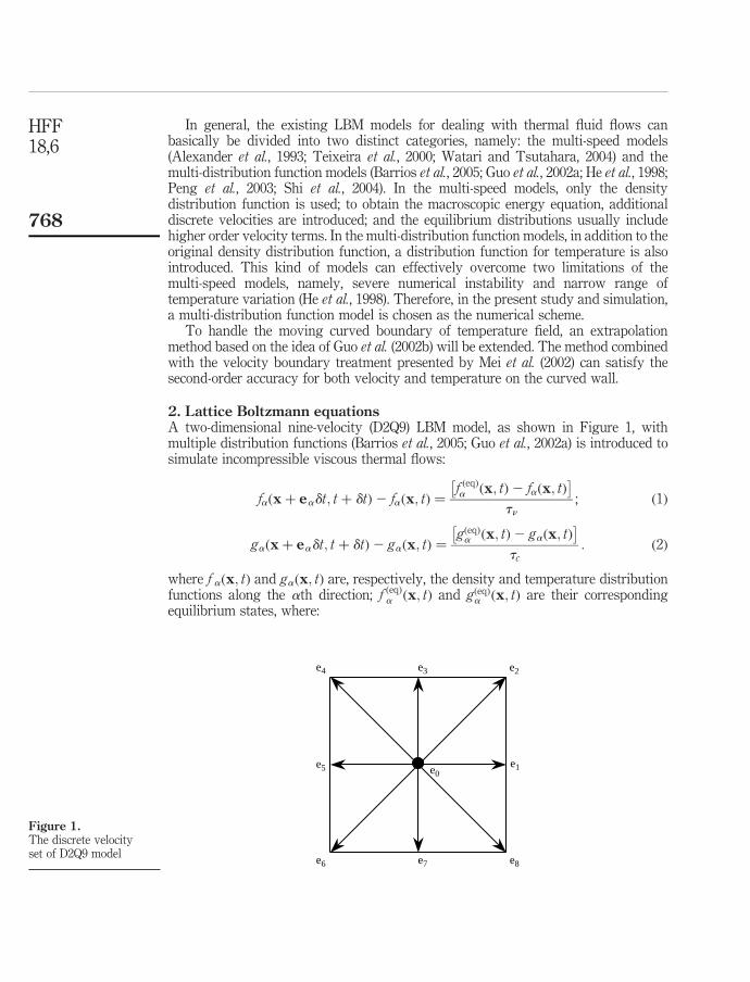
2. Lattice Boltzmann equationsA two-dimensional nine-velocity (D2Q9) LBM model, as shown in Figure 1, withmultiple distribution functions (Barrios et al., 2005; Guo et al., 2002a) is introduced tosimulate incompressible viscous thermal flows:

faðxþ eadt; t þ dtÞ2 faðx; tÞ ¼f ðeqÞa ðx; tÞ2 faðx; tÞ� �

tn; ð1Þ

gaðxþ eadt; t þ dtÞ2 gaðx; tÞ ¼gðeqÞa ðx; tÞ2 gaðx; tÞ

� �tc

: ð2Þ

where f aðx; tÞ and gaðx; tÞ are, respectively, the density and temperature distributionfunctions along the ath direction; f ðeqÞ

a ðx; tÞ and gðeqÞa ðx; tÞ are their corresponding

equilibrium states, where:

Figure 1.The discrete velocityset of D2Q9 model

e1

e2

e8e7e6

e5

e4 e3

e0

HFF18,6

768

f ðeqÞa ðx; tÞ ¼ var 1 þ

3

c 2ðea ·uÞ þ

9

2c 2ðea ·uÞ2 2

3

2c 2u2

� �; ð3Þ

gðeqÞa ðx; tÞ ¼ vaT 1 þ

3

c2ea ·u

� �; ð4Þ

ea ¼

0; a ¼ 0

ðcos½ða2 1Þp=4�; sin½ða2 1Þp=4�Þc; a ¼ 1; 3; 5; 7ffiffiffi2

pðcos½ða2 1Þp=4�; sin½ða2 1Þp=4�Þc; a ¼ 2; 4; 6; 8

;

8>><>>: ð5Þ

va ¼

4=9; a ¼ 0

1=9; a ¼ 1; 3; 5; 7

1=36; a ¼ 2; 4; 6; 8

;

8>><>>: ð6Þ

where cs ¼ c=ffiffiffi3

pis the speed of sound, other parameters such as u, r, T, n and g are

evaluated as:

r ¼a

Xf a; ru ¼

a

Xea f a; T ¼

a

Xga; n ¼

tn 2 0:5

c2sdt

; g ¼tc 2 0:5

c2sdt

: ð7Þ

Under the incompressible flow limit (i.e. the Mach number Ma ¼ juj=cs ,, 1), throughthe Chapman-Enskog expansion, the mass, momentum and energy equations can bederived from the D2Q9 model as follows (Guo et al., 2002a; Yu et al., 2003):

7 ·u ¼ 0; ð8Þ

›u

›tþ ðu ·7Þu ¼ 2

1

r7pþ n72u; ð9Þ

›T

›tþ 7 · ðuTÞ ¼ g72T: ð10Þ

3. Curved boundary treatment in LBMEquations (1) and (2) can be computed by the following two steps, i.e. collision andstreaming:

Collision step : ~faðx; tÞ ¼ f aðx; tÞ2f aðx; tÞ2 f ðeqÞ

a ðx; tÞ� �

tn; ð11aÞ

~gaðx; tÞ ¼ gaðx; tÞ2gaðx; tÞ2 gðeqÞ

a ðx; tÞ� �

tc; ð11bÞ

Streaming step : faðxþ eadt; t þ dtÞ ¼ ~faðx; tÞ; ð12aÞ

gaðxþ eadt; t þ dtÞ ¼ ~gaðx; tÞ: ð12bÞ

LatticeBoltzmannsimulation

769

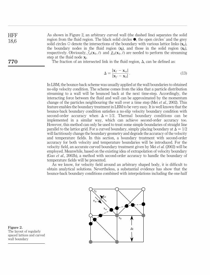
As shown in Figure 2, an arbitrary curved wall (the dashed line) separates the solidregion from the fluid region. The black solid circles X, the open circlesˆ and the greysolid circles W denote the intersections of the boundary with various lattice links (xw),the boundary nodes in the fluid region (xf), and those in the solid region (xb),respectively. Obviously, ~f �aðxb; tÞ and ~g �aðxb; tÞ are needed to perform the streamingstep at the fluid node xf.

The fraction of an intersected link in the fluid region, D, can be defined as:

D ¼jxf 2 xwj

jxf 2 xbj: ð13Þ

In LBM, the bounce-back scheme was usually applied at the wall boundaries to obtainedno-slip velocity condition. The scheme comes from the idea that a particle distributionstreaming to a wall will be bounced back at the next time-step. Accordingly, theinteracting force between the fluid and wall can be approximated by the momentumchange of the particles neighbouring the wall over a time step (Mei et al., 2002). Thisfeature enables the boundary treatment in LBM to be very easy. It is well known that thebounce-back boundary condition satisfies a no-slip velocity boundary condition withsecond-order accuracy when D ¼ 1/2. Thermal boundary conditions can beimplemented in a similar way, which can achieve second-order accuracy too.However, this method can only be used to treat some simple boundaries of straight lineparallel to the lattice grid. For a curved boundary, simply placing boundary at D ¼ 1/2will factitiously change the boundary geometry and degrade the accuracy of the velocityand temperature fields. In this section, a boundary treatment with second-orderaccuracy for both velocity and temperature boundaries will be introduced. For thevelocity field, an accurate curved boundary treatment given by Mei et al. (2002) will beemployed. Meanwhile, based on the existing idea of extrapolation of velocity boundary(Guo et al., 2002b), a method with second-order accuracy to handle the boundary oftemperature fields will be presented.

As we know, for velocity field around an arbitrary shaped body, it is difficult toobtain analytical solutions. Nevertheless, a substantial evidence has show that thebounce-back boundary conditions combined with interpolations including the one-half

Figure 2.The layout of regularlyspaced lattices and curvedwall boundary

eaea

xw

xb

xf

dx

HFF18,6

770

grid spacing correction at boundaries, are in fact of second-order accurate and thusca-pable of handling curved boundaries (Mei et al., 2002; Yu et al., 2003). ~f �aðxb; tÞ can beconstructed based upon some know information in the surrounding:

~f �aðxb; tÞ ¼ ~faðxf ; tÞ2 x ~faðxf ; tÞ2 f ðeqÞa ðxf ; tÞ

� �þ varðxf ; tÞ

3

c 2ea · ½xðubf 2 uf Þ2 2uw�;

ð14Þ

where:

ubf ¼ uff ¼ uðxff ; tÞ; x ¼2D2 1

t2 2; if 0 # D ,

1

2; ð15aÞ

ubf ¼1

2Dð2D2 3Þuf þ

3

2Duw; x ¼

2D2 1

t2 ð1=2Þ; if

1

2# D , 1: ð15bÞ

In the above:

e �a ; 2ea; xff ¼ xf þ e �adt; uf ; uðxf ; tÞ; uw ; uðxw; tÞ;

where ubf is the imaginary velocity for interpolations, and x is weight factor.To implement the curved boundary treatment for temperature, the non-equilibrium

parts of temperature distribution function, gðneqÞa ðx; tÞ ¼ gaðx; tÞ2 gðeqÞ

a ðx; tÞ, isintroduced. Let the temperature at xw, xf and xff be Tw, Tf and Tff, respectively.Then, ~g �aðxb; tÞ can be approximated by an extrapolation method with second-orderaccuracy:

~g �aðxb; tÞ ¼1 2 1

tcgðneqÞ

�a ðxb; tÞ þ v �aTb 1 þ 3e �a ·ub

c2

� �; ð16Þ

gðneqÞ�a ðxb; tÞ ¼ gðneqÞ

�a ðxf ; tÞ

ub ¼ ½uw þ ðD2 1Þuf �=D

Tb ¼ ½Tw þ ðD2 1ÞTf �=D

9>>>=>>>;; if D $ 0:75; ð17aÞ

gðneqÞ�a ðxb; tÞ ¼ DgðneqÞ

�a ðxf ; tÞ þ ð1 2 DÞgðneqÞ�a ðxff ; tÞ

ub ¼ uw þ ðD2 1Þuf þ ½2uw þ ðD2 1Þuff �ð1 2 DÞ=ð1 þ DÞ

Tb ¼ Tw þ ðD2 1ÞTf þ ½2Tw þ ðD2 1ÞTff �ð1 2 DÞ=ð1 þ DÞ

9>>>=>>>;;

if D , 0:75:

ð17bÞ

Consequently, on the temperature boundary, the second-order accuracy can besatisfied by using ~h �aðxb; tÞ to approximate ~g �aðxb; tÞ.

It should be noted that the present boundary treatment for velocity and temperaturefields inherits the basic idea of the bounce back scheme. Therefore, it is easy to beimplemented and costs less in computational time.

In the present simulation, a momentum-exchange method (Mei et al., 2002) isemployed to evaluate the force on the circular cylinder surface. In order to implement

LatticeBoltzmannsimulation

771

the method efficiently, a scalar array f(i, j) is employed. f(i, j) ¼ 0 refers to that thelattice location (i, j) is occupied by fluid; For those lattice nodes inside the solid body,f(i, j) ¼ 1 is given. For a given boundary node xb inside the solid region, themomentum-exchange with all possible neighboring fluid nodes over a time step isgiven by:

a–0

Xea½ ~faðxb; tÞ þ ~f �aðxb þ e �adt; tÞ�½1 2 fðxb þ e �adtÞ�: ð18Þ

The total force acted on the solid body by fluid can be obtained by summing thecontribution over all boundary nodes xb belonging to the body, i.e.:

F ¼all xb

XXa–0

ea½ ~faðxb; tÞ þ ~f �aðxb þ e �adt; tÞ�½1 2 fðxb þ e �adtÞ�: ð19Þ

In the momentum-exchange method, force F is evaluated after the collision step andthat the value of ~f �a on the boundary given by equation (14) is also evaluated.

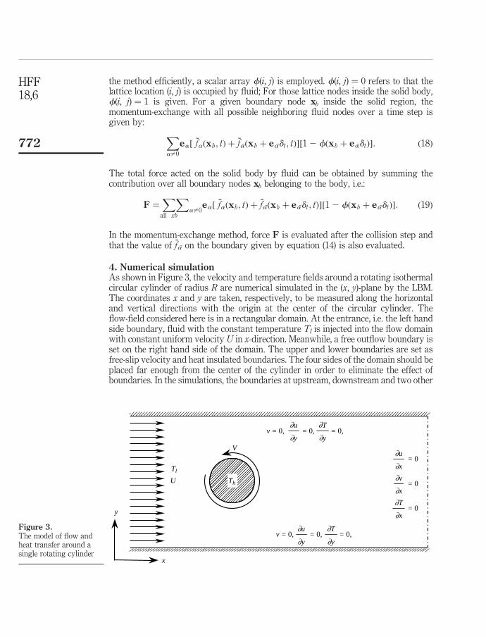
4. Numerical simulationAs shown in Figure 3, the velocity and temperature fields around a rotating isothermalcircular cylinder of radius R are numerical simulated in the (x, y)-plane by the LBM.The coordinates x and y are taken, respectively, to be measured along the horizontaland vertical directions with the origin at the center of the circular cylinder. Theflow-field considered here is in a rectangular domain. At the entrance, i.e. the left handside boundary, fluid with the constant temperature Tl is injected into the flow domainwith constant uniform velocity U in x-direction. Meanwhile, a free outflow boundary isset on the right hand side of the domain. The upper and lower boundaries are set asfree-slip velocity and heat insulated boundaries. The four sides of the domain should beplaced far enough from the center of the cylinder in order to eliminate the effect ofboundaries. In the simulations, the boundaries at upstream, downstream and two other

Figure 3.The model of flow andheat transfer around asingle rotating cylinder

= 0, = 0,∂y

∂T

∂y

∂uv = 0,

= 0, = 0,v = 0,

V

U

Tl

Th

∂y

∂T

∂y

∂u

= 0

= 0

= 0∂x

∂T

∂x

∂v

∂x

∂u

x

y

HFF18,6

772

sides are put as 6.6R, 12.07R and 8.07R, respectively, away from the center of thecylinder. Initially, the flow field is given by u(x, y) ¼ U, v(x, y) ¼ 0 with uniformtemperature Tl, and the cylinder is stationary with temperature Th. At the nextmoment, the cylinder suddenly starts to rotate with an angular velocity V, and thesurface temperature is kept at constant Th. In the simulations, in order to regard thefluid as incompressible, the flow velocity must be much smaller than the speed ofsound. Therefore, the inflow velocity U is set at 0.01 for Re ¼ 200 and 0.005 forRe ¼ 500 and 1,000, respectively. Parameter k is introduced to define the ratio of theperipheral velocity V ¼ VR to U, i.e. k ¼ V/U. For all cases, we have Th ¼ 40, Tl ¼ 20,r ¼ 6.

By using the dimensionless quantities, the results obtained by the present methodcan be compared with those by other theoretical, numerical and experimental methods.Thus, velocity, displacement, time and temperature are normalized using the followingrelations:

u* ¼u

U; v* ¼

v

U; x* ¼

x

R; y* ¼

y

R; t* ¼

Ut

R; T* ¼

T 2 Tl

Th 2 Tl

: ð20Þ

5. Results and discussionIn this section, the velocity and temperature fields and also the force acting on therotating cylinder are computed by the present LBM and compared with the theoretical,experimental and computational results reported by available literatures.

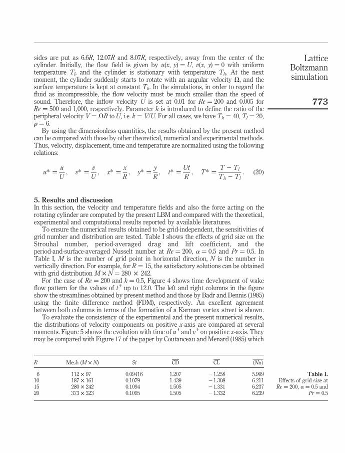
To ensure the numerical results obtained to be grid-independent, the sensitivities ofgrid number and distribution are tested. Table I shows the effects of grid size on theStrouhal number, period-averaged drag and lift coefficient, and theperiod-and-surface-averaged Nusselt number at Re ¼ 200, a ¼ 0.5 and Pr ¼ 0.5. InTable I, M is the number of grid point in horizontal direction, N is the number invertically direction. For example, for R ¼ 15, the satisfactory solutions can be obtainedwith grid distribution M £ N ¼ 280 £ 242.

For the case of Re ¼ 200 and k ¼ 0.5, Figure 4 shows time development of wakeflow pattern for the values of t* up to 12.0. The left and right columns in the figureshow the streamlines obtained by present method and those by Badr and Dennis (1985)using the finite difference method (FDM), respectively. An excellent agreementbetween both columns in terms of the formation of a Karman vortex street is shown.

To evaluate the consistency of the experimental and the present numerical results,the distributions of velocity components on positive x-axis are compared at severalmoments. Figure 5 shows the evolution with time of u* and v * on positive x-axis. Theymay be compared with Figure 17 of the paper by Coutanceau and Menard (1985) which

R Mesh (M £ N) St CD CL kNul

6 112 £ 97 0.09416 1.207 21.258 5.99910 187 £ 161 0.1079 1.439 21.308 6.21115 280 £ 242 0.1094 1.505 21.331 6.23720 373 £ 323 0.1095 1.505 21.332 6.239

Table I.Effects of grid size atRe ¼ 200, a ¼ 0.5 and

Pr ¼ 0.5

LatticeBoltzmannsimulation

773

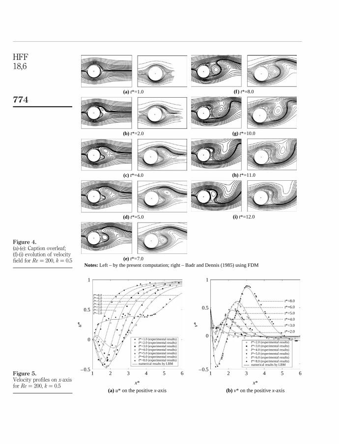
Figure 4.(a)-(e): Caption overleaf;(f)-(i) evolution of velocityfield for Re ¼ 200, k ¼ 0.5

(a) t*=1.0

(b) t*=2.0

(c) t*=4.0

(d) t*=5.0

(e) t*=7.0 Notes: Left – by the present computation; right – Badr and Dennis (1985) using FDM

(f ) t*=8.0

(g) t*=10.0

(h) t*=11.0

(i) t*=12.0

Figure 5.Velocity profiles on x-axisfor Re ¼ 200, k ¼ 0.5

(b) v* on the positive x-axis

1

0.5

0

–0.51 2 3 4 5 6

v*

x*x*

(a) u* on the positive x-axis

1

0.5

0

–0.51 2 3 4 5 6

t*=4.0t*=3.0t*=2.0

u*

t*=1.0

t*=1.0 (experimental results)t*=2.0 (experimental results)t*=3.0 (experimental results)t*=4.0 (experimental results)t*=5.0 (experimental results)t*=6.0 (experimental results)t*=8.0 (experimental results)numerical results by LBM

t*=2.0 (experimental results)t*=3.0 (experimental results)t*=4.0 (experimental results)t*=5.0 (experimental results)t*=6.0 (experimental results)t*=8.0 (experimental results)numerical results by LBM

t*=8.0t*=6.0t*=5.0

t*=4.0

t*=3.0

t*=2.0

t*=8.0

t*=6.0

t*=5.0

HFF18,6

774

indicate a good measure of quantitative agreement. Some representative points takenfrom the experimental study (Coutanceau and Menard, 1985) are shown in Figure 5 toillustrate the degree of the quantitative comparison.

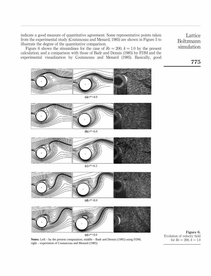
Figure 6 shows the streamlines for the case of Re ¼ 200, k ¼ 1.0 by the presentcalculation; and a comparison with those of Badr and Dennis (1985) by FDM and theexperimental visualization by Coutanceau and Menard (1985). Basically, good

Figure 6.Evolution of velocity field

for Re ¼ 200, k ¼ 1.0

(a) t*=4.0

(b) t*=6.0

(c) t*=6.5

(d) t*=8.0

(e) t*=9.0

Notes: Left – by the present computation; middle – Badr and Dennis (1985) using FDM;right – experiment of Coutanceau and Menard (1985)

LatticeBoltzmannsimulation

775

agreements can be identified except the streamlines at t* ¼ 6.0. At this moment, asshown in Figure 6(b), the streamline shows that two vortices which do not appear inthe corresponding plot by FDM have been formed over the surface of the circularcylinder. In order to test which result is more accurate, two numerical results att* ¼ 6.0 are compared, respectively, with the corresponding experimental result ofCoutanceau and Menard (1985). The comparison shows that two vortices appearing inthe present simulation are correct, as it was observed by the experiment when t* ¼ 6.0.This demonstrates that the present simulation based on the LBM is more realistic thanthat by FDM in reproducing the flow details.

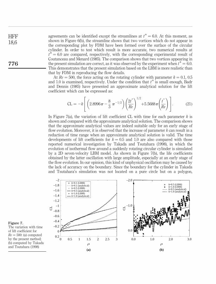
At Re ¼ 500, the force acting on the rotating cylinder with parameter k ¼ 0.1, 0.5and 1.0 is examined, respectively. Under the condition that t* is small enough, Badrand Dennis (1985) have presented an approximate analytical solution for the liftcoefficient which can be expressed as:

CL ¼ 2k 2:8996p28

3p21=2

� �2t

*

Re

!1=2

þ5:5688pt*

Re

!24

35: ð21Þ

In Figure 7(a), the variation of lift coefficient CL with time for each parameter k isshown and compared with the approximate analytical solution. The comparison showsthat the approximate analytical values are indeed suitable only for an early stage offlow evolution. Moreover, it is observed that the increase of parameter k can result in areduction of time range when an approximate analytical solution is valid. The timedevelopments of lift coefficients for k ¼ 0.5 and 1.0 are also compared with thosereported numerical investigation by Takada and Tsutahara (1998), in which theevolution of isothermal flow around a suddenly rotating circular cylinder is simulatedby a 2D seven-velocity LBM model. As shown in Figure 7(b), the life coefficientsobtained by the latter oscillation with large amplitude, especially at an early stage ofthe flow evolution. In our opinion, this kind of unphysical oscillation may be caused bythe lack of accuracy on the boundary. Since the boundary for the cylinder in Takadaand Tsutahara’s simulation was not located on a pure circle but on a polygon,

Figure 7.The variation with timeof lift coefficient forRe ¼ 500: (a) computedby the present method;(b) computed by Takadaand Tsutahara (1998)

(a)

–2

–1.8

–1.6

–1.4

–1.2

–1

–0.8

–0.6

–0.4

–0.2

CL

t*

0.2

0

0.5 1.50 1 2 2.5 3

k=0.1 (LBM)k=0.1 (analytical)

k=1.0 (LBM)k=1.0 (analytical)

k=0.5 (LBM)k=0.5 (analytical)

(b)

–2.0

–1.0

0.0

0.0

CL

1.0 2.0

t*

3.0

k=1.0 (LBM)

k=1.0 (analytical)

k=0.5 (LBM)

k=0.5 (analytical)

HFF18,6

776

the cylinder must occupy more lattice units so that the polygon may approach a circle.This kind of treatment has factitiously changed the real geometry of the boundary andtherefore led to a reduction in computational accuracy. The comparison shows that thepresent method for dealing with curved boundary can overcome the limitationmentioned above so that is more accurate.

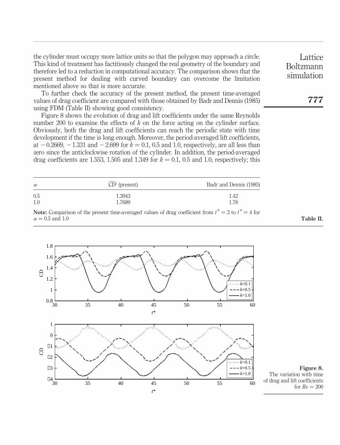
To further check the accuracy of the present method, the present time-averagedvalues of drag coefficient are compared with those obtained by Badr and Dennis (1985)using FDM (Table II) showing good consistency.

Figure 8 shows the evolution of drag and lift coefficients under the same Reynoldsnumber 200 to examine the effects of k on the force acting on the cylinder surface.Obviously, both the drag and lift coefficients can reach the periodic state with timedevelopment if the time is long enough. Moreover, the period-averaged lift coefficients,at 20.2669, 21.331 and 22.699 for k ¼ 0.1, 0.5 and 1.0, respectively, are all less thanzero since the anticlockwise rotation of the cylinder. In addition, the period-averageddrag coefficients are 1.553, 1.505 and 1.349 for k ¼ 0.1, 0.5 and 1.0, respectively; this

a CD0 (present) Badr and Dennis (1985)

0.5 1.3943 1.421.0 1.7689 1.78

Note: Comparison of the present time-averaged values of drag coefficient from t * ¼ 3 to t * ¼ 4 fora ¼ 0.5 and 1.0 Table II.

Figure 8.The variation with time

of drag and lift coefficientsfor Re ¼ 200

1.8

1.6

1.4

1.2

1

1

0

−1

−2

−3

−4

0.830 35

CD

CD

40 45 50 55 60

k=0.1k=0.5k=1.0

k=0.1k=0.5k=1.0

30 35 40 45 50 55 60

t*

t*

LatticeBoltzmannsimulation

777

indicates that the increase of k from 0.1 to 1.0 results in a decrease of period-averageddrag coefficient.

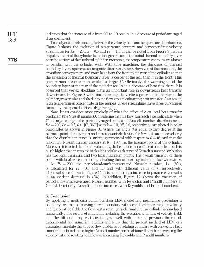
To analysis the relationship between the velocity field and temperature distributions,Figure 9 shows the evolution of temperature contours and corresponding velocitystreamlines for Re ¼ 200, k ¼ 0.5 and Pr ¼ 1.0. It can be noted from Figure 9 that animpulsive start of the cylinder leads to a generation of the initial thermal boundary layernear the surface of the isotheral cylinder; moreover, the temperature contours are almostin parallel with the cylinder wall. With time marching, the thickness of thermalboundary layer experiences a magnification everywhere. However, at the same time, thecrossflow conveys more and more heat from the front to the rear of the cylinder so thatthe extension of thermal boundary layer is deeper at the rear than it in the front. Thisphenomenon becomes more evident a larger t*. Obviously, the warming up of theboundary layer at the rear of the cylinder results in a decrease of heat flux there. It isobserved that vortex shedding plays an important role in downstream heat transferdownstream. In Figure 9, with time marching, the vortices generated at the rear of thecylinder grow in size and shed into the flow stream enhancing heat transfer. As a result,high temperatures concentrate in the regions where streamlines have large curvaturescaused by the opened vortices (Figure 9(g)-(j)).

Now, let us consider more precisely of what the effect of k on local heat transfercoefficient (the Nusselt number). Considering that the flow can reach a periodic state whent* is large enough, the period-averaged values of Nusselt number distributions atRe ¼ 200, Pr ¼ 0.5, u [ [08, 3608] with k ¼ 0.0, 0.5, 1.0, respectively, are plotted in polarcoordinates as shown in Figure 10. Where, the angle u is equal to zero degree at therearmost point of the cylinder and increases anticlockwise. For k ¼ 0, it can be seen clearlythat the distribution curve is strictly symmetrical with respect to u ¼ 08, and that themaximum Nusselt number appears at u ¼ 1808, i.e. the foremost point of the cylinder.Moreover, it is noted that for all values of k, the heat transfer coefficient on the front side ismuch higher than that on the back side and also each curve of Nusselt number distributionhas two local minimum and two local maximum points. The overall tendency of thesepoints with local extrema is to migrate along the surface of cylinder anticlockwise with k.

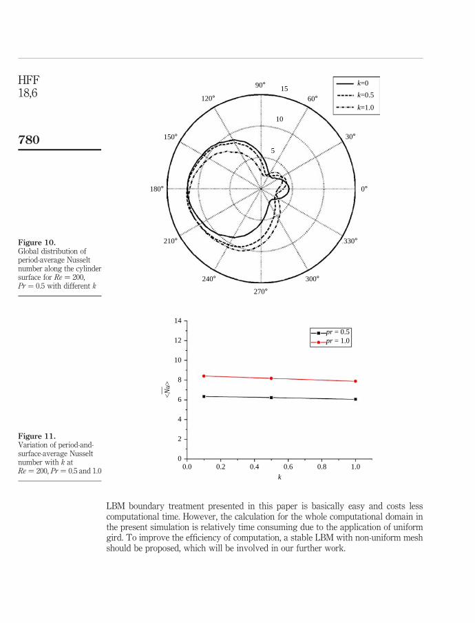
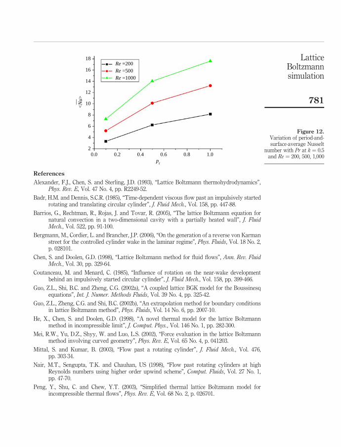
At Re ¼ 200, the period-and-surface-averaged Nusselt number, i.e. kNul,is calculated for Pr ¼ 0.5 and 1.0 and with different value of k, respectively.The results are shown in Figure 11. It is noted that an increase in parameter k resultsin an evident decrease in kNul. In addition, Figure 12 shows the variation ofperiod-and-surface-averaged Nusselt number with Reynolds and Prandtl numbers atk ¼ 0.5. Obviously, Nusselt number increases with Reynolds and Prandtl numbers.

6. ConclusionBy applying a multi-distribution function LBM model and meanwhile presenting aboundary treatment of moving curved boundary with second-order accuracy for velocityand temperature fields, the flow past a rotating isothermal circular cylinder is simulatednumerically. The results of simulation including the evolution with time of velocity field,and the lift and drag coefficients agree well with those of previous theoretical,experimental and numerical studies and show that the present method of LBM canaccurately simulate this type of flow problems of rotating cylinders with convective heattransfer. It is found that a higher Nusselt number can be obtained by either decreasing thevelocity ratio of rotating to inflow or increasing Reynolds and Prandtl numbers.

HFF18,6

778

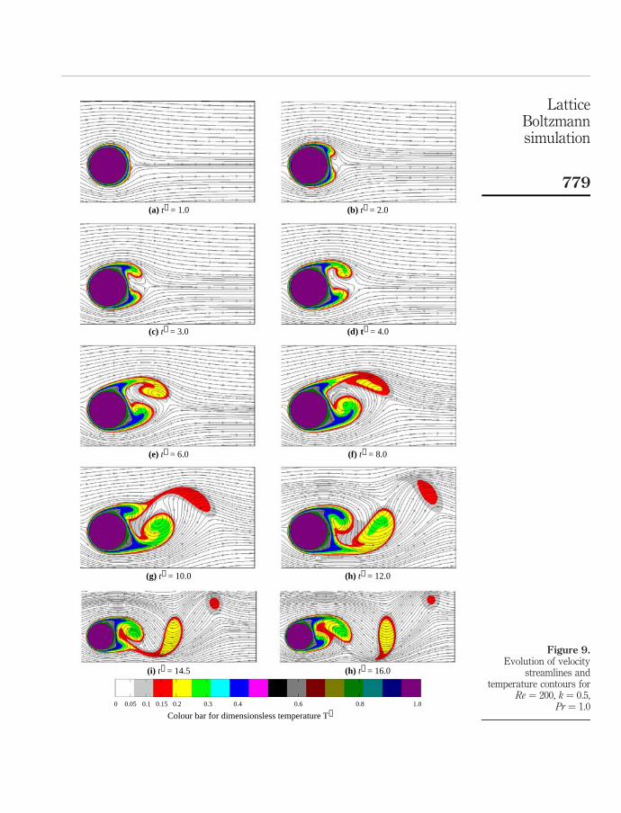
Figure 9.Evolution of velocity

streamlines andtemperature contours for

Re ¼ 200, k ¼ 0.5,Pr ¼ 1.0

(a) t∗ = 1.0

(c) t∗ = 3.0

(e) t∗ = 6.0

(g) t∗ = 10.0

(i) t∗ = 14.5

0 0.05 0.15 0.2 0.3 0.4 0.6 0.8 1.0

Colour bar for dimensionsless temperature T∗0.1

(b) t∗ = 2.0

(d) t∗ = 4.0

(f) t∗ = 8.0

(h) t∗ = 12.0

(h) t∗ = 16.0

LatticeBoltzmannsimulation

779

LBM boundary treatment presented in this paper is basically easy and costs lesscomputational time. However, the calculation for the whole computational domain inthe present simulation is relatively time consuming due to the application of uniformgird. To improve the efficiency of computation, a stable LBM with non-uniform meshshould be proposed, which will be involved in our further work.

Figure 10.Global distribution ofperiod-average Nusseltnumber along the cylindersurface for Re ¼ 200,Pr ¼ 0.5 with different k

90°

60°

30°

0°

330°

300°

270°

240°

210°

180°

150°

120°15

10

5

k=0

k=0.5

k=1.0

Figure 11.Variation of period-and-surface-average Nusseltnumber with k atRe ¼ 200, Pr ¼ 0.5 and 1.0

14

12

10

8

6

— <N

u>

4

2

00.0 0.2 0.4 0.6 0.8 1.0

k

pr = 0.5pr = 1.0

HFF18,6

780

References

Alexander, F.J., Chen, S. and Sterling, J.D. (1993), “Lattice Boltzmann thermohydrodynamics”,Phys. Rev. E, Vol. 47 No. 4, pp. R2249-52.

Badr, H.M. and Dennis, S.C.R. (1985), “Time-dependent viscous flow past an impulsively startedrotating and translating circular cylinder”, J. Fluid Mech., Vol. 158, pp. 447-88.

Barrios, G., Rechtman, R., Rojas, J. and Tovar, R. (2005), “The lattice Boltzmann equation fornatural convection in a two-dimensional cavity with a partially heated wall”, J. FluidMech., Vol. 522, pp. 91-100.

Bergmann, M., Cordier, L. and Brancher, J.P. (2006), “On the generation of a reverse von Karmanstreet for the controlled cylinder wake in the laminar regime”, Phys. Fluids, Vol. 18 No. 2,p. 028101.

Chen, S. and Doolen, G.D. (1998), “Lattice Boltzmann method for fluid flows”, Ann. Rev. FluidMech., Vol. 30, pp. 329-64.

Coutanceau, M. and Menard, C. (1985), “Influence of rotation on the near-wake developmentbehind an impulsively started circular cylinder”, J. Fluid Mech., Vol. 158, pp. 399-466.

Guo, Z.L., Shi, B.C. and Zheng, C.G. (2002a), “A coupled lattice BGK model for the Boussinesqequations”, Int. J. Numer. Methods Fluids, Vol. 39 No. 4, pp. 325-42.

Guo, Z.L., Zheng, C.G. and Shi, B.C. (2002b), “An extrapolation method for boundary conditionsin lattice Boltzmann method”, Phys. Fluids, Vol. 14 No. 6, pp. 2007-10.

He, X., Chen, S. and Doolen, G.D. (1998), “A novel thermal model for the lattice Boltzmannmethod in incompressible limit”, J. Comput. Phys., Vol. 146 No. 1, pp. 282-300.

Mei, R.W., Yu, D.Z., Shyy, W. and Luo, L.S. (2002), “Force evaluation in the lattice Boltzmannmethod involving curved geometry”, Phys. Rev. E, Vol. 65 No. 4, p. 041203.

Mittal, S. and Kumar, B. (2003), “Flow past a rotating cylinder”, J. Fluid Mech., Vol. 476,pp. 303-34.

Nair, M.T., Sengupta, T.K. and Chauhan, US (1998), “Flow past rotating cylinders at highReynolds numbers using higher order upwind scheme”, Comput. Fluids, Vol. 27 No. 1,pp. 47-70.

Peng, Y., Shu, C. and Chew, Y.T. (2003), “Simplified thermal lattice Boltzmann model forincompressible thermal flows”, Phys. Rev. E, Vol. 68 No. 2, p. 026701.

Figure 12.Variation of period-and-surface-average Nusselt

number with Pr at k ¼ 0.5and Re ¼ 200, 500, 1,000

18

<N

u>—

16

14

12

10

8

6

4

20.0 0.2 0.4 0.6 0.8 1.0

pr

Re =200Re =500Re =1000

LatticeBoltzmannsimulation

781

Shi, Y., Zhao, T.S. and Guo, Z.L. (2004), “Thermal lattice Bhatnagar-Gross-Krook model for flowswith viscous heat dissipation in the incompressible limit”, Phys. Rev. E, Vol. 70 No. 6,p. 066310.

Takada, N. and Tsutahara, M. (1998), “Evolution of viscous flow around a suddenly rotatingcircular cylinder in the lattice Boltzmann method”, Comput. Fluids, Vol. 27 No. 7,pp. 807-28.

Teixeira, C., Chen, H.D. and Freed, D.M. (2000), “Multi-speed thermal lattice Boltzmann methodstabilization via equilibrium under-relaxation”, Comput. Phys. Commun., Vol. 129 Nos 1/3,pp. 207-26.

Watari, M. and Tsutahara, M. (2004), “Possibility of constructing a multispeedBhatnagar-Gross-Krook thermal model of the lattice Boltzmann method”, Phys. Rev. E,Vol. 70 No. 1, p. 016703.

Yu, D.Z., Mei, R.W, Luo, L.S. and Wei, S. (2003), “Viscous flow computations with the method oflattice Boltzmann equation”, Prog. Aerosp. Sci., Vol. 39, pp. 329-67.

Corresponding authorY.Y. Yan can be contacted at: yuying.yan@nottingham.ac.uk

HFF18,6

782

To purchase reprints of this article please e-mail: reprints@emeraldinsight.comOr visit our web site for further details: www.emeraldinsight.com/reprints