lattice boltzmann method - ndl.ethernet.edu.et
TRANSCRIPT


Lattice Boltzmann Methodand its Applications in Engineering
8806_9789814508292_tp.indd 1 1/3/13 5:21 PM

Advances in Computational Fluid Dynamics
Editors-in-Chief: Chi-Wang Shu (Brown University, USA) andChang Shu (National University of Singapore,
Singapore)
Published
Vol. 2 Adaptive High-Order Methods in Computational Fluid Dynamicsedited by Z. J. Wang (Iowa State University, USA)
Vol. 3 Lattice Boltzmann Method and Its Applications in Engineeringby Zhaoli Guo (Huazhong University of Science and Technology, China)and Chang Shu (National University of Singapore, Singapore)
Forthcoming
Vol. 1 Computational Methods for Two-Phase Flowsby Peter D. M. Spelt (Imperial College London, UK),Stephen J. Shaw (X'ian Jiaotong – University of Liverpool, Suzhou,China) & Hang Ding (University of California, Santa Barbara, USA)
Chelsea - Lattice Boltzmann Method.pmd 3/1/2013, 12:01 PM1

N E W J E R S E Y • L O N D O N • S I N G A P O R E • B E I J I N G • S H A N G H A I • H O N G K O N G • TA I P E I • C H E N N A I
World Scientific
Zhaoli GuoHuazhong University of Science and Technology, China
Chang ShuNational University of Singapore, Singapore
Computational Fluid Dynamics Advances in Vol.
3
Lattice Boltzmann Methodand its Applications in Engineering
8806_9789814508292_tp.indd 2 1/3/13 5:21 PM

Published by
World Scientific Publishing Co. Pte. Ltd.
5 Toh Tuck Link, Singapore 596224
USA office: 27 Warren Street, Suite 401-402, Hackensack, NJ 07601
UK office: 57 Shelton Street, Covent Garden, London WC2H 9HE
British Library Cataloguing-in-Publication Data
A catalogue record for this book is available from the British Library.
Advances in Computational Fluid Dynamics — Vol. 3
LATTICE BOLTZMANN METHOD AND ITS APPLICATIONS IN ENGINEERING
Copyright © 2013 by World Scientific Publishing Co. Pte. Ltd.
All rights reserved. This book, or parts thereof, may not be reproduced in any form or by any means,
electronic or mechanical, including photocopying, recording or any information storage and retrieval
system now known or to be invented, without written permission from the Publisher.
For photocopying of material in this volume, please pay a copying fee through the Copyright
Clearance Center, Inc., 222 Rosewood Drive, Danvers, MA 01923, USA. In this case permission to
photocopy is not required from the publisher.
ISBN 978-981-4508-29-2
Printed in Singapore.
Chelsea - Lattice Boltzmann Method.pmd 3/1/2013, 12:01 PM2

v
Dedication
The authors would like to devote this book to their families for their
infinite patience and encouragement.

This page intentionally left blankThis page intentionally left blank

vii
Preface
The fluid flows can be basically described at three levels: macroscopic,
mesoscopic and microscopic. In the macroscopic level, the physical
conservation laws of mass, momentum and energy are applied to a
control volume to establish a set of partial differential equations (mass,
momentum and energy equations) for governing the fluid flow. The
conventional computational fluid dynamics (CFD) is to solve these
governing equations by using various numerical methods. In contrast, the
lattice Boltzmann method (LBM), developed about two decades ago, is
an approach at mesoscopic level. LBM studies the microdynamics of
fictitious particles by using simplified kinetic models. It provides an
alternative way for simulating fluid flows. The kinetic nature brings
many distinctive features to LBM such as the clear picture of streaming
and collision processes of simulated fluid particles, the simple algorithm
structure, the easy implementation of boundary conditions, and the
natural parallelism. These appealing features make LBM a powerful
numerical tool for simulating fluid systems involving complex physics.
The past two decades have witnessed the rapid development of LBM
in fundamental theories, basic models, and wide applications. Indeed, the
method has gained much success in modelling and simulating various
complicated flows. Several books have been published to address the
need of students and researchers in the study, development and
applications of LBM. The present book has the following unique features
to distinguish it from previous ones. At first, this book is comprehensive
in scope. It presents a systemic and self-contained description of
LBM, including the basic idea, model construction, algorithm and
implementation, and various applications. Secondly, it covers the state-
of-the-art development and applications of LBM, and some areas in this

viii Lattice Boltzmann Method and Its Applications in Engineering
book such as treatments of body force, acceleration techniques,
initialization methods, and applications in micro flows and moving
boundary flows, have not been addressed in the previous books. Thirdly,
through some sample examples, the book provides step by step
implementation of algorithms, treatments of boundary conditions and
computer codes. It is believed that this part of work is useful to the
graduate students and beginners in the area.
The authors of this book, Drs Zhaoli GUO and Chang SHU, have
been working on the development and applications of LBM for more
than 12 years. They gained much experience from their research in this
area. Indeed, many parts of the book are from their research work. For
this book, Guo contributed Chapters 1-5, 7, 8 and most parts of Chapter 9,
and Shu contributed Chapter 6, the section of Taylor series expansion
and least square-based LBM as well as the stencil adaptive LBM in
Chapter 3, and the section of immersed boundary-lattice Boltzmann
method in Chapter 9.
This book is written for different levels of readers. For students and
beginners, the book is easy to understand and follow. The detailed
description of algorithms and implementation of initial/boundary
conditions as well as sample applications will give a great help to them.
The book will also attract experts in the LBM community. The detailed
presentation of physical origins, mathematical derivations and theoretical
analysis of various LB models provides useful information for
researchers in the area. Furthermore, the comprehensive references
enable the reader to find more sources if further information is needed.
Finally, the authors would like to thank their research assistants for
preparing some of the materials to write this book. Guo also expresses
his acknowledgement for the finical supports from the National Natural
Science Foundation of China (51125024) and the National Basic
Research Programme of China (2011CB707300).
Z. L. Guo and C. Shu

ix
Contents
Dedication ..................................................................................................................... v
Preface .......................................................................................................................... vii
Chapter 1 Introduction ............................................................................................... 1
1.1 Description of Fluid System at Different Scales ................................ 1
1.1.1 Microscopic description: molecular dynamics ......................... 1
1.1.2 Mesoscopic description: kinetic theory .................................... 3
1.1.3 Macroscopic description: hydrodynamic equations ................. 6
1.2 Numerical Methods for Fluid Flows .................................................. 8
1.3 History of LBE ................................................................................... 10
1.3.1 Lattice gas automata ................................................................ 10
1.3.2 From LGA to LBE ................................................................... 16
1.3.3 From continuous Boltzmann equation to LBE ......................... 18
1.4 Basic Models of LBE ......................................................................... 19
1.4.1 LBGK models .......................................................................... 19
1.4.2 From LBE to the Navier-Stokes equations: Chapman-Enskog
expansion ................................................................................. 21
1.4.3 LBE models with multiple relaxation times ............................. 25
1.5 Summary ............................................................................................ 33
Chapter 2 Initial and Boundary Conditions for Lattice Boltzmann Method............... 35
2.1 Initial Conditions ................................................................................ 35
2.1.1 Equilibrium scheme ................................................................. 35
2.1.2 Non-equilibrium scheme.......................................................... 36
2.1.3 Iterative method ....................................................................... 38
2.2 Boundary Conditions for Flat Walls................................................... 40
2.2.1 Heuristic schemes .................................................................... 40
2.2.2 Hydrodynamic schemes ........................................................... 43
2.2.3 Extrapolation schemes ............................................................. 46
2.3 Boundary Conditions for Curved Walls ............................................. 49
2.3.1 Bounce-back schemes .............................................................. 50
2.3.2 Fictitious equilibrium schemes ................................................ 51

x Lattice Boltzmann Method and Its Applications in Engineering
2.3.3 Interpolation schemes .............................................................. 52
2.3.4 Non-equilibrium extrapolation scheme .................................... 55
2.4 Pressure Boundary Conditions ........................................................... 56
2.4.1 Periodic boundary conditions .................................................. 56
2.4.2 Hydrodynamic schemes ........................................................... 58
2.4.3 Extrapolation schemes ............................................................. 58
2.5 Summary ............................................................................................ 59
Chapter 3 Improved Lattice Boltzmann Models ........................................................ 61
3.1 Incompressible Models ...................................................................... 61
3.2 Forcing Schemes with Reduced Discrete Lattice Effects ................... 66
3.2.1 Scheme with modified equilibrium distribution function ........ 66
3.2.2 Schemes with a forcing term.................................................... 67
3.2.3 Analysis of the forcing schemes .............................................. 72
3.2.4 Forcing scheme for MRT-LBE ................................................ 76
3.3 LBE with Nonuniform Grids .............................................................. 78
3.3.1 Grid-refinement and multi-block methods ............................... 78
3.3.2 Interpolation methods .............................................................. 83
3.3.3 Finite-difference based LBE methods ...................................... 84
3.3.4 Finite-volume based LBE methods .......................................... 90
3.3.5 Finite-element based LBE methods ......................................... 93
3.3.6 Taylor series expansion and least square based methods ......... 97
3.4 Accelerated LBE Methods for Steady Flows ..................................... 103
3.4.1 Spectrum analysis of the hydrodynamic equations of the
standard LBE ........................................................................... 104
3.4.2 Time-independent methods ...................................................... 105
3.4.3 Time-dependent methods ......................................................... 107
3.5 Summary ............................................................................................ 114
Chapter 4 Sample Applications of LBE for Isothermal Flows ................................... 117
4.1 Algorithm Structure of LBE ............................................................... 117
4.2 Lid-Driven Cavity Flow ..................................................................... 130
4.3 Flow around a Fixed Circular Cylinder .............................................. 133
4.4 Flow around an Oscillating Circular Cylinder with a Fixed
Downstream One ................................................................................ 138
4.5 Summary ............................................................................................ 144
Chapter 5 LBE for Low Speed Flows with Heat Transfer ......................................... 145
5.1 Multi-speed Models ........................................................................... 146
5.1.1 Low-order models .................................................................... 146
5.1.2 High-order models ................................................................... 152
5.2 MS-LBE Models Based on Boltzmann Equation ............................... 155
5.2.1 Hermite expansion of distribution function ............................. 155

Contents xi
5.2.2 Temperature/flow-dependent discrete velocities ..................... 158
5.2.3 Temperature-dependent discrete velocities .............................. 158
5.2.4 Constant discrete velocities ..................................................... 160
5.2.5 MS-LBGK models based on DVBE with constant discrete
velocities .................................................................................. 162
5.3 Off-Lattice LBE Models .................................................................... 165
5.4 MS-LBE Models with Adjustable Prandtl Number ............................ 168
5.5 DDF-LBE Models without Viscous Dissipation and Compression
Work .................................................................................................. 172
5.5.1 DDF-LBE based on multi-component models ......................... 172
5.5.2 DDF-LBE for non-ideal gases ................................................. 174
5.5.3 DDF-LBE for incompressible flows ........................................ 175
5.6 DDF-LBE with Viscous Dissipation and Compression Work –
Internal Energy Formulation .............................................................. 177
5.6.1 Internal energy distribution function ........................................ 177
5.6.2 Lattice Boltzmann equations.................................................... 179
5.6.3 Some simplified models........................................................... 181
5.7 DDF-LBE with Viscous Dissipation and Compression Work –
Total Energy Formulation .................................................................. 183
5.7.1 Total energy distribution function............................................ 183
5.7.2 Discrete velocity model ........................................................... 187
5.7.3 Lattice Boltzmann equations.................................................... 192
5.8 Hybrid LBE Models ........................................................................... 194
5.9 Summary ............................................................................................ 196
Chapter 6 LBE for Compressible Flows .................................................................... 197
6.1 Limitation of Conventional LBE Models for Compressible
Flows .................................................................................................. 198
6.2 Conventional Equilibrium Function-based LBE Models for
Compressible Flows ........................................................................... 200
6.3 Circular Function-based LBE Models for Compressible Flows ......... 207
6.3.1 Definition of circular equilibrium function .............................. 208
6.3.2 Distribution of circular function to lattice points in
velocity space .......................................................................... 211
6.4 Delta Function-based LBE Models for Compressible Flows ............. 217
6.5 Direct Derivation of Equilibrium Distribution Functions from
Conservation of Moments .................................................................. 221
6.6 Solution of Discrete Velocity Boltzmann Equation ........................... 225
6.7 Lattice Boltzmann Flux Solver for Solution of Euler Equations ........ 228
6.8 Some Sample Applications ................................................................ 232
6.9 Summary ............................................................................................ 235

xii Lattice Boltzmann Method and Its Applications in Engineering
Chapter 7 LBE for Multiphase and Multi-component Flows ..................................... 239
7.1 Color Models ..................................................................................... 240
7.1.1 LBE model for immiscible fluids ............................................ 240
7.1.2 LBE model for miscible fluids ................................................. 243
7.2 Pseudo-Potential Models .................................................................... 245
7.2.1 Shan-Chen model .................................................................... 245
7.2.2 Shan-Doolen model ................................................................. 247
7.2.3 Numerical schemes for interaction force ................................. 249
7.3 Free Energy Models ........................................................................... 251
7.3.1 Models for single component non-ideal fluid flows ................ 251
7.3.2 Model for binary fluid flows .................................................... 254
7.3.3 Galilean invariance of the free-energy LBE models ................ 256
7.4 LBE Models Based on Kinetic Theories ............................................ 258
7.4.1 Models for single-component multiphase flows ...................... 258
7.4.2 Models for multi-component flows.......................................... 268
7.4.3 Models for non-ideal gas mixtures........................................... 278
7.5 Summary ............................................................................................ 284
Chapter 8 LBE for Microscale Gas Flows ................................................................. 287
8.1 Introduction ........................................................................................ 287
8.2 Fundamental Issues in LBE for Micro Gaseous Flows ...................... 289
8.2.1 Relation between relaxation time and Knudsen number .......... 289
8.2.2 Slip boundary conditions ......................................................... 291
8.3 LBE for Slip Flows ............................................................................ 295
8.3.1 Kinetic boundary scheme and slip velocity ............................. 295
8.3.2 Discrete effects in the kinetic boundary conditions ................. 299
8.3.3 MRT-LBE for slip flows.......................................................... 301
8.4 LBE for Transition Flows .................................................................. 302
8.4.1 Knudsen layer .......................................................................... 302
8.4.2 LBE models with Knudsen layer effect ................................... 304
8.5 LBE for Microscale Binary Mixture Flows ........................................ 310
8.5.1 General formulation ................................................................ 310
8.5.2 Extension to micro flows ......................................................... 313
8.6 Summary ............................................................................................ 317
Chapter 9 Other Applications of LBE ........................................................................ 319
9.1 Applications of LBE for Particulate Flows ........................................ 319
9.1.1 LBE method with finite-size particles ..................................... 320
9.1.2 LBE method with point particles ............................................. 327
9.2 Applications of LBE for Flows in Porous Media ............................... 329
9.2.1 Pore-scale approach ................................................................. 331
9.2.2 REV-scale approach ................................................................ 334

Contents xiii
9.3 Applications of LBE for Turbulent Flows .......................................... 339
9.3.1 LBE-DNS approach ................................................................. 340
9.3.2 LBE-LES approach .................................................................. 343
9.3.3 LBE-RANS approach .............................................................. 350
9.4 Immersed Boundary-Lattice Boltzmann Method and Its
Applications ....................................................................................... 353
9.4.1 Conventional immersed boundary-lattice Boltzmann
method ..................................................................................... 354
9.4.2 Boundary condition-enforced immersed boundary-lattice
Boltzmann method ................................................................... 360
9.5 Summary ............................................................................................ 363
Appendix A Source Code for 2D Cavity Flow .......................................................... 365
Bibliography ................................................................................................................. 373
Index ............................................................................................................................. 397

This page intentionally left blankThis page intentionally left blank

1
Chapter 1
Introduction
1.1 Description of Fluid System at Different Scales
Fluids, such as air and water, are frequently met in our daily life.
Physically, all fluids are composed of a large set of atoms or molecules
that collide with one another and move randomly. Interactions among
molecules in a fluid are usually much weaker than those in a solid, and a
fluid can deform continuously under a small applied shear stress. Usually,
the microscopic dynamics of the fluid molecules is very complicated and
demonstrates strong inhomogeneity and fluctuations. On the other hand,
the macroscopic dynamics of the fluid, which is the average result of the
motion of molecules, is homogeneous and continuous. Therefore, it is
can be expected that mathematical models for fluid dynamics will be
strongly dependent on the length and time scales at which the fluid is
observed. Generally, the motion of a fluid can be described by three
types of mathematical models according to the observed scales, i.e.
microscopic models at molecular scale, kinetic theories at mesoscopic
scale, and continuum models at macroscopic scale.
1.1.1 Microscopic description: molecular dynamics
In microscopic models, the motion of each molecule is tracked so that its
position and momentum can be obtained. The collective dynamics of the
whole fluid system can then be computed through some statistical
methods. Usually, the molecular dynamics of the fluid is described by
Newton’s second law,
i im =r F , (1.1)

2 Lattice Boltzmann Method and Its Applications in Engineering
where m is the mass of the fluid molecule, ri is the position vector of the
molecule i, the dots represent time derivatives, and Fi is the total force
experienced by the molecule, which usually includes two parts,
1,
N
i ij i
j j i= ≠
= +∑F f G , (1.2)
where fij is the force exerted by molecule j, N is the number of molecules
in the system, and Gi is the external force such as gravity. The inter-
molecular force can be expressed in terms of an interaction potential φ(r),
(| |)ij ijφ= −∇f r , (1.3)
where rij is the displacement between molecules i and j. In microscopic
models, the inter-molecular potential plays a vital role. A widely used
model is the Lennard-Jones 12-6 potential,
12 6
( ) 4rr r
σ σφ ε
= − , (1.4)
where ε characterizes the interaction strength and σ represents the
interaction range.
By solving Eq. (1.1) we can obtain the position and velocity of each
molecule at every time, and then the macroscopic variables of the fluid,
such as density, velocity, and temperature, can be measured from the
microscopic information: A a= ⟨ ⟩. Here A is a macroscopic quantity and
a is the corresponding microscopic quantity; the symbol ⟨⋅⟩ represents
the ensemble average of a microscopic variable. The transport
coefficients of the fluid (viscosity, thermal conductivity, diffusivity, etc.)
can also be measured according to the linear response theory, which
indicates that each transport coefficient can be obtained through the
Einstein expression or the Green-Kubo relation [Rapaport, 2004].
An alternative description of the fluid is to consider the Hamiltonian
of the N-body system H H( , , )t= q p , where ( , )q p are the generalized
coordinates that constitute the phase space of the system, i.e. q = (q1, q2, …, qN) are the 3N spatial coordinates of the N molecules, and p = (p1, p2, …, pN) are the 3N conjugate momenta. H is the total energy of the system
including the kinetic energy and the potential energy due to molecular
Introduction 3
interactions. In terms of the Hamiltonian of the system, the motion of the
fluid molecules can be expressed as
H H
,i i
i i
∂ ∂= = −
∂ ∂ q p
p q, i =1, 2, …, N. (1.5)
In either the Newtonian formulation (1.1) or the Hamiltonian
formulation (1.5), the numbers of unknowns are very large (6N). Even
for a small volume of fluid in practice, the number of molecules is so
large (~1023) that it is impractical to describe the whole system with a
molecular model. Actually, even with the most advanced computer
resources, molecular dynamics method is still limited to sub-micrometer
systems.
1.1.2 Mesoscopic description: kinetic theory
A coarser description of the N-body fluid system is to make use of the
concept of probability distribution function (pdf) ( , , )Nf tq p in the phase
space, which determines the probability Nf d dq p that the state of the
system falls in the infinitesimal volume [ , ] [ , ]d d+ × +p p p q q q in the 6N
dimensional phase space. From fN , all of the statistical properties of the
molecular dynamics can be extracted. The evolution of fN follows the
Liouville equation [Harris, 1971],
1
0N
N N N Nj j
j j j
df f f f
dt t =
∂ ∂ ∂ = + ⋅ + ⋅ = ∂ ∂ ∂ ∑ p q
p q, (1.6)
or
H H
1
0N
N N N
j j j j j
f f f
t =
∂ ∂ ∂ ∂ ∂ − − = ∂ ∂ ∂ ∂ ∂ ∑
q p p q. (1.7)
From fN, we can define some reduced distribution functions,
1 1 1 1 1 1( , , , , ) ( , , , , )s s s N N N s s N NF f d d d d+ += ∫ q p q p q p q p q p q p , (1.8)
which is termed as the s-particle probability distribution function. We
can derive a chain of evolution equations for Fs (1 ≤ s ≤ N) from the
Liouville equation, which is usually called as the BBGKY (Bogoliubov–
Born–Green–Kirkwood–Yvon) hierarchy. This hierarchy is identical to

4 Lattice Boltzmann Method and Its Applications in Engineering
the original Liouville equation completely. In this chain, the first
equation for the single-particle pdf contains the two-particle pdf, the
second equation for the two-particle pdf contains the three-particle pdf,
and generally the s-th equation for the s-particle pdf contains ( 1)s + -th
pdf. Therefore, the BBGKY hierarchy is fully coupled, and the
difficulties of solving it are the same as solving the Liouville equations.
However, under some assumptions, the BBGKY hierarchy can be
truncated at certain orders so that a smaller set of equations can be
obtained to approximate the original chain. Actually, this approach has
served as a common strategy for developing kinetic equations in many
applications of kinetic theory. Particularly, the approximation equation
truncated at the first order leads to the well known Boltzmann equation
for the velocity distribution function f, which is defined as
ξ 1 1 1( , , ) ( , , )f t mNF t=x q p , (1.9)
where we have changed the notations from phase space to physical space:
x = q1 is the position of a particle and 1/m= pξ is its velocity. The
Boltzmann equation, which plays the central role in kinetic theory of
gases, describes the transportation of f :
ξ ( , )f
f f ft
∂+ ⋅ ∇ = Ω
∂, (1.10)
where Ω represents the rate of change in f due to binary molecular
collisions. When the velocity distribution function is obtained, the fluid
density ρ , velocity u, and internal energy e can be determined from its
moments:
ξ ξ ξ ξ2
2, , ( , ) Cf d f d e t f dρ ρ ρ= = =∫ ∫ ∫u x , (1.11)
where C is the magnitude of the particular velocity = −C uξ (In this
book, the magnitude of a vector a will be always denoted by a). The
pressure tensor and heat flux, can also be determined from f :
ξ ξ ξ ξ2
2( , , ) , ( , , )Cf t d f t d= =∫ ∫P CC x q C x . (1.12)
The evolution equations for the fluid density, velocity, and energy can be
derived from the Boltzmann equation under some assumptions.

Introduction 5
The collision operator Ω in the Boltzmann equation (1.10) is a bi-
linear integral function of f, and conserves mass, momentum, and energy:
ξ ξ ξ( ) ( , , ) 0i f t dψ =∫ x , (1.13)
where ξ 21, , / 2Cψ = (or 2ξ ) are called summational or collisional
invariants. From the Boltzmann equation, it can be shown that the
H-function, defined by ξ( ) lnH t f f d d= ∫ x , will always decrease with
time (H-theorem), i.e.,
0dH
dt≤ . (1.14)
The equality holds only and if only the system reaches its equilibrium
state, whence the distribution function is a Maxwellian one,
ξ
ξ2
( )
3/2
( )( , , ) exp
(2 ) 2eqf t
RT RT
ρ
π
− = −
ux , (1.15)
where /BR k m= is the gas constant with kB the Boltzmann constant and
m the molecular mass. At equilibrium, the collision does not take net
effects, i.e., ( ) ( )( , ) 0eq eqf fΩ = . With this knowledge, the collision operator
can be approximated with some simplified models [Harris, 1971], among
which the BGK (Bhatnagar-Gross-Krook) model [Bhatnagar et al., 1954]
is the most popular one,
( )1eq
BGK
c
f fτ
Ω = − − , (1.16)
where cτ is the relaxation time. This model reflects the overall effect of
intermolecular collisions, i.e., the distribution function relaxes to the
equilibrium state with collisions. It can be easily verified that the BGK
collision model conserves mass, momentum, and energy, and satisfies
the H-theorem. However, because only one relaxation time is used to
characterize the collision effects, this model also suffers from some
limitations. For example, the Prandtl number (Pr), which reflects the
difference between momentum exchange and energy exchange during
the collision process, is fixed at 1 in the BGK model, while the
full Boltzmann collision operator gives Pr = 2/3. Some modified
models have been proposed to overcome this problem, such as the

6 Lattice Boltzmann Method and Its Applications in Engineering
Ellipsoidal Statistical BGK model [Holway, 1966] and the Shakhov
model [1968].
1.1.3 Macroscopic description: hydrodynamic equations
At macroscopic scale, a fluid is treated as a continuum regardless of
its molecular structure and interaction; the fluid is assumed to be
continuously distributed throughout the domain of interest, having its
own properties such as density, velocity, and temperature. The molecular
properties are reflected by the transport coefficients of the fluid such as
the viscosity and thermal conductivity. A good criterion to determine if a
continuum model is acceptable is to check whether the Knudsen number
Kn of the fluid system, which is defined as the ratio of mean-free-path of
molecules (λ ) to the characteristic length (L) of the flow region, is
sufficiently small. The mean free path is the average distance of the fluid
molecules between two successive collisions. For an ideal gas composed
of hard-sphere molecules, it can be expressed as 2 1( 2 )ndλ π −= , where
n is the number density of the molecules and d is the diameter of the gas
molecule. The characteristic length is usually taken as the size of the
flow domain or objects in the flow, such as the diameter of an object in
the flow. In some cases, it is more suitable to define L based on the scale
at which a flow variable changes, e.g. /| |L ρ ρ= ∇ .
In continuum theory, the motion of fluid is described by a set of
partial differential equations (PDEs), which actually describes the
conservation laws of the fluid [Batchelor, 1967]:
( ) 0t
ρρ
∂+ ∇ ⋅ =
∂u , (1.17)
( )
( ) pt
ρρ
∂+ ∇ ⋅ = −∇ + ∇ ⋅
∂τ
uuu , (1.18)
( )
( ) :e
e pt
ρρ
∂+ ∇ ⋅ = −∇ ⋅ − ∇ ⋅ + ∇
∂τu q u u , (1.19)
where p is the pressure, τ is the deviatoric stress tensor, and q is the heat
flux. This set of equations are not closed because the variables p, τ, and q
are yet unknown. The pressure can be modeled by an equation of state,

Introduction 7
i.e. p =p(e), while the deviatoric stress tensor can be modeled by a
stress-strain constitution equation,
o
22 ( ) 2 ( )
3µ µ µ µ µ
′ ′= + ∇ ⋅ = + + ∇ ⋅ τ S u I S u I , (1.20)
where µ and µ′ are the first and second dynamic viscosities, I is the
second-order unit tensor, and S is the strain-rate tensor defined by
[ ( ) ] / 2T= ∇ + ∇S u u . Here, a tensor with a notation “ ° ” denotes the
traceless part of the original tensor. The coefficient 2 /3η µ µ′= + is
also called bulk viscosity in some textbooks, which is usually assumed to
be zero (Stokes’ hypothesis). The heat flux in Eq. (1.19) is usually
related to the temperature gradient following Fourier’s law,
κ= − ∇q T , (1.21)
where κ is the thermal conductivity. The set of equations (1.17)-(1.19)
with the constitution relations (1.20) and (1.21) are the widely used
Navier-Stokes-Fourier equations, which are also called Navier-Stokes
equations sometimes. This set of equations can be simplified in some
special cases. If the viscosity and thermal conductivity are neglected, the
Navier-Stokes equations then reduce to the Euler equations; If the fluid
density does not change with motion, i.e.,
0d
dt t
ρ ρρ
∂= + ⋅ ∇ =
∂u , (1.22)
the fluid is said to be incompressible, and the continuity equation (1.17)
becomes 0∇ ⋅ =u , and the stress tensor can be simplified as 2µ=τ S .
The compressibility of a fluid can be characterized by the Mach number
of the flow, / sM U c= , where U is the characteristic velocity of the flow
and cs is the sound speed. Usually, the fluid flow can be regarded as
incompressible when M < 0.3.
Although the conservation equations are developed phenomeno-
logicallly, it is shown that they can also be derived from the Boltzmann
equation. Actually, by multiplying the Boltzmann equation (1.10) by the
collisional invariants iψ and integrating over the molecular velocity
space, one can get Eqs. (1.17) ~ (1.19) after identifying that p= − τP I .

8 Lattice Boltzmann Method and Its Applications in Engineering
The stress tensor τ and the heat flux q can be approximated via some
asymptotic methods (e.g., Hilbert or Chapman-Enskog expansions).
In most of practical problems, the continuum model works very well.
However, with the increasing interests in nano/micro and multi-scale
problems, the continuum model becomes inadequate due to the relative
large Knudsen number of the system. In viewing that the Navier-Stokes
equations can be derived from the Boltzmann equation, some extended
hydrodynamic models beyond the Navier-Stokes model have been
developed from the Boltzmann equation from different viewpoints, such
as the Burnett equations, super-Burnett equations, Grad’s 13-moment
equations (see a recent comparison of these hydrodynamic models by
Lockerby et al. [2005]).
1.2 Numerical Methods for Fluid Flows
The mathematical models for fluid flows, either the Newtonian equation
for the vast number of molecules, or the Boltzmann equation for the
singlet distribution function, or the Navier-Stokes equations for the
macroscopic flow variables, are all extremely difficult to solve
analytically, if not impossible. Accurate numerical methods, however,
have been proven to be able to provide satisfying approximate solutions
to these equations. Particularly, with the rapid development of computer
hardware and software technology, numerical simulation has become an
important methodology for fluid dynamics.
The most successfully and popular fluid simulation method is the
Computational Fluid Dynamics (CFD) technique, which is mainly
designed to solve the hydrodynamic equations based on the continuum
assumption. In CFD, the flow domain is decomposed into a set of sub-
domains with a computational mesh, and the mathematical equations are
discretized using some numerical schemes such as finite-volume, finite-
element, or finite-difference methods, which results in an algebraic
system of equations for the discrete flow variables associated with the
computational mesh. Computation can then be carried out to find the
approximate solutions on a computer by solving the algebraic system
using some sequential or parallel algorithms. CFD has developed into a

Introduction 9
branch of fluid mechanics since 1960s, and many textbooks on different
topics in this field are available [e.g., Anderson, 1995; Ferzige and
Peric, 2002; Patankar, 1980]. There are also many free and commercial
softwares for both fundamental researches and practical engineering
applications.
With the increasing interests in micro and nano scale science and
technology, molecular dynamic simulation (MDS) techniques have also
received much attention in modern fluid mechanics. In MDS, the
movements of individual atoms or molecules of the fluid are recorded by
solving the Newtonian equations on a computer. The main advantage of
MDS is that macroscopic collective behaviors of the fluid can be directly
connected with the molecular behaviors, in which the molecular structure
and microscopic interactions can be described in a straightforward
manner. Therefore, MDS is very helpful for understanding the
fundamental microscopic mechanism of macroscopic fluid phenomena.
However, due to the vast number of atoms of the fluid, the computational
cost of MDS is rather expensive and this disadvantage limits it to
systems with a temporal scale of picoseconds and spatial scale of
nanometers.
Besides the macroscopic CFD and microscopic MDS methods,
another kind of numerical methods for fluid system is developed based
on mesoscopic models. Basically, mesoscopic methods can be classed
into two types. The first type is to solve the kinetic equations (e.g., the
Boltzmann equation) with some numerical schemes. Such methods
include the finite difference discretization of the linearized Boltzmann
equation [Kanki and Iuchi, 1973], the elementary method [Cercignani,
1988], the discrete velocity or discrete ordinate methods [Aristov, 2001;
Sone et al., 1989], the finite difference Monte Carlo method [Cheremisin,
1991], gas kinetic scheme [Xu, 1993], and lattice Boltzmann equation
(LBE) method [Benzi et al., 1992]. Another type of mesoscopic method
is to construct numerical models to simulate the physical process of some
virtual fluid particles directly. The most well-known method of such type
is the Direct Simulation Monte Carlo (DSMC) method [Bird, 1994], and
other methods of this type include the lattice gas automata (LGA)
method [Rothman and Zaleski, 1997] and the dissipative particle
dynamics (DPD) method [Hoogerbrugge and Koelman, 1992].

10 Lattice Boltzmann Method and Its Applications in Engineering
Because the underlying mathematical models have different physical
bases, the numerical methods also have their own application ranges.
CFD is very successful in continuum flows, and MDS is most suitable
for nanoscale flows. With the increasing interests in multiscale flows, the
mesoscopic method has received particular attentions in recent years,
among which the lattice Boltzmann equation (LBE) method, or lattice
Boltzmann method), is perhaps the most active topic in this field due to
some distinctive features. In addition to a large amount of journal papers
in different research fields, LBE is also a hot topic in many international
conferences on fluid dynamics, and some courses on this topic have been
set up in some universities. In the rest part of this book, we will give a
systemic introduction of this method.
1.3 History of LBE
Historically, the LBE evolved from the LGA method, which is an
artificial microscopic model for gases, and later it was shown that LBE
could also be derived from the Boltzmann equation following some
standard discretization. From the first viewpoint, LBE can be regarded as
a fluid model, while the second viewpoint indicates that LBE is just a
special numerical scheme for the Boltzmann equation. Despite of this
conceptual difference, either approach demonstrates that LBE is a
method which is quite different from the traditional CFD algorithms.
1.3.1 Lattice gas automata
LGA is the precursor of LBE, which aims to simulate fluid flows with
simple fluid models. In LGA, the fluid is treated as a set of simulated
particles residing on a regular lattice with certain symmetry properties,
where they collide and stream following some prescribed rules that
satisfy some necessary physical laws. The philosophy behind LGA is
that fluid behaviors at macroscale are nothing but statistical collective
results of the micro-dynamics of fluid molecules, and are insensitive to
the detailed information of the individual molecules. In other words,
fluids with different micro structures and interactions may have the

Introduction 11
same macroscopic phenomena. Therefore, it is possible to simulate
macroscopic flows with a fictitious micro fluid model which has simple
micro-dynamics but satisfies some necessary physical laws. LGA is just
one such fluid model, and the key requirement of a LGA model is that
the mass, momentum, and energy must be conserved during the particle
collision and streaming processes.
The first LGA model was attributed to three French scientists, Hardy,
Pomeau, and de Pazzis, which is called the HPP model after the authors
[Hardy et al., 1973a, 1973b]. This model utilizes a two-dimensional
square lattice on which the gas particles at a node can move to any of the
four nearest neighboring nodes along the lattice lines (see Fig. 1.1). The
collision of the HPP model follows the so called head-on rule, namely,
when two particles move to one same node with opposite velocities, their
velocities will turn around 90° after the collision; In any other cases, no
collision occurs and the particle velocities remain unchanged.
Mathematically, the motion of the particles in HPP model can be
described by the following discrete kinetic equation,
( , ) ( , ) ( ( , ))i i t t i in t n t C n tδ δ+ + = +x c x x , (1.23)
where ( , ) 0in t =x or 1 representing the number of particles moving with
discrete velocity ci at node x and time t, δt is the time step, Ci is the
collision operator representing the influence of particle collisions. The
1
2
3
4
Fig. 1.1. Lattice and discrete velocities of the HPP model.

12 Lattice Boltzmann Method and Its Applications in Engineering
discrete velocity set of the HPP model is given by ci = cei with e1 = (1,
0), e2 = (0, 1), e3 = (−1, 0), and e4 = (0, −1), and c = δx /δt is the lattice
speed where δx is the lattice spacing. The collision operator describing
the head-on rule can be expressed as
1 3 2 1 3 2(1 )(1 ) (1 )(1 )i i i i i i i i iC n n n n n n n n⊕ ⊕ ⊕ ⊕ ⊕ ⊕= − − − − − , (1.24)
where “⊕” represents the modulo 4 addition. It can be verified that Ci
conserves mass, momentum, and energy:
0i
i
C =∑ , 0i i
i
C =∑c , 2
02
ii
i
cC =∑ . (1.25)
The evolution of the fictitious particles can also be decomposed into two
sub-processes, i.e,
Collision: ( , ) ( , ) ( ( , ))i i in t n t C n t′ = +x x x , (1.26)
Streaming: ( , ) ( , )i i t t in t n tδ δ ′+ + =x c x . (1.27)
The flow variables such as the density, velocity, and temperature can
be obtained from the ensemble average (distribution function) of the
Boolean number i if n= ⟨ ⟩ ,
2, , ( )2
i i i i i i
i
mf f em
m RT fρ ρ ρ ρ= = = = −∑ ∑ ∑u c uc , (1.28)
where m is the molecular mass of the gas, and will be assumed to be 1
without loss of generality. It is not straightforward to compute the
ensemble average from ni , and usually it can be replaced by temporal or
spatial (or both) average in applications.
Although the microdynamics of the HPP model satisfies the basic
conservation laws, the hydrodynamics variables do not satisfy the
continuum equations due to the insufficient symmetry of the square
lattice. Actually, the HPP model was designed as a micro fluid model
rather than a computational method for hydrodynamic flows. Even
though, the basic idea behind the HPP model opens a new way for flow
computations.
The symmetry requirement on the lattice was first discovered in 1986
when Frisch, Hasslacher, and Pomeau proposed their hexagonal LGA

Introduction 13
model [Frisch et al., 1986] (and simultaneously by Wolfram [1986]),
which is now known as FHP model after the authors. This model uses a
triangular lattice, and each node has six nearest neighbours (Fig. 1.2).
The discrete velocities can be expressed as ci = c(cos θi , sin θi) with θi=
(i − 1)π/3 for i =1 ~ 6. Like in the HPP model, the state of FHP model
can be described by six Boolean numbers ni that represent the number of
particles moving with velocity ci . The collision rule of the FHP model
includes five different cases, as shown in Fig. 1.2.
It is noted that in some cases, one input state may correspond to two
possible output states (cases a and d shown in Fig. 1.2). In such cases,
each output state is chosen randomly with equal probability. As such, the
mathematical formulation of the collision operator can be written as
1 3 5 2 4 1 3 5 2 4
1 4 2 3 5 2 5 1 3 4
3 1 2 4 5
(1 )
,
i i i i i i i i i i i i i
i i i i i i i i i i i i
i i i i i i
r
C n n n n n n n n n n n n
rn n n n n n n n n n n n
n n n n n n
⊕ ⊕ ⊕ ⊕ ⊕ ⊕ ⊕ ⊕ ⊕ ⊕
⊕ ⊕ ⊕ ⊕ ⊕ ⊕ ⊕ ⊕ ⊕ ⊕
⊕ ⊕ ⊕ ⊕ ⊕
= −
+ −+
−
(1.29)
where “⊕” represents the modulo 6 addition and r is a random number
distributed uniformly in [0,1].
It can be shown that the collision operator of the FHP model leads to
a Fermi-Dirac distribution at equilibrium for the distribution function
[Frisch et al., 1987], i.e.,
( ) / 6
1 exp[ ]
eqi
i
fA B
ρ=
+ + ⋅c u , (1.30)
where A and B are the Lagrangian multipliers, which can be determined
by expanding ( )eqif into a series of u and imposing the mass and
momentum constraints (for isothermal flows) given by Eq. (1.28). The
final expression of ( )eqif for the FHP model can be written as [Frisch
et al., 1987],
( )
2 4
:1 ( )
6 2
eq i ii
s s
f Gc c
ρρ
⋅ = + +
c u Q uu, (1.31)
where 2 2/2sc c= is usually called sound speed in LGA (and LBE),
G(ρ)=(6 − 2ρ)/(6 − ρ), and 2i i i sc= −Q c c I . With this expanded equilibrium

14 Lattice Boltzmann Method and Its Applications in Engineering
distribution function (EDF), it can be shown that the fluid density and
velocity of the FHP model satisfy the following hydrodynamic equations
in the incompressible limit (ρ → ρ0):
0∇ ⋅ =u , (1.32)
Fig. 1.2. FHP model and the collision rule.

Introduction 15
(0) 20
0
( )( )p
gt
ρ νρ
∂ ∇+ ⋅ ∇ = − + ∇
∂u
u u u , (1.33)
where
2
2
21sp c g
c
= − u
ρ , (0) 2
30
1 1
(1 ) 4s tc
sν δ
ρ
= − −
,
with s = ρ0/6, g = (ρ0 − 3)/(ρ0 − 6). In general g ≠ 1 and this leads to the
breakdown of the Galilean invariance. However, the Galilean invariance
can be restored by rescaling the time, i.e., t→ t/g(ρ0), and the momentum
equation becomes
2Pt
∂+ ⋅ ∇ = −∇ + ∇
∂u u u
uν , (1.34)
where P = p/ρ0g and ν = ν(0)/g. Equation (1.34) resembles the incom-
pressible Navier-Stokes equation very closely, except that the rescaled
pressure P depends on the velocity. This is somewhat unphysical, but as
the Mach number is small, the pressure p satisfies an equation of state of
ideal gas, 2sp c ρ= .
Both the HPP and FHP models are designed for two-dimensional
(2D) flows. It is not an easy task to find a 3D lattice with sufficient
symmetries. On the other hand, it was shown that the 4D Face-Centered-
Hyper-Cube (FCHC) lattice, which contains 24 discrete velocities with
magnitude 2c, has the desired properties [d'Humières et al., 1986]. By
projecting back onto three-dimensional, one can obtain a set of 3D
discrete velocities that have the required symmetries. However, the
number of possible states of the collision rule in the FCHC model is still
very huge (224!), so it is a tough job to design an efficient collision rule
for it, and this was also the target of many subsequent works. The
theoretical foundation of the FCHC model was accomplished by
Wolfram [1986] and Frisch et al. [1987], and after that, many
applications have been conducted to complex flows such as multiphase
systems and flows in porous media.
The implementation of a LGA model is straightforward, just a
following of the collision-streaming paradigm. Particularly, the Boolean
representation of the basic variable in LGA means that the computation
can be realized with pure Boolean operations without round-off errors,

16 Lattice Boltzmann Method and Its Applications in Engineering
and the computation will be unconditional stable. Furthermore, because
the update of the state at each node is completely local, the algorithm
exhibits natural parallelism and thus is very suitable for parallel
computations. Despite these advantages, the LGA method also has some
disadvantages, such as the statistical noise arising from the Boolean
variables, the violation of the Galilean invariance, and the dependence of
velocity of the pressure. Historically, it is these unexpected features that
motivate the invention of the lattice Boltzmann method.
1.3.2 From LGA to LBE
The LBE first appeared in the analysis of the hydrodynamic behaviors of
the LGA model [Frisch et al., 1987]. But it was McNamara and Zanetti
who first proposed using LBE as a computation method [1988]. In order
to reduce the statistical noise in LGA, they replaced the Boolean variable
ni by the real-valued distribution function fi directly, and the collision
rule for fi is the same form as that for ni . The evolution equation of this
method (MZ model) can be written as
( , ) ( , ) ( ( , ))i i i it tf t f t f tδ δ+ + − = Ωx c x x , (1.35)
where the term on the right hand is the collision operator, ( )i fΩ =
( ) ( ) ( )i i iC n C n C f⟨ ⟩ ≈ ⟨ ⟩ = .
Although the MZ model can remove the statistical noise effectively,
the collision operator is still rather complicated. Soon after the MZ
model, Higuera and Jimenez proposed an improved version (HJ model)
[1989]. They showed that the collision operator in the MZ model could
be approximated by a linearized one by assuming that fi is close to its
equilibrium,
( ) ( )eq neqi i if f f= + , (1.36)
where ( )eqif is the expansion of the Fermi-Dirac distribution function with
a similar formulation as Eq. (1.31), and ( )neqif is the nonequilibrium part.
Expanding iΩ around ( )eqif leads to a linearized collision operator,
( )( ) ( )eqi ij j jf K f fΩ = − , (1.37)
Introduction 17
where /ij i jK f= ∂Ω ∂ is the collision matrix. Here the fact that ( )( )eq
i ifΩ 0= has been used. The use of the linearized collision operator
significantly simplified the HJ model, although both Kij and ( )eqif are still
dependent on the collision operator of the underlying LGA model.
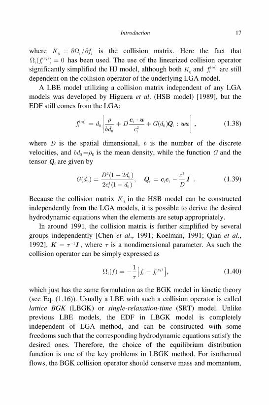
A LBE model utilizing a collision matrix independent of any LGA
models was developed by Higuera et al. (HSB model) [1989], but the
EDF still comes from the LGA:
( )0 02
0
:( )eq ii i
i
f d D G dbd c
ρ
⋅= + +
Qc u
uu , (1.38)
where D is the spatial dimensional, b is the number of the discrete
velocities, and bd0 =ρ0 is the mean density, while the function G and the
tensor Qi are given by
2 2
00 4
0
(1 2 )( ) ,
2 (1 )i i i
i
D d cG d
c d D
−= = −
−Q c c I . (1.39)
Because the collision matrix Kij in the HSB model can be constructed
independently from the LGA models, it is possible to derive the desired
hydrodynamic equations when the elements are setup appropriately.
In around 1991, the collision matrix is further simplified by several
groups independently [Chen et al., 1991; Koelman, 1991; Qian et al.,
1992], 1τ−=K I , where τ is a nondimensional parameter. As such the
collision operator can be simply expressed as
( )1( ) eq
i i if f fτ
Ω = − − , (1.40)
which just has the same formulation as the BGK model in kinetic theory
(see Eq. (1.16)). Usually a LBE with such a collision operator is called
lattice BGK (LBGK) or single-relaxation-time (SRT) model. Unlike
previous LBE models, the EDF in LBGK model is completely
independent of LGA method, and can be constructed with some
freedoms such that the corresponding hydrodynamic equations satisfy the
desired ones. Therefore, the choice of the equilibrium distribution
function is one of the key problems in LBGK method. For isothermal
flows, the BGK collision operator should conserve mass and momentum,

18 Lattice Boltzmann Method and Its Applications in Engineering
i.e.,
( ) ( ),eq eqi i i i i i
i i i i
f f f fρ ρ= = = =∑ ∑ ∑ ∑c cu . (1.41)
The use of the BGK collision operator enhances greatly the
computational efficiency of LBE, and makes the implementation of the
collision process much easier than other models. The LBGK model is
perhaps the most popular one in the LBE community.
1.3.3 From continuous Boltzmann equation to LBE
As shown above, LBE was originated from the LGA method. On the
other hand, it can show that LBE can also be derived from the continuous
Boltzmann equation. For simplicity and without loss of generality, we
take the isothermal LBGK model as an example. The starting point is the
Boltzmann equation with the BGK approximation,
( )
( ) ( ) ( )ξ
ξ ξ ξ ξ, , 1
, , , , , ,eq
c
f tf t f t f t
t τ
∂ + ⋅ ∇ = − − ∂
xx x x , (1.42)
where ( )eqf is the Maxwellian distribution function. The first step is to
discretize the velocity space of ξ into a finite set of velocities ic
without affecting the conservation laws. To do so, ( )eqf is first expanded
into a Taylor series in terms of the fluid velocity,
ξξ ξ2 2( )
2
2
/
(exp 1
(2 ) 2
)
2 2eq
Df
R
u
T RT RT T RTR
ρ
π
⋅⋅ = − + + −
uu. (1.43)
It should be born in mind that this expansion can only be used for low
Mach number flows, i.e. | |/ 1RTu . In order to obtain the correct
Navier-Stokes equations in the limit of low Mach number, the discrete
velocity set should be chosen so that the following quadratures of the
expanded EDF hold exactly
ξ ξ( ) ( )( ), 0 3k eq k eqi i i
i
f d w f k= ≤ ≤∑∫ cc (1.44)
where wi and ci are the weights and points of the numerical quadrature
rule. Based on the formulation of the expanded EDF given by Eq. (1.43),
it is natural to choose a Gaussian quadrature with at least fifth-order.

Introduction 19
Once the quadrature rule is chosen, we can define a discrete distribution
function, ( , ) ( , , )i i if t w f t=x x c , which satisfies the following equation
( )1 eqii i i i
c
ff f f
t τ
∂ + ⋅ ∇ = − − ∂c , (1.45)
where ( ) ( )( , ) ( , , )eq eqi i i if t w f t=x x c . Obviously, the fluid density and velocity
can be obtained from the discrete distribution function,
,i i i
i i
f fρ ρ= =∑ ∑u c . (1.46)
Integrating equation (1.45) from t to tt δ+ along the characteristic line
and assuming that the collision term is constant during this interval, we
can obtain
( )( , ) ( , ) ( , ) ( ,1
)eqi i t t i i if t f t f t f tδ δ
τ + + − = − − x c x x x , (1.47)
where /c tτ τ δ= is the dimensionless relaxation time. Clearly, this is just
the LBGK model.
1.4 Basic Models of LBE
In this section we will list some widely used LBE models for isothermal
flows, and then show how to derive macroscopic equations from LBGK
models using an asymptotical method. LBE models for thermal flows
will be detailed in one specific chapter.
1.4.1 LBGK models
The LBGK models are the most popular LBE method and have been
widely applied in variety of complex flows. Among the available models,
the group of DnQb (n-dimensional b-velocity) models proposed by Qian
et al. are the most representative ones [1992]. In DnQb, the discrete EDF
can be expressed as
2 2
( )
2 4 2
( )1
2 2
ieq ii i
s s s
uf
c c cω ρ
⋅ = + + −
⋅
uc c u, (1.48)

20 Lattice Boltzmann Method and Its Applications in Engineering
where ω i is the weight associated with the velocity ci , and the sound
speed cs is model dependent. In Tab. 1.1 several popular DnQb models
are presented (here the lattice speed c is assumed to be 1).
The lattice velocities of the DnQb models can form certain lattice
tensors with different ranks. The n-th rank lattice tensor is defined as
1 2 1 2... ...
n ni i i
i
L c c cα α α α α α= ∑ . (1.49)
Consequently, we have the 1st, 2
nd, 3
rd and 4
th rank lattice tensors as
, , ,
.
i i i i i i
i i i
i i i i
i
L c L c c L c c c
L c c c c
= = =
=
∑ ∑ ∑
∑
α α αβ α β αβγ α β γ
αβγζ α β γ ζ
(1.50)
A tensor of n-th rank is called isotropic if it is invariant with respect to
arbitrary orthogonal transformations (rotations and reflections). The most
general isotropic tensors up to 4th rank are provided by the following
theorem.
Table 1.1. Parameters of some DnQb models.
Model Lattice vector ic Weight iw 2sc
D1Q3 0,
±1
2/3,
1/6 1/3
D1Q5
0,
±1,
±2
6/12,
2/12,
1/12
1
D2Q7
(0,0),
(±1/2, ± 3 2 )
1/2,
1/12 1/4
D2Q9
(0,0),
(±1,0),(0, ±1),
(±1, ±1)
4/9,
1/9,
1/36
1/3
D3Q15
(0,0,0),
(±1,0,0), (0, ±1,0),(0,0, ±1),
(±1, ±1, ±1)
2/9,
1/9,
1/72
1/3
D3Q19
(0,0,0),
(±1,0,0), (0, ±1,0),(0,0, ±1),
(±1, ±1,0), (±1,0, ±1),(0, ±1, ±1)
1/3,
1/18,
1/36
1/3
Introduction 21
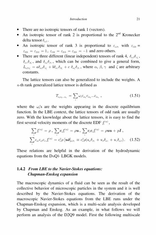
• There are no isotropic tensors of rank 1 (vectors).
• An isotropic tensor of rank 2 is proportional to the 2nd
Kronecker
delta tensor αβδ .
• An isotropic tensor of rank 3 is proportional to αβγε with 123ε =
231 312 1ε ε= = , 132 213 321 1ε ε ε= = = − and zero others.
• There are three different (linear independent) tensors of rank 4, αβ γζδ δ ,
αγ βζδ δ , and αζ βγδ δ , which can be combined to give a general form,
L a b cαβγζ αβ γζ αγ βζ αζ βγδ δ δ δ δ δ= + + , where α, β, γ and ζ are arbitrary
constants.
The lattice tensors can also be generalized to include the weights. A
n-th rank generalized lattice tensor is defined as
1 2 1 2... ...
n ni i i i
i
T c c cα α α α α αω= ∑ , (1.51)
where the ωi's are the weights appearing in the discrete equilibrium
function. In the LBE context, the lattice tensors of odd rank are usually
zero. With the knowledge about the lattice tensors, it is easy to find the
first several velocity moments of the discrete EDF ( )eqif ,
( )eqi
i
f ρ=∑ , ( )eqi i
i
f ρ=∑c u , ( )eqi i i
i
f pρ= +∑ c uuc I ,
δ( ) 2 2[ ] ( )eq
i i i i s s
i
f c c u uc uc cα β γ αβγ α βγ β αγ γ αβρ ρ δ δ δ= + +≡∑ u . (1.52)
These relations are helpful in the derivation of the hydrodynamic
equations from the DnQb LBGK models.
1.4.2 From LBE to the Navier-Stokes equations:
Chapman-Enskog expansion
The macroscopic dynamics of a fluid can be seen as the result of the
collective behavior of microscopic particles in the system and it is well
described by the Navier-Stokes equations. The derivation of the
macroscopic Navier-Stokes equations from the LBE runs under the
Chapman-Enskog expansion, which is a multi-scale analysis developed
by Chapman and Enskog. As an example, in what follows we will
perform an analysis of the D2Q9 model. First the following multiscale
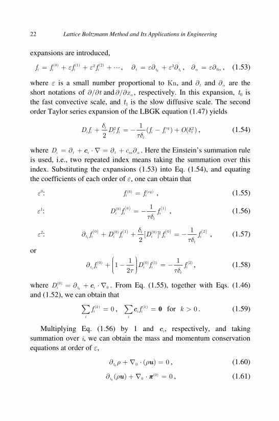
22 Lattice Boltzmann Method and Its Applications in Engineering
expansions are introduced,
(0) (1) (2)2i i i if f f fε ε= + + + ,
0 1
2t t tε ε∂ = ∂ + ∂ , 0α αε∂ = ∂ , (1.53)
where ε is a small number proportional to Kn, and t∂ and α∂ are the
short notations of / t∂ ∂ and / xα∂ ∂ , respectively. In this expansion, t0 is
the fast convective scale, and t1 is the slow diffusive scale. The second
order Taylor series expansion of the LBGK equation (1.47) yields
2 21( ) ( )
2eq
i i i i i i tt
t
D f D f f f O δτδ
δ+ = − − + , (1.54)
where i t i t iD c α α= ∂ + ⋅ ∇ = ∂ + ∂c . Here the Einstein’s summation rule
is used, i.e., two repeated index means taking the summation over this
index. Substituting the expansions (1.53) into Eq. (1.54), and equating
the coefficients of each order of ε, one can obtain that
ε0: (0) ( )eqi if f= , (1.55)
ε1: ( ) ( )0 1(0) 1
t
i i iD f fτδ
= − , (1.56)
ε2: ( ) ( ) ( ) ( )1
0 1 0 2(0) (0) 2 1[ ]
2t i
ti i i i i
t
f D f D f fδ
δ
τ∂ + + = − , (1.57)
or
1
(0) (0) (1) (2)1 11
2t i i i i
t
f D f fτ τδ
∂ + − = − , (1.58)
where 0
(0)0i t iD = ∂ + ⋅ ∇c . From Eq. (1.55), together with Eqs. (1.46)
and (1.52), we can obtain that
( ) 0ki
i
f =∑ , ( )ki i
i
f =∑ 0c for 0k > . (1.59)
Multiplying Eq. (1.56) by 1 and ci , respectively, and taking
summation over i, we can obtain the mass and momentum conservation
equations at order of ε,
0 0 ( ) 0t ρ ρ⋅∂ + ∇ =u , (1.60)
π0 0
(0)( ) 0t ρ∂ + ∇ ⋅ =u , (1.61)

Introduction 23
where (0) (0)i iic c f u u pα β α β αβαβπ ρ δ= = +∑ is the zeroth-order momentum
flux tensor, with 2sp c ρ= . Here the following properties of the generalized
lattice tensors of the D2Q9 model have been used:
0i i i i i i
i i
c c c cα α β γω ω= =∑ ∑ , 2i i i s
i
c c cα β αβω δ=∑ ,
4i i i i i s
i
c c c c cα β γ θ αβγθω = ∆∑ , (1.62)
where αβγζ αβ γζ αγ βζ αζ βγδ δ δ δ δ δ∆ = + + . Equations (1.60) and (1.61) are
the Euler equations, just the same as those from the continuous
Boltzmann equation in kinetic theory.
Similarly, the zeroth and first order moments of Eq. (1.58) leads to
the conservation equations at order of ε2,
1
0t ρ∂ = , (1.63)
1
12
π1
(1)0( ) 0t
τρ
− ∂
⋅∇+ =u , (1.64)
where (1) (1)i i iic c fα βαβπ = ∑ . In order to evaluate (1)
αβπ , we multiply Eq. (1.56)
by i ic cα β and take summation over i:
( )0
0
0 0
0
(1) (0) (0)0
2
20
20 0
20 0 0
20 0
1=
=
( )
( ) ( )
i i i t i i i i i i
i i it
t s
s
s t t
t s
s
c c f c c f c c c f
u u c
c u u u
c u u u p
u u p c u u
c u u
α β α β γ α β γ
α β αβ
γ α βγ β αγ γ αβ
γ γ αβ β α α
α β β α β β α
α β β α
τδ
ρ ρδ
ρ δ δ δ
ρ ρ δ ρ
ρ ρ
ρ
− ∂ + ∂
∂ ++ ∂ + +
∂ + ∂ + ∂ + ∂ + ∂ + ∂ + ∂ + ∂
=
=
∂ + ∂
∑ ∑ ∑
0
2 30 0
( )
( ) ,s
u u u
c u u O M
γ α β γ
α β β α
ρ
ρ
− ∂ = ∂ + ∂ +
(1.65)
where M is the Mach number. Here the equations on the first order of ε ,
(1.60) and (1.61) have been used to evaluate the time derivatives.
Specifically, the following relations have been applied:
0 0 ( )t uβ βρρ∂ ∂−= , (1.66)
0
(0)0 0 0( ) ( )t u p u uαα β α βα ββρ π ρ= − ∂−∂ = −∂ ∂ , (1.67)
0 0 0t u p u uα α β β αρρ∂ = ∂ ∂− − , (1.68)

24 Lattice Boltzmann Method and Its Applications in Engineering
where the last equation is derived from the first two equations. Equation
(1.65) gives then that (1)0 0( )p t u uα β β ααβπ τ δ= − ∂ + ∂ after neglecting the
terms of O(M 3).
Combining the mass and momentum conservation equations on both
the ε and ε2 scales, we can get the hydrodynamic equations correspond-
ing to the D2Q9 model:
( ) 0tρ ρ∂ + ∇ ⋅ =u , (1.69)
( )( )( ) Tp
t
ρρ ρν
∂ + ∇ = −∇ + ∇ ⋅ ∇ + ∇ ∂u
uu u u , (1.70)
where ν is kinematic viscosity given by
2 1
2s tcν τ δ = −
, (1.71)
and / 3sc c= for the D2Q9 model. In small Mach number limit, the
density variation can be negligible. Thus one can further obtain the
incompressible Navier-Stokes equations
0 ∇ ⋅ =u , (1.72)
21
pt
νρ
∂+ ⋅ ∇ = − ∇ + ∇
∂u
u u u . (1.73)
It is noted that low Mach number assumption has been employed in both
the expansion of the discrete EDF from the Maxwellian distribution
function and the derivation given above. As such, the LBGK models are
only suitable for low speed flows in principle. On the other hand, it is
known that the density variation of a flow is proportional to the square of
the Mach number, which means that the LBGK method is actually an
artificial compressibility method for the incompressible Navier-Stokes
equations. Therefore, besides the temporal and spatial discretization
errors, LBGK method also suffers from an additional error from the
compressibility when applied to incompressible flows. Several
incompressible LBGK models have been developed to overcome the
compressibility error from different viewpoints [Zou et al., 1995; He and
Luo, 1997; Chen and Ohashi, 1997; Guo et al., 2000].

Introduction 25
Now we discuss the accuracy of the LBGK models. First it is noted
that the LBGK equation (1.47) is a first-order finite-difference scheme
for the discrete velocity Boltzmann equation (1.45). If we apply the
Chapman-Enskog analysis to the Eq. (1.45) directly, we can also derive
the isothermal or athermal Navier-stokes equations (1.70), but with a
kinematic viscosity 2 2s c tsc cν τ δτ= = which contains no temporal and
spatial discretization errors. In the above analysis, however, the
expansion of the LBGK equation (1.47) was truncated up to O( 2tδ ) and
O( 2xδ ), which means that LBGK method can be viewed as a second-order
scheme for the compressible Navier-Stokes equations after absorbing the
numerical viscosity 2 /2tn scν δ= , which comes from the term 2 2( /2)t i iD fδ
in Eq. (1.54), into the physical one. This is an appealing feature of the
LBGK method for complex flows. Also, because the underlying lattices
of the LBGK models posses better rotational symmetry than classical
second-order finite-difference/finite-volume schemes, LBGK and other
LBE models may yield more accurate results than classical CFD methods
with the same temporal and spatial accuracies. Actually, some
comparative studies indicate that the results of LBE are even comparable
to spectral methods for turbulent flows [Martinez et al., 1994].
1.4.3 LBE models with multiple relaxation times
Like the BGK model in kinetic theory, the LBGK model uses a
relaxation process with a single relaxation time to characterize the
collision effects, which means that all of the modes relax to their
equilibria with the same rate. However, physically, these rates should be
different during the collision process. In order to overcome this
limitation, a collision matrix with different eigenvalues or multiple
relaxation times can be used. Actually, such models were proposed by
d'Humèriers almost at the same time when the LBGK method was
developed [d'Humières, 1992]. Such MRT-LBE models have been
attracting more and more attentions recently due to some inherent
advantages [Lallemand and Luo, 2000].
The LBE with a MRT collision operator can be expressed as,
( )( , ) ( , ) , 0 1eqi i t t i ij j j
j
f t f t f f i b + + − = − Λ − = − ∑x c x ∼δ δ , (1.74)

26 Lattice Boltzmann Method and Its Applications in Engineering
or
Λ ( )( , ) ( , ) ( )eqi t t t tδ δ+ + − = − −f x c f x f f , (1.75)
where b is the number of discrete velocities, and ΛΛΛΛ is the collision matrix.
Equation (1.74) or (1.75) describes the evolution of the population
0 11( , , , )Tbf f f −= f in the velocity space V. On the other hand, the
evolution process can also be described in a moment space M. To see
how this is realized, we first define b moments based on f,
k km φ= ⋅f , k = 0 ∼ b −1, (1.76)
where kφ is a vector with b elements, each of which is a polynomial of
the discrete velocities. These b vectors are independent and thus form a
basis of the velocity space. The relation between the moments and the
distribution functions can also be expressed in a concise form,
0 1 1( , , , )Tbm m m −= = m Mf , (1.77)
where the invertible transformation matrix M is composed of the vectors
kφ . The space where the moments take values is just the moment space.
From Eq. (1.75), we can obtain the moment evolution equation as,
( )( , ) ( , ) ( )eqi t tt tδ δ+ + − = − −m x c m x S m m , (1.78)
where Λ 1−=S M M is usually a diagonal matrix, i.e. S = diag (s0, s1, …,
sb−1), and ( ) ( )eq eq=m Mf is the equilibria in the moment space.
In practical applications, however, the MRT-LBE usually combines
the evolutions in the velocity space and moment space. That is, the
collision step is executed in the moment space while the streaming step is
still performed in the velocity space just like the LBGK method.
Therefore, the basic flowchart of a MRT-LBE model can be described as
follows,
• Transforming the distribution functions f to moments m according to
Eq. (1.77);
• Colliding in moment space: ( )( )eq′ = − −m m S m m ;
• Transforming the post-collision moments m' back to the post-
collision distribution function: 1−′ ′=f M m ;
• Streaming in velocity space: ( , ) ( , )i i t t if t f tδ δ ′+ + =x c x .

Introduction 27
Therefore, the evolution of the MRT-LBE can be effectively expressed
as
1 ( )( , ) ( , ) ( )eqi t tt tδ δ −+ + − = − −f x c f x M S m m . (1.79)
In MRT-LBE, the relaxation rates si, or the relaxation times τi = 1/si can
be tuned with some freedom. This means that these parameters can be
optimized to enhance the performance of the algorithm [Lallemand and
Luo, 2000]. It is also noted that as si =1/τ, the MRT-LBE reduces to the
LBGK models. Nonetheless, the involvement of the transforms between
the velocity and moment spaces will increase some computational costs.
However, the increase is not significant because M is usually an
orthogonal matrix. Some numerical tests demonstrate that the increase in
time is within 20% [d'Humières et al., 2002].
The transformation matrix M, or the base vectors kφ , can be
constructed from the polynomials m n lix iy izc c c (m, n, l ≥ 0) through the
Gram-Schmidt orthogonalization [Bouzidi et al., 2001]. Generally, the
basis includes the following vectors corresponding to the mass and
momentum:
0
1 2
(1 , 1 , , 1)
( , , , ) , 1 , 2 , , .
Tb
bT
bc c c Dα α α α α
= ≡
= =
1
φ
φ
(1.80)
Another key point of the MRT-LBE model is the equilibria in moment
space. In principle m(eq) can be constructed with some freedoms. But a
more convenient way is to compute them from the discrete EDFs fi(eq)
of
the DnQb models once the transformation matrix M is determined.
Several 2D and 3D MRT-LBE models are listed below. For simplicity,
we assume that c = 1.0 in all cases, otherwise the base vectors can be
normalized by c and the results are similar.
(1) Standard D2Q9 model
The lattice is the same as the D2Q9 LBGK model, i.e, a two-dimensional
square lattice. The corresponding moments are
( ), , , , , , , ,T
x x y y xx xye j q j q p pρ ε=m ,

28 Lattice Boltzmann Method and Its Applications in Engineering
while the equilibria in the moment space are
( )( ) 2 2 2 21, 2 3 , , , , , , ,T
eqx x y y x y x yu u u u u u u u u uρ α β= − + + − − −m ,
where α and β are two free parameters, and when α = 1 and β = −3, the
equilibria are consistent with those of the D2Q9 LBGK model. The
transformation matrix is
1 1 1 1 1 1 1 1 14 1 1 1 1 2 2 2 24 2 2 2 2 1 1 1 10 1 0 1 0 1 1 1 10 2 0 2 0 1 1 1 10 0 1 0 1 1 1 1 10 0 2 0 2 1 1 1 10 1 1 1 1 0 0 0 00 0 0 0 0 1 1 1 1
− − − − − − − − − − − − − − −= − − − − − − − − − −
M .
The relaxation rates corresponding to the moments are
(0 , , , 0 , , 0 , , , )e q qs s s s s sε ν ν=S ,
and the kinematic viscosity and bulk viscosity are related to the
relaxation rates se and sν,
2 21 1 1 1,
2 2s t s t
e
c cs sν
ν δ ζ δ = − = −
,
where 2 1/3sc = .
(2) Rectangular D2Q9 model
An advantage of MRT-LBE is that a nonstandard mesh can be used as
the underlying lattice due to the freedoms in choosing the equilibria and
the relaxation times. For example, a D2Q9 MRT-LBE model using a
rectangular lattice has been developed. The lattice vectors are given by
0 1 0 1 0 1 1 1 1
0 0 0a a a a a a
− − − = − − − c ,

Introduction 29
where /y xa δ δ= is the ratio of the lattice spacing and here δx is set to be
unity. The nine moments are
( ), , , , , , , 3 ,T
x x y y xx xye j q j q p pρ ε=m ,
and the corresponding equilibria are given by
( )
( ) 2 2 2 2 21 4
2 2 2 2 2 24
41
1 , 2(3 ) 3 , , 1 3 , , ( 4 2 ,
, , (
)/
/2 /3 2 )/3 + , ,
eqs x x
T
y y s x y x y
c r u u u u u r a
u u r r c a a u u u uaa
ρ α β γ
γ
= − + + − −− − −
m
where cs , α, β, and γ are free parameters. The transformation matrix is
1 2 3 2 3 1 1 1 1
4 5 6 5 6 4 4 4 4
1 1 1 1 1 1 1 1 1
2
4 2 2 2 2 1 1 1 1
0 1 0 1 0 1 1 1 1
0 2 0 2 0 1 1 1 1
0 0 0
0 0 2 0 2
2
0 0 0 0 0 1 1 1 1
r r r r r r r r r
a a a a a a
a a a a a a
r r r r r r r r r
− − − − − − − − − − −= − − − − − − − − −
M ,
where 21 1r a= + , 2
2 1 2r a= − , 23 2r a= − + , 2
4 1r a= − + , 25=2+r a ,
and 26 1 2r a= − − . The relaxation rates are similar to those of the
standard D2Q9 model,
(0, , , 0, , 0, , , )e q qs s s s s sε ν ν=S .
The shear and bulk viscosities are
2 24 1 1 7 3 12 1 1
,6 2 12 2
st t
e
a c
s sν
γ γν δ ζ δ
+ + + − = − = − .
As expected, if a = 1, 2 1/3sc = , and γ = −2, this rectangular model
reduces to the standard D2Q9 model. It should be noted that the
corresponding rectangular D2Q9 LBGK model does not exist.

30 Lattice Boltzmann Method and Its Applications in Engineering
(3) D3Q13 model
D3Q13 MRT-LBE model uses the following discrete velocities,
0 1 1 1 1 1 1 0 0
0 1 1 1 1
0 0 0 1
0 0 1 1
0 0 1 1 1 1
1 1 1 1
0 0
1 1 0 0 1
− −−
−
− − = − − − − − −
c .
The corresponding moments are
( ), , , , , 3 , , , , , , ,T
x y z xx ww xy yz zx x y zj j j e p p p p p t t tρ=m ,
with the following equilibrium moments,
(
)
3 13( ) 2 2 2 2 2 2
2 21, , , , (13 8) , 3 , ,
, , , 0, 0, 0 .
eqx y z s x y z
T
x y y z z x
u u u c u u u u u
u u u u u u
ρ= − + − −m
The corresponding transformation matrix is
1 1 1 1 1 1 1 1 1 1 1 1 1
0 1 1 1 1 0 0 1 1 1 1 0 0
0 1 1 0 0 1 1 1 1 0 0 1 1
0 0 0 1 1 1 1 0 0 1 1 1 1
12 1 1 1 1 1 1 1 1 1 1 1 1
0 1 1 1 1 2 2 1 1 1 1 2 2
0 1 1 1 1 0 0 1 1 1 1 0 0
0 1 1 0 0 0 0 1 1 0 0 0 0
0 0 0 0 0 1 1 0 0 0 0 1 1
0 0 0 1 1 0 0 0 0 1 1 0 0
0 1 1 1 1 0 0 1 1 1 1 0 0
0 1 1 0 0 1 1 1 1 0 0 1 1
0 0 0 1 1
− − − −− − − −
− − − −−
− − − −− − − −=
− −− −
− −− − − −
− − − −−
M
1 1 0 0 1 1 1 1
− − −
,
and the relaxation rates are
(0, 0, 0, 0, , , , , , , , , )e t t ts s s s s s s s sν ν ν ν ν′ ′ ′=S ,
while the shear and bulk viscosities are ( 2 1/3sc = )
21 1 1 1 1 1 2 3 1 1
,4 2 2 2 3 2
st t t
e
c
s s sν ν
ν δ δ ζ δ − = − = − = − ′
.

Introduction 31
(4) D3Q15 model
This model shares the same discrete velocities as the D3Q15 LBGK
model. The fifteen moments are
( ), , , , , , , , , 3 , , , , ,T
x x y y z z xx ww xy yz zx xyze j q j q j q p p p p p tρ ε=m ,
with the corresponding equilibria,
( ) 2
2 2 2 2
7 7 71, 1, 1, , , , , , ,
3 3 3
3 , , , , , 0 .
eqx x y y z z
T
x y z x y y z z x
u u u u u u u
u u u u u u u u u u
ρ= − − − − −
− −
m
The transformation matrix is given as follows,
1 1 1 1 1 1 1 1 1 1 1 1 1 1 12 1 1 1 1 1 1 1 1 1 1 1 1 1 1
16 4 4 4 4 4 4 1 1 1 1 1 1 1 10 1 1 0 0 0 0 1 1 1 1 1 1 1 10 4 4 0 0 0 0 1 1 1 1 1 1 1 10 0 0 1 1 0 0 1 1 1 1 1 1 1 10 0 0 4 4 0 0 1 1 1 1 1 1 1 10 0 0 0 0 1 1 1 1 1 1 1 1 1 10 0 0 0 0 4 4 1 1 1 1 1 1 1 10 2 2 1 1 1 1 0 0 0 0 0 0 0 0
− − − − − − −− − − − − −
− − − − −− − − − −
− − − − −− − − − −
− − − − −=− − − − −
− − − −
M
0 0 0 1 1 1 1 0 0 0 0 0 0 0 00 0 0 0 0 0 0 1 1 1 1 1 1 1 10 0 0 0 0 0 0 1 1 1 1 1 1 1 10 0 0 0 0 0 0 1 1 1 1 1 1 1 10 0 0 0 0 0 0 1 1 1 1 1 1 1 1
− − − − − − − − − − − − − − − − − −
.
The relaxation rates are set as follows,
(0, , , 0, , 0, , 0, , , , , , , )e q q q ts s s s s s s s s s s=S ε ν ν ν ν ν ,
which are related to the viscosities as follows,
,1 1 1 2 1 1
3 2 9 2t t
es sν
ν δ ζ δ = − = −
.

32 Lattice Boltzmann Method and Its Applications in Engineering
(5) D3Q19 model
The discrete velocity set of the D3Q19 MRT model is the same as that of
the LBGK model. The corresponding moments are
( ), , , , , , , , , 3 , 3 , , , , , , , ,T
x x y y z z xx xx ww ww xy yz zx x y ze j q j q j q p p p p p t t tρ ε π π=m ,
while the corresponding equilibrium moments are
( ) 2 2
( ) ( )2 2 2 2
2 2 21, 11 19 , , , , , , , ,
3 3 3
3 , , , , , , , 0, 0, 0 ,
eqx x y y z z
Teq eqxx ww
x y z x y y z z x
m u u u u u u u u
p pu u u u u u u u u u
= − + + − − −− −
ρ α β
γ γ
ρ ρ
where α, β, and γ are free parameters. As α = 3, β = −11/2, and γ = −1/2,
the equilibria reduce to those of the D3Q19 LBGK model. The
transformation matrix of this model is
.
The relaxation rates of this model are
(0, , , 0, , 0, , 0, , , , , , , , , , , )e q q q t t ts s s s s s s s s s s s s s sε ν π ν π ν ν ν=S ,
while the shear and bulk viscosities as
,1 1 1 2 1 1
3 2 9 2t t
es sν
ν δ ζ δ = − = −
.

Introduction 33
It can be shown that with the equilibrium moments described above,
the Navier-Stokes equations can be obtained either by the Chapman-
Enskog expansion method [d'Humières, 1992; d'Humières et al., 2002]
or a linear analysis [Lallemand and Luo, 2000].
1.5 Summary
In this chapter we have presented an overview of the LBE method. It can
be seen that the LBE is a novel approach for fluid dynamics, quite
different from the classical CFD techniques that are based on the solution
of Navier-Stokes equations. Firstly, although LBE aims to solve
continuum flows at macroscopic scales, it is developed based on
microscopic models (LGA) or kinetic theory (Boltzmann equation). This
feature suggests that the LBE has the potential to model nonequilibrium
flows which cannot be described by the Navier-Stokes equations.
Secondly, the kinetic nature of LBE makes it suitable for describing the
internal interactions among fluid particles and those between the fluid
and external environment, and this brings great advantages in simulating
complex flows such as multi-component/phase flows and flows in porous
media. Finally, the clear evolution picture of LBE makes it quite easy to
code; Particularly, the collision process involves only local computations
and the streaming process can be realized by simple index shift
operations, which makes LBE well suited for massive parallel computers.
These distinctive features have made LBE an attractive numerical
tool for modeling and simulating complicated fluid flows and associated
phenomena. Actually, LBE can find its applications in simulation of
laminar and turbulent flows, interfacial dynamics of multiphase flows,
flows in porous media, particulate and suspension systems, bio-fluid
mechanics, electro-kinetic flows, magneto-hydrodynamics, quantum and
relativistic flows, nano/micro fluidics, and multiscale flows. The
developments of LBE at different stages have been summarized in
several excellent review papers [Benzi et al., 1992; Chen and Doolen,
1998; Yu et al., 2003; Aidun and Clausen, 2010], and a number of books
on both general LBE methods [Wolf-Gladrow, 2000; Succi, 2001] and
specific topics [Sukop and Thorne, 2006; Zhou, 2004] are also available.

34 Lattice Boltzmann Method and Its Applications in Engineering
The past two decades have witnessed the rapid development and great
success of LBE in fundamental theory and applications in a variety of
related areas, and nowadays the research in this field is still very active
and exciting. The LBE has been becoming a topic of great interest in
many international conferences, and even two specific conferences on
this subject, DSFD (International Conference on the Discrete Simulation
of Fluid Dynamics) and ICMMES (International Conference for
Mesoscopic Methods in Engineering and Science), have been established.

35
Chapter 2
Initial and Boundary Conditions for
Lattice Boltzmann Method
Initial and boundary conditions play an important role in fluid dynamics
since they are essential in the determination of the solution of the flow.
Generally, these conditions are specified in terms of the fluid variables
such as velocity, pressure, and temperature. However, the primitive
variable in LBE is the discrete distribution function. The fluid density
and velocity (and temperature in thermal flows) can be determined
uniquely by the distribution function, but not vice versa. Therefore, it is
critical for LBE to find a way to transform the initial and boundary
conditions from the fluid variables to those for the distribution functions.
Some studies have revealed that these conditions do have significant
influences on the accuracy, stability, and convergence of LBE. So, the
treatments of initial and boundary conditions are a fundamental topic in
the study and applications of LBE. In this chapter, we will present some
useful rules for realizing these conditions in LBE. We will focus on
isothermal cases unless mentioned otherwise.
2.1 Initial Conditions
2.1.1 Equilibrium scheme
The equilibrium scheme is a widely used method for imposing initial
conditions in LBE. In this scheme, the distribution functions are
initialized as the equilibria directly,
( )0 0 0( ) ( , ), 0 1eq
i if t f i bρ= = −u ∼ , (2.1)

36 Lattice Boltzmann Method and Its Applications in Engineering
where ρ0 and u0 are the initial values of density and velocity at time t0. In
many problems, only the velocity is initialized and the density (or
pressure) is unknown. In such case, the density must be determined first
from the velocity field in a compatible manner. For instance, the initial
pressure p0 can be obtained by solving a Poisson equation for
incompressible flows, and then the density can be initialized as
0 2s
p p
cρ ρ
−= + , (2.2)
where ρ and p are the average density and pressure, respectively.
For steady or quasi-steady flows, the final results are independent of
initial conditions, and the equilibrium scheme will work well. But for
unsteady or strong nonlinear flows which are very sensitive to initial
conditions, this scheme may lead to large errors due to the initial layers
in the discrete distribution functions. In such cases, more accurate initial
schemes should be adopted.
2.1.2 Non-equilibrium scheme
In order to increase the approximation accuracy to fi(t0), we can introduce
some corrections from the non-equilibrium part of the distribution
function, ( ) ( )neq eqi i if f f= − . This technique was first proposed by Skordos
[1993]. The key point of such schemes is how to obtain the non-
equilibrium part from initial conditions.
We first consider the LBGK models. The LBGK equation gives that
( )( , ) ( , ) ( , )neqi i i t t if t f t f tτ δ δ = − + + − x x c x . (2.3)
The Taylor expansion of the right hand side gives that
( ) 2( )neqi t i i tf D f Oτδ δ= − + , (2.4)
where i t iD = ∂ + ⋅ ∇c . On the other hand, the distribution function can
be expanded into a series following the Chapman-Enskog method,
( ) (1) (2)2eqi i i if f f fεε= + + + , (2.5)

Initial and Boundary Conditions for Lattice Boltzmann Method 37
where the expansion parameter ε is proportional to the Knudsen number
which is very small for continuum flows. Therefore, the non-equilibrium
distribution function can be approximated as
( ) ( )
( ) ( )eq eq
neq ei
q i ii t i i t iD
f ff D f Dτδ τ
ρρδ
∂ ∂ − = − + ⋅ ∂ ∂
≈j
j, (2.6)
where j =ρu. In the above equation ( )/eqif ρ∂ ∂ and ( )/eq
if∂ ∂j can be
evaluated exactly from the expressions of ( )eqif . For example, the EDF of
the DnQb models gives that
2)
2
( 2
4
( )1
2 2
ieqi
i
s sc c
fω
ρ
∂
∂
⋅ = − +
c u u, (2.7)
2 4
( ) ( )i iii
s
qi
s
ef
c cω
⋅− = +
∂
∂
c u cc
j
u. (2.8)
The temporal and spatial derivatives in Eq. (2.6) should be evaluated
numerically, and the two temporal derivatives can be converted into
spatial gradients first following the conservation equations. If the
hydrodynamic equations at the t0 scale in the Chapman-Enskog
expansion (i.e. the Euler equations) are used, we can obtain that
( )i iD ρ ρ ρ= − ⋅ ∇ − ∇ ⋅c u u , ( )i iD p= −∇ + − ⋅ ∇ − ∇ ⋅j c u j j u . (2.9)
Alternatively, we can use the Navier-Stokes equations to evaluate the
temporal derivatives, which give that
( ) ,
( ) ,
i i
i i
D
D p
ρ ρ ρ= − ⋅ ∇ + ∇ ⋅
= −∇ + ∇ ⋅ + − ⋅ ∇ − ∇ ⋅
c u u
j c u j j uτ
(2.10)
where τ is the stress tensor.
Substituting the above results into Eq. (2.6), one can obtain an
explicit approximation to the non-equilibrium distribution function,
which is quite complicated. In order to simplify the expressions, one can
ignore terms of second and high-order of M (Mach number). For
example, the final formulation of Eq. (2.6) can be expressed as
( )
2
1:neq
i t i i i
s
fc
= − ∇ − ∇ ⋅ c c u uρτδ ω . (2.11)

38 Lattice Boltzmann Method and Its Applications in Engineering
Guo et al. [2003] made a further simplification by noticing that 2(1 ) ( )O Mρ ρ δρ ρ= + = + for nearly incompressible flows,
( )
2:neq
i t i i i
s
fc
τδ ωρ
= − ∇c c u . (2.12)
This result is consistent with the mass and momentum conservation
constraints for incompressible flows,
( ) ( )0, 0neq neqi t i i
i i
f fτδ ρ ∇ ⋅= − = =∑ ∑u c . (2.13)
The above non-equilibrium schemes are designed for LBGK models,
and they can also be extended to MRT-LBE models. For instance,
Lallemand and Luo [2000] suggested correcting the initial moments
using the non-equilibria ones in moment space first, and then transform
back to the velocity to obtain the initial distribution functions:
( ) 1 ( ) 1 ( )ˆ= =eq eqt t
neq − −− ∂ − ∂S MC f S Cm mα α α αδ δ , ( ) 1 ( )neq neq−=f M m , (2.14)
where ( )0 0 1,, , , bdiag c c cα α α α−=C and 1ˆα α
−=C MC M .
2.1.3 Iterative method
In order to obtain consistent initial distribution functions from a given
velocity field, some researchers suggested solving a Poisson equation
using a LBE, which can provide both the desired pressure (or density)
and the distribution functions [Caiazzo, 2005; Mei et al., 2006]. For the
LBGK equation,
( )( )1( , ) ( , ) ( , ) ( , ), ( , )eqi i t t i i if t f t f t f t tδ δ ρ
τ + + − − −
x c x x x u x , (2.15)
the procedure of iterative initialization method is as follows,
(a) Collision:
( )( )0
1( , ) ( , ) ( , ) ( , ),eqi i i if t f t f t f tρ
τ ′ = − −
x x x x u .
(b) Streaming:
( , ) ( , )i i t t if t f tδ δ ′+ + =x c x .

Initial and Boundary Conditions for Lattice Boltzmann Method 39
(c) Calculating the predicted initial density:
( , ) ( , )t i t
i
t f tρ δ δ+ = +∑ xx .
(d) If ρ converges to its steady state ρ0, the iteration will end, and
the initial distribution functions as well as the density are set to
be 0( , ) ( , )i i tf t f t δ= +x x and 0 0( , )tρ ρ=x ( , )ttρ δ≡ +x , respec-
tively; otherwise, go to (a) for next iteration.
Note that in the above iterative procedure we have used the notation
with a tilde to distinguish the variables from the physical ones.
Meanwhile, in the EDF ( )eqif , the velocity always takes the initial value
during the pseudo time evolution, and only the density ρ acts as a
conservative variable. Actually, the iterative procedure corresponds to
the following modified LBGK equation,
( )( )0
1( , ) ( , ) ( , ) ( , ),eqi i t t i i if t f t f t f tδ δ ρ
τ + + − = −
x c x x x u , (2.16)
with the constraint that
( )( )0,eq
i i
i i
f fρ ρ= =∑ ∑ u . (2.17)
One can show that the hydrodynamic equation derived from this LBGK
equation via the Chapman-Enskog method is
2 20 0 02
( ) : ( )s
s
ct c
ρ νρ ρ ρ
∂ + ∇ ⋅ = ∇ + ∇∇ ∂u u u
. (2.18)
If the initial velocity field is incompressible, i.e., 0 0∇ ⋅ =u , at steady
state the leading order of the above equation is
20 0( )P =∇ ⋅−∇ ⋅ ∇u u , (2.19)
where 2sP c δρ= is the dynamic pressure. This means that the above
iterative procedure leads to a consistent initialized pressure field and the
distribution functions as well.
The iterative procedure can also be applied to MRT-LBE models with
some slight modifications [Mei et al., 2006]. The procedure is the same

40 Lattice Boltzmann Method and Its Applications in Engineering
as that for the LBGK model except that the collision is carried out in the
moment space, i.e., the collision step (a) is replaced by the following one:
(a') Collision:
( )( )0( , ) ( , ) ( , ) ( , ),eq
k k k k kt t s t tρ ′ = − − m x m x m x m x u ,
1,( ( , ))t t−′ = ′x m xf M .
Note that the momentum j is not a conservative variable and the
corresponding relaxation rate sj is nonzero. The corresponding hydro-
dynamic equation is the same as Eq. (2.18) except that the kinematic
viscosity appearing on the right hand side is now replaced by a
diffusivity 2( 0.5)s j tD c τ δ= − where τj =1/sj . Because the relaxation time
τj can be adjusted independently from that for the kinematic viscosity,
the iteration can achieve a faster convergence than that for the LBGK
models. This feature is particularly useful for high Reynolds number
flows where the viscosity is small.
2.2 Boundary Conditions for Flat Walls
Similar to initial conditions, the distribution functions at a boundary
should also be constructed to reflect specified boundary conditions for
fluid variables (pressure, velocity, and temperature). A variety of
boundary schemes have been introduced for LBE. According to
methodology employed, boundary conditions in LBE can be classified
into heuristic schemes, hydrodynamic schemes, and interpolation/
extrapolation schemes. We first present some boundary schemes for flat
boundaries.
2.2.1 Heuristic schemes
Heuristic or phenomenological schemes are designed based on the
dynamics of fluid particles as they encounter a wall. Several such
schemes are sketched in Fig. 2.1 for a flat wall. The bounce-back scheme
is the most widely used rule for stationary no-slip walls. This scheme
assumes that a particle just reverses its velocity after colliding with the

Initial and Boundary Conditions for Lattice Boltzmann Method 41
wall, which means that the post-collision distribution function at a
boundary node xb is
ı ( , ) ( , )b i ff t f t′ ′=x x , (2.20)
where ı i= −c c with ci pointing to the fluid, xb is a node located on the
wall, and f b i tδ= − cx x is the neighboring fluid node. Based on the
collision-streaming process, the bounce-back scheme can also be
expressed in alternative formulations,
ı ( , ) ( , )f t i ff t f tδ ′+ =x x , (2.21)
or
ı ( , ) ( , )f t i bf t f t tδ δ+ = +x x . (2.22)
Particularly, the formulation given by Eq. (2.21) has nothing to do with
boundary nodes and the computation is completely local, and therefore is
Fig. 2.1. Sketch of several heuristic schemes.
ic
ıc
bx
fx
Standard bounce-back
ic
ıc
bx
fx
Modified bounce-back
ic
ıc
bx
fx
Half-way bounce-back
ic
ıc
bx
fx
Specular-reflection
5
1
8
2 6
3
7 4
n

42 Lattice Boltzmann Method and Its Applications in Engineering
widely used in practical applications. For example, for the D2Q9 model
the unknown distribution functions in the directions 2, 5, and 6 can be
easily obtained as (see Fig. 2.1)
42( , ) ( , )f t ff t f tδ ′+ =x x , 75( , ) ( , )f t ff t f tδ ′+ =x x ,
86( , ) ( , )f t ff t f tδ ′+ =x x . (2.23)
It is noted that in the standard bounce-back scheme the collision
process is not carried out on the boundary nodes. If the collision is also
imposed on the boundary, the method is called modified bounce-back
scheme, which specifies the unknown pre-collision distributions at the
boundary nodes as follows,
ı ( , ) ( , )b i bf t f t=x x . (2.24)
Then the fluid density and velocity at the boundary nodes can be
calculated from the distribution functions, and the collision step can be
executed. The modified bounce-back scheme for the D2Q9 model can be
expressed as
42( , ) ( , )bf t f t= bx x , 75( , ) ( , )bf t f t= bx x , 86( , ) ( , )bf t f t= bx x . (2.25)
Another modification of the standard bounce-back scheme is the half-
way bounce-back scheme, whose formulation is totally identical to the
standard one except that the wall is placed at the middle of the link, (xb+
xf) /2. The physical picture of this scheme is clear: The post-collision
particles with velocity ci at node xf will arrive at the wall after time δt/2,
and are then reflected back to xf with a reversed velocity ıc after another
δt/2, and so ı ( , ) ( , )f t i ff t f tδ ′+ =x x , which is the same as the standard
bounce-back scheme. This also implies that the standard bounce-back
scheme does not exhibit such a physical picture. Actually, some studies
have shown that the half-way bounce-back scheme is of second-order
accuracy, while the standard one is only of first order [He et al., 1997].
Similar to the half-way bounce-back scheme, the modified bounce-back
scheme is also of second-order accuracy.
It is clear that in the bounce-back schemes, the momentum of a
particle is just reversed before and after it hits the wall, which means that
the macroscopic velocity at the wall is zero. Therefore, these bounce-back

Initial and Boundary Conditions for Lattice Boltzmann Method 43
schemes work for stationary walls. As the wall moves with a velocity uw,
the schemes should be modified to include the contribution of the
wall motion. For example, Ladd has suggested a revised half-way
bounce-scheme,
ı 2( , ) ( , ) 2 ( ) i wf t i f i f
s
f t f tc
δ ω ρ′+ = −⋅c u
x x x , (2.26)
where ωi is the weight appearing in the EDF of the DnQb model.
The bounce-back schemes given above can also be extended to
complicated geometrics straightforwardly. The main advantage of such
schemes is its simplicity and easy implementation. Particularly, the
locality makes it very efficient for flows with complex geometries such
as porous flows, which are difficult to solve for the classical CFD
methods.
Similar to the standard bounce-back scheme, another heuristic
boundary condition is the specular reflection scheme, which assumes that
the particle hitting the wall will be reflected to the fluid specularly,
ı ( , ) ( , )i fbf t f t′ ′=x x , (2.27)
where ı 2( )i i ⋅= −c cc n n is the mirror-symmetric velocity of ci with
respect to n, the outward unit vector normal to the wall. Like the
standard bounce-back scheme, the collision is not performed on
boundary nodes in this scheme, and we can construct a modified
specular-reflection scheme where collisions also occur on the boundary,
ı ( , ) ( , )bibf t f t=x x , or a half-way specular-reflection scheme. It is clear
that the tangential velocity of the particle does not change during the
collision, while the normal momentum velocity is just reversed in the
specular-reflection schemes. Therefore, these schemes can be used to
realize the free-slip boundary condition on a smooth surface.
2.2.2 Hydrodynamic schemes
The simple heuristic schemes given in the above subsection can be used
to realize no-slip and free-slip boundary conditions in a straightforward
way. However, these schemes will also introduce some errors inevitably

44 Lattice Boltzmann Method and Its Applications in Engineering
[He et al., 1997]. To overcome such limitations, some more elaborated
approaches, i.e. hydrodynamic schemes, have been developed to realize
the exact boundary conditions based on the relations between the
macroscopic fluid variables and the distribution functions. For isothermal
LBE models, the constraints in constructing a hydrodynamic scheme are
,i w i i w w
i i
f fρ ρ= =∑ ∑c u , (2.28)
where ρw is the density at the wall which is not necessarily a known
variable. Generally these two constraints are not sufficient to determine
the unknown distribution functions on the wall nodes. For instance, for
the D2Q9 model sketched in Fig. 2.2, after streaming, the distribution
functions f 0, f 1, f 3, f 4, f 7, f 8 are known, the unknowns are f 2, f 5, f 6, and
ρw , which cannot be determined from the three equations given in (2.28).
The first hydrodynamic scheme for velocity boundary condition was
developed by Noble et al. [1995] for the D2Q7 model. In this case the
unknown variables are f 2, f 5, and ρw , which can be determined exactly
from the following equations:
2 3 0 1 4 5 6( )wf f A f f f f fρ+ − = − ≡ − + + + + ,
2 3 1 4 5 6
2(2 2 )x
w
uf f B f f f f
cρ− − = − ≡ − − − + , (2.29)
2 3 5 6
2
3
y
w
uf f f f
cρ+ − = + ,
Fig. 2.2. Sketch of the hydrodynamic scheme for the D2Q9 and D2Q7 model.
Initial and Boundary Conditions for Lattice Boltzmann Method 45
where ux and uy are the two components of uw. From these three
equations we can obtain that,
0 1 4 5 62
3
2( ) 1 2, 1 ,
21 2 / 3
1 21 .
2
xw w
y
xw
f f f f f uf A B
cu c
uf A B
c
+ + + + = = − − + + − = − + + −
ρ ρ
ρ
(2.30)
For more general cases, Noble et al. suggested using the energy
condition as a complementary condition [Noble et al., 1995],
2( )i i w w
i
f DRTρ− =∑ c u , (2.31)
where D is the spatial dimension, R is the gas constant, and Tw is the wall
temperature which is a constant and related to the lattice speed c for
isothermal LBE models (e.g., 2w sRT c= for the DnQb models). With this
condition, the unknown distribution functions in D2Q9 can be solved
analytically.
Inamuro et al. [1995] proposed another hydrodynamic scheme
(counter-slip scheme), which assumes that the unknown distribution
functions on a boundary node take the same formulation as the discrete
EDF but with an undetermined density and velocity:
( )( , )eqi i wf f ρ′ ′= +u u ( 0i ⋅ >c n ), (2.32)
where ρ′ is a fictitious density and u ′= (u′, 0) is a counter-slip velocity,
both of which are determined so that the fluid velocity at the wall is
equal to the wall velocity. With this condition and Eq. (2.28), one can
obtain the following results for the D2Q9 model [Inamuro et al., 1995],
0 1 3 4 7 8
4 7 8
2
1 3 7 8
2
12( ) ,
1 /
/ ( )6 ,
1 3 / 3( / )
/ ( )16 3 .
1 3 /
w
y
w y
y y
x yw x x
y
f f f f f fu c
u c f f f
u c u c
u uu c f f f f uu
u c c c
ρ
ρρ
ρ
ρ
= + + + + + −
+ + +′ =
+ +
− − − + ′ = − − ′+
(2.33)

46 Lattice Boltzmann Method and Its Applications in Engineering
With these results, the unknown distributions can then be calculated
according to Eq. (2.32).
Zou and He [1997] proposed an alternative supplementary condition,
i.e., bounce-back of the non-equilibrium distribution functions. For the
D2Q9 model as sketched in Fig. 2.2, this scheme assumes that
( ) ( )2 2 4 4( ) ( ) ( ) ( )eq eq
b b b bf f f f− = −x x x x , (2.34)
or
( ) ( )2 4 2 4
2( ) ( ) ( ) ( )
3
w yeq eqb b b b
uf f f f
c
ρ− = − =x x x x . (2.35)
With this condition and Eq. (2.28), the unknown distributions at the wall
nodes can be determined,
1 32 4 5 7
2 1 1, ,
3 2 2 6
w y w yw xu uf f uf f f f
c c c
ρ ρρ−= + = − + +
1 35 8
1 1,
2 2 6
w yw x uf f uf f
c c
ρρ−= + − +
(2.36)
where the wall density is given by
0 1 3 4 7 8
12( )
1 /w
y
f f f f f fu c
ρ = + + + + + −, (2.37)
which is the same as that in Inamuro’s counter-slip scheme.
The main advantage of the hydrodynamic schemes is that they can
realize the specified velocity boundary conditions exactly. As discussed
above, however, these schemes depend severely on the LBE models, and
special treatments are required for corner nodes. Therefore, most of the
applications of the hydrodynamic schemes are focused on flows with
simple flat boundaries.
2.2.3 Extrapolation schemes
The heuristic and hydrodynamic schemes given above are mainly used
for velocity boundary conditions. In many practical problems, however,
the boundary conditions may also involve gradients of fluid variables

Initial and Boundary Conditions for Lattice Boltzmann Method 47
(e.g. the Neumann boundary conditions). For such boundary conditions,
the previous schemes are not applicable. By borrowing ideas from the
finite-difference methods for partial differential equations, some
researchers were able to develop more general boundary schemes for
such problems, and a good example is the extrapolation schemes.
The first extrapolation scheme was due to Chen et al. [1996]. As
sketched in Fig. 2.3, a ghost layer is put outside the wall and the physical
wall is just treated as an inner part of the flow domain where the standard
collision and streaming processes are carried out. The distribution
functions at the ghost nodes are obtained by a second-order extrapolation
from those at inner nodes:
1 0 1( , ) 2 ( , ) ( , )i i if t f t f t− = −x x x , (2.38)
where −1, 0, and 1 are the labels of the ghost layer, the wall, and the first
fluid layer, respectively. After this extrapolation, collisions are
conducted at all inner nodes, including the wall nodes. But it is noted that
the specified density or velocity given by the boundary conditions is used
in the calculation of the EDFs for wall nodes.
It can be shown that the above extrapolation scheme is of second-
order accuracy, which is consistent with the accuracy of LBE. Unlike the
hydrodynamic schemes, this scheme is easy for implementation, and can
be extended straightforwardly to other types of boundary conditions.
Fig. 2.3. Sketch of the extrapolation scheme.

48 Lattice Boltzmann Method and Its Applications in Engineering
However, some studies showed that the extrapolation scheme may suffer
from numerical instabilities [Zou and He, 1997; Guo et al., 2002a].
Guo et al. [2002a] proposed an alternative extrapolation scheme
based on non-equilibrium distribution functions. The basic idea of this
non-equilibrium extrapolation scheme is to decompose the distribution
functions at a wall node into its equilibrium and non-equilibrium parts,
where the equilibrium one is constructed based on the specified
macroscopic boundary conditions, while the non-equilibrium part is
approximated with a first-order extrapolation. Because for continuum
flows the non-equilibrium part is a small quantity in comparison with the
equilibrium one (cf. the Chapman-Enskog expansion), the overall
accuracy will be of second-order, and the use of the lower order
extrapolation can ensure a good numerical stability.
We take the D2Q9 model as an example to illustrate the basic
structure of this scheme. As shown in Fig. 2.2, at time t the unknown
distributions at the boundary node xb after the streaming step are f 2, f 5,
and f 6, while these at the neighboring nodes f b i tδ= +x x c (i = 2, 5, 6),
together with the fluid density and velocity, are all known. To determine
the unknown distribution functions at xb , they are first decomposed as
( ) ( )( , ) ( , ) ( , ), 2, 5, 6eq neqi b i b i bf t f t f t i= + =x x x . (2.39)
For velocity boundary conditions where uw is known while ρw is
unknown, the EDF is approximated by
( ) ( )( , ) [ ( , ), ], 2,5,6eq eqi b i f wf t f t iρ= =x x u , (2.40)
in which the density at the wall is approximated by that at the
neighboring fluid nodes. Similarly, the non-equilibrium part in Eq. (2.39)
is also approximated by that at xf ,
( ) ( ) ( )( , ) ( , ) ( , ) ( , ), 2, 5, 6neq neq eqi b i f i f i ff t f t f t f t i= = − =x x x x . (2.41)
Therefore, the non-equilibrium extrapolation scheme can be expressed as
( ) ( )( , )( , ) ( , ) ( ,, )f weq eq
i b i i f i ff t f f ft t tρ
= + − x x u x x , (2.42)
for i = 2, 5, 6.
Initial and Boundary Conditions for Lattice Boltzmann Method 49
The accuracy of the non-equilibrium extrapolation scheme can be
estimated by analyzing the approximations of the equilibrium and non-
equilibrium parts. It is well understood that the density variation in
nearly incompressible flows is in the order of M 2. Therefore,
2( , ) ( , ) ( ) ( )f b i tt t O Mρ ρ ρ δ ε− ≈ ∇ =⋅x x c , (2.43)
where /x Lε δ= with L representing the characteristic length. On the
other hand, it is known that
2
1Re
2
x
s
UM
c L
δτ ε
= − ∼ ∼ , (2.44)
where U is the velocity and Re = LU/ν is the Reynolds number. With
this result we can see that
( ) ( ) 3( , ) ( , )eq eqi b i b xf t f t δ−x x ∼ . (2.45)
Now we come to the non-equilibrium part. As implied in the
Chapman-Enskog analysis, the nonequilibrium is of O(ε), i.e,
( ) ( ) (1)neq eqi t i i x if D f fτδ δ≈ − ∼ , (2.46)
where (1)if is at the same order as ( )eq
if (here we have assumed that t xδ δ∼ ).
On the other hand,
(1) (1)( , ) ( , ) ( )i f i b xf t f t O δ= +x x , (2.47)
which means that
( ) ( ) (1) (1) 2( ) ( ) ( ) ( )neq neqi b i f x i b i f xf f f fδ δ − − x x x x∼ ∼ . (2.48)
With Eqs. (2.45) and (2.48), we can conclude that the non-equilibrium
extrapolation scheme (2.42) is of second-order accuracy in both time and
space.
2.3 Boundary Conditions for Curved Walls
In the previous section we have discussed boundary conditions for flat
walls. We now turn our attention to curved walls where lattice nodes
generally do not fall at the physical boundaries. Fig. 2.4 illustrates a

50 Lattice Boltzmann Method and Its Applications in Engineering
curved wall together with the neighboring lattice nodes along the
direction ci . The link between the fluid node xf (nodes in the fluid region)
and the solid node xs (nodes in the solid wall) is cut by the wall at the
point xw , and the fraction of the intersected link in the fluid region is
| | | |
| |
f w f w
f s
qx
− −= =
− ∆
x x x x
x x, (2.49)
where the spacing ∆x depends on ci and may be different from the lattice
spacing δx
. It is clear that 0 1q< ≤ , and generally the boundary schemes
for flat walls are not suitable for such type of problems. In order to treat
such boundary conditions, we must revise the above mentioned schemes
or develop new methods.
2.3.1 Bounce-back schemes
The bounce-back schemes given in Sec. 2.2.1 can be applied to no-slip
boundary conditions of a curved wall after making some necessary
approximations. According to the location where the bouncing occurs,
the bounce-back schemes can be classified into two types. The first kind
is nodal bounce-back scheme, in which the bouncing occurs at the node
nearest to the physical wall, or in other words, the wall boundary is
approximated by the lattice nodes according to the value of q
:
, 1 / 2
, otherwise
f
w
s
q ≤=
xx
x. (2.50)
Fig. 2.4. Sketch of a curved wall and the lattice nodes near the wall.
Initial and Boundary Conditions for Lattice Boltzmann Method 51
Another type is the so-called link bounce-back scheme, which is similar
to the half-way bounce-back scheme. In this scheme the wall node is
taken as the mid-point of the link between xf and xs regardless of the
values of q, i.e., ( )/2w f s= +x x x .
It is obvious that in either of the bounce-back schemes, the physical
wall is approximated by a staggered stair step. This will degenerate the
accuracy of the schemes and subsequently the overall accuracy of LBE.
However, the simplicity of the bounce-back schemes is still very
appealing, particularly for flows with highly complicated geometries
such as porous media.
2.3.2 Fictitious equilibrium schemes
The first boundary condition which considers the accurate shape of a
curved wall was proposed by Filippova and Hänel [1998]. In order to
calculate the unknown post-streaming distribution function at the fluid
node xf , i.e. ı ( , )f tf t δ+x shown in Fig. 2.4, this scheme (referred to FH)
defines a post-collision distribution function at the solid node xs formally,
which is a combination of the bounce-backed distribution and a fictitious
EDF,
ı*
2( , ) (1 ) ( , ) ( , ) 2 ( , ) i ws i f i s i f
s
f t f t f t tc
χ χ ω ρ′ ′= −⋅
− +u
x x x xc
, (2.51)
where χ is the combination coefficient and *if is the fictitious EDF
defined by
2 2
*
4 2
*
2
( )( , ) ( , ) 1
2 2
i fii s i f
s s s
ff t t
c c cω ρ
= + + −
⋅
⋅ cc ux
ux
u, (2.52)
where u* is a fictitious velocity to be determined, and ( , )f f t=u u x . The
parameter χ depends on the choice of the temporary velocity u*. The FH
scheme uses the following choices,
*1 / 2 : 2 1
,1
f
qq χ
τ
−= =
−< uu , (2.53)
* 1 1 2 11 / 2 : ,f w
q qq
q qχ
τ
− −≥ = + =u u u . (2.54)

52 Lattice Boltzmann Method and Its Applications in Engineering
The parameter χ depends on the relaxation time τ in the FH scheme,
particularly as τ is close to 1, χ will become very large as q < 1/2, and
the FH scheme will suffer from severe numerical instability. Later, Mei
et al. [1999] proposed an improved fictitious equilibrium scheme
(denoted as MLS after the authors), which still uses Eq. (2.54) if q ≥ 1/2,
and uses
* 2 1
,2
f
qχ
τ
−′= =
−uu , (2.55)
if q < 1/2. It is obvious that by employing the information at the next
neighboring fluid node f′x , the MLS scheme can release the constraint of
the FH scheme to some extent. With the help of the Chapman-Enskog
analysis, it can be shown that both the FH and MLS are of second-order
accuracy [Filippova and Hänel, 1998; Mei et al., 1999].
2.3.3 Interpolation schemes
The FH and MLS schemes can be viewed as a correction to the bounce-
backed scheme. Later Bouzidi et al. [2001] proposed an interpolation
scheme (referred to BFL) based on bounce-back scheme from an
alternative viewpoint. First we consider a stationary wall (uw = 0). As
shown in Fig. 2.5, if the wall node xw is closer to the solid node xs than to
the fluid node xf (i.e. q ≥ 1/2), the post-collision particles at xf with
velocity ci will arrive at and collide with the wall after a time duration
qδt , and the particle velocity changes to ıc . After another time duration
(1−q)δt , the particles will arrive at the location xt between xf and xw
:
ı (1 ) (2 1)t w t f iq q xδ= + − = + − ∆x c xx e , (2.56)
where ei = ci /c. Therefore, the distribution function at this location is
known at time t + δt :
ı ( , ) ( , )t t i ff t f tδ ′+ =x x . (2.57)
At the same time, the distribution function ( , )i tff t δ′ +x is also known
after streaming, and therefore the unknown distribution function
ı ( , )f tf t δ+x can be approximated by a linear interpolation:

Initial and Boundary Conditions for Lattice Boltzmann Method 53
ı ı ı
1 2 1( , ) ( , ) ( , )
2 21 2 1
f t t t f t
qf t f t f t
q q
q
δ δ δ−
′+ = + + +
−
x x x
ı
1 2 1 ( , ) ( , ).
2 2i ff t
qf t f tq q
δ−
′ ′= + +x x
(2.58)
As q < 1/2, the location xt given by Eq. (2.56) is between xf and f′x ,
and Eq. (2.58) becomes an extrapolation which may induce numerical
instability. In order to avoid this possibility, the BFL scheme suggests
constructing the post-collision distribution function at location
ı ı( ) ( 2 )t w fx q x q= + ∆ − = + ∆ −x x e x e . (2.59)
Since 0 < q < 1/2, this point locates between xf and f′x , and so we can
obtain the post- collision distribution function by a linear interpolation,
( , ) 2 ( , ) (1 2 ) ( , )i t i f i ff t qf t q f t′ ′ ′ ′= + −x x x . (2.60)
After a time duration (1 − q)δt the particle will arrive at the wall, then
leave the wall with an inversed velocity and arrive at xf at time t + δt . So
the unknown distribution is
ı ( , ) ( , ) 2 ( , ) (1 2 ) ( , )f t i t i f i ff t f t qf t q f tδ ′ ′ ′ ′+ = = + −x x x x . (2.61)
Fig. 2.5. Diagram of the BFL scheme. The open circle (x f
) is the interpolation point.

54 Lattice Boltzmann Method and Its Applications in Engineering
The above scheme works for a stationary wall. For a moving wall, the
contribution from the wall should also be considered. After making a
similar analysis, the BFL scheme can be expressed as
ı ı
ı
ıı
2
2
( , ) ( , )
2 ( , ) (1 2 ) ( , ) 2 , 1 / 2,
1 2 1( , ) ( , ) , 1 / 2.
2 2
f t s
wi f i f i f
s
i f
fw
i f
s
f t f t
qf t q f t qc
qf t f t qq q q c
δ
ω ρ
ω ρ
′ ′+ =
′ ′ ′+ − + <= − ′ ′+ + ≥
⋅
⋅
x x
x xc u
xu
xc
(2.62)
It is also obvious that as q = 1/2 the BFL scheme reduces to the Link-
Bounce-Back scheme. Furthermore, we can also use a second-order
interpolation in the BFL scheme, which gives
ı
ı
ı
ı
ı
2
2
2
2
(1 2 ) ( , ) (1 4 ) ( , )
(1 2 ) ( , ) 2 , 1 / 2
( , )1
( , ) (4 1) ( , )(2 1)
2(2 1) ( , ) , 1 / 2
(2 1)
i f i f
wi f i f
s
s
i f
f
i f
f
w
s
q q f t q f t
q q f t qc
f t
f t q f tq q
q q f t qq q c
ω ρ
ω ρ
′ ′ ′+ + − ′ ′′− − + <′ = ′ ′ + − + ′ ′− − + ≥
⋅
⋅
+
x x
x
x
x x
c u
xc u
,
.
(2.63)
The BFL schemes use different interpolations for q < 1/2 and q ≥ 1/2,
which may induce some undesirable oscillations near the wall. Yu et al.
[2003] developed a unified interpolation scheme (refereed to YMS
hereafter). As illustrated in Fig. 2.5, the YMS scheme assumes that the
post-collision distribution functions ( , )i ff t′x can arrive at the solid node xs
across the wall so that ( , ) ( , )i s t i ff t f tδ′ ′+ =x x . The distribution function
at xw can then be approximated using a linear interpolation,
( , ) (1 ) ( , ) ( , )i w t i f t i s tf t q f t qf tδ δ δ+ = − + + +x x x . (2.64)
Then the bounce-back is employed at the wall node to ensure a no-slip
boundary condition,
ı 2( , ) ( , ) 2 i ww t i w t i f
s
f t f tc
δ δ ω ρ+ = −⋅
+uc
x x . (2.65)

Initial and Boundary Conditions for Lattice Boltzmann Method 55
Using the linear interpolation again, we can obtain that
ı ı ı
1( , ) ( , ) ( , )
1 1f t f t w tf t f t f t
q q
qδ δ δ′+ = + + +
+ +x x x , (2.66)
and the final expression of the YMS scheme can be written as
ı ı 2
1( , ) = ( , ) + ( , ) + (1 ) ( , ) 2 .
1+s f i
wf f i f
s
iif t qf t qf t q f t
q cω ρ
′ ′ ′ ′ ′− −
⋅x x x x
c u (2.67)
It is noted that as q = 1/2, the YMS scheme does not reduce to the
half-way bounce-back scheme. One can prove that the YMS scheme is
also of second order accuracy, and high-order interpolations can also be
employed to obtain better accuracy.
2.3.4 Non-equilibrium extrapolation scheme
The non-equilibrium extrapolation scheme for flat walls given in
Sec. 2.2.3 can also be extended to boundary conditions for curved walls
[Guo et al., 2002b]. Unlike the fictitious and interpolation schemes, the
extrapolation scheme performs the collision step at the solid node xs.
To do so, ı ( , )sf tx is first decomposed into its equilibrium and non-
equilibrium parts,
ı ı ı
( ) ( )( , ) ( , ) ( , )eq neqs s sf t f t f t= +x x x . (2.68)
The equilibrium is approximated as,
2 2
( ) *
2 4 2
( )( , ) ( , ) ( , ) 1
2 2
seq s ss s f
s s s
f t f t tc c c
≈ ≡ + + −
⋅⋅ c uc u ux x xιω ρ
ııı ı , (2.69)
where us is determined from u(xw, t) , u(xf, t), and ( , )f t′u x ,
1
1 2
, 3/4
(1 ) 3/4,
s
s
s s
q
q q q
≥= + − <
uu
u
u (2.70)
where
1 2
1 1 2 1( ), ( )
1 1s w f s w f
q q
q q q q
− −′= + = +
+ +u u x u u u xu . (2.71)

56 Lattice Boltzmann Method and Its Applications in Engineering
The non-equilibrium part is approximated as
( )
( )
( ) ( )
( , ), 3/4( , )
( , ) (1 ) ( , ) 3/4
neqfneq
s neq neqf f
f t qf t
qf t q f t q
≥= ′+ − <
xx
x x
ı
ı
ı ı
. (2.72)
With these approximations, the post-collision distribution function at
node xs can be obtained,
ı ı ı ı ı
( ) ( )*1 1( , ) ( , ) ( , ) ( , ) ( , )neq neqs s s s sf t f t f t f t f t
τ
τ τ
−′ = − = +x x x x x . (2.73)
Guo et al. [2002b] have shown that the non-equilibrium extrapolation
has good numerical stability and is of second-order accuracy.
2.4 Pressure Boundary Conditions
Besides velocity boundary conditions, pressure boundary conditions are
also frequently encountered in many problems such as pipe or porous
flows. Some schemes were also developed to implement such boundary
conditions in LBE from different viewpoints.
2.4.1 Periodic boundary conditions
For problems where the pressure gradient is a constant, such as flow in a
long channel driven by a pressure drop, we can replace the pressure
gradient by a body force and apply periodic boundary conditions to the
stream-wise boundaries, which means that a particle leaving a boundary
will re-enter the fluid domain from the opposite side. For instance, if we
apply the D2Q9 model to the flow in a channel of length L, the periodic
boundary conditions at the inlet and outlet can be expressed as (see
Fig. 2.6)
Inlet: 0( , , ) ( , , ), 1, 5, 8i t i L iy tf x y t f x y c t iδ δ′+ = − = . (2.74)
Outlet: 0( , , ) ( , , ), 3, 6, 7i L t i iy tf x y t f x y c t iδ δ′+ = − = . (2.75)
where x0 and xL denote the nodes at the inlet and outlet, respectively.
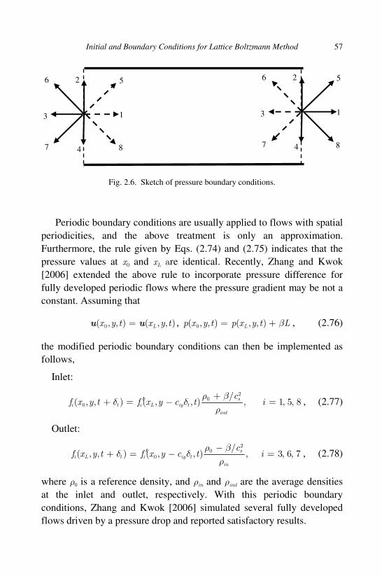
Initial and Boundary Conditions for Lattice Boltzmann Method 57
Periodic boundary conditions are usually applied to flows with spatial
periodicities, and the above treatment is only an approximation.
Furthermore, the rule given by Eqs. (2.74) and (2.75) indicates that the
pressure values at x0 and xL are identical. Recently, Zhang and Kwok
[2006] extended the above rule to incorporate pressure difference for
fully developed periodic flows where the pressure gradient may be not a
constant. Assuming that
0( , , ) ( , , )Lx y t x y t=u u , 0( , , ) ( , , )Lp x y t p x y t Lβ= + , (2.76)
the modified periodic boundary conditions can then be implemented as
follows,
Inlet:
20
0
/( , , ) ( , , ) , 1, 5, 8si t i L iy t
out
cf x y t f x y c t i
ρ βδ δ
ρ
+′+ = − = , (2.77)
Outlet:
2
00
/( , , ) ( , , ) , 3, 6, 7si L t i iy t
in
cf x y t f x y c t i
ρ βδ δ
ρ
−′+ = − = , (2.78)
where ρ0 is a reference density, and ρin and ρout are the average densities
at the inlet and outlet, respectively. With this periodic boundary
conditions, Zhang and Kwok [2006] simulated several fully developed
flows driven by a pressure drop and reported satisfactory results.
Fig. 2.6. Sketch of pressure boundary conditions.
8
1
5 6
7 4
2
3
8
1
5 6
7 4
2
3

58 Lattice Boltzmann Method and Its Applications in Engineering
2.4.2 Hydrodynamic schemes
With the idea of bounce-back of non-equilibrium distribution functions,
Zou and He [1997] developed a hydrodynamic scheme for pressure
boundary conditions. As shown in Fig. 2.6, for the D2Q9 model the
unknown distribution functions f 1, f 5, and f 8 at the inlet are determined
from the following conditions,
1 5 8 0 2 3 4 6 7( )inf f f f f f f f fρ+ + = − + + + + + , (2.79)
1 5 8 3 6 7/in inf f f u c f f fρ+ + − = + + , (2.80)
5 8 2 4 6 7f f f f f f− = − + − + , (2.81)
( ) ( )1 1 3 3
eq eqf f f f− = − , (2.82)
where the velocity at the inlet is ( , 0)in inu=u and it is unknown, while
the density at the inlet, inρ , can be obtained from the specified pressure.
By solving this set of equations, one can get the unknown distributions at
the inlet, and those at the outlet can be determined similarly.
2.4.3 Extrapolation schemes
Based on the extrapolation technique, Chen et al. [1996] devised a
simple extrapolation scheme for pressure boundary conditions similar to
that for velocity boundary conditions. Again consider the inlet shown in
Fig. 2.6, a ghost layer is appended to the layer at the inlet, and the
distribution functions at the ghost layer are approximated by
( 1) 2 (0) (1)i i if f f− = − , (2.83)
where −1, 0, and 1 are the labels for the ghost layer, the inlet, and the
first fluid layer, respectively. Then the collision process can be carried
out on all nodes including the ghost ones, but it should be noted that the
specified pressure/density is used in calculating the EDFs at the inlet.
Maier et al. [1996] also presented a similar method.
The non-equilibrium technique can also be used to treat pressure
boundary conditions. In this case the unknown distribution functions at
the inlet are again decomposed into two parts, where the equilibrium part

Initial and Boundary Conditions for Lattice Boltzmann Method 59
is approximated by
( ) ( )ˆ ( , ) ( , ), 1, 5, 8eq eqi b i in inf t f iρ= =x u , (2.84)
where 0 0( ) ( )in f i tδ= +=u x u x x c is the velocity at the nearest
neighboring fluid node along the particle velocity. The non-equilibrium
part is approximated by that at the same fluid node, too. The final
expressions of the unknown distribution functions then read,
( ) ( )( , ) [ , ( , )] [ ( , ) ( , )], 1, 5, 8eq eqi b i in f i f i ff t f t f t f t iρ= + − =x u x x x . (2.85)
Similar to the analysis for the non-equilibrium extrapolation schemes for
velocity boundary conditions, it can be shown that this scheme is also of
second-order accuracy. Also, because only first order extrapolations are
involved, this scheme has good numerical stability as well [Guo et al.,
2002a].
2.5 Summary
In this chapter we have discussed the initial and boundary conditions in
LBE, which are fundamental topics in this field. For initial conditions,
two main approaches are presented, i.e. the earlier non-equilibrium
correction method and the recent iterative method. Some schemes for
velocity and pressure boundary conditions, which are widely used in the
applications of LBE, are also described.
It is noted that the simple equilibrium schemes are not discussed in
the above sections, since it is quite straightforward to implement such
boundary conditions. For example, when the pressure is given, with an
extrapolated velocity, the EDFs can be approximately used in the
required unknown directions. Some theoretical studies of boundary
conditions for LBE, were not detailed in this chapter, either. For instance,
He et al. [1997] found the analytical solutions of the LBE under different
boundary conditions, based on which the accuracies of the schemes were
analyzed. Junk and Yang [2005a] made an asymptotic analysis of the
bounce-back, BFL, FH, and MLS schemes. Kao and Yan [2008]
compared the FH, BFL, and YMS schemes, and developed a scheme

60 Lattice Boltzmann Method and Its Applications in Engineering
without interpolation. On the other hand, Suh et al. [2008] performed
theoretical and numerical comparisons of the YMS, BFL, and non-
equilibrium extrapolation schemes for curved walls. Some new boundary
schemes are also developed from different pictures [Junk and Yang,
2005b; Chun and Ladd, 2007]. In summary, developing accurate,
effective, and simple schemes for initial and boundary conditions is still
a very active branch in LBE.

61
Chapter 3
Improved Lattice Boltzmann Models
In Chapter 1, we have described the general LBE models for isothermal
flows. These models (particularly the DnQb LBGK models), together
with the initial and boundary conditions introduced in Chapter 2, have
been successfully applied to many simple and complicated flow
problems. However, there is still much space to improve the performance
of these models, and in this chapter we will give a few examples.
3.1 Incompressible Models
As shown in Chapter 1, the hydrodynamic equations derived from the
LBE equation are actually the compressible Navier-Stokes equations.
Meanwhile, the intrinsic low Mach number requirement of LBE indicates
that it is limited to nearly incompressible flows. Therefore, the LBE
can be viewed as a special artificial compressibility method for
incompressible flows [He et al., 2002; Ohwada et al., 2011]. As such, a
numerical error related to the artificial compressibility will arise in
addition to those from the spatial and temporal discretization. The
compressible effect may lead to significant errors in some cases. For
instance, in a comparative study of a two-dimensional turbulent flow
[Zou et al., 1995], Martinez et al. found that the LBE results deviated
greatly from the spectral data at the late stage, and they attributed this
deviation to the compressible effects of the LBE.
In order to reduce the compressible effects in LBE, some
modifications to the standard models have been developed from different
viewpoints, and we will call such models as incompressible LBE models
although they may still contain some compressibility errors. In 1995, Zou
and his coworkers made the first attempt to construct an incompressible

62 Lattice Boltzmann Method and Its Applications in Engineering
D2Q9 model for steady flows. In this model, the evolution equation is
the same as the standard LBGK model, but the discrete EDF is re-
defined as
2 2
( )
2 4 2
( )
2 2
ieq ii i
s s s
fc c c
ω ρ⋅
= + + −
⋅ u uuc c. (3.1)
It can be seen that this EDF is very similar to that of the standard D2Q9
model except that the density is decoupled from the momentum. The
fluid density and velocity in Zou’s model are calculated as
,i i i
i i
f fρ = =∑ ∑u c . (3.2)
The hydrodynamic equations derived from Zou’s model via the
Chapman-Enskog expansion read,
0tρ∂ + ∇ ⋅ =u , (3.3)
( )( ) Tpt
ρν∂ + ∇ ⋅ = −∇ + ∇ ⋅ ∇ + ∇ ∂u
uu u u , (3.4)
where the pressure p and the kinematic viscosity are both the same as the
standard D2Q9 model. It is clear that Eqs. (3.3) and (3.4) reduce to the
standard incompressible Navier-Stokes equations at steady state, namely,
the compressible effects are removed totally.
It is noted that in Zou’s incompressible model, the pressure is still
related to the fluid density. Sometime later, Lin et al. [1996] proposed a
similar incompressible model which used a density-independent pressure.
Numerical results show that Zou’s model works well for steady flows.
But for unsteady flows, this model still contains compressibility error.
Chen and Ohashi [1997] extended Zou’s model for general flows by
introducing a correction to the velocity defined by Eq. (3.2). That is, the
flow velocity is
φτ∇= +w u , (3.5)
where φ is a scalar to be determined. In order to enforce w to be
divergent free, φ should satisfy the following Poisson equation,
2 1φ
τ∇ = − ∇ ⋅ u . (3.6)

Improved Lattice Boltzmann Models 63
After solving the above equation, one can obtain the fluid velocity w
according to Eq. (3.5).
It is noted that in the Chen-Ohashi model, the fluid velocity appearing
in the discrete EDF is w instead of u. The Chapman-Enskog expansion of
this model leads to the exact incompressible Navier-Stokes equations
for w, and the pressure is given by 2sp c ρ φ= − . The basic idea of the
velocity correction method employed in the Chen-Ohashi model is
similar to the pressure-correction method for incompressible Navier-
Stokes equations in traditional CFD method. Because the Laplacian
operator in the Poisson equation (3.6) is non-local, the computational
costs of the Chen-Ohashi model will be greater than Zou’s model.
Almost at the same time when Chen-Ohashi model was proposed, He
and Luo [1997] developed another general incompressible LBGK model.
The basic idea is to remove terms of high-order Mach number due to
density variations in the EDF. In this model, the independent variables
are the pressure and velocity rather than the density and momentum.
As known, the density variation of the density, 0/δρ ρ , in nearly
incompressible flows is of order M
2, where 0ρ is a averaged density.
Therefore, the standard EDF of the DnQb models can be approximated as
( ) 30 0
0
1 ( ) ( ) ( )eqi i i i if s s O M
δρω ρ ρ ω ρ ρ
ρ
= + + = + + u u , (3.7)
where si is the collective of the velocity terms in the EDF,
2 2
2 4 2
( )( )
2 2
iii i
s s s
sc c c
ω ⋅⋅ = + −
c uc u uu . (3.8)
Therefore, after neglecting the O(M
3) terms, and let ( ) ( )2eq eqi s ip c f= , one
can obtain a pressure EDF,
2 2
( )0 2 4 2
( )
2 2
ieq ii i
s s s
p pc c
pc
ω = + + −
⋅
⋅ uu ucc, (3.9)
where 2sp c ρ= and
20 0sp c ρ= , and the evolution equation of the He-Luo
model is,
( )( , ) ( , ) ( , ) ( ,1
)eqi i t t i i it p t p pp t tδ δ
τ + + − = − − x c x x x , (3.10)

64 Lattice Boltzmann Method and Its Applications in Engineering
while the pressure and velocity are defined by
0,i i i
i i
p pp p= =∑ ∑u c . (3.11)
The hydrodynamic equations derived from the He-Luo model are
2
10t
s
Pc
∂ + ∇ ⋅ =u , (3.12)
2Pt
ν∂
+ ⋅ ∇ = −∇ + ∇∂u
u u u , (3.13)
where 0/P p ρ= . It is clear that Eqs. (3.12) and (3.13) are just the artificial
compressible version of the incompressible Navier-Stokes equations. The
solution of the above equations can be a good approximation to that of
the incompressible Navier-Stokes equations provided that the first term
in Eq. (3.12) can be neglected. In order to see how this can be achieved,
we rewrite Eq. (3.12) in dimensionless form,
0
0s
L P
c t t
′∂ ′ ′+ ∇ ⋅ =′∂
u , (3.14)
where the nondimensional variables with a prime are defined by,
sc
′ =u
u , 2s
PP
c′ = ,
0
tt
t′ = ,
L′ =x
x , (3.15)
with t0 and L being the characteristic time and length, respectively.
Therefore, in order to neglect the transient term in Eq. (3.14), it is
required that 0 / st L c .
The He-Luo model has the same structure as the standard LBGK
method and shares all of its advantages. Particularly, in this model the
pressure behaves as an independent variable and can even take negative
values. Actually, in some works the pressure in the EDF (3.9) is defined
from the density variation directly, i.e. 2sp c δρ= . In this regard, p acts as
a dynamic pressure rather than a thermodynamic one.
Guo et al. [2000] developed another pressure-based incompressible
LBGK model later. Unlike the previous incompressible models which
Improved Lattice Boltzmann Models 65
are based on the original density-based models, Guo’s model is designed
with intent to solve the incompressible Navier-Stokes equations directly.
The EDF in Guo’s D2Q9 model reads,
02
( )
2
2
4 ( ), 0
( ), 1, 2, 3, 4
( ), 5, 6, 7, 8
eqi i
i
Ps i
c
Ps i
c
ic
g
Ps
σ
λ
γ
− + == + = + =
u
u
u
(3.16)
where si is defined by Eq. (3.8), and the parameters σ, λ, and γ satisfy
the following relation
, 2 4 1λ γ σ λ γ+ = + = . (3.17)
With this EDF, the evolution equation of Guo’s model is expressed as
( )( , ) ( , ) ( , ) ( ,1
)eqi i t t i i it g t g gg t tδ δ
τ + + − = − − x c x x x , (3.18)
and the pressure and velocity are defined by
2
0, ( )4
i i i
i i
gc
P sgσ
= = +
∑ ∑cu u . (3.19)
The Chapman-Enskog expansion of this model leads to the exact
incompressible Navier-Stokes equations,
0∇ ⋅ =u , (3.20)
2Pt
ν∂
+ ⋅ ∇ = −∇ + ∇∂u
u u u , (3.21)
where the shear viscosity is the same as the standard D2Q9 model.
The above incompressible LBGK models can be easily extended to
MRT models. For example, the MRT version of the He-Luo model has
been proposed in [d'Humières et al., 2002], while the MRT version of
Guo’s model was reported in [Du et al., 2006].

66 Lattice Boltzmann Method and Its Applications in Engineering
3.2 Forcing Schemes with Reduced Discrete Lattice Effects
Fluid flows are usually exposed to external or internal forces, such as
gravity or intermolecular interactions. In the continuous Boltzmann
equation, the contribution of a body force ρ=F a , where a is the force
acceleration, to the change of the distribution function f is described by a
forcing term ( , , )f t⋅ ∇a xξ ξ . In LBE, however, this forcing term cannot
be employed straightforwardly because the particle velocity is discretized.
Therefore, it is a fundamental topic to include such forces into the LBE,
and a variety of discrete forcing schemes have been developed from
different physical pictures. For convenience, we will express the EDF as
a function of the fluid density and velocity,
2 2
( )
2 4 2
( )( , ) ( , ) 1
2 2
ieq ii i i
s s s
f t Ec c c
ρ ω ρ ⋅⋅ = ≡ + + −
c uc u ux u . (3.22)
3.2.1 Scheme with modified equilibrium distribution function
If the force is induced by a potential and the density variation is small, i.e.
F = −ρ∇φ ≈ −∇(ρφ ), it can be included into the LBE by modifying the
EDF [Buick and Greated, 2000],
2
( )0 02 20
( )1 (1 )
2
eq
s s
p uf
c c
φρ ω ω
ρ
= − − −
,
2 2
( )
2 2 4 2
( ) ( ), 0
2 2
ieq ii i
s s s s
p uf i
c c c c
φω ρ
ρ
= + + −
⋅≠
⋅
c uc u (3.23)
where 2( )sp c φ ρ= + , and u is defined by
i i
i
fρ = ∑u c . (3.24)
It is easy to verify that the zeroth, first, and third order moments of ( )eqif
are the same as those of the standard DnQb models (c.f. Eq. (1.52)), but
the second-order moment involves the potential,
( ) ( )eqi i i
i
c c f p u uα β αβ α βφ δ ρ= +∑ . (3.25)

Improved Lattice Boltzmann Models 67
With this change, we can show that the momentum flux at the order of
ε in the Chapman-Enskog expansion is (neglecting the terms of O(M 2)),
( )
( )0
(1) 20 0 0
0 0
( )
( ) ( )
t s tc u u
u u
α β β α ααβ
β α β β α
π τδ ρ ρφ
ρφ ρφ
= − ∂ + ∂ + ∂ ∂− ∂ ∂ + ∂ . (3.26)
Therefore, the momentum equation will be
( )2( )
( ) ( ) Tsc R
t
ρρ ρ ρν
∂ + ∇ ⋅ = −∇ + ∇ ⋅ ∇ + ∇ + + ∂u
uu u u F , (3.27)
where the residual term R is given by
( )t t uF F u FR β α β βα ατδ = − +∂ + ∂ . (3.28)
Clearly, R does not vanish in general, and so the above method will bring
some additional errors due to the force field.
The force can also be included in LBE by modifying the fluid
velocity appearing in the EDF [Shan and Chen, 1993], namely, the
equilibrium velocity is now given by,
( )eqtτδ= +u u a . (3.29)
In the original method developed by Shan and Chen (referred to SC)
[1993], the fluid velocity u is still defined by Eq. (3.24). In a later work,
it was argued that the fluid velocity (denoted by v for clarity) should be
defined as the average of pre- and post-collision velocities (referred to
SD scheme) [Shan and Doolen, 1995],
1
( )2 2
ti i i
i
f fδ
ρ ρ′= + = +∑v c u F . (3.30)
3.2.2 Schemes with a forcing term
The most straightforward way to account for the body force is to add a
forcing term to the LBE, like that in the Boltzmann equation,
( )( , ) ( , ) ( ) ( ,1
, )eqi i t t i i i t it f t t f tf f Fδ δ δ
τ + + − = − − + x c x x x , (3.31)

68 Lattice Boltzmann Method and Its Applications in Engineering
where the forcing term Fi depends on the body force F. A variety of
expressions for Fi have been proposed with different interpretations of
the fluid velocity.
Scheme based on LGA
The early widely used forcing scheme originates from the LGA method
[Frisch et al., 1987; Luo, 1997], which can be written as,
2
ii i
s
Fc
ω⋅
=c F
. (3.32)
This forcing scheme is constructed to enforce mass and momentum
conservations [Frisch et al., 1987; Luo, 1997],
0i
i
F =∑ , i i
i
F =∑c F . (3.33)
In this forcing scheme, the EDF and the fluid velocity are both the same
as the standard DnQb models, i.e. ( ) ( , )eqi if E ρ= u and the fluid velocity
is still defined by Eq. (3.24). It was also suggested by some researchers
that the fluid velocity takes v instead of u [Ginzbourg and Adler, 1994],
and we will call this scheme as modified LGA scheme and denoted by
mLGA.
Buick-Greated scheme
In this scheme the forcing term is defined by [Buick and Greated, 2000],
2
11
2i i
s
iFcτ
ω ⋅ −
=c F
, (3.34)
while the fluid velocity is defined again as the average of the pre- and
post-collision velocities,
2
ti i
i
f= +∑ Fv c
δρ , (3.35)
which is also used in the EDF, i.e. ( ) ( , )eqi if E ρ= v .
He-Shan-Doolen scheme
This model (denoted by HSD) was developed based on the continuous
Boltzmann equation [He et al., 1998]. The forcing term in the continuous
Improved Lattice Boltzmann Models 69
velocity space is first approximated as,
( ) ( )
2
( )( , , ) ( , , ) ( , , )eq eq
s
f t f t f tc
− ⋅⋅ ∇ ≈ ⋅ ∇ = −
v aa x a x xξ ξ
ξξ ξ ξ , (3.36)
where ( )( ) ( )( , , ) ; ( , ), ( , )eq eqf t f t tρ=x x v xξ ξ is the equilibrium distribution
function given by
2
( )
/2
( )exp
(2 ) 2eq
Df
RT RT
ρ
π
− = −
vξ, (3.37)
and here D is the spatial dimension. Following the standard discretization
procedure as given in Chapter 1, one can obtain a discrete velocity model
with a forcing term,
( )1 eqii i i i i
c
ff f f F
t τ
∂ + ⋅ ∇ = − − + ∂c , (3.38)
where the forcing term is given by
( )
2
( )i eqi i
s
Fc
f− ⋅
=c v a
, (3.39)
with 2sc RT= being the sound speed, and
( ) ( , )eqi if E ρ= v . The density
and velocity of the fluid are given by
i
i
fρ = ∑ , i i
i
fρ = ∑v c . (3.40)
Integrating Eq. (3.38) along the characteristic line leads to
0
( , ) ( , ) ( , )t
i i t t i i if t f t t t t dtδ
δ δ ′ ′ ′+ + − = Λ + +∫x c x x c , (3.41)
where
( )1 eqi i i i
c
f f Fτ
Λ = − − + . (3.42)
Evaluating the integral on the right hand side of Eq. (3.41) using the
trapezoidal rule one can obtain that
( , ) ( , ) ( , ) ( , )2
ti i t t i i i t t if t f t t t
δδ δ δ δ + + − = Λ + + + Λ x c x x c x . (3.43)

70 Lattice Boltzmann Method and Its Applications in Engineering
The above scheme is implicit. However, the implicitness can be eliminated
by introducing the following distribution function,
( , ) ( , )2
ti i if f t t
δ= − Λx x . (3.44)
Equation (3.43) can then be rewritten as Eq. (3.31) with τ = τc/δt + 1/2, and
( )
2
( )1 ( , )
2
ieqi i
s
f Ec
ρ − ⋅ = −
c v av . (3.45)
From Eq. (3.44) we can see that the density and velocity of the fluid can
be computed from the new distribution function directly,
i if fι ι
ρ = =∑ ∑ , 2
ti i i if f
ι ι
δρ = = +∑ ∑v c c F . (3.46)
It is also noted that the term associated with the force in the EDF given
by Eq. (3.45) can be regrouped into the forcing term so that the He-Shan-
Doolen forcing scheme becomes
( ) ( )
2
( )1( , ), 1
2
ieq eqi i i i
s
f E F fc
ρτ
− ⋅= = − c v a
v . (3.47)
Moment-expansion scheme
Luo noted that although the forcing term ( , , )f t⋅ ∇a xξ ξ in the Boltzmann
equation cannot be discretized in the discrete velocity space, the first
three moments of this term can be written out explicitly [Luo, 1998],
0,
,
( ) .
f d
f d
f d
ρ
ρ
⋅ ∇ =
⋅ ∇ = −
⋅ ∇ = − +
∫
∫
∫
a
a a
a au ua
ξ
ξ
ξ
ξ
ξ ξ
ξξ ξ
(3.48)
Therefore, the forcing term can be expanded as a series of ξξξξ,
(0) (1) (2)( ) :f cρω ⋅ ∇ = + ⋅ + + a c c ξ ξ ξ ξξ , (3.49)
where
2
2 /2 2
1( ) exp
(2 ) 2Ds sc c
ωπ
− = ξ
ξ , (3.50)
Improved Lattice Boltzmann Models 71
and the expansion coefficients are
(0)
2s
cc
⋅= −a u
, (1)
2sc
= −a
c , ( )(2)
4
1
2 sc= − +c au ua . (3.51)
Substituting these results into Eq. (3.49) we can express the forcing term
explicitly, which further leads to the following discrete forcing scheme,
2 4
( )i iii i
s s
Fc c
ω ρ ⋅− = + ⋅
c u cc ua . (3.52)
It is noted that in the moment-expansion scheme, the fluid velocity v is
the same as u.
The moment-expansion scheme was also obtained independently by
Martys et al. [1998] based on Hermite expression of the distribution
function, and Shan et al. [2006] made a further extension by including
higher-order moments. It is also noted that if only the zeroth moment is
considered in the expansion, the moment-expansion scheme reduces to
the scheme based on the LGA method.
Modified moment-expansion schemes
Ladd and Verberg [2001] proposed another two moment-expansion
schemes (denoted by LV-I and LV-II, respectively), which can be
expressed as,
( )2
2 4
:
2
i i sii i
s s
cF
c cω
−⋅ = +
C c c IB c. (3.53)
The coefficients and the EDF are
( )
( )
1, 1 ( ), ,
2
( , );
LV-2: , ,
LV-1:
,
(
,2
, ).
i i
ieq
i i
ti i
ieq
i i
f
f E
f
f E
ρ ρτ
ρ
δρ
ρ
= = − + = = =
= = + = = +
=
∑
∑
B F uF Fu v u
u
B F uF Fu u a
C c
c v u
u
C
(3.54)
Later, Guo et al. [2002c] proposed another moment-expansion scheme
(denoted by GZS) which has the same formulation as Eq. (3.53) and the

72 Lattice Boltzmann Method and Its Applications in Engineering
coefficients are given by
1 1
1 , 1 ( ),2 2τ τ
= − = − + B F C vF Fv
( ), ( , ).2
eqti i i i
i
f f Eδ
ρ ρ= + =∑cv F v (3.55)
3.2.3 Analysis of the forcing schemes
We now make an analysis of the LBE with a forcing scheme through
the Chapman-Enskog expansion method. The derived hydrodynamic
equations will contain some additional terms due to the forcing term in
comparison with the standard Navier-Stokes equations, through which
we can evaluate the accuracy of the forcing schemes.
First, we express the forcing schemes (except for the HSD scheme)
given in previous sections in a general formulation,
( ) ( )
( )
* * 2
2 4
* 2
2 4
:
2
:,
i i sii i
s s
i i sii
s s
C cBF
c c
C cB
c c
+ −⋅ = + −⋅ = +
u F Fu c c IF c
u F c c IF c
ω
ω
(3.56)
together with the following EDF, equilibrium velocity u*, and fluid
velocity v,
( ) * * ,( , ),eqi i i i t i i t
i i
f E f m f lρ ρ δ ρ δ= = + = +∑ ∑u F vc cu F , (3.57)
where B, C, m, and l are scalar parameters. It can be easily shown that
* *0, , ( )i i i i i i
i i i
F F B F C= = = +∑ ∑ ∑c c c u FuF F . (3.58)
In Tab. 3.1 the parameters of different forcing schemes are listed. It is
noted the HSD scheme can also be expressed as Eq. (3.56) together with
some terms of O(u2), and the zeroth- and first-order moments are also the
same as those given in Eq. (3.58), but the second-order moment is
*
*
2
* * *( )1
12
i i i
i s
Fc
⋅ = − − +∑ u
c c u F u uF
Fuτ
. (3.59)
Improved Lattice Boltzmann Models 73
After neglecting the term of order O(u3), it can be seen that the
parameters of the HSD and GZS schemes are just the same, although
their expressions are different.
With the general formulation, the LBE with a forcing term can be
expressed as
*1( , ) ( , ) ( , ) ( , ) ( , )i i t t i i i t if t f t f t E F tδ δ ρ δ
τ + + − = − − + x c x x u x . (3.60)
The hydrodynamics equations can be derived from Eq. (3.60) following
the standard Chapman-Enskog expansion method. With the expansions
given by Eq. (1.53), the equations of the Taylor series expansion of
Eq. (3.60) can be expressed at each time scale as,
0 :ε (0) *( , )i if E ρ= u , (3.61)
1 :ε (0) (1) (0)0
1i i i i
c
D f f Fτ
+= − , (3.62)
2 :ε 1
(0) (1) (0) (2)20 0
1
2
tt i i i i i i
c
f D f D f fδ
τ∂ + + = − , (3.63)
Table 3.1. Parameters of the forcing schemes.
Scheme m l B C
LGA 0 0 1 0 mLGA 0 1/2 1 0 SC τ 0 0 0
SD τ 1/2 0 0
BG 1/2 1/2 (2τ−1) /2τ 0
Luo 0 0 1 1
LV-I 0 0 1 (2τ−1) /2τ
LV-II 0 1/2 1 1
GZS 1/2 1/2 (2τ−1) /2τ (2τ−1) /2τ
HSD* 1/2 1/2 (2τ−1) /2τ (2τ−1) /2τ
*The second-order moment of the HSD scheme is 2* * * * *( )/ scC − ⋅+u F Fu uF u u .
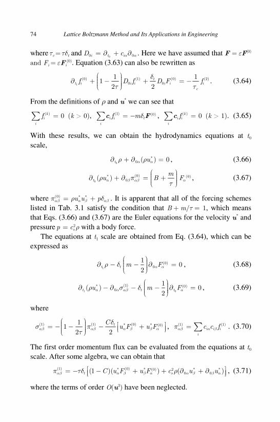
74 Lattice Boltzmann Method and Its Applications in Engineering
where τc = τδt and 00 0i t iD c α α= ∂ + ∂ . Here we have assumed that F = εF(0)
and Fi = εFi(0). Equation (3.63) can also be rewritten as
1
(0) (1) (0) (2)0 0
1 11
2 2
tt i i i i i i
c
f D f D F fδ
τ τ
∂ + − + = − . (3.64)
From the definitions of ρ and u* we can see that
( ) 0ki
i
f =∑ (k > 0), (1) (0)i i t
i
f mδ= −∑c F , ( ) 0ki i
i
f =∑c (k > 1). (3.65)
With these results, we can obtain the hydrodynamics equations at t0
scale,
0
*0 ( ) 0t uα αρ ρ∂ + ∂ = , (3.66)
0
(0)* (0)( )t
mu B Fαα β αβρ π
τ0
∂ + ∂ = + , (3.67)
where (0) * *u u pα β αβαβπ ρ δ= + . It is apparent that all of the forcing schemes
listed in Tab. 3.1 satisfy the condition that B + m/τ = 1, which means
that Eqs. (3.66) and (3.67) are the Euler equations for the velocity u* and
pressure 2sp c ρ= with a body force.
The equations at t1 scale are obtained from Eq. (3.64), which can be
expressed as
1
(0)0
10
2t t m Fααρ δ
∂ − − ∂ = , (3.68)
1 0
((10
)* 0) 1( ) 0
2t t t Fu m
∂ − ∂ − − ∂ = αα α αβρ σ δ , (3.69)
where
(1) (1) (0)* * (0)11
2 2
tCu F u F
= − − − + α β ααβ αβ β
δσ π
τ, (1) (1)
i i i
i
c c fα βαβπ = ∑ . (3.70)
The first order momentum flux can be evaluated from the equations at t0
scale. After some algebra, we can obtain that
(1) (0)* * (0) 2 * *0 0(1 )( ) ( )t sC u F u F c u u = − − + + ∂ + ∂ α β α α β β ααβ βπ τδ ρ , (3.71)
where the terms of order O(u3) have been neglected.

Improved Lattice Boltzmann Models 75
Combining the equations at t0 and t1 time scales we can obtain the
following hydrodynamic equations
* 1( )
2t m
t
ρρ δ
∂ + ∇ ⋅ = − ∇ ⋅ ∂u F , (3.72)
** * *
* *
( ) 1( ) (2 )
21
( ) ,2
t
t
p mt t
C
∂ ∂+ ∇ ⋅ = −∇ + ∇ ⋅ + + − ∂ ∂ + ∇ ⋅ − − +
u Fu u S F
u F Fu
ρρ ρ δ
δ τ τ
υ
(3.73)
where * * *( ) / 2S u uαβ α β β α= ∂ + ∂ , and we have assumed that ε∂F/∂t0 ≈
∂F/∂t or ε2∂F/∂t1 = 0. The above equations can also be written in terms
of the fluid velocity v
by noticing that * ( ) tl m δ= + −v u a ,
( ) Rt
ρ
ρρ
∂+ ∇ ⋅ =
∂v , (3.74)
( )
( ) (2 ) vp Rt
ρρ ρν
∂+ ∇ ⋅ = −∇ + ∇ ⋅ + +
∂v
vv S F , (3.75)
where Rρ and Rv are the residual terms that reflect the derivations of the
derived hydrodynamic equations from the desired mass and momentum
conservation equations. These terms can be written out explicitly as,
1
2tR lρ δ = − ∇ ⋅
F , (3.76)
1( ) (2 )
21
( ) ( ) ,2
tv
t
lt
C
∂ ′ ′ ′ ′ ′= − − ∇ ⋅ + + + ∇ ⋅ ∂ ′ ′+ ∇ ⋅ − − + + +
Fvu u v u u S
vF Fv u F Fu
R δ ρ ρν
δ τ τ
(3.77)
where u' = (m − l )aδt and ( ) / 2S u uαβ α β β α
′ ′ ′= ∂ + ∂ . It is clear that
different forcing schemes will give different residuals. In Tab. 3.2 Rρ and
Rv are listed for some forcing schemes.
It is clear that most of the forcing schemes give nonvanishing
residuals in the mass and momentum conservation equations.
Specifically, only those using v = ∑i ci fi + Fδt /2 (i.e. l = 1/2) as the fluid
velocity satisfy the mass conservation equation in general, and the
spurious velocity u' due to the body force vanishes only when the
equilibrium velocity u* is taken as the fluid velocity v (i.e m = l );

76 Lattice Boltzmann Method and Its Applications in Engineering
Furthermore, it is found that the force contribution to the momentum flux
does not appear only when C = 1 − 1/2τ. It is apparent that only the
GZS and HSD schemes satisfy these constraints and yield the correct
hydrodynamics equations. It is also noted that when the acceleration a is
a constant and the density changes slowly in both time and space, the
continuity equation holds for all of the forcing schemes, and the terms of
temporal/spatial derivatives of the force in the momentum equation can
be neglected, which means that the SD, LV-I, and LV-II schemes also
give the desired hydrodynamic equations. On the other hand, the residual
term Rv in the momentum equation of the other five schemes does not
disappear even in such case due to the coupling terms vF and Fv.
3.2.4 Forcing scheme for MRT-LBE
The forcing schemes for the LBGK models can be easily extended to
MRT-LBE models. For example, Guo and Zheng [2007] have extended
Table 3.2. Residual terms of the hydrodynamics equations for some forcing schemes.
Scheme Rρ vR
LGA 2
tδ− ∇ ⋅ F ( ) ( )1
2 2
t
t t− ∂ + − ∇ ⋅ +F vF Fvδ
δ τ
mLGA 0 ( ) ( ) ( )12 4
Tt t
µδ τ δ τ ρ − ∇ ⋅ ∇ + ∇ − + + − a a vF Fv aa
SC 2
tδ− ∇ ⋅F ( ) ( )
2
2 ( 1)
t
t
T
t t
t
∇ + ∇ − + − ∂ + ∇ ⋅ + −
a a vF FvF
aa
δ
δ τµδ
δ τ τ ρ
SD 0 ( ) ( ) ( )1 1
2 2
Tt tδ τ µ δ τ ρ − ∇ ⋅ ∇ + ∇ + − a a aa
BG 0 ( ) ( )1
2tδ τ − ∇ ⋅ +vF Fv
Luo 2
tδ− ∇ ⋅F ( )2 2
t t
tδ δ− ∂ − ∇ ⋅ +F vF Fv
LV-I 2
tδ− ∇ ⋅F 2
t
tδ− ∂ F
LV-II 0 ( )2 2
t tT − ∇ ⋅ ∇ + ∇ + a a aaδ δ
µ ρ
GZS 0 0
HSD 0 0

Improved Lattice Boltzmann Models 77
the GZS scheme to MRT-LBE recently, and the evolution equation with
a forcing term is written as
1 ( ) 1 ˆ( , ) ( , ) [ ]eqi t t tt tδ δ δ− −+ + − = − − +f x c f x M SM f f M F , (3.78)
for i = 0, 1, …, b − 1, where M is the transform matrix, S = diag(s0, s1, …,
sb-1) is the relaxation matrix, and F is the moments of the forcing term in
the moment space which can be expressed as
1ˆ2
= − F I S MF , (3.79)
where ( )0 1 1, , ,T
bF F F −=F is related to the body force F,
2
2 4
: ( )i i si i
s s
i cF
c cω
− = +
⋅
vF c c Ic F, (3.80)
and here the fluid velocity v is defined by Eq. (3.55). Obviously, when
si = 1/τ the forcing scheme reduces to that for the LBGK model. The
forcing moments can be computed explicitly. For example, for the D2Q9
MRT model the nine moments are
0 0F = , 1 6 12
esF = − ⋅
v F , 2 6 12
sF ε
= − − ⋅ v F , 3 xF F= ,
4 12
q
x
sF F
= − − , 5 yF F= , 6 1
2
q
y
sF F
= − − ,
7 2 1 ( )2
x x y y
sF v F v Fν
= − − , 8 1 ( )
2x y y x
sF v F v Fν
= − + .
With the forcing moments, the collision process of a MRT-LBE can
be implemented in moment space as
( ) ˆ( , ) ( , ) ( , ) eqk k k k t ikm t m t s m t m Fδ ′ = − − + x x x . (3.81)
Then the post-collision moments are transformed back to the velocity
space where the standard streaming process is carried out.
The Chapman-Enskog expansion of Eq. (3.78) together with the
forcing term given by Eq. (3.79) leads to the correct hydrodynamics
equations, where the shear and bulk viscosities are the same as those

78 Lattice Boltzmann Method and Its Applications in Engineering
given in Chapter 1. It is noted that the above forcing scheme is closely
related to that for the LBGK model. But due to the freedom of MRT
models, the forcing scheme can also be constructed directly in moment
space.
3.3 LBE with Nonuniform Grids
The standard LBE models utilize certain regular lattices associated with
the discrete velocities as the computational meshes. The flexibility of
such meshes is rather limited, particularly for flows with irregular
geometries. The choice of the computational meshes as the underlying
lattice is not essential, however. Such choice is mainly due to historic
reasons that LBE is a descendant of the LGA method which utilizes a
regular lattice. Once the fact that LBE is a special finite-difference
scheme of the continuous Boltzmann equation is recognized, we can
decouple the computation mesh from the underlying lattice.
A number of LBE methods using irregular meshes have been
developed in the past years. The method can be classified into six types:
(1) Grid-refinement and multi-block methods, (2) interpolation methods,
(3) finite-difference based methods (FD-LBE), (4) finite-volume based
methods (FV-LBE), (5) finite-element based methods (FE-LBE), (6)
Taylor series expansion and least square-based methods (TLLBE). In this
section we will present some examples of these non-standard LBE
methods.
3.3.1 Grid-refinement and multi-block methods
Grid-refinement technique is widely used in CFD methods to treat the
regions where flow variables change rapidly. The main advantage of the
grid refinement method is that the boundary information can be spread to
the flow domain quickly on the coarser grid and the overall flow pattern
can be captured with low computational costs. The detailed information
in the regions where large gradients exist can be captured more
accurately on the refined grid. This technique was introduced into LBE
first by Filippova and Hänel (referred to as FH) [1998]. In their method a

Improved Lattice Boltzmann Models 79
coarse mesh is first used to cover the flow domain, and then one or
several patches with refined resolutions will be inserted into some
regions on where the flow may change significantly. Different patches
can be used in different regions, and nest refinements can be employed if
necessary. As an example, in what follows we will consider a mesh
composed of a coarse lattice with spacing cxδ and a fine one with
spacing fxδ , and assume that /c f
x xn δ δ= is an integer.
The evolutions on the coarse and fine grids can be written as
( )1( , ) ( , ) ( , ) ( , )eqk k k k k k k k k
i i t t i i ikf t f t f t f tδ δ
τ + + − = − − x c x x x , (3.82)
where the variables with a superscript k = c or f represent quantities on
the coarse or fine grid. Note that the EDF is identical on both coarse and
fine grid since it depends only on the grid-independent variables (sound
speed, fluid density, and velocity). Furthermore, since the sound speed
and viscosity of the fluid should be independent of the meshes, the
following relations must hold,
1 1 1
,2 2
f c f ct t n
nδ τδ τ
= = + − . (3.83)
On the other hand, from the Chapman-Enskog analysis we can see that
the nonequilibrium parts of the distribution functions on the nodes shared
by both grids satisfy the following condition,
,( ) ,( )
(0) ( )( , )c neq f neq
eq i ii i fc c f
t t
f fD f ρ
τ δ τ δ− = =u , (3.84)
or in other words,
( ) ( )1 1
( 1) ( 1)
feq eqi i i ifc f
t t
c
cf f f f
τ δ τ δ ′ ′− = − − −
, (3.85)
where the prime denotes the post-collision state. Therefore, the post-
collision distribution functions on the node shared by the two grids have
the following relations,
( ) ( )( ) ( )( 1) 1= + , = + ,
( 1) ( 1)
c feq c eqc f feq eq
i i i i i i i if c
nf f f f f f f f
n
− − ′ ′ ′ ′− − − −
τ τ
τ τ (3.86)

80 Lattice Boltzmann Method and Its Applications in Engineering
where the variables with a tilde represent the counterparts on the fine
grid interpolated from the coarse one. As such, the relationship between
the two grids is well established.
The grid-refinement method developed by Filippova and Hänel is
sketched in Fig. 3.1, and the process can be described as follows:
(1) Initializing the distribution functions on both coarse and fine grids;
(2) Calculating the post distribution functions 0( , )c c
if t′ x and 0( , )c c
if t′ x
at all nodes;
(3) Evolution on the coarse grid at time t:
(a) Re-calculating ( , )c c
if t′ x at the common nodes according to
Eq. (3.86);
Fig. 3.1. Schematic of the FH grid-refinement method. Top: Coarse and fine grids for
n = 2. Solid circle: node of coarse grid; open square: node of fine grid; open circle:
common node. Bottom: Evolution process on two grids. (0)-(4): computation order;
dashed arrow: information exchange between grids; solid arrow: streaming.

Improved Lattice Boltzmann Models 81
(b) Streaming: ( , ) ( , )cc c c c c
i i t t if t f tδ δ ′+ + =x c x ;
(c) Collision: ( )( , ) ( , ) [ ( , ) ( , )] /c eqc c c c c c c
i t i i if t f t f t f tδ τ′ + = − −x x x x .
(4) Evolution on the fine grid at time steps fk tt t kδ= + (k = 0, 1, n−1):
(a) calculating ( , )fci kbf t′ x by interpolation from those on the coarse
grid;
(b) Streaming: 1( , ) ( , )ff ff f
i i t k i kf t f tδ + ′+ =x c x ;
(c) Collision: ( )1( , ) ( , ) [ ( , ) ( , )] /
f eqf ff f f fi k i i if t f t f t f t τ+′ = − −x x x x .
(5) Go to (3) until certain stop criterion is satisfied.
It is noted that the FH scheme may encounter numerical instability if
τc ≈ 1 or τf ≈ 1. Dupuis and Chopard [2003] suggested another grid
refinement method (referred to as DC). Like the FH method, the
information exchange in the DC method is also based on Eq. (3.84), but
this is achieved through the distribution functions rather than the post-
collision ones,
( ) ( )eq eqc fi
ci i i
f
nff f f
τ
τ= + − ,
( ) ( )feq eqfi i i
c
fi f f
nf f
τ
τ + − = . (3.87)
These distributions are then used in the collision processes on both grids.
Based on this grid refinement method, Dupuis and Chopard further
proposed an acceleration technique: a coarse grid is used first to obtain a
solution, from which an initial state on a finer grid can be constructed
based on Eq. (3.87). Repeating this process can lead to a more accurate
solution on a finer grid. It was shown that this technique could improve
the computational efficiency greatly [Dupuis and Chopard, 2003].
In the grid-refinement methods, a coarse grid is first generated to
cover the flow region, and some finer patches are then put at certain
regions. The refined regions are covered by both the coarse and fine
grids, and information exchanges on all common nodes. As shown
previously, the information exchange needs special treatments and may
lead to some undesired artifacts. An alternative technique that employs
grids with different resolutions is the multi-block method, as developed
by Yu et al. [2002]. In this method, the flow domain is first decomposed
into several blocks, and the flow in each block is solved by a LBE using

82 Lattice Boltzmann Method and Its Applications in Engineering
a grid with an independent resolution. Information between different
blocks exchanges only on nodes at block interfaces. In Yu’s method, the
strategy used in the FH method was suggested for this purpose.
Guo et al. [2003] proposed a more flexible multi-block method, i.e.
domain decomposition method. In this approach, the flow domain is
decomposed into several sub-domains that may overlap or not. On each
sub-domain, an independent LBE with an independent lattice runs. An
extreme example is that the D2Q9 LBE is used on a sub-domain while
the D2Q7 LBE is used on another one. The ghost boundaries of the sub-
domains are treated by the non-equilibrium extrapolation method as
described in Chapter 2, and the information exchange is realized through
the equilibrium parts where the fluid density and velocity are interpolated
from the sub-domains involved.
Recent development in grid-refinement method in LBE is the use of
adaptive grids. The first attempt towards this direction was attributed to
Crouse et al. [2003]. In their method, a sensor variable φ , which is based
on heuristic expressions for primary or derived quantities of the flow
field, is used to detect the location of new refinement zones. An example
of the sensor is 3/2xδ∇ ⋅ u that measures the errors with respect to mass
conservation. The adaptive refinement starts with an initial grid. After a
preliminary solution is achieved, the sensor is evaluated in each cell
surrounded by some neighboring nodes. If the value of the sensor in a
cell exceeds a critical value, the cell will be marked for refinement. The
unknown distribution functions on the new refined grid nodes can be
constructed from the parent cells using certain interpolation schemes as
used in the FH method, and simulation process continues then on the
improved grid. Crouse’s method was developed based on LBGK models,
and recently it was generalized for MRT-LBE models [Tölke et al.,
2006]. A similar approach was also proposed based on the volumetric
formulation of LBE [Yu and Fan, 2009].
More recently, Wu and Shu [2011] presented a stencil adaptive LBE
for two-dimensional problems. It incorporates the stencil adaptive
algorithm developed by Ding and Shu [2006] for the solution of
Navier–Stokes equations into the LBE calculation. Based on the uniform
mesh, the stencil adaptive algorithm refines the mesh by two types of
Improved Lattice Boltzmann Models 83
5-points symmetric stencils, which are used in an alternating sequence
for increased refinement levels. The two types of symmetric stencils can
be easily combined to form a 9-points symmetric structure. Using the
one-dimensional second-order interpolation along the straight line and
the D2Q9 model, the adaptive LBE calculation can be effectively carried
out. Unlike other works, where the FH scheme is usually used, and
the relaxation parameters and time step sizes are used differently on
different grid levels, in the work of Wu and Shu [2011], the same
relaxation parameter and time step size are used at every mesh point. The
stencil adaptive LBE has been effectively applied to simulate the lid-
driven cavity flow and the flow around a circular cylinder [Wu and Shu,
2011].
3.3.2 Interpolation methods
He et al. [1996] pointed out that the computational mesh of LBE can
be separated from underlying lattice associated with the discrete velocity
set. Based on this understanding, they proposed an interpolation
supplemented LBE method (ISLBE) that uses an arbitrary computational
mesh. The procedure of ISLBE is similar to the standard LBE except for
an additional interpolation step, and can be described as follows.
(1) Initializing the distribution functions fi (X
) on each node X of the
computational mesh (denoted by );
(2) Collision: ( )1( , ) ( , ) [ ( , ) ( , )]eqi i i if t f t f t f tτ−′ = − −X X X X ;
(3) Streaming: ( , ) ( , )i t if t f tδ′ ′+ =X X , where i i tδ= +′ X cX , which does
not locate at the mesh in general. Actually, all of these points
constitute a new mesh which is a translation of the original
mesh along ci , i.e. .
(4) Interpolation: construct the distribution functions at nodes of
from those at using some interpolation schemes, ( , )i tf t δ+ =X
( , )i tf t δ′ +P X where P is an interpolation operator.
(5) Calculating the fluid density and velocity at : ( , )ttρ δ+ =X
( , )i tif t δ+∑ X , ( , )ttρ δ+u X ( , )i i ti
f t δ= +∑ Xc .
(6) Repeat (2)-(5) until some stop criterion is satisfied.

84 Lattice Boltzmann Method and Its Applications in Engineering
It should be noted that the time step in ISLBE should satisfy
the Courant-Friedrichs-Lewy (CFL) condition, which means that the
lattice spacing δx =cδt should be smaller than the minimum of the mesh
spacing of (denoted by minX∆ ), so that the particles can only move to
neighboring cells. Furthermore, interpolation schemes with at least
second order accuracy should be used in the interpolation step in order to
reduce the numerical dissipation. In practical applications, second order
upwind schemes are usually adopted. It can be shown that interpolations
with second order accuracy do not influence the viscosity of the ISLBE.
However, linear analysis indicates that such interpolations will influence
the hyper-viscosities in the spectral space, and may influence the
Galilean invariant property [Lallemand and Luo, 2000].
Another advantage of ISLBE in addition to the use of non-uniform
meshes is that the simulated Reynolds number can be increased. For the
standard DnQb LBGK models, the Reynolds number can be expressed as
Re( 1 / 2)x
LU LM
δν τ= ≈
−, (3.88)
where L and U are the characteristic length and velocity of the flow. This
indicates that a larger Re can be achieved by increasing the Mach number
M or decreasing τ or δx . However, numerical instability will appear if M
is large or τ is close to 0.5, while a small δx means high computational
costs. On the other hand, the lattice spacing δx is independent of the
computational mesh, which means that a coarse mesh can be used with a
finer underlying lattice in ISLBE. Actually, the local Reynolds number
of ISLBE is *Re Rer∆ ∆= , where min/X xr δ= ∆ , and Re /s xc δ ν∆ = is the
grid Reynolds number of the standard LBE. So, the ISLBE can increase
the simulated Reynolds number by r times under the same conditions as
the standard LBE [He et al., 1997].
3.3.3 Finite-difference based LBE methods
As shown in Chapter 1, the LBE can be viewed as a special numerical
scheme of the continuous Boltzmann equation. Specifically, LBE is an
upwind finite-difference scheme of the following discrete velocity model

Improved Lattice Boltzmann Models 85
(DVM) obtained from the Boltzmann-BGK equation,
1
( )i eqi i i i i
c
ff f f f
t τ
∂ + ⋅ ∇ = Ω = − − ∂c . (3.89)
The discrete velocity set : 0, 1 , , 1 i i b= −c is determined by the
requirements of velocity moments of the distribution function f (x, ξ, t)
[Shan et al., 2006]. Particularly, the following quadratures should be
evaluated exactly,
( ) ( )( , , ) ( , , )k eq eqi i
i
f t w f t= ∑∫ x x cξ ξ , 0 ≤ k ≤ K, (3.90)
where the wi’s are the weights and K is an integer, and ( )eqf is an
expansion of the Maxwellian-Boltzmann distribution,
( )
0
( , , )N
eq nn
n
f t=
= ⋅∑x a uξ , (3.91)
where the coefficient an is a rank-n tensor and the dot product represents
full contraction. The expansion can be a Taylor or Hermite expansion. In
terms of the Chapman-Enskog analysis, the above quadratures determine
the accuracy of the DVM as an approximation to the original Boltzmann
equation. For example, in order to make the DVM (3.89) match the
Boltzmann equation at the Navier-Stokes order (i.e. the t1 time scale) for
isothermal flows in the low Mach limit, it is necessary to choose N ≥ 2 in
the expansion (3.91) and K ≥ 3 in Eq. (3.90), which means that a
quadrature formula of at least 5 degree of precision should be used. For
the full thermal Navier-Stokes equations, the expansion must be up to N
≥ 3 and the moments with K ≥ 4 should be evaluated using a quadrature
formula of degree of greater than 6.
The discrete velocity set together with the discrete
EDF ( ) ( )( , ) ( , , )eq eqi i if t w f t=x x c are determined in such a way that the
hydrodynamic equations are ensured to have the desired rotational
invariance, and this feature is called physical symmetry by Cao et al.
[1997]. A concept related to the physical symmetry is the lattice
symmetry, which means that the number of links at a node is the same as
the discrete velocities. In LGA, these two symmetries are identical
because the particles resident on the lattice. But in the LBE framework,

86 Lattice Boltzmann Method and Its Applications in Engineering
they are not required to be coupled. Once this fact is recognized, the
discretization of the spatial space x can be done independently from the
discrete velocities. Actually, the ISLBE has made use of this knowledge.
More general numerical methods for partial differential equations, such
as finite-difference, finite-volume, and finite-element schemes, can also
be applied to the DVM (3.89), which lead to different non-standard LBE
methods.
The first attempt to discretize Eq. (3.89) using certain finite-
difference schemes was attributed to Cao et al. [1997]. In their method,
the spatial gradient is first discretized,
hi if f∇ = ∇ , (3.92)
where ∇h is a discrete gradient operator depending on the coordinate
system and computational mesh. For example, the central difference
scheme on a uniform mesh in the Cartesian coordinate system can be
expressed as
( ) ( )
2
i ihi
f x x f x xf
x
α α α αα
α
+ ∆ − − ∆∂ =
∆, (3.93)
where ∆xα is the mesh spacing in the direction of xα . For general
coordinate systems, the gradient can be discretized on a regular
computational mesh which is constructed from the physical mesh using
some transformations. For example, in the polar coordinate system (r, θ)
the spatial gradient is expressed as
( )
( ) iri i i
iiff
r r
f θ
θ∇ = +
⋅∂ ∂⋅ ⋅
∂ ∂c
c eec , (3.94)
where er and eθ are the unit vectors for the polar coordinates. Then the
derivatives with respect to r and θ can be discretized using some standard
finite-difference schemes.
For the temporal derivative in the DVM (3.89), Cao et al. suggested
the second-order Runge-Kutta method so that the evolution of the
distribution functions fi follows the following procedure,
( , / 2) ( , ) ( , )2
i i i
tf t t f t R t
∆+ ∆ = −x x x , (3.95)

Improved Lattice Boltzmann Models 87
( , ) ( , ) ( , / 2)i i if t t f t tR t t+ ∆ = − ∆ + ∆x x x , (3.96)
where ( )hi i i iR c f fα α= − ∂ + Ω , and ∆t is the time step that obeys the
CFL condition max | |i i mint x∆ ≤ ∆c . The above method was used to
discretize a thermal DVM which was then successfully applied to the
heat conduction between two plates with a large temperature difference
[Cao et al., 1997].
Instead of using the Runge-Kutta method, Cao et al. [1997] also
suggested an semi-implicit scheme to solve the DVM (3.89), where the
convection term is discretized by an explicit downwind scheme while the
collision term is treated implicitly,
( )
( , ) ( , ) ( , ) ( , )
( , ) ( , )
i i i i i
eqi i
c
tf t t f t f t f t t
xtf t t f t t
τ
∆ + ∆ = − − − ∆ ∆∆ − + ∆ − + ∆
x x x x c
x x .
(3.97)
Mei and Shyy [1998] further generalized the semi-implicit scheme to
curved coordinate systems later. In a general coordinate system
1 2 3( , , )ζ ζ ζ=ζ the DVM (3.89) can be expressed as
( )3
( )
1
1 1( ) eqi i
i j k i i
m m c
f fa a f f
t g ζ τ=
∂ ∂+ × = − −⋅
∂ ∂∑c , (3.98)
where
1 2 3, det| | ( )j jk
j
g gζ
∂= = = ×
∂⋅
xaa a a .
For example, in the polar coordinate system, Eq. (3.98) can be written
out explicitly as
( )( )1 eqi i i iir i i
c
f c f fc f f
t r r
θ
θ τ
∂ ∂ ∂+ + = − −
∂ ∂ ∂. (3.99)
One can further assume that r = r(η) and Eq. (3.99) becomes
( )( )1 eqi i i ir ii i
r c
f c f c ff f
t r h
θ
θ η τ
∂ ∂ ∂+ + = − −
∂ ∂ ∂, (3.100)

88 Lattice Boltzmann Method and Its Applications in Engineering
where hr = dr/dη. Another special case supposes the two dimensional
Cartesian coordinates x and y are functions of two independent variables
ξ and η, respectively, viz. x = x(ζ), y = y(η), then Eq. (3.98) reduces to
( )( )1 eqi ix i ir ii i
x y c
f c f c ff f
t h hζ η τ
∂ ∂ ∂+ + = − −
∂ ∂ ∂, (3.101)
where hx = dx/dζ and hy = dy/dη. It is apparent that the DVM in a general
coordinate system is much simpler in comparison with those of the
Navier-Stokes equations due to the absence of second order derivatives.
The generalized DVM (3.98) can be easily discretized using standard
finite-difference schemes. For instance, Mei and Shyy (1998) suggested
to discretize the convection term in Eq. (3.100) using a second-order
upwind scheme,
( )
( )
1 2
1 2
13 ( , ) 4 ( , ) ( , ) , 0
213 ( , ) 4 ( , ) ( , ) , 0
2
i j k i j k i j k ih
i
i j k i j k i j k i
f r f r f r cf
f r f r f r c
θ
θ
θ
θ θ θθ
θ θ θθ
− −
+ +
− + ≥ ∆∂ = − − + < ∆
(3.102)
where ∆θ is the increment in θ. The upwind scheme for ∂fi/∂η is similar.
The collision term was treated implicitly in the original Mei-Shyy
method, i.e. it is discretized as
( ), 111 eq nni i i
c
f fτ
++ Ω = − − , (3.103)
where the superscript n denotes the time step. Because the unknowns
ρn+1 and un+1 are involved in ( ), 1eq nif
+ , the following approximation was
suggested [Mei and Shyy, 1998],
( ), 1 ( ), ( ), 12eq n eq n eq ni i if f f+ −= − . (3.104)
Therefore, the final FD-LBE for the DVM (3.100) developed by Mei and
Shyy [1998] can be written as
( )( ), ( ), 11= + 21+
,1+ (1+ )
neq n eq ni i irn h n h n
i i i i i
r
f c t c tf f f f f
r h
θθ η
τ
τ τ τ
−+ ∆ ∆− − ∂ − ∂ (3.105)
where /c tτ τ= ∆ . Similar methods can also be derived for the DVM in
other coordinate systems.

Improved Lattice Boltzmann Models 89
The implicit treatment of the collision term in the Mei-Shyy method
is advantageous to the numerical stability. On the other hand, the
extrapolation used in the EDF may have a negative effect on the stability.
Furthermore, the Mei-Shyy method is a three-time-level scheme, which
requires more computational memory. Guo and Zhao [2003a] later
proposed an alternative semi-implicit FD-LBE, which is free of such
disadvantages. First, integrating Eq. (3.89) in the time interval [tn, tn+1]
leads to,
1 1 (1 )n n n n ni i i i i if f t f t q q+ + − + ∆ ∇ = ∆ Ω + − Ω⋅ c , (3.106)
where 0 ≤ q ≤ 1. Apparently the scheme is fully explicit as q = 0 and
fully implicit as q = 1. However, only as q = 1/2 the discretization of the
collision term is of second-order accuracy.
In order to remove the implicitness, Guo and Zhao [2003a]
introduced a new type of distribution functions,
( )eqi i i i i ig f tq f q f fω = − ∆ Ω + − = , (3.107)
where / ctω τ= ∆ . In terms of the new distribution functions, Eq. (3.106)
can be rewritten as
( ),1
( ), ( ),
1
1 (1 )(1 ,)
1
eq nn ni i i i
eq n eq nni i i
tg g qf
q
qg qf q f
q
ωω
ωω ω
ω
+ ∆ = − ∇ + +
− − + + + − +
⋅c
(3.108)
or
( ) ( ),1 (1 ) (1 )n eq nn ni i i i ig t f q f q fω ω ω+ ∆ ∇ ++ +⋅ − −= − c , (3.109)
where
( ),1
1
eq nn ni i if g qf
qω
ω = + +
. (3.110)
Once the spatial gradient is discretized, the values of gi at tn+1 can be
obtained, and the fluid density and velocity can be calculated by
,i i i
i i
ggρ ρ= =∑ ∑u c . (3.111)

90 Lattice Boltzmann Method and Its Applications in Engineering
The explicit scheme (3.108) is identical to the implicit one (3.106),
and both share the same accuracy and numerical stability. But it is
obvious that the former is more efficient than the latter. Actually, the
trick that transforms an implicit scheme to an explicit one by introducing
a new type of distribution functions can serve as a common strategy for
designing efficient LBE methods. With this FD-LBE, Guo and Zhao
[2003a] have successfully simulated the cavity flow and the flow around
a cylinder at different Reynolds numbers with non-uniform meshes.
3.3.4 Finite-volume based LBE methods
The first finite-volume based LBE was developed by Nannelli and Succi
[1992] when they introduced coarse-grained distribution functions over a
control volume Ω
1
( , ) ( , )c
i i
c
F t f t dV Ω
= ∫C x x , (3.112)
where C is the center of the cell and Vc is its volume. Applying this
coarse-graining projection operator to the DVM (3.89) and discretizing
the time derivative with the explicit Euler rule lead to
( )
( , ) ( , ) ( , )
( , ) ( , ) ,
c
i i i i
c
eqi i
tF t t F t f t dS
V
t F t F t
∂Ω
∆+ ∆ − + ⋅
= ∆ −
∫C C c n x
C C
(3.113)
where n is the outward unit normal vector of the cell, and ( )eqiF is the
coarse-grained EDF. The original distribution function fi in the numerical
flux should be reconstructed from the coarse-grained distribution
functions, which can be achieved by using certain interpolation schemes.
Later some alternative FV-LBE methods were developed based on
more advanced finite-volume techniques. An example is the series of
cell-vertex models developed by Peng et al. [1998,1999] and Xi et al.
[1999a, 1999b]. In these models the computational domain is covered by
some irregular polygonal or polyhedral meshes, on which the cell-vertex
control volumes are defined. In Fig. 3.2 a two-dimensional control
volume (the dashed polygon CED…) around a node P on a triangular
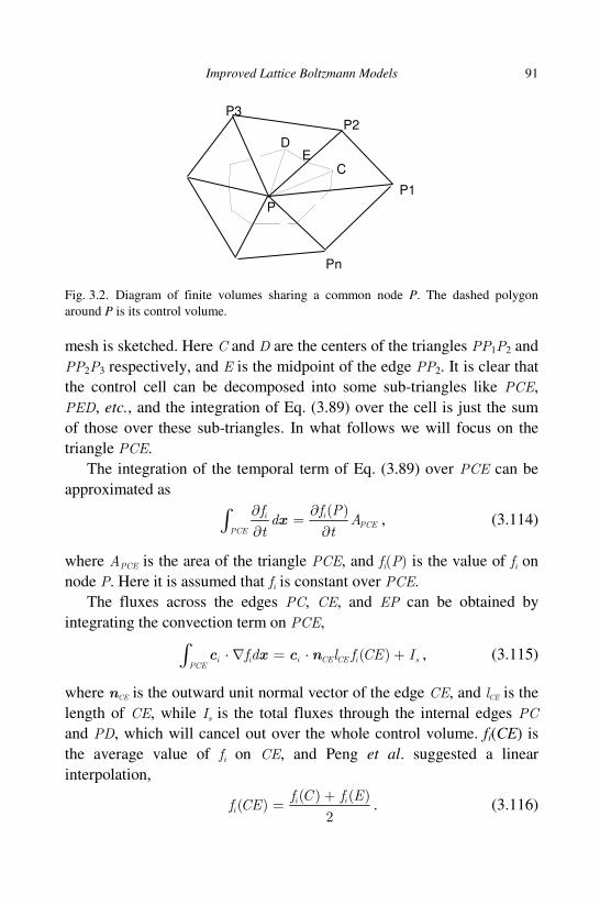
Improved Lattice Boltzmann Models 91
mesh is sketched. Here C and D are the centers of the triangles PP1P2 and
PP2P3 respectively, and E is the midpoint of the edge PP2. It is clear that
the control cell can be decomposed into some sub-triangles like PCE,
PED, etc., and the integration of Eq. (3.89) over the cell is just the sum
of those over these sub-triangles. In what follows we will focus on the
triangle PCE.
The integration of the temporal term of Eq. (3.89) over PCE can be
approximated as
( )ii
PCEPCE
f Pfd A
t t
∂∂=
∂ ∂∫ x , (3.114)
where APCE is the area of the triangle PCE, and fi(P) is the value of fi on
node P. Here it is assumed that fi is constant over PCE.
The fluxes across the edges PC, CE, and EP can be obtained by
integrating the convection term on PCE,
( )i i i CE CE i sPCE
f d l f CE I∇ = ⋅⋅ +∫ nc x c , (3.115)
where nCE is the outward unit normal vector of the edge CE, and lCE is the
length of CE, while Is is the total fluxes through the internal edges PC
and PD, which will cancel out over the whole control volume. fi(CE) is
the average value of fi on CE, and Peng et al. suggested a linear
interpolation,
( ) ( )
( )2
i ii
f C f Ef CE
+= . (3.116)
P
P1
P2
Pn
C
E
D
P3
Fig. 3.2. Diagram of finite volumes sharing a common node P. The dashed polygon
around P is its control volume.
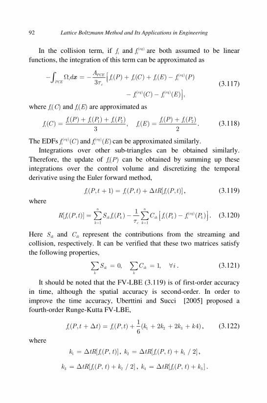
92 Lattice Boltzmann Method and Its Applications in Engineering
In the collision term, if fi and ( )eqif are both assumed to be linear
functions, the integration of this term can be approximated as
( )
( ) ( )
( ) ( ) ( ) ( )3
( ) ( ) ,
eqPCEi i i i i
PCEc
eq eqi i
Ad f P f C f E f P
f C f E
τ− Ω = − + + −
− −
∫ x (3.117)
where fi(C) and fi(E) are approximated as
1 2 2( ) ( ) ( ) ( ) ( )( ) , ( )
3 2
i i i i ii i
f P f P f P f P f Pf C f E
+ + += = . (3.118)
The EDFs ( )( )eqif C and ( )( )eq
if E can be approximated similarly.
Integrations over other sub-triangles can be obtained similarly.
Therefore, the update of fi(P) can be obtained by summing up these
integrations over the control volume and discretizing the temporal
derivative using the Euler forward method,
( , 1) ( , ) [ ( , )]i i if P t f P t tR f P t+ = + ∆ , (3.119)
where
( )
1 1
1[ ( , )] ( ) ( ) ( )
n neq
i ik i k ik i k i k
k kc
R f P t S f P C f P f Pτ= =
= − − ∑ ∑ . (3.120)
Here Sik and Cik represent the contributions from the streaming and
collision, respectively. It can be verified that these two matrices satisfy
the following properties,
0, 1,ik ik
k k
S C i= = ∀∑ ∑ . (3.121)
It should be noted that the FV-LBE (3.119) is of first-order accuracy
in time, although the spatial accuracy is second-order. In order to
improve the time accuracy, Uberttini and Succi [2005] proposed a
fourth-order Runge-Kutta FV-LBE,
1 2 3
1( , ) ( , ) ( 2 2 4)
6i if P t t f P t k k k k+ ∆ = + + + + , (3.122)
where
1 [ ( , )]ik tR f P t= ∆ , 2 1[ ( , ) / 2]ik tR f P t k= ∆ + ,
3 2[ ( , ) / 2]ik tR f P t k= ∆ + , 4 3[ ( , ) ]ik tR f P t k= ∆ + .

Improved Lattice Boltzmann Models 93
On the other hand, Stiebler et al. [2006] proposed a least-square-linear-
reconstruction (LSLR) method in evaluating the numerical flux after
noticing that the approximations in Eqs. (3.116) and (3.118) may lead to
some numerical instability. They assume that the distribution function is
linear in the cell around node P,
( ) ( ) ( )i i Pf f P= + − ⋅x x x G , (3.123)
where G(P) = ∇fi(P), which is obtained by solving the following
minimization problem,
2
( )1
min ) ( ) (( )k
n
k i i P PP
k
kw f f PP=
− − − ⋅ ∑G
x x G , (3.124)
where 2kk P Pw −−x x=‖ ‖ . After obtaining the solution by solving a linear
algebra system, the average value of fi on the edge CE can be
approximated by
11
( ) ( ) , 0,2
( )
( ) ( ) , otherwise.2
C Ei P i CE
i
C Ei P
xf P P
f CEx
f P P
+ + ⋅ − ⋅ > = + + ⋅ −
xG x c n
xG x
Recently, Patila and Lakshmisha [2009] further introduced the total
variation diminishing (TVD) approach in evaluating the numerical flux,
and Rossi et al. [2005] and Succi and Ubertini and Succi [2006] have
made some theoretical discussions about several fundamental issues of
FV-LBE, such as temporal and spatial accuracy and boundary conditions.
3.3.5 Finite-element based LBE methods
The finite-element method has also been used to solve the DVM (3.89).
Lee and Lin [2001] made the first contribution toward this direction
when they proposed their characteristic Galerkin (CG) FE-LBE. First,
integrating Eq. (3.89) along the characteristic line leads to
− −1 1 1 1( ), ( ), = (1 ) (( ) ( ) ( ), ( )+ ,() )i n n i n n i n n i n nf t t f t t q t t t q t t t+ + + +∆ Ω ∆ Ωx x x x ,
(3.125)
where ( )tx is the trajectory of the particle moving with velocity ci
,
0 ≤ q ≤ 1 is a free parameter. The terms on the right hand-side are the
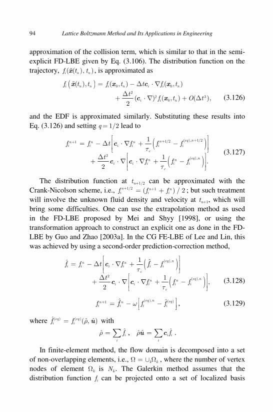
94 Lattice Boltzmann Method and Its Applications in Engineering
approximation of the collision term, which is similar to that in the semi-
explicit FD-LBE given by Eq. (3.106). The distribution function on the
trajectory, ( ( ), )i n nf t tx , is approximated as
( ) 0 0
22 3
0
( ), ( , ) ( , )
( ) ( , ) ( ),2
i n n i n i i n
i i n
f t t f t t f t
tf t O t
⋅
⋅
= − ∆ ∇
∆+ ∇ + ∆
x x c x
c x
(3.126)
and the EDF is approximated similarly. Substituting these results into
Eq. (3.126) and setting q = 1/2 lead to
( )
( )
( ), 1/21/21
2( ),
1
1.
2
eq nnn n ni i i i i i
c
eq nn ni i i i i
c
f f t f f f
tf f f
τ
τ
+++ = − ∆ ∇ + −
⋅
∆ + ⋅ ∇ ⋅ ∇ + −
c c
c
(3.127)
The distribution function at tn+1/2 can be approximated with the
Crank-Nicolson scheme, i.e., 1/2 1( ) / 2n n ni i if f f+ += + ; but such treatment
will involve the unknown fluid density and velocity at tn+1, which will
bring some difficulties. One can use the extrapolation method as used
in the FD-LBE proposed by Mei and Shyy [1998], or using the
transformation approach to construct an explicit one as done in the FD-
LBE by Guo and Zhao [2003a]. In the CG FE-LBE of Lee and Lin, this
was achieved by using a second-order prediction-correction method,
( )
( )
( ),
2( ),
1ˆ
1,
2
ˆ eq nn ni i i i i i
c
eq nn ni i i i i
c
f f t f f
tf f f
fτ
τ
− ∆ ⋅ ∇ + −
∆ + ⋅ ∇ ⋅ ∇ + −
=
c
c c
(3.128)
( ), ( )1 ˆˆ eq n eqn n
i i i if f ff ω+ = − − , (3.129)
where ( ) ( )ˆ ˆˆ( , )eq eqi if f ρ= u with
ˆˆ i
i
fρ = ∑ , ˆˆˆ i
i
ifρ = ∑u c .
In finite-element method, the flow domain is decomposed into a set
of non-overlapping elements, i.e., Ω = ∪kΩk , where the number of vertex
nodes of element Ωk is Nk.. The Galerkin method assumes that the
distribution function fi can be projected onto a set of localized basis

Improved Lattice Boltzmann Models 95
functions which are generally piecewise polynomials associated with the
elements,
1
( , ) ( ) ( ) ,kN
hi il kl i k
l
f t f t φ=
= ≡ ∈ Ω⋅∑ kx x xf φ , (3.130)
where φkl (l = 1, 2, …, Nk) are the basis functions on Ωk and fi1 is the
distribution function at the l-th node of Ωk. Substituting hif into Eqs. (3.128)
and (3.129), and multiplying the equations by φkl as a test function, and
then integrating over the element Ωk , we can obtain the CG FE-LBE,
( ) ( )
( )
( ),
( ),2
ˆ
,
ˆ eq nn n ni i i i i i
c
eq nn ni i i i i
t
t
τ
− = −∆ + −
+ ∆ + −
MM f f C f f
D f Q f f
f
(3.131)
( ), ( ),1 ˆ ˆ eq n eq nn ni i i iω+ = + − f f ff , (3.132)
where M, Ci , Di , and Qi are Nk ×Nk matrices,
21, , , , ( ) ,
21
, ( .)
,mn km kn imn km i kn imn km i kn
imn km i kn
c
M C D
Q
φ φ φ φ φ φ
φ φτ
= ⋅ = − ⋅ ∇
= − ⋅
=
∇
c c
c
Here the inner product is defined by ,f g fgd⟨ ⟩ = ∫ x . Equations (3.131)
and (3.132) constitute the basic process of the CG FE-LBE by Lee and
Lin [2001]. Based on the similar strategy, Min and Lee [2011] developed
a spectral-element discontinuous Galerkin (SEDG) method for solving
the DVM (3.89). Several other FE-LBE methods based on SEDG were
also proposed by independent groups [Shi et al., 2003; Düster et al.,
2006].
Another kind of FE-LBE was developed by Li et al. [2004] based on
the least-squares finite-element (LSFE) method, in which the time
evolution of DVM (3.89) is first discretized as
1
1 1(1 ) (1 )n ni i n n n n
i i i i i
f fqf q f q q
t
++ +− + ∇ + − = Ω + − Ω⋅ ∆
c , (3.133)
where q is again a parameter like that used in the FD-LBE and FV-LBE.
Obviously, Equation (3.133) reduces to the Crank-Nicolson scheme as
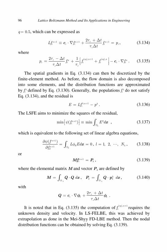
96 Lattice Boltzmann Method and Its Applications in Engineering
q = 0.5, which can be expressed as
1 1 12 cn n ni i i i i
c
tLf f f p
t
τ
τ+ + ++ ∆
≡ ⋅ ∇ + =∆
c , (3.134)
where
( ), 1 ( ),2 1 eq n eq nc n n
i i i i i i
c c
tp f f f f
t
τ
τ τ
+− ∆ = + + − ⋅ ∇ ∆c . (3.135)
The spatial gradients in Eq. (3.134) can then be discretized by the
finite-element method. As before, the flow domain is also decomposed
into some elements, and the distribution functions are approximated
by hif defined by Eq. (3.130). Generally, the populations h
if do not satisfy
Eq. (3.134), and the residual is
, 1h n hiE Lf p+= − . (3.136)
The LSFE aims to minimize the squares of the residual,
1 2min ( ) mink
nif E dψ
Ω
+ ≡ ∫ x , (3.137)
which is equivalent to the following set of linear algebra equations,
1
1
( )0
k
n
klnil
fL Ed
f
ψφ
Ω
+
+
∂= =
∂ ∫ x , 1, 2, , kl N= , (3.138)
or
1k
ni
+ =M Pf , (3.139)
where the elemental matrix M and vector Pk are defined by
k
dΩ
= ⋅∫M Q Q x , k
hkk d
Ω⋅= ∫P Q p x , (3.140)
with
2 c
i k k
c
t
t
τ
τ
+ ∆= ⋅ ∇ +
∆Q c φ φ .
It is noted that in Eq. (3.135) the computation of( ), 1eq n
if+
requires the
unknown density and velocity. In LS-FELBE, this was achieved by
extrapolation as done in the Mei-Shyy FD-LBE method. Then the nodal
distribution functions can be obtained by solving Eq. (3.139).

Improved Lattice Boltzmann Models 97
3.3.6 Taylor series expansion and least square based methods
In this part, we will introduce a new version of LBE (refereed to as
TLLBE) with nonuniform meshes, which was developed by Shu and his
coworkers [Chew et al., 2002; Niu et al., 2003; Shu et al., 2001; Shu
et al., 2002]. This method is based on the conventional LBE, the well-
known Taylor series expansion, the idea of developing Runge-Kutta
method, and the least squares approach. The final form of the method is
an algebraic formulation, in which the coefficients only depend on the
coordinates of mesh points and lattice velocity and can be computed in
advance. Furthermore, the method is also free of lattice models.
Taylor series expansion-based method
Without loss of generality, we consider a two-dimensional (2D) case. As
shown in Fig. 3.3, point A represents the grid point (xA, yA) at time t, and
A′ represents the position (xA + cixδt, yA + ciyδt) at time t + δt, and P
represents the position (xP, yP) with xp = xA + δx and yp = yA + δy. The
LBE gives that
( )1( , ) ( , ) ( , ) ( , )eqi t i i if A t f A t f A t f A tδ
τ ′ + = − − . (3.141)
For general cases, A′ may not coincide with the mesh point P. We first
consider the Taylor series expansion with truncation to the first order
derivative terms. Then, ( , )i tf A t δ′ + can be approximated by the
corresponding function and its derivatives at the mesh point P as
P
A
B
C
D
E
A'
B'
C'
D'
P'
E'
Fig. 3.3. Configuration of particle movement along ci .

98 Lattice Boltzmann Method and Its Applications in Engineering
2 2
( , )( , ) ( , )
( , )( ) ,( ) ,
i ti t i t A
i tA A A
f P tf A t f P t x
x
f P ty O x y
y
δδ δ
δ
∂ +′ + = + + ∆∂
∂ + + ∆ + ∆ ∆ ∂
(3.142)
where A A ix t Px x c xδ∆ = + − , A A iy t Py y c yδ∆ = + − . Note that the above
approximation has a truncation error of second order. Substituting
equation (3.142) into equation (3.141) gives
( )
( , ) ( , )( , )
( , ) ( , )( , ) .
i t i ti t A A
eqi i
i
f P t f P tf P t x y
x y
f A t f A tf A t
δ δδ
τ
∂ + ∂ ++ + ∆ + ∆
∂ ∂
−= +
(3.143)
It is indicated that equation (3.143) is a first order differential
equation, which only involves two mesh points A and P. When a uniform
grid is used, ∆x = ∆y = 0, then Eq. (3.143) reduces to the standard LBE.
Solving equation (3.143) can provide the density distribution functions at
all of the mesh points. An explicit formulation to update the distribution
function was developed by Shu et al., which is inspired by the Runge-
Kutta method. As we know, the Runge-Kutta method is developed to
improve the Taylor series method in the solution of ordinary differential
equations (ODEs). Usually the Taylor series method involves evaluation
of different orders of derivatives to update the functional value at the
next time level. For a given ODE with a complicated expression,
this application is very difficult. To improve the Taylor series method,
the Runge-Kutta method evaluates the functional values at some
intermediate points and then combines them (through the Taylor series
expansion) to form a scheme with the same order of accuracy.
With this idea in mind, we now look at Eq. (3.143). Notice that the
distribution function and its derivatives at the mesh point P are all
unknowns at the time level t + δt . So Eq. (3.143) has three unknowns in
total. To solve for the three unknowns, three equations are required.
However, Eq. (3.143) provides only one equation, and two additional
equations should be provided to close the system. As shown in Fig. 3.3,
the particles with velocity ci at two mesh points P and B at time t will
stream to the new positions P ′ and B ′ at t + δt. The distribution functions

Improved Lattice Boltzmann Models 99
at these new positions can be computed through the standard LBE, which
are given below,
( )1( , ) ( , ) ( , ) ( , )eqi t i i if P t f P t f P t f P tδ
τ ′ + = − − , (3.144)
( )1( , ) ( , ) ( , ) ( , )eqi t i i if B t f B t f B t f B tδ
τ ′ + = − − . (3.145)
Using Taylor series expansion with truncation to the first order
derivative terms, ( , )i tf P t δ′ + and ( , )i tf B t δ′ + in the above equations can
be approximated by the function and its derivatives at the mesh point P.
As a result, Eqs. (3.144) and (3.145) reduce to
( )
( , ) ( , )( , )
( , ) ( , )( , ) ,
i t i ti t P P
eqi i
i
f P t f P tf P t x y
x y
f P t f P tf P t
δ δδ
τ
∂ + ∂ ++ + ∆ + ∆
∂ ∂−
= +
(3.146)
( )
( , ) ( , )( , )
( , ) ( , )( , ) ,
i t i ti t B B
eqi i
i
f P t f P tf P t x y
x y
f B t f B tf B t
δ δδ
τ
∂ + ∂ ++ + ∆ + ∆
∂ ∂−
= +
(3.147)
where P ix tx c δ∆ = , P iy ty c δ∆ = , B B ix t Px x c xδ∆ = + − , and B By y∆ =
iy t Pc yδ+ − .
Equations (3.143), (3.146), and (3.147) form a system to solve for the
three unknowns. The solution of this system gives
( , ) /i t Pf P t δ+ = ∆ ∆ , (3.148)
where
A B B A B P P B P A A Px y x y x y x y x y x y∆ = ∆ ∆ − ∆ ∆ + ∆ ∆ − ∆ ∆ + ∆ ∆ − ∆ ∆ ,
, ,
,
( ) ( )
( ) ,
P A B B A i P B P P B i A
P A A P i B
x y x y g x y x y g
x y x y g
∆ = ∆ ∆ − ∆ ∆ + ∆ ∆ − ∆ ∆+ ∆ ∆ − ∆ ∆
( )1, ( , ) ( , ) ( , )eqi J i i ig f J t f J t f J tτ− = + − , J = P, A, B.
It should be noted that ,i Pg , ,i Ag , and ,i Bg are actually the post-
collision state of the distribution functions fi at time t and the mesh point
P, A, and B, respectively. Equation (3.148) has the second order of

100 Lattice Boltzmann Method and Its Applications in Engineering
truncation error, which may introduce a large numerical diffusion. To
improve the accuracy of numerical computation, the Taylor series
expansion can be truncated to the second order derivative terms. For the
two-dimensional case, this expansion involves six unknowns, that is, one
distribution function at the time level t + δt , two first order derivatives,
and three second order derivatives. To solve for these unknowns, six
equations are required to close the system. This can be done by applying
the second order Taylor series expansion at 6 points. As shown in
Fig. 3.3, the particles at six mesh points P, A, B, C, D, E at t will stream
to positions P ′, A′, B ′, C ′, D ′, E ′ at t + δt.. The distribution functions at
these new positions can be computed through the standard LBE. Then by
using the second order Taylor series expansion at these new positions in
terms of the distribution function and its derivatives at the mesh point P,
we can obtain the following equation system
6
: : : , :
1
Ti k i k i i k j i j
j
g s V s V=
= = ∑ , , , , , ,i P A B C D E= , (3.149)
where
( )( ): ( , , ) ( , , ) ( , , )
1k k k k k k
eqi k i x y t i x y t i x y tg f f f
τ= + − ,
2 2
:
( ) ( ) 1, , , , ,
2 2
k kTi k k k k k
x ys x y x y
∆ ∆ = ∆ ∆ ∆ ∆ ,
2 2 2
2 2 , , , , ,
T
i i i i ii i
f f f f fV f
x y x y x y
∂ ∂ ∂ ∂ ∂ = ∂ ∂ ∂ ∂ ∂ ∂ .
Here :i kg is the post-collision state of the distribution function fi at the
k-th point and the time t, : Ti ks is a vector with six elements formed by
the coordinates of mesh points, iV is the vector of unknowns at the
mesh point P and time t + δt., which also has six elements, : ,i k js is the j-th
element of the vector : Ti ks and :i jV is the j-th element of the vector
iV . Our target is to find its first element :1 ( , )i i tV f P t δ= + . Equation
system (3.149) can be put into the following matrix form
[ ] i i iS V g= , (3.150)

Improved Lattice Boltzmann Models 101
where
, , , , , , , , , , , Ti i P i A i B i C i D i Eg g g g g g g= ,
: ,
2 2:
2 2:
2 2:
2 2:
:
:
[ ] [ ]
1 ( ) /2 ( ) /2
1 ( ) /2 ( ) /2
1 ( ) /2 ( ) /2
1 ( ) /2 ( ) /2
1
i j
TP P P P P P P
TA A A A A A A
Ti B B B B B B B
Ti C C C C C C C
Ti D
Ti E
S s
s x y x y x y
s x y x y x y
s x y x y x y
s x y x y x y
s
s
α α
α
α
=
∆ ∆ ∆ ∆ ∆ ∆ ∆ ∆ ∆ ∆ ∆ ∆ ∆ ∆ ∆ ∆ ∆ ∆ = = ∆ ∆ ∆ ∆ ∆ ∆
2 2
2 2
( ) /2 ( ) /2
1 ( ) /2 ( ) /2
D D D D D D
E E E E E E
x y x y x y
x y x y x y
∆ ∆ ∆ ∆ ∆ ∆
∆ ∆ ∆ ∆ ∆ ∆
,
C C ix t Px x c xδ∆ = + − , C C iy t Py y c yδ∆ = + − ,
D D ix t Px x c xδ∆ = + − , D D iy t Py y c yδ∆ = + − ,
E E ix t Px x c xδ∆ = + − , E E iy t Py y c yδ∆ = + − .
The expressions of Px∆ , Py∆ , Ax∆ , Ay∆ , Bx∆ and By∆ have been
given previously. Since [Sα] is a 6×6 matrix, it is very difficult to obtain
an analytical expression for the solution of equation system (3.150), and
a numerical algorithm can be used to obtain an approximated solution.
Note that the matrix [Sα] only depends on the coordinates of the mesh
points, which can be computed once and stored for the application of
Eq. (3.150) at all time steps.
Improvement by least square method
In practical applications, it was found that the matrix [Sα] might be
singular or ill-conditioned. To overcome this difficulty and ensure that
the method is more general, Shu et al. [2002] suggested making use of
the least squares approach to optimize the approximation by Eq. (3.149).
This equation has 6 unknowns (elements of the vector Vα). If
Eq. (3.149) is applied at more than 6 mesh points, the system will be
over-determined. For this case, the unknown vector can be decided from
the least squares method. For simplicity, let the mesh point P be
represented by the index 0i = , and its adjacent points be represented by
index i = 1, 2, …, N, where N is the number of neighboring points
around P and it should be larger than 5. At each point, an error in terms
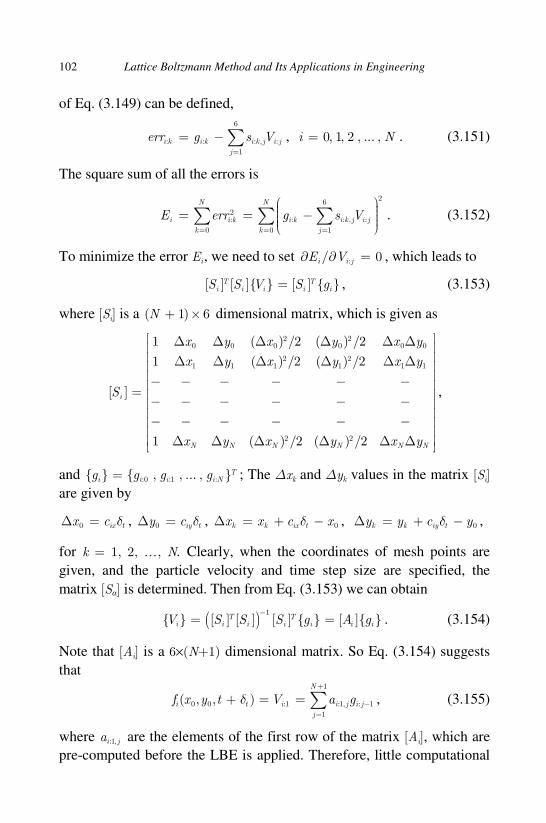
102 Lattice Boltzmann Method and Its Applications in Engineering
of Eq. (3.149) can be defined,
6
: : : , :
1
i k i k i k j i j
j
err g s V=
= − ∑ , 0, 1, 2 , ... ,i N= . (3.151)
The square sum of all the errors is
26
2: : : , :
0 0 1
N N
i i k i k i k j i j
k k j
E err g s V= = =
= = − ∑ ∑ ∑ . (3.152)
To minimize the error Ei , we need to set :/ 0i i jE V∂ ∂ = , which leads to
[ ] [ ] [ ] T Ti i i i iS S V S g= , (3.153)
where [Si] is a ( 1) 6N + × dimensional matrix, which is given as
2 20 0 0 0 0 0
2 21 1 1 1 1 1
2 2
1 ( ) /2 ( ) /2
1 ( ) /2 ( ) /2
[ ]
1 ( ) /2 ( ) /2
i
N N N N N N
x y x y x y
x y x y x y
S
x y x y x y
∆ ∆ ∆ ∆ ∆ ∆ ∆ ∆ ∆ ∆ ∆ ∆ − − − − − − = − − − − − − − − − − − −
∆ ∆ ∆ ∆ ∆ ∆
,
and :0 :1 : , , ... , Ti i i i Ng g g g= ; The ∆xk and ∆yk values in the matrix [Si]
are given by
0 ix tx c δ∆ = , 0 iy ty c δ∆ = , 0k k ix tx x c xδ∆ = + − , 0k k iy ty y c yδ∆ = + − ,
for k = 1, 2, …, N. Clearly, when the coordinates of mesh points are
given, and the particle velocity and time step size are specified, the
matrix [Sα] is determined. Then from Eq. (3.153) we can obtain
( ) 1 [ ] [ ] [ ] [ ] T T
i i i i i i iV S S S g A g−
= = . (3.154)
Note that [Ai] is a 6×(N+1) dimensional matrix. So Eq. (3.154) suggests
that
1
0 0 :1 :1, : 1
1
( , , )N
i t i i j i j
j
f x y t V a gδ+
−=
+ = = ∑ , (3.155)
where :1,i ja are the elements of the first row of the matrix [Ai], which are
pre-computed before the LBE is applied. Therefore, little computational

Improved Lattice Boltzmann Models 103
effort is introduced as compared with the standard LBE. Note that the
function g is evaluated at the time level t. So Eq. (3.155) is actually an
explicit form to update the distribution function at the time level t + δt .
In the above process, there is no requirement for the selection of
neighboring points, or in other words, Eq. (3.155) is independent from
the mesh structure, and we only need to know the coordinates of the
mesh points. Therefore Eq. (3.155) is basically a meshless form.
Theoretical analysis has shown that the above least square-based LBE
can recover the Navier-Stokes equations with second order of accuracy,
no matter whether the mesh is uniform or non-uniform. The TLLBE has
been successfully applied to a variety of flows with nonuniform meshes.
An example for the flow around a circular cylinder is shown in Fig. 3.4.
3.4 Accelerated LBE Methods for Steady Flows
Steady flows appear in many physical and engineering situations. As a
time-marching method, however, the LBE may encounter some
convergence difficulties when applied to steady flows. The slow
convergence rate is an inherent disadvantage of the standard LBE. As
shown previously, the LBE is an explicit time-marching method for
Fig. 3.4. Flow around a circular cylinder. Top: Computational mesh; Bottom: Streamline
with Re=20(left) and 40 (right).

104 Lattice Boltzmann Method and Its Applications in Engineering
compressible fluid flows with low Mach numbers, and can be viewed as
an explicit artificial compressibility scheme for incompressible Navier-
Stokes equations. In addition to the error due to numerical discretization,
the finite Mach number effect also introduces a grid independent
compressibility error. To reduce this error, the Mach number must be
kept sufficiently small. As the Mach number becomes smaller, however,
it would become increasingly computational expensive to solve the
compressible Navier-Stokes equations using the standard LBE [Lai et al.,
2001].
Some efforts have been made to accelerate the convergence rate of
the LBE from different viewpoints. In general, the existing accelerated
LBE models fall into two categories, i.e., time dependent methods and
time-independent methods. In the former, the LBE still evolves as a
time-marching process, but the evolution equation is altered. On the
other hand, in the time independent approach, a linear or nonlinear
algebra system derived from the time independent form of the steady
LBE or DVM is solved directly.
3.4.1 Spectrum analysis of the hydrodynamic equations of the
standard LBE
The convergence difficulty of LBE roots in the large disparity between
the acoustic wave speed and the fluid speed in low Mach number flows,
as in the classical CFD methods [Turkel, 1999]. Usually, for any explicit
scheme, the CFL condition should be fulfilled for the sake of numerical
stability. Therefore, the time step should be chosen such that it is
inversely proportional to the sound speed of the acoustic wave, during
which the waves driven by the fluid change slightly. As a result, a large
number of time steps are needed to reach the steady state of the flow. As
an explicit scheme, the LBE also suffers from this problem.
To see this more clearly, we now make a spectral analysis of
the hydrodynamic equations derived from standard LBGK models (see
Eqs. (1.69) and (1.70)). For two-dimensional flows, these equations can
be written in a vector form,
,vt x y
∂ ∂ ∂+ + =
∂ ∂ ∂Q E F
R Q (3.156)

Improved Lattice Boltzmann Models 105
where R represents the vector associated with the viscous terms, and
Q = (ρ, ρu, ρv)T, E = (ρu, ρu2 + cs2ρ, ρuv)T, F = (ρv, ρuv, ρv2 + cs
2ρ)T,
where u and v are the x- and y- components of the fluid velocity u,
respectively. Equation (3.156) can be further written as
,vt x y
∂ ∂ ∂+ + =
∂ ∂ ∂Q Q Q
A B R Q (3.157)
where
2 2
0 1 0
2 0sc u u
uv v u
∂ = = − ∂ −
EA
Q,
2 2
0 0 1
0 2s
uv v u
c v v
∂ = = − ∂ −
FB
Q. (3.158)
It can be easily shown that the eigenvalues of the matrices A and B
are respectively
( ) , su u cλ = ±A , ( ) , sv v cλ = ±B . (3.159)
Therefore, the condition number of A is
,
( ) 1( ) max 1
( )
i
i jj M
λκ
λ
= +
AA
A∼ , (3.160)
where M is the Mach number. The condition number of matrix B is
similar. Therefore, κ(A) and κ(B) will be very large as the Mach number
of the flow is small, which means that the waves in the fluid transfer with
quite different speeds, and this will make the LBE converge very slowly.
It is noted the viscous terms also have complex influences on the wave
speeds, depending on the Reynolds number and the ratio of the Reynolds
number to the Mach number, and the convergence difficulty can be
further exacerbated by the magnitude of the diffusion terms [Lee, 1996].
3.4.2 Time-independent methods
At steady state, the standard LBGK equation with a body force F can be
written as
( )( ) ( ) ( ) (1
)eqi i t i i i t if ff Ffδ δ
τ + − = − − + x c x x x , 0 1i b= −∼ . (3.161)

106 Lattice Boltzmann Method and Its Applications in Engineering
This equation can also be rewritten in matrix formulation,
( ) ( ) t⋅ + ′⋅ =K fS x Ff x δ , (3.162)
where S and K are the local streaming and collision matrices,
respectively, which are defined by [Bernaschi et al., 2002; Bernaschi and
Succi, 2003],
0 0 1 0 1 0( ) ( ), ( ), , ( )T
t t b tf f fδ δ δ− ⋅ = + + + S f x x c x c x c ,
2
2 4
( )11
2
i j i i s a jiij ij
s s
c c c c c c uK
c c
α α α β β α βδωδτ τ
− = − + + ,
while F′ is a vector consisting of the forcing terms, 0 1 1[ , , , ]TbF F F −′ =F .
For a lattice with N nodes, Eq. (3.162) represents a nonlinear algebraic
system of the form
[ ][ ] [ ]A f F= , (3.163)
where [A] is a bN × bN block matrix consisting of S and K, [f] and [F]
are two vectors with bN elements. This nonlinear system can be solved
iteratively. For example, Bernaschi et al. [2002, 2003] suggested a
Newton-Raphson procedure to linearize Eq. (3.163), which is then solved
by a generalized method of residuals (GMRES). However, it was found
that the convergence of this method may be rather slow for high-
Reynolds number flows. In order to release this difficulty, a viscosity
annealing technique was introduced into the iterative process [Bernaschi
and Succi, 2003]. This is achieved by letting the relaxation time change
with the iteration, i.e.,
1
1 1k
k k+
= + ατ τ
, k = 0, 1, …,
where αk is the annealing increments at the k-th iteration. This annealing
technique makes the iteration process start with a low Reynolds number
and attain the desired one at the final state.
For Stokes flows with a low Reynolds number, the matrix
formulation of the steady LBE (3.162) can be simplified. In this case, the
nonlinear terms in the fluid velocity in the EDF can be neglected, i.e.,

Improved Lattice Boltzmann Models 107
( )
21eq i
i i
s
fc
ω ρ ⋅ = +
c u. (3.164)
If the relaxation time is set to be 1.0, the steady LBE becomes,
(
2
) 1( ) ( )i j
ieq
i i t i t i
s
j t i
j
f F ff Fc
ωδ δ δ+ ⋅ +
= + = +∑c c
x c x . (3.165)
With the relation between the conserved quantities m = (ρ, ρu), the
above formulation can be further written as a linear system of these
variables [Verberg and Ladd, 1999],
[ ][ ] [ ]A m B= , (3.166)
where [A] = I – PTE and [B] = PTF, with P being a (D + 1)N × bN
block-diagonal matrix, P = diag(p, p, …, p), pi = (1, ci)T, T is a bN ×
bN transition matrix, and E = diag(e, e, …, e), with ei = (ω i, ω i ci / cs2)T.
A biconjugate gradient algorithm was proposed to solve the above
algebra system [Verberg and Ladd, 1999].
It was found that with the matrix formulation, the accelerated LBE
methods could be 1∼2 orders of magnitude faster than the standard one
[Bernaschi et al., 2002; Bernaschi and Succi, 2003; Verberg and Ladd,
1999; Noble and Holdych, 2007]. Some methods were also developed to
solve the steady discrete velocity model (3.89) directly using certain
finite-difference schemes. For instance, Tölke et al. [2002] proposed an
implicit second-order finite difference scheme, and introduced a
nonlinear multigrid method to solve the nonlinear algebra system.
3.4.3 Time-dependent methods
Some time-independent acceleration techniques have also been
introduced to improve the convergence of LBE for steady flows. The
most straightforward way is employing certain implicit schemes to
discretize the time-dependent equation (3.89) so that a larger time step
can be used [Lee and Lin, 2003; Seta and Takahashi, 2002; Tölke et al.,
1998]. On the other hand, Mavriplis [2006] developed a multigrid
technique which makes use of the non-linear LBE time-stepping scheme
on each grid level. Although all these schemes can improve the

108 Lattice Boltzmann Method and Its Applications in Engineering
convergence rates, their formulation and implementation are much more
complicated than the standard LBE.
Motivated by the precondition method for solving the compressible
Navier-Stokes equations, Guo et al. [2004] developed a time-independent
preconditioned LBE (PLBE) with the same structure as the standard one.
The evolution equation of PLBE without considering the influence of
body forces is
( )( , ) ( , ; )1
( , ) ( , ) eqi i t t i i i
p
tf t f t f f γδτ
ρδ + + − = − − x xx uc , (3.167)
where τp is a relaxation time to be determined, and the modified EDF
contains an adjustable parameter γ,
( )2
( )
2 41
2
: seqi i
s
i ii
s
cf
c cω ρ
γ
− = + +
⋅
uu c c Ic u. (3.168)
The fluid density and velocity in the PLBE are defined as those in the
standard LBE. Through the Chapman-Enskog procedure, we can derive
the macroscopic equations from the LBE (3.167) as
( ) 0t
ρρ
∂+ ∇ ⋅ =
∂u , (3.169)
( ) υ*
( ) 1 1 1( )p
t
ρρ ρ
γ γ γ
∂+ ∇ ⋅ = − ∇ + ∇ ⋅
∂u
uu S , (3.170)
where * 2
sp cγ ρ= , and 2( 0.5)s p tcν γ τ δ= − . It is clear that for steady
flows, Eqs. (3.169) and (3.170) are identical to those derived from the
standard LBE except for a different equation of state. It is clear that the
effective sound speed * */s sc p cρ γ= ∂ ∂ = is decreased as γ < 1.
In the presence of a body force F, the PLBE (3.167) should be
modified by adding a forcing term δtFi on its the right hand side. The
forcing term can be taken as those described in Sec. 3.2, but with a body
force scaled by γ. For instance, the scaled LGA forcing scheme can be
expressed as 2/i i siF cω γ⋅= c F . With this forcing term, the resultant
momentum equation takes the same form as Eq. (3.170) but with a scaled
body force /γF .

Improved Lattice Boltzmann Models 109
The macroscopic equations (3.169) and (3.170) can be interpreted as
preconditioned Navier-Stokes equations. In fact, the vector form of this
system is
vt x y
∂ ∂ ∂+ + =
∂ ∂ ∂Q Q Q
PA PB PR Q , (3.171)
where Q, A, B, and R are the same as defined earlier except that cs is
replaced by the effective sound speed *sc . The matrix 1 1diag(1, , )γ γ− −=P
is a preconditioner. It can be shown that the eigenvalues of the pre-
conditioned convection matrix PA are now,
1
( ) ( , )su u cλγ
= ±PA , (3.172)
where
2 2)(1 ) (s sc u cγ γ= − + (3.173)
is an effective sound speed. It is clear that sc reduces to the original sound
speed cs as γ = 1. Conversely, as γ approaches to zero, sc approaches to
the fluid speed u. Therefore, one can decrease the disparity between the
speeds of the acoustic wave and the waves propagating with the fluid
velocity by adjusting this parameter, and thus accelerate the convergence
rate of the LBE. It is also noted that for low Mach number flows as
u → 0, we have *s s sc c cγ= = .
According to the effective sound speed *sc , one can define an effective
Mach number *M as
* *0 / sM U c= . It is clear that
*M M Mγ= ≤ as
0 < γ ≤ 1. In practical applications, the parameter γ can be chosen such
that M * is low enough for a given flow condition. This can be done by
first specifying the value of M * according to the flow condition and then
setting * 2( / )M M=γ .
The parameter γ will influence on the numerical stability of the PLBE.
In fact, from the relationship between the viscosity and the relaxation
time, one can obtain that
3
0.5Re
p
NMτ
γ− = , (3.174)
which indicates that the value of τp – 0.5 increases with decreasing γ for
a given M and Re on a fixed lattice. Therefore, it is expected that the

110 Lattice Boltzmann Method and Its Applications in Engineering
PLBE (3.167) has a better numerical stability range than the standard
one for small Mach number or high Reynolds number flows. It is also
noted that γ can also influence the EDF ( )eqif . The decrease in γ means an
increase in the last term in the brackets of the EDF given by Eq. (3.168),
which may make the EDF become negative, and thus cause numerical
instability. These arguments indicate that the parameter γ have
complicated influences on the numerical stability of the PLBE.
The stability of the PLBE can be analyzed using the von Neumann
linear analysis method. To do so, the distribution function ( , )if tx is first
expanded around a constant global EDF (0)if ,
(0)0 0( ( , ), ) ( , )i i if t f f tρ ′= + xux , (3.175)
where ρ0 and u0 are the constant density and velocity, respectively,
and ( , )if t′x is the fluctuation of fi around (0)if . With this expansion, the
linearized PLBE reads
1
( , ) ( , ) ( , ) ( , ) ,i i t t i i ij j
p
f t f t f t G f tδ δτ
′ ′ ′ ′+ + − = − − x c x x x (3.176)
where
( )
0 0( , )eqi
ij
j
fG
f
ρ∂=
∂u
is the Jacobian matrix evaluated at the uniform mean density and
velocity. It is noted that G does not vary in space or time. Equation
(3.176) can be rewritten in a compact form as
( , ) ( , )i i t t ij jf t M f tδ δ′ ′+ + =x c x , (3.177)
where the matrix M is defined by
1 1
1ij ij ij
p p
M Gδτ τ
= − + .
The Fourier transform of Eq. (3.177) gives that
( , ) exp[ i ] ( , )i t i ij jF t M F tδ+ = − ⋅k k e k , (3.178)
where i 1= − , ( , )jF tk is the Fourier transform of ( , )if t′x , k is the wave
number in units of 1/δx , and ei = ci/c is the dimensionless discrete

Improved Lattice Boltzmann Models 111
velocity. The spatial dependence of the stability of the PLBE is
determined by the eigenvalues of the matrix Γ,
( ) exp[ i ]ij i ijMΓ = − ⋅k k e .
For the D2Q9 model, the explicit expression of the Jacobian matrix G
can be written as
20 0
20 0
31 3( ) 2( )
2
92( ( ) ( )
2) ,
ij i i j j
i i j i
G ωγ
γ
= ⋅ ⋅ ′ ′+ − −
′ ′+
⋅ ⋅ ⋅
−
e e e u u
e u e e e u
(3.179)
where 0 0/c′ =u u . It can be shown that the eigenvalues of G are 1 and 0
with multiplicities 3 and 6, respectively, which are independent of γ and
0′u . Accordingly, the eigenvalues of the matrix M are 1 and 1−1/τp .
It is clear that Γ = M as k = 0, therefore the PLBE (3.167) is
asymptotically stable if |1 − 1/τp | < 1, i.e. τp > 0.5, which is the same as
the standard LBE. As k ≠ 0, the eigenvalues of Γ has a complex
dependence on the parameters γ , 0′u , k, and τp, and hence it is rather
difficult to give a complete mapping of all the stability boundaries.
Guo et al. have made an analysis in a special case, i.e. both the wave
number κ and the uniform velocity u0 are aligned with e1. In Fig. 3.5 the
Fig. 3.5. The modulus of ΓΓΓΓ vs τs and u0′ for different γ (Guo et al., Phys. Rev. E 70,
066706, 2004).

112 Lattice Boltzmann Method and Its Applications in Engineering
modulus of the matrix Γ, i.e., the maximum magnitude of the
eigenvalues, are shown as a function of 0′u and the relaxation time τs ,
which corresponds to the standard LBE and is related to τp by
0.5 ( 0.5)s pτ γ τ= + − .
It is observed that for each value of γ, there exists a critical value of
the velocity, uc , above which the modulus of Γ increases dramatically,
meaning that the PLBE would become unstable. This critical value
clearly depends on the parameter γ : the smaller the γ, the lower the uc. It
indicates that the stable range of PLBE is reduced as compared to the
standard LBE. Fortunately, for small Mach number flows when LBE
works, the fluid velocity is usually much lower than uc, and under such a
circumstance the PLBE is expected to have a stability similar to the
standard LBE.
The PLBE has been shown to be able to accelerate the convergence
rate significantly by adjusting the control parameter γ. In Fig. 3.6, the
convergence processes of the PLBE and the standard LBE for the lid-
driven flow in a square cavity are presented at Re = 400 and 1000 (based
on the driven velocity and cavity height), respectively. It is clearly seen
Fig. 3.6. Time histories of PLBE and standard LBE for the cavity flow. M*=0.058. Lattice size: 257×257 (Guo et al., Phys. Rev. E 70, 066706, 2004).

Improved Lattice Boltzmann Models 113
that the PLBE enhanced the convergence rate greatly for both cases
compared with the standard LBE.
It should be emphasized that the acceleration of PLBE is achieved
without sacrificing the accuracy of the solution. In Fig. 3.7, the velocity
and pressure distributions along the vertical and horizontal lines through
the cavity center are presented for Re = 1000, together with the
benchmark results [Ghia et al., 1982; Botella and Peyret, 1998]. It is seen
that in all cases the velocity distributions predicted by the PLBE agree
well with the benchmark solutions, and the difference between these
results with different γ is nearly indistinguishable. However, some
prominent differences are observed among the pressure distributions for
different values of γ. The differences are small in the central region, but
become larger near the walls. Also, the differences increase as Re
becomes larger. The comparison shows that the pressure distributions
predicted by the PLBE with γ < 1 agree better with the benchmark
solutions [Botella and Peyret, 1998] than that by the standard LBE
(γ = 1), which demonstrates the desirable properties of PLBE.
Fig. 3.7. Velocity [(a) and (b)] and pressure [(c) and (d)] profiles through the cavity
center at Re =1000 (Guo et al., Phys. Rev. E 70, 066706, 2004).

114 Lattice Boltzmann Method and Its Applications in Engineering
It is noted that some oscillations occur during the convergence
process. This is due to the reflection of acoustic waves on the walls. Such
oscillations can be damped out by enhancing the bulk viscosity, which
does not alter the solutions for incompressible flow or compressible flow
with low Mach number. The suppression of such oscillations can further
accelerate the convergence process. This technique can be achieved
straightforwardly in MRT-LBE, and several such methods have been
developed recently by Izquierdo and Fueyo [2008, 2009].
3.5 Summary
This chapter has presented some improved LBE methods from different
viewpoints. Particularly, we have focused on the following five special
topics:
(i) LBE models with reduced compressibility errors. Because the
standard LBE simulates the compressible Navier-Stokes equations,
errors due to the compressibility will arise when applied to
incompressible flows. In order to reduce such errors, some
incompressible LBE models have been developed. For steady
incompressible flows, the models developed in [Zou et al., 1995;
Lin et al., 1996] can be employed, while for unsteady flows several
other more elaborated models [Chen and Ohashi, 1997; He and Luo,
1997; Guo et al., 2000] should be used.
(ii) LBE models with reduced compressibility errors. Because the
standard LBE simulates the compressible Navier-Stokes equations,
errors due to the compressibility will arise when applied to
incompressible flows. In order to reduce such errors, some
incompressible LBE models have been developed. For steady
incompressible flows, the models developed in [Zou et al., 1995;
Lin et al., 1996] can be employed, while for unsteady flows several
other more elaborated models [Chen and Ohashi, 1997; He and Luo,
1997; Guo et al., 2000] should be used.
(iii) Treatment of body force in LBE with reduced discrete effects. As
the fluid is exposed to a body force field, it is important to
incorporate its effect into LBE. Although a variety of methods have

Improved Lattice Boltzmann Models 115
been proposed, the analysis indicates that care must be taken when
implementing these methods because of the discrete lattice effects.
In this regard, the forcing schemes developed in [He et al., 1998]
and [Guo et al., 2002] are the most accurate methods, satisfying
certain necessary constraints required for reproducing the desired
body force in the hydrodynamic equations.
(iv) LBE methods with nonuniform grids. The use of a regular lattice as
the computational mesh limits the applications of the standard LBE
for flows with irregular geometries. One straightforward extension
of the standard LBE in this respect is to make use of grid-refinement
or multi-block techniques [Filippova and Hänel, 1998; Dupuis and
Chopard, 2003; Yu et al., 2002; Guo et al., 2003; Crouse et al.,
2003; Tölke et al., 2006; Yu and Fan, 2009]. Meanwhile, the
interpolation supplemented method [He et al., 1996] utilizes the fact
that the computational mesh can be decoupled from the underlying
discrete velocity set. It is noted that both of the above methods still
depend on the standard LBE. On the other hand, after recognizing
that the LBE can be viewed as a special finite-difference scheme of
the Boltzmann equation, some LBE methods using nonuniform
grids have been developed by discretizing the DVM using the finite-
difference, finite-volume, or finite-element methods. The Taylor
series expansion- and least square-based LBE method developed by
Shu et al. [2001] provides a meshless- like version.
(v) Accelerated LBE methods for steady flows. Because of the low
Mach number limitation, the standard LBE usually suffers from a
slow convergence rate for steady flows. In order to improve the
convergence, two types of techniques, i.e., time-independent and
time-dependent approaches, have been introduced into LBE. In
general, the time-independent methods involve a large scale linear
or nonlinear algebraic system which can be solved by iterative
algorithms. The solution procedure of such methods is quite
different from the standard LBE. On the other hand, the time-
dependent accelerated LBE is more resemble the standard LBE.
Particularly, the preconditioned LBE proposed by Guo et al. [2004]
has the same structure as and shares all of the advantages of the
standard one.

116 Lattice Boltzmann Method and Its Applications in Engineering
It should be pointed out that the improved methods listed in this
chapter can be combined with each other to improve the performance of
LBE further. For example, a nonuniform grid can be used in the PLBE,
and the convergence rate of LBE can also be accelerated by adding a
fictitious body force [Kandhai et al., 1999].

117
Chapter 4
Sample Applications of LBE for
Isothermal Flows
In the previous three chapters we have presented some standard and
improved LBE models for isothermal flows, and some methods to realize
certain prescribed initial and boundary conditions were also discussed.
With these basic ingredients, now we are ready to simulate some simple
isothermal flows. In this chapter we will first discuss the structure of
an LBE algorithm, and then present several sample applications to
demonstrate the implementation details and numerical results.
4.1 Algorithm Structure of LBE
The picture of the collision and streaming processes of LBE, in either
LBGK or MRT-LBE models, is rather clear, and it is straightforward to
implement both processes. Generally, an LBE algorithm can be designed
following two kinds of structures, i.e., collision-streaming fashion where
at each time step the collision is first executed and then the post-collision
distributions are shifted to their neighbors, and streaming-collision
fashion which exchanges the above procedure. It can be shown these two
algorithm structures are identical, and we will follow the former one in
this book. A typical flowchart of such LBE algorithm is shown in
Fig. 4.1, but it should be noted that the sequence of the subroutines can
be adjusted in some cases. In what follows the main subroutines of the
algorithm will be described. For clarity and simplicity, we will take the
D2Q9 model as an example, and the code will be written in ANSI-C
language. The global variables are defined in a header file D2Q9.h:

118 Lattice Boltzmann Method and Its Applications in Engineering
Fig. 4.1. Flowchart of LBE algorithm.
Collision
Streaming
Boundary Conditions
Fluid Variables
Stop Criterion
Reached ?
End
Yes
No
Simulation Parameters
Initialization
Tim
e m
arch
ing
pro
cess

Sample Applications of LBE for Isothermal Flows 119
//-----------------------------------------------
// ----- Header file of the D2Q9 model --
//-----------------------------------------------
//File name: D2Q9.h
#include <stdio.h>
#include <stdlib.h>
#include <math.h>
#define Nx 100 // number of cells in x-direction
#define Ny 100 // number of cells in y-direction
#define Nx1 (Nx+1)
#define Ny1 (Ny+1)
#define Q 9 // number of discrete velocities
#define rho0 1.0 // initial density
#define ux0 0.0
#define uy0 0.0 // (ux0, uy0) is the initial velocity
int cx[Q]=0, 1, 0, -1, 0, 1, -1, -1, 1;
int cy[Q]=0, 0, 1, 0, -1, 1, 1, -1, -1;
double f[Ny1][Nx1][Q]; //array of the distribution functions
double f_post[Ny1][Nx1][Q]; // array of the post-collision
// distribution functions
double rho[Ny1][Nx1], ux[Ny1][Nx1], uy[Ny1][Nx1];
// arrays of fluid density and velocity
double tau; // relaxation time for BGK model
double s[Q]; // relaxation rates for MRT model
double D[Q]=9, 36, 36, 6, 12, 6, 12, 4, 4; // D = M*MT
double w[Q]=4.0/9, 1.0/9, 1.0/9, 1.0/9, 1.0/9, 1.0/36,
1.0/36, 1.0/36, 1.0/36; // weights in EDF
int rc[Q]=0,3,4,1,2,7,8,5,6;
// index of the reversed velocity used in bounce-back scheme
//---------- end of header file------------------
Initialization
As described in Chapter 3, the distribution functions can be initialized
by either the equilibrium or non-equilibrium methods, or the more
elaborated iterative method. The following subroutine gives the
equilibrium initialization method.

120 Lattice Boltzmann Method and Its Applications in Engineering
//-------------------------------------------------------
//Subroutine: initialization with the equilibrium method
//-------------------------------------------------------
void Init_Eq()
int j, i, k;
for (j=0;j<=Ny;j++) for(i=0;i<=Nx;i++)
rho[j][i]=rho0;
ux[j][i]=ux0;
uy[j][i]=uy0;
for(k=0;k<Q;k++)
f[j][i][k]=feq(rho[j][i],ux[j][i],uy[j][i],k);
//-------------- end of initialization ----------
The calculation of the EDF is realized by the function feq():
//-----------------------------------------------
// Subroutine: calculation the equilibrium distribution
//-----------------------------------------------
double feq(double RHO, double U, double V, int k)
double cu, U2;
cu=cx[k]*U+cy[k]*V; // c_k*u
U2=U*U+V*V; // u*u;
return w[k]*RHO*(1+3*cu+4.5*cu*cu-1.5*U2);
//----------- end of equilibrium ---------------
The equilibrium method works well for steady flows. But it may
introduce some initial errors for unsteady flows. The nonequilibrium or
the iteration method [Mei et al., 2006] can give more accurate initial
values. Particularly, the latter can provide the compatible pressure as

Sample Applications of LBE for Isothermal Flows 121
well as the distribution functions. The codes for these methods can be
composed with similar structure, and will not be included in this book.
Collision
The subroutine for the BGK collision model is given below.
//-----------------------------------------------
// Subroutine: BGK collision
//-----------------------------------------------
void Coll_BGK()
int j, i, k;
double FEQ;
for(j=0;j<=Ny;j++) for(i=0;i<=Nx;i++)
for(k=0;k<Q;k++)
// the value of the EDF:
FEQ=feq(rho[j][i],ux[j][i],uy[j][i],k);
// the post-collision distribution function:
f_post[j][i][k]=f[j][i][k]-(f[j][i][k]-FEQ)/tau;
//---------------- end of BGK collision ---------
The collision process of MRT model contains three phases: (1)
transforming the distribution functions from velocity space to moment
space; (2) performing relaxation in moment space; (3) transforming the
moments back to the velocity space. With the transformation matrix
given in Chapter 1, the subroutine for the MRT collision model is
described as follows.
//-----------------------------------------------
// Subroutine: MRT collision
//-----------------------------------------------
void Coll_MRT()
int j, i, k;
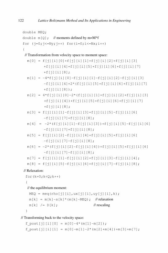
122 Lattice Boltzmann Method and Its Applications in Engineering
double MEQ;
double m[Q]; // moments defined by m=M*f
for (j=0;j<=Ny;j++) for(i=0;i<=Nx;i++)
// Transformation from velocity space to moment space:
m[0] = f[j][i][0]+f[j][i][1]+f[j][i][2]+f[j][i][3]
+f[j][i][4]+f[j][i][5]+f[j][i][6]+f[j][i][7]
+f[j][i][8];
m[1] = -4*f[j][i][0]-f[j][i][1]-f[j][i][2]-f[j][i][3]
-f[j][i][4]+2*(f[j][i][5]+f[j][i][6]+f[j][i][7]
+f[j][i][8]);
m[2] = 4*f[j][i][0]-2*(f[j][i][1]+f[j][i][2]+f[j][i][3]
+f[j][i][4])+f[j][i][5]+f[j][i][6]+f[j][i][7]
+f[j][i][8];
m[3] = f[j][i][1]-f[j][i][3]+f[j][i][5]-f[j][i][6]
-f[j][i][7]+f[j][i][8];
m[4] = -2*(f[j][i][1]-f[j][i][3])+f[j][i][5]-f[j][i][6]
-f[j][i][7]+f[j][i][8];
m[5] = f[j][i][2]-f[j][i][4]+f[j][i][5]+f[j][i][6]
-f[j][i][7]-f[j][i][8];
m[6] = -2*(f[j][i][2]-f[j][i][4])+f[j][i][5]+f[j][i][6]
-f[j][i][7]-f[j][i][8];
m[7] = f[j][i][1]-f[j][i][2]+f[j][i][3]-f[j][i][4];
m[8] = f[j][i][5]-f[j][i][6]+f[j][i][7]-f[j][i][8];
// Relaxation:
for(k=0;k<Q;k++)
// the equilibrium moment:
MEQ = meq(rho[j][i],ux[j][i],uy[j][i],k);
m[k] = m[k]-s[k]*(m[k]-MEQ); // relaxation
m[k] /= D[k]; // rescaling
// Transforming back to the velocity space:
f_post[j][i][0] = m[0]-4*(m[1]-m[2]);
f_post[j][i][1] = m[0]-m[1]-2*(m[2]+m[4])+m[3]+m[7];
Sample Applications of LBE for Isothermal Flows 123
f_post[j][i][2] = m[0]-m[1]-2*(m[2]+m[6])+m[5]-m[7];
f_post[j][i][3] = m[0]-m[1]-2*(m[2]-m[4])-m[3]+m[7];
f_post[j][i][4] = m[0]-m[1]-2*(m[2]-m[6])-m[5]-m[7];
f_post[j][i][5] = m[0]+m[1]+m[1]+m[2]+m[3]+m[4]+m[5]
+m[6]+m[8];
f_post[j][i][6] = m[0]+m[1]+m[1]+m[2]-m[3]-m[4]+m[5]
+m[6]-m[8];
f_post[j][i][7] = m[0]+m[1]+m[1]+m[2]-m[3]-m[4]-m[5]
-m[6]+m[8];
f_post[j][i][8] = m[0]+m[1]+m[1]+m[2]+m[3]+m[4]-m[5]
-m[6]-m[8];
//------------- end of MRT collision-------------
In the subroutine m[Q] is the moment array, and s[Q] is the
corresponding relaxation rates. D is a diagonal matrix relating to the
transformation matrix M, i.e. D=MMT. So, the inverse of M can be
simply expressed as 1 1T− −=M M D . meq() is the function of calculating
the equilibrium moments:
//-----------------------------------------------
// Subroutine: calculation the equilibrium moment
//-----------------------------------------------
double meq(double RHO, double U, double V, int k)
double x;
switch(k)
case 0: x=RHO; break;
case 1: x=RHO*(-2+3*(U*U+V*V)); break;
case 2: x=RHO*(1-3*(U*U+V*V)); break;
case 3: x=RHO*U; break;
case 4: x=-RHO*U; break;
case 5: x=RHO*V; break;
case 6: x=-RHO*V; break;

124 Lattice Boltzmann Method and Its Applications in Engineering
case 7: x=RHO*(U*U-V*V); break;
case 8: x=RHO*U*V; break;
default: x=0;
return x;
//----------- end of equilibrium moments --------
Streaming
The streaming process can be implemented straightforwardly.
Furthermore, certain boundary conditions such as the bounce-back
scheme can also be incorporated into this process. The subroutine reads,
//-----------------------------------------------
// Subroutine: Streaming
//-----------------------------------------------
void Streaming()
int j, i, jd, id, k;
for (j=0;j<=Ny;j++) for(i=0;i<=Nx;i++)
for(k=0;k<Q;k++)
jd=j-cy[k]; id=i-cx[k]; // upwind node
if(!boundary[jd][id]) // fluid node
f[j][i][k]=f_post[jd][id][k]; // streaming
else // boundary node
// bounce-back on the boundary node:
f[j][i][k]=f_post[jd][id][rc[k]]+6*w[k]*rho[j][i]*
(cx[k]*uwx[jd][id]+cy[k]*uwy[jd][id]);
//-----------------------------------------------
Here boundary[Ny1][Nx1] is a Boolean array that characterizes
the boundary nodes, and uw=(uwx, uwy) is the velocity of the

Sample Applications of LBE for Isothermal Flows 125
boundary node. Incorporating the bounce-back scheme into the
streaming process is efficient for flows with irregular boundaries such as
porous media. If only simple boundaries, such as flat walls, are involved,
the code can be improved by separating the boundary condition
treatments from the streaming process, and the flag boundary
[Ny1][Nx1] can be deleted in such case.
Boundary conditions
Assuming that the boundary is a flat wall located at y = 0, then for the
standard bounce-back scheme, the first layer of fluid nodes on the lattice
(j = 0) locates at y = δx ; For the half-way bounce-back scheme, the
location is at y = δx/2. For the modified bounce-back scheme, the non-
equilibrium extrapolation, and the hydrodynamic boundary conditions,
the location falls on the wall. As an example, in the following we will
give several subroutines to realize the boundary conditions of the Couette
flow confined between two parallel plates. The top plate moves with a
constant velocity u0 = (uw, 0), and the bottom plate is kept stationary.
Periodic boundary conditions are applied to the inlet and outlet.
The subroutine of the bounce-back rule is given as follows:
//-----------------------------------------------
// Subroutine: Bounce-back scheme
//-----------------------------------------------
void Bounce_back()
int i;
// j=0: bottom plate
for(i=0;i<=Nx;i++)
// bounce-back for particles hitting on the wall:
f[0][i][2]=f_post[0][i][4];
f[0][i][5]=f_post[0][i][7];
f[0][i][6]=f_post[0][i][8];
// j=Ny: top plate
for(i=0;i<=Nx;i++)
126 Lattice Boltzmann Method and Its Applications in Engineering
f[Ny][i][4]=f_post[Ny][i][4];
f[Ny][i][7]=f_post[Ny][i][5]+6*rho[Ny][i]*w[7]*cx[7]*uw;
f[Ny][i][8]=f_post[Ny][i][6]+6*rho[Ny][i]*w[8]*cx[8]*uw;
//-----------------------------------------------
The above bounce-back subroutine is executed after the collision
process. On the other hand, the modified bounce-back scheme should be
executed after the streaming process, and the collision is also performed
on the wall nodes. The subroutine reads as below:
//-----------------------------------------------
// Subroutine: Modified bounce-back scheme
//-----------------------------------------------
void M_bounce_back()
int i;
// j=0: bottom plate
for(i=0;i<=Nx;i++)
// bounce-back for particles hitting on the wall:
f[0][i][2]=f[0][i][4];
f[0][i][5]=f[0][i][7];
f[0][i][6]=f[0][i][8];
// j=Ny: top plate
for(i=0;i<=Nx;i++)
f[Ny][i][4]=f[Ny][i][2];
f[Ny][i][7]=f[Ny][i][5]+6*rho[Ny][i]*w[7]*cx[7]*uw;
f[Ny][i][8]=f[Ny][i][6]+6*rho[Ny][i]*w[8]*cx[8]*uw;
//-----------------------------------------------

Sample Applications of LBE for Isothermal Flows 127
Similarly, the non-equilibrium extrapolation scheme [Guo et al.,
2002a] is also executed after the streaming process. The subroutine of
this scheme is described below:
//-----------------------------------------------
// Subroutine: Non-equilibrium extrapolation
//-----------------------------------------------
void Noneq_BC()
int i, jd, id;
double FMf, FMb;
// j=0: bottom plate
for(i=0;i<=Nx;i++)
jd=1; id=i; // nearest neighboring fluid node
FMb=feq(rho[jd][id],0,0,2); // equilibrium at the boundary node
FMf=feq(rho[jd][id],ux[jd][id],uy[jd][id],2); // equilibrium
// at the fluid node
/*****
the extrapolation can also be taken from the nearest neighboring node along the
discrete velocity, i.e, jd=(Nx1+cy[2])%N1; id = (Nx1+i+cx[2])%Nx1;
*****/
// non-equilibrium extrapolation
f[0][i][2]=FMb+(f[jd][id][2]-FMf);
FMb=feq(rho[jd][id],0,0,5);
FMf=feq(rho[jd][id],ux[jd][id],uy[jd][id],5);
f[0][i][5]=FMb+(f[jd][id][5]-FMf);
FMb=feq(rho[jd][id],0,0,6);
FMf=feq(rho[jd][id],ux[jd][id],uy[jd][id],6);
f[0][i][6]=FMb+(f[jd][id][6]-FMf);
// j=Ny: top plate
for(i=0;i<=Nx;i++)
jd=Ny-1; id=i;
FMb=feq(rho[jd][id],u0,0,4);
128 Lattice Boltzmann Method and Its Applications in Engineering
FMf=feq(rho[jd][id],ux[jd][id],uy[jd][id],4);
f[Ny][i][4]=FMb+(f[jd][id][4]-FMf);
FMb=feq(rho[jd][id],u0,0,7);
FMf=feq(rho[jd][id],ux[jd][id],uy[jd][id],7);
f[Ny][i][7]=FMb+(f[jd][id][7]-FMf);
FMb=feq(rho[jd][id],u0,0,8);
FMf=feq(rho[jd][id],ux[jd][id],uy[jd][id],8);
f[Ny][i][8]=FMb+(f[jd][id][8]-FMf);
//-----------------------------------------------
Both the bounce-back schemes and the non-equilibrium extrapolation
method will introduce some approximation errors in the velocity
boundary conditions. On the other hand, the hydrodynamic scheme is
able to give the prescribed velocity exactly. The following subroutine
realizes the method developed by Zou et al. [1997]. Other hydrodynamic
schemes can be realized similarly.
//-----------------------------------------------
// Subroutine: Hydrodynamic scheme by Zou and He
//-----------------------------------------------
void Hydro_BC()
Int i;
double rhow;
// j=0: bottom plate
for(i=0;i<=Nx;i++)
// the density at wall node:
rhow = f[0][i][0]+f[0][i][1]+f[0][i][3]+2*(f[0][i][4]
+f[0][i][7]+f[0][i][8]);
f[0][i][2]=f[0][i][4];
f[0][i][5]=f[0][i][7]-0.5*(f[0][i][1]-f[0][i][3]);
f[0][i][6]=f[0][i][8]+0.5*(f[0][i][1]-f[0][i][3]);

Sample Applications of LBE for Isothermal Flows 129
// j=Ny: top plate
for(i=0;i<=Nx;i++)
// the density at wall node:
rhow = f[Ny][i][0]+f[Ny][i][1]+f[Ny][i][3]+2*(f[Ny][i][4]
+f[Ny][i][7]+f[Ny][i][8]);
f[Ny][i][4] = f[Ny][i][2];
f[Ny][i][7] = f[Ny][i][5]+0.5*(f[Ny][i][1]-f[Ny][i][3])
-0.5*rhow*u0;
f[Ny][i][8] = f[Ny][i][6]-0.5*(f[Ny][i][1]-f[Ny][i][3])
+0.5*rhow*u0;
//-----------------------------------------------
Fluid variables
The fluid variables, i.e., density and velocity, can be calculated from the
distribution functions directly. This is achieved by the subroutine
Den_Vel() given below.
//-----------------------------------------------
// Subroutine: Fluid density and velocity
//-----------------------------------------------
void Den_Vel()
int j, i;
for(j=0;j<=Ny;j++) for(i=0;i<=Nx;i++)
// density:
rho[j][i] = f[j][i][0]+f[j][i][1]+f[j][i][2]+f[j][i][3]
+f[j][i][4]+f[j][i][5]+f[j][i][6]+f[j][i][7]
+f[j][i][8];
ux[j][i] = (f[j][i][1]+f[j][i][5]+f[j][i][8]-f[j][i][3]
-f[j][i][6]-f[j][i][7])/rho[j][i];

130 Lattice Boltzmann Method and Its Applications in Engineering
uy[j][i] = (f[j][i][5]+f[j][i][6]+f[j][i][2]-f[j][i][7]
-f[j][i][8]-f[j][i][4])/rho[j][i];
//-----------------------------------------------
The above subroutines constitute the basic package for a typical LBE
algorithm. Of course, in practical applications these subroutines may be
modified to account for the particular situations. With a main() function
that controls the overall order of computations and operations, one can
design his own program for specific problems. Furthermore, the codes
listed above only provide a direct realization of the LBE method without
optimizations, and one can design more efficient algorithms and codes.
In the following sections we will demonstrate some sample applications
of LBE for incompressible flows.
4.2 Lid-Driven Cavity Flow
In this section we will simulate a two-dimensional steady flow in a
square cavity via the D2Q9 LBGK model. This problem is industrially
important and usually taken as one of the standard benchmark cases to
test computational schemes. The LBE was also applied to this problem
by many researchers. For example, Hou and Zou have performed some
detailed simulations [Hou and Zou, 1995]. The configuration of this
problem is shown in Fig. 4.2. The flow in the cavity is driven by the top
lid moving from left to right with a constant velocity u0. The flow is
characterized by the Reynolds number, Re = Lu0/ν, where L is the length
of the cavity and ν is the shear viscosity of the fluid. In the simulation, a
lattice with size of (N + 1) × (N + 1) is used, so that the lattice spacing is
/x L N=δ for the standard bounce-back, modified bounce-back, and the
non-equilibrium boundary conditions, while / ( 1)x L N= +δ for the
half-way bounce- back scheme.
For convenience, we will take the lattice spacing xδ , time increment
tδ , and lattice speed /x tc = δ δ , as the units of length, time, and velocity,
and assuming that the average density 0ρ is the density unit. As such, the

Sample Applications of LBE for Isothermal Flows 131
viscosity of the Navier-Stokes equations derived from the LBE model is
= c21
2sν τ −
, (4.1)
with 1/ 3sc = . In the literature, the simulated fluid with the above
viscosity is termed as lattice Boltzmann fluid (LBF) sometimes. The
Reynolds number of such fluid flows is then
= 0
2
3Re
( 0.5) 0.5s
Lu LM
c τ τ=
− −, (4.2)
where 0/ sM u c= is the Mach number. It should be born in mind that the
LBE is an artificial compressibility method for incompressible fluid
flows that has a vanishing Mach number. Provided the Mach number in
LBE is low enough (e.g. M < 0.3), the LBE results can serve as a good
approximation to the solutions of the incompressible Navier-Stokes
equations. Therefore, the Reynolds number is the only similitude
parameter between the LBE system and other fluid systems, while the
Mach number is not.
Fig. 4.2. Sketch of Lid-driven cavity flow.
ux = u0, uy = 0
ux = 0
uy = 0
ux = 0
uy = 0
ux = 0, uy = 0

132 Lattice Boltzmann Method and Its Applications in Engineering
According to the principle of similitude, one can obtain the
relationships between the variables of simulated physical system and
those of the LBE fluids:
L L=
x x,
0 0
t t
t t= ,
0 0
p p
p p= ,
0 0u u=
u u, (4.3)
with
20 0 0p uρ= , 2
0 0 0p uρ= , 0 0 0 0 ReL u L u
ν ν= = , (4.4)
where the variables with a bar represent the dimensional quantities of the
real system, while those without a bar are quantities in LBE. The
variables with a subscript “0” are characteristic quantities of the real and
LBE systems, respectively. With these relationships, one can calculate
the dimensional quantities of the real system from the LBE solutions.
In the simulations, the lattice size is taken to be 257×257, and the
driven velocity u0 is set to be 0.1. The relaxation time τ is determined
from the Reynolds number according to Eq. (4.2). The half way bounce-
back scheme is applied to the stationary and moving walls. An advantage
of this scheme is that no special treatment is required for the four corners.
It is noted that the top left and right corners are two singularities due to
the velocity difference of the side and top walls. We treat the corner
Fig. 4.3. Streamline of the cavity flow at Re=400 (left) and 1000 (right).

Sample Applications of LBE for Isothermal Flows 133
points as parts of the stationary walls in our simulations. The
convergence criterion is set to be
, 6
,
( , , 1000) ( , , )
10( , , 1000)
x y
x y
x y t x y t
ex y t
−
+ −
= <+
∑
∑
u u
u. (4.5)
Figure 4.3 shows the streamlines of the cavity flow at Re = 400 and
1000. It is seen that the fundamental characteristic of this flow is the
appearance of a large primary vortex in the center and two secondary
vortices near the two lower corners. These plots show clearly the effect
of the Reynolds number on the flow pattern. The velocity components, ux
and uy , along the vertical and horizontal center lines for different Re are
shown in Fig. 4.4, together with the results by Ghia et al. [1982]. It is
seen that the LBGK results agree well with the benchmark data. Recently,
a more careful comparative study on the computational performance of
several LBE models has been made [Luo et al., 2011].
The complete program for this test can be found in Appendix A.
4.3 Flow around a Fixed Circular Cylinder
Although the flow in the square cavity is complex, the geometry is
nevertheless simple since only flat boundaries are involved. In order to
demonstrate the performance of LBE for more general flows, we now
apply the LBE to the flow past a fixed circular cylinder. This flow has
been extensively studied both experimentally and numerically, and some
Fig. 4.4. Velocity profiles across the cavity center. Solid: LBGK results; Open circle:
data by Ghia et al. [1982].

134 Lattice Boltzmann Method and Its Applications in Engineering
applications of LBE based on uniform meshes [Guo et al., 2000;
Higuera and Succi, 1989; Wagner, 1994; Wagner and Hayot, 1995] or
nonuniform meshes [Filippova and Hänel, 1998; He and Doolen, 1997;
Mei and Shyy, 1998] have also been reported.
The D2Q9 LBGK model is again adopted in the simulations. The
flow domain and boundary conditions are sketched in Fig. 4.5. The
cylinder with a diameter D is put at 5D downstream from the entrance,
and the free-stream velocity U is set to be 0.1. Outflow condition is
imposed at the outlet, and free-slip boundary conditions are applied at the
two side boundaries. At the surface of the cylinder, no-slip boundary
condition is used. The Reynolds number of the flow is defined based on
the free-stream velocity and the cylinder diameter, Re = DU/ν. In the simulations, a lattice with size of Nx ×Ny = 401 × 201 is used.
The non-equilibrium extrapolation scheme for curved walls is used to
treat the no-slip boundary condition at the cylinder surface, and that for
flat walls is used to treat the inlet, outlet, and two side boundaries. The
velocity gradients in the boundary conditions are first discretized to
obtain the values of velocity at boundary nodes before implementing the
non-equilibrium extrapolation scheme.
Another important problem is the calculation of the force exerted by
the fluid on the cylinder. In classical CFD methods, this is usually done
by integrating the overall hydrodynamic forces along the surface,
p dAτ∂Ω = − + ⋅ ∫F I n , (4.6)
Fig. 4.5. Sketch of the flow around a circular cylinder.
5D
10D
ux = U , uy= 0
15D 5D
∑ux/∑y =0, uy = 0
∑ux/∑x = ∑uy/∑x = 0
∑ux/∑y =0, uy = 0

Sample Applications of LBE for Isothermal Flows 135
where n is the outward unit normal vector to the cylinder surface ∑Ω, and
( )T= ∇ + ∇u uτ ρν is the deviatoric stress tensor. Usually, the velocity
gradients in the above equation can be discretized as usual with certain
numerical schemes, as done by He and Luo [1997]. However, because
the stress is related to the second-order moments of the non-equilibrium
distribution functions, the calculation of the stress can be simplified in
LBE [Filippova and Hänel, 1998],
( )( ) 1 2112
neqij i i i i ij
i
f c c D− = − − ∑ cα βτ δ
τ, (4.7)
where D is the spatial dimension. The stress and the pressure on the
cylinder surface can then be calculated using suitable extrapolation
schemes based on those at the neighboring fluid nodes, which are then
used to evaluate the integration of Eq. (4.6) to obtain the hydrodynamic
force on the cylinder.
An alternative and more efficient approach for calculating the force
exerting on the solid body is the so-called momentum-exchange method
[Ladd, 1994a; Ladd, 1994b]. As shown in Fig. 2.4, after collision the
momentum carried by the particle moving with ci is ( , )i i ff t′⋅c x , and after
interacting with the solid wall, the momentum of the particle leaving
the surface is ( , ) ( , )f t sf t f t′⋅ + = ⋅c x c xδı ı ı ı . Therefore, the momentum
loss of the particle is ( , ) ( , )]i s i ff t f t′ ′⋅ +c x xı . As a result, the total force
on the cylinder exerted by all of the particles with velocity ci in the cell
around xf can be calculated as
ı( ) [ ( , ) ( , )]Dx
w s i f
t
f t f tδ
δ′ ′= +iF x c x x , (4.8)
and the total force on the solid body are the sum of all the forces on the
wall nodes,
ı[ ( , ) ( , )]w
Dx
s i f
t
f t f tδ
δ′ ′= +∑ i
x
F c x x . (4.9)
This momentum-exchange method is independent of the schemes for the
boundary conditions, and can be implemented at the same time with the
collision process. Mei et al. have compared the above two force

136 Lattice Boltzmann Method and Its Applications in Engineering
evaluation methods, and recommended the momentum-exchange method
due to its simplicity, accuracy, and robustness [Mei et al., 2002]. This
method is also employed in the following simulations.
First, steady flows with Re = 1, 10, 20, and 40 are simulated. The
streamlines at steady states are shown in Fig. 4.6. As Re = 1.0, the
upstream and downstream flow patterns are almost symmetric, and no
boundary layer appears around the cylinder surface; As Re increases to
Table 4.1. Flow parameters of the steady flows around a circular cylinder.
Re =10 Re
=
20 Re =
40
2Lc/D θs CD 2Lc/D θs CD 2Lc/D θs CD
A 0.474 26.89 3.170 1.842 42.9 2.152 4.490 52.84 1.499
B 0.434 27.96 2.828 1.786 43.37 2.053 4.357 53.34 1.550
C 0.68 32.5 — 1.86 44.8 — 4.26 53.5 —
D 0.542 27.3 2.942 1.895 44.8 2.155 4.43 53.13 1.604
A: He & Doolen [1997]; B: Nieuwstadt & Keller [1973]; C: Coutanceau & Bouard
[1977]; D: Present results
Re=1 Re=10
Re=40Re=20
Fig. 4.6. Streamlines of the steady flows around a circular cylinder.

Sample Applications of LBE for Isothermal Flows 137
10, a boundary layer is formed and the flow becomes detached from the
surface of the object. A wake containing a pair of vortices appears
behind the cylinder, and the wake length Lc becomes larger with
increasing Re. The separation angle θs , at which the oncoming flow
detaches first from the surface (zero shear stress), also increases with Re.
In Tab. 4.1 both of the flow geometric parameters are presented and
compared with available data from references. Also, the drag and lift
coefficients, CD and CL , which are defined by
2
2 xD
FC
U Dρ= ,
2
2 yL
FC
U Dρ= , (4.10)
are listed in the table.
As Re is above a critical value (around 46), the wake becomes longer
and longer and starts to oscillate, and finally the two vortices in the wake
are shed alternatively from the cylinder to form the well-known von
Karman vortex street. The flow is characterized by the Strouhal number
Fig. 4.7. Vorticity of the flow past a circular cylinder at Re=200. Solid line: positive
value; dashed line: negative value.
Fig. 4.8. Time histories of the drag (left) and lift (right) coefficients of the flow past a
circular cylinder at Re=200.
CD
tU/D
CL
tU/D

138 Lattice Boltzmann Method and Its Applications in Engineering
defined as
D
StU T
=⋅
, (4.11)
where T is the period of vortex shedding. Figure 4.7 shows the vorticity
of the flow at Re = 200. The time histories of the drag and lift coefficients
are shown in Fig. 4.8. The periodic behavior of the flow is clearly shown
from these figures, and the Strouhal number can be measured from the
periodicity of CD . Table 4.2 presents the values of St at several Reynolds
numbers, which are in good agreement with reported values.
4.4 Flow around an Oscillating Circular Cylinder with a
Fixed Downstream One
Flows around multiple structures are frequently seen in many practical
engineering problems. Similar to the flow around a circular cylinder,
such flow will become unsteady and vortices will shed alternately from
the two sides of a structure as the Reynolds number exceeds a critical
value. Furthermore, the alternate vortex shedding may induce a structural
oscillation, which may affect the wake formation and impact upon fluid
dynamics around downstream structures. It is of both fundamental and
practical importance to study the possible influences of the structural
oscillation on the downstream flow. The simplest model of such flow is a
two-cylinder system, where the two cylinders are either in tandem, side-
by-side or staggered arrangements.
Table 4.2. Strouhal number of the flow past a circular cylinder.
Re 140 150 160 185 200
A —— 0.185 —— — —
B 0.179 ~ 0.182 — 0.185 ~ 0.188 — —
C —— — —— 0.195 —
D —— — —— — 0.202
E 0.184 0.186 0.188 0.196 0.204
A: Williamson & Roshko [1988]; B: Williamson [1996]; C: Lu &
Dalton [1996]; D: Zheng & Zhang [2008]; E: Present results
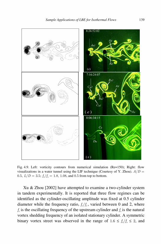
Sample Applications of LBE for Isothermal Flows 139
Xu & Zhou [2002] have attempted to examine a two-cylinder system
in tandem experimentally. It is reported that three flow regimes can be
identified as the cylinder-oscillating amplitude was fixed at 0.5 cylinder
diameter while the frequency ratio, fe/fs , varied between 0 and 2, where
fe is the oscillating frequency of the upstream cylinder and fs is the natural
vortex shedding frequency of an isolated stationary cylinder. A symmetric
binary vortex street was observed in the range of 1.6 ≤ fe/fs ≤ 2, and
Fig. 4.9. Left: vorticity contours from numerical simulation (Re=150); Right: flow
visualizations in a water tunnel using the LIF technique (Courtesy of Y. Zhou). A/D = 0.5, L/D = 3.5; fe/fs = 1.8, 1.08, and 0.5 from top to bottom.

140 Lattice Boltzmann Method and Its Applications in Engineering
alternative vortex shedding from both cylinders was seen in the cases of
0.8 ≤ fe/fs < 1.6 and 0 < fe/fs < 0.8, although the flow structure correspond-
ing to fe/fs = 0.8 ∼ 1.6 is totally different from that at fe/fs = 0 ∼ 0.8. Due
to the limitation of experiments, many aspects of the physics for this
flow remain to be clarified. For example, there was insufficient
information on how the oscillating amplitude of the upstream cylinder
and the spacing between the cylinders would affect the flow structure,
the information about the pressure field was not clear, too. Furthermore,
the dependence on the flow regimes of the drag and lift forces on the
cylinders was not easy to measure.
Guo and Zhou [2004] conducted a numerical investigation on this
flow using the D2Q9 LBGK model. The simulations are carried out in a
two-dimensional space at the same conditions as [Xu and Zhou, 2002].
Two circular cylinders with an identical diameter D are placed in a cross
flow in tandem, and the center-to-center spacing of them is set to be
3.5D. The upstream cylinder oscillates harmonically in the streamwise
direction at a fixed amplitude of A/D = 0.5. The Reynolds number based
on D and the free-stream velocity U is 150 ∼ 300 (the flow is essentially
tU/D
CD
520 530 540 550 560-4
-2
0
2
4
6
tU/D
CD
520 530 540 550 560
0
2
4
6
tU/D
CD
400 425 450 475
0
0.5
1
1.5
2
2.5
3
tU/D
CL
475 500 525 550
-0.2
-0.1
0
0.1
0.2
tU/D
CL
475 500 525 550
-2
0
2
tU/D
CL
400 425 450 475-3
-2.5
-2
-1.5
-1
-0.5
0
0.5
1
1.5
2
2.5
3
(a) (b) (c)
Fig. 4.10. Time histories of the drag and lift coefficients of the upstream and downstream
cylinders with A/D = 0.5, L/D = 3.5. (a) fe/fs = 1.8, (b) fe/fs = 1.08, (c) fe/fs = 0.5.
Dashed line: upstream cylinder; Solid line: downstream cylinder.

Sample Applications of LBE for Isothermal Flows 141
laminar) and fe/fs ranges between 0.5 and 1.8. The computational domain
is a 40D × 20D rectangular area.
Figure 4.9 compares the calculated flow structure with the
experimental data [Xu and Zhou, 2002]. The three flow regimes based on
the distinctive flow patterns identified by Xu & Zhou [2002] are
reproduced numerically. The excellent agreement in the flow structure
between the numerical and experimental data provides a validation for
the present numerical scheme. In all cases, vortex shedding from the
upstream cylinder is locked on with the cylinder oscillation.
At fe/fs = 1.8, vortices shed from the upstream cylinder are symme-
trically arranged; each structure embraces a pair of counter-rotating
vortices (binary vortices). The flow behind the downstream cylinder is
characterized by a binary street, consisting of two inner rows of
alternately arranged vortices and two outer rows of symmetrically
arranged binary vortices. The spatial arrangement of vortices about the
centerline results in a lift coefficient, CL , of no more than 0.2 on either
cylinder (Fig. 4.10a). The drag coefficient, CD
, on the downstream
cylinder is small but very large on the upstream cylinder (Fig. 4.10b).
Correspondingly, the time-averaged lift coefficient, LC , and root mean
square value, LC ′ , are small on both cylinders. On the other hand, the
time-averaged drag coefficient, DC , and root mean square value, DC ′ , are
both very large on the upstream cylinder. Although DC on the
downstream cylinder is 0.46, smaller than that (about 1) on an isolated
circular cylinder, the corresponding DC ′ reaches 0.48, one order of
magnitude larger than its counterpart of a single cylinder.
As fe/fs reduces to 1.08, alternative vortex shedding occurs from both
cylinders. The flow structure behind the downstream cylinder is
characterized by two rows of vortices: one consisting of single vortices,
and the other consisting of counter-rotating vortex pairs. The maximum
CL and CD (Fig. 4.10b) on the downstream cylinder increase significantly,
compared with fe/fs = 1.8. While the corresponding LC is small, and LC ′
increases greatly, exceeding that (0.45~0.75 for Re = 200 ∼ 700, Chen
1978) on a single cylinder, as a result from alternating vortex shedding
associated with both cylinders. Interestingly, DC as well as DC ′ climbs
considerably.

142 Lattice Boltzmann Method and Its Applications in Engineering
For fe/fs = 0.5, alternative vortex shedding occurs for both cylinders.
The successive vortices shed from the upstream cylinders will hit the
downstream cylinder alternatively, forming a single staggered street
downstream. While the maximum CD on the downstream cylinder is
smaller than that at fe/fs =1.08, the maximum CL increases marginally.
Accordingly, DC and DC ′ reduce appreciably, and LC ′ increases slightly.
Zdravkovich [1987] classified flows around two tandem stationary
cylinders into three flow regimes based on the behaviors of the free shear
layers separated from the upstream cylinder. The free shear layers do not
reattach on the downstream cylinder and roll up behind it to form the
vortex street for 1 < L/D < 1.2 ∼ 1.8, where the upper limit is dependent
on Re; they reattach on the upstream side of the downstream cylinder for
1.2 ∼ 1.8 < L/D < 3.4 ∼ 3.8. When L/D exceeds 3.4 ∼ 3.8, the shear
layers roll up alternately, forming vortices between the cylinders, both
cylinders generating vortices. Evidently, the flow structures at L/D =
3.5, shown in Fig. 4.9, fall into the third regime, that is, vortices are
generated between the cylinders and behind the downstream cylinder,
irrespective of the fe/fs value.
Simulations are also performed to investigate the effects of center-to-
center spacing. At L/D = 6.0, the shear layers separated from the
upstream cylinder are expected to have sufficient space to form vortices
before reaching the downstream cylinder. Therefore, given the same
A/D, the flow structures are likely to resemble those at L/D = 3.5. The
flow structures (Fig. 4.11) are indeed qualitatively the same as those in
Fig. 4.9 for the same fe/fs. Nevertheless, there is a slight increase in the
(a) (b) (c)
Fig. 4.11. Vorticity contours at L/D = 6 (A/D = 0.5, Re=150). (a) fe/fs = 1.8; (b) fe/fs = 1.08; (c) fe/fs = 0.5.
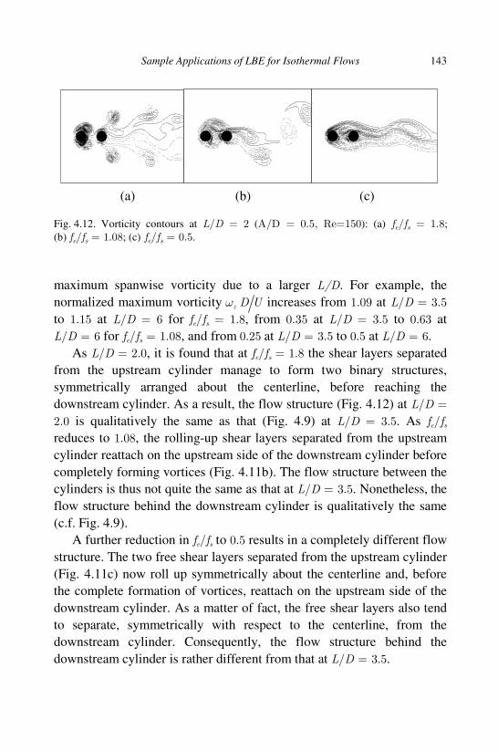
Sample Applications of LBE for Isothermal Flows 143
maximum spanwise vorticity due to a larger L/D. For example, the
normalized maximum vorticity z D Uω increases from 1.09 at L/D = 3.5
to 1.15 at L/D = 6 for fe/fs = 1.8, from 0.35 at L/D = 3.5 to 0.63 at
L/D = 6 for fe/fs = 1.08, and from 0.25 at L/D = 3.5 to 0.5 at L/D = 6.
As L/D = 2.0, it is found that at fe/fs = 1.8 the shear layers separated
from the upstream cylinder manage to form two binary structures,
symmetrically arranged about the centerline, before reaching the
downstream cylinder. As a result, the flow structure (Fig. 4.12) at L/D = 2.0 is qualitatively the same as that (Fig. 4.9) at L/D = 3.5. As fe/fs
reduces to 1.08, the rolling-up shear layers separated from the upstream
cylinder reattach on the upstream side of the downstream cylinder before
completely forming vortices (Fig. 4.11b). The flow structure between the
cylinders is thus not quite the same as that at L/D = 3.5. Nonetheless, the
flow structure behind the downstream cylinder is qualitatively the same
(c.f. Fig. 4.9).
A further reduction in fe/fs to 0.5 results in a completely different flow
structure. The two free shear layers separated from the upstream cylinder
(Fig. 4.11c) now roll up symmetrically about the centerline and, before
the complete formation of vortices, reattach on the upstream side of the
downstream cylinder. As a matter of fact, the free shear layers also tend
to separate, symmetrically with respect to the centerline, from the
downstream cylinder. Consequently, the flow structure behind the
downstream cylinder is rather different from that at L/D = 3.5.
(a) (b) (c)
Fig. 4.12. Vorticity contours at L/D = 2 (A/D = 0.5, Re=150): (a) fe/fs = 1.8; (b) fe/fs = 1.08; (c) fe/fs = 0.5.

144 Lattice Boltzmann Method and Its Applications in Engineering
4.5 Summary
The simplicity in programming has been recognized as an advantage of
LBE method in simulating fluid flows. In this chapter the algorithm
structure and basic subroutines of LBE are presented. Several examples,
including the lid-driven cavity flow, the flow around a fixed circular
cylinder, and the flow around an oscillating cylinder with a downstream
cylinder of identical diameter, are presented. The results of LBE are
compared with other numerical and/or experimental data reported in the
literature. These results demonstrate that LBE is a viable method for
incompressible fluid flow simulation.
It should be noted that the algorithm presented in this chapter is an
elementary implementation and is not optimized. Some methods to
improve the performance of LBE have been developed from different
viewpoints. For example, Pohl et al. [2003] employed a grid
compression technique to raise cache hit rate. Mattila et al. [2007]
introduced a swap algorithm to reduce memory consumption. Some
parallel algorithms were also developed for LBE on different computer
architectures [e.g., Desplat et al., 2001; Kandhai et al., 1998; Wellein
et al., 2005]. The most recent trend in this direction is the use of graphics
processing unit (GPU) architectures, which are ideally suited for LBE
[Bernaschi et al., 2009; Li et al., 2004; Tölke, 2009; Zhao, 2008].

145
Chapter 5
LBE for Low Speed Flows with
Heat Transfer
The LBE method has achieved great successes for isothermal or athermal
flows where temperature variations are ignored. In many scientific and
engineering problems, however, heat transfer is important or may be
dominant. Many efforts have been devoted to extend LBE to such flows.
In general, the existing LBE models for thermal flows can be classified
into three categories, i.e., multi-speed (MS) models, double-distribution-
function (DDF) models, and hybrid models.
In MS-LBE models, the fluid density, velocity, and temperature
are obtained from zeroth through second velocity moments of the
distribution function fi. Usually, in order to obtain the macroscopic
evolution equation of the temperature, a MS-LBE uses a larger set of
discrete velocities than that used in the corresponding isothermal model,
and the lattice can be decomposed into a set of basic sub-lattices (such as
square, hexagon, or cube), with identical link length in each sub-lattice.
In addition, the equilibrium distribution function (EDF) of the MS-LBE
model includes higher order velocity terms which are absent in that of an
isothermal model. A major shortage of the early MS-LBE models which
employ certain BGK collision operators is that the Prandtl number is
fixed. Some later models have overcome this problem, but the viscosity
appearing in the viscous dissipation in the energy equation may be
incorrect. Another shortcoming of the MS-LBE models is that the
numerical stability is not satisfied, which severely limits their applications.
In contrast, the DDF-LBE and hybrid models can effectively
overcome the aforementioned two limitations of the MS-LBE models. In
the DDF-LBE model, two types of distribution functions are used to

146 Lattice Boltzmann Method and Its Applications in Engineering
describe the evolutions of the velocity and temperature, respectively. The
LBE for the velocity is usually the same as the isothermal model, and
that for the temperature solves an advection-diffusion equation with the
same lattice or a simpler one. It has been demonstrated that the DDF-
LBE has a better numerical stability and can achieve a wider temperature
range than the MS-LBE. A major deficiency of DDF-LBE model is that
the equation of state is independent of temperature so that such models
are intrinsically only suitable for Boussinesq flows. Similar to DDF-LBE,
hybrid LBE models also treat the energy equation separately, and solve it
by some standard numerical schemes such as finite-difference method.
An advantage of this approach is that the pressure can be coupled with
the temperature explicitly.
As can be seen, all of the available thermal LBE models have their
own advantages and disadvantages, so that further developments and
refinements are still in need. In this chapter, we will present some basic
thermal LBE models.
5.1 Multi-speed Models
Earlier MS-LBE models usually adopt a lattice based on those of
isothermal models by including some new discrete velocities so that the
particles can move to farther neighboring grid points. In these models,
the discrete velocities are coupled with the associated lattices, and so
such models are also termed as space-filling models. According to the
terms of velocity expansion in the EDF, MS-LBE models can be
classified into low-order models and high-order ones. In the former type
the EDF contains some terms up to O(u3), while the latter type contains
terms up to O(u4), where u is the fluid velocity. It can be shown that the
corresponding macroscopic equations of the low-order models may
contain some undesirable artifacts, while those of the high-order MS-
LBE models have no such problem.
5.1.1 Low-order models
The first MS-LBE model was proposed by Alexander et al. [1993]. This
is a two-dimensional model (referred to as ACS model) containing 13

LBE for Low Speed Flows with Heat Transfer 147
discrete velocities associated with two hexagons with links of length c
and 2c, respectively:
0 (0, 0)=c , ( )cos , sini i i cσ σ θ θ=c , /3i i=θ π , 1 6i = ∼ , 1, 2σ = ,
(5.1)
where /x tc = δ δ is the lattice speed and we will assume c = 1 in the
following sections without statement otherwise. The BGK collision
operator is adopted in the ACS model, i.e.,
( )1( , ) ( , ) ( , ) ( , )eqi i t t i i if t f t f t f tσ σ σ σ σδ δ
τ + + − = − − x c x x x , (5.2)
where the equilibrium distribution function is defined by
( ) 2 2 3 2= + + ( ) + + ( ) + ( )eqi i i i if A B C D u E F uσ σ σ σ σ σ σ σ σ σ σ⋅ ⋅ ⋅ ⋅c u c u c u c u . (5.3)
Here the fluid velocity is still defined by i ii f= ∑u cσ σσρ , and the
coefficients Aσ ∼ Fσ are functions of the local density ii f= ∑ σσρ and
the internal energy 1 2
2| |i iie f= −∑ c uσ σσρ . These coefficients should be
chosen so that the following constraints are satisfied:
( )eqi
i
fσσ
ρ=∑ , ( )eqi i
i
fσ σ
σ
ρ=∑c u , ( )21| |
2
eqi i
i
f e− =∑ c uσ σ
σ
ρ ,
( )eqi i i
i
f eσ σ σ
σ
ρ ρ= +∑c c uu , ( )2| | ( ) 0eqi i i
i
f− − =∑ c u c uσ σ σ
σ
. (5.4)
One possible solution is [Alexander et al., 1993]:
( ) ( ) ( )2 2 20 1 2
42 5 4 , , 4 ,
2 9 36A e e A e e A e e
ρ ρ ρ− + = − = − +=
( ) ( )1 2
41 , 1 4 ,
9 36B e B e
ρ ρ= − = − +
( ) ( )1 2
42 3 , 1 6 ,
9 72C e C e
ρ ρ= − = − +
( ) ( ) ( )0 1 2
25 8 , 1 , 1 4 ,
4 9 72D e D e D e
ρ ρ ρ= − + = − + = −
1 2 1 2
4, , 0.
27 108E E F F
ρ ρ= − = = =

148 Lattice Boltzmann Method and Its Applications in Engineering
With the above parameters, it can be shown that the macroscopic
equations of the ACS model are
( ) 0t
ρρ
∂+ ∇ ⋅ =
∂u , (5.5)
( )
( ) pt
τ∂
+ ∇ ⋅ = −∇ + ∇ ⋅∂u
uuρ
ρ , (5.6)
( )
) :(e
e p qt
ρρ
∂+ ∇ ⋅ = − ∇ ⋅ + ∇ ⋅ + ∇
∂u u uτ , (5.7)
where p = ρe, and the viscous stress τ and the heat flux q are given by
2 ( )µ µ µ′= + ∇ ⋅S Iτ , Tκ= ∇q , (5.8)
in which the first and second dynamic viscosities and the thermal
conductivity are given by
1
2eµ ρ τ
= − , µ µ′ = − , 2κ µ= . (5.9)
It is easy to check that the specific heat capacities of the ACS model are
cp = (D + 2)R/2 and cv = DR/2, respectively, which means that the
Prandtl number is Pr = µcp/κ = 1. This limitation is due to the use of the
single relaxation BGK model for the collision, and other MS-LBGK
models also suffer from this problem.
Soon after the emergence of the ACS model, Qian [1993] developed
a series of MS-LBE models based on the DnQb-LBGK isothermal
models. The lattice employed in such a model is usually composed of a
group of sub-lattices Lσ , each of which having bσ links with length
cσσ = . For example, the lattice used in the D2Q13 model is composed
of 4 sub-lattices with σ = 0, 1, 2 and 4, respectively (Fig. 5.1). Generally,
the EDF of Qian’s MS-LBE models can be expressed as
2 2 2( ) 2
4
( )( ) ( )
2i
i seqi i
s
c uf A B D u
cσ σ σ σ σ σσ
ρ ω ⋅ − = + ⋅ + + ⋅
cc u uc
u, (5.10)
where ωσ is the same as that used in the isothermal DnQb-LBGK model.
The undetermined coefficients Aσ , Bσ , and Dσ satisfy the following

LBE for Low Speed Flows with Heat Transfer 149
conservation constraints,
1b Aσ σ
σ
=∑ , 21
2b A eσ σ
σ
σ =∑ , 2b B Dσ σ
σ
σ =∑ , 210
2b Dσ σ
σ
σ =∑ , (5.11)
where D is the spatial dimensions. The number of links of the sub-lattice
(or sub-discrete velocities in Lσ) bσ depends on the model and the spatial
dimension. For example, for the D2Q13 model shown in Fig. 5.1, b0 = 1
and b1 = b2 = b4 = 4. Furthermore, the following additional constraints
must be satisfied in order to obtain correct transport coefficients,
4 22( 2)b A D seσ σ
σ
σ = +∑ , 4 ( 2)b B D D seσ σ
σ
σ = +∑ , (5.12)
where s is an adjustable parameter. Based on these arguments, Qian
proposed a set of DnQb MS-LBGK models, which are listed as follows.
(1) D1Q5 model
The discrete velocities are given by c = [0,±1,±2], and the parameters in
Fig. 5.1. D2Q13 lattice form structure.

150 Lattice Boltzmann Method and Its Applications in Engineering
the EDF are
20 1 4
22 2
0 1 4
1 4 1 4
1 1 1, , , 1,
2 6 125 4
1 3 , 2 , ,2 3 12 2
2 1 1 1, , , .
3 2 24 24 6 24
sc
e e e eA e A e A
se seB B D D
ω ω ω= = = =
= − + = − = − +
= − = − + = − =
(2) D2Q13 model
The discrete velocities include those of the isothermal D2Q9 model and
4 additional velocities along the x and y directions with modulus 2 (i.e.
the sub-lattice with σ = 4 in Fig. 5.1),
4
2 2 0 0
0 0 2 2i
− = − c .
The parameters of the EDF are given by
20 1 2
4 1 1 1, , , ,
9 9 36 3scω ω ω= = = =
2 2 2 2
0 1 2 4
5 9 2 5 71 , , , ,
2 4 3 6 8 24 48
e e e e e e eA A A A= − + = − = = − +
1 2 4
2 1, , ,
3 4 24 8
se seB se B B= − = = − +
1 2 4
1 1 1, , .
18 12 18D D D= − = − =
(3) D3Q21 model
The discrete velocities include those of the D3Q15 model and 6
additional velocities along the x, y, and z axes with modulus 2,
4
2 2 0 0 0 0
0 0 2 2 0 0
0 0 0 0 2 2
i
− = − −
c ,
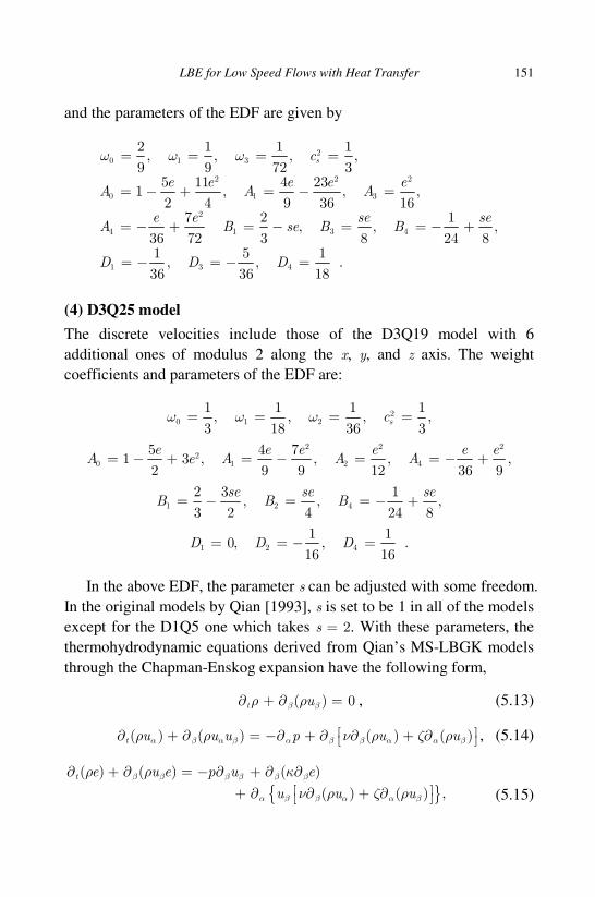
LBE for Low Speed Flows with Heat Transfer 151
and the parameters of the EDF are given by
20 1 3
2 2 2
0 1 3
2
4 1 3 4
1 3 4
2 1 1 1, , , ,
9 9 72 35 11 4 23
1 , , ,2 4 9 36 16
7 2 1, , ,
36 72 3 8 24 81 5 1
, , .36 36 18
sc
e e e e eA A A
e e se seA B se B B
D D D
ω ω ω= = = =
= − + = − =
= − + = − = = − +
= − = − =
(4) D3Q25 model
The discrete velocities include those of the D3Q19 model with 6
additional ones of modulus 2 along the x, y, and z axis. The weight
coefficients and parameters of the EDF are:
20 1 2
1 1 1 1, , , ,
3 18 36 3scω ω ω= = = =
2 2 2
20 1 2 4
5 4 71 3 , , , ,
2 9 9 12 36 9
e e e e e eA e A A A= − + = − = = − +
1 2 4
2 3 1, , ,
3 2 4 24 8
se se seB B B= − = = − +
1 2 4
1 10, , .
16 16D D D= = − =
In the above EDF, the parameter s can be adjusted with some freedom.
In the original models by Qian [1993], s is set to be 1 in all of the models
except for the D1Q5 one which takes s = 2. With these parameters, the
thermohydrodynamic equations derived from Qian’s MS-LBGK models
through the Chapman-Enskog expansion have the following form,
( ) 0t uβ βρ ρ∂ + ∂ = , (5.13)
( ) ( ) ( ) ( )t u u u p u uα β α β α β β α α βρ ρ ν ρ ζ ρ ∂ + ∂ = −∂ + ∂ ∂ + ∂ , (5.14)
( ) ( ) ( )
( ) ( ) ,
t e u e p u e
u u u
β β β β β β
α β β α α β
ρ ρ κ
ν ρ ζ ρ
∂ + ∂ = − ∂ + ∂ ∂ + ∂ ∂ + ∂
(5.15)

152 Lattice Boltzmann Method and Its Applications in Engineering
where 2(2/ ) sp D e c= =ρ ρ is the pressure, and the transport coefficients
are given by
2
1 2 1 2 1, 2 , .
2 2 2
D Dse s e e
D Dν τ ζ τ κ τ ρ
+ + = − = − − = −
(5.16)
5.1.2 High-order models
In the low-order MS LBE models given above, the EDFs only involve
terms up to O(u3). Chen et al. [1994] found that, however, the EDF
should contain terms of in order to obtain the correct momentum flux and
heat flux for deriving macroscopic equations, i.e.,
( ) 2 2 2
3 2 2 4
( ) ( ) ( )
( ) ( ,)i
eqi i i
i i
f A B C u D E u
F G u H u
σ σ σ σ σ σ σ σσ
σ σ σ σ σ
= + ⋅ + + ⋅ + ⋅
⋅ + ⋅ ++
c u c u c u
c u c u
(5.17)
where the undetermined coefficients Aσ ∼Hσ are quadratic polynomials of
the internal energy that can be expressed as,
20 1 2( )X x x e x eσ σ σ σρ= + + . (5.18)
Furthermore, the following constraints are required [Chen et al., 1994],
( ) ( ) ( ), , ,eq eq eqi i i i i i
i i i
f f f pσ σ σ σ σ σ
σ σ σ
ρ ρ ρ= = = +∑ ∑ ∑c u c c uu Ι (5.19)
( ) [ ],eqi i i i
i
f p δ= +∑c c c uuu uσ σ σ σ
σ
ρ (5.20)
( )2 2 22( 2)
( 4) ,eqi i i i
i
Dc f u p D pu pe
D
+= + + + +∑c c uu uu Iσ σ σ σ
σ
ρ (5.21)
where p = (2/D)ρe and [uδ]αβγ =uαδβγ +uβδαγ +uγδβα . In order to meet the
above conditions, Chen et al. pointed out that the discrete velocity set
should have enough symmetry. More specifically, the velocity tensors
,
n
ni i i
i
Tσ σ σ σ≡ ∑c c c
, n = 0, 1, ......, 6, (5.22)
must be all isotropic (note that the low order models can only give the
0∼4-th order isotropic tensors). To achieve this purpose, Chen et al.
chose a composite lattice based on a D-dimensional unit cube to define

LBE for Low Speed Flows with Heat Transfer 153
the discrete velocity set,
Perm ( 1, 1, , 1, 0, , 0, 0)
D p
i pki
p
kσ
−
= ∈ ± ±′ ±c c
, (5.23)
where the operator “Prem(⋅)” represents a set composed of all the
possible permutations of (⋅), k is a scaling coefficient of the basic lattice,
and it is clear that 2 2ic k pσσ = = . For example, for the D2Q13 lattice
shown in Fig. 5.1, the velocities of the sub-lattices (from top to bottom)
are 0 0′=c c , 1 11i i′=c c , 2 21i i
′=c c , and 4 12i i′=c c , respectively.
Based on such lattices and EDF, Chen et al. [1994] developed a series
of 1~3 dimensional DnQb MS-LBGK models, which are listed below.
(1) D1Q5 model
Discrete velocities: c = [0, ±1, ±2].
Parameters in the EDF:
22 2
0 1 4
5 41 3 , 2 , ,
2 3 12 2
e e e eA e A e A= − + = − = − +
1 4
2 1, ,
3 24 4
eB e B= − = − +
0 1 4
5 1 13 , , ,
4 3 2 48 8
e eC e C C= − + = − + = −
1 4 1 4
5 1 5 17 11 , , , ,
2 64 32 12 24
e eD D E E= − = − + = − =
1 1 4 0 1 4
5 1 1 1 1 1, , , , ,
4 4 64 4 12 48F G G H H H= = − = = = = − .
(2) D2Q16 model
Discrete velocities:
1 11 Prem( 1,0)i i= ∈ ±′c c , 2 21 Prem( 1, 1)i i= ∈ ± ±′c c ,
4 12 Prem2( 1,0)i i= ∈ ±′c c , 8 22 Prem2( 1, 1)i i= ∈ ± ±′c c .
Parameters in the EDF:
1 2 4 8
2 5 1 7 1 1, , , ,
3 6 6 24 24 12 96
e e e eC C C C
−= − + = − = − = −

154 Lattice Boltzmann Method and Its Applications in Engineering
1 2 4 8
2 1 1 1, , , ,
3 6 8 96 16 384 128
e e eD e D D D= − = − = − + = − +
1 2 4 8
1 2 4 8
1 2 4 8
1 2 4 8
1 1, , 0,
2 81 1 1, , , 0,
3 8 961 1 1 1, , , ,
6 48 96 7681 1 1, , , 0.
8 32 64
E E E E
F F F F
G G G G
H H H H
= − = − = =
= = = =
= − = − = − = −
= = − = − =
(3) D3Q40 model
Discrete velocities:
1 11 2 21Prem( 1,0, 0), Prem( 1, 1, 0)i i i i= ∈ ± = ∈ ±′ ±′c c c c ,
3 31 4 12Prem( 1, 1, 1), Prem2( 1, 0, 0)i i i i= ∈ ± ± ± = ∈ ±′ ′c c c c ,
12 32 Prem2( 1, 1, 1).i i= ∈ ± ± ±′c c
Parameters in the EDF:
2 2
1 2 3
2 2
4 12
1 2 3 4 8
1 2 3 4 12
1 2 3
4 29 8 5 1 15 19, , ,
15 36 135 8 15 16 2701 13 1 17
, ,60 36 540 240 2160
2 1, , 0, , 0,
3 6 24 121 7 53 23 1 2
, , , , 0,3 32 192 128 48
2 1, , ,
3 4 24 12 32
e e e e eA A A
e e eA A
e eB e B B B B
e e e eC C C C C
e e eD D D D
= − + = = − − −
= − − + = +
= − = = = − + =
−= − − = = − = =
= − = = − 4
12
1 2 3 4 12
1 2 3 4 12
1 2 3 4 12
1,
961
,768 1536
1 1 3, , 0, , 0,
2 8 641 1 1 1
, , , , 0,24 48 192 384
3 1 3 3 1, , , , ,
56 112 448 448 7168
e
eD
E E E E E
F F F F F
G G G G G
−= −
= − +
= = − = = − =
= = = = =
= − = = − = = −

LBE for Low Speed Flows with Heat Transfer 155
1 2 3 4 12
177 401 513 1, , , , 0.
2240 4480 8960 80H H H H H= − = = − = − =
Chen et al. [1994] have shown that with the above discrete velocity
sets and EDFs, the MS-LBGK models could give the standard
compressible Navier-Stokes equations with the following transport
coefficients
2 1
2e
Dµ τ ρ
= − ,
2
Dµ µ′ = − ,
2 1
2
De
Dκ τ ρ
+ = − . (5.24)
It is apparent that these high-order MS-LBGK models give a zero bulk
viscosity and a unit Prandtl number.
Chen et al. [1995] have simulated the thermal Couette flow with both
the high-order MS-LBGK models and Qian’s low-order models. It is
shown that the difference between the results of the two types of models
is significant for high Mach number flows, and usually the high-order
models could give better predictions. This fact indicates that the terms of
O(u4) in the EDF are critical for high speed flows.
5.2 MS-LBE Models Based on Boltzmann Equation
The MS-LBE models described above are designed in a top-down
fashion, i.e. the discrete velocities and the EDFs are determined by
enforcing the corresponding macroscopic equations to match the
thermohydrodynamic equations with certain accuracy. The parameters
determined in this way are somewhat empirical, and it is not an easy task
to find these parameters by solving the constraint equations. On the other
hand, it is known that the isothermal LBGK models can be obtained from
the continuous Boltzmann equation following certain systematic
discretization techniques. Similar approach can also be used to establish
MS-LBE models [Philippi et al., 2006; Shan et al., 2006].
5.2.1 Hermite expansion of distribution function
From kinetic theory, it is known that the distribution function f for
a Maxwell gas can be expanded into a series of Hermite tensor

156 Lattice Boltzmann Method and Its Applications in Engineering
polynomials, which is defined by
ζi
1
2 2( ) ( )
( 1)( ) ( 1) exp exp ( ),
2 2 ( )n
nn n n
i i
Hζ ζ
ζ ω ζζ ζ ω
−∂ ∂ = − − = ∇ ∂ ∂ (5.25)
where i = i1i2in and /2 2( )=(2 ) exp( /2)D− −ω ζ π ζ . The first few generalized
Hermite polynomials can be easily computed from Eq. (5.25), e.g.,
(0) 1H = , (1)i iH ζ= , (2)
ij i j ijH ζ ζ δ= − , (3) [ ]i j k ijkijkH ζ ζ ζ= − ζδ , (5.26)
where [ ]ijk i jk j ik k ijζ δ ζ δ ζ δ≡ + +ζδ . The tensor Hermite polynomials are
orthonormal with respect to the weight ω(ζ), i.e.,
i j ij( ) ( ) ( )( ) ( ) ( )m n n
mnH H dω δ δ=∫ ζ ζ ζ ζ , (5.27)
where ( )nijδ is zero unless i = (i1 i2 im) is a permutation of j = (j1 j2jn).
The Maxwellian distribution function ( )( , , )eqf tξx can be expanded in
terms of Hermite polynomials as [Harris, 1971],
i iax x( ) ( )( )
0
1( , , ) ( , ) ( , ) ( )
!
n neq M
n
f t f t Hn
∞
=
= ∑ξ ϑ η η , (5.28)
where the expansion coefficients are functions of time and space,
i ia( ) ( )1 ( )( ) ( )n neqf H dρ−= ∫ ξ η ξ . (5.29)
In Eq. (5.28), Mf is the local Maxwellian distribution function in the
form of
2
/2( , ) exp
(2 ) 2M
Df
ρ ηϑ
πϑ
= − η , (5.30)
where the parameters ϑ and η can have different choices. Three types of
ϑ and η were suggested by Philippi et al. [2006],
A: RTϑ θ= = and u( )/ θ=η ξ− .
B: ϑ θ= and / θ=η ξ .
C: 0ϑ θ= and 0/η ξ= θ , where 0 0RTθ = and T0 is a reference
temperature.
In order to determine the discrete velocities and the discrete EDF
for constructing thermal LBE, first the above expansion needs to be

LBE for Low Speed Flows with Heat Transfer 157
truncated at certain orders, i.e.,
i ix x xa( ) ( ) ( )( )
0
1( , , ) ( , , ) ( , ) ( , ) ( )
!
N
eq n neq MN
i
f t f t f t Hn
ϑ=
≈ ≡ ∑ξ ξ η η , (5.31)
where N is an integer. Then a numerical quadrature is chosen so that the
velocity moments of the truncated expansion hold up to a certain order,
x x c( ) ( )
1
( , , ) ( , , )b
eq eqk ki i iN N
i
f t d W f t=
=∑∫ ξ ξ ξ ξ , k = 0, 1, …, K (5.32)
where K is an integer, Wi and ci are the weights and abscissas of the
quadrature, respectively. The discrete velocities are then chosen to be the
abscissas ci . Therefore, the choice of quadrature plays a critical role in
determining the discrete velocities and the corresponding LBE model.
Equation (5.28) indicates that ( )eqNf can be expressed as
( )( ) ( , ) ( )eq MNNf f hϑ=ξ η η , (5.33)
where Nh is a polynomial of degree N. Therefore a natural choice of the
numerical quadrature in Eq. (5.32) is the Gauss-Hermite formulation of
degree N + K with the weight function ω(η), i.e.,
1
( ) ( ) ( )b
i i
i
d wω φ φ=
=∑∫ η η η η , (5.34)
where φ is a polynomial of degree N + K, wi and ηi are the weights
and integration nodes, respectively. From Eqs. (5.32) and (5.34) we can
identify that / ( , )Mi i iW w fρ ϑ= η , and ci can be obtained from ηi . The
discrete EDF is obtained by setting ( ) ( )( , , )eq eqi i iNf W f t= cx .
The continuous distribution function f(x, ξ, t) can also be expanded in
the tensor Hermite polynomials [Shan et al., 2006], from which we can
define the discrete distribution functions fi = Wi f(x, ci, t). The evolution
equation of fi , which is usually called as discrete velocity Boltzmann
equation (DVBE), can be deduced from the Boltzmann equation,
( )1· eqii i i i
c
ft
ff f
τ +
∂∇ = − − ∂ c . (5.35)
Further discretizations in time and space will lead to MS-LBE models.

158 Lattice Boltzmann Method and Its Applications in Engineering
The order of the truncated expansion of ( )eqf , N, and the highest
order of the velocity moments required in Eq. (5.32), K, determine the
consistency between the DVBE (and the resultant LBE) and the
continuous Boltzmann equation. In what follows we will discuss the
resultant DVBE models corresponding to the three different choices of fM
given by Eq. (5.30).
5.2.2 Temperature/flow-dependent discrete velocities
In the first choice, the local Maxwellian distribution function uses ϑ θ=
and u( )/ θ= −η ξ , which means that ( )( ) ( , )eq Mf f θ=ξ η . Therefore the
coefficients of its Hermite expansion are a0 = 1 and ( ) 0ni =a (n > 0), i.e.,
hN = 1. Consequently, for a given K one can just choose the Gaussian
quadrature of degree K, and the discrete EDF is simply as
( ) ( , )eq Mi i i if W f wθ ρ= =η . (5.36)
It is obvious that ( )eqif is independent of the fluid velocity. However, in
this case the discrete velocities are functions of both the fluid velocity
and temperature,
c ui i θ= + η . (5.37)
This means that the particle velocity changes locally with the
temperature and fluid velocity, which may bring many difficulties in
practical applications. Sun [1998] has proposed one LBE model based on
this idea, but the implementation is rather difficult.
5.2.3 Temperature-dependent discrete velocities
The second kind of Hermite expansion sets ϑ θ= and / θη = ξ in the
local Maxwellian distribution function, and so ( )( , , )= ( , )ˆeq Mf t fξ η −x uθ
with ˆ /=u u θ . The expansion coefficients are then
i i ia uu( ) ( ) ( )1ˆ( , ) ( ) ( ) ( )ˆn n nMf H d H dθ ω
ρ= − = +∫ ∫η η η η η η , (5.38)

LBE for Low Speed Flows with Heat Transfer 159
and the first few coefficients can be expressed as
(0) 1a = , (1) ˆi ia u= , (2) ˆ ˆij i jua u= , (3) ˆ ˆ ˆi j kijk ua u u= , (4) ˆˆ ˆ ˆk lkl iij juu ua u= . (5.39)
On the other hand, in order to make Eq. (5.34) hold exactly, we should
choose a Gaussian quadrature of degree Ν + Κ at least. Then the discrete
velocities are set to be ci iθ= η , and so the discrete equilibrium
distribution function can be expressed as
x c
uu c c Ic u
( ) ( )
2
ˆˆ ˆ( , , ) 1 ( )
: ( )1 .
2
eq eqi i i i i i i j i j ijN
i iii
uuf W f t w u
w
ρ η η η δ
θρ
θ θ
= = + + − + −⋅ = + + +
(5.40)
It should be noted that although the quadrature nodes ηi are some
constants, the discrete velocities ic can change in both time and space
through the local temperature. Consequently, the particles may not arrive
at lattice nodes during the propagation, which means that interpolations
or other techniques should be adopted in the computation [Pavlo et al.,
2002]. However, this numerical difficulty is not the main problem of
such DVBE (and LBE) models. A more serious problem is the coupling
between ci and x and t, which should be independent as that in the
continuous Boltzmann equation. As a result, in the DVBE (5.35) ic is
non-commutative with the temporal and spatial derivatives, i.e.,
( )k ki t i t i if f∂ ≠ ∂c c , ( )k k
i i i if f∂ ≠ ∂c c . (5.41)
Consequently, even though the discrete velocity moments can match the
continuous ones up to the required order, the macroscopic hydrodynamic
equations from the DVBE (5.35) may still be incorrect. For example,
although the discrete velocities can ensure that ( )eqii ii if f= =∑ ∑c c uρ ,
the continuity equation on the 0t time scale in the Chapman-Enskog
expansion is
0 0 0t
∂ + ∇ = ⋅ uρ
ρ θθ
, (5.42)
or
0 0 0
1( ) ln 0
2t ρ ρ ρ θ∂ + ∇ ⋅ = ⋅ ∇ ≠u u , (5.43)

160 Lattice Boltzmann Method and Its Applications in Engineering
which indicates that the DVBE (5.35) is inconsistent with the continuous
Boltzmann equation even at the Euler level.
5.2.4 Constant discrete velocities
The third Hermite expansion method uses 0ϑ θ= and 0/ θ=η ξ in
the Maxwellian distribution function Mf . In this case, ϑ and η are
independent of time and space, and Mf is a global equilibrium
distribution function. The equilibrium distribution function can then be
expressed as
2
0( ) /2
/2
ˆ( )( , , ) exp
ˆ(2 ) 2eq D
D
uf t
ηρ θρθ ω
πθ θ θ
− − − = − =
ux
ηξ , (5.44)
where 0ˆ /=θ θ θ . The expansion coefficients of f (eq) are
i i i
uua( ) ( ) ( )/2ˆ ˆ( ) (
ˆˆ(
ˆ) )n n nD H d H dθ ω ω θ
θ
− − = = + ∫ ∫η
η ξ η η η , (5.45)
and the first four coefficients can be evaluated as
(0) 1a = , (5.46)
(1) ˆˆ ˆ( )i i i iua d uω θη = + = ∫ η η , (5.47)
(2) ˆ ˆˆ ˆ ˆˆ( ) ( )( ) ( 1)ˆij i i j j ij i j ijuua d uuθθω η η δ θ δ = + + − = + − ∫ η η , (5.48)
u(3) ˆˆ ˆˆ ( 1)[ ]i j k ijkijk uua u θ= + − δ , (5.49)
uu(4) 2ˆ ˆˆ ˆˆ ( 1)[ ] ( 1) [ ]ˆi j k l ijkl ijklijkl uua uu θ θ= + − + −δ δδ , (5.50)
where
[ ]ijkl ij jk ik jl il jkδ δ δ δ δ δ= + +δδ ,
[ ]ijkl i j jk i k jl i l jk j k il j l ik k l iju u u u u u u u u u u uδ δ δ δ δ δ δ= + + + + +uu . (5.51)
In this kind of expansion, the discrete velocities obtained from the
quadrature (5.34) are independent of time and space. Actually, the
discrete velocities c 0i iθ= η are some constant vectors depending on
the selected quadrature. The discrete EDF corresponding to the above
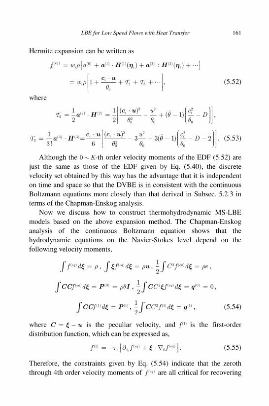
LBE for Low Speed Flows with Heat Transfer 161
Hermite expansion can be written as
a H a H
c u
( ) (0) (1) (1) (2) (2)
2 3
0
( ) : ( )
1 ,
eqi i i i
ii
f w a
w
ρ
ρθ
= + ⋅ + + ⋅ = + + + +
η η
T T
(5.52)
where
2 2 2
(2) (2)2 2
0 0 0
( )1 1 ˆ( 1)2 2
i iu cDθ
θ θ θ
⋅ = ⋅ = − + − −
cH
uaT ,
2 2 2(3) (3)
3 20 0 0
( )1 ˆ= 3 3( 1) 23! 6
ii iu cD
⋅⋅ = ⋅ − + − − −
c uca H
uθ
θ θ θT . (5.53)
Although the 0 ∼ K-th order velocity moments of the EDF (5.52) are
just the same as those of the EDF given by Eq. (5.40), the discrete
velocity set obtained by this way has the advantage that it is independent
on time and space so that the DVBE is in consistent with the continuous
Boltzmann equations more closely than that derived in Subsec. 5.2.3 in
terms of the Chapman-Enskog analysis.
Now we discuss how to construct thermohydrodynamic MS-LBE
models based on the above expansion method. The Chapman-Enskog
analysis of the continuous Boltzmann equation shows that the
hydrodynamic equations on the Navier-Stokes level depend on the
following velocity moments,
( )eqf d ρ=∫ ξ , u( )eqf d ρ=∫ ξ ξ , 2 ( )1
2eqC f d eρ=∫ ξ ,
( ) (0)eqf d ρθ= =∫C P IC ξ , 2 ( ) (0)10
2eqC f d = =∫C qξ ξ ,
(1) (1)f d =∫CC Pξ , 2 (1) (1)1
2C f d =∫C qξ , (5.54)
where C u= −ξ is the peculiar velocity, and (1)f is the first-order
distribution function, which can be expressed as,
0
(1) ( ) ( )0
eq eqc tf f fτ = − ∂ + ⋅ ∇ ξ . (5.55)
Therefore, the constraints given by Eq. (5.54) indicate that the zeroth
through 4th order velocity moments of ( )eqf are all critical for recovering
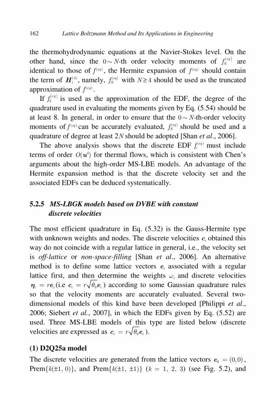
162 Lattice Boltzmann Method and Its Applications in Engineering
the thermohydrodynamic equations at the Navier-Stokes level. On the
other hand, since the 0 ∼ N-th order velocity moments of ( )eqNf are
identical to those of ( )eqf , the Hermite expansion of ( )eqf should contain
the term of (4)iH , namely, ( )eq
Nf with N ≥ 4 should be used as the truncated
approximation of ( )eqf .
If ( )4
eqf is used as the approximation of the EDF, the degree of the
quadrature used in evaluating the moments given by Eq. (5.54) should be
at least 8. In general, in order to ensure that the 0 ∼ N-th-order velocity
moments of ( )eqf can be accurately evaluated, ( )eqNf should be used and a
quadrature of degree at least 2N should be adopted [Shan et al., 2006].
The above analysis shows that the discrete EDF ( )eqif must include
terms of order O(u4) for thermal flows, which is consistent with Chen’s
arguments about the high-order MS-LBE models. An advantage of the
Hermite expansion method is that the discrete velocity set and the
associated EDFs can be deduced systematically.
5.2.5 MS-LBGK models based on DVBE with constant
discrete velocities
The most efficient quadrature in Eq. (5.32) is the Gauss-Hermite type
with unknown weights and nodes. The discrete velocities ci obtained this
way do not coincide with a regular lattice in general, i.e., the velocity set
is off-lattice or non-space-filling [Shan et al., 2006]. An alternative
method is to define some lattice vectors ei associated with a regular
lattice first, and then determine the weights ωi and discrete velocities
i ir= eη (i.e 0i ir θ=c e ) according to some Gaussian quadrature rules
so that the velocity moments are accurately evaluated. Several two-
dimensional models of this kind have been developed [Philippi et al.,
2006; Siebert et al., 2007], in which the EDFs given by Eq. (5.52) are
used. Three MS-LBE models of this type are listed below (discrete
velocities are expressed as 0i ir θ=c e ).
(1) D2Q25a model
The discrete velocities are generated from the lattice vectors 0 (0, 0)=e ,
Premk(±1, 0), and Premk(±1, ±1) (k = 1, 2, 3) (see Fig. 5.2), and

LBE for Low Speed Flows with Heat Transfer 163
the parameter r = 0.834659, while the weights in the EDF are given
by
2
2
0.235184, | |=0,
0.101817, | |= 2,=
5.92134 10 , | |=2,
2.00409 10 , | |=2 2,
i
i
i
i
i
w−
−
× ×
e
e
e
e
and
3
3
3
6.79523 10 , | |=3,
= 1.14376 10 , | |=3 2,
2.19788 10 , | |=4.
i
i i
i
w
−
−
−
× × ×
e
e
e
(2) D2Q25b model
The discrete velocities are generated from the lattice vectors 0 (0, 0)=e ,
Premk(±1, 0) (k = 1, 2, 3, 4), and Premk(±1, ±1 ) (k = 1, 2)
(Fig. 5.2.), the parameter r = 1.075607, and the weights in the EDF are
given by
2
2
0.239059, | |=0,
0.063158, | |=1,=
8.75957 10 , | |= 2,
3.11800 10 , | |=2,
i
i
i
i
i
w−
−
× ×
e
e
e
e
and
3
3
5
6.19896 10 , | |=2 2,
= 2.02013 10 , | |=3,
8.38224 10 , | |=4.
i
i i
i
w
−
−
−
× × ×
e
e
e
(3) D2Q37
The discrete velocities are generated from the lattice vectors 0 (0, 0)=e ,
Premk(±1, 0) (k = 1, 2, 3), Premk(±1, ±1) (k = 1, 2), and Prem(±1,
±2) (Fig. 5.3.), the parameter r = 1.196980, and the weights in EDF are
Fig. 5.2. Lattice vector of D2Q25a(left) and D2Q25b(right).
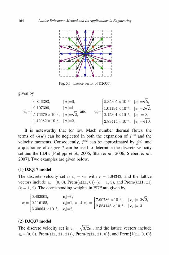
164 Lattice Boltzmann Method and Its Applications in Engineering
given by
2
2
0.846393, | |=0,
0.107306, | |=1,=
5.76679 10 , | |= 2,
1.42082 10 , | |=2,
i
i
i
i
i
w−
−
× ×
e
e
e
e
and
3
3
4
4
5.35305 10 , | |= 5,
1.01194 10 , | |=2 2,=
2.45301 10 , | | 3,
2.83414 10 , | |= 10.
i
i
i
i
i
w
−
−
−
−
× × × = ×
e
e
e
e
It is noteworthy that for low Mach number thermal flows, the
terms of O(u4) can be neglected in both the expansion of ( )eqf and the
velocity moments. Consequently, ( )eqf can be approximated by ( )3eqf , and
a quadrature of degree 7 can be used to determine the discrete velocity
set and the EDFs [Philippi et al., 2006; Shan et al., 2006; Siebert et al.,
2007]. Two examples are given below.
(1) D2Q17 model
The discrete velocity set is i ir=c e with r = 1.64343, and the lattice
vectors include e0 = (0, 0), Premk(±1, 0) (k = 1, 3), and Premk(±1, ±1)
(k = 1, 2). The corresponding weights in EDF are given by
2
0.402005, | |=0,
= 0.116155, | |=1,
3.30064 10 , | |=2,
i
i i
i
w−
×
e
e
e
and 5
4
7.90786 10 , | | 2 2,
2.584145 10 , | | 3.
i
i
i
w−
−
× == × =
e
e
(2) D3Q37 model
The discrete velocity set is 3/2i i=c e , and the lattice vectors include
e0 = (0, 0), Prem(±1, ±1, ±1), Prem2(±1, ±1, 0), and Premk(±1, 0, 0)
Fig. 5.3. Lattice vector of D2Q37.

LBE for Low Speed Flows with Heat Transfer 165
(k = 1, 2, 3). The weights in EDF are
1 / 12, | | 0,
1 / 12, | | 1,
1 / 27, | | 3,
i
i i
i
w
== = =
e
e
e
and
2 / 135, | |=2,
= 1 / 432, | |=2 2,
1 / 1620, | |=3.
i
i i
i
w
e
e
e
5.3 Off-Lattice LBE Models
Due to the coupling between the discrete velocities and the underlying
lattices, the MS-LBE models described so far usually involve a large
discrete velocity set in order to satisfy the necessary moment constraints.
On the other hand, off-lattice LBE models can release this problem by
decoupling the discrete velocity set and the lattice. But due to this
decoupling, the particles do not evolve on the lattice any more in such
LBE models, and some special treatments such as interpolation must be
employed.
The first off-lattice LBE may be attributed to Pavlo et al. [1998], who
developed a D2Q17 model based on a lattice consisting of two composite
octagons, where the discrete velocities are given by
0 (0, 0)=c , = = cos( /4), sin( /4)i pi p i iπ π′ c c , = 0 ~ 7i , = 1, 2p .
(5.56)
In order to make the computational mesh match these discrete velocities
as much as possible, Pavlo et al. employed the square lattice used in the
standard D2Q17 for spatial discretization (see Fig. 5.4). As such, in the
streaming step, only those particles with velocities 0c , 0p′c , 2p′c , ..., 6p′c
can reach the lattice nodes, while the others will fail. Pavlo et al. [1998]
suggested using a second-order interpolation scheme as a supplemen-
tation. It was shown that such interpolation method did not cause serious
numerical diffusion, and the stability analysis indicated that this model
has a better numerical stability than the aforementioned D2Q13 models
based on hexagon and square lattice as well as the standard D2Q17
model based on the composite square lattice. A three-dimensional
D3Q53 model was also constructed following a similar approach.

166 Lattice Boltzmann Method and Its Applications in Engineering
Watari and Tsutahara [2003] proposed a similar MS-LBE model (WT
model), which uses a composite lattice with four octagons. The discrete
velocities are given by )0 (0, 0=c , cos( /4), sin( /4)pi pc i iπ π = c , 0 7i = ∼ , 1 4p = ∼ , (5.57)
where the cp’s are undetermined parameters. The EDF of the WT model
is given as,
22 4 2 2( )
2 2
3 4
3 3
( )1 1 1
2 8 2 2 2
( ) ( ),
6 24
pi pieqpi p
pi pi
u u u uf
e e e e e e
e e
ω ρ ⋅ ⋅ = − + + − + −
⋅ + + ⋅
c u c u
c u c u (5.58)
where the weights ωp depend on the magnitude of the discrete velocities.
With the consideration of numerical stability, Watari and Tsutahara
[2003] suggested setting (c1, c2, c3, c4) = (1, 1.92, 2.99, 4.49), and the
corresponding ωi can be determined accordingly. To discretize the DVBE
(5.35) with these discrete velocities, an explicit scheme was suggested
[Watari and Tsutahara, 2003],
( )
y( , ) ( , )
( , ) ,
pi pi
pi pi pix piy
eqpi pi
c
f ff t t f t t c c
tf t f
x
τ
∂ ∂
∂ ∂
+ ∆ = −∆ + ∆ − −
x x
x
(5.59)
where the spatial derivatives were discretized by upwind schemes.
Fig. 5.4. Discrete velocities and computation mesh of the D2Q17 based on octagons.

LBE for Low Speed Flows with Heat Transfer 167
Recently Gan et al. [2008] developed another finite difference
scheme based on the WT model. Instead of solving DVBE (5.35) directly,
they suggested solving the following modified DVBE with an additional
dispersion term and an artificial viscosity term,
( ) 3 21pi eqpi pi pi pi pi pi pi pi
c
ff f f A f B f
tα α
τ
∂ + ⋅ ∇ = − − + ∂ + ∇ ∂c , (5.60)
where piA α and piB α are functions depending on the discrete velocity cpi.
Gan et al. [2008] used the Lax-Wendroff (LW) scheme to discretize the
left hand side of the equation and the central difference scheme is used to
the right hand side. Numerical results showed that this LW-LBE has
good numerical accuracy and stability.
Shan et al. [2006] also developed some off-lattice models based on
the Gauss-Hermite quadrature. A few examples for low Mach number
flows, in which ( )3eqf and the 7th-degree Gaussian quadrature are used,
are given below (discrete velocities are given by 0i iθ=c e and the ei’s
are the corresponding lattice vectors ).
(1) D1Q4 model
The lattice vectors are , and the corresponding weight
coefficients are given by (3 6) / 12iw = ± .
(2) D2Q12 model
The lattice vectors are defined by Prem(±r, 0), Prem(±s, ±s), and
Prem(±t, ±t), with 6r = , , and . The
weight coefficients are
1/36, | | ,
(5 2 5)/45, | | 2 ,
(5 2 5)/45, | | 2 .
i
i i
i
r
w s
t
== + = − =
e
e
e
(3) D2Q16 model
The lattice vectors consist of Prem(±r, 0), Prem(±s, 0), and Prem(±r,
±s), with and . The weight coefficients are
168 Lattice Boltzmann Method and Its Applications in Engineering
(5 2 6)/48, | | ,
(5 2 6)/48, | | ,
1/48, | | 6.
i
i i
i
r
w s
− == + = =
e
e
e
(4) D3Q27 model
Lattice vectors consists of e0=(0, 0), Prem(±r, 0, 0), Prem(±s, ±s, 0),
and Prem(±t, ±t, ±t), with , , and
. The weight coefficients are
(720 8 15)/2205, | | 0,
(270 46 15)/15435, | | ,
(162 41 15)/6174, | | 2 ,
(783 202 15)/24696, | | 3 .
i
i
i
i
i
rw
s
t
+ = − == + = − =
e
e
e
e
Based on the above discrete velocities and the corresponding EDFs,
one can solve the corresponding DVBE (5.35) using certain numerical
schemes, which will lead to non-standard MS-LBE models for thermo-
hydrodynamic problems.
5.4 MS-LBE Models with Adjustable Prandtl Number
The low-order, high-order, and kinetic-theory-based MS-LBE models
presented above all give a fixed Prandtl number, which severely limits
their applications. This difficulty can be resolved by introducing some
additional parameters. For example, Chen et al. [1997] developed a two-
relaxation-time model,
ı( , ) ( , )i i t t i if t f tδ δ+ + − = Ω + Ωx c x , (5.61)
where
( ) ( )ı ı ı
( ) ( )
1 2
1 1,eq eq
i i if f f fτ τ
Ω = − − Ω = − − , (5.62)
where ı i= −c c . It is easy to verify that the collision process satisfies
conservation laws due to the symmetry of the lattice.

LBE for Low Speed Flows with Heat Transfer 169
The Chapman-Enskog analysis shows that the recovered macroscopic
equations of LBE (5.61) are
( ) 0t
ρρ
∂+ ∇ ⋅ =
∂u , (5.63)
( )
( ) pt
ν
ρρ
∂+ ∇ ⋅ = −∇ + ∇ ⋅
∂u
uu τ , (5.64)
( )
( ) ( ) :e
e p Tt
κ
ρρ κ
∂+ ∇ ⋅ = ∇ ⋅ + ∇ ⋅ ∇ + ∇
∂u u uτ , (5.65)
where
2 ( )v vν µ λ= + ∇ ⋅ IS uτ , 2 ( )k kκ µ λ= + ∇ ⋅ IS uτ , (5.66)
and the transport coefficients are given by
2 1
2v ve
Dµ ρ τ
= − ,
2
4 1
2v ve
Dλ ρ τ
= − − , (5.67)
2 1
2k ke
Dµ ρ τ
= − ,
2
4 1
2k ke
Dλ ρ τ
= − − , (5.68)
2 1
2k
De
Dκ ρ τ
+ = − , (5.69)
where
1 2
1 1 1
vτ τ τ= + ,
1 2
1 1 1
kτ τ τ= − . (5.70)
Accordingly, the Prandtl number is
2 1
Pr2 1
v p v
k
cµ τ
κ τ
−= =
−, (5.71)
which means that the Prandtl number can be adjusted by changing the
values of the two relaxation times τ1 and τ2. However, it is noted that the
viscous stress in the dissipation term in the energy equation is τk , which
is inconsistent with that appeared in the momentum equation (i.e. τν).
Recently Prasianakis and Boulouchos [2007] proposed a similar two-
relaxation-time model, which starts from the following DVBE,
( )* *
1 2
1 1 eqii i i i i i
ff f f f f
t τ τ + ⋅ ∇ = − − − −
∂∂ c , (5.72)

170 Lattice Boltzmann Method and Its Applications in Engineering
where *if is an intermediate state. The physical meaning of this collision
model is that the non-equilibrium state first relaxes to the intermediate
state *if with a time scale τ1, and then to the local equilibrium state
( )eqif
with another time scale τ2. It is clear that the model reduces to the
standard BGK model as τ1 = τ2. In the above model, the intermediate
state plays a key role. In general it can be assumed that
( )* *eqi i if f fδ= + , (5.73)
where the correction *ifδ can be determined by projecting the DVBE onto
the moment space and then transforming back to the velocity space. For
example, the correction terms of D2Q9 model can be expressed as
* * * * * * * * *
* * * *
10, 2 , 2 ,2 ,2 , , ,
4, ,
i x y x y x y y x
x y x y
fδ δψ δψ δψ δψ δψ δψ δψ δψ
δψ δψ δψ δψ
= − − + −− − −
(5.74)
where
* ( ) ( )2 ( )eq equ P Pα α α γ αγ αγδψ ψ ψ= − − − , 2i i i
i
c c fα αψ = ∑ , i i i
i
P c c fα α β= ∑ ,
( )( ) 2 eqeqi i i
i
c c fα αψ =∑ , ( )( ) eqeqi i i
i
P c c fα α β=∑ . (5.75)
The corresponding macroscopic equations of the DVBE (5.72) can be
obtained by the Chapman-Enskog analysis, in which the viscosity
coefficients and thermal conductivity are
1 0µ τ ρθ= , 2 0
1
2κ τ ρθ= . (5.76)
Therefore the Prandtl number of this model is Pr = 4τ1/τ2, which can be
adjusted by changing τ1 and τ2. The LBE model can be obtained by
discretizing the DVBE (5.72) with certain numerical schemes. But
unfortunately the consistency of the viscous stress in the momentum and
energy equations was not discussed by Prasianakis and Boulouchos [2007].
Some more general two-relaxation-time LBE models were also
developed [Chen et al., 1997; Teixeira et al., 2000]. For instance, with
discrete velocities based on composite lattices, the collision operators can
be written as,
( ) ( )( ) ( )
21 2 1
1 1 1( )eq eq
pi pi pi pi pj pj pj
jp pi
Df f f f
b cτ τ τ
Ω = − − − − ⋅ − ∑ c c , (5.77)

LBE for Low Speed Flows with Heat Transfer 171
where bp is the number of links of the sub-lattice p. The hydrodynamic
equations recovered from this LBE are again those given by Eqs. (5.63)
~(5.65), with the following viscosity and thermal conductivity,
1
2 1
2v e
Dµ ρ τ
= − , 2
2 1
2
De
Dκ ρ τ
+ = − . (5.78)
Similar to the two-parameter model of Chen et al. [1997], the Prandtl
number of the above LBE can be adjusted by changing the values of τ1
and τ2, but the viscous stress in the momentum equation is still
incompatible with that in the energy equation. It is argued by some
researchers that for any collision operators such inconsistency will
appear, given that the moments corresponding to the viscous tensor and
the heat flux relax with different rates [McNamara et al., 1995; Shan
et al., 2006; Teixeira et al., 2000]. This also indicates the inherent
deficiency of MS-LBE models.
To overcome this disadvantage, McNamara et al. [1997] constructed
a MS-LBE model (referred to as MGA model) in which the collision
process is carried out in moment space. Clearly, this feature is similar to
that of the multi-relaxation-time model developed by d′Humères [1992].
But with a larger discrete velocity set, the MGA model is able to produce
the correct thermohydrodynamic equations. An example is a D3Q27
model which uses 27 discrete velocities, whose collision process can be
expressed as
( ))( , ) ( , ) eqi i ij j j
j
f t f t f f′ = + Ω −∑x x . (5.79)
This process is achieved by relaxing different velocity moments in the
moment space. Specifically, the five low-order velocity moments, ρ, j = ρu, and ρe, are conserved variables and do not change in the collision
processes. The high-order velocity moments associated with viscous
stress and heat flux are relaxed as follows,
( ) ( )1 12 2
3 3( ) ( 1) ( )ne nei i i i v i i i i
i i
c c c f c c c fα β αβ α β αβδ λ δ′− = + −∑ ∑ , (5.80)
( ) ( )2 2( 1)ne nei i i i i i
i i
C f C fκλ′ = +∑ ∑C C , (5.81)
where λν and λκ are the eigenvalues of the collision operator Ω. It can be
shown that the transport coefficients corresponding to this collision

172 Lattice Boltzmann Method and Its Applications in Engineering
operator are
2 1
3 2v teµ λ ρ δ
= − + ,
2 1
3 2k teκ λ ρ δ
= − + . (5.82)
Because the third-order velocity moments are relaxed in the frame
moving with the fluid rather than a fixed one, the viscous stress in the
momentum equation is now compatible with that in the energy equation.
However, practical simulations indicate that the MGA model suffers
from serious numerical instability [McNamara et al., 1997], and the
recent linear analysis also shows that the momentum and energy modes
in MS-LBE models have an unphysical coupling, which seriously affects
the numerical stability [Lallemand and Luo, 2000].
5.5 DDF-LBE Models without Viscous Dissipation and
Compression Work
The multi-speed LBE models are a straightforward extension of
isothermal models. As mentioned above, the MS-LBE models usually
involve a large discrete velocity set which requires high storage and
computational costs. Furthermore, the numerical stability of such models
is also not satisfactory.
In many problems, the compression work and viscous dissipation can
be neglected. In such cases, the temperature can be regarded as a scalar
which is governed by a convection-diffusion equation. Consequently, the
velocity and temperature fields can be solved separately, which means
that we can simulate the velocity field with an isothermal LBE and the
temperature field with another one for convection-diffusion equation.
This idea was first adopted in a model by Bartoloni et al. [1993], where
the temperature was treated as a pure passive scalar that has no effects on
the velocity field. Since then, a variety of LBE models with double
distribution functions (DDF-LBE) have been developed from different
ways.
5.5.1 DDF-LBE based on multi-component models
Based on a multi-component LBE model, Shan constructed a DDF-LBE
model which treats the temperature as a component of fluid mixture
LBE for Low Speed Flows with Heat Transfer 173
[Shan, 1997]. The effect of temperature on the velocity field is modeled
following an approach similar to that in LBE for binary mixtures.
Specifically, this model uses the following multi-component LBE
model:
,( )1( , ) ( , ) ( , ) ( , )eq
i i t t i i if t f t f t f tσσ σ σ
σ
δ δτ + + = − − x c x x x , (5.83)
for σ = 1, 2, …, S, where S is the number of components in the mixture,
ifσ is the distribution function of the component σ, and ,( )eq
ifσ is the
corresponding EDF,
( ) 2 ( ) 2( )
,( )
2 4 2
( ) ( )1
2 2
eq eqeqieq i
i i
s s s
uf
c c c
σ σσ σσω ρ
⋅ = + + −
⋅
c uc u, (5.84)
in which i if σσρ = ∑ and ( )/ii i
f σσ σρ= ∑u c are the density and velocity
components of σ, respectively, and ( )eqσu is the equilibrium velocity that
is not necessarily equal to uσ; In the absence of internal interactions and
external forces, it is assumed that the equilibrium velocities of all
components share a common one,
( )
1 1
S S
eq eq
j j
j j j
j j
σ
ρ ρ
τ τ= =
= ≡ ∑ ∑u
u u . (5.85)
On the other hand, if the component σ is subject to a body force Fσ , the
equilibrium velocity is given by
( ) ( ) teq eq σ σσ
σ
τ δ
ρ= +u
Fu . (5.86)
Shan suggested using the above LBE model for binary mixtures
(S = 2) to model thermal flows: the fluid motion is simulated by
component A, while the temperature is simulated by component B, under
the assumption that the two components share a common velocity. If
only the gravity is considered, A A tτ δ+u g will be used in the EDF, and
the density, velocity, and temperature of the fluid are defined as,
Ai
i
fρ = ∑ , 2
ti iA
i
fδ
ρ ρ= +∑u c g , i
i
BT f= ∑ . (5.87)

174 Lattice Boltzmann Method and Its Applications in Engineering
The corresponding macroscopic equations can be obtained via the
Chapman-Enskog expansion,
( )=0t
ρρ
∂+ ∇ ⋅
∂u , (5.88)
( )
( )( ) 2pt
ρρν ρρ+ =
∂∇ ⋅ ⋅− +
∂∇ + ∇uu
uS g , (5.89)
( )·T
T Tt
α+ ∇∂
= ∇ ⋅∂
∇u , (5.90)
where 2sp c ρ= , ν and α are the kinematic viscosity and thermal diffusivity,
respectively,
2 1
2tAscν τ δ
= − , 2 1
2tBscα τ δ
= − . (5.91)
Therefore, the corresponding Prandtl number of this model is Pr = ν/α =
(2τA − 1) / (2τB − 1), which can be adjusted by changing τA and τB.
5.5.2 DDF-LBE for non-ideal gases
Palmer and Rector [2000a, 2000b] proposed another DDF-LBE model
which can be used to simulate thermal flows of non-ideal gases. The
model adopts a velocity distribution function if and an internal energy
distribution function ig to simulate the velocity and temperature fields
respectively,
( )
1
1( , ) ( , ) ( , ) ( , )eqi i t t i i if t f t f t f tδ δ
τ + + = − − x c x x x , (5.92)
( )
2
1( , ) ( , ) ( , ) ( , )eqi i t t i i ig t g t g t g tδ δ
τ + + = − − x c x x x , (5.93)
where the two EDFs are defined by
2
0 2( )
2 2
2 4 2
, 0,2
( ), 0,
2 2
i
eq s
iii
s s s
i
ui
cf
ui
c c c
ω ρ χ
ω ρ χ
− = = + + − ≠
⋅
⋅ c uc u (5.94)
( ) ( )eq eqi ig ef= . (5.95)

LBE for Low Speed Flows with Heat Transfer 175
Here the parameters χ0 and χ are related by 0 0 1iiχ ω χ ω+ =∑ , or
0 0 0(1 )/χ χ χω ω= − + . The fluid density, velocity, and temperature are
defined as
i
i
fρ = ∑ , i i
i
fρ = ∑u c , i
i
T gρ =∑ . (5.96)
It is obvious that ( )ieqf is the EDF of the standard isothermal LBE as
χ = 1. The Chapman-Enskog analysis shows that the recovered
macroscopic equations of this LBE are just as those given by Eqs. (5.88)
to (5.90) (without the body force) with the same viscosity and thermal
diffusivity. As 1≠χ , however, some errors exist in the momentum
equations, which can be ignored if the time step is sufficiently small.
Meanwhile, the equation of state of the LBE is also related to χ , 2sp c ρχ= , which means that an equation of state for non-ideal gases can
be obtained by selecting an appropriate formulation ofχ .
5.5.3 DDF-LBE for incompressible flows
DDF-LBE models, which treat the velocity and temperature fields
separately, make use of an intrinsic assumption that the temperature
variations have little effects on the fluid motion. This assumption is valid
only for small Mach number flows, in which the fluid can be regarded as
incompressible and the fluid density can be considered to be constant
except in the buoyancy term (Boussinesq assumption). Under such
circumstances, the governing equations for the velocity and temperature are
=0∇ ⋅ u , (5.97)
20( )P T
tTν β+ ⋅ = −∇ + −
∂∇ +
∂∇u u g
uu , (5.98)
2TT T
tα+ ⋅ ∇ =
∂∇
∂u , (5.99)
where P = p/ρ0 is the reduced dynamic pressure, β is the thermal
expansion coefficient, and T0 is a referenced temperature.
In order to solve the above equations, Guo et al. [2002] constructed a
type of DDF-LBE models based on incompressible LBE models. For
example, the D2Q9 model of this type can be written as,
( )
1
1( , ) ( , ) ( , ) ( , ) ,eqi i t t i i i t if t f t f t f t Fδ δ δ
τ + + = − − + x c x x x (5.100)

176 Lattice Boltzmann Method and Its Applications in Engineering
for 0 8i = ∼ , and
( )
2
1( , ) ( , ) ( , ) ( , ) ,eqi i t t i i ig t g t g t g tδ δ
τ + + = − − x c x x x (5.101)
for 1 4i = ∼ . Here ( )eqif are given by Eq. (3.16), and the EDF for the
temperature distribution function is defined by
( )
21 2
4
eq ii
TT
c
= +
⋅
c u, 1 4i = ∼ . (5.102)
The velocity, pressure, and temperature, are defined as
8
1
i i
i
f=
= ∑u c , 82
0
1
( )4
i
i
cP f s
σ =
= + ∑ u ,
4
1
i
i
T g=
= ∑ , (5.103)
where σ is the parameter in ( )eqif (see Eq. (3.16) in Chap. 3).
In the original model, the forcing term Fi is suggested to take the
following form,
02( ), 2, 4,
20, other.
i
i
T T iF c
β ⋅ − ==
c g
(5.104)
It can be verified easily that 0iiF =∑ , 0( )i ii F T T= ≡ −∑ gc F β , and
0i i ii F =∑ c c . Therefore, the zeroth through second velocity moments of
Fi defined in this way are the same as those of 2/i i i sF c′ ⋅= Fcω . As
discussed in Chapter 3, the forcing term defined this way will produce
some artifacts. However, if the Mach number and temperature variations
are small, the error due to this forcing term is not significant. In such
cases it can be shown that Eqs. (5.97)-(5.99) can be recovered from the
above DDF-LBE, with the following transport coefficients,
2
1
1
3 2t
cν τ δ
= − ,
2
2
1
22t
cα τ δ
= − . (5.105)
The corresponding Prandtl number is therefore 21 23
Pr = ( 0.5)/( 0.5)− −τ τ .
The above incompressible DDF-LBE model can also be extended to
three-dimensional flows. A small advantage of such models is that the
LBE for the energy equations uses only 2D discrete velocities, which
LBE for Low Speed Flows with Heat Transfer 177
needs less computational memory than the aforementioned DDF-LBE
models. Furthermore, compressibility errors in such models can be
reduced, as their isothermal counterparts.
5.6 DDF-LBE with Viscous Dissipation and Compression
Work – Internal Energy Formulation
The DDF-LBE models presented in the above sections all neglect the
viscous dissipation and the compression work, which may be important
in some cases. The first DDF-LBE with the consideration of these two
factors is due to He et al. (HCD model) [1998], which introduces an
internal energy distribution function based on the continuous Boltzmann
equation.
5.6.1 Internal energy distribution function
The HCD model starts from the continuous Boltzmann equation,
( )f
ft
f+ ⋅ ∇ = Ω∂∂
ξ , (5.106)
where ( , , )f f tξ= x is the velocity distribution function. For monatomic
gases, the density ρ, velocity u, and internal energy e, are determined as
f dρ = ∫ ξ , f dρ = ∫u ξ ξ , 21( )
2 2
DRTe u f dρ ξ= = −∫ ξ . (5.107)
If we introduce an internal energy distribution function,
2( )
( , , )2
u fg t
ξ −=x ξ , (5.108)
the internal energy can then be defined as,
e gdρ = ∫ ξ . (5.109)
According to the Boltzmann equation (5.106), the evolution equation
for the international energy distribution function g can be deduced,
2( )
( ) ( )2t
ugg f fq g fq
ξ −+ ⋅ ∇ = ≡ Ω
∂−
∂Ω −ξ , (5.110)

178 Lattice Boltzmann Method and Its Applications in Engineering
where
( )t
q = − ⋅ + ⋅ ∇
∂∂u
u uξ ξ . (5.111)
He et al. suggested using the BGK models with different relaxation
times to approximate the collision operators Ω(f) and Ω(g),
( )( )1eq
u
ff f
tf
τ+ ⋅ ∇ = − −
∂∂
ξ , (5.112)
( )( )1eq
e
ft
gg g g q
τ+ ⋅ ∇ = −
∂∂
− −ξ , (5.113)
where ( )eqf is the Maxwell distribution, and g(eq) is defined by
2 2 2
( ) ( )
/2
( ) ( ) ( )exp
2 2(2 ) 2eq eq
D
u u ug f
RT RT
ξ ρ ξ ξ
π
− − − = = − . (5.114)
Using the Chapman-Enskog expansion we can obtain the following
thermohydrodynamic equations from Eqs. (5.112) and (5.113),
( ) 0t
ρρ
∂+ ∇ ⋅ =
∂u , (5.115)
( )
( )t
pρ
ρ+ = −∇∂
+∇ ⋅ ∇ ⋅∂u
uu τ , (5.116)
( )
( ) ( ) : pt
ee e
ρρ ρα
∂∇ ⋅ ∇ ⋅+ = ∇ + ∇ ∇ ⋅
∂−u u uτ , (5.117)
where p = ρRT is the pressure, 2ρν= Sτ is the viscous stress with
uRTν τ= , and ( 2) /eD RT D= +α τ is the thermal diffusivity. These
equations are similar to those corresponding to the continuous
Boltzmann-BGK equation, but the Prandtl number now can be tuned
to be consistent with that of the Boltzmann equation by adjusting eτ .
Furthermore, the viscous dissipation in the energy equation is also
consistent with that in the momentum equation.
In the above discussions no body forces are considered. In the
presence of a body force F, a forcing term F should be included in

LBE for Low Speed Flows with Heat Transfer 179
Eq. (5.112),
( )( )1eq
u
ff f f
tF
τ+ ⋅ ∇ =
∂∂
− − +c , (5.118)
where
( )( )
eqF f fRT
⋅ −= ⋅ ∇ ≈
uFF ξ
ξ. (5.119)
5.6.2 Lattice Boltzmann equations
The HCD model is obtained by discretizing the kinetic equations (5.112)
and (5.113). In order to discretize the velocity space, the two EDFs are
first expanded into their Taylor series up to O(u2),
22 2( )
/2 2
( )exp 1
(2 ) 2 2( ) 2eq
D
uf
RT RT RT RT RT
ρ ξ
π
⋅⋅ = − + + −
uu ξξ, (5.120)
( )
2( ) ( )
2 2 2
/2
22 2 2
2
( )
2 = exp
(2 ) 2
( ) 2 .
22
4
eq eq
D
e ug f
DRT
e
RT RT DRT DRT D RT
u
DRT D DRT D RTRT
ξ
ρ ξ ξ ξ
π
ξ ξ
−=
⋅ − + − ⋅ + − − −
u
u
ξ
ξ
(5.121)
Because ( )eqg contains terms of 3ξ , a Gaussian quadrature of degree
greater than 2 should be used in order to obtain the desired
thermohydrodynamic equations, as discussed in Sec. 5.2. However, He
et al. found that this can be simplified by regrouping ( )eqg , in which some
terms do not affect the final macroscopic equations and can be omitted.
The final simplified ( )eqg can be written as
2 2 2( )
/2
2 2
2
2exp
(2 ) 2
( ).
2( ) 2
eq
D
eg
RT RT DRT DRT D RT
u
RT RT
ρ ξ ξ ξ
π
⋅ = − + − ⋅ + −
u
u
ξ
ξ
(5.122)
Now ( )eqf and ( )eqg only contain terms of 2( )O ξ , and so the Gaussian
quadrature of degree 3 can be employed to obtain the discrete velocities

180 Lattice Boltzmann Method and Its Applications in Engineering
satisfying the necessary conditions. The velocities determined in this way
depend on the local temperature, i.e, ci = ci(T ). With this discrete
velocity set, the HCD LBE can be obtained by discretizing the discrete
velocity kinetic equations corresponding to Eqs. (5.118) and (5.113),
( )( )( , ) ( , ) eqi i t t i u i i u u if t f t f f Fδ δ ω τ ω+ + = − − +x c x , (5.123)
( )( )( , ) ( , ) ( , ) ( , )eqi i t t i e i i e e i ig t g t g g f t q tδ δ ω τ ω+ + = − − −x c x x x , (5.124)
where /( 0.5 )u t u tω δ τ δ= + and /( 0.5 )e t e tω δ τ δ= + , and the discrete
EDFs are given by
2 2
( )
2
( )1
2( ) 2
ieq ii i
uf
RT RT RTω ρ
⋅⋅ = + + −
c uc u, (5.125)
22 2 2( )
2
( )2
2( ) 2
ieq i i ii i
c c ug e
DRT DRT D RT RT RTω ρ
⋅⋅ = + − + −
c uc u. (5.126)
The discrete forcing term in Eq. (5.123) is defined as
( )( )i eqi iF f
RT
⋅ −=
c uG, (5.127)
and if and qi in the last term on the right hand of Eq. (5.124) are given
by
( )0.5 equi u i u i
t
f f f Fτ
ω τδ
= + + , (5.128)
( )1( ) ( )i i iq p τ
= − ⋅ −∇ + + − ⋅ ∇
∇ ⋅
c u c u uρ
, (5.129)
where iq is obtained from Eq. (5.111) and the momentum equation.
The fluid density, velocity, and internal energy in the HCD LBE
model are defined by,
,ii
fρ = ∑ 2
ti i
i
fρ δ
ρ = +∑c Gu ,
2
ti i i
i
e g f qδ
ρ = −∑ ∑ . (5.130)
Although the DDF-LBE described by Eqs. (5.123) and (5.124) are
discrete versions of the discrete velocity equations (5.112) and (5.113),
the corresponding hydrodynamic equations of the LBE are different from

LBE for Low Speed Flows with Heat Transfer 181
those given by Eqs. (5.115)-(5.117). As mentioned previously, if the
discrete velocities change locally with temperature T, the discrete
velocity model will not lead to valid thermohydrodynamic equations.
Furthermore, the variation of ic in both time and space also leads to
difficulties in implementation. In order to avoid these problems, He et al.
suggested replacing the local temperature T in the discrete velocities and
the EDFs with the averaged temperature T0. As shown later, however,
this replacement will lead to a different equation of state, transport
coefficients, and Prandtl number.
5.6.3 Some simplified models
The original HCD model involves a source term qi which includes the
calculations of the gradients of velocity and viscous stress, the
calculation of these terms may introduce additional errors and may lead
to some numerical instabilities. In order to improve the original HCD
model, some simplified versions have been developed by different
groups.
As the fluid is incompressible (so the compression work is absent)
and the viscous dissipation is negligible, He et al. [1998] proposed an
incompressible DDF-LBE model based on the full HCD LBE, where the
LBE for the internal energy distribution function is the same as that in
the original HCD model, while the LBE for the velocity field is changed
to be the incompressible one [He and Luo, 1997], in which the EDF is
2 2
( )0 2 2
0 0 0 0
( )3
2( ) 2
ieq ii i
p uf
c RT RT RTω ρ
ρ
⋅⋅ = + + −
c uc u, (5.131)
where ρ0 is the constant density, while the pressure p and velocity u are
defined as
0 i
i
p RT f= ∑ , 0 i i
i
fρ = ∑u c . (5.132)
The term qi can also be simplified since the fluid is incompressible and
the viscous dissipation is ignored, i.e.,
0
1( ) ( )i iq p
ρ
= − ⋅ −∇ + ∇ ⋅
c u τ . (5.133)

182 Lattice Boltzmann Method and Its Applications in Engineering
It is seen that even as the compression work and viscous heat
dissipation are neglected, the simplified version of the HCD model still
involves the term qi that contains pressure and velocity gradients, which
is more complicated than the incompressible DDF LBE developed by
Guo et al. [2002].
On the other hand, Peng et al. [2003] proposed to abandon the source
term qi in the LBE for the internal energy distribution function as the
compression work and viscous dissipation are neglected. The evolution
equation of gi then reduces to
( )( )( , ) ( , ) eqi i t t i e i ig t g t g gδ δ ω+ + = − −x c x , (5.134)
which leads to the following energy equation
( )
( ) ( )t
ee D e
ρρ ρ
∂∇ ∇ ⋅=⋅+ ∇
∂u . (5.135)
It is clear that this model is very close to that developed by Palmer and
Rector [2000a, 2000b].
For low Mach number flows, although the compression work can be
ignored, the viscous dissipation may be important in some cases. For
such flows, Shi et al. [2004] developed another simplified model (SZG
model) based on the original HCD one. The SZG model adopts two
strategies in the simplifications. First, the term fq is decomposed into
three parts, 1 2 3fq R R R+= + , where
( )1 2
( )3
, :
(
,
) .:
eqt
eq
R f R f
R f f
= ⋅ ∂ + ⋅ ∇ = ∇
= − ∇
C CC
C
u
C
u u u
u (5.136)
It is easy to verify that R1 and R2 do not change the energy equation for
low Mach number flows and thus can be ignored, and so the evolution
equation for the internal energy distribution function can be simplified as
2
3
( )( )
2g f R
t
ug ξ −+ ⋅ ∇ Ω
∂∂
= −ξ . (5.137)
The second simplification strategy adopted in the SZG model is about ( )eqig . Regrouping the Taylor expansion of ( )eq
ig , Eq. (5.121), and omitting
the terms which have no effects on the final energy equation, one can

LBE for Low Speed Flows with Heat Transfer 183
obtain the following simplified EDF,
22 2
( )
/2 2
( )exp 1
(2 ) 2 2( ) 2eq
D
e ug
RT RT RT RT RT
ρ ξ
π
⋅⋅ = − + + −
uu ξξ. (5.138)
The SGZ model is then constructed based on Eqs. (5.137) and (5.138), in
which the LBE for the energy equation is,
( )( )3( , ) ( , ) eq
i i t t i e i i tg t g t g g Rδ δ ω δ+ + = − − −x c x , (5.139)
where ( ) ( )eq eqi ig ef= , and
( )eqif used in SGZ model is the same as that in the
HCD model.
5.7 DDF-LBE with Viscous Dissipation and Compression
Work – Total Energy Formulation
The HCD model is able to include the effects of compression work and
viscous dissipation, and the Prandtl number can be adjusted by tuning the
two relaxation times. However, the model involves some terms of
gradients of pressure, velocity, and stress, which need additional
discretizations. Furthermore, the model is limited to monatomic gases
with a fixed specific capacity ratio, and cannot be applied to polyatomic
gases with internal freedoms. To overcome these difficulties, Guo et al.
[2007] proposed a DDF-LBE based on the concept of total energy
distribution function.
5.7.1 Total energy distribution function
The total energy E is defined as,
2 2
21
2 2 2v
uE e c T u f d
ξρ ρ ρ ρ
= + = + = ∫ ξ , (5.140)
where cv is the specific heat capacity at constant volume. Therefore, we
can introduce a total energy distribution function,
2
( , , ) ( , , )2
h t f tξ
=x xξ ξ . (5.141)

184 Lattice Boltzmann Method and Its Applications in Engineering
Then the total energy can be defined by
( , , )E h t dρ = ∫ x ξ ξ . (5.142)
From the continuous Boltzmann equation with a body force ρ=F a ,
fff
tf+ ⋅ ∇ + ⋅ ∇ = Ω
∂∂
a ξξ , (5.143)
we can derive the evolution equation for h,
h
hf h f
t
∂+ ⋅ ∇ + ⋅ ∇ Ω
∂− =a ξξ ξ , (5.144)
where 2 /2h fΩ = Ωξ .
In order to establish a simple kinetic model for the total energy
distribution function h, we first examine the properties of the collision
operator hΩ . Physically, this operator reflects the energy change due to
particle collisions, and the contribution includes two parts, i.e.,
h i mΩ = Ω + Ω , (5.145)
where the first and second terms on the right side represent the changes
of internal energy and mechanical energy, respectively,
2( )
2i f
uξ −Ω = Ω , 2 21
( )2
m f fu Zξ ξ Ω = − − Ω ≡ Ω , (5.146)
where 2/2Z u= ⋅ −uξ . If fΩ is modeled by a BGK operator,
( )( )1eq
f
f
f fτ
Ω = − − , (5.147)
mΩ can then be approximated by
( )( )eqm
f
Zf f
τΩ = − − . (5.148)
Now we consider the internal energy part. According to the theory of
Woods [1993], the relaxation times of momentum and internal energy
changes during the collision are different, so we can model iΩ as
a relaxation process of the internal energy distribution function

LBE for Low Speed Flows with Heat Transfer 185
g h Zf= − with a different relaxation time, i.e.,
( ) ( ) ( )1 1( )eq eq eq
i
h h
g g h h Z f fτ τ Ω = − − = − − − − , (5.149)
where ( ) 2 ( ) / 2eq eqh fξ= , and hτ is the relaxation time for internal energy.
Therefore, the collision operator of the total energy can be expressed as
( ) ( )1eq eq
h
h hf
Zh h f f
τ τ Ω = − − + − , (5.150)
where
1 1 1
hf h fτ τ τ= − . (5.151)
Obviously the second term of hΩ is 0 as τh = τf , and the above collision
model reduces to the standard BGK model. Otherwise, the second term
should be considered as a correction to the BGK model. Actually,
without this term the viscous stress in the derived momentum equation
will be inconsistent with that in the energy equation, although the Prandtl
number can be tuned.
In summary, by introducing the total energy distribution function one
can obtain the following two-relaxation-time kinetic model that is
consistent with the Boltzmann equation,
( )( )1
eq
f
ff f
tf f
τ+ ⋅ ∇ + ⋅ ∇ = − −
∂∂
a ξξ , (5.152)
( ) ( )( ) ( )1
eq eq
h hf
hh h h h
Zf f
tf
τ τ+ ⋅
∂∇ + ⋅ ∇ = − −
∂+ − + ⋅a aξξ ξ . (5.153)
The Chapman-Enskog analysis shows that the thermohydrodynamic
equations corresponding to the kinetic model are
( ) 0t
ρρ
∂+ ∇ ⋅ =
∂u , (5.154)
( )
( )t
pρ
ρ ρ+ = −∇∇ ⋅ ⋅∂
+∂
+ ∇u
uu aτ , (5.155)
( )( )( ) ( )p T
t
EE
ρρ κ ρ
∂ ∇ ⋅ ∇ ⋅ ⋅ + + = ∇ + ∇ ⋅ ⋅ −∂
u u u aτ , (5.156)
186 Lattice Boltzmann Method and Its Applications in Engineering
where p = ρRT and 12 [ ( ) ]Dµ −= − ∇ ⋅ uS Iτ , and the viscosity and
thermal conductivity are given by
f pµ τ= , ( 2)
2h p h
D Rp c pκ τ τ
+= = . (5.157)
Therefore, the Prandtl number of the above kinetic model is
/Pr= = /p f hcµ κ τ τ . It can be found that the above thermohydrodynamic
equations are the same as those of the continuous Boltzmann equation
with the full collision operator or Woods’ model [1993].
The above kinetic model can also be extended to polyatomic
gases which exhibit internal degrees of freedom such as rotation or
vibration. The distribution function f can take account of the internal
motions as well through a vector variable 1 2= ( , , , )Kη η η η , namely,
= ( , , , )f f tξ ηx , where K is the number of internal degree of freedoms.
The evolution equation of f can also be described by the Boltzmann-
BGK equation as
( )1[ ]eq
f
ff f f
tfξξ+ ⋅ ∇ + ⋅ ∇ = −
∂−
∂a
τ, (5.158)
where
2 2
( )
( )/2
( )exp
(2 ) 2eq
D K
uf
RT RT
ξ ηρ
π +
− + = − . (5.159)
The fluid variables for polyatomic gases are defined as
2 2
, ,
( ) ( ).
2 2
fd d fd d
D K RT ufd d
ξ ξ ξ
ξ
η η
η
=
+ − +=
=∫ ∫
∫
uρ ρ
ρ ξ η (5.160)
In order to eliminate the explicit dependence of the internal variable η,
we can introduce two reduced distribution functions,
f fd= ∫ η , 2 2
2h fd
ξ η+= ∫ η , (5.161)

LBE for Low Speed Flows with Heat Transfer 187
whose evolution equations can be obtained from the generalized
Boltzmann-BGK equation (5.158),
( )1
eq
ft
ff f f f
τ ⋅ ∇ + ⋅ ∇ = −
∂∂
− + a ξξ , (5.162)
( ) ( )1eq eq
h hf
h Zh h h h f f f
t τ τ ⋅ ∇ + ⋅ ∇ = − − +
∂+ − ⋅ ∂
+ a aξξ ξ , (5.163)
where
2
( ) ( )
/2
( )exp
(2 ) 2eq eq
D
uf f d
RT RTη
− = = − ∫
ξρ
π, (5.164)
2 22 2
( ) ( )
/2
( ) ( )exp
2 2(2 ) 2eq eq
D
KRT uh f d
RT RTη
+ −+ = = − ∫
ρη ξξ
π
ξ. (5.165)
The fluid variables can be calculated from these two reduced distribution
functions,
f dρ = ∫ ξ , f dρ = ∫u ξ ξ , E hdρ = ∫ ξ . (5.166)
Obviously, the kinetic equations (5.162) and (5.163) for polyatomic
gases have similar structures as those for monatomic gases given by
Eqs. (5.152) and (5.153). Furthermore, the Chapman-Enskog analysis
shows that the hydrodynamic equations derived from this kinetic model
are the same as Eqs. (5.154) ~ (5.156), except that now the two specific
heat capacities depend on the degree of freedom K, i.e., cv = (D + K
)R/2
and cp = (D + K + 2)R/2. In what follows we will only consider the case
of polyatomic gases and will omit the overbar symbols on the variables.
5.7.2 Discrete velocity model
(1) Hermite expansions of the EDFs
In the HCD model, the EDF in polynomial form is obtained by making
use of the Taylor expansion of the continuous Maxwellian distribution
function. Alternatively, we can also employ the Hermite expansion. For
isothermal flows, the final formulations of these two expansions are
188 Lattice Boltzmann Method and Its Applications in Engineering
identical up to second-order, but the expressions for non-isothermal flow
will be different. Here we will adopt the latter method since the first few
moments of the expanded EDFs could be the same as the continuous
ones with suitable truncations.
The EDFs defined by Eqs. (5.164) and (5.165) can be expanded into
the Hermite polynomials,
( )
( ) ( )( , )
( , ) ( )!
neq n
i
A tf T H
nω= ∑ x α
αξ ξ . (5.167)
( )
( ) ( )( , )
( , ) ( )!
neq n
i
B th T H
nω= ∑ x α
αξ ξ , (5.168)
where
2
/2
1( , ) exp
(2 ) 2DT
RT RT
ξξ
= − ω
π, ˆ / RTξ ξ= . (5.169)
The expansion coefficients are given by
( ) ( ) ( ) ˆ( )n eq nA f H dα α ξ ξ= ∫ , ( ) ( ) ( ) ˆ( )n eq nB h H dα α ξ ξ= ∫ . (5.170)
In the Chapman-Enskog expansion, in order to obtain the desired
hydrodynamic equations at the second-order (i.e. Navier-Stokes) level,
the third-order term should be retained in the expansion of ( )eqf , as well
as the second-order term in the expansion of ( )eqh . For low Mach number
flows, it is enough to truncate the expansion of ( )eqf up to the second
order. The first few expansion coefficients can be easily evaluated,
(0)A ρ= , (1) ρ=A u , (2) ρ=A uu , (5.171)
(0)B Eρ= , (1) ( )p Eρ= +B u , (2) (2 )pRT p Eρ= + +B I uu . (5.172)
As such, the second-order Hermite expansions of ( )eqf and ( )eqh can be
explicitly written as
2 22 2
( ) 1 31
2 2 6eqf
RT RT RT RT RT RTωρ ⋅ ⋅ ⋅ ⋅ = + + − + −
u u u u u uξ ξ ξ ξ, (5.173)

LBE for Low Speed Flows with Heat Transfer 189
( )
2( )
22
22 2
( )2
2
1 .
2
eq
eq
ph E p E D
RT RT
Ep
RT RT
p D EfRT RT RT RT
ω ρ ρ
ρ
ω
⋅ = + + + − ⋅ + + −
⋅ ⋅ = + − + − +
u
u u
u u u
ξ ξ
ξ
ξ ξ ξ
(5.174)
Accordingly, the terms associated with the body force, f⋅ ∇a ξ and
h⋅ ∇a ξ , can also be expanded into Hermite polynomials, which should
retain the terms up to second and first orders, respectively,
2
( )( )( , )
( )f T
RT RT RTω ρ
⋅ ⋅⋅ ⋅ ⋅ ∇ = − + −
aa aa
u uξ
ξ ξξξ , (5.175)
( , )h T ERT
ω ρ⋅
⋅ ∇ = −a
a ξ
ξξ . (5.176)
It is easy to verify that the thermohydrodynamic equations with the
above expanded EDFs and forcing terms are the same as those with the
original ones after neglecting the terms of 3( )O M (M is the Mach
number).
(2) Discretization of the velocity space
The expanded EDFs given by (5.173) and (5.174) depend on the local
temperature T, which will lead to temperature-dependent discrete
velocities and some unphysical problems as mentioned previously. In
order to avoid this difficulty, Guo et al. suggested replacing T with a
reference temperature T0 ,
22
( )0 0
0 0 0
1( ) ( ; ) 1
2 2eqf T T
RT RT RTω ρ
⋅ ⋅ = + + −
u u uξ ξξ , (5.177)
22 2
( )0 0 0
0 0 0 0
( )0
1( ) ( , )
2
( ),
eq
eq
h T T p DRT RT RT RT
Ef T
ω ⋅ ⋅ = + − + −
+
u u uξ ξ ξξ
,
(5.178)

190 Lattice Boltzmann Method and Its Applications in Engineering
where /2 20 0 0( , ) (2 /) exp( 2 )DT RT RTξ −= −ω π ξ and 0 0p RTρ= . But it should
be noted that the temperature in the total energy E is still the local one,
i.e., 2/2vE c T u= + . In the two forcing terms the local temperature T is
also replaced by the reference one T0.
From the expressions of the expanded EDFs we can show that
( ) ( )0( ) ( )eq eqf T d f T dρ= =∫ ∫ξ ξ , (5.179)
( ) ( )0( ) ( )eq eqf T d f T dρ= =∫ ∫uξ ξ ξ ξ , (5.180)
( ) ( )0( ) ( )eq eqh T d E h T dρ= =∫ ∫ξ ξ . (5.181)
But the high-order moments of ( )
0( )eqf T and ( )
0( )eqh T are different from
their counterparts of ( )( )eqf T and ( )( )eqh T ,
( )0 0( )eqf T d u u pα β α β αβξ ξ ρ δ= +∫ ξ , (5.182)
( )0 0( ) ( )eqf T d p u u uα β γ α βγ β αγ γ αβξ ξ ξ δ δ δ= + +∫ ξ , (5.183)
( )0 0( ) ( )eqh T d p E uα αξ ρ= +∫ ξ , (5.184)
( )0 0 0 0( ) ( ) (2 )eqh T d p RT E p E u uα β αβ α βξ ξ δ ρ= + + +∫ ξ . (5.185)
These differences will lead to some differences in the hydrodynamic
equations, which will be discussed in more detail later.
Based on the velocity moments of ( )
0( )eqf T and ( )
0( )eqh T , we can choose
the Gaussian quadrature of degree 5 to obtain the discrete velocities ci
and weight coefficients wi , with which the following discrete distribution
functions can be defined,
0
( , , )( , )
( , )
i ii
i
w f tf t
Tω=
x cx
c,
0
( , , )( , )
( , )
i ii
i
w h th t
Tω=
x cx
c. (5.186)
The fluid variables can then be calculated as
i
i
fρ =∑ , i i
i
fρ =∑u c , i
i
E hρ =∑ . (5.187)

LBE for Low Speed Flows with Heat Transfer 191
The following discrete velocity model (DVM) can be obtained from
the kinetic equations (5.162) and (5.163),
( )1 eqii i i i i
f
ff ff F
t τ
∂+ = − − +∇ ⋅
∂c , (5.188)
( ) ( )1 eq eqi ii i i i i i i
h hf
h Zh h f f qh
t τ τ = − − + − +
∂+ ⋅ ∇ ∂ c , (5.189)
where 2/2i iZ u⋅= −c u , and
22
( )
0 0 0
11
2 2
eq i ii if w
RT RT RTρ ⋅ ⋅ = + + −
c u c u u, (5.190)
22 2
( ) ( )0
0 0 0 0
1
2
eq eqi i ii i ih w p D Ef
RT RT RT RT
⋅ ⋅ = + − + − +
c u c u u c. (5.191)
Fi and qi are the two forcing terms,
2
0 0 0
0
( )( ),
( )
.
i iii i
ii i i i
F wRT RT RT
q w E fRT
ρ
ρ
⋅ ⋅⋅ ⋅ = + − ⋅
= + ⋅
c c uc u
acc
aa a
a
(5.192)
With these expressions, the thermohydrodynamic equations corres-
ponding to the DVM (5.188) and (5.189) can be derived through the
Chapman-Enskog analysis,
( ) 0t
ρρ
∂+ ∇ ⋅ =
∂u , (5.193)
0
( )( ) p
t
ρρ ρ+ = −
∂∇ ⋅ ∇ ⋅
∂∇ + +
uuu aτ , (5.194)
( )0
( )( ) ( )
EE T
tp
ρρ κ ρ
∂ + + = ∇ + ∇ ⋅∇ ⋅ ⋅∇ ⋅ ⋅ +∂
u u u aτ , (5.195)
where 2µ= Sτ with 0f pµ τ= , and the thermal conductivity is κ = cvτh p0.
Although the macroscopic equations (5.193)∼(5.195) are similar to
those given by Eqs. (5.154)∼(5.156), which are derived from the original
kinetic model, some differences should be noted.

192 Lattice Boltzmann Method and Its Applications in Engineering
• The equation of state and transport coefficients in Eqs. (5.154)∼(5.156)
are functions of the local temperature T, while those in Eqs. (5.193)∼
(5.195) are independent of T, and p0 behaves as a dynamic pressure
rather than a thermodynamic one. Therefore, the temperature field
does not affect the velocity field through the equation of state and the
viscosity coefficient, which means that the energy equation is
decoupled from the momentum equation. In this regard, the DVM
described by Eqs. (5.188) and (5.189) is a decoupling model.
• The Prandtl numbers in the two systems are different. In Eqs. (5.193)
∼(5.195), the thermal conductivity is κ = cvτhp0 and the Prandtl number
is Pr =µcp/κ=γτf /τh, where γ = cp/cv is the specific heat ratio. On the
other hand, in Eqs. (5.154)-(5.156) p hc pκ τ= and Pr =τf /τh .
5.7.3 Lattice Boltzmann equations
Integrating Eqs. (5.188) and (5.189) along the characteristic line and
applying the trapezoidal rule to the collision terms lead to following
kinetic equations
( , ) ( , ) ( , ) ( , )2
( , ) ( , ) ,2
ti i t t i f i
tf i t t i i t t
f t f t t F t
t F t
δδ δ
δδ δ δ δ
+ + − = Ω +
+ Ω + + + + +
x c x x x
x c x c
(5.196)
( , ) ( , ) ( , ) ( , )2
( , ) ( , ) ,2
ti i t t i h i
th i t t i i t t
h t h t t S t
t S t
δδ δ
δδ δ δ δ
+ + − = Ω +
+ Ω + + + + +
x c x x x
x c x c
(5.197)
where ( )[ ]/eqf i i ff fΩ = − τ and /i i f hf iS Z q= Ω +τ . In order to avoid the
implicit computation of the terms on the right hand sides, two new
distribution functions are introduced,
2
ti i f if f F
δ = − Ω + , 2
ti i h ih h S
δ = − Ω + . (5.198)

LBE for Low Speed Flows with Heat Transfer 193
Then Eqs. (5.196) and (5.197) can be rewritten as
( ) 2( , ) ( , ) [ ( , ) ( , )]
2
eqi i t t i i i
f
f t if t f t f t f t Fω
δ δ ω δ−
+ + = − − +x c x x x , (5.199)
( , ) ( , ) [ ( , ) ( , )]
2( )
2,
eqi i t t i h i i
ht i h f i i
h t h t h t h t
q Z
δ δ ω
ωδ ω ω
+ + = − −
−+ − Φ+
x c x x x
(5.200)
where 2 /(2 )f t f tω δ τ δ= + , 2 /(2 )h t h tω δ τ δ= + , ( ) /2eqi i i i tf f F δΦ = − + ,
and qi is rewritten in terms of the new distribution function as
( )
0
12
feqi i i i i
Eq f
RT
ωρω = + + − Φ ⋅
c a . (5.201)
With Eq. (5.198) and the conservative properties of the collision operator,
it is easy to show that
i
i
fρ = ∑ , 2
ti i
i
fδ
ρ ρ= +∑u c a , 2
ti
i
E hδ
ρ ρ= + ⋅∑ u a . (5.202)
Equations (5.199) and (5.200) then constitute the DDF-LBE model
with total energy distribution function. The Chapman-Enskog analysis
shows that the thermohydrodynamic equations of this model are just
Eqs. (5.193)-(5.195). Compared with the DDF-LBE model with internal
energy distribution function, this model does not involve gradient
discretizations, which simplifies the computation greatly. Furthermore,
the specific heat coefficient cv in this model is an adjustable parameter,
which is useful for thermal flows with a variable specific heat ratio.
The DDF-LBE model with total energy distribution function was
validated by simulating several typical thermal flow problems [Guo
et al., 2007]. For example, Fig. 5.5 shows the temperature distribution
in a thermal Poiseuille flow between two flat plates at different
Prandtl numbers and different Eckert numbers, 20/ pEc u c T= ∆ , where
20 /8u ah= ν is the maximum velocity along the channel centerline, a is
the driven force, h is the distance between the two plates, and T∆ is
temperature difference between the top ( hT ) and bottom ( cT ) walls. The
numerical results are found to be in good agreement with the analytical

194 Lattice Boltzmann Method and Its Applications in Engineering
solution,
4( ) PrEc
1 1 23
c
h c
T y T y y
T T h hθ
− = = + − − − . (5.203)
5.8 Hybrid LBE Models
It was shown that there are some unphysical mode-couplings in the MS-
LBE models, which may lead to serious numerical instability [Lallemand
and Luo, 2000]. The DDF-LBE models can improve the numerical
stability by treating the energy equation and velocity equation separately.
On the other hand, some hybrid LBE models that combine an isothermal
LBE for velocity field and a finite-difference scheme for the energy
equation, have also been developed [Filippova and Hänel, 2000;
Mezrhab et al., 2004; Verhaeghe et al., 2007]. But unlike the
conventional CFD methods, the solver for the energy equation in hybrid
LBE models usually employs some special finite-difference schemes on
the regular lattice of the isothermal LBE model for the velocity field.
The velocity field can be solved by either a LBGK model or a MRT-
LBE. Without loss of generality, here the hybrid MRT-LBE model
developed in [Lallemand and Luo, 2000]. will be presented. Assuming
Fig. 5.5. Temperature distribution of thermal Poiseuille flow (Re = u0h/ν = 20). Left:
Pr = 0.71, (a) ~ (d): Ec = 0.1, 20, 50, 100. Right: Ec = 10, (a) - (d): Pr = 0.1,1.0, 2.0,
4.0. The solid lines are the analytical solutions, the symbols are numerical results
(Guo et al., Phys. Rev. E 75, 036704, 2007).
LBE for Low Speed Flows with Heat Transfer 195
that the compression work and viscous heat dissipation are negligible,
the temperature equation can be expressed as
2TT T
tD+ ⋅ ∇ =
∂∇
∂u . (5.204)
In the hybrid MRT-LBE, this equation is discretized using the following
scheme,
2( , ) ( , ) ( , ) ( , )t h hT t T t T t D T tδ+ − = − ⋅ ∇ + ∇x x u x x , (5.205)
where h∇ and 2h∇ are the discrete gradient and Laplace operators
depending on the lattice of the isothermal LBE for the velocity field. For
example, if the D2Q9 MRT model is employed, these operators are
defined by
, 1, 1, 1, 1 1, 1 1, 1 1, 1 1
4h x i j i j i j i j i j i jT T T T T T T+ − + + − + + − − −
∇ = − + − + − , (5.206)
, , 1 , 1 1, 1 1, 1 1, 1 1, 1 1
4h y i j i j i j i j i j i jT T T T T T T+ − + + + − − + − −
∇ = − + − + − , (5.207)
21, 1, , 1 , 1 1, 1 1, 1
1, 1 1, 1
12
2
6 ,
h i j i j i j i j i j i j
i j i j ij
T T T T T T T
T T T
+ − + − + + − +
− − + −
∇ = + + + − +
−+ +
(5.208)
where ( , )ij i jT T x y≡ and , ,( , )h h x h y∇ ≡ ∇ ∇ .
The local temperature T is coupled with the velocity field by
modifying the equilibrium distribution function of the MRT-LBE. For
instance, the moment associated with the energy, e(eq)
, is changed to be
( ), ( )eq new eqe e T= + , (5.209)
where is a coupling parameter. With an appropriate choice of , the
correct momentum equation can be derived from the hybrid LBE
[Lallemand and Luo, 2000].
A variety of applications of hybrid LBE models can be found in the
literature, such as the natural convection in a square cavity, Rayleigh-
Bénard convection, convection between concentric cylinders, double-
diffusive convections, and combustion [Filippova and Hänel, 2000;
Mezrhab et al., 2004; Verhaeghe et al., 2007].

196 Lattice Boltzmann Method and Its Applications in Engineering
5.9 Summary
Thermal flows with heat transfer are frequently seen in scientific and
engineering problems. This chapter presents several types of LBE
models for such flows, including multi-speed models, double-
distribution-function models, and hybrid models. These models all have
some advantages and disadvantages. In multi-speed models the energy
and velocity fields are coupled naturally, which is necessary for high-
speed flows. Unfortunately, this type of LBE model usually involves a
large set of discrete velocities, and may suffer from serious numerical
instability. On the other hand, DDF-LBE models, as well as the hybrid
LBE models, solve the momentum equation and the energy equation via
different schemes. This decoupling is helpful to improve the numerical
stability, and the algorithm structure is also simple. However, although
such decoupling methods work well for low-speed flows, it is still
difficult to simulate high-speed flows with these models.
In summary, fully thermohydrodynamic LBE schemes represent a
challenge to LBE research. Despite several brilliant attempts, a
consistent thermodynamic LBE scheme working over a wide range of
temperatures remains to be developed, and this is still one of the most
challenging issues left with LBE research.

197
Chapter 6
LBE for Compressible Flows
In the previous chapters, it has been shown that LBE has a wide
application in simulation of various incompressible flows. In contrast, its
application to simulate compressible flows is quite limited. The major
cause is due to the equilibrium distribution functions used in LBE. As
required by the Chapman-Enskog expansion to recover the Navier-
Stokes equations, the equilibrium distribution functions in LBE should
be in the polynomial form of particle velocity. Thus, the Maxwellian
distribution function of Boltzmann equation, which is in the exponential
form of particle velocity, cannot be directly applied in LBE. In fact, the
equilibrium distribution function in LBE is derived by applying the
truncated Taylor series expansion to Maxwell function in terms of Mach
number. This process inevitably limits the range of applied Mach
number. Nevertheless, there are some attempts to apply LBE for
simulation of compressible flows.
In the attempt to apply LBE to simulate compressible flows, the
equilibrium distribution functions from truncated Maxwell function have
to be changed. There are several ways in the literature to construct new
equilibrium distribution functions and form compressible lattice
Boltzmann models. These models will be described in this chapter. The
compressible models are usually complicated, and may encounter
numerical instability when the streaming-collision process is performed.
To get a stable solution, they often need to solve the discrete velocity
Boltzmann equation (DVBE). This may degrade the efficiency of LBE
computation. To overcome this difficulty, the lattice Boltzmann flux
solver is proposed, in which the one-dimensional compressible LBE
model is applied to the local Riemann problem to find its exact solution

198 Lattice Boltzmann Method and Its Applications in Engineering
so that the flux at the interface can be simply evaluated. This kind of
work will also be presented in this chapter.
6.1 Limitation of Conventional LBE Models for
Compressible Flows
As shown in the previous chapters, the lattice Boltzmann equation
( )1( , ) ( , ) ( , ) ( , )eqi i t t i i if t f t f t f tδ δ
τ + + − = − − x c x x x , (6.1)
can be derived from integration of the following DVBE with the BGK
collision model
( )eq
i i ii i
c
f f ff
t τ
∂ −+ ⋅ ∇ =
∂c , (6.2)
where if is the distribution function, ( )eqif is its corresponding function at
equilibrium state, N is the number of particles in a lattice Boltzmann
model. ic and /c t=τ τ δ are the particle velocity and the non-
dimensional relaxation time respectively. The equilibrium distribution
function ( )eqif used in LBE can be derived from the Maxwellian
distribution function
( )2
/2( )( , , ) 2 exp
2
Deqf t RT
RTρ π
− − = −
ux
ξξ , (6.3)
where D is the dimension of space. At a lattice velocity of ic , using
Taylor series expansion, the Maxwellian distribution function can be
expanded in the small Mach number limit as
2 2
( ) 3
2
( )( , ) ( ) 1 ( )
2( ) 2
ieq ii i
uf t w O
RT RT RTρ ⋅⋅ = + + − +
c uc ux c u . (6.4)
All the conventional LBE models with the BGK collision take the form
of Eq. (6.4). Thus, they are only applicable for incompressible or weak
compressible flows. For compressible flows where the Mach number is
usually not small, the form of Eq. (6.4) cannot be directly employed. One
has to revise this form or use other appropriate forms. This will be
discussed in the following sections. Another limitation of conventional
LBE for Compressible Flows 199
lattice Boltzmann models for compressible flows is the fixed value of
specific heat ratio, γ. For an incompressible flow, only continuity
equation and momentum equations are solved, and we are only interested
in the macroscopic variables ρ (density), u (velocity) and p (pressure).
They are given from mass conservation, momentum conservation, and
equation of state, respectively,
( )i i
i i
eqf f= =∑ ∑ρ , ( )i i
ei i
i
q
i
f f== ∑ ∑u c cρ , 2sp cρ= . (6.5)
However, for a compressible flow, we also need to solve energy equation.
In other words, the macroscopic variable of energy density, ρE, should
also be calculated from the density distribution function. According to
the definition, ρE is computed by
( )( ) ( )2 21 1 1
2 2 2
eq eqi i
i
i ii
i
c c f Dpf uE α αρ ρ= == +∑ ∑c , (6.6)
where E is the total energy of the mean flow. For a perfect gas, the
energy density can also be written as
2
21
2 1 2 1
u RTE
puρ ρ
γ γρ
= + = + − −, (6.7)
where R is the specific gas constant, and T is the temperature of the
mean flow. By comparing Eq. (6.6) and Eq. (6.7), we can get the
expression of the specific heat ratio as
2D
Dγ
+= . (6.8)
Obviously, γ is fixed for a designated dimension. In Eq. (6.8), it can be
found that the specific heat ratio with a clear and definite physical
meaning is only for monotonic gases in three-dimensions (D = 3).
The major reason of fixed specific heat ratio is due to the definition of
energy density in Eq. (6.6), which only contains the contribution of
kinetic energy from translational velocity. For the real compressible flow,
the rotational velocity also plays an important role. The contribution of
rotational velocity to the energy density is served as the potential energy.
Thus, the compressible lattice Boltzmann model should also include the
potential energy in the calculation of energy density and energy flux.

200 Lattice Boltzmann Method and Its Applications in Engineering
6.2 Conventional Equilibrium Function-based LBE Models
for Compressible Flows
The initial work of extending the application of LBE for compressible
flows is based on the existing work for incompressible flows. The form
of equilibrium distribution functions derived from the Maxwell function
is still used, but the coefficients are adjusted to consider the energy
conservation. Besides, the basic configuration of lattice velocity model
for isothermal flows is also adopted.
The early attempts for simulating compressible and thermodynamic
flows were made by Qian [1993], Alexander et al. [1993] and other
researchers, as discussed in Chapter 5. However, these works are only
limited for weak compressible flows and the specific heat ratio is fixed.
To derive a compressible lattice Boltzmann model with flexible specific
heat ratio, Hu et al. [1997] and Yan et al. [1999] developed two two-
dimensional models by introducing the energy level into the definition of
energy density. One model has 13 lattice velocities (the so-called 13-bit
model), and the other has 17 lattice velocities (the so-called 17-bit
model). Take the 17-bit model as an example. As shown in Fig. 6.1, this
model also uses a square lattice (D2Q9 model) as the basic configuration
for lattice velocity distribution. Different from the conventional D2Q9
Fig. 6.1. A square lattice with 9 lattice velocities.
1
2 3 4
5
6 7 8
0

LBE for Compressible Flows 201
model, this model introduces 3 energy levels. One energy level is for the
static particle, while the other two energy levels are for the 8 moving
particles. So, in total there are 17 lattice particles at a physical position.
For simplicity, let εA, εB, εD be the particle energy for energy levels A, B
and D respectively. εA and εB, are for the moving particles while εD is for
the static particle. iAf and iBf ( 1,2,..., 8)i = are respectively the density
distribution functions at energy level εA and εB. According to the
conservation law, the macroscopic density, velocity and energy can be
computed by
( )
, , , , , ,
eqiX iX
i X A B D i X A B D
f fρ= =
= =∑ ∑ , (6.9)
( )
, , , , , ,
eqiX i iiX
i X A B D i X A B D
f fρ= =
= =∑ ∑u c c , (6.10)
( )
, , , , , ,
eqiX X XiX
i X A B D i X A B D
E f fρ ε ε= =
= =∑ ∑ . (6.11)
Note that Eq. (6.11) is different from Eq. (6.6) in the calculation of
macroscopic energy. In order to recover the Euler equations from LBE,
the equilibrium distribution function ( )eqiXf should also satisfy the flux
conditions of momentum and energy, that is,
( )
, , ,
eqi iiX
i X A B D
p fρ=
+ = ∑uu I c c , (6.12)
( ) ( )
, , ,
eqX iiX
i X A B D
E p fρ ε=
+ = ∑u c . (6.13)
As indicated in Sec. 6.1, the form of equilibrium distribution functions is
critical for the simulation of compressible flows. In the work of Yan et
al. [1999], the form of equilibrium distribution functions for the standard
D2Q9 model (used for incompressible flows) is adopted, but the
coefficients for different energy levels are taken differently. The
polynomial form of ( )eqiXf can be written as
( ) 20 30
eqDf D D uρ = + , (6.14a)
( ) ( )2( ) 201 11 21 31 , eq
i iiXf X X X X uρ = + ⋅ + ⋅ + c u c u , (6.14b)

202 Lattice Boltzmann Method and Its Applications in Engineering
for i = 1, 3, 5, 7 and
( ) ( )2( ) 202 12 22 32
eqi iiXf X X X X uρ = + ⋅ + ⋅ + c u c u , (6.14c)
for i = 2, 4, 6, 8, where X = A and B.
There are 18 coefficients in Eq. (6.14). In principle, these coefficients
could be determined from the relationships given by Eqs. (6.9)∼(6.13).
However, the number of unknown coefficients is still larger than that of
given equations. To close the system, some assumptions or introduction
of free parameters are needed. The process is quite tedious. This greatly
limits the application of this model. Another drawback of this model is
the specification of particle energy for the 3 energy levels. Although Sod
and Lax shock tube problems are successfully simulated by this model
with the streaming-collision process, there is no clear way to specify the
particle energy for a given physical problem.
To overcome the drawback of above model, Shi et al. [2001] and
Kataoka and Tsutahara [2004a, 2004b] proposed some new models, in
which the particle energy is defined as the sum of kinetic energy and
particle potential energy. These models are equivalent to subjoin the
internal degrees of freedom to achieve the goal of adjusting the specific
heat ratio. In the following, the details of the model proposed by Kataoka
and Tsutahara [2004a, 2004b] will be presented.
The conservation forms of moments utilized in the work of Kataoka
and Tsutahara [2004a, 2004b] are given by
( )eqi
i
fρ = ∑ , (6.15)
( )eqi i
i
u f cα αρ = ∑ , (6.16)
( )eqi i i
i
p u u f c cαβ α β α βδ ρ+ = ∑ , (6.17)
( ) ( )( ) 2eqi i i i
i
bRT u u f c cα α α αρ η+ = +∑ , (6.18)
( ) ( )( ) 22 eqi i i i i
i
b RT u u u f c c cβ β α β β αρ η + + = + ∑ , (6.19)
( ) ( )eqi i i i
i
RT u u u u u u f c c cα βχ β χα χ αβ α β χ α β χρ δ δ δ + + + = ∑ , (6.20)

LBE for Compressible Flows 203
( ) ( )
( )
2 2
( ) 2
2 4
,eqi i i i i i
i
b R T b u u u u RT u u u u
f c c c c
αβ α β χ χ αβ χ χ α β
χ χ α β
ρ δ δ
η
+ + + + +
= +∑
(6.21)
where 2/2iη is the particle potential energy which is introduced to adjust
the specific heat ratio, b is a constant related to the specific heat ratio.
Note that the tensor notations have been used in Eqs. (6.15)∼(6.21) for
the subscripts α, β, and χ, i.e., two repeated subscripts mean summation.
Equations (6.15), (6.16), and (6.18) are used to define the density,
momentum and total energy of the mean flow. Equations (6.17) and
(6.19) are respectively used to recover the convective flux in the
momentum and energy equations, while equations (6.20) and (6.21) are
to recover the viscous flux in the momentum equation and diffusive flux
in the energy equation. When the inviscid flow is considered or the Euler
equations are solved, we only need to use Eqs. (6.15)∼(6.19).
By means of the Chapman-Enskog analysis, one can get
2b
bγ
+= , (6.22)
RTµ ρ τ= , (6.23)
1 1
23
B RTb
µ ρ τ = −
, (6.24)
2 2
2
bk R Tρ τ
+= , (6.25)
where, µ, µB, and k are the dynamic viscosity, bulk viscosity, and thermal
conductivity of the Navier-Stokes equations, respectively. b is actually
the total number of degrees of freedom which includes degrees of
translation, rotation, vibration, etc. In other words, b is equal to the
summation of space dimension and internal degrees of freedom. For
example, b = 3 is for monatomic gases, and b = 5 is for diatomic gases. It
can be seen from Eq. (6.24) that, in the model of Kataoka and Tsutahara
[2004a, 2004b], the bulk viscosity is zero only for monatomic gases. In
addition, the Prandtl number of this model is fixed as
( )
Pr 11
R
k
γµ
γ= =
−. (6.26)
This is a drawback of Kataoka and Tsutahara’s model.

204 Lattice Boltzmann Method and Its Applications in Engineering
Like other compressible LBE models, the form of equilibrium
distribution functions is also the key in the model of Kataoka and
Tsutahara [2004a, 2004b]. Basically, it also takes the form of existing
LBE models for incompressible flows, but the expressions of coefficients
are quite different. Even within the framework of Kataoka and Tsutahara
[2004a, 2004b], the expressions of the coefficients are also quite
different for the Navier-Stokes equations and the Euler equations. In the
following, we only list some formulations for the Euler equations.
D1Q5 model
This model has 5 lattice velocities. Its lattice velocities and particle
potential energy are defined as
( )( )
1
2
0, for 1,
cos , for 2, 3,
cos , for 4,5.
i
i
v i ic
v i i
= == =
π
π
(6.27)
0, for 1,
0, for 2, 3, 4,5.i
i
i
ηη
== = (6.28)
Its equilibrium distribution function takes the following form,
( ) ( )eqi i i if A B ucρ= + , i = 1, 2, 3, 4, 5. (6.29)
Substituting Eqs. (6.27)∼(6.29) into Eqs. (6.15)∼(6.19), the coefficients
in Eq. (6.29) can be determined as
( )( )
( )( )
20
222 2
22 2 21 2 0
212 2
12 2 22 1 0
1, 1,
11 1 , 2, 3,
2
11 1 , 4,5.
2
i
bT i
vv b T u iA
v v
vv b T u i
v v
η
η
η
− = − + − + + == − − + − + + = −
(6.30)
( ) ( )
( ) ( )
2 2 22 21 1 22
2 2 22 22 2 11
/2 , for 2, 3,2
/2 , for 4,5.2i
v v v iv b T uB
v v v iv b T u
− = − + + + = − =− + + + (6.31)

LBE for Compressible Flows 205
D2Q9 model
This model has 9 lattice velocities. Its lattice velocities and particle
potential energy are defined as
( )
11 2
2
0,0 , 1,
cos , sin , 2, 3, 4,5,( , ) 2 2
1 1cos , sin , 6,7, 8,9
2 4 2 4
i i
i
i iv i
c c
i iv i
π π
π π
= = = + + =
(6.32)
0, for 1,
0, for 2, 3,..., 9.i
i
i
ηη
== = (6.33)
The equilibrium distribution function of this model takes the following
form,
( )( ) .eqi i i i i i if A B u c D u c u cα α α α β βρ= + + (6.34)
The coefficients in Eq. (6.34) are given by
( )( )
( )( )
20
2 22 22
22 2 2 21 2 0 1
2 21 12
12 2 2 22 1 0 2
2, 1
12 2 , 2, 3, 4,5,=
4
12 2 , 5,6,7, 8.
4
i
bT i
v vv b T u u iA
v v v
v vv b T u u i
v v v
α α
α α
η
η
η
− = − + − + + = − − + − + + = −
(6.35)
( )( )
( )( )
22
2 2 21 1 2
21
2 2 22 2 1
2, 2, 3, 4,5,
2
2, 6,7, 8,9.
2
i
v b T u ui
v v vB
v b T u ui
v v v
β β
β β
− + + + = −= − + + + = −
(6.36)
41
42
1/2 , for 2, 3, 4,5,
1/2 , for 6,7, 8,9.i
v iD
v i
== = (6.37)

206 Lattice Boltzmann Method and Its Applications in Engineering
D3Q15 model
This model has 15 lattice velocities. Its lattice velocities and particle
potential energy are defined as
( ) ( ) ( )
( )
1 1 11 2 3
2
(0, 0, 0), 1,
1, 0, 0 , , 0, 0, 1 , 2, 3,..., 7,0, 1, 0( , , )=
1, 1, 1 , 8,9,...,15.3
i i i
i
v v v ic c c
vi
= ± ± =± ± ± ± =
(6.38)
0, for 1,
0, for 2, 3,...,15.i
i
i
ηη
== = (6.39)
The equilibrium distribution function of this model takes the same form
as for the two-dimensional case, that is,
( )( ) , for 1,2,...,15.eqi i i i i i if A B u c D u c u c iα α α α β βρ= + + = (6.40)
The coefficients in Eq. (6.40) are given by
20
2 22 22
22 2 2 21 2 0 1
2 2 21 1 22
12 2 2 22 1 0 2
3, 1,
1+ 3 +3 + , 2, 3, ..., 7,
6( )
1 3+ 3 +3 + , 8, 9,...,15.
8( ) 2
( )=
( )
i
bT i
v vv b T u u i
v v v
v v vv b T u u i
v v v
A α α
α α
η
η
η
−=
− − =−
−− − =
−
(6.41)
( )( )( )( )
22
2 2 21 1 2
21
2 2 22 2 1
2, for 2, 3,..., 7,
2
3 2, for 8,9,...,15.
8
i
v b T u ui
v v vB
v b T u ui
v v v
β β
β β
− + + + = −= − + + + = −
(6.42)
41
42
1/2 , for 2, 3,..., 7,
1/16 , for 8,9,...,15.i
v iD
v i
== = (6.43)
Note that for all the above 3 models, v 1, v 2 (≠v 1), and η0 are nonzero
constants. When two-dimensional viscous flows are considered, one can
use the D2Q16 model, and the details can be found in Kataoka and
Tsutahara [2004a].
When the conventional streaming-collision process is applied, the
model of Kataoka and Tsutahara [2004a, 2004b] often encounters

LBE for Compressible Flows 207
numerical instability. To overcome this difficulty, one has to solve the
DVBE (6.2). The solution of DVBE will be discussed in Section 6.6.
Another drawback of the model of Kataoka and Tsutahara [2004a,
2004b] is that the Prandtl number is fixed as 1. To develop a
compressible lattice Boltzmann model with variable Prandtl number, Li
et al. [2007] proposed a coupled double-distribution-function lattice
Boltzmann model for the Navier-Stokes equations, in which the specific
heat ratio and Prandtl number can be chosen freely. In this model, a
density distribution function based on a multi-speed lattice is used to
recover the compressible continuity and momentum equations, while the
compressible energy equation is recovered by an energy distribution
function. The energy distribution function is then coupled with the
density distribution function via the thermal equation of state. Some test
cases with a range of specific heat ratio and Prandtl number were
successfully simulated by this model [2007].
Moreover, to develop a compressible lattice Boltzmann model with
better stability than single-relaxation-time model, the multiple-relaxation-
time lattice Boltzmann models for simulation of compressible flows also
received attention in recent years. In the work of Chen et al. [2010,
2011], a multiple-relaxation-time lattice Boltzmann model with flexible
specific heat ratio and Prandtl number is proposed for solving the Navier-
Stokes equations. Numerical experiments showed that compressible flows
with strong shocks can be well simulated by this model.
There are some other works in this category. The common feature of
these models is that they use the same form of equilibrium distribution
functions as for the incompressible flows, but the coefficients are
determined by conservation of mass, momentum, energy, and flux
conditions of momentum and energy. The resultant coefficients are not
constants. They are the functions of particle velocity and macroscopic
variables.
6.3 Circular Function-based LBE Models for Compressible
Flows
As shown in the above sections, the equilibrium density distribution
functions in LBE are derived from the Maxwell function, which is in an

208 Lattice Boltzmann Method and Its Applications in Engineering
exponential form. In order to use isotropic properties of the lattice
tensors in the application of Chapman-Enskog expansion, one has to do
Taylor series expansion to the Maxwell function in terms of Mach
number. This process limits the application of LBE to flows with a low
Mach number. To release this limitation, one may take other functions as
the basic form of equilibrium distribution functions for LBE. One of such
attempts was made by Qu et al. [2007a, 2007b], who developed several
compressible LBE models by means of a circular function. The basic
process of this development is shown below. At first, the Maxwellian
distribution function is replaced by a circular function and the integral in
the infinite domain of velocity space is reduced to the line integral along
the circle. After that, the continuous circular function is distributed to
discrete points in the velocity space in such a way that the conservation
of moments is kept when the line integral is replaced by the weighted
sum of functional values at discrete points. The functional value at the
discrete velocity point is in fact the equilibrium distribution function.
The details of circular function-based lattice Boltzmann model will be
shown as follows.
6.3.1 Definition of circular equilibrium function
It is well known that the Maxwellian distribution function satisfies the
following 7 conservation forms of moments,
( )eqf d ρ=∫ ξ , (6.44)
( )eqf d uα αξ ρ=∫ ξ , (6.45)
( ) ( )( ) 2eqpf e d u u bRTα α α αξ ξ ρ+ = +∫ ξ , (6.46)
( )eqf d u u pα β α β αβξ ξ ρ δ= +∫ ξ , (6.47)
( ) ( )( ) 2 2eqpf e d u u b RT uα α β α α βξ ξ ξ ρ + = + + ∫ ξ , (6.48)
( )( )eqf d p u u u u u uα β χ α βχ β χα χ αβ α β χξ ξ ξ δ δ δ ρ= + + +∫ ξ , (6.49)
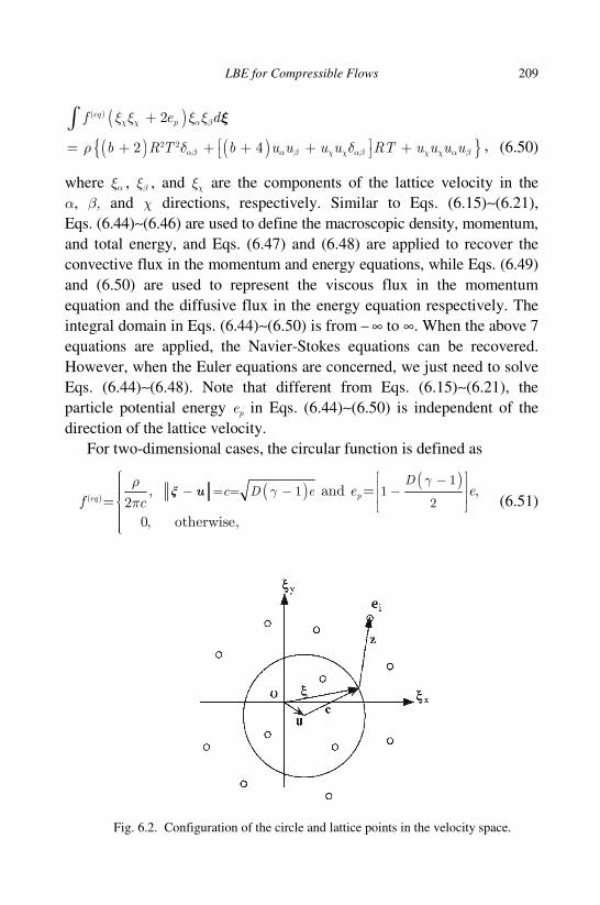
LBE for Compressible Flows 209
( )
( ) ( )
( )
2 2
2
2 4
eqpf e d
b R T b u u u u RT u u u u
ξ+
= + + + + +
∫ χ χ α β
αβ α β χ χ αβ χ χ α β
ξ ξ ξ ξ
ρ δ δ , (6.50)
where αξ , βξ , and χξ are the components of the lattice velocity in the
α, β, and χ directions, respectively. Similar to Eqs. (6.15)∼(6.21),
Eqs. (6.44)∼(6.46) are used to define the macroscopic density, momentum,
and total energy, and Eqs. (6.47) and (6.48) are applied to recover the
convective flux in the momentum and energy equations, while Eqs. (6.49)
and (6.50) are used to represent the viscous flux in the momentum
equation and the diffusive flux in the energy equation respectively. The
integral domain in Eqs. (6.44)∼(6.50) is from − ∞ to ∞. When the above 7
equations are applied, the Navier-Stokes equations can be recovered.
However, when the Euler equations are concerned, we just need to solve
Eqs. (6.44)∼(6.48). Note that different from Eqs. (6.15)∼(6.21), the
particle potential energy ep in Eqs. (6.44)∼(6.50) is independent of the
direction of the lattice velocity.
For two-dimensional cases, the circular function is defined as
( )
( )( )
1= = 1 1
2, and = ,
= 2
0, otherwise,
peq
Dc D e e e
f c
γγ
ρ
π
−− − −
uξ (6.51)
Fig. 6.2. Configuration of the circle and lattice points in the velocity space.

210 Lattice Boltzmann Method and Its Applications in Engineering
where e is the potential energy of the mean flow, which is defined as
e = p/(γ −1)ρ. The physical meaning of Eq. (6.51) is that all the mass,
momentum, and energy are concentrated on a circle as shown in Fig. 6.2.
The particle velocity on the circle can be written as
= +u cξ . (6.52)
Thus, the integral over the infinite domain of velocity space in
Eqs. (6.44)∼(6.50) reduces to the line integral along the circle, i.e.,
d ds cdθ= =ξ . (6.53)
Substituting Eqs. (6.51)∼(6.53) into Eqs. (6.44)∼(6.50), one can get
2( )
0 2eqf d cd
c
π ρθ ρ
π= =∫ ∫ξ , (6.54)
( )2
( )
0 2eqf d cd u
c
π
α αα
ρξ θ ρ
π= =+∫ ∫ u cξ , (6.55)
( ) ( ) ( )
( )
2( )
02 2
2
,
eqp pf e d cd e
c
u u bRT
π
α α
α α
ρξ ξ θ ρ
π
ρ
+ = + ⋅ + +
= +
∫ ∫ u c u cξ
(6.56)
( ) ( )2
( )
0 2eqf d cd u u p
c
π
α β α β αβα β
ρξ ξ θ ρ δ
π= = ++ +∫ ∫ u c u cξ , (6.57)
( )
2
0
( 2 )
( ) ( ) 2( )2
( 2) ,
eqp
p
f e d
cd e uc
u u b RT u
ξ+
= + ⋅ + ++ = + +
∫∫ u c u c u c
α α β
π
ββ
α α β
ξ ξ ξ
ρθ ρ
πρ
,
(6.58)
( ) ( ) ( )
( )
2( )
0 2
,
eqf d cdc
p u u u u u u
π
α β χ α β χ
α βχ β χα χ αβ α β χ
ρξ ξ ξ θ
π
δ δ δ ρ
= + + +
= + + +
∫ ∫ u c u c u cξ
(6.59)
( )
( )
2
0
2 2
( 2 )
= ( + ) ( + ) 2 ( + )( + ) ( + )2
4 .
eqp
p
f e d
cd e u u RTc
bR T b u u u u RT u u u u
χ χ α β
π
α β αβα β
αβ α β χ χ αβ χ χ α β
ξ ξ ξ ξ
ρθ ρ δ
π
ρ δ δ
+
⋅ +
= + + + +
∫
∫ u c u c u c u c
ξ
(6.60)

LBE for Compressible Flows 211
By comparing Eqs. (6.54)∼(6.60) with Eqs. (6.44)∼(6.50), it can be found
that only Eq. (6.60) has a little difference from Eq. (6.50) for the
coefficient of the first term on the right-hand side, which only affects the
heat conductivity.
6.3.2 Distribution of circular function to lattice points in
velocity space
It has been shown above that the circular function can satisfy the
constraints to recover the compressible Navier-Stokes equations.
However, the circular function cannot be directly applied in the LBE.
Although the circular function is greatly simplified as compared to the
Maxwellian distribution function, it is still a continuous function and the
integral in the velocity space is performed along the circle. In the context
of LBE, the discrete lattice velocity is specified, and the integral in the
relevant constraints is replaced by a summation over all lattice velocity
directions. It is expected that the equilibrium distribution function in a
lattice model can be obtained by distributing the circular function into
lattice points in the velocity space in such a way that the conservation
forms of moments (6.54)∼(6.60) can be satisfied in the context of LBE
when the integral is replaced by summation.
Suppose that in the ξx−ξy space, there are N lattice points, ei. As
shown in Fig. 6.2, the discrete velocity ei and the original velocity ξ have
the following relationship
i i= +e zξ . (6.61)
The continuous circular function is needed to be distributed to all
discrete points ei . For any dρ on the circle, it has a contribution ( )i dφ ρξ
at the discrete point ei , where ( )iφ ξ is the assigning function. Thus, the
contribution of the whole circle to ei can be written as
( ) 1( ) (2 ) ( )eqi i if d c dsφ ρ ρ π φ−= =∫ ∫ ξ ξ , (6.62)
where ( )eqif is the equilibrium distribution function in the ei direction. At
a physical position, the macroscopic density is the summation of all ( )eqif ,
i = 1, 2, …, N, that is
( ) 1 1
1 1 1
(2 ) ( ) (2 ) ( )N N N
eqi i i
i i i
f c ds c dsρ ρ π φ ρ π φ− −
= = =
= = =∑ ∑ ∑∫ ∫ ξ ξ . (6.63)

212 Lattice Boltzmann Method and Its Applications in Engineering
Equation (6.63) requires
( )1
N
i i
i
φ=
∑ ξ 1= . (6.64)
In a similar way, we can get the relationships
( )1
0N
i i
i
z αφ=
=∑ ξ , (6.65)
( )1
0N
i i i
i
z zα βφ=
=∑ ξ , (6.66)
( )1
0N
i i i i
i
z z zα β χφ=
=∑ ξ . (6.67)
Equations (6.64)∼(6.67) are actually the constrains for the assigning
function ( )iφ ξ . It was found that when the third-order Lagrange
interpolated polynomial is taken as the assigning function ( )iφ ξ , the
constraints (6.64)∼(6.67) can be satisfied. It is shown in [Qu et al., 2007a]
that, when 13 lattice points as shown in Fig. 6.3 are taken in the ξx−ξy
plane, the assigning function ( )iφ ξ can take the following form,
2 2 4 2 2 41( , ) 1 5 /4 5 /4 /4 /4x y x y x x y yφ = − − + + + , (6.68a)
2 3 2 4 2 22( , ) 2 /3 2 /3 /6 /2 /6 /2x y x x x xy x x yφ = + − − − − , (6.68b)
2 2 3 2 2 43( , ) 2 /3 2 /3 /2 /6 /2 /6x y y y x y y x y yφ = + − − − − , (6.68c)
2 3 2 4 2 24( , ) 2 /3 2 /3 /6 /2 /6 /2x y x x x xy x x yφ = − + + + − − , (6.68d)
2 2 3 2 2 45( , ) 2 /3 2 /3 /2 /6 /2 /6x y y y x y y x y yφ = − + + + − − , (6.68e)
2 2 2 26( , ) /4 /4 /4 /4x y yx x y xy x yφ = + + + , (6.68f)
2 2 2 27( , ) /4 /4 /4 /4x y yx x y xy x yφ = − + − + , (6.68g)
2 2 2 28( , ) /4 /4 /4 /4x y yx x y xy x yφ = − − + , (6.68h)
2 2 2 29( , ) /4 /4 /4 /4x y yx x y xy x yφ = − − + + , (6.68i)

LBE for Compressible Flows 213
2 3 410( , ) /12 /24 /12 /24x y x x x xφ = − − + + , (6.68j)
2 3 411( , ) /12 /24 /12 /24x y y y y yφ = − − + + , (6.68k)
2 3 412( , ) /12 /24 /12 /24x y x x x xφ = − − + , (6.68l)
2 3 413( , ) /12 /24 /12 /24x y y y y yφ = − − + , (6.68m)
where x and y are lattice velocity components in the ξx and ξy directions
respectively. Once the assigning function is obtained, the equilibrium
distribution function at the i-th lattice point can be evaluated as
( ) 1(2 ) ( ) , 1, 2, ... , 13eqi if c ds iρ π φ−= =∫ ξ . (6.69)
Substituting Eq. (6.68) into Eq. (6.69) gives
()
( ) 4 4 2 2 2 41
2 2 2 2 2 2
4 5 20 16 16 416
20 20 20 20 ,
eqf u c c u v v
v c v c u u
ρ= + − + + +
− + + −
(6.70a)
()
( ) 2 4 4 2 2 2 22
2 2 2 2 2 3
16 3 4 8 6 1224
18 12 12 16 4 ,
eqf u c u c c v uv
c u c u u v u u
ρ= − − + + − + +
+ + + − +
(6.70b)
()
( ) 2 2 2 2 2 2 2 23
4 2 4 2 3
12 6 18 12 1224
3 8 4 16 4 16 ,
eqf u v c u c v c v u v
c c v v v v
ρ= − + + + +
+ − + − + −
(6.70c)
()
( ) 2 4 4 2 2 2 24
2 2 2 2 2 3
16 3 4 8 6 1224
18 12 12 16 4 ,
eqf u c u c c v uv
c u c u u v u u
ρ= − − + + − + −
+ − + + −
(6.70d)
()
( ) 3 2 2 4 2 45
2 2 2 2 2 2 2
4 12 12 3 8 424
16 16 12 18 6 ,
eqf v c v u v c c v
v v u v c v c u
ρ= − − − − + − +
− + + + +
(6.70e)
()
( ) 2 2 2 26
4 2 2 2 2 2 2
8 8 4 4 832
8 4 4 ,
eqf uv vu c u c v u v
c u v c v c u
ρ= + + + +
+ + + +
(6.70f)

214 Lattice Boltzmann Method and Its Applications in Engineering
()
( ) 4 2 2 2 27
2 2 2 2 2 2
4 8 8 432
4 4 8 8 ,
eqf c c v uv vu c u
c u c v u v u v
ρ= + − − +
− + + +
(6.70g)
()
( ) 4 2 2 2 28
2 2 2 2 2 2
4 8 8 432
4 4 8 8 ,
eqf c c v uv vu c u
c u c v u v u v
ρ= − − + +
− + + −
(6.70h)
()
( ) 4 2 2 2 29
2 2 2 2 2 2
4 8 8 432
4 4 8 8 ,
eqf c c v uv vu c u
c u c v u v u v
ρ= − + − +
+ + + −
(6.70i)
()
( ) 4 3 2 2 210
2 2 4
8 16 8 16 24192
24 4 3 ,
eqf u u u u c u
c u c c
ρ= + − − +
+ − +
(6.70j)
u
c
1
2
3
4
5
6
7
89
10
11
12
13
(0,1)
(0,-1)
(1,0)(-1,0)(-2,0) (2,0)
(0,-2)
(0,2)
( )2, 2( )− 2, 2
( )− −2, 2
( )−2, 2
Fig. 6.3. Configuration of 13 lattice points in the -x yξ ξ plane.

LBE for Compressible Flows 215
()
( ) 2 2 4 211
2 2 3 4
16 24 8 8 4192
24 16 3 ,
eqf v c v v v c
c v v c
ρ= − + − + −
+ + +
(6.70k)
()
( ) 4 3 2 2 212
2 2 4
8 16 8 16 24192
24 4 3 ,
eqf u u u u c u
c u c c
ρ= − − + +
− − +
(6.70l)
()
( ) 2 2 4 213
2 2 3 4
16 24 8 8 4192
24 16 3 ,
eqf v c v v v c
c v v c
ρ= − − + −
+ − +
(6.70m)
where u and v are the velocity components of u.
Note that Eq. (6.70) is formed in the ξx−ξy plane. No particle potential
energy has been considered. Next, we will use the same distribution
process to assign the potential energy to each lattice point. As ep is
linearly appeared in Eqs. (6.54)∼(6.60), it means that only two energy
levels are needed. As shown in Fig. 6.4, two energy levels, λ1 = 0 and
λ2 > ep, are assigned. At each energy level, there are 13 lattice points (the
configuration of these lattice points is shown in Fig. 6.3). So, there are
26 lattice points in total, and this lattice model is termed as D2Q13L2
model.
ξξξξy
ξξξξx
λ
O
epu c
λ2
Fig. 6.4. Configuration of lattice points on two energy levels.

216 Lattice Boltzmann Method and Its Applications in Engineering
With the particle potential energy λ1 = 0 and λ2 at two energy levels,
the summation form of Eq. (6.56) can be written as
( ) ( ) ( )2
( ) ( )
1 1 1
2 2N N
eq eqi i i p iv i i v
i i v
u u bRT f e e e f e eα α α α α αρ λ= = =
+ = + = +∑ ∑∑ (6.71)
where ( )1eq
if and ( )2eq
if are the equilibrium distribution functions associated
with energy levels of λ1 and λ2 . By unwrapping Eq. (6.71), one can get
( ) ( ) ( )1 1 2 2
( ) ( ) ( )1 2
,
.
eq eq eqi p i i
eq eq eqi i i
f e f f
f f f
λ λ = + = +
(6.72)
Thus, the final expression of the equilibrium distribution function ( )eqivf
can be written as
2( ) ( )1
2 1
1( ) ( )2
2 1
,
.
peq eqi i
peq eqi i
ef f
ef f
λ
λ λ
λ
λ λ
− = − − = −
(6.73)
As λ1 = 0 and λ2 can be taken as 1 from normalization, Eq. (6.73) can be
finally simplified to
( ) ( )1
( ) ( )2
(1 ),
.
eq eqi i p
eq eqi i p
f f e
f f e
= − =
(6.74)
Note that the above D2Q13L2 model is only applicable for simulation
of inviscid flows. It also encounters numerical instability when the
streaming-collision process is applied. Thus, it should be combined with
the solution of DVBE, which will be discussed in Section 6.6. For
simulation of one-dimensional inviscid flows such as shock tube
problems or application of LBE to evaluate inviscid flux at the cell
interface in the solution of Euler equations, Qu et al. [2007a] also
presented a one-dimensional model, D1Q5L2, which is shown below.
For the one-dimensional case, the circular function is reduced to the
following form
( ) ( )( )
11 and 1 1 .
2
, otherwise.
, 2
0
peq
e e ef
γ γρ
| − |= = − = − − =
u cξ
(6.75)

LBE for Compressible Flows 217
The equilibrium distribution functions at 5 lattice points, ei=0, d1, −d1,
d2, −d2 , are given by
2 2 2 2 2 2 2 2 2 2 4 2 2 41 2 1 1 2 2( )
1 2 21 2
6eq
d d d u d c d u d c u u c cf
d d
ρ
− − − − + + += , (6.76a)
2 2 2 2 2 2 2 2 4 4 31 1 2 2 2 1( )
2 2 2 21 1 2
3 6
2
eqd uc d d u d u d c u c c u d u
fd d d
ρ
− − − + + + +=
−, (6.76b)
2 2 2 2 2 2 2 2 4 4 31 2 1 2 2 1( )
3 2 2 21 1 2
3 6
2
eqd d u d uc d u d c u c c u d u
fd d d
ρ
− − − + + + −=
−, (6.76c)
2 2 2 2 2 2 2 2 4 4 32 1 2 1 1 2( )
4 2 2 22 1 2
3 6
2
eqd d u d uc d u d c u c c u d u
fd d d
ρ
− + + − − − −=
−, (6.76d)
2 2 22 2 2 2 2 4 4 32 2 21 1 1( )
5 2 2 2
2 1 2
3 + + 6=
2
eqd uc d u u c u c c u d ud d d
fd d d
ρ
− − − − +
−, (6.76e)
where 1d and 2d can be taken as d1 = 1 and d2 = 2. Finally, we can use
Eq. (6.74) to calculate the equilibrium distribution functions at the lattice
points of each energy level.
Qu et al. [2007a, 2007b] successfully applied the above models to the
one-dimensional shock tube problems, the two-dimensional shock
reflection on the wall, and the double Mach reflection as well as shock
wave propagation in an enclosure. After initial work of Qu et al. [2007a,
2007b], Li et al. [2009] further improved the model, where a three-
dimensional circular function (spherical function) is used to construct a
D3Q25 model for simulation of inviscid compressible flows.
6.4 Delta Function-based LBE Models for Compressible
Flows
Also aiming at the simulation of compressible flows, Sun [1998, 2000a,
2000b] and Sun and Hsu [2003, 2004] developed an adaptive lattice
Boltzmann model. Unlike the compressible lattice Boltzmann models
shown above, the adaptive lattice Boltzmann model is based on a simple

218 Lattice Boltzmann Method and Its Applications in Engineering
delta function. The pattern of the lattice velocities of this model varies
with mean flow velocity and internal energy. The adaptive lattice
Boltzmann model contains several discrete velocity vectors which are
symmetrically located around the mean velocity in the velocity space.
And density is equally distributed on all the discrete velocity vectors.
Let x be an arbitrary node of a lattice, ( , , , , , )f m tζx r ξ be the density
distribution function for the particle with the migrating velocity r,
moving to t+ ∆x r during t∆ , and transporting the mass m, velocity ξ,
and energy ζ. Let D ζ= ×ξ be a set of the phase velocity ξ, and
phase energy ζ, S = r be a set of migrating velocity. Then the
macroscopic conservative variables can be defined as
( ), , , , ,D
S
mf m t dmd dρ ζ ζ∈
≡ ∑∫r
x r ξ ξ , (6.77)
( ), , , , ,D
S
f m t dmd dρ ζ ζ∈
≡ ∑∫r
v x rξ ξ ξ , (6.78)
( ), , , , ,D
S
E f m t dmd dρ ζ ζ ζ∈
≡ ∑∫r
x r ξ ξ . (6.79)
If we define
, ,m ζ ≡ ξηηηη , (6.80)
(x, r, , ) (x, r, , , , )f t f m tζ≡η ξη ξη ξη ξ , (6.81)
Y , , Eρ ρ ρ ≡ v , (6.82)
Eqs. (6.77)∼(6.79) can be written in a compact form as
( )Y , , ,D
S
f t d∈
≡ ∑∫r
x rη η ηη η ηη η ηη η η . (6.83)
As shown in Fig. 6.5, suppose that we consider a hexagonal lattice with
lattice velocity set as
c ; 1,2,..., 6, 1,2jv vj b v′ = = = . (6.84)
In the adaptive LBE model, the total mass, momentum and energy are all
transported by the particle velocity, cjvk, which is defined as,
jvk k jv′= +c v c , (6.85)

LBE for Compressible Flows 219
where vk is the approximated fluid velocity at a mesh point. Consider an
arbitrary node x, where its fluid velocity is v. As shown in Fig. 6.6, the
node x should fall into one of triangles. We note this triangle as ∆ABC.
The approximated fluid velocity at nodes A, B and C are noted as v1, v2
and v3. The particle velocity at x and the approximated fluid velocity vk
are defined as
jv jv′= +c v c , (6.86)
k k′= +v v v . (6.87)
In the adaptive LBE model, all the particles are concentrated at
jvk=r c , jvkm m= , jvk=ξ ξξ ξξ ξξ ξ , jvkζ ζ= , and the equilibrium distribution
function can be written as
( )( ) ( ) ( )
( ) , ,
, ,
0, other ,
eqjvk
vk jvk jvk jvk jvk
f t
d m m
S
δ δ δ ζ ζ − − − =≡ ∈
x
r c
r
ξ ξ
ηηηη
(6.88)
where δ is the delta function, ( ) 0δ =ξ for ξ ≠ 0; ( ) ( )( ) ( ) (0)eq eqf d fδ =∫ ξ ξ ξ .
vkd is a function of macroscopic variables. With Eq. (6.88), the
macroscopic variables can be determined as
, ,
vk jvk
j v k
d∑Y = ηηηη , (6.89)
where [ , , ]jvk jvk jvk jvkm ζ≡ ξηηηη . Sun [2000a] proposed two models to compute
the particle mass, velocity, and energy. Model I gives
1Ijvkm = , (6.90)
Ijvk jv= cξξξξ , (6.91)
''''11111111cccckvvvv ''''21212121cccc''''31313131cccc''''41414141cccc ''''51515151cccc ''''61616161cccc
Fig. 6.5. Configuration of fluid velocity and a symmetric set of velocities.

220 Lattice Boltzmann Method and Its Applications in Engineering
2 21( 2 )
2Ijvk jv vv cζ ′ ′= + ⋅ + + Φc v , (6.92)
, ,T
I I I Ijvk jvk jvk jvkm ζ ≡ ξηηηη , (6.93)
where Φ is the particle potential energy,
1 ( 1)2
Deγ
Φ = − −
. (6.94)
Model II introduces corrections to Model I, and it is given as
II Ijvk jvk jvkm m χ= − , (6.95)
II Ijvk jvk jvkχ= − vξ ξξ ξξ ξξ ξ , (6.96)
2 21( )
2II Ijvk jvk jvk v cζ ζ χ
′= − + + Φ
, (6.97)
, ,T
II II II IIjvk jvk jvk jvkm ζ ≡ ξηηηη , (6.98)
where 2 1(2 ) ( )jvk v jv kD cχ −′ ′ ′= ⋅c v . With the introduction of density portion,
/k kα ρ ρ= , vkd can be taken as
vk k vd dα= . (6.99)
As shown in Fig. 6.6, with the given location x, it is not difficult to
calculate the density portion. For the hexagonal lattice, there are two
levels of v′c . Then d1 and d2 in Eq. (6.99) can be determined by
2
21 2 2
1 2 1
( 1)
( )
c D ed
b c c
γρ
′ − −=
′ ′−, (6.100)
2
12 2 2
2 2 1
( 1)
( )
D e cd
b c c
γρ
′− −=
′ ′−. (6.101)
In order to ensure the positivity of d1 and d2 , 1c ′ and 2c ′ are required to
satisfy 2 21 2( 1)c D e cγ′ ′< − < . In practice, 1c ′ is set to be the integer part
of ( 1)D eγ − , and 2 1 1c c′ ′= + . When 1 0c′ = , the correction parameter
in Eqs. (6.95)∼(6.97) should be modified to
1 21 2 22
2 2
0, ( )2
j k j k j k
d d D
d cχ χ
+ ′ ′= = ⋅′c v . (6.102)

LBE for Compressible Flows 221
The pressure in the adaptive LBE can be computed by
21v v v
v
p b d cD
′= ∑ . (6.103)
In the application of adaptive LBE, the relaxation parameter τ is usually
set as one due to huge requirement of computer memory and
computational effort for other cases. When τ = 1, the lattice Boltzmann
equation is reduced to
( )( , , , ) ( , , , )eqf t t t f t+ ∆ + ∆ =x r r x rη ηη ηη ηη η . (6.104)
Some compressible flows with weak or strong shock waves were
simulated successfully by the adaptive LBE. Note that since the viscosity
cannot be adjusted by changing τ, the model can only be used to simulate
inviscid flows if the viscosity terms are regarded as numerical
dissipation.
6.5 Direct Derivation of Equilibrium Distribution Functions
from Conservation of Moments
All of the LBE models described above are based on a given form of
equilibrium distribution functions. On the other hand, it was found that
the equilibrium distribution functions can also be derived from the
Fig. 6.6. Illustration of fluid velocity at x and its approximated velocity at apexes of a
triangle.

222 Lattice Boltzmann Method and Its Applications in Engineering
conservation forms of moments. The initial work was made by
McNamara et al. [1995] and Dellar [2008]. In the work of McNamare
et al. [1995], a system of 21 moment conservation equations is used to
determine the distribution functions of thermal lattice Boltzmann model.
Later, Dellar [2008] derived two one-dimensional models, unsplit 7
velocity model and split 4+3 velocity model, by solving a linear system
of 7 moment conservation equations. In the following, the unsplit 7
velocity model is briefly described.
This model chooses 7 lattice velocities as ξi = i, i = 0, ±1, ±2, ±3.
With the introduction of a particle potential energy εi/2, the 7
conservation forms of moments can be written as
3( )
3
eqi
i
f ρ=−
=∑ , (6.105)
3( )
3
eqi i
i
f uξ ρ=−
=∑ , (6.106)
3( )2 2
3
eqi i
i
f uξ ρθ ρ=−
= +∑ , (6.107)
3( )3 3
3
3eqi i
i
f u uξ ρ ρ θ=−
= +∑ , (6.108)
( )3
( )2 2
3
1 1
2 2 1
eqi i i
i
f uρθ
ξ ε ργ=−
+ = +−∑ , (6.109)
( )3
( )2 3
3
1 1
2 2 1
eqi i i i
i
f u uγ
ξ ε ξ ρ ρ θγ=−
+ = +−∑ , (6.110)
( )3
( )2 2 4 2 2
3
5 1
2 1
1 1
2 2 1
eqi i i i
i
f u uγ
γξ ε ξ ρ ρ θ ρθ
γ=−
+−
+ = + + −∑ , (6.111)
where θ is proportional to the temperature T, and θ =RT. Note that
although different notations are used, Eqs. (6.105)∼(6.111) are actually
the one-dimensional forms of Eqs. (6.15)∼(6.21). By taking εi = (0, 0, 1,
4, 1, 0, 0), equations. (6.105)∼(6.111) can be put in the following matrix

LBE for Compressible Flows 223
form,
( )3
( )2
( )1
( )0
( )1
( )2
( )3
1 1 1 1 1 1 1
3 2 1 0 1 2 3
9 4 1 0 1 4 9
27 8 1 0 1 8 27
9 4 2 4 2 4 9
27 8 2 0 2 8 27
81 16 2 0 2 16 81
eq
eq
eq
eq
eq
eq
eq
f
f
f
f
f
f
f
−
−
−
− − −
− − −
− − −
4 2
2
2
3
2
3
2 /( 1)
5 3
1
3=
2 /( 1)
2 /( 1)
( )
u
u
u
u
u u
u
u u
θ γ γ
θ γ
θ
θρ
θ γ
θ γ γ
−
+ −
+ + + − + − +
. (6.112)
The solution of equation system (6.112) can be obtained analytically. For
example, the equilibrium distribution function of static particle is
( ) 2 4 2 20
12 62 5 3 2= 36 13
64 1 1 1
eqf u u uρ γ γ γ
θ θ θγ γ γ
− − − + − − − − − − −. (6.113)
Recently, Yang et al. [2012] did a systematic study on derivation of
one-dimensional lattice Boltzmann models from conservation forms of
moments in order to simulate compressible inviscid flows. As discussed
in the previous sections, for the inviscid flow, only 5 conservation forms
of moments are needed. Their one-dimensional forms can be written as
( )eqi
i
fρ = ∑ , (6.114)
( )eqi i
i
u fρ ξ= ∑ , (6.115)
( )2 eqi i i
i
u p fρ ξ ξ+ = ∑ , (6.116)
( ) ( )2 2eq eqi i i i
i i
u bRT f fρ ξ ξ λ+ = +∑ ∑ , (6.117)
( ) ( ) ( )2 2 2eq eqi i i i i i
i i
u b RT u f fρ ξ ξ ξ λ ξ + + = + ∑ ∑ , (6.118)
where b is defined by Eq. (6.22), and λ is the particle potential energy.
Note that different from other LBE models [Kataoka, T. and Tsutahara,
2004a, 2004b; Dellar, 2008], the particle potential energy in Eqs. (6.117)
and (6.118) is independent of the lattice velocity direction i. This is
reasonable as the particle potential energy reflects the contribution of

224 Lattice Boltzmann Method and Its Applications in Engineering
kinetic energy in the rotational velocity space, which is independent of
translational velocity space. Unlike the previous work [Kataoka, T. and
Tsutahara, 2004a, 2004b; Dellar, 2008], the particle potential energy λ in
Eqs. (6.114)∼(6.118) cannot be arbitrarily specified. In fact, it can be
determined from the equation system. By substituting Eqs. (6.114) and
(6.116) into Eq. (6.117), one can get the expression of λ as
( )
( )1
1 12 2
b DRT eλ γ
− = = − −
. (6.119)
Due to the use of Eq. (6.119), only 4 equations of (6.114)∼(6.118) are
independent, which can be written as
( )eqi
i
fρ = ∑ , (6.120)
( )eqi i
i
u fρ ξ= ∑ , (6.121)
( )2 2 eqi i i
i
u c fρ ρ ξ ξ+ = ∑ , (6.122)
( )3 23 eqi i i i
i
u uc fρ ρ ξ ξ ξ+ = ∑ , (6.123)
where c is the peculiar velocity of particles defined as ( 1)c D eγ= − .
When the lattice velocities are taken as ξi =0, ±d1, ±d2, where d1 and
d2 are constants, there are 5 unknowns, ( ), 1, 2, ..., 5eqif i = . As equation
system (6.120)∼(6.123) only has 4 equations, we have to regard one of ( )eqif as given in order to obtain a well-posed equation system. If we set ( )1eqf as known, we can get the solution of equation system (6.120) ∼
(6.123) as
( )( ) ( )1 1 , ,eq eqf f u cρ= , (6.124)
( )( ) 2 2 2 2 3 21 1 2 2 1 1( )
2 2 21 1 2
3
2
eq
eqf d d d u d u d c u uc
fd d d
ρ ρ ρ ρ ρ ρ
− − − + + + +=
−, (6.125)
( )( ) 2 2 2 2 3 21 1 2 2 1 1( )
3 2 21 1 2
3
2
eq
eqf d d d u d u d c u uc
fd d d
ρ ρ ρ ρ ρ ρ
− − + + + − −=
−, (6.126)
( )( ) 2 2 2 2 3 21 1 2 1 2 2( )
4 2 22 1 2
3
2
eq
eqf d d d u d u d c u uc
fd d d
ρ ρ ρ ρ ρ ρ
− + − − − −=
−, (6.127)

LBE for Compressible Flows 225
( )( ) 2 2 2 2 3 21 1 2 1 2 2( )
5 2 22 1 2
3
2
eq
eqf d d d u d u d c u uc
fd d d
ρ ρ ρ ρ ρ ρ
− − − − + +=
−. (6.128)
In fact, if we take ( )1eqf as the following form,
( )2 2 2 2 2 2 2 2 2 2 4 2 2 41 2 1 1 2 2( )
1 2 21 2
6eq
d d d u d c d u d c u u c cf
d d
ρ − − − − + + += , (6.129)
we can get exactly the same results as D1Q5L2 model of Qu et al. [2007]
given by Eq. (6.76). Furthermore, when 4 lattice velocities are taken, that
is, ξi =±d1, ±d2, the equation system (6.120)∼(6.123) gives the 4
equilibrium distribution functions as
2 2 2 2 3 21 2 2 1 1( )
1 2 21 1 2
3
2eq
d d d u d u d c u ucf
d d d
ρ
− − + + + +=
−, (6.130)
2 2 2 2 3 21 2 2 1 1( )
2 2 21 1 2
3
2eq
d d d u d u d c u ucf
d d d
ρ
− + + + − −=
−, (6.131)
2 2 2 2 3 21 2 1 2 2( )
3 2 22 1 2
3
2eq
d d d u d u d c u ucf
d d d
ρ
+ − − − −=
−, (6.132)
2 2 2 2 3 21 2 1 2 2( )
4 2 22 1 2
3
2eq
d d d u d u d c u ucf
d d d
ρ
− − − + +=
−. (6.133)
The equation system (6.120)∼(6.123) is a useful platform to derive
various one-dimensional LBE models for compressible inviscid flows.
6.6 Solution of Discrete Velocity Boltzmann Equation
The application of lattice Boltzmann models for simulation of compress-
ible flows often encounters numerical instability. To obtain a stable
solution, very few of existing models such as those of Yan et al. [1999]
and Yu and Zhao [2000] can be applied with normal streaming-collision
process. Most of existing models have to be applied with the solution of
DVBE (6.2). In fact, in the literature, there are many works [Chew et al.,
2002; Gan et al., 2008; Li et al., 2007; Li et al., 2009; Mei and Shyy,

226 Lattice Boltzmann Method and Its Applications in Engineering
1998; Mezrhab et al., 2004; Peng et al., 1999; Watari, M. and Tsutahara,
2003] available to address the solution of DVBE for problems with
complex geometry, thermal flows, and compressible flows. Some
techniques for solving the DVBE for compressible flows are described in
this section.
To apply their compressible LBE models, Kataoka and Tsutahara
[2004] solved the DVBE by the following Crank-Nicolson scheme,
( )
2
eqi i i i i
i it t tt t t t
c t f f f ff f t
x x
α
α α τ+∆+∆
∆ ∂ ∂ − = − + + ∆ ∂ ∂ , (6.134)
where ∆t is the time step. The spatial derivatives if xα∂ ∂ can be
approximated by the following second-order upwind scheme,
3 ( ) 4 ( ) ( 2 ) (2 ), 0,=
3 ( ) 4 ( ) ( 2 ) (2 ), 0.
i i i ii
i i i i
f x f x x f x x x cf
x f x f x x f x x x c
α α α α
α α α α α
− − ∆ + − ∆ ∆ ≥∂ ∂ − + + ∆ − + ∆ ∆ < (6.135)
Kataoka and Tsutahara [2004] found that the application of Eqs. (6.134)∼
(6.135) with t τ∆ ∼ and x RTτ∆ ∼ can obtain stable solutions with
the second-order of accuracy. The DVBE can also be solved by some
powerful flux solvers such as MUSCL which are often used to solve the
Euler equations. For a two-dimensional case, Qu et al. [2007] wrote
Eq. (6.2) into the following conservative form
f F G
t x y
α α αα
∂ ∂ ∂+ + = Ω
∂ ∂ ∂, (6.136)
where
eq
x y
f fF f c G f c α αα α α α α α α
τ
−= , = ,Ω = − . (6.137)
As i will be used as the index to indicate x-coordinate, we have used α in
Eqs. (6.136) and (6.137) to replace i in Eq. (6.2). Using the explicit Euler
scheme for temporal discretization and finite volume method for spatial
discretization, Eq. (6.136) can be discretized as
1 1 1 12 2 2 2
1 1 1= +
n nn n n n n
i ji j i j i j i j
f fF F G G
t x y
α ααα α α α
+ , ,, + , , − , , , + , , −
−− − − − Ω
∆ ∆ ∆, (6.138)

LBE for Compressible Flows 227
where 1/2ni jFα, ± , and 1/2
ni jGα, , ± are the numerical fluxes at the interfaces of a
cell (i, j). In order to compute the numerical fluxes, the 3-rd order
MUSCL (Monotone Upstream-centered Scheme for Conservation Laws)
scheme [van Leer, 1982] with van Albada limiter [1982] is applied to
evaluate the functional value on two sides of an interface
( ) ( )
( ) ( )
12
12
1
1
1 1 ,4
,1 14
L iii
iR ii
sf f s s
sff s s
κ κ
κ κ
− + + + + − + +
= + − ∆ + + ∆
= − − ∆ + + ∆ (6.139)
where κ = 1/3, and s is the van Albada limiter given by
2 2
2s
ε
ε
+ −
+ −
∆ ∆ +=
∆ + ∆ +. (6.140)
Here ε is a small number (usually set as 610ε −= ) preventing division by
zero in region of null gradient and
1i iif f
+ + ∆ = − , 1i iif f
− − ∆ = − . (6.141)
With 1/2( )L if + and 1/2( )R if + , the numerical flux at the interface i + 1/2 can
be computed with a Riemann solver. For Eq. (6.136), the exact Riemann
solution can be found since it is a linear hyperbolic system. The solution
is
1/21/2
1/2
, if 0,
, if 0.
L x xii
R x xi
f c cF
f c c
++ +
>= < (6.142)
1/2ni jGα, , ± can be evaluated in the same way.
Note that when the DVBE is solved by the upwind schemes, the
artificial dissipation comes from two parts. One is the model dissipation
which is from the collision term. This part is usually very small. The
other is the numerical dissipation resulted from spatial discretization.
Numerical results have shown that the solution of the DVBE by upwind
schemes with associated compressible LBE models can well capture both
the shock waves and contact discontinuities without oscillation.

228 Lattice Boltzmann Method and Its Applications in Engineering
6.7 Lattice Boltzmann Flux Solver for Solution of Euler
Equations
As shown in previous sections, the developed lattice Boltzmann models
for compressible flows are usually very complicated, especially for two-
and three-dimensional cases. And the compressible LBE models are
often associated with the solution of DVBE, which may encounter
numerical instability. To overcome these drawbacks, some efforts
[Ji et al., 2009; Joshi et al., 2010; Yang et al., 2012] have been made to
combine one-dimensional compressible LBE models with the solution of
the Euler equations by the finite volume method (FVM). In other words,
the one-dimensional models are used to the local Riemann problem at the
cell interface to evaluate the inviscid flux. The work is actually an
inviscid flux solver by the lattice Boltzmann method. In this section, we
will briefly describe how to apply the one-dimensional LBE model to
evaluate the inviscid flux at a cell interface for one-dimensional and two-
dimensional problems.
For simplicity, we first consider the one-dimensional case, for which
the Euler equations can be written as
0t x
∂ ∂+ =
∂ ∂W F
, (6.143)
where
2
2 2
,
[ ] [ ( 2) ]2 2
u
u u p
u bRT u b RT u
ρ ρ
ρ ρ
ρ ρ
+ = = + + +
W F . (6.144)
Using FVM, Eq. (6.143) can be discretized as
1/2 1/2
1( )i
i i
i
d
dt x+ −= − −
∆W
F F . (6.145)
4 2 1
2d− 1
d− 2d
1d
3
Fig. 6.7. Configuration of a D1Q4 lattice Boltzmann model.

LBE for Compressible Flows 229
Here Fi+1/2 is the inviscid flux at the cell interface i + 1/2. Conventionally,
Fi+1/2 can be evaluated by certain upwind schemes such as the Roe
scheme [Roe, 1981]. In the following, we will show that Fi+1/2 can also
be evaluated by the compressible LBE model.
For illustration, we consider a D1Q4 lattice Boltzmann model as
shown in Fig. 6.7. This model will be applied to a local Riemann
problem at the interface, which is shown in Fig. 6.8, where the flow
variables are constants at the left and right sides.
Now, at the interface, suppose that there are two neighbouring points
L and R located respectively at the left and right sides of the interface.
We apply the D1Q4 model to the points L and R at the time t. Since
macroscopic variables at points L and R are known, we initialize the
computation by using their equilibrium distribution functions. After a
time step ∆t, the particles 1 and 3 from point L and particles 2 and 4
from point R will stream to the interface. The streaming process is
demonstrated in Fig. 6.9.
Fig. 6.9. Streaming process of D1Q4 model near the interface.
Fig. 6.8. Sketch of a local Riemann problem.
, ,L L Lu pρ
interface
, ,R R Ru pρ
( ),
2
eq Lf ( ),
3
eq Lf
,
3
eq Rf( ),
4
eq Rf ( ),
2
eq Rf
( ),
1
eq Lf( ),
2
eq Rf( ),
4
eq Rf
L R L R
streaming ( ),
1
eq Lf
( ),
1
eq Rf
( ),
4
eq Lf
interface interface
( ),
3
eq Lf

230 Lattice Boltzmann Method and Its Applications in Engineering
From the streaming process, we have the density distribution
functions at the interface as follows,
( ), ( ), ( ), ( ),1 1 2 2 3 3 4 4, , , eq L eq R eq L eq Rf f f f f f f f= = = = . (6.146)
With Eqs. (6.146), (6.115)∼(6.118), the inviscid flux F at the interface
can be calculated by
12
2
23
1
1
1
[ ( 2) ]122
N
i i
iN
i i i
iN
i i i
i
i
uF
u pF
F u b RT ud d
d
d
f
f d d
f
ρ
ρ
ρ
λ
=
=
=
+ = = = + + + ∑
∑
∑F , (6.147)
where N is taken as 4 in Eq. (6.147) for the D1Q4 model. When multi-
dimensional problems are considered, the above 1D model needs to be
applied along the normal direction of interface. For example, for the 2D
case, as shown in Fig. 6.10, we can use the normal velocity Un to replace
u in the 1D model (6.147). Suppose that the unit normal vector at the
interface is (nx, ny) for the 2D case, we will have the following
relationships,
, n x y x yU n u n v U n v n u= + = −τ , (6.148)
, x n y x y nu n U n U v n U n Uτ τ= − = + , (6.149)
where Un and Uτ are the normal and tangential velocity components at
the interface, and u and v are the velocity components in the x and y
directions, respectively. The two-dimensional Euler equations can be
Fig. 6.10. Illustration of normal and tangential velocities at an interface.
nU
Uτ
v
u
interface

LBE for Compressible Flows 231
written as
0yx
t x y
∂∂ ∂+ + =
∂ ∂ ∂
FW F, (6.150)
where
2 2[2
]
u
v
u v
bRT
ρ
ρ
ρ
ρ
= + +
W ,
2
2 2[2( 2) ]
x
u
u p
uv
u v
b RT u
ρ
ρ
ρ
ρ
+ = + + +
F , 2
2 2[2( 2) ]
y
v
uv
v p
u v
b RT v
ρ
ρ
ρ
ρ
+ = + + +
F . (6.151)
Integrating Eq. (6.150) over a control volume I gives
1
1 fN
Ini i
iI
dS
dt V =
= − ∑WF , (6.152)
where WI is the vector of conservative variables for the control cell I, VI ,
and Nf are the volume and the number of faces of the cell, respectively,
and Si is the area of the i-th face of the control cell. The flux vector at the
interface is given by
2 2[ ( 2) ]2
n
n x
n x x y y n y
n
U
U u pn
n n U v pn
U u v b RT
ρ
ρ
ρ
ρ
+ = + = + + + +
F F F . (6.153)
Using Eq. (6.149), equation (6.153) can also be written as
( )( )
2 2
2
0
( 2)2
n
n
n n x n y
n n n y n x
n nU
U
U U p n U U n
U U p n U U n
U b RT U U
τ
τ
τ
ρ
ρ
ρ ρ
ρ ρ
ρ
+ − = ++ + +
F . (6.154)
Note that in the last component of the flux vector in Eq. (6.154), we have
used the relationship of 2 2 2 2nu v U U τ+ = + (velocity magnitude does not

232 Lattice Boltzmann Method and Its Applications in Engineering
change). If we define 1 1N
n i iiF U f d== = ∑ρ , and apply the one-dimensional
results of Eq. (6.147) to the normal direction, the flux vector at the
interface (Eq. (6.154)) can be finally written as
1
1
12
31
4
21
1
1
1
(- )
( )
1 1
2 2
N
i i
iN
i i i x y
iN
i
n
N
i
i i
i i
y
i
i
i
x
FF
F
FF
F
d
f d
f d d n
d
U n
f d d n
d
U
F
n
f U
τ
τ
τ
λ
=
=
=
=
= = + +
⋅ + ⋅ ⋅
⋅ + ⋅ ⋅
⋅∑
∑
∑
∑F
. (6.155)
In the above equations, the tangential velocity Uτ is still unknown. One
feasible way to calculate the terms of 1F τ⋅U and 21F U τ⋅ is given by
1 1 1L L R RF F U F UU τ τ τ+⋅=⋅ ⋅ , (6.156)
( ) ( )2 22
1 1 1L L R RF U F U F Uτ τ τ⋅ = ⋅ + ⋅ , (6.157)
where LU τ and RU τ are the tangential velocities at the two sides of the
interface. 1LF and 1
RF denote the mass fluxes calculated by the
equilibrium distribution functions (only consider the components
pointing to the interface) at the two sides of the interface. When
the D1Q4 model is applied, we have ( ), (1 21
),1 3
eq L LL eqf d f dF += and ( ), ( ),2 41 1 2eq R eR q Rf d f dF −= − . Once the flux vector at the interface is obtained
from Eq. (6.155), we can simply solve Eq. (6.152) by multi-stage Runge-
Kutta methods. The above process can also be easily extended to the
three-dimensional case.
6.8 Some Sample Applications
In the previous sections, a number of LBE models have been described
for compressible flows. In this section, we will show some sample
applications of these models.
One-dimensional case
Almost all the compressible LBE models introduced in the previous
sections can be used to simulate the one-dimensional shock tube

LBE for Compressible Flows 233
problems. Here, we only show some results of Qu et al. [2007] by using
their developed D1Q5L2 model. The initial condition of the Sod shock
tube problem is
( )
( )
1 0 2 5 , 0 5 0,
0 125 0 2 , 0 0 5.
L L L
R R R
u e x
u e x
ρ
ρ
, , = , , . − . < <
, , = . , , < < . (6.158)
For the simulation, Qu et al. [2007] set d1 = 1, d2 = 2, 4ˆ 10τ ε −= = . The
reference density and length are taken as ρ0 = 1, L0 = 1, and the reference
internal energy is chosen as e0 = 4 > max(e) = 2.5. Here, e is the internal
energy. The mesh size is taken as ∆x = 1/200 and the time step size is
chosen as ∆t = ε/4. Before the waves propagate to the two boundary
points, the distribution functions at the boundary are set as the
equilibrium distribution functions computed from the initial value of
macroscopic variables. The computed density, velocity, pressure, and
internal energy profiles (symbols) at t = 0.22 together with the exact
solutions (solid lines) are displayed in Fig. 6.11. Clearly, the numerical
X
U
-0.4 -0.2 0 0.2 0.4 0.6
0
0.2
0.4
0.6
0.8
1
X
e
-0.4 -0.2 0 0.2 0.4
1.8
2
2.2
2.4
2.6
2.8
X
P
-0.4 -0.2 0 0.2 0.4
0.2
0.4
0.6
0.8
1
X
ρ
-0.4 -0.2 0 0.2 0.4
0.2
0.4
0.6
0.8
1
Fig. 6.11. Density (left up), pressure (right up), velocity (left bottom) and internal energy
(right bottom) profiles of Sod shock tube problem.

234 Lattice Boltzmann Method and Its Applications in Engineering
results obtained by the compressible LBE model agree well with the
exact solution.
Two-dimensional case
In the literature, the compressible LBE models shown in the previous
sections can be well employed to simulate two-dimensional shock
reflection on the wall and double Mach reflection problem. The
computational domain of these problems is rectangular. For application
of compressible LBE models on irregular domains, the process is quite
tedious. However, the lattice Boltzmann flux solver shown in Section 6.7
offers a promising way to simulate compressible flows around a curved
boundary. The compressible flow around airfoils is a good example.
Consider a flow around the RAE2822 airfoil with free stream Mach
number of 0.75 and angle of attack of 30. In the simulation, a 225×65
C-type grid is used. The D1Q5L2 model of Qu et al. [2007] is applied to
evaluate the inviscid flux at the cell interface in the solution of the Euler
equations by FVM. The pressure coefficient distribution along the
airfoil surface [Qu, 2009] is presented in Fig. 6.12, in which the results
computed from the Euler solver of Jameson’s scheme [Jameson et al.,
1991] are shown as symbols. Clearly, the two results agree very well.
x
Cp
0 0.2 0.4 0.6 0.8 1-1.5
-1
-0.5
0
0.5
1
1.5
2
Fig. 6.12. Pressure coefficient distribution of flow around the RAE2822 airfoil (M∞= 0.75 and 3α = ).
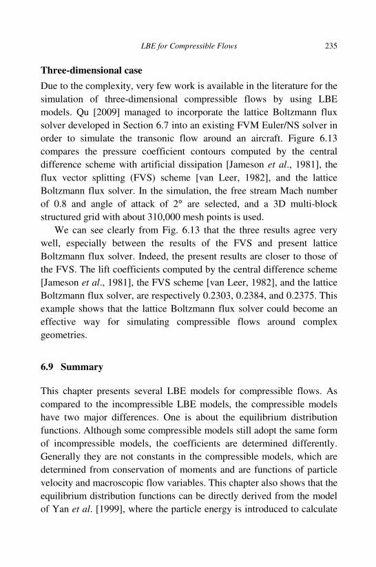
LBE for Compressible Flows 235
Three-dimensional case
Due to the complexity, very few work is available in the literature for the
simulation of three-dimensional compressible flows by using LBE
models. Qu [2009] managed to incorporate the lattice Boltzmann flux
solver developed in Section 6.7 into an existing FVM Euler/NS solver in
order to simulate the transonic flow around an aircraft. Figure 6.13
compares the pressure coefficient contours computed by the central
difference scheme with artificial dissipation [Jameson et al., 1981], the
flux vector splitting (FVS) scheme [van Leer, 1982], and the lattice
Boltzmann flux solver. In the simulation, the free stream Mach number
of 0.8 and angle of attack of 2° are selected, and a 3D multi-block
structured grid with about 310,000 mesh points is used.
We can see clearly from Fig. 6.13 that the three results agree very
well, especially between the results of the FVS and present lattice
Boltzmann flux solver. Indeed, the present results are closer to those of
the FVS. The lift coefficients computed by the central difference scheme
[Jameson et al., 1981], the FVS scheme [van Leer, 1982], and the lattice
Boltzmann flux solver, are respectively 0.2303, 0.2384, and 0.2375. This
example shows that the lattice Boltzmann flux solver could become an
effective way for simulating compressible flows around complex
geometries.
6.9 Summary
This chapter presents several LBE models for compressible flows. As
compared to the incompressible LBE models, the compressible models
have two major differences. One is about the equilibrium distribution
functions. Although some compressible models still adopt the same form
of incompressible models, the coefficients are determined differently.
Generally they are not constants in the compressible models, which are
determined from conservation of moments and are functions of particle
velocity and macroscopic flow variables. This chapter also shows that the
equilibrium distribution functions can be directly derived from the model
of Yan et al. [1999], where the particle energy is introduced to calculate
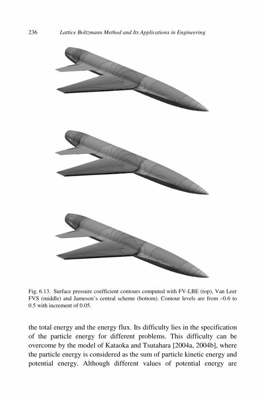
236 Lattice Boltzmann Method and Its Applications in Engineering
the total energy and the energy flux. Its difficulty lies in the specification
of the particle energy for different problems. This difficulty can be
overcome by the model of Kataoka and Tsutahara [2004a, 2004b], where
the particle energy is considered as the sum of particle kinetic energy and
potential energy. Although different values of potential energy are
Fig. 6.13. Surface pressure coefficient contours computed with FV-LBE (top), Van Leer
FVS (middle) and Jameson’s central scheme (bottom). Contour levels are from –0.6 to
0.5 with increment of 0.05.

LBE for Compressible Flows 237
assigned to different lattice directions, the model in fact only assigns the
potential energy to the static particle. In contrast, the model of Qu et al.
[2007a, 2007b], which is based on the circular function, takes the same
particle potential energy for different lattice directions. This is reasonable
as the potential energy reflects the contribution of kinetic energy from
the rotational velocity, which is independent of the translational velocity.
The particle potential energy of Qu et al. [2007a, 2007b] cannot be
chosen arbitrarily. It is calculated from the internal energy of the mean
flow. The adaptive model of Sun [2000b] is different from other
compressible models in the way that the particle mass, momentum and
energy are all transported along a streaming velocity, which is the sum of
the mean flow velocity and the lattice velocity. In general, the position
after the streaming is not on the mesh point. Thus, interpolation is
necessary. Another drawback of the adaptive model is that the relaxation
parameter τ is usually fixed as 1.
The compressible LBE models often encounter numerical instability
when the normal streaming-collision process is applied. To get a stable
solution, they are usually applied with the solution of discrete velocity
Boltzmann equation (DVBE). As upwind schemes are needed to solve
DVBE, the numerical stability of compressible models with solution of
DVBE is actually enhanced by artificial dissipation.
As compared to the incompressible models, the form of equilibrium
distribution functions is much more complicated for the compressible
models, especially for two- and three-dimensional cases. To overcome
this difficulty, this chapter presents a lattice Boltzmann flux solver,
which applies a one-dimensional LBE model to the local Riemann
problem at the cell interface. The flux evaluated by LBE at the cell
interface can be used in the solution of Euler equations by the finite
volume method. Numerical experiments showed that this solver can be
effectively applied to complicated two- and three-dimensional
compressible flows, indicating that this solver has a great potential for
real application.
In summary, the work for compressible flows is far behind that for
incompressible flows. More research efforts are needed to tackle the
challenging issues occurred in the application of LBE for compressible
flows.

This page intentionally left blankThis page intentionally left blank
239
Chapter 7
LBE for Multiphase and
Multi-component Flows
In the natural world and industrial processes, fluids usually contain
impurities more or less, and so most flows, strictly speaking, are
multiphase and/or multi-component ones. A multi-component system is a
mixture comprised of different fluid species, while a multiphase fluid
system involves obvious phase interfaces (e.g. gas-liquid mixture).
Furthermore, a multi-component fluid can be either miscible (e.g., air) or
immiscible (e.g., air-water), and a multiphase system can contain one or
more components.
The macroscopic dynamics of a multiphase or multi-component flow
is usually very complicated due to large scale disparities and the
coupling between mass transfer, phase segregations/separations, and
even chemical reactions. Traditional fluid dynamical models and
numerical methods may encounter difficulties for these systems. For
example, an equation of state is required in order to model two-phase
flows, which is usually difficult to obtain in the interfacial region. On the
other hand, it is well understood that the macroscopic behaviors of
multiphase and multi-component flows are the natural consequences of
microscopic interactions among fluid molecules. Therefore, in principle,
multiphase flows can be simulated by numerical methods based on
realistic microscopic physics such as molecular dynamics (MD).
However, such methods are usually very computational expensive and
consequently become impractical for simulating macroscopic flows. In
recent years, there is a trend to construct numerical methods for such
flows based on mesoscopic theories that connect the microscopic and
macroscopic descriptions of the dynamics, among which the LBE has
received particular attentions. Thanks to the kinetic nature of the LBE,

240 Lattice Boltzmann Method and Its Applications in Engineering
inter-molecular interactions can be incorporated into a LBE model in a
straightforward way so that it can be used to simulate a multiphase or
multi-component system effectively. This feature is also recognized as
one of the main advantages of LBE that distinguishes it from other
numerical methods.
A variety of LBE models for multiphase and multi-component flows
have been established from different viewpoints, and in this chapter
several typical kinds of such models will be presented.
7.1 Color Models
7.1.1 LBE model for immiscible fluids
The first LBE model for multiphase flows is put forward by Gunstensen
et al. [1991], which is an improved version of the multiphase LGA
model of Rothman and Keller [1988]. In this model, phases are denoted
by different colors, and inter-particle interactions, which are responsible
for phase separations and segregations, are modeled by local color
gradients associated with density differences between two phases.
Taking a two-phase system as an example, the color-gradient model
uses two types of distribution functions, fri and fbi , to represent the red
and blue fluids, respectively. The total distribution function for the
mixture, fi = fri + fbi , evolves as [Alexander et al., 1993; Gunstensen
et al., 1991]
( , ) ( , ) pci i t t i i if t f tδ δ+ + − = Ω + Ωx c x , (7.1)
where ciΩ denotes the collision effects and p
iΩ means the perturbation
aroused by interfacial tensions. The densities and velocities for each fluid
and the mixture are defined as
, ,
.
, ,
,
kk ki k i ki
i i
r b r r b b
f f k r bρ ρ
ρ ρ ρ ρ ρ ρ
= = =
= + = +
∑ ∑u
u u u
c (7.2)
In the model of Gunstensen et al., the collision term is constructed
from the MZ collision model [McNamara and Zanetti 1988], which
originates from LGA collision rules. As mentioned in Chapter 1, such a

LBE for Multiphase and Multi-component Flows 241
model may encounter some numerical instabilities and the computational
efficiency is not satisfactory, either. Later Alexander et al. [1993] proposed
a BGK model for ciΩ . In order to determine p
iΩ , an order parameter is
introduced first to describe the phase difference,
( , ) ( , ) ( , )r bt t tψ ρ ρ= −x x x . (7.3)
A local color gradient is then defined as
( , ) ( , )i i t
i
t t+= ∑x c xG c δψ , (7.4)
from which piΩ is defined,
| |cos(2 )pi iA=Ω θG , (7.5)
where θi is the angle between ci and G, A is a parameter that controls the
surface tension σ, i.e., σ ∼ Aρλ, where λ is the eigenvalue of the collision
operator ciΩ related to the viscosity. Obviously, the color gradient is 0 in
bulk regions, and so is piΩ . In other words, surface tension only takes
effects in the interfacial region, which is physically sound.
After obtaining piΩ and c
iΩ , the total distribution function can be
calculated according to Eq. (7.1), and the red and blue distribution
functions are then obtained by a re-coloring step, which solves the
following maximum value problem
,
( , ) max ( )ri bi
ri bi ri bi if f
i
W f f f f′′ ′′
′′ ′′ ′′ ′′ = −
∑ c , (7.6)
subjected to the following constraints,
,r ri r ri bi i
i
f f f fρ ρ′′ ′′ ′′ ′′= = + =∑ , (7.7)
where kif ′′ is the distribution function after the re-coloring, ρr and fi are
the density and distribution function before the collision step. The
essence of this re-coloring step is to enforce the direction of the color
flux H ≡ ρrur − ρbub to match that of the color gradient G. During this
process, the fluid is driven to the bulk region with the same color, and
phase separation is then induced.

242 Lattice Boltzmann Method and Its Applications in Engineering
In summary, the color-gradient model of Gunstensen et al. can be
realized by the following four steps:
• Collision: cii iff =′ + Ω ;
• Perturbation: pi i if f′′ ′= + Ω ;
• Re-coloring: Compute rif ′′ and bif ′′ from Eq. (7.6);
• Streaming: ( , ) ( , )ri i t t rif t f tδ δ ′′+ + =x c x , ( , ) ( , )bi i t t bif t f tδ δ ′′+ + =x c x .
In the original model, the collision process is made for the total
distribution function of the mixture. Grunau et al. [1993] presented a
slightly modified color-gradient model in which collisions are also
carried out for the distribution functions of different fluids,
( , ) ( , ) pri i t t ri ri rif t f tδ δ+ + − = Ω + Ωx c x , (7.8)
( , ) ( , ) pbi i t t bi bi bif t f tδ δ+ + − = Ω + Ωx c x , (7.9)
where riΩ and biΩ
are the collision operators for the red and blue fluids,
respectively,
( )1, ,eq
ki ki ki
k
f f k r bτ
Ω = − − = . (7.10)
Here the equilibrium distribution function depends on the density ρk and
the mixture velocity u. As an example, the equilibrium distribution
function of the D2Q7 model is defined by
2
( )
22
, 0,6
1 1 2( )
, 0,6 3 3 3
kk
eq kki
k i i
k
mu i
mf
ui
m
− = + = + + − ≠ + ⋅ ⋅
c u c u
ρ
ρ
(7.11)
where k = r, b and mk denotes the ensemble average value of the static
particles of phase k. When the velocity is zero, in order to obtain a stable
phase interface, it requires
6 6
r b
r b
dm m
= =+ +ρ ρ
. (7.12)
The additional terms pkiΩ in Eqs. (7.8) and (7.9) represent the
perturbations caused by the surface tension,
02| |
2
k ipki
A
Gθ
Ω = −
⋅
GcG , (7.13)
LBE for Multiphase and Multi-component Flows 243
with Ak being a parameter related to surface tension and θ0 a model-
dependent constant. For example, θ0 = 1/2 for the D2Q7-FHP model.
The model of Grunau et al. also needs the re-coloring processes.
Specifically, the direction of the momentum of the red fluid is enforced
to match that of the color gradient by maximizing the function
( )r r ⋅− u Gρ , which can give the new value of fri ; then the distribution
function of the blue fluid is calculated as fbi = fi − fri . Theoretical analysis
shows that the surface tension in the color model of Grunau is related to
Ar and Ab . Particularly, when Ar = Ab = A, the coefficient of surface
tension in the D2Q7 model is
9 (12 )r bA d m mσ τ= + + , (7.14)
where 2 /( )r b r b= +τ τ τ τ τ is the average relaxation time at the phase
interface.
In the above color-gradient models, the solution of the maximum
value problem in the re-coloring process is usually computational
expensive. Some simplified versions have been developed later. For
example, d’Ortona et al. [1995] proposed an alternative re-coloring
method based on Gunstensen’s model,
2
cosr r bri i if f
ρ ρ ρβ θ
ρ ρ′′ ′′= + ,
2cosb r b
bi i if fρ ρ ρ
β θρ ρ
′′ ′′= − , (7.15)
where the parameter 0 ≤ β ≤ 1 is related to the interface width: a larger
value of β will give a thinner interface. Specifically, the above color
model can be applied to miscible fluids as A = β = 0. Further
improvements in color models can also be found in [Tölke et al., 2002].
7.1.2 LBE model for miscible fluids
Although the color-gradient models can be used to simulate miscible
fluids by adjusting the model parameters, the main aim of these models
is to capture the interfacial dynamics in multiphase systems. Flekkøy
[1993] established an alternative kind of color model for miscible fluids
directly. Instead of describing the distribution function of each fluid, this
model adopts the sum and difference of the distribution functions as the

244 Lattice Boltzmann Method and Its Applications in Engineering
new basic variables,
,i ri bi i ri bif f f g f f= + = − . (7.16)
The corresponding evolution equations are
( )1( , ) ( , ) eqi i t t i i if t f t f f
ν
δ δτ + + − = − − x c x , (7.17)
( )1( , ) ( , ) eqi i t t i i i
d
g t g t g gδ δτ + + − = − − x c x , (7.18)
where τv and τd are the corresponding dimensionless relaxation times,
and ( )eqif has the same form as that of the standard DnQb-LBGK model,
while
( )
21eq i
i i
s
gc
ω ϕ = +
⋅
c u
, (7.19)
where r b ii g= − = ∑ϕ ρ ρ is the density difference, and ii f= ∑ρ and
i ii f= ∑u cρ are the density and momentum of the mixture.
The evolution equation of fi is the same as that in single component
LBE models. As a result, the corresponding hydrodynamic equations of
the mixture are also the Navier-Stokes equations. On the other hand, the
Chapman-Enskog analysis of Eq. (7.18) gives the following convection-
diffusion equation,
2 2
2( )
s
DD
t c
ϕϕ ϕ ϕ
∂+ ⋅ ∇ = ∇ − ⋅ ∇
∂u u , (7.20)
where the diffusion coefficient D is
2 1
2s d tD c τ δ = −
. (7.21)
Dimensional analysis shows that the ratio of the second term over the
first one on the right hand side of Eq. (7.20) is in the order of
2 2 20 2
2
/
1/
su c LM
L= , (7.22)

LBE for Multiphase and Multi-component Flows 245
where u0 and L0 are the characteristic velocity and length, respectively.
This result indicates that for flows with a small Mach number, the second
term can be neglected and thus Eq. (7.20) becomes a standard
convection-diffusion equation. As a result, this LBE model can capture
the hydrodynamics and diffusion process of a miscible fluid.
Remark: The color models are the earlier LBE methods for
multiphase/multi-component systems. These models have been
successfully applied to complex interfacial flows such as multiphase
flows in porous media [Tölke et al., 2002] and the spinodal
decomposition [Alexander et al., 1993]. However, LBE models of this
type also suffer from several limitations, such as the anisotropy of
surface tension, the spurious currents in the vicinity of interfaces, and
the difficulty to include thermodynamics.
7.2 Pseudo-Potential Models
7.2.1 Shan-Chen model
The key point of the color models is to redistribute the fluid particles
based on the color gradient. Actually, the interaction force in such
models comes from the difference between the averaged molecular
forces on the two sides of the interface. Shan and Chen [1993] presented
a LBE model (referred to SC model) which could depict the interaction
between fluid particles more accurately and straightforwardly by
introducing a pseudo potential.
For a fluid composed of S components, the SC LBE model can be
written as
( )1( , ) ( , ) eq
ki i t t ki ki ki
k
f t f t f fδ δτ
+ + − = − − x c x , 1k S= ∼ , (7.23)
where ( ) ( )( , ) eq eqi kki kf E ρ= u
is the equilibrium distribution function of the
k-th component, k kii f= ∑ρ is the density of the k-th component, and ( )eqku is the equilibrium velocity to be determined. The formulation of Ei
depends on the choice of the lattice model. For the FHP or FCHC lattice,
( ) ( )( ) 2( ), , 0,eq
i k ke
kq
kE d u i = − = uρ ρ

246 Lattice Boltzmann Method and Its Applications in Engineering
( )
( )( )
(( )
2
(
)
( )2
)
( )1,
( 2), 0,
2 2
eqk i kk
i k k
eqi
q
k eqk
ek
k
DdE
b b
D D Du i
b b
−= +
+
⋅
+ − ≠⋅
c uu
c u
ρρ ρ
ρρ
(7.24)
where <1kd is a constant. The SC model employs a non-local interaction
which comes from a potential,
x x x x x x( , ) (| |) ( ) ( )kk kk k kV G ψ ψ= −′ ′ ′ , (7.25)
where kkG is a Green function which controls the interaction intensity
between component k and k ; kψ denotes an effective density of the
component k and is usually a function of ρk . Generally, the SC model
considers only the nearest neighbour interactions, and the function
kkG can be modelled as
x x
x xx x
,0, | |(| |
.)
, | |
x
kk
kk x
Gδ
δ
− >− = − =
′′
′G
(7.26)
In the above model, the modulus of kkG decides the interaction
intensity between component k and k . The sign of kkG determines whether
the interaction force is attractive (negative) or repulsive (positive).
The kkG forms a symmetric S × S interaction matrix G. According to
this pseudo potential, the total force acting on the k-th fluid can be
expressed as
x x x c cF ( ) ( ) ( )k k kk k i t i
k i
ψ ψ δ= − +∑ ∑G . (7.27)
Obviously, when δx → 0, ( , )k kkkV′= −∇ ′∑x x xF . As mentioned in
Chapter 3, there are several approaches to include the interaction force
into LBE. In the original SC model, this is achieved through the
equilibrium velocity u( )eqi ,
F
u x xu( )( ) ( )eq k
k tk
k
τ δρ
= + , (7.28)
where u is the velocity of the mixture defined by
cu uk k i ki
k k i
fρ ρ= =∑ ∑∑ , (7.29)

LBE for Multiphase and Multi-component Flows 247
where kk= ∑ρ ρ is the density of the mixture. This approach will
introduce some discrete lattice errors as described in Chapter 3. After
neglecting such errors, the macroscopic equations derived from the SC
model for a single component system (i.e. S = 1) can be expressed as
( )u 0t
ρρ
∂+ ∇ ⋅ =
∂, (7.30)
( )
( )u
uu pt
ρρ
∂+ ∇ ⋅ = −∇ + ∇ ⋅
∂τ , (7.31)
where τ is the viscous stress, the same as the standard LBGK models;
the pressure p now depends on the interaction force,
0 2(1 )
( )2
d bp
D Dρ ψ ρ
−= + G , (7.32)
where 11=G G is the internal interaction among the fluid. Obviously the
equation of state is one for non-ideal gases. When the potential V is
properly chosen so that p is a non-monotonic increasing function of the
density ρ, phase separation can appear. For the potential with the form
(7.25), phase separation can be initiated by choosing a strong G
with a nonlinear potential function ψ . Shan and Chen suggested using
the following effective density function,
0/0 1 k k
k k e ρ ρψ ρ − = − , (7.33)
where ρk0 is a reference density of the k-th component. On the other hand,
Qian et al. [1995] proposed a fractional form for the density function.
7.2.2 Shan-Doolen model
Soon after the Shan-Chen model, Shan and Doolen [1995] developed an
improved version (denoted by SD model) to reduce some of the artifacts.
First, the definition of the equilibrium velocity ( )u
eq
k is changed to
F
u u( )eq
k tk
k
τ δρ
+′= , (7.34)

248 Lattice Boltzmann Method and Its Applications in Engineering
where ′u is required to satisfy momentum conservation in the case of no
forces, i.e.,
uc ( )( , ) 0eqi
ki kki
k i k
f f ρτ
′− = ∑∑ , (7.35)
which gives that
u
u /k k k
k kk k
ρ ρ
τ τ′ = ∑ ∑ . (7.36)
In the presence of the interaction force, particle collisions do not
conserve the momentum locally. But the overall momentum of the
system is conserved as the interaction matrix G is symmetric. In the SD
model, the velocity of the fluid is redefined by the average of pre-
and post-collision momenta, /2k t kkkk= +∑ ∑u u Fρ ρ δ , which can reduce
the discrete errors significantly.
The Chapman-Enskog analysis shows that the SD model leads to the
following continuity equation for each species,
u j( )kk k
t
ρρ
∂+ ∇ ⋅ = −∇ ⋅
∂, (7.37)
where j u u( )k k kρ= − is the diffusive mass flux of the k-th component,
which is related to the pressure, interaction force, and species
concentrations. For the FHP and FCHC models, it can be shown that
(1 )1
21
( 1 / 2) (1 ) ,
kkk k k k k
t
k k k k k k k k
k k k
dx p
D
x p x dD
− = − + − ∇ − ∇ + + + ∇ − − ∇ ∑ ∑ ∑F
jFτ τ ρ
δ
τ τ τ ρ
(7.38)
where xk = ρk/ρ is the mass fraction of the k-th species. The pressure is
similar to that of the SC model,
,
1(1 )
2k k kk k k
k k k
bp d
Dψ ψρ
= − + ∑ ∑G . (7.39)
It is noteworthy that when 0kk =G , the pressure should obey an equation
of state of ideal gases, i.e. kkp p= ∑ . This leads to 21 /k s kd Dc m− = ,
where cs is the sound speed in the fluid mixture, and mk
is the molecular
mass of the k-th component.

LBE for Multiphase and Multi-component Flows 249
The mass diffusive flux jk can be decomposed into two parts, ( ) ( )x p
k k k= +j j j , where
( )
1 1 1
( ) /S S S
xkm n kn m n n n mk
m n n
bA A x A x x
D = = =
= − ∇ ∑ ∑ ∑jρ
α α , (7.40)
( )
1 1
/S S
pkm m m mk
m m
x A x p= =
= ∇ ∑ ∑j α , (7.41)
where the coefficients are given by
1
1 1
1( 0.5)( )
( ) ,
Sm
km m k km k k n n t
n
S Sm
n k kn k k n n nm n t
n n m
dx x x
b
x x x
=
= =
− = − − + − − + −
+
∂∂
∑
∑ ∑
α τ δ τ τ δ
τ δρ
ψψδ τ τ ζ
(7.42)
1
1 Sm m
m mn m
nm
dA
b =
∂∂
−= + ∑ ζ ψ
ρ
ψ. (7.43)
The coefficient before the concentration gradient in Eq. (7.40) is just the
mutual diffusivity.
It can be proved that 0kk =∑ j . Then the mass conservation equation
of the mixture can be obtained by summing up Eq. (7.37) over k ,
u( ) 0t
ρρ
∂+ ∇ ⋅ =
∂. (7.44)
The momentum equation can also be derived based on the Chapman-
Enskog expansion, which is similar to that of the SC model except with a
viscosity defined by
1 1
2 2 k k
k
xD
ν τ = − + ∑ . (7.45)
7.2.3 Numerical schemes for interaction force
In either the SC model or the SD model, spurious velocities often appear
in the vicinity of a phase interface [Hou et al., 1997]. Recently, Shan
[2006] found that the isotropy of the force discretization schemes has
significant influences on the spurious velocities, and the use of

250 Lattice Boltzmann Method and Its Applications in Engineering
high-order isotropic schemes can reduce the magnitudes of spurious
velocity greatly.
Consider a single component fluid with long distance interactions. In
this system the force on a particle located at x exerted by a particle
located at x′ can be written as
x x x x x x x x( , ) (| |) ( ) ( ) ) (G ψ ψ′ ′ ′ ′= − − −F . (7.46)
Then the total force experienced by the fluid particle can be expressed as
F x x x x x x x x( ) ( ) (| |) ( )( )G dψ ψ′ ′ ′ ′= − − −∫ . (7.47)
Assuming that x x(| | )G ′ − is isotropic, the above integral can be
evaluated by the discrete values at the neighboring nodes,
F x x x c c2
1
( ) ( ) ( ) ( )N
i i i
i
w cψ ψ=
= − +∑G , (7.48)
where : 1,2, , i i N+ =x c are N nodes surrounding x, 2( )iw c is the
weight coefficient of the integral. Take Taylor expansion of x c( )iψ + ,
F(x) can be approximated as
( ) ( 1)
0
1( ) ( ) [ ( )] :
!n n
n nζψ ψ
∞+
=
= − ∇∑F x xx E , (7.49)
where
( ) 2
1
( )N
ni i i i
i n
w c=
= ∑ cE c c
. (7.50)
The symmetric properties of the lattice lead to
E( )( )
0, 1, 3, 5,
0, , ,, 2 4n
n nn x
n
e nδ
== ∆ =
(7.51)
where en is a constant and ( )n∆ is an n-th order symmetric tensor.
Since the interaction force F(x) is isotropic, Eq. (7.49) holds only
when all the E(n) are so. But due to the finiteness of the discrete velocity
set, this condition cannot be fulfilled. However, E(n) can achieve
high-order isotropy by properly choosing the weight coefficients 2( )iw c .
Table 7.1 gives several isotropic tensors E(n) and the corresponding
weights for two- and three-dimensional lattices. Numerical results of a

LBE for Multiphase and Multi-component Flows 251
static droplet show that high-order isotropic schemes can decrease the
spurious velocity greatly [Shan, 2006].
Remark: In pseudo-potential LBE models, the microscopic interactions,
which reflect the physical nature of the multiphase/multi-component
flows, are modelled directly. Due to this clear picture and the simplicity,
such models are widely used in many fields. However, theoretical
analysis shows that the pseudo-potential models are consistent with
thermodynamic theories only when the effective density function takes a
special exponent form [Shan and Chen, 1994].
7.3 Free Energy Models
The color and pseudo-potential LBE models are both phenomenological
models. Swift et al. [1995, 1996] developed an alternative type of LBE
models for multiphase/multi-component systems based on free energy
theory. The basic idea is to devise a suitable equilibrium distribution
function based on some free energy functions, in which the
thermodynamic pressure tensor is incorporated.
7.3.1 Models for single component non-ideal fluid flows
For a one-component non-ideal fluid, the van der Waals theory shows
that the free energy of the system can be expressed as
( ( ), ( )) ( ( ))T W dΨ ψ ρ ρ = + ∇ ∫ x x x x , (7.52)
Table 7.1. Weight coefficients and isotropic E(n) (Shan, Phys. Rev. E 73, 047701 2006).
( )nE 2 2/i xe δ
n 1 2 3 4 5 6 8
4 1/3 1/12
2D 6 w 4/15 1/10 1/120
8 4/21 4/45 1/60 2/315 1/5040
4 1/6 1/12
3D 6 w 2/15 1/15 1/60 1/120
8 4/45 1/21 2/105 5/504 1/315 1/630 1/5040

252 Lattice Boltzmann Method and Its Applications in Engineering
where ( )ψ ρ is the free energy density in the bulk phase, and ( )W ρ∇
is
the free energy related to surface tension. One common free energy
formulation is
2| |2
W = ∇κρ , (7.53)
where the parameter κ is related to the surface tension. For example, for
a flat interface located at z = 0, the surface tension is defined as
2
zdz
ρσ κ
∂
∂
= ∫ . (7.54)
According to the free energy Ψ, a non-local pressure can be defined as
2 20( ) | |
2p p
δΨ κρ Ψ κρ ρ ρδρ
= − = − ∇ − ∇x , (7.55)
where 0 ( ) ( )p ρψ ρ ψ ρ′= − is the equation of state. Then the thermo-
dynamic pressure tensor, which considers the contribution of the
interface, can be written as
P px x
αβ αβ
α β
ρ ρδ κ
∂ ∂′ = +∂ ∂
. (7.56)
Note that P′ is different from the pressure tensor f τ′≡ = +∫P CC P
in kinetic theory.
In order to obtain a LBE model which is consistent with the
above thermodynamical theory, Swift et al. suggested using an
equilibrium distribution function with the density gradient in the LBGK
model,
( )( )1( , ) ( , ) , ,eq
i i t t i i if t f t f fδ δτ
ρ ρ + + − = − − ∇ c ux x , (7.57)
where ( )eqif are constructed to enforce the following constraints,
( ) ( ) ( ), ,eq eq eqi i i i i i
i i i
f f f ′= = = +∑ ∑ ∑c cu P uuρ ρ ρc . (7.58)

LBE for Multiphase and Multi-component Flows 253
Similar to the standard LBGK model, the equilibrium distribution
function ( )eqif
is also a polynomial of the fluid velocity u. For example, in
the FHP model ( )eqif
can be expressed as
( ) 2 2( ) ( ) : , 0eqi i i i if A B Cu D G i= + + + +⋅ ≠⋅c cu ccu , (7.59)
( ) 20 0 0eqf A C u= + . (7.60)
According to the conditions given by Eq. (7.58), the coefficients in ( )eqif
can be obtained as
0 06 ,A A Cρ ρ= − = − , (7.61)
20
1 2( ), , ,
3 3 6 3A p B C D
ρ ρ ρκρ ρ= − ∇ = = − = , (7.62)
2 22
,3 3
xx yy xyG G Gx y x y
κ ρ ρ κ ρ ρ ∂ ∂ ∂ ∂ = − = − = ∂ ∂ ∂ ∂ . (7.63)
Equation (7.58) also indicates that the collision operator of the free-
energy model conserves both mass and momentum locally.
With the above equilibrium distribution function, together with the
definition of fluid velocity as i ii f= ∑u cρ , the hydrodynamic equations
recovered from the free-energy model are
( ) 0t
ρρ
∂+ ∇ ⋅ =
∂u , (7.64)
20
0
( )( [ ( )]
1[ ( ) ],
2
) ( )
t
pt
p
∂+ ∇ ⋅ = −∇ + ∇ + ∇ ∇ ⋅
∂ ∂− − ∇ ⋅ ∇ + ∇ ∂
uuu u u
u u
ρρ ν ρ λ ρ
τ δ ρ ρρ
(7.65)
where
01 1 1 1,
4 2 2 2t t
pν τ δ λ τ δ
ρ
∂ = − = − − ∂. (7.66)
The last term on the right hand side of the momentum equation is zero in
the bulk phase, where the equations reduce to the standard Navier-Stokes
equations. But in the vicinity of phase interface where density gradient is
large, this term should be considered.

254 Lattice Boltzmann Method and Its Applications in Engineering
7.3.2 Model for binary fluid flows
Free-energy LBE model for non-ideal fluid flows with two components
was also developed [Swift et al., 1996]. This model uses two distribution
functions to simulate the overall system, which is similar to the miscible
model presented by Flekkøy [1993] as described in subsection 7.1.2.
The difference between these two models lies in the equilibrium
distribution functions ( )eqif and ( )eq
ig : the free-energy model considers the
in-homogeneity of the fluid. Specifically, ( )eqif still satisfies the
constraints given by Eq. (7.58), except that the density ρ and velocity u
are for the mixture; on the other hand, ( )eqig now are enforced to satisfy
the following constraints,
u I uc c uc( ) ( ) ( ), ,eq eq eqi i i i i i
i i i
g g gϕ ϕ µ ϕ= = = Γ∆ +∑ ∑ ∑ , (7.67)
where µ∆ is the chemical potential difference between the two
components, and Γ is the mobility. Here the thermodynamic pressure
tensor P′ and the chemical potential difference µ∆ can be obtained
according to certain free energy models for two-phase systems. Swift
et al. [1996] considered the following free energy,
2 2
2 2( , , ) | | | |T d = + ∇ + ∇ ∫ xκ κΨ ψ ρ ϕ ρ ϕ , (7.68)
where the bulk free-energy density is given by
2
21 ( )ln
4 2 2
( ) ln ,2 2
G RTRT
RT
ϕ ρ ϕψ ρ ρ ρ ϕ
ρ
ρ ϕρ ϕ
+ = − − + + − + −
(7.69)
where G denotes the interaction strength. As RT < G/2, phase separation
will occur. Furthermore, from this free-energy, one can derive the
chemical potential difference and the thermodynamic pressure tensor,
21 /
ln2 2 1 /
G RT + ∆ = − + − ∇ − ϕ ρϕ
µ κ ϕρ ϕ ρ
, (7.70)
P px x x x
β αβ
β
α
βα α
ρ ρ ϕ ϕδ κ κ
∂ ∂ ∂ ∂′ = + +∂ ∂ ∂ ∂
, (7.71)

LBE for Multiphase and Multi-component Flows 255
where
( )2 2 2 2( ) | | | |2
p RT= − ∇ + ∇ − ∇ +∇κ
ρ κ ρ ρ ϕ ϕ ρ ϕ . (7.72)
With these expressions, the coefficients in ( )eqif
can be written as
0 06 ,A A Cρ ρ= − = − , (7.73)
2 20
1 2( ), , ,
3 3 6 3A p B C D
ρ ρ ρκρ ρ κϕ ϕ= − ∇ − ∇ = = − = , (7.74)
2 2 2 2
3xx yyG G
x y x y
κ ρ ρ ϕ ϕ ∂ ∂ ∂ ∂ = − = − + − ∂ ∂ ∂ ∂ , (7.75)
2
3xyG
x y x y
κ ρ ρ ϕ ϕ ∂ ∂ ∂ ∂ = + ∂ ∂ ∂ ∂
. (7.76)
Similarly, ( )eqig
reads
c u uc( ) 2 2( ) ( ) , 0 eqi i ig H K Ju Q i⋅+ + + ⋅= ≠ , (7.77)
( ) 20 0 0eqg H J u= + , (7.78)
where
0 06 ,H H Jϕ ϕ= − = − , (7.79)
1 2
, , ,3 3 6 3
H K J Qϕ ϕ ϕ
µ= Γ∆ = = − = . (7.80)
With the above expressions, the recovered hydrodynamic equations of
the FHP free-energy model read
u( ) 0t
ρρ
∂+ ∇ ⋅ =
∂, (7.81)
u P2( )t
ϕ ϕϕ θ ϕ θ
ρ
∂ ′+ ∇ ⋅ = Γ ∇ − ∇ ⋅ ∇ ⋅ ∂
, (7.82)
u
uu u u20
( )( )( ) [ ( )]p
t
ρρ ν ρ λ ρ
∂+ ∇ ⋅ = −∇ + ∇ + ∇ ∇ ⋅
∂, (7.83)

256 Lattice Boltzmann Method and Its Applications in Engineering
where ν and λ is given by Eq. (7.66). The transport coefficient in
Eq. (7.82) is
1
2d tθ τ δ
= − , (7.84)
where τd is the relaxation time in the evolution equation of gi .
7.3.3 Galilean invariance of the free-energy LBE models
Although the free-energy LBE model is constructed from thermo-
dynamic theories, it still has some undesirable features, one of which is
the violation of the Galilean invariance. In the recovered momentum
equation, the density in the viscous stress appears in the first order
derivative, i.e.
u u2( ) [ ( )]ν ρ λ ρ= ∇ + ∇ ∇ ⋅τ . (7.85)
In bulk region the density is nearly constant and Eq. (7.85) is Galilean
invariant approximately. However, in the vicinity of an interface where
the density gradient is large, the Galilean invariance of Eq. (7.85) will be
broken and nonphysical phenomenon will appear. Actually, it has been
reported that a droplet with an initial sphere shape will become an elliptic
one in a uniform flow field [Inamuro et al., 2000; Kalarakis et al., 2002].
The lack of Galilean invariance of the free-energy model was first
found by Swift et al. [1996]. They proposed a method to remedy this
problem, which enforces the second-order moment of the equilibrium
distribution function to satisfy the following condition,
( )1 2( )eq
i i i
i
c c f u u P u u uα β α β αβ α β β α γ γρ ω ρ ρ ω ρ′= + + ∂ + ∂ + ∂∑ , (7.86)
where ω1 and ω2 are two parameters that can be adjusted to recover the
Galilean invariance partially. For the aforementioned FHP model, the
Chapman-Enskog analysis shows that the viscous stress is now,
( ) ( ) 1
2 1
( )
( ) (2 ) .
u u u
u u
αβ α α β β α α α β α
β α α α α β
ν ρ λρ λ ν ω ρ
λ ω ρ ν λ
τ
ω ρ
= ∂ ∂ + ∂ ∂ + ∂ − − ∂
+ ∂ − ∂ − ∂ − + ∂
(7.87)
In order to recover the Galilean invariance, the last three terms in
Eq. (7.87) should vanish. However, since the viscosity ν is always
positive, these three non-Galilean invariant terms cannot be completely

LBE for Multiphase and Multi-component Flows 257
removed by choosing ω1 and ω2 . On the other hand, by choosing
ω1 = λ − 2ν and ω1 = λ, we can eliminate the last two terms so that the
Galilean invariance is partially recovered.
Inamuro et al. [2000] built another D2Q9 free-energy model with
improved Galilean invariant properties. The equilibrium distribution
function of this model is
( ) 20
2 2
2 4 2
3 2
( ), 0,
2 2
:eqi i i i i
iii
s s s
f p
ui
c c c
= − ∇ + ⋅ ∇ + + + − ≠
⋅
⋅
u G c c
uu cc
ω κρ ρ ω ρ ω
ω ρ
(7.88)
2
( ) 20 0 0 2
52
3 2
eq
s
uf p
c = − − ∇ + ⋅ ∇ − uρ κρ ρ ω ρ ω ρ , (7.89)
where 2 1/3sc = , ωi is the weight coefficient which is the same as that in
the standard D2Q9 model, ω is an adjustable coefficient aiming at
eliminating the Galilean variance. The second-order tensor G in
Eq. (7.88) is defined by
.
9
2
92
4
G u ux x x x
ux x x
αβ α β
α β β α
γ αβ
γ γ γ
ρ ρ ρ ρκ ω
ρ ρ ρκ ω δ
∂ ∂ ∂ ∂ = + + ∂ ∂ ∂ ∂ ∂ ∂ ∂ − + ∂ ∂ ∂
(7.90)
Asymptotic analysis shows that the parameter ω should be chosen as 2( 0.5)s tcω ν τ δ= = −
in order to recover the Galilean invariance.
Based on the FHP model developed by Swift et al., Kalarakis et al.
[2002] developed another free-energy model satisfying the Galilean
invariance by modifying the equilibrium distribution function. The basic
idea is to absorb the non-Galilean terms into the pressure tensor. The
correction method is similar to that by Swift et al., i.e. introducing two
adjustable terms into the thermodynamical pressure tensor P ′ as given
by Eq. (7.86). The two free parameters are chosen as
1 2 1 4p
ω ω νρ
∂ = = − ∂. (7.91)
Obviously, this correction method is identical to that of Inamuro if
/p∂ ∂ρ is neglected.

258 Lattice Boltzmann Method and Its Applications in Engineering
Recently, Zheng et al. [2005, 2006] presented an improved free-
energy LBM, in which the D2Q5 lattice velocity model is used to capture
the interface for the 2D case. It can recover the macroscopic Cahn-
Hilliard equation with the second order of accuracy. All of the above
improved free-energy models are shown to be able to reduce the non-
Galilean invariant effects. Numerical results demonstrated that the shape
of a single droplet or bubble in a uniform flow could be maintained. On
the other hand, it seems that the free-energy models for multiphase and
multi-component flows have some intrinsic limitations which require
further investigations.
Remark: The main difference between the free-energy models and the
pseudo-potential models lies in the force treatments: in the pseudo-
potential models, the effects of the interaction force are reflected in the
first-order moment of the equilibrium distribution function, while in the
free-energy models the effects are reflected in the second-order moment
of the equilibrium distribution function. From the microscopic point of
view, the inter-particle interactions should influence the momentums of
the flow (i.e., the first-order velocity moment). But at mesoscopic scale,
the overall effects from the microscopic interactions can be reflected in
the thermodynamic pressure tensor. Therefore, as a mesoscopic method,
the free-energy LBE model is also an effective approach.
7.4 LBE Models Based on Kinetic Theories
As shown in Chapter 1, the LBE for simple fluids can be derived from
the Boltzmann equation. Similarly, it is also possible to construct LBE
models for multiphase/multi-component flows based on corresponding
kinetic theories. An advantage of the LBE models obtained in this way is
that they will have a solid physical foundation. Recently, some of such
models have been developed successfully following this approach.
7.4.1 Models for single-component multiphase flows
Kinetic model for dense gases
The evolution of the single-particle distribution function of a dilute gas
can be well described by the Boltzmann equation. In a dilute gas, the

LBE for Multiphase and Multi-component Flows 259
mean free path is fairly larger than the molecular diameter. As a result,
the singlet distribution function can be treated to be independent from
others, and the molecular volume can be ignored during the collision
process. However, for a dense gas these assumptions do not hold
anymore, and the Boltzmann equation will fail to work. In such cases,
the Enskog equation [Chapman and Cowling, 1990] should be used
instead, which can be expressed as
a E
ff f
t
∂+ ⋅ ∇ + ⋅ ∇ = Ω
∂ξξ , (7.92)
where a is the acceleration due to an external force, ΩE is the Enskog
collision operator,
12
1 12
( ) ( ) ( , ) ( , )
( ) ( , ) ( , ) ( ,| |) .
E f f f
f f B d d d
ξ ξ
ξ ξ ξ
′ ′Ω = + +
− − −
∫ x k x x k
x k x x k V
σ
σ
χ σ
χ σ θ θ ε
(7.93)
Here σ is the diameter of the molecule, k is the unit vector directed from
the molecule with velocity ξ1 to that with velocity ξ along the line of
centers of the two colliding molecules. ξ
and ξ′
are the molecular
velocities before and after the collision, χ is the radial distribution
function (RDF) of two molecules at contact, which is evaluated at
location /2+x kσ . It depends only on the distance between the molecules
and is independent of its velocity. Actually, the function χ reflects the
increase in the collision probability in a dense gas. Usually, it is a
monotonic increasing function of the number density n or the parameter 3 32 /3 (2 /3 )b n m≡ =ρ πσ πσ ρ . It is clear that bρ is just one half of the
total volume of the gas molecules in a unit volume, 34 /3V n=σ πσ . As
such, 0 0.5bρ≤ ≤ . Generally χ is inversely proportional to (1 2 )lbρ− for
hard sphere gases (here l is a positive integer). For instance, the
Carnahan-Starling model [Carnahan and Starling, 1969] gives
3
1
(1 2 )
b
b
ρχ
ρ
−=
−. (7.94)
For a dilute gas χ = 1 as bρ → 0, and χ increases gradually as the gas
becomes denser. Particularly, when the gas is so dense that the molecules
cannot move, we have bρ → 0.5 and χ = ∞.
260 Lattice Boltzmann Method and Its Applications in Engineering
The Enskog collision operator ΩE reflects the finite volume effect in
dense gases, and it is a nonlocal operator. The collisions between the
finite-size molecules will induce momentum and energy transfer
(collisional transfer), which is not considered in the Boltzmann equation.
The Chapman-Enskog analysis of the Enskog equation leads to the
following hydrodynamic equations
u( ) 0t
ρρ
∂+ ∇ ⋅ =
∂, (7.95)
u Pu
u a( )
( + )t
ρρ ρ
∂+ ∇ ⋅ =
∂, (7.96)
u q P u)
( ) :( e
et
ρρ
∂+ ∇ ⋅ + = ∇
∂, (7.97)
where P and q are the pressure tensor and heat flux including the
collision transport,
P I I u I
o
2 ( )Ep p µ= − = − − ∇ ⋅Sτ ϖ , q E Tκ= − ∇ , (7.98)
where ϖ is a parameter from the collision transport,
ϖ2 1/2
3/2 2
( ) ( )b m RTχ ρ
π σ= . (7.99)
The pressure is related to the density and temperature through the
equation of state,
[1 ( )]p RT bρ ρχ ρ= + . (7.100)
The transport coefficients are given by
1
0.8 0.7614E Bb bb
µ µ ρ ρχρχ
= + +
, (7.101)
1
1.2 0.7574E Bb bb
κ κ ρ ρχρχ
= + +
, (7.102)
where µB and κB are the dynamic viscosity and thermal conductivity for
dilute gases corresponding to the Boltzmann equation. Equations (7.101)

LBE for Multiphase and Multi-component Flows 261
and (7.102) show that the term bρχ plays an important role in the
Enskog theory. For a real non-ideal gas, Enskog suggested specifying
bρχ according to the measured equation of state [Chapman and Cowling,
1990],
1id
T pb
p Tρχ
∂= −
∂, (7.103)
where idp RTρ= is the equation of state for ideal gases.
Luo’s model based on the Enskog equation
The first non-ideal gas LBE model based on the Enskog equation was
attributed to Luo [1998, 2000]. In this model, both the distribution
function f and the RDF χ in ΩE were expanded into their Taylor
series around x and truncated at the first order, which gives that (1) (1)(0) 21 2 ( )E J J J O σΩ = + + + , where
V(0)1 1 1( , | |)J f f ff B d d dχ θ θ ′ ′= − ∫ ε ξ , (7.104)
k(1)1 1 1 1( , | |)
2J f f ff B d d d
σχ θ θ ′ ′= + ⋅ ∇ ∫ ε ξV , (7.105)
k V(1)2 1 1 1( , | |)J f f f f B d d dσχ θ θ ′ ′= ∇ + ∇ ⋅ ∫ ε ξ , (7.106)
where ( )f f′ ′≡ ξ , 1 1( )f f′ ′≡ ξ . Obviously, the zeroth-order collision operator
J(0) is similar to the Boltzmann one, and can be modeled by the BGK
collision model,
( )(0) eqi i
c
J f fχ
τ = − − , (7.107)
where ( )eqif
is the usual Maxwellian distribution function. The two
first-order terms, (1)1J
and (1)2J , can be simplified by assuming ( )eqf f≈
and noticing that ( ) ( )1( ) ( )eq eqf f′ ′ξ ξ = ( ) ( )
1( ) ( )eq eqf fξ ξ , i.e.,
(1) ( )1 eqJ f bρ χ≈ − ⋅ ∇C , (1) ( )
2 2 lneqJ f b rρχ ρ≈ − ⋅ ∇ −C , (7.108)

262 Lattice Boltzmann Method and Its Applications in Engineering
where
CC u u
C
2( )
2
: 1( 2) ( 2)
11 ln .
2 ( 2)
eqD C
r f bD D
DC
D
ρχθ θ
θθ
= ∇ + − ∇ ⋅ + +
+ − ⋅ ∇ +
(7.109)
Here RTθ = ,C u= −ξ . For isothermal flows, the last term of r is zero
and it can be shown that,
0, 0rd rd= =∫ ∫ξ ξ ξ . (7.110)
This means that r does not affect the mass and momentum conservations.
As such, neglecting it in ( )12J
does not change the final formulation of the
hydrodynamic equations, but the transport coefficients may change. As a
result, the first-order collision term can be simplified as
C(1) (1)(1) ( ) 21 2 ln( )eqJ J J f bρχ χρ≡ + = − ⋅ ∇ . (7.111)
This approximation leads to the following kinetic equation for isothermal
dense gases,
Ca( ) ( ) 2ln( )eq eq
i i
c
ff f f f f b
t
χρχ χρ
τ
∂ + ⋅ ∇ + ⋅ ∇ = − − − ⋅ ∇ ∂ξξ . (7.112)
It is clear that the term J(1) acts like a body force in this simplified
Enskog model. Actually, this term originates from the volume-exclusion
effect, and it can be easily verified that
(1) 2( ) 0J d bρ χθ= −∇ ≠∫ ξ ξ . (7.113)
Following the procedure of constructing a standard LBE model from
the Boltzmann equation, Luo developed a non-ideal LBE model from the
modeled Enskog equation (7.112),
( ) (1)( , ) ( , ) eqi i t t i i i t i t if t f t f f J F + + − = − − + + x c x
χδ δ δ δ
τ, (7.114)
where the equilibrium distribution function ( )eqif
is the same as that of
standard LBGK model, the discrete first-order collision term and forcing
term are defined by
(1) ( ) 2
2 4
( )= ( ) ln( ), = ieq i
i i i i i i
s s
J b f Fc c
− − − ⋅ ∇ + ⋅
⋅
cuc
ucu c aρχ χρ ω ρ . (7.115)

LBE for Multiphase and Multi-component Flows 263
The fluid density and velocity in Luo’s model are defined by
i
i
fρ = ∑ , u ci i
i
fρ = ∑ . (7.116)
It is noted that the definition of the velocity u is not modified according
to the external force a
. If neglecting the errors from the total force due to
discrete lattice effects, the derived hydrodynamic equations from the
LBE (7.114) will have the same formulation as given by Eqs. (7.95),
(7.96), and (7.97), except that the viscous stress tensor becomes
2 Eτ = Sµ , with
2 1
2E s tc
τµ ρ δ
χ
= − , (7.117)
which is different from that from the continuous Enskog equation.
However, by adjusting the relaxation time τ the viscosity can be made to
be fully consistent with that of the Enskog theory. The pressure in the
derived momentum equation is
2 (1 )sp c bρ ρχ= + , (7.118)
with 2sc RT= .
He-Shan-Doolen model based on modified Boltzmann equation
He et al. [1998] presented another kinetic-theory-based LBE model
for non-ideal gases (referred to as HSD model). But unlike Luo’s model,
the starting point of the HSD model is a modified Boltzmann-BGK
equation,
a ( )1t
eq
c
ff f f f
t τ
∂ + ⋅ ∇ + ∇ = − −∂
⋅ ξξ , (7.119)
where at is the acceleration due to the total force including both the
external force and internal force,
a g2ln( )t V bρθχ χρ= −∇ − ∇ + , (7.120)
where g is the acceleration due to external body force, and V is a
potential related to the attractive force among fluid molecules,
22V aρ κ ρ= − − ∇ . (7.121)

264 Lattice Boltzmann Method and Its Applications in Engineering
Here the two parameters a and κ depend on the attractive potential φa ,
21 1( ) r, ( ) r
2 6a a
r ra r d r r d
> >= − = −∫ ∫
σ σφ κ φ . (7.122)
The second term of the total force stems from the repulsive force due to
volume-exclusion effects, which is similar to J(1) in Luo’s model.
It should be noted that Eq. (7.119) is physically different from the
Enskog equation in several aspects. First, in the Enskog theory, the inter-
particle interactions (including both attractive and repulsive forces) are
included in the collision operator, which means that it takes effects
during the collision process. But in the modified Boltzmann equation
(7.119), both the internal and external force act on the particles in the
streaming process.
Based on Eq. (7.119), He et al. proposed the following LBE model,
( )1( , ) ( , ) eq
i i t t i i i t if t f t f f Fδ δ δτ + + − = − − + x c x , (7.123)
where ( )eqif
is identical to that in the standard LBE model, and the forcing
term is
( )( )i t eqi iF f
RT
− ⋅=c u a
. (7.124)
The fluid density is defined the same as in Luo’s model, but the velocity
is defined by
cu a2
ti i t
i
fδ
ρ ρ= +∑ . (7.125)
As mentioned in Chapter 3, this definition of the velocity u can result in
the valid hydrodynamics equations, in which the momentum equation is
u
uu P a( )
( )t
ρρ ρ
∂ ′+ ∇ ⋅ = −∇ ⋅ + ∇ ⋅ +∂
τ , (7.126)
where the viscous stress is the same as that in Luo’s model, while the
thermodynamic pressure tensor P′ is
px x
Pαβ αβ
α β
ρ ρδ κ
∂ ∂∂
′ = +∂
, (7.127)
LBE for Multiphase and Multi-component Flows 265
where
2 2 2(1 ) | |2
p RT b aκ
ρ ρχ ρ κρ ρ ρ= + − − ∇ − ∇ . (7.128)
In the momentum equation (7.126), the term ′∇ ⋅P can be rewritten in a
more compact formulation,
P 20p κρ ρ′−∇ ⋅ = −∇ + ∇∇ , (7.129)
where 20 (1 )p RT b aρ ρχ ρ= + −
is the equation of state, while the
second term is the surface tension force. In this way the momentum
equation can be rewritten as
u
uu F( )
( ) id tpt
ρρ
∂+ ∇ ⋅ = −∇ + ∇ ⋅ +
∂τ , (7.130)
where the total effective force is
a F aF t t sρ ψ ρ= = −∇ + + , (7.131)
with 2s = ∇∇F κρ ρ , and ψ
is a function related to equation of state,
2 20 idp p b RT aψ ρ χ ρ= − = − . (7.132)
It should be noted that the force formulation and numerical discretization
schemes of the gradient can affect the numerical stability and the
spurious currents in the vicinity of interfaces, although they are identical
mathematically.
The pressure tensor given by Eq. (7.127) is similar to that used in the
free-energy model. As a result, P′ is consistent with thermodynamic
theories, and the viscous stress in the hydrodynamic equations, meaning
that the model is Galilean invariant. These properties of the HSD model
also demonstrate the advantages of constructing LBE models from
kinetic theories.
He-Chen-Zhang model for incompressible multiphase flow
In Luo’s model and the HSD model, the large density gradient in the
vicinity of interfaces may lead to numerical instability in computations.
To overcome this difficulty, He et al. developed a LBE model for
incompressible multiphase flows (denoted by HCZ model). This model

266 Lattice Boltzmann Method and Its Applications in Engineering
introduced the following new distribution function based on the original
distribution function f,
( ) ( , 0)g fRT ψ ρ ω= + ξ , (7.133)
where
2
1 ( )
/2
( )1( , ) exp
(2 ) 2eq
D
uf
RT RT
ξω ρ
π−
− = = uξ . (7.134)
Then the evolution equation of g can be obtained from the Boltzmann
equation,
( , 0) ( )t t tD g RTD f Dω ρψ= + ξ , (7.135)
where Dt ≡ ∂t + ξ ⋅∇ + a ⋅∇ξ . For incompressible flows where ∂tρ +u ⋅ ∇ρ = 0, it can be shown that,
u u( ) ( ) ( ) ( )t t
d dD D
d dρ ρ ρ
ψ ψψ ψ ρ
ρ ρ= = − ⋅ ∇ = − ⋅ ∇ξ ξ . (7.136)
Therefore, Eq. (7.135) can be re-expressed as
u K( )1( )eq
c
gg g g
t τ
∂ + ⋅ ∇ = − − + − ⋅ ∂ξ ξ , (7.137)
where
( ) ( ) ( ) ( , 0)eq eqg RTf ψ ρ ω= + ξ , (7.138)
( , )[ ] [ ( , ) ( , 0)] ( )sξ ξ ξ= + − − ∇K u F a uω ω ψω ρ ρ . (7.139)
Here the forcing term is approximated as
( ) ( )( ) teq eq
t tf f fRT
−∇ ≈ ∇ =
⋅⋅ −⋅
aa
uaξ ξ
ξ. (7.140)
Based on Eq. (7.133), the pressure and velocity can be defined from the
new distribution function g,
0 ,p g d RT gdρ= =∫ ∫uξ ξ ξ . (7.141)
The Chapman-Enskog analysis shows that the hydrodynamic equations
corresponding to Eq. (7.137) are
u010
p
RT tρ
∂+ ∇ ⋅ =
∂, (7.142)

LBE for Multiphase and Multi-component Flows 267
u
u u a20 p
tρ κρ ρ ρ ∂ + ∇ = −∇ + + ∇∇ + ∂
⋅ ∇ ⋅ τ . (7.143)
In order to obtain the density ρ, an index function φ is introduced to
track the interface and its evolution is described by the kinetic equation
of f . Because the external force and surface tension do not have effects
on mass conservation, they can be neglected and the simplified equation
for f is
u
u( )( ) ( )1
( , )eq
c
ff f f
t RT
ψ φω
τ
− ⋅ ∇∂ + ⋅ ∇ = − − − ∂ξ
ξ ξ , (7.144)
where u( ) ( , )eqf φω= ξ and the index function is defined by f dξ= ∫φ .
Discretizing Eqs. (7.144) and (7.137) leads to the HCZ LBE model
for incompressible multiphase flows,
( )
( ) ( )
( ) ( )1 11 ( )
,
2
,
,
i i i
ieqi i i t
t tf f
f f
t
T
t
R
+ − − ⋅ ∇ = − − − −
+
x
u
x
u ψ φω δ
τ
δ δ
τ
c
c (7.145)
( )1 1( ) ( ) 1
2( ) ( )(
,
) [ ( ) (0)] ( )
,
,
teq
i i i i i
i i s i i
tg g gt gt + − = − − + −
+
− ⋅ + − − ∇
x x
u u F a u
δ δτ τ
ω ρ ω ω ψ ρ
c
c
×
(7.146)
where
φ φ2 2
( )
2 4 2
( )( ) 1
2 2
ieq ii i i
s s s
uf
c c cω ω
= ≡ + +
⋅⋅−
u c ucu , (7.147)
2 2
( )0 2 4 2
( )
2 2
ieq ii i
s s s
ug p RT
c c c
= + + − ⋅⋅
c uc uω ρ . (7.148)
The flow variables are computed as
0
1= , = ( ), = + ( )
2 2
t ti i i i s
i i i
f p g gRT
− ∇ +⋅∑ ∑ ∑u u F acδ δ
φ ψ ρ ρ ρ . (7.149)
The density and viscosity of the mixture are determined from the index
function,
( ) ( ), ( ) ( )l l
l h l l h l
h l h l
φ φ φ φρ φ ρ ρ ρ ν φ ν ν ν
φ φ φ φ
− −= + − = + −
− −, (7.150)

268 Lattice Boltzmann Method and Its Applications in Engineering
where ρl and ρh
are the densities of the light and heavy fluids,
respectively, νl and νh
are the corresponding viscosities, while φl and φh
are the minimum and maximum values of the index function. The
relaxation time τ is connected with the index function through the
viscosity,
2 1( ) ( )
2s tcν φ τ φ δ = −
. (7.151)
An advantage of the HCZ model is that it has improved numerical
stability in comparison with the HSD model. This is because the
coefficient before ψ∇ (which may be rather large near the interface
due to the density gradients) in the term K defined by Eq. (7.139),
( , ) ( , 0) Mξ ξ− ≈uω ω , is small for low speed flows so that the stiffness of
Eq. (7.146) is effectively reduced. The model has been applied to 2D
[He, Chen and Zhang, 1999] and 3D Rayleigh-Taylor instability [He and
Zhang et al., 1999] and the interfacial dynamics has been successfully
captured.
7.4.2 Models for multi-component flows
Kinetic model for gas mixtures
The Boltzmann equation for a dilute gas mixture is [Chapman and
Cowling, 1990],
( )a ( )ss s s sss s
s
s
ff f f f
t
∂+ ⋅ ∇ + ⋅ ∇ = Ω Ω≡
∂ ∑ξξ , (7.152)
where ssΩ denotes the collision effect between species s and s ,
( ) ( ,| |)ss s s s s s ss sf f f f f B d d dξ ′ ′Ω = − ∫ θ θ εV . (7.153)
Here ( )s s sf f′ ′= ξ , ( )s s sf f′ ′= ξ , and s′ξ and s
′ξ are the corresponding
velocities before and after collision,
k k
k k
2[( ) ] ,
2[( ) ] ,
ss
s s
ss s s
s s
m
m mm
m m
′ = + − ⋅+
′ = − − ⋅+
ξ ξ ξ ξ
ξ ξ ξ ξ
(7.154)

LBE for Multiphase and Multi-component Flows 269
where k is defined as before, while sm and sm
are the molecular mass
of species s and s , respectively. The collision operators satisfy mass,
momentum, and energy conservations,
2
, , ,
0, 0, ( ) 0ss ss ss
s s s s s s
d d u dξΩ = Ω = − Ω =∑ ∑ ∑∫ ∫ ∫ξ ξ ξ ξ . (7.155)
The number density, mass density, fluid velocity, and internal energy of
each component are defined respectively as
1 2
2= , = , , = ( )s
s s s s s s s s s
s
n f d f d e u f dm
ξ ξ ξ ξ= −∫ ∫ ∫uρ
ρ ρ ρ ξ . (7.156)
In addition to these conservative variables, the following conceptions are
also important for a mixture, i.e., the partial pressure of each species,
s s s s Bp RT n k Tρ= = , the partial pressure tensor, = ss f dξ∫ CP C , species
heat flux 21
2s sC f dξ= ∫q C , and the total pressure s Bsp p nk T∑= = ,
total pressure tensor s s= ∑P P , and total heat flux s s= ∑q q . Another
conception in gas mixture is the so called diffusion velocity, which is
defined as ds s≡ −u u u , and s s s dsf≡ =∫Cj uρ is known as diffusion
flux of species s.
The Chapman-Enskog analysis shows that the hydrodynamic
equations from the Boltzmann equation (7.152) are
u j( )ss s
t
ρρ
∂+ ∇ ⋅ = −∇ ⋅
∂, (7.157)
u( ) 0t
ρρ
∂+ ∇ ⋅ =
∂, (7.158)
( )
( ) s s
s
pt
ρρ ρ
∂+ ∇ ⋅ = −∇ + ∇ ⋅ +
∂ ∑uuu aτ , (7.159)
( )( ) : s s ds
s
ee p e
t
ρρ ρ
∂+ ∇ ⋅ = −∇ ⋅ + ∇ ⋅ ∇ ⋅
∂+ + ∑u q u S uτ , (7.160)
where the viscous stress is given by o
2τ = Sµ , the same as that for a
single-component gas. However, the heat flux is quite different from the
single-component counterpart,
2
2B s ds
s
DT k T nλ
+= − ∇ + +∑ uq , (7.161)

270 Lattice Boltzmann Method and Its Applications in Engineering
where λ is a function of temperature and concentration. In this book we
concentrate mainly on isothermal gas mixtures, and will not discuss
about thermal flows any further here. Interested readers can refer to
Refs. [Chapman and Cowling, 1990; Harris, 1971].
Similar to the kinetic theory for a single-component gas, an H-
function can also be defined for a mixture,
lns s s
s s
H H f f d d= =∑ ∑∫ xξ . (7.162)
It can be shown that dH/dt ≤ 0, and when the system reaches to its
equilibrium state the distribution function ( )eqsf is a Maxwellian one
[Chapman and Cowling, 1990],
2
( )
/2
( )( , , ) exp
(2 ) 2
seqs s
Ds s
f E TRT RT
ξρρ
− = ≡ −
uu
π. (7.163)
It is seen that the collision operator in the Boltzmann equation (7.152)
is quite complex. Some simplified collision models, such as the BGK
one, have been developed [Harris, 1971],
( )1( ) eq
s s s ss
s ss
f f fτ
Ω = − − ∑ , (7.164)
where 2
( )
/2
( ) ( , , ) exp
(2 ) 2
sseq sss s ss ss
Ds ss s ss
f E TRT RT
− ≡ = − u
uξρρ
π, (7.165)
with ssT and ssu being two adjustable parameters which are not
necessarily identical to the temperature and velocity of the mixture. The
choices of these two parameters will result in different kinetic models
[Andries et al., 2002; Gross and Krook, 1956; Hamel, 1966; Morse, 1964;
Sirovich, 1962; Sirovich, 1966].
LBE model based on Sirovich’s theory
Luo and Girimaji [2002, 2003] proposed an isothermal LBE model for
binary mixtures based on Sirovich’s BGK model, in which the self-
collision operator between molecules of the same species is
( )( ) ( )1, ( , , )eq eq
ss s ss ss s s s
s
f f f E Tρτ
Ω = − − = u , (7.166)

LBE for Multiphase and Multi-component Flows 271
where Ts is a temperature parameter, and for isothermal flows we can
assume Ts = T. For the cross-collision operator for different species, ssΩ
is not modelled by the BGK operator directly, but is expanded around the
equilibrium distribution function ( )eqsf to obtain
( )2
1 2( ) ( ) ( )eq
sss D s s s s s s
s s
fA T T A u u
RTµ
ρΩ = ⋅ − + − + − C u u , (7.167)
where µD, A1, and A2 are three parameters to be determined. For
isothermal flows we can assume that s sT T= and A2 = 0, then ssΩ
can
be expressed as
( )1
( ) ( )eq
s sss s s
D s
f
RT
ρ
τ ρΩ = − − ⋅ −u u uξ , (7.168)
where τD is an adjustable parameter.
Based on the above simplified Sirovich model, an isothermal LBE
model was developed following the standard discretization procedure by
Luo and Girimaji [2002, 2003]. First the equilibrium distribution
function ( )eqsf is expanded in terms of u up to second order,
2
2 2( ) /2
/2 2
( )1
(2 ) 2( ) 2s
seq RTs
Ds s s s
f eRT R R T
u
T T Rξ
ρ
π−
⋅⋅ = + + −
uu ξξ. (7.169)
Now we turn to ( )eqssf
given by Eq. (7.166). Note that
2 2
2
( ) ( ) ( )exp exp exp
2 2
exp ,2
s s
s s s
s
s
RT RT RT
RT
δ
δ
− − − ⋅ − = − × − × −
ξ ξ ξu u u u
u
(7.170)
where ( )s sδ = −u u u . As | | 1su δ ,
2
22
( ) ( )exp 1 ( ),
exp 1 ( ),2
s ss
s s
ss
s
O uRT RT
O uRT
ξ ξ − ⋅ − ⋅ − ≈ − + − ≈ +
u u u u
u
δ δδ
δδ
(7.171)

272 Lattice Boltzmann Method and Its Applications in Engineering
therefore ( )eqssf
can be approximated as
( ) ( )( ) ( )
1 seq eqss s
s
f fRT
ξ − ⋅ − = +
u u u. (7.172)
Based on this formulation, the velocity space can be discretized by
choosing certain proper quadrature rules. It is noteworthy that, however,
the discrete velocity csi is related to molecular mass, and can be
expressed as si s iRT=c e , where ei is the dimensionless lattice vector.
With these discrete velocities, a LBE model for binary mixture can
then be obtained,
( ) ( )c , ,tsi i si si sit tf ft Ftδ δδ − = ++ Ω+x x , (7.173)
where Fsi is a forcing term related to as , and the discrete collision
operator is
( )
( ) ( ) ( )eq
eqt t s sisi si ssi si
D
s s
s s
ff f
RT Ω = − − − − ⋅ − c u u u
δ δ ρ
τ τ ρ, (7.174)
where
2 2
( )
2
( )( , ) 1
2 2( ) 2
sieq sisi i s i s
s s s
f ERT RT RT
= ≡ + + −
⋅
⋅ c ucu
uuρ ω ρ , (7.175)
( ) ( )( ) ( )1 si seq eq
ssi si
s
f fRT
− − = +
⋅c u u u. (7.176)
Note that
( )ss s s− = −u u u u
ρ
ρ, (7.177)
which can be used to rewrite the collision operator,
( )( )
( )( )
( ) ( )
( ) ( ).
eqeqt D s s si
si si si t si s
s s D seq
eqt D s sisi si t si s
s
s s D s
ff f
RT
ff f
RT
δ τ τ ρδ
τ τ τ ρ
δ τ τδ
τ τ τ
− Ω = − − + − −
− = − − + −
⋅
⋅ −
c u u u
c u u u
(7.178)
It can be shown that the hydrodynamic equations of the above LBE
model are
( ) ( ), 0ss s
t t⋅ ⋅
∂ ∂+ ∇ = −∇ + ∇ ⋅ =
∂ ∂u j u
ρ ρρ ρ , (7.179)

LBE for Multiphase and Multi-component Flows 273
1+ ( )s
ss s
s s s s s s s s
D
s pt
τ⋅ ∇ ⋅∂
+ = −∇ + ∇ − −∂u
u uu a uρ ρ
ρ ρ ρτ ρ
, (7.180)
where s s sp RTρ= , and the mass flux and viscous stress are
( ), ( )2 2
t s s ts s s s s s s
D
RT u uτ = − − = − ∂ + ∂
u uj αβ α β β α
δ ρ ρ δτ
τ ρ. (7.181)
From the expression of js and the momentum equation (7.180), we can
obtain the diffusion coefficient,
Bss D
s s
k TD
nm m
ρτ= . (7.182)
It is noteworthy that the discrete velocity csi of the two species are
different if they have different molecular masses, which means that
special treatments must be adopted during the computation. Therefore,
the original model developed by Luo and Girimaji [2002, 2003] is
limited to binary mixtures with identical molecular masses. Recently,
McCracken and Abraham [2005] proposed two methods to implement
the above LBE model for general mixtures. The first one employs one
lattice and interpolations are required to obtain the distribution function
on the lattice nodes. The second approach employs modified equilibrium
distribution functions for the species. For example, in the D2Q9 model,
the modified equilibrium distribution functions are
20 0
( ) 2 21 1 1 1
2 21 1 1 1
( ), 0
( ( ) ( ) ), 1,2, 3, 4
( ( ) ( ) ), 5,6,7, 8
s ss
eq s s s ssi s i i
s s s ss i i
A D i
f A B C D i
A B C D i
+ == + + + = + + +
⋅ ⋅
⋅ ⋅ =
u
c c uu u
u uc c u
ρ
ρ
ρ
(7.183)
where ci is the discrete velocity independent of species. The parameters
in the equilibrium distribution functions satisfy the following relation,
0 0 1 1
1 1 2 2
s s s s
ss s s s
A D A Br
A D A B= = = = , (7.184)
and
2 1 2 1 2
1 14 2 4 0, ,
2 8s s s s sC D D C C+ + = = = . (7.185)

274 Lattice Boltzmann Method and Its Applications in Engineering
A set of parameters satisfying these conditions is
2 2 1 22
1 0 2 1 1 2 0 1
1 1 2= , = , = , = ,( 2) 2( 2) 2 8( 2)
, , .,
s ss s s s
s s s s
s s s s s s s ss s s s
r rA B D D
r r r r
A r A A r A B r B D r D
−− −
+ + + +
= = = =
(7.186)
With these parameters, it can be verified that,
( ) ( ) ( ), ,eq eq eqsi s i si s i i si s s s
i i i
f f f RT= = = +∑ ∑ ∑c u c c u Iuρ ρ ρ ρ , (7.187)
where sRT is the sound speed of species s, and 2/(2 )s sRT r= + . It is
obvious that these moments are identical to those of the original
equilibrium distribution function given by Eq. (7.175), but the third-order
moments are different since
( ) 4( )
2
eq si i i si s
i s
rc c c f u RT u u u
rα β γ αβγθ θ α βγ β αγ γ αβδ δ δ δ
−= + + +
+∑ , (7.188)
where αβγθδ is a 4-th order tensor, which equals to 1 when = =α β γ = θ , and 0 otherwise. Obviously, this term vanishes only when rs = 4, and the
third-order moment is identical to that of the original one.
LBE model based on Hamel’s theory
Based on another BGK model (Hamel’s model), Asinari [2005, 2006]
developed a new LBE model for isothermal binary mixtures. In Hamel’s
model, the self-collision term is identical to that in Sirovisch’s model, i.e.
Eq. (7.166). However, the cross-collision term is modeled by a BGK
model which employs the mixture velocity in the equilibrium distribution
function, and the model can be expressed as
( ) ( ) (0)1 1 1
,
ss s
eq eqs
s
ss s sm s s
s m
ff f
t
f f f f f f
ξξ∂
+ ⋅ ∇ + ⋅ ∇∂
= − − − − = − −
a
τ τ τ
(7.189)
where
( )= ( , , )eqss s sf E Tuρ , ( )= ( , , )eq
sm sf E Tuρ , (0) ( ) ( )= (1 ) +eq eqs s s s smf f f− α α , (7.190)

LBE for Multiphase and Multi-component Flows 275
with αs = τs /(τs +τm), and τs = τsτm /(τs + τm). Note that τm is species-
independent, and so the cross-collision term conserves mass and
momentum,
( ) ( )1 10, 0eq eq
s sm s sm
s sm m
f f d f f dτ τ
− = − = ∑ ∑∫ ∫ξ ξ ξ . (7.191)
For the forcing term, Asinari used the following approximation:
(0)
( ) ( )( ) ( )
( .1 )
s s
s s
si s s
i s ieq eqs ss s sm
s s
f f
f fRT RT
ξ ξ≡ − ⋅ ∇ ≈ − ⋅ ∇− ⋅ − ⋅
= − +
a a
c u a c u a
F
α α (7.192)
Based on the above BGK model Asinari [2005] constructed the
following LBE model for binary mixtures,
c ( )1(x ) (x, ), eq
si si si si si st i ttf t tf f f Fδ δ δτ + − = − − − + , (7.193)
where (0) ( ) ( )(1 ) eq eqsi s ssi s smif f fα α= − + , ( ) ( , )eq
ssi i s sf E= uρ , and ( ) ( , )eqsm i sf E= uρ ,
with Ei given by Eq. (7.175). The fluid velocity of each species is
defined as
2
2 2 2
m ts s ss s si si s s
s im m
x f′ ′ ′′
= + + + + ∑ ∑u c a
ω δρ δ ρ
ω ω, (7.194)
where /m t m=ω δ τ . It is noted that in this model the discrete velocities
are also related to the species masses, and so special treatment is required
in the streaming process.
Asinari [2006] and Asinari and Luo [2008] also developed several
MRT-LBE schemes based on Hamel’s BGK model,
( ) ( ), , ssi i st i tt i ij st tf f F++ = Ω+ −x c xδ δ δ , (7.195)
where two formulations have been adopted for the collision terms. The
first one treats the self-collision and cross-collision separately [Asinari,
2006],
( ) ( )ss smeq eqsij ij sj ssj ij sj smjf f f fΛ Λ Ω = − + − . (7.196)

276 Lattice Boltzmann Method and Its Applications in Engineering
Another formulation uses only one BGK operator which contains the
self-collision and cross-collision effects [Asinari and Luo, 2008],
(0)ssij ij sj sjf fΛ Ω = − . (7.197)
Here, ssΛ , smΛ , and sΛ are the corresponding collision matrices. The self-
and cross-collision matrices can be expressed as
1 1,ss sms s s s m sM D M M D M− −= − = −Λ Λ , (7.198)
where Ms is the transformation matrix from velocity space to moment
space that defines the corresponding moments ms = Ms f ; Ds and Dm are
the relaxation matrices. Similarly, the effective collision matrix sΛ can
be written as
1s M DM−= −Λ , (7.199)
which means that both the collision matrix and the relaxation matrix are
species-independent. Due to this property, this MRT-LBE model is only
applicable to mixtures of two gases with an identical viscosity [Asinari
and Luo, 2008].
LBE model based on quasi-equilibrium state theory
In a quasi-equilibrium system, when the distribution function ( , , )f tξx
approaches to the equilibrium distribution function f
(eq), it can be
assumed that it relaxes to a quasi-equilibrium state f * quickly, and then
relaxes to f
(eq) slowly. This means that the collision operator can be
modeled as
* * ( )
1 2
1 1( ) eqf f f f f
τ τ Ω = − − − − . (7.200)
The relaxation times characterizing the two stages satisfy τ2 ≥ τ1, and the
model reduces to the standard BGK model as τ2 = τ1. Arcidiacono and
coworkers [2006, 2007] applied this idea to mixtures of multi-component
gases, and developed a quasi-equilibrium LBE model,
( ) ( ) ( )c * *
1 2
1 1x, ,
eq
si i si si si si it stf f f f ft ftτ τ
δ δ + − = − −+ − − ′ ′x , (7.201)
where 1 1/ 0.5t′ = −τ τ δ and 2 2 1 1/′ ′=τ τ τ τ .
LBE for Multiphase and Multi-component Flows 277
Unlike the standard LBGK model, the equilibrium distribution
function in the quasi-equilibrium model is constructed by minimizing the
following discrete H function
ln( / )si si i
s i
H f f≡ ∑∑ ω , (7.202)
where ωi is the weight coefficient related to the lattice and is similar to
that in the standard LBGK model. Under the constraints,
,s si si si
i s i
f f= =∑ ∑∑cuρ ρ , (7.203)
the equilibrium distribution function obtained in this way is
( )2
( ) 2
1
2 1 3( , ) 2 1 3
1
ieDeq
si i s s i
u uf E u
u=
+ + = ≡ − + − ∏u
α
α αα
α α
ρ ρ ω , (7.204)
where 1/2( )sRT −=u u and 1/2( )i si sRT −=e c are lattice vectors which are
species-independent. Because ( )eqsif is obtained from the discrete entropy,
this model is also called Entropic LBE (ELBE) model. The formulation
of the quasi-equilibrium distribution function in the model is identical to ( )eqsif except that the velocity is taken as that of the species, i.e., *
sif =
( , )i s sE uρ .
The Chapman-Enskog analysis of Eq. (7.201) shows that
hydrodynamic equations for each species and the mixture are
( )ss s
t
∂+ ∇ ⋅ = −∇ ⋅
∂u j
ρρ , (7.205)
( ) 0t
∂+ ∇ ⋅ =
∂u
ρρ , (7.206)
( )( ) ( )p
t
∂+ ∇ ⋅ = −∇ + ∇ ⋅
∂u
uu Sρ
ρ µ , (7.207)
where p = nkBT, js = ρs(us − u), and the viscosity is 1( 0.5 )t Bnk Tµ τ δ= − .
Furthermore, from the Chapman-Enskog analysis one can derive the
expression for js
,
2 ( ) lns s s sp y x p x = − ∇ − ∇ j τ , (7.208)
278 Lattice Boltzmann Method and Its Applications in Engineering
where ys = ρs /ρ and xs = ns /n. On the other hand, the Maxwell-Stefan
diffusion law gives that
( ) ( ) lns ss s s s s
ss
x xx y x p
D∇ = − − + − ∇uu , (7.209)
from which we can identify the diffusion coefficient as
2 Bss
s s
k TD
nm m
τ ρ= . (7.210)
For spatial discretization, Arcidiacono et al. [2006, 2007] suggested
using two lattices with spacing ratio / /xs xs s sm m=δ δ . It is obvious that
this discretization requires that /s sm m is a rational number, and for
more general cases interpolations should be used.
7.4.3 Models for non-ideal gas mixtures
Enskog theory for dense gas mixtures
The Enskog theory for a simple gas can also be generalized to mixtures
[Chapman and Cowling, 1990; van Beijeren and Ernst, 1973a; van
Beijeren and Ernst, 1973b; Piña et al., 1995]. Specifically, the Enskog
equation for a binary mixture of dense gases can be expressed as
s Es
Es s ss ss
ff f
tξξ ⋅
∂+ ⋅ ∇ + ∇ = Ω + Ω
∂a , (7.211)
where
1
1
( ) ( , | ) ( , ) ( , )
( , | ) ( , ) ( , ) , , ,
Ess k s sss
ss k s s ss
f n f f
n f f d s s s
+ +′ ′′
− −′ ′ ′
′ ′Ω =
′− =
∫ x x x x
x x x x
χ ξ ξ
χ ξ ξ µ
(7.212)
with ss±
′= ±x kx σ and ( )/2ss s s′ ′= +σ σ σ , while ssχ ′ is the radical
distribution function between species s and s′, µssd ′ is the collision space
21 1( , | |) ( )( )ss ss ss
d B d d d d dµ θ θ ξ σ ξ′ ′ ′= = Θ ⋅ ⋅g k g k k kεV , (7.213)
where g = ξ1 − ξ is the relative velocity between two collision molecules
of species s and s′ (with velocities ξ and ξ1 , respectively), θ is Heaviside
step function, i.e. H(x) = 1 as x > 0 and 0 otherwise. k is the unit vector

LBE for Multiphase and Multi-component Flows 279
directing from the center of molecule s to that of s′. ′ξ and 1′ξ are the
corresponding post-collision velocities. In the early Enskog theory, the
RDF ssχ ′ is a function of the homogeneous number density nk of each
species. In the later extended Enskog theory, on the other hand, ssχ ′ is a
functional of nk , which depends not only on nk but also on the gradients.
The density, velocity, and internal energy of each species and the
mixture in the Enskog theory are defined similarly to those in the
Boltzmann equation for ideal gases. The hydrodynamic equations are
also similar to Eqs. (7.157)~(7.160), except that the equation of state
is ssp p= ∑ where
1s s B ss ss ss
s
p n k T b ρ χ′ ′ ′′
= + ∑ . (7.214)
The viscosity and thermal diffusivity also depend on ssχ ′ .
Similar to the Enskog equation for simple dense gases, the collision
operator 'EssΩ
can also be simplified for isothermal systems and
approximated by the BGK model as proposed by Guo and Zhao [2003b].
In this simplified model, the RDFs are set to be ( , | )ss kn±
′ =x xχ
( /2)ss ss′ ′± kxχ σ . With the first-order Taylor expansions of f and ssχ ′
in
the collision term Ess ′Ω , i.e.
( ) ( )
( /2) ( )
,
,
s ss s ss s
ss ss ss ss ss
f f f′ ′ ′ ′
′ ′ ′ ′ ′
± = ± ∇
± = ±
⋅
⋅ ∇
kx x
xkx
σ σ
χ σ χ σ χ (7.215)
the collision operator can be approximated as
(0) (1) (1),1 ,2
Ess ss ss ssJ J J′ ′ ′ ′Ω = + + , (7.216)
where
µ(0)
1 1( ) ( ) ( ) ( )ss s s s s ssssJ f f f f dχ ′ ′ ′ ′′
′ ′= − ∫ ξ ξ ξ ξ , (7.217)
(1)1 1,1 ( ) ( ) ( ) ( )
2ss
s s s s ss ssssJ f f f f dξ ξ ξ ξ
′′ ′ ′ ′′
′ ′= + ∇ ⋅∫ k μσχ , (7.218)
(1)1 1,2 ( ) ( ) ( ) ( )ss ss s s s s ssss
J f f f f dξ ξ ξ ξ′ ′ ′ ′ ′′ ′ ′= ∇ + ⋅∇∫ k μσ χ . (7.219)
The Boltzmann part (0)
ssJ ′ can be modeled by the BGK model,
(0) ( )eqsssss ss
ss
J f fχ
τ
′′ ′
′
= − − , (7.220)
280 Lattice Boltzmann Method and Its Applications in Engineering
where ( ) ( , , )eqss ss ssss
f E T′ ′ ′′ = uρ . In the model by Guo et al., the parameters
in the equilibrium distribution functions are set to be ss ′ =u u and
ssT T′ = , where T and u are the velocity and density of the mixture. With
these parameters, ( )eq
ssf ′
is independent of species s′ explicitly, and the
interactions between species are reflected by the mixture velocity u. So ( ) ( ) ( , , )eq eq
s sssf f E T′ = ≡ uρ and
(0)(0) ( )1eq
s s sss
s s
J J f fτ
′′
≡ = − − ∑ , (7.221)
where
1 ss
ss ss
χ
τ τ
′
′ ′
≡ ∑ . (7.222)
For the two first-order terms (1),1ssJ ′
and (1),2ssJ ′ , if we approximate ssf ′
with ( )eq
ssf ′ , they can be expressed as
(1) ( ),1 ( )eq
ss s s ssssJ b f ξ′ ′ ′′ = − − ⋅ ∇uρ χ , (7.223)
(1) ( ),2 2 ( ) lneq
ss s ss s s ssssJ b f Rξ′ ′ ′ ′ ′′ = − − ⋅ ∇ +uρ χ ρ , (7.224)
where
2( )
( )22
2
( )( )2: .
2
sseqss ss s ss s s s
s
ss
s
MR b f M
D
M
D
ξ
ξ ξ
′′ ′ ′ ′ ′
′
′
′
− = − ∇ ⋅ + − − − ∇ +
uu
u uu
ρ χθ
θ
(7.225)
Here = /( )ss s s sM m m m′ ′+ , = =s s B s sn k T RTθ ρ . = /ss ss sb V m′ ′ ′ is the second
virial coefficient, where 1=2D Dss D ss
V V−′ ′σ with /2= ( /4) / (1 /2)D
DV DΓ +π
being the volume of the D-dimensional unit sphere. It can be shown that
0ssR d′ =∫ ξ , 0ssR d′ =∫ ξ ξ . (7.226)
Thus ssR ′ can be neglected to obtain
(1) (1) (1) ( ) 2,1 ,2 ( ) ln( )eq
ss s ss s ssss ss ss sJ J J b f ξ′ ′ ′ ′′ ′ ′ ′≡ + = − ⋅ ∇uρ χ ρ χ . (7.227)
Based on the above approximations, Guo and Zhao [2003b] obtained
a simplified Enskog model for isothermal binary dense gases,
( )1 eqss s s s s
s
ff f f J G
t τ
∂ ′+ ⋅ ∇ = − − + + ∂ξ , (7.228)

LBE for Multiphase and Multi-component Flows 281
where
( )( ) /eqs s s sG f ξ= − ⋅u a θ , (1) ( )( )eq
s s sss
s
J J f ξ′′
′ = = − − ⋅∑ u K , (7.229)
with 2ln( )s ss s ss ssssb ′ ′ ′ ′′′= ∇∑K ρ χ ρ χ . Therefore, we can define an effective
total force that contains both internal interactions and external force,
s s s s≡ − +KF aθ . (7.230)
In order to enforce mass and momentum conservations, the relaxation
time τs should take the same form, i.e. τs = τ. It is noted that this choice
does not mean that τ is independent of the species. Actually, it can be a
function of the species concentrations.
Discrete velocity model for the Enskog equation
Based on the simplified Enskog model (7.228), one can obtain a discrete
velocity model,
( )1·
eqsisi si si si si
ff f f F
t
∂ + ∇ = − − + ∂c
τ, (7.231)
where
2 2( ) ( )
2
( ) ( )1 ,
2 2.si si seq eqsi
si i s si si
s s s s
uf F f
− = + + − =
⋅ ⋅⋅
c u Fc u c uω ρ
θ θ θ θ (7.232)
The Chapman-Enskog analysis shows that the hydrodynamic equations
of the above discrete velocity model are
( )sss
t
∂+ ∇ = −∇
∂⋅ ⋅u jρ
ρ, (7.233)
( 0)t
⋅∂
+ ∇ =∂
uρ
ρ , (7.234)
( ))(
( ()
)T s s
s
pt
u⋅ ⋅∂ + ∇ = −∇ + ∇ ∇ ∇ ++∂ ∑u
uu u aρ
ρ µ ρ , (7.235)
where the total pressure is ssp p= ∑ with (1 )s s s ss s sssp b ′ ′ ′′= + ∑θ ρ ρ χ ,
and the viscosity is µ = nkBτ .

282 Lattice Boltzmann Method and Its Applications in Engineering
From Eq. (7.233) one can derive the following convection-diffusion
equation for each species,
( )t s s sX X∂ + ∇ ⋅⋅ = −∇u jρ , (7.236)
where Xs = ρs /ρ is the mass concentration. The flux js can be obtained
from the Chapman-Enskog method, s B snk T= −j dτ , where ds is the
diffusion force
( )s ss s s s s
sB s s
p nn k T m n
′′ ′
= − − ∇ + ∇
∂ ∂∑a ad
ρ ρ µρ
ρ, (7.237)
with µs being the chemical potential of species s that satisfies the
following relationship,
s Bss
s s
k TE
n n
µ′
′
=∂∂
, 2 stss ss ss s ss s st t
t s
E b n bn
χδ ρ χ ρ′ ′ ′ ′
′
∂= +
∂+ ∑ . (7.238)
The diffusion force derived above is consistent with the result in
phenomenological theories. In the absence of external force and pressure
gradient, i.e. as 0s p= ∇ =a , it can be shown that
2
2
s ss s sss s
s s s s s s
L E L EX
m m n L x L x
−= ∇
+d
ρ, s ss ssL E E= + . (7.239)
Therefore, in this case s ss sD X= − ∇j ρ , where the binary diffusion
coefficient is
B s ss s ssss
s s s s s s
k T L E L ED
m m n L x L x
τρ −=
+. (7.240)
Obviously, ssD is a complex function of the fluid density, molecular
diameters, species concentrations, and the RDFs.
LBE model for binary dense gases based on the Enskog theory
Guo and Zhao [2005] proposed a LBE model based on the discrete
velocity Enskog equation (7.218). In order to deal with species with
different molecular masses, the model was developed following a time

LBE for Multiphase and Multi-component Flows 283
splitting approach, which solves the following collision and propagation
equations,
( )1 eqsisi si si
ff f F
t τ
∂ = − − + ∂, (7.241)
=0sisi si
ff
t
∂+ ⋅ ∇
∂c . (7.242)
Applying the explicit Euler scheme to the first equation leads to the
collision step,
( ) ˆ( , ) ( , ) eqtsi si si si t sif t f t f f F
δδ
τ ′ = − − + x x , (7.243)
where the forcing term siF is related to Fsi that will be given later. For
Eq. (7.242) the second-order Lax-Wendroff scheme is adopted, which
gives the following streaming method,
x
2
( , ) ( , ) [ ( , ) ( , )]2
[ ( , ) 2 ( , ) ( )] .2
ssi t si si i t si i t
ssi i t si si i t
Af t f t f t f t
Af t f t f
δ δ δ
δ δ
′ ′ ′+ = − + − −
′ ′ ′+ + − + −
x x c x c
x c x x c
(7.244)
Here ci = cei is the discrete velocity independent of species, and
/x tc = δ δ is the lattice speed. The parameter As is chosen such that
si s iA=c c . In order to remove the discrete lattice effects, the forcing term
siF and the fluid velocity are defined respectively as
ˆ 12
tsi siF F
= − δ
τ,
2t
si si s
s i
f = +
∑ ∑u Fcδ
ρ . (7.245)
The Chapman-Enskog analysis of Eqs. (7.243) and (7.244) shows that
the corresponding hydrodynamic equations are the same as Eqs. (7.234)
and (7.235).
The above time-splitting LBE model adopts only one grid and needs
no interpolations in the computation, regardless of the difference
between molecular masses. However, the streaming process requires
slightly larger computational resources than the standard one. Guo and

284 Lattice Boltzmann Method and Its Applications in Engineering
Zhao [2003b] presented another model which also uses one lattice but
adopts a modified equilibrium distribution function,
2
0
0( )
2 2
2
1, 0,
2
( ), 0,
2 2
ss s
eqsi
iii s s
rr i
f
r i
ω ρω θ
ω ρθ θ θ
⋅⋅
− + − = = + + − ≠
u
c uc u u (7.246)
where θ = RT is the reference temperature related to the lattice speed,
and /s sr = θ θ .
7.5 Summary
Multiphase and multi-component flows involve complicated interactions
among the fluids, and the key point for modeling and simulating such
flows is to describe the basic physics of the interactions appropriately.
The particle nature of LBE enables it to serve as an efficient method to
model the effects of the micro-interactions. The color-gradient in the
color models, the pseudo-potential in the potential models, the pressure-
tensor used in the equilibrium distribution function in the free-energy
models, and the effective force in the models based on kinetic theory, all
serve as effective models for the inter-particle interactions among the
fluids. The capability of modeling the interactions at mesoscopic scale
has been recognized as one of the main advantages of LBE over the
traditional CFD methods, and a variety of applications of LBE in
studying fundamental phenomena and mechanisms of multiphase as well
as multi-components flows have been reported in the literature, which
are not included in this book.
Although the LBE method has gained much success in modeling and
simulating multiphase/multi-component systems, there are still some
common fundamental problems to be revealed. For instance, most of the
available LBE models suffer from the spurious velocities, which appear
in the vicinity of phase interfaces. Some efforts have been attempted to
reduce or eliminate such unphysical artifacts from different viewpoints
[Cristea and Sofonea, 2003; Lee and Fischer, 2006; Shan, 2006; Wagner,
2003], and recently it was shown that the spurious currents are due to the

LBE for Multiphase and Multi-component Flows 285
force imbalance between the pressure and intermolecular force [Guo,
Zheng and Shi, 2011]. It was also found that checkerboard effects exist
in two-phase LBE models and may have significant influence on the
velocity field [Guo, Shi and Zheng, 2011]. Another difficulty in
multiphase LBE is the numerical instability when dealing with systems
with large density and/or viscosity ratios, and studies on this issue are in
progress [e.g., Inamuro, 2004; Lee and Lin, 2005a; Mukherjee and
Abraham, 2007; Zheng et al., 2006]. In a word, developing and
applications of efficient LBE models for flows with multiple phases
and/or comments are still an active topic in the field.

This page intentionally left blankThis page intentionally left blank
287
Chapter 8
LBE for Microscale Gas Flows
8.1 Introduction
The LBE methods described in the preceding chapters are mainly
developed for flows at macroscopic scales where the fluid is treated as a
continuum. Now we turn to flows with at least one dimension being in
the micro/nanometer scale. With the rapid development of micro/nano
technology in recent years, the study of such microscopic flows has
become one of the current research hotspots in fluid mechanics
[Darhuber and Troian, 2005; Ho and Tai, 1998; Karniadakis and Beskok,
2002]. The hydrodynamics of such flows can differ significantly from
that of macro-scale flows in that some factors such as surface force,
roughness, and electrostatic force, which are generally ignored in
continuum flows, become important and start to dominate the flow
behaviors. Consequently, some nontrivial phenomena, which are difficult
to explain by conventional hydrodynamic theories, will arise in micro-
scale fluid systems.
At macroscopic scale, there will be no difference in the
hydrodynamic behaviors between a liquid and a gas provided they have
the same characteristic dimensionless numbers such as the Reynolds
number and Rayleigh number. At microscopic scale, however, a liquid
flow may be quite different from a gas flow due to the size effects.
Usually, a liquid can still be treated as a continuum, and the Navier-
Stokes equations, with inclusion of some additional forces, such as
electrostatic force, still works at microscale scales. Subsequently, the
LBE methods described in previous chapters can still be applied to such
micro flows. On the other hand, gaseous flows at microscopic scale are
mainly affected by the rarefaction effect due to the finite Knudsen

288 Lattice Boltzmann Method and Its Applications in Engineering
number, and the continuum assumption may break down such that the
Navier-Stokes equations fail to work. Consequently, the LBE models
designed for solving the Navier-Stokes equations cannot be applied to
such flows any longer, and modifications or new models are required in
order to simulate micro gaseous flows. In this chapter we will focus on
this topic.
The rarefaction of a gas in a confined geometry can be characterized
by the Knudsen number, Kn /L= λ , where λ is the mean free path of the
gas molecules, and L is the characteristic length of the flow domain.
According to the magnitude of Kn, four flow regimes can be identified,
i.e., continuum flow (Kn ≤ 0.001), slip flow (0.001 < Kn ≤ 0.1), transition
flow (0.1 < Kn ≤ 10), and free molecular flow (Kn > 10). Continuum
flows can be well described by the Navier-Stokes equations together with
the no-slip boundary condition. In the slip regime, some weak rarefaction
effects will appear, but are confined in the vicinity of wall surfaces, and
the Navier-Stokes equations with certain slip boundary conditions can be
employed to describe the bulk flow. In the transition regime, rarefaction
effects become more important and take effect in the whole flow field,
and continuum models are not applicable any more. For free molecular
flows, rarefaction effects dominate the overall flow behaviors, and
microscopic models, such as molecular dynamics, or kinetic methods
such as direct simulation Monte Carlo (DSMC) [Bird, 1994], discrete
velocity model [Wagner, 1995], and discrete ordinate method [Yang and
Huang, 1995], should be adopted.
As a mesoscopic method originated from kinetic theory of gases, the
LBE has been employed to study microscale gaseous flows recently
(Agrawal et al., 2005; Guo et al., 2006; Guo et al., 2007; Guo et al.,
2008; Kim et al., 2005; Lee and Lin, 2005b; Lim et al., 2002; Nie et al.,
2002; Niu et al., 2004; Sofonea and Sekerka, 2005;Toschi and Succi,
2005; Zhang et al., 2005; Zhang et al., 2006, to name a few). Some
results show that LBE is successful in modeling slip flows, but there also
exist some works indicating that the results of LBE are not satisfactory
for flows even with small Kn [Luo, 2004; Shen et al., 2004]. These
studies imply that more careful investigations on LBE for micro gas
flows are necessary despite of its superiority over the methods based on
continuum models.
LBE for Microscale Gas Flows 289
8.2 Fundamental Issues in LBE for Micro Gaseous Flows
Two fundamental issues should be considered in the applications of LBE
for micro gas flows. The first one is to build up the relationship between
the relaxation time(s) in the collision operator of LBE and the Knudsen
number of the gas, and the other is to treat the wall velocity slip that is a
common feature of micro gaseous flows.
8.2.1 Relation between relaxation time and Knudsen number
As shown in Chapter 1, the shear viscosity ν depends on the relaxation
time τ in LBGK models or the relaxation times τs associated with the
moments of shear stress in MRT-LBE models. Therefore, if the relation
between the viscosity and the mean-free-path is known, the relationship
between the relaxation time(s) and Kn can be established. The initial
attempt to apply LBE for simulation of micro channel flows was made
by Lim et al. [2002], in which a relationship between τ and Kn is
established by assuming that the streaming and collision processes
happen simultaneously. Later, it was found that the relationship between
τ and Kn can also be derived from the kinetic theory [Niu et al., 2004;
Guo et al., 2006]. The kinetic theory gives that for a hard sphere gas, the
mean-free-path is [Chapman and Cowling, 1970],
2
1
2n=λ
πσ, (8.1)
where n is the number density of the gas and σ is the diameter of the
molecule. On the other hand, the Chapman-Enskog analysis shows that
the viscosity of the hard sphere gas is [Chapman and Cowling, 1970],
2
51.016
16
m RT≈ ×µ
σ π, (8.2)
where m is the molecular mass. Approximately, λ and µ satisfy the
following relationship,
2
RT
p=µ π
λ , (8.3)

290 Lattice Boltzmann Method and Its Applications in Engineering
where p = ρRT is the pressure with R = kB /m the gas constant and T the
temperature. This relation was generalized by Cercignani for general
gases [Cercignani, 1988]. An advantage of this definition of the mean-
free-path is that the physical quantities on the right hand side of Eq. (8.3)
can all be measured experimentally so that λ can also be determined
from experimental data.
On the other hand, it is known that the relaxation time τ in the LBGK
model is related to the dynamic viscosity µ as follows,
2 1 1
2 2s t tc p
= − = − µ ρ τ δ τ δ . (8.4)
Therefore the following equation can be obtained,
1
2 2t
RT = − π
λ τ δ . (8.5)
Meanwhile, it is known that in LBE the lattice velocity c is also related to
the temperature T,
x
t
c RT= =δ
χδ
, (8.6)
where χ is a constant associated with the model. For instance, χ = 3 in
the D1Q3, D2Q9, D3Q15, and D3Q19 models. Therefore, the τ-Kn
relationship in LBGK models can be expressed as
1 2 1 2
Kn2 2x
N= + = +λ χ χ
τδ π π
, (8.7)
where N = L/δx is the grid number along the characteristic length. This
relationship is also valid for the relaxation times τs in MRT-LBE models.
It is noted that some other τ-Kn relationships have also been proposed
in the literature, which can be expressed generally as,
Kn2 2t
cN
c c= + = +α λ α
τδ
, (8.8)
where c is a certain microscopic velocity relating to the mean molecular
velocity. For the parameter α, two values are usually set, i.e. α = 0

LBE for Microscale Gas Flows 291
or α = 1. Apparently, the latter should be used in LBE due to the
discrete effects. Regarding the microscopic velocity c , equation (8.7)
indicates that it should be 1/2( / 2)c RT= π . However, the choice of c is
rather diverse in the literature. For instance, the lattice speed c = δx /δt , the mean molecular velocity 1/2(8 / )RT π , and the root-mean-square
velocity 1/2(3 )RT , have all been adopted in existing studies. Some other
formulations of c as a function of Kn were also proposed [Guo et al.,
2006; Zhang et al., 2006]. Anyway, the τ-Kn relationship should satisfy a
consistency requirement [Guo et al., 2006], namely, in the continuum
limit (Kn → 0), the relationship should give τ = µ/p. Apparently the
lattice speed does not satisfy this requirement.
8.2.2 Slip boundary conditions
A common knowledge about micro gas flows is that the velocity is
discontinuous at a solid surface, or velocity slip occurs. To resolve this
discontinuity, slip boundary conditions should be used. For example, we
can use a first-order slip boundary condition,
( )s w w s
wall
u u u lu
y≡ − =
∂∂
x , (8.9)
or
s s
wall
UL
YU
∂∂
= , (8.10)
where u(xw) is the tangential velocity at the wall extrapolated from the
bulk region, and uw is the tangential velocity of the wall, ls is termed as
the slip length, and y is the distance normal to the wall; Y = y/L is the
dimensionless distance to the wall, while Us = us /u0 and Ls = ls
/L are the
dimensionless slip velocity and slip length, respectively, with u0 being a
characteristic velocity. Generally ls ∼ λ and thus Ls ∼ Kn. Therefore, for
continuous flows ( Kn 0→ ) the slip velocity at the boundary can be
neglected. As Kn is finite, however, the slip velocity must be considered.
Under such circumstances, the bounce-back scheme for no-slip boundary
conditions is not applicable any more, and a proper scheme which is able
to reflect the velocity slip should be devised.

292 Lattice Boltzmann Method and Its Applications in Engineering
In kinetic theory, the boundary condition for the particle distribution
function at a solid wall can be expressed as [Cercignani, 1988],
0
| | ( ) | | ( ) ( ) , 0 f R f d′⋅ <
′ ′ ′ ′⋅ = ⋅ → ⋅ ≥∫n
n n nξ
ξ ξ ξ ξ ξξ ξ ξ , (8.11)
where n is the normal unit vector pointing from the wall to the fluid,
( )R ′ →ξ ξ is the probability distribution function (scattering kernel
function) for gas molecules which collides on the wall with the relative
velocity ξ′ first and then re-enters the gas with a relative velocity ξ. If the
wall is not penetrable and does not adsorb the gas molecules, R satisfies
the normalization condition,
0
( ) 1R dξ
ξ ξ ξ⋅ >
′ → =∫n
. (8.12)
In this case, the relative velocity normal to the wall is zero
( ) 0f d⋅ = ⋅ =∫u n nξ ξ ξ . (8.13)
Maxwell introduced two simple types of gas-wall interactions, i.e.,
the specular reflection and full diffuse reflection early in 1879 [Chapman
and Cowling, 1970]. The former supposes that
( ) ( ), 2 ( ) ( 0) f f= =′ − ⋅ >′ ⋅n n nξ ξ ξ ξ ξ ξ , (8.14)
which means that a gas molecule is specularly reflected after colliding
the wall with a relative velocity ξ′, and so the scattering kernel function
of the specular reflection is
( ) ( 2 ) ( , 0 0)sR → = − + [′ ] >⋅ ⋅ <′ ′⋅n nn nδξ ξ ξ ξ ξ ξ ξ , (8.15)
where δ is a generalized delta function. It is easy to prove that there is no
energy exchange between gas and the wall with this boundary condition,
and the shear stress is zero at the wall. On the other hand, the full diffuse
reflection assumes that the gas molecule will be redistributed into the gas
with a random velocity after striking the wall, satisfying the following
equilibrium distribution,
2
/2( ) exp , 0
(2 ) 2 w
Dw w
fRT RT
= − ⋅ >
nρ
π
ξξ ξ , (8.16)

LBE for Microscale Gas Flows 293
where ρw is the density of gas at the wall, Tw is the wall temperature, and
ξ is the relative velocity of gas molecules. The mass conservation
requirement, Eq. (8.13), indicates that
2
ww
RTN N− += = ρ
π, (8.17)
where N
− and N
+ are the flow rates of the incident molecules towards the
wall and those departing from the wall,
0
( )N f d±
⋅= ⋅∫
nn
≷ξ
ξ ξ ξ . (8.18)
The scattering kernel function of the full diffuse reflection can thus be
expressed as
2
/2
( )( ) exp , ( 0, 0)
(2 ) 2 w
dD
w
RRT RT
→ = − > <
⋅′ ⋅ ⋅
nn n
ξ ξξ ξ
ρ
πξ ξ . (8.19)
A more general gas-wall interaction model is to assume that part of
the molecules are reflected specularly while the others are reflected
diffusely, i.e.,
( ) = (1 ) ( ) + ( )s dR R Rξ ξ ξ ξ ξ ξ−′ ′ ′σ σ→ → → , (8.20)
where 0ξ ⋅ >n and 0ξ ′ ⋅ <n , and 0 ≤ σ ≤ 1 is termed as tangential
momentum accommodation coefficient.
Theoretical analysis of the molecular dynamics reveals that the
diffuse reflection produces a velocity slip at the wall [Chapman and
Cowling, 1970],
2
~s
uu
y
− ∂∂
σλ
σ, (8.21)
which means that the full specular reflection will lead to an infinite slip
velocity while the full diffuse reflection produces a finite one.
In 2002 Ansumali and Karlin [2002] developed a discrete version of
the full diffuse reflection as a boundary condition for LBE,
( )( , ), ( ) 0eqi i w w i wf Kf= − ⋅ >u u ncρ , (8.22)

294 Lattice Boltzmann Method and Its Applications in Engineering
where
0
( )
0
| |
,| | ( , )
i
i
i i
i i weqi i w w
f
Kf
ξ
ξ
ξ
ξξ
′⋅
⋅
<
<′
′ ⋅′
′= −
⋅=
∑
∑n
n
n
uc
nu
ρ. (8.23)
The scheme was also generalized for partially diffuse walls (diffuse
reflection, DR) [Tang et al., 2005], which can be written as
( )(1 ) ( , ), ( ) 0eqi v i v i w w i wf f Kf u′ >⋅= − + −c u nσ σ ρ , (8.24)
where σν is the discrete accommodation coefficient, if ′ is the distribution
function with velocity ( )′ − 2 ⋅i i ic = c c n n , and the parameter K is
defined as
0
( )
0
| |
,| | ( , )
i
i
i i
i i weqi i w w
f
Kf
ξ
ξ
ξ
ξξ
′⋅
⋅
<
>′
′ ⋅′
′= −
⋅=
∑
∑n
n
n
uc
nu
ρ, (8.25)
which is slightly different from that defined by Eq. (8.23).
Succi [2002] presented another type of discrete kinetic boundary
condition (BSR) for LBE. This scheme is a combination of the bounce-
back scheme for no slip and the specular reflection scheme for free slip,
(1 )i if rf r f ′= + −ı , (8.26)
where f ı is the distribution function with i= −c cı , and the parameter
0 ≤ r ≤ 1 is the combination coefficient representing the bounce-back
portion. Obviously as r = 0, the BSR scheme defined by Eq. (8.26)
reduces to the specular reflection scheme, which is also the case of the
DR scheme with σν = 0. However, as r = 1 the BSR scheme reduces to
the bounce-back scheme and the slip velocity is zero, while as σν = 1 the
DR scheme still produces a finite slip velocity. These facts indicate that
the two popular discrete kinetic boundary conditions are closely related
but not identical. Further discussions will be given in more detail later.
Finally, it is noteworthy that both the DR and BSR schemes are
implemented for the post-streaming distribution functions, and thus the
collision step should be carried out on the boundary nodes. In this regard,
these two schemes are similar to the modified bounce-back scheme

LBE for Microscale Gas Flows 295
described in Chapter 2. In addition, several half-way versions of the DR
and BSR schemes were also employed in some studies, which are similar
to the half-way bounce-back scheme. Owing to the clear picture of the
half-way approach, our discussions will be based on this approach in the
subsequent sections of this chapter.
8.3 LBE for Slip Flows
In the slip region, the Navier-Stokes equations still hold in the bulk
region far away from the walls provided that suitable slip boundary
conditions are imposed. Therefore, the standard LBE models for the
Navier-Stokes equations can still be used to simulate slip flows, but the
relaxation time(s) should be related to the Knudsen number as given by
Eq. (8.7), and some kinetic boundary schemes for slip velocity should be
employed.
8.3.1 Kinetic boundary scheme and slip velocity
For slip flows, the boundary conditions reflect the effective interactions
between gas molecules and the solid wall. As such, the kinetic boundary
scheme plays an important role for simulating such flows with LBE.
Recently Guo et al. [2007] made a detailed theoretical analysis on the
popular DR and BSR schemes, which will be presented below briefly.
Without loss of generality, we take the isothermal D2Q9 LBGK
model as an example,
( )1( , ) ( , ) , 0 ~ 8eq
i i t t i i i t if t f t f f F i + + − = − − + = x c xδ δ δτ
. (8.27)
The expression of the EDF ( )eqif can be found in Chapter 1, and the
forcing term is given by,
2 4
( )11
2
i iii i
s s
Fc c
⋅− = − + ⋅
c u cc uaω ρ
τ, (8.28)
where a is the acceleration. The density and velocities are defined by
,2
ti i i
i i
f f= = +∑ ∑u c aδ
ρ ρ ρ . (8.29)

296 Lattice Boltzmann Method and Its Applications in Engineering
In the D2Q9 model 1/2(3 )c RT= , and so the relaxation time can be related
to the Knudsen number as (see Eq. (8.7)),
1 6 Kn
2= +
∆τ
π (8.30)
where ∆ = 1/N = δx/L.
For a flat wall, the half-way versions of the DR and BSR schemes are
sketched in Fig. 8.1. The boundary is located at j = 1/2, where j is the
subscript of the lattice nodes located at yj = ( j − 0.5) δx . For simplicity the
flow is assumed to be unidirectional, i.e., the density ρ is a constant, the
velocity component in y direction is zero, and 0x∂ =φ for any flow
variable φ. In the implementation of the LBE, the collision step is first
carried out for all nodes,
( )1[ ]eq
i i i i t if f f f F′ = + − + δτ
. (8.31)
Then the streaming step is performed
( , ) ( , )i i t t if t f t′+ + =x xc δ δ (8.32)
for all lattice points of j > 1. At a node at the first layer ( j = 1), (1)0f , (1)
1f , (1)
3f , (1)7f and (1)
8f are known after the streaming step, while (1)2f , (1)
5f and
Fig. 8.1. Lattice and boundary arrangement in D2Q9 model.

LBE for Microscale Gas Flows 297
(1)6f should be provided by the kinetic boundary condition. For this flat
wall the BSR and DR schemes can be written as,
BSR:
2 4
25 7 8 5
26 8 7
5
6 6
,
(1 ) 2 / ,
(1 ) 2 / ,
w s
w s
f f
f rf r f r c
f rf r f r c
ρω
ρω
′= ′ ′= + − + ′ ′ = + − +
⋅⋅
c u
c u
(8.33)
DM:
2 4
( )5 5 8
( )6 6 7
,
( ) (1 ) ,
( ) ( ,1 )
eqv w v
eqv w v
f f
f Kf f
f Kf f
′= ′= + − ′ = + −
u
u
σ σ
σ σ
(8.34)
where uw is the wall velocity and K is the normalization factor to ensure
the mass conservation,
4 7 8
( ) ( ) ( )2 5 6( ) ( ) ( )eq eq eq
w w w
f f fK
f f f
′ ′ ′+ +=
+ +u u u. (8.35)
It is noted that the BSR scheme given by Eq. (8.33) is an extension of the
original one proposed by Succi which is designed for static walls. As r =
1, i.e. the full bounce-back scheme, equation (8.33) is just the half-way
bounce-back scheme proposed by Ladd for moving boundaries.
From the definition of the flow velocity and the streaming step, we
have
(1) (1) (1) (1) (1) (1)(1)1 3 5 6 8 7
2 tu c f f f f f f a = − + − + − +
δρ ρ , (8.36)
(2) (2) (2) (2) (2) (2)(2)1 3 5 6 8 7
2 tu c f f f f f f a = − + − + − +
δρ ρ , (8.37)
(2) (2) (1) (1) (2) (2) (2) (2)5 6 5 6 8 7 8 7, f f f f f f f f′ ′ ′ ′− = − − = − , (8.38)
where a variable with superscript j denotes its value on nodes j. From
Eqs. (8.36)∼(8.38) and the boundary conditions (8.33) and (8.34), the
following relations between u(1) and u(2) can be found:
2(2) (1)
1 2 +2 ( 2) 6(2 1)+ (8 20 11)= +
1 2 +2 ( 1) (2 1)[1 2 +2 ( 1)]BSR: ,t
r ru u
r ra
− − − − +− − − − −τ τ τ τ τ
δτ τ τ τ τ
(8.39)

298 Lattice Boltzmann Method and Its Applications in Engineering
2(2) (1)
1 2 + ( 2) 6(2 1)+ (4 10 +11/2)= +
1 2 + ( 1) (2 1)[1 2 + (DR:
).
1 ]
v vt
v v
u u a− − − −− − − − −τ σ τ τ σ τ τ
δτ σ τ τ τ σ τ
(8.40)
It is apparent that as r = σν/2, Eqs. (8.39) and (8.40) are totally identical,
indicating that the BSR and DR schemes are equivalent under this
condition. However, it is noted that both r and σν are required to take
values in [0, 1], so the applicable range of BSR scheme is larger than that
of the DR scheme. An example is that the BSR scheme can realize the
no-slip boundary condition while the DR scheme cannot.
Now we discuss the slip velocity at the solid wall. At an inner nodes
( j > 1), the neighboring distribution functions are related as follows,
( ) ( ) ( 1) ( 1)( ) ( ) ( ) ( )1 3 1 3 5 6 5 6
( 1) ( 1) ( ) ( )( ) ( ) ( 1) ( 1)8 7 8 6 5 6 5 6
( ) ( )( 1) ( 1)8 7 8 6
, ,
, ,
.
j j j jj j j j
j j j jj j j j
j jj j
f f f f f f f f
f f f f f f f f
f f f f
− −
+ + + +
− −
′ ′ ′ ′− = − − = −
′ ′ ′ ′− = − − = −
′ ′− = −
(8.41)
Based on these relationships and the definition of the fluid velocity, we
can obtain
1 1
2
2j j j
x
u u ua
+ −− += −
δν , (8.42)
which is a second-order finite-difference scheme for the following
equation,
2
2 0
ua
y
∂+ =
∂ν . (8.43)
This means that the LBE is just a second-order finite-difference scheme
for the Navier-Stokes equations.
Another boundary condition should be supplied in order to solve
Eq. (8.42). When considering the force-driven Poiseuille flow between
two parallel plates, the boundary condition at the wall located at y = L
takes the same formulation as Eq. (8.33) or (8.34). The solution of the
difference equation (8.42) can be expressed as,
4 1j j
j c s
y yu u u
H L
= − + , (8.44)

LBE for Microscale Gas Flows 299
where 2/8cu aL= ν and us is the slip velocity dependent on the boundary
condition. Substituting Eq. (8.44) into Eqs. (8.39) and (8.40) leads to
22
22
2(1 )(2 1) 4(2 1) 3(BSR)
32(2
,
.)(2 1) 4(2 1) 3
(DR)3
ss
vc
v
r
u rUu
− − − − ∆ + ∆= − − − − ∆ + ∆
≡
τ τ
σ τ τ
σ
(8.45)
With the τ-Kn relationship (8.30), the above results can also be
expressed in terms of Kn,
2 2
2 2
4(1 ) 6 32Kn Kn , (BSR)
4(2 ) 6 32Kn Kn . ( R)
Ds
v
v
r
rU
− + − ∆= − + − ∆
π πσ
σ π π
(8.46)
The above results indicate that the slip velocity from the BSR and DR
schemes includes three parts, i.e., the first-order part (in terms of Kn),
second-order part, and grid-dependent part (∆). For flows in slip regime,
the linear part dominates the slip velocity since the second-order part is
much smaller for small Kn, while the numerical part depends on the
mesh size and can be neglected as the resolution is fine enough. Equation
(8.45) or (8.46) also indicates that the BSR scheme with 0 < r ≤ 0.5 is
completely equivalent to the DR scheme with 0 1v< ≤σ . A special case
is that the BSR scheme reduces to the standard half-way bounce-back
scheme as r = 1. In this case Eq. (8.45) shows that there is a slip
velocity Us ∼
∆2 on the boundary, which is consistent with the result
found in Ref. [He et al., 1997]. It should be emphasized that this slip
velocity is due to discretization errors and is unphysical.
8.3.2 Discrete effects in the kinetic boundary conditions
Equation (8.46) shows that in the Poiseuille flow the DR scheme with a
discrete full diffuse condition (σν = 1) yields a slip velocity,
2 264 Kn Kn 5.528Kn K
3210.186 nsU = + ≈ +
π π. (8.47)

300 Lattice Boltzmann Method and Its Applications in Engineering
On the other hand, the solution of the linearized BGK model with full
diffuse walls (σ = 1) gives a slip velocity [Cercignani, 1988],
2 2 24 1 16=4 Kn+ + Kn 4.586Kn+7.804Kn ,
2phsU
≈ζ ζ
π π (8.48)
where =1.01615ζ , Apparently phs sU U≠ , which means that using the
physical accommodation coefficient σ as the numerical one (i.e., σv ) in
the DR scheme will lead to some errors. It is noted that in some available
studies σv was set to be σ intuitively.
This difference between Us and phsU is due to the discrete effects in
the kinetic boundary condition, which is similar to that in the forcing
term discussed in Chapter 3. The key problem now is how to eliminate
such unphysical effects. For gaseous flows in slip regime, a widely used
slip boundary condition is the following second-order scheme,
2
21 2 2s
wall wall
u uu A A
y y
∂ ∂= −
∂ ∂λ λ , (8.49)
where A1 and A2 are two parameters dependent on the gas-wall
interactions. For instance, A1 = 2ζπ −1/2
≈ 1.1466, and A2 = (1+2ζ2)/π ≈
0.9757 for a full diffuse wall. With the boundary condition (8.49), the slip
Fig. 8.2. Velocity profiles of the force-driven Poiseuille flow between two full diffuse
walls (Kn = 0.2). Solid line: analytical solution from Ref. [Cercignani, 1988]; Symbols
with dashed line: r = 0.5, and ∆ =1/4 (----), 1/8 (--◊--), 1/32 (----); Symbols: r is
determined by Eq. (8.51) and ∆ =1/4 (+), 1/8 (×), 1/32 () (Guo et al., Phys. Rev. E 76,
056704, 2007).

LBE for Microscale Gas Flows 301
velocity of the Poiseuille flow can be obtained by solving the Navier-
Stokes equations,
21 24 Kn 8 KnsU A A= + . (8.50)
Therefore, from Eq. (8.46) and (8.50) one can conclude that r and vσ
should be chosen as follows in order to realize the second-order slip
boundary condition (8.49):
12
1 2
81 2 Kn
2 6 4Kn
vr A A
− ∆ = = + + + −
σ π
π. (8.51)
Obviously, the parameters r ( vσ ) in the BSR (DR) scheme depends not
only on A1 and A2, which characterize the gas-wall interactions, but also
on the Knudsen number and the grid size.
The force driven Poiseuille flow between two full diffuse walls was
simulated by the D2Q9 LBGK model together with the BSR scheme
with r = σ/2 and r = σv/2, where σv is calculated from Eq. (8.51). The
velocity profiles are shown in Fig. 8.2. It is clear that the LBGK results
with r = σ/2 are grid-dependent and deviate from the analytical solution
of the Navier-Stokes equations with the slip boundary condition (8.49),
while those with r defined by Eq. (8.51) are in excellent agreement with
the theoretical one.
8.3.3 MRT-LBE for slip flows
The analysis for the LBGK model shows that the control parameter in the
BSR or DR scheme depends not only on the gas-wall interactions, but
also on the Knudsen number and the grid size, which is somewhat
unphysical. Such defects can be solved in MRT-LBE models due to the
additional freedoms in the parameter selection. Such attempts have been
made recently in Ref. [Guo, Zheng & Shi., 2008].
Again we take the D2Q9 model as an example. Following an analysis
similar to that for the LBGK model described in the above section, we
can obtain the slip velocities in the BSR and DR schemes,
2
2
2(1 )(2 1) / /3 (BSR)
2(2 )(2 1) / / ),3
,
(DR
s
s
v s v
r rU
− − ∆ + ∆= − − ∆ + ∆
τ
σ τ σ
ϖ
ϖ (8.52)

302 Lattice Boltzmann Method and Its Applications in Engineering
or
2
2
2
2
4(1 ) 6 2Kn Kn (BSR)
( 0.5)
4(2 ) 6 2Kn Kn , (DR)
( 0.5)
,s
s
v
v s
r
rU
− + −= − + −
π π τ
σ
σ π π τ
ϖ
ϖ (8.53)
where τs is the relaxation time for the shear stress moments pxx and pxy ,
and τq is for the moment associated with the heat flux q, while
[16( 0.5)( 0.5) 3]s q= − − −τ τϖ .
In Eq. (8.52), the terms relating to ∆2 depend on τs and τq , where τs is
related to the Knudsen number Kn and cannot be adjusted freely.
Another relaxation time τq is, however, an adjustable parameter, which
provides the possibility to realize a prescribed boundary condition. In
fact, Ginzburg and d’Humieres [2003] have pointed out that the pure
bounce-back scheme can achieve the complete no-slip boundary
condition by adjusting τq . This strategy can also be used to realize the
second-order slip boundary condition (8.49).
Comparing Eqs. (8.53) and (8.50), one can identify that
12
21
(2 1) 311 ,
2 6 2 8(2 1)
svq
s
Ar A
− − + = = + = + −
π τσ πτ
τ . (8.54)
Clearly r and σv depend only on the gas-wall interaction parameter A1,
which is more reasonable than that in the LBGK model. However, it is
noteworthy that even in the MRT-LBE model, the BSR and DR schemes
still contain some discrete effects. An example is as r = σv/2 = 0.5 the
slip velocity given by Eq. (8.53) is not that for a full diffuse wall as
shown by Eq. (8.48).
8.4 LBE for Transition Flows
8.4.1 Knudsen layer
As a gas flows over a solid surface, a kinetic boundary layer, also known
as Knudsen layer, will appear (see Fig. 8.3). The thickness of the
Knudsen layer is of the order of the mean-free-path of the gas, within

LBE for Microscale Gas Flows 303
which the inter-molecular collisions are very rare and the quasi-
thermodynamic-equilibrium assumption, on which the Navier-Stokes
constitution is based, will break down. In the usual macro-scale systems
the thickness of the Knudsen layer can be ignored and thus the Navier-
Stokes equations can be applied to the entire flow field. On the other
hand, for flows in the transition regime, the Knudsen layer takes a large
portion and has significant effects on the flow behavior. For instance,
Lockerby et al. [2005] pointed out that in the plane Poiseuille flow, the
contribution of the Knudsen layer with Kn = 0.05 to the overall mass
flow rate is over 30%.
Combined with appropriate kinetic boundary conditions, the
Boltzmann equation can be used to describe the flow within Knudsen
layer. A variety of studies have been made to investigate the velocity
structure within the Knudsen layer by solving the Boltzmann equation or
simplified model equations, which show that the velocity profile is
highly nonlinear in this region. As sketched in Fig. 8.3, the solution of
the Boltzmann equation also gives a slip velocity Bsu , which is different
from the usual macroscopic slip velocity NS
su obtained by extrapolating
the solution of the Navier-Stokes equations in the bulk region.
For flows in slip regime, the Knudsen layer takes a relatively small
portion of the whole flow domain, and its effects on the bulk flow can be
Fig. 8.3. Schematic of the Knudsen layer.

304 Lattice Boltzmann Method and Its Applications in Engineering
well modeled by a suitable slip boundary condition for NS
su , such as the
first order one (Eq. (8.9)) and the second-order one (Eq. (8.49)). For
transition flows, however, the portion of the Knudsen layer is much
larger and simple slip boundary conditions are not adequate to reflect its
effects. If one still wants to describe such flows within the framework of
continuum fluid dynamics, non-equilibrium hydrodynamic models
beyond the Navier-Stokes equations, such as the Burnett equations,
super-Burnett equations, and Grad moment equations, should be
employed.
8.4.2 LBE models with Knudsen layer effect
Most available LBE models are designed for the Navier-Stokes equations,
and so they are not suitable for transition flows in principle. Several
attempts to extend LBE to transition flows have also been made, which
can be classified into two types. The first type is high-order models,
which is an extension of the standard LBE models for the Navier-Stokes
equations. By employing a large set of discrete velocities, high-order
LBE models can match the continuous Boltzmann equation at higher
levels beyond the Navier-Stokes in terms of the Chapman-Enskog
expansion. The second type is effective-relaxation-time models, which
still employ the framework of standard LBE but the effects of gas-wall
collisions are incorporated. In what follows we will present a brief
introduction of both types of LBE models.
High-order models
As discussed in Chapter. 1, LBE is a discrete scheme of the continuous
Boltzmann equation, and the accuracy depends on the discretizations in
velocity space ξ, physical space x, and time space t. With a finite set of
discrete velocities ci : i = 1, 2, … , b, one can obtain a discrete velocity
model (DVM) from the Boltzmann equation,
ii i i
f
tf
∂⋅ ∇
∂+ = Ωc , (8.55)
where ( , , )i i if w f t= x c is the discrete velocity distribution function and wi
is the weight coefficient. The approximation accuracy between the DVM
LBE for Microscale Gas Flows 305
(8.55) and the continuous Boltzmann equation can be estimated by
comparing the moment equations at each time scale in the Chapman-
Enskog analysis. Generally, the discrete velocities ci’s are chosen as the
quadrature nodes so that certain velocity moments at some time scales
can be evaluated accurately,
( ) ( )( , , ) ( , , ), 0 , 0k m k mi i i
i
f t d W f t k K m Mξ ξ ξ = = =∑∫ x c x c ∼ ∼ , (8.56)
where f (m) is the distribution function at scale m in the Chapman-Enskog
expansion, i.e., (0) (1) 2 (2)f f f fε ε= + + + , K and M are two non-
negative integers which determine the accuracy or physical symmetry in
the velocity discretization [Cao et al., 1997; Guo et al., 2006; Shan et al.,
2006]. In general, if the equation for the k-th order discrete velocity
moment of the DVM is required to match that of the continuous velocity
moment, the (k +1)-th order moment should be accurately evaluated. For
instance, for isothermal flows the conservative variables are the density
(zeroth-order moment) and momentum (first-order moment), in order to
obtain the correct equations for these variables, K should be chosen to be
not less than 2; If the energy (second-order moment) is also considered,
K should be 3 at least. The parameter M determines the level at which the
moment equations of the DVM (8.55) are the same as those of the
continuous Boltzmann equation in the Chapman-Enskog analysis. For
example, if M = 0, only the velocity moments of the equilibrium
distribution function are accurately evaluated, and the DVM is then
consistent with the continuous Boltzmann equation at the ε0 (Euler) level;
if M = 1 then both are consistent with each other at the ε1 (Navier-Stokes)
level. If M takes further larger values, the DVM can match the
Boltzmann equation at higher-order levels (e.g., Burnett, Super-Burnett,
etc.). A systematic discussion about high-order DVM through Hermite
expansion of the distributions has been made in Ref. [Shan et al., 2006].
After determining the discrete velocity set and the DVM, standard
numerical schemes can be used to discretize the temporal and spatial
terms in Eq. (8.55), which lead to different high-order LBE models. If
the time and space steps in the discretizations are small enough, the
corresponding LBE model will be a good approximation to the DVM
(8.55) and can be readily employed to simulate transition flows.

306 Lattice Boltzmann Method and Its Applications in Engineering
Essentially, high-order LBE models share much with the discrete
velocity or discrete ordinate methods for solving the Boltzmann equation.
A difficulty in such LBE models is that the required accuracy in the
velocity discretization is usually not known a priori, and the number of
discrete velocities required in high-order LBE models is generally very
large, which means expensive computational costs.
Effective-relaxation-time models
Unlike the high order LBE models, the effective-relaxation-time LBE
models for transition flows employ the same discrete velocity sets as
used in the models for the Navier-Stokes equations, but the Knudsen
layer effects are incorporated through effective relaxation time(s).
First, it is known from kinetic theory that the mean free path of a gas
molecule follows an exponential distribution [Woods, 1993],
( ) expr r
p r = − λ λ
, (8.57)
where λ is the mean free path of gas molecules without boundaries.
Actually, the overall mean free path of gas molecules is
0
( )rp r dr∞
=∫ λ . (8.58)
As the gas is bounded by a solid wall, the free flight paths of some
molecules will be cut off by the wall, and consequently the overall mean-
free-path of the gas will decrease. In such cases the overall effective
mean free path of the gas, λe , can be expressed as,
(Kn)e =λ λψ , (8.59)
where ψ (termed as correction function) is a decreasing function of Kn
and satisfies
0
lim ( ) 1x
x→
=ψ . (8.60)
Stops [1970] derived a complicated expression for ψ for a gas between
two parallel plates, which can be approximated as [Guo et al., 2006],
3/42( ) atan( 2 )x x−=ψ
π. (8.61)

LBE for Microscale Gas Flows 307
The numerical profile of this new expression is very close to that
obtained by Stops in a large range of Kn [Guo et al., 2006].
The function defined above reflected the overall effects of the gas-
wall interaction on the total mean-free-path of the gas, and the effective
mean-free-path λe is independent of the distance to the wall. Alternatively,
a local effective mean-free-path for the molecules located at position x
can also be derived following the approach of Stops,
( ) ( , )e =x xλ λψ λ , (8.62)
where the correction function ( , )xψ λ has the following properties,
| | / 0lim ( , ) 1, lim ( , ) 1
L→∞ →⋅= =
x nx x
λψ λ ψ λ , (8.63)
which imply that λe =λ for molecules far away from the wall or as the
gas can be considered as a continuum. Some formulations for the
correction functions have been proposed from different view points. For
instance, Zhang et al. [2006] proposed a formulation based on the idea of
wall function,
/
1( , )
1 0.
7 Cyy
e−=
+ λψ λ , (8.64)
where y is the distance to the wall and C > 0 is an empirical parameter.
Alternatively, Guo et al. derived another formulation following Stops’
theory [Guo, Shi & Zheng, 2007],
2( , ) 1 ( 1) y e−= + − −αψ λ α α , (8.65)
where α = y/l , and Ei(x) is the exponential integral function defined by 1
1( ) xt
iE x t e dt∞ − −= ∫ .
Based on the relationship between the relaxation time and mean free
path, an effective relaxation time for the shear mode with gas-wall
collision effects can be obtained,
1/2
2
e
RT− =
πτ λ . (8.66)

308 Lattice Boltzmann Method and Its Applications in Engineering
With the relaxation time determined in such way, some LBGK models
for transition flows have been developed [Guo et al., 2006; Zhang et al.,
2006].
MRT-LBE models with effective relaxation times were also proposed
[Guo et al., 2008]. An example is the D2Q9 model,
( )1( , ) ( , ) ( ) [ ]eqi i t t i ij j j t i
j
f t f t M SM f f F−+ + − = − − +∑x c xδ δ δ , (8.67)
in which the moments corresponding to the distribution function are
given by
( , , , , , , , , )Tx x y y xx xyM e j q j q p p= ⋅ =m f ρ ε , (8.68)
and the corresponding diagonal matrix consisting of relaxation times is
1diag( , , , , , , , , ) e j q j q s sS −= ρ ετ τ τ τ τ τ τ τ τ , (8.69)
where the two relaxation times τs are determined from the mean free
path, which can be expressed in terms of the Knudsen number as
1 6
Kn ( , )2
s N= + xτ ψ λπ
. (8.70)
Like the MRT-LBE for slip flows, the relaxation time τq also depends
on the prescribed boundary conditions. A generalized second-order slip
boundary condition with the effective mean free path was proposed for
transition flows [Guo et al., 2008], which can be expressed as,
1 2 2
es e e
du d duu A A
dn dn dn
= − λ
λ λ , (8.71)
where the gas-wall interaction parameters A1 and A2 are defined by
21 2 1
2 1 1(1 0.1817 ),
2 A A A
−= − = +
σσ
σ π, (8.72)
in which σ is the momentum accommodation coefficient. The BSR
scheme can be used in order to achieve this boundary condition, in which
the combination parameter r and the relaxation time τq are given by

LBE for Microscale Gas Flows 309
[Guo et al., 2008],
1
1 2
(0)1
8 (0) s x
s
r A
− ′ = + +
τ δς
τ,
2 2
2 1
2
3 24 (0) (0) [12 30 (0) ]0.5
16 (0) 16
(0)
s s x sq
s s
A A′+ += + +
ς τ τ δ τ ςτ
τ τ, (8.73)
where 1/2( /6)=ς π , 0.5s s= −τ τ and /s sd dy′ =τ τ . It is easy to check
that as τs is a constant, both r and τq defined above reduce to those of the
MRT model for slip flows (Eq. (8.54)).
The predicted velocity profiles, normalized by ur = aH(2/RT)1/2 with
a the acceleration of the driven force, are shown in Fig. 8.4 at several Kn
Fig. 8.4. Velocity profiles of the force-driven Poiseuille flow between two diffuse walls.
Solid line: MRT-LBE with effective relaxation times; Open circle: Solution of the
Boltzmann equation [Ohwada et al., 1989]; Dashed line: MRT-LBE with the slip
coefficients given in [Cercignanni, 1988]; Dash-dotted line: MRT-LBE with slip
coefficients in [Hadjiconstantinou, 2003] (Guo et al., Phys. Rev. E 77, 036707, 2008).

310 Lattice Boltzmann Method and Its Applications in Engineering
in the transition regime. For comparison, the solution of the Boltzmann
equation [Ohwada et al., 1989] was also presented. Also shown in
the figure were the results of the MRT-LBE for slip flows described in
the above section, where the classical second-order slip boundary
conditions with the coefficients given in Ref. [Cercignani, 1988] and
in Ref. [Hadjiconstantinou, 2003] were employed, respectively. As
demonstrated, the MRT-LBE model with effective relaxation times
gives better predictions than the standard MRT-LBE. The dimensionless
mass flow rate Q, normalized by ρaH2/(2RT)1/2 , was also measured
(see Fig. 8.5), which clearly demonstrates good agreement with both
theoretical results and experimental data [Dong, 1956]. Particularly, the
Knudsen minimum appearing at Kn ≈ 1 is successfully captured by the
effective MRT-LBE.
8.5 LBE for Microscale Binary Mixture Flows
8.5.1 General formulation
Most of available LBE methods for micro-flows focus on single
component gases, and much less attention has been paid to gas-mixture
Fig. 8.5. Dimensionless mass rate of the Poiseuille flow against the Knudsen number.
Solid line: MRT-LBE with effective relaxation times; Open circle: experimental data
[Dong, 1956]; Dashed line with ×: solution of the Boltzmann equation [Ohwada et al.,
1989]; Dashed line: MRT-LBE with the slip coefficients given in [Cercignani, 1988];
Dash-dotted line: MRT-LBE with slip coefficients given in [Hadjiconstantinou, 2003]
(Guo et al., Phys. Rev. E 77, 036707, 2008).

LBE for Microscale Gas Flows 311
flows with a finite Knudsen number except for a few attempts.
Arcidiacono et al. [2007] applied a LBE model based on the Hamel to
the micro Couette flow, while Szalmás [2008] made a theoretical
analysis of a similar LBE model and proposed a slip boundary condition.
These studies were based on certain kinetic models of BGK formulation,
which have some limitations for gas mixtures [Andries et al., 2002]. On
the other hand, Guo et al. [2009] developed a LBE with a MRT collision
operator for binary gas mixtures. The evolution equation of this model is
( )1( , ) ( , ) ( ) [ ]eqi i t t i ij j j
j
f t f t M SM f f−+ + − = − −∑x c xσ σ σ σδ δ , (8.74)
where fσi is the discrete distribution function for species σ (a or b) and ( )eqsif is the corresponding EDF, M is the transformation matrix and S is
the diagonal matrix of the relaxation rates. It is noted that both M and S
are assumed to be independent of the species in the model. Furthermore,
the EDF for each species only depends on the individual density,
2
( )
2 4
2
2
( ),
2 2
ieq ii i i
s s s
f wc c c
= + + −
⋅⋅
c uuc uσ
σ σρ α (8.75)
where ρσ is the species mass density, u is the mixture velocity, and the
model parameter 2sc RT= with R = kB/mr is the gas constant with kB the
Boltzmann constant, while mr = min(ma, mb) is the reference mass (mσ is
the molecular mass), and T is the temperature. Additionally, iσα is a
parameter dependent on the molecular mass mσ and the particle velocity
ci
. For example, iσα = sσ = mr/mσ for i ≠ 0 and 0
σα = (9 − 5sσ)/4 in the
D2Q9 model,. The mass density ρ and velocity u of the mixture and
those of the species (ρσ and uσ) are defined respectively as
,2 1
= , = = , = + ,2 2
di i i i i i
i i i id d
f f f f−∑ ∑ ∑ ∑ ∑ ∑ u
u c u c σσ σ σ σ σ σ σ
σ σ
τ ρρ ρ ρ ρ
τ τ
(8.76)
where τd is the relaxation time relating to the diffusion flux. The number
densities of each species and the mixture are defined as nσ = ρσ /m.and
the n = na + nb .
For the D2Q9 model with the collision matrix given in Chapter 1, the
relaxation matrix for the velocity moments mσ = (ρσ , eσ , εσ , jσx , qσx , jσy ,

312 Lattice Boltzmann Method and Its Applications in Engineering
qσy , pσxx , pσxy )Τ is
1diag( , , , , , , , , )e d q d q s sS −= ρ ετ τ τ τ τ τ τ τ τ . (8.77)
Because ρσ is a conserved variable, τρ can take any value while the other
relaxation times should be chosen according to the transport coefficients
or boundary conditions, as will be shown later. In the incompressible
limit, the hydrodynamic equations corresponding to the above MRT-
LBE include
( ) 0t∂ + ∇ ⋅ =uσ σ σρ ρ , (8.78)
( ) 0t∂ + ∇ ⋅ =uρ ρ , (8.79)
( ) ( )t p∂ + ∇ ⋅ = −∇ + ∇ ⋅u uu Sρ ρ , (8.80)
where the first equation is the mass conservation equation for each
species, and the other two are the Navier-Stokes equations for the
mixture. The total pressure p is the sum of the partial pressures, p = pa +
pb = nkBT, and the stress tensor S is
S u u ∂ += ∂ αβ α β β αµ , (8.81)
where the dynamic viscosity of the mixture is
2 1
2s s tc
= = − µ ν τρρ δ , (8.82)
and the bulk viscosity of each species is given by
2 1(2 )
2s e tc s
= − − σ σζ τ δ . (8.83)
On the other hand, the diffusion coefficient is related to the relaxation
time τd ,
2 1
2
rs d t
mD c
m m n
= − σς
σ ς
ρτ δ . (8.84)
Therefore, the Schmidt number of the mixture is
0.5
Sc0.5
a b s
r d
m m n
D m
−≡ =
−σς
ν τ
ρ τ, (8.85)
which can be tuned by changing τs and τd .

LBE for Microscale Gas Flows 313
8.5.2 Extension to micro flows
In order to simulate microscale flows of binary mixtures using the above
MRT-LBE, two fundamental problems similar to those in the LBE for
simple gas flows should be addressed first, i.e., (i) incorporating the
Knudsen effect into the LBE, and (ii) prescribing a suitable kinetic
boundary condition. These two topics will be discussed in order next.
First we discuss the relationship between the relaxation times and the
mean-free-paths of the individual species and the mixture. From the
Chapman-Enskog analysis of the Boltzmann equation, it is known that
the dynamic viscosity and mutual diffusivity of a binary mixture can be
expressed as [Cercignani, 1988],
2 2
2 2/ /
a a b b a b ab
a a a b b b a b ab
x R x R x x R
x R x R x x R
′+ +=
+ +µ
µ µ,
0
3
2ab
ED
nm= , (8.86)
where m0 = ma + mb, xσ = nσ /n is the concentration, and
2
3
mR A
m= + σ
σ
ς
, ab a bR T T′ = + , 4
2 3ab
a b a b
E AR
EM M= +µ µ
, (8.87)
with
2
2 3
ET A= + −σ
σµ,
0
mM
m= σ
σ . (8.88)
The parameter A and E depend on the inter-molecular potential. For
instances, for a binary mixture of hard-sphere molecules, they are given
by [Cercignani, 1988],
2
5A = , 0
2
2 1
8
B
a b ab
k TmE
M M d=π
, (8.89)
where dab = (da + db)/2 with dσ being the molecule diameter of species σ. It is clear that the viscosity and diffusivity of the mixture are both
complicated functions of the individual viscosities and concentrations.
On the other hand, the mean-free-path of each species and the
mixture, λσ and λ , are related to the individual and mixture viscosities,
2
Bk T
p m= σ
σ
σ σ
µ πλ ,
2
B
x
k T
p m=µ π
λ , (8.90)

314 Lattice Boltzmann Method and Its Applications in Engineering
where mx= ρ /n = xa ma + xb mb . Therefore, the relaxation time τs can be
determined from the mixture viscosity. For the D2Q9 model, the
expression is
2 1 1
2 2 3 2
x xs t s t
B r
m mc
k T m
= − = − π π
λ τ δ τ δ . (8.91)
The relaxation time τd can be related to the mean-free-path through
the diffusivity. For instance, for a binary mixture of hard sphere gases,
the mean-free-path of each species is
2
1
2 i in=σλ
πσ, (8.92)
and the mutual diffusivity is
2
0
0
3 3 1 1
2 2B
ab
a b a a b b
E m k TD
nm m m x x
− = = + λ λ
. (8.93)
Therefore, from Eq. (8.84) we can obtain that
2
0
2
1 3 3 1 1
2 2a b
d t
r x a a b b
m m m
m m x x
− − = + τ δ
λ λ. (8.94)
Based on the definition of the Knudsen number, τs and τd can also be
recast in terms of the Knudsen numbers of the mixture and/or species.
Now we come to the kinetic boundary conditions for the binary
MRT-LBE. A BSR scheme was designed to specify the slip boundary
condition by Guo et al. [2009]. The formulation is similar to that for the
single component LBE models. Again consider the flat surface case as
sketched in Fig. 8.1, the BSR scheme is expressed as
2 4
25 7 8 5
26 8 7 6
,
(1 ) 2 /2
(1 ) 2 /2
,
,
i w s
i w s
f f
f r f r f r c
f r f r f r c
′= ′ ′= + − + ′ ′⋅⋅= + − +
c u
c u
σ σ
σ σ σ σ σ σ σ
σ σ σ σ σ σ σ
ρ ω
ρ ω
(8.95)
where if ′σ is the post-collision distribution function, and rσ represents the
bounce-back portion, which can vary for different species. For the half

LBE for Microscale Gas Flows 315
space shear flow over a stationary wall (i.e., the Kramers problem) where
the wall is located at y = 0 and the gas is sheared by imposing a constant
velocity gradient at y = ∞, the velocity profiles of each species and the
mixture can be obtained from the MRT-LBE:
Bysu u y k e−= + +σ σγ , su u y= + γ ,
1/23
= 22
d q tB
− + − ν τ τ δ , (8.96)
where γ = du /dy (y → ∞) is the applied constant velocity gradient,
us is the slip velocity at the wall, and kσ is a constant that satisfies
a a b bk k+ρ ρ 0= .
Both us and kσ are complex functions of the relaxation times (τs , τq
and τd ), the mass concentrations, the parameters ra and rb, and the lattice
spacing [Guo et al., 2009]. However, under the assumption that ra = rb =
r, the expression can be simplified as:
2
(1 )s
s
ru
r c
−=
νγ, 0k =σ . (8.97)
On the other hand, the slip velocity for the Kramers problem can be
obtained from the solution of the linearized Boltzmann equation for
binary mixtures [Ivchenko et al., 1997],
s mu c= λγ , (8.98)
where the parameter cm depends on the molecular properties and gas-wall
interactions,
1/2
1 21/2
5 4(2 )
8m
pM bc x b K K
M
= − + ∑ σ
σ σ σ
σ σ
πα
µ π, (8.99)
where 0 < ασ ≤ 1 is the accommodation coefficient of the gas-wall
interaction for σ species, and M = mx/m0; bσ is related to the inter-
molecular potential of the gases [Chapman and Cowling, 1970],
2 2[ / / ]a a a b b b a b ab
x R x Tb
p x R x R x x R
+=
+ +σ σ ς ς
σµ µ
. (8.100)

316 Lattice Boltzmann Method and Its Applications in Engineering
The two parameters K1 and K2 in Eq. (8.99) are given by
1 21/2
(2 )x b
K Kx M
−=
∑∑
σ σ σ
σ
σ σ σ
σ
α
α, 2
1
4( ) 4a a b b
pK
x b x b= =
+ µ. (8.101)
Comparing Eqs. (8.97) and (8.98), we can see that if the control
parameter r in the BSR scheme is chosen as
1 1
1 13 2 6
m x xm
B r
c m mr c
k T m
− − = + = +
π π, (8.102)
the slip velocity of the MRT-LBE with the BSR scheme matches that of
the Boltzmann equation for the Kramers’ flow. In the limiting case of
ma = mb , the above result is consistent with that for a simple gas, i.e.,
Eq. (8.54).
The above LBE model together with the BSR boundary condition
was used to simulate the Kramers flow of some binary mixtures, where
the gases were modeled as hard-sphere molecules [Guo et al., 2009]. The
accommodation coefficients of the wall are assumed to be 1 for both
species. In Fig. 8.6 the simulated velocity slip coefficients (VSC) are
shown as a function of the mole fraction of species a, and the results are
compared with those of the linearized Boltzmann equation [Ivchenko
et al., 1997] for Lennard-Jones gases. It is clearly observed that in each
Fig. 8.6. Velocity slip coefficient as a function of concentration of the first species
(αa=αb). Solid line: LBE results; Symbol: results of linearized Boltzmann equation
[Ivchenko et al., 1997] (Guo et al., Phys. Rev. E 79, 026702, 2009).

LBE for Microscale Gas Flows 317
case the simulated VSC is in good agreement with the results of the
Boltzmann equation, and its nonlinear dependence on the mole
concentration is also clearly shown. The discrepancies can be attributed
to the different treatments of the intermolecular interactions in the two
methods.
8.6 Summary
The study of fluid flows at micro-scales is a demanding research topic in
modern fluid mechanics. The traditional continuum methods suffer from
many limitations for such flows, while the LBE method exhibits some
appealing features in modeling and simulating such kind of flows due to
its kinetic nature. In this chapter, the recent advances of LBE for micro
gas flows have been presented. Contrary to the intuition about LBE, the
analysis shows that attention should be paid before applying this method
to such flows even in the slip regime. Particularly, the τ-Kn relationship
and the discrete effects in the boundary conditions should be taken into
account carefully. It was also shown that the Knudsen layer takes an
important role in gaseous micro-flows. For flows in the slip regime, the
effects of the Knudsen layer can be well modeled by a suitable slip
boundary condition, while in the transition regime, the effects of the
Knudsen layer should be captured by high-order LBE models which
employ a large set of discrete velocities, or by effective LBE models in
which the Knudsen layer effects are incorporated. LBE for micro flows
of binary mixtures was also discussed, but it is still a challenging topic to
devise LBE model for mixtures with more species.
LBE methods for micro flows with heat transfer, micro liquid flows,
and micro two-phase flows are not discussed in this chapter. But a
variety of studies on these topics have been reported, and interested
readers can refer to relevant literatures.

This page intentionally left blankThis page intentionally left blank
319
Chapter 9
Other Applications of LBE
In the last chapter of this book, we will talk about some applications of
LBE in several other complex fluid systems, particularly particulate
flows, flows in porous media, and turbulent flows. In addition, a hybrid
method that combines LBE with the immersed boundary technique will
be presented for flows with solid objects.
9.1 Applications of LBE for Particulate Flows
Particulate flows arise in many engineering applications. In such flows
the fluid and solid particles interact with each other complicatedly. In
numerical simulations, the particles can be treated in two different
manners. One approach that is widely adopted in engineering
applications is to treat a particle as one “mass point” without considering
its size and shape. The fluid-particle interactions are usually described by
some empirical relationships, and the motion of each particle can be
tracked following the Lagrangian method. Usually, in this approach the
coupling between the fluid phase and the particulate phase can be
described in a “one-way” fashion or a “two-way” fashion. In the former
case, only the effects of fluid on the particles are considered while the
influences of particulate phase on the flow are neglected; in the latter
case, on the other hand, the interactions between the fluid and particulate
phase are considered from both sides.
The other approach is the finite-size particle method, where the shape
and size of each particle are considered, and the particle surface is just
treated as a boundary immersed in the fluid on which a suitable boundary
condition is imposed. In this approach the translation motion and rotation
of each particle are both tracked, where the hydrodynamic force and

320 Lattice Boltzmann Method and Its Applications in Engineering
torques exerted on the particle by the fluid are obtained from the particle-
fluid boundary conditions. The advantage of the finite-size method is that
the details of the flow around the particles can be captured, which is
important in the study of the fundamental mechanisms in particulate
flows.
As an efficient numerical model, the LBE method has been used to
simulate particulate flows following both point-source and finite-size
approaches, which will be discussed in the next sections.
9.1.1 LBE method with finite-size particles
The first application of LBE to particulate flows with finite-size particles
was attributed to Ladd [1994a, 1994b]. In this method the fluid flow is
governed by the LBE, while each particle is treated as a moving object in
the fluid. The particle shape and size are described based on the lattice
employed by the LBE (see Fig. 9.1), where the boundary of the particle
is represented by the mid-points of the lattice links. This approximation
Fig. 9.1. Representation of a solid particle. Fluid node; boundary node; thick solid
line: real boundary; thin dashed line: kinematic boundary.

Other Applications of LBE 321
introduces an error of order O(δx/rp), where rp is the radius of the particle
and δx is the lattice spacing. This error usually makes the estimated radius
a little larger than the real one. For instance, for a spherical particle
the estimated radius is about pr + ∆ , with 0 x≤ ∆ < δ . The magnitude of
∆ depends on the relaxation time τ and the particle radius rp
, but is
independent of the particle shape and the Reynolds number [Ladd and
Verberg, 2001]. Apparently for a fine mesh this error can be ignored. In
simulations we can use the corrected radius to improve the numerical
accuracy.
It is noteworthy that in Ladd’s method, the inner of a particle is also
filled with a fluid of which the density is the same as the outer one while
the viscosity can be different. Therefore, in this method the solid particle
is actually represented by a solid shell, and during the motion of the
particle both the inner and outer fluids can pass the shell freely. An
advantage of this treatment is that the local mass and momentum are
exactly conserved and no special technique is required as the fluid passes
through the shell. However, the motion of the inner fluid will lead to
some errors that depend on a dimensionless frequency
2p
i
r′ =ω
ων
, (9.1)
where ω is the characteristic frequency and νi is the viscosity of the inner
fluid. Numerical results show that the influence of the inner fluid is weak
slightly as 1′ <ω . Obviously, this can be achieved by increasing the
viscosity of the inner fluid. In this way, the LBE can be written as
( ) ( )( )
( )
( )
( )
, solid nodes
, fluid nod, ,
es
ii
i i ioi
t t
ff ft t
f+
Ω+ − = Ω
x xc δ δ , (9.2)
where ( )iiΩ and ( )o
iΩ are the collision operators for the inner and outer
fluids of the particle domains, respectively.
The dynamic equation of each solid particle is
, ,p p
p p p p
p
p
d d dM
dt dt dt= =⋅ =
u xF I T u
ω, (9.3)

322 Lattice Boltzmann Method and Its Applications in Engineering
where Mp and Ip are the effective mass and moment of inertia of the
particle, respectively, up and ωp are the respective translational velocity
and angular velocity, while Fp and Tp are the respective total force and
torque on the particle, and xp is the mass center of the particle. If only
hydrodynamic force of the fluid is considered, the total force and torque
can be expressed as
( ) ( )pS
t dSσ= ⋅∫ x nF , (9.4)
( ) ( ) [ ( ) ]p pS
t dSσ= − × ⋅∫T x x x n , (9.5)
where pσ τ= − +I is the stress tensor and S is the particle surface with
n being the unit outward normal vector to the surface. The computation
of Eqs. (9.4) and (9.5) involves velocity gradients and surface
integrations, which may encounter difficulty for irregular particles. In
LBE, however, the force and torque can be calculated in a much simpler
way, as described below.
In Ladd’s method, the solid-fluid interactions are realized by the half-
way bounce back rule. As shown in Fig. 9.2, at a boundary point xb
where the discrete velocity ci intersects with the boundary, the post-
collision distribution functions located at xs and f s i t= −x x c δ can be
written respectively as
( )( , ) ( , ) ( , )isf t f t t′ = + Ωx x x
ı ı ı, ( )( , ) ( , ) ( , )o
i f i f if t f t t′ = + Ω xx x , (9.6)
where i= −c cı . After time δt/2, these fluid particles move to the
boundary node xb and are bounced back, i.e.,
2
( , /2) ( , ) 2 i bi b t s i
s
f t f tc
′ ′+ +⋅
=c
x xu
δ ω ρııı , (9.7)
Fig. 9.2. Half-Way bounce back scheme of Ladd’s LBE.

Other Applications of LBE 323
2
( , /2) ( , ) 2 bb t i f
s
f t f tc
′ ′+ = +⋅
xc u
xδ ω ρ ıı ı , (9.8)
where ( )b p p b p= + × −xu u xω is the velocity at the particle boundary
xb , and ωi is the weight coefficient of the EDF in the LBE model. After a
time duration of δt/2, these particles will move to the original locations
but with an opposite velocity,
( , ) ( , /2)f t b tf t f t′+ = +x xδ δı ı , ( , ) ( , /2)i s t i b tf t f t′+ = +x xδ δ . (9.9)
During the fluid-particle collision process, the momenta of the fluid
and particle are exchanged. For those fluid particles starting from xf and
xs , represented by ( )i ff ′x and ( )sf ′ xı respectively, the momentum changes
before and after with the particle at xb are
2 2
2
( ) ( ,, ) ( , )
2 ( , ,)
t tD
D
i b x b i i f
i bx i f i i
s
t f t f t
f tc
′ ′+ = + − ′= − −
⋅
m x x c x
x
c
cc
u
δ δδ δ
δ ω ρ
ı ı
(9.10)
2 2
2
( , ) ( , ) ( , )
( ) .2 ,
t tD
D
b x i i b s
i bx s i i
s
t f t f t
f tc
′ ′+ = + − ′= +
⋅
m x x c x
x c
c
c u
δ δδ δ
δ ω ρ
ı ı ı
ı
(9.11)
Therefore, the force exerted by these fluid particles on the solid particle
is
2 2
2
2
( , ) ( , )( , )
2( , ) ( , ) 2 .
t t
t
D
i b b
i b
t
x i bi f s i i
t s
t tt
f t f tc
+ + ++ = −
′ ′= − −
⋅
F
c u
m x m xx
x x c
δ δ
δδ δ
δ
δω ρ
δ
ı
ı
(9.12)
The corresponding torque at the location is
2 2
)( , ) ( ( , )t t
i b b i bpt t−+ = × +T x Fxx xδ δ . (9.13)
As a result, the total force and torque experienced by the solid particle
are respectively
2
( ) ( )t
b
p i b
S i
t∈
+ = ∑∑x
F xFδ , ( )
2( )t
b
p i b
S i
t∈
=+ ∑∑x
xT Tδ . (9.14)
324 Lattice Boltzmann Method and Its Applications in Engineering
The above method for calculating the hydrodynamic force and
torques on particles is the so-called “momentum-exchange” method,
which avoids the differentiation and integration calculations in the
integral method given by Eqs. (9.4) and (9.5). This method can be easily
realized in the bounce back rule simultaneously, and thus results in only
a slight increase in computation costs. Furthermore, the influences of the
particle on the flow also appear naturally during this process, and other
types of fluid-particle interaction forces, such as Brownian force caused
by random perturbation, fluid lubrication force among particles, and
the van der Waals force, can also be incorporated easily into LBE in
this way.
After obtaining the force and torque, the dynamic equations of the
particle can be solved numerically. Ladd suggested a leapfrog-scheme,
( ) ( ) ( )p t t ppt t t+ = −x ux δ δ , 1( ) ( ) 2 ( )p t p t t p pt t t−+ = − +u Mu Fδ δ δ , (9.15)
1( ) ( ) 2 ( )p t p t t p pt t t−+ = ⋅− + I Tδ ω δω δ , (9.16)
where the force, torque and particle velocity at time t are obtained by
averaging,
1
( ) ( ) ( ) , , ,2
t t p p pt t t = − + + = u Fφ φ δ φ δ ωφ . (9.17)
The numerical stability of the above scheme depends on the density
ratio of the fluid and particle [Ladd, 1994b; Ladd and Verberg, 2001]. It
was pointed out that the leapfrog scheme is stable as
10
1s x
pr> +
ρ δ
ρ, (9.18)
where ρs = Mp/Vp+ρ is the real density of the particle and Vp is the
volume of the particle. Obviously, a fine mesh should be used to
approximate the solid particle as ρs ≈ ρ . The aforementioned approach is the basic LBE for particulate
flows. Because of the requirement of / 1s >ρ ρ in this method, some
improvements have been made later. For instance, Aidun et al. developed

Other Applications of LBE 325
a method without fluid inside the particle [Aidun and Lu, 1995; Aidun
et al.,1998], which can be used for arbitrary density ratios in principle.
However, when the particle moves some solid nodes covered by the
particle originally can become fluid nodes at the new time step, and the
associated distribution functions must be reconstructed. On the contrary,
some fluid nodes can also become solid nodes during the particle motion,
which means that some mass and momentum will be lost. Consequently,
mass and momentum are not conserved in Aidun’s LBE. Alternatively, a
mass conservation LBE method was developed by Qi [1999] based on
Ladd’s method, where the inner of the solid particle is also filled with the
fluid.
In the both improved LBE methods [Aidun and Lu, 1995; Qi, 1999],
the force and torque are calculated from the outside fluid,
2
2 2
( , ) 2( , ) ( , )
t
t
Di b x i b
i b i f i i
t t s
tt f t
c
+ ′+ = − = −
⋅
m xx c
cF x
uδ
δδ δ
ω ρδ δ
, (9.19)
2 2
)( , ) ( ( , )t t
i b b i bct t−+ = × +T x Fxx xδ δ . (9.20)
Furthermore, the both improved methods consider the effects of the
nodes coming from or entering the solid particle. For a new solid node
xI , it exerts a force and torque on the particle as
( ) ( ), ( )pI I I I I I= = ×−x u x T x xF Fρ . (9.21)
Similarly, a newly generated fluid node coming from the particle will
also exert a force and torque on the particle,
( ) ( ), ( )o o o o o p o= − = ×−x u x T xF x Fρ . (9.22)
The total force and torque are then obtained by summing up the above
three parts.
Some improvements on solving the particle dynamic equations have
also been developed. For instance, Lowe et al. [1995] presented an
implicit scheme with improved numerical stability, in which the
hydrodynamic force on the particle is divided into three parts,
0p u p ω ω⋅= − − ⋅F uF ς ςς ςς ςς ς , (9.23)

326 Lattice Boltzmann Method and Its Applications in Engineering
where F0 depends merely on the distribution function after collision,
0 2( ) 2 ( , )t
b
Dx
i f i
St
t f t∈
′+ = ∑x
F x cδ δ
δ, (9.24)
while uςςςς and ωςςςς are two matrixes defined by
2
2
b
Dx
u i i i
Ss tc ∈
= ∑x
c cρδ
ωδ
ςςςς , 2
2( )
b
Dx
i i b i
Ss tc ∈
= ×∑x
c r cω
ρδω
δςςςς . (9.25)
The torque on the particle can be obtained similarly,
0 u p ω ω⋅= − − ⋅uT T ζ ζζ ζζ ζζ ζ , (9.26)
where uζ and ωζ are two matrixes similar to uς and ως . Then the
translational velocity and angular velocity can be obtained by solving the
following equation,
p
d
dt= +⋅
XA SX , (9.27)
where ( , )Tp pω=X u , and A and Sp are the matrix and vector depending
on Mp and Ip
. These algebra equations can be solved implicitly or
explicitly with good numerical stability.
In the above LBE methods, the surface of a solid particle is
represented by some zigzag points defined by the underlying lattice,
which will introduce certain numerical errors inevitably. Later, some
methods for curved boundary-conditions were introduced to represent the
particle surface more accurately. For instance, Inamuro et al. [1995] used
the boundary nodes xb surrounding a particle to represent the surface, on
which the distribution functions were determined by the counter-slip
boundary condition. A smooth curve surface S was then used to match
the discrete nodes, from which the force on the particle is calculated by
Eqs. (9.4) and (9.5) where the stress tensor σ is obtained by interpolation
based on the stress at the boundary node xb [Inamuro et al., 2000],
1 1
( ) 1 ( )( )2 2
b i i i
i
p fστ τ
= − − − − − ∑x I c u c u . (9.28)
Some boundary conditions for curved walls, as presented in Chapter 2,
were also employed to represent a particle surface. For example, Li et al.

Other Applications of LBE 327
[2004] analyzed the difference between the momentum-exchange
method and the integration method based on the FH scheme, Mei
et al. [1999, 2002] investigated the force on the particle based on the
MLS scheme, and found that for a fixed particle the momentum-
exchange method yielded similar results as the integration method, while
Lallemand and Luo [2003] applied the interpolation scheme to flows
with moving particles. However, it should be noted that these methods
are more or less more complicated than Ladd’s method, although they
can represent a particle more accurately.
9.1.2 LBE method with point particles
LBE method with finite-size particles is a true direct numerical
simulation method for particulate flows, and is advantageous in
exploring intrinsic mechanism of such flows. However, for flows with a
large number of particles or when the flow domain is much larger than
the particle size, the finite-size particle method is inappropriate due to the
expensive computation costs. In such cases a more efficient approach is
to treat a particle as a mass point and to describe the fluid-particle
interactions with some semi-empirical models. Actually, some methods
based on this idea have been developed, and two typical approaches will
be presented below.
LBE-Lagrange method
In LBE-Lagrange method, the fluid motion is still governed by the LBE,
but the motion of the particles is tracked by solving Eq. (9.3) in a
Lagrangian manner without considering the rotation. The total force on
the particle includes two parts, Fp = Fh+Fe
, where Fh and Fe are the
hydrodynamic force and external force, respectively. Usually, Fh
includes the drag force, Saffman force, added mass force, Basset force,
and Magnus force, etc., while Fe usually includes the gravity,
electrostatic force, and van der Waals force.
In most applications, only the drag force is considered in Fh . For
example, the drag force of a single spherical particle can be expressed as
2
| | ( )2
p
d d p p
rC= − −u u uF u
πρ , (9.29)

328 Lattice Boltzmann Method and Its Applications in Engineering
where Cd is the drag coefficient, which is the function of the particle
Reynolds number 2 |R |e /p p pr= −u u ν . It is noteworthy that as a large
number of particles exist in a region, the particle-particle collisions and
hydrodynamic interactions will affect the drag force significantly, and
the drag coefficient for a particle should be modified. After determining
the forces on the particles, the dynamic equations can be solved
numerically to obtain their velocities and positions. The influences of the
particles on the flow can be treated following the “one-way” or “two-
way” coupling approach, depending on flow conditions.
Filippova and Hänel [1997] were the first who made use of the LBE-
Lagrangian method when they simulated the particle deposition process
in a filter. In their simulation, only drag force was considered and the
effects of the particles on the fluid were neglected. Later, with this
method Lantermann and Hänel [2007] further considered the influences
of the van der Waals force, electrostatic force, and Brownian force on the
particles during the deposition and transportation processes in the filter.
LBE-LGA method
In the LBE-Lagrangian method, the trace of each particle is continuous
and the particle location at each time step is not on the lattice usually.
Masselot and Chopard [1998] presented an alternative LBE-LGA method
in which solid particles also reside on the same lattice occupied by the
LBE fluid. The evolution of solid particles can include a number of
dynamic processes such as transportation, sinking, and erosion processes.
A typical example of the LBE-LGA algorithm where the solid particles
undergo the above dynamics can be implemented as follows:
(1) Transportation: Assume N solid particles exist on a lattice node x,
with the same speed up = u(x,t) + ug
, where u is the fluid velocity
and ug is the velocity induced by the gravity. The time step of the
solid particles δpt may be different from the LBE time step δt . In next
time step, one of such solid particles will move to xp = x + upδpt ,
which is generally not located on the lattice. The particle is then put
on a lattice node with certain probability. For the D2Q9 model, the
particle is set on the lattice node 1 21 2= (r r′ + +x c cx 3 3 4 4) tr r+ +c c δ ,
where ri is a random Boole variable which takes value 1 with

Other Applications of LBE 329
probability
2
max 0,i p pt
i
i t
p =
⋅
c u
c
δ
δ. (9.30)
The computational efficiency can be improved by adjusting the
particle time step δpt . Dupuis and Chopard [2002] also proposed a
rule for the FHP model.
(2) Deposition: As a solid particle moves to a lattice node xf close to
the solid wall, the particle will stop moving to sink. If the particle
number N on the site exceeds a critical number Nc , xf will become a
solid node, on which the bounce-back rule is implemented for other
fluid particles.
(3) Erosion: In some cases, the deposited particles can be picked up by
the fluid and reenter the flow domain. This erosion process depends
on a number of factors such as the local flow velocities and particle
concentration. The process can be implemented as follows: For each
of the Nc solid particles deposited on a solid node with some
neighboring fluid nodes, it is first thrown up with a probability pe ,
then it will stream as usual if the local flow velocity is larger than a
critical value, or just go back to original solid node otherwise. The
erosion probability pe usually depends on the particle properties
such as the size, density, and shape, as well as particle interactions
like friction and electrostatic force.
The above LBE-LGA method has been applied to a number of
particulate flows. For example, Masselot and Chopard [1998] studied the
effects of wind on snow patterns during transportation, while Dupuis and
Chapord [2002] explored the scour formation under submarine pipelines.
These studies show that the LBE-LGA method can reproduce many
interesting phenomena that are in qualitatively agreement with the real
world, although it is still difficult to obtain quantitative results due to the
empirical parameters in the method.
9.2 Applications of LBE for Flows in Porous Media
Fluid flows in porous media (porous flows) are special fluid-solid
systems where the solid matrix is usually fixed. Such flows are involved

330 Lattice Boltzmann Method and Its Applications in Engineering
in many areas such as oil and gas engineering, chemical engineering, and
environmental science. Generally the velocity of the fluid in porous
media is very low, and so such flow is also termed as “seepage flow”
sometimes. Porous flow is a typical multiscale system, which usually
involves three length scales, namely pore scale, representative
elementary volume (REV) scale, and domain scale.
At pore scale, the fluid motion in micro pores are tracked by solving
the Navier-Stokes equations, together with suitable boundary conditions
imposed on the solid matrix. Therefore, the pore scale simulations can
provide detailed flow information within the pores, which is important
for understanding the fundamental mechanism of porous flows.
The REV scale is much larger than the pore scale. An REV is a
control volume in a porous medium that contains many pores, and its
size is much larger than the dimensions of pore but far less than the
domain size of interest. At REV scale the porous medium can be viewed
as a continuum medium, and some medium and fluid properties can be
defined on REV such that they are constant throughout its volume. For
example, the porosity at point x is defined as
0( ) ( )
( )( ) lim
( )
f
V V P
V
V→=
x
xx
xε
where V(x), Vf (x), and V0(x) are the volumes of the control cell, the
pores in the cell, and the basic REV centered around x, respectively.
Similarly, we can also define some apparent fluid quantities at the REV
scale,
( )
1( , ) ( , )
( )f
Vt t d
V′ ′= ∫
xx x x
xφ φ , (9.31)
where ( , )f t′xφ is a specific fluid quantity (e.g., density and velocity)
within the pores of the REV. For flows in porous media, the fluid
variables can be related through some empirical or semi-empirical
models, and the most widely used model is the Darcy law,
K
p= − ∇uµ
, (9.32)

Other Applications of LBE 331
where K is the permeability depending on the structure of the medium.
An example is the well-known Kozeny-Carman relation [Bear, 1972], 3 2/K CS= ε , where S is the specific surface area of the medium and C is
a structure-dependent constant.
As an effective numerical method, the LBE has also been
successfully applied to porous flows. The applications of LBE for such
flows follow two ways, i.e., pore-scale approach and REV approach. In
the former approach the flows in the micro pores are described by the
standard LBE straightforwardly, and the solid matrix is just treated as
solid boundaries on which the bounce-back rule can be implemented.
The pore structure is usually extremely irregular and much difficult to
handle in classical CFD methods; The simple bounce-back rule, however,
makes LBE an ideal tool for pore-scale simulations. Actually, the LBE
has been used to study the fundamental mechanisms of porous flows of
simple fluids as well as complex fluids such as multiphase fluids and
non-Newtonian fluids. Pore-scale simulations with LBE are helpful for
understanding the underlying physics of porous flows, which is key for
developing REV-scale mathematical models. On the other hand, the
pore-scale LBE approach requires the detailed knowledge of the pore
structures, and so is limited to media with small dimensions.
On the other hand, LBE based on REV scale does not solve the flows
in micro pores, but solve the averaged flows at REV scale. In this
approach, the interaction between the fluid and the medium is described
by some empirical models. The main advantage of such LBE is that only
a few statistical parameters (e.g., porosity and permeability) are required,
and so the computational efficiency is much higher than the pore-scale
approach. Consequently, REV-scale LBE can be used for engineering
problems. However, the accuracy of such simulations relies on the
porous flow models. In what follows we will briefly describe the pore-
scale and REV-scale LBE approaches.
9.2.1 Pore-scale approach
Pore-scale simulation of porous flows is a direct application of LBE, and
the models described in previous chapters can be employed without
difficulties. A key question for this approach is how to characterize the

332 Lattice Boltzmann Method and Its Applications in Engineering
pore structures. Generally, the distribution of a porous medium can be
described by a phase function Z(x), which takes value 1 if x is in the pore
and value 0 otherwise. Usually the distribution of micro-pores in a
porous medium is rather disorder, and so Z(x) can be viewed as a random
variable from which some statistical properties of the porous medium can
be defined. For example, the porosity can be defined as ε = ⟨Z(x)⟩, and
another useful concept, autocorrelation function, can be defined as
[Adler, 1992],
( ( ) )( ( ) )
( )(1 )
z
Z ZR
− + −=
−
x x rr
ε ε
ε ε, (9.33)
where the symbol ⟨⋅⟩ represents the ensemble average operator. For an
isotropic homogeneous medium, Rz(r) is a one-dimensional function
dependent on r = |r| only.
In pore-scale simulations the pore structure of the medium should be
obtained in advance. For most natural porous media such as rocks, soil,
and fibers, the data can be acquired by imaging devices such as X-ray
computed tomography. On the other hand, some artificial porous media,
which are constructed following some rules so that they can satisfy some
required statistical properties, can also be employed in pore-scale
simulations. For example, we can randomly select a node on a lattice as a
solid one with a certain probability, or randomly place some solid objects
in the domain, until a given porosity is reached. Some more sophisticated
generating methods that could reflect some other statistical properties of
the medium have been developed from different viewpoints, such as
sphere sedimentation method [Pilotti, 1998], hard-sphere Monte-Carlo
method [Maier et al., 2000], score Brownian motion method [Madadi
and Sahimi, 2003], random growth method [Zhang et al., 2006], and
quartet structure generation set method [Wang et al., 2007].
After obtaining the structure of the medium, the standard LBE
method can be applied to the fluid in the micro pores. A key issue in
pore-scale simulations is the data structure arrangement. The most
straightforward one is the full-matrix structure, which uses a lattice of
size Nx × Ny × Nz to cover the overall domain containing both the pores
and the solid matrix, and defines a Nx × Ny × Nz state matrix to identify
fluid and solid nodes. The distribution functions fi’s (i = 1 ∼ Q) are

Other Applications of LBE 333
defined at both fluid and solid nodes, and are stored in a Q × Nx × Ny × Nz full matrix. In this way, the indices of adjacent nodes are naturally linked
by the discrete velocities, which makes the realization of LBE easily. A
major disadvantage of the full-lattice structure is the waste of memory
and the reduction of computational efficiency due to the large amount of
solid nodes. A more efficient data structure for implementation is to
make use of the sparse-matrix technique [Axner et al., 2008; Pan et al.,
2004; Schulz et al., 2001], in which only the data at fluid nodes are
stored together with an index list to identify neighboring nodes of each
fluid node. In practical simulations, the data at fluid nodes and the list of
neighboring nodes can be allocated and sorted before the calculation,
which makes this technique very flexible and adaptable for pore-scale
simulations.
The applications of pore-scale LBE can be dated back to 1989 when
Succi et al. [1989] tested the Darcy law of a three-dimensional random
porous medium, and a number of studies have been reported on this topic
since then. For instances, Heijs and Lowe [1995] studied the Carman-
Kozeny constant for two types of porous media, while Koponen et al.
[1998] measured the permeability of fiber media and found that the
permeability is an exponential function of the porosity, which coincides
with experimental results. Pan et al. [2001] studied the relationship
between the permeability and the Reynolds number Re for random
porous media constituted by spheres. They found that the LBE results
agreed with experimental data well as Re is small, and were consistent
with the Ergun relation for large values of Re. Furthermore, it was found
that the relaxation time of the LBGK model affected the convergence
rates and accuracy due to the artifacts in the bounce-back boundary
conditions, and they suggested that the problem could be avoided by
making use of the MRT-LBE models [Pan et al., 2006]. Manz et al.
[1999] also performed some pore-scale simulations for flows in real
porous media at different Reynolds numbers, and the numerical results
were in quantitatively agreement with experimental data. Inamuro et al.
[1999] studied the relationship between the pressure drop and the
Reynolds number in a rectangular three-dimensional porous structure
consisting of nine identical spherical bodies, and the numerical results

334 Lattice Boltzmann Method and Its Applications in Engineering
were consistent with the Blake-Kozeny correlation for low Reynolds
numbers and with the Ergun correlation for high Reynolds numbers.
Besides flows of simple fluids, LBE has also been employed to study
porous flows of complex fluids at pore scale. As early as 1993,
Gunstensen and Rothman [1993] simulated the two phase flows in
porous media via the color LBE model, and soon Martys and Chen [1996]
simulated the two-phase flows in porous media with different wetting
properties using the Shan-Chen model. In their method, the interaction
force between component σ and the solid matrix is modeled as
( ) ( ) ( )i i t i
i
G s= − +∑F x x x c cσσ σρ δ , (9.34)
where the Boolean variable s takes 0 or 1 for a fluid or solid node. By
adjusting the interaction strength iGσ , the wetting property of the solid
can be changed. With this method, the relative permeabilities of some
fluids in sandstones were measured, which were in quantitative
agreement with experimental results. Hatiboglu and Babadagli [2007,
2008] also applied the Shan-Chen models to investigate the miscible and
immiscible flows in oil-saturated porous media, while Psihogios et al.
[2007] performed some pore-scale simulations of non-Newtonian fluid
flows. Up to date, pore-scale simulations of flows of simple/complex
fluids in porous media are still an active topic.
9.2.2 REV-scale approach
Unlike pore-scale approach, an LBE at REV scale solves the average
flow of an effective fluid in porous media. The input data for a REV-LBE
model are statistical properties of the medium such as porosity and
permeability rather than detailed pore structures. A variety of such
models have been devised from different viewpoints, which will be
briefly presented below.
LBE based on Brinkman model
The Brinkman model is an extension of the Darcy model by including an
viscous term,
2ep
K∇ = − + ∇u u
µµ , (9.35)

Other Applications of LBE 335
where µe is an effective viscosity that can be different from the fluid
viscosity. This viscous term is important if a solid wall exists in porous
media. Several LBE models based on the Brinkman model have been
developed.
The first Brinkman-LBE model was constructed based on the pore-
scale LBE by Dardis and McCloskey [1998] who combined the bounce-
back rule with the evolution of LBE,
( )1( , ) ( , ) ( , )i
eqi t t i ii if t f t f f t + + − = − − + ∆ x c x xδ δ
τ, (9.36)
where ( , )i t∆ x represents the effect of the collisions between fluid
particles and solid matrix,
( , ) ( ) ( , ) ( , )i s i t i t it n f t f t ∆ = + + − x x c x c xδ δı , (9.37)
in which ns is a continuous variable between 0 and 1 that represents the
average scattering density of each solid node. The value of ns depends on
the state variable s of the node (s = 0 for a solid node and 1 for a fluid
node), and satisfies ns = 1 if s = 1 and ns = 0 as s = 0. It is obvious that
∆i = 0 as s = 0, and in this case Eq. (9.36) describes the fluid flow within
pores; as s = 1, the effect of ∆i is similar to the bounce-back rule at a
solid node. In this LBE model, the average density and velocity are
defined as those in the standard LBE,
i
i
f= ∑ρ , i i
i
f= ∑u cρ . (9.38)
The additional collision term ∆i in Eq. (9.36) essentially represents
the resistance of the solid medium. Actually, an analysis of the pressure-
driven flow between the two flat walls shows that the hydrodynamic
equation corresponding to the above Brinkman-LBE is
2
2
u pu
y x−
∂∂∂
=∂
µ ρα , (9.39)
where x is the flow direction and u is the corresponding velocity
component, while α = 2ns is the resistance parameters. Comparing
Eq. (9.39) with the Brinkman model (9.35), it can be identified that
e =µ µ , 2 s
Kn
= =µ µ
ρα ρ. (9.40)

336 Lattice Boltzmann Method and Its Applications in Engineering
These results indicate that the Dardis-McCloskey model (DM-LBE)
actually solves the Brinkman equation (9.35).
Spaid and Phelan [1997] also developed a LBE model (SP-LBE) that
solves the Brinkman equation directly. This model includes the fluid-
solid interaction by modifying the velocity of the equilibrium distribution,
just as the treatment of the body force in the Shan-Chen multiphase
model. Thus the SP-LBE can be expressed as
( )1( , ) ( , )i i
eqi t t i if t f t f f + + − = − − x c xδ δ
τ, (9.41)
where the velocity in the equilibrium distribution function ( ) ( )( , )eq eqif uρ is
defined by
( )eq = +F
u uτ
ρ, (9.42)
where F = −−−−µu/K is the medium resistance. The definitions of the
apparent density and velocity are still given by Eq. (9.38). As discussed
in Chapter 3, the inclusion of the resistance force in this way will
introduce some errors into the recovered equations. After neglecting
these errors, the macroscopic equation corresponding to the SP-LBE is
the Brinkman equation for steady flows. With this LBE, Spaid and
Phelan [1997, 1998] studied some porous flows involving fibber media.
Martys [2001] developed an improved version of the SP-LBE, in which
the resistance force was included in the model following the method by
Luo [1998]. Apparently this approach is still insufficient to overcome the
artefacts induced by the force.
LBE based on a generalized model
For isothermal flows of incompressible fluids in porous media, some
more general models beyond the Darcy and Brinkman models have been
developed. For example, Nithiarasu et al. [1997] proposed a generalized
model that contains the linear resistance (Darcy) term, the viscous
(Brinkman) term, and the non-linear resistance (Forchheimer) term. The
model can be expressed in a formulation of generalized Navier-Stokes
equations,
0∇ ⋅ =u , (9.43)

Other Applications of LBE 337
21( ) ( ) e
tp
+ ⋅ ∇ = − ∇ + ∇ + ∂∂ u u
u u Fεε
νρ
, (9.44)
where ρ is the fluid density, u and p are the apparent velocity and
pressure, νe is the effective viscosity, F is the total force including both
the medium resistance and external forces,
| |F
K K= − − +F u u u G
ν εε εε , (9.45)
where ν is the fluid viscosity and G is the external body force. The
structure function Fε depends on the permeability K and the porosity ε.
For example, for a porous medium composed of solid particles, the
Ergun correlation gives [Ergun, 1952],
3
1.75
150F =ε
ε,
3 2
2150(1 )
pdK =
−
ε
ε, (9.46)
where dp is the solid particle diameter. It can be found that in the absence
of porous medium (ε → 1), the generalized Navier-Stokes equation (9.44)
reduces to the standard Navier-Stokes equations. The second term on the
right side of Eq. (9.44) is the Brinkman viscous term which is important
near a wall. In many cases, the boundary layer of porous flows is very
thin and this term can be neglected. However, for problems involving
heat and/or mass transfer through boundaries, this term must be included.
In the total force defined by Eq. (9.45), the first and second terms
are the linear (Darcy) and nonlinear (Forchheimer) resistance forces,
respectively. For high-speed flows, the nonlinear resistance must be
considered, but for low-speed flows it can be ignored and in this case
Eq. (9.44) reduces to the Brinkman equation.
Guo and Zhao [2002] constructed a LBE model which can be used to
solve the generalized Navier-Stokes equations (9.43) and (9.44). The
evolution equation is
( )1( , ) ( , ) ( , ) ( , )eqi i t t i i i t if t f t f t f t F + + − = − − + x c x x xδ δ δ
τ, (9.47)
where
( )2
( )
2 4
:1
2
i i seq ii i
s s
cf
c c
−⋅ = + +
uu c c Ic uω ρ
ε, (9.48)

338 Lattice Boltzmann Method and Its Applications in Engineering
( )2
2 4
:11
2
i i sii i
s s
cF
c c
− ⋅ = − +
uF c c Ic Fω ρ
τ ε. (9.49)
It noted the porosity is included in both the equilibrium distribution
function and the force term in this model. Particularly, as ε = 1, both ( )eqif and Fi reduce to the standard ones. In addition, with these
definitions the discrete errors induced by the forcing term are removed.
As in the standard LBE, the density and velocity of flow are defined
as
i
i
f= ∑ρ , 2
ti i
i
f= +∑u c Fδ
ρ ρ . (9.50)
Because the force F also contains the flow velocity u, Equation (9.50) is
a non-linear equation of the velocity u, which can be solved explicitly to
give
2
0 0 1| |c c c=
+ +
vu
v, (9.51)
where v is a temporary velocity defined by
2
ti i
i
f= +∑v c Gδ
ρ ρε , (9.52)
and the parameters c0 and c1 are given by
0
11
2 2
tcK
= + δ νε , 1
2
t FcK
=δ εε . (9.53)
The corresponding macroscopic equations can be obtained by the
Chapman-Enskog analysis of the LBE (9.47), which can be written as
( ) 0t
∂∇ ⋅+ =
∂u
ρρ , (9.54)
( )
( ) ( )ept
∂ + = −∇ ⋅ ∇ ⋅∇ + ∇ + ∇ + ∂u uu
u u Fρ ρ
ρν ρεε
, (9.55)

Other Applications of LBE 339
where 2 /sp c= ρ ε and 2( 0.5)e s tc= −ν τ δ . In the incompressible limit, the
above equations become the generalized Navier-Stokes equations (9.43)
and (9.44).
The LBE for the generalized porous flows (GLBE) is a unified model
that can be used for flows in different media by choosing different values
of porosity and permeability. Particularly, it can be applied to free flows
and porous flows within the same framework: in the porous medium the
porosity and permeability are set as those of the medium, and in the free
flow area we can set ε = 1 and K → ∞. Furthermore, if we set Fε = 0, the
GLBE reduces to a simplified LBE model (SLBE) for the Brinkman
equation (9.35). However, it should be emphasized that even this SLBE
is different from the previous SP-LBE and the improved version of
Martys: First, the inclusion of the resistance force in these models are
different, and the SLBE model can accurately recover the desired
macroscopic equations; And second, the porosity is included in the
equilibrium distribution function of the GLBE and SLBE, which reflects
the characteristics of the media, while those of the two SP-LBE models
are just the same as that of the standard LBE for free flows.
9.3 Applications of LBE for Turbulent Flows
Simulation of turbulent flows is a challenging topic in computational
fluid dynamics. Generally, numerical methods for turbulence can be
classified into three types according to the resolved scales, i.e., direct
numerical simulation (DNS) method, large-eddy simulation (LES)
method, and Reynolds-averaged Navier-Stokes (RANS) method. The
DNS solves the Navier-Stokes equations without any turbulence models,
and the whole range of spatial and temporal scales of the turbulence is
resolved. Therefore, the resolution of the computational mesh in DNS
must be fine enough to capture the eddies with sizes ranging from the
smallest dissipative scale (Kolmogorov scale) up to the integral scale
(characteristic length of the domain). Turbulence theory shows that the
number of grid points in DNS of three-dimensional turbulences is about
O(Re9/4), where Re is the turbulent Reynolds number. Therefore the
computational costs of DNS are rather expensive for high Reynolds

340 Lattice Boltzmann Method and Its Applications in Engineering
number turbulent flows. Unlike DNS, the LES solves only the large scale
flows by filtering the Navier-Stokes equations with a spatial filter, and
the unresolved small scale dynamics is modeled using certain sub-grid
scale (SGS) models. Therefore, the range of resolved scales in LES is
much smaller than that in DNS, and so the computational costs are
significantly reduced. The RANS are ensemble averaged equations of the
Navier-Stokes equations, with certain turbulence models to close the
additional stress (Reynolds stress) induced by the fluctuations. The
RANS method solves only the mean flow at macro scales, and is so the
most economical method for turbulence simulation in engineering
applications. As a new CFD method, the LBE has also found its
applications in turbulence simulations following the above three
frameworks.
9.3.1 LBE-DNS approach
As discussed in Chapter 2, the LBE can be viewed as a numerical solver
for the incompressible Navier-Stokes equations. Therefore, it is natural
to use LBE as a direct numerical simulation method for turbulent flows.
The smallest scale that can be captured in LBE-DNS is the lattice unit,
and the inherent parallelism of LBE enables the DNS to achieve large
scale computations on high-performance computers. Another advantage
of LBE as a DNS tool is the better isotropic property than traditional
second-order numerical schemes. Theoretical analysis has shown that the
LBE exhibits relatively low numerical dissipations and small numerical
dispersive effects [Lallemand and Luo, 2000], which are crucial for
capturing small scale dynamics in turbulence. Actually, soon after its
emergence the capability of LBE in turbulence simulation has been
verified by comparing with the results of pseudo-spectral methods for
two- and three-dimensional decaying homogeneous isotropic turbulences
(DHIT) [Chen et al., 1992; Martinez et al., 1994]. It was reported that the
spatial and time distributions of velocities and vortices of both methods
were in good agreement. The temporal profiles of turbulent kinetic
energy, mean dissipation rate, and the Taylor microscale of DHIT were
studied via LBE by Burattini et al. [2006], and the results were in good
agreement with other simulation data and experimental measurements.

Other Applications of LBE 341
The DHIT in inertial and rotating reference frames was further studied
via LBE [Yu et al., 2005a, 2005b], and the decay exponents of kinetic
energy, the dissipation rate, and the low wave-number scaling of the
spectrum, were all found to be in good agreement with the results from
experiments and spectral method.
Other than the DHIT, the LBE was also applied to some forced
turbulences. For instance, Benzi and Succi [1990] studied the enstrophy
cascade in a two-dimensional forced isotropic turbulence, and Qian et al.
[1995] also simulated the two dimensional forced turbulence to study the
energy inverse cascade range. ten Cate et al. [2006] simulated a three-
dimensional forced turbulence and studied the statistical quantities (e.g.,
energy dissipation rate and velocity derivative skewness), and the results
confirmed that LBE can serve as an accurate method for DNS of
turbulence Simulation of three-dimensional forced turbulences was also
performed by Valiño et al. [2010], where some small scale properties,
such as the energy spectrum, integral length, dissipation rate, velocity
field, and vorticity structures, were compared with the results of pseudo-
spectral method with excellent agreement. Another prototypical turbulent
flow, the Kida vortex flow, was simulated using a high-order LBE model
[Chikatamarla et al., 2010] with extensive comparisons of some global
and local statistical quantities with a spectral solution.
Direct numerical simulations of turbulent shear flows with LBE were
also performed by some researchers. Benzi et al. [1996] studied the
extended self-similarity of anisotropic turbulence with an applied lateral
force. The analysis of the structure functions showed that the extended
self-similarity depended on the applied shear, and was invalid as the
shear was strong. However, they found that a generalized scaling law
could be defined so that it held in a wider range of shear. Yu and
Girimaji [2005] performed a LBE-DNS of a steady homogeneous shear
turbulence to investigate the dependence of the asymptotic state on the
initial Reynolds number and strain rate. They found that the initial shear
has a small influence on the asymptotic values the production-to-
dissipation ratio and the shear stress anisotropy, but affected the normal
stress anisotropy greatly. In addition, it was shown that the initial Taylor
microscale Reynolds number had significant effects on the turbulence
parameters. These results were also compared with experimental data,

342 Lattice Boltzmann Method and Its Applications in Engineering
confirming that the LBE is a reliable method for anisotropic turbulence.
Yu and Girimaji [2006] further simulated the homogeneous turbulence
subject to periodic shear to investigate the effects of force frequency
on the turbulence behaviors. It was reported that a critical frequency
existed at which bifurcation occurred: the kinetic energy grew at lower
frequencies but decays at higher ones. They also discussed the
applicability of some turbulent closures to unsteady shear turbulences,
and pointed out that the inviscid-rapid-distortion theory could not capture
the turbulent features, while the second-moment closure models could
predict the growth at low frequencies and the decay at high frequencies,
but the critical frequency was underestimated.
Turbulent flows involving solid walls were also simulated using LBE
as a DNS tool. Early in 1991, Succi et al. [1991] simulated the turbulent
channel flow to study the bifurcation of a two-dimensional channel flow.
It was found that there existed a critical Reynolds number above which
the flow exhibited a stable periodic limit cycle, and a secondary
bifurcation with a smaller amplitude and a higher frequency could be
induced. Eggels [1996] simulated the fully-developed channel flow with
heat transfer via a thermal LBE, and the flow statistics obtained from
the direct simulations by spatial/time-averaging were compared with
previous DNS results. Amati et al. [1997] performed a high resolution
DNS of the turbulent channel flow on a parallel computer, focusing on
the near wall vorticity structure and its effects on the scaling laws. Later
they further simulated a channel flow with a Reynolds number up to
3300 [Amati et al., 1999], and the second-order statistics were in
reasonable agreement with previous database. Toschi et al. [1999]
studied the intermittency and structure functions of a turbulent channel
flow via a three-dimensional LBE, and it was found the increase of
intermittency near the wall was strongly related to the mean shear, while
the velocity fluctuations at large scales of the channel flow were more
intermittent than those of homogeneous isotropic turbulences. Lammers
et al. [2006] simulated a pressure-driven channel flow based on a grid
with resolution down to the Kolmogorov scale, and the one-point
statistics compared well with the results of pseudo-spectral method and
high-quality experimental data. However, some differences in pressure
fluctuations were observed, which were attributed to the weak

Other Applications of LBE 343
compressibility of the LBE. Spasov et al. [2009] simulated a turbulent
channel flow with an entropic LBE, where the entropy condition was
used to render the numerical stability on coarse grids. It was shown the
entropy stabilized LBE was able to achieve accurate results even on low
resolution grids. DNS of fully-developed turbulent channel flow was also
performed by Bespalko et al. [2010], with a comparison with data of a
spectral method. A two-dimensional decaying turbulence in a square
domain with no-slip walls was simulated by Házi, G. and Tóth [2010],
who observed strong small-scale vortices near the no-slip walls, which
agreed the earlier pseudo-spectral simulations. It was also observed that
the decay of the enstrophy and kinetic energy could be described by
some power-laws where the exponents depended on the Reynolds
number.
9.3.2 LBE-LES approach
Like the classical DNS methods based on the Navier-Stokes equations,
the LBE-DNS approach for turbulence is limited to moderate Reynolds
number flows due to the need for intensive computational resources. In
order to improve the capability of LBE for turbulent flows with high
Reynolds numbers, some LBE methods coupling with large-eddy
simulation (LES) techniques have been developed. Somers [1993] and
Eggels and Somers [1995] proposed a collision model for the four
dimensional Face-Centered- Hyper-Cubic FCHC LBE in which a SGS
model was incorporated directly. The collision operator drives the
distribution functions to the desired equilibrium solution,
1 12
2 2
1
2
1 2 3 ( ) ( ) : ( )24
6 : ,
ii i i i i
i i
mf tr trτ τ = + ⋅ + ⋅ − + −
− ∇ − ∇ ⋅
c u c u uu c c
c c u u
ρ
ν
(9.56)
where the weight factors mi are the multiplicities of the edges caused by
the projection to D dimensional space and satisfy 24iim =∑ ; ν is the
kinematic viscosity, and τ is the turbulent shear stress given by certain
sub-grid scale (SGS) models that vanishes at resolved scales. Using this
model, Somers [1993] simulated the turbulent pipe flow at Re = 50,000,

344 Lattice Boltzmann Method and Its Applications in Engineering
and the simulated friction was in quantitative agreement with the Blasius
power law. Eggels [1996] also simulated the turbulent flow in a baffled
stirred tank reactor, where the effect of the impeller on the flow was
considered as a spatially and/or temporally varying force. The statistical
results including the mean flow and turbulence intensities were found to
be in close agreement with experimental data, indicating that the method
could be applied to practical engineering problems. Lu et al. [2002]
further simulated the turbulent flow in a stirred tank driven by a standard
Rushton turbine via this method with a nonuniform mesh, and the
statistical results were in good agreement with previous experimental and
simulation data.
The LBE-LES method developed by Eggels et al. implements the
SGS model directly, which requires the explicit computation of the
velocity gradients. Hou et al. [1996] proposed an alternative LBE-LES
approach in which the standard Smagorinsky sub-grid model was
incorporated to include the energy dissipation induced by the interaction
between resolved and unresolved scales. In this method the local strain
intensity and the stress tensor are calculated locally from the moments of
the nonequilibrium distribution function, which enables the computation
more efficient. Instead of solving the discrete velocity kinetic equation
for the original distribution functions, the method solves the a filtered
discrete Boltzmann equation,
( )1( , ) ( , ) eqi i t t i i i if t f t f f+ + − = Ω = − −x c xδ δ
τ, (9.57)
where the overline symbol represents a filtered quantity, i.e.,
( ) ( ) ( , )G d′ ′ ′= ∫x x x x xφ φ , (9.58)
where G(x, x′) is a given spatial filter kernel and the integral is over the
entire domain. The key problem in developing a LBE sub-grid model lies
in the closing of the averaged nonlinear collision operator. Hou et al.
assumed that the filtered particle distribution would approach to a local
filtered equilibrium distribution,
( ) ( ) ( )( )1( , ) ( , ) ( , )eq
i i i if t f t f fΩ = Ω = − −x x uρτ
, (9.59)

Other Applications of LBE 345
where ( )eqif has the same formulation as the standard one, ρ and u are
the filtered mean density and velocity, and τ is an effective relaxation
time dependent on turbulent eddy viscosity,
20
1
2total eddy sc t
= + = − ν ν ν τ δ , (9.60)
where ν0 is the physical kinematic viscosity, and νeddy is the turbulent
eddy viscosity. For the Smagorinsky SGS model, νeddy is given by
2eddy C= ∆ Sν , (9.61)
where C ( > 0) is a model constant, ∆ is the filter width (which is usually
set to be the lattice spacing δx in LBE), and S is the large eddy strain rate
given by
1
2
uuS
x x
∂∂ = + ∂ ∂ βα
αβ
β α
, (9.62)
while 1/2| | (2 )S S=S αβ αβ is the magnitude of the strain rate.
An advantage of the above LBE-LES is that the local strain rate can
be calculated from the second-order moments of the nonequilibrium
distribution [Hou et al., 1996]. It can be shown from the Chapman-
Enskog analysis of LBE that (refer to Eq. (1.58)),
( )( ) 22eqneqi i i i s t
i
c c f f c S= − ≈ −∑ α β αβαβπ ρτδ , (9.63)
and so,
22neq neqs tc∏ = = Sαβ αβπ π ρτδ . (9.64)
Note from Eq. (9.60) that τ is also a function of | |S ,
2 2
0
02 2
1
2s t s t
C C
c c
+ ∆ ∆= + = +
S Sντ τ
δ δ. (9.65)
Therefore, from Eqs. (9.64) and (9.65) one can obtain
2 2 2 2
0 0
2
( ) 2 /
2
s t s tc c C
C
− + + ∆ Π=
∆S
τ δ τ δ ρ. (9.66)

346 Lattice Boltzmann Method and Its Applications in Engineering
The total relaxation time is then
2 2 4 2 1
0 0 2 ( )
2
s tC c −+ + ∆ Π=τ τ ρ δ
τ . (9.67)
In practical applications, we can first compute neqαβπ from the first
equation of Eq. (9.63), then obtain its magnitude ∏, and finally compute
the total relaxation time by Eq. (9.67).
The above LBE-LES method has been applied to a variety of
turbulent flows. Hou et al. [1996] studied a two-dimensional driven
cavity flow at Reynold numbers up to 106 on a 2562 lattice, Yu et al.
[2005] simulated the decaying homogeneous isotropic turbulence and
compared the LBE-LES results with those of the LBE-DNS and the DNS
based on the Navier-Stokes equations. It was pointed out that the LBE-
LES could accurately capture the prominent large scale behaviors.
Djenidi [2006] studied a grid-generated turbulence, and the results
agreed quite well with experimental data. He also investigated the
turbulent flow over a crossbar at a Reynolds number about 1600, and the
vortex structures at the crossbar and the fingerlike structures induced by
the intermittent lateral motions, which were observed experimentally,
were successfully reproduced. Thürey and Rüde [2009] coupled the
LBE-SGS model with a surface capture technique and simulated several
free-surface problems such as droplet falling and dam breaking. Mayer et
al. [2007] studied the flow in a sub-channel of a VVER-440 type fuel rod
bundle, and the results agreed well experimental data. The LBE-SGS
model was also extended to turbulent particulate flows by coupling a
lattice gas method to simulate particle transport problems [Chopard
Masselot, 1999; Feng et al., 2007].
The above LBE-LES method was also extended from BGK
formulation to MRT formulation [Krafczyk et al., 2003], where the eddy
viscosity is incorporated into the LBE through the relaxation times for
the shear modes. An advantage of the LBE-LES with MRT collision
models is that the small scale oscillations, which may not only lead to
numerical instability but also compete with the physical turbulent
fluctuations and degrade the simulation accuracy, can be reduced by
tuning the corresponding relaxation times. Using this method, Yu and
Girimaji [2005] and Yu et al. [2006] studied the near field behaviors of a

Other Applications of LBE 347
rectangular jet with different aspect ratios and Reynolds numbers. The
results were compared with experimental data and good agreements were
observed. They also compared the performances of the MRT- and BGK-
based LBE-LES methods, which showed that the MRT version was
superior in terms of numerical stability, accuracy, and the reachable
Reynolds number.
Recently, Premnath et al. [2009] extended the MRT-based LBE-LES
for wall-bounded turbulent flows by implementing the van Driest
damping function for the filter width,
1 expz
A
+
+
′∆ = ∆ − − , (9.68)
where A+ is a model constant, and z+ is the dimensionless distance
from the wall normalized by the viscous length, i.e., 1/20/( / )wz z+ = ν τ ρ ,
where τw is the wall shear stress and z is the distance to the wall. With
this generalized LBE-LES, Premnath et al. [2009a] simulated a fully
developed turbulent channel flow at Reynolds number 183.6 and a three-
dimensional cavity flow at Re = 1,2000. They further extended the
method by incorporating the dynamic Smagorinsky SGS model into the
MRT-LBE [Premnath et al., 2009b], which was achieved by setting the
model constant of the eddy viscosity C in Eq. (9.61) dynamically
according to two sets of filtered variables,
:1
2 :C = −
LM
M M, (9.69)
where the operator “⟨⋅⟩” denotes spatial/temporal averaging, and the two
tensors L and M are defined locally by
ˆ ˆij i j i juL u u u= − , 2 2ˆ ˆˆ
ij ij ijM S S= ∆ − ∆S S , (9.70)
where ∆ is the width of a test filter which is larger that ∆, and the
symbol “ ^ ” represents the filter operator on the test filter. In this method
a test-filtered quantity can be obtained by applying the test-filter to the
quantity filtered by the original one [Premnath et al., 2009b]. It should be
noted that a similar idea was also employed in BGK-based LBE-LES
method earlier [Menon and Soo, 2004].

348 Lattice Boltzmann Method and Its Applications in Engineering
LBE-LES methods with more advanced SGS models other than the
Smagorinsky one were also developed recently. For instance, Jafari and
Rahnama [2011] proposed a LBE-LES method with the shear-improved
Smagorinsky model, while Dong et al. [2008] incorporated the inertial-
range consistent Smagorinsky model into the LBE, where the eddy
viscosity is given by
4 20 0( / ) 2eddy ij ijC S S∞= ∆ + −ν γ ν ν , (9.71)
where C∞ is the Smagorinsky constant based on infinite Reynolds
number and γ is a parameter dependent on the filter kernel function. With
this method Dong et al. [2008] simulated a three-dimensional decaying
homogeneous isotropic turbulence, and the comparison with the DNS
and experimental data showed that this LBE-LES was superior to the
original one.
Instead of using the concept of eddy-viscosity, Sagaut [2010] and
Malaspinas and Sagaut [2011] introduced the Approximate De-
convolution Model (ADM) into LBE, which was constructed directly
based on the nonlinear Boltzmann equation. This LBE-LES model
involves no implicit assumption on the sub-grid scale dynamics and is
therefore more general. The starting point of the ADM-LBE is the
filtered Boltzmann equation,
( )f
f ft
∂+ ⋅ ∇ = Ω +
∂ξ R , (9.72)
where ( ) ( )f f= Ω − ΩR , and the filtered quantity is defined by = ∗φ φG ,
where G is a convolution filter kernel. An approximated inverse filter, Q,
is then defined to reconstruct the unfiltered quantity,
( )mI O h∗ = +Q G , (9.73)
where I is the identity and h the grid resolution, and m > 0 is the
order of the reconstruction. The reconstructed distribution function is
then defined by f f∗ = ∗Q , which is an approximation to the unfiltered
distribution function f and it can be assumed that | | 1f f ∗− . Then, the
ADM-BGK equation is obtained from Eq. (9.72),
( ) 0f
f ft
∗∗ ∗
∂ ∗ + ⋅ ∇ − Ω = ∂ G ξ , (9.74)

Other Applications of LBE 349
from which an ADM-LBE-LES can be constructed. Obviously, the
implementation of this method follows two steps, i.e., (1) Standard
collision and streaming steps,
( )( )1( , ) ( , ) ( , )eqout
i i t t i i if t f t f f∗ ∗ ∗ ∗ ∗+ + − = − −x c x uδ δ ρτ
, (9.75)
where the formulation of ( )eqif is the same as the standard one, and (2)
Filtering the post-streaming distributions,
1
( , ) ( , )
( , ) ( , ),
outi t i t
D N
out outi t n i j t
j n N
f t f t
f t d f n t
∗ ∗
∗ ∗
= =−
+ = ∗ ∗ +
= + − + +∑ ∑
x x
x x e
δ δ
δ σ δ
Q G
(9.76)
where the ej’s are the D-dimensional Cartesian basis vectors, 2N+1 is the
number of points of the filter stencil, σ and dn are the strength and
coefficients of the filter. The ADM-LBE was validated by comparing the
simulation results of the three-dimensional time dependent mixing layer
with the DNS measurements [Malaspinas and Sagaut, 2011].
Also starting from the filtered Boltzmann-BGK equation, Girimaji
derived another LBE-LES method [2007]. Instead of using the particle
velocity ξ and the distribution function f
(x, ξ, t), a new microscopic
velocity space ′= − uη ξ and a new distribution function g(x, η, t) were
introduced, where ′ = −u u u is the unresolved turbulent velocity. From
the original Boltzmann equation, a kinetic model for the filtered
distribution function g was derived,
1
( ) ( , )eqg
g g g gt
∂ ′ ′+ ⋅ ∇ − ∇ ⋅ ⋅ ∇ = − − ∂u u uρ
τηη , (9.77)
where the sub-grid stress ′ ′u u can be modeled with certain SGS models.
Then suitable discretizations of this kinetic equation can lead to some
LBE-LES schemes. With the Smagorinsky model, Girimaji [2007]
simulated the three-dimensional decaying isotropic turbulence and
compared the results with the DNS data, and it was claimed that this new
method could produce more accurate results than the one developed by
Hou et al. [1996].
It is noted that LBE-LES methods listed above are designed for
isothermal turbulences, and extensions to thermal turbulences were also

350 Lattice Boltzmann Method and Its Applications in Engineering
reported in the literature [e.g., Eggels and Somers, 1995; Liu et al., 2006;
van Treeck et al., 2006].
9.3.3 LBE-RANS approach
The RANS describes the mean motion of turbulent flows, in which
each flow variable is decomposed into a mean and a fluctuating parts,
e.g., ′= +u U u and p P p ′= + , where U = ⟨u⟩ and P = ⟨p⟩ are the
mean velocity and pressure, respectively, with ⟨⋅⟩ being the ensemble
averaging operator. The RANS has the same formulation as the Navier-
Stokes equations but with an extra Reynolds stress ′ ′= −⟨ ⟩u uσ that
should be modeled by a turbulence model.
Some LBE methods based on the RANS have been developed. Succi
et al. [1995] proposed the first such LBE based on the popular k-ε
turbulence model. Similar to the LBE-SGS model, in this method the
mean flow was solved by a standard LBE with an effective relaxation
time,
( )( )( )1( , ) ( , ) ,eqi i t t i i i
total
F t F t F f+ + − = − −x c x Uδ δ ρτ
, (9.78)
where i iF f= ⟨ ⟩ is the mean distribution function, and the corresponding
equilibrium distribution function has the same formulation as that of the
standard LBE, while the effective relaxation time τtotal is determined from
the total viscosity,
0
2
1
2
eddy
total
s tc
+= +ν ν
τδ
, (9.79)
in which the eddy viscosity is determined by the turbulent kinetic energy
k and dissipation rate ε :
2
eddy
kC= µνε
, (9.80)
with
21
2k ′= u ,
20
2u u′ ′= ∂ + ∂α β β α
νε . (9.81)
Other Applications of LBE 351
The transports of the turbulent kinetic energy k and dissipation rate ε are
governed by the following two equations:
:total
k
kk k
tτ
∂ + ⋅ ∇ = ∇ ⋅ ∇ + − ∂U S
νε
σ, (9.82)
( )1 2:total C Ct k
τ ∂ + ⋅ ∇ = ∇ ⋅ ∇ + − ∂
U Sε ε
ε
ε ν εε ε ε
σ, (9.83)
where the stress tensor and strain rate are defined from the mean velocity,
2
23
eddyS k= −αβ αβ αβτ ν δ , 1
2
UUS
x x
∂∂ = + ∂ ∂ βα
αβ
β α
. (9.84)
The parameters σk , σε , Cε1 , and Cε2 in Eqs. (9.82) and (9.83) are model
constants. The strain rate S can still be computed from the second-order
moments of the nonequilibrium distribution functions as in the LBE-LES
method [Filippova et al., 2001; Premnath and Abraham, 2004].
The k−ε equations (9.82) and (9.83) are two typical diffusion-advection
equations with source terms, and can be solved in the LBE framework as
proposed by Succi et al. [1995]. The LBE schemes can be expressed as
( )( )1( , ) ( , ) ,eqi i t t i i i kit t k S+ + − = − − +x c x U
χ
χ δ δ χ χ χτ
, (9.85)
( )( )1( , ) ( , ) ,eqi i t t i i i it t S+ + − = − − +x c x U ε
η
η δ δ η η η ετ
, (9.86)
where τk and τε are the corresponding relaxation times for the two types
of distribution functions, respectively, and Ski and Sεi are used to recover
the source terms in the k−ε equations. In the method of Succi et al.
[1995], a D-dimensional nearest neighbor lattice was used, and the
equilibrium distribution functions were constructed to satisfy
2 2
1 1
D D
eqi i
i i
k= =
= =∑ ∑χ χ , 2 2
1 1
D D
eqi i
i i= =
= =∑ ∑ε η η . (9.87)
One such choice is
2
12 /
ieqi
k
D c D
⋅ = +
c Uχ ,
21
2 /
ieqi
D c D
⋅ = +
c Uεη . (9.88)

352 Lattice Boltzmann Method and Its Applications in Engineering
The two terms Ski and Sεi could also be carefully chosen to recover the
source terms in Eqs. (9.82) and (9.83).
An alternative approach that combines the LBE with a finite-
difference scheme for the k−ε equations was proposed by Teixeira
[1998], which was further extended by incorporating a grid-refinement
technique as well as a turbulent wall-function model. With this approach,
Filippova et al. [2001] simulated the flow around a NACA 4412 with
small angles of attack at two Reynolds numbers (106 and 3×10⁶), and the
results agreed well with experimental data. The method was also
employed to simulate the developed turbulent flow across a two-
dimensional periodic array of compressor blades, with satisfactory
results in comparison with the inviscid solutions.
Besides the applications of LBE as a numerical tool for turbulent
flows, there are also increasing interests in developing turbulence models
based on kinetic theory and LBE. For instance, after noticing the analogy
between the turbulent fluctuations and molecular thermal fluctuations,
Chen et al. [2003; 2004] suggested a turbulent BGK equation,
1
eq
turb
ff f f
t
∂ + ⋅ ∇ = − − ∂u
τ, (9.89)
where ( , , )f tx u is the distribution function of the fluid parcels (instead of
fluid molecules) moving with velocity u at position x and time t, τturb is
the turbulent relaxation time associated with the turbulent eddy
interactions, and f
eq is the Maxwellian distribution function centered
around the turbulent mean velocity U with a half-width of 2k/3 (k is the
turbulent kinetic energy). Similar to the original Boltzmann equation, the
averaged turbulent variables can be defined as the moments of ( , , )f tx u ,
i.e.,
21d , d , ( ) d
2f f k f= = = −∫ ∫ ∫u U v u u U uρ ρ ρ . (9.90)
Furthermore, the Reynolds stress can be defined as
( )( ) dc U c U f= − −∫ uαβ α α β βσ . (9.91)
The turbulent relaxation time in the extended BGK equation could
be obtained by the renormalization group method [Chen et al., 2003,

Other Applications of LBE 353
Chen et al., 2004],
10 ( / , , )turb k S−= + Ψ τ τ ε , (9.92)
where τ0 is the molecular relaxation time, and S is a measure of the local
velocity gradient which is related to turbulent time scales. The functional
form of Ψ was suggested to be a harmonic mean of the turbulent time
scales [Chen et al., 2003], which could be chosen by matching certain
turbulence models. Some turbulent LBE models can be derived by
discretizing Eq. (9.89) with certain numerical schemes. In addition to
developing turbulence models based on kinetic theory, there are also
some efforts to construct such models based on LBE directly. For
example, Succi et al. [2000, 2002] discussed the potential role of
re-summation techniques in LBE for developing sub-grid turbulence
models, and examined a coarse-grained LBE by incorporating the effects
of unresolved scales into a renormalized relaxation time.
9.4 Immersed Boundary-Lattice Boltzmann Method and Its
Applications
For simulation of fluid flows by conventional methods, the solution of
governing equations is strongly coupled with the implementation of
boundary conditions. Due to this feature, when the flow around a
complex geometry or a moving object is considered, the computation
often involves tedious grid generation and complicated solution process.
To ease the computational process, it is desired to develop an approach
which can decouple the solution of governing equations and the
implementation of boundary conditions. The immersed boundary method
(IBM) is such an approach. IBM was initially proposed by Peskin [1977]
for simulation of blood flows in the heart. As shown in Fig. 9.3, it uses a
fixed Eulerian mesh for the flow field, and a set of Lagrangian points to
represent the solid boundary immersed in the fluid. The basic idea of
IBM is to treat the physical boundary as deformable with high stiffness.
A small distortion of the boundary will yield a force which tends to
restore the boundary into its original shape. The balance of such force is
distributed into the Eulerian mesh points and the governing equations

354 Lattice Boltzmann Method and Its Applications in Engineering
with a body force are solved in the whole domain including exterior and
interior of the object. Since the governing equations are solved without
considering the presence of immersed objects, the computational domain
is often chosen as a regular shape and the Cartesian mesh is usually used
for Eulerian mesh points. After the work of Peskin [1977], various
improvements [Goldstein et al., 1993; Lai and Peskin, 2000; Silva et al.,
2003; Ye et al., 1999] have been made.
In most applications of IBM, the solution of flow field is obtained by
solving the incompressible Navier-Stokes equations. As shown in this
book, the lattice Boltzmann method (LBM) has been proven to be an
efficient approach for simulation of incompressible flows. Like the
IBM, the standard LBM is usually applied on Cartesian meshes. Due to
this common feature, it is desirable to combine these two methods
together. The first attempt for this combination was made by Feng and
Michaelides [2004, 2005]. They successfully applied immersed
boundary-lattice Boltzmann method (IB-LBM) to simulate the rigid
particle motion. Later, Niu et al. [2006] proposed a momentum
exchange–based IB-LBM for calculation of restoring force at the
boundary point. Peng et al. [2006] developed a multi-block IB-LBM for
simulation of flows around a circular cylinder and an airfoil. Both works
adopt the MRT-LBE to get the flow field.
In this section, the basic procedure of IB-LBM and its improvement
for satisfying no-slip boundary conditions will be described.
9.4.1 Conventional immersed boundary-lattice Boltzmann
method
Basic equations
For viscous incompressible flows in a two-dimensional domain Ω
containing an immersed boundary in the form of closed curve Γ, as
shown in Fig. 9.3, the governing equations of immersed boundary
method can be written as
0∇ ⋅ =u , (9.93)
pt
∂ + ⋅ ∇ + ∇ = ∆ + ∂u
u u u fρ µ , (9.94)
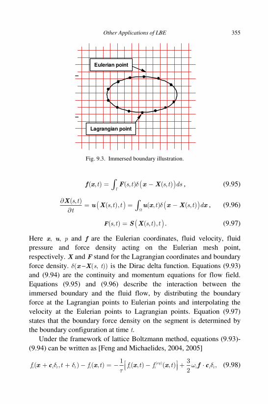
Other Applications of LBE 355
( )( , ) ( , ) ( , )t s t s t dsΓ
= −∫f x F x Xδ , (9.95)
( ) ( )( , )( , ), ( , ) ( , )
s ts t t t s t d
t Ω
∂= = −
∂ ∫X
u X u x x X xδ , (9.96)
( )( , ) ( , ),s t s t t=F S X . (9.97)
Here x, u, p and f are the Eulerian coordinates, fluid velocity, fluid
pressure and force density acting on the Eulerian mesh point,
respectively. X and F stand for the Lagrangian coordinates and boundary
force density. δ(x −X(s, t)) is the Dirac delta function. Equations (9.93)
and (9.94) are the continuity and momentum equations for flow field.
Equations (9.95) and (9.96) describe the interaction between the
immersed boundary and the fluid flow, by distributing the boundary
force at the Lagrangian points to Eulerian points and interpolating the
velocity at the Eulerian points to Lagrangian points. Equation (9.97)
states that the boundary force density on the segment is determined by
the boundary configuration at time t.
Under the framework of lattice Boltzmann method, equations (9.93)-
(9.94) can be written as [Feng and Michaelides, 2004, 2005]
( )1 3( , ) ( , ) ( , ) ( , ) ,
2
eqi i t t i i i i i tf t f t f t f t + + − = − − + ⋅ x x x x fδ δ ω δ
τc c (9.98)
Eulerian point
Lagrangian point
Fig. 9.3. Immersed boundary illustration.

356 Lattice Boltzmann Method and Its Applications in Engineering
where f is the external force density at an Eulerian point, and ωi are
coefficients which depend on the selected lattice velocity model.
Calculation of restoring force
As f is computed from the force density at the boundary point, F, by
using Eq. (9.95), the calculation of F is critical in the application of IBM.
In the following, we will show three ways to compute F.
The first way is the original method of Peskin [1977]. At time t, it is
assumed that the center of mass of the rigid body is at X(t), and the
instantaneous body rotational matrix is R(t). So the position of a
reference point rjX can be determined by
[ ](0) (0)( ) ( ) ( )r rj jt t t= + −X X R X X . (9.99)
For the boundary point tjX which is correspondent to the reference
point rjX , it is allowed to be slightly deformed by the fluid. When the
reference point and the boundary point are not at the same position,
there will be a displacement t rj j j= −X Xξ , and a restoring force Fi is
generated that tends to restore the boundary point back to the reference
point. It can be modeled by a linear spring relation
j jk= −F ξ , (9.100)
where k is the spring constant.
Equation (9.100) is very simple. However, there is a user-defined
parameter k, which may affect the accuracy of numerical solution. To
overcome this drawback, Fadlun et al. [2000] proposed the direct forcing
method. The idea of this way is very simple. Since the boundary point is
also the fluid point, application of Eq. (9.94) at the boundary point
directly gives
pt
∂ = + ⋅ ∇ + ∇ − ∆ ∂u
f u u uρ µ . (9.101)
Suppose that at the time level t = tn, the velocity and pressure fields are
known. At the time level t = tn+1 , the force density at the boundary point
can be calculated by
1
1n ni in n n n n
i i i i ipt
++
− = + ⋅ ∇ + ∇ − ∆ U u
f u u uρ µδ
, (9.102)

Other Applications of LBE 357
where 1n+U is the wall velocity. Note that for the application of
Eq. (9.102), we need to compute the velocity and pressure gradients at
the Eulerian points first, and then interpolate them and the fluid velocity to
the boundary points through Delta function interpolation. The calculation
of derivatives brings inconvenience to the application of IB-LBM.
The third way to compute the restoring force was proposed by Niu
et al. [2006]. It is based on Newton’s second law (the momentum
exchange equals to the impulse). This way is only applicable for
the lattice Boltzmann method. By using Lagrangian interpolated
polynomials, the density distribution functions on the boundary point at
all lattice velocity directions can be calculated by
1, 1,,
( , ) ( , )imax jmax
B kj B imi B i ij
k k i m m ji j ij kj ij im
X x Y yf t f t
x x y y= ≠ = ≠
− − = − − ∑ ∏ ∏X x , (9.103)
where imax and jmax are the maximum numbers of the mesh points in
the x and y directions, respectively. Note that Eq. (9.103) is applied to all
lattice velocity directions. If we view the boundary point from the flow
domain, the lattice velocity directions can be classified as outgoing
directions (from the flow domain to the boundary point) and incoming
directions (from the boundary point to the flow domain). On the other
hand, if we view the boundary point from outside of the flow domain
(inside the object), the lattice velocity directions can also be classified as
outgoing directions (from the boundary point to the flow domain) and
incoming directions (from the flow domain to the boundary point).
Obviously, incoming directions of one view are outgoing directions of
another view. Similarly, outgoing directions of one view are incoming
directions of another view. Therefore, the application of bounce back rule
at the boundary point is equivalent to exchanging the density distribution
functions between a pair of opposite lattice velocity directions. By using
the bounce back rules for the density distribution functions of all
directions, the no-slip boundary condition is satisfied and we have a new
set of distribution functions on the boundary points as shown below,
2
( , ) ( , ) 2 i BB i B i
s
f t f tc
⋅= −
UX X ω ρ
cı , (9.104)
where ı denotes the opposite direction of i ; UB ( ( )B= + × −U X XΩ )
is the velocity of the boundary with U and ΩΩΩΩ representing the translational

358 Lattice Boltzmann Method and Its Applications in Engineering
and angular velocity of the rigid body, and X is the mass center of the
body, XB is its boundary position. Consequently, the boundary force
density can be calculated via the momentum- exchange method, that is,
( , ) ( , ) ( , )B B i Bt f t f t = − − ∑F X X Xc ı ı
ı
. (9.105)
Note that according to Newton’s third law, the hydrodynamic force
exerted on the boundary by the fluids and the force exerted on the fluids
by the boundary have the same magnitude and opposite direction.
δ-function interpolation
The application of Eqs. (9.95) and (9.96) involves the surface and
volume integrals, and continuous δ-function interpolation. In practice, the
integral forms are often replaced by the discrete forms. The two-
dimensional discrete forms can be given by
( , ) ( , ) ( )l lij B ij ij B l
l
t t D s= − ∆∑f x F X x X , (9.106)
,
,( , ) ( ) ( )lij ij ij B
i j
lB t D x yt = − ∆ ∆∑u X u x x X , (9.107)
where ∆sl is the arc length of the boundary element, ∆x and ∆y are
respectively the mesh spacing in the x and y directions. Dij is a kernel
distribution, which can be written as
1
( )l l
ij B ij Blij ij B
x X y YD
x y x y
− − − = ∆ ∆ ∆ ∆ x X δ δ . (9.108)
There are many ways to define the δ-function, and two popular
formulations are given as follows,
( )1
1 cos( | |/2) , | | 2,4
0, | | 2,
r rr
r
+ ≤ = >
πδ (9.109)
( )( )
2
2
13 2 | | 1 4 | | 4 | | , | | 1,
81
5 2 | | 7 12 | | 4 | | , 1 | | 2,( )8
0, | | 2.
r r r r
r r r rr
r
δ
− + + − ≤ − − − + − ≤ ≤= >
(9.110)

Other Applications of LBE 359
For the application of IB-LBM, at first, we need to compute the force
density at the boundary points and then distribute it onto the Eulerian
points. After that, we solve the LBE with the force term f to update the
velocity field. Then we interpolate the new (corrected) velocity field
from the lattice (Eulerian points) to the boundary points and re-calculate
the force density at the boundary point. The process continues until the
convergence criterion is satisfied.
It should be noted that in the conventional IB-LBM, the force density
is pre-calculated. With the known force density f , the new (corrected)
velocity field is explicitly determined. In the process, there is no
guarantee that the velocity at the boundary point obtained from
interpolation of corrected velocity field at Eulerian points equals to the
wall velocity. This means that the no-slip boundary condition may not be
satisfied. This drawback may cause flow penetration to the solid body,
which can be clearly observed in Fig. 9.4.
In the following, we will present a boundary condition-enforced
IB-LBM, in which the force density is considered as an unknown, and is
determined from the no-slip boundary condition.
Fig. 9.4. Flow penetration in the results of conventional IB-LBM for flow around a
circular cylinder (Re = 20).

360 Lattice Boltzmann Method and Its Applications in Engineering
9.4.2 Boundary condition-enforced immersed
boundary-lattice Boltzmann method
We start with the LBE. As shown by Guo et al. [2002a], the LBE with
external force (Eq. (9.98)) cannot properly consider the discrete lattice
effects to the density and momentum. In order to correctly recover the
viscous and incompressible Navier-Stokes equations involving the external
force, the contribution of the force to both momentum ρu and momentum
flux ρuu should be considered. To have a better representation of the
forcing term in LBE, Guo et al. [2002a] proposed a formulation with
higher-order terms in u. With this scheme, the LBE can be written as
( )1( , ) ( , ) ( , ) ( , )eqi t t i i i i tf t f t f t f t F + + − = − − + x e x x xαδ δ δ
τ, (9.111)
2 4
11
2
i ii i i
s s
F wc c
− ⋅ = − + ⋅ ⋅ e u e u
e fτ
, (9.112)
1
2i i t
i
f= +∑u e fρ δ . (9.113)
It can be seen clearly from Eq. (9.113) that the fluid velocity consists of
two parts. One is contributed from the density distribution function
(solution of Eq. (9.111)), and the other is contributed from the force
density f . If we define the intermediate velocity ∗u as
i i
i
f∗ = ∑u eρ , (9.114)
and the velocity correction δu as
1
2t=u fρδ δ , (9.115)
then Eq. (9.113) can be written as
∗= +u u uδ . (9.116)
In the conventional IBM, f is computed in advance. From Eqs. (9.115)
and (9.116), we can see clearly that the velocity correction δu and
corrected velocity u are explicitly calculated. Thus, there is no guarantee
that the velocity at the boundary point interpolated from u satisfies the

Other Applications of LBE 361
no-slip boundary condition. To overcome this drawback, we have to
consider the force density f as an unknown, which is determined in such
a way that the velocity at the boundary point interpolated from u satisfies
the no-slip boundary condition. Similar to Eq. (9.95), the velocity
correction δu at Eulerian points is distributed from the velocity
correction at the boundary (Lagrangian) points. Here, we can set an
unknown velocity correction vector lBuδ at all boundary points. The
velocity correction δu at the Eulerian point can be obtained by the
following Dirac delta function interpolation
( , ) ( , ) ( ( , ))B B Bt t s t dsΓ
= −∫u x u X x Xδ δ δ , (9.117)
The discrete form of Eq. (9.117) can be written as
( , ) ( , ) ( )l l lB B ij ij B l
l
t t D sδ δ= − ∆∑u x u X x X . (9.118)
According to Eq. (9.116), the fluid velocity at Eulerian points can be
corrected as
( , ) ( , ) ( , )ij ij ijt t t∗= +u x u x u xδ , (9.119)
where ( , )ij t∗u x is the intermediate fluid velocity obtained from
Eq. (9.114). Note that the unknowns in Eqs. (9.118) and (9.119) are the
velocity corrections at the boundary points, lBuδ . To satisfy the no-slip
boundary condition, the fluid velocity at the boundary points obtained by
interpolation using the smooth delta function must be equal to the wall
velocity ( , )l
B
lB tU X at the same position. Its mathematical expression is
,
,( , ) ( ) ( )l lB ij ij ij B
i j
lB t D x yt = − ∆ ∆∑U X u x x X . (9.120)
Substituting Eq. (9.119) into Eq. (9.120), we can get the following
equation system
,
,
,
,
( , ) ( ) ( )
( ) ( ) ( ) ,
l lB ij ij ij B
i j
l l l lB B ij ij B l ij ij B
i j l
lB t D
t D s D
t x y
x y
∗= −
− ∆ −
∆ ∆
+ ∆ ∆
∑∑∑
U u x x X
u X x X x X
X
δ
(9.121)
which can be further put as the following matrix form
=AX B , (9.122)

362 Lattice Boltzmann Method and Its Applications in Engineering
where
1
2
B
B
MB
=
δ
δ
δ
u
uX
u
,
1 *11 12 1 1
2 *21 22 2 2
*1 2
B N
B N
MB M M MN N
D D D
D D Dx y
D D D
= − ∆ ∆
U u
U uB
U u
, (9.123)
11 12 1 11 1 12 2 1
21 22 2 21 1 22 2 2
1 2 1 1 2 2
T T TN M M
T T TN M M
T T TM M MN N N NM M
D D D D s D s D s
D D D D s D s D sx y
D D D D s D s D s
∆ ∆ ∆ ∆ ∆ ∆ = ∆ ∆ ∆ ∆ ∆
A
. (9.124)
Here TijD is the element of the transpose matrix of [Dij], M is the number
of Lagrangian (boundary) points and N is the number of the adjacent
Eulerian points around the boundary. Note that the elements of matrix A
are only related to the boundary points and their adjacent Eulerian points.
By solving the above equation system (9.122), we can obtain the
unknown velocity correction at all boundary points. The number of
unknowns in (9.122) is the same as the number of boundary points and
the velocity corrections at all the boundary points can be computed
simultaneously by using a direct method or iterative method to solve
(9.122). After obtaining the velocity correction at the boundary point, the
velocity correction and the corrected velocity at the Eulerian points can
then be calculated by Eqs. (9.118) and (9.119).
Since the no-slip boundary condition is satisfied in the boundary
condition-enforced IB-LBM, the problem of flow penetration is avoided
in its results. This can be seen clearly in Fig. 9.5, which compares the
streamlines for the flow around a circular cylinder at Re = 40 obtained
respectively by the conventional IB-LBM and boundary condition-
enforced IB-LBM.
Another advantage of IB-LBM is the simple calculation of force on
the boundary point. From Eq. (9.115), we can easily compute the force
density (force per area) at the boundary point by
2l lB B t=f uρδ δ . (9.125)

Other Applications of LBE 363
The integration of lBf over the whole surface of the immersed object will
give the total force on the object.
9.5 Summary
As an efficient new numerical method for fluid flows, the LBE has found
wide applications in a variety of complex flows that classical CFD
methods may encounter difficulties. In this chapter we have presented a
brief introduction of the applications in particulate flows, flows in porous
media, turbulent flows, which reveals the potential of LBE in these fields.
We also presented the development of hybrid LBE with the immersed
boundary method for flows with complex geometries or moving objects.
Besides these applications, LBE has also been being employed in many
other areas with successes, such as electronic kinetic flows [e.g., Guo
et al., 2005; He and Li, 2000; Wang and Kang, 2010], magnetohydro-
dynamics [e.g., Breyiannis and Valougeorgis, 2004; Chatterjee and
Amiroudine, 2010; Dellar, 2002], non-Newtonian flows [e.g., Aharonov
and Rothman, 1993; Boek et al., 2003; Yoshino et al., 2007], soft matter
systems [e.g., Dünweg and Ladd, 2009], shallow water flows [e.g., Zhou,
2004], reaction and combustion [Ayodele et al., 2011; Kang et al., 2010;
Machado, 2012; Succi et al., 1997; Filippova and Hänel, 2000], radiation
Fig. 9.5. Streamlines for the flow over a cylinder at Re = 40. Left: Conventional
IB-LBM; Right: Boundary condition-enforced IB-LBM.

364 Lattice Boltzmann Method and Its Applications in Engineering
heat transfer [Asinari et al., 2010; Ma et al., 2011; Mishra and Roy,
2007], relativistic hydrodynamics and quantum mechanics [Dellar et al.,
2011; Mendoza et al., 2010], and so on. Actually, after about two
decades of rapid development, the LBM has achieved much progress in a
wide variety of fields, and the applications are spreading rapidly from the
classical fluid mechanics to other more complex fields. However, there
are still many challenging problems, and it is now still an active research
area.
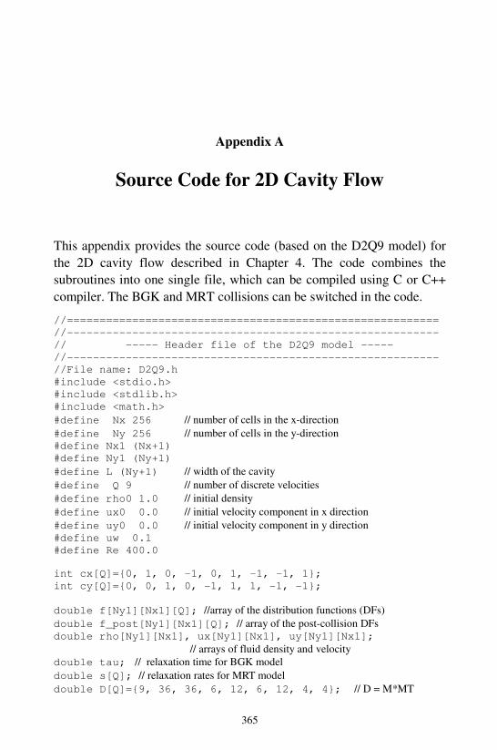
365
Appendix A
Source Code for 2D Cavity Flow
This appendix provides the source code (based on the D2Q9 model) for
the 2D cavity flow described in Chapter 4. The code combines the
subroutines into one single file, which can be compiled using C or C++
compiler. The BGK and MRT collisions can be switched in the code.
//=========================================================
//---------------------------------------------------------
// ----- Header file of the D2Q9 model -----
//---------------------------------------------------------
//File name: D2Q9.h
#include <stdio.h>
#include <stdlib.h>
#include <math.h>
#define Nx 256 // number of cells in the x-direction
#define Ny 256 // number of cells in the y-direction #define Nx1 (Nx+1)
#define Ny1 (Ny+1)
#define L (Ny+1) // width of the cavity
#define Q 9 // number of discrete velocities
#define rho0 1.0 // initial density
#define ux0 0.0 // initial velocity component in x direction
#define uy0 0.0 // initial velocity component in y direction
#define uw 0.1
#define Re 400.0
int cx[Q]=0, 1, 0, -1, 0, 1, -1, -1, 1;
int cy[Q]=0, 0, 1, 0, -1, 1, 1, -1, -1;
double f[Ny1][Nx1][Q]; //array of the distribution functions (DFs)
double f_post[Ny1][Nx1][Q]; // array of the post-collision DFs
double rho[Ny1][Nx1], ux[Ny1][Nx1], uy[Ny1][Nx1];
// arrays of fluid density and velocity
double tau; // relaxation time for BGK model
double s[Q]; // relaxation rates for MRT model
double D[Q]=9, 36, 36, 6, 12, 6, 12, 4, 4; // D = M*MT

366 Lattice Boltzmann Method and Its Applications in Engineering
double w[Q]=4.0/9,1.0/9,1.0/9,1.0/9,1.0/9,1.0/36,1.0/36,
1.0/36,1.0/36; // the weights in the EDF
int rc[Q]=0,3,4,1,2,7,8,5,6; // index of reversed velocity
void Init_Eq(void); //Initialization
double feq(double RHO, double U, double V, int k);
// Equilibrium distribution function
void Coll_BGK(void); // BGK collision
void Coll_MRT(void); // MRT collision
double meq(double RHO, double U, double V, int k);
// Equilibrium momenta
void Streaming(void); // Streaming
void Den_Vel(void); // Fluid variables
void Bounce_back(void); // Bounce-back boundary condition
double Err(void); // Difference in velocity field double u0[Ny1][Nx1],v0[Ny1][Nx1];
void Data_Output(void); // Output simulation data
//=========================================================
//=========================================================
void main()
int k,M2,N2;
double err;
M2=Ny/2; N2=Nx/2;
k=0;
err=1.0;
tau=3*L*uw/Re+0.5; // relaxation time for BGK
s[7]=s[8]=1.0/tau; s[0]=s[3]=s[5]=0.0; s[4]=s[6]=8*(2-
s[7])/(8-s[7]); s[1]=1.6; s[2]=1.8; // relaxation rates for MRT
Init_Eq();
while(err>1.0e-6)
k++;
Coll_BGK(); //BGK collision
// Coll_MRT(); //MRT collision
Streaming(); // Streaming
Bounce_back(); // No-Slip boundary condition
Den_Vel(); // Fluid variables
if(k%1000==0)
err=Err(); // Velocity differences between two successive 1000 steps printf("err=%e ux_center=%e uy_center=%e k=%d\n",err,

Source Code for 2D Cavity Flow 367
ux[M2][N2],uy[M2][N2], k); // Display some results
Data_Output(); // Output simulation data
//=========================================================
//-------------------------------------------------------------------
// Subroutine: initialization with the equilibrium method
//------------------------------------------------------------------
// void Init_Eq()
int j, i, k;
for (j=0;j<=Ny;j++) for(i=0;i<=Nx;i++)
rho[j][i]=rho0;
ux[j][i]=ux0;
uy[j][i]=uy0;
for(k=0;k<Q;k++)
f[j][i][k]=feq(rho[j][i],ux[j][i],uy[j][i],k);
//========================================================
//=========================================================
//-----------------------------------------------------------------
// Subroutine: calculation the equilibrium distribution
//----------------------------------------------------------------
// double feq(double RHO, double U, double V, int k)
double cu, U2;
cu=cx[k]*U+cy[k]*V; // c k*u
U2=U*U+V*V; // u*u; return w[k]*RHO*(1.0+3.0*cu+4.5*cu*cu-1.5*U2);
//=========================================================
//=========================================================
//---------------------------------------------------------
// Subroutine: BGK collision
//--------------------------------------------------------- void Coll_BGK()
int j, i, k;
double FEQ;
for (j=0;j<=Ny;j++) for(i=0;i<=Nx;i++) for(k=0;k<Q;k++)

368 Lattice Boltzmann Method and Its Applications in Engineering
FEQ=feq(rho[j][i],ux[j][i],uy[j][i],k); // EDF
f_post[j][i][k] = f[j][i][k]-(f[j][i][k]-FEQ)/tau;
// Post-collision DFs
//=========================================================
//=========================================================
//---------------------------------------------------------
// Subroutine: MRT collision
//--------------------------------------------------------- void Coll_MRT()
int j, i, k;
double MEQ;
double m[Q];
for (j=0;j<=Ny;j++) for(i=0;i<=Nx;i++)
// Transformation from velocity space to moment space: m[0]=f[j][i][0]+f[j][i][1]+f[j][i][2]+f[j][i][3]+f[j][i]
[4]+f[j][i][5]+f[j][i][6]+f[j][i][7]+f[j][i][8];
m[1]=-4*f[j][i][0]-f[j][i][1]-f[j][i][2]-f[j][i][3]-f[j]
[i][4]+2*(f[j][i][5]+f[j][i][6]+f[j][i][7]+f[j][i
][8]);
m[2]=4*f[j][i][0]-2*(f[j][i][1]+f[j][i][2]+f[j][i][3]+
f[j][i][4])+f[j][i][5]+f[j][i][6]+f[j][i][7]+f[j]
[i][8];
m[3]=f[j][i][1]-f[j][i][3]+f[j][i][5]-f[j][i][6]-
f[j][i][7]+f[j][i][8];
m[4]=-2*(f[j][i][1]-f[j][i][3])+f[j][i][5]-f[j][i][6]-
f[j][i][7]+f[j][i][8];
m[5]=f[j][i][2]-f[j][i][4]+f[j][i][5]+f[j][i][6]-
f[j][i][7]-f[j][i][8];
m[6]=-2*(f[j][i][2]-f[j][i][4])+f[j][i][5]+f[j][i][6]-
f[j][i][7]-f[j][i][8];
m[7]=f[j][i][1]-f[j][i][2]+f[j][i][3]-f[j][i][4];
m[8]=f[j][i][5]-f[j][i][6]+f[j][i][7]-f[j][i][8];
// Relaxation in moment space: for(k=0;k<Q;k++)
MEQ = meq(rho[j][i],ux[j][i],uy[j][i],k);
m[k]= m[k]-s[k]*(m[k]-MEQ); // relaxation
m[k]/=D[k]; // rescaling
// Transforming back to the velocity space: f_post[j][i][0]= m[0]-4*(m[1]-m[2]);
f_post[j][i][1]=m[0]-m[1]-2*(m[2]+m[4])+m[3]+m[7];

Source Code for 2D Cavity Flow 369
f_post[j][i][2]=m[0]-m[1]-2*(m[2]+m[6])+m[5]-m[7];
f_post[j][i][3]=m[0]-m[1]-2*(m[2]-m[4])-m[3]+m[7];
f_post[j][i][4]=m[0]-m[1]-2*(m[2]-m[6])-m[5]-m[7];
f_post[j][i][5]=m[0]+m[1]+m[1]+m[2]+m[3]+m[4]+m[5]+m[6]
+m[8];
f_post[j][i][6]=m[0]+m[1]+m[1]+m[2]-m[3]-m[4]+m[5]+m[6]
-m[8];
f_post[j][i][7]=m[0]+m[1]+m[1]+m[2]-m[3]-m[4]-m[5]-m[6]
+m[8];
f_post[j][i][8]=m[0]+m[1]+m[1]+m[2]+m[3]+m[4]-m[5]-m[6]
-m[8];
//=========================================================
//=========================================================
//---------------------------------------------------------
// Subroutine: calculation the equilibrium moment
//--------------------------------------------------------- double meq(double RHO, double U, double V, int k)
double x;
switch(k)
case 0: x=RHO; break;
case 1: x=RHO*(-2+3*(U*U+V*V));break;
case 2: x=RHO*(1-3*(U*U+V*V));break;
case 3: x=RHO*U;break;
case 4: x=-RHO*U;break;
case 5: x=RHO*V;break;
case 6: x=-RHO*V;break;
case 7: x=RHO*(U*U-V*V);break;
case 8: x=RHO*U*V;break;
default: x=0;
return x;
//=========================================================
//=========================================================
//---------------------------------------------------------
// Subroutine: Streaming
//--------------------------------------------------------- void Streaming()
int j, i, jd, id, k;
for (j=0;j<=Ny;j++) for(i=0;i<=Nx;i++) for(k=0;k<Q;k++)
jd=j-cy[k]; id=i-cx[k]; // upwind node
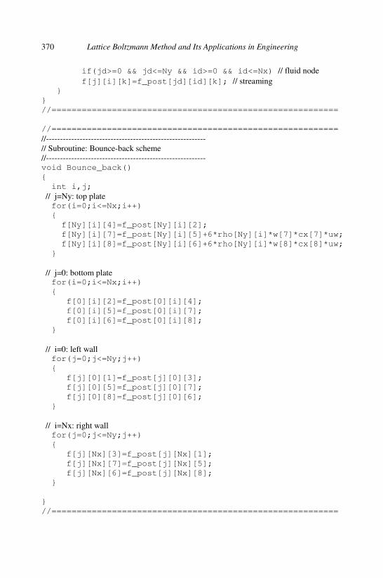
370 Lattice Boltzmann Method and Its Applications in Engineering
if(jd>=0 && jd<=Ny && id>=0 && id<=Nx) // fluid node
f[j][i][k]=f_post[jd][id][k]; // streaming
//=========================================================
//=========================================================
//---------------------------------------------------------
// Subroutine: Bounce-back scheme
//--------------------------------------------------------- void Bounce_back()
int i,j;
// j=Ny: top plate for(i=0;i<=Nx;i++)
f[Ny][i][4]=f_post[Ny][i][2];
f[Ny][i][7]=f_post[Ny][i][5]+6*rho[Ny][i]*w[7]*cx[7]*uw;
f[Ny][i][8]=f_post[Ny][i][6]+6*rho[Ny][i]*w[8]*cx[8]*uw;
// j=0: bottom plate for(i=0;i<=Nx;i++)
f[0][i][2]=f_post[0][i][4];
f[0][i][5]=f_post[0][i][7];
f[0][i][6]=f_post[0][i][8];
// i=0: left wall for(j=0;j<=Ny;j++)
f[j][0][1]=f_post[j][0][3];
f[j][0][5]=f_post[j][0][7];
f[j][0][8]=f_post[j][0][6];
// i=Nx: right wall for(j=0;j<=Ny;j++)
f[j][Nx][3]=f_post[j][Nx][1];
f[j][Nx][7]=f_post[j][Nx][5];
f[j][Nx][6]=f_post[j][Nx][8];
//=========================================================

Source Code for 2D Cavity Flow 371
//=========================================================
//------------------------------------------------------------
// Subroutine: Fluid variables (density and velocity)
//------------------------------------------------------------ void Den_Vel()
int j, i;
for(j=0;j<=Ny;j++) for(i=0;i<=Nx;i++)
rho[j][i]=f[j][i][0]+f[j][i][1]+f[j][i][2]+f[j][i][3]
+f[j][i][4]+f[j][i][5]+f[j][i][6]+f[j][i][7]+
f[j][i][8];
ux[j][i]=(f[j][i][1]+f[j][i][5]+f[j][i][8]-f[j][i][3]-
f[j][i][6]-f[j][i][7])/rho[j][i];
uy[j][i]=(f[j][i][5]+f[j][i][6]+f[j][i][2]-f[j][i][7]-
f[j][i][8]-f[j][i][4])/rho[j][i];
//=========================================================
double Err() // Calculating the relative difference in velocity between two steps
int j, i;
double e1,e2;
e1=e2=0.0;
for(j=1;j<Ny;j++) for(i=0;i<Nx;i++)
e1+=sqrt((ux[j][i]-u0[j][i])*(ux[j][i]-u0[j][i])
+(uy[j][i]-v0[j][i])*(uy[j][i]-v0[j][i]));
e2+=sqrt(ux[j][i]*ux[j][i]+uy[j][i]*uy[j][i]);
u0[j][i]=ux[j][i];v0[j][i]=uy[j][i];
return e1/e2;
void Data_Output() // Output data
int i,j;
FILE *fp;
fp=fopen("x.dat","w+");
for(i=0;i<=Nx;i++) fprintf(fp,"%e \n", (i+0.5)/L);
fclose(fp);
fp=fopen("y.dat","w+");
for(j=0;j<=Ny;j++) fprintf(fp,"%e \n", (j+0.5)/L);
fclose(fp);

372 Lattice Boltzmann Method and Its Applications in Engineering
fp=fopen("ux.dat","w");
for(j=0;j<=Ny;j++)
for (i=0; i<=Nx; i++) fprintf(fp,"%e ",ux[j][i]);
fprintf(fp,"\n");
fclose(fp);
fp=fopen("uy.dat","w");
for(j=0;j<=Ny;j++)
for (i=0; i<=Nx; i++) fprintf(fp,"%e ",uy[j][i]);
fprintf(fp,"\n");
fclose(fp);
fp=fopen("rho.dat","w");
for(j=0;j<=Ny;j++)
for (i=0; i<=Nx; i++) fprintf(fp,"%e ",rho[j][i]);
fprintf(fp,"\n");
fclose(fp);

373
Bibliography
Adler, P. M. (1992). Porous Media: Geometry and Transports (Butterworth, London).
Agrawal, A., Djenidi, L. and Antonia, R. A. (2005). Simulation of gas flow in
microchannels with a sudden expansion or contraction, J. Fluid. Mech., 530,
pp. 135−144.
Aharonov, E. and Rothman, D. (1993). Non-Newtonian flow through porous media: A
lattice-Boltzmann method, Geophys. Res. Lett., 20, pp. 679–682.
Aidun, C. K. and Clausen, J. R. (2010). Lattice-Boltzmann method for complex flows,
Annu. Rev. Fluid Mech., 42, pp. 439–72.
Aidun, C. K. and Lu, Y. (1995). Lattice Boltzmann simulation of solid particles
suspended in fluid, J. Stat. Phys., 81, pp. 49–61.
Aidun, C. K., Lu, Y. and Ding, E. (1998). Direct analysis of particulate suspensions with
inertia using the discrete Boltzmann equation, J. Fluid. Mech., 373, pp. 287–311.
Alexander, F. J., Chen, S. and Grunau, D. W. (1993). Hydrodynamic spinodal
decomposition: Growth kinetics and scaling, Phys. Rev. B, 48, pp. 634–637.
Alexander, F. J., Chen, S. and Sterling, J. D. (1993). Lattice Boltzmann thermo-
hydrodynamics, Phys. Rev. E, 47, pp. R2249–2252.
Amati, G., Succi, S. and Piva, R. (1997). Massively parallel lattice-Boltzmann simulation
of turbulent channel flow, Int. J. Mod. Phys. C, 8, pp. 869–878.
Amati, G., Succi, S. and Piva, R. (1999). Preliminary analysis of the scaling exponents in
channel flow turbulence, Fluid Dyn. Res., 24, pp. 201–209.
Anderson, J. D. (1995). Computational Fluid Dynamics: The Basics with Applications
(McGraw-Hill, New York).
Andries, P., Aoki, K. and Perthame, B. (2002). A consistent BGK-type model for gas
mixtures, J. Stat. Phys., 106, pp. 993–1018.
Arcidiacono, S., Ansumali, S., Karlin, I. V., Mantzaras, J. and Boulouchos, K. B. (2006).
Entropic lattice Boltzmann method for simulation of binary mixtures, Math.
Comput. Simul., 72, pp. 79–83.
Arcidiacono, S., Mantzaras, J., Ansumali, S., Karlin, I. V., Frouzakis, C. E. and
Boulouchos, K. B. (2006). Simulation of binary mixtures with the lattice Boltzman
method, Phys. Rev. E, 74, p. 056707.

374 Lattice Boltzmann Method and Its Applications in Engineering
Arcidiacono, S., Karlin, I. V., Mantzaras, J. and Frouzakis, C. E. (2007). Lattice
Boltzmann model for the simulation of multicomponent mixtures, Phys. Rev. E, 76,
p. 046703.
Aristov, V. V. (2001). Direct Methods for Solving the Boltzmann Equation and Study of
Nonequilibrium Flows (Kluwer Academic, Dordrecht).
Asinari, P. (2005). Viscous coupling based lattice Boltzmann model for binary mixtures,
Phys. Fluids, 17, p. 067102.
Asinari, P. (2006). Semi-implicit-linearized multiple-relaxation-time formulation of
lattice Boltzmann schemes for mixture modeling, Phys. Rev. E, 73, p. 056705.
Asinari, P. and L. S. Luo (2008). A consistent lattice Boltzmann equation with baroclinic
coupling for mixtures, J. Comput. Phys., 227, pp. 3878–3895.
Asinari, P., Mishra, S. C. and Borchiellini, R. (2010). A lattice Boltzmann formulation
for the analysis of radiative heat transfer problems in a participating medium, Num.
Heat Trans. B, 57, pp. 126–146.
Axner, L., Bernsdorf, J., Zeiser, T. et al. (2008). Performance evaluation of a parallel
sparse lattice Boltzmann solver, J. Comput. Phys., 227, pp. 4895–4911.
Ayodele, S. G., Varnik, F. and Raabe, D. (2011). Lattice Boltzmann study of pattern
formation in reaction-diffusion systems, Phys. Rev. E., 83, p. 016702.
Bartoloni, A., Battista, C., Cabasino, S. et al. (1993). LBE simulations of Rayleigh-
Benard convection on the APE100 parallel processor, Int. J. Mod. Phys. C, 4,
pp. 993–1006.
Batchelor, G. K. (1967). An Introduction to Fluid Dynamics (Cambridge University
Press, Cambridge).
Bear, J. (1972). Dynamics of Fluids in Porous Media (Dover, New York).
Benzi, R., Struglia, M. V. and Tripiccione R. (1996). Extended self-similarity in
numerical simulations of three-dimensional anisotropic turbulence, Phys. Rev. E,
53, pp. 5565–5568.
Benzi, R. and Succi, S. (1990). Two-dimensional turbulence with the lattice Boltzmann
equation, J. Phys. A, 23, pp. 1–5.
Benzi, R., Succi, S. and Vergassola, M. (1992). The lattice Boltzmann equation: theory
and applications, Phys. Rep. 222, pp. 145–197.
Bernaschi, M., Rossi, L., Benzi, R. et al. (2009). Graphics processing unit
implementation of lattice Boltzmann models for flowing soft systems, Phys. Rev.
E, 80, p. 066707.
Bernaschi, M. and Succi, S. (2003). Accelerated lattice Boltzmann scheme for steady-
state flows, Int. J. Mod. Phys. B, 17, pp. 1–7.
Bernaschi, M., Succi, S., Chen, H. and Zhang, R. (2002). Computing steady state flows
with an accelerated lattice Boltzmann technique, Int. J. Mod. Phys. C, 13,
pp. 675−687.
Bespalko, D., Pollard, A. and Uddin, M. (2010). Direct numerical simulation of fully-
developed turbulent channel flow using the lattice Boltzmann method and analysis
of openmp scalability, Lect. Notes Comput. Sci., 5976, pp. 1−19.

Bibliography 375
Bhatnagar, P. L., Gross, E. P. and Krook, M. (1954). A model for collision processes in
gases I: small amplitude processes in charged and neutral one-component systems,
Phys. Rev., 94, pp. 511–525.
Bird, G. A. (1994). Molecular Gas Dynamics and the Direct Simulation of Gas Flows
(Clarendon, Oxford).
Boek, E. S., Chin, J. and Coveney, P. V. (2003). Lattice Boltzmann simulation of the
flow of non-Newtonian fluids in porous media, Int. J. Mod. Phys. B, 1, pp. 99–102.
Botella, O. and Peyret, R. (1998). Benchmark spectral results on the lid-driven cavity
flow, Comput. Fluids, 27, pp. 421−433.
Bouzidi, M., Firdaouss, M. and Lallemand, P. (2001). Momentum transfer of a lattice
Boltzmann fluid with boundaries, Phys. Fluids, 13, pp. 3452–3459.
Bouzidi, M., d’Humières, D., Lallemand, P. and Luo, L.-S. (2001). Lattice Boltzmann
equation on a two-dimensional rectangular grid, J. Computat. Phys., 172, pp. 704–
717.
Breyiannis, G. and Valougeorgis, D. (2004). Lattice kinetic simulations in three-
dimensional magnetohydrodynamics, Phys. Rev. E, 69, pp. 65–72
Buick, J. M. and Greated, C. A. (2000). Gravity in a lattice Boltzmann model, Phys. Rev.
E, 61, pp. 5307−5320.
Burattini, P., Lavoie, P., Agrawal, A., Djenidi, L. and Antonia, R. A. (2006). Power law
of decaying homogeneous isotropic turbulence at low Reynolds number, Phys. Rev.
E, 73, p. 066304.
Cao, N., Chen, S. Y., Jin, S. and Martinez, D. (1997). Physical symmetry and lattice
symmetry in the lattice Boltzmann method, Phys. Rev. E, 55, 21–24.
Caiazzo, A. (2005). Analysis of lattice Boltzmann initialization routines, J. Stat. Phys.,
121, pp. 37–48.
Carnahan, N. F. and Starling, K. E. (1969). Equation of state for non-attracting rigid
spheres, J. Chem. Phys., 51, pp. 635–636.
Cercignani, C. (1988). The Boltzmann Equation and Its Applications (Springer-Verlag,
New York).
Chapman, S. and Cowling, T. G. (1970). The Mathematical Theory of Non-Uniform
Gases 3rd Ed. (Cambridge Univ Press, Cambridge, England).
Chatterjee, D. and Amiroudine, S. (2010). Lattice kinetic simulation of nonisothermal
magnetohydrodynamics, Phys. Rev. E, 81, p. 066703.
Chen, F., Xu, A. G., Zhang, G. C., Li, Y. J. and Succi, S. (2010). Multiple-relaxation-
time lattice Boltzmann approach to compressible flows with flexible specific-heat
ratio and Prandtl number, Europhys. Lett., 90, p. 54003.
Chen, F., Xu, A. G., Zhang, G. C. and Li, Y. J. (2011). Multiple-relaxation-time lattice
Boltzmann model for compressible fluids, Phys. Lett. A, 375, pp. 2129–2139.
Chen, H., Kandasamy, S., Orszag, S. A. et al. (2003). Extended Boltzmann kinetic
equation for turbulent flows, Science, 301, pp. 633–636.
Chen, H., Orszag, S. A., Staroselsky, I. and Succi, S. (2004). Expanded analogy
between Boltzmann kinetic theory of fluids and turbulence, J. Fluid Mech., 519,
pp. 301–314.

376 Lattice Boltzmann Method and Its Applications in Engineering
Chen, H., Teixeira, C. and Molvig, K. (1997). Digital physics approach to computational
fluid dynamics: Some basic theoretical features, Int. J. Mod. Phys. C, 8,
pp. 675−684.
Chen, S., Chen, H., Martinez, D. O. and Matthaeus, W. H. (1991). Lattice Boltzmann
model for simulation of magnetohydrodynamics, Phys. Rev. Let., 67, pp. 3776–
3779.
Chen S. and Doolen G. D. (1998). Lattice Boltzmann method for fluid flows, Annu. Rev.
Fluid Mech., 30, pp. 329–64.
Chen, S., Martinez, D. and Mei, R. (1996). On boundary conditions in lattice Boltzmann
methods, Phys. Fluids, 8, pp. 2527–2531.
Chen, S., Wang, Z., Shan, X. W. and Doolen, G. D. (1992). Lattice Boltzmann
computational fluid dynamics in three dimensions, J. Stat. Phys., 68, pp. 379–400.
Chen, Y. and Ohashi, H. (1997). Lattice-BGK methods for simulating incompressible
fluid flows, Int. J. Mod. Phys. C, 8, pp. 793–803.
Chen, Y., Ohashi, H. and Akiyama, M. (1994). Thermal lattice Bhatnagar-Gross-Krook
model without nonlinear deviations in macrodynamic equations, Phys. Rev. E, 50,
pp. 2776−2783.
Chen, Y., Ohashi, H. and Akiyama, M. (1995). Heat transfer in lattice BGK modeled
fluid, J. Stat. Phys., 81, pp. 71−85.
Chen, Y., Ohashi, H. and Akiyama, M. (1997). Two-parameter thermal lattice BGK
model with a controllable Prandtl number, J. Sci. Comput., 12, pp. 169−185.
Cheremisin, F. G. (1991). Fast solutions of the Boltzmann equation, in Rarefied Gas
Dynamics (ed. A. Beylich, VCH, pp. 273).
Chew, Y. T., Shu, C. and Niu, X. D. (2002). A new differential lattice Boltzmann
equation and its application to simulate incompressible flows on non-uniform
grids, J. Stat. Phys., 107, pp. 329−342.
Chew, Y. T., Shu, C. and Peng Y. (2002) On implementation of boundary conditions in
the application of finite volume lattice Boltzmann method, J. Stat. Phys., 107,
pp. 539−556.
Chikatamarla, S. S., Frouzakis, C. E., Karlin, I. V. et al. (2010). Lattice Boltzmann
method for direct numerical simulation of turbulent flows, J. Fluid Mech., 656,
pp. 298–308.
Choi, Y.-H. and Merkle, C. L. (1993). The application of preconditioning to viscous
flows, J. Comput. Phys., 105, pp. 207–233.
Chopard, B. and Masselot, A. (1999). Cellular automata and lattice Boltzmann methods:
a new approach to computational fluid dynamics and particle transport, Future
Generation Comput. Syst., 16, pp. 249–257.
Chun, B. and Ladd, A. J. C. (2007). Interpolated boundary condition for lattice
Boltzmann simulations of flows in narrow gaps, Phys. Rev. E, 75, p. 066705.
Cristea, A. and Sofonea, V. (2003). Reduction of spurious velocity in finite difference
lattice Boltzmann models for liquid–vapor systems, Int. J. Mod. Phys. C, 14,
pp. 1251–1266.

Bibliography 377
Coutanceau, M. and Bouard, R. (1977). Experimental determination of the main features
of the viscous flow in the wake of a circular cylinder in uniform translation. Part 1.
Steady flow, J. Fluid Mech., 79, pp. 231–256.
Crouse, B., Rank, E., Krafczyk, M. and Tölke, J. (2003). A LB-based approach for
adaptive flow simulations, Int. J. Mod. Phys. B, 17, pp. 109−112.
Dardis, O. and McCloskey, J. (1998). Lattice Boltzmann scheme with real numbered
solid density for the simulation of flow in porous media, Phys. Rev. E, 57,
pp. 4834–4837.
Darhuber, A. A. and Troian, S. M. (2005). Principles of microfluidic actuation by
modulation of surface stresses, Annu. Rev. Fluid Mech., 37, pp. 425−455.
Dellar, P. J. (2002), Lattice kinetic schemes for magnetohydrodynamics, J. Comput.
Phys., 179, pp. 95–126.
Dellar, P. J. (2008). Two routes from the Boltzmann equation to compressible flow of
polyatomic gases, Prog. Comput. Fluid Dyn., 8, pp. 84−96.
Dellar, P. J., Lapitski, D., Palpacelli, S. and Succi, S. (2011). Isotropy of three-dimen-
sional quantum lattice Boltzmann schemes, Phys. Rev. E, 83, p. 046706.
Desplat, J.-C., Pagonabarraga, I. and Bladon, P. (2001). LUDWIG: A parallel lattice-
Boltzmann code for complex fluids, Comput. Phys. Commun., 134, pp. 273–290.
d'Humières, D., Lallemand, P. and Frisch, U. (1986). Lattice gas model for 3D
hydrodynamics, Europhys. Lett., 2, p. 291.
d'Humières, D. (1992). Generalized lattice Boltzmann equations, Prog. Aeronaut
Astronaut., 159, pp. 450–458.
d'Humières, D., Ginzburg, I., Krafczyk, M. et al. (2002). Multiple-relaxation-time
lattice Boltzmann models in three dimensions, Phil. Trans. R. Soc. Lond. A, 360,
pp. 437–451.
Ding, H. and Shu, C. (2006). A stencil adaptive algorithm for finite difference solution of
incompressible viscous flows, J. Comput. Phys., 214, pp. 397–420.
Djenidi, L. (2006). Lattice-Boltzmann simulation of grid-generated turbulence, J. Fluid
Mech., 552, pp. 13–35.
Dong, W. (1956). Vacuum flow of gases through channels with circular, annular and
rectangular cross sections. University of California Report, No. UCRL-3353.
Dong, Y.-H., Sagaut, P. and Marie, S. (2008). Inertial consistent sub-grid model for
large-eddy simulation based on the lattice Boltzmann method, Phys. Fluids, 20,
p. 035104.
d'Ortona, U., Salin, D., Cieplak, M., Rybka, R. and Banavar, J. (1995). Two-color
nonlinear Boltzmann cellular automata: Surface tension and wetting, Phys. Rev. E,
51, pp. 3718–3728.
Du, R., Shi, B. C. and Chen, X. W. (2006). Multi-relaxation-time lattice Boltzmann
model for incompressible flow, Phys. Lett.s A, 359, pp. 564–572.
Dünweg, B. and Ladd, A. J. C. (2009). Lattice Boltzmann simulations of soft matter
systems, Adv. Polym. Sci., 221, pp. 89–166.
378 Lattice Boltzmann Method and Its Applications in Engineering
Dupuis, A. and Chopard, B. (2002). Lattice gas modeling of scour formation under
submarine pipelines, J. Comput. Phys., 178, pp. 161–174.
Dupuis, A. and Chopard, B. (2003). Theory and applications of an alternative lattice
Boltzmann grid refinement algorithm, Phys. Rev. E, 67, p. 066707.
Düster, A., Demkowicz, L. and Rank, E. (2006). High-order finite elements applied to the
discrete Boltzmann equation, Int. J. Numer. Meth. Eng. 67, pp. 1094−1121.
Eggels, J. G. M. (1996), Direct and large-eddy simulation of turbulent fluid flow using
the lattice-Boltzmann scheme, Int. J. Heat Fluid Flow, 17, pp. 307–323.
Eggels, J. G. M. and Somers, J. A. (1995). Numerical simulation of the free convective
flow using the lattice-Boltzmann scheme, Int. J. Heat Fluid Flow, 16, pp. 357–364.
Ergun, S. (1952). Flow through packed columns, Chem. Eng. Prog., 48, pp. 89–94.
Fadlun, E., Verzicco, R., Orlandi, P., Mohd-Yusof, J. (2000). Combined immersed-
boundary finite-difference methods for three dimensional complex flow simulations,
J. Comput. Phys., 161, pp. 35–60.
Feng, Y. T., Han, K. and Owen, D. R. J. (2007). Coupled lattice Boltzmann method and
discrete element modelling of particle transport in turbulent fluid flows:
Computational issues, Int. J. Numer. Meth. Engng., 72, pp. 1111–1134.
Feng, Z. and Michaelides, E. (2004). The immersed boundary-lattice Boltzmann
method for solving fluid-particles interaction problems, J. Comput. Phys., 195,
pp. 602–628.
Feng, Z. and Michaelides, E. (2005). Proteus: a direct forcing method in the simulations
of particulate flows, J. Comput. Phys., 202, pp. 20–51.
Ferzige, J. H. and Peric, M. (2002). Computational Methods for Fluid Dynamics 3rd Ed.
(Springer-Verlag, Berlin).
Filippova, O. and Hänel, D. (1997). Lattice-Boltzmann simulation of gas-particle flow in
filters, Comput. Fluids, 26, pp. 697−712.
Filippova, O. and Hänel, D. (1998). Grid refinement for lattice-BGK models, J. Comput.
Phys., 147, pp. 219–228.
Filippova, O. and Hänel, D. (2000). A novel lattice BGK approach for low Mach number
combustion, J. Comput. Phys., 158, pp. 139–160.
Filippova, O., Succi, S., Mazzocco, F. et al. (2001). Multiscale Lattice Boltzmann
Schemes with Turbulence Modeling, J. Comput. Phys., 170, pp. 812–829.
Flekkøy, E. G. (1993). Lattice Bhatnagar-Gross-Krook models for miscible fluids, Phys.
Rev. E, 47, pp. 4247–4257.
Frisch, U., Hasslacher, B. and Pomeau, Y. (1986). Lattice-gas automata for the Navier-
Stokes equations, Phys. Rev. Lett., 56, pp. 1505–1508.
Frisch, U., d'Humiéres, D., Hasslacher, B. et al. (1987). Lattice gas hydrodynamics in
two and three dimensions, Complex Syst., 1, pp. 649–707.
Gan, Y. B., Xu, A. G., Zhang, G. C. et al. (2008). Two-dimensional lattice Boltzmann
model for compressible flows with high Mach number, Physica. A, 387,
pp. 1721−1732.

Bibliography 379
Ghia, U., Ghia, K. N. and Shin, C. T. (1982). High resolution of Navier-Stokes equations
in primitive variables, J. Comput. Phys., 48, pp. 387−411.
Ginzbourg, I. and Adler, P. M. (1994). Boundary flow condition analysis for the three-
dimensional lattice Boltzmann model, J. Phys. II. France, 4, pp. 191–214.
Ginzbourg, I. and d'Humières, D. (2003). Multireflection boundary conditions for lattice
Boltzmann models, Phys. Rev. E, p. 066614.
Girimaji, S. S. (2007). Boltzmann kinetic equation for filtered fluid turbulence, Phys. Rev.
Lett., 99, p. 034501.
Goldstein, D., Hadler, R. and Sirovich, L. (1993). Modeling a no-slip flow boundary with
an external force field, J. Comput. Phys., 105, pp. 354–366.
Gross E. P. and Krook, M. (1956). Models for collision process: Small-amplitude
oscillations of charged two-component systems, Phys. Rev., 102, pp. 593–604.
Grunau, D., Chen, S. and Eggert, K. (1993). A lattice Boltzmann model for multiphase
fluid flows, Phys. Fluids A, 5, pp. 2557–2562.
Gunstensen, A. K. and Rothman, D. H. (1993). Lattice Boltzmann studies of immiscible
two phase flow through porous media, J. Geophys. Res., 98, pp. 6431–6341.
Gunstensen, A. K., Rothman, D. H., Zaleski, S. and Zanetti, G. (1991). Lattice
Boltzmann model of immiscible fluids, Phys. Rev. A, 43, pp. 4320–4327.
Guo, Z. L., Asinari, P. and Zheng, C. G. (2009). Lattice Boltzmann equation for
microscale gas flows of binary mixtures, Phys. Rev. E, 79, p. 026702.
Guo, Z. L., Shi, B. C. and Wang, N. C. (2000). Lattice BGK model for incompressible
Navier-Stokes equation, J. Comput. Phys., 165, pp. 288–306.
Guo, Z. L., Shi, B. C., Zhao, T. S. and Zheng, C. G. (2007). Discrete effects on boundary
conditions for the lattice Boltzmann equation in simulating microscopic gas flows,
Phys. Rev. E, 76, p. 056704.
Guo, Z. L., Shi, B. C. and Zheng C. G. (2002). A coupled lattice BGK model for the
Boussinesq equations, Int. J. Numer. Meth. Fluids, 39, pp. 325–342.
Guo, Z. L., Shi, B. C. and Zheng, C. G. (2007). An extended Navier-Stokes formulation
for gas flows in Knudsen layer near a wall, Europhys. Lett., 80, p. 24001.
Guo, Z. L., Shi, B. C. and Zheng, C. G. (2011). Chequerboard effects on spurious
currents in the lattice Boltzmann equation for two-phase flows, Phil. Trans. R. Soc.
A, 369(1944), pp. 2283–2291.
Guo, Z. L. and Zhao, T. S. (2002). Lattice Boltzmann method for flow through porous
media, Phys. Rev. E, 66, p. 036304.
Guo, Z. L. and Zhao, T. S. (2003a). Explicit finite-difference lattioce Boltzmann method
for curvilinear coordinates, Phys. Rev. E, 67, p. 066709.
Guo, Z. L. and Zhao, T. S. (2003b). Discrete velocity and lattice Boltzmann models for
binary mixtures of nonideal fluids, Phys. Rev. E, 68, p. 035302.
Guo, Z. L. and Zhao, T. S. (2005). Finite-difference-based lattice Boltzmann model for
dense binary mixtures, Phys. Rev. E, 71, p. 026701.
Guo, Z. L., Zhao, T. S. and Shi, Y. (2004). Preconditioned lattice-Boltzmann method for
steady flows, Phys. Rev. E, 70, p. 066706.

380 Lattice Boltzmann Method and Its Applications in Engineering
Guo, Z. L., Zhao, T. S. and Shi, Y. (2005). A lattice Boltzmann algorithm for electro-
osmotic flows in microfluidic devices, J. Chem. Phys., 122, p. 144907.
Guo, Z. L., Zhao, T. S. and Shi, Y. (2006). Physical symmetry, spatial accuracy, and
relaxation time of the lattice Boltzmann equation for micro gas flows, J. Appl.
Phys., 99, p. 074903.
Guo, Z. L. and Zheng, C. G. (2007). Analysis of lattice Boltzmann equation for
microscale gas flows: Relaxation times, boundary conditions and the Knudsen
layer, Int. J. Comput. Fluid Dynamics, 22, pp. 465−43.
Guo, Z. L., Zheng, C. G. and Shi, B. C. (2002a). Non-equilibrium extrapolation method
for velocity and pressure boundary conditions in the lattice Boltzmann method,
Chinese Phys., 11, pp. 366–374.
Guo, Z. L., Zheng, C. G. and Shi, B. C. (2002b). An extrapolation method for boundary
conditions in lattice Boltzmann method, Phys. Fluids, pp. 2007–2010.
Guo, Z. L., Zheng, C. G. and Shi, B. C. (2002c). Discrete lattice effects on the forcing
term in the lattice Boltzmann method, Phys. Rev. E, 65, p. 046308.
Guo, Z. L., Zheng, C. G. and Shi, B. C. (2003). Domain decomposition technique in
lattice Boltzmann method, Int. J. Mod. Phys. B, 17, pp. 129–133.
Guo, Z. L., Zheng, C. G. and Shi, B. C. (2007). Thermal lattice Boltzmann equation for
low Mach number flows: Decoupling mode, Phys. Rev. E, 75, p. 36704.
Guo, Z. L., Zheng, C. G. and Shi, B. C. (2008). Lattice Boltzmann equation with
multiple effective relaxation times for gaseous microscopic flow, Phys. Rev. E, 77,
p. 036707.
Guo, Z. L., Zheng, C. G. and Shi, B. C. (2011). Force imbalance in lattice Boltzmann
equation for two-phase flows, Phys. Rev. E, 83, p. 036707.
Guo, Z. L. and Zhou, Y. (2004). Numerical simulation of oscillating-cylinder effects on a
downstream cylinder wake using lattice Boltzmann method, Fluid Mech. its Appl.,
75, pp. 415–424.
Hadjiconstantinou, N. G. (2003). Comment on Cercignani's second-order slip coefficient,
Phys. Fluids, 15, pp. 2352−2354.
Hamel, B. B. (1966). Two fluid hydrodynamic equations for a neutral, disparate, mass,
binary mixture, Phys. Fluids, 9, pp. 12–22.
Hardy, J., Pomeau, Y. and de Pazzis O. (1973a). Time evolution of a two-dimensional
classical lattice system, Phys. Rev. Lett., 31, pp. 276–279.
Hardy, J., Pomeau, Y. and de Pazzis O. (1973b). Time evolution of two-dimensional
model system I: Invarient states and time correlation functions, J. Math. Phys., 14,
1746–1759.
Harris, S. (1971). An Introduction to the Theory of the Boltzmann Equation (Holt,
Rinehart and Winston, New York).
Hatiboglu, C. U. and Babadagli, T. (2007). Lattice-Boltzmann simulation of solvent
diffusion into oil-saturated porous media, Phys. Rev. E, 76, p. 066309.
Hatiboglu, C. U. and Babadagli, T. (2008). Pore-scale studies of spontaneous imbibition
into oil-saturated porous media, Phys. Rev. E, 77, p. 066311.

Bibliography 381
Házi, G. and Tóth, G. (2010). Lattice Boltzmann simulation of two-dimensional wall
bounded turbulent flow, Int. J. Mod. Phys. C, 21, pp. 669–680.
He, X., Chen, S. and Doolen, G. D. (1998). A novel thermal model for the lattice
Boltzmann method in incompressible limit, J. Comput. Phys., 146, pp. 282–300.
He, X., Chen, S. and Zhang, R. (1999). A lattice Boltzmann scheme for incompressible
multiphase flow and its application in simulation of Rayleigh-Taylor instability,
J. Comput. Phys., 152, pp. 642–663.
He, X. and Doolen, G. (1997). Lattice Boltzmann method on curvilinear coordinates
system: Flow around a circular cylinder, J. Comput. Phys., 134, pp. 306–315.
He, X., Doolen, G. D. and Clark, T. (2002). Comparison of the lattice Boltzmann method
and the artificial compressibility method for Navier-Stokes equations, J. Comput.
Phys., 179, 439–451.
He, X. and Li, N. (2000). Lattice Boltzmann simulation of electrochemical systems,
Comput. Phys. Comm., 129, pp. 158–166.
He, X. and Luo, I.-S. (1997). Lattice Boltzmann model for the incompressible Navier-
Stokes equation, J. Stat. Phys., 88, pp. 927–944.
He, X., Luo, L.-S. and Dembo, M. (1996). Some progress in lattice Boltzmann method 1:
Nonuniform mesh grids, J. Comput. Phys., 29, pp. 357–363.
He, X., Zou, Q., Luo, L.-S. and Dembo, M. (1997). Analytic solutions of simple flow and
analysis of non-slip boundary conditions for the lattice Boltzmann BGK model,
J. Stat. Phys., 87, pp. 115–123.
He, X., Luo, L.-S. and Dembo, M. (1997). Some progress in the lattice Boltzmann
method: Reynolds number enhancement in simulations, Phys. A, 239, pp. 276–285.
He, X., Shan, X. and Doolen, G. D. (1998). Discrete Boltzmann equation model for
nonideal gases, Phys. Rev. E, 57, pp. 13–16.
He, X., Zhang, R., Chen, S. and Doolen, G. D. (1999). On the three-dimensional
Rayleigh-Taylor instability, Phys. Fluids, 11, pp. 1143–1152.
He, X., Zou, Q., Luo, L. S. and Dembo, M. (1997). Analytic solutions of simple flow and
analysis of non-slip boundary conditions for the lattice Boltzmann BGK model,
J. Stat. Phys., 87, pp. 115−123.
Heijs, A. and Lowe, C. P. (1995). Numerical evaluation of the permeability and the
Kozeny constant for two types of porous media, Phys. Rev. E, 51, pp. 4346–4352.
Higuera, F. and Jimenez, J. (1989). Boltzmann approach to lattice gas simulations,
Europhys. Lett., 9, pp. 663–668.
Higuera, F. J. and Succi, S. (1989). Simulating the flow around a circular cylinder with a
lattice Boltzmann equation, Europhys. Lett., 8, pp. 517–521.
Higuera, F., Succi, S. and Benzi, R. (1989). Lattice gas dynamics with enhanced
collisions, Europhys. Lett., 9, pp. 345–349.
Ho, C.-M. and Tai, Y.-C. (1998). Micro-electro-mechanicalsystems (MEMS) and fluid
flows, Annu. Rev. Fluid Mech., 30, pp. 579−612.
Holway, L. H. (1966). New statistical models for kinetic theory: methods of construction,
Phys. Fluids, 9, pp. 1658–1673.

382 Lattice Boltzmann Method and Its Applications in Engineering
Hoogerbrugge, P. J. and Koelman, J. (1992). Simulating microscopic hydrodynamic
phenomena with dissipative particle dynamics, Europhys. Lett., 19, pp. 155–160.
Hou, S., Shan, X., Zou, Q., Doolen, G. D. and Soll, W. E. (1997). Evaluation of two
lattice Boltzmann models for multiphase flows, J. Comput. Phys., 138, pp. 695–
713.
Hou, S., Sterling, J., Chen, S. and Doolen, G. D. (1996). A lattice Boltzmann sub-grid
model for high Reynolds number flows, Fields Inst. Comm., 6, pp. 151–166.
Hou, S. and Zou, Q. (1995). Simulation of cavity flow by the lattice Boltzmann method,
J. Comput. Phys., 118, pp. 329–347.
Hu, S. X., Yan, G. W. and Shi, W. P. (1997). A lattice Boltzmann model for
compressible perfect gas, Acta Mech. Sinica, 13, pp. 218–226.
Inamuro, T., Konishi, N. and Ogino, F. (2000). A Galilean invariant model of the lattice
Boltzmann method for multiphase fluid flows using free-energy approach, Comput.
Phys. Commun, 129, pp. 32–45.
Inamuro, T., Maeba, K. and Ogino, F. (2000). Flow between parallel walls containing
the lines of neutrally buoyant circular cylinders, Int. J. Multiphase Flow, 26,
pp. 1981–2004.
Inamuro, T., Ogata, T., Tajima, S. and Konishi, N. (2004). A lattice Boltzmann method
for incompressible two-phase flows with large density differences, J. Comput.
Phys., 198, pp. 628–644.
Inamuro, T., Yoshino, M. and Ogino, F. (1995). A non-slip boundary condition for lattice
Boltzmann simulations, Phys. Fluids, 7, pp. 2928–2930.
Inamuro, T., Yoshino, M. and Ogino, F. (1999). Lattice Boltzmann simulation of
flows in a three-dimensional porous structure, Int. J. Numer. Meth. Fluids, 29,
pp. 737–748.
Ivchenko, I. N., Loyalka, S. K. and Tompson, R. V. (1997). Slip coefficients for binary
gas mixtures, J. Vac. Sci. Tech. A, 15, pp. 2375−2371.
Izquierdo, S. and Fueyo, N. (2008). Preconditioned Navier-Stokes schemes from the
generalised lattice Boltzmann equation, Prog. Comput. Fluid Dyn., 8, pp. 189−196.
Izquierdo, S. and Fueyo, N. (2009). Optimal preconditioning of lattice Boltzmann
method, J. Comput. Phys., 228, pp. 6479–6495.
Jafari, S. and Rahnama, M. (2011). Shear-improved Smagorinsky modeling of turbulent
channel flow using generalized lattice Boltzmann equation, Int. J. Numer. Meth.
Fluids, 67, pp. 700–712.
Jameson, A., Schmidt, W. and Turkel, E. (1981). Numerical solution of the Euler
equations by finite volume methods using Runge-Kutta time-stepping scheme,
AIAA paper 81−1259.
Ji, C. Z., Shu, C. and Zhao, N. (2009). A lattice Boltzmann method-based flux solver and
its application to solve shock tube problem, Mod. Phys. Lett. B, 23, pp. 313–316.
Joshi, H., Agarwal, A., Puranik, B., Shu, C. and Agrawal, A. (2010). A hybrid FVM-
LBM method for single and multi-fluid compressible flow problems, Int J. Numer.
Meth. Fluid, 62, pp. 403–427.

Bibliography 383
Junk, M. and Yang, Z. X. (2005a). Asymtotic analysis of lattice Boltzmann boundary
conditions, J. Stat. Phys., 121, pp. 3–35.
Junk, M. and Yang, Z. X. (2005b). One-point boundary condition for the lattice
Boltzmann method, Phys. Rev. E, 72, p. 066701.
Kalarakis, A., Burganos, V. and Payatakes, A. C. (2002). Galilean-invariant lattice-
Boltzmann simulation of liquid-vapor interface dynamics, Phys. Rev. E, 65,
p. 056702.
Kang, Q., Lichtner, P. C. and Janecky, D. R. (2010). Lattice Boltzmann method for
reacting flows in porous media, Adv. Appl. Math. Mech., 2, pp. 545–563.
Kandhai, D., Koponen, A., Hoekstra, A. et al. (1998). Lattice-Boltzmann hydrodynamics
on parallel systems, Comp. Phys. Comm., 111, pp. 14–26.
Kandhai, D., Koponen, A., Hoekstra, A. et al. (1999). Implementation aspects of 3D
lattice-BGK: boundaries, accuracy, and a new fast relaxation method, J. Comput.
Phys., 150, pp. 482–501.
Kanki, T. and Iuchi, S. (1973). Poiseuille flow and thermal creep of a rarefied gas
between parallel plates, Phys. Fluids, 16, pp. 594–599.
Kao, P.-H. and Yang, R.-J. (2008). An investigation into curved and moving boundary
treatments in the lattice Boltzmann method, J. Comput. Phys., 227, pp. 5671–5690.
Karniadakis, G. E. and Beskok, A. (2002) Micro Flows (Springer-Verlag, New York).
Kataoka, T. and Tsutahara, M. (2004a). Lattice Boltzmann method for the compressible
Navier-Stokes equations with flexible specific-heat ratio, Phys. Rev. E, 69,
p. R035701.
Kataoka, T. and Tsutahara, M. (2004b). Lattice Boltzmann method for the compressible
Euler equations, Phys. Rev. E, 69, p. 056702.
Kim, W. T., Jhon, M. S., Zhou, Y. et al. (2005). Nanoscale air bearing modeling via
lattice Boltzmann method, J. Appl. Phys., 97, p. 10P304.
Koelman, J. (1991). A simple lattice Boltzmann scheme for Navier-Stokes fluid flow,
Europhys. Lett., 15, pp. 603–607.
Koponen, A., Kandhai, D., Hellén, E. et al. (1998). Permeability of three-dimensional
random fiber webs, Phys. Rev. Lett., 80, pp. 716–719.
Krafczyk, M., Tölke, J. and Luo, L.-S. (2003). Large-eddy simulations with a multiple-
relaxation- time LBE model, Int. J. Mod. Phys. B, 7, pp. 33–39.
Ladd, A. J. C. (1994a). Numerical simulations of particulate suspensions via a discretized
Boltzmann equation. Part I. Theoretical foundation, J. Fluid Mech., 271, pp. 285–
310.
Ladd, A. J. C. (1994b). Numerical simulations of particulate suspensions via a discretized
Boltzmann equation. Part II. Numerical results, J. Fluid Mech., 271, pp. 311–339.
Ladd, A. J. C. and Verberg, R. (2001). Lattice-Boltzmann simulations of particle-fluid
suspensions, J. Stat. Phys., 104, pp. 1191–1251.
Lai, Y. G., Lin, C. L. and Huang, J. C. (2001). Accuracy and efficiency study of lattice
Boltzmann method for steady-state flow simulations, Num. Heat Transf. Part B,
39, pp. 21–43.

384 Lattice Boltzmann Method and Its Applications in Engineering
Lai, M. C. and Peskin, C. S. (2000). An immersed boundary method with formal second-
order accuracy and Reduced numerical viscosity, J. Comput. Phys., 160, pp. 705–
719.
Lallemand, P. and Luo, L.-S. (2000). Theory of the lattice Boltzmann method:
Dispersion, dissipation, isotropy, Galilean invariance, and stability, Phys. Rev. E,
61, pp. 6546–6562.
Lallemand, P. and Luo, L.-S. (2003). Theory of the lattice Boltzmann method: Acoustic
and thermal properties in two and three dimensions, Phys. Rev. E, 68, pp. 036706.
Lammers, P., Beronov, K. N., Volkert, R. et al. (2006). Lattice BGK direct numerical
simulation of fully developed turbulence in incompressible plane channel flow,
Comput. Fluids, 35, pp. 1137–1153.
Lantermann, U. and Hänel, D. (2007). Particle Monte Carlo and lattice-Boltzmann
methods for simulations of gas-particle flows, Comput. Fluids, 36, pp. 407–422.
Lee, D. (1996). Local Preconditioning of the Euler and the Navier-Stokes Equations.
Ph.D. thesis, University of Michigan.
Lee, T. and Fischer, P. F. (2006). Eliminating parasitic currents in the lattice Boltzmann
equation method for nonideal gases, Phys. Rev. E, 74, p. 046709.
Lee, T. and Lin, C.-L. (2001). A characteristic Galerkin method for discrete Boltzmann
equation, J. Comput. Phys., 171, pp. 336–356.
Lee, T. and Lin, C. L. (2003). An Eulerian description of the streaming process in the
lattice Boltzmann equation, J. Comput. Phys., 185, pp. 445–471.
Lee, T. and Lin, C.-L. (2005a). A stable discretization of the lattice Boltzmann equation
for simulation of incompressible two-phase flows at high density ratio, J. Comput.
Phys., 2106, pp. 16–47.
Lee, T. and Lin, C. L. (2005b). Rarefaction and compressibility effects of the lattice
Boltzmann equation method in a gas microchannel, Phys. Rev. E, 71, p. 046706.
Li, H. B., Lu, X., Fang, H. P. and Qian, Y. H. (2004). Force evaluations in lattice
Boltzmann simulations with moving boundaries in two dimensions, Phys. Rev. E,
70, p. 026701.
Li, Q., He, Y. L., Wang, Y. and Tao, W. Q. (2007). Coupled double-distribution-function
lattice Boltzmann method for the compressible Navier-Stokes equations, Phys.
Rev. E, 76, p. 056705.
Li, Q., He, Y. L., Wang, Y. and Tang, G. H. (2009). Three-dimensional non-free-
parameter lattice-Boltzmann model and its application to inviscid compressible
flows, Phys. Lett. A, 373, pp. 2101–2108.
Li, W., Wei, X. M. and Kaufman, A. (2004). Implementing lattice Boltzmann
computation on graphics hardware, Visual Comput., 19, pp. 444–445.
Li, Y., LeBoeuf, E. J. and Basu, P. K. (2004). Least-squares finite-element lattice
Boltzmann method, Phys. Rev. E, 69, p. 065701.
Lim, C. Y., Shu, C., Niu, X. D. and Chew, Y. T. (2002). Application of lattice Boltzmann
method to simulate microchannel flows, Phys. Fluids, 14, pp. 2299−2308.

Bibliography 385
Lin, Z., Fang, H. P. and Tao, R. B. (1996). Improved lattice Boltzmann model for
incompressible two-dimensional steady flows, Phys. Rev. E, 54, pp. 6323–6330.
Liu, H. J., Zou, C., Shi, B. C. et al. (2006). Thermal lattice-BGK model based on large-
eddy simulation of turbulent natural convection due to internal heat generation, Int.
J. Heat Mass Transf., 49, pp. 4672–4680.
Lockerby, D. A., Reese, J. M. and Gallis, M. A. (2005). The usefulness of higher-order
constitutive relations for describing the Knudsen layer, Phys. Fluids, 17, p. 100609.
Lowe, C., Frenkel, D. and Masters, A. J. (1995). Long-time tails in angular momentum
correlations, J. Chem. Phys., 103, pp. 1582–1587.
Lu, X.-Y. and Dalton, C. (1996). Calculation of the timing of vortex formation from an
oscillating cylinder, J. Fluids Struct., 10, pp. 527–541.
Lu, Z., Liao, Y., Qian, D. et al. (2002). Large eddy simulations of a stirred tank using
the lattice Boltzmann method on a nonuniform grid, J. Comput. Phys., 181,
pp. 675–704.
Luis, V., Jesus, M. and Gabor, H. (2010). Dynamics of isotropic homogeneous turbulence
with linear forcing using a lattice Boltzmann method, Flow Turb. Combust., 84,
pp. 219–237.
Luo, L.-S. (1997). Analytic solutions of linearized lattice Boltzmann equation, J. Stat.
Phys., 88, pp. 913–926.
Luo, L.-S. (1998). Unified theory of the lattice Boltzmann models for nonideal gases,
Phys. Rev. Lett., 81, pp. 1618–1621.
Luo, L. (2000). Theory of the lattice Boltzmann method: Lattice Boltzmann models for
nonideal gases, Phys. Rev. E, 62, pp. 4982–4996.
Luo, L. S. (2004). Comment on “Discrete Boltzmann equation for microfluidics”,
Phys. Rev. Lett., 92, p. 139401.
Luo, L.-S., Liao, W., Chen, X. W. et al. (2011). Numerics of the lattice Boltzmann
method: Effects of collision models on the lattice Boltzmann simulations,
Phys. Rev. E, 83, p. 056710.
Luo, L. S. and Girimaji, S. S. (2002). Lattice Boltzmann model for binary mixtures,
Phys. Rev. E, 66, p. 035301.
Luo, L. S. and Girimaji, S. S. (2003). Theory of the lattice Boltzmann method: Two-fluid
model for binary mixtures, Phys. Rev. E, 67, p. 036302.
Ma, Y., Dong, S. and Tan, H. P. (2011). Lattice Boltzmann method for one-dimensional
radiation transfer, Phys. Rev. E, 84, p. 016704.
Machado, R. (2012). Numerical simulations of surface reaction in porous media with
lattice Boltzmann, Chem. Eng. Sci., 69, pp. 628–643.
Madadi, M. and Sahimi, M. (2003). Lattice Boltzmann simulation of fluid flow in
fracture networks with rough, self-affine surfaces, Phys. Rev. E, 67, p. 026309.
Maier, R. S., Bernard, R. S. and Grunau, D. W. (1996). Boundary conditions for the
lattice Boltzmann method, Phys. Fluids, 8, pp. 1788–1793.
Maier, R. S., Kroll, D. M., Benard, R. S. et al. (2000). Pore-scale simulation of dispersion,
Phys. Fluids, 12, pp. 2065–2079.

386 Lattice Boltzmann Method and Its Applications in Engineering
Malaspinas, O. and Sagaut, P. (2011). Advanced large-eddy simulation for lattice
Boltzmann methods: The approximate deconvolution model, Phys. Fluids, 23,
p. 105103.
Manz, B., Gladden, L. F. and Warren, P. B. (1999). Flow and dispersion in porous
media: Lattice-Boltzmann and NMR studies, AIChE J., 45, pp. 1845–1854.
Martinez, D. O., Matthaeus, W. H., Chen, S. and Montgomery, D. C. (1994). Comparison
of spectral method and lattice Boltzmann simulations of two-dimensional
hydrodynamics, Phys. Fluids, 6, pp. 1285–1298.
Martys, N. S. (2001). Improved approximation of the Brinkman equation using a lattice
Boltzmann method, Phys. Fluids, 6, pp. 1807–1810.
Martys, N. S. and Chen, H. (1996). Simulation of multicomponent fluids in complex
three-dimensional geometries by the lattice Boltzmann method, Phys. Rev. E, 53,
pp. 743–750.
Martys, N. S., Shan, X. and Chen, H. (1998). Evaluation of the external force term in the
discrete Boltzmann equation, Phys. Rev. E, 58, pp. 6855–6857.
Masselot, A. and Chopard, B. (1998). A lattice Boltzmann model for particle transport
and deposition, Europhys. Lett., 42, pp. 259–264.
Mattila, K., Hyvaluoma, J., Rossi, T. et al. (2007). An efficient swap algorithm for the
lattice Boltzmann method, Comput. Phys. Commun., 176, pp. 200–210.
Mavriplis, D. (2006). Multigrid solution of the steady-state lattice Boltzmann equation,
Comp. Fluids, 35, pp. 793804.
Mayer, G., Páles, J. and Házi, G. (2007). Large eddy simulation of subchannels using the
lattice Boltzmann method, Ann. Nucl. Energy, 34, pp. 140–149.
McCracken, M. E. and Abraham, J. (2005). Lattice Boltzmann methods for binary
mixtures with different molecular weights, Phys. Rev. E, 71, p. 046704.
McNamara, G. R., Garcia, A. L. and Alder, B. J. (1995). Stabilization of thermal lattice
Boltzmann models, J. Stat. Phys., 81, pp. 395–408.
McNamara, G. R., Garcia, A. L. and Alder, B. J. (1997). A hydrodynamically correct
thermal lattice Boltzmann model, J. Stat. Phys., 87, pp. 1111–1121.
McNamara, G. R. and Zanetti, G. (1988). Use of the Boltzmann equation to simulate
lattice gas automata, Phys. Rev. Lett., 61, pp. 2332–2335.
Mei, R., Luo, L.-S., Lallemand, P. and d'Humières, D. (2006). Consistent initial
conditions for lattice Boltzmann simulations, Comput. Fluids, 35, 855–862.
Mei, R., Luo, L.-S. and Shyy, W. (1999). An accurate curved boundary treatment in the
lattice Boltzmann method, J. Comput. Phys., 155, pp. 307–330.
Mei, R. and Shyy, W. (1998). On the finite difference-based lattice Boltzmann method in
curvilinear coordinates, J. Comput. Phys., 143, pp. 426–448.
Mei, R., Yu, D. and Shyy, W. (2002). Force evaluation in lattice Boltzmann method
involving curved geometry, Phys. Rev. E, 65, p. 041203.
Mendoza, M., Boghosian, B. M., Herrmann1, H. J. and Succi, S. (2010). Fast lattice
Boltzmann solver for relativistic hydrodynamics, Phys. Rev. Lett., 105, p. 014502.

Bibliography 387
Menon, S. and Soo, J.-H. (2004). Simulation of vortex dynamics in three-dimensional
synthetic and free jets using the large-eddy lattice Boltzmann method, J. Turb., 5,
pp. 1–26.
Mezrhab, A., Bouzidi, M. and Lallermand, P. (2004). Hybrid lattice-Boltzmann finite-
difference simulation of convective flows, Comput. Fluids, 33, pp. 623–641.
Min, M. and Lee, T. (2011). A spectral-element discontinuous Galerkin lattice-
Boltzmann method for incompressible flows, J. Comput. Phys., 230, pp. 245−259.
Mishra, S. C. and Roy, H. K. (2007). Solving transient conduction and radiation heat
transfer problems using the latticeBoltzmann method and the finite volume
method, J. Comput. Phys., 223, pp. 89–107.
Morse, T. (1964). Kinetic model equations for a gas mixture, Phys. Fluids, 7, pp. 2012–
2013.
Mukherjee, S. and Abraham, J. (2007). A pressure-evolution-based multi-relaxation-time
high-density-ratio two-phase lattice-Boltzmann model, Comput. Fluids, 36,
pp. 1149–1158.
Nannelli, F. and Succi, S. (1992). The lattice Boltzmann-equation on irregular lattices,
J. Stat. Phys., 68, pp. 401–407.
Nie, X. B., Doolen, G. D. and Chen, S. (2002). Lattice-Boltzmann simulations of fluid
flows in MEMS, J. Stat. Phys., 107, pp. 279−289.
Nithiarasu, P., Seetharamu, K.N. and Sundararajan, T. (1997). Natural convective heat
transfer in a fluid saturated variable porosity medium, Int. J. Heat Mass Tran., 40,
pp. 3955–3967.
Nieuwstadt, F. and Keller, H. B. (1973). Viscous flow past circular cylinders, J. Fluid
Mech., 1, 59–71.
Niu, X. D., Chew Y. T. and Shu, C. (2003). Simulation of flows around an impulsively
started circular cylinder by Taylor series expansion and least squares-based lattice
Boltzmann method, J. Comput. Phys., 188, pp. 176−193.
Niu, X. D., Shu, C. and Chew, Y. T. (2004). A lattice Boltzmann BGK model for
simulation of micro flows, Europhys. Lett., 67, pp. 600−606.
Niu, X. D., Shu, C., Chew, Y. T. and Peng, Y. (2006). A momentum exchange-based
immersed boundary-lattice Boltzmann method for simulating incompressible
viscous flows, Phys. Lett. A, 354, pp.173−182.
Noble, D. R., Chen, S., Georgiadis, J. G. and Buckius, R. O. (1995). A consistent
hydrodynamic boundary condition for the lattice Boltzmann method, Phys. Fluids,
7, pp. 203–209.
Noble, D. R., Georgiadis, J. G. and Buckius, R. O. (1995). Direct assessment of lattice
Boltzmann hydrodynamics and boundary conditions for recirculating flows, J. Stat.
Phys., 84, pp. 17–33.
Noble, D. R. and Holdych, D. J. (2007). Full Newton lattice Boltzmann method for time-
steady flows using a direct linear solver, Int. J. Mod. Phys. C, 4, pp. 652–660.
Ohwada, T., Sone, Y. and Aoki, K. (1989). Numerical analysis of the Poiseuille and
thermal transpiration flows between two parallel plates on the basis of the
Boltzmann equation for hard-sphere molecules, Phys. Fluids A, 1, pp. 2042−2049.
388 Lattice Boltzmann Method and Its Applications in Engineering
Ohwada, T., Asinari, P. and Yabusaki, D. (2011). Artificial compressibility method and
lattice Boltzmann method: similarities and differences, Comput. Math. Appl., 61,
pp. 3461–3474.
Palmer, B. J. and Rector, D. R. (2000a). Lattice Boltzmann algorithm for simulating
thermal flow in compressible fluids, J. Comput. Phys., 161, pp. 1–20.
Palmer, B. J. and Rector, D. R. (2000b). Lattice-Boltzmann algorithm for simulating
thermal two-phase flow, Phys. Rev. E, 61, pp. 5295–5306.
Pan, C., Hilpert, M. and Miller, C. T. (2001). Pore-scale modeling of saturated
permeabilities in random sphere packings, Phys. Rev. E, 64, p. 066702.
Pan, C., Luo, L.-S. and Miller, C. T. (2006). An evaluation of lattice Boltzmann schemes
for porous medium flow simulation, Comput. Fluids, 35, pp. 898–909.
Pan, C., Prins, J. and Miller, C. T. (2004). A high-performance lattice Boltzmann
implementation to model flow in porous media, Comput. Phys. Commu., 158,
pp. 89–105.
Patankar, S. (1980). Numerical Heat Transfer and Fluid Flow (Hemisphere Publishing
Company, New York).
Patila, D. V. and Lakshmish, K. N. (2009). Finite volume TVD formulation of lattice
Boltzmann simulation on unstructured mesh, J. Comput. Phys., 228, pp. 5262–
5279.
Pavlo, P., Vahala, G. and Vahala, L. (1998). Higher-order isotropic velocity grids in
lattice methods, Phys. Rev. Lett., 80, pp. 3960−3963.
Pavlo, P., Vahala, G. and Vahala, L. (2002). Preliminary results in the use of energy-
dependent octagonal lattices for thermal lattice Boltzmann simulations, J. Stat.
Phys., 107, pp. 499−519.
Peng, G. W., Xi, H. W. and Duncan, C. (1998). Lattice Boltzmann method on irregular
meshes, Phys. Rev. E, 58, 4124–4127.
Peng, G. W., Xi, H. W. and Duncan, C. (1999). Finite volume scheme for the lattice
Boltzmann method on unstructured meshes, Phys. Rev. E, 59, pp. 4675–4682.
Peng, Y., Shu, C. and Chew, Y. T. (2003). Simplified thermal lattice Boltzmann model
for incompressible thermal flows, Phys. Rev. E, 68, p. 026701.
Peng, Y., Shu, C., Chew, Y. T. et al. (2006). Application of multi-block approach in the
immersed boundary-Lattice Boltzmann method for viscous fluid flows, J. Comput.
Phys., 218, pp.460–478.
Peskin, C. S. (1977). Numerical analysis of blood flow in the heart, J. Comput. Phys., 25,
pp. 220–252.
Philippi, P. C., Hegele Jr, L. A., dos Santos, L. O. E. and Surmas, R. (2006). From the
continuous to the lattice Boltzmann equation: The discretization problem and
thermal models, Phys. Rev. E, 73, p. 056702.
Pilotti, M. (1998). Generation of realistic porous media by grains sedimentation, Trans.
Porous Media, 33, pp. 257–278.
Piña, E., García-Colín, L. S. and Goldstein, P. (1995). A new generalization of Enskog’s
equation for mixtures of dense gases, Physica A, 217, pp. 87–106.

Bibliography 389
Pohl, T., Kowarschik, M., Wilke, J. et al. (2003). Optimization and profiling of the cache
performance of parallel lattice Boltzmann codess, Parallel Process. Lett., 13,
pp. 549–560.
Prasianakis, N. and Boulouchos, K. (2007). Lattice Boltzmann method for simulation of
weakly compressible flows at arbitrary Prandtl number, Int. J. Mod. Phys. C, 18,
pp. 602−609.
Premnath, K. and Abraham, J. (2004). Discrete lattice BGK Boltzmann equation
computations of transient incompressible turbulent jets, Int. J. Modern Physics C,
15, pp. 699−719.
Premnath, K. N. and Pattison, M. J. (2009). Steady state convergence acceleration of the
generalized lattice Boltzmann equation with forcing term through preconditioning,
J. Comput. Phys., 228, pp. 746–769.
Premnath, K. N., Pattison, M. J. and Banerjee, S. (2009a). Generalized lattice Boltzmann
equation with forcing termfor computation of wall bounded turbulent flows, Phys.
Rev. E, 79, p. 026703.
Premnath, K. N., Pattison, M. J. and Banerjee, S. (2009b). Dynamic sub-grid scale
modeling of turbulent flows using lattice-Boltzmann method, Physica A, 388,
pp. 2640–2658.
Psihogios, J., Kainourgiakis, M. E., Yiotis, A. G. et al. (2007). A Lattice Boltzmann
study of non-newtonian flow in digitally reconstructed porous domains, Transp.
Porous Media, 70, pp. 279–292.
Qi, D. (1999). Lattice-Boltzmann simulations of particles in non-zero-Reynolds-number
flows, J. Fluid. Mech., 385, pp. 41–62.
Qian, Y. (1993). Simulating thermohydrodynamics with lattice BGK models, J. Sci.
Comput., 8, pp. 231−242.
Qian, Y. H., d'Humières, D. and Lallemand, P. (1992). Lattice BGK models for Navier-
Stokes equation, Europhys. Lett., 17, pp. 479–484.
Qian, Y., Succi, S. and Orszag, S. A. (1995). Recent advances in lattice Boltzmann
computing, Ann. Rev. of Comp. Phys., 3, pp. 195–242.
Qu, K. (2009). Development of lattice Boltzmann method for compressible flows, PhD
Thesis, National University of Singapore.
Qu, K., Shu, C. and Chew, Y. T. (2007a). Alternative method to construct equilibrium
distribution functions in lattice-Boltzmann method simulation of inviscid
compressible flows at high Mach number, Phys. Rev. E, 75, p. 036706.
Qu, K., Shu, C. and Chew, Y. T. (2007b). Simulation of shock-wave propagation with
finite volume lattice Boltzmann method, Int. J. Mod. Phys. C, 18, pp. 447–454.
Rapaport, D. C. (2004). The Art of Molecular Dynamics Simulation, 2nd Ed. (Cambridge
University Press, Cambridge).
Roe P. L. (1981). Approximate Riemann solvers, parameter vectors, and difference
schemes, J. Comput. Phys., 43, pp. 357–372.
Rossi, N., Ubertini, S., Bella, G. and Succi, S. (2005). Unstructured lattice Boltzmann
method in three dimensions, Int. J. Numer. Meth. Fluids, 49, pp. 619–633.

390 Lattice Boltzmann Method and Its Applications in Engineering
Rothman, D. H. and Keller, J. M. (1988). Immiscible cellular-automaton fluids, J. Stat.
Phys., 52, 1119–1127.
Rothman, D. H. and Zaleski, S. (1997). Lattice-Gas Cellular Automata: Simple Models of
Complex Hydrodynamics (Cambridge University Press, Cambridge).
Sagaut, P. (2010). Toward advanced sub-grid models for lattice-Boltzmann-based
large-eddy simulation: Theoretical formulations, Comput. Math. Appl., 59,
pp. 2194–2199.
Schulz, M., Krafczyk, M., Toelke, J. and Rank, E. (2001). Parallelization strategies and
efficiency of CFD computations in complex geometries using lattice-Blotzmann
methods on high-performance computers, Proc. 3rd Int. FORTWIHR Conf.
HPSEC, pp. 115–122
Seta, T. and Takahashi, R. (2002). Numerical stability analysis of FDLBM, J. Stat. Phys.,
107, pp. 557–572.
Shan, X. (1997). Simulation of Rayleigh-Bénard convection using a lattice Boltzmann
method, Phys. Rev. E, 55, pp. 2780–2788.
Shan, X. (2006). Analysis and reduction of the spurious current in a class of multiphase
lattice Boltzmann models, Phys. Rev. E, 73, p. 047701.
Shan, X. and Chen, H. (1993). Lattice Boltzmann model for simulating flows with
multiple phases and components, Phys. Rev. E, 47, pp. 1815–1819.
Shan, X. and Chen, H. (1994). Simulation of nonideal gases and liquid-gas phase
transitions by the lattice Boltzmann equation, Phys. Rev. E, 49, pp. 2941–2948.
Shan, X. and Doolen, G. D. (1995). Multicomponent lattice-Boltzmann model with
interparticle interaction, J. Stat. Phys., 81, 379–393.
Shan, X., Yuan, X.-F. and Chen, H. (2006). Kinetic theory representation of
hydrodynamics: a way beyond the Navier-Stokes equation, J. Fluid Mech., 550,
pp. 413–441.
Shen, C., Tian, D. B., Xie, C. and Fan, J. (2004). Examination of the LBM in simulation
of microchannel flow in transitional regime, Microscopic Thermophys. Eng., 8,
pp. 423−432.
Shi, W. P., Shyy, W. and Mei, R. W. (2001). Finite-difference-based lattice Boltzmann
method for inviscid compressible flows, Numer. Heat Trans. B, 40, pp. 1–21.
Shi, X., Lin, J. and Yu, Z. (2003). Discontinuous Galerkin spectral element lattice
Boltzmann method on triangular element, Int. J. Numer. Meth. Fluids, 42,
pp. 1249–1261.
Shi, Y., Zhao, T. S. and Guo, Z. L. (2004). Thermal lattice Bhatnagar-Gross-Krook
model for flows with viscous heat dissipation in the incompressible limit, Phys.
Rev. E, 70, p. 066310.
Shu, C., Chew, Y. T. and Niu, X. D. (2001). Least square-based LBM: A meshless
approach for simulation of flows with complex geometry, Phys. Rev. E., 64,
p. 045701.
Shu, C., Niu, X. D. and Chew, Y. T. (2002). Taylor series expansion- and least square-
based lattice Boltzmann method: two-dimensional formulation and its applications,
Phys. Rev. E, 65, p. 036708.

Bibliography 391
Shakhov, E. M. (1968). Generalization of the Krook kinetic Equation, Fluid Dyn. 3,
pp. 95–96.
Siebert, D. N., Hegele Jr., L. A., dos Santos, L. O. E. and Philippi, P. (2007), Thermal
lattice Boltzmann in two dimensions, Int. J. Mod. Phys. C, 18, pp. 546−555.
Silva, L. F. Lima E, Silveira-Neto A. and Damasceno, J. J. R. (2003). Numerical
simulation of two-dimensional flows over a circular cylinder using the immersed
boundary method, J. Comput. Phys., 189, pp. 351–370.
Sirovich, L. (1962). Kinetic modelling of gas mixtures, Phys. Fluids, 5, pp. 908–918.
Sirovich, L. (1966). mixtures of maxwell molecules, Phys. Fluids, 9, pp. 2323–2326.
Skordos, P. A. (1993). Initial and boundary conditions for the lattice Boltzmann method,
Phys. Rev. E, 48, pp. 4823–4842.
Sofonea, V. and Sekerka, R. F. (2005). Boundary conditions for the upwind finite
difference lattice Boltzmann model: evidence of slip velocity in micro-channel
flow, J. Comput. Phys., 207, pp. 639−659.
Somers, J. A. (1993). Direct simulation of fluid flow with cellular automata and the
lattice-Boltzmann equation, Appl. Sci. Res., 51, pp. 127–133.
Sone, Y., Ohwada, T. and Aoki, K. (1989). Temperature jump and Knudsen layer in a
rarefied gas over a plane wall, Phys. Fluids A, 1, pp. 363–370.
Spaid, M. A. A. and Phelan, F. R. (1997). Lattice Boltzmann methods for modeling
microscale flow in fibrous porous media, Phys. Fluids, 9, pp. 2468–2474.
Spaid, M. A. A. and Phelan, F. R. (1998). Modeling void formation dynamics in
fibrous porous media with the lattice Boltzmann method, Composit. Part A, 29A,
pp. 749–755.
Spasov, M., Rempfer, D. and Mokhasi, P. (2009). Simulation of a turbulent channel
flow with an entropic Lattice Boltzmann method, Int. J. Num. Meth. Fluids, 60,
pp. 1241–1258.
Stiebler, M., Tölke, J. and Krafczyk, M. (2006). An upwind discretization scheme for the
finite volume lattice Boltzmann method, Comput. Fluids, 35, pp. 814–819.
Stops, D. W. (1970). The mean free path of gas molecules in the transition regime,
J. Phys. D, 3, pp. 685−696.
Succi, S. (2001). The Lattice Boltzmann Equation for Fluid Dynamics and Beyond
(Clarendon, Oxford).
Succi, S., Amati, G. and Benzi, R. (1995). Challenges in lattice Boltzmann computing,
J. Stat. Phys., 81, pp. 5–16.
Succi, S., Bella, G. and Papetti, F. (1997). Lattice kinetic theory for numerical
combustion, J. Sci. Comput., 12, pp. 395–408.
Succi, S., Chen, H., Karlin, I. and Orszag, S. (2000). Resummation techniques in the
kinetic-theoretical approach to subgrid turbulence modeling, Physica A, 280,
pp. 92–98.
Succi, S., Filippova, O., Chen, H. and Orszag, S. (2002). Towards a renormalized lattice
Boltzmann equation for fluid turbulence, J. Stat. Phys., 107, pp. 261–278.
392 Lattice Boltzmann Method and Its Applications in Engineering
Succi, S. (2002). Mesoscopic modeling of slip motion at fluid-solid interfaces with
heterogeneous catalysis, Phys. Rev. Lett., 89, p. 064502.
Succi, S., Benzi, R. and Higuera, F. (1991). The lattice Boltzmann equation: a new tool
for computational fluid dynamics, Physica D, 47, pp. 219−230.
Succi, S., Foti, E. and Higuera, F. (1989). Three-dimensional flows in complex
geometries with the lattice Boltzmann method, Europhys. Lett., 10, pp. 433–438.
Suh, Y. K., Kang, J. and Kang, S. (2008). Assessment of algorithms for the no-slip
boundary condition in the lattice Boltzmann equation of BGK model, Int. J. Numer.
Meth. Fluids, 58, pp.1353–1378.
Sukop, M. C. and Thorne, D. T. Jr. (2006). Lattice Boltzmann Modeling: An Introduction
for Geoscientists and Engineers (Springer, New York).
Sun, C. H. (1998). Lattice-Boltzmann models for high speed flows, Phys. Rev. E, 58,
pp. 7283−7287.
Sun, C. H. (2000a). Adaptive lattice Boltzmann model for compressible flows: viscous
and conductive properties, Phys. Rev. E, 61, pp. 2645−2653.
Sun, C. H. (2000b). Simulations of compressible flows with strong shocks by an adaptive
lattice Boltzmann model, J. Comput. Phys., 161, pp. 70−84.
Sun, C. H. and Hsu, A. T. (2003). Three-dimensional lattice Boltzmann model for
compressible flows, Phys. Rev. E, 68, p. 016303.
Sun, C. H. and Hsu, A. T. (2004). Multi-level lattice Boltzmann model on square lattice
for compressible flows, Comput. Fluids, 33, pp. 1363−1385.
Swift, M. R., Orlandini, E., Osborn, W. and Yoemans, J. M. (1996). Lattice Boltzmann
simulations of liquid-gas and binary fluid systems, Phys. Rev. E, 54, pp. 5041–
5052.
Swift, M. R., Osborn, W. and Yoemans, J. M. (1995). Lattice Boltzmann simulation of
nonideal fluids, Phys. Rev. Lett., 75, pp. 830–833.
Szalmás, L. (2008). Variable slip coefficient in binary lattice Boltzmann models, Cent.
Eur. J. Phys., 6, pp. 786−791.
Tang, G. H., Tao, W. Q. and He, Y. L. (2005). Lattice Boltzmann method for
gaseous microflows using kinetic theory boundary conditions, Phys. Fluids, 17,
p. 058101.
Teixeira, C. (1998). Incorporating turbulence models into the lattice-Boltzmann method,
Int. J. Mod. Phys. C, 9, pp. 1159–1175.
Teixeira, C., Chen, H. and Freed, D. M. (2000). Multi-speed thermal lattice Boltzmann
method stabilization via equilibrium under-relaxation, Comput. Phys. Commun.,
129, pp. 207–226.
ten Cate, A., van Vliet, E., Derksen, J. J. and den Akker, H. (2006). Application of
spectral forcing in lattice-boltzmann simulations of homogeneous turbulence,
Comput. Fluids, 35, pp. 1239–1251.
Thürey, N. and Rüde, U. (2009). Stable free surface flows with the lattice Boltzmann
method on adaptively coarsened grids, Comput. Visual. Sci., 12, pp. 247–263.

Bibliography 393
Tölke, J. (2009). Implementation of a lattice Boltzmann kernel using the compute unified
device architecture developed by nVIDIA, Comput. Visual Sci., 13, pp. 29–39.
Tölke, J., Freudiger, S. and Krafczyk, M. (2006). An adaptive scheme using hierarchical
grids for lattice Boltzmann multi-phase flow simulations, Comput. Fluids, 35,
pp. 820–830.
Tölke, J., Krafczyk, M. and Rank, E. (2002). A mutligrid-solver for the discrete
Boltzmann-equation, J. Stat. Phys., 107, pp. 573–591.
Tölke, J., Krafczyk, Schulz, M. and Rank, E. (1998). Implicit discretization and
nonuniform mesh refinement approaches for FD discretization of LBGK models,
Int. J. Mod. Phys. C, 9, pp. 1143–1157.
Tölke, J., Krafczyk, M., Schultz, M. and Rank, E. (2002). Lattice Boltzmann simulations
of binary fluid flow through porous media, Philos Trans. Royal Soc London. A,
360, pp. 535–545.
Toschi, F. and Succi, S. (2005). Lattice Boltzmann method at finite Knudsen numbers,
Europhys. Lett., 69, pp. 549−555.
Toschi, F., Amati, G., Succi, S. et al. (1999). Intermittency and structure functions in
channel flow turbulence, Phys. Rev. Lett., 82, pp. 5044–5047.
Turkel, E. (1999). Preconditioning techniques in computational fluid dynamics, Annu.
Rev. Fluid Mech. 31, pp. 385–416.
Ubertini, S. and Succi, S. (2005). Recent advances of lattice Boltzmann techniques on
unstructured grids, Prog. Comput. Fluid Dyna., 5, pp. 85–96.
van Albada, G. D., van Leer, B. and Roberts, W. W. (1982). A comparative study
of computational methods in cosmic gas dynamics, Astron. Astrophys., 108,
pp. 76–84.
Van Beijeren, H. and Ernst, M. (1973a). The modified Enskog equation, Physica, 68,
pp. 437–456.
Van Beijeren, H. and Ernst, M. (1973b). The modified Enskog equation for mixtures,
Physica, 70, pp. 225–242.
van Leer, B. (1982). Flux-vector splitting for the Euler equations, Lecture Notes in
Physics, 170, pp. 507–512.
van Treeck, C., Rank, E., Krafczyk, M. et al. (2006). Extension of a hybrid thermal LBE
scheme for large-eddy simulation of turbulent convective flows, Comput. Fluids,
35, pp. 863–871.
Verberg, R. and Ladd. A. J. C. (1999). Simulation of low-Reynolds-number flow via a
time-independent lattice-Boltzmann method, Phys. Rev. E, 60, pp. 3366–3373.
Verhaeghe, F., Blanpain, B. and Wollants, P. (2007). Lattice Boltzmann method for
double-diffusive natural convection, Phys. Rev. E, 75, p. 046705.
Wagner, A. J. (2003). The origin of spurious velocities in lattice Boltzmann, Int. J. Mod.
Phys. B, 17, pp. 193–196.
Wagner, L. (1994). Pressure in lattice Boltzmann simulations of flow around a cylinder,
Phys. Fluids, 6, pp. 3516–3518.

394 Lattice Boltzmann Method and Its Applications in Engineering
Wagner, L. and Hayot, F. (1995). Lattice Boltzmann simulations of flow past a
cylindrical obstacle, J. Stat. Phys., 81, pp. 63–70.
Wager, W. (1995). Approximation of the Boltzmann equation by discrete velocity
models, J. Stat. Phys., 78, pp. 1555−1570.
Wang, M. R. and Kang, Q. J. (2010). Modeling electrokinetic flows in microchannels
using coupled lattice Boltzmann method, J. Comput. Phys., 229, pp. 728–744.
Wang, M., Wang, J., Pan, N. and Chen, S. (2007). Mesoscopic predictions of the
effective thermal conductivity for microscale random porous media. Phys. Rev. E,
75, p. 036702.
Watari, M. and Tsutahara, M. (2003). Two-dimensional thermal model of the finite-
difference lattice Boltzmann method with high spatial isotropy, Phys. Rev. E, 67,
p. 036306.
Wellein, G., Lammers, P., Hager, G. et al. (2006). Towards optimal performance for
lattice Boltzmann applications on terascale computers, Proc. 2005 Int. Conf.
Parallel Comput. Fluid Dyn., pp. 31–40.
Williamson, C. H. K. and Roshko, A. (1988). Vortex formation in the wake of an
oscillating cylinder, J. Fluids Struct., 2, pp. 355–381.
Williamson, C. H. K. (1996). Vortex dynamics in the cylinder wake, Ann. Rev. Fluid
Mech., 28, pp. 477–539.
Wolfram, S. (1986). Cellular Automaton Fluids 1: Basic Theory, J. Stat. Phys., 45,
pp. 471–529.
Wolf-Gladrow, D. A. (2000). Lattice-Gas Cellular Automata and Lattice Boltzmann
Models: An Introduction (Springer, New York).
Woods, L. C. (1993). An Introduction to the Kinetic Theory of Gases and Magneto-
plasmas (Oxford University Press, USA).
Wu, J. and Shu, C. (2011). A solution-adaptive lattice Boltzmann method for two-
dimensional incompressible viscous flows, J. Comput. Phys., 230, pp. 2246–2269.
Xi, H. W., Peng, G. W. and Chou, S. H. (1999a). Finite-volume lattice Boltzmann
method, Phys. Rev. E, 59, pp. 6202–6205.
Xi, H. W., Peng, G. W. and Chou, S. H. (1999b). Finite-volume lattice Boltzmann
schemes in two and three dimensions, Phys. Rev. E, 60, pp. 3380–3388.
Xu, K. (1993). Numerical hydrodynamics from gas-kinetic theory, Ph.D. Thesis,
Columbia University.
Xu, S. J. and Zhou, Y. (2002). Effect of a streamwise oscillating cylinder on a
downstream cylinder wake, Proc. 11th Int. Symp. Appl. Laser Techn. Fluid Mech.,
Lisbon, 8-11 July, 2002. Paper 34.4.
Yan, G. W., Chen, Y. S. and Hu, S. X. (1999). Simple lattice Boltzmann model for
simulating flows with shock wave, Phys. Rev. E, 59, pp. 454–459.
Yang, J. Y. and Huang, J. C. (1995). Rarefied flow computations using nonlinear model
Boltzmann equation, J. Comput. Phys., 120, pp. 323−329.
Yang, L. M., Shu, C. and Wu, J. (2012). Development and comparative studies of three
non-free parameter lattice Boltzmann models for simulation of compressible flows,
Adv. Appl. Math. Mech., 4, pp. 454–472.
Bibliography 395
Ye, T., Mittal, R., Udaykumar, H. S. and Shyy, W. (1999). An accurate Cartesian grid
method for viscous incompressible flows with complex boundaries, J. Comput.
Phys., 156, pp. 209–240.
Yoshino, M., Hotta, Y., Hirozane, T. and Endo, M. (2007). A numerical method for
incompressible non-Newtonian fluid flows based on the lattice Boltzman method,
J. NonNewtonian Fluid Mech., 147, pp. 69–78.
Yu, Z. and Fan, L.-S. (2009). An interaction potential based lattice Boltzmann method
with adaptive mesh refinement (AMR) for two-phase flow simulation. J. Comput.
Phys., 228, pp. 6456–6478.
Yu, D. and Girimaji, S. S. (2005). DNS of homogeneous shear turbulence revisited with
the lattice Boltzmann method, J. Turbul., 6, pp. 1–17.
Yu, D. and Girimaji, S. S. (2006). Direct numerical simulations of homogeneous
turbulence subject to periodic shear, J. Fluid Mech., 566, pp. 117–151.
Yu, D., Mei, R., Luo, L.-S. and Shyy, W. (2003). Viscous flow computations with the
method of lattice Boltzmann equation, Prog. Aero. Sci., 39, 329–367.
Yu, D., Mei, R. and Shyy, W. (2002). A multi-block lattice Boltzmann method for
viscous fluid flows, Int. J. Numer. Meth. Fluids, 39, pp. 99–120.
Yu, D., Mei, R. and Shyy, W. (2003). A unified boundary treatment in lattice Boltzmann
method, Proc. 41st Aero. Sci. Meeting Exhibit., AIAA, p. 2003–0953.
Yu, H. D. and Girimaji, S. S. (2005). Near-field turbulent simulations of rectangular jets
using lattice Boltzmann method, Phys. Fluids, 17, p. 125106.
Yu, H. D., Girimaji, S. and Luo, L.-S. (2005a) Lattice Boltzmann simulations of decaying
homogeneous isotropic turbulence, Phys. Rev. E, 71, p. 016708.
Yu, H. D., Girimaji, S. and Luo, L.-S. (2005b). DNS and LES of decaying isotropic
turbulence with and without frame rotation using lattice Boltzmann method,
J. Comput. Phys., 209, pp. 599–616.
Yu, H. D., Luo, L.-S. and Girimaji, S. S. (2006). LES of turbulent square jet flow using
anMRT lattice Boltzmann model, Comput. Fluids, 35, pp. 957–965.
Yu, H. D. and Zhao, K. H. (2000). Lattice Boltzmann method for compressible flows
with high Mach numbers, Phys. Rev. E, 61, pp. 3867–3870.
Zdravkovich, M. M. (1987). The effects of interference between circular cylinders in
cross flow, ASME J. Fluids Eng., 1, pp. 239–261.
Zhang, H. F., Ge, X. S. and Ye, H. (2006). Randomly mixed model for predicting the
effective thermal conductivity of moist porous media, J. Phys. D, 39, pp. 220–226.
Zhang, J. F. and Kwok, D. Y. (2006). Pressure boundary condition of the lattice
Boltzmann method for fully developed periodic flows, Phys. Rev. E, 73, p. 047702.
Zhang, Y. H., Gu, X. J., Barber, R. W. and Emerson, D. R. (2006). Capturing Knudsen
layer phenomena using a lattice Boltzmann model, Phys. Rev. E, 74, p. 046704.
Zhang, Y. H., Qin, R. and Emerson, D. R. (2005). Lattice Boltzmann simulation of
rarefied gas flows in microchannels, Phys. Rev. E, 71, p. 047702.
Zhao, Y. (2008). Lattice Boltzmann based PDE solver on the GPU, Visual Comput., 24,
pp. 323–333.

396 Lattice Boltzmann Method and Its Applications in Engineering
Zheng, H. W., Shu, C. and Chew, Y. T. (2005). Lattice Boltzmann interface capturing
method for incompressible Flows, Phys. Rev. E, 72, p. 056705.
Zheng, H. W., Shu, C. and Chew, Y. T. (2006). A lattice Boltzmann model for
multiphase flows with large density ratio, J. Comput. Phys., 218, pp. 353–371.
Zheng, Z. C. and Zhang, N. (2008). Frequency effects on lift and drag for flow past an
oscillating cylinder, J. Fluids Struct., 24, pp. 527–541. pp. 382–399.
Zhou, J. G. (2004). Lattice Boltzmann Methods for Shallow Water Flows (Springer, New
York).
Zou, Q. and He, X. (1997). On pressure and velocity boundary conditions for the lattice
Boltzmann BGK model, Phys. Fluids, 9, pp. 1591–1597.
Zou, Q., Hou, S., Chen, S. and Doolen, G. D. (1995). An improved incompressible lattice
Boltzmann model for time-independent flows, J. Stat. Phys., 81, pp. 35–48.

397
Index
accelerated LBE, 104, 107, 115
accommodation coefficient, 293, 294,
308, 315, 316
acoustic wave, 104, 109, 114
adaptive grids, 82
added mass force, 327
angle of attack, 234, 235
angular velocity, 322, 326, 358
ANSI-C language, 117
Approximate Deconvolution Model,
348
artificial compressibility method, 61
asymptotic
analysis, 59
method, 8
state, 341
athermal flow, 145
attractive potential, 264
Basset force, 327
BBGKY, Bogoliubov–Born–Green–
Kirkwood–Yvon, 3
BGK, Bhatnagar-Gross-Krook, 5, 17,
18, 25
Blake-Kozeny correlation, 334
Boltzmann constant, 5
Boltzmann equation, 4, 5, 7, 8, 9, 10,
18, 23, 33, 155, 157, 158, 159, 160,
161, 177, 178, 184, 185, 186, 192,
197, 258, 260, 262, 263, 264, 266,
268, 269, 270, 279, 303, 304, 305,
306, 309, 310, 313, 315, 316, 344,
348, 349, 352
Boolean
number, 12, 13
representation, 15
variable, 16, 334
bounce-back, 40, 41, 42, 43, 46, 50, 51,
52, 54, 55, 58, 59, 119, 124, 125,
126, 128, 130, 132, 291, 294, 297,
299, 302, 314
boundary condition, 35, 40, 47, 48, 49,
50, 51, 59, 61, 93
curved wall, 55
heuristic, 43
no-slip, 43, 50, 54, 288, 291, 298,
302, 354, 357, 359, 361, 362
periodic, 56, 57
pressure, 56, 57, 58, 59
velocity, 44, 46, 56, 58, 59
Boussinesq assumption, 175
Brinkman model, 334, 335, 336
Brownian
force, 324, 328
motion, 332
buoyancy, 175
cache hit rate, 144
Carman-Kozeny constan, 333
CFD, Computational Fluid Dynamics,
8, 9, 10, 25, 33, 43, 63, 78, 104,
134, 194, 284, 331, 340, 363

398 Lattice Boltzmann Method and Its Applications in Engineering
CFL, Courant-Friedrichs-Lewy, 84, 87,
104
Chapman-Enskog
analysis, 25, 79, 85, 161, 169, 170,
175, 185, 187, 191, 193, 244,
248, 256, 260, 266, 269, 277,
281, 283, 289, 305, 313, 338,
345
expansion, 8, 21, 33, 37, 48, 151,
159, 174, 178, 188, 197, 208
chemical potential, 254, 282
circular function, 208, 209, 211, 216,
217, 237
collision
matrix, 17, 25, 26, 276, 311
model, 5, 121, 170, 185, 198
operator, 5, 11, 12, 13, 16, 17, 18, 25,
145, 147, 170, 171, 172, 178, 184,
185, 186, 193, 241, 242, 253, 259,
260, 261, 264, 269, 270, 271, 272,
276, 279, 289, 311
probability, 259
rule, 13, 14, 15, 16, 240
term, 19, 87, 88, 89, 92, 94, 192,
227, 240, 262, 274, 275, 279
color gradient, 240, 241, 242, 243, 245,
284
combustion, 363
compression work, 172, 177, 181, 182,
183, 195
computer architecture, 144
concentration, 248, 249, 270, 281, 282,
313, 315, 316, 317, 329
continuum assumption, 8, 288
convolution filter, 348
Couette flow, 125
Darcy law, 330, 333
data structure, 332
delta
function, 218, 219, 292, 355, 361
tensor, 21
dense gas, 258, 259, 260, 262, 278,
279, 280, 282
deposition, 328
deviatoric stress tensor, 6
diffuse reflection, 292, 293, 294
diffusion coefficient, 244, 273, 278,
282, 312
diffusion force, 282
diffusivity, 2, 249
dilute gas, 258, 259, 260, 268
direct forcing method, 356
direct numerical simulation, 327, 339,
340
discontinuous Galerkin, 95
discrete ordinate method, 9, 288, 306
discrete velocity Boltzmann equation,
25, 157, 197, 225, 237
discrete velocity method, 9
discrete velocity model, 69, 84, 107,
181, 191, 288, 304
discrete velocity set, 12, 18, 32, 83, 85,
115, 152, 153, 155, 161, 162, 164,
165, 171, 172, 180, 305, 306
dissipation rate, 340, 341, 350, 351
distribution function
internal energy, 174, 177, 181, 182,
184, 193
total energy, 183, 184, 185, 193
DnQb, 19, 20, 21, 27
domain decomposition, 82
double-distribution-function models,
145, 196
DPD, 9
drag coefficient, 328
drag force, 327, 328
DSMC, 9, 288
dynamic pressure, 39, 64, 175, 192
effective density, 246, 247, 251
eigenvalue, 25, 105, 109, 111
Einstein’s summation, 22
electronic kinetic flow, 363
Index 399
electrostatic force, 287
Ellipsoidal Statistical BGK, 6
energy level, 200, 201, 202, 215, 216,
217
ensemble average, 2, 12, 242, 332, 340
Enskog equation, 259, 260, 261, 262,
263, 264, 278, 279, 281, 282
enstrophy, 341, 343
entropy, 277
equation of state, 6, 15, 108, 146, 175,
181, 192, 199, 207, 239, 247, 248,
252, 260, 261, 265, 279
equilibrium distribution function, 17
equilibrium velocity, 245, 246, 247
Ergun correlation, 334, 337
erosion, 328, 329
error
compressibility, 24, 61, 62, 104, 114,
177
discrete lattice, 247
discretization, 24, 299
initial, 120
numerical, 61, 326
round-off, 15
truncation, 98, 100
Euler equation, 7, 23, 201, 203, 204,
209, 216, 226, 228, 230, 234, 237
Eulerian point, 355, 356, 357, 359,
361, 362
extrapolation scheme, 40, 47, 48, 58
FCHC, Face-Centered-Hyper-Cube, 15,
245, 248, 343
Fermi-Dirac distribution, 13, 16
FHP model, 13, 14, 15, 243, 248, 253,
255, 256, 257, 329
finite-difference, 8, 9, 25, 47, 84, 86, 88,
107, 115, 146, 194
based LBE, 84
finite-element, 8, 86, 93, 94, 95, 96,
115
based LBE, 78, 93
finite-size particle, 319, 320, 327
finite-volume, 8, 25
based LBE, 78, 90
flow
cavity, 130, 133
compressible, 197, 198, 199, 200,
201, 207, 217, 221, 226, 228, 232,
234, 235, 237
continuum, 287, 288
cylinder, 133
free molecular, 288
incompressible, 24, 36, 38, 49, 61,
63, 114, 130, 175, 197, 200, 201,
204, 207, 237
inviscid, 203, 216, 221, 223, 225
multi-component, 33, 239, 240, 251,
258, 268, 284
multiphase, 33, 239, 240, 245, 258,
265, 267, 284
nonequilibrium, 33
oscillating cylinder, 138
particulate, 319, 320, 324, 327, 329,
346, 363
porous media, 33, 319, 329, 330,
334, 363
slip, 288, 295, 301, 308, 309, 310
transition, 288, 304, 305, 306, 308
turbulent, 25, 33
flux solver, 197, 226, 228, 234, 235, 237
forcing scheme, 66, 68, 70, 71, 72, 73,
74, 75, 76, 77, 78, 108, 115
Fourier’s law, 7
free energy, 251, 252, 253, 254, 257,
258
free-surface, 346
frequency, 321, 342
functional, 279
Galilean invariance, 15, 16, 256, 257
gas kinetic scheme, 9
gas-wall interaction, 292, 293, 300,
301, 302, 307, 308, 315

400 Lattice Boltzmann Method and Its Applications in Engineering
Gaussian quadrature, 18, 158, 159, 162,
167, 179, 190
Grad’s 13-moment equation, 8
Gram-Schmidt orthogonalization, 27
graphics processing unit, 144
Green function, 246
Green-Kubo relation, 2
grid refinement, 78, 81
Hamiltonian, 2
hard sphere gas, 289, 314
heat flux, 4, 6, 7, 8, 148, 152, 171, 260,
269
Heaviside step function, 278
Hermite expansion, 85, 155, 158, 160,
161, 162, 187, 188
H-function, 5
Hilbert expansion, 8
HPP model, 11, 12, 13
H-theorem, 5
hybrid LBE, 146, 194, 195, 196
hydrodynamic force, 319, 322, 324,
325, 327, 358
hydrodynamic scheme, 40, 44, 45, 46,
47, 58
immersed boundary method, 353, 354,
363
immersed boundary-lattice Boltzmann,
354, 360
initial condition, 35, 59, 61
equilibrium scheme, 35
iterative method, 38, 59
non-equilibrium scheme, 38
intermittency, 342
interpolation supplemented LBE, 83
isotropic, 20, 21, 250, 251, 340
k-ε equation, 351, 352
kinetic boundary layer, 302
kinetic theory, 1, 3, 155, 252, 258, 265,
270, 284, 288, 289, 292, 306
Knudsen
layer, 302, 303, 304, 306, 317
minimum, 310
number, 6, 8, 288, 289, 295, 296,
301, 302, 308, 310, 311, 314
Kozeny-Carman relation, 331
Kramers problem, 315
Lagrangian
coordinate, 355
method, 319
multiplier, 13
point, 353, 355, 361, 362
large-eddy simulation, 339, 343
lattice
spacing, 12, 29, 50, 84, 130, 315,
321, 345
speed, 12, 20, 45, 130, 283, 284, 291
symmetry, 85
lattice Boltzmann fluid, 131
lattice Boltzmann method, 10, 16, 354,
355, 357
Lax-Wendroff scheme, 283
LBE, 10, 13, 16, 17, 18, 19, 21, 25, 33,
34
algorithm, 117, 118, 130
DNS, 340, 341, 343, 346
entropic, 277, 343
incompressible, 61, 114
Lagrange, 327, 328
LES, 343, 344, 345, 346, 347, 348,
349, 351
LGA, 328, 329
RANS, 350
LBGK, 17, 18, 24, 25, 36, 38, 39, 40,
61, 62, 63, 64, 65, 76, 77, 78, 82, 84,
104, 105, 117, 130, 133, 134, 140,
289, 290, 295, 301, 302, 308, 333
least square, 78, 97, 101, 103, 115
Lennard-Jones, 2, 316
LGA, 9, 10, 11, 12, 13, 15, 16, 17, 18,
33, 68, 71, 73, 76, 78, 85, 108, 240

Index 401
Liouville equation, 3
lubrication force, 324
Mach number, 7, 15, 18, 23, 24, 37, 61,
63, 84, 104, 105, 109, 110, 112,
114, 115, 131, 155, 164, 167, 175,
176, 182, 188, 197, 198, 208, 234,
235
magnetohydrodynamics, 363
Magnus force, 327
mass flow rate, 303, 310
mass point, 319, 327
matrix
form, 223
full, 332
interaction, 246, 248
Jacobian, 110, 111
rotational, 356
solid, 329, 330, 331, 332, 334, 335
sparse, 333
transformation, 26, 27, 28, 29, 30,
31, 32, 276, 311
Maxwellian distribution function, 18,
24, 156, 158, 160, 187, 197, 198,
208, 211, 261, 352
mean free path, 6, 288, 289, 290, 302,
306, 307, 308, 313, 314
mixing layer, 349
mixture, 239, 240, 242, 244, 246, 247,
248, 249, 254, 267, 268, 269, 270,
272, 273, 274, 275, 276, 277, 278,
279, 280, 310, 311, 312, 313, 314,
315, 316, 317
molecular dynamic, 1, 3, 9, 239
molecular mass, 248, 269, 272, 273,
282, 283
moment of inertia, 322
moment space, 26, 27, 28
momentum-exchange method, 135,
324, 327, 358
moving object, 363
MRT, 38, 39, 65, 77, 78
MRT-LBE, 76, 77, 82, 114, 117, 194,
195, 275, 276, 289, 290, 301, 302,
308, 309, 310, 312, 313, 314, 315,
316, 333, 347
multigrid method, 107
multiscale
expansion, 22
flows, 10, 33
system, 330
multi-speed models, 145, 146, 196
high-order, 146, 155, 162, 168, 171,
190
low-order, 146, 152, 155, 168, 171
nanometer, 9, 287
Navier-Stokes constitution, 303
Navier-Stokes equation, 7, 8, 18, 21,
33, 37, 72, 85, 88, 103, 197, 203,
204, 207, 209, 244, 253, 288, 295,
298, 301, 303, 304, 306, 312, 330,
337, 339, 343, 346, 350
compressible, 25, 61, 104, 108, 114,
155, 211
generalized, 336, 337, 339
incompressible, 15, 24, 62, 63, 64,
65, 104, 131, 340, 354, 360
preconditioned, 109
nearest neighbour interaction, 246
Newton-Raphson, 106
non-equilibrium extrapolation scheme,
48, 49, 55, 59, 127, 134
non-ideal
fluid, 251, 254
gas, 174, 175, 247, 261, 263, 278
non-Newtonian flow, 363
non-space-filling, 162
numerical stability, 48, 56, 59, 89, 90,
104, 109, 110, 145, 146, 165, 166,
172, 194, 196, 237, 265, 268, 324,
325, 326, 343, 347
off-lattice model, 162, 165, 167

402 Lattice Boltzmann Method and Its Applications in Engineering
one-way, 319, 328
ordinary differential equation, 98
parallel
algorithm, 8, 144
computation, 16
computer, 33, 342
plates, 125, 298, 306
parallelism, 16, 340
partial differential equations, 6
passive scalar, 172
permeability, 331, 333, 334, 337, 339
phase
bulk, 252, 253
fluid, 319
function, 332
interface, 239, 242, 243, 249, 253,
284
particulate, 319
separation, 240, 241, 247, 254
space, 2, 3, 4
Poiseuille flow, 299, 300, 301
Poisson equation, 36, 38, 62, 63
porosity, 330, 331, 332, 333, 334, 337,
338, 339
porous media, 15, 51, 330, 332, 333,
334, 335, 336
potential energy, 199, 202, 203, 204,
205, 206, 209, 210, 215, 216, 220,
222, 223, 236
Prandtl number, 5, 145, 148, 155, 168,
169, 170, 171, 174, 176, 178, 181,
183, 185, 186, 192, 193, 203, 207
preconditioner, 109
pressure tensor, 4, 251, 252, 254, 257,
258, 260, 264, 265, 269
probability distribution function, 292
pseudo potential, 245, 246
quantum mechanics, 364
quasi
equilibrium, 277
equilibrium state, 276
equilibrium system, 276
steady flow, 36
thermodynamic equilibrium
assumption, 303
radial distribution function, 259
radiation, 363
random
Boole variable, 328
number, 13
perturbation, 324
porous medium, 333
variable, 332
velocity, 292
rarefaction effect, 287, 288
Rayleigh number, 287
Rayleigh-Bénard convection, 195
Rayleigh-Taylor instability, 268
reaction, 363
re-coloring, 241, 243
rectangular jet, 347
relativistic hydrodynamics, 364
relaxation time, 5, 19, 27, 28, 289, 290,
295, 296, 302, 306, 307, 308, 309,
310, 311, 312, 313, 314, 315
multiple, 25
single, 17, 25
renormalization group, 352
representative elementary volume, 330
repulsive force, 264
resistance force, 336, 337, 339
restoring force, 354, 356, 357
Reynolds
number, 40, 49, 84, 90, 105, 106,
110, 130, 131, 132, 133, 134, 138,
140, 287, 321, 328, 333, 334, 339,
340, 341, 342, 343, 346, 347, 348,
352
stress, 340, 350, 352
Reynolds-averaged Navier-Stokes, 339
Riemann solver, 227
Index 403
roughness, 287
Runge-Kutta, 86, 87, 92, 97, 98, 232
Saffman forc, 327
scale
dissipative, 339
integral, 339
Kolmogorov, 339, 342
macroscopic, 1, 287
mesoscopic, 1, 258, 284
microscopic, 287
molecular, 1
nano, 8, 9, 10, 33
pore, 330, 334
REV, 330, 331, 334
sub-grid, 340, 343, 348
scattering kernel function, 292, 293
Schmidt number, 312
shallow water, 363
shock wave, 217, 221, 227
size effect, 287
slip boundary condition, 288, 291,
295, 301, 304, 311, 314, 317
first-order, 291, 304
free, 43
second-order, 300, 301, 302, 304,
308, 310
slip velocity, 291, 293, 294, 295,
298, 299, 300, 301, 302, 303,
315, 316
Smagorinsky SGS model, 345, 347
soft matter, 363
sound speed, 7, 13, 20, 69, 79, 104,
108, 109, 248, 274
space-filling, 146
specific heat capacity, 148, 183, 187
specific heat ratio, 192, 193, 199, 200,
202, 203, 207
spectral method, 340, 341, 342
specular reflection, 43, 292, 293, 294
spurious velocity, 249, 250, 251, 284
standard LBE, 78, 83, 84, 86, 98, 99,
100, 103, 104, 108, 111, 112, 113,
114, 115
state matrix, 332
statistical noise, 16
stencil, 82
stress tensor, 322, 326, 344, 351
sub-grid stress, 349
subroutine, 117, 119, 121, 123, 124,
125, 126, 127, 128, 129, 130, 144
surface force, 287
surface tension, 241, 242, 243, 245,
252, 265, 267
symmetry
insufficient, 12
lattice, 168
physical, 85, 305
property, 10
requirement, 12
Taylor
expansion, 36, 85, 250, 279
microscale, 340, 341
series, 18, 22, 73, 78, 97, 98, 99, 100,
115, 179, 197, 198, 208, 261
thermal
conductivity, 2, 6, 7, 148, 170, 171,
186, 191, 192, 203, 260
diffusivity, 174, 175, 178, 279
thermodynamic
flow, 200
LBE, 196
pressure, 64, 192, 251, 254, 258, 264
theory, 251, 256, 265
thermohydrodynamic equation, 151,
155, 162, 171, 178, 179, 181, 185,
189, 191, 193
time increment, 130
torque, 320, 322, 323, 324, 325, 326
total variation diminishing, 93
translational velocity, 322, 326

404 Lattice Boltzmann Method and Its Applications in Engineering
turbulence
anisotropic, 341, 342
decaying homogeneous isotropic,
340, 346, 348
forced, 341
model, 339, 340, 350, 352, 353
shear, 341, 342
turbulent
eddy viscosity, 345
kinetic energy, 340, 350, 351, 352
relaxation time, 352
two-way, 319, 328
upwind scheme, 84, 88, 166, 226, 227,
229, 237
van der Waals
force, 324, 327
theory, 251
velocity slip, 289, 291, 293, 316
velocity space, 7, 18, 26
virial coefficient, 280
viscosity
bulk, 7, 155, 203
dynamic, 7, 203, 260, 290, 312, 313
effective, 335, 337
kinematic, 24, 40, 62, 174, 343, 345
viscosity annealing, 106
viscous dissipation, 145, 172, 177, 178,
181, 182, 183, 195
volume-exclusion effect, 262, 264
von Karman vortex street, 137
vortex shedding, 138, 139, 141, 142
wetting, 334
wind, 329
X-ray computed tomography, 332