numerical investigations of flow through fractured porous media
TRANSCRIPT

Universität Stuttgart
Auslandsorientierter Studiengang Wasserwirtschaft
Master of Science Program Water Resources Engineering and
Management - WAREM
Master's Thesis:
Numerical Investigations of Flow through Fractured Porous Media
submitted by : Alexandru-Bogdan Tatomir Date : November 29, 2007 Supervisor : Prof. Dr.-Ing. Rainer Helmig Dr.-Ing. Holger Class Institut für Wasserbau Lehrstuhl für Hydromechanik und Hydrosystemmodellierung Prof. Dr. –Ing. Rainer Helmig Pfaffenwaldring 61 70569 Stuttgart

2
CONTENTS 1 INTRODUCTION.......................................................................................................................4 2 FRACTURE MODELS...............................................................................................................6 2.1 Discrete Models.......................................................................................................................7 2.2 Multi-continua Models............................................................................................................8 2.3 Hybrid Models.........................................................................................................................9 3 MATHEMATICAL MODEL FORMULATION .....................................................................10 3.1 Single Phase Flow in Fractured Porous Media .....................................................................10 3.1.1 Darcy’s Law ......................................................................................................................10 3.1.2 Single Phase Flow Equations in a Fracture.......................................................................10 3.1.2.1 Navier Stokes Equation.....................................................................................................11 3.1.2.2 Stokes Equation.................................................................................................................11 3.1.2.3 Reynolds equation .............................................................................................................12 3.1.2.4 Local Cubic Law (LCL)....................................................................................................13 3.2 Multi-phase Flow in Fractured Porous Media.......................................................................14 3.2.1 Multi-phase Flow Equations .............................................................................................14 3.2.2 Phase Pressure – Saturation Formulation..........................................................................16 3.2.3 Constitutive relationships..................................................................................................17 3.2.3.1 Brooks-Corey Relationships .............................................................................................17 3.2.3.2 Van Genuchten Relationships ...........................................................................................18 3.2.4 Interface Conditions at Media Discontinuities..................................................................18 3.2.5 Summary of model assumptions .......................................................................................20 4 NUMERICAL MODEL............................................................................................................21 4.1 Classification of the numerical methods ...............................................................................21 4.2 The Vertex Centered-Finite Volume Method .......................................................................22 4.2.1 Fracture geometry formulation..........................................................................................23 4.2.2 Finite volume grids and the dual grids ..............................................................................23 4.2.3 Weak formulation..............................................................................................................28 4.3 Time discretization................................................................................................................30 4.4 Computer Program MUFTE-UG ..........................................................................................32 4.4.1 MUFTE-UG ......................................................................................................................33 4.4.2 The Numerical Framework UG.........................................................................................33 4.4.3 Mesh Generation ...............................................................................................................35 5 NUMERICAL SIMULATIONS...............................................................................................37 5.1 Single Fluid Phase Flow in Fractured Porous Media: Hydrocoin Level 1 Case 2 (1988) (Löfman [2007]) ................................................................................................................................37 5.1.1 Introduction .......................................................................................................................37 5.1.2 Definition of the problem..................................................................................................38 5.1.3 Boundary Conditions.........................................................................................................39 5.1.4 Input parameters. General steps ........................................................................................39 5.1.5 1D Fracture Model ............................................................................................................40 5.1.6 2D Fracture Model ............................................................................................................41 5.1.7 Result comparison HYDROCOIN (1988) Level 1 Case 2 ...............................................43 5.1.8 Grid Convergence Test......................................................................................................50 5.1.9 Computation Time.............................................................................................................52 5.2 Two Fluid Phase Flow in Fractured Porous Media...............................................................54

3
5.2.1 2D Domain for Two Fluid Phase Flow in Fractured Porous Media: Hydrocoin Level 1 Case 2 (1988) Geometry ...................................................................................................................54 5.2.1.1 Comparison BC and VG Formulations in the 2D Fracture Model ...................................56 5.2.1.2 Influence of the Absolute Permeability in Fractures on the Saturation Distribution ........56 5.2.1.3 Comparison 1D and 2D fracture model ............................................................................59 5.2.1.4 Influence of the fracture width in the 1D Fracture Model ................................................61 5.2.1.5 Computation Time.............................................................................................................63 5.2.2 3D geometry......................................................................................................................64 5.2.2.1 Definition of the problem..................................................................................................64 5.2.2.2 Simulation Results.............................................................................................................67 6 CONCLUSIONS.......................................................................................................................69 References .........................................................................................................................................71 APPENDIX .......................................................................................................................................73

4
1 INTRODUCTION The understanding of the multi-phase flow and transport processes in the environmental problems
is of capital importance since groundwater is the main source of drinking water supply, agriculture
and industry in many places of the world.
The fractured porous media is composed of an interconnected network of fractures and blocks of
porous medium. The practical applications are important as many natural formations are fractured,
and accurate models are required for predicting the fate of pollutants in aquifers contaminated by
industrial, agricultural and radioactive waste.
Fractures occur in different length scale and have a strong influence because most of the flow is
concentrated along them. Nevertheless, the rock matrix plays a major role in retarding the
migration of the contaminants. It can be asserted that transport in fractured systems is characterized
by advection dominating in the fracture and diffusion in the matrix.
Numerical simulation of single and multi-phase fluid flow in fractured media is a challenge for the
engineers and researchers. In the study of contaminant transport in fractured porous media, the bulk
of the research effort has been devoted to the transport in discrete fracture network models.
Structure of this work
This study starts with an overview of the different fracture-matrix models, describing their strong
and weak points, in Chapter 2.
Further on, Chapter 3 discusses the various mathematical models of subsurface flow and the
underlying concepts.
Chapter 4 presents an overview of the different numerical methods and then concentrates on the
discretization of the two-phase flow equations. For the discrete fracture model approach, a vertex
centered finite volume scheme has been chosen due to its monotone behavior and applicability to
unstructured multi-element type meshes in two and three space dimensions. The most suitable time
discretization is the fully implicit one. For the computation of the single- and two-phase flow
equations it was used the modeling system MUFTE-UG. Additionally, Chapter 4 describes the
numerical framework UG and the main components that are required by the numerical simulator.
Comprehensive numerical results for three different realistic problems involving single- and multi-
phase flow in fractured media are then presented in Chapter 5. Finally, the conclusions for the
numerical results are drawn in Chapter 6.

5
Objectives of this work
The first goal of this work is to make a review and compare the different mathematical and
numerical models that govern the single and the multi-phase flow systems. In that case, by running
the numerical applications which use these theoretical notions we get a quantitative and a
qualitative feeling of the processes.
The second goal is to test the capability of the MUFTE-UG flow simulator with regard to the
implementation of the lower-dimensional model concept both in two- and three-dimensional
domains for one- and two-phase flow problem. Moreover, the capability is tested by comparing the
results to the ones given by other flow simulators.
One important aspect that has to be kept in mind is the implementation of the interface conditions
into the discretization.
For this it was developed a set of three numerical experiments. All simulations were performed, as
it was already mentioned, with MUFTE-UG flow simulator.
The first numerical example belongs to a wider international hydrologic code intercomparison
project (HYDROCOIN 1988) where is simulated the steady state flow in a fractured bedrock. The
test case is used to verify the capability of MUFTE-UG and to asses the performance of the
different representation of the zones.
The second example tests the capability of MUFTE-UG to model two phase flow in 2D fractured
porous media using the HYDROCOIN geometry as in the one-phase problem. For the first two
numerical simulations the geometries were created using ART (Almost Regular Triangulation)
mesh generator.
The third and the final example demonstrates the applicability and the computational advantages of
the lower-dimensional fracture approach in three dimensional domain for multi-phase flow. Again,
the example was previously investigated in several research works (Zielke et al. [1991], Barlag et
al. [1998]). For generating the geometry ANSYS ICEM v.11.0. was used with STAR-CD 3.2.0
solver.

6
2 FRACTURE MODELS This chapter introduces the basic considerations for the fracture models and describes the main
properties and assumptions for each model.
The topology of the fracture-aquifer systems is difficult to understand due to the fact that fractures
occur on a variety of length scales (Figure 1). Equation Chapter (Next) Section 2
One reasonable model for describing fractures is the fractal model since the fractures can be found
on the whole range of scales, as shown by Bonnet et al. [2001]. A fractal is a “set without a
characteristic length scale.
Figure 1: Fractures occurring on different scales (Silberhorn-Hemminger (2002))
Definition
A fracture is generated in a process of cracking where the coherence (cohesion) in the rock is
annihilated. A fracture consists of two complementary faces created by the cracking process, the
fracture surfaces, with an opening in between.
Principle fracture models
There are three principal fracture models: discrete, multi-continua and hybrid models. Figure 2
presents a model with fractures on different scales and the different cut-outs can be described by
the different models. (i.e. cut-out A is the undisturbed rock matrix and can be described as porous
media; cut-out B: the highly fissured rock matrix can be considered as a continuum model with an
equivalent flow and transport properties; cut-out C: the large fractures can be modeled with a
discrete model; cut-out D: a hybrid models can be applied).

7
Figure 2: Fractured groundwater aquifer with different discontinuities (Kröhn (1991))
In the following sections, the three fracture-matrix models will be described in more detail.
Different conceptual models have been proposed in the literature for flow and transport in fractured
media, i.e. Juanes et al. [2002].
2.1 Discrete Models In the study of transport in fractured porous media, the bulk of the research effort has been devoted
to the transport in discrete fracture network models. These studies have proven to be useful for
understanding transport phenomena and discrete models are required when the continuum
approach to the description of the transport problem is not applicable.
In the discrete models fractures are considered as discrete structures. With such a model, we have
the possibility to model flow and transport processes very similarly to nature (Reichenberger et al.
[2004]). Some of the literature for the discrete fracture model has been reviewed in Sahimi [1995]
and Bear et al. [1993].
As the fracture aperture is very small compared to the extension of the rock blocks and as the flow
velocities in the fractures are much higher than in the rock matrix due to the higher permeability,
the modeling of flow in fractured porous media is very difficult.
Fractures can be modeled as equidimensional elements (which implies very high demands on net
generation and the numerical tools for solving the resulting equation system); or lower dimensional
elements (also referred in literature as mixed dimensional elements). The modeling of flow
perpendicular to the fracture orientation is more difficult to compute, thus strong assumptions are
usually required.
The discrete fracture model is numerically superior to the single-porosity model and overcomes
limitations of the dual-porosity models (Hoteit.and Firoozabadi [2005]) especially because of the

8
lack of an exchange term between fractures and rock matrix which can be considered an important
conceptual advantage (see Reichenberger et. al [2006]).However, the applicability of discrete
models remains quite limited to field problems as they require the determination of the precise
characteristics of the fracture network in its complete detail. Thus in many practical field problems
it is worth using continuum models when the conditions necessary to adopt this approach are met.
The solution for this is to use the geostatistical generated data together with the deterministic data
for modeling.
2.2 Multi-continua Models In the multi-continua models the assumption that has to be made is that the representative
elementary volume (REV) cannot be obtained only for the porous medium – the rock matrix – but
also for the fractured system. Averaged parameters for rock matrix and fracture system are used in
multi-continua models.
The transport problem is transformed from the microscopic level to a macroscopic scale at which
the problem is expressed in terms of averages of the microscopic quantities. The need to know the
exact local characteristics of the whole domain is circumvented by the use of these average
quantities.
The size of this REV must be larger than the heterogeneity size and much smaller than the
macroscopic length-scale. It follows that the continuum approach is applicable to a fractured
porous medium provided that an REV can be determine (Royer et al. [2002]).
The continuum approaches approaches can be categorized as follows:
1) phenomenological approaches with which the form of the macroscopic model is
postulated on the basis of physical considerations and experimental results;
2) upscaling methods with which the macroscopic model is rigorously derived by starting
with the physical behavior at the REV’s scale.
Two kinds of continuous models are usually used: double-continuum models and single-continuum
models. In the double continuum-models, the fractured porous medium is represented as two
distinct and interacting continua, one consisting of the network of fractures and the other of the
porous blocks. The interaction between both continua is formulated by an exchange function as
was originally proposed by Barenblatt and Zheltov [1960].

9
In Bibby [1981] and Huyakorn [1983], double-continuum models have been employed for transport
of contaminants. In the singe-continuum approach, the whole fractured porous domain is
represented as an equivalent porous medium.
Royer et al. [2002] presented a method of homogenization for upscaling by multiple scales
expansions and obtained different macroscopic single-continuum transport models. The main
condition for homogenization is to have a high density of heterogeneities.
The disadvantage of the dual-porosity models in view of their strength and simplicity is that they
can be mainly used for sugar-cube representations of fractured media (Karimi-Fard [2001]).
Another limitation is that the method cannot be applied to disconnected fractured media and cannot
represent the heterogeneity of such a system. Another shortcoming is the complexity in the
evaluation of the transfer function between the matrix and the fractures.
The single-porosity model provides the accuracy, but it is not practical due to very large number of
grids. A large number of grids is required because of the two different length scales (matrix size
and fracture thickness). When the ratio of the two length scales in a fractured system, as well as the
permeability ratio of matrix and fracture are very high, the single-porosity approach becomes very
inefficient numerically. Whereas the discrete fracture approach does not suffer from this limitation.
2.3 Hybrid Models Hybrid models represent a combination of the two model types explained (discrete and multi-
continua). The fractures on the observation scale are considered discretely and the fractures on the
lower scales, with the help of continua models. Assuming fractal properties of the fracture system
with respect to all relevant scales, the hybrid model is the only one which is appropriate.
Unfortunately, combining the two models also combines uncertainties. In addition to the
difficulties in representing the discontinuities on the observation scale there are now the
uncertainties of the model using multi-continua approach. Wu and Pruess [2000] have used this
approach to model radio nuclide transport in partially saturated fractured rock.

10
3 MATHEMATICAL MODEL FORMULATION This chapter presents the most commonly used mathematical model formulations that govern the
complex flow behavior for one and multi-phase flow fracture systems. Only, the case of the
discrete fracture models is considered.
3.1 Single Phase Flow in Fractured Porous Media This section describes the existing theories and laws valid for the single phase fluid flow in
fractured porous media. We deal with two approaches: the first one considers fractures as filled
porous systems and they can be treated using the Darcy’s law; the second one considers fractures
to be open. For the second case Stokes, Reynolds or the local cubic law could be applied.
3.1.1 Darcy’s Law The generalized Darcy Law describes the movement of fluid phase in the porous media and states
that the velocity vector v is related to the gradient of the pressure p .
( )Kv p gρμ
= − ∇ − (2.1)
Here, μ represents the dynamic viscosity, p the pressure, and the K the absolute permeability. The
variable g =[0,0,-g]T = -g“z is the vector of gravity with the z-coordinate pointing in the upward
direction.
There are a series of assumptions to be considered, as they are detailed in Bear [1972] and
Hornung [1997], i.e. the flow is laminar and the fluid is assumed to be Newtonian, and that a non-
slip boundary condition is valid at the microscopic scale at fluid-solid interfaced.
3.1.2 Single Phase Flow Equations in a Fracture Many expressions exist for the fluid flow in open fractures. These expressions are usually derived
from the Navier- Stokes equations by making certain assumptions and simplifications. Three of
them will be presented in the following.

11
3.1.2.1 Navier Stokes Equation The most general description of fluid flow in a single fracture is given by the Navier-Stokes (NS)
equations which express momentum and mass conservation over the fracture void space (Brush
and Thomson [2003]).
Considering the steady laminar flow of a Newtonian fluid with constant density and viscosity
through a fracture with impervious walls, the NS equations may be written in vector form as [Bird
et al., 1960]: Equation Chapter (Next) Section 3
( ) 2u u u pρ μ⋅∇ = ∇ −∇ , (3.1)
0u∇⋅ = , (3.2)
where ρ is the fluid density, μ is the fluid viscosity, u = (ux, uy, uz) is the velocity vector, and
p(x,y,z) is the hydrodynamic pressure. The hydrodynamic pressure at a point in the fracture is
simply the difference between the total and static components of pressure which can be given as:
Tp p d hγ γ= − = . (3.3)
pT(x,y,z) is the total pressure, γ is the fluid specific weight, d(x,y,z) is the depth below the free
surface, and h(x,y,z) is defined as the hydraulic head.
Equation (3.1) is the momentum or force conservation equation, and equation (3.2) is the mass
conservation equation.
The Navier Stokes equations form a nonlinear system of partial differential equations that are
difficult to solve in irregular geometries and even in domains with simple geometry, such as a set
of parallel plates.
It is a common practice to simplify the NS equations and there are three successive levels of
simplification (Brush and Thomson [2003])
3.1.2.2 Stokes Equation The first level of simplification is to assume that the inertial forces in the flow field are negligibly
small compared with the viscous and pressure forces. Equation (3.1) reduces to:
20 u pμ= ∇ −∇ , (3.4)
which along with equation (3.2) forms a linear system of equations called the Stokes or creeping
flow equations. This linear system of equations is easier to solve than the nonlinear NS equations;
however, the inertial forces must be verified as being negligible. A common measure of the relative

12
strength of inertial forces to viscous forces in flowing fluids is the Reynolds number. The Reynolds
number for flow through a single fracture may be defined as
Re v i b Ql U Qb W W
ρρ ρμ μ μ
= = = , (3.5)
where lv is the characteristic length of the viscous forces and Ui is the characteristic velocity for the
inertial forces. lv is defined as mean fracture aperture ‚bÚ and Ui is defined as the bulk flow rate
through the fracture Q. Experimental observations of flow through smooth parallel plates have
shown that the critical Reynolds number marking the beginning of turbulence and the dominance
of inertial forces in the flow field is approximately 1200 (Lomize, [1951]; Romm [1966]; Louis,
[1969]). Considering typical values of subsurface hydraulic gradients, the value of Re in natural
fractures will be much lower than this critical value; however, experimental observations using
natural fracture samples have demonstrated that inertial forces may be non dominant but significant
at Re values above 1 – 10. Consequently, there have been several theoretical attempts to quantify
the influence of inertial forces in single fractures.
3.1.2.3 Reynolds equation The second level of simplification is to approximate the three-dimensional flow field given by the
Stokes equations with a two-dimensional description. Assuming that the variability in the fracture
aperture is gradual, then the velocity normal to the fracture walls will be approximately zero (un º
0) and the viscous forces in the flow field will be dominated by the shear forces acting normal to
the fracture wall (“2u º ∑2u/∑n2). Incorporating these velocity conditions into equation (3.4) and
assuming that the fracture walls are approximately normal to the z-axis gives
2
20 u pz
μ ∂= −∇
∂ , (3.6)
where u=(ux,uy,0) is a three dimensional velocity vector with a direction parallel to the x-y plane.
Incorporating the no-slip condition (u=0) at the fracture walls, equations (3.6) and (3.4) may be
integrated across the local aperture as [see Zimmerman and Bodvarsson, 1996]
2
12bU Hγμ
= − ∇ , (3.7)
( ) 0bU∇⋅ = , (3.8)
where U=(Ux ,Uy) is the average in-plane velocity vector, H(x,y) is the average hydraulic head, and
b(x,y) is the local aperture parallel to the z-axis.

13
3.1.2.4 Local Cubic Law (LCL) By combining equations (3.7) and (3.8) we obtain:
3
012b Hγμ
⎡ ⎤∇ ∇ =⎢ ⎥⎣ ⎦
, (3.9)
which is commonly known as the local cubic law (LCL) for fluid flow in a rough-walled fracture,
since the magnitude of fluid flow through the subdivided or local fracture voids is proportional to
the cube of the local aperture.
Although, the LCL is widely used for simulating fluid flow in rough-walled fracture there are more
constraints and assumptions as described in Brush and Thomson [April, 2003].
Extensions to the local cubic law which incorporate fracture surface roughness can be found in
Singhal, Gupta [1999].

14
3.2 Multi-phase Flow in Fractured Porous Media 3.2.1 Multi-phase Flow Equations
The equations that govern the multi-phase flow will be described in this section.
The flow of a single fluid phase is driven by pressure forces due to pressure differences and
gravitational forces only. On the other hand, in two or multi-fluid phase systems, a new force is
introduced - the capillary force at the interface between the fluid phases. The capillary force has a
significant influence on the fluid behavior.
A good explanation of the processes at the pore scale (microscale) together with the transition to
the macro-scale is given in Helmig [1997] and Reichenberger [2004].
Conservation of mass for multi-phase flow with respect to volume can be formulated as
( ) ( ) 0=−⋅∇+∂
∂αααα
αα ρρφρ qvt
S , (3.10)
where f is the porosity, Sα is the saturation of phase α, ρα the density, t is the time, vα is an average
microscopic pore velocity vector and qα represents the source term. The porosity f is defined as the
ratio of the volume of the pore space over the total volume of a representative elementary volume
(REV). The saturation VVS α
α = are defined as the ratio of the pore space of an REV occupied by
phase α over the total volume of the pore space within this REV.
As for the one fluid phase flow the velocity vector vα is related to the gradient of the phase pressure
pα by the generalized Darcy law:
( )gpKkv rα
α
αα ρ
μ−∇−= , (3.11)
Here, krα represents the relative permeability, μα the dynamic viscosity, pα the pressure of phase α,
and the K the absolute permeability. The variable g = [0, 0, -g]T = -g“z is the vector of gravity with
the z-coordinate pointing in the upward direction.
These equations are valid in the matrix and in the fracture if the flow is laminar in both regions. If
the fracture is open, the local cubic law (see section 3.1.2.4) can be employed to define the absolute
permeability for the flow of a single incompressible fluid phase. The absolute permeability is then
K=b2/12 where b is the distance of the two parallel plates.
The general form of the multi-phase flow equation is obtained by inserting (3.11) into (3.10):

15
( ) ( ) 0rS k K p g qt
α α αα α α α
α
φρρ ρ ρ
μ∂ ⎛ ⎞
−∇ ⋅ ∇ − − =⎜ ⎟∂ ⎝ ⎠. (3.12)
For a two-phase flow model of a wetting fluid phase ‘w’ and a non-wetting fluid phase ‘n’ in a
porous medium the equations are:
( ) ( ) 0w w rww w w w
w
S k K p g qtφρ
ρ ρ ρμ
∂ ⎛ ⎞−∇ ⋅ ∇ − − =⎜ ⎟∂ ⎝ ⎠
, (3.13)
( ) ( ) 0n n rnn n n n
n
S k K p g qtφρ
ρ ρ ρμ
∂ ⎛ ⎞−∇ ⋅ ∇ − − =⎜ ⎟∂ ⎝ ⎠
. (3.14)
The coupling of the saturation and pressure is made by:
1w nS S+ = and n w cp p p− = . (3.15)
The model has to be complemented by appropriate boundary conditions and initial conditions
which have to be chosen consistent with equation (3.15).
In conjunction with equation (3.15), the equations (3.13) and (3.14) form a coupled dynamic
system of differential equations which has a strong nonlinear behavior because of the nonlinear
dependence of the saturation on the capillary pressures and on the relative permeabilities. This
nonlinearity is reinforced by the fact that the constitutive relationships, as well as the flow behavior
in porous media, can vary strong (Helmig [1997]).
There are different ways to formulate the two phase flow equation. For an introduction to different
formulations of the multiphase flow equations see also the books by Peaceman [1977], Chavent
and Jaffré [1978], Aziz and Settari [1979] and Helmig [1997] The three more representative ways
are the following:
- pressure formulation having pressures as unknowns (primary variables);
- pressure-saturation formulation having the pressure of the fluid with the highest affinity
and the saturation of the other phase as unknowns;
- saturation formulation having the phase saturations as unknowns.
Helmig [1997] presents these formulations considering a two-phase system with constant porosity
in time under isothermal conditions. He concludes that the pressure formulation for the case of
fractures or heterogeneous media is very difficult to use due to the fact that the capillary pressure
gradient must be greater than zero. Contrary to the pressure formulation, the formulation of the
pressure-saturation formulation has the advantage that it can be applied to systems with
subdomains of small capillary pressure gradients because the capillary effects are explicitly

16
included in the system of equations. Nevertheless, Bastian [1999] successfully applied both the
pressure and pressure-saturation formulations and concluded that the second gives qualitatively and
quantitatively better results on coarser meshes and lead to easier to solve linear and nonlinear
systems. As for the saturation formulation, a good description is given also in Helmig [1997].
Ersland et al. [1998] used the fractional flow formulation, (as it is also called global pressure
formulation Bastian [1999]) for fluid flow in media with heterogeneities.
For the simulations that will presented later in this work it was used the phase pressure-saturation
formulation.
3.2.2 Phase Pressure – Saturation Formulation In the phase pressure –saturation formulation, or PPS formulation, two out of the four variables pw ,
pn , Sw and Sn in the multi-phase flow equations (3.13) and (3.14) can be chosen as independent
variables.
For example to obtain the (pw, Sn) formulation the following substitutions are made:
1w nS S= − and ( )1n w c np p p S= + − . (3.16)
The formulation based on pw assume that the water phase exists everywhere in the domain.
( )( ) ( )1
0n w rww w w w w
w
S k K p g qtφρ
ρ ρ ρμ
∂ − ⎛ ⎞−∇ ⋅ ∇ − − =⎜ ⎟∂ ⎝ ⎠
, (3.17)
( ) ( )( ) 0n n rnn w c w n n n
n
S k K p p S g qtφρ
ρ ρ ρμ
∂ ⎛ ⎞−∇ ⋅ ∇ +∇ − − =⎜ ⎟∂ ⎝ ⎠
. (3.18)
The equations are considered in (0,T) x W. dΩ⊂ , (d=2,3) is a domain with polygonal or
polyhedral boundary or d = 2 and d =3, respectively. The equations are complemented with initial
conditions and boundary conditions of Neumann or Dirichlet type on the boundaries Gan and Gad
( ) ( )0,0w wp x p x= , ( ) ( )0,0n nS x S x= x∀ ∈Ω , (3.19)
( ) ( ), ,w wdp x t p x t= on Gwd, ( ) ( ), ,n ndS x t S x t= on Gwd , (3.20)
( ),w w wv n x tρ φ⋅ = on Gwd, ( ),n n nv n x tρ φ⋅ = on Gnn , (3.21)
If both phases are incompressible no initial condition for pw is required. pwdΓ should have positive
measure to determine pw uniquely.
The following dependencies are assumed:
g = constant , (3.22)

17
( ),q q x tα α= , (3.23)
( ),c c wp p x S= , (3.24)
( ),r rk k x Sα α α= , (3.25)
( )pα α αρ ρ= , (3.26)
( )pα α αμ μ= , (3.27)
( )xΦ = Φ . (3.28)
The influence of fractures on the fluid flow is included through the dependency of the quantities in
equation (3.28) on the position.
3.2.3 Constitutive relationships The secondary variables pc and krα are related to the primary variables pw and Sn through
constitutive relationships. Various functionals describing these relations can be found in the
literature. The widely used capillary pressure - saturation relationships and relative permeability –
saturation relationships are given by Brooks and Corey [1964] and Van Genuchten [1980].
3.2.3.1 Brooks-Corey Relationships Even though the primary variable is Sn the constitutive relationships can be formulated in terms of
the wetting phase saturation Sw as it is the more common notation. The capillary pressure-
saturation relationship is:
( )1
c w d ep S p S λ−
= , (3.29)
1
w wre
wr
S SSS−
=−
. (3.30)
Where Swr is the residual saturation of the wetting phase and Se the effective saturation. The
parameters pd and λ for a given material are determined in fitting the functional to experimental
data. λ is related to the pore size distribution. Materials with small variations in pore size have a
large λ value while materials with large variations in pore sizes have small λ values. Usually λ is in
the range [0.2; 3].

18
For a wetting phase saturation of 1, pc – Sw relationship yields the entry pressure pd of this material.
This entry pressure has to be exceeded to displace the wetting phase from the largest occurring
pore.
The relative permeability – saturation relationships given by Brooks and Corey can be formulated
as:
2 3
rw ek Sλ
λ+
= , (3.31)
( )2
21 1rn e ek S Sλ
λ+⎛ ⎞
= − −⎜ ⎟⎝ ⎠
. (3.32)
Across the interface between the wetting and the non-wetting phase a jump discontinuity occurs in
the pressure, because the pressure pn in the non-wetting phase is larger than the pressure pw in the
wetting phase. This jump is the capillary pressure pc
0c n wp p p= − ≥ . (3.33)
3.2.3.2 Van Genuchten Relationships The Van Genuchten capillary pressure function is formulated as follows:
( )1/11 1
n
mc w ep S S
α−⎛ ⎞
= −⎜ ⎟⎝ ⎠
, (3.34)
where 11mn
= − and a is related to the entry pressure.
3.2.4 Interface Conditions at Media Discontinuities The governing equations for two-phase fluid flow in porous media are only valid if the media
properties are subject to slow and smooth variation. At media discontinuities with sharp changes in
properties like permeability or porosity it is necessary to introduce interface conditions which
model the correct physical behavior.
The approach of van Duijn et al. [1995] for the treatment of media discontinuities has been adapted
to the case of fractured media.
It is known that the capillary forces are responsible for trapping and pooling at media
discontinuities. For this reason the effects of capillary force are very important to capture.
The partial differential equations for two-phase flow are of second order in space. Therefore an
interface condition at an inner boundary has to consist of two conditions Helmig [1997].
1. Continuity of flux: the flux of both phases across the interface has to be continuous

19
2. Continuity of intensive state variables: the capillary pressure is continuous at the interface
To derive the second condition we consider two parts of the domain, a fracture fΩ and the matrix mΩ . A mobile wetting phase in both matrix and fracture is being assumed, hence pw is continuous
across the fracture matrix interface G. The absolute permeabilities in their respective domains are:
( )( )( )
f f
m m
K x if xK x
K x if x
⎧ ∈Ω⎪= ⎨∈Ω⎪⎩
. (3.35)
Accordingly, the porosity f depends on the domain as well as the capillary pressure function pc(Sw)
and the relative permeability functions krα. The capillary pressure functions pc(Sw) are shaped like
in Figure 3. Niessner et al. [2005] presented a case applying the interface condition in a one
dimensional column.
Two assumptions are essential without taking into consideration the blocking fractures (e.g.
fractures filled with clay):
• The absolute permeability in the matrix is smaller than the absolute permeability in the
fractures, Km(x) < Kf(y) for all x,y e Ω.
• The capillary pressure function values in the matrix are larger than the capillary
pressure function value in the fractures for the same saturation (the entry pressure of the
rock is larger than the fractures).
For the Brooks-Corey capillary pressure relation results the following interface condition:
( ) ( )( )
*
1
0 fw wm
w m f fc c w
if S SS
p p S if else−
⎧ >⎪= ⎨⎪⎩
. (3.36)
The interface condition is graphically represented in Figure 3 and is called extended capillary
pressure condition.
Figure 3: Continuity of the capillary pressure, discontinuity of saturation across the interface. Extended
capillary pressure condition

20
3.2.5 Summary of model assumptions Contrary to the classical approach to fracture modeling by double porosity models that require
different equations for different regions and coupling between the domains is handled by the
introduction of exchange terms, the model equations differentiate only in terms of material
properties between fractures and matrix.
The first assumption is that the flow regime in both domains is laminar and that an REV can be
found for fracture and matrix, therefore, the multi-phase fluid flow equations are valid in the rock
matrix and the fractures. The multi-component and non-isothermal behavior of the fluids is not
considered.
Another assumption is that the fracture width is orders of magnitude smaller than the fracture
length which means that in a 3D domain fractures are of essentially planar geometry. For each
point of the fracture the aperture has to be associated.
Going further, it is assumed that the absolute permeability of the fractures is larger than the
absolute permeability of the rock matrix. The blocking fractures are not considered, only the open
and the filled ones.
Relative permeability functions and capillary pressure functions exist for fractures and matrix. The
capillary pressure function is assumed to be strictly monotone decreasing, and it is assumed that the
capillary pressure functions for rock and matrix do not intersect.
A last assumption is that the wetting phase exists and is mobile in fractures and rock matrix

21
4 NUMERICAL MODEL
4.1 Classification of the numerical methods Hoteit and Firoozabadi [2005] give a good classification of the numerical methods according to
spatial approximations. After them the classical finite element methods can be divided into two
categories:
1. vertex based methods: methods that use nodal or vertex-based representation for the
unknowns like Galerkin finite element (FE) and vertex-centered control volume methods
2. cell-based methods like cell-centered finite volume (FV), finite differences (FD),
discontinuous Galerkin (DG) and mixed finite element (MFE)
According to the spatial approximation of the unknowns each method can be adapted to represent
the linear representation of the fractures. Unlike the methods of the first category (Bastian et al.
[2000], Karimi-Fard and Firoozabadi, [2003]; Monteagudo and Firoozabadi, [2004]) all methods
in the second category face difficulties and therefore need special treatments to handle the hybrid
spatial approximations (Slough et al. [1999b], Karimi-Fard et al., [2004]; Granet et al., [2001]).
The cell based methods require computing the fluxes across the cell edges.
Figure 4: Classification of numerical methods according to spatial approximations

22
When choosing the numerical model the following considerations have been made:
• The simulator should be applied to problems in fractured porous media from the laboratory
scale to the field scale. Thus, the capillary pressure effects have to be captured in
accordance to the extended capillary pressure condition of van Duijn.
• The unstructured meshes are absolutely necessary due to the complex geometries we
encounter
• The numerical scheme has to be stable, consistent, monotone and mass conservative.
• The stability of the scheme is guarantied for the implicit time discretization, therefore the
backward Euler method is going to be employed
• For an efficient implicit scheme a fast solution of the nonlinear systems of equation has to
be obtained. Therefore the inexact Newton scheme is being used. The scheme is inexact
because it solves the arising linear systems of equations up to a given tolerance. The global
convergence of the Newton method is achieved by a line-search algorithm. The linear
systems of equations are solved with the multigrid method.
For all these considerations, all the numerical simulations performed with MUFTE-UG used the
vertex-centered finite volume method. The method has a monotone behavior, it is locally mass
conservative, and can easily be applied to unstructured grids. Thus, it is important to understand the
vertex centered finite volume method and it will be described in the following section. A good
description of it for the phase-pressure-saturation formulation and with the implementation of the
lower-dimensional fracture model concept can be found in Reichenberger et. al [2006]. In the same
time finite vertex centered finite volume methods are presented in Helmig [1997]. Applications of
the vertex centered finite volume method are found in Bastian [1999], Gebauer et. al [2002],
Niessner et al. [2005], Reichenberger et al.[2004] and [2006].
4.2 The Vertex Centered-Finite Volume Method This section will be presents the spatial discretization schemes for the discrete fracture model
concept. Equation Chapter (Next) Section 4
The vertex centered finite element method is found in the engineering literature as control volume
FEM (Reichenberger et al.[2004]), box method or subdomain collocation finite volume method
(Helmig [1997]).

23
For the numerical solution of the multi-phase fluid flow equation one important simplification is
made by employing lower dimensional elements or Indshell. The models are then called lower-
dimensional models or mixed-dimensional models.
4.2.1 Fracture geometry formulation The assumptions on the fracture network are essential for the discretization method. In the
following, superscript ‘m’ denotes entities in the volumetric rock matrix and superscript ‘f’ denotes
entities in the fracture network.
For beginning, dΩ⊂ is defined as a polygonal (d =2) or polyhedral (d = 3) domain and it
contains a non-empty set of fractures f1 …. fF. Each fracture fi is a (d – 1) – dimensional object.
Each fracture fi is identified by its middle surface and has width δi associated with it, which may be
variable in the fracture. For simplicity the fractures are assumed to have a planar geometry: in two-
dimensional domain the fractures are line segments and in a three-dimensional domain they have
polygonal shapes.
The fracture network is constituted by the union of all fractures 1
Ff
ii
f=
Ω = ⊂ Ω∪ , whereas, the
domain of the rock matrix Wm is the whole domain mΩ = Ω . The domain of the fracture network
overlaps with the rock matrix.
4.2.2 Finite volume grids and the dual grids Primary Mesh – Finite element mesh
The discretization method requires a mesh for Wm and Wf. For the volumetric mesh a subdivision mhE of Wm into Km elements is considered, 1 ,...,m m m
h KE = Ω Ω with m mee
Ω = Ω∪ and
'm me eΩ ∩Ω =∅ for e ∫ e’. m
eΩ is the open subdomain covered by the element with index e. h denotes
the diameter of the largest element. The subdivision has to resolve the geometry of the fractures
comparable to domains with inner boundaries.
To get a better understanding how the vertex-centered finite volume method is implemented, a
two-dimensional mesh for a fractured domain is given in Figure 5. The volumetric elements meΩ of
mhE are triangles or quadrilaterals in two dimensions. Hybrid grids (grids of lower-element type)

24
are admissible, but require that mhE is a triangulation, which is that no vertex of an element lies in
the interior of a side of another element.
Figure 5: Example domain with fractures and mesh resolving the fracture network geometry
Lower- and equi- dimensional approach
In the lower-dimensional approach, the volumetric elements are complemented with lower
dimensional elements on the fractures which are line elements for two-dimensional problems and
triangles or quadrilaterals for three-dimensional problems. The fractures appear as inner boundaries
to the domain where material properties change. The fracture elements constitute a mesh
1 ,..., ff f f
h KE = Ω Ω which is conforming with the volumetric mesh; i.e. each f
eΩ is an element face
or face for the two-dimensional and three dimensional case, respectively.
For the equi-dimensional approach both fracture and matrix elements have the same
dimensionality, being triangles or quadrilaterals for two-dimensional problem and tetrahedral and
prisms for three-dimensional problem (Figure 7).
Secondary mesh – Finite volume mesh

25
The vertex centered finite volume method requires the construction of a so-called secondary mesh
which is done by connecting element barycenters with edge midpoints as shown in Figure 6 in two
dimensions. In three dimensions, first the element barycenters are connected to face barycenters
and then the grids are denoted by vi and their corresponding coordinate vector by xi. By
construction each control volume contains exactly one vertex vi is denoted by mib , thus
1 ,..., mm m mh N
B b b= For two-dimensional fractures, the dual grid is generated in a similar manner.
One-dimensional elements are simply divided into parts of equal length. This construction results
in a conforming dual mesh for volumetric and fracture elements. The fracture dual mesh is
denoted 1 ,..., ff f f
h NB b b= .
The fracture and matrix control volumes are related via f m fi ib b= ∩Ω (Figure 6).
e6
e5
e4
e2
e3e1
n bi+1mmbi
γe3,i, i+1
m
xi xi+1
Figure 6: Mesh, dual grid and fracture elements/volumes

26
Figure 7: Lower- and equi-dimensional approach for vertex centered finite volume method
With each interface between control volumes a fixed unit normal n is associated. The sign of n is
chosen arbitrarily, but fixed – a possible choice is to let n point from the element with the larger
index to the element with the lower index.
For any function f defined on mΩ or fΩ , which may be discontinuous on the interfaces between
rock matrix and fracture the jump of f at point x is defined:
[ ]( ) ( ) ( )0 0
lim limv x v x n v x nε ε
ε ε→ + → +
= + − − , (4.1)
where n is the normal to the interface between the control volumes .
For the discretization, the standard conforming, piecewise linear finite element spaces are being
introduced in the matrix and fracture domains as in Reichenberger [2004] and afterwards the basis
functions are defined. In Figure 8 is represented an example for two basis functions.

27
Figure 8: Basis functions for volumetric elements and fracture elements (Reichenberger (2004))
In the case of mixed Dirichlet and Neumann boundary conditions it is necessary to employ separate
function spaces for water pressure and non-wetting phase saturation, which adhere to the respective
boundary conditions.
The phase saturations Sn and Sw are discontinuous at interfaces between media with different
properties as well as at all vertices fiv ∈Ω , because these vertices are shared by the rock matrix
and the fracture network. A discontinuous saturation cannot be represented by the standard
conforming finite element spaces so instead the discontinuous saturation spaces have to be chosen.
By means of the mappings, which employ the extended interface conditions it is possible to
formulate the discretization by the conforming finite element functions, but to employ the correct
discontinuous saturation function wherever appropriate. For more details see Bastian [1999],
Reichenberger [2004].
To implement the transition condition in the vertex-centered finite volume method to each node of
the finite element mesh is associated a minimum capillary pressure pc min(xi). If the node is not on
the interface then pc min(xi) = pc (Sw,i) but if it is on the interface then the pc min(xi) is the minimum
over all domains having xi on its boundary.
Assuming that hv is the finite element function representing non-wetting phase saturation the nodal
values eiS in element m
eΩ are found by
( ) ( )( ) ( )( ) ( )
( ) ( )
min
min
min
,1
0 ,1
1 , ,
ei c i c i
e ei c i c
ec c i
v x if p x v x p x
S if p x p x
S else with S from p x S p x
⎧ − =⎪⎪= <⎨⎪− =⎪⎩
. (4.2)
Here the minimal capillary pressure function ( )minc ip x it is employed with nodal values defined as

28
( )( )
( )( )min min ,1e i
ec i c iE x
p x p x v xΩ ∈
= − (4.3)
and the barycenters of element e are denoted as xe. E(xi) is the set of all elements which contain xi
in their closure.
For fractures the same construction is employed, only that the fracture basis functions are used
instead of matrix basis functions.
By defining projections the matrix and fracture finite element spaces can be connected. Let the
projection of the test spaces be defined as in Reichenberger [2006], ( ) ( )f mh i h iw x w x= .
4.2.3 Weak formulation The weak formulation of equations (3.17)(3.18) for the rock matrix is found by multiplying with
the test functions and integration by parts. We employ the following forms in the formulation of
the weak form for the rock matrix:
( ) ( ), , : 1m
m mh
m m m m m mw wh nh wh w nh whb
b B
m p S w S w dxφρ∈
= −∑ ∫ , (4.4)(a)
( )int
, , :m
m m
m m m m m mw wh nh wh w w wha p S w v n w ds
γγ
ρ∈Γ
⎡ ⎤= ⋅ ⎣ ⎦∑ ∫
mm m
ext wn
mw whw ds
γγ
φ∈Γ ∩Γ
+ ∑ ∫
mm m
h
mw w whb
b B
q w dxρ∈
− ∑ ∫ (4.4)(b)
( ), , :m
m mh
m m m m m mn wh nh nh n nh whb
b B
m p S w S w dxφρ∈
= ∑ ∫ , (4.4)(c)
( )int
, , :m
m m
m m m m m mn wh nh wh n n nha p S w v n w ds
γγ
ρ∈Γ
⎡ ⎤= ⋅ ⎣ ⎦∑ ∫
mm m
ext nn
mn nhw ds
γγ
φ∈Γ ∩Γ
+ ∑ ∫
mm m
h
mn n nhb
b B
q w dxρ∈
− ∑ ∫ . (4.4)(d)
where mwhp belongs to a standard conforming piecewise linear finite element space in the matrix,
mnhS belongs to a discontinuous saturation space and ,m m m
wh nh hw w W∈ are test functions. mγ are the
interfaces between two control volumes and intmΓ represents the matrix volumetric dual grid.

29
The terms in mmα are called accumulation term and the terms maα are called internal flux term,
boundary flux term and source and sink term, respectively. For the numerical evaluation of the
accumulation term a midpoint rule is employed, which corresponds to the mass lumping approach
in the finite element method.
The Darcy velocities in the interior flux terms are evaluated with an upwind scheme. For the water
phase this is for a given control volume face , , 1me i iγ + .
[ ] [ ], , 1
, , 1 , , 1
*me i i
m me i i e i i
mmww w h w hw
v n w ds v n w dsγ
γ γ
ρ ρ λ+
+ +
⋅ = ⋅∫ ∫ , (4.5)
with the upwind evaluation of the mobility
( ) ( ) ( )( )
, , 1
, , 1
*
1
01
me i i
me i i
mwwh i
whwwh i
x if v nx
x elseγ
γ
λλ β λ β
λ+
+
+
⎧ ⋅ ≥⎪= − + ⋅⎨⎪⎩
, (4.6)
and the directional part of the velocity
( ) ( ) ( )( ), , 1 , , 1m me i i e i ie
m wv K x p x x gγ γρ+ += − ∇ − (4.7)
, , 1me i ixγ + is the barycenter of , , 1
me i iγ + and xi is the grid vertex inside control volume m
ib . The source and
sink terms and the boundary flux terms are evaluated by the midpoint rule. The analogous
evaluation scheme is employed for the non-wetting phase saturation. The parameter β controls the
upwinding strategy. For β =1 full upwinding is achieved, while β =0 results in a central
differencing scheme.
The corresponding forms ( ), ,fmα ⋅ ⋅ ⋅ and ( ), ,faα ⋅ ⋅ ⋅ for the fractures are derived by replacing
superscript ‘m’ with ‘f’
( ) ( ), , : 1f
ffh
f f f f f fw wh nh wh w nh whb
b B
m p S w S w dxφρ δ∈
= −∑ ∫ , (4.8)(a)
( )int
, , :f
ff
f f f f f fw wh nh wh w w wha p S w v n w ds
γγ
ρ δ∈Γ
⎡ ⎤= ⋅ ⎣ ⎦∑ ∫
ff f
ext wn
fw whw ds
γγ
φ δ∈Γ ∩Γ
+ ∑ ∫
fff
h
fw w whb
b B
q w dxρ δ∈
− ∑ ∫ , (4.8) (b)
( ), , :f
ffh
f f f f f fn wh nh nh n nh whb
b B
m p S w S w dxφρ δ∈
= ∑ ∫ , (4.8) (c)

30
( )int
, , :f
ff
f f f f f fn wh nh wh n n nha p S w v n w ds
γγ
ρ δ∈Γ
⎡ ⎤= ⋅ ⎣ ⎦∑ ∫
ff f
ext nn
fn nhw ds
γγ
φ δ∈Γ ∩Γ
+ ∑ ∫
fff
h
fn n nhb
b B
q w dxρ δ∈
− ∑ ∫ (4.8) (d)
Here function δ(x) denotes the width of the fracture. In the evaluation of these terms the lower
dimensions of the integrals has to be taken into account by using appropriate integral
transformations and in the evaluation of the directional velocity.
4.3 Time discretization The traditional approach to the numerical solution of time-dependent partial differential equations
is by the method of lines. First, a spatial discretization is applied to the problem (i.e. the finite
volume method) which leads to a system of ordinary differential equations. This system is then
solved by a time differencing scheme which can be chosen from the wide range of available
methods. The arising system of ordinary differential equations is stiff and should be treated by
implicit methods.
The time interval (0,T) is divided into discrete time steps
00 ,..., Mt t T= =
of variable or fixed size and the superscript n notation is employed for functions and coefficient
vectors denoting values at time step tn:
( )n nwh whp t p= and ( )n n
nh nhS t S= .
The standard (multi)-linear nodal finite element basis is employed and this introduces a unique
relationship between the discrete functions pwh , Snh and their coefficient vectors pw and Sn.
The application of the finite volume discretization scheme leads to the semi-discretization
( ) ( )( ) ( ) ( )( ), , 0w w n w w nM p t S t A p t S tt∂
+ =∂
, (4.9)
( ) ( )( ) ( ) ( )( ), , 0n w n n w nM p t S t A p t S tt∂
+ =∂
, (4.10)
where M corresponds to m and A corresponds to a. The system can be written as

31
( )
( )( )( )
,0
,
w
w w nww wn
nw nn n n w n
p tA p SM M t
M M S t A p St
⎛ ⎞∂⎜ ⎟⎛ ⎞⎛ ⎞ ∂⎜ ⎟ =⎜ ⎟⎜ ⎟ ⎜ ⎟⎜ ⎟∂⎝ ⎠ ⎝ ⎠⎜ ⎟
∂⎝ ⎠
(4.11)
with submatrices
( ) ,
,
w iw ij
w j
MM
pα
α
∂=
∂, ( ) ,
,
g ig ij
n j
MM
Sα
α
∂=
∂ . (4.12)
This results in a system of differential algebraic equations (DAE) of index 1 in implicit form. The
matrix M,
ww wn
nw nn
M MM
M M⎛ ⎞
= ⎜ ⎟⎝ ⎠
, (4.13)
is singular in the incompressible case. An analysis for the incompressible case shows that a discrete
form of the elliptic equation has to be satisfied. This is called the implicit constraint. For this
reason explicit methods cannot be used for the fully coupled system. One backward Euler step
guarantees the validity of the implicit constraint. Time steps computed with other choices than θ =1
in the one step θ method below do not fulfill this property, but they leave the implicit constraint
fulfilled if it is satisfied in the preceding time step. For this reason, we always employ one
backward Euler step as the first time step, regardless of the time differencing scheme of the
subsequent steps.
The time step scheme in the one step θ notation reads as follows.
For n = 0,1, …,M -1 find nwp , n
nS such that for a = w,n
( ) ( )( )1 1 1 0n n n n n nM M t A t Aα α α αθ θ+ ++ + Δ + Δ − = . (4.14)
For θ=1 this yields the backward (or implicit) Euler scheme, θ=1/2 yields the Crank-Nicholson
scheme. The implicit Euler scheme is first-order accurate and has very good stability (strongly A-
stable)
Equation (4.14) results in a large system of nonlinear algebraic equations. This system is solved
using Newton’s method and the arising linear systems are solved with a geometric multigrid
method.
For MUFTE-UG application
The time discretization used for solving the examples in this work is the implicit finite difference
scheme (backward Euler). There is no limit to the time step size considering the stability of the

32
solution (Hinkelmann [2003]). On the other hand, the time step should not be chosen to big
considering the accuracy of the solution.
( )du f udt
= ,
( )1
1n n
nu u f ut
++−
=Δ
.
The implicit time discretization generates large nonlinear systems of equations. The highly
nonlinear equation system is handled using the inexact Newton-Raphson algorithm. The linearized
systems in the Newton method is solved efficiently by multigrid methods, accelerated by Bi-
Conjugate Gradient Stabilized solver (Bi-CGSTAB or referred as bcgs in the script file in MUFTE)
which is a a Krylov-subspace method.
The performance of the numerical simulator in a vertex-centered finite volume method by using
different linearization schemes was investigated in Niessner et al. [2005].
4.4 Computer Program MUFTE-UG The numerical simulator used to compute the results of this work is MUFTE-UG. It can be applied
to simulate single and multi-phase flow in fractured porous media and requires several software
components which need to interact.
The geometry of domains in the subsurface can be resolved, in all but the simplest cases, only by
unstructured grids. The occurrence of sharp front suggests that adaptive grid refinement is
employed. A combination of unstructured grids, adaptivity and parallelization introduces
complexity into the code development which is by orders of magnitude greater than for structured,
uniformly refined grids on a single processor computer. Since it is not reasonable to implement this
functionality individually for each application domain, the framework UG was developed, which
provides the mentioned functionality in a problem-independent way. The code developed for the
solution of the two-phase equations is part of a larger simulation environment, which contains
different models for subsurface flow and transport.
In this section will be described some core features of the framework UG and explained how the
implementation of the module for fractured porous media is done based on this framework.

33
4.4.1 MUFTE-UG The modeling system MUFTE-UG, especially the processing part, is introduced as an example of a
numerical simulator in environmental water. MUFTE-UG is a combination of MUFTE and UG.
MUFTE stands for Multi-phase Flow, Transport and Energy model, and this software toolbox
mainly contains the physical model concepts and discretization methods for isothermal and non-
isothermal multi-phase-multicomponent flow and transport processes in porous and fractured-
porous media. UG is the abbreviation for Unstructured Grids, and this toolbox provides the data
structures and fast solvers for the discretization of partial differential equations based on parallel,
adaptive multigrid methods. MUFTE is implemented based on UG.
4.4.2 The Numerical Framework UG UG was written to provide a framework on which state-of-the-art simulation environments can be
built. Many components that are required for the finite element or finite volume simulation of
processes described by partial differential equations are independent of the problem, but are so
complex that they cannot be implemented by one developer alone. With a framework like UG,
developers can focus on modeling, discretization or solvers and don’t need to know how load
balancing, parallel load migration work in detail.
Domain module:
The domain module can represent two-dimensional and three-dimensional geometries. With the
domain manager module domain boundaries can be defined by means of boundary patches and
domains can be split into several subdomains (with different material properties). It also handles
the treatment of boundary conditions, so that for given nodes or element sides of the grid the user
program can determine which boundary condition is valid in a given location. This works also if
the grid is distributed over several processors. Inner boundaries are used to describe fractures and
to associate a virtual width with each point on the fractures.
Grid manger
UG can handle triangles and quadrilaterals for two-dimensional geometries and tetrahedrons,
pyramids, prisms and hexahedrons for three-dimensional geometries. This variety of element types
is necessary to maintain consistent grids in adaptive refinement (i.e. no hanging nodes will occur).
The different element types also offer flexibility in the triangulation of complicated geometries.

34
Local grid refinement greatly reduces storage requirements for problems where sharp fronts or
singularities in the solution require grid refinement only in certain regions of the domain.
Grids are stored in hierarchical fashion. The hierarchical viewpoint is maintained throughout all
components of the UG framework and is used to ensure scalability of all components.
Automatic Grid Generation
Interfaces to different grid generator softwares exist as well as two grid generators which are
included with UG, one for two-dimensional domains and one for three-dimensional domains.
Additionally there are interfaces to several other grid generators.
User Data Manager
The basic vector matrix data structure is very flexible and allows for the attachment of degrees of
freedom with nodes, edges, faces or elements. Based on the user data managers functionality, finite
element methods and finite volume method can be implemented from simple node based schemes
to complex higher-order methods.
Numerical Algorithms
The numerical algorithms for the solution of linear and non-linear systems as well as the time-
stepping schemes are organized in a class hierarchy. The object-oriented approach makes designs
of solutions schemes possible which are structurally clear, easily configurable and extensible. The
algorithms are implemented in a problem-independent way. Components of a solution scheme can
be chosen form a wide range of implemented classes.
Script Language
UG applications are driven by a script language. Its syntax is similar to C. UG applications can
either be run in batch mode by executing scripts, or interactively.
Visualization module
The visualization module of UG was designed in a scalable way, so that large parallel simulations
can be visualized in an efficient way. It employs the hierarchical data structure and is parallelized,
thus avoiding unnecessary calculations in the process. Output can be drawn to the screen or to
PostScript or PPM files (as well as to a native picture format)
For more sophisticated visualization it is possible to write data in several visualization program
formats: OpenDX/ Data Explorer, TecPlot, GAPE and AVS.
Tecplot1
1 Tecplot is not a part of UG framework but the code in MUFTE is written to generate result files especially to be visualized with Tecplot.

35
The simulation results are visualized with Tecplot 360. Tecplot 360 is a CFD & Numerical
Simulation Visualization Software that allows 2D and 3D visualization.
I/O and restart
In long simulations runs it is often necessary to save intermediate results from which the
calculation can be restarted if a hardware error occurs and prevents the simulation from finishing.
On parallel computers with several hundreds of processors, this event is much more common than
scientists would hope, and on many large computers there is a time limit for individual jobs which
is easily exceeded by large simulation runs. In both cases the restart functionality is necessary.
Message Passing Parallelization
UG is parallelized by a domain decomposition approach. An underlying framework, DDD
(Dynamic Distributed Data) is responsible for the consistency of the data structures during all
stages of the lifetime of an application, especially after modification and distribution of the grid.
DDD is also responsible for packing messages, sending them to processors and unpacking them.
The passing of messages is done with the functionality of the underlying Parallel Processor
Interface (PPIF), which uses MPI, PVM or vendor-dependent message passing mechanisms.
Software Engineering
The large complexity of UG results in a code basis of over 350.000 lines which were written in
more than twelve years by seven main developers and numerous other contributors.
All these components work regardless of the underlying physical problem. If solver components
are not suitable for the underlying problem it is usually easy to extend the concerning module by
inheriting from the solver class and then modifying or extending its functionality.
Knowledge about the physical problem is part of the problem classes. These modules are
implemented on top of UG and contain one or several discretizations of the mathematical
description of the physical problem along with problem specific functionality like e.g. constitutive
relationships.
4.4.3 Mesh Generation ART (Almost Regular Triangulation)
ART is an automatic grid generator developed by Fuchs [1999] in close collaboration with the
research groups in Heidelberg and Stuttgart to meet the special demands required.

36
The amount of work to create meshes by hand is prohibitive and therefore in the case of complex
geometries the multigrid method is inefficient. For this reason it is necessary to use an automatic
grid generator.
The lower-dimensional modeling of the fractures is advantageous in the grid generation process
because fractures have only to be treated like inner boundaries. This is much easier than the mesh
generation for fracture-matrix systems which are represented as thin layers. In the latter case, grid
refinement along fractures has to be employed to avoid the creation of excessively many elements
in the surrounding rock matrix.
A specific format of the domain is required for ART. First are declares the total number of vertices,
edges, faces and elements. For a 2D domain the “Element Number” is zero.
Afterwards are defined:
• the coordinates of the vertices
• the edge numbers
• the face numbers
The number of vertices, edges, faces can be divided into two different types: the user defined
number and the automatically generated number. The user defined numbers are later used in
MUFTE for assigning different boundary condition, whereas, the automatically generated numbers
are used only in the input file for ART and they start always with zero.
Normally when we deal with fractures they are numbered with negative numbers and the other
edges with positive ones.
The executable file for ART is called ‘artpoly’. The command file for ART is called ‘default’ and
specifies the density of the refinement and gives the possibility to refine the elements of interest.
The location of the specific refinement is given in the file ‘dens.func’.

37
5 NUMERICAL SIMULATIONS As it has been previously stated, for all the simulations that will be shown here the discrete fracture model concept is being used. The simulations are divided into two categories: single-phase flow and two-phase flow. Besides, the simulations are further on divided regarding the fracture representation (lower- or equi- dimensional). In this chapter two kinds of simulations are going to be performed. At first, the implementation of the box-fracture method with regard to the finite element method is being tested for single phase flow in fractured porous media in a two dimensional representation. The same geometry is being later used for the implementation of a two phase flow simulation. The last example is represented by a 3D geometry that is being used to exemplify the lower dimensional fracture implementation for a two phase flow.
5.1 Single Fluid Phase Flow in Fractured Porous Media: Hydrocoin Level 1 Case 2 (1988) (Löfman [2007])
5.1.1 Introduction In the international hydrologic code intercomparison project (HYDROCOIN) a case with steady-
state flow in a two-dimensional slice of a fractured bedrock was considered as Case 2 of Level 1.
The case is used to verify the capability of MUFTE code to model heterogeneous flow problems
with large permeability contrasts. In addition, the test case is employed to assess the performance
of different representations of zones in the finite element mesh. At the same time, the results will
be compared with the ones given by the FEFTRA numerical simulator which already showed good
results compared to the HYDROCOIN groups.
FEFTRA is a finite element program package developed at VTT for analyses of groundwater flow
in site evaluation program that seeks a final repository for spent nuclear fuel in Finland. The code
is capable of modeling steady-state or transient groundwater flow, solute transport and heat transfer
as coupled or separate phenomena.
As in Löfman, Vesa & Meszaros [2007], we represent both rock matrix and fracture zones by 2D
elements. This case will address from now on as the 2D fracture model (see 5.1.6). MUFTE allows
elements of different dimensions to be used in the same mesh, i.e. 1D elements for fracture zones
and 2D elements for rock matrix (this case will be invoked from now on as 1D fracture model)
Like MUFTE, FEFTRA code has the capability of combining elements of different dimensionality.

38
5.1.2 Definition of the problem The problem is an idealization of the hydrogeological conditions encountered at a potential site for
a deep repository in bedrock. The case concerns steady-state flow in a two-dimensional slice of a
fractured bedrock intersected by two fracture zones with different widths (10 m and 15 m) and
inclinations Figure 9. The fracture zones intersect deep in the modeled 2D cross-section of rock
and meet the surface in two valleys. A simple and symmetric topography consisting of straight
lines is assumed. The surface near the top corners is horizontal for the first ten meters to define an
unambiguous horizontal derivative at the top corners. Flow governed by Darcy’s law is influenced
by the asymmetry of the fracture zones. Both the zones and the rock matrix are homogeneous and
isotropic. The rainfall is assumed to cause the water table to be coincident with the surface. The
vertical and bottom boundaries are impermeable to flow.
We considered the origin of the system in the lower left corner of the domain in Figure 9.
Figure 9: Schematic description of the problem Hydrocoin Level 1 Case 2 (HYDROCOIN 1988). The coordinates of the numbered points are given in Table 1 and Table 1: Coordinates for 1D fracture model
1D fracture Point x [m] y [m]
1 0 1150 2 400 1100 3 800 1150 4 1200 1100 5 1600 1150 6 1600 0 7 1500 0 8 1000 0 9 0 0 10 1076.9231 423.0769

39
Table 2: Coordinates for 2D fracture model 2D fracture
Point x [m] y [m] 1 0 1150 2 10 1150 3 395 1100 4 405 1100 5 800 1150 6 1192.5 1100 7 1207.5 1100 8 1590 1150 9 1600 1150
10 1600 0 11 1505 0 12 1495 0 13 1007.5 0 14 992.5 0 15 0 0 16 1071.35 433.65 17 1084.04 420.96 18 1082.5 412.5 19 1069.81 425.19
5.1.3 Boundary Conditions The boundary conditions for the one phase one dimensional and two dimensional fracture flow are
given in Figure 10 :
1. North Boundary: DIRICHLET Boundary Condition with the hydraulic head h(X,Y) = Y-1000 representing the elevation of the water table.
2. Lateral (X = 0 and X = 1600): NEUMANN (no flow) Boundary Condition 3. Bottom (Y = 0): NEUMANN (no flow) Boundary Condition
Figure 10: Boundary conditions of the problem Hydrocoin Level 1 Case 2 (HYDROCOIN 1988).
5.1.4 Input parameters. General steps The input parameters for the 2D model are given in Table 3.

40
Table 3: Input parameters for the problem Hydrocoin Level 1 Case 2 (HYDROCOIN 1988) Symbol Parameter Value Kf Hydraulic conductivity of the fracture zones 1.0 x 10⁻⁶ m/s
Km Hydraulic conductivity of the matrix zones 1.0 x 10⁻⁸ m/s
w1 Width of fracture 1 10 m w2 Width of fracture 2 15 m The general steps performed were:
1. constructing the geometry by declaring the total number of points, edges and faces 2. discretization of the domain using ART algorithm 3. development of the numerical model in MUFTE 4. application of the numerical model MUFTE and running the simulations using MUFTE-
UG 5. extraction of the head distribution at different Y altitudes 6. interpretation of the results
For having a insight into the development of the one phase numerical model in MUFTE (called k1 problem) see the Appendix.
5.1.5 1D Fracture Model The 1D fracture model case represents the rock matrix using 2D elements and the fracture zones by
1D elements.
The user defined numbers of the data format required by ART in order to generate the refinement
(as described in section 4.4.3) are shown in Figure 11. Being a 2D domain the element number is
set to zero. As the fractures are elements of lower dimension (1D) and are dealt as inner boundaries
when creating the geometry there is no need to define more than one face (which is the entire
domain).
The exterior boundaries and fractures are numbered with green color numbers. In order to be able to
extract more easily the results at given depths we constructed horizontal inner lines. They are
numbered with violet color numbers and when ART is generating the grid these inner lines will
facilitate the formation of vertexes on them.
On the left hand side of the graphic are given the altitudes of the lines for the origin of coordinates
in the lower left corner. On the right hand side of the graphic are given the altitudes of the inner
lines for the coordinate system chosen like in Löfman, Vesa & Meszaros [2007].

41
Figure 11: Implementation in ART of the problem Hydrocoin Level 1 Case 2 1D fracture model. Points are
numbered with orange and blue color, edges with green (exterior boundaries and fractures) and violet (inner boundaries)
Figure 12 shows the pressure distribution for the 1D fracture model computed using the MUFTE
application k1 (see Appendix).
Figure 12: Pressure distribution for 1D fracture model in Hydrocoin Level 1 Case 2 at steady state.
5.1.6 2D Fracture Model The 2D fracture model case represents both the rock matrix and the two fracture zones using 2D
elements.
Similar to the 1D fracture model the geometry file data input do be discretized with ART is shown
in Figure 13. In this case we deal with 9 faces, which are represented by red numbers in squares.
The exterior boundaries and fractures are numbered with green color numbers. In order to facilitate
the extraction of the results at given depths horizontal inner lines have been constructed. These lines
are numbered with violet color numbers.

42
Figure 13: Implementation in ART of the problem Hydrocoin Level 1 Case 2 2D fracture model. Points are
numbered with orange and blue color, edges with green (exterior boundaries and fractures) and violet (inner boundaries) and faces with red
The computed pressure distribution for the 2D fracture model is shown in Figure 14.
Figure 14: Head distribution for 2D fracture model in Hydrocoin Level 1 Case 2 at steady state.
The Tecplot representations of the permeabilities are plotted in Figure 15. Tecplot is interpolating
the values of the absolute permeabilities of fractures and matrix.

43
Figure 15: Distribution of the intrinsic permeability in the Hydrocoin Level 1 Case 2 at steady state. Zoom on the two 2D fracture intersection point with their refinement and the permeability distribution according to Tecplot (matrix refinement of 50, fracture refinement 5, resulting in 17293 nodes and 34271 elements) The ART automatic grid generator was used to compute several grid discretizations. The time
necessary for the grid generation is increasing with the increase in the number of elements as Figure
16 shows.
Time necesary for the ART mesh generation
0
50
100
150
200
250
300
350
0.0E+00 1.0E+05 2.0E+05 3.0E+05 4.0E+05
Number of elements
Tim
e [m
in] _
Figure 16: The user time needed to generate in ART the discretizations for the Hydrocoin Level 1 Case 2
5.1.7 Result comparison HYDROCOIN (1988) Level 1 Case 2 Due to the complex geometry finding the analytical solution is almost impossible. For this reason,
the results computed with MUFTE-UG were compared to the numerical solutions given by

44
HYDROCOIN (1988) groups, Grunfelt [1984] and to the ones of Löfman, Vesa & Meszaros [2007]
where they used FEFTRA numerical simulator (Figure 18).
However, the comparison with the FEFTRA numerical simulator will be discussed in greater detail
in the following.
In order to compare two different numerical simulators one important aspect is to use the same mesh
discretization. As the different simulators have certain geometry file formats or even they have their
own mesh generating programs, we tried to reproduce the grid discretizations and to have as much
as possible the same numbers of element as Löfman, Vesa & Meszaros [2007].
Figure 17 shows the 2D mesh in the 1D and 2D fracture model, both having the same grid
refinement of 37 meters which is very close to the meshes used by Löfman, Vesa & Meszaros [2007]
in the base case (see Figure 18). The elements for rock matrix were approximately of uniform size
and the zone elements followed exactly the given geometry.
On the other hand, in Figure 17 can be compared side by side the hydraulic head distributions obtain
with MUFTE-UG for the two cases.
Löfman, Vesa & Meszaros [2007] used three different approaches to construct the element mesh as
can be seen in Figure 18. In the base case, which is similar to our 2D fracture model, both rock
matrix and fracture zones were represented by triangular 2D elements.
Like our 1D fracture model, in the quadtree (Figure 18 (b)) and diagonal (Figure 18 (c)) cases the
elements of different dimensions were used in the same mesh. One thing to keep in mind is to define
correctly the thickness of the fractures because the 1D elements have no physical thickness.
The computed hydraulic heads along the horizontal lines are presented in Figure 19 and Figure 20.
The results obtained with MUFTE for 1D fracture model are nearly identical to the ones computed
with FEFTRA for the quadtree and diagonal case.
For 2D fracture model the results obtained are nearly identical to the base case in FEFTRA and to
Grunfelt (1984).
The 1D fracture model gives slightly lower heads than the 2D fracture model especially deeper in
the bedrock (Y=200m). One explanation is that when fractures are simulated as 1D elements there is
a small error introduced because the physical space is taken by rock matrix and receives the rock
matrix properties. It means that in this case we have another 10 meters for the first fracture,
respectively 15 meters, for the second that become rock matrix.
One important difference between MUFTE-UG simulator and FEFTRA is the numerical scheme
utilized for solving the partial differential equations. The FEFTRA group solved the partial
differential equations describing groundwater flow employing the conventional Galerkin technique
(Huyakorn and Pinder [1983]) while in my model was used the vertex centered finite volume

45
scheme. The matrix equation resulting from the finite element formulation was solved employing
the conjugate-gradient method (Atkinson [1988]). The flow paths (in 3D cases only) were computed
with the algorithm that uses the continuous Darcy velocity field obtained by treating q as an
unknown variable and applying the finite element method (Yeh [1981])

46
a) b) Figure 17: Finite element meshes and pressure distribution for a) 1D fracture model (1559 nodes, 2966
elements) and b) 2D fracture model (1662 nodes, 3164 elements)
a) base case (1554 nodes, 2957 elements) b) quadtree case (1450 nodes, 2940 elements)
c) diagonal case (1537 nodes, 1520 elements)
Figure 18: Finite element meshes for the problem Hydrocoin (1988) Level 1 Case 2 used in FEFTRA numerical simulation from Löfman, Vesa & Meszaros [2007].

47
Y = 1000 m
100
102
104
106
108
110
112
114
116
118
120
122
124
126
128
130
0 200 400 600 800 1000 1200 1400 1600
X [m]
Hyd
raul
ic h
ead
[m]
1D Fracture model2D Fracture model
a) b)
Y = 800 m
100
102
104
106
108
110
112
114
116
118
120
122
124
126
128
130
0 200 400 600 800 1000 1200 1400 1600
X [m]
Hyd
raul
ic h
ead
[m]
1D Fracture model
2D Fracture model
c) d)
Y = 600 m
104
106
108
110
112
114
116
118
0 200 400 600 800 1000 1200 1400 1600
X [m]
Hyd
raul
ic h
ead
[m]
1D Fracture model
2D Fracture model
e) f) Figure 19: Comparison of the computed hydraulic heads along horizontal lines. The results computed by MUFTE-UG are presented in subfigures a), c), e) whereas subfigures b), d), f) present the heads computed by FEFTRA and Grundfelt (1984)
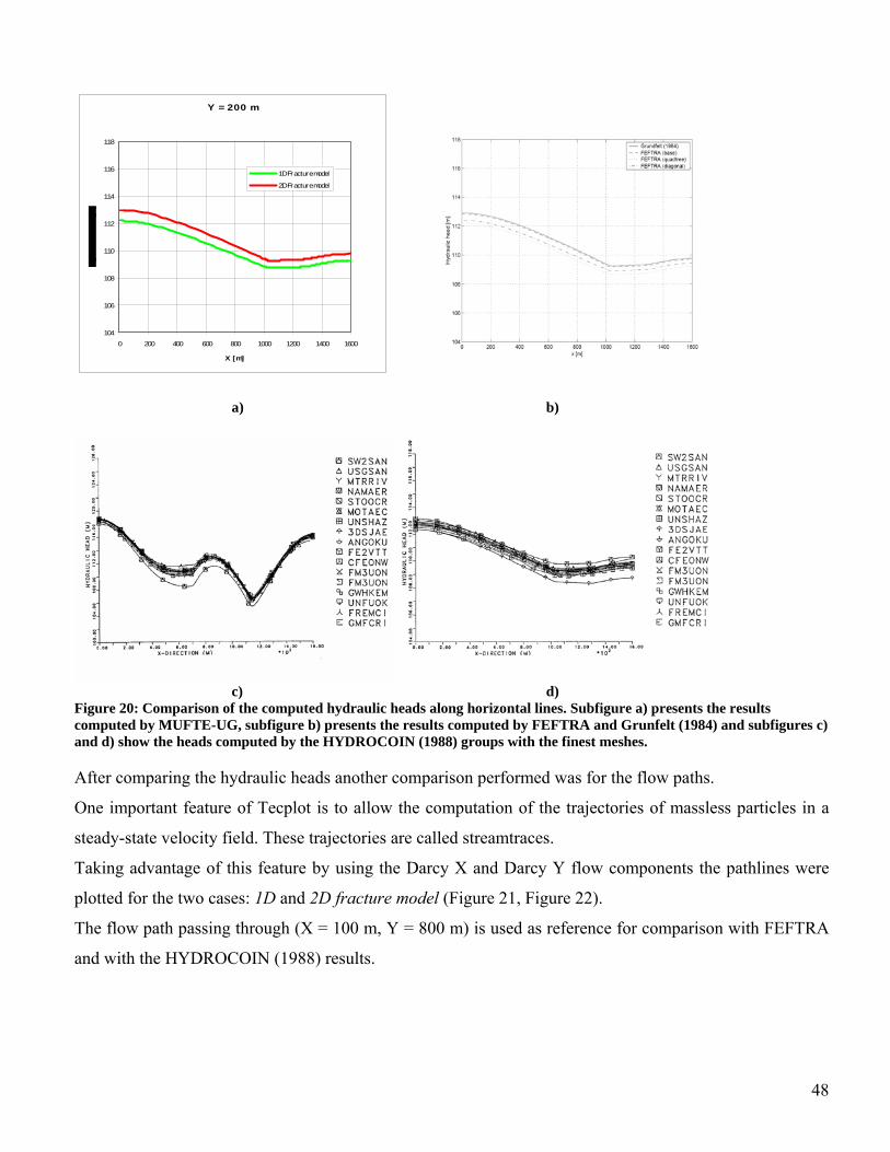
48
Y = 200 m
104
106
108
110
112
114
116
118
0 200 400 600 800 1000 1200 1400 1600
X [m]
1D Fracture model
2D Fracture model
a) b)
c) d) Figure 20: Comparison of the computed hydraulic heads along horizontal lines. Subfigure a) presents the results computed by MUFTE-UG, subfigure b) presents the results computed by FEFTRA and Grunfelt (1984) and subfigures c) and d) show the heads computed by the HYDROCOIN (1988) groups with the finest meshes.
After comparing the hydraulic heads another comparison performed was for the flow paths.
One important feature of Tecplot is to allow the computation of the trajectories of massless particles in a
steady-state velocity field. These trajectories are called streamtraces.
Taking advantage of this feature by using the Darcy X and Darcy Y flow components the pathlines were
plotted for the two cases: 1D and 2D fracture model (Figure 21, Figure 22).
The flow path passing through (X = 100 m, Y = 800 m) is used as reference for comparison with FEFTRA
and with the HYDROCOIN (1988) results.

49
a) b) Figure 21: Path lines (streamtraces) in the modeled region of a) 1D fracture model ; b) 2D fracture model
a) b) Figure 22: Path lines passing through the point (X=100 m; Y = 800 m) for a) 1D fracture model b) 2D fracture model
Figure 23: Path lines passing through (X = 100, Y=800) for the 1D and 2D fracture model computed with MUFTE-UG
and for quadtree, diagonal and base cases computed with FEFTRA

50
Figure 24: Flow path by the HYDROCOIN (1988) groups
The comparison of MUFTE to FEFTRA results and to the analytical, semianalytical and/or other numerical
solutions proves the capability of MUFTE to simulate such problems.
5.1.8 Grid Convergence Test Simulations with too coarse grids result in numerical diffusion but on the other hand simulations with very
fine grids require longer computational time. Therefore, a grid convergence test is necessary to decide
which grid size is acceptable considering the amount of numerical diffusion.
Several grid discretizations were tested. The discretizations are listed in Table 4 for 1D fracture model and
Table 5 for 2D fracture model together with the time necessary for generating them, their number of
vertexes, edges and elements, and the corresponding refinement.
The last columns of the table exhibit the time required to run the MUFTE-UG with the respective geometry
discretization.
To run these simulations a Pentium III (Coppermine) processor with 1 GHz and a 512 MB RAM memory
were used.
The real time – is the elapsed time from the beginning to the end of the program.
However, the CPU time is divided into user and sys. The user value is the time used by the program itself
and any library subroutines it calls. The sys value is the time used by system calls invoked by the program.
(directly or indirectly)
The sum of user+sys is the total direct CPU cost of executing the program. This does not include the CPU
costs of parts of the kernel that can be said to run on behalf of the program, but which do not actually run
on its thread.

51
Table 4: Discretization and computation for 1D fracture model
Computational time MUFTE [min]
real user sys Name of the ART file Matrix
Refinement [m]
Fracture Refinement
[m]
Artmesh Time [min]
Vertex
Number
Edge
Number
Face
Numbermin sec min sec min sec
q.net_1Df_500_r000 500 0 0.006667 34 79 46 0 35.1 0 1.93 0 0.826
q.net_1Df_500_r100 500 100 492 1414 923 0 35.7 0 9.641 0 0.363
q.net_1Df_500_r050 500 50 992 2896 1905 1 12.1 0 23.151 0 0.971
q.net_1Df_400_r000 400 0 0.031833 39 93 55 0 23.7 0 1.278 0 0.288
q.net_1Df_400_r100 400 100 662 1907 1246 0 39.5 0 13.207 0 0.412
q.net_1Df_400_r050 400 50 1246 3643 2398 1 3.2 0 33.37 0 0.468
q.net_1Df_300_r000 300 0 0.0315 52 130 79 0 22.8 0 1.103 0 0.231
q.net_1Df_200_r000 200 0 0.031833 69 176 108 0 23.8 0 1.224 0 0.222
q.net_1Df_100_r000 100 0 0.135667 263 730 468 0 39.3 0 4.836 0 0.36
q.net_1Df_075_r000 75 0 0.161 441 1239 799 0 43.1 0 7.606 0 0.36
q.net_1Df_050_r000 50 0 0.561167 924 2653 1730 0 54.1 0 16.844 0 0.427
q.net_1Df_050_r005 50 5 17.4968 14389 42879 28491 184
q.net_1Df_050_r003 50 3 60.5828 27294 81585 54292 1229 13.7 1207 43.801 1 26.7
q.net_1Df_045_r015 45 15 11.9823 7045 20801 13757
q.net_1Df_040_r000 40 0 0.697667 1359 3936 2578
q.net_1Df_0375_r000 37.5 0 0.748167 1514 4396 2883
q.net_1Df_037_r000 37 0 0.493167 1559 4524 2966 1 7.94 0 30.349 0 0.83
q.net_1Df_035_r000 35 0 1.03 1753 5097 3345
q.net_1Df_030_r000 30 0 1.4895 2337 6823 4487 1 31.9 0 53.742 0 0.537
q.net_1Df_025_r000 25 0 2.45367 3756 11034 7279 2 46.9 1 56.112 0 0.664
q.net_1Df_015_r000 15 0 5.56417 9354 27681 18328 9 13.6 7 56.525 0 1.57
q.net_1Df_015_r005 15 5 104.041 51799 154466 102668
q.net_1Df_010_r000 10 0 18.9512 22932 68194 45263 80 36.3 76 17.898 0 5.313
q.net_1Df_005_r000 5 0 131.733 83491 249333 165843 949 22.3 783 22.479 5 44.2
q.net_1Df_0025 2.5 0 295.375 334053 999840 665788
Table 5: Discretization and computation for 2D fracture model
Computational time MUFTE [min]
real user sys Name Matrix
Refinement Fracture
RefinementArtmesh
Time [min]
Vertex
Number
Edge
Number
Face
Numbermin sec min sec min sec
q.net_2Df1000_300_r010 300 0 0.0721667 77 199 123 0 21.587 0 0.983 0 0.239
q.net_2Df1000_200_r000 200 0 0.07483 97 254 158 0 21.154 0 1.074 0 0.231
q.net_2Df1000_200_r010 200 10 13.5972 8685 25873 17189 8 45.732 7 8.935 0 1.93
q.net_2Df1000_150_r010 150 0 0.0761667 145 390 246
q.net_2Df1000_100_r010 100 0 0.136667 283 781 499 0 22.765 0 2.145 0 0.221
q.net_2Df1000_075_r010 75 0 0.24 489 1378 890 0 19.389 0 3.327 0 0.204
q.net_2Df1000_050_r005 50 5 27.3075 17293 51563 34271
q.net_2Df1000_050_r003 50 3 91.4327 41255 123422 82168
q.net_2Df1000_050_r000 50 0 0.4365 968 2781 1814 0 24.524 0 6.081 0 0.245
q.net_2Df1000_037_r000 37 0 2.10733 1662 4825 3164 0 31.315 0 10.436 0 0.318
q.net_2Df1000_030_r000 30 0 2.26183 2433 7100 4668
q.net_2Df1000_025_r000 25 0 3.32217 3481 10210 6730 0 57.551 0 24.512 0 0.507
q.net_2Df1000_010_r000 10 0 14.6425 20896 62115 41220 11 31.343 8 24.127 0 2.779
q.net_2Df1000_005_r000 5 0 138.323 83810 250268 166459 138 31.888 102 49.333 0 44.187

52
1D fracture model Y=200
108
109
110
111
112
113
0 500 1000 1500 2000
X [m]
Hyd
raul
ic H
ead
[m]
R5
R37
R100
R200
2D fracture model Y = 200 m
108.5109
109.5110
110.5111
111.5112
112.5113
113.5
0 500 1000 1500 2000
X [m]
Hyd
raul
ic H
ead
[m]
R5
R10
R25
R30
R37
R50
R75
R100
R150
R200
1D fracture model Y=400 m
108
109
110
111
112
113
114
0 200 400 600 800 1000 1200 1400 1600 1800
X [m]
Hyd
raul
ic H
ead
[m]
R5
R37
R100
R200
2D fracture model Y = 400 m
108
109
110
111
112
113
114
0 200 400 600 800 1000 1200 1400 1600 1800
X [m]
Hyd
raul
ic H
ead
[m]
R5
R10
R25
R30
R37
R50
R75
R00
R150
R200
1D fracture model Y=600m
107
108
109
110
111
112
113
114
115
116
0 200 400 600 800 1000 1200 1400 1600 1800
X [m]
Hyd
raul
ic H
ead
[m] R5
R37
R100
R200
2D fracture model Y=600 m
107
108
109
110
111
112
113
114
115
116
0 200 400 600 800 1000 1200 1400 1600 1800
X [m]
Hyd
raul
ic H
ead
[m]
R5
R10
R25
R30
R37
R50
R75
R00
R150
R200
Figure 25: Computed hydraulic heads along horizontal lines for different grid refinements (i.e. R37) showing the grid convergence
5.1.9 Computation Time The two different fracture models computed with MUFTE-UG require different computation times as
shown in Figure 26. The 1D fracture model seems to require more time. This can be interpreted that the
box fracture algorithm utilized in the 1D fracture model requires more time than the simple box method in
2D fracture model.

53
For the case of one phase flow to apply a less dimensional fracture is not necessarily leading to an improve
in computation time.
Nevertheless, by using a less dimensional discrete fracture approach we will always need less number of
elements to represent the fracture correctly and consequently we will have a faster computation.
0
1000
2000
3000
4000
5000
6000
7000
8000
9000
0 10000 20000 30000 40000 50000 60000 70000 80000 90000
Number of nodes
Tim
e (s
econ
ds)
_
1D fracture model2D fracture model
Figure 26: Computation time for 1D and 2D fracture models using MUFTE-UG as a function of number of nodes

54
5.2 Two Fluid Phase Flow in Fractured Porous Media To demonstrate the capability of the numerical simulator MUFTE-UG we develop a two fluid phase
problem first in a 2D domain and than in a 3D domain.
5.2.1 2D Domain for Two Fluid Phase Flow in Fractured Porous Media: Hydrocoin Level 1 Case 2 (1988) Geometry
The purpose of the first numerical experiment for the two phase fracture-flow is to asses the difference
between a lower- and an equi-dimensional fracture approach. The same geometry as used in the one phase-
flow simulation is set up. (see section 5.1.2)
Similar to the one phase flow, the rock matrix is represented by 2D elements and the fracture by 1D
elements.
The boundary conditions for the two phase fracture flow in two-dimensional domain are represented in
Figure 27.
Figure 27: Boundary conditions for the two phase fluid flow problem on Hydrocoin Level 1 Case 2 geometry
The input parameters for the two media, matrix and fracture, and for the two fluid phases are given in
Table 6 and Table 7. The capillary pressure function given in the Brooks-Corey and Van Genchten
formulations is shown in Figure 28. The two phase parameters of the simulation are artificially chosen but
give a representative picture of the fracture-matrix interaction.

55
Table 6: Input parameters for the two phase fracture-flow problem in 2D domain
matrix fracture BC lambda 3.5 2
BC Pd 1000 200 Swr 0.08 0.05 Snr 0 0
VG_alpha 0.00085 0.0037 VG_n 5.65 4.7
Porosity 0.4 0.4 Abs. permeability 1.32518E-13 1.32518E-09
Table 7: The two fluid properties for the fracture-flow problem in 2D domain
Water DNAPL Density [kg/m3] 1000 1600 Dyn. Viscosity
[kg/m.s] 1.00E-03 5.70E-03
Pc-Sw
0
500
1000
1500
2000
2500
3000
0 0.1 0.2 0.3 0.4 0.5 0.6 0.7 0.8 0.9 1
Sw
Pc [P
a] _
Pc-Sw_matrix_BCPc-Sw_fracture_BCPc-Sw_matrix_VGPc-Sw_fracture_VG
Figure 28: Capillary pressure functions after Brooks Corey and Van Genuchten for Hydrocoin Level 1 Case 2 geometry
in two phase flow problem
It has to be reminded that, for all cases, the porosity of both materials (fracture and matrix) is equal to 0.4.
We compared the results obtained with different formulations of the capillary pressure (Brooks-Corey and
Van Genuchten) and in the same time we investigated the influence of the fracture absolute permeability on
the saturation front movement. The permeability values given in Table 6 are considered as initial values
and will be used to compare the results obtained with the two capillary pressure- saturation formulations.
For the 1D fracture model was conducted a simulation for comparing the influence of the fracture width on
the non-wetting saturation front.
During the simulations I vary only one parameter at the time and keep the other constant.

56
For, both the1D and 2D fracture model for two phase flow simulation I employed a mesh discretization
generated with ART (see section 4.4.3) with a constant refinement of 30 m.
The vertex-centered finite volume scheme or the box scheme was used to calculate the flow equations. For
the simulation we employ the backward Euler scheme with fixed time step size. The nonlinear equations
are solved by inexact Newton linearization. The solver used to solve the inexact Newton algorithm is the
Bi-Conjugate Gradient Stabilized solver (Bi-CGSTAB) (see Bastian [1999]).
In each Newton step a defect reduction of 1.0E-10 is prescribed and a linear defect reduction of 1.0E-05.
For the two phase flow simulation we didn’t investigate the influence of the discretization length on the
performance.
As in the case of the one-fluid phase fracture flow Hydrocoin Level 1 Case 2 (see section 5.1) this
numerical simulation was developed in several steps:
1. constructing the geometry by declaring the total number of points, edges and faces
2. discretization of the domain using ART algorithm
3. development of the numerical model in MUFTE
4. application of the numerical model MUFTE and running the simulations using MUFTE-UG
5. extraction of the saturation distribution
6. interpretation of the results
The geometry construction (step 1, 2) are the same as in the one-phase flow (see section 5.1). Step 3, the
development of the numerical model, would take too much to detail in the space of this study.
5.2.1.1 Comparison BC and VG Formulations in the 2D Fracture Model
First, we compare the Brooks-Corey (BC) and Van Genuchten (VG) formulations for capillary pressure –
saturation formulation using the parameters in Table 6. We see that there is a good agreement between the
two formulations (Figure 29). Here only the results for the 2D fracture model will be presented while for
the 1D fracture model we get the same positive agreement.
5.2.1.2 Influence of the Absolute Permeability in Fractures on the Saturation Distribution
The second numerical experiment is to assess the effect of the fracture permeability on the non-wetting
saturation front. The results are plotted for the 2D fracture model and can be seen in Figure 30.

57
T1=10x3600
T2=20x3600
T3=40x3600
T4=100x3600 a) Brooks Corey formulation b) Van Genuchten formulation
Figure 29: Comparison between the DNAPL saturation front s for 2 phase flow in the 2D fracture model for a) Brooks-Corey formulation and b) Van Genuchten formulation for time steps T1, T2, T3 and T4

58
T=10x3600
T=20x3600
T=40x3600
T=100x3600 a) b) Figure 30: Comparison between the DNAPL saturation fronts for 2 phase flow in the 2D fracture model for a constant matrix permeability Km = 1.33E-13 and tow different fracture permeabilities a) Kf1 = 1.33E-10 and b) Kf2 = 1.33E-10 for T1= 10*3600 s; T2= 20*3600 s; T3= 40*3600 s and T4= 100*3600 s;
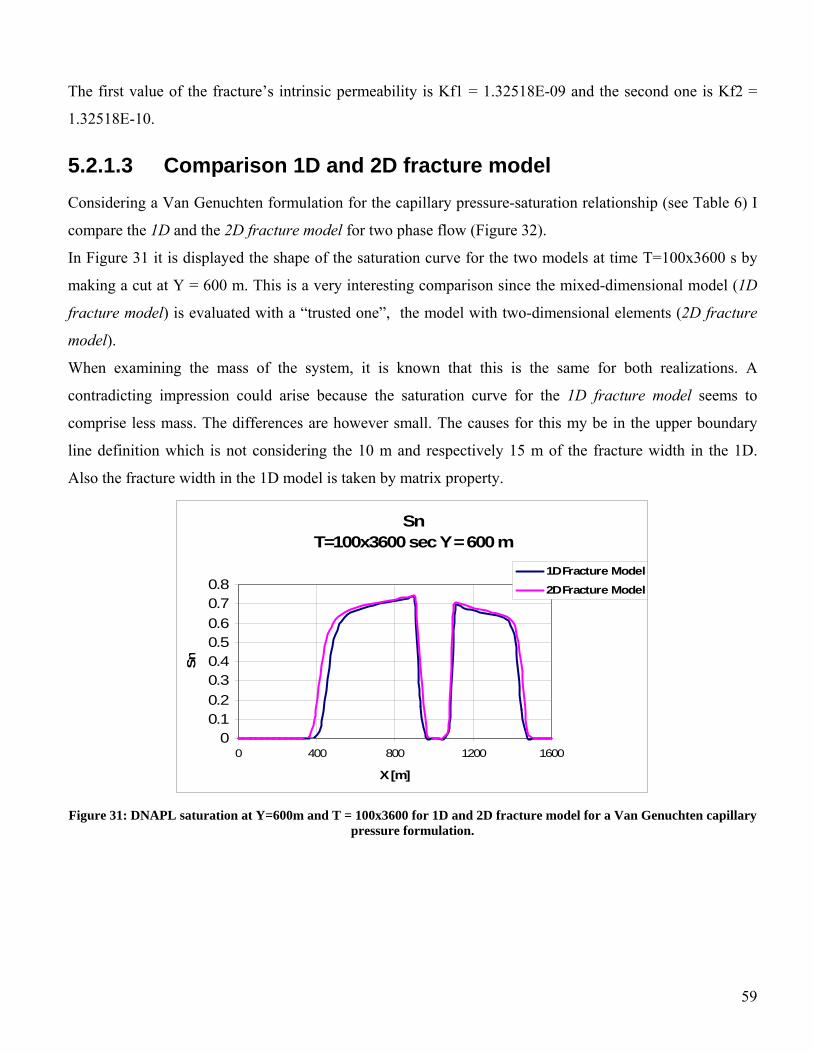
59
The first value of the fracture’s intrinsic permeability is Kf1 = 1.32518E-09 and the second one is Kf2 =
1.32518E-10.
5.2.1.3 Comparison 1D and 2D fracture model Considering a Van Genuchten formulation for the capillary pressure-saturation relationship (see Table 6) I
compare the 1D and the 2D fracture model for two phase flow (Figure 32).
In Figure 31 it is displayed the shape of the saturation curve for the two models at time T=100x3600 s by
making a cut at Y = 600 m. This is a very interesting comparison since the mixed-dimensional model (1D
fracture model) is evaluated with a “trusted one”, the model with two-dimensional elements (2D fracture
model).
When examining the mass of the system, it is known that this is the same for both realizations. A
contradicting impression could arise because the saturation curve for the 1D fracture model seems to
comprise less mass. The differences are however small. The causes for this my be in the upper boundary
line definition which is not considering the 10 m and respectively 15 m of the fracture width in the 1D.
Also the fracture width in the 1D model is taken by matrix property.
Sn T=100x3600 sec Y = 600 m
00.10.20.30.40.50.60.70.8
0 400 800 1200 1600
X [m]
Sn
1D Fracture Model2D Fracture Model
Figure 31: DNAPL saturation at Y=600m and T = 100x3600 for 1D and 2D fracture model for a Van Genuchten capillary
pressure formulation.

60
T=10x3600
T=20x3600
T=40x3600
T=100x3600 a) b) Figure 32: Saturation comparison between 1D and 2D fracture models for two phase flow using at given time steps and using a Van Genuchten capillary pressure –saturation formulation.
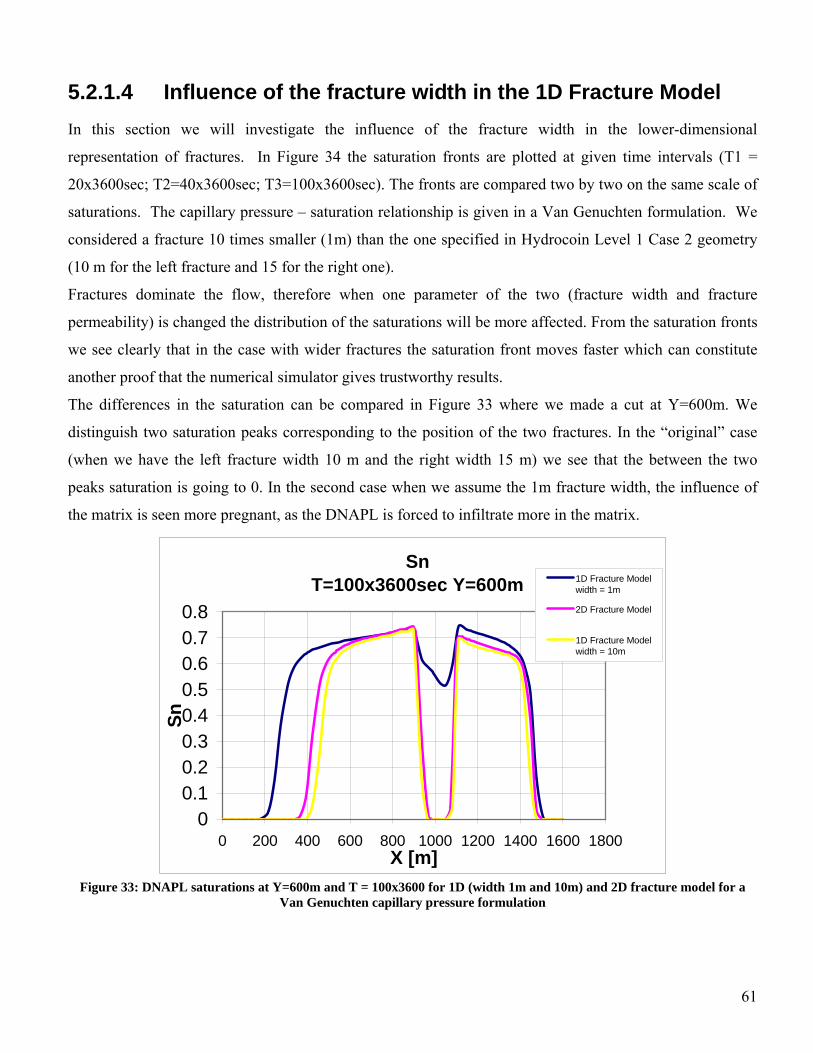
61
5.2.1.4 Influence of the fracture width in the 1D Fracture Model In this section we will investigate the influence of the fracture width in the lower-dimensional
representation of fractures. In Figure 34 the saturation fronts are plotted at given time intervals (T1 =
20x3600sec; T2=40x3600sec; T3=100x3600sec). The fronts are compared two by two on the same scale of
saturations. The capillary pressure – saturation relationship is given in a Van Genuchten formulation. We
considered a fracture 10 times smaller (1m) than the one specified in Hydrocoin Level 1 Case 2 geometry
(10 m for the left fracture and 15 for the right one).
Fractures dominate the flow, therefore when one parameter of the two (fracture width and fracture
permeability) is changed the distribution of the saturations will be more affected. From the saturation fronts
we see clearly that in the case with wider fractures the saturation front moves faster which can constitute
another proof that the numerical simulator gives trustworthy results.
The differences in the saturation can be compared in Figure 33 where we made a cut at Y=600m. We
distinguish two saturation peaks corresponding to the position of the two fractures. In the “original” case
(when we have the left fracture width 10 m and the right width 15 m) we see that the between the two
peaks saturation is going to 0. In the second case when we assume the 1m fracture width, the influence of
the matrix is seen more pregnant, as the DNAPL is forced to infiltrate more in the matrix.
Sn T=100x3600sec Y=600m
00.10.20.30.40.50.60.70.8
0 200 400 600 800 1000 1200 1400 1600 1800X [m]
Sn
1D Fracture Modelwidth = 1m
2D Fracture Model
1D Fracture Modelwidth = 10m
Figure 33: DNAPL saturations at Y=600m and T = 100x3600 for 1D (width 1m and 10m) and 2D fracture model for a
Van Genuchten capillary pressure formulation

62
T1 = 20*3600 s a) width = 1m b) width = 10m
T2 = 40*3600 s c) width = 1m d) width = 10m
T3 = 100*3600 s e) width = 1m f) width = 10m Figure 34: Saturation comparison between different fracture width in 1D fracture models at time T1 = 20x3600 sec, T2 =40 x 3600 sec, T3 =40 x 3600 sec

63
5.2.1.5 Computation Time In contrast to the one-phase fracture flow simulation where we obtained similar computation times between
the two fracture models, in the two phase fracture flow we have big differences in the computation time.
The 1D fracture model is calculated much faster. For instance the computation time in Brooks-Corey
formulation for 1D fracture model is 4.6 times faster than in 2D fracture model. Table 8: Computation time comparison for 1D and 2D fracture models in two phase flow
1Df 2Df real user sys real user sys Formulation Km
[m2] Kf
[m2] min sec min sec min sec min sec min sec min sec
BC 1.33E-13 1.33E-10 59 22.962 54 53.885 0 5.218 257 17.951 249 10.338 0 12.229VG 1.33E-13 1.33E-10 71 19.643 68 11.429 0 6.614 236 46.051 228 58.997 0 10.491
A fully coupled, fully implicit, mixed-dimensional vertex centered finite volume method for the
discretization of two-phase flow problem on unstructured grids was tested.
A comparison for a 1D fracture model showed that the differences between the lower-dimensional
discretization and the equi-dimensional discretization are small. In contrast to the equi-dimensional
discretization, the lower-dimensional discretization produces systems which are far easier to solve.

64
5.2.2 3D geometry
5.2.2.1 Definition of the problem The third numerical simulator demonstrates the applicability of a lower-dimensional fracture approach in a
three dimensional domain for multi-phase flow.
The example shown in Figure 35 was investigated in several research works concerning mesh generation
and numerics (Zielke et al. [1991], Barlag et al. [1998]). Barlag et al.[1998] analyzed the heat transport
which is characterized by poor advection in the fracture and high diffusion in the matrix.
It consists of a 3D matrix volume with an intersecting 2D fracture. The matrix is subdivided into three
blocks with different absolute permeabilities. Km1 = Km2 = 1.32518E-13 m2 and Km3 = 1.32518E-12.
The fracture’s absolute permeability is Kf = 1.23907E-07.
Figure 35: 3D geometry (Zielke et al. [1991])
The boundary conditions for the two-phase fracture flow in the three-dimensional domain are represented
in Figure 36.
The geometry is generated in ANSYS ICEM v.11.0 and exported using STAR-CD 3.2.0 solver. The way
the geometry is created and the mesh is generated is different than in ART mesh generator.

65
More characteristics of the generated geometry are specified in Table 9 (i.e. the number and name of the
constituent parts and the number of elements for each part). A finer refinement is being created along the
fracture.
Figure 36: Boundary conditions and the finite element meshes for the 3D domain
Table 9: Geometry information for 3D domain. Number of elements for the different parts of the geometry.
Part name Number of elements
1 BODY1 : 74090 2 BODY2 : 73281 3 BODY3 : 2003 4 FRACT : 9357 5 GEOM : 506 6 INFLOW : 252 7 INTERIOR : 346 8 NEUMANN : 3986 9 OUTFLOW : 28 Total elements : 163849 Total nodes : 26506
The input parameters for the two fluid phases are given in Table 10 and Table 11 and the capillary
pressure-saturation curves are represented in Figure 37.

66
Table 10: Input parameters for the two phase fracture-flow problem in 3D domain matrix 1, 2 matrix 3 fracture
lambda 2 2 3pd 500 500 200Swr 0.1 0.1 0.1Snr 0.01 0.01 0.01alpha_VG 0.00158 0.00158 0.0045n_VG 3.5 3.5 4.3porosity 0.4 0.5 0.6Kabs 1.33E-13 1.33E-12 1.24E-07
Table 11: The two fluid properties for the fracture-flow problem in 3D domain
Water DNAPL Density [kg/m3] 1000 1600 Dyn. Viscosity
[kg/m.s] 1.00E-03 5.70E-03
Pc-Sw
0
500
1000
1500
2000
2500
3000
3500
4000
4500
5000
0 0.2 0.4 0.6 0.8 1
Sw
Pc [P
a] _
Pc-Sw_matrix_BC
Pc-Sw_matrix_VG
Pc-Sw_fracture_BC
Pc-Sw_fracture_VG
Figure 37: Capillary pressure functions after Brooks Corey and Van Genuchten for 3D domain in the two phase flow
problem
The three matrix blocks have the same entry pressure and parameters that determine the capillary pressure-
saturation relationships both in Brooks-Corey and in Van Genuchten formulation.

67
5.2.2.2 Simulation Results The simulation uses the lower-dimensional centered vertex finite volume method (box fracture method).
The time discretization is the implicit backward Euler scheme. The nonlinear equations are solved by
inexact Newton linearization which is linearized by Bi-Conjugate Gradient Stabilized solver.
The computation was carried out on parallel computers of 8 nodes. Still the simulation took more than one
week. We have used the Brooks-Corey formulation for the capillary pressure saturation relationships for
the results plotted in Figure 38.
T1 = 20x3600 sec T2 = 50x3600 sec
T3 = 70x3600 sec T4 = 90x3600 sec
Figure 38: DNAPL front infiltration at different time steps for the 3D domain.

68
The DNAPL is infiltrating in the upper part and is moving along the fracture. The fracture influence is
clearly seen from the beginning of the simulation. Once the saturation front reaches the other end of the 2D
fracture another front is starting to move backwards since it cannot surpass the entry pressure of the matrix.
This is leading to problems in the convergence of the solution and consequently to high computation times.
It is obvious that the capillary forces have in this case a dominating effect.

69
6 CONCLUSIONS A small summary of what has been done is given in the following. First there were presented the main
fracture models: discrete, multi-continua and hybrid of which it has been shown that the discrete fracture
model is numerically superior for the kind of geometries we dealt with in the simulations.
Then there were introduced the mathematical models at the same time with the basic equations for single-
and the multi-phase flow in fractured porous media. Due to its advantages the phase-pressure saturation
(PPS) formulation was implemented.
After comparing the various finite element methods, the vertex centered finite volume method was picked
for solving the fully coupled fully implicit discretization. A special attention was given to the interface
conditions that represent the saturation discontinuities in lower- and equi- dimensional elements. It is worth
reminding that the vertex-centered finite volume method combines the advantages of the cell centered finite
volume discretization and the finite element discretization, and it is not only mass conservative but also can
be applied to unstructured grids.
Further on, there have been investigated three different numerical models where fractures are represented
as discrete elements. For all experiments was used the unstructured vertex-centered finite volume scheme.
We have tested and demonstrated the capability of MUFTE-UG numerical simulator to solve different
ground water problems. For the one phase simulation the results were compared to the ones obtained by
other groups in the international hydrologic code intercomparison project HYDROCOIN (1988) and to
more recent ones obtained with FEFTRA numerical simulator. The results (i.e. pressure distribution,
streamlines) show good agreement between our model and the HYDROCOIN groups. The numerical
scheme utilized by FEFTRA for solving the partial differential equations is the conventional Galerkin
technique.
One interesting aspect of this research was to compare the results obtained with the lower-dimensional
vertex centered finite volume method to the ones having the same dimensional elements in matrix and
fracture for one and two fluid phase flow in two and three dimensional domains. The results showed that
the differences between the 1D fracture model and the 2D fracture model are small and, accordingly, the
capability of MUFTE-UG to implement this model concept both in two and three dimensional domains was
demonstrated. Besides this, the lower-dimensional discretization yields systems which are far easier to
solve than those from the fully volumetric discretization approach.
In the following, the conclusions after the comparison between the lower- and equi-dimensional fracture
models, are grouped into two categories: advantages and disadvantages.
Numerically, the advantages of the lower-dimensional models are summarized as follows:
- the pre-processing is simple and does not require gridding inside the fracture

70
- avoiding small two or three-dimensional elements (depending on the case) inside the
fractures improves the conditioning of the discrete operator and also permits large time
steps.
The disadvantages of using lower dimensional elements and approach can be summarized in the following
- Though well-working in a number of applications this lower dimensional approach does not
provide local mass conservation and does not allow to follow unambiguous streamlines in and out of the
fracture. In some situations this might be a drawback. (Gebauer S. [2002])
- From the numerical simulations was seen that the equidimensional approach ends up with slightly
different results.
- A triangulation of the fractures with reasonable number of nodes may lead to long thin elements.
Though almost all the degenerate elements are not a problem from the approximation point of view (cf. e.g.
Jamet [1976]), they cause severe problems in the iterative solution of the discretized problems. For
example, classical multigrid methods usually fail for vanishing width of fractures.
In conclusion, it was demonstrated that the lower-dimensional concept is applicable for both 2D and 3D
systems and represents correctly the flow in the fractured porous media and the combination of the vertex-
centered finite volume method with the discrete fracture model provides a powerful tool to study the multi-
phase flow in fractured porous media.
Future work may include the incorporation of more complex mathematical models: multi-phase multi-
component simulations or the implementation of different discretizations.

71
References 1. Atkinson K.E.: “An Introduction to Numerical Analysis”. John Wiley &Sons, Inc. New York.
Second Edition, (1988) 2. Aziz, K. and Settari A.: “Petroleum Reservoir Simulation”, Elsevier (1979) 3. Barlag, C.: “Adaptive methods for Modeling Transport Processes in Fractured Subsurface
Systems”, 3rd International Conference on Hydroscience and Engineering, (1998) 4. Barenblatt, G.,I. and Zheltov, I.P.: “On fundamental equations of flow of homogeneous liquids in
naturally fractured rocks”, Dokl. Akad. Nauk. USSR 132 (3), 545-548, (1960) 5. Bastian P.: “Numerical computation of multi-phase flows in porous media”, Habilitation thesis,
Christian-Albrechts-Universitaet Kiel, (1999) 6. Bear, J., Tsang,C.,-H, and De Marsily, G.: 1993 “Flow and Contaminant Transport in Fractured
Rock”, Academic Press, San Diego, California, (1993) 7. Bibby, R.: “Mass transport of solutes in dual-porosity media”, Water Resources Res. 17(4), 1075-
1081, (1981) 8. Bird, R. B., Stewart, W.E., and Lightfoot E. N.: “Transport Phenomena”, John Wiley, New York,
(1960) 9. Bonnet, E., Bour O., Odling N., Main I., Berkowitz B., Davy P., and Cowie P.: “Scaling of fracture
systems in geological media”, Rev. Geophys., 39, 347-383, (2001) 10. Brooks, R.H. and Corey, A.T.,: Hydraulic properties of porous media: Hydrology Papers, Colorado
State University, (1964) 11. Brush D. and Thomson N.R. : “Fluid flow in synthetic rough-walled fractures: Navier-Stokes,
Stokes, and local cubic law simulations”; Water Resources Research, vol.39, no.4, 1085, (2003) 12. Chavent, G. and Jaffré J. : “Mathematical Models and Finite Elements for Reservoir Simulation”,
North-Holland, (1978) 13. Duijn C.J. van, Molenaar J., De Neef M.J. : “The effect of capillary forces on immiscibe two-phase
flow in heterogeneous porous media”; Trans. Porous Media 21, 71-93, (1995) 14. Ersland B.G. et al.: “Numerical methods for flow in a porous medium with internal boundaries”
Computational Geosciences 2, p217-240, (1998) 15. Fuchs, A.: “Optimierte Delauney-Triangulation zur Vernetzung getrimmter NURBs-Körper,
Dissertation”, Shker Verlag, (1999) 16. Gebauer S., Neunhäuserer L. , Kornhuber R., Ochs S., Hinkelmann R., Helmig R.:
“Equidimensional modeling of flow and transport processes in fractured porous systems” , International Conference on Computational Methods in Water Resources, Delft, (2002)
17. Geiger S., Niessner J., Matthäi S., Helmig R.: “Black-Oil Simulations for Three-Component Three-Phase Flow in Fractured Porous Media”; SPE International, (2007)
18. Genuchten, M.Th. van,: “ A closed-form equation for predicting the hydraulic conductivity of unsaturated soils”. Soil.Sci.Soc.Am. J44:892-898, (1980)
19. Helmig R.: “Multiphase flow and transport processes in the subsurface – a contribution to the modeling of Hydrosystems”, Berlin: Springer-Verlag, (1997)
20. Hinkelmann R.: “Efficient numerical methods and information-processing techniques in environment water”. Institut für Wasserbau – Universität Stuttgart, (2003)
21. Hornung, U., editor: “Homogenization and Porous Media, volume 6 of Interdisciplinary Applied Mathematics”. Springer-Verlag, Berlin, Heidelberg, New York, (1997)
22. Hoteit H., Firoozabadi A., “Multicomponent fluid flow by discontinuous Galerkin and mixed methods in unfractured and fractured media”
23. Huyakorn, P.,S., Lester, B.H. and Mercer, J.,W.: “An efficient finite element technique for modeling transport in fractured porous media, 1, single species transport”, Water Resources Res. 19(3), 841-854, (1983)

72
24. Jamet P.: “Estimation d’erreur pour des elements finis droits Presque degeneres”; R.A.I.R.O., Serie Analyse Numerique, 10, No.3, p.43-61, (1976)
25. Juanes R., Samper J., Molinero J.: “A general and efficient formulation of fractures and boundary conditions in the finite element method”, International Journal for Numerical Methods in Engineering; 54:1751-1774, (2002)
26. Karimi-Fard M., Durlofsky L.J., Aziz K.: “An Efficient Discrete-Fracture Model Applicable for General-Purpose Reservoir Simulators” SPE J. , 9, 227-236, (2004)
27. Karimi-Fard M., Firoozabadi A.: “Numerical Simulation of Water Injection in 2D Fractured Media Using Discrete-Fracture Model” (2001)
28. Löfman, Jari, Keto, Vesa & Mészáros, Ferenc : “FEFTRATM. Verification. Espoo 2007. VTT” Tiedotteita Research Notes 2385. 103 p. + app. 4 p, (2007)
29. Molenar J.: “Multigrid methods for fully implicit oil reservoir simulation”, In Proceedings Copper Mountain Conference on Multigrid Methods (1995)
30. Niessner et al.: “Interface condition and linearization schemes in the Newton iterations for two-phase flow in heterogeneous porous media”, Advances in Water Resources 28, 671-687, (2005)
31. Oian E. , Berg S. S.: “Hierarchical approach for simulating fluid flow in normal fault zones”, Petroleum Geoscience, Vol.13, No.1, pp.25-35, (2007)
32. Peaceman, D.W. : “Fundamentals of Numerical Reservoir Simulation”, Elsevier, (1977) 33. Reichenberger V., Jakobs H., Bastian P., Helmig R., Niessner J., “Complex Gas-Water Processes in
Discrete Fracture-Matrix Systems: Up-scaling, Mass-Conservative Discretization and Efficient Multilevel Solution”; Institut für Wasserbau, Universität Stuttgart, Heft 130, (2004)
34. Reichenberger V., Jakobs H., Bastian P., Helmig R.,: A mixed-dimensional finite volume method for two-phase flow in fractured porous media; Advances in Water Resources 29, 1020-1036, (2006)
35. Royer P. ,Auriault J.-L., Lewandowska J., Serres C. “Continuum Modeling of Contaminant Transport in Fractured Porous Media”; Kluwer Academic Plubishers (2002)
36. Sahimi, M., “Flow and Transport in Porous Media and Fractured Rock: From Classical Methods to Modern Approaches”, VCH, Weinheim, (1995)
37. Singhal B.B.S. and Gupta R. P. : “Applied Hydrogeology of Fractured Rocks”. Kluwer Academic Publishers, Dordrecht, Boston, London, (1999b)
38. Wu Y.-S. and Pruess, K., “Numerical simulation of non-isothermal multiphase tracer transport in heterogeneous fractured porous media”. Advances in Water Resources, 23:699-723, (2000)
39. Zielke, W., Helmig, R., Kröhn, K.-P., Shao,H., Wollrath, J.: “Discret Modelling of Transport Processes in Fractured Porous Rock” in Wittke (editor): International Congress on Rock Mechanics, 57-60, International Society for Rock Mechanics, (1991)

73
APPENDIX
Structure of the Application Example for one phase flow in 1D fracture model (SIM_1D_frac)
The development in MUFTE of numerical simulation of one-phase flow for the HYDROCOIN (1998)
geometry assuming fractures as one dimensional elements is presented here. The application name is k1
and the folder name containing the application has been given “SIM_1D_frac”. This chapter contains the
overview of all files of the application problem k1.
The application directory SIM_1D_frac contains the following files:
• C-file: initall.c • C-file: k1_fflow.c • C-file: k1_ftransp.c • C-file: q_fbvp.c • Script-file: k1_ftitrp.scr • defaults • Makefile
• Script file k1_ftitrp.scr The interaction between MUFTE application and the UG-library is being done by the scrip-file. All the
commands used in the script file are defined in ug/ui/commands.c. The fracture-matrix domain is
previously discretized using ART and the files q.bnd and q.net provide the domain and the mesh
information.
The script-file opens with the logon command which controls the output to a log-file. In the same way the
file ends with a logoff command. ########################################################
#open log file
########################################################
logon k1_ftitrp.log;
Afterwards are defined the main parameters of the simulation. ########################################################
# some constants
########################################################
BASELEVEL = 0; # start from this level
MAXLEVEL = 0; # finest level
DOGLS = 0; # plot matrix;
DOGRAPHICS = 1; # plot results
DOFILMS = 1; # do output either tecplot or dataxplorer film
DOTECPLOT = 1; # do tecplot film
DODX = 0;
TECPLOTINC = 10; # no of time-steps per frame
fsteps = 350; # total number of time steps for flow (>1!)
tsteps = 10; # total number of time steps for transport
DTSTART = 10; # initial time step

74
DT = 10; #
END = 100*86400.0; # end of simulation time
DTMIN = 1; # smallest time step
########################################################
# create coarse mesh
########################################################
readartbnd q.bnd;
new fractk1 $b qBVP $f FlowTIFormat $h @HEAP;
readartnet q.net;
refreshon;
fixcoarsegrid;
@gw;
The flow and transport variables in the single-phase problem as well as the values of the boundary
conditions are defined in the script-file. ########################################################
# initialize input data
########################################################
# BVP values
source = 6.0E-08; # [kg/sm^2]
time1 = 30;
thickness = 1.0; # Set to 1.0 for 3D applications
fract1_width = 10.0;
fract2_width = 15.0;
fract1_prop = -1.0;
fract2_prop = -2.0;
k_x_1 = 1.32518E-15; # [m^2] matrix permeability
k_y_1 = 1.32518E-15; # [m^2]
k_z_1 = 1.32518E-15; # [m^2]
fract1_k_0 = 1.32518E-12; # [m^2] fracture 1 permeability
fract2_k_0 = 1.32518E-13; # [m^2] fracture 2 permeability
flow_visc = 0.0013; # dynamic viscosity!!! (water)
flow_dens = 1000.0; # water
dens_mode = 0; # 0=incompressible, 1=compressible
# For dens_mode = 1: If not air, change
stor_coeff = 1.0e-4; # only needed for dens_mode = 1
fract_stor_coeff = 1.0e-4; # only needed for dens_mode = 1
mat_poros = 0.13; # used for transport and dens_mode = 1
fract1_poros = 0.30; # used for transport and dens_mode = 1
fract2_poros = 0.30; # used for transport and dens_mode = 1
# transport values
tracer_dens = 1.0; # If 1 - same as fluid. Output conc [kg(subst.)/m^3(mixture)]
mat_disp_l = 1.0e-9; # alpha_l (minimized)
mat_disp_t = 1.0e-9; # alpha_t (minimized)
fract1_disp_l = 0.0;
fract2_disp_l = 0.0;
mol_diff_fract = 1.0e-9; # Deff (minimized)
mol_diff_mat = 1.0e-9; # Deff (minimized)

75
The values for several parameters describing the fluid porous-medium properties or the interaction between
fluid and matrix are set in the following. The functions will be later described in the c-files.
For steady state: ########################################################
# set up steady state discretization scheme
########################################################
npcreate fk1f $c fk1f;
npinit fk1f $p pressure;
npcreate fbf $c fbf;
npinit fbf $A MAT $x pressure $b rhs $P fk1f;
########################################################
# set up steady state flow solver
########################################################
npcreate ilu $c ilu;
npinit ilu $damp 1.0;
npcreate base $c ex;
npinit base;
npcreate basesolver $c ls;
npinit basesolver $red 1.0E-4 $m 50 $I base $display no;
npcreate transfer $c transfer;
npinit transfer $x pressure $S 2.0;
npcreate lmgc $c lmgc;
npinit lmgc $S ilu ilu basesolver $T transfer $n1 2 $n2 2 $g 1;
npcreate mgs $c bcgs;
npinit mgs $A MAT $x pressure $b rhs $m 25 $red 1.0E-6
$abslimit 1.0E-15 $I lmgc $display full;
For transient flow: ########################################################
# set up transient flow discretization scheme
########################################################
npcreate fbfti $c fbfti;
npinit fbfti $FP fk1f;
########################################################
# set up transient flow solver
########################################################
#grid transfer numproc
npcreate fti_transfer $c transfer;
npinit fti_transfer $x pressure $S 2.0;
#linear solver and iteration numprocs
npcreate fti_smooth $c sgs;
npinit fti_smooth $damp 1.0;
npcreate fti_base $c ex;
npinit fti_base;

76
npcreate fti_basesolver $c ls;
npinit fti_basesolver $abslimit 1.0E-15 $red 0.001 $m 10 $I fti_base;
npcreate fti_lmgc $c lmgc;
npinit fti_lmgc $S fti_smooth fti_smooth fti_basesolver $T fti_transfer
$n1 2 $n2 2 $g 1 $b 0;
npcreate fti_mgs $c bcgs;
npinit fti_mgs $abslimit 1.0E-15 $m 40 $I fti_lmgc $display full;
# nonlinear solver numproc to be used by time solver
npcreate fti_newton $c newton;
npinit fti_newton $abslimit 1.0E-8 $red 1.0E-10 $T fti_transfer $S fti_mgs
$rhoreass 0.8 $lsteps 6 $maxit 50 $line 1 $linrate 0
$lambda 1.0 $linminred 1.0E-5 $divfac 1.0E100 $display red;
# the time solver
npcreate fti_ts $c bdf;
npinit fti_ts $y pressure $A fbfti $S fti_newton $T fti_transfer
$baselevel 0 $order 1 $predictorder 0 $nested 0
$dtstart @DT $dtmin @DTMIN $dtmax @DT $dtscale 1.0 $rhogood 0.001;
########################################################
# set up transport discretization scheme
########################################################
npcreate fk1t $c fk1t;
npinit fk1t;
npcreate fbt $c fbt;
npinit fbt $FP fk1f $TP fk1t $alpha 1.0 $so 0 $calc 0;
########################################################
# set up transport solver
########################################################
#grid transfer numproc
npcreate t_transfer $c transfer;
npinit t_transfer $x sol $S 2.0;
#linear solver and iteration numprocs
npcreate t_smooth $c sgs;
npinit t_smooth $damp 1.0;
npcreate t_base $c ex;
npinit t_base;
npcreate t_basesolver $c ls;
npinit t_basesolver $abslimit 1.0E-15 $red 0.001 $m 10 $I t_base;
npcreate t_lmgc $c lmgc;
npinit t_lmgc $S t_smooth t_smooth t_basesolver $T t_transfer $n1 2 $n2 2
$g 1 $b 0;
npcreate t_mgs $c bcgs;
npinit t_mgs $abslimit 1.0E-15 $m 40 $I t_lmgc $display full;
# nonlinear solver numproc to be used by time solver
npcreate newton $c newton;
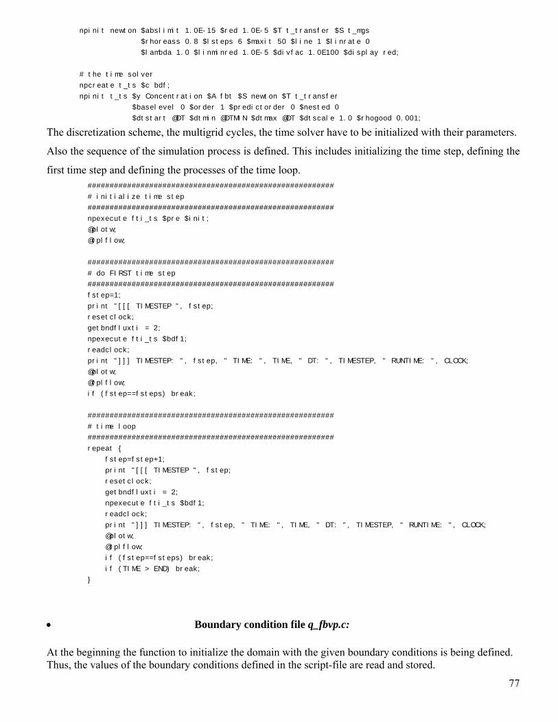
77
npinit newton $abslimit 1.0E-15 $red 1.0E-5 $T t_transfer $S t_mgs
$rhoreass 0.8 $lsteps 6 $maxit 50 $line 1 $linrate 0
$lambda 1.0 $linminred 1.0E-5 $divfac 1.0E100 $display red;
# the time solver
npcreate t_ts $c bdf;
npinit t_ts $y Concentration $A fbt $S newton $T t_transfer
$baselevel 0 $order 1 $predictorder 0 $nested 0
$dtstart @DT $dtmin @DTMIN $dtmax @DT $dtscale 1.0 $rhogood 0.001;
The discretization scheme, the multigrid cycles, the time solver have to be initialized with their parameters.
Also the sequence of the simulation process is defined. This includes initializing the time step, defining the
first time step and defining the processes of the time loop. ########################################################
# initialize time step
########################################################
npexecute fti_ts $pre $init;
@plotw;
@tplflow;
########################################################
# do FIRST time step
########################################################
fstep=1;
print "[[[ TIMESTEP ", fstep;
resetclock;
getbndfluxti = 2;
npexecute fti_ts $bdf1;
readclock;
print "]]] TIMESTEP: ", fstep, " TIME: ", TIME, " DT: ", TIMESTEP, " RUNTIME: ", CLOCK;
@plotw;
@tplflow;
if (fstep==fsteps) break;
########################################################
# time loop
########################################################
repeat
fstep=fstep+1;
print "[[[ TIMESTEP ", fstep;
resetclock;
getbndfluxti = 2;
npexecute fti_ts $bdf1;
readclock;
print "]]] TIMESTEP: ", fstep, " TIME: ", TIME, " DT: ", TIMESTEP, " RUNTIME: ", CLOCK;
@plotw;
@tplflow;
if (fstep==fsteps) break;
if (TIME > END) break;
• Boundary condition file q_fbvp.c: At the beginning the function to initialize the domain with the given boundary conditions is being defined. Thus, the values of the boundary conditions defined in the script-file are read and stored.

78
/**************************************************************************/
/* read in constant boundary conditions and more*/
/**************************************************************************/
static DOUBLE
source,time1,fract1_width,fract1_prop,fract2_width,fract2_prop;
static INT FractK1ProblemConfig (INT argc, char **argv)
/* read a string variable */
GetStringValueDouble("upper_p",&upper_p);
GetStringValueDouble("lower_p",&lower_p);
GetStringValueDouble("source",&source);
GetStringValueDouble("time1",&time1);
GetStringValueDouble("fract1_width",&fract1_width);
GetStringValueDouble("fract1_prop",&fract1_prop);
GetStringValueDouble("fract2_width",&fract2_width);
GetStringValueDouble("fract2_prop",&fract2_prop);
return(0);
The boundary conditions are defined in the following. For the North Boundary the head is defined as
h(x,y) = y
so two functions have to be defined, respectively for the descending and ascending slope. The two
functions are called K1ProblemInBoundary1 and K1ProblemInBoundary2. static INT K1ProblemInBoundary1 (void *segdata, void *conddata, DOUBLE *in, DOUBLE *outValues, INT
*bndType)
DOUBLE time;
DOUBLE lambda;
lambda = in[0];
time = in[IN_T];
bndType[OUT_BNDTYP_fit] = DIRICHLET;
bndType[OUT_BNDTYP_fti] = DIRICHLET;
outValues[OUT_BNDVAL_fit] = 9.81*1000*(150-lambda*50);
outValues[OUT_BNDVAL_fti] = 9.81*1000*(150-lambda*50);
bndType[OUT_BNDTYP_trp] = NEUMANN;
outValues[OUT_BNDVAL_trp] = source;
if (time <= time1)
outValues[OUT_BNDVAL_trp] = source;
else
outValues[OUT_BNDVAL_trp] = 0.0;
return(0);
static INT K1ProblemInBoundary2 (void *segdata, void *conddata, DOUBLE *in, DOUBLE *outValues, INT
*bndType)

79
DOUBLE time;
DOUBLE lambda;
lambda = in[0];
time = in[IN_T];
bndType[OUT_BNDTYP_fit] = DIRICHLET;
bndType[OUT_BNDTYP_fti] = DIRICHLET;
outValues[OUT_BNDVAL_fit] = 9.81*1000*(lambda*50+100);
outValues[OUT_BNDVAL_fti] = 9.81*1000*(lambda*50+100);
bndType[OUT_BNDTYP_trp] = NEUMANN;
outValues[OUT_BNDVAL_trp] = source;
if (time <= time1)
outValues[OUT_BNDVAL_trp] = source;
else
outValues[OUT_BNDVAL_trp] = 0.0;
return(0);