numerical integration - physicsntg/6810/readings/hjorth-jensen... · chapter 5 numerical...
TRANSCRIPT

Chapter 5
Numerical Integration
Abstract In this chapter we discuss some of the classical methods for integrating a func-tion. The methods we discuss are the trapezoidal, rectangular and Simpson’s rule for equallyspaced abscissas and integration approaches based on Gaussian quadrature. The latter aremore suitable for the case where the abscissas are not equally spaced. The emphasis is onmethods for evaluating few-dimensional (typically up to four dimensions) integrals. In chapter11 we show how Monte Carlo methods can be used to compute multi-dimensional integrals.We discuss also how to compute singular integrals. We end this chapter with an extensive dis-cussion on MPI and parallel computing. The examples focus on parallelization of algorithmsfor computing integrals.
5.1 Newton-Cotes Quadrature
The integral
I =! b
af (x)dx (5.1)
has a very simple meaning. If we consider Fig. 5.1 the integral I simply represents the areaenscribed by the function f (x) starting from x= a and ending at x= b. Two main methods willbe discussed below, the first one being based on equal (or allowing for slight modifications)steps and the other on more adaptive steps, namely so-called Gaussian quadrature methods.Both main methods encompass a plethora of approximations and only some of them will bediscussed here.
In considering equal step methods, our basic approach is that of approximating a functionf (x) with a polynomial of at most degree N! 1, given N integration points. If our polynomialis of degree 1, the function will be approximated with f (x)" a0+a1x. The algorithm for theseintegration methods is rather simple, and the number of approximations perhaps unlimited!
• Choose a step size
h=b! aN
where N is the number of steps and a and b the lower and upper limits of integration.• With a given step length we rewrite the integral as
! b
af (x)dx=
! a+h
af (x)dx+
! a+2h
a+hf (x)dx+ . . .
! b
b!hf (x)dx.
109

110 5 Numerical Integration
!
f (x)
x
"
a a+h a+2h a+3h bFig. 5.1 The area enscribed by the function f (x) starting from x= a to x= b. It is subdivided in several smallerareas whose evaluation is to be approximated by the techniques discussed in the text. The areas under thecurve can for example be approximated by rectangular boxes or trapezoids.
• The strategy then is to find a reliable polynomial approximation for f (x) in the variousintervals. Choosing a given approximation for f (x), we obtain a specific approximation tothe integral.
• With this approximation to f (x) we perform the integration by computing the integrals overall subintervals.
Such a small measure may seemingly allow for the derivation of various integrals. To see this,we rewrite the integral as
! b
af (x)dx =
! a+2h
af (x)dx+
! a+4h
a+2hf (x)dx+ . . .
! b
b!2hf (x)dx.
One possible strategy then is to find a reliable polynomial expansion for f (x) in the smallersubintervals. Consider for example evaluating
! a+2h
af (x)dx,
which we rewrite as ! a+2h
af (x)dx =
! x0+h
x0!hf (x)dx. (5.2)
We have chosen a midpoint x0 and have defined x0 = a+ h. Using Lagrange’s interpolationformula from Eq. (3.9), an equation we restate here,
5.1 Newton-Cotes Quadrature 111
PN(x) =N
∑i=0∏k #=i
x! xkxi! xk
yi,
we could attempt to approximate the function f (x) with a first-order polynomial in x in thetwo sub-intervals x $ [x0! h,x0] and x $ [x0,x0+ h]. A first order polynomial means simply thatwe have for say the interval x $ [x0,x0+ h]
f (x) " P1(x) =x! x0
(x0+ h)! x0f (x0+ h)+
x! (x0+ h)x0! (x0+ h)
f (x0),
and for the interval x $ [x0! h,x0]
f (x) " P1(x) =x! (x0! h)x0! (x0! h)
f (x0)+x! x0
(x0! h)! x0f (x0! h).
Having performed this subdivision and polynomial approximation, one from x0! h to x0 andthe other from x0 to x0+ h,
! a+2h
af (x)dx =
! x0
x0!hf (x)dx+
! x0+h
x0f (x)dx,
we can easily calculate for example the second integral as
! x0+h
x0f (x)dx "
! x0+h
x0
"x! x0
(x0+ h)! x0f (x0+ h)+
x! (x0+ h)x0! (x0+ h)
f (x0)#dx,
which can be simplified to
! x0+h
x0f (x)dx"
! x0+h
x0
"x! x0h
f (x0+ h)!x! (x0+ h)
hf (x0)
#dx,
resulting in ! x0+h
x0f (x)dx=
h2( f (x0+ h)+ f (x0))+O(h3).
Here we added the error made in approximating our integral with a polynomial of degree 1.The other integral gives
! x0
x0!hf (x)dx =
h2( f (x0)+ f (x0! h))+O(h3),
and adding up we obtain
! x0+h
x0!hf (x)dx =
h2( f (x0+ h)+ 2 f (x0)+ f (x0! h))+O(h3), (5.3)
which is the well-known trapezoidal rule. Concerning the error in the approximation made,O(h3) = O((b! a)3/N3), you should note the following. This is the local error! Since we aresplitting the integral from a to b in N pieces, we will have to perform approximately N suchoperations. This means that the global error goes like " O(h2). To see that, we use the trape-zoidal rule to compute the integral of Eq. (5.1),
I =! b
af (x)dx= h( f (a)/2+ f (a+ h)+ f (a+ 2h)+ · · ·+ f (b! h)+ fb/2) , (5.4)
with a global error which goes like O(h2).
112 5 Numerical Integration
Hereafter we use the shorthand notations f!h = f (x0! h), f0 = f (x0) and fh = f (x0+ h). Thecorrect mathematical expression for the local error for the trapezoidal rule is
! b
af (x)dx!
b! a2
[ f (a)+ f (b)] =!h3
12f (2)(ξ ),
and the global error reads
! b
af (x)dx!Th( f ) =!
b! a12
h2 f (2)(ξ ),
where Th is the trapezoidal result and ξ $ [a,b].The trapezoidal rule is easy to implement numerically through the following simple algo-
rithm
• Choose the number of mesh points and fix the step.• calculate f (a) and f (b) and multiply with h/2• Perform a loop over n = 1 to n! 1 ( f (a) and f (b) are known) and sum up the terms
f (a+ h)+ f (a+ 2h)+ f (a+ 3h)+ · · ·+ f (b! h). Each step in the loop corresponds to agiven value a+ nh.
• Multiply the final result by h and add h f (a)/2 and h f (b)/2.
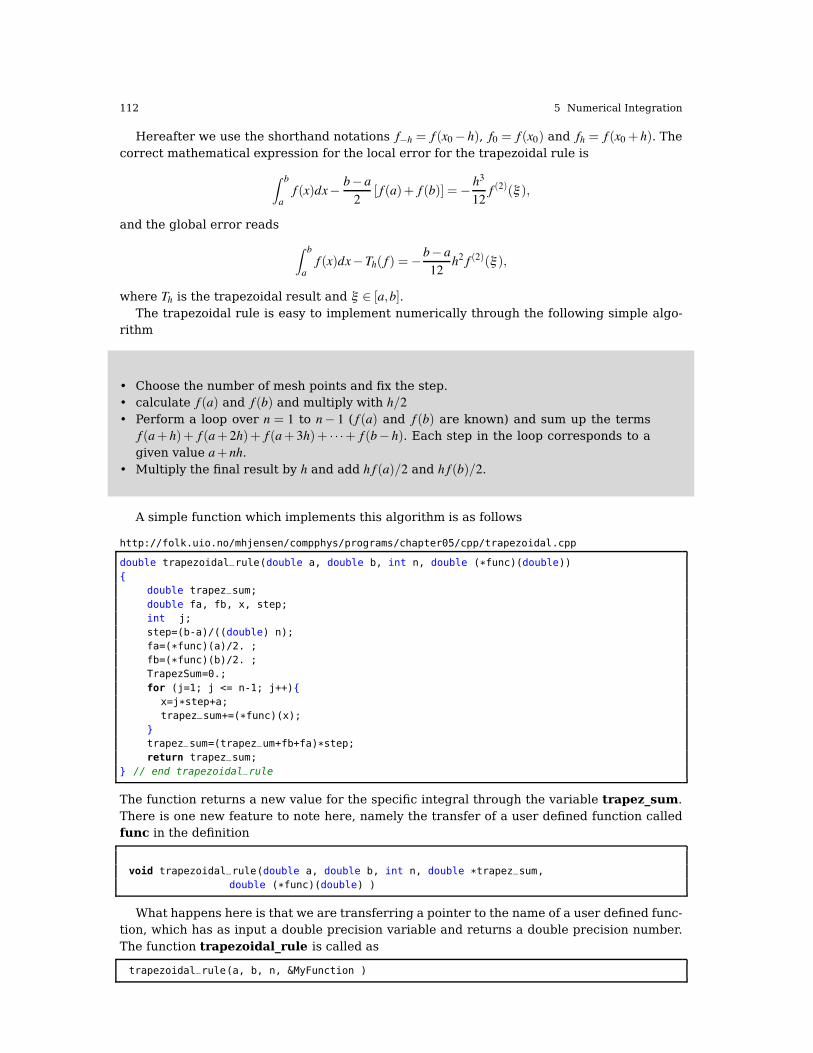
A simple function which implements this algorithm is as follows
http://folk.uio.no/mhjensen/compphys/programs/chapter05/cpp/trapezoidal.cpp
double trapezoidal_rule(double a, double b, int n, double (*func)(double)){
double trapez_sum;
double fa, fb, x, step;int j;step=(b-a)/((double) n);fa=(*func)(a)/2. ;fb=(*func)(b)/2. ;TrapezSum=0.;
for (j=1; j <= n-1; j++){x=j*step+a;trapez_sum+=(*func)(x);
}trapez_sum=(trapez_um+fb+fa)*step;return trapez_sum;
} // end trapezoidal_rule
The function returns a new value for the specific integral through the variable trapez_sum.There is one new feature to note here, namely the transfer of a user defined function calledfunc in the definition
void trapezoidal_rule(double a, double b, int n, double *trapez_sum,double (*func)(double) )
What happens here is that we are transferring a pointer to the name of a user defined func-tion, which has as input a double precision variable and returns a double precision number.The function trapezoidal_rule is called as
trapezoidal_rule(a, b, n, &MyFunction )

5.1 Newton-Cotes Quadrature 113
in the calling function. We note that a, b and n are called by value, while trapez_sum andthe user defined function MyFunction are called by reference.
The name trapezoidal rule follows from the simple fact that it has a simple geometricalinterpretation, it corresponds namely to summing up a series of trapezoids, which are theapproximations to the area below the curve f (x).
Another very simple approach is the so-called midpoint or rectangle method. In this casethe integration area is split in a given number of rectangles with length h and height givenby the mid-point value of the function. This gives the following simple rule for approximatingan integral
I =! b
af (x)dx " h
N
∑i=1
f (xi!1/2), (5.5)
where f (xi!1/2) is the midpoint value of f for a given rectangle. We will discuss its truncationerror below. It is easy to implement this algorithm, as shown here
http://folk.uio.no/mhjensen/compphys/programs/chapter05/cpp/rectangle.cpp
double rectangle_rule(double a, double b, int n, double (*func)(double)){
double rectangle_sum;double fa, fb, x, step;int j;
step=(b-a)/((double) n);rectangle_sum=0.;for (j = 0; j <= n; j++){
x = (j+0.5)*step+; // midpoint of a given rectangle
rectangle_sum+=(*func)(x); // add value of function.
}
rectangle_sum *= step; // multiply with step length.
return rectangle_sum;} // end rectangle_rule
The correct mathematical expression for the local error for the rectangular rule Ri(h) forelement i is ! h
!hf (x)dx!Ri(h) =!
h3
24f (2)(ξ ),
and the global error reads
! b
af (x)dx!Rh( f ) =!
b! a24
h2 f (2)(ξ ),
where Rh is the result obtained with rectangular rule and ξ $ [a,b].Instead of using the above first-order polynomials approximations for f , we attempt at
using a second-order polynomials. In this case we need three points in order to define asecond-order polynomial approximation
f (x) " P2(x) = a0+ a1x+ a2x2.
Using again Lagrange’s interpolation formula we have
P2(x) =(x! x0)(x! x1)(x2! x0)(x2! x1)
y2+(x! x0)(x! x2)(x1! x0)(x1! x2)
y1+(x! x1)(x! x2)(x0! x1)(x0! x2)
y0.
Inserting this formula in the integral of Eq. (5.2) we obtain
! +h
!hf (x)dx=
h3( fh+ 4 f0+ f!h)+O(h5),

114 5 Numerical Integration
which is Simpson’s rule. Note that the improved accuracy in the evaluation of the deriva-tives gives a better error approximation, O(h5) vs. O(h3) . But this is again the local errorapproximation. Using Simpson’s rule we can easily compute the integral of Eq. (5.1) to be
I =! b
af (x)dx =
h3( f (a)+ 4 f (a+ h)+ 2 f (a+ 2h)+ · · ·+ 4 f (b! h)+ fb) , (5.6)
with a global error which goes like O(h4). More formal expressions for the local and globalerrors are for the local error
! b
af (x)dx!
b! a6 [ f (a)+ 4 f ((a+ b)/2)+ f (b)] =!
h5
90 f(4)(ξ ),
and for the global error ! b
af (x)dx! Sh( f ) =!
b! a180
h4 f (4)(ξ ).
with ξ $ [a,b] and Sh the results obtained with Simpson’s method. The method can easily beimplemented numerically through the following simple algorithm
• Choose the number of mesh points and fix the step.• calculate f (a) and f (b)• Perform a loop over n = 1 to n! 1 ( f (a) and f (b) are known) and sum up the terms4 f (a+ h)+ 2 f (a+ 2h)+ 4 f (a+ 3h)+ · · ·+ 4 f (b! h). Each step in the loop correspondsto a given value a+ nh. Odd values of n give 4 as factor while even values yield 2 asfactor.
• Multiply the final result by h3 .
In more general terms, what we have done here is to approximate a given function f (x) witha polynomial of a certain degree. One can show that given n+1 distinct points x0, . . . ,xn $ [a,b]and n+ 1 values y0, . . . ,yn there exists a unique polynomial Pn(x) with the property
Pn(x j) = y j j = 0, . . . ,n
In the Lagrange representation discussed in chapter 3, this interpolating polynomial is givenby
Pn =n
∑k=0
lkyk,
with the Lagrange factors
lk(x) =n
∏i= 0i #= k
x! xixk! xi
k = 0, . . . ,n,
see for example the text of Kress [24] or Burlich and Stoer [25] for details. If we for exampleset n= 1, we obtain
P1(x) = y0x! x1x0! x1
+ y1x! x0x1! x0
=y1! y0x1! x0
x!y1x0+ y0x1x1! x0
,
which we recognize as the equation for a straight line.
5.2 Adaptive Integration 115
The polynomial interpolatory quadrature of order n with equidistant quadrature pointsxk = a+ kh and step h = (b! a)/n is called the Newton-Cotes quadrature formula of order n.General expressions can be found in for example Refs. [24,25].
5.2 Adaptive Integration
Before we proceed with more advanced methods like Gaussian quadrature, we mentionbreefly how an adaptive integration method can be implemented.
The above methods are all based on a defined step length, normally provided by the user,dividing the integration domain with a fixed number of subintervals. This is rather simpleto implement may be inefficient, in particular if the integrand varies considerably in certainareas of the integration domain. In these areas the number of fixed integration points maynot be adequate. In other regions, the integrand may vary slowly and fewer integration pointsmay be needed.
In order to account for such features, it may be convenient to first study the propertiesof integrand, via for example a plot of the function to integrate. If this function oscillateslargely in some specific domain we may then opt for adding more integration points to thatparticular domain. However, this procedure needs to be repeated for every new integrandand lacks obviously the advantages of a more generic code.
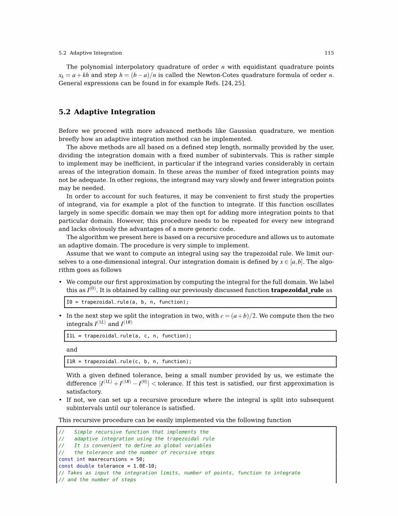
The algorithm we present here is based on a recursive procedure and allows us to automatean adaptive domain. The procedure is very simple to implement.
Assume that we want to compute an integral using say the trapezoidal rule. We limit our-selves to a one-dimensional integral. Our integration domain is defined by x $ [a,b]. The algo-rithm goes as follows
• We compute our first approximation by computing the integral for the full domain. We labelthis as I(0). It is obtained by calling our previously discussed function trapezoidal_rule as
I0 = trapezoidal_rule(a, b, n, function);
• In the next step we split the integration in two, with c= (a+b)/2. We compute then the twointegrals I(1L) and I(1R)
I1L = trapezoidal_rule(a, c, n, function);
and
I1R = trapezoidal_rule(c, b, n, function);
With a given defined tolerance, being a small number provided by us, we estimate thedifference |I(1L) + I(1R)! I(0)| < tolerance. If this test is satisfied, our first approximation issatisfactory.
• If not, we can set up a recursive procedure where the integral is split into subsequentsubintervals until our tolerance is satisfied.
This recursive procedure can be easily implemented via the following function
// Simple recursive function that implements the
// adaptive integration using the trapezoidal rule
// It is convenient to define as global variables
// the tolerance and the number of recursive steps
const int maxrecursions = 50;const double tolerance = 1.0E-10;// Takes as input the integration limits, number of points, function to integrate
// and the number of steps

116 5 Numerical Integration
void adaptive_integration(double a, double b, double *Integral, int n, int steps, double(*func)(double))
if ( steps > maxrecursions){cout << 'Too many recursive steps, the function varies too much' << endl;break;
}double c = (a+b)*0.5;// the whole integral
double I0 = trapezoidal_rule(a, b,n, func);// the left half
double I1L = trapezoidal_rule(a, c,n, func);// the right half
double I1R = trapezoidal_rule(c, b,n, func);
if (fabs(I1L+I1R-I0) < tolerance ) integral = I0;else
{adaptive_integration(a, c, integral, int n, ++steps, func)adaptive_integration(c, b, integral, int n, ++steps, func)
}
}// end function adaptive_integration
The variables integral and steps should be initialized to zero by the function that calls theadaptive procedure.
5.3 Gaussian Quadrature
The methods we have presented hitherto are taylored to problems where the mesh points xiare equidistantly spaced, xi differing from xi+1 by the step h. These methods are well suitedto cases where the integrand may vary strongly over a certain region or if we integrate overthe solution of a differential equation.
If however our integrand varies only slowly over a large interval, then the methods wehave discussed may only slowly converge towards a chosen precision1. As an example,
I =! b
1x!2 f (x)dx,
may converge very slowly to a given precision if b is large and/or f (x) varies slowly as functionof x at large values. One can obviously rewrite such an integral by changing variables to t= 1/xresulting in
I =! 1
b!1f (t!1)dt,
which has a small integration range and hopefully the number of mesh points needed is notthat large.
However, there are cases where no trick may help and where the time expenditure inevaluating an integral is of importance. For such cases we would like to recommend methodsbased on Gaussian quadrature. Here one can catch at least two birds with a stone, namely,increased precision and fewer integration points. But it is important that the integrand variessmoothly over the interval, else we have to revert to splitting the interval into many smallsubintervals and the gain achieved may be lost.
The basic idea behind all integration methods is to approximate the integral
1 You could e.g., impose that the integral should not change as function of increasing mesh points beyond thesixth digit.

5.3 Gaussian Quadrature 117
I =! b
af (x)dx"
N
∑i=1
ωi f (xi),
where ω and x are the weights and the chosen mesh points, respectively. In our previousdiscussion, these mesh points were fixed at the beginning, by choosing a given number ofpoints N. The weigths ω resulted then from the integration method we applied. Simpson’srule, see Eq. (5.6) would give
ω : {h/3,4h/3,2h/3,4h/3, . . .,4h/3,h/3},
for the weights, while the trapezoidal rule resulted in
ω : {h/2,h,h, . . . ,h,h/2} .
In general, an integration formula which is based on a Taylor series using N points, willintegrate exactly a polynomial P of degree N! 1. That is, the N weights ωn can be chosen tosatisfy N linear equations, see chapter 3 of Ref. [3]. A greater precision for a given amountof numerical work can be achieved if we are willing to give up the requirement of equallyspaced integration points. In Gaussian quadrature (hereafter GQ), both the mesh points andthe weights are to be determined. The points will not be equally spaced2. The theory behindGQ is to obtain an arbitrary weight ω through the use of so-called orthogonal polynomials.These polynomials are orthogonal in some interval say e.g., [-1,1]. Our points xi are chosen insome optimal sense subject only to the constraint that they should lie in this interval. Togetherwith the weights we have then 2N (N the number of points) parameters at our disposal.
Even though the integrand is not smooth, we could render it smooth by extracting from itthe weight function of an orthogonal polynomial, i.e., we are rewriting
I =! b
af (x)dx =
! b
aW (x)g(x)dx"
N
∑i=1
ωig(xi), (5.7)
where g is smooth and W is the weight function, which is to be associated with a givenorthogonal polynomial. Note that with a given weight function we end up evaluating theintegrand for the function g(xi).
The weight function W is non-negative in the integration interval x $ [a,b] such that forany n% 0, the integral
$ ba |x|nW (x)dx is integrable. The naming weight function arises from the
fact that it may be used to give more emphasis to one part of the interval than another. Aquadrature formula
! b
aW (x) f (x)dx "
N
∑i=1
ωi f (xi), (5.8)
with N distinct quadrature points (mesh points) is a called a Gaussian quadrature formula ifit integrates all polynomials p $ P2N!1 exactly, that is
! b
aW (x)p(x)dx =
N
∑i=1
ωi p(xi), (5.9)
It is assumed thatW (x) is continuous and positive and that the integral
! b
aW (x)dx
2 Typically, most points will be located near the origin, while few points are needed for large x values sincethe integrand is supposed to vary smoothly there. See below for an example.

118 5 Numerical Integration
exists. Note that the replacement of f &Wg is normally a better approximation due to thefact that we may isolate possible singularities ofW and its derivatives at the endpoints of theinterval.
The quadrature weights or just weights (not to be confused with the weight function) arepositive and the sequence of Gaussian quadrature formulae is convergent if the sequence QNof quadrature formulae
QN( f )&Q( f ) =! b
af (x)dx,
in the limit N& ∞. Then we say that the sequence
QN( f ) =N
∑i=1
ω(N)i f (x(N)i ),
is convergent for all polynomials p, that is
QN(p) = Q(p)
if there exits a constant C such thatN
∑i=1
|ω(N)i |'C,
for all N which are natural numbers.The error for the Gaussian quadrature formulae of order N is given by
! b
aW (x) f (x)dx!
N
∑k=1
wk f (xk) =f 2N(ξ )(2N)!
! b
aW (x)[qN(x)]2dx
where qN is the chosen orthogonal polynomial and ξ is a number in the interval [a,b]. Wehave assumed that f $ C2N [a,b], viz. the space of all real or complex 2N times continuouslydifferentiable functions.
In science there are several important orthogonal polynomials which arise from the solu-tion of differential equations. Well-known examples are the Legendre, Hermite, Laguerre andChebyshev polynomials. They have the following weight functions
Weight function Interval PolynomialW (x) = 1 x $ [!1,1] Legendre
W (x) = e!x2 !∞' x' ∞ HermiteW (x) = xαe!x 0' x' ∞ Laguerre
W (x) = 1/((1! x2) !1' x' 1 Chebyshev
The importance of the use of orthogonal polynomials in the evaluation of integrals can besummarized as follows.
• As stated above, methods based on Taylor series using N points will integrate exactly apolynomial P of degree N! 1. If a function f (x) can be approximated with a polynomial ofdegree N! 1
f (x) " PN!1(x),
with N mesh points we should be able to integrate exactly the polynomial PN!1.• Gaussian quadrature methods promise more than this. We can get a better polynomial
approximation with order greater than N to f (x) and still get away with only N mesh points.More precisely, we approximate
f (x)" P2N!1(x),
and with only N mesh points these methods promise that

5.3 Gaussian Quadrature 119
!f (x)dx "
!P2N!1(x)dx=
N!1
∑i=0
P2N!1(xi)ωi,
The reason why we can represent a function f (x) with a polynomial of degree 2N!1 is dueto the fact that we have 2N equations, N for the mesh points and N for the weights.
The mesh points are the zeros of the chosen orthogonal polynomial of order N, and theweights are determined from the inverse of a matrix. An orthogonal polynomials of degree Ndefined in an interval [a,b] has precisely N distinct zeros on the open interval (a,b).
Before we detail how to obtain mesh points and weights with orthogonal polynomials, letus revisit some features of orthogonal polynomials by specializing to Legendre polynomials.In the text below, we reserve hereafter the labelling LN for a Legendre polynomial of order N,while PN is an arbitrary polynomial of order N. These polynomials form then the basis for theGauss-Legendre method.
5.3.1 Orthogonal polynomials, Legendre
The Legendre polynomials are the solutions of an important differential equation in Science,namely
C(1! x2)P!m2l P+(1! x2) ddx
"(1! x2)dP
dx
#= 0.
Here C is a constant. For ml = 0 we obtain the Legendre polynomials as solutions, whereasml #= 0 yields the so-called associated Legendre polynomials. This differential equation arisesin for example the solution of the angular dependence of Schrödinger’s equation with spher-ically symmetric potentials such as the Coulomb potential.
The corresponding polynomials P are
Lk(x) =12kk!
dk
dxk(x2! 1)k k= 0,1,2, . . . ,
which, up to a factor, are the Legendre polynomials Lk. The latter fulfil the orthogonalityrelation ! 1
!1Li(x)Lj(x)dx=
22i+ 1
δi j , (5.10)
and the recursion relation
( j+ 1)Lj+1(x)+ jL j!1(x)! (2 j+ 1)xL j(x) = 0. (5.11)
It is common to choose the normalization condition
LN(1) = 1.
With these equations we can determine a Legendre polynomial of arbitrary order with inputpolynomials of order N! 1 and N! 2.
As an example, consider the determination of L0, L1 and L2. We have that
L0(x) = c,
with c a constant. Using the normalization equation L0(1) = 1 we get that
L0(x) = 1.

120 5 Numerical Integration
For L1(x) we have the general expression
L1(x) = a+ bx,
and using the orthogonality relation
! 1
!1L0(x)L1(x)dx= 0,
we obtain a= 0 and with the condition L1(1) = 1, we obtain b= 1, yielding
L1(x) = x.
We can proceed in a similar fashion in order to determine the coefficients of L2
L2(x) = a+ bx+ cx2,
using the orthogonality relations
! 1
!1L0(x)L2(x)dx= 0,
and ! 1
!1L1(x)L2(x)dx= 0,
and the condition L2(1) = 1 we would get
L2(x) =12%3x2! 1
&. (5.12)
We note that we have three equations to determine the three coefficients a, b and c.Alternatively, we could have employed the recursion relation of Eq. (5.11), resulting in
2L2(x) = 3xL1(x)!L0,
which leads to Eq. (5.12).The orthogonality relation above is important in our discussion on how to obtain the
weights and mesh points. Suppose we have an arbitrary polynomial QN!1 of order N!1 and aLegendre polynomial LN(x) of order N. We could represent QN!1 by the Legendre polynomialsthrough
QN!1(x) =N!1
∑k=0
αkLk(x), (5.13)
where αk’s are constants.Using the orthogonality relation of Eq. (5.10) we see that
! 1
!1LN(x)QN!1(x)dx=
N!1
∑k=0
! 1
!1LN(x)αkLk(x)dx= 0. (5.14)
We will use this result in our construction of mesh points and weights in the next subsection.In summary, the first few Legendre polynomials are
L0(x) = 1,
L1(x) = x,
L2(x) = (3x2! 1)/2,
5.3 Gaussian Quadrature 121
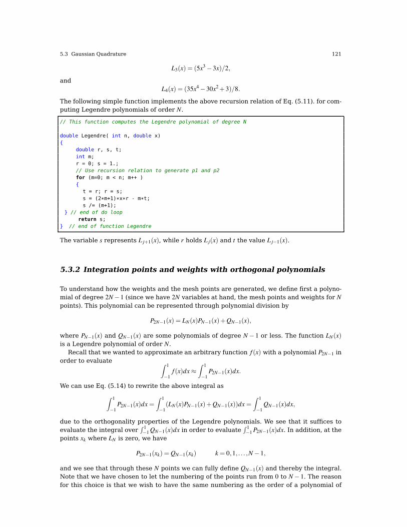
L3(x) = (5x3! 3x)/2,
andL4(x) = (35x4! 30x2+ 3)/8.
The following simple function implements the above recursion relation of Eq. (5.11). for com-puting Legendre polynomials of order N.
// This function computes the Legendre polynomial of degree N
double Legendre( int n, double x){
double r, s, t;
int m;r = 0; s = 1.;// Use recursion relation to generate p1 and p2
for (m=0; m < n; m++ ){
t = r; r = s;
s = (2*m+1)*x*r - m*t;s /= (m+1);
} // end of do loop
return s;} // end of function Legendre
The variable s represents Lj+1(x), while r holds Lj(x) and t the value Lj!1(x).
5.3.2 Integration points and weights with orthogonal polynomials
To understand how the weights and the mesh points are generated, we define first a polyno-mial of degree 2N!1 (since we have 2N variables at hand, the mesh points and weights for Npoints). This polynomial can be represented through polynomial division by
P2N!1(x) = LN(x)PN!1(x)+QN!1(x),
where PN!1(x) and QN!1(x) are some polynomials of degree N! 1 or less. The function LN(x)is a Legendre polynomial of order N.
Recall that we wanted to approximate an arbitrary function f (x) with a polynomial P2N!1 inorder to evaluate ! 1
!1f (x)dx"
! 1
!1P2N!1(x)dx.
We can use Eq. (5.14) to rewrite the above integral as
! 1
!1P2N!1(x)dx=
! 1
!1(LN(x)PN!1(x)+QN!1(x))dx=
! 1
!1QN!1(x)dx,
due to the orthogonality properties of the Legendre polynomials. We see that it suffices toevaluate the integral over
$ 1!1QN!1(x)dx in order to evaluate
$ 1!1P2N!1(x)dx. In addition, at the
points xk where LN is zero, we have
P2N!1(xk) = QN!1(xk) k= 0,1, . . . ,N! 1,
and we see that through these N points we can fully define QN!1(x) and thereby the integral.Note that we have chosen to let the numbering of the points run from 0 to N! 1. The reasonfor this choice is that we wish to have the same numbering as the order of a polynomial of

122 5 Numerical Integration
degree N! 1. This numbering will be useful below when we introduce the matrix elementswhich define the integration weights wi.
We develope then QN!1(x) in terms of Legendre polynomials, as done in Eq. (5.13),
QN!1(x) =N!1
∑i=0
αiLi(x). (5.15)
Using the orthogonality property of the Legendre polynomials we have
! 1
!1QN!1(x)dx=
N!1
∑i=0
αi! 1
!1L0(x)Li(x)dx= 2α0,
where we have just inserted L0(x) = 1! Instead of an integration problem we need now todefine the coefficient α0. Since we know the values of QN!1 at the zeros of LN , we may rewriteEq. (5.15) as
QN!1(xk) =N!1
∑i=0
αiLi(xk) =N!1
∑i=0
αiLik k= 0,1, . . . ,N! 1. (5.16)
Since the Legendre polynomials are linearly independent of each other, none of the columnsin the matrix Lik are linear combinations of the others. This means that the matrix Lik has aninverse with the properties
L!1L= I.
Multiplying both sides of Eq. (5.16) with ∑N!1j=0 L!1ji results in
N!1
∑i=0
(L!1)kiQN!1(xi) = αk. (5.17)
We can derive this result in an alternative way by defining the vectors
xk =
'
(((()
x0x1..
xN!1
*
++++,α =
'
(((()
α0α1..
αN!1
*
++++,,
and the matrix
L=
'
(()
L0(x0) L1(x0) . . . LN!1(x0)L0(x1) L1(x1) . . . LN!1(x1). . . . . . . . . . . .
L0(xN!1) L1(xN!1) . . . LN!1(xN!1)
*
++, .
We have thenQN!1(xk) = Lα,
yielding (if L has an inverse)L!1QN!1(xk) = α,
which is Eq. (5.17).Using the above results and the fact that
! 1
!1P2N!1(x)dx=
! 1
!1QN!1(x)dx,
we get
5.3 Gaussian Quadrature 123
! 1
!1P2N!1(x)dx=
! 1
!1QN!1(x)dx= 2α0 = 2
N!1
∑i=0
(L!1)0iP2N!1(xi).
If we identify the weights with 2(L!1)0i, where the points xi are the zeros of LN , we have anintegration formula of the type
! 1
!1P2N!1(x)dx=
N!1
∑i=0
ωiP2N!1(xi)
and if our function f (x) can be approximated by a polynomial P of degree 2N! 1, we havefinally that
! 1
!1f (x)dx "
! 1
!1P2N!1(x)dx=
N!1
∑i=0
ωiP2N!1(xi).
In summary, the mesh points xi are defined by the zeros of an orthogonal polynomial of degreeN, that is LN , while the weights are given by 2(L!1)0i.
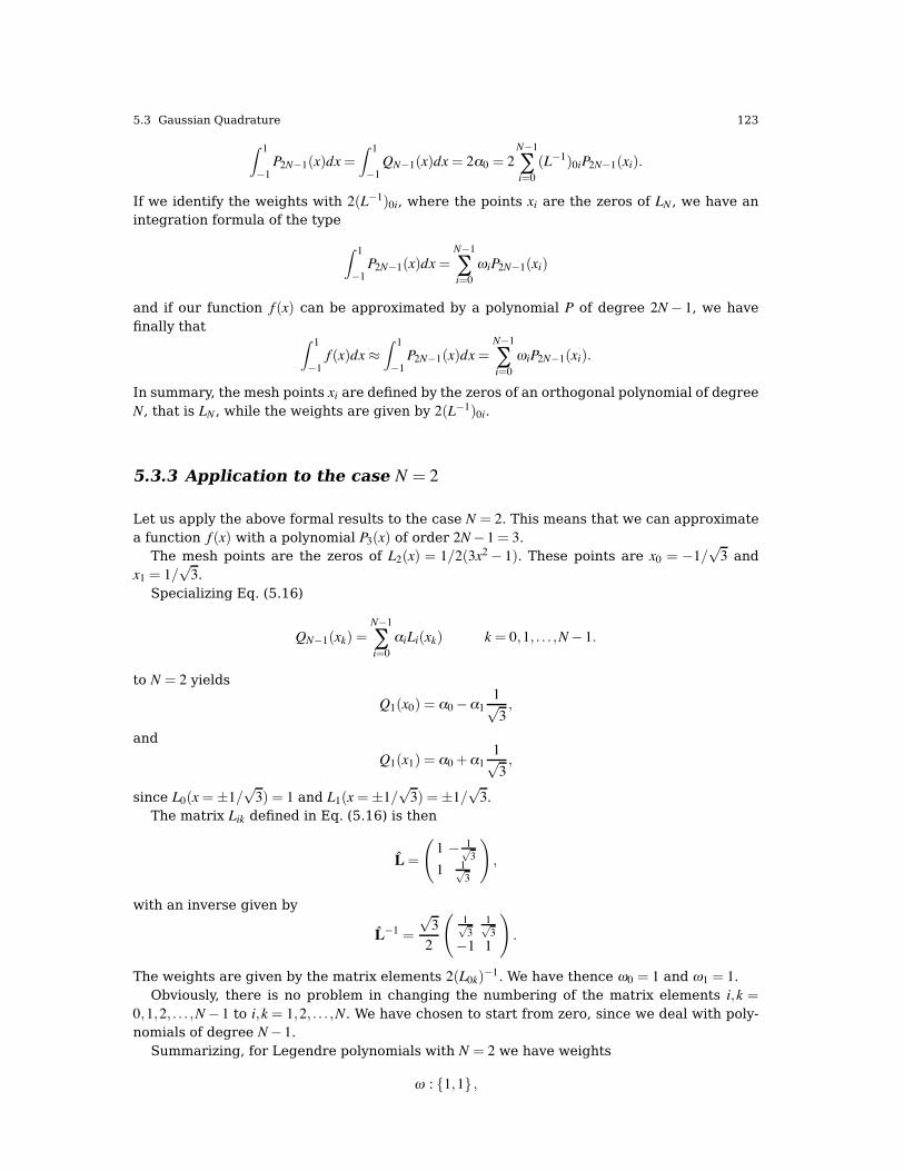
5.3.3 Application to the case N = 2
Let us apply the above formal results to the case N = 2. This means that we can approximatea function f (x) with a polynomial P3(x) of order 2N! 1= 3.
The mesh points are the zeros of L2(x) = 1/2(3x2! 1). These points are x0 = !1/(3 and
x1 = 1/(3.
Specializing Eq. (5.16)
QN!1(xk) =N!1
∑i=0
αiLi(xk) k = 0,1, . . . ,N! 1.
to N = 2 yieldsQ1(x0) = α0!α1
1(3,
and
Q1(x1) = α0+α11(3,
since L0(x=±1/(3) = 1 and L1(x=±1/
(3) =±1/
(3.
The matrix Lik defined in Eq. (5.16) is then
L=
-1 ! 1(
31 1(
3
.
,
with an inverse given by
L!1 =(32
-1(3
1(3
!1 1
.
.
The weights are given by the matrix elements 2(L0k)!1. We have thence ω0 = 1 and ω1 = 1.Obviously, there is no problem in changing the numbering of the matrix elements i,k =
0,1,2, . . . ,N! 1 to i,k = 1,2, . . . ,N. We have chosen to start from zero, since we deal with poly-nomials of degree N! 1.
Summarizing, for Legendre polynomials with N = 2 we have weights
ω : {1,1} ,

124 5 Numerical Integration
and mesh points
x :/!1(3,1(3
0.
If we wish to integrate ! 1
!1f (x)dx,
with f (x) = x2, we approximate
I =! 1
!1x2dx"
N!1
∑i=0
ωix2i .
The exact answer is 2/3. Using N = 2 with the above two weights and mesh points we get
I =! 1
!1x2dx=
1
∑i=0
ωix2i =13+13=23,
the exact answer!If we were to emply the trapezoidal rule we would get
I =! 1
!1x2dx=
b! a2%(a)2+(b)2
&/2= 1! (!1)
2%(!1)2+(1)2
&/2= 1!
With just two points we can calculate exactly the integral for a second-order polynomial sinceour methods approximates the exact function with higher order polynomial. How many pointsdo you need with the trapezoidal rule in order to achieve a similar accuracy?
5.3.4 General integration intervals for Gauss-Legendre
Note that the Gauss-Legendre method is not limited to an interval [-1,1], since we can alwaysthrough a change of variable
t =b! a2
x+b+ a2
,
rewrite the integral for an interval [a,b]
! b
af (t)dt =
b! a2
! 1
!1f"(b! a)x2
+b+ a2
#dx.
If we have an integral on the form ! ∞
0f (t)dt,
we can choose new mesh points and weights by using the mapping
xi = tan1π4(1+ xi)
2,
andωi =
π4
ωicos2
%π4 (1+ xi)
& ,
where xi and ωi are the original mesh points and weights in the interval [!1,1], while xi andωi are the new mesh points and weights for the interval [0,∞).
To see that this is correct by inserting the the value of xi =!1 (the lower end of the interval[!1,1]) into the expression for xi. That gives xi = 0, the lower end of the interval [0,∞). Forxi = 1, we obtain xi = ∞. To check that the new weights are correct, recall that the weights

5.3 Gaussian Quadrature 125
should correspond to the derivative of the mesh points. Try to convince yourself that theabove expression fulfills this condition.
5.3.5 Other orthogonal polynomials
5.3.5.1 Laguerre polynomials
If we are able to rewrite our integral of Eq. (5.7) with a weight function W (x) = xαe!x withintegration limits [0,∞), we could then use the Laguerre polynomials. The polynomials formthen the basis for the Gauss-Laguerre method which can be applied to integrals of the form
I =! ∞
0f (x)dx =
! ∞
0xαe!xg(x)dx.
These polynomials arise from the solution of the differential equation
"d2
dx2!
ddx
+λx!l(l+ 1)x2
#L (x) = 0,
where l is an integer l% 0 and λ a constant. This equation arises for example from the solutionof the radial Schrödinger equation with a centrally symmetric potential such as the Coulombpotential. The first few polynomials are
L0(x) = 1,
L1(x) = 1! x,
L2(x) = 2! 4x+ x2,
L3(x) = 6! 18x+ 9x2! x3,
andL4(x) = x4! 16x3+ 72x2! 96x+ 24.
They fulfil the orthogonality relation! ∞
0e!xLn(x)2dx= 1,
and the recursion relation
(n+ 1)Ln+1(x) = (2n+ 1! x)Ln(x)! nLn!1(x).
5.3.5.2 Hermite polynomials
In a similar way, for an integral which goes like
I =! ∞
!∞f (x)dx =
! ∞
!∞e!x
2g(x)dx.
we could use the Hermite polynomials in order to extract weights and mesh points. TheHermite polynomials are the solutions of the following differential equation
d2H(x)dx2
! 2xdH(x)dx
+(λ ! 1)H(x) = 0.

126 5 Numerical Integration
A typical example is again the solution of Schrödinger’s equation, but this time with a har-monic oscillator potential. The first few polynomials are
H0(x) = 1,
H1(x) = 2x,
H2(x) = 4x2! 2,
H3(x) = 8x3! 12,
andH4(x) = 16x4! 48x2+ 12.
They fulfil the orthogonality relation! ∞
!∞e!x
2Hn(x)2dx= 2nn!
(π,
and the recursion relationHn+1(x) = 2xHn(x)! 2nHn!1(x).
5.3.6 Applications to selected integrals
Before we proceed with some selected applications, it is important to keep in mind that sincethe mesh points are not evenly distributed, a careful analysis of the behavior of the integrandas function of x and the location of mesh points is mandatory. To give you an example, inthe Table below we show the mesh points and weights for the integration interval [0,100]for N = 10 points obtained by the Gauss-Legendre method. Clearly, if your function oscillates
Table 5.1 Mesh points and weights for the integration interval [0,100] with N = 10 using the Gauss-Legendremethod.
i xi ωi1 1.305 3.3342 6.747 7.4733 16.030 10.9544 28.330 13.4635 42.556 14.7766 57.444 14.7767 71.670 13.4638 83.970 10.9549 93.253 7.473
10 98.695 3.334
strongly in any subinterval, this approach needs to be refined, either by choosing more pointsor by choosing other integration methods. Note also that for integration intervals like forexample x $ [0,∞], the Gauss-Legendre method places more points at the beginning of theintegration interval. If your integrand varies slowly for large values of x, then this methodmay be appropriate.
Let us here compare three methods for integrating, namely the trapezoidal rule, Simpson’smethod and the Gauss-Legendre approach. We choose two functions to integrate:
5.3 Gaussian Quadrature 127
! 100
1
exp(!x)x
dx,
and ! 3
0
12+ x2
dx.
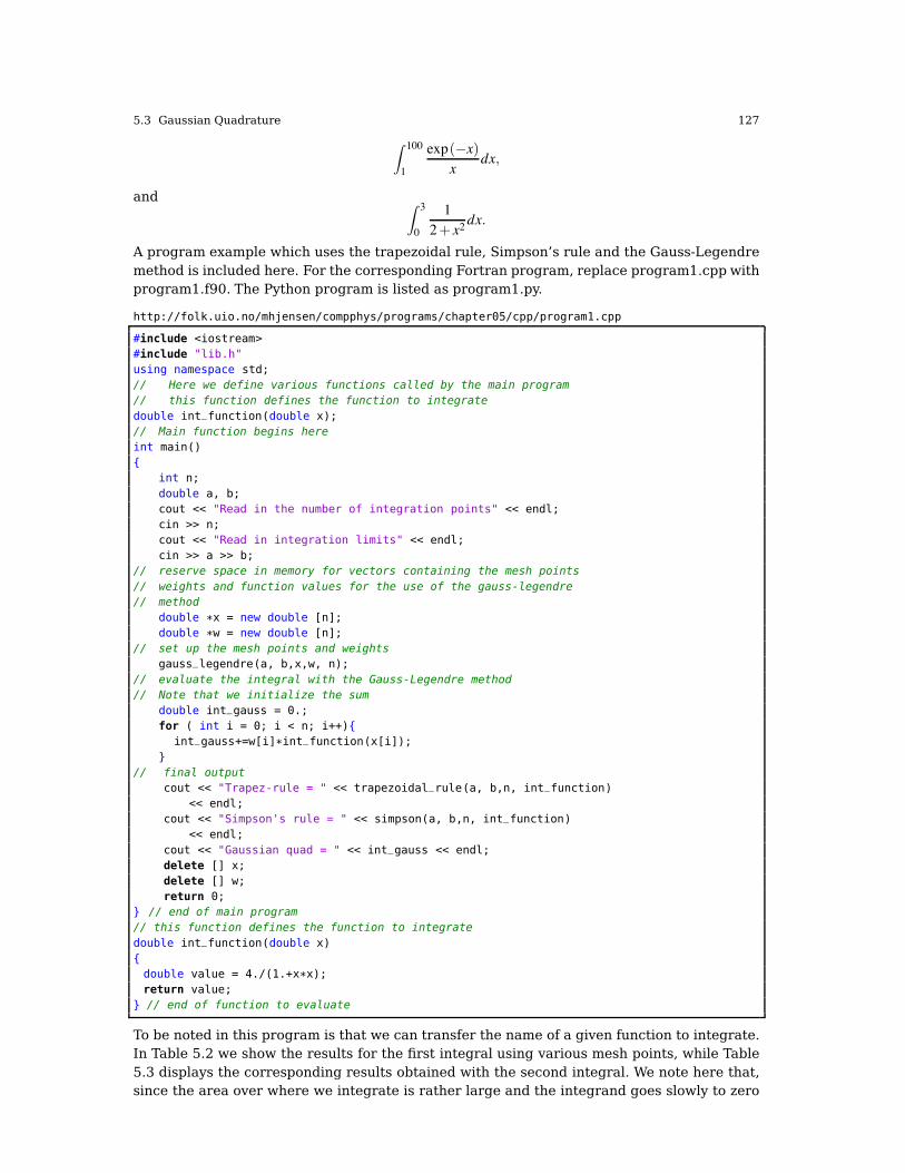
A program example which uses the trapezoidal rule, Simpson’s rule and the Gauss-Legendremethod is included here. For the corresponding Fortran program, replace program1.cpp withprogram1.f90. The Python program is listed as program1.py.
http://folk.uio.no/mhjensen/compphys/programs/chapter05/cpp/program1.cpp
#include <iostream>#include "lib.h"using namespace std;// Here we define various functions called by the main program
// this function defines the function to integrate
double int_function(double x);// Main function begins here
int main(){
int n;
double a, b;cout << "Read in the number of integration points" << endl;cin >> n;cout << "Read in integration limits" << endl;cin >> a >> b;
// reserve space in memory for vectors containing the mesh points
// weights and function values for the use of the gauss-legendre
// method
double *x = new double [n];double *w = new double [n];
// set up the mesh points and weights
gauss_legendre(a, b,x,w, n);
// evaluate the integral with the Gauss-Legendre method
// Note that we initialize the sum
double int_gauss = 0.;for ( int i = 0; i < n; i++){
int_gauss+=w[i]*int_function(x[i]);}
// final output
cout << "Trapez-rule = " << trapezoidal_rule(a, b,n, int_function)<< endl;
cout << "Simpson's rule = " << simpson(a, b,n, int_function)<< endl;
cout << "Gaussian quad = " << int_gauss << endl;delete [] x;delete [] w;return 0;
} // end of main program
// this function defines the function to integrate
double int_function(double x){double value = 4./(1.+x*x);return value;
} // end of function to evaluate
To be noted in this program is that we can transfer the name of a given function to integrate.In Table 5.2 we show the results for the first integral using various mesh points, while Table5.3 displays the corresponding results obtained with the second integral. We note here that,since the area over where we integrate is rather large and the integrand goes slowly to zero
128 5 Numerical Integration
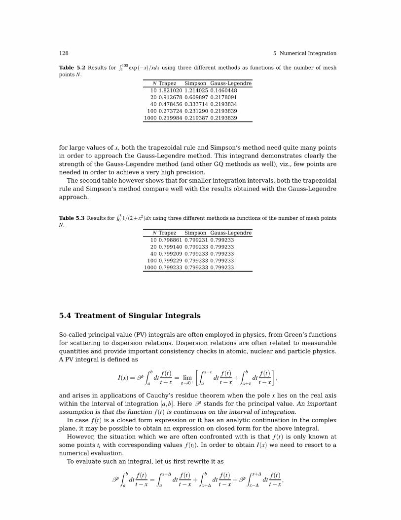
Table 5.2 Results for$ 1001 exp (!x)/xdx using three different methods as functions of the number of mesh
points N.N Trapez Simpson Gauss-Legendre10 1.821020 1.214025 0.146044820 0.912678 0.609897 0.217809140 0.478456 0.333714 0.2193834
100 0.273724 0.231290 0.21938391000 0.219984 0.219387 0.2193839
for large values of x, both the trapezoidal rule and Simpson’s method need quite many pointsin order to approach the Gauss-Legendre method. This integrand demonstrates clearly thestrength of the Gauss-Legendre method (and other GQ methods as well), viz., few points areneeded in order to achieve a very high precision.
The second table however shows that for smaller integration intervals, both the trapezoidalrule and Simpson’s method compare well with the results obtained with the Gauss-Legendreapproach.
Table 5.3 Results for$ 30 1/(2+x2)dx using three different methods as functions of the number of mesh points
N.N Trapez Simpson Gauss-Legendre10 0.798861 0.799231 0.79923320 0.799140 0.799233 0.79923340 0.799209 0.799233 0.799233
100 0.799229 0.799233 0.7992331000 0.799233 0.799233 0.799233
5.4 Treatment of Singular Integrals
So-called principal value (PV) integrals are often employed in physics, from Green’s functionsfor scattering to dispersion relations. Dispersion relations are often related to measurablequantities and provide important consistency checks in atomic, nuclear and particle physics.A PV integral is defined as
I(x) = P
! b
adtf (t)t! x
= limε&0+
3! x!ε
adtf (t)t! x
+! b
x+εdtf (t)t! x
4,
and arises in applications of Cauchy’s residue theorem when the pole x lies on the real axiswithin the interval of integration [a,b]. Here P stands for the principal value. An importantassumption is that the function f (t) is continuous on the interval of integration.
In case f (t) is a closed form expression or it has an analytic continuation in the complexplane, it may be possible to obtain an expression on closed form for the above integral.
However, the situation which we are often confronted with is that f (t) is only known atsome points ti with corresponding values f (ti). In order to obtain I(x) we need to resort to anumerical evaluation.
To evaluate such an integral, let us first rewrite it as
P
! b
adtf (t)t! x
=! x!Δ
adtf (t)t! x
+! b
x+Δdtf (t)t! x
+P
! x+Δ
x!Δdtf (t)t! x
,
5.4 Treatment of Singular Integrals 129
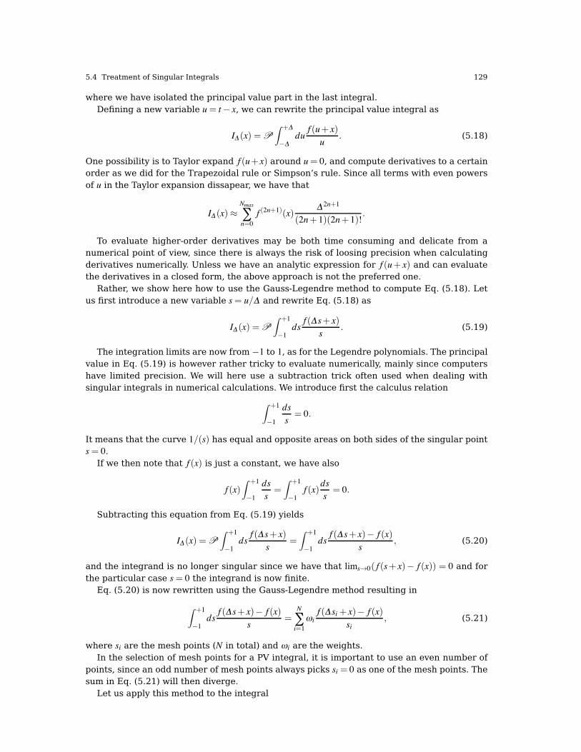
where we have isolated the principal value part in the last integral.Defining a new variable u= t! x, we can rewrite the principal value integral as
IΔ (x) = P
! +Δ
!Δdu
f (u+ x)u
. (5.18)
One possibility is to Taylor expand f (u+x) around u= 0, and compute derivatives to a certainorder as we did for the Trapezoidal rule or Simpson’s rule. Since all terms with even powersof u in the Taylor expansion dissapear, we have that
IΔ (x)"Nmax∑n=0
f (2n+1)(x)Δ2n+1
(2n+ 1)(2n+ 1)!.
To evaluate higher-order derivatives may be both time consuming and delicate from anumerical point of view, since there is always the risk of loosing precision when calculatingderivatives numerically. Unless we have an analytic expression for f (u+ x) and can evaluatethe derivatives in a closed form, the above approach is not the preferred one.
Rather, we show here how to use the Gauss-Legendre method to compute Eq. (5.18). Letus first introduce a new variable s= u/Δ and rewrite Eq. (5.18) as
IΔ (x) = P
! +1
!1dsf (Δs+ x)
s. (5.19)
The integration limits are now from !1 to 1, as for the Legendre polynomials. The principalvalue in Eq. (5.19) is however rather tricky to evaluate numerically, mainly since computershave limited precision. We will here use a subtraction trick often used when dealing withsingular integrals in numerical calculations. We introduce first the calculus relation
! +1
!1
dss= 0.
It means that the curve 1/(s) has equal and opposite areas on both sides of the singular points= 0.
If we then note that f (x) is just a constant, we have also
f (x)! +1
!1
dss
=! +1
!1f (x)
dss
= 0.
Subtracting this equation from Eq. (5.19) yields
IΔ (x) = P
! +1
!1dsf (Δs+ x)
s=! +1
!1dsf (Δs+ x)! f (x)
s, (5.20)
and the integrand is no longer singular since we have that lims&0( f (s+ x)! f (x)) = 0 and forthe particular case s= 0 the integrand is now finite.
Eq. (5.20) is now rewritten using the Gauss-Legendre method resulting in
! +1
!1dsf (Δs+ x)! f (x)
s=
N
∑i=1
ωif (Δsi+ x)! f (x)
si, (5.21)
where si are the mesh points (N in total) and ωi are the weights.In the selection of mesh points for a PV integral, it is important to use an even number of
points, since an odd number of mesh points always picks si = 0 as one of the mesh points. Thesum in Eq. (5.21) will then diverge.
Let us apply this method to the integral

130 5 Numerical Integration
I(x) = P
! +1
!1dtet
t. (5.22)
The integrand diverges at x= t = 0. We rewrite it using Eq. (5.20) as
P
! +1
!1dtet
t=! +1
!1
et ! 1t
, (5.23)
since ex = e0 = 1. With Eq. (5.21) we have then
! +1
!1
et ! 1t"
N
∑i=1
ωieti ! 1ti
. (5.24)
The exact results is 2.11450175075.....With just two mesh points we recall from the previoussubsection that ω1=ω2= 1 and that the mesh points are the zeros of L2(x), namely x1=!1/
(3
and x2 = 1/(3. Setting N = 2 and inserting these values in the last equation gives
I2(x= 0) =(35e1/(3! e!1/
(36= 2.1129772845.
With six mesh points we get even the exact result to the tenth digit
I6(x= 0) = 2.11450175075!
We can repeat the above subtraction trick for more complicated integrands. First we mod-ify the integration limits to ±∞ and use the fact that
! ∞
!∞
dkk! k0
=! 0
!∞
dkk! k0
+! ∞
0
dkk! k0
= 0.
A change of variable u=!k in the integral with limits from !∞ to 0 gives! ∞
!∞
dkk! k0
=! 0
∞
!du!u! k0
+! ∞
0
dkk! k0
=! ∞
0
dk!k! k0
+! ∞
0
dkk! k0
= 0.
It means that the curve 1/(k! k0) has equal and opposite areas on both sides of the singularpoint k0. If we break the integral into one over positive k and one over negative k, a change ofvariable k&!k allows us to rewrite the last equation as
! ∞
0
dkk2! k20
= 0.
We can use this to express a principal values integral as
P
! ∞
0
f (k)dkk2! k20
=! ∞
0
( f (k)! f (k0))dkk2! k20
, (5.25)
where the right-hand side is no longer singular at k = k0, it is proportional to the derivatived f/dk, and can be evaluated numerically as any other integral.
Such a trick is often used when evaluating integral equations, as discussed in the nextsection.

5.5 Parallel Computing 131
5.5 Parallel Computing
We end this chapter by discussing modern supercomputing concepts like parallel computing.In particular, we will introduce you to the usage of the Message Passing Interface (MPI) li-brary. MPI is a library, not a programming language. It specifies the names, calling sequencesand results of functions or subroutines to be called from C++ or Fortran programs, and theclasses and methods that make up the MPI C++ library. The programs that users write inFortran or C++ are compiled with ordinary compilers and linked with the MPI library. MPIprograms should be able to run on all possible machines and run all MPI implementetationswithout change. An excellent reference is the text by Karniadakis and Kirby II [17].
5.5.1 Brief survey of supercomputing concepts and terminologies
Since many discoveries in science are nowadays obtained via large-scale simulations, thereis an ever-lasting wish and need to do larger simulations using shorter computer time. Thedevelopment of the capacity for single-processor computers (even with increased processorspeed and memory) can hardly keep up with the pace of scientific computing. The solution tothe needs of the scientific computing and high-performance computing (HPC) communitieshas therefore been parallel computing.
The basic ideas of parallel computing is that multiple processors are involved to solve aglobal problem. The essence is to divide the entire computation evenly among collaborativeprocessors.
Today’s supercomputers are parallel machines and can achieve peak performances almostup to 1015 floating point operations per second, so-called peta-scale computers, see for ex-ample the list over the world’s top 500 supercomputers at www.top500.org. This list getsupdated twice per year and sets up the ranking according to a given supercomputer’s perfor-mance on a benchmark code from the LINPACK library. The benchmark solves a set of linearequations using the best software for a given platform.
To understand the basic philosophy, it is useful to have a rough picture of how to clas-sify different hardware models. We distinguish betwen three major groups, (i) conventionalsingle-processor computers, normally called SISD (single-instruction-single-data) machines,(ii) so-called SIMD machines (single-instruction-multiple-data), which incorporate the idea ofparallel processing using a large number of processing units to execute the same instruc-tion on different data and finally (iii) modern parallel computers, so-called MIMD (multiple-instruction- multiple-data) machines that can execute different instruction streams in parallelon different data. On a MIMD machine the different parallel processing units perform op-erations independently of each others, only subject to synchronization via a given messagepassing interface at specified time intervals. MIMDmachines are the dominating ones amongpresent supercomputers, and we distinguish between two types of MIMD computers, namelyshared memory machines and distributed memory machines. In shared memory systems thecentral processing units (CPU) share the same address space. Any CPU can access any data inthe global memory. In distributed memory systems each CPU has its own memory. The CPUsare connected by some network and may exchange messages. A recent trend are so-calledccNUMA (cache-coherent-non-uniform-memory- access) systems which are clusters of SMP(symmetric multi-processing) machines and have a virtual shared memory.
Distributed memory machines, in particular those based on PC clusters, are nowadays themost widely used and cost-effective, although farms of PC clusters require large infrastuc-tures and yield additional expenses for cooling. PC clusters with Linux as operating systemsare easy to setup and offer several advantages, since they are built from standard commodity

132 5 Numerical Integration
hardware with the open source software (Linux) infrastructure. The designer can improveperformance proportionally with added machines. The commodity hardware can be any ofa number of mass-market, stand-alone compute nodes as simple as two networked comput-ers each running Linux and sharing a file system or as complex as thousands of nodes witha high-speed, low-latency network. In addition to the increased speed of present individualprocessors (and most machines come today with dual cores or four cores, so-called quad-cores) the position of such commodity supercomputers has been strenghtened by the factthat a library like MPI has made parallel computing portable and easy. Although there areseveral implementations, they share the same core commands. Message-passing is a matureprogramming paradigm and widely accepted. It often provides an efficient match to the hard-ware.
5.5.2 Parallelism
When we discuss parallelism, it is common to subdivide different algorithms in three majorgroups.
• Task parallelism:the work of a global problem can be divided into a number of inde-pendent tasks, which rarely need to synchronize. Monte Carlo simulations and numericalintegration are examples of possible applications. Since there is more or less no commu-nication between different processors, task parallelism results in almost a perfect mathe-matical parallelism and is commonly dubbed embarassingly parallel (EP). The examples inthis chapter fall under that category. The use of the MPI library is then limited to some fewfunction calls and the programming is normally very simple.
• Data parallelism: use of multiple threads (e.g., one thread per processor) to dissect loopsover arrays etc. This paradigm requires a single memory address space. Communicationand synchronization between the processors are often hidden, and it is thus easy to pro-gram. However, the user surrenders much control to a specialized compiler. An example ofdata parallelism is compiler-based parallelization.
• Message-passing: all involved processors have an independent memory address space.The user is responsible for partitioning the data/work of a global problem and distribut-ing the subproblems to the processors. Collaboration between processors is achieved byexplicit message passing, which is used for data transfer plus synchronization.This paradigm is the most general one where the user has full control. Better parallelefficiency is usually achieved by explicit message passing. However, message-passing pro-gramming is more difficult. We will meet examples of this in connection with the solutioneigenvalue problems in chapter 7 and of partial differential equations in chapter 10.
Before we proceed, let us look at two simple examples. We will also use these simpleexamples to define the speedup factor of a parallel computation. The first case is that of theadditions of two vectors of dimension n,
z= αx+βy,
where α and β are two real or complex numbers and z,x,y $ Rn or $ Cn. For every elementwe have thus
zi = αxi+βyi.
For every element zi we have three floating point operations, two multiplications and oneaddition. If we assume that these operations take the same time Δ t, then the total time spentby one processor is
5.5 Parallel Computing 133
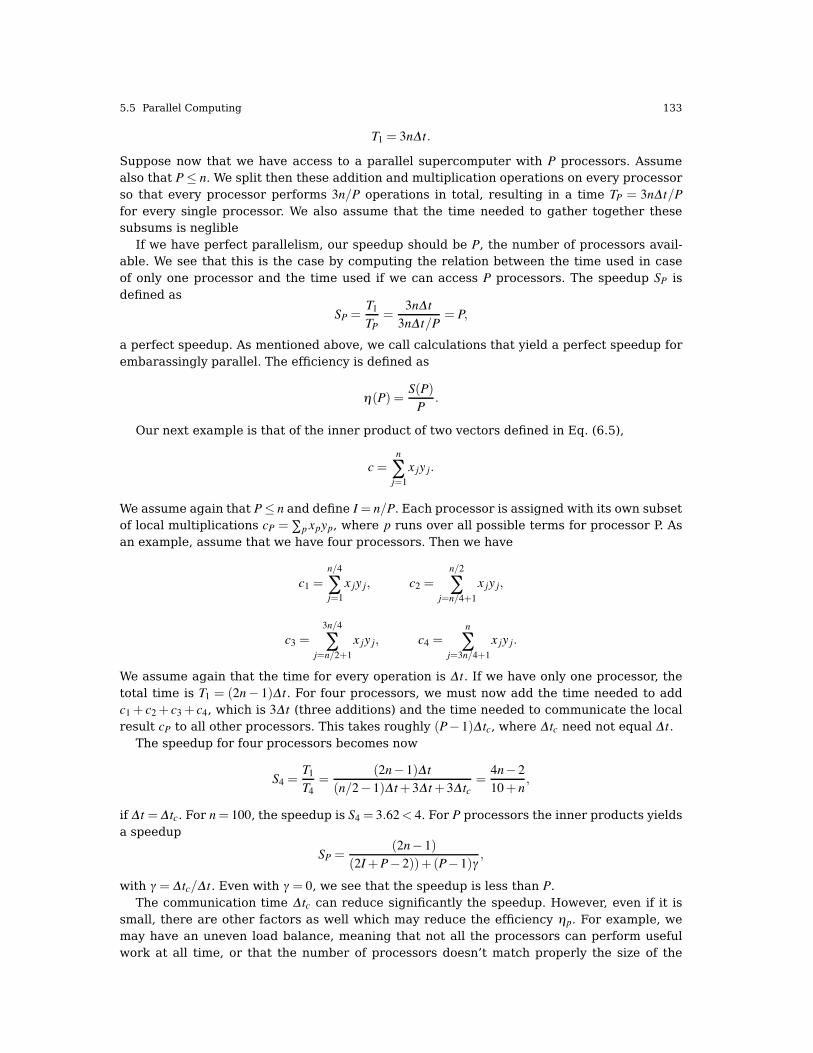
T1 = 3nΔ t.
Suppose now that we have access to a parallel supercomputer with P processors. Assumealso that P' n. We split then these addition and multiplication operations on every processorso that every processor performs 3n/P operations in total, resulting in a time TP = 3nΔ t/Pfor every single processor. We also assume that the time needed to gather together thesesubsums is neglible
If we have perfect parallelism, our speedup should be P, the number of processors avail-able. We see that this is the case by computing the relation between the time used in caseof only one processor and the time used if we can access P processors. The speedup SP isdefined as
SP =T1TP
=3nΔ t3nΔ t/P
= P,
a perfect speedup. As mentioned above, we call calculations that yield a perfect speedup forembarassingly parallel. The efficiency is defined as
η(P) =S(P)P
.
Our next example is that of the inner product of two vectors defined in Eq. (6.5),
c=n
∑j=1
x jy j.
We assume again that P' n and define I= n/P. Each processor is assigned with its own subsetof local multiplications cP = ∑p xpyp, where p runs over all possible terms for processor P. Asan example, assume that we have four processors. Then we have
c1 =n/4
∑j=1
x jy j, c2 =n/2
∑j=n/4+1
x jy j,
c3 =3n/4
∑j=n/2+1
x jy j, c4 =n
∑j=3n/4+1
x jy j.
We assume again that the time for every operation is Δ t. If we have only one processor, thetotal time is T1 = (2n! 1)Δ t. For four processors, we must now add the time needed to addc1+ c2+ c3+ c4, which is 3Δ t (three additions) and the time needed to communicate the localresult cP to all other processors. This takes roughly (P! 1)Δ tc, where Δ tc need not equal Δ t.
The speedup for four processors becomes now
S4 =T1T4
=(2n! 1)Δ t
(n/2! 1)Δ t+ 3Δ t+ 3Δ tc=4n! 210+ n
,
if Δ t = Δ tc. For n= 100, the speedup is S4 = 3.62< 4. For P processors the inner products yieldsa speedup
SP =(2n! 1)
(2I+P! 2))+ (P! 1)γ,
with γ = Δ tc/Δ t. Even with γ = 0, we see that the speedup is less than P.The communication time Δ tc can reduce significantly the speedup. However, even if it is
small, there are other factors as well which may reduce the efficiency ηp. For example, wemay have an uneven load balance, meaning that not all the processors can perform usefulwork at all time, or that the number of processors doesn’t match properly the size of the

134 5 Numerical Integration
problem, or memory problems, or that a so-called startup time penalty known as latency mayslow down the transfer of data. Crucial here is the rate at which messages are transferred
5.5.3 MPI with simple examples
When we want to parallelize a sequential algorithm, there are at least two aspects we needto consider, namely
• Identify the part(s) of a sequential algorithm that can be executed in parallel. This can bedifficult.
• Distribute the global work and data among P processors. Stated differently, here you needto understand how you can get computers to run in parallel. From a practical point of viewit means to implement parallel programming tools.
In this chapter we focus mainly on the last point. MPI is then a tool for writing programsto run in parallel, without needing to know much (in most cases nothing) about a given ma-chine’s architecture. MPI programs work on both shared memory and distributed memorymachines. Furthermore, MPI is a very rich and complicated library. But it is not necessary touse all the features. The basic and most used functions have been optimized for most machinearchitectures
Before we proceed, we need to clarify some concepts, in particular the usage of the wordsprocess and processor. We refer to process as a logical unit which executes its own code,in an MIMD style. The processor is a physical device on which one or several processes areexecuted. The MPI standard uses the concept process consistently throughout its documen-tation. However, since we only consider situations where one processor is responsible for oneprocess, we therefore use the two terms interchangeably in the discussion below, hopefullywithout creating ambiguities.
The six most important MPI functions are
• MPI_ Init - initiate an MPI computation• MPI_Finalize - terminate the MPI computation and clean up• MPI_Comm_size - how many processes participate in a given MPI computation.• MPI_Comm_rank - which rank does a given process have. The rank is a number between 0
and size-1, the latter representing the total number of processes.• MPI_Send - send a message to a particular process within an MPI computation• MPI_Recv - receive a message from a particular process within an MPI computation.
The first MPI C++ program is a rewriting of our ’hello world’ program (without the com-putation of the sine function) from chapter 2. We let every process write "Hello world" on thestandard output.
http://folk.uio.no/mhjensen/compphys/programs/chapter05/program2.cpp
// First C++ example of MPI Hello world
using namespace std;#include <mpi.h>#include <iostream>
int main (int nargs, char* args[])
{int numprocs, my_rank;
// MPI initializations
MPI_Init (&nargs, &args);MPI_Comm_size (MPI_COMM_WORLD, &numprocs);MPI_Comm_rank (MPI_COMM_WORLD, &my_rank);

5.5 Parallel Computing 135
cout << "Hello world, I have rank " << my_rank << " out of " << numprocs << endl;// End MPI
MPI_Finalize ();return 0;
}
The corresponding Fortran program reads
PROGRAM helloINCLUDE "mpif.h"INTEGER:: numprocs, my_rank, ierr
CALL MPI_INIT(ierr)CALL MPI_COMM_SIZE(MPI_COMM_WORLD, numprocs, ierr)CALL MPI_COMM_RANK(MPI_COMM_WORLD, my_rank, ierr)WRITE(*,*)"Hello world, I've rank ",my_rank," out of ",numprocsCALL MPI_FINALIZE(ierr)
END PROGRAM hello
MPI is a message-passing library where all the routines have a corresponding C++-bindings3
MPI_Command_name or Fortran-bindings (function names are by convention in uppercase, but canalso be in lower case) MPI_COMMAND_NAME
To use the MPI library you must include header files which contain definitions and decla-rations that are needed by the MPI library routines. The following line must appear at the topof any source code file that will make an MPI call. For Fortran you must put in the beginningof your program the declaration
INCLUDE 'mpif.h'
while for C++ you need to include the statement
#include "mpi.h"
These header files contain the declarations of functions, variabels etc. needed by the MPIlibrary.
The first MPI call must be MPI_INIT, which initializes the message passing routines, asdefined in for example
INTEGER :: ierrCALL MPI_INIT(ierr)
for the Fortran example. The variable ierr is an integer which holds an error code whenthe call returns. The value of ierr is however of little use since, by default, MPI aborts theprogram when it encounters an error. However, ierr must be included when MPI starts. Forthe C++ code we have the call to the function
MPI_Init(int *argc, char *argv)
where argc and argv are arguments passed to main. MPI does not use these arguments in anyway, however, and in MPI-2 implementations, NULL may be passed instead. When you havefinished you must call the function MPI_Finalize. In Fortran you use the statement
CALL MPI_FINALIZE(ierr)
3 The C++ bindings used in practice are the same as the C bindings, although reading older texts like [15–17]one finds extensive discussions on the difference between C and C++ bindings. Throughout this text we willuse the C bindings.

136 5 Numerical Integration
while for C++ we use the function MPI_Finalize().In addition to these calls, we have also included calls to so-called inquiry functions. There
are two MPI calls that are usually made soon after initialization. They are for C++,
MPI_COMM_SIZE((MPI_COMM_WORLD, &numprocs)
and
CALL MPI_COMM_SIZE(MPI_COMM_WORLD, numprocs, ierr)
for Fortran. The function MPI_COMM_SIZE returns the number of tasks in a specified MPI com-municator (comm when we refer to it in generic function calls below).
In MPI you can divide your total number of tasks into groups, called communicators. Whatdoes that mean? All MPI communication is associated with what one calls a communicatorthat describes a group of MPI processes with a name (context). The communicator desig-nates a collection of processes which can communicate with each other. Every process isthen identified by its rank. The rank is only meaningful within a particular communicator. Acommunicator is thus used as a mechanism to identify subsets of processes. MPI has the flex-ibility to allow you to define different types of communicators, see for example [16]. However,here we have used the communicator MPI_COMM_WORLD that contains all the MPI processes thatare initiated when we run the program.
The variable numprocs refers to the number of processes we have at our disposal. The func-tion MPI_COMM_RANK returns the rank (the name or identifier) of the tasks running the code. Eachtask (or processor) in a communicator is assigned a number my_rank from 0 to numprocs! 1.
We are now ready to perform our first MPI calculations.
5.5.3.1 Running codes with MPI
To compile and load the above C++ code (after having understood how to use a local cluster),we can use the command
mpicxx -O2 -o program2.x program2.cpp
and try to run with ten nodes using the command
mpiexec -np 10 ./program2.x
If we wish to use the Fortran version we need to replace the C++ compiler statement mpiccwith mpif90 or equivalent compilers. The name of the compiler is obviously system dependent.The command mpirunmay be used instead of mpiexec. Here you need to check your own system.
When we run MPI all processes use the same binary executable version of the code andall processes are running exactly the same code. The question is then how can we tell thedifference between our parallel code running on a given number of processes and a serialcode? There are two major distinctions you should keep in mind: (i) MPI lets each processhave a particular rank to determine which instructions are run on a particular process and (ii)the processes communicate with each other in order to finalize a task. Even if all processesreceive the same set of instructions, they will normally not execute the same instructions.Wewill discuss this point in connection with our integration example below.
The above example produces the following output

5.5 Parallel Computing 137
Hello world, I’ve rank 0 out of 10 procs.
Hello world, I’ve rank 1 out of 10 procs.
Hello world, I’ve rank 4 out of 10 procs.
Hello world, I’ve rank 3 out of 10 procs.
Hello world, I’ve rank 9 out of 10 procs.
Hello world, I’ve rank 8 out of 10 procs.
Hello world, I’ve rank 2 out of 10 procs.
Hello world, I’ve rank 5 out of 10 procs.
Hello world, I’ve rank 7 out of 10 procs.
Hello world, I’ve rank 6 out of 10 procs.
The output to screen is not ordered since all processes are trying to write to screen simul-taneously. It is then the operating system which opts for an ordering. If we wish to have anorganized output, starting from the first process, we may rewrite our program as follows
http://folk.uio.no/mhjensen/compphys/programs/chapter05/program3.cpp
// Second C++ example of MPI Hello world
using namespace std;#include <mpi.h>#include <iostream>
int main (int nargs, char* args[]){
int numprocs, my_rank, i;// MPI initializations
MPI_Init (&nargs, &args);MPI_Comm_size (MPI_COMM_WORLD, &numprocs);MPI_Comm_rank (MPI_COMM_WORLD, &my_rank);for (i = 0; i < numprocs; i++) {
MPI_Barrier (MPI_COMM_WORLD);if (i == my_rank) {cout << "Hello world, I have rank " << my_rank << " out of " << numprocs << endl;fflush (stdout);
}}
// End MPI
MPI_Finalize ();return 0;
}
Here we have used the MPI_Barrier function to ensure that every process has completed its setof instructions in a particular order. A barrier is a special collective operation that does notallow the processes to continue until all processes in the communicator (here MPI_COMM_WORLD)have called MPI_Barrier. The output is now
Hello world, I’ve rank 0 out of 10 procs.
Hello world, I’ve rank 1 out of 10 procs.
Hello world, I’ve rank 2 out of 10 procs.
Hello world, I’ve rank 3 out of 10 procs.
Hello world, I’ve rank 4 out of 10 procs.
Hello world, I’ve rank 5 out of 10 procs.
Hello world, I’ve rank 6 out of 10 procs.
138 5 Numerical Integration
Hello world, I’ve rank 7 out of 10 procs.
Hello world, I’ve rank 8 out of 10 procs.
Hello world, I’ve rank 9 out of 10 procs.
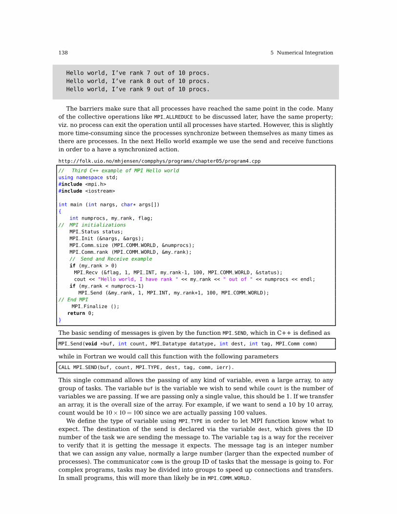
The barriers make sure that all processes have reached the same point in the code. Manyof the collective operations like MPI_ALLREDUCE to be discussed later, have the same property;viz. no process can exit the operation until all processes have started. However, this is slightlymore time-consuming since the processes synchronize between themselves as many times asthere are processes. In the next Hello world example we use the send and receive functionsin order to a have a synchronized action.
http://folk.uio.no/mhjensen/compphys/programs/chapter05/program4.cpp
// Third C++ example of MPI Hello world
using namespace std;#include <mpi.h>#include <iostream>
int main (int nargs, char* args[]){
int numprocs, my_rank, flag;// MPI initializations
MPI_Status status;MPI_Init (&nargs, &args);MPI_Comm_size (MPI_COMM_WORLD, &numprocs);MPI_Comm_rank (MPI_COMM_WORLD, &my_rank);
// Send and Receive example
if (my_rank > 0)MPI_Recv (&flag, 1, MPI_INT, my_rank-1, 100, MPI_COMM_WORLD, &status);cout << "Hello world, I have rank " << my_rank << " out of " << numprocs << endl;
if (my_rank < numprocs-1)MPI_Send (&my_rank, 1, MPI_INT, my_rank+1, 100, MPI_COMM_WORLD);
// End MPI
MPI_Finalize ();return 0;
}
The basic sending of messages is given by the function MPI_SEND, which in C++ is defined as
MPI_Send(void *buf, int count, MPI_Datatype datatype, int dest, int tag, MPI_Comm comm)
while in Fortran we would call this function with the following parameters
CALL MPI_SEND(buf, count, MPI_TYPE, dest, tag, comm, ierr).
This single command allows the passing of any kind of variable, even a large array, to anygroup of tasks. The variable buf is the variable we wish to send while count is the number ofvariables we are passing. If we are passing only a single value, this should be 1. If we transferan array, it is the overall size of the array. For example, if we want to send a 10 by 10 array,count would be 10) 10= 100 since we are actually passing 100 values.
We define the type of variable using MPI_TYPE in order to let MPI function know what toexpect. The destination of the send is declared via the variable dest, which gives the IDnumber of the task we are sending the message to. The variable tag is a way for the receiverto verify that it is getting the message it expects. The message tag is an integer numberthat we can assign any value, normally a large number (larger than the expected number ofprocesses). The communicator comm is the group ID of tasks that the message is going to. Forcomplex programs, tasks may be divided into groups to speed up connections and transfers.In small programs, this will more than likely be in MPI_COMM_WORLD.

5.5 Parallel Computing 139
Furthermore, when an MPI routine is called, the Fortran or C++ data type which is passedmust match the corresponding MPI integer constant. An integer is defined as MPI_INT in C++and MPI_INTEGER in Fortran. A double precision real is MPI_DOUBLE in C++ and MPI_DOUBLE_PRECISION
in Fortran and single precision real is MPI_FLOAT in C++ and MPI_REAL in Fortran. For furtherdefinitions of data types see chapter five of Ref. [16].
Once you have sent a message, you must receive it on another task. The function MPI_RECV
is similar to the send call. In C++ we would define this as
MPI_Recv( void *buf, int count, MPI_Datatype datatype, int source, int tag, MPI_Comm comm,MPI_Status *status )
while in Fortran we would use the call
CALL MPI_RECV(buf, count, MPI_TYPE, source, tag, comm, status, ierr)}.
The arguments that are different from those in MPI_SEND are buf which is the name of thevariable where you will be storing the received data, source which replaces the destination inthe send command. This is the return ID of the sender.
Finally, we have used MPI_Status~status;where one can check if the receive was completed.The source or tag of a received message may not be known if wildcard values are used in thereceive function. In C++, MPI Status is a structure that contains further information. Onecan obtain this information using
MPI_Get_count (MPI_Status *status, MPI_Datatype datatype, int *count)}
The output of this code is the same as the previous example, but now process 0 sends amessage to process 1, which forwards it further to process 2, and so forth.
Armed with this wisdom, performed all hello world greetings, we are now ready for seriouswork.
5.5.4 Numerical integration with MPI
To integrate numerically with MPI we need to define how to send and receive data types. Thismeans also that we need to specify which data types to send to MPI functions.
The program listed here integrates
π =! 1
0dx
41+ x2
by simply adding up areas of rectangles according to the algorithm discussed in Eq. (5.5),rewritten here
I =! b
af (x)dx " h
N
∑i=1
f (xi!1/2),
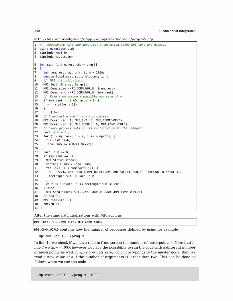
where f (x) = 4/(1+ x2). This is a brute force way of obtaining an integral but suffices todemonstrate our first application of MPI to mathematical problems. What we do is to subdi-vide the integration range x $ [0,1] into n rectangles. Increasing n should obviously increasethe precision of the result, as discussed in the beginning of this chapter. The parallel partproceeds by letting every process collect a part of the sum of the rectangles. At the end ofthe computation all the sums from the processes are summed up to give the final global sum.The program below serves thus as a simple example on how to integrate in parallel. We willrefine it in the next examples and we will also add a simple example on how to implement thetrapezoidal rule.
140 5 Numerical Integration
http://folk.uio.no/mhjensen/compphys/programs/chapter05/program5.cpp
1 // Reactangle rule and numerical integration using MPI send and Receive
2 using namespace std;3 #include <mpi.h>4 #include <iostream>
5 int main (int nargs, char* args[])6 {7 int numprocs, my_rank, i, n = 1000;8 double local_sum, rectangle_sum, x, h;9 // MPI initializations
10 MPI_Init (&nargs, &args);
11 MPI_Comm_size (MPI_COMM_WORLD, &numprocs);12 MPI_Comm_rank (MPI_COMM_WORLD, &my_rank);13 // Read from screen a possible new vaue of n
14 if (my_rank == 0 && nargs > 1) {15 n = atoi(args[1]);
16 }17 h = 1.0/n;18 // Broadcast n and h to all processes
19 MPI_Bcast (&n, 1, MPI_INT, 0, MPI_COMM_WORLD);20 MPI_Bcast (&h, 1, MPI_DOUBLE, 0, MPI_COMM_WORLD);21 // Every process sets up its contribution to the integral
22 local_sum = 0.;23 for (i = my_rank; i < n; i += numprocs) {24 x = (i+0.5)*h;25 local_sum += 4.0/(1.0+x*x);26 }27 local_sum *= h;
28 if (my_rank == 0) {29 MPI_Status status;30 rectangle_sum = local_sum;31 for (i=1; i < numprocs; i++) {32 MPI_Recv(&local_sum,1,MPI_DOUBLE,MPI_ANY_SOURCE,500,MPI_COMM_WORLD,&status);33 rectangle_sum += local_sum;
34 }35 cout << "Result: " << rectangle_sum << endl;36 } else
37 MPI_Send(&local_sum,1,MPI_DOUBLE,0,500,MPI_COMM_WORLD);38 // End MPI
39 MPI_Finalize ();
40 return 0;41 }
After the standard initializations with MPI such as
MPI_Init, MPI_Comm_size, MPI_Comm_rank,
MPI_COMM_WORLD contains now the number of processes defined by using for example
mpirun -np 10 ./prog.x
In line 14 we check if we have read in from screen the number of mesh points n. Note that inline 7 we fix n= 1000, however we have the possibility to run the code with a different numberof mesh points as well. If my_rank equals zero, which correponds to the master node, then weread a new value of n if the number of arguments is larger than two. This can be done asfollows when we run the code
mpiexec -np 10 ./prog.x 10000

5.5 Parallel Computing 141
In line 17 we define also the step length h. In lines 19 and 20 we use the broadcast functionMPI_Bcast. We use this particular function because we want data on one processor (our masternode) to be shared with all other processors. The broadcast function sends data to a group ofprocesses. The MPI routine MPI_Bcast transfers data from one task to a group of others. Theformat for the call is in C++ given by the parameters of
MPI_Bcast (&n, 1, MPI_INT, 0, MPI_COMM_WORLD);.
In case we have a floating point variable we need to declare
MPI_Bcast (&h, 1, MPI_DOUBLE, 0, MPI_COMM_WORLD);
The general structure of this function is
MPI_Bcast( void *buf, int count, MPI_Datatype datatype, int root, MPI_Comm comm)
All processes call this function, both the process sending the data (with rank zero) and allthe other processes in MPI_COMM_WORLD. Every process has now copies of n and h, the numberof mesh points and the step length, respectively.
We transfer the addresses of n and h. The second argument represents the number ofdata sent. In case of a one-dimensional array, one needs to transfer the number of arrayelements. If you have an n)mmatrix, you must transfer n)m. We need also to specify whetherthe variable type we transfer is a non-numerical such as a logical or character variable ornumerical of the integer, real or complex type.
We transfer also an integer variable int root. This variable specifies the process whichhas the original copy of the data. Since we fix this value to zero in the call in lines 19 and 20,it means that it is the master process which keeps this information. For Fortran, this functionis called via the statement
CALL MPI_BCAST(buff, count, MPI_TYPE, root, comm, ierr).
In lines 23-27, every process sums its own part of the final sum used by the rectangle rule.The receive statement collects the sums from all other processes in case my_rank==0, else anMPI send is performed.
The above function is not very elegant. Furthermore, the MPI instructions can be simplifiedby using the functions MPI_Reduce or MPI_Allreduce. The first function takes information from allprocesses and sends the result of the MPI operation to one process only, typically the masternode. If we use MPI_Allreduce, the result is sent back to all processes, a feature which is usefulwhen all nodes need the value of a joint operation. We limit ourselves to MPI_Reduce since it isonly one process which will print out the final number of our calculation, The arguments toMPI_Allreduce are the same.
The MPI_Reduce function is defined as follows
MPI_Reduce( void *senddata, void* resultdata, int count, MPI_Datatype datatype, MPI_Op, introot, MPI_Comm comm)
The two variables senddata and resultdata are obvious, besides the fact that one sends theaddress of the variable or the first element of an array. If they are arrays they need to have thesame size. The variable count represents the total dimensionality, 1 in case of just one variable,while MPI_Datatype defines the type of variable which is sent and received. The new feature isMPI_Op. MPI_Op defines the type of operation we want to do. There are many options, see againRefs. [15–17] for full list. In our case, since we are summing the rectangle contributions fromevery process we define MPI_Op=MPI_SUM. If we have an array or matrix we can search for thelargest og smallest element by sending either MPI_MAX or MPI_MIN. If we want the location aswell (which array element) we simply transfer MPI_MAXLOC or MPI_MINOC. If we want the productwe write MPI_PROD. MPI_Allreduce is defined as
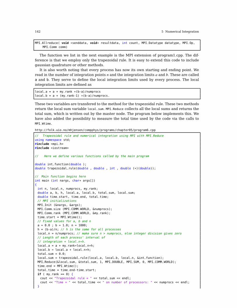
142 5 Numerical Integration
MPI_Allreduce( void *senddata, void* resultdata, int count, MPI_Datatype datatype, MPI_Op,MPI_Comm comm)
The function we list in the next example is the MPI extension of program1.cpp. The dif-ference is that we employ only the trapezoidal rule. It is easy to extend this code to includegaussian quadrature or other methods.
It is also worth noting that every process has now its own starting and ending point. Weread in the number of integration points n and the integration limits a and b. These are calleda and b. They serve to define the local integration limits used by every process. The localintegration limits are defined as
local_a = a + my_rank *(b-a)/numprocslocal_b = a + (my_rank-1) *(b-a)/numprocs.
These two variables are transfered to the method for the trapezoidal rule. These two methodsreturn the local sum variable local_sum. MPI_Reduce collects all the local sums and returns thetotal sum, which is written out by the master node. The program below implements this. Wehave also added the possibility to measure the total time used by the code via the calls toMPI_Wtime.
http://folk.uio.no/mhjensen/compphys/programs/chapter05/program6.cpp
// Trapezoidal rule and numerical integration using MPI with MPI_Reduce
using namespace std;#include <mpi.h>#include <iostream>
// Here we define various functions called by the main program
double int_function(double );double trapezoidal_rule(double , double , int , double (*)(double));
// Main function begins here
int main (int nargs, char* args[]){int n, local_n, numprocs, my_rank;double a, b, h, local_a, local_b, total_sum, local_sum;double time_start, time_end, total_time;// MPI initializations
MPI_Init (&nargs, &args);MPI_Comm_size (MPI_COMM_WORLD, &numprocs);MPI_Comm_rank (MPI_COMM_WORLD, &my_rank);time_start = MPI_Wtime();// Fixed values for a, b and n
a = 0.0 ; b = 1.0; n = 1000;
h = (b-a)/n; // h is the same for all processes
local_n = n/numprocs; // make sure n > numprocs, else integer division gives zero
// Length of each process' interval of
// integration = local_n*h.
local_a = a + my_rank*local_n*h;
local_b = local_a + local_n*h;total_sum = 0.0;local_sum = trapezoidal_rule(local_a, local_b, local_n, &int_function);MPI_Reduce(&local_sum, &total_sum, 1, MPI_DOUBLE, MPI_SUM, 0, MPI_COMM_WORLD);time_end = MPI_Wtime();total_time = time_end-time_start;
if ( my_rank == 0) {cout << "Trapezoidal rule = " << total_sum << endl;cout << "Time = " << total_time << " on number of processors: " << numprocs << endl;
}
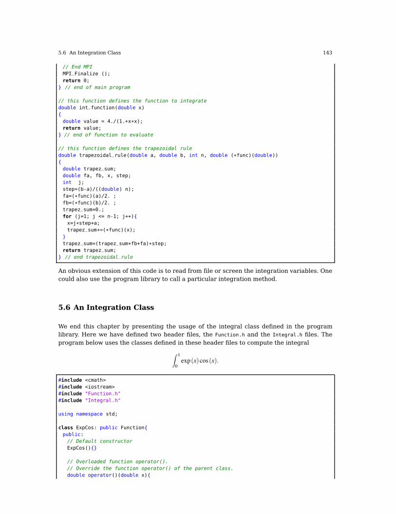
5.6 An Integration Class 143
// End MPI
MPI_Finalize ();
return 0;} // end of main program
// this function defines the function to integrate
double int_function(double x){
double value = 4./(1.+x*x);return value;
} // end of function to evaluate
// this function defines the trapezoidal rule
double trapezoidal_rule(double a, double b, int n, double (*func)(double)){double trapez_sum;double fa, fb, x, step;int j;step=(b-a)/((double) n);
fa=(*func)(a)/2. ;fb=(*func)(b)/2. ;trapez_sum=0.;for (j=1; j <= n-1; j++){x=j*step+a;trapez_sum+=(*func)(x);
}trapez_sum=(trapez_sum+fb+fa)*step;return trapez_sum;
} // end trapezoidal_rule
An obvious extension of this code is to read from file or screen the integration variables. Onecould also use the program library to call a particular integration method.
5.6 An Integration Class
We end this chapter by presenting the usage of the integral class defined in the programlibrary. Here we have defined two header files, the Function.h and the Integral.h files. Theprogram below uses the classes defined in these header files to compute the integral
! 1
0exp(x)cos(x).
#include <cmath>#include <iostream>#include "Function.h"#include "Integral.h"
using namespace std;
class ExpCos: public Function{public:// Default constructor
ExpCos(){}
// Overloaded function operator().
// Override the function operator() of the parent class.
double operator()(double x){

144 5 Numerical Integration
return exp(x)*cos(x);}
};
int main(){// Declare first an object of the function to be integrated
ExpCos f;// Set integration bounds
double a = 0.0; // Lower bound
double b = 1.0; // Upper bound
int npts = 100; // Number of integration points
// Declared (lhs) and instantiate an integral object of type Trapezoidal
Integral *trapez = new Trapezoidal(a, b, npts, f);Integral *midpt = new MidPoint(a, b, npts, f);Integral *gl = new Gauss_Legendre(a,b,npts, f);
// Evaluate the integral of the function ExpCos and assign its
// value to the variable result;
double resultTP = trapez->evaluate();double resultMP = midpt->evaluate();double resultGL = gl->evaluate();
// Print the result to screen
cout << "Result with trapezoidal : " << resultTP << endl;cout << "Result with mid-point : " << resultMP << endl;cout << "Result with Gauss-Legendre: " << resultGL << endl;
}
The header file Function.h is defined as
http://folk.uio.no/mhjensen/compphys/programs/chapter05/cpp/Function.h
/**
* @file Function.h
* Interface for mathematical functions with one or more independent variables.
* The subclasses are implemented as functors, i.e., objects behaving as functions.
* They overload the function operator().
*
* Example Usage:
// 1. Declare a functor, i.e., an object which
// overloads the function operator().
class Squared: public Function{public:
// Overload function operator()
double operator()(double x=0.0){return x*x;
}};
int main(){// Instance an object Functor
Squared f;
// Use the instance of the object as a normal function
cout << f(3.0) << endl;
}@endcode
*
**/

5.6 An Integration Class 145
#ifndef FUNCTION_H#define FUNCTION_H
#include "Array.h"
class Function{public:
//! Destructor
virtual ~Function(){}; // Not needed here.
/**
* @brief Overload the function operator().
*
* Used for evaluating functions with one independent variable.
*
**/
virtual double operator()(double x){}
/**
* @brief Overload the function operator().
*
* Used for evaluating functions with more than one independent variable.
**/
virtual double operator()(const Array<double>& x){}
};#endif
The header file Integral.h contains, with an example on how to use it, the following state-ments
http://folk.uio.no/mhjensen/compphys/programs/chapter05/cpp/Integral.h
#ifndef INTEGRAL_H#define INTEGRAL_H
#include "Array.h"#include "Function.h"#include <cmath>
class Integral{protected: // Access in the subclasses.
double a; // Lower limit of integration.
double b; // Upper limit of integration.
int npts; // Number of integration points.
Function &f; // Function to be integrated.
public:
/**
* @brief Constructor.
*
* @param lower_. Lower limit of integration.
* @param upper_. Upper limit of integration.
* @param npts_. Number of points of integration.
* @param f_. Reference to a functor representing the function to be integrated.
**/
Integral(double lower_, double upper_, int npts_, Function &f_);
//! Destructor
virtual ~Integral(){}

146 5 Numerical Integration
/**
* @brief Evaluate the integral.
* @return The value of the integral in double precision.
**/
virtual double evaluate()=0;
// virtual forloop
}; // End class Integral
class Trapezoidal: public Integral{
private:double h; // Step size.
public:/**
* @brief Constructor.
*
* @param lower_. Lower limit of integration.
* @param upper_. Upper limit of integration.
* @param npts_. Number of points of integration.
* @param f_. Reference to a functor representing the function to be integrated.
**/
Trapezoidal(double lower_, double upper_, int npts_, Function &f_);
//! Destructor
~Trapezoidal(){}
/**
* Evaluate the integral of a function f using the trapezoidal rule.
* @return The value of the integral in double precision.
**/
double evaluate();}; // End class Trapezoidal
class MidPoint: public Integral{private:double h; // Step size.
public:
/**
* @brief Constructor.
*
* @param lower_. Lower limit of integration.
* @param upper_. Upper limit of integration.
* @param npts_. Number of points of integration.
* @param f_. Reference to a functor representing the function to be integrated.
**/
MidPoint(double lower_, double upper_, int npts_, Function &f_);
//! Destructor
~MidPoint(){}
/**
* Evaluate the integral of a function f using the midpoint approximation.
*
* @return The value of the integral in double precision.
**/
double evaluate();
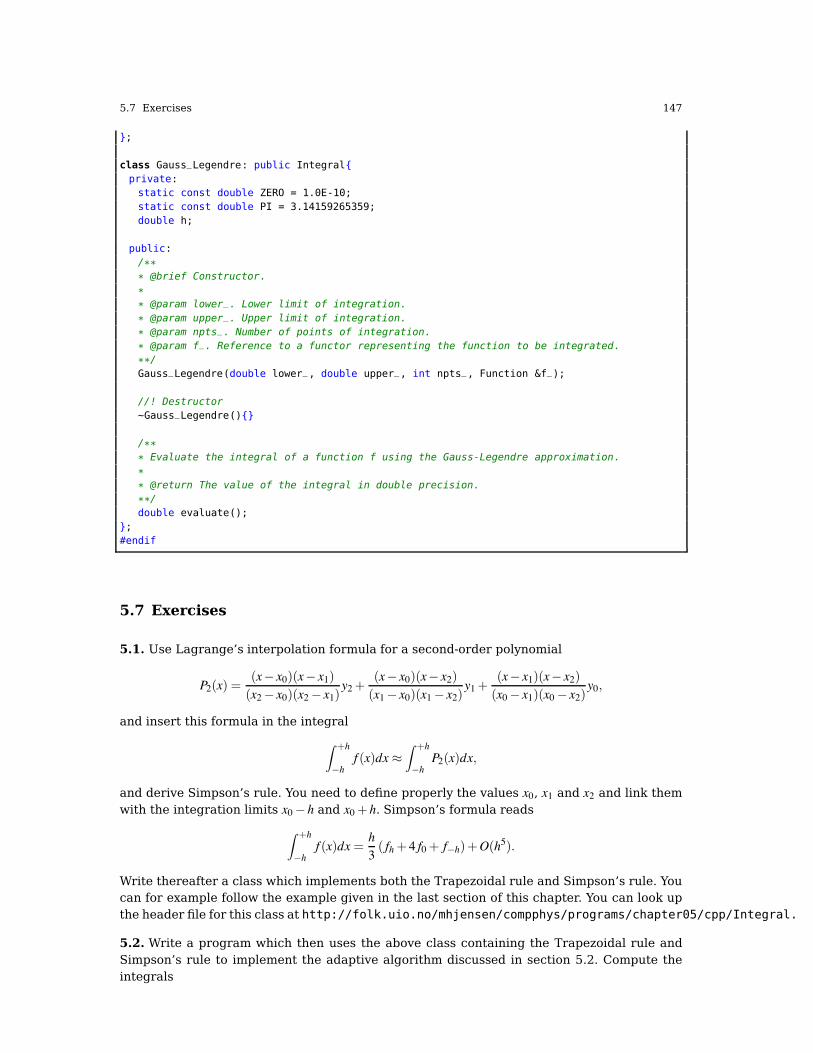
5.7 Exercises 147
};
class Gauss_Legendre: public Integral{private:static const double ZERO = 1.0E-10;static const double PI = 3.14159265359;double h;
public:/**
* @brief Constructor.
*
* @param lower_. Lower limit of integration.
* @param upper_. Upper limit of integration.
* @param npts_. Number of points of integration.
* @param f_. Reference to a functor representing the function to be integrated.
**/
Gauss_Legendre(double lower_, double upper_, int npts_, Function &f_);
//! Destructor
~Gauss_Legendre(){}
/**
* Evaluate the integral of a function f using the Gauss-Legendre approximation.
*
* @return The value of the integral in double precision.
**/
double evaluate();};#endif
5.7 Exercises
5.1. Use Lagrange’s interpolation formula for a second-order polynomial
P2(x) =(x! x0)(x! x1)(x2! x0)(x2! x1)
y2+(x! x0)(x! x2)(x1! x0)(x1! x2)
y1+(x! x1)(x! x2)(x0! x1)(x0! x2)
y0,
and insert this formula in the integral
! +h
!hf (x)dx "
! +h
!hP2(x)dx,
and derive Simpson’s rule. You need to define properly the values x0, x1 and x2 and link themwith the integration limits x0! h and x0+ h. Simpson’s formula reads
! +h
!hf (x)dx=
h3( fh+ 4 f0+ f!h)+O(h5).
Write thereafter a class which implements both the Trapezoidal rule and Simpson’s rule. Youcan for example follow the example given in the last section of this chapter. You can look upthe header file for this class at http://folk.uio.no/mhjensen/compphys/programs/chapter05/cpp/Integral.h.
5.2. Write a program which then uses the above class containing the Trapezoidal rule andSimpson’s rule to implement the adaptive algorithm discussed in section 5.2. Compute theintegrals
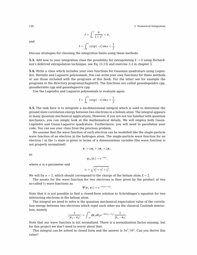
148 5 Numerical Integration
I =! 1
0
41+ x2
= π ,
and
I =! ∞
0xexp(!x)sinx= 1
2.
Discuss strategies for choosing the integration limits using these methods
5.3. Add now to your integration class the possibility for extrapolating h& 0 using Richard-son’s deferred extrapolation technique, see Eq. (3.13) and exercise 3.2 in chapter 3.
5.4. Write a class which includes your own functions for Gaussian quadrature using Legen-dre, Hermite and Laguerre polynomials. You can write your own functions for these methodsor use those included with the programs of this book. For the latter see for example theprograms in the directory programs/chapter05. The functions are called gausslegendre.cpp,gausshermite.cpp and gausslaguerre.cpp.
Use the Legendre and Laguerre polynomials to evaluate again
I =! ∞
0xexp(!x)sinx= 1
2.
5.5. The task here is to integrate a six-dimensional integral which is used to determine theground state correlation energy between two electrons in a helium atom. The integral appearsin many quantum mechanical applications. However, if you are not too familiar with quantummechanics, you can simply look at the mathematical details. We will employ both Gauss-Legendre and Gauss-Laguerre quadrature. Furthermore, you will need to parallelize yourcode. You can use your class from the previous problem.
We assume that the wave function of each electron can be modelled like the single-particlewave function of an electron in the hydrogen atom. The single-particle wave function for anelectron i in the 1s state is given in terms of a dimensionless variable (the wave function isnot properly normalized)
ri = xiex+ yiey+ ziez,
asψ1s(ri) = e!αri ,
where α is a parameter and
ri =7x2i + y2i + z2i .
We will fix α = 2, which should correspond to the charge of the helium atom Z = 2.The ansatz for the wave function for two electrons is then given by the product of two
so-called 1s wave functions asΨ(r1,r2) = e!α(r1+r2).
Note that it is not possible to find a closed-form solution to Schrödinger’s equation for twointeracting electrons in the helium atom.
The integral we need to solve is the quantum mechanical expectation value of the correla-tion energy between two electrons which repel each other via the classical Coulomb interac-tion, namely
*1
|r1! r2|+=
! ∞
!∞dr1dr2e!2α(r1+r2)
1|r1! r2|
.
Note that our wave function is not normalized. There is a normalization factor missing, butfor this project we don’t need to worry about that.
This integral can be solved in closed form and the answer is 5π2/162. Can you derive thisvalue?

5.7 Exercises 149
1. Use Gauss-Legendre quadrature and compute the integral by integrating for each variablex1,y1,z1,x2,y2,z2 from !∞ to ∞. How many mesh points do you need before the results con-verges at the level of the third leading digit? Hint: the single-particle wave function e!αri ismore or less zero at ri "? (find the appropriate limit). You can therefore replace the integra-tion limits !∞ and ∞ with !? and ?, respectively. You need to check that this approximationis satisfactory, that is, make a plot of the function and check if the abovementioned limitsare appropriate. You need also to account for the potential problems which may arise when|r1! r2|= 0.
2. The Legendre polynomials are defined for x $ [!1,1]. The previous exercise gave a veryunsatisfactory ad hoc procedure. We wish to improve our results. It can therefore be usefulto change to another coordinate frame and employ the Laguerre polynomials. The Laguerrepolynomials are defined for x $ [0,∞) and if we change to spherical coordinates
dr1dr2 = r21dr1r22dr2dcos(θ1)dcos(θ2)dφ1dφ2,
with1r12
=17
r21+ r22! 2r1r2cos(β )
andcos(β ) = cos(θ1)cos(θ2)+ sin(θ1)sin(θ2)cos(φ1!φ2))
we can rewrite the above integral with different integration limits. Find these limits andreplace the Gauss-Legendre approach in a) with Laguerre polynomials. Do your resultsimprove? Compare with the results from a).
3. Make a detailed analysis of the time used by both methods and compare your results.Parallelize your codes and check that you have an optimal speed up.