numerical data analysis - universiti sains …medic.usm.my/biostat/files/documents/basic...
TRANSCRIPT

1
NUMERICAL DATA ANALYSIS
Univariable Univariate Analysis of Numerical Data (Parametric)
Introduction
• Numerical data the outcome is numerical
• Univariable analysis concern with only 1 independent variable
• Univariate analysis concern with only 1 dependent variable
• Parametric normal distribution of the outcome variable

2
Introduction
• Three most commonly used statistical test in this group;
– Independent t-test
– Paired t-test
– One way ANOVA
Outline for each test
• Introduction
• Assumptions
• Steps
• Procedures in SPSS
• Interpretation and results

3
INDEPENDENT SAMPLE T-TEST
Independent sample t-test
• Also known as a Student’s t-test or a two-sample t-test
• A parametric test
• Used
– to compare mean of two independent samples
– when the outcome is continuous and the explanatory (independent) variable is binary
• Compares the actual difference between the two means in relation to the variation in the data

4
Independent sample t-test
• Example in observational studies:
A cross sectional study to compare weight between students sitting in the first and second row.
A case control study to compare HbA1c level between male and female patients
Independent sample t-test
• Example:
Study participants
Male Female
Mean HbA1c Mean HbA1c
compare

5
Independent sample t-test
Example in experimental studies:
Comparing baseline characteristics between patients in treatment and control groups
Study participants
Intervention group
HbA1c at baseline
HbA1c at 3/12
Control group
HbA1c at baseline
HbA1c at 3/12
compare
compare
Independent sample t-test
Steps in analysis
• Step 1: state hypothesis
• Step 2: set the significant level
• Step 3: check the assumptions
• Step 4: perform the SPSS analysis
• Step 5: Interpret and make conclusion
• Step 6: Presentation of results.

6
Independent sample t-test
Step 1: state hypothesis
• Null hypothesis
– There is no difference of weight between students sitting in the front row and the second row
• Alternative hypothesis
– There is a difference of weight between students sitting in the front row and the second row
Independent sample t-test
Step 2: set the significant level
• =0.05
• The acceptable level in medical and health sciences

7
Independent sample t-test
Step 3: check the assumptions1. Random samples (samples are representative of
the population)2. The groups and measurements are independent
of each other3. The outcome (dependent) variable is numerical
data (interval or ratio)4. The outcome variable is normally distributed in
each group5. The variance between groups is approximately
equal (Homogeneity of variances)
Independent sample t-test
Step 3: check the assumptions
Study participants
Male FemaleMean HbA1c Mean HbA1c
compare

8
Independent sample t-test
Step 3: check the assumptions
• The first three assumptions are determined by the study design
• The fourth must be checked before analysis. If violated, a non parametric test or data transformation will be needed.
• If the fifth assumption is violated, adjustment to the t-value will be made.
Independent sample t-test
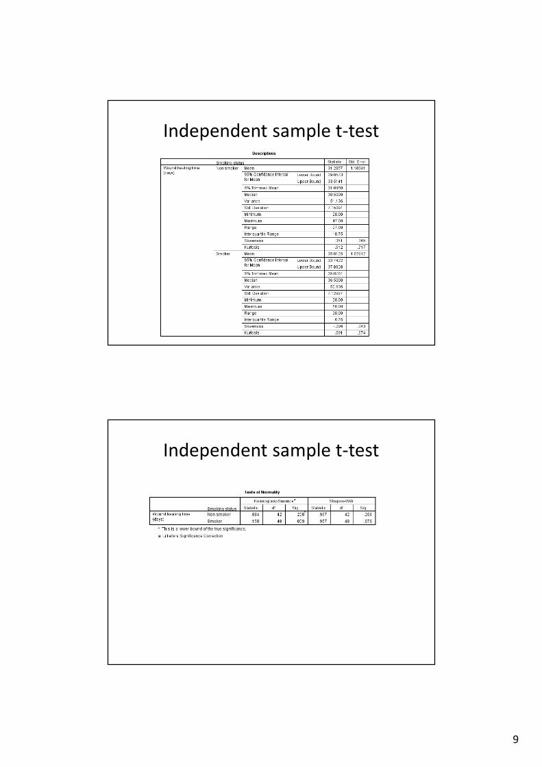
Step 3: check the assumptions
• Check normality : statistically and graphically
SPSS analyse Descriptive Explore
9
Independent sample t-test
Independent sample t-test

10
Independent sample t-test
Independent sample t-test
Step 3: check the assumptions
• Check homogeneity of variance Levene’stest

11
Independent sample t-test
Step 4: perform the SPSS analysis
Independent sample t-test
Step 4: perform the SPSS analysis
Assumption 5: Homogeneity of variance Test statistics. If equal variance assumed, read the upper row.

12
Independent sample t-test
Step 5: Interpret and make conclusion
• Mean (SD) wound healing among non-smoker = 31.29 (7.15)
• Mean (SD) wound healing among smoker = 35.82 (7.13)
• t-statistics=-3.00, df=88, P=0.004
• Mean difference = -4.53
• 95% CI of difference =-7.52, -1.53
Independent sample t-test
Step 5: Interpret and make conclusion
• Since the 95% CI does not cross 0, the P-value must be significant
• In this case, P=0.004
• Conclusion: Reject null hypothesis

13
Independent sample t-test
Step 6: Presentation of results.
• In text:
– The difference between mean (SD) of wound healing between non-smokers and smokers was statistically significant [31.29 (7.15) vs. 35.82 (7.13), P=0.004]
Independent sample t-test
Step 6: Presentation of results.
• In table:
Table 1: Comparison of wound healing time (days) between non-smokers and smokers
Variable Mean (SD) Mean diff. (95% CI) t-statistics (df)
P-value*
Smoker (n=42)
Non-smoker (n=48)
Wound healing (days)
31.29 (7.15)
35.82 (7.13)
-4.53 (-7.52, -1.53)
-3.00 (88)
0.004
*Independent sample t-test

14
PAIRED SAMPLE T-TEST
Paired sample t-test
• Also known as a dependent sample t-test
• A parametric test
• Used to compare two dependent or related samples
– Same subject, measure twice or repeatedly
– Matched study design
– Closely related subjects (e.g. twin studies)

15
Paired sample t-test
Same subject, measure twice
Study participants
Intervention group
HbA1c at baseline
HbA1c at 3/12
Control group
HbA1c at baseline
HbA1c at 3/12
compare
Paired sample t-test
Matched study design
Study participants
Intervention group
HbA1c at baseline
HbA1c at 3/12
Control group
HbA1c at baseline
HbA1c at 3/12
compare
Matched for age
16
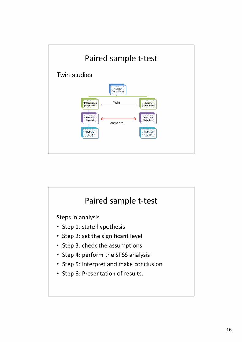
Paired sample t-test
Twin studies
Study participants
Intervention group: twin 1
HbA1c at baseline
HbA1c at 3/12
Control group: twin 2
HbA1c at baseline
HbA1c at 3/12
compare
Twin
Paired sample t-test
Steps in analysis
• Step 1: state hypothesis
• Step 2: set the significant level
• Step 3: check the assumptions
• Step 4: perform the SPSS analysis
• Step 5: Interpret and make conclusion
• Step 6: Presentation of results.

17
Paired sample t-test
Step 1: state hypothesis
• Null hypothesis
– Satisfaction pre = Satisfaction post
– µpre = µpost
• Alternative hypothesis
– Satisfaction pre Satisfaction post
– µpre µpost
Paired sample t-test
Step 2: set the significant level
• =0.05
• The acceptable level in medical and health sciences

18
Paired sample t-test
Step 3: check the assumptions1. Random samples (samples are
representative of the population)
2. The groups or measurements are dependent of each other
3. The outcome (dependent) variable is numerical data (interval or ratio)
4. The difference of outcome variable is normally distributed
Paired sample t-test
Step 3: check the assumptions
Study participants
Intervention group
HbA1c at baseline
HbA1c at 3/12
Control group
HbA1c at baseline
HbA1c at 3/12

19
Paired sample t-test
Step 3: check the assumptions
• To check normality of the difference, must compute the difference between pre and post
Paired sample t-test
Step 3: check the assumptions
• Then check histogram of the difference

20
Paired sample t-test
Step 3: check the assumptions
• Then check histogram of the difference
Paired sample t-test
Step 4: perform the SPSS analysis

21
Paired sample t-test
Step 4: perform the SPSS analysis
Paired sample t-test
Step 5: Interpret and make conclusion
• Mean (SD) of customer satisfaction pre = 37.46 (11.89)
• Mean (SD) of customer satisfaction post = 75.25 (16.36)
• Mean difference = 37.79
• 95% CI of difference = 33.59, 41.98
• t-statistics=17.93, df=79, P<0.001

22
Paired sample t-test
Step 5: Interpret and make conclusion
• Since the 95% CI does not cross 0, the P-value must be significant
• In this case, P<0.001
• Conclusion: Reject null hypothesis
Paired sample t-test
Step 6: Presentation of results.
• In text:
– The difference between mean (SD) of customer satisfaction before and after campaign started was statistically significant [37.46 (11.89) vs. 75.25 (16.36), P<0.001]

23
Paired sample t-test
Step 6: Presentation of results.
• In table:
Table 1: Comparison of customer satisfaction before and after campaign started
Variables measurement, Mean (SD) mean difference
(95% CI)
t-statistics
(df)
P-value*
Pre Post
Customer Satisfaction
Score 37.46 (11.89) 75.25 (16.36) 37.79 (33.59 ,41.98) 17.93 (79) <0.001
*Paired sample t-test
ONE WAY ANOVA

24
One way ANOVA
• Analysis of variance
• Compare mean of > two group
Study participants
Group A
BMI
Group B
BMI
Group C
BMI
One way ANOVA
• Comparison using multiple independent t-test inflates type I error
Study participants
Group A
BMI
Group B
BMI
Group C
BMI

25
One way ANOVA
• Commonly used to;
– Compare baseline characteristics among patients randomized into different treatment groups
– Compare post treatment differences between treatment groups
One way ANOVA
• Types of data:
1 independent variable (factor),• categorical • > two groups.Example: group A, B, C
1 dependent (outcome) variable• NumericalExample: BMI, SBP
One Way

26
One way ANOVA
Steps in analysis
• Step 1: state hypothesis
• Step 2: set the significant level
• Step 3: check the assumptions
• Step 4: perform the SPSS analysis
• Step 5: Interpret and make conclusion
• Step 6: Presentation of results.
One way ANOVA
Step 1: state hypothesis
• Null hypothesis
– There is no difference in mean recovery time between patients in three different treatment groups
– µa = µb = µc
• Alternative hypothesis
– At least one treatment group has a mean recovery time differ to another treatment group
– µa ≠ µb ≠ µc

27
One way ANOVA
Step 2: set the significant level
• =0.05
• The acceptable level in medical and health sciences
One way ANOVA
Step 3: check the assumptions1. Random samples (samples are representative of
the population)2. The groups and measurements are independent
of each other3. The outcome (dependent) variable is numerical
data (interval or ratio)4. The outcome variable is normally distributed
within each groups5. The variance between groups is approximately
equal (Homogeneity of variances)

28
One way ANOVA
Step 3: check the assumptions
Study participants
Group A
BMI
Group B
BMI
Group C
BMI
One way ANOVA
Step 3: check the assumptions
• The first three assumptions are determined by the study design
• The fourth must be checked before analysis. If violated, a non parametric test or data transformation will be needed.
• If the fifth assumption is violated, adjustment to the test must be made

29
One way ANOVA
Step 3: check the assumptions
• Check normality : statistically and graphically
SPSS analyse Descriptive Explore
One way ANOVA

30
One way ANOVA
One way ANOVA

31
One way ANOVA
Step 3: check the assumptions
• Check homogeneity of variance Levene’stest
One way ANOVA
Step 4: perform the SPSS analysis

32
One way ANOVA
Step 4: perform the SPSS analysis
One way ANOVA
Step 4: perform the SPSS analysis

33
One way ANOVA
Step 4: perform the SPSS analysis
Levene’s test is not significant (P > .05). Equal variance is assumed
One way ANOVA
Step 4: perform the SPSS analysis
• Overall ANOVA test. If significant (P < 0.05), indicates at least one of the mean is different to one another
• To determine which pair has a different mean, must do post hoc test.

34
One way ANOVA
Step 4: perform the SPSS analysis
• Post hoc test– A procedure to determine which pair show
different in means
– Involves multiple pairwise comparisons to test the mean differences between each pair
– If equal variance assumed Bonferroni, Scheffe, Tukey tests
– If equal variance not assumed Dunnett’s C, Games-Howell
One way ANOVA
Step 4: perform the SPSS analysis
• Post hoc test

35
One way ANOVA
Step 4: perform the SPSS analysis
• Post hoc test
One way ANOVA
Step 5: Interpret and make conclusion
• Drug A: M=62.55, SD=27.02
• Drug B: M=68.16, SD=21.58
• Drug C: M=45.10, SD=27.92
• One way ANOVA test is significant (P = 0.018) suggesting that at least one pair of mean recovery time between patients in different treatment groups was significantly different.
• Conclusion: reject null hypothesis

36
One way ANOVA
Step 5: Interpret and make conclusion
• Post hoc analysis using Bonferroni’sprocedure;
– Drug A vs drug B: MD=-5.61, 95% CI include 0, P > 0.95
– Drug A vs. drug C: MD=17.45, 95% CI include 0, P=0.109
– Drug B vs. drug C: MD=23.06, 95% CI does not include 0, P=0.021
One way ANOVA
Step 6: Presentation of results.
• In text:– One way ANOVA analysis suggest that recovery time
differ significantly across the three drugs [f(2,58)=4.30, P=0.018]
– Post hoc analysis using Bonferroni’s procedure suggest that the mean of recovery time between patients given drug B and C differ significantly
– Mean recovery time of patients given drug C was significantly faster compared to patients given drug B (M=45.10, SD=27.92 vs. M=68.16, SD=21.58, P=0.021)

37
One way ANOVA
Step 6: Presentation of results.
• In table:
Table 1: Mean recovery time between patients give different type of drug
Type of drugs N Recovery time,
Mean (SD)
F-statistics (df) P-value*
Drug A 20 62.55 (27.02) 4.30 (2, 58) 0.018
Drug B 19 68.16 (21.58)
Drug C 20 45.10 (27.92)
*One way ANOVA test Post-hoc analysis using Bonferroni’s procedure indicates that only mean recovery time between patients given drug B and C differ significantly (P=0.021)
Recap
• Compare numerical outcome variable between groups
2 independent groups independent t-test
2 dependent groups paired t-test
>2 independent groups one way ANOVA