explorations in numerical analysis - apache2 ubuntu ... · explorations in numerical analysis ......
TRANSCRIPT
Explorations in Numerical Analysis
James V. Lambers and Amber C. Sumner
December 1, 2017

ii
Copyright by
James V. Lambers and Amber C. Sumner
2016
Preface
This book evolved from lecture notes written by James Lambers and used in undergraduate numeri-cal analysis courses at the University of California at Irvine, Stanford University and the Universityof Southern Mississippi. It is written for a year-long sequence of numerical analysis courses for ei-ther advanced undergraduate or beginning graduate students. Part II is suitable for a semester-longfirst course on numerical linear algebra.
The goal of this book is to introduce students to numerical analysis from both a theoreticaland practical perspective, in such a way that these two perspectives reinforce each other. It isnot assumed that the reader has prior programming experience. As mathematical concepts areintroduced, code is used to illustrate them. As algorithms are developed from these concepts, thereader is invited to traverse the path from pseudocode to code.
Coding examples throughout the book are written in Matlab. Matlab has been a vital toolthroughout the numerical analysis community since its creation thirty years ago, and its syntax thatis oriented around vectors and matrices greatly accelerates the prototyping of algorithms comparedto other programming environments.
How to Use This Book
In order to get the most out of this book, it is recommended that you not simply read through it.As you have already seen, there are frequent “interruptions” in the text at which you are askedto perform some coding task. The purposes of these coding tasks are to get you accustomed toprogramming, particularly in Matlab, but also to reinforce the concepts of numerical analysis thatare presented throughout the book.
Reading about the design, analysis and implementation of the many algorithms covered inthis book is not sufficient to be able to fully understand these aspects or be able to efficientlyand effectively work with these algorithms in code, especially as part of a larger application. A“hands-on” approach is needed to achieve this level of proficiency, and this book is written withthis necessity in mind.
While the text is primarily intended for a one-year sequence in numerical analysis, naturallyinstructors will have their own priorities in terms of the depth and breadth with which the varioustopics are covered. With this in mind, sections or subsections that are considered optional aremarked with a * in the heading and in the Table of Contents. Furthermore, each section willindicate the sections on which it depends.
The first chapter includes a tutorial on Matlab. Depending on how much time the instructorhas, they can elect to have their students work through the entire tutorial at the beginning of
iii
iv
the first course, or defer coverage of certain sections until the relevant functions are needed–forexample, covering polynomial functions before polynomial interpolation in Chapter 6.
Appendices at the back of the book provide a thorough review of concepts from calculus andlinear algebra. It is recommended that students take time on their own to review these appendicesat the beginning of a first course. The dependence of sections within the main text on sections inthe appendices will also be indicated explicitly.
Acknowledgments
The authors would express their gratitude to Rochelle Kronzek and the very helpful and accom-modating staff at World Scientific for their assistance with and faith in this project. We are alsovery thankful for the feedback provided by anonymous reviewers on a draft. Finally, we are in-debted to the students in the authors’ MAT 460/560 and 461/561 courses, taught in 2015-16 andFall 2017, who were subjected to early drafts of this book. In particular, we would like to thankLaken Camp, Kaitlin Cooksey, Jade Dedeaux, Ross Grisham, Aaditya Kharel, Shiron Manandhar,Jesse Robinson, and Carley Walker for calling our attention to mistakes in the text and helping toimprove the clarity and quality of the explorations.
J. V. LambersA. C. Sumner
Contents
Contents v
List of Figures xi
List of Tables xiii
I Preliminaries 1
1 What is Numerical Analysis? 3
1.1 Overview . . . . . . . . . . . . . . . . . . . . . . . . . . . . . . . . . . . . . . . . . . 3
1.1.1 Error Analysis . . . . . . . . . . . . . . . . . . . . . . . . . . . . . . . . . . . 4
1.1.2 Systems of Linear Equations . . . . . . . . . . . . . . . . . . . . . . . . . . . 5
1.1.3 Polynomial Interpolation and Approximation . . . . . . . . . . . . . . . . . . 6
1.1.4 Numerical Differentiation and Integration . . . . . . . . . . . . . . . . . . . . 6
1.1.5 Nonlinear Equations . . . . . . . . . . . . . . . . . . . . . . . . . . . . . . . . 8
1.1.6 Optimization . . . . . . . . . . . . . . . . . . . . . . . . . . . . . . . . . . . . 8
1.1.7 Initial Value Problems . . . . . . . . . . . . . . . . . . . . . . . . . . . . . . . 9
1.1.8 Boundary Value Problems . . . . . . . . . . . . . . . . . . . . . . . . . . . . . 9
1.1.9 Partial Differential Equations . . . . . . . . . . . . . . . . . . . . . . . . . . . 10
1.2 Getting Started with MATLAB . . . . . . . . . . . . . . . . . . . . . . . . . . . . . 10
1.2.1 Obtaining Help . . . . . . . . . . . . . . . . . . . . . . . . . . . . . . . . . . . 10
1.2.2 Basic Mathematical Operations . . . . . . . . . . . . . . . . . . . . . . . . . . 11
1.2.3 Basic Matrix Operations . . . . . . . . . . . . . . . . . . . . . . . . . . . . . . 12
1.2.4 Storage of Variables . . . . . . . . . . . . . . . . . . . . . . . . . . . . . . . . 13
1.2.5 Complex Numbers . . . . . . . . . . . . . . . . . . . . . . . . . . . . . . . . . 14
1.2.6 Creating Special Vectors and Matrices . . . . . . . . . . . . . . . . . . . . . . 14
1.2.7 Suppressing Output . . . . . . . . . . . . . . . . . . . . . . . . . . . . . . . . 15
1.2.8 Building Matrices . . . . . . . . . . . . . . . . . . . . . . . . . . . . . . . . . 16
1.2.9 Accessing and Changing Entries of Matrices . . . . . . . . . . . . . . . . . . . 17
1.2.10 Transpose Operators . . . . . . . . . . . . . . . . . . . . . . . . . . . . . . . . 18
1.2.11 Conditional Expressions . . . . . . . . . . . . . . . . . . . . . . . . . . . . . . 19
1.2.12 if Statements . . . . . . . . . . . . . . . . . . . . . . . . . . . . . . . . . . . 20
1.2.13 for Loops . . . . . . . . . . . . . . . . . . . . . . . . . . . . . . . . . . . . . . 23
1.2.14 while Loops . . . . . . . . . . . . . . . . . . . . . . . . . . . . . . . . . . . . 26
v

vi CONTENTS
1.2.15 Function M-files . . . . . . . . . . . . . . . . . . . . . . . . . . . . . . . . . . 28
1.2.16 Graphics . . . . . . . . . . . . . . . . . . . . . . . . . . . . . . . . . . . . . . 31
1.2.17 Polynomial Functions . . . . . . . . . . . . . . . . . . . . . . . . . . . . . . . 32
1.2.18 Number Formatting . . . . . . . . . . . . . . . . . . . . . . . . . . . . . . . . 34
1.2.19 Inline and Anonymous Functions . . . . . . . . . . . . . . . . . . . . . . . . . 34
1.2.20 Other Helpful Functions . . . . . . . . . . . . . . . . . . . . . . . . . . . . . . 35
1.2.21 Saving and Loading Data . . . . . . . . . . . . . . . . . . . . . . . . . . . . . 36
1.2.22 Using Octave . . . . . . . . . . . . . . . . . . . . . . . . . . . . . . . . . . . . 36
1.3 Additional Resources . . . . . . . . . . . . . . . . . . . . . . . . . . . . . . . . . . . . 36
2 Approximation in Numerical Analysis 37
2.1 Error Analysis . . . . . . . . . . . . . . . . . . . . . . . . . . . . . . . . . . . . . . . 37
2.1.1 Sources of Approximation . . . . . . . . . . . . . . . . . . . . . . . . . . . . . 37
2.1.2 Error Measurement . . . . . . . . . . . . . . . . . . . . . . . . . . . . . . . . . 38
2.1.3 Forward and Backward Error . . . . . . . . . . . . . . . . . . . . . . . . . . . 40
2.1.4 Conditioning and Stability . . . . . . . . . . . . . . . . . . . . . . . . . . . . 41
2.1.5 Convergence . . . . . . . . . . . . . . . . . . . . . . . . . . . . . . . . . . . . 44
2.1.6 Concept Check . . . . . . . . . . . . . . . . . . . . . . . . . . . . . . . . . . . 49
2.2 Computer Arithmetic . . . . . . . . . . . . . . . . . . . . . . . . . . . . . . . . . . . 49
2.2.1 Floating-Point Representation . . . . . . . . . . . . . . . . . . . . . . . . . . . 50
2.2.2 Issues with Floating-Point Arithmetic . . . . . . . . . . . . . . . . . . . . . . 57
2.2.3 Concept Check . . . . . . . . . . . . . . . . . . . . . . . . . . . . . . . . . . . 60
2.3 Additional Resources . . . . . . . . . . . . . . . . . . . . . . . . . . . . . . . . . . . . 61
2.4 Exercises . . . . . . . . . . . . . . . . . . . . . . . . . . . . . . . . . . . . . . . . . . 61
III Data Fitting and Function Approximation 65
6 Polynomial Interpolation 67
6.1 Existence and Uniqueness . . . . . . . . . . . . . . . . . . . . . . . . . . . . . . . . . 67
6.1.1 Concept Check . . . . . . . . . . . . . . . . . . . . . . . . . . . . . . . . . . . 68
6.2 Lagrange Interpolation . . . . . . . . . . . . . . . . . . . . . . . . . . . . . . . . . . . 69
6.2.1 Lagrange Polynomials . . . . . . . . . . . . . . . . . . . . . . . . . . . . . . . 69
6.2.2 Barycentric Interpolation . . . . . . . . . . . . . . . . . . . . . . . . . . . . . 72
6.2.3 Concept Check . . . . . . . . . . . . . . . . . . . . . . . . . . . . . . . . . . . 73
6.3 Divided Differences . . . . . . . . . . . . . . . . . . . . . . . . . . . . . . . . . . . . . 73
6.3.1 Newton Form . . . . . . . . . . . . . . . . . . . . . . . . . . . . . . . . . . . . 75
6.3.2 Computing the Newton Interpolating Polynomial . . . . . . . . . . . . . . . . 76
6.3.3 Equally Spaced Points . . . . . . . . . . . . . . . . . . . . . . . . . . . . . . . 83
6.3.4 Concept Check . . . . . . . . . . . . . . . . . . . . . . . . . . . . . . . . . . . 86
6.4 Error Analysis . . . . . . . . . . . . . . . . . . . . . . . . . . . . . . . . . . . . . . . 86
6.4.1 Error Estimation . . . . . . . . . . . . . . . . . . . . . . . . . . . . . . . . . . 86
6.4.2 Chebyshev Interpolation . . . . . . . . . . . . . . . . . . . . . . . . . . . . . . 88
6.4.3 Concept Check . . . . . . . . . . . . . . . . . . . . . . . . . . . . . . . . . . . 90
6.5 Osculatory Interpolation . . . . . . . . . . . . . . . . . . . . . . . . . . . . . . . . . . 90
CONTENTS vii
6.5.1 Hermite Interpolation . . . . . . . . . . . . . . . . . . . . . . . . . . . . . . . 91
6.5.2 Divided Differences . . . . . . . . . . . . . . . . . . . . . . . . . . . . . . . . . 92
6.5.3 Concept Check . . . . . . . . . . . . . . . . . . . . . . . . . . . . . . . . . . . 94
6.6 Piecewise Polynomial Interpolation . . . . . . . . . . . . . . . . . . . . . . . . . . . . 95
6.6.1 Piecewise Linear Approximation . . . . . . . . . . . . . . . . . . . . . . . . . 95
6.6.2 Cubic Spline Interpolation . . . . . . . . . . . . . . . . . . . . . . . . . . . . . 97
6.6.3 Concept Check . . . . . . . . . . . . . . . . . . . . . . . . . . . . . . . . . . . 104
6.7 Additional Resources . . . . . . . . . . . . . . . . . . . . . . . . . . . . . . . . . . . . 105
6.8 Exercises . . . . . . . . . . . . . . . . . . . . . . . . . . . . . . . . . . . . . . . . . . 105
8 Differentiation and Integration 107
8.1 Numerical Differentiation . . . . . . . . . . . . . . . . . . . . . . . . . . . . . . . . . 107
8.1.1 Derivation Using Taylor Series . . . . . . . . . . . . . . . . . . . . . . . . . . 107
8.1.2 Derivation Using Lagrange Interpolation . . . . . . . . . . . . . . . . . . . . . 110
8.1.3 Higher-Order Derivatives . . . . . . . . . . . . . . . . . . . . . . . . . . . . . 113
8.1.4 Sensitivity . . . . . . . . . . . . . . . . . . . . . . . . . . . . . . . . . . . . . . 114
8.1.5 Differentiation Matrices . . . . . . . . . . . . . . . . . . . . . . . . . . . . . . 115
8.1.6 Concept Check . . . . . . . . . . . . . . . . . . . . . . . . . . . . . . . . . . . 116
8.2 Numerical Integration . . . . . . . . . . . . . . . . . . . . . . . . . . . . . . . . . . . 116
8.2.1 Quadrature Rules . . . . . . . . . . . . . . . . . . . . . . . . . . . . . . . . . 116
8.2.2 Interpolatory Quadrature . . . . . . . . . . . . . . . . . . . . . . . . . . . . . 117
8.2.3 Sensitivity . . . . . . . . . . . . . . . . . . . . . . . . . . . . . . . . . . . . . . 118
8.2.4 Concept Check . . . . . . . . . . . . . . . . . . . . . . . . . . . . . . . . . . . 119
8.3 Newton-Cotes Rules . . . . . . . . . . . . . . . . . . . . . . . . . . . . . . . . . . . . 119
8.3.1 Error Analysis . . . . . . . . . . . . . . . . . . . . . . . . . . . . . . . . . . . 121
8.3.2 Higher-Order Rules . . . . . . . . . . . . . . . . . . . . . . . . . . . . . . . . 122
8.3.3 Concept Check . . . . . . . . . . . . . . . . . . . . . . . . . . . . . . . . . . . 123
8.4 Composite Rules . . . . . . . . . . . . . . . . . . . . . . . . . . . . . . . . . . . . . . 123
8.4.1 Error Analysis . . . . . . . . . . . . . . . . . . . . . . . . . . . . . . . . . . . 124
8.4.2 Concept Check . . . . . . . . . . . . . . . . . . . . . . . . . . . . . . . . . . . 126
8.5 Gauss Quadrature . . . . . . . . . . . . . . . . . . . . . . . . . . . . . . . . . . . . . 126
8.5.1 Direct Construction . . . . . . . . . . . . . . . . . . . . . . . . . . . . . . . . 126
8.5.2 Orthogonal Polynomials . . . . . . . . . . . . . . . . . . . . . . . . . . . . . . 127
8.5.3 Error Analysis . . . . . . . . . . . . . . . . . . . . . . . . . . . . . . . . . . . 128
8.5.4 Other Weight Functions . . . . . . . . . . . . . . . . . . . . . . . . . . . . . . 132
8.5.5 Prescribing Nodes . . . . . . . . . . . . . . . . . . . . . . . . . . . . . . . . . 133
8.5.6 Concept Check . . . . . . . . . . . . . . . . . . . . . . . . . . . . . . . . . . . 135
8.6 Extrapolation to the Limit . . . . . . . . . . . . . . . . . . . . . . . . . . . . . . . . . 135
8.6.1 Richardson Extrapolation . . . . . . . . . . . . . . . . . . . . . . . . . . . . . 136
8.6.2 The Euler-Maclaurin Expansion . . . . . . . . . . . . . . . . . . . . . . . . . 137
8.6.3 Romberg Integration . . . . . . . . . . . . . . . . . . . . . . . . . . . . . . . . 139
8.6.4 Concept Check . . . . . . . . . . . . . . . . . . . . . . . . . . . . . . . . . . . 142
8.7 Adaptive Quadrature . . . . . . . . . . . . . . . . . . . . . . . . . . . . . . . . . . . . 143
8.7.1 Concept Check . . . . . . . . . . . . . . . . . . . . . . . . . . . . . . . . . . . 149
8.8 Multiple Integrals . . . . . . . . . . . . . . . . . . . . . . . . . . . . . . . . . . . . . . 149
viii CONTENTS
8.8.1 Double Integrals . . . . . . . . . . . . . . . . . . . . . . . . . . . . . . . . . . 149
8.8.2 Higher Dimensions . . . . . . . . . . . . . . . . . . . . . . . . . . . . . . . . . 153
8.8.3 Concept Check . . . . . . . . . . . . . . . . . . . . . . . . . . . . . . . . . . . 154
8.9 Additional Resources . . . . . . . . . . . . . . . . . . . . . . . . . . . . . . . . . . . . 154
8.10 Exercises . . . . . . . . . . . . . . . . . . . . . . . . . . . . . . . . . . . . . . . . . . 155
IV Appendices 159
A Review of Calculus 161
A.1 Limits and Continuity . . . . . . . . . . . . . . . . . . . . . . . . . . . . . . . . . . . 161
A.1.1 Limits . . . . . . . . . . . . . . . . . . . . . . . . . . . . . . . . . . . . . . . . 161
A.1.2 Limits of Functions of Several Variables . . . . . . . . . . . . . . . . . . . . . 163
A.1.3 Limits at Infinity . . . . . . . . . . . . . . . . . . . . . . . . . . . . . . . . . . 164
A.1.4 Continuity . . . . . . . . . . . . . . . . . . . . . . . . . . . . . . . . . . . . . 164
A.1.5 The Intermediate Value Theorem . . . . . . . . . . . . . . . . . . . . . . . . . 165
A.2 Derivatives . . . . . . . . . . . . . . . . . . . . . . . . . . . . . . . . . . . . . . . . . 166
A.2.1 Differentiability and Continuity . . . . . . . . . . . . . . . . . . . . . . . . . . 167
A.3 Extreme Values . . . . . . . . . . . . . . . . . . . . . . . . . . . . . . . . . . . . . . . 167
A.4 Integrals . . . . . . . . . . . . . . . . . . . . . . . . . . . . . . . . . . . . . . . . . . . 169
A.5 The Mean Value Theorem . . . . . . . . . . . . . . . . . . . . . . . . . . . . . . . . . 170
A.5.1 The Mean Value Theorem for Integrals . . . . . . . . . . . . . . . . . . . . . 171
A.6 Taylor’s Theorem . . . . . . . . . . . . . . . . . . . . . . . . . . . . . . . . . . . . . . 172
B Review of Linear Algebra 177
B.1 Matrices . . . . . . . . . . . . . . . . . . . . . . . . . . . . . . . . . . . . . . . . . . . 177
B.2 Vector Spaces . . . . . . . . . . . . . . . . . . . . . . . . . . . . . . . . . . . . . . . . 177
B.3 Subspaces . . . . . . . . . . . . . . . . . . . . . . . . . . . . . . . . . . . . . . . . . . 179
B.4 Linear Independence and Bases . . . . . . . . . . . . . . . . . . . . . . . . . . . . . . 179
B.5 Linear Transformations . . . . . . . . . . . . . . . . . . . . . . . . . . . . . . . . . . 181
B.5.1 The Matrix of a Linear Transformation . . . . . . . . . . . . . . . . . . . . . 182
B.5.2 Matrix-Vector Multiplication . . . . . . . . . . . . . . . . . . . . . . . . . . . 182
B.5.3 Special Subspaces . . . . . . . . . . . . . . . . . . . . . . . . . . . . . . . . . 183
B.6 Matrix-Matrix Multiplication . . . . . . . . . . . . . . . . . . . . . . . . . . . . . . . 183
B.7 Other Fundamental Matrix Operations . . . . . . . . . . . . . . . . . . . . . . . . . . 185
B.7.1 Vector Space Operations . . . . . . . . . . . . . . . . . . . . . . . . . . . . . . 185
B.7.2 The Transpose of a Matrix . . . . . . . . . . . . . . . . . . . . . . . . . . . . 185
B.7.3 Inner and Outer Products . . . . . . . . . . . . . . . . . . . . . . . . . . . . . 186
B.7.4 Hadamard Product . . . . . . . . . . . . . . . . . . . . . . . . . . . . . . . . . 188
B.7.5 Partitioning . . . . . . . . . . . . . . . . . . . . . . . . . . . . . . . . . . . . . 188
B.8 Understanding Matrix-Matrix Multiplication . . . . . . . . . . . . . . . . . . . . . . 189
B.8.1 The Identity Matrix . . . . . . . . . . . . . . . . . . . . . . . . . . . . . . . . 189
B.8.2 The Inverse of a Matrix . . . . . . . . . . . . . . . . . . . . . . . . . . . . . . 190
B.9 Triangular and Diagonal Matrices . . . . . . . . . . . . . . . . . . . . . . . . . . . . . 190
B.10 Determinants . . . . . . . . . . . . . . . . . . . . . . . . . . . . . . . . . . . . . . . . 191

CONTENTS ix
B.11 Eigenvalues . . . . . . . . . . . . . . . . . . . . . . . . . . . . . . . . . . . . . . . . . 193B.12 Vector and Matrix Norms . . . . . . . . . . . . . . . . . . . . . . . . . . . . . . . . . 194
B.12.1 Vector Norms . . . . . . . . . . . . . . . . . . . . . . . . . . . . . . . . . . . . 194B.12.2 Matrix Norms . . . . . . . . . . . . . . . . . . . . . . . . . . . . . . . . . . . . 196B.12.3 Function Spaces and Norms . . . . . . . . . . . . . . . . . . . . . . . . . . . . 199
B.13 Inner Product Spaces . . . . . . . . . . . . . . . . . . . . . . . . . . . . . . . . . . . . 200B.14 Convergence . . . . . . . . . . . . . . . . . . . . . . . . . . . . . . . . . . . . . . . . . 201B.15 Differentiation of Matrices . . . . . . . . . . . . . . . . . . . . . . . . . . . . . . . . . 203
Bibliography 205
Index 217

x CONTENTS
List of Figures
1.1 The dotted red curves demonstrate polynomial interpolation (left plot) and least-squares approximation (right plot) applied to f(x) = 1/(1 + x2) (blue solid curve). . 7
1.2 Screen shot of Matlab at startup in Mac OS X . . . . . . . . . . . . . . . . . . . . 111.3 Figure for Exploration 1.2.20 . . . . . . . . . . . . . . . . . . . . . . . . . . . . . . . 33
6.1 The function f(x) = 1/(1 + x2) (solid curve) cannot be interpolated accurately on[−5, 5] using a tenth-degree polynomial (dashed curve) with equally-spaced interpo-lation points. . . . . . . . . . . . . . . . . . . . . . . . . . . . . . . . . . . . . . . . . 88
6.2 Cubic spline that passing through the points (0, 3), (1/2,−4), (1, 5), (2,−6), and (3, 7).101
8.1 Graph of f(x) = e3x sin 2x on [0, π/4], with quadrature nodes from Example 8.7.2shown on the graph and on the x-axis. . . . . . . . . . . . . . . . . . . . . . . . . . . 148
xi

xii LIST OF FIGURES

List of Tables
xiii

xiv LIST OF TABLES

Part I
Preliminaries
1

Chapter 1
What is Numerical Analysis?
1.1 Overview
This book provides a comprehensive introduction to the subject of numerical analysis, which isthe study of the design, analysis, and implementation of numerical algorithms for solving mathe-matical problems that arise in science and engineering. These numerical algorithms differ from theanalytical methods that are presented in other mathematics courses, in that they rely exclusivelyon the four basic arithmetic operations–addition, subtraction, multiplication and division–so thatthey can be implemented on a computer. As such, numerical analysis, a branch of mathematics,is an essential component of scientific computing, also known as computational science, which isa multidisciplinary field devoted to the solution of problems in science and engineering throughcomputing technology.
Numerical analysis is employed to develop and analyze algorithms for solving problems thatarise in other areas of mathematics, such as calculus, linear algebra, or differential equations. Ofcourse, these areas already include algorithms for solving such problems, but these algorithms areanalytical methods. Examples of analytical methods are:
• Applying the Fundamental Theorem of Calculus to evaluate a definite integral,
• Using Gaussian elimination, with exact arithmetic, to solve a system of linear equations, and
• Using the method of undetermined coefficients to solve an inhomogeneous ordinary differentialequation.
Such analytical methods have the benefit that they yield exact solutions, but the drawback is thatthey can only be applied to a limited range of problems. Numerical methods, on the other hand, canbe applied to a much wider range of problems, but only yield approximate solutions. Fortunately, inmany applications, one does not necessarily need very high accuracy, and even when such accuracyis required, it can still be obtained, if one is willing to expend the extra computational effort (or,really, have a computer do so).
The goal in numerical analysis is to develop numerical methods that are effective, in terms ofthe following criteria:
• A numerical method must be accurate. While this seems like common sense, careful consid-eration must be given to the notion of accuracy. For a given problem, what level of accuracy
3
4 CHAPTER 1. WHAT IS NUMERICAL ANALYSIS?
is considered sufficient? As will be discussed in Section 2.1, there are many sources of error.As such, it is important to question whether it is prudent to expend resources to reduce onetype of error, when another type of error is already more significant. This will be illustratedin Section 8.1.
• A numerical method must be efficient. Although computing power has been rapidly increasingin recent decades, this has resulted in expectations of solving larger-scale problems. Therefore,it is essential that numerical methods produce approximate solutions with as few arithmeticoperations or data movements as possible. Efficiency is not only important in terms of time;memory is still a finite resource and therefore algorithms must also aim to minimize datastorage needs.
• A numerical method must be robust. A method that is highly accurate and efficient for some(or even most) problems, but performs poorly on others, is unreliable and therefore not likelyto be used in applications, even if any alternative is not as accurate and efficient. The userof a numerical method needs to know that the result produced can be trusted.
These criteria should be balanced according to the requirements of the application. For example,if less accuracy is acceptable, then greater efficiency can be achieved. This can be the case, forexample, if there is so much uncertainty in the underlying mathematical model that there is nopoint in obtaining high accuracy.
In this section, we provide an overview of the topics that will be covered in this book. Whilethis selection of topics is not intended to be an exhaustive list of topics that could be covered in anundergraduate sequence, it does provide the reader with a sufficiently broad and deep backgroundto pursue further study through more advanced coursework or research.
1.1.1 Error Analysis
Because solutions produced by numerical algorithms are not exact, we will begin our exploration ofnumerical analysis with one of its most fundamental concepts, which is error analysis. Numericalalgorithms must not only be efficient, but they must also be accurate, and robust. In other words,the solutions they produce are at best approximate solutions because an exact solution cannotbe computed by analytical techniques. Furthermore, these computed solutions should not be toosensitive to the input data, because if they are, any error in the input can result in a solution thatis essentially useless. Such error can arise from many sources, such as
• neglecting components of a mathematical model or making simplifying assumptions in themodel,
• discretization error, which arises from approximating continuous functions by sets of discretedata points,
• convergence error, which arises from truncating a sequence of approximations that is meantto converge to the exact solution, to make computation possible, and
• roundoff error, which is due to the fact that computers represent real numbers approximately,in a fixed amount of storage in memory.
1.1. OVERVIEW 5
We will see that in some cases, these errors can be surprisingly large, so one must be carefulwhen designing and implementing numerical algorithms. Section 2.1 will introduce fundamentalconcepts of error analysis that will be used throughout this book, and Section 2.2 will discusscomputer arithmetic and roundoff error in detail.
1.1.2 Systems of Linear Equations
Next, we will learn about how to solve a system of linear equations
a11x1 + a12x2 + · · ·+ a1nxn = b1
a21x1 + a22x2 + · · ·+ a2nxn = b2...
an1x1 + an2x2 + · · ·+ annxn = bn,
which can be more conveniently written in matrix-vector form
Ax = b,
where A is an n× n matrix, because the system has n equations (corresponding to rows of A) andn unknowns (corresponding to columns).
To solve a general system with n equations and unknowns, we can use Gaussian eliminationto reduce the system to upper-triangular form, which is easy to solve. In some cases, this processrequires pivoting, which entails interchanging of rows or columns of the matrix A. Gaussian elimi-nation with pivoting can be used not only to solve a system of equations, but also to compute theinverse of a matrix, even though this is not normally practical. It can also be used to efficientlycompute the determinant of a matrix.
Gaussian elimination with pivoting can be viewed as a process of factorizing the matrix A.Specifically, it achieves the decomposition
PA = LU,
where P is a permutation matrix that describes any row interchanges, L is a lower-triangularmatrix, and U is an upper-triangular matrix. This decomposition, called the LU decomposition, isparticularly useful for solving Ax = b when the right-hand side vector b varies. We will see thatfor certain special types of matrices, such as those that arise in the normal equations, variations ofthe general approach to solving Ax = b can lead to improved efficiency.
Gaussian elimination and related methods are called direct methods for solving Ax = b, becausethey compute the exact solution (up to roundoff error, which can be significant in some cases) ina fixed number of operations that depends on n. However, such methods are often not practical,especially when A is very large, or when it is sparse, meaning that most of its entries are equal tozero. Therefore, we also consider iterative methods. Two general classes of iterative methods are:
• stationary iterative methods, which can be viewed as fixed-point iterations, and rely primarilyon splittings of A to obtain a system of equations that can be solved rapidly in each iteration,and
6 CHAPTER 1. WHAT IS NUMERICAL ANALYSIS?
• non-stationary methods, which tend to rely on matrix-vector multiplication in each iterationand a judicious choice of search direction and linesearch to compute each iterate from theprevious one.
We will also consider systems of equations, for which the number of equations, m, is greaterthan the number of unknowns, n. This is the least-squares problem, which is reduced to a systemwith n equations and unknowns,
ATAx = ATb,
called the normal equations. While this system can be solved directly using methods discussedabove, this can be problematic due to sensitivity to roundoff error. We therefore explore otherapproaches based on orthogonalization of the columns of A.
Another fundamental problem from linear algebra is the solution of the eigenvalue problem
Ax = λx,
where the scalar λ is called an eigenvalue and the nonzero vector x is called an eigenvector. Thisproblem has many applications throughout applied mathematics, including the solution of differen-tial equations and statistics. We will see that the tools developed for efficient and robust solutionof least squares problems are useful for the eigenvalue problem as well.
1.1.3 Polynomial Interpolation and Approximation
Polynomials are among the easiest functions to work with, because it is possible to evaluate them,as well as perform operations from calculus on them, with great efficiency. For this reason, morecomplicated functions, or functions that are represented only by values on a discrete set of pointsin their domain, are often approximated by polynomials.
Such an approximation can be computed in various ways. We first consider interpolation,in which we construct a polynomial that agrees with the given data at selected points. Whileinterpolation methods are efficient, they must be used carefully, because it is not necessarily truethat a polynomial that agrees with a given function at certain points is a good approximation tothe function elsewhere in its domain.
One remedy for this is to use piecewise polynomial interpolation, in which a low-degree polyno-mial, typically linear or cubic, is used to approximate data only on a given subdomain, and thesepolynomial “pieces” are “glued” together to obtain a piecewise polynomial approximation. Thisapproach is also efficient, and tends to be more robust than standard polynomial interpolation, butthere are disadvantages, such as the fact that a piecewise polynomial only has very few derivatives.
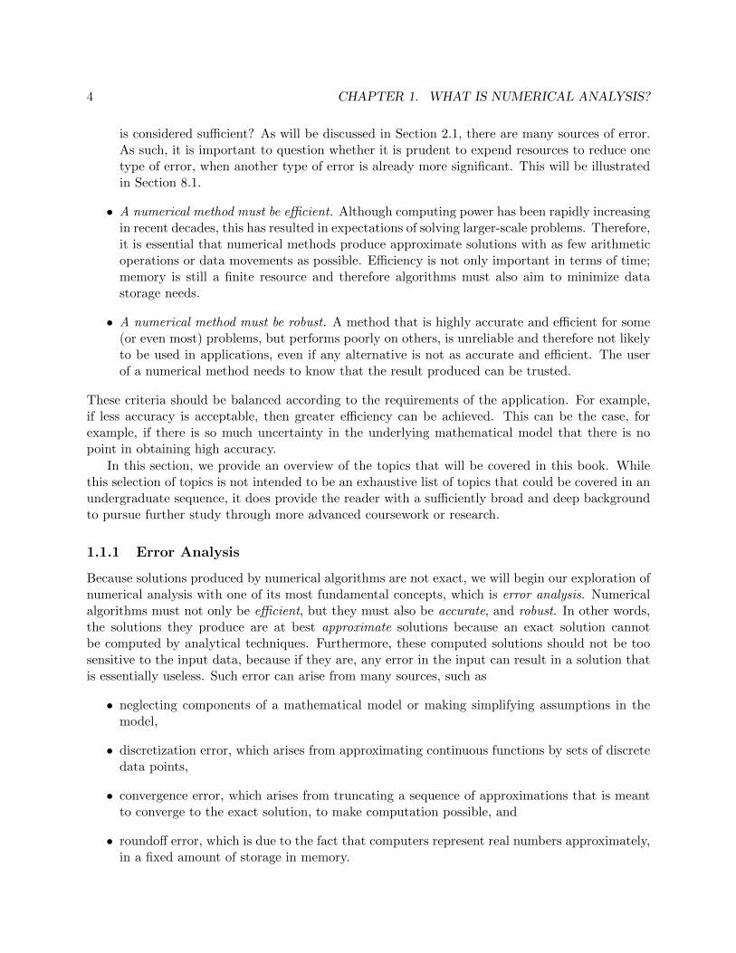
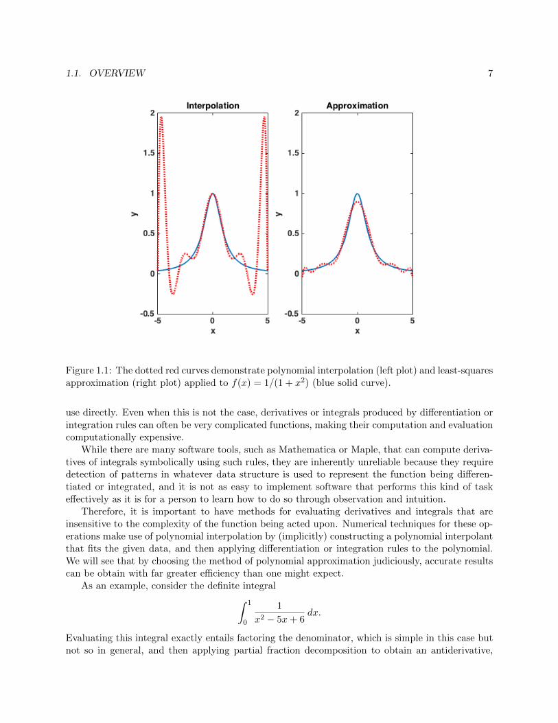
An alternative to polynomial interpolation, whether piecewise or not, is polynomial approxi-mation, in which the goal is to find a polynomial that, in some sense, best fits given data. Forexample, it is not possible to exactly fit a large number of points with a low-degree polynomial,but an approximate fit can be more useful than a polynomial that can fit the given data exactlybut still fail to capture the overall behavior of the data. This is illustrated in Figure 1.1.
1.1.4 Numerical Differentiation and Integration
It is often necessary to approximate derivatives or integrals of functions that are represented onlyby values at a discrete set of points, thus making differentiation or integration rules impossible to
1.1. OVERVIEW 7
Figure 1.1: The dotted red curves demonstrate polynomial interpolation (left plot) and least-squaresapproximation (right plot) applied to f(x) = 1/(1 + x2) (blue solid curve).
use directly. Even when this is not the case, derivatives or integrals produced by differentiation orintegration rules can often be very complicated functions, making their computation and evaluationcomputationally expensive.
While there are many software tools, such as Mathematica or Maple, that can compute deriva-tives of integrals symbolically using such rules, they are inherently unreliable because they requiredetection of patterns in whatever data structure is used to represent the function being differen-tiated or integrated, and it is not as easy to implement software that performs this kind of taskeffectively as it is for a person to learn how to do so through observation and intuition.
Therefore, it is important to have methods for evaluating derivatives and integrals that areinsensitive to the complexity of the function being acted upon. Numerical techniques for these op-erations make use of polynomial interpolation by (implicitly) constructing a polynomial interpolantthat fits the given data, and then applying differentiation or integration rules to the polynomial.We will see that by choosing the method of polynomial approximation judiciously, accurate resultscan be obtain with far greater efficiency than one might expect.
As an example, consider the definite integral∫ 1
0
1
x2 − 5x+ 6dx.
Evaluating this integral exactly entails factoring the denominator, which is simple in this case butnot so in general, and then applying partial fraction decomposition to obtain an antiderivative,

8 CHAPTER 1. WHAT IS NUMERICAL ANALYSIS?
which is then evaluated at the limits. Alternatively, simply computing
1
12[f(0) + 4f(1/4) + 2f(1/2) + 4f(3/4) + f(1)],
where f(x) is the integrand, yields an approximation with 0.01% error (that is, the error is 10−4).While the former approach is less tedious to carry out by hand, at least if one has a calculator,clearly the latter approach is the far more practical use of computational resources.
1.1.5 Nonlinear Equations
The vast majority of equations, especially nonlinear equations, cannot be solved using analyticaltechniques such as algebraic manipulations or knowledge of trigonometric functions. For example,while the equations
x2 − 5x+ 6 = 0, cosx =1
2
can easily be solved to obtain exact solutions, these slightly different equations
x2 − 5xex + 6 = 0, x cosx =1
2
cannot be solved using analytical methods.
Therefore, iterative methods must instead be used to obtain an approximate solution. We willstudy a variety of such methods, which have distinct advantages and disadvantages. For example,some methods are guaranteed to produce a solution under reasonable assumptions, but they mightdo so slowly. On the other hand, other methods may produce a sequence of iterates that quicklyconverges to the solution, but may be unreliable for some problems.
After learning how to solve nonlinear equations of the form f(x) = 0 using iterative methodssuch as Newton’s method, we will learn how to generalize such methods to solve systems of nonlinearequations of the form f(x) = 0, where f : Rn → Rn. In particular, for Newton’s method, computingxn+1 − xn = −f(xn)/f ′(xn) in the single-variable case is generalized to solving the system ofequations Jf (xn)sn = −f(xn), where Jf (xn) is the Jacobian of f evaluated at xn, and sn =xn+1 − xn is the step from each iterate to the next.
1.1.6 Optimization
We then turn our attention to the very important problem of optimization, in which we seekto minimize or maximize a given function, known as an objective function. Our exploration ofoptimization begins with relatively simple techniques that do not require any information aboutderivatives of the objective function. It will be seen that these techniques have natural analoguesto methods for solving nonlinear equations.
Such methods for solution of nonlinear equations play an essential role in optimization tech-niques that require finding critical points of the objective function, as the derivative or gradientof the objective function is equal to zero at such points. We will examine a variety of methodsbased on this simple idea, as designing an efficient and robust algorithm for optimization is farfrom simple.

1.1. OVERVIEW 9
1.1.7 Initial Value Problems
Next, we study various algorithms for solving an initial value problem, which consists of an ordinarydifferential equation (ODE)
dy
dt= f(t, y), a ≤ t ≤ b,
an initial condition
y(t0) = α.
Unlike analytical methods for solving such problems, that are used to find the exact solution in theform of a function y(t), numerical methods typically compute values y1, y2, y3, . . . that approximatey(t) at discrete time values t1, t2, t3, . . .. At each time tn+1, for n > 0, value of the solution isapproximated using its values at previous times.
We will learn about two general classes of methods: one-step methods, which are derived usingTaylor series and compute yn+1 only from yn, and multistep methods, which are based on polynomialinterpolation and compute yn+1 from yn, yn−1, . . . , yn−s+1, where s is the number of steps in themethod. Either type of method can be explicit, in which yn+1 can be described in terms of anexplicit formula, or implicit, in which yn+1 is described implicitly using an equation, normallynonlinear, that must be solved during each time step.
The difference between consecutive times tn and tn+1, called the time step, need not be uniform;we will learn about how it can be varied to achieve a desired level of accuracy as efficiently aspossible. We will also learn about how the methods used for the first-order initial-value problemdescribed above can be generalized to solve higher-order equations, as well as systems of equations.
One key issue with time-stepping methods is stability. If the time step is not chosen to besufficiently small, the computed solution can grow without bound, even if the exact solution isbounded. Generally, the need for stability imposes a more severe restriction on the size of the timestep for explicit methods, which is why implicit methods are commonly used, even though theytend to require more computational effort per time step. Certain systems of differential equationscan require an extraordinarily small time step to be solved by explicit methods; such systems aresaid to be stiff.
1.1.8 Boundary Value Problems
We then discuss solution methods for the two-point boundary value problem
y′′ = f(x, y, y′), a ≤ x ≤ b,
with boundary conditions
y(a) = α, y(b) = β.
One approach, called the shooting method, transforms this boundary-value problem into an initial-value problem so that methods for such problems can then be used. However, it is necessary tofind the correct initial values so that the boundary condition at x = b is satisfied. An alternativeapproach is to discretize y′′ and y′ using finite differences, the approximation schemes covered inChapter 8, to obtain a system of equations to solve for an approximation of y(x); this system canbe linear or nonlinear. We conclude with the finite element method, which treats the boundaryvalue problem as a continuous least-squares problem.
10 CHAPTER 1. WHAT IS NUMERICAL ANALYSIS?
1.1.9 Partial Differential Equations
We conclude the book with an introduction to numerical methods for the solution of partial dif-ferential equations (PDEs). Techniques for two-point boundary value problems are generalized tohigher spatial dimensions for the purpose of solving equations such as Laplace’s equation. For time-dependent PDEs, such as the heat equation or the wave equation, techniques for boundary-valueproblems are combined with time-stepping techniques for initial value problems.
In Chapter ??, we first examine finite-difference methods, similar to those used for boundary-value problems, except applied to all partial derivatives with respect to both spatial and temporalvariables. Then, we provide an introduction to the finite element method, that is more conduciveto solving PDEs on non-rectangular domains.
1.2 Getting Started with MATLAB
Matlab is commercial software, originally developed by Cleve Moler in 1982 [131] and currentlysold by The Mathworks. It can be purchased and downloaded from mathworks.com. As of thiswriting, the student version can be obtained for $50, whereas academic and industrial licenses aremuch more expensive. For any license, “toolboxes” can be purchased in order to obtain additionalfunctionality, but for the tasks performed in this book, the core product will be sufficient.
As an alternative, one can instead use Octave, a free application which uses the same program-ming language as Matlab, with only minor differences. It can be obtained from gnu.org. Itsuser interface is not as “friendly” as that of Matlab, but it has improved significantly in its mostrecent versions. In this book, examples will feature only Matlab, but the code will also work inOctave, without modification except where noted.
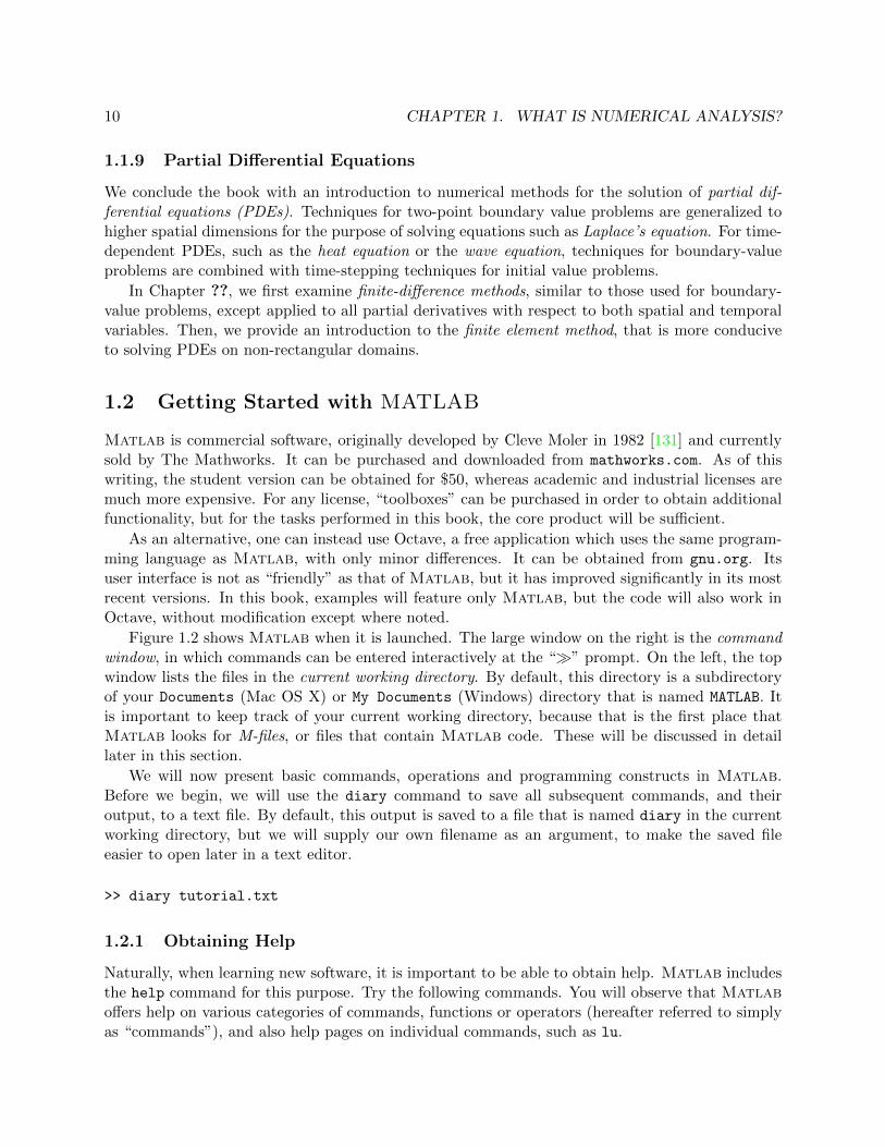
Figure 1.2 shows Matlab when it is launched. The large window on the right is the commandwindow, in which commands can be entered interactively at the “” prompt. On the left, the topwindow lists the files in the current working directory. By default, this directory is a subdirectoryof your Documents (Mac OS X) or My Documents (Windows) directory that is named MATLAB. Itis important to keep track of your current working directory, because that is the first place thatMatlab looks for M-files, or files that contain Matlab code. These will be discussed in detaillater in this section.
We will now present basic commands, operations and programming constructs in Matlab.Before we begin, we will use the diary command to save all subsequent commands, and theiroutput, to a text file. By default, this output is saved to a file that is named diary in the currentworking directory, but we will supply our own filename as an argument, to make the saved fileeasier to open later in a text editor.
>> diary tutorial.txt
1.2.1 Obtaining Help
Naturally, when learning new software, it is important to be able to obtain help. Matlab includesthe help command for this purpose. Try the following commands. You will observe that Matlaboffers help on various categories of commands, functions or operators (hereafter referred to simplyas “commands”), and also help pages on individual commands, such as lu.
1.2. GETTING STARTED WITH MATLAB 11
Figure 1.2: Screen shot of Matlab at startup in Mac OS X
>> help
>> help ops
>> help lu
1.2.2 Basic Mathematical Operations
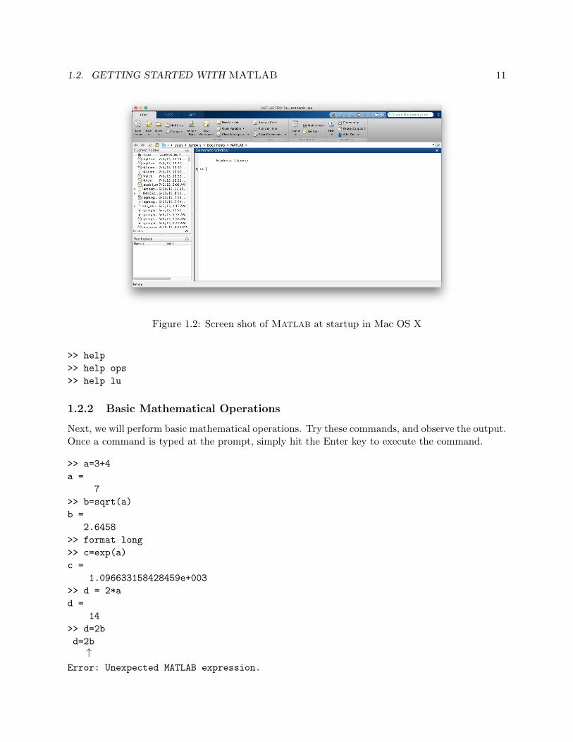
Next, we will perform basic mathematical operations. Try these commands, and observe the output.Once a command is typed at the prompt, simply hit the Enter key to execute the command.
>> a=3+4
a =
7
>> b=sqrt(a)
b =
2.6458
>> format long
>> c=exp(a)
c =
1.096633158428459e+003
>> d = 2*a
d =
14
>> d=2b
d=2b↑
Error: Unexpected MATLAB expression.
12 CHAPTER 1. WHAT IS NUMERICAL ANALYSIS?
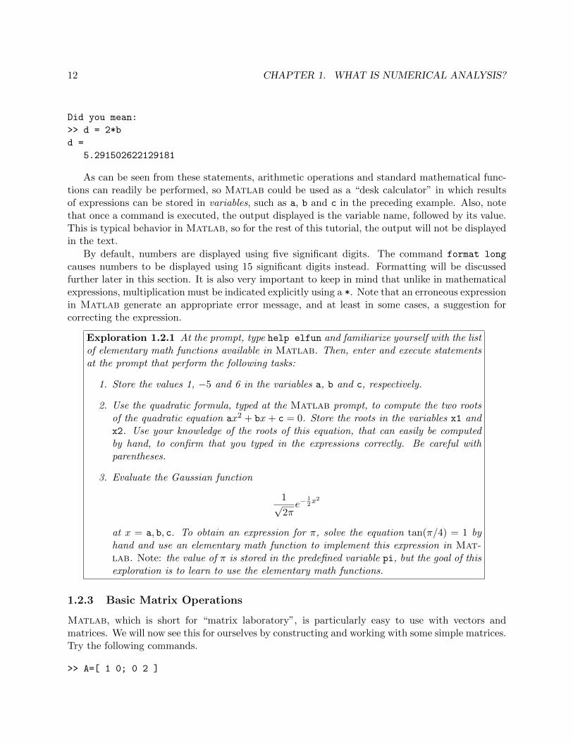
Did you mean:
>> d = 2*b
d =
5.291502622129181
As can be seen from these statements, arithmetic operations and standard mathematical func-tions can readily be performed, so Matlab could be used as a “desk calculator” in which resultsof expressions can be stored in variables, such as a, b and c in the preceding example. Also, notethat once a command is executed, the output displayed is the variable name, followed by its value.This is typical behavior in Matlab, so for the rest of this tutorial, the output will not be displayedin the text.
By default, numbers are displayed using five significant digits. The command format long
causes numbers to be displayed using 15 significant digits instead. Formatting will be discussedfurther later in this section. It is also very important to keep in mind that unlike in mathematicalexpressions, multiplication must be indicated explicitly using a *. Note that an erroneous expressionin Matlab generate an appropriate error message, and at least in some cases, a suggestion forcorrecting the expression.
Exploration 1.2.1 At the prompt, type help elfun and familiarize yourself with the listof elementary math functions available in Matlab. Then, enter and execute statementsat the prompt that perform the following tasks:
1. Store the values 1, −5 and 6 in the variables a, b and c, respectively.
2. Use the quadratic formula, typed at the Matlab prompt, to compute the two rootsof the quadratic equation ax2 + bx+ c = 0. Store the roots in the variables x1 andx2. Use your knowledge of the roots of this equation, that can easily be computedby hand, to confirm that you typed in the expressions correctly. Be careful withparentheses.
3. Evaluate the Gaussian function
1√2πe−
12x2
at x = a, b, c. To obtain an expression for π, solve the equation tan(π/4) = 1 byhand and use an elementary math function to implement this expression in Mat-lab. Note: the value of π is stored in the predefined variable pi, but the goal of thisexploration is to learn to use the elementary math functions.
1.2.3 Basic Matrix Operations
Matlab, which is short for “matrix laboratory”, is particularly easy to use with vectors andmatrices. We will now see this for ourselves by constructing and working with some simple matrices.Try the following commands.
>> A=[ 1 0; 0 2 ]
1.2. GETTING STARTED WITH MATLAB 13
>> B=[ 5 7; 9 10 ]
>> A+B
>> 2*ans
>> C=A+B
>> 4*A
>> C=A-B
>> C=A*B
>> w=[ 4; 5; 6 ]
As we can see, matrix arithmetic is easily performed. However, what happens if we attempt anoperation that, mathematically, does not make sense? Consider the following example, in which a2× 2 matrix is multiplied by a 3× 1 vector.
>> A*w
??? Error using ==> mtimes
Inner matrix dimensions must agree.
Since this operation is invalid, Matlab does not attempt to perform the operation and insteaddisplays an error message. The function name mtimes refers to the function that implements thematrix multiplication operator that is represented in the above command by *.
Exploration 1.2.2 Let
A =
2 −43 −57 0
, B =
−5 1 44 6 8
10 5 0
, C =
−8 02 −3−1 4
.Carry out the computation D = A+ 3BC by hand, and then use Matlab to check yourwork. Note: You may need to review Section B.6 about matrix-matrix multiplication andSection B.7.1 about matrix addition and scalar multiplication.
1.2.4 Storage of Variables
Let’s examine the variables that we have created so far (exclusive of any explorations). The whos
command is useful for this purpose.
>> whos
Name Size Bytes Class Attributes
A 2x2 32 double
B 2x2 32 double
C 2x2 32 double
a 1x1 8 double
ans 2x2 32 double
b 1x1 8 double
c 1x1 8 double
w 3x1 24 double

14 CHAPTER 1. WHAT IS NUMERICAL ANALYSIS?
Note that each number, such as a, or each entry of a matrix, occupies 8 bytes of storage, whichis the amount of memory allocated to a double-precision floating-point number. This system ofrepresenting real numbers will be discussed further in Section 2.2. Also, note the variable ans. Itwas not explicitly created by any of the commands that we have entered. It is a special variablethat is assigned the most recent expression that is not already assigned to a variable. In this case,the value of ans is the output of the operation 4*A, since that was not assigned to any variable.
1.2.5 Complex Numbers
Matlab can also work with complex numbers. The following command creates a vector with onereal element and one complex element.
>> z=[ 6; 3+4i ]
Now run the whos command again. Note that it states that z occupies 32 bytes, even though it hasonly two elements. This is because each element of z has a real part and an imaginary part, andeach part occupies 8 bytes. It is important to note that if a single element of a vector or matrix iscomplex, then the entire vector or matrix is considered complex. This can result in wasted storageif imaginary parts are supposed to be zero, but in fact are small, nonzero numbers due to roundofferror (which will be discussed in Section 2.2).
The real and imag commands can be used to extract the real and imaginary parts, respectively,of a complex scalar, vector or matrix. The output of these commands are stored as real numbers.
>> y=real(z)
>> y=imag(z)
Exploration 1.2.3 Use Matlab to compute the (complex) roots of the quadratic equa-tion x2 + 4x+ 9 = 0, as in Exploration 1.2.1, and then substitute them into the equationto verify the correctness of the roots.
Exploration 1.2.4 At the prompt, set the variable theta equal to a (radian) angle θ ofyour choosing. Then, form the complex number z = c+ is, where c = cos θ and s = sin θ.Compare to the result that you obtain by computing eiθ. Note: in place of i, use 1i forthe imaginary unit i =
√−1, as it is more efficient.
1.2.6 Creating Special Vectors and Matrices
It can be very tedious to create matrices entry-by-entry, as we have done so far. Fortunately,Matlab has several functions that can be used to easily create certain matrices of interest. Trythe following commands to learn what these functions do. In particular, note the behavior whenonly one argument is given, instead of two.
>> E=ones(6,5)
>> E=ones(3)
>> Z=zeros(3,4)
>> Z=zeros(1,6)
>> R=rand(3,2)
1.2. GETTING STARTED WITH MATLAB 15
As the names suggest, ones creates a matrix with all entries equal to one, zeros creates a matrixwith all entries equal to zero, and rand creates a matrix with random entries. More precisely, theentries are random numbers that are uniformly distributed on [0, 1].
Exploration 1.2.5 What if we want the entries of a matrix to be random numbers thatare distributed within a different interval, such as [−1, 1]? Create such a matrix, of size3× 2, using matrix arithmetic that we have seen, and the ones function.
In many situations, it is helpful to have a vector of equally spaced values. For example, if wewant a vector consisting of the integers from 1 to 10, inclusive, we can create it using the statement
>> z=[ 1 2 3 4 5 6 7 8 9 10 ]
However, this can be very tedious if a vector with many more entries is needed. Imagine creatinga vector with all of the integers from 1 to 1000! Fortunately, this can easily be accomplished usingthe colon operator. Try the following commands to see how this operator behaves.
>> z=1:10
>> z=1:2:10
>> z=10:-2:1
>> z=1:-2:10
It should be noted that the second argument, that determines spacing between entries, need notbe an integer.
Exploration 1.2.6 Use the colon operator to create a vector of real numbers between 0and 1, inclusive, with spacing 0.01.
Exploration 1.2.7 Use the help function to learn about the linspace function. Howwould you use this function to create the vectors 1:10, 1:2:10 or 1:0.01:10?
1.2.7 Suppressing Output
Suppose that we create a random 3× 3 matrix at the prompt. The output will look something likethis:
>> A=rand(3)
A =
0.5667 0.8350 0.0031
0.1063 0.5301 0.2453
0.0798 0.3264 0.0194
We see that the matrix is printed out. Now, try the same statement, but instead create a 50× 50matrix, or an even larger one. Needless to say, such a statement produces a substantial amount ofoutput.
16 CHAPTER 1. WHAT IS NUMERICAL ANALYSIS?
This is problematic for several reasons. First, such output may not be necessary, and thereforethe time spent producing it, which can be substantial, is wasted. Second, this output is notconducive to “user-friendliness” of an application built in Matlab. Fortunately, this output canbe suppressed by adding a semicolon to the end of the statement:
>> A=rand(50);
>>
In general, any statement that evaluates an arithmetic or logical expression produces output, if itis not concluded with a semicolon. Specifically, the value of any expression that is computed inthat statement is displayed, along with its variable name (or ans, if there is no variable associatedwith the expression). It is interesting to note that in Matlab, semicolons at the end of statementsare optional, unlike languages such as C, C++ or Java, in which they are required.
In most cases, suppressing output is the desired behavior, for the reasons given above. However,omitting semicolons can be useful when writing and debugging new code, because seeing interme-diate results of a computation can expose bugs. Once the code is working, then semicolons can beadded to suppress superfluous output.
1.2.8 Building Matrices
We have seen how to create matrices either entry-by-entry, as in Section 1.2.3, or with varioushelper functions, as in Section 1.2.6. Here, we demonstrate how to easily create smaller matricesthan larger ones. First, we create the following matrices:
>> A=[ 2 3; 1 4 ];
>> B=[ -1 4 5; 2 -6 7 ];
>> C=[ -1 1; 2 -3; 5 -4 ];
Now, try these statements:
>> X=[ A B ];
>> Y=[ A; C ];
We see that the first statement concatenates matrices horizontally, while the second concatenatesthem vertically.
Exploration 1.2.8 With the matrices A, B, C above, try these statements:
>> Z=[ A; B ];
>> W=[ A C ];
What happens with these statements? In general, when can matrices be concatenatedhorizontally, or vertically?
An empty matrix can be constructed using an empty pair of square brackets:
>> x=[]
Then, entries or matrices can be concatenated onto the empty matrix. For example, here is howwe can iteratively build up a row vector from “nothing”:
1.2. GETTING STARTED WITH MATLAB 17
>> x=[ x 1 ]
x =
1
>> x=[ x 2 ]
x =
1 2
>> x=[ x 2 3 4 5 ]
x =
1 2 3 4 5
How would the preceding statements be modified to build a column vector from an emptymatrix, rather than a row vector?
While this is a convenient way to iteratively build a matrix (or a vector, if there is only onerow or column), it is important to note that it is also inefficient, as the memory associated withthe matrix must be deallocated and then reallocated to make room for new entries. This addssubstantial overhead that can be avoided if the entire matrix is preallocated, once, using the zeros
function.
1.2.9 Accessing and Changing Entries of Matrices
Now that we know how to create matrices, we need to be able to work with individual entries ofmatrices, including accessing them and modifying them. Individual entries are accessed using thefollowing notation:
>> A=[ 2 3; 1 4 ];
>> A(1,2)
ans =
3
In general, aij is accessed using the syntax A(i,j). It’s important to note that Matlab using“1-based indexing”, meaning that the indices i and j must assume values in the ranges 1, 2, . . . ,mand 1, 2, . . . , n, respectively, where A is m× n. This contrasts with languages such as C++, whichuses 0-based indexing.
In many instances, it is helpful to be able to extract submatrices, such as a row, column, orblock. Try these statements and describe the portion of A that each one extracts:
>> A=rand(3)
>> A(1,1:3)
>> A(1:2,1)
>> A(1:2,1:2)
>> A(:,3)
>> A(1,:)
>> A(:,end)
>> A(2:end,1)

18 CHAPTER 1. WHAT IS NUMERICAL ANALYSIS?
>> A([ 1 3 ],:)
>> A(:,[ 3 2 ])
>> B=rand(5)
>> B([ 1 4 3 ],[ 5 2 ])
It can be seen from these statements that row vectors can be used as indices. That is, if A is m×n,and if p is a row vector of length k and q is a row vector of length l, where k ≤ m and l ≤ n, thenthe expression A(p,q) returns the k × l submatrix
ap1,q1 ap1,q2 · · · ap1,qlap2,q1 ap2,q2 · · · ap2,ql
......
apk,q1 apk,q2 · · · apk,ql
.Furthermore, using a : by itself in place of a row vector is a shorthand for all possible indices,which is convenient for extracting entire rows or columns. Finally, end, when used as an index,refers to the largest possible index.
Exploration 1.2.9 Given a matrix A, write a Matlab expression that represents A withits rows and columns both in reverse order, using the : operator.
Exploration 1.2.10 Given a matrix A, and two indices i and j, with i 6= j, write aMatlab statement that interchanges rows i and j of A (that is, the statement overwritesthese rows of A with the interchanged rows).
1.2.10 Transpose Operators
We now know how to create row vectors with equally spaced values, but what if we would ratherhave a column vector? This is just one of many instances in which we need to be able to computethe transpose of a matrix (see Section B.7.2) in Matlab. Fortunately, this is easily accomplished,using the single quote as an operator. For example, this statement
>> z=(0:0.1:1)’
has the desired effect. However, one should not simply conclude that the single quote is thetranspose operator, or they could be in for an unpleasant surprise when working with complex-valued matrices. Try these commands to see why:
>> z=[ 6; 3+4i ]
>> z’
>> z.’
We can see that the single quote is an operator that takes the Hermitian transpose of a matrixA, commonly denoted by AH : it is the transpose and complex conjugate of A. That is, AH = AT .Meanwhile, the dot followed by the single quote is the transpose operator.
Either operator can be used to take the transpose for matrices with real entries, but one mustbe more careful when working with complex entries. That said, why is the “default” behavior, rep-resented by the simpler single quote operator, the Hermitian transpose rather than the transpose?
1.2. GETTING STARTED WITH MATLAB 19
This is because in general, results or techniques established for real matrices, that make use of thetranspose, do not generalize to the complex case unless the Hermitian transpose is used instead.
Exploration 1.2.11 The `2-norm, or simply 2-norm, of a vector x ∈ Cn is definedin Section B.12.1 by ‖x‖2 =
√xHx. As ‖x‖2 must be a real, positive number for any
nonzero vector x, justify the definition by finding a nonzero vector x such that xTx, asopposed to xHx, is a) negative, b) zero, or c) imaginary.
1.2.11 Conditional Expressions
We have already learned about arithmetic operators such as + or *. Here, we learn about relationaland logical operators, which are featured in other programming languages as well. Help on theseoperators can be obtained by typing help ops at the prompt. The relational operators are:
== equal to~= not equal to< less than<= less than or equal to> greater than>= greater than or equal to
Note that the “not equal” operator is different than that used in other languages such as C++ orJava. Evaluate the following relational expressions at the prompt:
>> 4>3
ans =
logical
1
>> 1==0
ans =
logical
0
Note that the value of a conditional expression is 1 if the expression is true, and 0 if it is false. Alsonote that these values are considered to be of type logical, and therefore occupies only one byte,rather than the eight bytes occupied by a real number.
The logical operators are
&& short-circuit logical AND|| short-circuit logical OR& element-wise logical AND| element-wise logical OR~ logical NOT
The short-circuit operators can only be used with operands that are scalars (that is, not a vector ormatrix). Short-circuit evaluation is an efficient approach to evaluating expressions involving severalAND or OR operators. For example, x && y && z is false if x is false, in which case y and z arenot evaluated at all. Similarly, x || y || z is true if x is true, and again y and z are not evaluatedat all.
20 CHAPTER 1. WHAT IS NUMERICAL ANALYSIS?
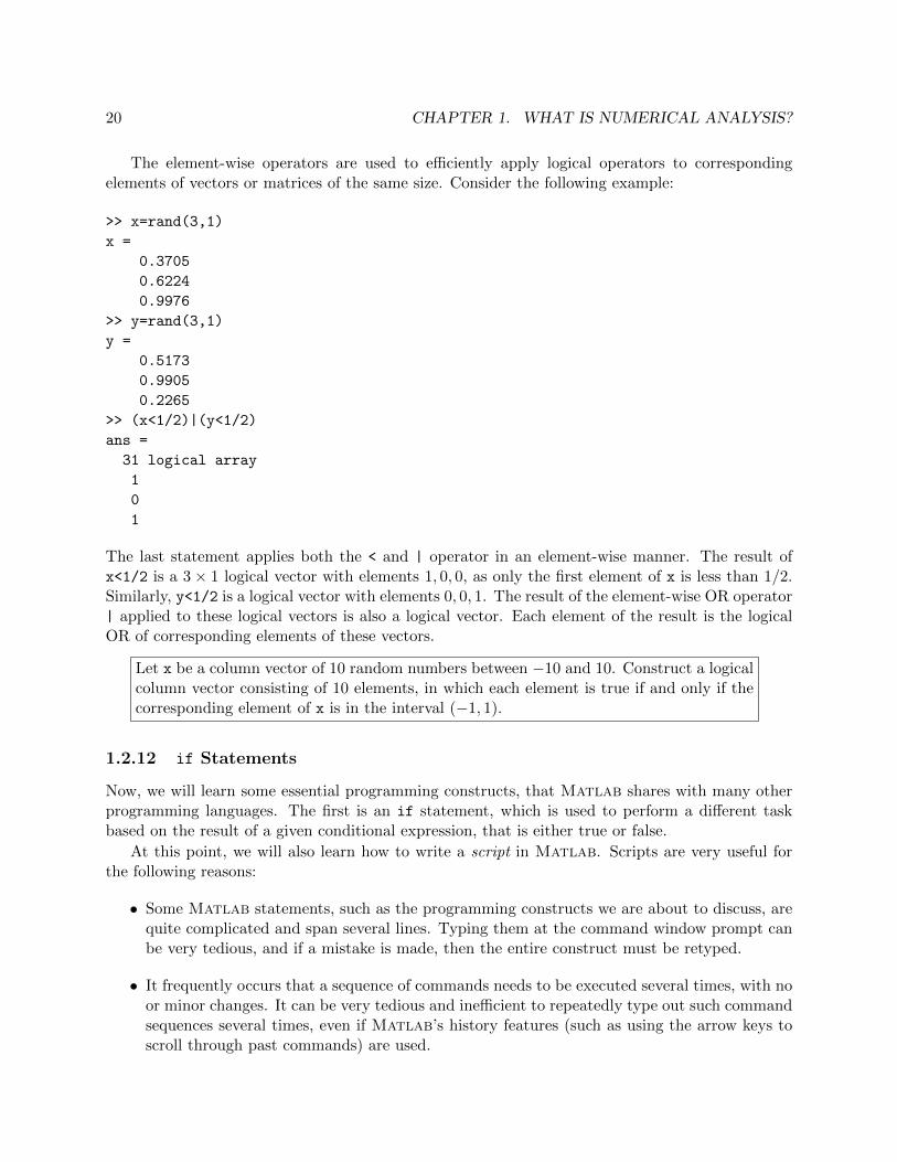
The element-wise operators are used to efficiently apply logical operators to correspondingelements of vectors or matrices of the same size. Consider the following example:
>> x=rand(3,1)
x =
0.3705
0.6224
0.9976
>> y=rand(3,1)
y =
0.5173
0.9905
0.2265
>> (x<1/2)|(y<1/2)
ans =
31 logical array
1
0
1
The last statement applies both the < and | operator in an element-wise manner. The result ofx<1/2 is a 3× 1 logical vector with elements 1, 0, 0, as only the first element of x is less than 1/2.Similarly, y<1/2 is a logical vector with elements 0, 0, 1. The result of the element-wise OR operator| applied to these logical vectors is also a logical vector. Each element of the result is the logicalOR of corresponding elements of these vectors.
Let x be a column vector of 10 random numbers between −10 and 10. Construct a logicalcolumn vector consisting of 10 elements, in which each element is true if and only if thecorresponding element of x is in the interval (−1, 1).
1.2.12 if Statements
Now, we will learn some essential programming constructs, that Matlab shares with many otherprogramming languages. The first is an if statement, which is used to perform a different taskbased on the result of a given conditional expression, that is either true or false.
At this point, we will also learn how to write a script in Matlab. Scripts are very useful forthe following reasons:
• Some Matlab statements, such as the programming constructs we are about to discuss, arequite complicated and span several lines. Typing them at the command window prompt canbe very tedious, and if a mistake is made, then the entire construct must be retyped.
• It frequently occurs that a sequence of commands needs to be executed several times, with noor minor changes. It can be very tedious and inefficient to repeatedly type out such commandsequences several times, even if Matlab’s history features (such as using the arrow keys toscroll through past commands) are used.

1.2. GETTING STARTED WITH MATLAB 21
A script can be written in a plain text file, called an M-file, which is a file that has a .m extension.An M-file can be written in any text editor, or in Matlab’s own built-in editor. To create a newM-file or edit an existing M-file, one can use the edit command at the prompt:
>> edit signofx
If no extension is given, a .m extension is assumed. If the file does not exist in the current workingdirectory or in Matlab’s search path, Matlab will ask if the file should be created.
In the editor, type in the following code, that displays an appropriate message according towhether the (numeric) value of a variable x is positive, negative, or zero.
x=2*rand(1)-1;
disp(x)
if x>0
disp(’x is positive’)
elseif x<0
disp(’x is negative’)
else
disp(’x is zero’)
end
When you save, the file signofx.m will be saved in the current directory. To execute a script M-file,simply type the name of the file (without the .m extension) at the prompt.
>> signofx
-0.8169
x is negative
The code in this script first assigns a value to x, and then displays this value using the disp
function. Note that the output produced by disp differs from statements that produce output dueto the lack of a semicolon, as only the value is displayed, not the name of the variable or an equalssign. For this reason, the use of disp is often the preferred approach to producing output, as theoutput can be given a more professional appearance. This will be illustrated in later examples.
Next, the conditional expression x<0 is evaluated. Then, the if statement containing thisconditional expression is executed according to the result of the evaluation. If the conditionalexpression is true, then the statements immediately following it are executed. In this example, thatmeans the statement disp(’x is positive’) would be executed.
Also note the use of the keywords else and elseif. These are used to provide alternativeconditions under which different code can be executed, if the original condition in the if statementturns out to be false. If any conditions paired with the elseif keyword also turn out to be false,then the code following the else keyword, if any, is executed. Finally, note that the entire if
statement is concluded with the end keyword.For a more advanced example, type the following code into the script file entermonthyear.m.
This code computes and displays the number of days in a given month, while taking leap years intoaccount. As this example demonstrates, if statements can be nested within one another.
% entermonthyear - script that asks the user to provide a month and year,
% and displays the number of days in that month
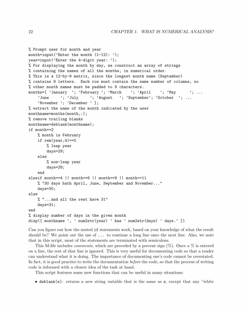
22 CHAPTER 1. WHAT IS NUMERICAL ANALYSIS?
% Prompt user for month and year
month=input(’Enter the month (1-12): ’);
year=input(’Enter the 4-digit year: ’);
% For displaying the month by day, we construct an array of strings
% containing the names of all the months, in numerical order.
% This is a 12-by-9 matrix, since the longest month name (September)
% contains 9 letters. Each row must contain the same number of columns, so
% other month names must be padded to 9 characters.
months=[ ’January ’; ’February ’; ’March ’; ’April ’; ’May ’; ...
’June ’; ’July ’; ’August ’; ’September’; ’October ’; ...
’November ’; ’December ’ ];
% extract the name of the month indicated by the user
monthname=months(month,:);
% remove trailing blanks
monthname=deblank(monthname);
if month==2
% month is February
if rem(year,4)==0
% leap year
days=29;
else
% non-leap year
days=28;
end
elseif month==4 || month==6 || month==9 || month==11
% "30 days hath April, June, September and November..."
days=30;
else
% "...and all the rest have 31"
days=31;
end
% display number of days in the given month
disp([ monthname ’, ’ num2str(year) ’ has ’ num2str(days) ’ days.’ ])
Can you figure out how the nested if statements work, based on your knowledge of what the resultshould be? We point out the use of ... to continue a long line onto the next line. Also, we notethat in this script, most of the statements are terminated with semicolons.
This M-file includes comments, which are preceded by a percent sign (%). Once a % is enteredon a line, the rest of that line is ignored. This is very useful for documenting code so that a readercan understand what it is doing. The importance of documenting one’s code cannot be overstated.In fact, it is good practice to write the documentation before the code, so that the process of writingcode is informed with a clearer idea of the task at hand.
This script features some new functions that can be useful in many situations:
• deblank(s): returns a new string variable that is the same as s, except that any “white
1.2. GETTING STARTED WITH MATLAB 23
space” (spaces, tabs, or newlines) at the end of s is removed
• rem(a,b): returns the remainder after dividing a by b
• num2str(x): returns a string variable based on formatting the number x as text
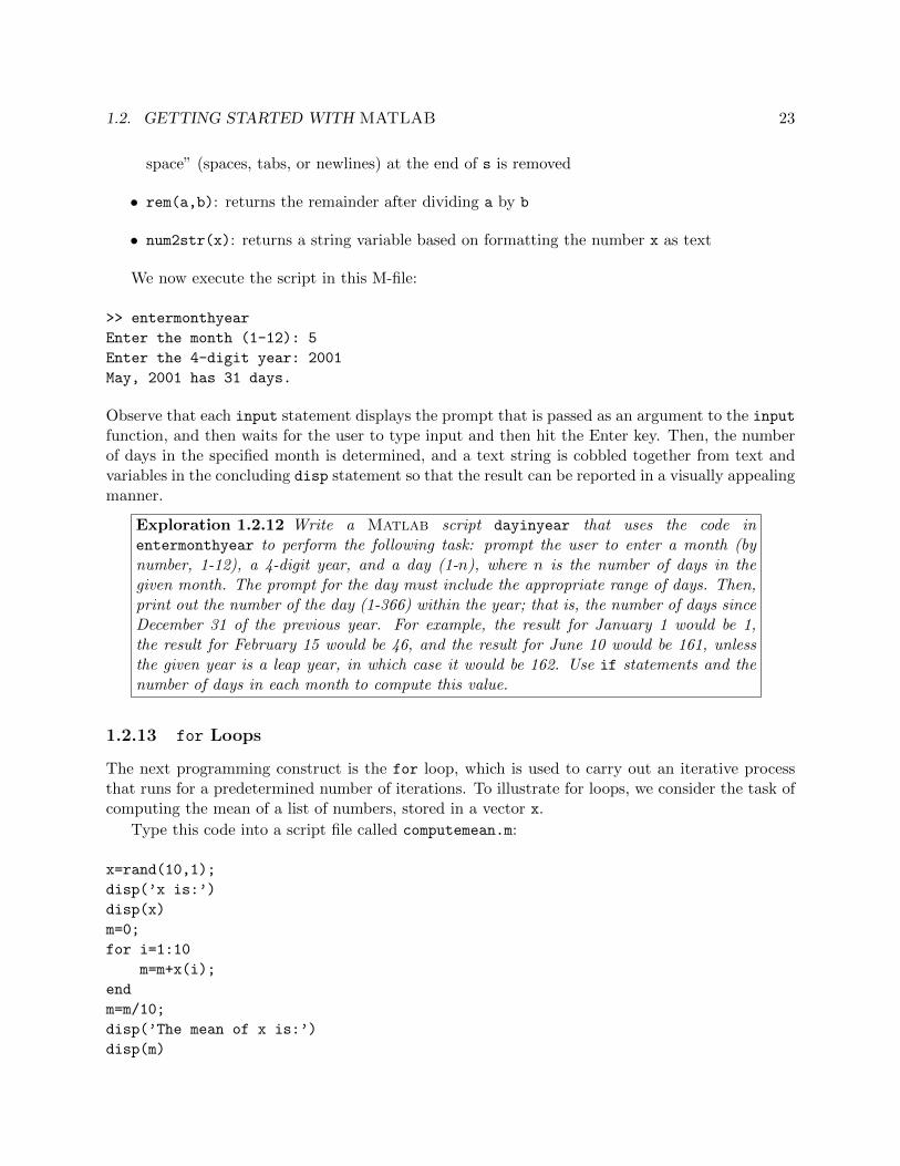
We now execute the script in this M-file:
>> entermonthyear
Enter the month (1-12): 5
Enter the 4-digit year: 2001
May, 2001 has 31 days.
Observe that each input statement displays the prompt that is passed as an argument to the inputfunction, and then waits for the user to type input and then hit the Enter key. Then, the numberof days in the specified month is determined, and a text string is cobbled together from text andvariables in the concluding disp statement so that the result can be reported in a visually appealingmanner.
Exploration 1.2.12 Write a Matlab script dayinyear that uses the code inentermonthyear to perform the following task: prompt the user to enter a month (bynumber, 1-12), a 4-digit year, and a day (1-n), where n is the number of days in thegiven month. The prompt for the day must include the appropriate range of days. Then,print out the number of the day (1-366) within the year; that is, the number of days sinceDecember 31 of the previous year. For example, the result for January 1 would be 1,the result for February 15 would be 46, and the result for June 10 would be 161, unlessthe given year is a leap year, in which case it would be 162. Use if statements and thenumber of days in each month to compute this value.
1.2.13 for Loops
The next programming construct is the for loop, which is used to carry out an iterative processthat runs for a predetermined number of iterations. To illustrate for loops, we consider the task ofcomputing the mean of a list of numbers, stored in a vector x.
Type this code into a script file called computemean.m:
x=rand(10,1);
disp(’x is:’)
disp(x)
m=0;
for i=1:10
m=m+x(i);
end
m=m/10;
disp(’The mean of x is:’)
disp(m)

24 CHAPTER 1. WHAT IS NUMERICAL ANALYSIS?
Since the vector x has 10 elements, the mean of the elements of x is given by the formula
m =1
10
10∑i=1
xi.
To “count from 1 to 10” in the process of accessing all of the elements of x for the purpose of addingthem, we use a for statement.
Now run this script, just like in the previous example.
>> computemean
x is:
0.3148
0.7267
0.5158
0.7906
0.2045
0.6781
0.0525
0.8012
0.6786
0.9460
The mean of x is:
0.5709
The loop performed 10 iterations to compute the sum of the elements x, which is approximately5.7088.
Note the syntax for a for statement: the keyword for is followed by a loop variable, such asi in the preceding example, and that variable is assigned a value. Then the body of the loop isgiven, followed by the keyword end.
What does a for loop actually do? During the ith iteration, the loop variable i is set equal tothe ith column of the expression that is assigned to it by the for statement. Then, the loop variableretains this value throughout the body of the loop (unless the loop variable is changed within thebody of the loop, which is ill-advised, and sometimes done by mistake!), until the iteration iscompleted. Then, the loop variable is assigned the next column for the next iteration. In mostcases, such as in this example, the loop variable is simply used as a counter, in which case assigningto it a row vector of values, created using the colon operator, yields the desired behavior.
Modify the script computemean.m to write a new script computevariance.m that com-putes the (population) variance of x:
v =1
10
10∑i=1
(xi − m)2.
For our next example, we use an if statement inside a for statement. The following scriptcomputes the maximum of a list of numbers, again stored in a vector x. We will call this scriptfindmax.m:
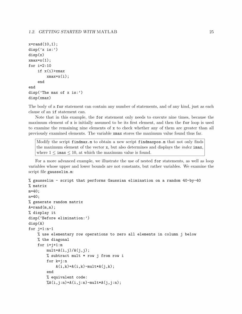
1.2. GETTING STARTED WITH MATLAB 25
x=rand(10,1);
disp(’x is:’)
disp(x)
xmax=x(1);
for i=2:10
if x(i)>xmax
xmax=x(i);
end
end
disp(’The max of x is:’)
disp(xmax)
The body of a for statement can contain any number of statements, and of any kind, just as eachclause of an if statement can.
Note that in this example, the for statement only needs to execute nine times, because themaximum element of x is initially assumed to be its first element, and then the for loop is usedto examine the remaining nine elements of x to check whether any of them are greater than allpreviously examined elements. The variable xmax stores the maximum value found thus far.
Modify the script findmax.m to obtain a new script findmaxpos.m that not only findsthe maximum element of the vector x, but also determines and displays the index imax,where 1 ≤ imax ≤ 10, at which the maximum value is found.
For a more advanced example, we illustrate the use of nested for statements, as well as loopvariables whose upper and lower bounds are not constants, but rather variables. We examine thescript file gausselim.m:
% gausselim - script that performs Gaussian elimination on a random 40-by-40
% matrix
m=40;
n=40;
% generate random matrix
A=rand(m,n);
% display it
disp(’Before elimination:’)
disp(A)
for j=1:n-1
% use elementary row operations to zero all elements in column j below
% the diagonal
for i=j+1:m
mult=A(i,j)/A(j,j);
% subtract mult * row j from row i
for k=j:n
A(i,k)=A(i,k)-mult*A(j,k);
end
% equivalent code:
%A(i,j:n)=A(i,j:n)-mult*A(j,j:n);
26 CHAPTER 1. WHAT IS NUMERICAL ANALYSIS?
end
end
% display updated matrix
disp(’After elimination:’)
disp(A)
The script displays a randomly generated matrix A, then performs Gaussian elimination on A toobtain an upper triangular matrix, and then displays the final result. Note that while the outermostloop, with loop variable j, executes n − 1 times, where the matrix A is m × n, the next innermostloop, with loop variable j, executes m−j times, due to the variable starting value of j+1. Similarly,the innermost loop, with loop variable k, executes n− j + 1 times.
Note the commented-out statement A(i,j:n) = A(i,j:n) - mult*A(j,j:n). This statementcan be used instead of the innermost for loop that begins with for k=j:n. This is because eachiteration of this loop does not depend on the result of previous iterations, so the relevant portion(columns j through n) of the jth row of A, scaled by mult, can be subtracted from the same portionof the ith row of A in a single operation. In other words, this statement is an implicit for loop,because it must still be carried out through an iteration, but that iteration is implied by the rangeof indices j:n.
Exploration 1.2.13 An upper triangular matrix U has the property that uij = 0 when-ever i > j; that is, the entire “lower triangle” of U , consisting of all entries below themain diagonal, must be zero (see Section B.9). Examine the matrix A produced by thescript gausselim above. Why are some subdiagonal entries nonzero?
Exploration 1.2.14 Write a script matadd that creates two m × n matrices A and B,and uses for loops to compute the sum C = A+B using the definition of matrix additionin Section B.7.1.
Exploration 1.2.15 Write a script matmult that creates two matrices A and B, whereA is m×n and B is n× p, and uses for loops to compute the product C = AB using thedefinition of matrix-matrix multiplication in Section B.6.
1.2.14 while Loops
Next, we introduce the while loop, which, like a for loop, is also used to implement an iterativeprocess, but is controlled by a conditional expression rather than a predetermined set of valuessuch as 1:n. A while loop executes as long as the condition in the while statement is true.
Type the following code into the script file guessnumber.m:
number=round(10*rand(1));
guess=input(’I am thinking of a number between 1 to 10. What is it? Enter your guess: ’)
while number~=guess
guess=input(’Your guess is wrong! Try again: ’)
end
disp(’You guessed right!’)
Then save and run the script as shown in this sample output:
1.2. GETTING STARTED WITH MATLAB 27
>> guessnumber
I am thinking of a number between 1 to 10. What is it? Enter your guess: 3
Your guess is wrong! Try again: 7
Your guess is wrong! Try again: 4
Your guess is wrong! Try again: 8
Your guess is wrong! Try again: 9
Your guess is wrong! Try again: 5
Your guess is wrong! Try again: 10
Your guess is wrong! Try again: 1
You guessed right!
Can you see how the while loop behaves, based on this output? The code first chooses a randominteger between 1 and 10. This is accomplished by using rand to compute a random real numberbetween 0 and 1, multiplying by 10, and then using the ceil function, short for “ceiling”, to roundthis number upward to the closest integer that is greater than or equal to it. Then, the input
function is used to obtain a number from the user that is a guess of the chosen random number.The while statement checks whether the user’s guess is equal to the randomly chosen number.
If they are equal, then the loop does not execute at all, and control flows to the statement followingthe while loop, that displays the message ’You guessed right!’ If they are not equal, then thestatement in the body of the while loop, that solicits a new guess from the user, is executed. Thencontrol flows to the top of the while loop, that checks the condition again using the new value ofguess. The loop will continue in this manner until number and guess are equal, at which timecontrol will flow to the disp statement following the while loop.
Generally, a while loop executes all of the statements in its body (that is, the statementsbetween the keyword while followed by its conditional expression, and the matching end) as longas the conditional expression following the while keyword is true. If the condition is always true,then the loop will execute indefinitely, unless some statement in the body of the loop causes theloop to terminate, as the next example illustrates.
The following script, saved in the file newtonsqrt.m, illustrates the use of a while loop.
% newtonsqrt - script that uses Newton’s method to compute the square root
% of 2
% choose initial iterate
x=1;
% announce what we are doing
disp(’Computing the square root of 2...’)
% iterate until convergence. we will test for convergence inside the loop
% and use the break keyword to exit, so we can use a loop condition that’s
% always true
while true
% save previous iterate for convergence test
oldx=x;
% compute new iterate
x=x/2+1/x;
% display new iterate

28 CHAPTER 1. WHAT IS NUMERICAL ANALYSIS?
disp(x)
% if relative difference in iterates is less than machine precision,
% exit the loop
if abs(x-oldx)<eps*abs(x)
break;
end
end
% display result and verify that it really is the square root of 2
disp(’The square root of 2 is:’)
x
disp(’x^2 is:’)
disp(x^2)
Note the use of the expression true in the while statement. The value of the predefinedvariable true is 1, while the value of false is 0, following the convention used in many programminglanguages that a nonzero number is interpreted as the boolean value “true”, while zero is interpretedas “false”. It follows that this particular while statement is an infinite loop, since the value of truewill never be false. However, this loop will exit when the condition in the enclosed if statement istrue, due to the break statement. A break statement causes the enclosing for or while loop toimmediately exit.
This particular while loop computes an approximation to√
2 such that the relative differencebetween each new iterate x and the previous iterate oldx is less than the value of the predefinedvariable eps, which is informally known as “unit roundoff” or “machine precision”. This conceptwill be discussed further in Section 2.2.1. The actual process used to obtain this approximation to√
2 is obtained using Newton’s Method, which will be discussed in Section ??.
Go ahead and run this script by typing its name, newtonsqrt, at the prompt. The code willdisplay each iteration as the approximation is improved until it is sufficiently accurate. Note thatconvergence to
√2 is quite rapid! This effect will be explored further in Chapter ??.
Exploration 1.2.16 Modify the script newtonsqrt so that it does not use an “infiniteloop” caused by the condition while true, or a break statement. Instead, the while
statement must use the condition given in the if statement (or really, its logical negation).
Exploration 1.2.17 Modify the script from Exploration 1.2.16 so that it performs amaximum of ten iterations, enforced by checking the value of a variable niter that keepstrack of the number of iterations. Use the && operator to perform a logical AND of twoconditional expressions. Type help ops and consult the “logical operators” section formore information.
1.2.15 Function M-files
In addition to script M-files, Matlab also uses function M-files. A function M-file is also a textfile with a .m extension, but unlike a script M-file, that simply includes a sequence of commandsthat could have instead been typed at the prompt, the purpose of a function M-file is to extendthe capability of Matlab by defining a new function, that can then be used by other code.
The following function M-file, called fahtocel.m, illustrates function definition.
1.2. GETTING STARTED WITH MATLAB 29
function tc=fahtocel(tf)
% converts function input ’tf’ of temperatures in Fahrenheit to
% function output ’tc’ of temperatures in Celsius
temp=tf-32;
tc=temp*5/9;
Note that a function definition begins with the keyword function; this is how Matlab distinguishesa script M-file from a function M-file (though in a function M-file, comments can still precedefunction).
After the keyword function, the output arguments of the function are specified. In this function,there is only one output argument, tc, which represents the Celsius temperature. If there weremore than one, then they would be enclosed in square brackets, and in a comma-separated list.
After the output arguments, there is a = sign, then the function name, which should match thename of the M-file aside from the .m extension. Finally, if there are any input arguments, then theyare listed after the function name, separated by commas and enclosed in parentheses.
After this first line, all subsequent code is considered the body of the function–the statementsthat are executed when the function is called. The only exception is that other functions can bedefined within a function M-file, but they are “helper” functions, that can only be called by codewithin the same M-file. Helper functions must appear after the function after which the M-file isnamed.
Type in the above code for fahtocel into a file fahtocel.m in the current working directory.Then, it can be executed as follows:
>> tc=fahtocel(212)
tc =
100
If tc= had been omitted, then the output value 100 would have been assigned to the special variableans, described in §1.2.4.
Note that the definition of fahtocel uses a variable temp. Here, it should be emphasized thatall variables defined within a function, including input and output arguments, are only definedwithin the function itself. If a variable inside a function, such as temp, happens to have the samename as another variable defined in the top-level workspace (the memory used by variables definedoutside of any function), or in another function, then this other variable is completely independentof the one that is internal to the function. Consider the following example:
>> temp=32
temp =
32
>> tfreeze=fahtocel(temp)
tfreeze =
0
>> temp
temp =
32
Inside fahtocel, temp is set equal to zero by the subtraction of 32, but the temp in the top-levelworkspace retains its value of 32.
30 CHAPTER 1. WHAT IS NUMERICAL ANALYSIS?
Comments included at the top of an M-file (whether script or function) are assumed by Matlabto provide documentation of the M-file. As such, these comments are displayed by the help
command, as applied to that function. Try the following commands:
>> help fahtocel
>> help newtonsqrt
Exploration 1.2.18 The Matlab functions sind and cosd are the same as sin andcos, except they assume the argument is given in degrees rather than radians. Write yourown versions of sind and cosd (with different names) that rely on sin and cos.
We now illustrate other important aspects of functions, using the following M-file, which iscalled vecangle2.m:
% vecangle2 - function that computes the angle between two given vectors
% in both degrees and radians. We use the formula
% x’*y = ||x||_2 ||y||_2 cos(theta), where theta is the angle between x and
% y
function [anglerad,angledeg]=vecangle2(x,y)
n=length(x);
if n~=length(y)
error(’vector lengths must agree’)
end
% compute needed quantities for above formula
dotprod=x’*y;
xnorm=norm(x);
ynorm=norm(y);
% obtain cos(angle)
cosangle=dotprod/(xnorm*ynorm);
% use inverse cosine to obtain angle in radians
anglerad=acos(cosangle);
% if angle in degrees is desired (that is, two output arguments are
% specified), then convert to degrees. Otherwise, don’t bother
if nargout==2,
angledeg=anglerad*180/pi;
end
As described in the comments, the purpose of this function is to compute the angle between twovectors in n-dimensional space, in both radians and degrees. Note that this function acceptsmultiple input arguments and multiple output arguments. The way in which this function is calledis similar to how it is defined. For example, try this command:
>> [arad,adeg]=vecangle2(rand(5,1),rand(5,1))
It is important that code include error-checking, if it might be used by other people. To thatend, the first task performed in this function is to check whether the input arguments x and y havethe same length, using the length function that returns the number of elements of a vector or
1.2. GETTING STARTED WITH MATLAB 31
matrix. If they do not have the same length, then the error function is used to immediately exitthe function vecangle2 and display an informative error message.
Note the use of the variable nargout at the end of the function definition. The functionvecangle2 is defined to have two output arguments, but nargout is the number of output argumentsthat are actually specified when the function is called. Similarly, nargin is the number of inputarguments that are specified.
These variables allow functions to behave more flexibly and more efficiently. In this case, theangle between the vectors is only converted to degrees if the user specified both output arguments,thus making nargout equal to 2. Otherwise, it is assumed that the user only wanted the angle inradians, so the conversion is never performed. Matlab typically provides several interfaces to itsfunctions, and uses nargin and nargout to determine which interface is being used. These multipleinterfaces are described in the help pages for such functions.
Exploration 1.2.19 Try calling vecangle2 in various ways, with different numbers ofinput and output arguments, and with vectors of either the same or different lengths.Observe the behavior of Matlab in each case.
1.2.16 Graphics
Next, we learn some basic graphics commands. We begin by plotting the graph of the functiony = x2 on [−1, 1]. Start by creating a vector x, of equally spaced values between −1 and 1, usingthe colon operator:
>> x=(-1:0.001:x)’;
Then, create a vector y that contains the squares of the values in x. We can do this using a for
loop, but there is an easier way, using the exponentiation operator ^. However, we cannot squarea vector as we would a number:
>> y=x^2;
Error using ^
One argument must be a square matrix and the other must be a scalar.
Use POWER (.^) for elementwise power.
Instead, we must use the element-wise exponentiation operator, .^:
>> y=x.^2;
Multiplication and division also have element-wise versions, denoted with the preceding dot.The plot command, in its simplest form, takes two input arguments that are vectors, that must
have the same length. The first input argument contains x-values, and the second input argumentcontains y-values. The command plot(x,y) creates a new figure window (if none already exists)and plots y as a function of x in a set of axes contained in the figure window. Try plotting thegraph of the function y = x2 on [−1, 1] using this command.
Note that by default, plot produces a solid blue curve. In reality, it is not a curve; it simply“connects the dots” using solid blue line segments, but if the segments are small enough, theresulting piecewise linear function resembles a smooth curve. But what if we want to plot curvesusing different colors, different line styles, or different symbols at each point?
32 CHAPTER 1. WHAT IS NUMERICAL ANALYSIS?
Use the help command to view the help page for plot, which lists the specifications for differentcolors, line styles, and marker styles (which are used at each point that is plotted). The optionalthird argument to the plot command is used to specify these colors and styles. They can be mixedtogether; for example, the third argument ’r--’ plots a dashed red curve. Experiment with thesedifferent colors and styles, and with different functions.
Matlab provides several commands that can be used to produce more sophisticated plots. Itis recommended that you view the help pages for these commands, and also experiment with theirusage.
• hold is used to specify that subsequent plot commands should be superimposed on the sameset of axes, rather than the default behavior in which the current axes are cleared with eachnew plot command.
• subplot is used to divide a figure window into an m × n matrix of axes, and specify whichset of axes should be used for subsequent plot commands.
• xlabel and ylabel are used to label the horizontal and vertical axes, respectively, with giventext.
• title is used to place given text at the top of a set of axes.
• legend is used to place a legend within a set of axes, so that the curves displayed on the axescan be labeled with given text.
• gtext is used to place given text at an arbitrary point within a figure window, indicated byclicking the mouse at the desired point.
Exploration 1.2.20 Reproduce the plot shown in Figure 1.3 using the commands dis-cussed in this section.
Finally, it is essential to be able to save a figure so that it can be printed or included in adocument. In the figure window, go to the File menu and choose “Save” or “Save As”. You willsee that the figure can be saved in a variety of standard image formats, such as JPEG or Windowsbitmap (BMP).
Another format is “Matlab Figure (*.fig)”. It is highly recommended that you save your figurein this format, as well as the desired image format. Then, if you need to go back and changesomething about the figure after you have already closed the figure window, you can simply usethe open command, with the .fig filename as its input argument, to reopen the figure window.Otherwise, you would have to recreate the entire figure from scratch.
1.2.17 Polynomial Functions
Matlab provides several functions for working with polynomials. A polynomial is representedwithin Matlab using a row vector of coefficients, with the highest degree coefficient listed first.For example, f(x) = x4−3x2 +2x+5 is represented by the vector [ 1 0 -3 2 5 ]. Note that thezero for the second element is necessary, or this vector would be interpreted as x3 − 3x2 + 2x+ 5.The following functions work with polynomials in this format:

1.2. GETTING STARTED WITH MATLAB 33
Figure 1.3: Figure for Exploration 1.2.20
• r=roots(p) returns a column vector r consisting of the roots of the polynomial representedby p
• p=poly(r) is, in a sense, an inverse of roots. This function produces a row vector p thatrepresents the monic polynomial (that is, with leading coefficient 1) whose roots are theentries of the vector r.
• y=polyval(p,x) evaluates the polynomial represented by p at all of the entries of x (whichcan be a scalar, vector or matrix) and returns the resulting values in y.
• q=polyder(p) computes the coefficients of the polynomial q that is the derivative of thepolynomial p.
• q=polyint(p) computes the coefficients of the polynomial q that is the antiderivative, orindefinite integral, of the polynomial p. A constant of integration of zero is assumed.
• r=conv(p,q) computes the coefficients of the polynomial r that is the product of the poly-nomials p and q.
It is recommended that you experiment with these functions in order to get used to working withthem.
34 CHAPTER 1. WHAT IS NUMERICAL ANALYSIS?
Exploration 1.2.21 Write a function graphpoly(p,a,b) that accepts as inputs a rowvector p and numbers a and b, and plots the graph of the polynomial represented by p onthe interval [a, b]. Then, on the same graph, it must plot any real roots of the polynomialthat are in [a, b] on the x-axis using red circles. Use the help page for the plot commandto determine how to produce red circles. Hint: use the imag function to determine whethera root is real or complex.
1.2.18 Number Formatting
By default, numbers are displayed in “short” format, which uses 5 decimal places. The format
command, with one of Matlab’s predefined formats, can be used to change how numbers aredisplayed. For example, type format long at the prompt, and afterwards, numbers are displayedusing 15 decimal digits. Here is how 1/3 is displayed using various formats:
short 0.33333
short e 3.33333e-01
long 0.333333333333333
long e 3.33333333333333e-01
bank 0.33
hex 3fd5555555555555
rat 1/3
Exploration 1.2.22 The Matlab function hilb, given an argument n, generates an × n Hilbert matrix. Use this function to obtain and display a 5 × 5 Hilbert matrixusing the various formats listed above. Use format rat to obtain a formula for eachentry hij of a Hilbert matrix H.
1.2.19 Inline and Anonymous Functions
Often, it is desirable to use functions in Matlab that compute relatively simple expressions, butit is tedious to make a single small function M-file for each such function. Instead, very simplefunctions can be defined using the inline command:
>> f=inline(’exp(sin(2*x))’);
>> f(pi/4)
ans =
2.7183
If an inline function takes more than one argument, it is important to specify which argument is first,which is second, and so on. For example, to construct an inline function for f(x, y) =
√x2 + y2, it
is best to proceed as follows:
>> f=inline(’sqrt(x^2+y^2)’,’x’,’y’);
>> f(2,1)
ans =
2.2361
1.2. GETTING STARTED WITH MATLAB 35
Alternatively, one can define an anonymous function as follows:
>> f=@(x)exp(sin(2*x));
>> f(0)
ans =
1
Anonymous functions are helpful when it is necessary to pass a function f as a parameter toanother function g, but g assumes that f has fewer input parameters than it actually accepts. Ananonymous function can be used to fill in values for the extra parameters of f before it is passedto g.
This will be particularly useful when using Matlab’s functions for solving ordinary differentialequations, as they expect the time derivative f in the ODE dy/dt = f(t, y) to be a function of onlytwo arguments. If the function f that computes the time derivative has additional input arguments,one can use, for example, the anonymous function @(t,y)f(t,y,a,b,c) where a, b and c are theadditional input arguments, whose values must be known.
Exploration 1.2.23 Modify your function graphpoly from Exploration 1.2.21 to createa function graphfunc(f,a,b) that accepts as input a function f and plots its graph onthe interval [a, b]. Unlike graphpoly, it does not need to plot the roots of f.
1.2.20 Other Helpful Functions
Here, we provide a list, that is by no means exhaustive, of Matlab functions that tend to be veryuseful, as they perform fundamental tasks:
• [m,n]=size(A) returns the dimensions of the matrix A and stores them in the variables m
and n. Specifically, m is the number of rows in A, and n is the number of columns.
• n=length(v) is a simplification of size for vectors. If v is a (row or column) vector, then n
is the number of elements in v.
• n=numel(A) returns the total number of elements in A (that is, number of rows times thenumber of columns, for a matrix) and stores it in n.
• B=reshape(A,m,n) rearranges the elements of A and stores them in a m × n matrix B. It isrequired that the total number of elements in A is mn. This is useful, for example, to reshapea matrix into a vector, or vice versa. It is important to note that elements of A are placedinto B column-wise. That is, the first column of A is stored in B first, in column-by-columnfashion, and then the second column, and so on.
• y=sum(x) adds all of the elements of the vector x and stores the sum in y.
• y=prod(x) is similar to sum, in that the product of the elements in x is computed and storedin y.
• B=repmat(A,m,n) creates a new matrix B by creating a m × n “tiling” of A. As a result, if Ais p× q, then B is mp× nq.
36 CHAPTER 1. WHAT IS NUMERICAL ANALYSIS?
Try these functions on random matrices to check your understanding of their behavior.
Exploration 1.2.24 The behavior of the sum function was described for the case whereits input argument x is a vector, but what if x is a matrix? How can you get sum toproduce the “opposite” behavior? Consult the help page for sum to answer this question.
Exploration 1.2.25 Write a Matlab script dayofweek that extends your work fromdayinyear from Exploration 1.2.12 to print the day of the week corresponding to a givendate. Some of the functions listed above can be helpful. Use the fact that December 31,1999 was a Friday. Hint: type help elfun to learn about the various rounding andremainder functions, such as mod, round, floor, ceil, etc. Make sure that your scriptworks even if the given date is before December 31, 1999.
1.2.21 Saving and Loading Data
It is natural to have to end a Matlab session, and then start a new session in which the data fromthe previous session needs to be re-used. Also, one might wish to send their data to another user.Fortunately, Matlab supports saving variables to a file and loading them into a workspace.
The save command saves all variables in the current workspace (whether it is the top-levelworkspace, or the scope of a function) into a file. By default, this file is given a .mat extension.For example, save mydata saves all variables in a file called mydata.mat in the current workingdirectory. Similarly, the load command loads data from a given file.
1.2.22 Using Octave
In Octave, by default output is paginated, meaning that output stops after each full page and waitsfor user input to continue. You can use the space bar to advance by a full page, or the enter key toadvance one line at a time. Type q to immediately return to the prompt. To turn off pagination,type more off at the prompt. This makes the output behave like in Matlab, which does notpaginate output.
1.3 Additional Resources
The definition of numerical analysis, and how it has evolved over time, is discussed at length in theappendix of [187]. While on the subject of the evolution of the field, it is important to note thatalthough numerical analysis, as we know it, is concerned with the development of effective numericalmethods to be executed by computers, the field itself predates the invention of digital computers bycenturies. This is because mathematicians have always needed techniques for obtaining approximatesolutions, whether on paper or by computer. The early history of numerical analysis is covered in[79], while more recent history is presented in [136].
The web site for MathWorks, http://www.mathworks.com has extensive resources to aid inlearning Matlab, including tutorials and detailed documentation. Octave can be obtained from theGNU web site at https://www.gnu.org/software/octave/. This site also has extensive documen-tation, as does the Octave Wiki at http://wiki.octave.org/GNU Octave Wiki. While this bookworks with the language of Matlab, other languages that are widely used within the scientific com-puting community are Python (http://www.python.org) and and Julia (http://julialang.org).

Chapter 2
Approximation in Numerical Analysis
2.1 Error Analysis
Mathematical problems arising from scientific applications present a wide variety of difficulties thatprevent us from solving them exactly. This has led to an equally wide variety of techniques forcomputing approximations to quantities occurring in such problems in order to obtain approximatesolutions. In this chapter, we will describe the types of approximations that can be made, andlearn some basic techniques for analyzing the accuracy of these approximations.
2.1.1 Sources of Approximation
Suppose that we are attempting to solve a particular instance of a problem arising from a math-ematical model of a scientific application. We say that such a problem is well-posed if it meetsthe following criteria:
• A solution of the problem exists.
• The solution is unique.
• A small perturbation in the problem data results in a small perturbation in the solution; i.e.,the solution depends continuously on the data.
By the first condition, the process of solving a well-posed problem can be seen to be equivalent tothe evaluation of some function f at some known value x, where x represents the problem data.Since, in many cases, knowledge of the function f is limited, the task of computing f(x) can beviewed, at least conceptually, as the execution of some (possibly infinite) sequence of steps thatsolves the underlying problem for the data x. The goal in numerical analysis is to develop a finitesequence of steps, i.e., an algorithm, for computing an approximation to the value f(x).
There are two general types of error that occur in the process of computing this approximationto f(x):
1. data error is the error in the data x. In reality, numerical analysis involves solving a problemwith approximate data x. The exact data is often unavailable because it must be obtainedby measurements or other computations that fail to be exact due to limited precision. Inaddition, data may be altered in order to simplify the solution process.
37
38 CHAPTER 2. APPROXIMATION IN NUMERICAL ANALYSIS
2. computational error refers to the error that occurs when attempting to compute f(x).Effectively, we must approximate f(x) by the quantity f(x), where f is a function thatapproximates f . This approximation may be the result of truncation, which occurs whenit is not possible to evaluate f exactly using a finite sequence of steps, and therefore a finitesequence that evaluates f approximately must be used instead. This particular source ofcomputational error will be discussed in this section. Another source of computational erroris roundoff error, a consequence of only having limited space in which to store real numbers(that is, each number has finite precision). This source of error will discussed in Section 2.2.
Exploration 2.1.1 Consider the process of computing cos(π/4) using a calculator orcomputer. Indicate sources of data error and computational error, including both trun-cation and roundoff error. Keep in mind that a calculator or computer can only performaddition, subtraction, multiplication and division. Which functions can be evaluated ex-actly using only these operations? How can a function such as cosine be approximatedusing such a function?
2.1.2 Error Measurement
Now that we have been introduced to some specific errors that can occur during computation,we introduce useful terminology for discussing such errors. Suppose that a real number y is anapproximation to some real number y. For instance, y may be the closest number to y that canbe represented using finite precision, or y may be the result of a sequence of arithmetic operationsperformed using finite-precision arithmetic, where y is the result of the same operations performedusing exact arithmetic.
Exploration 2.1.2 Consider the following approximations: a) y = 0.5, y = 0.75; b)y = 1327.5, y = 1328. Which approximation do you believe is the more accurate one?Explain your reasoning.
The ambiguity in the Exploration 2.1.2 leads to the following definitions.
Definition 2.1.1 (Absolute Error, Relative Error) Let y be a real number that isan approximation to the real number y. The absolute error in y is
Eabs = y − y.
The relative error in y is
Erel =y − yy
,
provided that y is nonzero.
The absolute error is the most natural measure of the accuracy of an approximation, but it canbe misleading. Even if the absolute error is small in magnitude, the approximation may still begrossly inaccurate if the exact value y is even smaller in magnitude. For this reason, it is preferableto measure accuracy in terms of the relative error.
The magnitude of the relative error in y can be interpreted as a percentage of |y|. For example,if the relative error is greater than 1 in magnitude, then y can be considered completely erroneous,

2.1. ERROR ANALYSIS 39
since the error is larger in magnitude as the exact value. Another useful interpretation of therelative error concerns significant digits, which are all digits excluding leading zeros. Specifically,if the relative error is at most β−p, where β is an integer greater than 1, then the representation ofy in base β has at least p correct significant digits.
Exploration 2.1.3 Show that if the relative error in y is r, then
y = y(1 + r).
It should be noted that the absolute error and relative error are often defined using absolutevalue; that is,
Eabs = |y − y|, Erel =
∣∣∣∣ y − yy∣∣∣∣ .
This definition is preferable when one is only interested in the magnitude of the error, which isoften the case. If the sign, or direction, of the error is also of interest, then the first definition mustbe used.
Example 2.1.2 If we add the numbers 0.4567× 100 and 0.8530× 10⁻², we obtain the exact result
x = 0.4567× 100 + 0.008530× 100 = 0.46523× 100,
which is rounded tox = 0.4652× 100.
The absolute error in this computation is
Eabs = x− x = 0.4652− 0.46523 = −0.00003,
while the relative error is
Erel =x− xx
=0.4652− 0.46523
0.46523≈ −0.000064484.
Now, suppose that we multiply 0.4567× 10⁴ and 0.8530× 10⁻². The exact result is
x = (0.4567× 104)× (0.8530× 10−2) = 0.3895651× 102 = 38.95651,
which is rounded tox = 0.3896× 102 = 38.96.
The absolute error in this computation is
Eabs = x− x = 38.96− 38.95651 = 0.00349,
while the relative error is
Erel =x− xx
=38.96− 38.95651
38.95651≈ 0.000089587.
We see that in this case, the relative error is smaller than the absolute error, because the exactresult is larger than 1, whereas in the previous operation, the relative error was larger in magnitude,because the exact result is smaller than 1. 2
40 CHAPTER 2. APPROXIMATION IN NUMERICAL ANALYSIS
Example 2.1.3 Suppose that the exact value of a computation is supposed to be 10−16, and anapproximation of 2× 10⁻¹⁶ is obtained. Then the absolute error in this approximation is
Eabs = 2× 10⁻¹⁶ − 10−16 = 10−16,
which suggests the computation is accurate because this error is small. However, the relative erroris
Erel =2× 10⁻¹⁶ − 10−16
10−16= 1,
which suggests that the computation is completely erroneous, because by this measure, the error isequal in magnitude to the exact value; that is, the error is 100%. It follows that an approximationof zero would be just as accurate. This example, although an extreme case, illustrates why theabsolute error can be a misleading measure of error. 2
Exploration 2.1.4 What are the absolute and relative errors in the approximations 3.14,22/7 of π? Round your answers to three significant digits.
2.1.3 Forward and Backward Error
Suppose that we compute an approximation y = f(x) of the value y = f(x) for a given functionf and given problem data x. Before we can analyze the accuracy of this approximation, we musthave a precisely defined notion of error in such an approximation. We now provide this precisedefinition.
Definition 2.1.4 (Forward Error) Let x be a real number and let f : R → R be afunction. If y is a real number that is an approximation to y = f(x), then the forwarderror in y is the difference ∆y = y − y. If y 6= 0, then the relative forward error iny is defined by
∆y
y=y − yy
.
Clearly, our primary goal in error analysis is to obtain an estimate of the forward error ∆y. Un-fortunately, it can be difficult to obtain this estimate directly.
An alternative approach is to instead view the computed value y as the exact solution of aproblem with modified data; i.e., y = f(x) where x is a perturbation of x.
Definition 2.1.5 (Backward Error) Let x be a real number and let f : R → R bea function. Suppose that the real number y is an approximation to y = f(x), and thaty is in the range of f ; that is, y = f(x) for some real number x. Then, the quantity∆x = x− x is the backward error in y. If x 6= 0, then the relative backward errorin y is defined by
∆x
x=x− xx
.
The process of estimating ∆x is known as backward error analysis. As we will see, this estimateof the backward error, in conjunction with knowledge of f , can be used to estimate the forwarderror.
2.1. ERROR ANALYSIS 41
Example 2.1.6 Let f(x) = sinx and x = π/4. Then, y = sin(π/4), to 4 digits, is y = 0.7071.This approximation has a forward error of ∆y = 0.7071 − sin(π/4) ≈ −6.7812 × 10⁻⁶. To obtainthe backward error, we note that sin(0.7854) = 0.7071, which means x = 0.78538857. We concludethat the backward error is ∆x = x− x = 0.78538857− π/4 ≈ −9.59× 10⁻⁶. 2
Example 2.1.7 Let f(x) = ex and x = 5. Then, y = e5, to 4 decimal places, is y = 148.4132. Thisapproximation has a forward error of ∆y = 148.4132−e5 ≈ 4.0897×10⁻⁵. To obtain the backwarderror, we note that e5.0000002756 = 148.4132, which means x = 5.0000002756. We conclude that thebackward error is ∆x = x− x = 5.0000002756− 5 ≈ 2.7556× 10⁻⁷. 2
Exploration 2.1.5 Consider the second-degree Taylor polynomial (see Section A.6),with center x0 = 0, for f(x) = cosx,
p2(x) = 1− x2
2.
Let x = π/4, and suppose we use y = p2(x) as an approximation of y = cos(x). What arethe forward and backward errors of this approximation? What are relative forward andrelative backward errors? Repeat this for the 4th-degree Taylor polynomial for f(x).
As will be discussed in Section 2.2, finite-precision arithmetic does not follow the laws of realarithmetic. This tends to make forward error analysis difficult. Other sources of error in theapproximation y = f(x) of y = f(x) are similarly difficult to quantify. In backward error analysis,however, real arithmetic is employed, as well as f(x) rather than f(x), since it is assumed thatthe computed result is the exact solution to a modified problem. This is one reason why backwarderror analysis is sometimes preferred.
Exploration 2.1.6 Let x0 = 1, and f(x) = ex. If the magnitude of the forward errorin computing f(x0), given by |f(x0)− f(x0)|, is 0.01, then estimate the magnitude of thebackward error.
Exploration 2.1.7 For a general function f(x), explain when the magnitude of the for-ward error is greater than, or less than, that of the backward error. Assume f is differ-entiable near x and use calculus to explain your reasoning.
Exploration 2.1.8 Given the conditions for a problem to be well-posed, which is moredesirable: for the forward error to be larger, smaller, or of a similar magnitude to thebackward error? Explain your reasoning.
2.1.4 Conditioning and Stability
In most cases, the goal of error analysis is to obtain an estimate of the forward relative error(f(x)− f(x))/f(x), but it is often easier to instead estimate the relative backward error (x−x)/x.Therefore, it is necessary to be able to estimate the forward error in terms of the backward error.The following definition addresses this need.
42 CHAPTER 2. APPROXIMATION IN NUMERICAL ANALYSIS
Definition 2.1.8 (Condition Number) Let x be a real number and let f : R → Rbe a function. The absolute condition number, denoted by κabs, is the ratio of themagnitude of the forward error to the magnitude of the backward error,
κabs =|f(x)− f(x)||x− x|
.
If f(x) 6= 0, then the relative condition number of the problem of computing y = f(x),denoted by κrel, is the ratio of the magnitude of the relative forward error to the magnitudeof the relative backward error,
κrel =|(f(x)− f(x))/f(x)|
|(x− x)/x|=|∆y/y||∆x/x|
.
Intuitively, either condition number is a measure of the change in the solution due to a change inthe data. Since the relative condition number tends to be a more reliable measure of this change,it is sometimes referred to as simply the condition number.
If the condition number is large, e.g. much greater than 1, then a small change in the input datax can cause a disproportionately large change in the solution, or output, f(x), and the problem issaid to be ill-conditioned or sensitive. If the condition number is small, then the problem is said tobe well-conditioned or insensitive.
Since the condition number, as defined above, depends on knowledge of the exact solution f(x),it is necessary to estimate the condition number in order to estimate the relative forward error. Tothat end, we assume, for simplicity, that f : R→ R is differentiable and obtain
κrel =|x∆y||y∆x|
=|x(f(x+ ∆x)− f(x))|
|f(x)∆x|
≈ |xf ′(x)∆x||f(x)∆x|
≈∣∣∣∣xf ′(x)
f(x)
∣∣∣∣ . (2.1)
Therefore, if we can estimate the backward error ∆x, and if we can bound f and f ′ near x, we canthen bound the relative condition number and obtain an estimate of the relative forward error. Ofcourse, the relative condition number is undefined if the exact value f(x) is zero. In this case, wecan instead use the absolute condition number. Using the same approach as before, the absolutecondition number can be estimated using the derivative of f . Specifically, we have κabs ≈ |f ′(x)|.
Exploration 2.1.9 Let f(x) = ex, g(x) = e−x, and x0 = 2. Suppose that the relativebackward error in x0 satisfies |∆x0/x0| = |x0−x0|/|x0| ≤ 10−2. What is an estimate of therelative forward error in f(x0) and g(x0)? Use Matlab or a calculator to experimentallyconfirm that this estimate is valid, by evaluating f(x) and g(x) at selected points andcomparing values.
The condition number of a function f depends on, among other things, the absolute forwarderror f(x) − f(x). However, an algorithm for evaluating f(x) actually evaluates a function f
2.1. ERROR ANALYSIS 43
that approximates f , producing an approximation y = f(x) to the exact solution y = f(x). Inour definition of backward error, we have assumed that f(x) = f(x) for some x that is closeto x; i.e., our approximate solution to the original problem is the exact solution to a “nearby”problem. This assumption has allowed us to define the condition number of f independently of anyapproximation f . This independence is necessary, because the sensitivity of a problem dependssolely on the problem itself and not any algorithm that may be used to approximately solve it.
Exploration 2.1.10 Use the relative forward and backward errors computed in Explo-ration 2.1.5 to estimate the relative condition number of f(x) = cosx at x0 = π/4.Compare these estimates to the relative condition number of f(x) at x0 given by (2.1).At what value of x0 would the relative condition number of f(x) be particularly large?
Is it always reasonable to assume that any approximate solution is the exact solution to anearby problem? Unfortunately, it is not. It is possible that an algorithm that yields an accurateapproximation for given data may be unreasonably sensitive to perturbations in that data. Thisleads to the concept of a stable algorithm: an algorithm applied to a given problem with givendata x is said to be stable if it computes an approximate solution that is the exact solution to thesame problem with data x, where x is a small perturbation of x.
It can be shown that if a problem is well-conditioned, and if we have a stable algorithm forsolving it, then the computed solution can be considered accurate, in the sense that the relativeerror in the computed solution is small. On the other hand, a stable algorithm applied to anill-conditioned problem cannot be expected to produce an accurate solution.
Example 2.1.9 This example will illustrate the last point made above. To solve a system of linearequations Ax = b in Matlab, we can use the \ operator:
x = A\b
Enter the following matrix and column vectors in Matlab, as shown. Recall that a semicolon (;)separates rows.
>> A=[ 0.6169 0.4798; 0.4925 0.3830 ]
>> b1=[ 0.7815; 0.6239 ]
>> b2=[ 0.7753; 0.6317 ]
Then, solve the systems A*x1 = b1 and A*x2 = b2. Note that b1 and b2 are not very different,but what about the solutions x1 and x2? The algorithm implemented by the \ operator is stable,but what can be said about the conditioning of the problem of solving Ax = b for this matrix A?The conditioning of systems of linear equations will be studied in depth in Chapter ??. 2
Exploration 2.1.11 Let f(x) be a function that is one-to-one. Then, solving the equa-tion f(x) = c for some c in the range of f is equivalent to computing x = f−1(c). Using(2.1), what is an estimate of the relative condition number of the problem of solvingf(x) = c?

44 CHAPTER 2. APPROXIMATION IN NUMERICAL ANALYSIS
2.1.5 Convergence
Many algorithms in numerical analysis are iterative methods that produce a sequence αn of ap-proximate solutions which, ideally, converges to a limit α that is the exact solution as n approaches∞. Because we can only perform a finite number of iterations, we cannot obtain the exact solution,and we have introduced computational error.
If our iterative method is properly designed, then this computational error will approach zeroas n approaches ∞. However, it is important that we obtain a sufficiently accurate approximatesolution using as few computations as possible. Therefore, it is not practical to simply performenough iterations so that the computational error is determined to be sufficiently small, because itis possible that another method may yield comparable accuracy with less computational effort.
The total computational effort of an iterative method depends on both the effort per iterationand the number of iterations performed. Therefore, in order to determine the amount of compu-tation that is needed to attain a given accuracy, we must be able to measure the error in αn asa function of n. The more rapidly this function approaches zero as n approaches ∞, the morerapidly the sequence of approximations αn converges to the exact solution α, and as a result,fewer iterations are needed to achieve a desired accuracy. We now introduce some terminology thatwill aid in the discussion of the convergence behavior of iterative methods.
Definition 2.1.10 (Big-O Notation) Let f and g be two functions defined on a domainD ⊆ R that is not bounded above. We write that f(n) = O(g(n)) if there exists a positiveconstant c such that
|f(n)| ≤ c|g(n)|, n ≥ n0,
for some n0 ∈ D.
As sequences are functions defined on N, the domain of the natural numbers, we can applybig-O notation to sequences. Therefore, this notation is useful to describe the rate at which asequence of computations converges to a limit.
Definition 2.1.11 (Rate of Convergence) Let αn∞n=1 and βn∞n=1 be sequencesthat satisfy
limn→∞
αn = α, limn→∞
βn = 0,
where α is a real number. We say that αn converges to α with rate of convergenceO(βn) if αn − α = O(βn).
We say that an iterative method converges rapidly, in some sense, if it produces a sequenceof approximate solutions whose rate of convergence is O(βn), where the terms of the sequenceβn approach zero rapidly as n approaches ∞. Intuitively, if two iterative methods for solving thesame problem perform a comparable amount of computation during each iteration, but one methodexhibits a faster rate of convergence, then that method should be used because it will require lessoverall computational effort to obtain an approximate solution that is sufficiently accurate.
Example 2.1.12 Consider the sequence αn∞n=1 defined by
αn =n+ 1
n+ 2, n = 1, 2, . . .
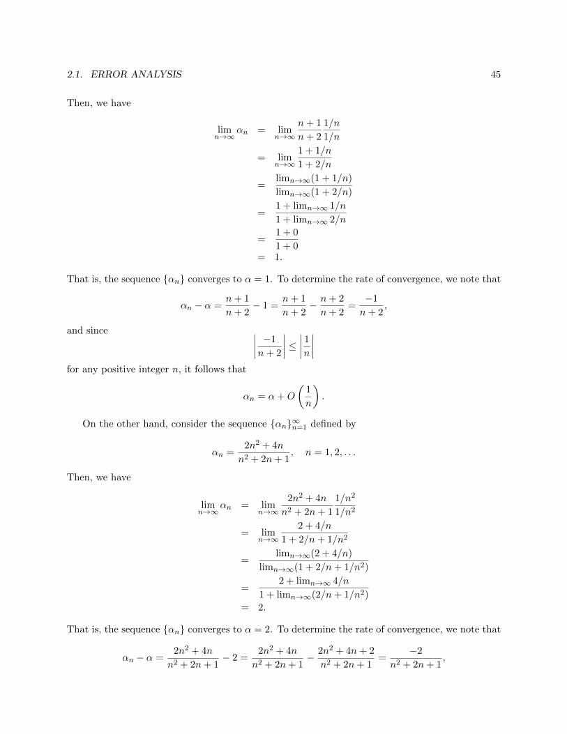
2.1. ERROR ANALYSIS 45
Then, we have
limn→∞
αn = limn→∞
n+ 1
n+ 2
1/n
1/n
= limn→∞
1 + 1/n
1 + 2/n
=limn→∞(1 + 1/n)
limn→∞(1 + 2/n)
=1 + limn→∞ 1/n
1 + limn→∞ 2/n
=1 + 0
1 + 0= 1.
That is, the sequence αn converges to α = 1. To determine the rate of convergence, we note that
αn − α =n+ 1
n+ 2− 1 =
n+ 1
n+ 2− n+ 2
n+ 2=−1
n+ 2,
and since ∣∣∣∣ −1
n+ 2
∣∣∣∣ ≤ ∣∣∣∣ 1n∣∣∣∣
for any positive integer n, it follows that
αn = α+O
(1
n
).
On the other hand, consider the sequence αn∞n=1 defined by
αn =2n2 + 4n
n2 + 2n+ 1, n = 1, 2, . . .
Then, we have
limn→∞
αn = limn→∞
2n2 + 4n
n2 + 2n+ 1
1/n2
1/n2
= limn→∞
2 + 4/n
1 + 2/n+ 1/n2
=limn→∞(2 + 4/n)
limn→∞(1 + 2/n+ 1/n2)
=2 + limn→∞ 4/n
1 + limn→∞(2/n+ 1/n2)
= 2.
That is, the sequence αn converges to α = 2. To determine the rate of convergence, we note that
αn − α =2n2 + 4n
n2 + 2n+ 1− 2 =
2n2 + 4n
n2 + 2n+ 1− 2n2 + 4n+ 2
n2 + 2n+ 1=
−2
n2 + 2n+ 1,
46 CHAPTER 2. APPROXIMATION IN NUMERICAL ANALYSIS
and since ∣∣∣∣ −2
n2 + 2n+ 1
∣∣∣∣ =
∣∣∣∣ 2
(n+ 1)2
∣∣∣∣ ≤ ∣∣∣∣ 2
n2
∣∣∣∣for any positive integer n, it follows that
αn = α+O
(1
n2
).
2
It is worth noting that Big-O notation is also useful for describing the runtime complexityof an algorithm in terms of the size of its input. In this context, we are not examining a convergentsequence, but rather describing the efficiency of an algorithm in a concise way.
Example 2.1.13 The number of arithmetic operations required to perform multiplication of twon× n real matrices, in the most straightforward manner, is f(n) = 2n3 − n2. For n ≥ 1, we have
|2n3 − n2| ≤ |2n3|+ |n2| ≤ |2n3|+ |n3| ≤ 3n3.
We conclude that f(n) is O(n3). 2
We can also use big-O notation to describe the rate of convergence of a function to a limit.
Example 2.1.14 Consider the function f(h) = 1 + 2h. Since this function is continuous for all h,we have
limh→0
f(h) = f(0) = 1.
It follows thatf(h)− f0 = (1 + 2h)− 1 = 2h = O(h),
so we can conclude that as h→ 0, 1 + 2h converges to 1 of order O(h). 2
Example 2.1.15 Consider the function f(h) = 1 + 4h+ 2h2. Since this function is continuous forall h, we have
limh→0
f(h) = f(0) = 1.
It follows thatf(h)− f0 = (1 + 4h+ 2h2)− 1 = 4h+ 2h2.
To determine the rate of convergence as h→ 0, we consider h in the interval [−1, 1]. In this interval,|h2| ≤ |h|. It follows that
|4h+ 2h2| ≤ |4h|+ |2h2|≤ |4h|+ |2h|≤ 6|h|.
Since there exists a constant C (namely, 6) such that |4h+ 2h2| ≤ C|h| for h satisfying |h| ≤ h0 forsome h0 (namely, 1), we can conclude that as h→ 0, 1 + 4h+ 2h2 converges to 1 of order O(h). 2
2.1. ERROR ANALYSIS 47
In general, when f(h) denotes an approximation that depends on h, and
f0 = limh→0
f(h)
denotes the exact value, f(h)− f0 represents the absolute error in the approximation f(h). Whenthis error is a polynomial in h, as in this example and the previous example, the rate of convergenceis O(hk) where k is the smallest exponent of h in the error. This is because as h → 0, thesmallest power of h approaches zero more slowly than higher powers, thereby making the dominantcontribution to the error.
By contrast, when determining the rate of convergence of a sequence αn as n → ∞, thehighest power of n determines the rate of convergence. As powers of n are negative if convergenceoccurs at all as n→∞, and powers of h are positive if convergence occurs at all as h→ 0, it can besaid that for either types of convergence, it is the exponent that is closest to zero that determinesthe rate of convergence.
Example 2.1.16 Consider the function f(h) = cosh. Since this function is continuous for all h,we have
limh→0
f(h) = f(0) = 1.
Using Taylor’s Theorem (Theorem A.6.1 in Section A.6), with center h0 = 0, we obtain
f(h) = f(0) + f ′(0)h+f ′′(ξ(h))
2h2,
where ξ(h) is between 0 and h. Substituting f(h) = cosh into the above, we obtain
cosh = 1− (sin 0)h+− cos ξ(h)
2h2,
or
cosh = 1− cos ξ(h)
2h2.
Because | cosx| ≤ 1 for all x, we have
| cosh− 1| =∣∣∣∣−cos ξ(h)
2h2
∣∣∣∣ ≤ 1
2h2,
so we can conclude that as h→ 0, cosh converges to 1 of order O(h2). 2
Exploration 2.1.12 Determine the rate of convergence of
limh→0
eh − h− 1
2h2 = 1.
Example 2.1.17 We will study the convergence of the centered difference approximation to thesecond derivative,
f ′′(x0) ≈ f(x0 + h)− 2f(x0) + f(x0 − h)
h2.
48 CHAPTER 2. APPROXIMATION IN NUMERICAL ANALYSIS
We assume that f ∈ C4[x0 − h, x0 + h]. That is, f belongs to the space of functions that have atleast four continuous derivatives on the interval [x0 − h, x0 + h].
Using Taylor’s Theorem (Theorem A.6.1), with n = 3 and center x0, we obtain the expansions
f(x0 + h) = f(x0) + f ′(x0)h+1
2f ′′(x0)h2 +
1
6f ′′′(x0)h3 +
1
24f (4)(ξ1)h4
f(x0 − h) = f(x0)− f ′(x0)h+1
2f ′′(x0)h2 − 1
6f ′′′(x0)h3 +
1
24f (4)(ξ2)h4
that each consist of a third-degree Taylor polynomial in h, and a remainder term that is O(h4).The remainders include the fourth derivative of f(x) evaluated at unknown points ξ1 ∈ [x0, x0 + h]and ξ2 ∈ [x0 − h, x0].
Adding these expansions yields
f(x0 + h) + f(x0 − h) = 2f(x0) + f ′′(x0)h2 +1
24h4[f (4)(ξ1) + f (4)(ξ2)].
After some algebraic manipulations, we obtain
f(x0 + h)− 2f(x0) + f(x0 − h)
h2= f ′′(x0) +
1
12h2 1
2[f (4)(ξ1) + f (4)(ξ2)].
Because f (4) is continuous on [x0 − h, x0 + h], we can apply the Intermediate Value Theorem(Theorem A.1.10 in Section A.1.5) to conclude that in the interval [ξ1, ξ2], there exists a point ξsuch that f (4)(ξ) is equal to the average of f (4)(ξ1) and f (4)(ξ2), which must lie between these twovalues.
We therefore have
f(x0 + h)− 2f(x0) + f(x0 − h)
h2= f ′′(x0) +
1
12h2f (4)(ξ)
and thus we have obtained the approximation
f ′′(x0) =f(x0 + h)− 2f(x0) + f(x0 − h)
h2− 1
12h2f (4)(ξ).
We conclude that the error is O(h2) because∣∣∣∣− 1
12h2f (4)(ξ)
∣∣∣∣ <=1
12Mh2
where |f (4)(x)| ≤M on [x0 − h, x0 + h]. 2
Try using the approach from the preceding example with other formulas for approximatingderivatives.
Exploration 2.1.13 Use Taylor’s Theorem to derive the error terms in the formulas
f ′(x0) ≈ f(x0 + h)− f(x0)
h, error = −h
2f ′′(ξ)
and
f ′(x0) ≈ f(x0 + h)− f(x0 − h)
2h, error = −h
2
6f ′′′(ξ).

2.2. COMPUTER ARITHMETIC 49
Exploration 2.1.14 Use both of the formulas from Exploration 2.1.13 to compute ap-proximations of f ′(x0), with f(x) = sinx, x0 = 1, and h = 10−1, 10−2, 10−3, and thenh = 10−14. What should the result be? What happens, and can you explain why?
If you can’t explain what happens for the smallest value of h, fortunately this will be addressed inSection 2.2.
2.1.6 Concept Check
1. For each of the following questions, answer true or false, with reasons:
(a) A more accurate algorithm for solving an ill-conditioned problem will make the problembetter conditioned.
(b) The choice of algorithm for solving a given problem does not affect the propagation oferror.
(c) A stable algorithm applied to a well-conditioned problem will produce an accurate so-lution.
2. What does it mean for a problem to be well-posed?
3. What are the two categories of error in numerical computation?
4. Explain the difference between truncation error and roundoff error.
5. When should error be measured using absolute error or relative error?
6. What does it mean for a problem to be well-conditioned?
7. Explain the distinction between a well-conditioned problem and a stable algorithm.
8. Explain the distinction between forward error and backward error.
9. How is backward error useful?
10. What does it mean to say that a sequence an is O(bn)?
11. What is the significance of the rate of convergence?
12. Explain the difference between how the rate of convergence is determined for a sequence anas n→∞ and a function f(h) as h→ 0.
13. What is the role that Taylor expansion plays in determining the rate of convergence?
2.2 Computer Arithmetic
In this section, we will focus on one type of error that occurs in all computation, whether performedby hand or on a computer: roundoff error. This error is due to the fact that in computation, realnumbers can only be represented using a finite number of digits. In general, it is not possible torepresent real numbers exactly with this limitation, and therefore they must be approximated byreal numbers that can be represented using a fixed number of digits, which is called the precision.
50 CHAPTER 2. APPROXIMATION IN NUMERICAL ANALYSIS
Exploration 2.2.1 Use scientific notation to write down approximations of 100π and10e consisting of five significant digits. Now multiply these approximations, retainingonly the same number of significant digits, and express the result in the same scientificnotation. How accurate is this approximation of 1000eπ? What is the percentage error?
As Exploration 2.2.1 illustrates, arithmetic operations applied to numbers that can be repre-sented exactly using a given precision do not necessarily produce a result that can be representedusing the same precision. It follows that if a fixed precision is used, then every arithmetic operationintroduces error into a computation.
Given that scientific computations can have several sources of error, one would think that itwould be foolish to compound the problem by performing arithmetic using fixed precision. However,using a fixed precision is actually far more practical than other options, and, as long as computationsare performed carefully, sufficient accuracy can still be achieved.
2.2.1 Floating-Point Representation
We now describe a typical system for representing real numbers on a computer.
Definition 2.2.1 (Floating-point Number System) Given integers β > 1, p ≥ 1,L, and U ≥ L, a floating-point number system F is defined to be the set of all realnumbers of the form
x = ±mβE .
The number m is the mantissa of x, and has the form
m =
p−1∑j=0
djβ−j
,
where each digit dj, j = 0, . . . , p− 1 is an integer satisfying 0 ≤ di ≤ β − 1. The numberE is called the exponent or the characteristic of x, and it is an integer satisfyingL ≤ E ≤ U . The integer p is called the precision of F, and β is called the base of F.
The term “floating-point” comes from the fact that as a number x ∈ F is multiplied by or divided bya power of β, the mantissa does not change, only the exponent. As a result, the decimal point shifts,or “floats,” to account for the changing exponent. Nearly all computers use a binary floating-pointsystem, in which β = 2.
Example 2.2.2 Let x = −117. Then, in a floating-point number system with base β = 10, x isrepresented as
x = −(1.17)102,
where 1.17 is the mantissa and 2 is the exponent. If the base β = 2, then we have
x = −(1.110101)26,
where 1.110101 is the mantissa and 6 is the exponent. The mantissa should be interpreted as a

2.2. COMPUTER ARITHMETIC 51
string of binary digits, rather than decimal digits; that is,
1.110101 = 1 · 20 + 1 · 2−1 + 1 · 2−2 + 0 · 2−3 + 1 · 2−4 + 0 · 2−5 + 1 · 2−6
= 1 +1
2+
1
4+
1
16+
1
64
=117
64
=117
26.
2
We now examine how to represent real numbers in a floating-point number system. For sim-plicity, we first consider the case of a decimal system, in which β = 10. Then, the floating-pointrepresentation of a number is essentially scientific notation, in which the significant digits of anumber are written separately from its magnitude.
Example 2.2.3 We write x = −1234.56789 as x = −1.23456789× 10³, so the exponent is E = 3,and the mantissa is m = 1.23456789. To represent this number exactly in a floating-point numbersystem with β = 10, we need at least nine digits in the mantissa; that is, we must have p ≥ 9. 2
For now, we will assume that the mantissa m has the property that the leading digit, d0, mustbe nonzero. This ensures that each number represented by a floating-point number system has aunique representation. This choice will be discussed in greater detail later in this section, when weintroduce normalized and denormalized floating-point numbers.
What is the largest possible mantissa in a system with β = 10 and p = 5? What if β = 2and p = 10? Express this value as both a sequence of binary digits, and as a decimal.
Show that if d0 6= 0, the mantissa m of a floating-point number must satisfy 1 ≤ m < β,where β is the base of the floating-point number system in question. Based on thepreceding exploration, can you provide a formula for the largest mantissa?
Assume that d0 6= 0. What is the exponent for the following numbers in the givenfloating-point number systems? Hint: Use the result of the preceding exploration.
1. x = 234597.34, β = 10
2. x = 0.00000178, β = 10
3. x = 998, β = 2
4. x = 0.01, β = 2
Show that if d0 6= 0, then the exponent E of a floating-point number x is given byE = blogβ |x|c, where β is the base of the floating-point number system, and bxc is thegreatest integer that is less than or equal to x (bxc is known as the greatest integer functionor the floor function; it is implemented by the floor function in Matlab). Hint: workwith the representation x = ±mβE .

52 CHAPTER 2. APPROXIMATION IN NUMERICAL ANALYSIS
Example 2.2.4 Consider the base of the natural logarithm, e, rounded to five significant digits:e ≈ 2.7183. To represent this number in a binary floating-point number system (that is, β = 2),we first obtain the exponent. Taking log2 2.7183 and rounding down, we obtain E = b1.4427c = 1.That is, 2.7183 = m× 21, where m = 2.7183/2 = 1.35915 is the mantissa.
To obtain a binary representation of the mantissa, we first take d0 = 1; by requiring d0 6= 0, ina binary system we must have d0 = 1 because that is the only remaining option. Subtracting off1, we focus on representing 0.35915 using binary digits. We repeat the following process: multiplyby 2, take the digit to the left of the decimal point, and subtract. The result of this process is:
1. 2× 0.35915 = 0.7183 =⇒ d1 = 0
2. 2× 0.7183 = 1.4366 =⇒ d2 = 1, then subtract 1
3. 2× 0.4366 = 0.8732 =⇒ d3 = 0
4. 2× 0.8732 = 1.7464 =⇒ d4 = 1, then subtract 1
5. 2× 0.7464 = 1.4928 =⇒ d5 = 1, then subtract 1
6. 2× 0.4928 = 0.9856 =⇒ d6 = 0
7. 2× 0.9856 = 1.9712 =⇒ d7 = 1, then subtract 1
8. 2× 0.9712 = 1.9424 =⇒ d8 = 1, then subtract 1
9. 2× 0.9424 = 1.8848 =⇒ d9 = 1, then subtract 1
10. 2× 0.8848 = 1.7696 =⇒ d10 = 1, then subtract 1
11. 2× 0.7696 = 1.5392 =⇒ d11 = 1, then subtract 1
12. 2× 0.5392 = 1.0784 =⇒ d12 = 1, then subtract 1
13. 2× 0.0784 = 0.1568 =⇒ d13 = 0
14. 2× 0.1568 = 0.3136 =⇒ d14 = 0
15. 2× 0.3136 = 0.6272 =⇒ d15 = 0
16. 2× 0.6272 = 1.2544 =⇒ d16 = 1, then subtract 1
17. 2× 0.2544 = 0.5088 =⇒ d17 = 0
18. 2× 0.5088 = 1.0176 =⇒ d18 = 1, then subtract 1
19. 2× 0.0176 = 0.0352 =⇒ d19 = 0
Limiting our floating-point number system to a precision of p = 20 digits, our mantissa is, in binary,1.0101101111110001010, which, in decimal, is equal to
m = 1 +1
22+
1
24+
1
25+
1
27+
1
28+
1
29+
1
210+
1
211+
1
212+
1
216+
1
218
= 1.359149932861328.
2.2. COMPUTER ARITHMETIC 53
It follows that our floating-point representation of 2.7183 is 2×1.359149932861328 = 2.718299865722656.We see that even with 20 binary digits of precision, we cannot represent 2.7183 exactly. Our floating-point number has a relative error of −4.9 × 10⁻⁸, which has a magnitude comparable to that of2−24. 2
Exploration 2.2.2 Using the approach from Example 2.2.4, express x = π as accuratelyas possible in a floating-point number system with base β = 2 and precision p = 12.
Exploration 2.2.3 Let β = 10. What are the smallest values of p and U , and the largestvalue of L, such that the numbers 239487.234 and 0.0000000034394 can be representedexactly in a floating-point number system of base β with precision p and exponent range[L,U ]?
2.2.1.1 Overflow and Underflow
A floating-point system F can only represent a finite subset of the real numbers. As such, it isimportant to know how large in magnitude a number can be and still be represented, at leastapproximately, by a number in F. Similarly, it is important to know how small in magnitude anumber can be and still be represented by a nonzero number in F; if its magnitude is too small,then it is most accurately represented by zero.
Exploration 2.2.4 Consider a floating-point number system with β = 10, p = 5,L = −20 and U = 20. What are the largest and smallest positive numbers that canbe represented in this system? How would you describe these values for a general floating-point number system with β = 10?
The answer to Exploration 2.2.4 leads to the following formal definition, that applies to any validbase.
Definition 2.2.5 (Underflow, Overflow) Let F be a floating-point number system.The smallest positive number in F is called the underflow level, and it has the value
UFL = mmin βL,
where L is the smallest valid exponent and mmin is the smallest mantissa. The largestpositive number in F is called the overflow level, and it has the value
OFL = βU+1(1− β−p).
The value of mmin depends on whether floating-point numbers are normalized in F; this pointwill be discussed later. The overflow level is the value obtained by setting each digit in the mantissato β − 1 and using the largest possible value, U , for the exponent.
Exploration 2.2.5 Determine the value of OFL for a floating-point system with baseβ = 2, precision p = 53, and largest exponent U = 1023.
It is important to note that the real numbers that can be represented in F are not equally spacedalong the real line. Numbers having the same exponent are equally spaced, and the spacing betweennumbers in F decreases as their magnitude decreases.
54 CHAPTER 2. APPROXIMATION IN NUMERICAL ANALYSIS
2.2.1.2 Normalization
It is common to normalize floating-point numbers by specifying that the leading digit d0 of themantissa be nonzero. In a binary system, with β = 2, this implies that the leading digit is equalto 1, and therefore need not be stored. In addition to the benefit of gaining one additional bit ofprecision, normalization also ensures that each floating-point number has a unique representation.
Example 2.2.6 Without normalization, the number 3.14 could also be represented as 0.314× 101
or 0.00314×10³, but with normalization, these two alternative representations would not be allowed,because in both cases the leading digit of the mantissa is zero. 2
Exploration 2.2.6 Consider a floating-point number system with β = 10, p = 5, L =−20 and U = 20. Write down three representations of the closest representable numberto 100π.
Exploration 2.2.7 How does the answer to Exploration 2.2.4 change if numbers arenormalized?
One drawback of normalization is that fewer numbers near zero can be represented exactly thanif normalization is not used. One workaround is a practice called gradual underflow, in which theleading digit of the mantissa is allowed to be zero when the exponent is equal to L, thus allowingsmaller values of the mantissa. In such a system, the number UFL is equal to βL−p+1, whereas ina normalized system, UFL = βL.
Exploration 2.2.8 Determine the value of UFL for a floating-point system with baseβ = 2, precision p = 53, and smallest exponent L = −1022, both with and withoutnormalization.
2.2.1.3 Rounding
A number that can be represented exactly in a floating-point system is called a machine number.Since only finitely many real numbers are machine numbers, it is necessary to determine how non-machine numbers are to be approximated by machine numbers. The process of choosing a machinenumber to approximate a non-machine number is called rounding, and the error introduced bysuch an approximation is called roundoff error. Given a real number x, the machine numberobtained by rounding x is denoted by fl(x).
In most floating-point systems, rounding is achieved by one of two strategies:
• chopping, or rounding to zero, is the simplest strategy, in which the base-β expansion ofa number is truncated after the first p digits. As a result, fl(x) is the unique machine numberbetween 0 and x that is nearest to x.
• rounding to nearest sets fl(x) to be the machine number that is closest to x in absolutevalue; if two numbers satisfy this property, then an appropriate tie-breaking rule must beused, such as setting fl(x) equal to the choice whose last digit is even.
Example 2.2.7 Suppose we are using a floating-point system with β = 10 (decimal), with p = 4significant digits. Then, if we use chopping, or rounding to zero, we have fl(2/3) = 0.6666, whereasif we use rounding to nearest, then we have fl(2/3) = 0.6667. 2
2.2. COMPUTER ARITHMETIC 55
Example 2.2.8 When rounding to even in decimal, 88.5 is rounded to 88, not 89, so that thelast digit is even, while 89.5 is rounded to 90, again to make the last digit even. 2
2.2.1.4 Machine Precision
In error analysis, it is necessary to estimate error incurred in each step of a computation. As such,it is desirable to know an upper bound for the relative error introduced by rounding. This leads tothe following definition.
Definition 2.2.9 (Machine Precision) Let F be a floating-point number system. Theunit roundoff or machine precision, denoted by u, is the real number that satisfies∣∣∣∣fl(x)− x
x
∣∣∣∣ ≤ u
for any real number x such that UFL < x < OFL.
An intuitive definition of u is that it is the smallest positive number such that
fl (1 + u) > 1.
The value of u depends on the rounding strategy that is used. If rounding toward zero is used,then u = β1−p, whereas if rounding to nearest is used, u = 1
2β1−p.
It is important to avoid confusing u with the underflow level UFL. The unit roundoff is deter-mined by the number of digits in the mantissa, whereas the underflow level is determined by therange of allowed exponents. However, we do have the relation that 0 < UFL < u.
n analysis of roundoff error, it is assumed that fl(x op y) = (x op y)(1 + δ), where op is anarithmetic operation and δ is an unknown constant satisfying |δ| ≤ u. From this assumption, itcan be seen that the relative error in fl(x op y) is |δ|. In the case of addition, the relative backwarderror in each operand is also |δ|.
2.2.1.5 The IEEE Floating-Point Standard
In fact, most computers conform to the IEEE standard for floating-point arithmetic. The stan-dard specifies, among other things, how floating-point numbers are to be represented in memory.Two representations are given, one for single-precision and one for double-precision.
Under the standard, single-precision floating-point numbers occupy 4 bytes in memory, with23 bits used for the mantissa, 8 for the exponent, and one for the sign. IEEE double-precisionfloating-point numbers occupy eight bytes in memory, with 52 bits used for the mantissa, 11 forthe exponent, and one for the sign. That is, in the IEEE floating-point standard, p = 24 for singleprecision, and p = 53 for double precision, even though only 23 and 52 bits, respectively, are usedto store mantissas.
Example 2.2.10 The following table summarizes the main aspects of a general floating-pointsystem and a double-precision floating-point system that uses a 52-bit mantissa and 11-bit exponent.For both systems, we assume that rounding to nearest is used, and that normalization is used. 2

56 CHAPTER 2. APPROXIMATION IN NUMERICAL ANALYSIS
General Double Precision
Form of machine number ±mβE ±1.d1d2 · · · d522E
Precision p 53
Exponent range L ≤ E ≤ U −1023 ≤ E ≤ 1024
UFL (Underflow Level) βL 2−1023
OFL (Overflow Level) βU+1(1− β−p) 21025(1− 2−53)
u 12β
1−p 2−53
Exploration 2.2.9 Are the values for UFL and OFL given in the table above the actualvalues used in the IEEE double-precision floating point system? Experiment with powersof 2 in Matlab to find out. What are the largest and smallest positive numbers you canrepresent? Can you explain any discrepancies between these values and the ones in thetable?
One can gain insight into the representation of IEEE double-precision floating-point numbersusing format hex in Matlab. Consider the following output:
>> format hex
>> 4075/64
ans =
404fd60000000000
>> format long
>> ans
ans =
63.671875000000000
The hexadecimal, or base 16, representation of the number 4075/64 = 63.671875 can readily beconverted to binary, because 16 = 24 and therefore each hexadecimal digit corresponds to fourbinary digits.
For convenience, we use the following conversion table,
Decimal Hexadecimal Binary Decimal Hexadecimal Binary
0 0 0000 8 8 10001 1 0001 9 9 10012 2 0010 10 a 10103 3 0011 11 b 10114 4 0100 12 c 11005 5 0101 13 d 11016 6 0110 14 e 11107 7 0111 15 f 1111
where each binary number should be interpreted in the same way as a number in decimal is naturallyinterpreted, only with base 2 instead of base 10. That is, the rightmost digit is multiplied by 20 = 1,and then added to the next digit to the left times 21 = 2, plus the next digit to the left times 22 = 4,and so on. For example,
13 = 1101 = 1× 23 + 1× 22 + 0× 21 + 1× 20 = 8 + 4 + 0 + 1.
Using this table, the binary representation of 404fd60000000000 is
2.2. COMPUTER ARITHMETIC 57
0100 0000 0100 1111 1101 0110 0000 0000 0000 0000 0000 0000 0000 0000 0000 0000
where spaces are introduced to separate sequences of binary digits corresponding to the originalhexadecimal digits.
Now, we interpret this sequence of 64 binary digits, or bits, in terms of the IEEE double-precision floating-point standard. Reading from left to right, the first bit, 0, is the sign bit, whichindicates that the number is positive; a sign bit of 1 is used for a negative number. The next 11bits, 10000000100, represents the unsigned integer 210 + 22 = 1028. We subtract 1023 from thisvalue to obtain the exponent E = 5.
Finally, the twelve leading binary digits of the mantissa are 111111010110, followed by fortydigits that are zero. Because the number is normalized, there is an implied leading digit d0 = 1. Thebits of the mantissa that are explicitly stored correspond to the digits d1, d2, . . . , dp−1 in Definition2.2.1, with p = 53. It follows that the value represented by the mantissa is
52∑j=0
dj2−j = 1 +
1
2+
1
4+
1
8+
1
16+
1
32+
1
64+
1
256+
1
1024+
1
2048=
4075
2048.
Therefore, the number represented is
(−1)0 × 25 × 4075
2048=
4075
64,
where the three numbers multiplied on the left side account for the sign bit 0, the exponent 5, andmantissa 4075/2048, respectively.
2.2.2 Issues with Floating-Point Arithmetic
We now discuss the various issues that arise when performing floating-point arithmetic, orfinite-precision arithmetic, which approximates arithmetic operations on real numbers.
2.2.2.1 Loss of Precision
When adding or subtracting floating-point numbers, it is necessary to shift one of the operandsso that both operands have the same exponent, before adding or subtracting the mantissas. As aresult, digits of precision are lost in the operand that is smaller in magnitude, and the result of theoperation cannot be represented using a machine number. In fact, if x is the smaller operand andy is the larger operand, and |x| < |y|u, then the result of the operation will simply be y (or −y, ify is to be subtracted from x), since the entire value of x is lost in rounding the result.
Example 2.2.11 Consider a floating-point system with β = 10, p = 10, L = −20 and U = 20. Ifx = 2× 10⁴ and y = 3× 10⁻¹⁰, then the exact value of x+ y is 20000.0000000003, but that cannotbe represented in this floating-point system because 15 digits are needed to represent this numberbut only p = 10 digits are available. The floating-point representation of the sum would simply bex, because |y| < |x|u, where u = 1
210−10 is the machine precision. 2

58 CHAPTER 2. APPROXIMATION IN NUMERICAL ANALYSIS
Exploration 2.2.10 Consider the evaluation of the summation
n∑i=1
xi,
where each term xi is positive. Will the sum be computed more accurately in floating-point arithmetic if the numbers are added in order from smallest to largest, or largest tosmallest? Justify your answer.
In multiplication or division, the operands need not be shifted, but the mantissas, when mul-tiplied or divided, cannot necessarily be represented using only p digits of precision. The productof two mantissas requires 2p digits to be represented exactly, while the quotient of two mantissascould conceivably require infinitely many digits.
2.2.2.2 Violation of Arithmetic Rules
Because floating-point arithmetic operations are not exact, they do not follow all of the laws of realarithmetic. In particular, while floating-point arithmetic is still commutative, it is not associative;i.e., x+ (y + z) 6= (x+ y) + z in floating-point arithmetic.
Exploration 2.2.11 In Matlab, generate three random numbers x, y and z, and com-pute x + (y + z) and (x + y) + z. Do they agree? Try this a few times with differentrandom numbers, of different magnitudes, and observe what happens. What would haveto be true of x, y and z to cause a significant deviation?
2.2.2.3 Overflow and Underflow
Furthermore, overflow or underflow may occur depending on the exponents of the operands, sincetheir sum or difference may lie outside of the interval [L,U ].
Example 2.2.12 Consider a floating-point system with β = 10, L = −20 and U = 20. Then thenumbers x = 4×10¹⁸ and y = −2×10⁻¹⁷ can be represented exactly in this system, but computingx/y = −2 × 1035 would cause overflow because the exponent of 35 is greater than U . Similarly,computing y2 = 4×10⁻³⁴ would cause underflow, because the exponent of −34 is less than L. Thisvalue would therefore be rounded to zero. 2
Exploration 2.2.12 Consider the formula z =√x2 + y2. Explain how overflow can
occur in computing z, even if x, y and z all have magnitudes that can be represented.How can this formula be rewritten so that overflow does not occur?
Exploration 2.2.13 Let x ∈ Rn. Use the result of Exploration 2.2.12 to describe analgorithm for computing
‖x‖2 =
(n∑i=1
x2i
)1/2
in such a way as to prevent overflow.
2.2. COMPUTER ARITHMETIC 59
2.2.2.4 Cancellation
Subtraction of floating-point numbers presents a unique difficulty, in addition to the rounding errorpreviously discussed.
Exploration 2.2.14 When performing the subtraction
0.345769258233−0.345769258174
how many significant digits are included in the result? In general, if the two numbersbeing subtracted have p significant digits, and the first (most significant, or left to right)m digits agree, how many significant digits, at most, can the result have?
In an extreme case, if the two operands differ by less than u, then the result contains no correctdigits; it consists entirely of roundoff error from previous computations. This phenomenon is knownas catastrophic cancellation, or cancellation error. Because of the highly detrimental effectof this cancellation, it is important to ensure that no steps in a computation compute small valuesfrom relatively large operands. Often, computations can be rearranged to avoid this risky practice.
Example 2.2.13 Consider the quadratic equation
ax2 + bx+ c = 0,
which has the solutions
x1 =−b+
√b2 − 4ac
2a, x2 =
−b−√b2 − 4ac
2a.
Suppose that b > 0. Then, in computing x1, we encounter catastrophic cancellation if b is muchlarger than a and c, because this implies that
√b2 − 4ac ≈ b and as a result we are subtracting
two numbers that are nearly equal in computing the numerator. On the other hand, if b < 0, weencounter this same difficulty in computing x2.
Suppose that we use 4-digit rounding arithmetic to compute the roots of the equation
x2 + 10, 000x+ 1 = 0.
Then, we obtain x1 = 0 and x2 = −10, 000. Clearly, x1 is incorrect because if we substitute x = 0into the equation then we obtain the contradiction 1 = 0. In fact, if we use 7-digit roundingarithmetic then we obtain the same result. Only if we use at least 8 digits of precision do we obtainroots that are reasonably correct,
x1 ≈ −1× 10⁻⁴, x2 ≈ −9.9999999× 10³.
2
Exploration 2.2.15 Use an algebraic manipulation commonly used on expressions in-volving square roots to obtain a new quadratic formula that circumvents the cancellationerror exhibited in Example 2.2.13. Try this formula on the same quadratic equation, with4-digit rounding arithmetic.

60 CHAPTER 2. APPROXIMATION IN NUMERICAL ANALYSIS
As the following explorations illustrate, cancellation error can occur in a variety of situations,so it is a phenomenon that one should always be aware of when designing numerical algorithms.
Exploration 2.2.16 Use the Matlab function randn to generate 1000 normally dis-tributed random numbers with mean 1000 and standard deviation 0.1. Then, use theseformulas to compute the variance:
1. 1n
∑ni=1(xi − x)2
2.(
1n
∑ni=1 x
2i
)− x2
where x is the mean. How do the results differ? Which formula is more susceptible toissues with floating-point arithmetic, and why?
Exploration 2.2.17 Recall Exploration 2.1.14, in which two approximations of thederivative were tested using various values of the spacing h. In light of the discussionin this section, explain the behavior for the case of h = 10−14.
Exploration 2.2.18 Consider the expression
1
1− x− 1
1 + x.
For which values of x can the evaluation of this expression, as written, have an issue dueto floating-point arithmetic? Rewrite the expression to address the issue.
Exploration 2.2.19 Assume that x ≈ y, and that |x|, |y| 1. Consider the equation
x2 − y2 = (x− y)(x+ y).
Which side of this expression is evaluated more accurately with floating-point arithmetic?
2.2.3 Concept Check
1. For each of the following questions, answer true or false, with reasons:
(a) Floating-point numbers are uniformly distributed.
(b) If two real numbers can be represented exactly in a floating-point number system, thenthe result of an arithmetic operation on these numbers can also be represented exactly.
(c) Floating-point addition is commutative.
(d) Floating-point addition is associative.
(e) IEEE double-precision floating-point numbers have a mantissa that is twice the lengthof IEEE single-precision floating-point numbers.
(f) The unit roundoff, or machine precision, is the smallest positive number that can beadded to one and produce a result greater than one in the floating-point number system.
2. Describe the four numbers (β, p, L, U) that define a floating-point number system.
2.3. ADDITIONAL RESOURCES 61
3. Define underflow and overflow. Which one is more problematic, and why?
4. Of the four basic arithmetic operations (addition, subtraction, multiplication and division),which ones can not produce overflow when applied to two positive numbers?
5. What is the benefit of normalizing floating-point numbers? What is a good reason not tonormalize them? Explain how the use of gradual underflow yields a “best-of-both-worlds”situation.
6. Explain the difference between chopping and rounding. What is the benefit of rounding toeven?
7. What is cancellation error, and under what circumstances does it arise?
8. Give an example of a number that can be represented exactly in decimal, but not in binary.
9. Explain the distinction between the unit roundoff u and the underflow level UFL.
2.3 Additional Resources
The concept of backward error analysis was introduced by James Wilkinson in the context ofnumerical linear algebra; see for example [198, 199]. An early treatment of the notion of conditioningcan be found in [157]. “Big-O” notation, and variations thereof, are covered extensively by Graham,Knuth and Patashnik [82]. In this chapter, this notation was used primarily to discuss convergence,but in later chapters we will also use it to discuss the complexity, or, informally, “running time”of algorithms, as in Example 2.1.13. Complexity theory, as applied to algorithms in general, ispresented in [23].
Wilkinson was also a pioneer in the area of roundoff error analysis; see [199]. The IEEE floating-point standard is published in [99]; a tutorial is also provided in [78]. The web page of WilliamKahan, who was a leading figure in the development of the standard, is an excellent resourcefor information about floating-point arithmetic: http://people.eecs.berkeley.edu/~wkahan/.Overton’s textbook on the subject [142] is an accessible treatment that includes discussion offloating-point architecture, programming language support, and the concepts of conditioning, sta-bility and cancellation. Higham’s text [95] provides a thorough error analysis of roundoff error andstability of numerical algorithms, along with historical perspective.
Books that focus on the hardware aspects of computer arithmetic are [112, 139, 145]. Beyond thescope of this book is interval arithmetic [4, 102, 133], in which arithmetic operations are performednot on numbers but intervals that account for measurement and rounding errors.
2.4 Exercises
1. Let f(x) = x − y, where y is a fixed constant. Use the relative condition number of f(x) toexplain why subtraction suffers from cancellation error.
2. Let x, y > 0 be such that x ≈ y. It follows that ln(x) − ln(y) is susceptible to cancellationerror. Use the relative condition number to explain why the equivalent expression ln(x/y)is also problematic, even though it does not involve subtraction. Hint: treat ln(x/y) as afunction of x with constant y, as in Exercise 1.
62 CHAPTER 2. APPROXIMATION IN NUMERICAL ANALYSIS
3. In Matlab, form a vector of n + 1 equally spaced points x0, x1, x2, . . . , xn on [0, 1], withspacing h = 1/n, in two different ways:
(a) x0 = 0, xi = xi−1 + h, i = 1, 2, . . . , n
(b) xi = ih, i = 0, 1, 2, . . . , n
Which approach is more accurate, and why?
4. Find the IEEE double-precision floating-point representation of 0.1. How would the represen-tation change if chopping was used instead of rounding? Hint: Use format hex in Matlabto display this value in hexadecimal.
5. Use Example 2.2.13 to write a Matlab function [x1,x2]=quadroots(a,b,c) to computethe roots x1 and x2 of the quadratic equation ax2 + bx + c = 0 in such a way as to avoidcancellation error.
6. Graph the function f(x) = (x − 1)6 on the interval [0.995, 1.005], using at least 100 equallyspaced points, in two different ways: a) by evaluating (x − 1)6, exactly as written, for eachx-value, and b) by expanding (x−1)6. Use one of the functions in Section 1.2.17 to help withthis. Explain the discrepancy in the graphs.
7. Consider a floating-point number system with β = 2 in which all numbers are normalized.Describe the circumstances in which u < UFL. Your answer should be a relationship betweenp and L. How does your answer change if unnormalized numbers are used? In both cases,assume rounding is used rather than chopping.
8. Write a Matlab function [s,m,e]=dissectfp(x) that accepts as input a double-precisionfloating-point number x and returns as output the components of the floating-point represen-tation of x: the sign s, the mantissa m and the exponent e. s is 1 if x is positive; otherwiseit is −1. The mantissa x consists of the binary digits d0, d1, . . . , dp−1, from Definition 2.2.1,where p = 53, that form a double-precision floating-point number x0 where 0 ≤ x0 < 2.The exponent e must be an integer in the interval [−1022, 1023]. Make sure to account fordenormalized numbers.
9. The Matlab function round, when used with a second input argument n, can be used toround a number x (specified as the first input) to n digits, whether they are the n mostsignificant digits, or the first n digits to the right of the decimal point. Write functionsroundsig and rounddec that perform rounding in these manners. Compare your results tothose returned by round with the appropriate usage. Consult the help page for round asneeded.
10. As a follow-up to Exploration 2.2.10, consider the following algorithm, due to W. Kahan [105]and called compensated summation, for computing the sum of n numbers x1, x2, . . . , xn:
s = x1
c = 0for i = 2, . . . , n do
y = xi − c

2.4. EXERCISES 63
t = s+ yc = (t− s)− ys = t
end for
Explain why this is a more efficient approach to computing the sum than the most accurateapproach found in Exploration 2.2.10.

64 CHAPTER 2. APPROXIMATION IN NUMERICAL ANALYSIS

Part III
Data Fitting and FunctionApproximation
65

Chapter 6
Polynomial Interpolation
Calculus provides many tools that can be used to understand the behavior of functions, but in mostcases it is necessary for these functions to be continuous or differentiable. This presents a problemin most “real” applications, in which functions are used to model relationships between quantities,but our only knowledge of these functions consists of a set of discrete data points, where the datais obtained from measurements. Therefore, we need to be able to construct continuous functionsbased on discrete data.
The problem of constructing such a continuous function is called data fitting. In this lecture,we discuss a special case of data fitting known as interpolation, in which the goal is to finda linear combination of n known functions to fit a set of data that imposes n constraints, thusguaranteeing a unique solution that fits the data exactly, rather than approximately. The broaderterm “constraints” is used, rather than simply “data points”, since the description of the data mayinclude additional information such as rates of change or requirements that the fitting functionhave a certain number of continuous derivatives.
When it comes to the study of functions using calculus, polynomials are particularly simple towork with. Therefore, in this course we will focus on the problem of constructing a polynomialthat, in some sense, fits given data. We first discuss some algorithms for computing the uniquepolynomial pn(x) of degree n that satisfies pn(xi) = yi, i = 0, . . . , n, where the points (xi, yi) aregiven. The points x0, x1, . . . , xn are called interpolation points. The polynomial pn(x) is calledthe interpolating polynomial of the data (x0, y0), (x1, y1), . . ., (xn, yn). At first, we will assumethat the interpolation points are all distinct; this assumption will be relaxed in a later section.
6.1 Existence and Uniqueness
Suppose that we express the interpolating polynomial pn(x) in the familiar power form
pn(x) = a0 + a1x+ a2x2 + · · ·+ anx
n. (6.1)
Then, a straightforward method of computing the interpolating polynomial is to solve the equationspn(xi) = yi, for i = 0, 1, . . . , n, for the unknown coefficients aj , j = 0, 1, . . . , n.
67

68 CHAPTER 6. POLYNOMIAL INTERPOLATION
Exploration 6.1.1 Solve the system of equations
a0 + a1x0 = y0,
a0 + a1x1 = y1
for the coefficients of the linear function p1(x) = a0 + a1x that interpolates the data(x0, y0), (x1, y1). What is the system of equations that must be solved to compute thecoefficients a0, a1 and a2 of the quadratic function p2(x) = a0+a1x+a2x
2 that interpolatesthe data (x0, y0), (x1, y1), (x2, y2)? Express both systems of equations in matrix-vectorform.
For general n, computing the coefficients a0, a1, . . . , an of pn(x) requires solving the system oflinear equations Vna = y, where the entries of Vn are defined by [Vn]ij = xji , i, j = 0, . . . , n, wherex0, x1, . . . , xn are the points at which the data y0, y1, . . . , yn are obtained. The basis 1, x, . . . , xnof the space of polynomials of degree n is called the monomial basis, and the correspondingmatrix Vn is called the Vandermonde matrix for the points x0, x1, . . . , xn. Because the x-valuesx0, x1, . . . , xn are distinct, Vn is invertible (see Exploration 6.1.2), which ensures that the systemVna = y has a unique solution.
Unfortunately, this approach to computing pn(x) is not practical. Solving this system of equa-tions requires O(n3) floating-point operations; we will see that O(n2) is possible. Furthermore, theVandermonde matrix can be ill-conditioned, especially when the interpolation points x0, x1, . . . , xnare close together.
Exploration 6.1.2 Write down the Vandermonde matrix Vn for the pointsx0, x1, . . . , xn. Show that
detVn =
n∏i=0
i−1∏j=0
(xi − xj).
Conclude that the system of equations Vna = y has a unique solution.
Exploration 6.1.3 In this exploration, we consider another approach to proving theuniqueness of the interpolating polynomial. Let pn(x) and qn(x) be polynomials of de-gree n such that pn(xi) = qn(xi) = yi for i = 0, 1, 2, . . . , n. Prove that pn(x) ≡ qn(x) forall x.
Exploration 6.1.4 Suppose we express the interpolating polynomial of degree one in theform
p1(x) = a0(x− x1) + a1(x− x0).
What is the matrix of the system of equations p1(xi) = yi, for i = 0, 1? How should theform of the interpolating polynomial of degree two, p2(x), be chosen to obtain an equallysimple system of equations to solve for the coefficients a0, a1, and a2?
6.1.1 Concept Check
1. What is data fitting and why is it necessary?
2. Why is it desirable to approximate functions using polynomials?
6.2. LAGRANGE INTERPOLATION 69
3. Explain why the polynomial of degree n that interpolates the data (x0, y0), (x1, y1), . . .,(xn, yn) is unique.
4. Why is it not practical to use a Vandermonde matrix to obtain an interpolating polynomial?
6.2 Lagrange Interpolation
As we have seen, expressing the interpolating polynomial pn(x) in power form (6.1) leads to animpractical approach to obtaining its coefficients. Therefore, we will construct pn(x) using a rep-resentation other than the monomial basis. That is, we will represent pn(x) as
pn(x) =n∑i=0
aiϕi(x),
for some choice of polynomials ϕ0(x), ϕ1(x), . . . , ϕn(x). This is equivalent to solving the linearsystem Pa = y, where the matrix P has entries pij = ϕj(xi). By choosing the basis functionsϕi(x)ni=0 judiciously, we can obtain a simpler system of linear equations to solve.
6.2.1 Lagrange Polynomials
In Lagrange interpolation, the matrix P is simply the identity matrix, by virtue of the fact thatthe interpolating polynomial is written in the form
pn(x) =n∑j=0
yjLn,j(x),
where the polynomials Ln,jnj=0 have the property that
Ln,j(xi) =
1 if i = j0 if i 6= j
.
The polynomials Ln,j, j = 0, . . . , n, are called the Lagrange polynomials for the interpolationpoints x0, x1, . . ., xn.
To obtain a formula for the Lagrange polynomials, we note that the above definition specifiesthe roots of Ln,j(x): xi, for i 6= j. It follows that Ln,j(x) has the form
Ln,j(x) = βj
n∏i=0,i 6=j
(x− xi)
for some constant βj . Substituting x = xj and requiring Ln,j(xj) = 1 yields βj =∏ni=0,i 6=j
1(xj−xi) .
We conclude that
Ln,j(x) =
n∏k=0,k 6=j
x− xkxj − xk
. (6.2)
As the following result indicates, the problem of polynomial interpolation can be solved usingLagrange polynomials.
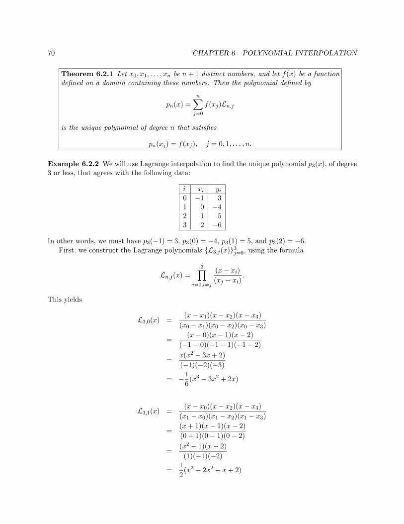
70 CHAPTER 6. POLYNOMIAL INTERPOLATION
Theorem 6.2.1 Let x0, x1, . . . , xn be n+ 1 distinct numbers, and let f(x) be a functiondefined on a domain containing these numbers. Then the polynomial defined by
pn(x) =n∑j=0
f(xj)Ln,j
is the unique polynomial of degree n that satisfies
pn(xj) = f(xj), j = 0, 1, . . . , n.
Example 6.2.2 We will use Lagrange interpolation to find the unique polynomial p3(x), of degree3 or less, that agrees with the following data:
i xi yi0 −1 31 0 −42 1 53 2 −6
In other words, we must have p3(−1) = 3, p3(0) = −4, p3(1) = 5, and p3(2) = −6.
First, we construct the Lagrange polynomials L3,j(x)3j=0, using the formula
Ln,j(x) =3∏
i=0,i 6=j
(x− xi)(xj − xi)
.
This yields
L3,0(x) =(x− x1)(x− x2)(x− x3)
(x0 − x1)(x0 − x2)(x0 − x3)
=(x− 0)(x− 1)(x− 2)
(−1− 0)(−1− 1)(−1− 2)
=x(x2 − 3x+ 2)
(−1)(−2)(−3)
= −1
6(x3 − 3x2 + 2x)
L3,1(x) =(x− x0)(x− x2)(x− x3)
(x1 − x0)(x1 − x2)(x1 − x3)
=(x+ 1)(x− 1)(x− 2)
(0 + 1)(0− 1)(0− 2)
=(x2 − 1)(x− 2)
(1)(−1)(−2)
=1
2(x3 − 2x2 − x+ 2)

6.2. LAGRANGE INTERPOLATION 71
L3,2(x) =(x− x0)(x− x1)(x− x3)
(x2 − x0)(x2 − x1)(x2 − x3)
=(x+ 1)(x− 0)(x− 2)
(1 + 1)(1− 0)(1− 2)
=x(x2 − x− 2)
(2)(1)(−1)
= −1
2(x3 − x2 − 2x)
L3,3(x) =(x− x0)(x− x1)(x− x2)
(x3 − x0)(x3 − x1)(x3 − x2)
=(x+ 1)(x− 0)(x− 1)
(2 + 1)(2− 0)(2− 1)
=x(x2 − 1)
(3)(2)(1)
=1
6(x3 − x).
By substituting xi for x in each Lagrange polynomial L3,j(x), for j = 0, 1, 2, 3, it can be verifiedthat
L3,j(xi) =
1 if i = j0 if i 6= j
.
It follows that the Lagrange interpolating polynomial p3(x) is given by
p3(x) =3∑j=0
yjL3,j(x)
= y0L3,0(x) + y1L3,1(x) + y2L3,2(x) + y3L3,3(x)
= (3)
(−1
6
)(x3 − 3x2 + 2x) + (−4)
1
2(x3 − 2x2 − x+ 2) + (5)
(−1
2
)(x3 − x2 − 2x) +
(−6)1
6(x3 − x)
= −1
2(x3 − 3x2 + 2x) + (−2)(x3 − 2x2 − x+ 2)− 5
2(x3 − x2 − 2x)− (x3 − x)
=
(−1
2− 2− 5
2− 1
)x3 +
(3
2+ 4 +
5
2
)x2 + (−1 + 2 + 5 + 1)x− 4
= −6x3 + 8x2 + 7x− 4.
Substituting each xi, for i = 0, 1, 2, 3, into p3(x), we can verify that we obtain p3(xi) = yi in eachcase. 2
The Matlab function p=polyfit(x,y,n) performs polynomial interpolation. The input ar-guments x and y are vectors consisting of the x- and y-coordinates of the data points to be fit.The input argument n is the degree of the interpolating polynomial; for Lagrange interpolation, itshould be set equal to one less than the length of x. The output p is a row vector of coefficients
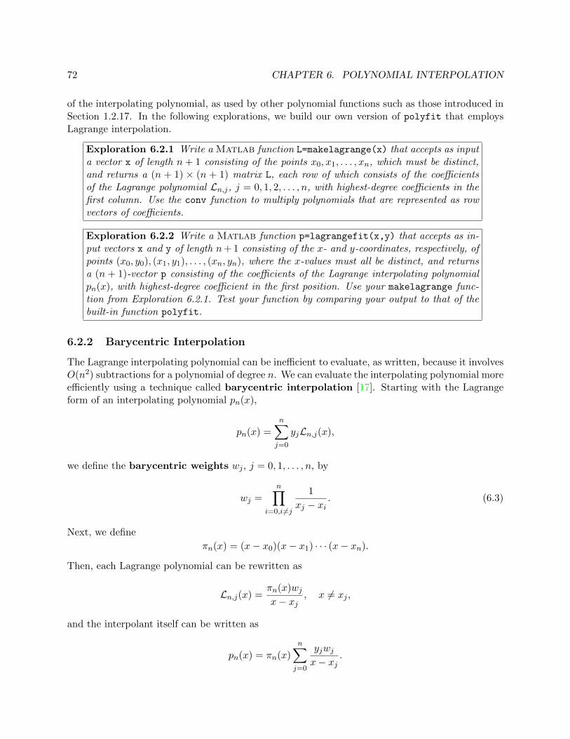
72 CHAPTER 6. POLYNOMIAL INTERPOLATION
of the interpolating polynomial, as used by other polynomial functions such as those introduced inSection 1.2.17. In the following explorations, we build our own version of polyfit that employsLagrange interpolation.
Exploration 6.2.1 Write a Matlab function L=makelagrange(x) that accepts as inputa vector x of length n + 1 consisting of the points x0, x1, . . . , xn, which must be distinct,and returns a (n + 1) × (n + 1) matrix L, each row of which consists of the coefficientsof the Lagrange polynomial Ln,j, j = 0, 1, 2, . . . , n, with highest-degree coefficients in thefirst column. Use the conv function to multiply polynomials that are represented as rowvectors of coefficients.
Exploration 6.2.2 Write a Matlab function p=lagrangefit(x,y) that accepts as in-put vectors x and y of length n+ 1 consisting of the x- and y-coordinates, respectively, ofpoints (x0, y0), (x1, y1), . . . , (xn, yn), where the x-values must all be distinct, and returnsa (n + 1)-vector p consisting of the coefficients of the Lagrange interpolating polynomialpn(x), with highest-degree coefficient in the first position. Use your makelagrange func-tion from Exploration 6.2.1. Test your function by comparing your output to that of thebuilt-in function polyfit.
6.2.2 Barycentric Interpolation
The Lagrange interpolating polynomial can be inefficient to evaluate, as written, because it involvesO(n2) subtractions for a polynomial of degree n. We can evaluate the interpolating polynomial moreefficiently using a technique called barycentric interpolation [17]. Starting with the Lagrangeform of an interpolating polynomial pn(x),
pn(x) =n∑j=0
yjLn,j(x),
we define the barycentric weights wj , j = 0, 1, . . . , n, by
wj =n∏
i=0,i 6=j
1
xj − xi. (6.3)
Next, we define
πn(x) = (x− x0)(x− x1) · · · (x− xn).
Then, each Lagrange polynomial can be rewritten as
Ln,j(x) =πn(x)wjx− xj
, x 6= xj ,
and the interpolant itself can be written as
pn(x) = πn(x)n∑j=0
yjwjx− xj
.
6.3. DIVIDED DIFFERENCES 73
However, if we let yj = 1 for j = 0, 1, . . . , n, we have
1 = πn(x)
n∑j=0
wjx− xj
.
Dividing the previous two equations yields
pn(x) =
n∑j=0
yjwjx− xj
n∑j=0
wjx− xj
. (6.4)
Although O(n2) products are needed to compute the barycentric weights, they need only be com-puted once, and then re-used for each x, which is not the case with the Lagrange form.
Exploration 6.2.3 Write a Matlab function w=baryweights(x) that accepts as inputa vector x of length n + 1, consisting of the distinct interpolation points x0, x1, . . . , xn,and returns a vector w of length n+ 1 consisting of the barycentric weights wj as definedin (6.3).
Exploration 6.2.4 Write a Matlab function yy=lagrangeval(x,y,xx) that ac-cepts as input vectors x and y, both of length n + 1, representing the data points(x0, y0), (x1, y1), . . . , (xn, yn), and a vector of x-values xx. This function uses the barycen-tric weights (6.3), as computed by the function baryweights from Exploration 6.2.3, tocompute the value of the Lagrange interpolating polynomial for the given data points ateach x-value in xx using (6.4). The corresponding y-values must be returned in the vectoryy, which must have the same dimensions as xx.
6.2.3 Concept Check
1. What properties characterize Lagrange polynomials?
2. What is the advantage of using Lagrange polynomials to express the interpolating polynomial,compared to using a Vandermonde matrix?
3. What is a drawback of using Lagrange polynomials?
4. What is the benefit of using barycentric interpolation?
6.3 Divided Differences
While the Lagrange polynomials are easy to compute, they are difficult to work with. Furthermore,if new interpolation points are added, all of the Lagrange polynomials must be recomputed. Unfor-tunately, it is not uncommon, in practice, to add to an existing set of interpolation points. It maybe determined after computing the kth-degree interpolating polynomial pk(x) of a function f(x)
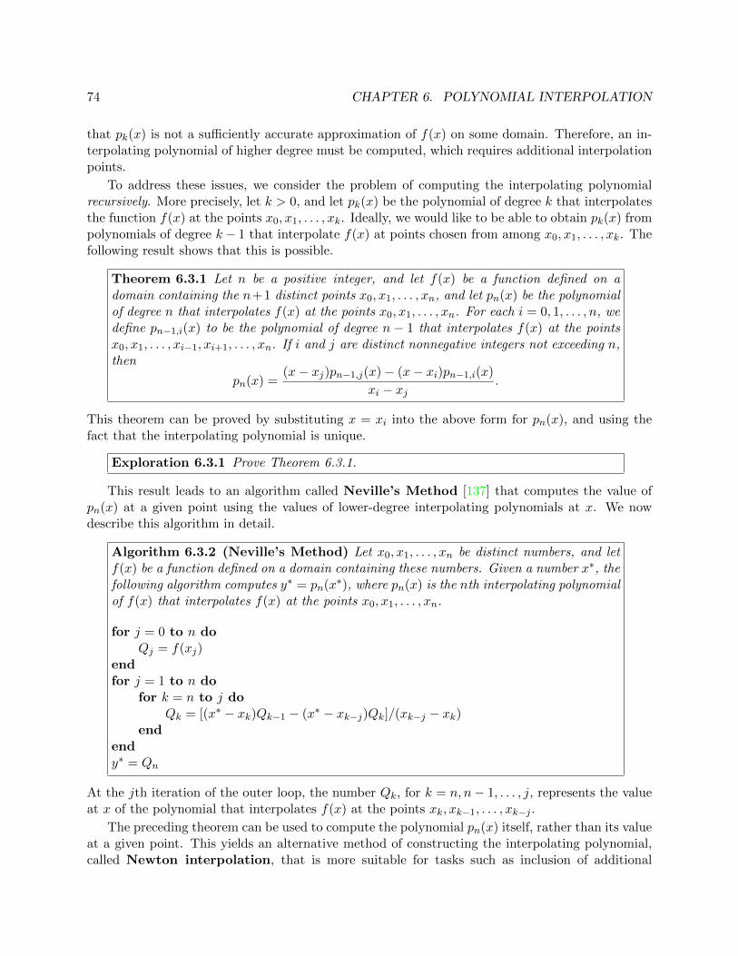
74 CHAPTER 6. POLYNOMIAL INTERPOLATION
that pk(x) is not a sufficiently accurate approximation of f(x) on some domain. Therefore, an in-terpolating polynomial of higher degree must be computed, which requires additional interpolationpoints.
To address these issues, we consider the problem of computing the interpolating polynomialrecursively. More precisely, let k > 0, and let pk(x) be the polynomial of degree k that interpolatesthe function f(x) at the points x0, x1, . . . , xk. Ideally, we would like to be able to obtain pk(x) frompolynomials of degree k− 1 that interpolate f(x) at points chosen from among x0, x1, . . . , xk. Thefollowing result shows that this is possible.
Theorem 6.3.1 Let n be a positive integer, and let f(x) be a function defined on adomain containing the n+1 distinct points x0, x1, . . . , xn, and let pn(x) be the polynomialof degree n that interpolates f(x) at the points x0, x1, . . . , xn. For each i = 0, 1, . . . , n, wedefine pn−1,i(x) to be the polynomial of degree n − 1 that interpolates f(x) at the pointsx0, x1, . . . , xi−1, xi+1, . . . , xn. If i and j are distinct nonnegative integers not exceeding n,then
pn(x) =(x− xj)pn−1,j(x)− (x− xi)pn−1,i(x)
xi − xj.
This theorem can be proved by substituting x = xi into the above form for pn(x), and using thefact that the interpolating polynomial is unique.
Exploration 6.3.1 Prove Theorem 6.3.1.
This result leads to an algorithm called Neville’s Method [137] that computes the value ofpn(x) at a given point using the values of lower-degree interpolating polynomials at x. We nowdescribe this algorithm in detail.
Algorithm 6.3.2 (Neville’s Method) Let x0, x1, . . . , xn be distinct numbers, and letf(x) be a function defined on a domain containing these numbers. Given a number x∗, thefollowing algorithm computes y∗ = pn(x∗), where pn(x) is the nth interpolating polynomialof f(x) that interpolates f(x) at the points x0, x1, . . . , xn.
for j = 0 to n doQj = f(xj)
endfor j = 1 to n do
for k = n to j doQk = [(x∗ − xk)Qk−1 − (x∗ − xk−j)Qk]/(xk−j − xk)
endendy∗ = Qn
At the jth iteration of the outer loop, the number Qk, for k = n, n− 1, . . . , j, represents the valueat x of the polynomial that interpolates f(x) at the points xk, xk−1, . . . , xk−j .
The preceding theorem can be used to compute the polynomial pn(x) itself, rather than its valueat a given point. This yields an alternative method of constructing the interpolating polynomial,called Newton interpolation, that is more suitable for tasks such as inclusion of additional
6.3. DIVIDED DIFFERENCES 75
interpolation points. The basic idea is to represent interpolating polynomials using the Newtonform, which uses linear factors involving the interpolation points, instead of monomials of the formxj .
6.3.1 Newton Form
Recall that if the interpolation points x0, . . . , xn are distinct, then the process of finding a polyno-mial that passes through the points (xi, yi), i = 0, . . . , n, is equivalent to solving a system of linearequations Ax = b that has a unique solution. The matrix A is determined by the choice of basis forthe space of polynomials of degree n or less. Each entry aij of A is the value of the jth polynomialin the basis at the point xi.
In Newton interpolation, the matrix A is upper triangular, and the basis functions are definedto be the set Nj(x)nj=0, where
N0(x) = 1, Nj(x) =
j−1∏k=0
(x− xk), j = 1, . . . , n.
The advantage of Newton interpolation is that the interpolating polynomial is easily updated asinterpolation points are added, since the basis functions Nj(x), j = 0, . . . , n, do not change fromthe addition of the new points.
Using Theorem 6.3.1, it can be shown that the coefficients cj of the Newton interpolatingpolynomial
pn(x) =n∑j=0
cjNj(x) (6.5)
are given by
cj = f [x0, . . . , xj ] (6.6)
where f [x0, . . . , xj ] denotes the divided difference of x0, . . . , xj . The divided difference is definedas follows:
f [xi] = yi, (6.7)
f [xi, xi+1] =yi+1 − yixi+1 − xi
, (6.8)
f [xi, xi+1, . . . , xi+k] =f [xi+1, . . . , xi+k]− f [xi, . . . , xi+k−1]
xi+k − xi. (6.9)
This definition implies that for each nonnegative integer j, the divided difference f [x0, x1, . . . , xj ]only depends on the interpolation points x0, x1, . . . , xj and the value of f(x) at these points. Itfollows that the addition of new interpolation points does not change the coefficients c0, . . . , cn.Specifically, we have
pn+1(x) = pn(x) +yn+1 − pn(xn+1)
Nn+1(xn+1)Nn+1(x).
This ease of updating makes Newton interpolation the most commonly used method of obtainingthe interpolating polynomial.
76 CHAPTER 6. POLYNOMIAL INTERPOLATION
Exploration 6.3.2 Use Theorem 6.3.1 and the definition of divided differences givenby (6.7)-(6.9) to prove, by induction, that the coefficients c0, c1, . . . , cn of pn(x) in theNewton form (6.5) are given by (6.6).
The following result shows how the Newton interpolating polynomial bears a resemblance to aTaylor polynomial.
Theorem 6.3.3 Let f be n times continuously differentiable on [a, b], and letx0, x1, . . . , xn be distinct points in [a, b]. Then there exists a number ξ ∈ [a, b] suchthat
f [x0, x1, . . . , xn] =f (n)(ξ)
n!.
We now discover how Theorem 6.3.3 can be proved. First, we examine the simplest cases.
Exploration 6.3.3 Prove Theorem 6.3.3 for the cases of n = 1 and n = 2, using thedefinition of divided differences, the Mean Value Theorem (Theorem A.5.3), and Taylor’sTheorem (Theorem A.6.1).
The approach used in Exploration 6.3.3 is difficult to generalize to larger values of n, so we nowconsider a different approach.
Exploration 6.3.4 Let pn(x) be the interpolating polynomial for f(x) at pointsx0, x1, . . . , xn ∈ [a, b], and assume that f is n times differentiable. Use Rolle’s Theo-
rem (Theorem A.5.1) to prove that p(n)n (ξ) = f (n)(ξ) for some point ξ ∈ [a, b].
Exploration 6.3.5 Use Exploration 6.3.4 to prove Theorem 6.3.3. Hint: Express pn(x)as the sum of pn−1(x) and an additional term, where pn−1(x) interpolates f(x) at any nof the points x0, x1, . . . , xn.
6.3.2 Computing the Newton Interpolating Polynomial
We now describe in detail how to compute the coefficients cj = f [x0, x1, . . . , xj ] of the Newtoninterpolating polynomial pn(x), and how to evaluate pn(x) efficiently using these coefficients.
The computation of the coefficients proceeds by filling in the entries of a divided-differencetable. This is a triangular table consisting of n+ 1 columns, where n is the degree of the interpo-lating polynomial to be computed. For j = 0, 1, . . . , n, the jth column contains n− j entries, whichare the divided differences f [xk, xk+1, . . . , xk+j ], for k = 0, 1, . . . , n − j. Here we show a divideddifference table for n = 3:
i xi f [xi] f [xi, xi+1] f [xi, . . . , xi+2] f [xi, . . . , xi+3]
0 x0 f(x0)f [x0, x1]
1 x1 f(x1) f [x0, x1, x2]f [x1, x2] f [x0, x1, x2, x3]
2 x2 f(x2) f [x1, x2, x3]f [x2, x3]
3 x3 f(x3)
6.3. DIVIDED DIFFERENCES 77
We construct this table by filling in the n+ 1 entries in column 0, which are the trivial divideddifferences f [xj ] = f(xj), for j = 0, 1, . . . , n. Then, we use the recursive definition of the divideddifferences to fill in the entries of subsequent columns. Once the construction of the table iscomplete, we can obtain the coefficients of the Newton interpolating polynomial from the firstentry in each column, which is f [x0, x1, . . . , xj ], for j = 0, 1, . . . , n.
Algorithm 6.3.4 (Divided-Difference Table) Given n + 1 distinct interpolationpoints x0, x1, . . . , xn, and the values of a function f(x) at these points, the followingalgorithm computes the coefficients cj = f [x0, x1, . . . , xj ] of the Newton interpolatingpolynomial. The following algorithm computes these coefficients.
for i = 0, 1, . . . , n dodi,0 = f(xi)
endfor j = 1, 2, . . . , n do
for i = n, n− 1, . . . , j dodi,j = (di,j−1 − di−1,j−1)/(xi − xi−j)
endendfor j = 0, 1, . . . , n do
cj = dj,jend
In a practical implementation of this algorithm, we do not need to store the entire table, becausewe only need the first entry in each column. Because each column has one fewer entry than theprevious column, we can overwrite all of the other entries that we do not need. Algorithm 6.3.4does not implement this idea, but it can be modified to do so.
Modify Algorithm 6.3.4 so that it uses at most O(n) storage; that is, it does not need tostore a matrix di,jni,j=0 of divided differences.
Example 6.3.5 We will use Newton interpolation to construct the third-degree polynomial p3(x)that fits the data
i xi f(xi)
0 −1 31 0 −42 1 53 2 −6
In other words, we must have p3(−1) = 3, p3(0) = −4, p3(1) = 5, and p3(2) = −6.
First, we construct the divided-difference table from this data. The divided differences in thetable are computed as follows:
f [x0] = f(x0) = 3, f [x1] = f(x1) = −4, f [x2] = f(x2) = 5, f [x3] = f(x3) = −6,
78 CHAPTER 6. POLYNOMIAL INTERPOLATION
f [x0, x1] =f [x1]− f [x0]
x1 − x0=−4− 3
0− (−1)= −7
f [x1, x2] =f [x2]− f [x1]
x2 − x1=
5− (−4)
1− 0= 9
f [x2, x3] =f [x3]− f [x2]
x3 − x2=−6− 5
2− 1= −11
f [x0, x1, x2] =f [x1, x2]− f [x0, x1]
x2 − x0
=9− (−7)
1− (−1)
= 8
f [x1, x2, x3] =f [x2, x3]− f [x1, x2]
x3 − x1
=−11− 9
2− 0= −10
f [x0, x1, x2, x3] =f [x1, x2, x3]− f [x0, x1, x2]
x3 − x0
=−10− 8
2− (−1)
= −6
The resulting divided-difference table is
x0 = −1 f [x0] = 3f [x0, x1] = −7
x1 = 0 f [x1] = −4 f [x0, x1, x2] = 8f [x1, x2] = 9 f [x0, x1, x2, x3] = −6
x2 = 1 f [x2] = 5 f [x1, x2, x3] = −10f [x2, x3] = −11
x3 = 2 f [x3] = −6
It follows that the interpolating polynomial p3(x) can be expressed in Newton form as follows:
p3(x) =3∑j=0
f [x0, . . . , xj ]
j−1∏i=0
(x− xi)
= f [x0] + f [x0, x1](x− x0) + f [x0, x1, x2](x− x0)(x− x1) +
f [x0, x1, x2, x3](x− x0)(x− x1)(x− x2)
= 3− 7(x+ 1) + 8(x+ 1)x− 6(x+ 1)x(x− 1).
We see that Newton interpolation produces an interpolating polynomial that is in the Newton form,with centers x0 = −1, x1 = 0, and x2 = 1. 2

6.3. DIVIDED DIFFERENCES 79
Exploration 6.3.6 Write a Matlab function c=divdiffs(x,y) that computes the di-vided difference table from the given data stored in the input vectors x and y, and returnsa vector c consisting of the divided differences f [x0, . . . , xj ], j = 0, 1, 2, . . . , n, where n+1is the length of both x and y.
Once the coefficients have been computed, we can use nested multiplication to evaluate theresulting interpolating polynomial, which is represented using the Newton form
pn(x) =n∑j=0
cjNj(x)
=
n∑j=0
f [x0, x1, . . . , xj ]
j−1∏i=0
(x− xi)
= f [x0] + f [x0, x1](x− x0) + f [x0, x1, x2](x− x0)(x− x1) +
f [x0, x1, . . . , xn](x− x0)(x− x1) · · · (x− xn−1). (6.10)
Algorithm 6.3.6 (Nested Multiplication) Given n + 1 distinct interpolation pointsx0, x1, . . . , xn and the coefficients cj = f [x0, x1, . . . , xj ], j = 0, 1, . . . , n, of the Newtoninterpolating polynomial pn(x), the following algorithm computes y = pn(x) for a givenreal number x.
bn = cnfor i = n− 1, n− 2, . . . , 0 do
bi = ci + (x− xi)bi+1
endy = b0
Exploration 6.3.7 Write a Matlab function yy=newtonval(x,y,xx) that acceptsas input vectors x and y, both of length n + 1, representing the data points(x0, y0), (x1, y1), . . . , (xn, yn), and a vector of x-values xx. This function uses Algorithm6.3.6, as well as the function divdiffs from Exploration 6.3.6, to compute the valueof the Newton interpolating polynomial for the given data points at each x-value in xx.The corresponding y-values must be returned in the vector yy, which must have the samedimensions as xx.
Nested multiplication has another useful application: the conversion of a polynomial fromNewton form to power form
pn(x) = a0 + a1x+ a2x2 + · · ·+ anx
n.
This is illustrated in the following example.
Example 6.3.7 Consider the interpolating polynomial obtained in the previous example,
p3(x) = 3− 7(x+ 1) + 8(x+ 1)x− 6(x+ 1)x(x− 1).

80 CHAPTER 6. POLYNOMIAL INTERPOLATION
We will use nested multiplication to write this polynomial in power form
p3(x) = b3x3 + b2x
2 + b1x+ b0.
This requires repeatedly applying nested multiplication to a polynomial of the form
p(x) = c0 + c1(x− x0) + c2(x− x0)(x− x1) + c3(x− x0)(x− x1)(x− x2),
and for each application it will perform the following steps,
b3 = c3
b2 = c2 + (z − x2)b3
b1 = c1 + (z − x1)b2
b0 = c0 + (z − x0)b1,
where, in this example, we will set z = 0 each time.
The numbers b0, b1, b2 and b3 computed by the algorithm are the coefficients of p(x) in theNewton form, with the centers x0, x1 and x2 changed to z, x0 and x1; that is,
p(x) = b0 + b1(x− z) + b2(x− z)(x− x0) + b3(x− z)(x− x0)(x− x1).
It follows that b0 = p(z), which is why this algorithm is the preferred method for evaluating apolynomial in Newton form at a given point z.
It should be noted that the algorithm can be derived by writing p(x) in the nested form
p(x) = c0 + (x− x0)[c1 + (x− x1)[c2 + (x− x2)c3]]
and computing p(z) as follows:
p(z) = c0 + (z − x0)[c1 + (z − x1)[c2 + (z − x2)c3]]
= c0 + (z − x0)[c1 + (z − x1)[c2 + (z − x2)b3]]
= c0 + (z − x0)[c1 + (z − x1)b2]
= c0 + (z − x0)b1
= b0.
Initially, we have
p(x) = 3− 7(x+ 1) + 8(x+ 1)x− 6(x+ 1)x(x− 1),
so the coefficients of p(x) in this Newton form are
c0 = 3, c1 = −7, c2 = 8, c3 = −6,
with the centers
x0 = −1, x1 = 0, x2 = 1.
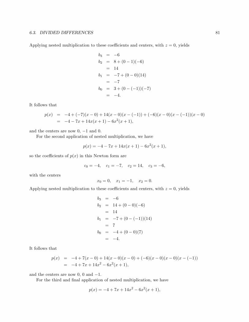
6.3. DIVIDED DIFFERENCES 81
Applying nested multiplication to these coefficients and centers, with z = 0, yields
b3 = −6
b2 = 8 + (0− 1)(−6)
= 14
b1 = −7 + (0− 0)(14)
= −7
b0 = 3 + (0− (−1))(−7)
= −4.
It follows that
p(x) = −4 + (−7)(x− 0) + 14(x− 0)(x− (−1)) + (−6)(x− 0)(x− (−1))(x− 0)
= −4− 7x+ 14x(x+ 1)− 6x2(x+ 1),
and the centers are now 0, −1 and 0.For the second application of nested multiplication, we have
p(x) = −4− 7x+ 14x(x+ 1)− 6x2(x+ 1),
so the coefficients of p(x) in this Newton form are
c0 = −4, c1 = −7, c2 = 14, c3 = −6,
with the centersx0 = 0, x1 = −1, x2 = 0.
Applying nested multiplication to these coefficients and centers, with z = 0, yields
b3 = −6
b2 = 14 + (0− 0)(−6)
= 14
b1 = −7 + (0− (−1))(14)
= 7
b0 = −4 + (0− 0)(7)
= −4.
It follows that
p(x) = −4 + 7(x− 0) + 14(x− 0)(x− 0) + (−6)(x− 0)(x− 0)(x− (−1))
= −4 + 7x+ 14x2 − 6x2(x+ 1),
and the centers are now 0, 0 and −1.For the third and final application of nested multiplication, we have
p(x) = −4 + 7x+ 14x2 − 6x2(x+ 1),
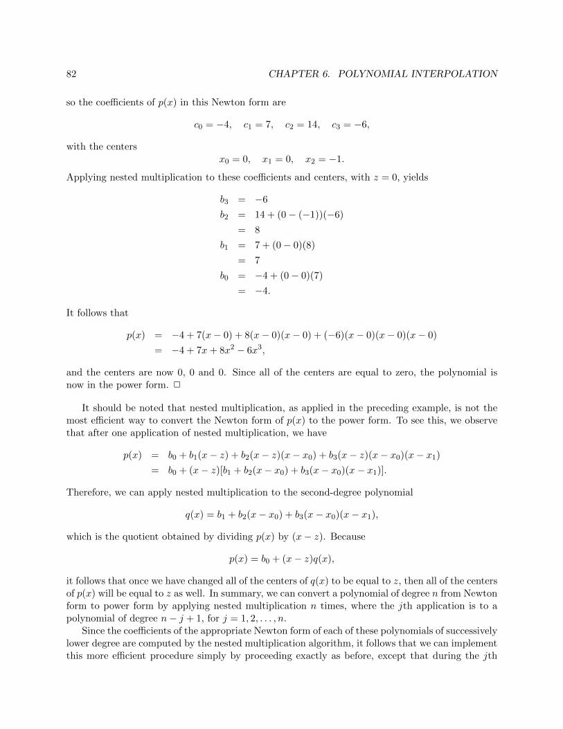
82 CHAPTER 6. POLYNOMIAL INTERPOLATION
so the coefficients of p(x) in this Newton form are
c0 = −4, c1 = 7, c2 = 14, c3 = −6,
with the centersx0 = 0, x1 = 0, x2 = −1.
Applying nested multiplication to these coefficients and centers, with z = 0, yields
b3 = −6
b2 = 14 + (0− (−1))(−6)
= 8
b1 = 7 + (0− 0)(8)
= 7
b0 = −4 + (0− 0)(7)
= −4.
It follows that
p(x) = −4 + 7(x− 0) + 8(x− 0)(x− 0) + (−6)(x− 0)(x− 0)(x− 0)
= −4 + 7x+ 8x2 − 6x3,
and the centers are now 0, 0 and 0. Since all of the centers are equal to zero, the polynomial isnow in the power form. 2
It should be noted that nested multiplication, as applied in the preceding example, is not themost efficient way to convert the Newton form of p(x) to the power form. To see this, we observethat after one application of nested multiplication, we have
p(x) = b0 + b1(x− z) + b2(x− z)(x− x0) + b3(x− z)(x− x0)(x− x1)
= b0 + (x− z)[b1 + b2(x− x0) + b3(x− x0)(x− x1)].
Therefore, we can apply nested multiplication to the second-degree polynomial
q(x) = b1 + b2(x− x0) + b3(x− x0)(x− x1),
which is the quotient obtained by dividing p(x) by (x− z). Because
p(x) = b0 + (x− z)q(x),
it follows that once we have changed all of the centers of q(x) to be equal to z, then all of the centersof p(x) will be equal to z as well. In summary, we can convert a polynomial of degree n from Newtonform to power form by applying nested multiplication n times, where the jth application is to apolynomial of degree n− j + 1, for j = 1, 2, . . . , n.
Since the coefficients of the appropriate Newton form of each of these polynomials of successivelylower degree are computed by the nested multiplication algorithm, it follows that we can implementthis more efficient procedure simply by proceeding exactly as before, except that during the jth
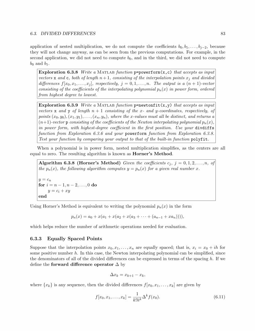
6.3. DIVIDED DIFFERENCES 83
application of nested multiplication, we do not compute the coefficients b0, b1, . . . , bj−2, becausethey will not change anyway, as can be seen from the previous computations. For example, in thesecond application, we did not need to compute b0, and in the third, we did not need to computeb0 and b1.
Exploration 6.3.8 Write a Matlab function p=powerform(x,c) that accepts as inputvectors x and c, both of length n+ 1, consisting of the interpolation points xj and divideddifferences f [x0, x1, . . . , xj ], respectively, j = 0, 1, . . . , n. The output is a (n + 1)-vectorconsisting of the coefficients of the interpolating polynomial pn(x) in power form, orderedfrom highest degree to lowest.
Exploration 6.3.9 Write a Matlab function p=newtonfit(x,y) that accepts as inputvectors x and y of length n + 1 consisting of the x- and y-coordinates, respectively, ofpoints (x0, y0), (x1, y1), . . . , (xn, yn), where the x-values must all be distinct, and returns a(n+1)-vector p consisting of the coefficients of the Newton interpolating polynomial pn(x),in power form, with highest-degree coefficient in the first position. Use your divdiffs
function from Exploration 6.3.6 and your powerform function from Exploration 6.3.8.Test your function by comparing your output to that of the built-in function polyfit.
When a polynomial is in power form, nested multiplication simplifies, as the centers are allequal to zero. The resulting algorithm is known as Horner’s Method.
Algorithm 6.3.8 (Horner’s Method) Given the coefficients cj, j = 0, 1, 2, . . . , n, ofthe pn(x), the following algorithm computes y = pn(x) for a given real number x.
y = cnfor i = n− 1, n− 2, . . . , 0 do
y = ci + xyend
Using Horner’s Method is equivalent to writing the polynomial pn(x) in the form
pn(x) = a0 + x(a1 + x(a2 + x(a3 + · · ·+ (an−1 + xan)))),
which helps reduce the number of arithmetic operations needed for evaluation.
6.3.3 Equally Spaced Points
Suppose that the interpolation points x0, x1, . . . , xn are equally spaced; that is, xi = x0 + ih forsome positive number h. In this case, the Newton interpolating polynomial can be simplified, sincethe denominators of all of the divided differences can be expressed in terms of the spacing h. If wedefine the forward difference operator ∆ by
∆xk = xk+1 − xk,
where xk is any sequence, then the divided differences f [x0, x1, . . . , xk] are given by
f [x0, x1, . . . , xk] =1
k!hk∆kf(x0). (6.11)
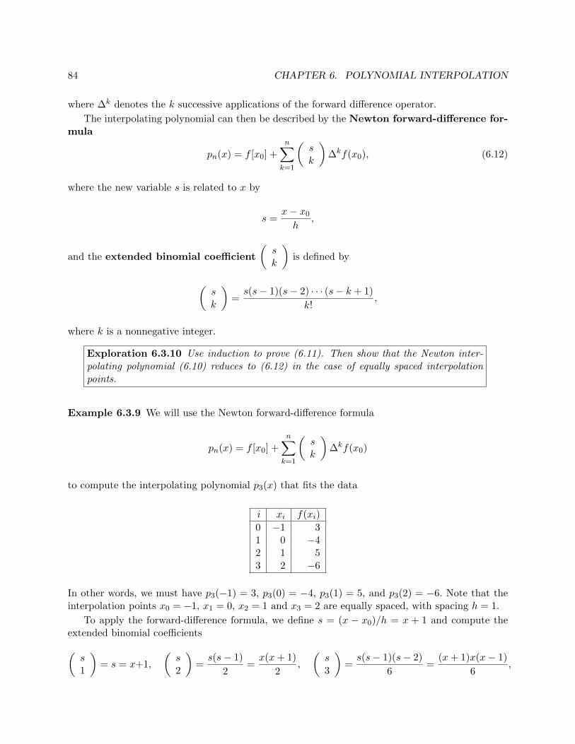
84 CHAPTER 6. POLYNOMIAL INTERPOLATION
where ∆k denotes the k successive applications of the forward difference operator.
The interpolating polynomial can then be described by the Newton forward-difference for-mula
pn(x) = f [x0] +n∑k=1
(sk
)∆kf(x0), (6.12)
where the new variable s is related to x by
s =x− x0
h,
and the extended binomial coefficient
(sk
)is defined by
(sk
)=s(s− 1)(s− 2) · · · (s− k + 1)
k!,
where k is a nonnegative integer.
Exploration 6.3.10 Use induction to prove (6.11). Then show that the Newton inter-polating polynomial (6.10) reduces to (6.12) in the case of equally spaced interpolationpoints.
Example 6.3.9 We will use the Newton forward-difference formula
pn(x) = f [x0] +n∑k=1
(sk
)∆kf(x0)
to compute the interpolating polynomial p3(x) that fits the data
i xi f(xi)
0 −1 31 0 −42 1 53 2 −6
In other words, we must have p3(−1) = 3, p3(0) = −4, p3(1) = 5, and p3(2) = −6. Note that theinterpolation points x0 = −1, x1 = 0, x2 = 1 and x3 = 2 are equally spaced, with spacing h = 1.
To apply the forward-difference formula, we define s = (x − x0)/h = x + 1 and compute theextended binomial coefficients(s1
)= s = x+1,
(s2
)=s(s− 1)
2=x(x+ 1)
2,
(s3
)=s(s− 1)(s− 2)
6=
(x+ 1)x(x− 1)
6,
6.3. DIVIDED DIFFERENCES 85
and then the coefficients
f [x0] = f(x0) = 3,
∆f(x0) = f(x1)− f(x0) = −7,
∆2f(x0) = ∆(∆f(x0))
= ∆[f(x1)− f(x0)]
= [f(x2)− f(x1)]− [f(x1)− f(x0)]
= f(x2)− 2f(x1) + f(x0) = 16
∆3f(x0) = ∆(∆2f(x0))
= ∆[f(x2)− 2f(x1) + f(x0)]
= [f(x3)− f(x2)]− 2[f(x2)− f(x1)] + [f(x1)− f(x0)]
= f(x3)− 3f(x2) + 3f(x1)− f(x0) = −36.
It follows that
p3(x) = f [x0] +
3∑k=1
(sk
)∆kf(x0)
= 3 +
(s1
)∆f(x0) +
(s1
)∆2f(x0) +
(s2
)∆3f(x0)
= 3 + (x+ 1)(−7) +x(x+ 1)
216 +
(x+ 1)x(x− 1)
6(−36)
= 3− 7(x+ 1) + 8(x+ 1)x− 6(x+ 1)x(x− 1).
Note that the forward-difference formula computes the same form of the interpolating polynomialas the Newton divided-difference formula. 2
Exploration 6.3.11 Define the backward difference operator ∇ by
∇xk = xk − xk−1,
for any sequence xk. Then derive the Newton backward-difference formula
pn(x) = f [xn] +n∑k=1
(−1)k(−sk
)∇kf(xn),
where s = (x − xn)/h, and the preceding definition of the extended binomial coefficientapplies.
Exploration 6.3.12 Look up the documentation for the Matlab function diff. Thenwrite functions yy=newtonforwdiff(x,y,xx) and yy=newtonbackdiff(x,y,xx) thatuse diff to implement the Newton forward-difference and Newton backward-differenceformulas, respectively, and evaluate the interpolating polynomial pn(x), where n =length(x)− 1, at the elements of xx. The resulting values must be returned in yy.

86 CHAPTER 6. POLYNOMIAL INTERPOLATION
6.3.4 Concept Check
1. What is Neville’s Method?
2. What advantage does Newton interpolation have over Lagrange interpolation?
3. What are divided differences, and what role do they play in Newton interpolation?
4. Describe the relationship between divided differences f [x0, x1, . . . , xk] and higher-order deriva-tives of f(x).
5. What is a divided difference table, and what role does it play in Newton interpolation?
6. Once the divided difference table is completed, how is the Newton interpolating polynomialobtained?
7. What is Horner’s method?
8. What is nested multiplication, and how does it relate to Horner’s method?
9. How can the interpolating polynomial be converted from Newton form to power form?
10. How does Newton interpolation simplify in the case of equally spaced points?
6.4 Error Analysis
In some applications, the interpolating polynomial pn(x) is used to fit a known function f(x)at the points x0, . . . , xn, usually because f(x) is not feasible for tasks such as differentiation orintegration that are easy for polynomials, or because it is not easy to evaluate f(x) at points otherthan the interpolation points. In such an application, it is desirable to determine how well pn(x)approximates f(x).
6.4.1 Error Estimation
From Theorem 6.3.3, we can obtain the following result.
Theorem 6.4.1 (Interpolation error) If f is n + 1 times continuously differentiableon [a, b], and pn(x) is the unique polynomial of degree n that interpolates f(x) at the n+1distinct points x0, x1, . . . , xn in [a, b], then for each x ∈ [a, b],
f(x)− pn(x) =f (n+1)(ξ(x))
(n+ 1)!
n∏j=0
(x− xj),
where ξ(x) ∈ [a, b].
It is interesting to note that the error closely resembles the Taylor remainder Rn(x).
Exploration 6.4.1 Prove Theorem 6.4.1. Hint: work with the Newton interpolatingpolynomial for the points x0, x1, . . . , xn, x, and use the result of Theorem 6.3.3.
We now illustrate the application of Theorem 6.4.1.
6.4. ERROR ANALYSIS 87
Example 6.4.2 Let f(x) = sinx, and let p1(x) be the first-degree polynomial that interpolatesf(x) at x0 = 0 and x1 = 1. Then, from Theorem 6.4.1, we have that for x ∈ [0, 1],
f(x)− p1(x) = −sin ξ(x)
2!x(x− 1),
where ξ(x) ∈ [0, 1]. To obtain an upper bound on the error, we note that sin θ is nonnegativeand increasing for θ ∈ [0, 1], so | sin θ| ≤ sin(1). To bound |x(x − 1)| on [0, 1], we note that thefunction g(x) = x(x−1) vanishes at the endpoints of [0, 1], and it has one critical point at x = 1/2.Therefore |x(x− 1)| ≤ 1/4 on [0, 1], and we have
| sinx− p1(x)| ≤ sin(1)
8≈ 0.1052.
Using calculus, we find that on [0, 1], the function h(x) = | sinx − p1(x)| has a maximum ofapproximately 0.06. 2
Exploration 6.4.2 Determine a bound on the error |f(x)− p2(x)| for x in [0, 1], wheref(x) = ex, and p2(x) is the interpolating polynomial of f(x) at x0 = 0, x1 = 0.5, andx2 = 1.
If the number of data points is large, then polynomial interpolation becomes problematic sincehigh-degree interpolation yields oscillatory polynomials, when the data may fit a smooth function.
Example 6.4.3 Suppose that we wish to approximate the function f(x) = 1/(1 + x2) on theinterval [−5, 5] with a tenth-degree interpolating polynomial that agrees with f(x) at 11 equally-spaced points x0, x1, . . . , x10 in [−5, 5], where xj = −5 + j, for j = 0, 1, . . . , 10. Figure 6.1 showsthat the resulting polynomial is not a good approximation of f(x) on this interval, even though itagrees with f(x) at the interpolation points. The following Matlab session shows how the plot inthe figure can be created.
>> % create vector of 11 equally spaced points in [-5,5]
>> x=linspace(-5,5,11);
>> % compute corresponding y-values
>> y=1./(1+x.^2);
>> % compute 10th-degree interpolating polynomial
>> p=polyfit(x,y,10);
>> % for plotting, create vector of 100 equally spaced points
>> xx=linspace(-5,5);
>> % compute corresponding y-values to plot function
>> yy=1./(1+xx.^2);
>> % plot function
>> plot(xx,yy)
>> % tell MATLAB that next plot should be superimposed on
>> % current one
>> hold on
>> % plot polynomial, using polyval to compute values
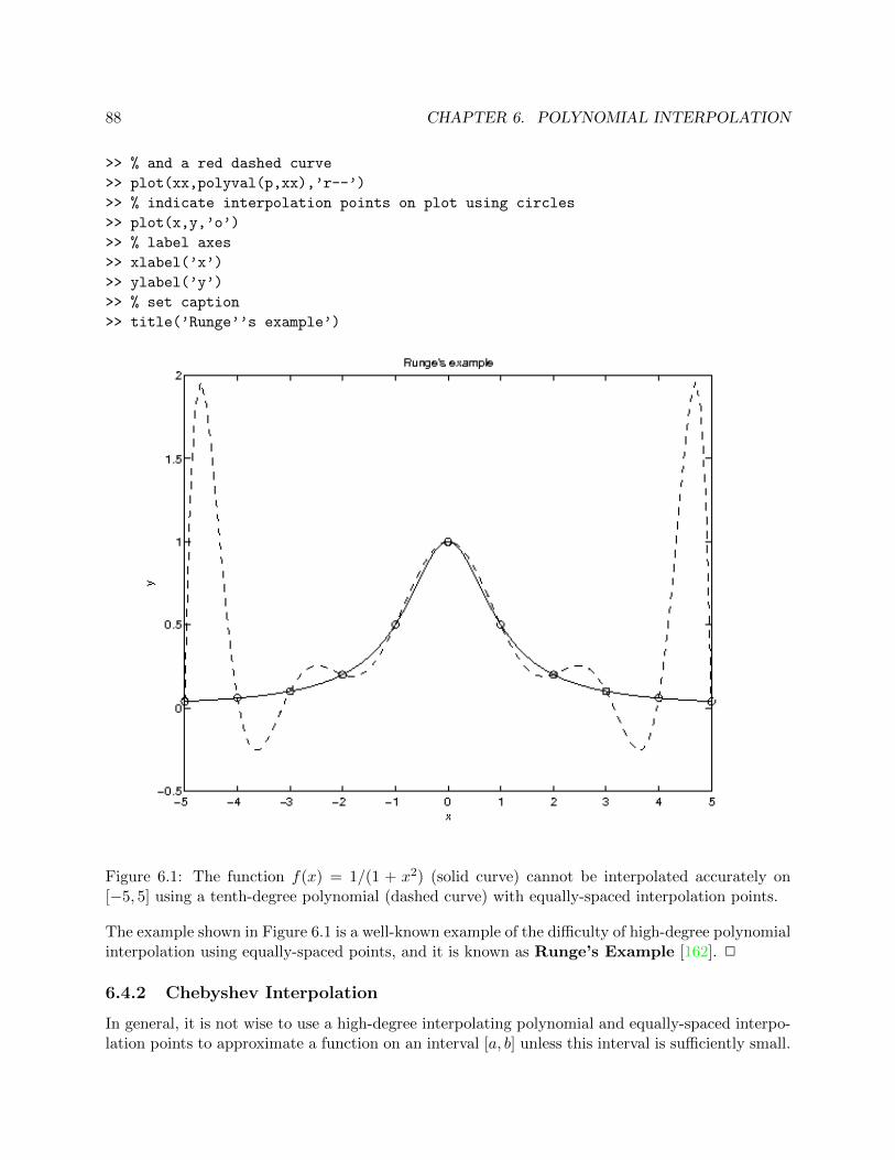
88 CHAPTER 6. POLYNOMIAL INTERPOLATION
>> % and a red dashed curve
>> plot(xx,polyval(p,xx),’r--’)
>> % indicate interpolation points on plot using circles
>> plot(x,y,’o’)
>> % label axes
>> xlabel(’x’)
>> ylabel(’y’)
>> % set caption
>> title(’Runge’’s example’)
Figure 6.1: The function f(x) = 1/(1 + x2) (solid curve) cannot be interpolated accurately on[−5, 5] using a tenth-degree polynomial (dashed curve) with equally-spaced interpolation points.
The example shown in Figure 6.1 is a well-known example of the difficulty of high-degree polynomialinterpolation using equally-spaced points, and it is known as Runge’s Example [162]. 2
6.4.2 Chebyshev Interpolation
In general, it is not wise to use a high-degree interpolating polynomial and equally-spaced interpo-lation points to approximate a function on an interval [a, b] unless this interval is sufficiently small.
6.4. ERROR ANALYSIS 89
Is it possible to choose the interpolation points so that the error is minimized? To answer thisquestion, we introduce the Chebyshev polynomials
Tk(x) = cos(k cos−1(x)), |x| ≤ 1, k = 0, 1, 2, . . . . (6.13)
Using (6.13) and the sum and difference formulas for cosine,
cos(A+B) = cosA cosB − sinA sinB, (6.14)
cos(A−B) = cosA cosB + sinA sinB, (6.15)
it can be shown that the Chebyshev polynomials satisfy the three-term recurrence relation
Tk+1(x) = 2xTk(x)− Tk−1(x), k ≥ 1. (6.16)
It can easily be seen from this relation, and the first two Chebyshev polynomials, that Tk(x) is infact a polynomial for all integers k ≥ 0.
The Chebyshev polynomials have the following properties of interest:
1. The leading coefficient of Tk(x) is 2k−1.
2. Tk(x) is an even function if k is even, and an odd function if k is odd.
3. The zeros of Tk(x), for k ≥ 1, are
xj = cos(2j + 1)π
2k, j = 0, 1, 2, . . . , k − 1.
These roots are known as the Chebyshev points. Because these points are cosines of equallyspaced angles in (0, π), they are distributed non-uniformly within (−1, 1). In particular, thepoints become closely clustered near the endpoints x = ±1.
4. The extrema of Tk(x) on [−1, 1] are
xj = cosjπ
k, j = 0, 1, . . . , k,
and the corresponding extremal values are ±1.
5. |Tk(x)| ≤ 1 on [−1, 1] for all k ≥ 0.
Exploration 6.4.3 Use (6.13), (6.14), and (6.15) to prove (6.16).
Exploration 6.4.4 Use (6.16) and induction to show that the leading coefficient of Tk(x)is 2k−1, for k ≥ 1.
Exploration 6.4.5 Use the roots of cosine to compute the roots of Tk(x). Show thatthey are real, distinct, and lie within (−1, 1).
90 CHAPTER 6. POLYNOMIAL INTERPOLATION
Let f(x) be a function that is (n+1) times continuously differentiable on [a, b]. If we approximatef(x) by a nth-degree polynomial pn(x) that interpolates f(x) at the n+ 1 roots of the Chebyshevpolynomial Tn+1(x), mapped from [−1, 1] to [a, b],
ξj =1
2(b− a) cos
(2j + 1)π
2n+ 2+
1
2(a+ b),
then the error in this approximation is
f(x)− pn(x) =f (n+1)(ξ)
(n+ 1)!
(b− a
2
)n+1
2−nTn+1(t(x)),
where
t(x) = −1 +2
b− a(x− a)
is the linear map from [a, b] to [−1, 1]. This is because
n∏j=0
(x− ξj) =
(b− a
2
)n+1 n∏j=0
(t(x)− τj) =
(b− a
2
)n+1
2−nTn+1(t(x)),
where τj is the jth root of Tn+1(t). From |Tn+1(t)| ≤ 1, we obtain
|f(x)− pn(x)| ≤ (b− a)n+1
22n+1(n+ 1)!maxξ∈[a,b]
|f (n+1)(ξ)|.
It can be shown that using Chebyshev points leads to much less error in the function f(x) =1/(1 + x2) from Runge’s example [154].
6.4.3 Concept Check
1. What is the error in the interpolating polynomial pn(x) of degree n that is used to interpolatef(x) at the points x0, x1, . . . , xn?
2. What is Runge’s example and what is its significance?
3. What is a Chebyshev polynomial?
4. What is the three-term recurrence relation satisfied by the Chebyshev polynomials?
5. What are Chebyshev points? How are they distributed?
6. What is the benefit of using Chebyshev points for polynomial interpolation?
6.5 Osculatory Interpolation
Suppose that the interpolation points are perturbed so that two neighboring points xi and xi+1,0 ≤ i < n, approach each other. What happens to the interpolating polynomial? In the limit, asxi+1 → xi, the interpolating polynomial pn(x) not only satisfies pn(xi) = yi, but also the condition
p′n(xi) = limxi+1→xi
yi+1 − yixi+1 − xi
.

6.5. OSCULATORY INTERPOLATION 91
It follows that in order to ensure uniqueness, the data must specify the value of the derivative ofthe interpolating polynomial at xi.
In general, the inclusion of an interpolation point xi k times within the set x0, . . . , xn must be
accompanied by specification of p(j)n (xi), j = 0, . . . , k − 1, in order to ensure a unique solution.
These values, divided by j!, are used in place of divided differences of identical interpolation pointsin Newton interpolation.
Interpolation with repeated interpolation points is called osculatory interpolation, since itcan be viewed as the limit of distinct interpolation points approaching one another, and the term“osculatory” is based on the Latin word for “kiss”.
Exploration 6.5.1 Use a divided-difference table to compute the interpolating polyno-mial p2(x) for the function f(x) = cosx on [0, π], with interpolation points x0 = x1 = 0and x2 = π. That is, p2(x) must satisfy p2(0) = f(0), p′2(0) = f ′(0) and p2(π) = f(π).Then, extend p2(x) to a cubic polynomial p3(x) by also requiring that p′3(π) = f ′(π),updating the divided-difference table accordingly.
Exploration 6.5.2 Suppose that osculatory interpolation is used to construct the poly-nomial pn(x) that interpolates f(x) at only one x-value, x0, and satisfies pn(x0) = f(x0),
p′n(x0) = f ′(x0), p′′n(x0) = f ′′(x0), and so on, up to p(n)n (x0) = f (n)(x0). What polynomial
approximation of f(x) is obtained?
6.5.1 Hermite Interpolation
In the case where each of the interpolation points x0, x1, . . . , xn is repeated exactly once, theinterpolating polynomial for a differentiable function f(x) is called the Hermite polynomial off(x), and is denoted by H2n+1(x), since this polynomial must have degree 2n+1 in order to satisfythe 2n+ 2 constraints
H2n+1(xi) = f(xi), H ′2n+1(xi) = f ′(xi), i = 0, 1, . . . , n.
To satisfy these constraints, we define, for i = 0, 1, . . . , n,
H2n+1,i(x) = [Ln,i(x)]2(1− 2L′n,i(xi)(x− xi)), (6.17)
K2n+1,i(x) = [Ln,i(x)]2(x− xi), (6.18)
where, as before, Ln,i(x) is the ith Lagrange polynomial for the interpolation points x0, x1, . . . , xn.It can be verified directly that these polynomials satisfy, for i, j = 0, 1, . . . , n,
H2n+1,i(xj) = δij , H′2n+1,i(xj) = 0,
K2n+1,i(xj) = 0, K′2n+1,i(xj) = δij ,
where δij is the Kronecker delta
δij =
1 i = j0 i 6= j
.
It follows that
H2n+1(x) =
n∑i=0
[f(xi)H2n+1,i(x) + f ′(xi)K2n+1,i(x)]
92 CHAPTER 6. POLYNOMIAL INTERPOLATION
is a polynomial of degree 2n+ 1 that satisfies the above constraints.
Exploration 6.5.3 Derive the formulas (6.17), (6.18) for H2n+1,i(x) and K2n+1,i(x),respectively, using the specified constraints for these polynomials. Hint: use an approachsimilar to that used to derive the formula for Lagrange polynomials.
To prove that this polynomial is the unique polynomial of degree 2n+ 1, we assume that thereis another polynomial H2n+1 of degree 2n + 1 that satisfies the constraints. Because H2n+1(xi) =H2n+1(xi) = f(xi) for i = 0, 1, . . . , n, H2n+1−H2n+1 has at least n+1 zeros. It follows from Rolle’sTheorem that H ′2n+1−H ′2n+1 has n zeros that lie within the intervals (xi−1, xi) for i = 0, 1, . . . , n−1.
Furthermore, becauseH ′2n+1(xi) = H ′2n+1(xi) = f ′(xi) for i = 0, 1, . . . , n, it follows thatH ′2n+1−H ′2n+1 has n + 1 additional zeros, for a total of at least 2n + 1. However, H ′2n+1 − H ′2n+1 is apolynomial of degree 2n, and the only way that a polynomial of degree 2n can have 2n + 1 zerosis if it is identically zero. Therefore, H2n+1 − H2n+1 is a constant function, but since this functionis known to have at least n + 1 zeros, that constant must be zero, and the Hermite polynomial isunique.
Using a similar approach as for the Lagrange interpolating polynomial, the following result canbe proved.
Theorem 6.5.1 Let f be 2n+2 times continuously differentiable on [a, b], and let H2n+1
denote the Hermite polynomial of f with interpolation points x0, x1, . . . , xn in [a, b]. Thenthere exists a point ξ(x) ∈ [a, b] such that
f(x)−H2n+1(x) =f (2n+2)(ξ(x))
(2n+ 2)!(x− x0)2(x− x1)2 · · · (x− xn)2.
The proof will be left as an exercise.
6.5.2 Divided Differences
The Hermite polynomial can be described using Lagrange polynomials and their derivatives, butthis representation is not practical because of the difficulty of differentiating and evaluating thesepolynomials. Instead, one can construct the Hermite polynomial using a divided-difference table, asdiscussed previously, in which each entry corresponding to two identical interpolation points is filledwith the value of f ′(x) at the common point. Then, the Hermite polynomial can be representedusing the Newton divided-difference formula.
Example 6.5.2 We will use Hermite interpolation to construct the third-degree polynomial H3(x)that fits f(x) and f ′(x) at x0 = 0 and x1 = 1. For convenience, we define new interpolation pointszi that list each (distinct) x-value twice:
z2i = z2i+1 = xi, i = 0, 1, . . . , n.
Our data is as follows:
i zi f(zi) f ′(zi)
0,1 0 0 12,3 1 0 1
6.5. OSCULATORY INTERPOLATION 93
In other words, we must have H3(0) = 0, H ′3(0) = 1, H3(1) = 0, and H ′3(1) = 1. To includethe values of f ′(x) at the two distinct interpolation points, we repeat each point once, so thatthe number of interpolation points, including repetitions, is equal to the number of constraintsdescribed by the data.
First, we construct the divided-difference table from this data. The divided differences in thetable are computed as follows:
f [z0] = f(z0) = 0, f [z1] = f(z1) = 0, f [z2] = f(z2) = 0, f [z3] = f(z3) = 0,
f [z0, z1] =f [z1]− f [z0]
z1 − z0
= f ′(z0)
= 1
f [z1, z2] =f [z2]− f [z1]
z2 − z1
=0− 0
1− 0= 0
f [z2, z3] =f [z3]− f [z2]
z3 − z2
= f ′(z2)
= 1
f [z0, z1, z2] =f [z1, z2]− f [z0, z1]
z2 − z0
=0− 1
1− 0= −1
f [z1, z2, z3] =f [z2, z3]− f [z1, z2]
z3 − z1
=1− 0
1− 0= 1
f [z0, z1, z2, z3] =f [z1, z2, z3]− f [z0, z1, z2]
z3 − z0
=1− (−1)
1− 0= 2
Note that the values of the derivative are used whenever a divided difference of the form f [zi, zi+1]is to be computed, where zi = zi+1. This makes sense because
limzi+1→zi
f [zi, zi+1] = limzi+1→zi
f(zi+1)− f(zi)
zi+1 − zi= f ′(zi).
The resulting divided-difference table is
94 CHAPTER 6. POLYNOMIAL INTERPOLATION
z0 = 0 f [z0] = 0f [z0, z1] = 1
z1 = 0 f [z1] = 0 f [z0, z1, z2] = −1f [z1, z2] = 0 f [z0, z1, z2, z3] = 2
z2 = 1 f [z2] = 0 f [z1, z2, z3] = 1f [z2, z3] = 1
z3 = 1 f [z3] = 0
It follows that the interpolating polynomial p3(x) can be obtained using the Newton divided-difference formula as follows:
H3(x) =3∑j=0
f [z0, . . . , zj ]
j−1∏i=0
(x− zi)
= f [z0] + f [z0, z1](x− z0) + f [z0, z1, z2](x− z0)(x− z1) +
f [z0, z1, z2, z3](x− z0)(x− z1)(x− z2)
= 0 + (x− 0) + (−1)(x− 0)(x− 0) + 2(x− 0)(x− 0)(x− 1)
= x− x2 + 2x2(x− 1).
We see that Hermite interpolation, using divided differences, produces an interpolating polynomialthat is in the Newton form, with centers z0 = 0, z1 = 0, and z2 = 1. 2
Exploration 6.5.4 Use the Newton form of the Hermite interpolating polynomial toprove Theorem 6.5.1.
Exploration 6.5.5 Modify your function divdiffs from Exploration 6.3.6 to obtain anew function c=hermdivdiffs(x,y,yp) that computes the divided difference table fromthe given data stored in the input vectors x and y, as well as the derivative valuesstored in yp, and returns a vector c consisting of the divided differences f [z0, . . . , zj ],j = 0, 1, 2, . . . , 2n+ 1, where n+ 1 is the length of both x and y.
Exploration 6.5.6 Write a Matlab function H=hermpolyfit(x,y,yp) that is similarto the built-in function polyfit, in that it returns a vector of coefficients, in power form,for the interpolating polynomial corresponding to the given data, except that Hermiteinterpolation is used instead of Lagrange interpolation. Use the function hermdivdiffs
from Exploration 6.5.5 as well as the function powerform from Exploration 6.3.8.
6.5.3 Concept Check
1. What is osculatory interpolation?
2. When interpolation points are repeated, how is uniqueness of the interpolating polynomialensured?
3. What is Hermite interpolation?
4. What is the error in the Hermite interpolating polynomial H2n+1(x) that interpolates f(x)at the points x0, x1, . . . , xn?
6.6. PIECEWISE POLYNOMIAL INTERPOLATION 95
5. How is a divided difference table useful for computing a Hermite interpolating polynomial?
6.6 Piecewise Polynomial Interpolation
We have seen that high-degree polynomial interpolation can be problematic. However, if the fittingfunction is only required to have a few continuous derivatives, then one can construct a piecewisepolynomial to fit the data. We now precisely define what we mean by a piecewise polynomial.
Definition 6.6.1 (Piecewise polynomial) Let [a, b] be an interval that is divided intosubintervals [xi, xi+1], where i = 0, . . . , n− 1, x0 = a and xn = b. A piecewise polyno-mial is a function p(x) defined on [a, b] by
p(x) = pi(x), xi−1 ≤ x ≤ xi, i = 1, 2, . . . , n,
where, for i = 1, 2, . . . , n, each function pi(x) is a polynomial defined on [xi−1, xi]. Thedegree of p(x) is the maximum degree of each polynomial pi(x), for i = 1, 2, . . . , n.
It is essential to note that by this definition, a piecewise polynomial defined on [a, b] is equal tosome polynomial on each subinterval [xi−1, xi] of [a, b], for i = 1, 2, . . . , n, but a different polynomialmay be used for each subinterval.
To study the accuracy of piecewise polynomials, we need to work with various function spaces,including Sobolev spaces; these function spaces are defined in Section B.12.3.
6.6.1 Piecewise Linear Approximation
We first consider one of the simplest types of piecewise polynomials, a piecewise linear polynomial.Let f ∈ C[a, b]. Given the points x0, x1, . . . , xn defined as above, the linear spline sL(x) thatinterpolates f at these points is defined by
sL(x) = f(xi−1)x− xixi−1 − xi
+ f(xi)x− xi−1
xi − xi−1, x ∈ [xi−1, xi], i = 1, 2, . . . , n. (6.19)
The points x0, x1, . . . , xn are the knots of the spline.
Exploration 6.6.1 Given that sL(x) must satisfy sL(xi) = f(xi) for i = 0, 1, 2, . . . , n,explain how the formula (6.19) can be derived.
Exploration 6.6.2 Given the points (x0, f(x0)), (x1, f(x1)), . . . , (xn, f(xn)) plotted inthe xy-plane, explain how sL can easily be graphed. How can the graph be produced in asingle line of Matlab code, given vectors x and y containing the x- and y- coordinatesof these points, respectively?
If f ∈ C2[a, b], then by the error in Lagrange interpolation (Theorem 6.4.1), on each subinterval[xi−1, xi], for i = 1, 2, . . . , n, we have
f(x)− sL(x) =f ′′(ξ)
2(x− xi−1)(x− xi).
This leads to the following Theorem.

96 CHAPTER 6. POLYNOMIAL INTERPOLATION
Theorem 6.6.2 Let f ∈ C2[a, b], and let sL be the piecewise linear spline defined by(6.19). For i = 1, 2, . . . , n, let hi = xi − xi−1, and define h = max1≤i≤n hi. Then
‖f − sL‖∞ ≤M
8h2,
where |f ′′(x)| ≤M on [a, b].
Exploration 6.6.3 Prove Theorem 6.6.2.
In Section 6.4, it was observed in Runge’s example that even when f(x) is smooth, an inter-polating polynomial of f(x) can be highly oscillatory, depending on the number and placement ofinterpolation points. By contrast, one of the most welcome properties of the linear spline sL(x)is that among all functions in H1(a, b) that interpolate f(x) at the knots x0, x1, . . . , xn, it is the“flattest”. That is, for any function v ∈ H1(a, b) that interpolates f at the knots,
‖s′L‖2 ≤ ‖v′‖2.
To prove this, we first write
‖v′‖22 = ‖v′ − s′L‖22 + 2〈v′ − s′L, s′L〉+ ‖s′L‖22.
We then note that on each subinterval [xi−1, xi], since sL is a linear function, s′L is a constantfunction, which we denote by
sL(x) ≡ mi =f(xi)− f(xi−1)
xi − xi−1, i = 1, 2, . . . , n.
We then have
〈v′ − s′L, s′L〉 =
∫ b
a[v′(x)− s′L(x)]s′L(x) dx
=n∑i=1
∫ xi
xi−1
[v′(x)− s′L(x)]s′L(x) dx
=n∑i=1
mi
∫ xi
xi−1
v′(x)−mi dx
=
n∑i=1
mi [v(x)−mix]|xixi−1
=
n∑i=1
mi
[v(xi)− v(xi−1)− f(xi)− f(xi−1)
xi − xi−1(xi − xi−1)
]= 0,
because by assumption, v(x) interpolates f(x) at the knots. This leaves us with
‖v′‖22 = ‖v′ − s′L‖22 + ‖s′L‖22,
which establishes the result.
6.6. PIECEWISE POLYNOMIAL INTERPOLATION 97
6.6.2 Cubic Spline Interpolation
A major drawback of the linear spline is that it does not have any continuous derivatives. Thisis significant when the function to be approximated, f(x), is a smooth function. Therefore, itis desirable that a piecewise polynomial approximation possess a certain number of continuousderivatives. This requirement imposes additional constraints on the piecewise polynomial, andtherefore the degree of the polynomials used on each subinterval must be chosen sufficiently highto ensure that these constraints can be satisfied.
We therefore define a spline of degree k to be a piecewise polynomial of degree k that has k−1continuous derivatives. The most commonly used spline is a cubic spline, which we now define.
Definition 6.6.3 (Cubic Spline) Let f(x) be function defined on an interval [a, b], andlet x0, x1, . . . , xn be n + 1 distinct points in [a, b], where a = x0 < x1 < · · · < xn = b. Acubic spline, or cubic spline interpolant, is a piecewise polynomial s(x) that satisfiesthe following conditions:
1. On each interval [xi−1, xi], for i = 1, . . . , n, s(x) = si(x), where si(x) is a cubicpolynomial.
2. s(xi) = f(xi) for i = 0, 1, . . . , n.
3. s(x) is twice continuously differentiable on (a, b).
4. Either of the following boundary conditions are satisfied:
(a) s′′(a) = s′′(b) = 0, which is called free or natural boundary conditions,and
(b) s′(a) = f ′(a) and s′(b) = f ′(b), which is called clamped boundary condi-tions.
If s(x) satisfies free boundary conditions, we say that s(x) is a natural spline. Thepoints x0, x1, . . . , xn are called the nodes of s(x).
Clamped boundary conditions are often preferable because they use more information about f(x),which yields a spline that better approximates f(x) on [a, b]. However, if information about f ′(x)is not available, then natural boundary conditions must be used instead.
6.6.2.1 Constructing Cubic Splines
Suppose that we wish to construct a cubic spline interpolant s(x) that fits the given data (x0, y0),(x1, y1), . . . , (xn, yn), where a = x0 < x1 < · · · < xn = b, and yi = f(xi), for some known functionf(x) defined on [a, b]. From the preceding discussion, this spline is a piecewise polynomial of theform
s(x) = si(x) = di(x− xi−1)3 + ci(x− xi−1)2 + bi(x− xi−1) + ai, i = 1, 2, . . . , n, xi−1 ≤ x ≤ xi.(6.20)
That is, the value of s(x) is obtained by evaluating a different cubic polynomial for each subinterval[xi−1, xi], for i = 1, 2, . . . , n.
98 CHAPTER 6. POLYNOMIAL INTERPOLATION
We now use the definition of a cubic spline to construct a system of equations that must besatisfied by the coefficients ai, bi, ci and di for i = 1, 2, . . . , n. We can then compute these coefficientsby solving the system. Because s(x) must fit the given data, we have
s(xi−1) = ai = yi−1 = f(xi−1), i = 1, 2, . . . , n. (6.21)
If we define hi = xi−xi−1, for i = 1, 2, . . . , n, and define an+1 = yn, then the requirement that s(x)is continuous at the interior nodes implies that we must have si(xi) = si+1(xi) for i = 1, 2, . . . , n−1.Furthermore, because s(x) must fit the given data, we must also have s(xn) = sn(xn) = yn. Theseconditions lead to the constraints
si(xi) = dih3i + cih
2i + bihi + ai = ai+1 = si+1(xi), i = 1, 2, . . . , n. (6.22)
To ensure that s(x) has a continuous first derivative at the interior nodes, we require thats′i(xi) = s′i+1(xi) for i = 1, 2 . . . , n− 1, which imposes the constraints
s′i(xi) = 3dih2i + 2cihi + bi = bi+1 = s′i+1(xi), i = 1, 2, . . . , n− 1. (6.23)
Similarly, to enforce continuity of the second derivative at the interior nodes, we require thats′′i (xi) = s′′i+1(xi) for i = 1, 2, . . . , n− 1, which leads to the constraints
s′′i (xi) = 6dihi + 2ci = 2ci+1 = s′′i+1(xi), i = 1, 2, . . . , n− 1. (6.24)
There are 4n coefficients to determine, since there are n cubic polynomials, with 4 coefficientseach. However, we have only prescribed 4n− 2 constraints, so we must specify 2 more in order todetermine a unique solution. If we use natural boundary conditions, then these constraints are
s′′1(x0) = 2c1 = 0, (6.25)
s′′n(xn) = 3dnhn + cn = 0. (6.26)
On the other hand, if we use clamped boundary conditions, then our additional constraints are
s′1(x0) = b1 = z0, (6.27)
s′n(xn) = 3dnh2n + 2cnhn + bn = zn, (6.28)
where zi = f ′(xi) for i = 0, 1, . . . , n.
Having determined our constraints that must be satisfied by s(x), we can set up a system of 4nlinear equations based on these constraints, and then solve this system to determine the coefficientsai, bi, ci, di for i = 1, 2 . . . , n.
However, it is not necessary to construct the matrix for such a system, because it is possibleto instead solve a smaller system of only O(n) equations obtained from the continuity conditions(6.23) and the boundary conditions (6.25), (6.26) or (6.27), (6.28), depending on whether naturalor clamped boundary conditions, respectively, are imposed. This reduced system is accomplishedby using equations (6.21), (6.22) and (6.24) to eliminate the ai, bi and di, respectively.

6.6. PIECEWISE POLYNOMIAL INTERPOLATION 99
Exploration 6.6.4 Show that under natural boundary conditions, the coefficientsc2, . . . , cn of the cubic spline (6.20) satisfy the system of equations Ac = b, where
A =
2(h1 + h2) h2 0 · · · 0
h2 2(h2 + h3) h3. . .
...
0. . .
. . .. . . 0
.... . .
. . .. . . hn−1
0 · · · 0 hn−1 2(hn−1 + hn)
,
c =
c2...cn
, b =
3h2
(a3 − a2)− 3h1
(a2 − a1)...
3hn
(an+1 − an)− 3hn−1
(an − an−1)
.Exploration 6.6.5 Show that under clamped boundary conditions, the coefficientsc1, . . . , cn+1 of the cubic spline (6.20) satisfy the system of equations Ac = b, where
A =
2h1 h1 0 · · · · · · 0
h1 2(h1 + h2) h2. . .
...
0 h2 2(h2 + h3) h3. . .
......
. . .. . .
. . .. . . 0
.... . . hn−1 2(hn−1 + hn) hn
0 · · · · · · 0 hn 2hn
,
c =
c1
c2...
cn+1
, b =
3h1
(a2 − a1)− 3z03h2
(a3 − a2)− 3h1
(a2 − a1)...
3hn
(an+1 − an)− 3hn−1
(an − an−1)
3zn − 3hn
(an+1 − an)
,
and cn+1 = s′′n(xn).
Example 6.6.4 We will construct a cubic spline interpolant for the following data on the interval[0, 2].
j xj yj0 0 31 1/2 −42 1 53 3/2 −64 2 7
The spline, s(x), will consist of four pieces sj(x)4j=1, each of which is a cubic polynomial of the
100 CHAPTER 6. POLYNOMIAL INTERPOLATION
formsj(x) = aj + bj(x− xj−1) + cj(x− xj−1)2 + dj(x− xj−1)3, j = 1, 2, 3, 4.
We will impose natural boundary conditions on this spline, so it will satisfy the conditions s′′(0) =s′′(2) = 0, in addition to the “essential” conditions imposed on a spline: it must fit the given dataand have continuous first and second derivatives on the interval [0, 2].
These conditions lead to the following system of equations that must be solved for the coefficientsc1, c2, c3, c4, and c5, where cj = s′′(xj−1)/2 for j = 1, 2, . . . , 5. We define h = (2− 0)/4 = 1/2 to bethe spacing between the interpolation points.
c1 = 0h
3(c1 + 4c2 + c3) =
y2 − 2y1 + y0
hh
3(c2 + 4c3 + c4) =
y3 − 2y2 + y1
hh
3(c3 + 4c4 + c5) =
y4 − 2y3 + y2
hc5 = 0.
Substituting h = 1/2 and the values of yj , and also taking into account the boundary conditions,we obtain
1
6(4c2 + c3) = 32
1
6(c2 + 4c3 + c4) = −40
1
6(c3 + 4c4) = 48
This system has the solutions
c2 = 516/7, c3 = −720/7, c4 = 684/7.
Using (6.21), (6.22), and (6.24), we obtain
a1 = 3, a2 = −4, a3 = 5, a4 = −6.
b1 = −184/7, b2 = 74/7, b3 = −4, b4 = −46/7,
andd1 = 344/7, d2 = −824/7, d3 = 936/7, d4 = −456/7.
We conclude that the spline s(x) that fits the given data, has two continuous derivatives on [0, 2],and satisfies natural boundary conditions is
s(x) =
3447 x3 − 184
7 x2 + 3 if x ∈ [0, 0.5]−824
7 (x− 1/2)3 + 5167 (x− 1/2)2 + 74
7 (x− 1/2)− 4 if x ∈ [0.5, 1]9367 (x− 1)3 − 720
7 (x− 1)2 − 4(x− 1) + 5 if x ∈ [1, 1.5]−456
7 (x− 3/2)3 + 6847 (x− 3/2)2 − 46
7 (x− 3/2)− 6 if x ∈ [1.5, 2]
.
The graph of the spline is shown in Figure 6.2. 2
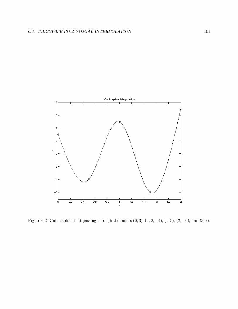
6.6. PIECEWISE POLYNOMIAL INTERPOLATION 101
Figure 6.2: Cubic spline that passing through the points (0, 3), (1/2,−4), (1, 5), (2,−6), and (3, 7).
102 CHAPTER 6. POLYNOMIAL INTERPOLATION
The Matlab function spline can be used to construct cubic splines satisfying both natural(also known as “not-a-knot”) and clamped boundary conditions. The following exercises requirereading the documentation for this function.
Exploration 6.6.6 Use spline to construct a cubic spline for the data from Example6.6.4. First, use the interface pp=spline(x,y), where x and y are vectors consistingof the x- and y-coordinates, respectively, of the given data points, and pp is a structurethat represents the cubic spline s(x). Examine the members of p and determine how tointerpret them. Where do you see the coefficients computed in Example 6.6.4?
Exploration 6.6.7 The interface yy=spline(x,y,xx), where xx is a vector of x-valuesat which the spline constructed from x and y should be evaluated, produces a vector yy ofcorresponding y-values. Use this interface on the data from Example 6.6.4 to reproduceFigure 6.2.
Exploration 6.6.8 Use polyder and polyval to plot the first and second derivatives ofthe cubic spline computed in Exploration 6.6.6 to confirm that they are in fact continuous.Note: be careful about the choice of x-values at which each piece is evaluated!
Exploration 6.6.9 If the input argument y in the function call pp=spline(x,y) has twocomponents more than x, it is assumed that the first and last components are the slopesz0 = s′(x0) and zn = s′(xn) imposed by clamped boundary conditions. Use the given datafrom Example 6.6.4, with various values of z0 and zn, and construct the clamped cubicspline using this interface to spline. Compare the coefficients and graphs to that of thenatural cubic spline from Explorations 6.6.6 and 6.6.7.
6.6.2.2 Well-Posedness and Accuracy
For both sets of boundary conditions, the system Ac = b has a unique solution, because thematrix A is strictly row diagonally dominant. This property guarantees that A is invertible, dueto Gerschgorin’s Circle Theorem. We therefore have the following results.
Theorem 6.6.5 Let x0, x1, . . . , xn be n + 1 distinct points in the interval [a, b], wherea = x0 < x1 < · · · < xn = b, and let f(x) be a function defined on [a, b]. Then fhas a unique cubic spline interpolant s(x) that is defined on the nodes x0, x1, . . . , xn thatsatisfies the natural boundary conditions s′′(a) = s′′(b) = 0.
Theorem 6.6.6 Let x0, x1, . . . , xn be n + 1 distinct points in the interval [a, b], wherea = x0 < x1 < · · · < xn = b, and let f(x) be a function defined on [a, b] that isdifferentiable at a and b. Then f has a unique cubic spline interpolant s(x) that is definedon the nodes x0, x1, . . . , xn that satisfies the clamped boundary conditions s′(a) = f ′(a)and s′(b) = f ′(b).
Just as the linear spline is the “flattest” interpolant, in an average sense, the natural cubic splinehas the least “average curvature”. Specifically, if s2(x) is the natural cubic spline for f ∈ C[a, b] on[a, b] with knots a = x0 < x1 < · · · < xn = b, and v ∈ H2(a, b) is any interpolant of f with these
6.6. PIECEWISE POLYNOMIAL INTERPOLATION 103
knots, then
‖s′′2‖2 ≤ ‖v′′‖2.
This can be proved in the same way as the corresponding result for the linear spline. It is thisproperty of the natural cubic spline, called the smoothest interpolation property, from whichsplines were named.
The following result, proved in [165, p. 57-58], provides insight into the accuracy with which acubic spline interpolant s(x) approximates a function f(x).
Theorem 6.6.7 Let f be four times continuously differentiable on [a, b], and assumethat ‖f (4)‖∞ = M . Let s(x) be the unique clamped cubic spline interpolant of f(x) onthe nodes x0, x1, . . . , xn, where a = x0 < x1 < · · · < xn < b. Then for x ∈ [a, b],
‖f(x)− s(x)‖∞ ≤5M
384max
1≤i≤nh4i ,
where hi = xi − xi−1.
A similar result applies in the case of natural boundary conditions [20].
6.6.2.3 Hermite Cubic Splines
We have seen that it is possible to construct a piecewise cubic polynomial that interpolates afunction f(x) at knots a = x0 < x1 < · · · < xn = b, that belongs to C2[a, b]. Now, suppose thatwe also know the values of f ′(x) at the knots. We wish to construct a piecewise cubic polynomials(x) that agrees with f(x), and whose derivative agrees with f ′(x) at the knots. This piecewisepolynomial is called a Hermite cubic spline.
Because s(x) is cubic on each subinterval [xi−1, xi] for i = 1, 2, . . . , n, there are 4n coefficients,and therefore 4n degrees of freedom, that can be used to satisfy any criteria that are imposed ons(x). Requiring that s(x) interpolates f(x) at the knots, and that s′(x) interpolates f ′(x) at theknots, imposes 2n+2 constraints on the coefficients. We can then use the remaining 2n−2 degreesof freedom to require that s(x) belong to C1[a, b]; that is, it is continuously differentiable on [a, b].Note that unlike the cubic spline interpolant, the Hermite cubic spline does not have a continuoussecond derivative.
The following result provides insight into the accuracy with which a Hermite cubic spline inter-polant s(x) approximates a function f(x).
Theorem 6.6.8 Let f be four times continuously differentiable on [a, b], and assume that‖f (4)‖∞ = M . Let s(x) be the unique Hermite cubic spline interpolant of f(x) on thenodes x0, x1, . . . , xn, where a = x0 < x1 < · · · < xn < b. Then
‖f(x)− s(x)‖∞ ≤M
384max
1≤i≤nh4i ,
where hi = xi − xi−1.
This can be proved in the same way as the error bound for the linear spline, except that the errorformula for Hermite interpolation is used instead of the error formula for Lagrange interpolation.
104 CHAPTER 6. POLYNOMIAL INTERPOLATION
Exploration 6.6.10 Prove Theorem 6.6.8.
An advantage of Hermite cubic splines over cubic spline interpolants is that they are localapproximations rather than global; that is, if the values of f(x) and f ′(x) change at some knotxi, only the polynomials defined on the pieces containing xi need to be changed. In cubic splineinterpolation, all pieces are coupled, so a change at one point changes the polynomials for all pieces.
To see this, we represent the Hermite cubic spline using the same form as in the cubic splineinterpolant,
si(x) = ai + bi(x− xi−1) + ci(x− xi−1)2 + di(x− xi−1)3, x ∈ [xi−1, xi], (6.29)
for i = 1, 2, . . . , n. Then, the coefficients ai, bi, ci, di can be determined explicitly in terms of onlyf(xi−1), f ′(xi−1), f(xi) and f ′(xi).
Exploration 6.6.11 Use the conditions
si(xi−1) = f(xi−1), si(xi) = f(xi), s′i(xi−1) = f ′(xi−1), s′i(xi) = f ′(xi)
to obtain the values of the coefficients ai, bi, ci, di in (6.29).
Exploration 6.6.12 Write a Matlab function hp=hermitespline(x,y) that con-structs a Hermite cubic spline for the data given in the vectors x and y. The outputhp should be a structure that contains enough information so that the spline can be eval-uated at any x-value without having to specify any additional parameters. Write a secondfunction y=hsplineval(hp,x) that performs this evaluation.
6.6.3 Concept Check
1. What is piecewise polynomial interpolation?
2. What shortcoming of polynomial interpolation does piecewise polynomial interpolation ad-dress?
3. Describe one advantage and one disadvantage of piecewise linear interpolation.
4. What does it mean to say that a linear spline is the “flattest” interpolant?
5. What are the properties of a cubic spline?
6. Why are boundary conditions required for a cubic spline?
7. Describe two types of boundary conditions that can be imposed on a cubic spline.
8. How does cubic spline interpolation compare to Lagrange interpolation in terms of efficiency?
9. What is the “smoothest interpolation property” of cubic splines?
10. How are cubic splines computed in Matlab?

6.7. ADDITIONAL RESOURCES 105
6.7 Additional Resources
Polynomial interpolation is one of the most essential topics in numerical analysis, as it servesas the foundation of methods for numerical differentiation, numerical integration, certain time-stepping methods for ODEs, among others, as we will see later in this book. As such, polynomialinterpolation is covered quite thoroughly in other textbooks; in particular we call the reader’sattention to Ascher and Greif [8], Burden and Faires [31], Cheney and Kincaid [33], and Conteand de Boor [35]. Lagrange interpolation is covered in depth in [7, 10, 42]. Also covered in[7] is the use of Newton interpolation to efficiently update the interpolating polynomial for ENO(“essentially non-oscillatory”) schemes for differential equations. A textbook by Davis [41] providesa comprehensive reference on interpolation.
Books by Fox and Parker [67] and Rivlin [159] are devoted to Chebyshev polynomials. Trefethen,et al. have developed chebfun, an open-source Matlab toolbox for performing operations on func-tions, such as differentiation, integration, and solution of differential equations, in which functionsare represented internally by their Chebyshev interpolants. The methods of chebfun take advantageof the fact that accurate high-degree polynomial interpolation is feasible when Chebyshev pointsare used as interpolation points. The chebfun toolbox is available at http://www.chebfun.org,and documentation is provided in [55].
The theory of splines is covered in books by Ahlberg, et al. [2], Knott [110], and Schumaker[166]. Texts that focus on the computational aspects, including software, are those by de Boor [44],Dierckx [47], Shikin and Plis [169], and Spath [172]. The application of splines to computer graphicsand geometric modeling is covered in books by Bartels, et al. [14], Farin [62], and Yamaguchi [204].Beyond the scope of this text is B-splines, which are basis functions used to describe cubic splines.Coverage of this topic can be found in [8, 44, 182]. Also presented in [8] is multi-dimensionalinterpolation, including with radial basis functions (RBFs).
6.8 Exercises
1. Compute, by hand, the Lagrange and Newton forms of the interpolating polynomial p3(x) ofdegree three for f(x) = x4 with interpolation points xi = i for i = 0, 1, 2, 3.
2. Compute, by hand, the Hermite interpolating polynomial h3(x) of degree three for f(x) = x4,with x0 = 0 and x1 = 3. Plot the graphs of f(x), p3(x) from Exercise 1, and h3(x) on thesame plot. Compare the accuracy of these two approximations.
3. Use Theorems 6.4.1 and 6.5.1 to obtain an upper bound for the error in the interpolatingpolynomials computed in Exercises 1 and 2 on [0, 3]. What step in this error estimationprocess is unnecessary if Chebyshev points are used as interpolation points? Explain why.
4. Describe, using pseudocode, an algorithm that evaluates a polynomial
pn(x) = a0 + a1x+ a2x2 + · · ·+ anx
n
at a given x-value by computing the terms of pn(x), as written above, from left to right,instead of using Horner’s Method. How many multiplications and additions are required?How does its efficiency compare to that of Horner’s Method?

106 CHAPTER 6. POLYNOMIAL INTERPOLATION
5. Given a polynomial pn(x) that interpolates the data (x0, y0), (x1, y1), . . ., (xn, yn), determinehow many additions and multiplications are required to evaluate pn(x) when it is in (a)Lagrange form, and (b) Newton form.
6. Show that the Lagrange polynomial Lj(x) defined in (6.2) can also be written as
Lj(x) =πn(x)
(x− xj)π′n(x),
where πn(x) = (x− x0)(x− x1)(x− x2) · · · (x− xn).
7. Consider a piecewise quadratic interpolant sQ(x) that interpolates a given function f(x) atx0, x1, . . . , xn, defined by
sQ(x) = si(x) = ai + bi(x− xi−1) + ci(x− xi−1)2, i = 1, 2, . . . , n.
How many continuous derivatives can sQ(x) be guaranteed to have? How many boundary con-ditions can be imposed? Describe a system of equations for obtaining the coefficients ai, bi, cifor i = 1, 2, . . . , n. Use boundary conditions analogous to clamped boundary conditions forcubic splines to ensure a unique solution.
8. Write your own Matlab functions that implement the built-in functions polyval, polyderand polyint. Use Horner’s Method to implement your version of polyval.
9. Write a Matlab function pp=clampedspline(x,y,spa,spb) that uses the system of equa-tions described in Exploration 6.6.5 to construct a cubic spline that interpolates the datadescribed by the vectors x and y and also satisfies clamped boundary conditions s′(a) = spa
and s′(b) = spb. The output p must be a structure similar to that returned by the built-inspline function that describes the computed spline.
10. We revisit the function from Runge’s Example
f(x) =1
1 + x2, −5 ≤ x ≤ 5.
Plot the graph of this function on the interval [−5, 5]. On the same plot, graph the followingapproximations:
(a) The Lagrange interpolating polynomial of f(x) of degree 10, with equally spaced inter-polation points xi = −5 + i, i = 0, 1, 2, . . . , 10.
(b) The Lagrange interpolating polynomial of f(x) of degree 10, with the Chebyshev pointsx0, x1, . . . , x10 equal to the roots of T10(x) mapped to the interval [−5, 5]
(c) A cubic spline that interpolates f(x) at the equally spaced points from part 10a.
Comment on the accuracy of these approximations.
Chapter 8
Differentiation and Integration
The solution of many mathematical models requires performing the basic operations of calculus,differentiation and integration. In this chapter, we will learn several techniques for approximating aderivative of a function at a point, and a definite integral of a function over an interval. As we willsee, our previous discussion of polynomial interpolation will play an essential role, as polynomialsare the easiest functions on which to perform these operations.
8.1 Numerical Differentiation
We first discuss how Taylor series and polynomial interpolation can be applied to help solve afundamental problem from calculus that frequently arises in scientific applications, the problem ofcomputing the derivative of a given function f(x) at a given point x = x0. The basics of derivativesare reviewed in Section A.2.
8.1.1 Derivation Using Taylor Series
Recall that the derivative of f(x) at a point x0, denoted f ′(x0), is defined by
f ′(x0) = limh→0
f(x0 + h)− f(x0)
h.
This definition suggests a method for approximating f ′(x0). If we choose h to be a small positiveconstant, then
f ′(x0) ≈ f(x0 + h)− f(x0)
h.
This approximation is called the forward difference formula.
To estimate the accuracy of this approximation, we note that if f ′′(x) exists on [x0, x0 + h],then, by Taylor’s Theorem, f(x0 +h) = f(x0)+f ′(x0)h+f ′′(ξ)h2/2, where ξ ∈ [x0, x0 +h]. Solvingfor f ′(x0), we obtain
f ′(x0) =f(x0 + h)− f(x0)
h− f ′′(ξ)
2h,
so the error in the forward difference formula is O(h). We say that this formula is first-orderaccurate.
107

108 CHAPTER 8. DIFFERENTIATION AND INTEGRATION
The forward-difference formula is called a finite difference approximation to f ′(x0), becauseit approximates f ′(x) using values of f(x) at points that have a small, but finite, distance betweenthem, as opposed to the definition of the derivative, that takes a limit and therefore computes thederivative using an “infinitely small” value of h. The forward-difference formula, however, is justone example of a finite difference approximation. If we replace h by −h in the forward-differenceformula, where h is still positive, we obtain the backward-difference formula
f ′(x0) ≈ f(x0)− f(x0 − h)
h.
Like the forward-difference formula, the backward difference formula is first-order accurate.If we average these two approximations, we obtain the centered difference formula
f ′(x0) ≈ f(x0 + h)− f(x0 − h)
2h.
To determine the accuracy of this approximation, we assume that f ′′′(x) exists on the interval[x0 − h, x0 + h], and then apply Taylor’s Theorem again to obtain
f(x0 + h) = f(x0) + f ′(x0)h+f ′′(x0)
2h2 +
f ′′′(ξ+)
6h3,
f(x0 − h) = f(x0)− f ′(x0)h+f ′′(x0)
2h2 − f ′′′(ξ−)
6h3,
where ξ+ ∈ [x0, x0 + h] and ξ− ∈ [x0 − h, x0]. Subtracting the second equation from the first andsolving for f ′(x0) yields
f ′(x0) =f(x0 + h)− f(x0 − h)
2h− f ′′′(ξ+) + f ′′′(ξ−)
12h2.
Suppose that f ′′′ is continuous on [x0−h, x0 +h]. By the Intermediate Value Theorem, f ′′′(x) mustassume every value between f ′′′(ξ−) and f ′′′(ξ+) on the interval (ξ−, ξ+), including the average ofthese two values. Therefore, we can simplify this equation to
f ′(x0) =f(x0 + h)− f(x0 − h)
2h− f ′′′(ξ)
6h2, (8.1)
where ξ ∈ [x0 − h, x0 + h]. Because the error is O(h2), we say that the centered-difference formulais second-order accurate. This is due to the cancellation of the terms involving f ′′(x0).
Example 8.1.1 Consider the function
f(x) =sin2
(√x2+x
cosx−x
)sin( √
x−1√x2+1
) .
Our goal is to compute f ′(0.25). Differentiating, using the Quotient Rule and the Chain Rule, weobtain
f ′(x) =2 sin
(√x2+x
cosx−x
)cos(√
x2+xcosx−x
) [2x+1
2√x2+1(cosx−x)
+√x2+1(sinx+1)(cosx−x)2
]sin( √
x−1√x2+1
) −
sin(√
x2+xcosx−x
)cos( √
x−1√x2+1
) [1
2√x√x2+1
− x(√x−1)
(x2+1)3/2
]sin2
( √x−1√x2+1
) .
8.1. NUMERICAL DIFFERENTIATION 109
Evaluating this monstrous function at x = 0.25 yields f ′(0.25) = −9.066698770.An alternative approach is to use a centered difference approximation,
f ′(x) ≈ f(x+ h)− f(x− h)
2h.
Using this formula with x = 0.25 and h = 0.005, we obtain the approximation
f ′(0.25) ≈ f(0.255)− f(0.245)
0.01= −9.067464295,
which has absolute error 7.7 × 10⁻⁴. While this complicated function must be evaluated twice toobtain this approximation, that is still much less work than using differentiation rules to computef ′(x), and then evaluating f ′(x), which is much more complicated than f(x). 2
Example 8.1.2 We will use Taylor expansion to derive an approximation of f ′(x0) of the form
f ′(x0) =1
h[c0f(x0) + c1f(x0 + h) + c2f(x0 + 2h)] + error. (8.2)
Such a formula is useful when there is no information available about f(x) for x < x0. The leadingfactor of 1/h is not essential, but it is used so that the coefficients c0, c1, c2 will be independent ofh. The Taylor expansions of f(x0 + h) and f(x0 + 2h) are
f(x0 + h) = f(x0) + f ′(x0)h+1
2f ′′(x0)h2 +
1
6f ′′′(ξ1)h3,
f(x0 + 2h) = f(x0) + f ′(x0)2h+1
2f ′′(x0)4h2 +
1
6f ′′′(ξ2)8h3,
where ξ1 ∈ [x0, x0 + h] and ξ2 ∈ [x0, x0 + 2h]. Substituting these expansions into (8.2), we see thatthe coefficients c0, c1 and c2 must satisfy the equations
c0 + c1 + c2 = 0,
c1 + 2c2 = 1,
c1 + 4c2 = 0.
This system of linear equations has the unique solution
c0 = −3
2, c1 = 2, c2 = −1
2.
This yields the approximation
f ′(x0) ≈ −3f(x0) + 4f(x0 + h)− f(x0 + 2h)
2h.
To determine the error, we use the Taylor remainder terms in the expansions of f(x0 + h) andf(x0 + 2h) to obtain
f ′(x0) =−3f(x0) + 4f(x0 + h)− f(x0 + 2h)
2h− 1
3h2[f ′′′(ξ1)− 2f ′′′(ξ2)].
We see that this formula is second-order accurate. Unfortunately, we cannot use the IntermediateValue Theorem, as before, to combine the two values of f ′′′(x) into a single value. This is becausethe coefficients of these values are not the same sign, so they cannot be expressed as an average.Later in this section, we will learn how to derive error formulas in such cases. 2
110 CHAPTER 8. DIFFERENTIATION AND INTEGRATION
A similar approach can be used to obtain finite difference approximations of f ′(x0) involvingany points of our choosing, and at an arbitrarily high order of accuracy, provided that sufficientlymany points are used. In general, a finite difference approximation of the form
f ′(x0) ≈ 1
h
k∑i=−j
cif(x0 + ih), (8.3)
where, for i = 0, 1, . . . , n, ci is a coefficient, is nth-order accurate, where n = j + k. That is, theerror is O(hn). In some cases, such as the centered difference formula, a coefficient ci may equalzero, thus improving efficiency. In Example 8.1.2, we used j = 0 and k = 2, whereas for the centereddifference, j = 1 and k = 1.
To obtain the coefficients ci, i = −j, . . . , k, we set up and solve a system of n+1 linear equationsin n+ 1 unknowns, as in Example 8.1.2. The right-side values are all 0, except for the second onethat is equal to 1, which corresponds to the first derivative (since the first derivative is included inthe second term of a Taylor expansion). On the left side, for i = −j, . . . , k, the coefficient of ci inrow `, for ` = 0, 1, . . . , n, is i`.
Exploration 8.1.1 Following the approach used in Example 8.1.2, use Taylor seriesexpansions of f(x0 ± jh), for j = 1, 2, to derive a finite difference approximation off ′(x0) that is fourth-order accurate.
Exploration 8.1.2 Generalizing the process carried out by hand in Example 8.1.2 andExploration 8.1.1, write a Matlab function c=makediffrule(p) that takes as input arow vector of integers p and returns in a vector c the coefficients of a finite-differenceapproximation of f ′(x0) that has the form (8.3), where the indices −j, . . . , k to be usedare stored in the vector p. Hint: in setting up the system of linear equations to solve,assume h = 1, and then the coefficients in c can always be divided by h.
As we have seen in examples, the error term includes values of f (n+1)(x), where n is the orderof accuracy. It follows that if f(x) is a polynomial of degree at most n, then the finite-differenceapproximation actually yields the exact value of f ′(x0). In other words, for a general function f(x),the finite difference approximation of f ′(x0) is the exact derivative of the polynomial pn(x) thatinterpolates f(x) at the n + 1 points x0 + ih, i = −j, . . . , k. We will now use this fact to improveour approach to approximating derivatives and analyzing error.
8.1.2 Derivation Using Lagrange Interpolation
While Taylor’s Theorem can be used to derive formulas with higher-order accuracy simply byevaluating f(x) at more points, this process can be tedious due to the need to solve a systemof linear equations, and the derivation of a concise error formula, involving just one value of ahigher-order derivative of f , is not always possible.
An alternative approach is to compute the derivative of the interpolating polynomial that fitsf(x) at these points. Specifically, suppose we want to compute the derivative at a point x0 usingthe data
(x−j , y−j), . . . , (x−1, y−1), (x0, y0), (x1, y1), . . . , (xk, yk),

8.1. NUMERICAL DIFFERENTIATION 111
where j and k are known nonnegative integers, x−j < x−j+1 < · · · < xk−1 < xk, and yi = f(xi) fori = −j, . . . , k. Then, a finite difference formula for f ′(x0) can be obtained by analytically computingthe derivatives of the Lagrange polynomials Ln,i(x)ki=−j for these points, where n = j + k, andthe values of these derivatives at x0 are the proper weights for the function values y−j , . . . , yk. Iff(x) is n+ 1 times continuously differentiable on [x−j , xk], then we obtain an approximation of theform
f ′(x0) =k∑
i=−jf(xi)L′n,i(x0) +
f (n+1)(ξ)
(n+ 1)!
k∏i=−j,i6=0
(x0 − xi), (8.4)
where ξ ∈ [x−j , xk].
Exploration 8.1.3 Prove (8.4) by differentiating the error formula for Lagrange inter-polation from Theorem 6.4.1 and evaluating the result at x0. Hint: Use the fact that theunknown point ξ in the error formula is an (unknown) function of x.
Among the best-known finite difference formulas that can be derived using this approach is thesecond-order-accurate three-point formula
f ′(x0) =−3f(x0) + 4f(x0 + h)− f(x0 + 2h)
2h+f ′′′(ξ)
3h2, ξ ∈ [x0, x0 + 2h]. (8.5)
This formula was derived in Example 8.1.2, but the error term was not; it can be obtained using(8.4). As noted in the example, this formula is useful when there is no information available aboutf(x) for x < x0. If there is no information available about f(x) for x > x0, then we can replaceh by −h in the above formula to obtain a second-order-accurate three-point formula that uses thevalues of f(x) at x0, x0 − h and x0 − 2h.
Another formula is the five-point formula
f ′(x0) =f(x0 − 2h)− 8f(x0 − h) + 8f(x0 + h)− f(x0 + 2h)
12h+f (5)(ξ)
30h4, ξ ∈ [x0 − 2h, x0 + 2h],
which is fourth-order accurate. The reason it is called a five-point formula, even though it usesthe value of f(x) at four points, is that it is derived from the Lagrange polynomials for the fivepoints x0 − 2h, x0 − h, x0, x0 + h, and x0 + 2h. However, f(x0) is not used in the formula becauseL′4,0(x0) = 0, where L4,0(x) is the Lagrange polynomial that is equal to one at x0 and zero at theother four points.
If we do not have any information about f(x) for x < x0, then we can use the following five-pointformula that actually uses the values of f(x) at five points,
f ′(x0) =−25f(x0) + 48f(x0 + h)− 36f(x0 + 2h) + 16f(x0 + 3h)− 3f(x0 + 4h)
12h+f (5)(ξ)
5h4,
where ξ ∈ [x0, x0 + 4h]. As before, we can replace h by −h to obtain a similar formula thatapproximates f ′(x0) using the values of f(x) at x0, x0 − h, x0 − 2h, x0 − 3h, and x0 − 4h.
Exploration 8.1.4 Use (8.4) to derive a general error formula for the approximation off ′(x0) in the case where xi = x0 + ih, for i = −j, . . . , k. Use the preceding examples tocheck the correctness of your error formula.
112 CHAPTER 8. DIFFERENTIATION AND INTEGRATION
Exploration 8.1.5 Create a new version of makediffrule (see Exploration 8.1.2) sothat it uses Lagrange interpolation rather than Taylor series expansion. Based on youranswer to Exploration 8.1.4, make your function return a second output err which is theconstant C such that the error in (8.4) is of the form Chnf (n+1)(ξ), where n = j + k.
Example 8.1.3 We will demonstrate how the three-point formula (8.5) for approximating f ′(x0)can be constructed by interpolating f(x) at the points x0, x0 +h, and x0 +2h using a second-degreepolynomial p2(x), and then approximating f ′(x0) by p′2(x0).
Using Lagrange interpolation, we obtain
p2(x) = f(x0)L2,0(x) + f(x0 + h)L2,1(x) + f(x0 + 2h)L2,2(x),
where L2,j(x)2j=0 are the Lagrange polynomials for the points x0, x1 = x0 + h and x2 = x0 + 2h.Recall that these polynomials satisfy
L2,j(xk) = δjk =
1 if j = k0 otherwise
.
Using the formula for the Lagrange polynomials,
L2,j(x) =2∏
i=0,i 6=j
(x− xi)(xj − xi)
,
we obtain
L2,0(x) =(x− (x0 + h))(x− (x0 + 2h))
(x0 − (x0 + h))(x0 − (x0 + 2h))
=x2 − (2x0 + 3h)x+ (x0 + h)(x0 + 2h)
2h2,
L2,1(x) =(x− x0)(x− (x0 + 2h))
(x0 + h− x0)(x0 + h− (x0 + 2h))
=x2 − (2x0 + 2h)x+ x0(x0 + 2h)
−h2,
L2,2(x) =(x− x0)(x− (x0 + h))
(x0 + 2h− x0)(x0 + 2h− (x0 + h))
=x2 − (2x0 + h)x+ x0(x0 + h)
2h2.
It follows that
L′2,0(x) =2x− (2x0 + 3h)
2h2
L′2,1(x) = −2x− (2x0 + 2h)
h2
L′2,2(x) =2x− (2x0 + h)
2h2
8.1. NUMERICAL DIFFERENTIATION 113
We conclude that f ′(x0) ≈ p′2(x0), where
p′2(x0) = f(x0)L′2,0(x0) + f(x0 + h)L′2,1(x0) + f(x0 + 2h)L′2,2(x0)
≈ f(x0)−3
2h+ f(x0 + h)
2
h+ f(x0 + 2h)
−1
2h
≈ −3f(x0) + 4f(x0 + h)− f(x0 + 2h)
2h.
From (8.4), it can be shown (see Exploration 8.1.4) that the error in this approximation is O(h2),and that this formula is exact when f(x) is a polynomial of degree 2 or less. The error formula isgiven in (8.5). Note that this finite difference formula is the same as the one obtained in Example8.1.2 using Taylor expansion. 2
8.1.3 Higher-Order Derivatives
The approaches of combining Taylor series or differentiating Lagrange polynomials to approximatederivatives can be used to approximate higher-order derivatives. As shown in Example 2.1.17, thesecond derivative can be approximated using a centered difference formula,
f ′′(x0) =f(x0 + h)− 2f(x0) + f(x0 − h)
h2− h2
12f (4)(ξ), (8.6)
where ξ ∈ [x0 − h, x0 + h]. This formula is second-order accurate.
Exploration 8.1.6 Use both Taylor series (as in Example 8.1.2) and Lagrange polyno-mials (as in Example 8.1.3) to derive the finite difference formula
f ′′(x0) ≈ f(x0)− 2f(x0 + h) + f(x0 + 2h)
h2. (8.7)
What is the order of accuracy? What is the error formula?
Error formulas for finite-difference formulas that approximate higher-order derivatives are moredifficult to obtain than for approximations of first-derivatives. A straightforward generalization ofthe approach used to obtain (8.4) is not feasible because it would entail computing derivatives ofdivided differences. The following exploration describes an alternative approach.
Exploration 8.1.7 To obtain an error formula for the approximation (8.7) derived inExploration 8.1.6, we define
ϕ(x) = f(x)− p2(x)− f ′′(x0)− p′′2(x0)
π′′(x0)π(x),
where p2(x) is the second-degree polynomial that interpolates f(x) at x0, x0+h and x0+2h,and π(x) = (x − x0)(x − x0 − h)(x − x0 − 2h). Use Rolle’s Theorem (Theorem A.5.1)repeatedly to show that there exists a point ξ ∈ [x0, x0 + 2h] such that ϕ′′′(ξ) = 0. Usethis result to obtain an error formula for (8.7).
Interestingly, this approach would not work for deriving the error formula for (8.6), because in thiscase, π′′(x0) = 0.

114 CHAPTER 8. DIFFERENTIATION AND INTEGRATION
Exploration 8.1.8 Using the approach in Exploration 8.1.7, but with
ϕ(x) = f(x)− p2(x)− f ′′(x0)− p′′2(x0)
ψ′′(x0)ψ(x),
where ψ(x) = (x − x0)π(x) with π(x) as defined in Exploration 8.1.7, derive the errorformula from (8.6).
Exploration 8.1.9 Generalize your function makediffrule from Exploration 8.1.5 sothat it can compute the coefficients of a finite difference approximation to a derivative ofa given order, which is specified as an input argument. The output argument err fromExploration 8.1.5 is not required.
8.1.4 Sensitivity
Based on the error formula for each of these finite difference approximations, one would expect thatit is possible to obtain an approximation that is accurate to within machine precision simply bychoosing h sufficiently small. In the following exploration, we can put this expectation to the test.
Exploration 8.1.10 Use the centered difference formula (8.1) to compute an approxi-mation of f ′(x0) for f(x) = sinx, x0 = 1.2, and h = 10−d for d = 1, 2, . . . , 15. Comparethe error in each approximation with an upper bound for the error formula given in (8.1).How does the actual error compare to theoretical expectations?
The reason for the discrepancy observed in Exploration 8.1.10 is that the error formula in (8.1), orany other finite difference approximation, only accounts for discretization error, not roundoff error.
In a practical implementation of finite difference formulas, it is essential to note that roundofferror in evaluating f(x) is bounded independently of the spacing h between points at which f(x)is evaluated. It follows that the roundoff error in the approximation of f ′(x) actually increasesas h decreases, because the errors incurred by evaluating f(x) are divided by h. Therefore, onemust choose h sufficiently small so that the finite difference formula can produce an accurateapproximation, and sufficiently large so that this approximation is not too contaminated by roundofferror.
The following exploration considers the conditioning of the problem of computing a derivative.Because finite difference approximations are based on polynomial interpolation, the approximatederivative of f(x) is the exact derivative of a polynomial that approximates f(x). It follows that theerror in polynomial interpolation is backward error from Section 2.1.4, which is related to forwarderror (in this case, the error in numerical differentiation) by the condition number.
Exploration 8.1.11 For the finite difference approximations considered in this section,use the accompanying error formulas, along with the error in polynomial interpolationfrom Theorem 6.4.1, to estimate the condition number of numerical differentiation. Foreach finite difference approximation considered, be sure to use the polynomial interpolanton which the approximate derivative is based (that is, the polynomial that interpolatesf(x) at the same points), and obtain an upper bound on the interpolation error on [x0 −jh, x0 + kh], where j, k are as defined in (8.3). For centered difference formulas, includex0 as an interpolation point.
8.1. NUMERICAL DIFFERENTIATION 115
8.1.5 Differentiation Matrices
It is often necessary to compute derivatives of a function f(x) at a set of points within a givendomain. Suppose that both f(x) and f ′(x) are represented by vectors f and g, respectively, whoseelements are the values of f and f ′ at N selected points. Then, in view of the linearity of differ-entiation, f and g should be related by a linear transformation. That is, g = Df , where D is anN ×N matrix. In this context, D is called a differentiation matrix.
Example 8.1.4 We construct a differentiation matrix for functions defined on [0, 1], and satisfyingthe boundary conditions f(0) = f(1) = 0. Let x1, x2, . . . , xn be n equally spaced points in (0, 1),defined by xi = ih, where h = 1/(n+ 1). If we use the forward difference approximation, we thenhave
f ′(x1) ≈ f(x2)− f(x1)
h,
f ′(x2) ≈ f(x3)− f(x2)
h,
...
f ′(xn−1) ≈ f(xn)− f(xn−1)
h,
f ′(xn) ≈ 0− f(xn)
h.
Writing these equations in matrix-vector form, we obtain a relation of the form g ≈ Df , where
g =
f ′(x1)f ′(x2)
...f ′(xn)
, f =
f(x1)f(x2)
...f(xn)
, D =1
h
−1 1
−1 1. . .
. . .
−1 1−1
.
The entries of D can be determined from the coefficients of each value f(xj) used to approximatef ′(xi), for i = 1, 2, . . . , n. From the structure of this upper bidiagonal matrix, it follows that wecan approximate f ′(x) at these grid points by a matrix-vector multiplication which costs only O(n)floating-point operations.
Now, suppose that we instead impose periodic boundary conditions f(0) = f(1). In this case,we again use n equally spaced points, but including the left boundary: xi = ih, i = 0, 1, . . . , n− 1,where h = 1/n. Using forward differencing again, we have the same approximations as before,except
f ′(xn−1) ≈ f(1)− f(xn−1)
h=f(0)− f(xn−1)
h=f(x1)− f(xn−1)
h.
It follows that the differentiation matrix is
D =1
h
−1 1
−1 1. . .
. . .
−1 11 −1
.

116 CHAPTER 8. DIFFERENTIATION AND INTEGRATION
Note the “wrap-around” effect in which the superdiagonal appears to continue past the last columninto the first column. For this reason, D is an example of what is called a circulant matrix. 2
Exploration 8.1.12 What are the differentiation matrices corresponding to (8.6) forfunctions defined on [0, 1], for (a) boundary conditions f(0) = f(1) = 0, and (b) periodicboundary conditions f(0) = f(1)?
8.1.6 Concept Check
1. Write down the formulas for approximation of the first derivative at x0 using a (a) forwarddifference, (b) backward difference, and (c) centered difference, with spacing h, along withtheir error formulas.
2. What does it mean to say a finite difference approximation has a given order of accuracy?
3. How can Lagrange interpolation be used to obtain finite difference approximations of deriva-tives?
4. Explain why roundoff error is a significant problem for numerical differentiation.
5. What is a differentiation matrix?
8.2 Numerical Integration
Numerous applications call for the computation of the integral of some function f : R→ R over aninterval [a, b],
I[f ] =
∫ b
af(x) dx.
In some cases, I[f ] can be computed by applying the Fundamental Theorem of Calculus andcomputing
I[f ] = F (b)− F (a),
where F (x) is an antiderivative of f , meaning that F ′(x) = f(x). Unfortunately, this is not practicalif an antiderivative of f is not available. In such cases, numerical techniques must be employedinstead. The basics of integrals are reviewed in Section A.4.
8.2.1 Quadrature Rules
Clearly, if f is a Riemann integrable function and Rn∞n=1 is any sequence of Riemann sums thatconverges to I[f ], then any particular Riemann sum Rn can be viewed as an approximation of I[f ].However, such an approximation is usually not practical since a large value of n may be necessaryto achieve sufficient accuracy.

8.2. NUMERICAL INTEGRATION 117
Exploration 8.2.1 Write a Matlab script that computes the Riemann sum Rn for∫ 1
0x2 dx =
1
3,
where the left endpoint of each subinterval is used to obtain the height of the correspondingrectangle. How large must n, the number of subintervals, be to obtain an approximateanswer that is accurate to within 10−5?
Instead, we use a quadrature rule to approximate I[f ]. A quadrature rule is a sum of theform
Qn[f ] =
n∑i=1
f(xi)wi, (8.8)
where the points xi, i = 1, . . . , n, are called the nodes of the quadrature rule, and the numbers wi,i = 1, . . . , n, are the weights. We say that a quadrature rule is open if the nodes do not includethe endpoints a and b, and closed if they do.
The objective in designing quadrature rules is to achieve sufficient accuracy in approximatingI[f ], for any Riemann integrable function f , while using as few nodes as possible in order tomaximize efficiency. In order to determine suitable nodes and weights, we consider the followingquestions:
• For what functions f is I[f ] easy to compute?
• Given a general Riemann integrable function f , can I[f ] be approximated by the integral ofa function g for which I[g] is easy to compute?
8.2.2 Interpolatory Quadrature
One class of functions for which integrals are easily evaluated is the class of polynomial functions.If we choose n nodes x1, . . . , xn, then any polynomial pn−1(x) of degree n− 1 can be written in theform
pn−1(x) =
n∑i=1
pn−1(xi)Ln−1,i(x),
where Ln−1,i(x) is the ith Lagrange polynomial for the points x1, . . . , xn. It follows that
I[pn−1] =
∫ b
apn−1(x) dx
=
∫ b
a
n∑i=1
pn−1(xi)Ln−1,i(x) dx
=
n∑i=1
pn−1(xi)
(∫ b
aLn−1,i(x) dx
)
=
n∑i=1
pn−1(xi)wi
= Qn[pn−1]
118 CHAPTER 8. DIFFERENTIATION AND INTEGRATION
where
wi =
∫ b
aLn−1,i(x) dx, i = 1, . . . , n, (8.9)
are the weights of a quadrature rule with nodes x1, . . . , xn.
Therefore, any n-point quadrature rule with weights chosen as in (8.9) computes I[f ] exactlywhen f is a polynomial of degree less than n. For a more general function f , we can use thisquadrature rule to approximate I[f ] by I[pn−1], where pn−1 is the polynomial that interpolatesf at the points x1, . . . , xn. Quadrature rules that use the weights defined above for given nodesx1, . . . , xn are called interpolatory quadrature rules. We say that an interpolatory quadraturerule has degree of accuracy n if it integrates polynomials of degree n exactly, but is not exactfor polynomials of degree n+ 1.
Exploration 8.2.2 Use Matlab’s polynomial functions to write a functionI=polydefint(p,a,b) that computes and returns the definite integral of a polyno-mial with coefficients stored in the vector p over the interval [a, b].
Exploration 8.2.3 Use your function polydefint from Exploration 8.2.2, in conjunc-tion with your function makelagrange from Exploration 6.2.1, to write a functionw=interpweights(x,a,b) that returns a vector of weights w for an interpolatory quadra-ture rule for the interval [a, b] with nodes stored in the vector x.
Exploration 8.2.4 Use your function interpweights from Exploration 8.2.3 to writea function I=interpquad(f,a,b,x) that approximates I[f ] over [a, b] using an interpo-latory quadrature rule with nodes stored in the vector x. The input argument f must bea function handle. Test your function by using it to evaluate the integrals of polynomialsof various degrees, comparing the results to the exact integrals returned by your functionpolydefint from Exploration 8.2.2.
8.2.3 Sensitivity
To determine the sensitivity of I[f ], we define the ∞-norm of a function f(x) by
‖f‖∞ = maxx∈[a,b]
|f(x)|
and let f be a perturbation of f that is also Riemann integrable. Then the absolute conditionnumber of the problem of computing I[f ] can be approximated by
|I[f ]− I[f ]|‖f − f‖∞
=|I[f − f ]|‖f − f‖∞
≤ I[|f − f |]‖f − f‖∞
≤ (b− a)‖f − f‖∞‖f − f‖∞
≤ (b− a),

8.3. NEWTON-COTES RULES 119
from which it follows that the problem is fairly well-conditioned in most cases. Similarly, pertur-bations of the endpoints a and b do not lead to large perturbations in I[f ], in most cases.
Exploration 8.2.5 What is the relative condition number of the problem of computingI[f ]?
If the weights wi, i = 1, . . . , n, are nonnegative, then the quadrature rule is stable, as its absolutecondition number can be bounded by (b− a), which is the same absolute condition number as theunderlying integration problem. However, if any of the weights are negative, then the conditionnumber can be arbitrarily large.
Exploration 8.2.6 Find the absolute condition number of the problem of computingQn[f ] for a general quadrature n-node rule of the form (8.8).
8.2.4 Concept Check
1. What is a quadrature rule? How does it relate to the definition of a definite integral in termsof Riemann sums?
2. What is an interpolatory quadrature rule? How are the weights defined for such a rule?
3. What is the degree of accuracy of an interpolatory quadrature rule?
4. Is numerical integration a well-conditioned or ill-conditioned problem? Explain.
5. Is the problem of computing Qn[f ], for a general n-node quadrature rule, well-conditioned orill-conditioned? Discuss.
8.3 Newton-Cotes Rules
The family of Newton-Cotes quadrature rules consists of interpolatory quadrature rules in whichthe nodes are equally spaced points within the interval [a, b]. There are two types of Newton-Cotesrules: open, which do not include the endpoints x = a and x = b among the nodes, and closedrules, which do include the endpoints. The most commonly used Newton-Cotes rules are:
• The Trapezoidal Rule, which is a closed rule with two nodes, is defined by∫ b
af(x) dx ≈ b− a
2[f(a) + f(b)].
It is of degree one, and it is based on the principle that the area under f(x) from x = a tox = b can be approximated by the area of a trapezoid with heights f(a) and f(b) and widthb− a.
• The Midpoint Rule, which is an open rule with one node, is defined by∫ b
af(x) dx ≈ (b− a)f
(a+ b
2
).

120 CHAPTER 8. DIFFERENTIATION AND INTEGRATION
It is of degree one, and it is based on the principle that the area under f(x) can be approxi-mated by the area of a rectangle with width b− a and height f(m), where m = (a+ b)/2 isthe midpoint of the interval [a, b].
• Simpson’s Rule, which is a closed rule with three nodes, is defined by∫ b
af(x) dx ≈ b− a
6
[f(a) + 4f
(a+ b
2
)+ f(b)
].
It is of degree three, and it is derived by computing the integral of the quadratic polynomialthat interpolates f(x) at the points a, (a+ b)/2, and b.
Example 8.3.1 Let f(x) = x3, a = 0 and b = 1. We have∫ b
af(x) dx =
∫ 1
0x3 dx =
x4
4
∣∣∣∣10
=1
4.
Approximating this integral with the Midpoint Rule yields∫ 1
0x3 dx ≈ (1− 0)
(0 + 1
2
)3
=1
8.
Using the Trapezoidal Rule, we obtain∫ 1
0x3 dx ≈ 1− 0
2[03 + 13] =
1
2.
Finally, Simpson’s Rule yields∫ 1
0x3 dx ≈ 1− 0
6
[03 + 4
(0 + 1
2
)3
+ 13
]=
1
6
[0 + 4
1
8+ 1
]=
1
4.
That is, the approximation of the integral by Simpson’s Rule is actually exact, which is expectedbecause Simpson’s Rule is of degree three. On the other hand, if we approximate the integral off(x) = x4 from 0 to 1, Simpson’s Rule yields 5/24, while the exact value is 1/5. Still, this is abetter approximation than those obtained using the Midpoint Rule (1/16) or the Trapezoidal Rule(1/2). 2
Exploration 8.3.1 Write Matlab functions I=quadmidpoint(f,a,b),I=quadtrapezoidal(f,a,b) and I=quadsimpsons(f,a,b) that implement the MidpointRule, Trapezoidal Rule and Simpson’s Rule, respectively, to approximate the integral off(x), implemented by the function handle f, over the interval [a, b].
Exploration 8.3.2 Use your code from Exploration 8.2.4 to write a functionI=quadnewtoncotes(f,a,b,n) to integrate f(x), implemented by the function handlef, over [a, b] using an n-node Newton-Cotes rule.
8.3. NEWTON-COTES RULES 121
8.3.1 Error Analysis
The error in any interpolatory quadrature rule defined on an interval [a, b], such as a Newton-Cotes rule, can be obtained by computing the integral from a to b of the error in the polynomialinterpolant on which the rule is based.
For the Trapezoidal Rule, which is obtained by integrating a linear polynomial that interpolatesthe integrand f(x) at x = a and x = b, this approach to error analysis yields∫ b
af(x) dx− b− a
2[f(a) + f(b)] =
∫ b
a
f ′′(ξ(x))
2(x− a)(x− b) dx,
where ξ(x) lies in [a, b] for a ≤ x ≤ b. The function (x − a)(x − b) does not change sign on [a, b],which allows us to apply the Weighted Mean Value Theorem for Integrals and obtain a more usefulexpression for the error,∫ b
af(x) dx− b− a
2[f(a) + f(b)] =
f ′′(η)
2
∫ b
a(x− a)(x− b) dx = −f
′′(η)
12(b− a)3, (8.10)
where a ≤ η ≤ b. Because the error depends on the second derivative, it follows that the TrapezoidalRule is exact for any linear function.
A similar approach can be used to obtain expressions for the error in the Midpoint Rule andSimpson’s Rule, although the process is somewhat more complicated due to the fact that thefunctions (x−m), for the Midpoint Rule, and (x− a)(x−m)(x− b), for Simpson’s Rule, where inboth cases m = (a + b)/2, change sign on [a, b], thus making the Weighted Mean Value Theoremfor Integrals impossible to apply in the same straightforward manner as it was for the TrapezoidalRule.
We instead use the following approach, illustrated for the Midpoint Rule and adapted from asimilar proof for Simpson’s Rule from [182]. We assume that f is twice continuously differentiableon [a, b]. First, we make a change of variable
x =a+ b
2+b− a
2t, t ∈ [−1, 1],
to map the interval [−1, 1] to [a, b], and then define F (t) = f(x(t)). The error in the Midpoint Ruleis then given by ∫ b
af(x) dx− (b− a)f
(a+ b
2
)=b− a
2
[∫ 1
−1F (τ) dτ − 2F (0)
].
We now define
G(t) =
∫ t
−tF (τ) dτ − 2tF (0).
It is easily seen that the error in the Midpoint Rule is 12(b− a)G(1). We then define
H(t) = G(t)− t3G(1).
Because H(0) = H(1) = 0, it follows from Rolle’s Theorem that there exists a point ξ1 ∈ (0, 1)such that H ′(ξ1) = 0. However, from
H ′(0) = G′(0) = [F (t) + F (−t)]|t=0 − 2F (0) = 2F (0)− 2F (0) = 0,
122 CHAPTER 8. DIFFERENTIATION AND INTEGRATION
it follows from Rolle’s Theorem that there exists a point ξ2 ∈ (0, 1) such that H ′′(ξ2) = 0.From
H ′′(t) = G′′(t)− 6tG(1) = F ′(t)− F ′(−t)− 6tG(1),
and the Mean Value Theorem, we obtain, for some ξ3 ∈ (−1, 1),
0 = H ′′(ξ2) = 2ξ2F′′(ξ3)− 6ξ2G(1),
or
G(1) =1
3F ′′(ξ3) =
1
3
(b− a
2
)2
f ′′(x(ξ3)).
Multiplying by (b− a)/2 yields the error in the Midpoint Rule.The result of the analysis is that for the Midpoint Rule,∫ b
af(x) dx− (b− a)f
(a+ b
2
)=f ′′(η)
24(b− a)3, (8.11)
and for Simpson’s Rule,∫ b
af(x) dx− b− a
6
[f(a) + 4f
(a+ b
2
)+ f(b)
]= −f
(4)(η)
90
(b− a
2
)5
, (8.12)
where, in both cases, η is some point in [a, b].It follows that the Midpoint Rule is exact for any linear function, just like the Trapezoidal
Rule, even though it uses one less interpolation point, because of the cancellation that results fromchoosing the midpoint of [a, b] as the interpolation point. Similar cancellation causes Simpson’sRule to be exact for polynomials of degree three or less, even though it is obtained by integratinga quadratic interpolant over [a, b].
Exploration 8.3.3 Adapt the approach in the preceding derivation of the error formula(8.11) for the Midpoint Rule to obtain the error formula (8.12) for Simpson’s Rule.
In general, the degree of accuracy of Newton-Cotes rules can easily be determined by expandingthe integrand f(x) in a Taylor series around the midpoint of [a, b], m = (a+ b)/2. This techniquecan be used to show that n-point Newton-Cotes rules with an odd number of nodes have degreen, which is surprising since, in general, interpolatory n-point quadrature rules have degree n − 1.This extra degree of accuracy is due to the symmetry of the leading error terms.
Exploration 8.3.4 Prove the statement from the preceding paragraph: a n-node Newton-Cotes rule has degree of accuracy n if n is odd, and n− 1 if n is even.
8.3.2 Higher-Order Rules
Unfortunately, Newton-Cotes rules are not practical when the number of nodes is large, due to theinaccuracy of high-degree polynomial interpolation using equally spaced points. Furthermore, forn ≥ 11, n-point Newton-Cotes rules have at least one negative weight, and therefore such rules canbe ill-conditioned. This can be seen by revisiting Runge’s Example from Section 6.4, and attemptingto approximate ∫ 5
−5
1
1 + x2dx (8.13)
8.4. COMPOSITE RULES 123
using a Newton-Cotes rule. As n increases, the approximate integral does not converge to the exactresult; in fact, it increases without bound.
Exploration 8.3.5 What is the smallest value of n for which a n-node Newton-Cotesrule has a negative weight?
Exploration 8.3.6 Use your code from Exploration 8.3.2 to evaluate the integral from(8.13) for increasing values of n and describe the behavior of the error as n increases.
8.3.3 Concept Check
1. What is a Newton-Cotes rule?
2. What does it mean to say a Newton-Cotes rule is open or closed?
3. Write down the following Newton-Cotes rules, along with their error formulas: (a) TrapezoidalRule, (b) Midpoint Rule, and (c) Simpson’s Rule.
4. What is the degree of accuracy of a general Newton-Cotes rule?
5. What is problematic about higher-order Newton-Cotes rules?
8.4 Composite Rules
When using a quadrature rule to approximate I[f ] on some interval [a, b], the error is proportionalto hr, where h = b− a and r is some positive integer. Therefore, if the interval [a, b] is large, it isadvisable to divide [a, b] into smaller intervals, use a quadrature rule to compute the integral of fon each subinterval, and add the results to approximate I[f ]. Such a scheme is called a compositequadrature rule.
It can be shown that the approximate integral obtained using a composite rule that divides[a, b] into n subintervals will converge to I[f ] as n→∞, provided that the maximum width of then subintervals approaches zero, and the quadrature rule used on each subinterval has a degree ofat least zero and positive weights. It should be noted that using closed quadrature rules on eachsubinterval improves efficiency, because the nodes on the endpoints of each subinterval, except fora and b, are shared by two quadrature rules. As a result, fewer function evaluations are necessary,compared to a composite rule that uses open rules with the same number of nodes.
We will now state some of the most well-known composite quadrature rules. In the followingdiscussion, we assume that the interval [a, b] is divided into n subintervals of equal width h = (b−a)/n, and that these subintervals have endpoints [xi−1, xi], where xi = a+ ih, for i = 0, 1, 2, . . . , n.Given such a partition of [a, b], we can compute I[f ] using
• the Composite Midpoint Rule∫ b
af(x) dx ≈ 2h[f(x1) + f(x3) + · · ·+ f(xn−1)], n is even, (8.14)
124 CHAPTER 8. DIFFERENTIATION AND INTEGRATION
• the Composite Trapezoidal Rule∫ b
af(x) dx ≈ h
2[f(x0) + 2f(x1) + 2f(x2) + · · ·+ 2f(xn−1) + f(xn)], (8.15)
or
• the Composite Simpson’s Rule∫ b
af(x) dx ≈ h
3[f(x0)+4f(x1)+2f(x2)+4f(x3)+· · ·+2f(xn−2)+4f(xn−1)+f(xn)], (8.16)
for which n is required to be even, as in the Composite Midpoint Rule.
Exploration 8.4.1 Write Matlab functions I=quadcompmidpt(f,a,b,n),I=quadcomptrap(f,a,b,n) and I=quadcompsimp(f,a,b,n) that implement theComposite Midpoint rule (8.14), Composite Trapezoidal Rule (8.15), and CompositeSimpson’s Rule (8.16), respectively, to approximate the integral of f(x), implemented bythe function handle f, over [a, b] with n+ 1 nodes x0, x1, . . . , xn.
Exploration 8.4.2 Apply your functions from Exploration 8.4.1 to approximate the in-tegrals ∫ 1
0
√dx dx,
∫ 2
1
√x dx.
Use different values of n, the number of subintervals. How does the accuracy increaseas n increases? Explain any discrepancy between the observed behavior and theoreticalexpectations.
8.4.1 Error Analysis
To obtain the error in each of these composite rules, we can sum the errors in the correspondingbasic rules over the n subintervals. For the Composite Trapezoidal Rule, this yields
Etrap =
∫ b
af(x) dx− h
2
[f(x0) + 2
n−1∑i=1
f(xi) + f(xn)
]
= −n∑i=1
f ′′(ηi)
12(xi − xi−1)3
= −h3
12
n∑i=1
f ′′(ηi)
= −h3
12nf ′′(η)
= −f′′(η)
12nh · h2
= −f′′(η)
12(b− a)h2, (8.17)

8.4. COMPOSITE RULES 125
where, for i = 1, . . . , n, ηi belongs to [xi−1, xi], and a ≤ η ≤ b. The replacement of∑h
i=1 f′′(ηi) by
nf ′′(η) is justified by the Intermediate Value Theorem, provided that f ′′(x) is continuous on [a, b].We see that the Composite Trapezoidal Rule is second-order accurate. Furthermore, its degree ofaccuracy, which is the highest degree of polynomial that is guaranteed to be integrated exactly, isthe same as for the basic Trapezoidal Rule, which is one.
Similarly, for the Composite Midpoint Rule, we have
Emid =
∫ b
af(x) dx− 2h
n/2∑i=1
f(x2i−1) =
n/2∑i=1
f ′′(ηi)
24(2h)3 =
f ′′(η)
6(b− a)h2.
Although it appears that the Composite Midpoint Rule is less accurate than the Composite Trape-zoidal Rule, it should be noted that it uses about half as many function evaluations. In other words,the Basic Midpoint Rule is applied n/2 times, each on a subinterval of width 2h. Rewriting theComposite Midpoint Rule in such a way that it uses n function evaluations, each on a subintervalof width h, we obtain ∫ b
af(x) dx = h
n∑i=1
f
(xi−1 +
h
2
)+f ′′(η)
24(b− a)h2, (8.18)
which reveals that the Composite Midpoint Rule is generally more accurate.Finally, for the Composite Simpson’s Rule, we have
Esimp = −n/2∑i=1
f (4)(ηi)
90h5 = −f
(4)(η)
180(b− a)h4, (8.19)
because the Basic Simpson Rule is applied n/2 times, each on a subinterval of width 2h. Weconclude that the Simpson’s Rule is fourth-order accurate.
Exploration 8.4.3 Derive the error formula (8.19) for the Composite Simpson’s Rule(8.16).
Example 8.4.1 We wish to approximate ∫ 1
0ex dx
using composite quadrature, to 3 decimal places. That is, the error must be less than 10−3. Thisrequires choosing the number of subintervals, n, sufficiently large so that an upper bound on theerror is less than 10−3.
For the Composite Trapezoidal Rule, the error is
Etrap = −f′′(η)
12(b− a)h2 = − eη
12n2,
since f(x) = ex, a = 0 and b = 1, which yields h = (b − a)/n = 1/n. Since 0 ≤ η ≤ 1, and ex isincreasing, the factor eη is bounded above by e1 = e. It follows that |Etrap| < 10−3 if
e
12n2< 10−3 ⇒ 1000e
12< n2 ⇒ n > 15.0507.

126 CHAPTER 8. DIFFERENTIATION AND INTEGRATION
Therefore, the error will be sufficiently small provided that we choose n ≥ 16.On the other hand, if we use the Composite Simpson’s Rule, the error is
Esimp = −f(4)(η)
180(b− a)h4 = − eη
180n4
for some η in [0, 1], which is less than 10−3 in absolute value if
n >
(1000e
180
)1/4
≈ 1.9713,
so n = 2 is sufficient. That is, we can approximate the integral to 3 decimal places by settingh = (b− a)/n = (1− 0)/2 = 1/2 and computing∫ 1
0ex dx ≈ h
3[ex0 + 4ex1 + ex2 ] =
1/2
3[e0 + 4e1/2 + e1] ≈ 1.71886,
whereas the exact value is approximately 1.71828. 2
8.4.2 Concept Check
1. What is a composite quadrature rule?
2. What is the advantage of using a composite rule instead of an interpolatory rule, given thesame number of nodes for both?
3. What is the advantage of building a composite rule from a closed quadrature rule instead ofan open rule?
4. Write down the formulas for the following composite rules, along with their error formulas:(a) Composite Trapezoidal Rule, (b) Composite Midpoint Rule, and (c) Composite Simpson’sRule.
5. What is the order of accuracy of a composite quadrature rule?
8.5 Gauss Quadrature
Previously, we learned that a Newton-Cotes quadrature rule with n nodes has degree at most n.Therefore, it is natural to ask whether it is possible to select the nodes and weights of an n-nodeinterpolatory quadrature rule so that the rule has degree greater than n. Gauss quadraturerules [1] have the surprising property that they can be used to integrate polynomials of degree2n− 1 exactly using only n nodes.
8.5.1 Direct Construction
Gauss quadrature rules can be constructed using a technique known as moment matching, ordirect construction. For any nonnegative integer k, the kth moment is defined to be
µk =
∫ b
axk dx.
8.5. GAUSS QUADRATURE 127
For given n, our goal is to select weights and nodes so that the first 2n moments are computedexactly; i.e.,
µk =n∑i=1
wixki , k = 0, 1, . . . , 2n− 1. (8.20)
Since we have 2n free parameters, it is reasonable to think that appropriate nodes and weights canbe found. Unfortunately, this system of equations is nonlinear, so it can be quite difficult to solve.
Exploration 8.5.1 Use direct construction to solve the equations (8.20) for the case ofn = 2 on the interval (a, b) = (−1, 1) for the nodes x1, x2 and weights w1, w2.
8.5.2 Orthogonal Polynomials
Suppose g(x) is a polynomial of degree at most 2n− 1. For convenience, we will write g ∈ P2n−1,where, for any natural number k, Pk denotes the space of polynomials of degree at most k. Weshall show that there exist nodes xini=1 and nodes wini=1 such that
I[g] =
∫ b
ag(x) dx =
n∑i=1
wig(xi).
Furthermore, for more general functions, G(x),∫ b
aG(x) dx =
n∑i=1
wiG(xi) + E[G]
where
1. xi are real, distinct, and a < xi < b for i = 1, 2, . . . , n.
2. The weights wi satisfy wi > 0 for i = 1, 2, . . . , n.
3. The error E[G] satisfies E[G] = G(2n)(ξ)(2n)!
∫ ba
∏ni=1(x− xi)2 dx.
It follows that this quadrature rule is exact for polynomials of degree 2n−1 since the error functionalE[G] depends on the (2n)th derivative of G.
To prove this, we shall construct a family of orthogonal polynomials qi(x)ni=0, as in Section??, so that
〈qr, qs〉 =
∫ b
aqr(x)qs(x) dx =
0 r 6= s,1 r = s.
Recall that this can be accomplished using the fact that such a family of polynomials satisfies athree-term recurrence relation
βjqj(x) = (x− αj)qj−1(x)− βj−1qj−2(x), q0(x) = (b− a)−1/2, q−1(x) = 0,
where
αj = 〈qj−1, xqj−1〉 =
∫ b
axqj−1(x)2 dx, β2
j = 〈qj , xqj−1〉 =
∫ b
axqj(x)qj−1(x) dx, j ≥ 1,
128 CHAPTER 8. DIFFERENTIATION AND INTEGRATION
with β20 = b− a.
We choose the nodes xi to be the roots of the nth-degree polynomial in this family, which arereal, distinct and lie within (a, b), as proved in Section ??. Next, we construct the interpolant ofdegree n− 1, denoted pn−1(x), of g(x) through the nodes:
pn−1(x) =n∑i=1
g(xi)Ln−1,i(x),
where, for i = 1, . . . , n, Ln−1,i(x) is the ith Lagrange polynomial for the points x1, . . . , xn. We shallnow look at the interpolation error function
e(x) = g(x)− pn−1(x).
Clearly, since g ∈ P2n−1, e ∈ P2n−1. Since e(x) has roots at each of the roots of qn(x), we canfactor e so that
e(x) = qn(x)r(x),
where r ∈ Pn−1. It follows from the fact that qn(x) is orthogonal to any polynomial in Pn−1 thatthe integral of g can then be written as
I[g] =
∫ b
apn−1(x) dx+
∫ b
aqn(x)r(x) dx
=
∫ b
apn−1(x) dx
=
∫ b
a
n∑i=1
g(xi)Ln−1,i(x) dx
=n∑i=1
g(xi)
∫ b
aLn−1,i(x) dx
=n∑i=1
g(xi)wi
where
wi =
∫ b
aLn−1,i(x) dx, i = 1, 2, . . . , n.
For a more general function G(x), the error functional E[G] can be obtained from the expressionfor Hermite interpolation error presented in Section 6.5.1, as we will now investigate.
8.5.3 Error Analysis
It is easy to show that the weights wi are positive. Since the interpolation basis functions Ln−1,i
belong to Pn−1, it follows that L2n−1,i ∈ P2n−2, and therefore
0 <
∫ b
aL2n−1,i(x) dx =
n−1∑j=0
wjL2n−1,i(xj) = wi.

8.5. GAUSS QUADRATURE 129
Note that we have thus obtained an alternative formula for the weights.This formula also arises from an alternative approach to constructing Gauss quadrature rules,
from which a representation of the error can easily be obtained. We construct the Hermite inter-polating polynomial G2n−1(x) of G(x), using the Gauss quadrature nodes as interpolation points,that satisfies the 2n conditions
G2n−1(xi) = G(xi), G′2n−1(xi) = G′(xi), i = 1, 2, . . . , n.
We recall from Section 6.5.1 that this interpolant has the form
G2n−1(x) =n∑i=1
G(xi)Hi(x) +n∑i=1
G′(xi)Ki(x),
where, as in our previous discussion of Hermite interpolation,
Hi(xj) = δij , H ′i(xj) = 0, Ki(xj) = 0, K ′i(xj) = δij , i, j = 1, 2, . . . , n.
Then, we have ∫ b
aG2n−1(x) dx =
n∑i=1
G(xi)
∫ b
aHi(x) dx+
n∑i=1
G′(xi)
∫ b
aKi(x) dx.
We recall from Section 6.5.1 that
Hi(x) = Ln−1,i(x)2[1− 2L′n−1,i(xi)(x− xi)], Ki(x) = Ln−1,i(x)2(x− xi), i = 1, 2, . . . , n,
and for convenience, we define
πn(x) = (x− x1)(x− x2) · · · (x− xn),
and note that
Ln−1,i(x) =πn(x)
(x− xi)π′n(xi), i = 1, 2, . . . , n.
We then have∫ b
aHi(x) dx =
∫ b
aLn−1,i(x)2 dx− 2L′n−1,i(xi)
∫ b
aLn−1,i(x)2(x− xi) dx
=
∫ b
aLn−1,i(x)2 dx−
2L′n−1,i(xi)
π′n(xi)
∫ b
aLn−1,i(x)πn(x) dx
=
∫ b
aLn−1,i(x)2 dx,
as the second term vanishes because Ln−1,i(x) is of degree n−1, and πn(x), a polynomial of degreen, is orthogonal to all polynomials of lesser degree.
Similarly,∫ b
aKi(x) dx =
∫ b
aLn−1,i(x)2(x− xi) dx =
1
π′n(xi)
∫ b
aLn−1,i(x)πn(x) dx = 0.
130 CHAPTER 8. DIFFERENTIATION AND INTEGRATION
We conclude that ∫ b
aG2n−1(x) dx =
n∑i=1
G(xi)wi,
where, as before,
wi =
∫ b
aLn−1,i(x)2 dx =
∫ b
aLn−1,i(x) dx, i = 1, 2, . . . , n.
The equivalence of these formulas for the weights can be seen from the fact that the differenceLn−1,i(x)2 − Ln−1,i(x) is a polynomial of degree 2n − 2 that is divisible by πn(x), because itvanishes at all of the nodes. The quotient, a polynomial of degree n − 2, is orthogonal to πn(x).Therefore, the integrals of Ln−1,i(x)2 and Ln−1,i(x) must be equal.
We now use the error in the Hermite interpolating polynomial to obtain
E[G] =
∫ b
aG(x) dx−
n∑i=1
G(xi)wi
=
∫ b
a[G(x)−G2n−1(x)] dx
=
∫ b
a
G(2n)(ξ(x))
(2n)!πn(x)2 dx
=G(2n)(ξ)
(2n)!
∫ b
a
n∏i=1
(x− xi)2 dx,
where ξ ∈ (a, b). The last step is obtained using the Weighted Mean Value Theorem for Integrals,which applies because πn(x)2 does not change sign.
In addition to this error formula, we can easily obtain qualitative bounds on the error. Forinstance, if we know that the even derivatives of g are positive, then we know that the quadraturerule yields a lower bound for I[g]. Similarly, if the even derivatives of g are negative, then thequadrature rule gives an upper bound.
Finally, it can be shown that as n → ∞, the n-node Gauss quadrature approximation of I[f ]converges to I[f ]. The key to the proof is the fact that the weights are guaranteed to be positive,and therefore the sum of the weights is always equal to b−a. Such a result does not hold for n-nodeNewton-Cotes quadrature rules, because the sum of the absolute values of the weights cannot bebounded, due to the presence of negative weights.
Example 8.5.1 We will use Gauss quadrature to approximate the integral∫ 1
0e−x
2dx.
The particular Gauss quadrature rule that we will use consists of 5 nodes x1, x2, x3, x4 and x5, and5 weights w1, w2, w3, w4 and w5. To determine the proper nodes and weights, we use the fact thatthe nodes and weights of a 5-point Gauss rule for integrating over the interval [−1, 1] are given by

8.5. GAUSS QUADRATURE 131
i Nodes r5,i Weights c5,i
1 0.9061798459 0.23692688502 0.5384693101 0.47862867053 0.0000000000 0.56888888894 −0.5384693101 0.47862867055 −0.9061798459 0.2369268850
To obtain the corresponding nodes and weights for integrating over [0, 1], we can use the fact thatin general, ∫ b
af(x) dx =
∫ 1
−1f
(b− a
2t+
a+ b
2
)b− a
2dt,
as can be shown using the change of variable x = [(b−a)/2]t+(a+b)/2 that maps [a, b] into [−1, 1].We then have ∫ b
af(x) dx =
∫ 1
−1f
(b− a
2t+
a+ b
2
)b− a
2dt
≈5∑i=1
f
(b− a
2r5,i +
a+ b
2
)b− a
2c5,i
≈5∑i=1
f(xi)wi,
where
xi =b− a
2r5,i +
a+ b
2, wi =
b− a2
c5,i, i = 1, . . . , 5.
In this example, a = 0 and b = 1, so the nodes and weights for a 5-point Gauss quadrature rule forintegrating over [0, 1] are given by
xi =1
2r5,i +
1
2, wi =
1
2c5,i, i = 1, . . . , 5,
which yields
i Nodes xi Weights wi1 0.95308992295 0.118463442502 0.76923465505 0.239314335253 0.50000000000 0.284444444444 0.23076534495 0.239314335255 0.04691007705 0.11846344250
It follows that∫ 1
0e−x
2dx ≈
5∑i=1
e−x2iwi
≈ 0.11846344250e−0.953089922952 + 0.23931433525e−0.769234655052 +
0.28444444444e−0.52 + 0.23931433525e−0.230765344952 +
0.11846344250e−0.046910077052
≈ 0.74682412673352.
132 CHAPTER 8. DIFFERENTIATION AND INTEGRATION
Since the exact value is 0.74682413281243, the absolute error is −6.08× 10⁻⁹, which is remarkablyaccurate considering that only fives nodes are used. 2
The high degree of accuracy of Gauss quadrature rules make them the most commonly usedrules in practice. However, they are not without their drawbacks:
• They are not progressive, so the nodes must be recomputed whenever additional degrees ofaccuracy are desired. An alternative is to use Gauss-Kronrod rules [119]. A (2n + 1)-point Gauss-Kronrod rule uses the nodes of the n-point Gauss rule. For this reason, practicalquadrature procedures use both the Gauss rule and the corresponding Gauss-Kronrod ruleto estimate accuracy.
• Because the nodes are the roots of a polynomial, they must be computed using traditionalroot-finding methods, which are not always accurate. Errors in the computed nodes leadto lost degrees of accuracy in the approximate integral. In practice, however, this does notnormally cause significant difficulty.
Exploration 8.5.2 Write a Matlab function I=gaussquadrule(f,a,b,n) that ap-proximate the integral of f(x), implemented by the function handle f, over [a, b] witha n-node Gauss quadrature rule. Use your function interpquad from Exploration 8.2.4as well as your function makelegendre from Section ??. Test your function by comparingits output to that of the built-in function integral. How does its accuracy compare tothat of your function quadnewtoncotes from Exploration 8.3.2?
Exploration 8.5.3 A 5-node Gauss quadrature rule is exact for the integrand f(x) = x8,while a 5-node Newton-Cotes rule is not. How important is it that the Gauss quadraturenodes be computed with high accuracy? Investigate this by approximating
∫ 1−1 x
8 dx usinga 5-node interpolatory quadrature rule with nodes
xi = θxi + (1− θ)xi,
where xi5i=1 and xi5i=1 are the nodes for a 5-node Gauss and Newton-Cotes rule,respectively, and θ ∈ [0, 1]. Use your function interpquad from Exploration 8.2.4 and letθ vary from 0 to 1. How does the error behave as θ increases?
8.5.4 Other Weight Functions
In Section ?? we learned how to construct sequences of orthogonal polynomials for the inner product
〈f, g〉 =
∫ b
af(x)g(x)w(x) dx,
where f and g are real-valued functions on (a, b) and w(x) is a weight function satisfying w(x) > 0 on(a, b). These orthogonal polynomials can be used to construct Gauss quadrature rules for integralswith weight functions, in a similar manner to how they were constructed earlier in this section forthe case w(x) ≡ 1.

8.5. GAUSS QUADRATURE 133
Exploration 8.5.4 Let w(x) be a weight function satisfying w(x) > 0 in (a, b). Derivea Gauss quadrature rule of the form∫ b
af(x)w(x) dx =
n∑i=1
f(xi)wi + E[f ]
that is exact for f ∈ P2n−1. What is the error functional E[f ]?
A case of particular interest is the interval (−1, 1) with the weight function w(x) = (1−x2)−1/2,as the orthogonal polynomials for the corresponding inner product are the Chebyshev polynomials,introduced in Section 6.4.2. Unlike other Gauss quadrature rules, there are simple formulas for thenodes and weights in this case.
Exploration 8.5.5 Use trigonometric identities to prove that
cos θ + cos 3θ + cos 5θ + · · ·+ cos(2n− 1)θ =sin 2nθ
2 sin θ,
when θ is not an integer multiple of π.
Exploration 8.5.6 Use the result of Exploration 8.5.5 and direct construction to derivethe nodes and weights for an n-node Gauss quadrature rule of the form∫ 1
−1(1− x2)−1/2f(x) dx =
n∑i=1
f(xi)wi,
that is exact when f ∈ P2n−1. Specifically, require that this quadrature rule is exact forthe Chebyshev polynomials up to degree 2n− 1. That is,
n∑i=1
Tk(xi)wi =
∫ 1
−1(1− x2)−1/2Tk(x) dx =
π k = 00 k 6= 0
, k = 0, 1, 2, . . . , 2n− 1.
Hint: Use the fact that, from Section ??, the Chebyshev polynomials are orthogonal poly-nomials on (−1, 1) with respect to the weight function (1 − x2)−1/2. What does this tellyou about what the Gauss quadrature nodes should be?
It is worth noting that this weight function for Chebyshev polynomials is singular at the endpointsof the interval (−1, 1). This suggests an approach for approximating certain improper integrals inwhich the integrand is singular at one or both endpoints of the interval of integration (a, b). Aportion of the integrand that does not change sign on (a, b) can be treated as a weight function,so that Gauss quadrature rules can still be constructed, as long as integrals of polynomials withrespect to this weight function exist.
8.5.5 Prescribing Nodes
We have seen that for an integrand f(x) that has even derivatives that do not change sign on (a, b),it can be determined that the Gauss quadrature approximation of I[f ] is either an upper bound ora lower bound. By prescribing either or both of the endpoints x = a or x = b as quadrature nodes,

134 CHAPTER 8. DIFFERENTIATION AND INTEGRATION
we can obtain additional bounds and bracket the exact value of I[f ]. However, it is important toprescribe such nodes in a manner that, as much as possible, maintains the high degree of accuracyof the quadrature rule.
A Gauss quadrature rule with n + 1 nodes is exact for any integrand in P2n+1. Our goal is toconstruct a quadrature rule with n+ 1 nodes, one of which is at x = a, that computes
I[f ] =
∫ b
af(x)w(x) dx,
for a given weight function w(x), exactly when f ∈ P2n. That is, prescribing a node reduces thedegree of accuracy by only one. Such a quadrature rule is called a Gauss-Radau quadraturerule [1].
We begin by dividing f(x) by (x− a), which yields
f(x) = (x− a)q2n−1(x) + f(a).
We then construct a n-node Gauss quadrature rule∫ b
ag(x)w∗(x) dx =
n∑i=1
g(x∗i )w∗i + E[g]
for the weight function w∗(x) = (x− a)w(x). It is clear that w∗(x) > 0 on (a, b). Because this ruleis exact for g ∈ P2n−1, we have
I[f ] =
∫ b
aq2n−1(x)w∗(x) dx+ f(a)
∫ b
aw(x) dx
=n∑i=1
q2n−1(x∗i )w∗i + f(a)
∫ b
aw(x) dx
=n∑i=1
f(x∗i )− f(a)
x∗i − aw∗i + f(a)
∫ b
aw(x) dx
=n∑i=1
f(x∗i )wi + f(a)
[∫ b
aw(x) dx−
n∑i=1
wi
],
where wi = w∗i /(x∗i − a) for i = 1, 2, . . . , n. By defining
w0 =
∫ b
aw(x) dx−
n∑i=1
wi,
and defining the nodes
x0 = a, xi = x∗i , i = 1, 2, . . . , n,
we obtain a quadrature rule
I[f ] =
n∑i=0
f(xi)wi + E[f ]
8.6. EXTRAPOLATION TO THE LIMIT 135
that is exact for f ∈ P2n. Clearly the weights w1, w2, . . . , wn are positive; it can be shown thatw0 > 0 by noting that it is the error in the Gauss quadrature approximation of
I∗[
1
x− a
]=
∫ b
a
1
x− aw∗(x) dx.
It can also be shown that if the integrand f(x) is sufficiently differentiable and satisfies f (2n) > 0on (a, b), then this Gauss-Radau rule yields a lower bound for I[f ].
Exploration 8.5.7 Following the discussion above, derive a Gauss-Radau quadraturerule in which a node is prescribed at x = b. Prove that the weights w1, w2, . . . , wn+1 arepositive. Does this rule yield an upper bound or lower bound for the integrand f(x) =1/(x− a)?
Exploration 8.5.8 Derive formulas for the nodes and weights for a Gauss-Lobattoquadrature rule [1], in which nodes are prescribed at x = a and x = b. Specifically, therule must have n + 1 nodes x0 = a < x1 < x2 < · · · < xn−1 < xn = b. Prove that theweights w0, w1, . . . , wn are positive. What is the degree of accuracy of this rule?
Exploration 8.5.9 Explain why developing a Gauss-Radau rule by prescribing a nodeat x = c, where c ∈ (a, b), is problematic.
8.5.6 Concept Check
1. What is a Gauss quadrature rule?
2. What is the degree of accuracy of a Gauss quadrature rule with n nodes?
3. How are the nodes of a Gauss quadrature rule obtained?
4. What is the error formula for a n-node Gauss quadrature rule?
5. How can Gauss quadrature nodes and weights on a general interval [a, b] be obtained withminimal computational effort?
6. What are two drawbacks of Gauss quadrature rules?
7. What are Gauss-Radau and Gauss-Lobatto rules?
8. What is the benefit of using Gauss rules in combination with Gauss-Radau or Gauss-Lobattorules?
8.6 Extrapolation to the Limit
We have seen that the accuracy of methods for computing integrals or derivatives of a functionf(x) depends on the spacing between points at which f is evaluated, and that the approximationtends to the exact value as this spacing tends to 0.

136 CHAPTER 8. DIFFERENTIATION AND INTEGRATION
Suppose that a uniform spacing h is used. We denote by F (h) the approximation computedusing the spacing h, from which it follows that the exact value is given by F (0). Let p be the orderof accuracy in our approximation; that is,
F (h) = a0 + a1hp +O(hr), r > p, (8.21)
where a0 is the exact value F (0). Then, if we choose a value for h and compute F (h) and F (h/q) forsome positive integer q, then we can neglect the O(hr) terms and solve a system of two equationsfor the unknowns a0 and a1, thus obtaining an approximation that is rth order accurate. If wecan describe the error in this approximation in the same way that we can describe the error in ouroriginal approximation F (h), we can repeat this process to obtain an approximation that is evenmore accurate.
8.6.1 Richardson Extrapolation
This process of extrapolating from F (h) and F (h/q) to approximate F (0) with a higher orderof accuracy is called Richardson extrapolation [158]. In a sense, Richardson extrapolation issimilar in spirit to Aitken’s ∆2 method (see Section ??), as both methods use assumptions aboutthe convergence of a sequence of approximations to “solve” for the exact solution, resulting in amore accurate method of computing approximations.
Example 8.6.1 Consider the function
f(x) =sin2
(√x2+x
cosx−x
)sin( √
x−1√x2+1
) .
Our goal is to compute f ′(0.25) as accurately as possible. Using a centered difference approximation,
f ′(x) =f(x+ h)− f(x− h)
2h+O(h2),
with x = 0.25 and h = 0.01, we obtain the approximation
f ′(0.25) ≈ f(0.26)− f(0.24)
0.02= −9.06975297890147,
which has absolute error 3.0× 10⁻³, and if we use h = 0.005, we obtain the approximation
f ′(0.25) ≈ f(0.255)− f(0.245)
0.01= −9.06746429492149,
which has absolute error 7.7× 10⁻⁴. As expected, the error decreases by a factor of approximately4 when we halve the step size h, because the error in the centered difference formula is of O(h2).
We can obtain a more accurate approximation by applying Richardson Extrapolation to theseapproximations. We define the function N1(h) to be the centered difference approximation tof ′(0.25) obtained using the step size h. Then, with h = 0.01, we have
N1(h) = −9.06975297890147, N1(h/2) = −9.06746429492149,
8.6. EXTRAPOLATION TO THE LIMIT 137
and the exact value is given by N1(0) = −9.06669877124279. Because the error in the centereddifference approximation satisfies
N1(h) = N1(0) +K1h2 +K2h
4 +K3h6 +O(h8), (8.22)
where the constants K1, K2 and K3 depend on the derivatives of f(x) at x = 0.25, it follows thatthe new approximation
N2(h) = N1(h/2) +N1(h/2)−N1(h)
22 − 1= −9.06670140026149,
has fourth-order accuracy. Specifically, if we denote the exact value by N2(0), we have
N2(h) = N2(0) + K2h4 + K3h
6 +O(h8),
where the constants K2 and K3 are independent of h.Now, suppose that we compute
N1(h/4) =f(x+ h/4)− f(x− h/4)
2(h/4)=f(0.2525)− f(0.2475)
0.005= −9.06689027527046,
which has an absolute error of 1.9 × 10⁻⁴, we can use extrapolation again to obtain a secondfourth-order accurate approximation,
N2(h/2) = N1(h/4) +N1(h/4)−N1(h/2)
3= −9.06669893538678,
which has absolute error of 1.7× 10⁻⁷. It follows from the form of the error in N2(h) that we canuse extrapolation on N2(h) and N2(h/2) to obtain a sixth-order accurate approximation,
N3(h) = N2(h/2) +N2(h/2)−N2(h)
24 − 1= −9.06669877106180,
which has an absolute error of 1.8× 10⁻¹⁰. 2
Exploration 8.6.1 Use Taylor series expansion to prove (8.22); that is, the error in thecentered difference approximation can be expressed as a sum of terms involving only evenpowers of h.
Exploration 8.6.2 Based on the preceding example, give a general formula for Richard-son extrapolation, applied to the approximation F (h) from (8.21), that uses F (h) andF (h/d), for some integer d > 1, to obtain an approximation of F (0) that is of order r.
8.6.2 The Euler-Maclaurin Expansion
In the previous example, it was stated, without proof, that the error in the centered differenceapproximation could be expressed as a sum of terms involving even powers of the spacing h.We would like to use Richardson Extrapolation to enhance the accuracy of approximate integralscomputed using the Composite Trapezoidal Rule, but first we must determine the form of the error
138 CHAPTER 8. DIFFERENTIATION AND INTEGRATION
in these approximations. We have established that the Composite Trapezoidal Rule is second-orderaccurate, but if Richardson Extrapolation is used once to eliminate the O(h2) portion of the error,we do not know the order of what remains.
Suppose that g(t) is differentiable on (−1, 1). From integration by parts, we have∫ 1
−1g(t) dt = tg(t)|1−1 −
∫ 1
−1tg′(t) dt = [g(−1) + g(1)]−
∫ 1
−1tg′(t) dt.
The first term on the right side of the equals sign is the basic Trapezoidal Rule approximation ofthe integral on the left side of the equals sign. The second term on the right side is the error inthis approximation. If g is 2k-times differentiable on (−1, 1), and we repeatedly apply integrationby parts, 2k − 1 times, we obtain∫ 1
−1g(t) dt− [g(−1) + g(1)] =
[q2(t)g′(t)− q3(t)g′′(t) + · · ·+ q2k(t)g
(2k−1)(t)]∣∣∣1−1−∫ 1
−1q2k(t)g
(2k)(t) dt,
where the sequence of polynomials q1(t), . . . , q2k(t) satisfy
q1(t) = −t, q′r+1(t) = qr(t), r = 1, 2, . . . , 2k − 1.
If we choose the constants of integration correctly, then, because q1(t) is an odd function, we canensure that qr(t) is an odd function if r is odd, and an even function if r is even. This ensures thatq2r(−1) = q2r(1). Furthermore, we can ensure that qr(−1) = qr(1) = 0 if r is odd. This causes theboundary terms involving qr(t) to vanish when r is odd, which yields
∫ 1
−1g(t) dt− [g(−1) + g(1)] =
k∑r=1
q2r(1)[g(2r−1)(1)− g(2r−1)(−1)]−∫ 1
−1q2k(t)g
(2k)(t) dt.
Using this expression for the error in the context of the Composite Trapezoidal Rule, appliedto the integral of a 2k-times differentiable function f(x) on a general interval [a, b], yields theEuler-Maclaurin Expansion∫ b
af(x) dx =
h
2
[f(a) + 2
n−1∑i=1
f(xi) + f(b)
]+
k∑r=1
crh2r[f (2r−1)(b)− f (2r−1)(a)]−
(h
2
)2k n∑i=1
∫ xi
xi−1
q2k(t)f(2k)(x) dx,
where, for each i = 1, 2, . . . , n, t = −1 + 2h(x− xi−1), and the constants
cr =q2r(1)
22r= − B2r
(2r)!, r = 1, 2, . . . , k
are closely related to the Bernoulli numbers Br.

8.6. EXTRAPOLATION TO THE LIMIT 139
It can be seen from this expansion that the error Etrap(h) in the Composite Trapezoidal Rule,like the error in the centered difference approximation of the derivative, has the form
Etrap(h) = K1h2 +K2h
4 +K3h6 + · · ·+O(h2k),
where the constants Ki are independent of h, provided that the integrand is at least 2k timescontinuously differentiable. This knowledge of the error provides guidance on how Richardson Ex-trapolation can be repeatedly applied to approximations obtained using the Composite TrapezoidalRule at different spacings in order to obtain higher-order accurate approximations.
It can also be seen from the Euler-Maclaurin Expansion that the Composite Trapezoidal Ruleis particularly accurate when the integrand is a periodic function, of period b − a, as this causesthe terms involving the derivatives of the integrand at a and b to vanish. Specifically, if f(x) isperiodic with period b−a, and is at least 2k times continuously differentiable, then the error in theComposite Trapezoidal Rule approximation to
∫ ba f(x) dx, with spacing h, is O(h2k), rather than
O(h2). It follows that if f(x) is infinitely differentiable, such as a finite linear combination of sinesor cosines, then the Composite Trapezoidal Rule has an exponential order of accuracy, meaningthat as h→ 0, the error converges to zero more rapidly than any power of h.
Exploration 8.6.3 Use integration by parts to obtain explicit formulas for the polyno-mials qr(t) for r = 2, 3, 4.
Exploration 8.6.4 Use the Composite Trapezoidal Rule to integrate f(x) = sin kπx,where k is an integer, over [0, 1]. How does the error behave?
8.6.3 Romberg Integration
Richardson extrapolation is not only used to compute more accurate approximations of derivatives,but is also used as the foundation of a numerical integration scheme called Romberg integration[161]. In this scheme, the integral
I[f ] =
∫ b
af(x) dx
is approximated using the Composite Trapezoidal Rule with step sizes hk = (b− a)2−k, where k isa nonnegative integer. Then, for each k, Richardson extrapolation is used k−1 times to previouslycomputed approximations in order to improve the order of accuracy as much as possible.
More precisely, suppose that we compute approximations T1,1 and T2,1 to the integral, usingthe Composite Trapezoidal Rule with one and two subintervals, respectively. That is,
T1,1 =b− a
2[f(a) + f(b)]
T2,1 =b− a
4
[f(a) + 2f
(a+ b
2
)+ f(b)
].
Suppose that f has continuous derivatives of all orders on [a, b]. Then, the Composite TrapezoidalRule, for a general number of subintervals n, satisfies∫ b
af(x) dx =
h
2
f(a) + 2
n−1∑j=1
f(xj) + f(b)
+
∞∑i=1
Kih2i,
140 CHAPTER 8. DIFFERENTIATION AND INTEGRATION
where h = (b− a)/n, xj = a+ jh, and the constants Ki∞i=1 depend only on the derivatives of f .It follows that we can use Richardson Extrapolation to compute an approximation with a higherorder of accuracy. If we denote the exact value of the integral by I[f ] then we have
T1,1 = I[f ] +K1h2 +O(h4)
T2,1 = I[f ] +K1(h/2)2 +O(h4)
Neglecting the O(h4) terms, we have a system of equations that we can solve for K1 and I[f ]. Thevalue of I[f ], which we denote by T2,2, is an improved approximation given by
T2,2 = T2,1 +T2,1 − T1,1
3.
It follows from the representation of the error in the Composite Trapezoidal Rule that I[f ] =T2,2 +O(h4).
Suppose that we compute another approximation T3,1 using the Composite Trapezoidal Rulewith 4 subintervals. Then, as before, we can use Richardson Extrapolation with T2,1 and T3,1
to obtain a new approximation T3,2 that is fourth-order accurate. Now, however, we have twoapproximations, T2,2 and T3,2, that satisfy
T2,2 = I[f ] + K2h4 +O(h6)
T3,2 = I[f ] + K2(h/2)4 +O(h6)
for some constant K2. It follows that we can apply Richardson Extrapolation to these approxima-tions to obtain a new approximation T3,3 that is sixth-order accurate. We can continue this processto obtain as high an order of accuracy as we wish. We now describe the entire algorithm.
Algorithm 8.6.2 (Romberg Integration) Given a positive integer J , an interval [a, b] and
a function f(x), the following algorithm computes an approximation to I[f ] =∫ ba f(x) dx
that is accurate to order 2J .
h = b− afor j = 1, 2, . . . , J do
Tj,1 = h2
[f(a) + 2
∑2j−1−1i=1 f(a+ ih) + f(b)
](Composite Trapezoidal Rule)
for k = 2, 3, . . . , j do
Tj,k = Tj,k−1 +Tj,k−1−Tj−1,k−1
4k−1−1(Richardson Extrapolation)
endh = h/2
end
It should be noted that in a practical implementation, Tj,1 can be computed more efficiently byusing Tj−1,1, because Tj−1,1 already includes more than half of the function values used to computeTj,1, and they are weighted correctly relative to one another. It follows that for j > 1, if we splitthe summation in the algorithm into two summations containing odd- and even-numbered terms,
8.6. EXTRAPOLATION TO THE LIMIT 141
respectively, we obtain
Tj,1 =h
2
f(a) + 22j−2∑i=1
f(a+ (2i− 1)h) + 22j−2−1∑i=1
f(a+ 2ih) + f(b)
=
h
2
f(a) + 22j−2−1∑i=1
f(a+ 2ih) + f(b)
+h
2
22j−2∑i=1
f(a+ (2i− 1)h)
=
1
2Tj−1,1 + h
2j−2∑i=1
f(a+ (2i− 1)h).
Example 8.6.3 We will use Romberg integration to obtain a sixth-order accurate approximationto ∫ 1
0e−x
2dx,
an integral that cannot be computed using the Fundamental Theorem of Calculus. We begin byusing the Trapezoidal Rule, or, equivalently, the Composite Trapezoidal Rule
∫ b
af(x) dx ≈ h
2
f(a) +n−1∑j=1
f(xj) + f(b)
, h =b− an
, xj = a+ jh,
with n = 1 subintervals. Since h = (b− a)/n = (1− 0)/1 = 1, we have
T1,1 =1
2[f(0) + f(1)] = 0.68393972058572,
which has an absolute error of 6.3× 10⁻².If we bisect the interval [0, 1] into two subintervals of equal width, and approximate the area
under e−x2
using two trapezoids, then we are applying the Composite Trapezoidal Rule with n = 2and h = (1− 0)/2 = 1/2, which yields
T2,1 =0.5
2[f(0) + 2f(0.5) + f(1)] = 0.73137025182856,
which has an absolute error of 1.5× 10⁻². As expected, the error is reduced by a factor of 4 whenthe step size is halved, since the error in the Composite Trapezoidal Rule is of O(h2).
Now, we can use Richardson Extrapolation to obtain a more accurate approximation,
T2,2 = T2,1 +T2,1 − T1,1
3= 0.74718042890951,
which has an absolute error of 3.6 × 10⁻⁴. Because the error in the Composite Trapezoidal Rulesatisfies ∫ b
af(x) dx =
h
2
f(a) +
n−1∑j=1
f(xj) + f(b)
+K1h2 +K2h
4 +K3h6 +O(h8),
142 CHAPTER 8. DIFFERENTIATION AND INTEGRATION
where the constants K1, K2 and K3 depend on the derivatives of f(x) on [a, b] and are independentof h, we can conclude that T2,1 has fourth-order accuracy.
We can obtain a second approximation of fourth-order accuracy by using the Composite Trape-zoidal Rule with n = 4 to obtain a third approximation of second-order accuracy. We set h =(1− 0)/4 = 1/4, and then compute
T3,1 =0.25
2[f(0) + 2[f(0.25) + f(0.5) + f(0.75)] + f(1)] = 0.74298409780038,
which has an absolute error of 3.8 × 10⁻³. Now, we can apply Richardson Extrapolation to T2,1
and T3,1 to obtain
T3,2 = T3,1 +T3,1 − T2,1
3= 0.74685537979099,
which has an absolute error of 3.1 × 10⁻⁵. This significant decrease in error from T2,2 is to beexpected, since both T2,2 and T3,2 have fourth-order accuracy, and T3,2 is computed using half thestep size of T2,2.
It follows from the error term in the Composite Trapezoidal Rule, and the formula for RichardsonExtrapolation, that
T2,2 =
∫ 1
0e−x
2dx+ K2h
4 +O(h6), T2,2 =
∫ 1
0e−x
2dx+ K2
(h
2
)4
+O(h6).
Therefore, we can use Richardson Extrapolation with these two approximations to obtain a newapproximation
T3,3 = T3,2 +T3,2 − T2,2
24 − 1= 0.74683370984975,
which has an absolute error of 9.6× 10⁻⁶. Because T3,3 is a linear combination of T3,2 and T2,2 inwhich the terms of order h4 cancel, we can conclude that T3,3 is of sixth-order accuracy. 2
Exploration 8.6.5 Write a Matlab function I=quadromberg(f,a,b,J) that imple-ments Algorithm 8.6.2 for Romberg integration described in this section. Apply it toapproximate the integrals∫ 1
0ex dx,
∫ 1
0
1
1 + x2dx,
∫ 1
0
√x dx.
How does the accuracy of the approximations improve as the number of extrapolations, J ,increases? Explain the difference in the observed behavior.
8.6.4 Concept Check
1. What is Richardson extrapolation?
2. What is the Euler-Maclaurin Expansion, and what does it reveal about the Composite Trape-zoidal Rule?
3. What is the advantage of using the Composite Trapezoidal Rule with integrands that areperiodic functions?
8.7. ADAPTIVE QUADRATURE 143
4. What is Romberg integration? What two techniques does it combine?
5. What is the order of accuracy of the approximation TJ,J of I[f ] obtained using Algorithm8.6.2?
8.7 Adaptive Quadrature
Composite rules can be used to implement an automatic quadrature procedure, in which the all ofthe subintervals of [a, b] are continually subdivided until sufficient accuracy is achieved. However,this approach is impractical since small subintervals are not necessary in regions where the integrandis smooth.
An alternative is adaptive quadrature [156]. Adaptive quadrature is a technique in whichthe interval [a, b] is divided into n subintervals [aj , bj ], for j = 0, 1, . . . , n − 1, and a quadraturerule, such as the Trapezoidal Rule, is used on each subinterval to compute
Ij [f ] =
∫ bj
aj
f(x) dx,
as in any composite quadrature rule. However, in adaptive quadrature, a subinterval [aj , bj ] issubdivided if it is determined that the quadrature rule has not computed Ij [f ] with sufficientaccuracy.
To make this determination, we use the quadrature rule on [aj , bj ] to obtain an approximationI1, and then use the corresponding composite rule on [aj , bj ], with two subintervals, to computea second approximation I2. If I1 and I2 are sufficiently close, then it is reasonable to concludethat these two approximations are accurate, so there is no need to subdivide [aj , bj ]. Otherwise,we divide [aj , bj ] into two subintervals, and repeat this process on these subintervals. We applythis technique to all subintervals, until we can determine that the integral of f over each onehas been computed with sufficient accuracy. By subdividing only when it is necessary, we avoidunnecessary computation and obtain the same accuracy as with composite rules or automaticquadrature procedures, but with much less computational effort.
How do we determine whether I1 and I2 are sufficiently close? Suppose that the composite rulehas order of accuracy p. Then, I1 and I2 should satisfy
I − I2 ≈1
2p(I − I1),
where I is the exact value of the integral over [aj , bj ]. We then have
I − I2 ≈1
2p(I − I2 + I2 − I1)
which can be rearranged to obtain
I − I2 ≈1
2p − 1(I2 − I1).
Thus we have obtained an error estimate in terms of our two approximations.We now describe an algorithm for adaptive quadrature. This algorithm uses the Trapezoidal
Rule to integrate over intervals, and intervals are subdivided as necessary into two subintervals

144 CHAPTER 8. DIFFERENTIATION AND INTEGRATION
of equal width. The algorithm uses a data structure called a stack in order to keep track of thesubintervals over which f still needs to be integrated. A stack is essentially a list of elements,where the elements, in this case, are subintervals. An element is added to the stack using a pushoperation, and is removed using a pop operation. A stack is often described using the phrase “last-in-first-out,” because the most recent element to be pushed onto the stack is the first element to bepopped. This corresponds to our intuitive notion of a stack of objects, in which objects are placedon top of the stack and are removed from the top as well.
Algorithm 8.7.1 (Adaptive Quadrature) Given a function f(x) that is integrable on an
interval [a, b], the following algorithm computes an approximation I to I[f ] =∫ ba f(x) dx
that is accurate to within (b− a)TOL, where TOL is a given error tolerance.
S is an empty stackpush(S, [a, b])I = 0while S is not empty do
[a, b] = pop(S) (the interval [a, b] on top of S is removed from S)I1 = [(b− a)/2][f(a) + f(b)] (Trapezoidal Rule)m = (a+ b)/2I2 = [(b− a)/4][f(a) + 2f(m) + f(b)] (Composite Trapezoidal Rule with 2 subintervals)if |I1 − I2| < 3(b− a)TOL then
I = I1 + I2 (from error term in Trapezoidal Rule, |I[f ]− I2| ≈ 13 |I1 − I2|)
elsepush(S, [a,m])push(S, [m, b])
endend
Throughout the execution of the loop in the above algorithm, the stack S contains all intervalsover which f still needs to be integrated to within the desired accuracy. Initially, the only suchinterval is the original interval [a, b]. As long as intervals remain in the stack, the interval on top ofthe stack is removed, and we attempt to integrate over it. If we obtain a sufficiently accurate result,then we are finished with the interval. Otherwise, the interval is bisected into two subintervals,both of which are pushed on the stack so that they can be processed later. Once the stack isempty, we know that we have accurately integrated f over a collection of intervals whose union isthe original interval [a, b], so the algorithm can terminate.
Example 8.7.2 We will use adaptive quadrature to compute the integral∫ π/4
0e3x sin 2x dx
to within (π/4)10−4.Let f(x) = e3x sin 2x denote the integrand. First, we use Simpson’s Rule, or, equivalently, the
Composite Simpson’s Rule with n = 2 subintervals, to obtain an approximation I1 to this integral.We have
I1 =π/4
6[f(0) + 4f(π/8) + f(π/4)] = 2.58369640324748.

8.7. ADAPTIVE QUADRATURE 145
Then, we divide the interval [0, π/4] into two subintervals of equal width, [0, π/8] and [π/8, π/4],and integrate over each one using Simpson’s Rule to obtain a second approximation I2. This isequivalent to using the Composite Simpson’s Rule on [0, π/4] with n = 4 subintervals. We obtain
I2 =π/8
6[f(0) + 4f(π/16) + f(π/8)] +
π/8
6[f(π/8) + 4f(3π/16) + f(π/4)]
=π/16
3[f(0) + 4f(π/16) + 2f(π/8) + 4f(3π/16) + f(π/4)]
= 2.58770145345862.
Now, we need to determine whether the approximation I2 is sufficiently accurate. Because theerror in the Composite Simpson’s Rule is O(h4), where h is the width of each subinterval used inthe rule, it follows that the actual error in I2 satisfies
|I2 − I[f ]| ≈ 1
15|I2 − I1|,
where I[f ] is the exact value of the integral of f .We find that the relation
|I2 − I[f ]| ≈ 1
15|I2 − I1| <
π
410−4
is not satisfied, so we must divide the interval [0, π/4] into two subintervals of equal width, [0, π/8]and [π/8, π/4], and use the Composite Simpson’s Rule with these smaller intervals in order toachieve the desired accuracy.
First, we work with the interval [0, π/8]. Proceeding as before, we use the Composite Simpson’sRule with n = 2 and n = 4 subintervals to obtain approximations I1 and I2 to the integral of f(x)over this interval. We have
I1 =π/8
6[f(0) + 4f(π/16) + f(π/8)] = 0.33088926959519.
and
I2 =π/16
6[f(0) + 4f(π/32) + f(π/16)] +
π/16
6[f(π/16) + 4f(3π/32) + f(π/8)]
=π/32
3[f(0) + 4f(π/32) + 2f(π/16) + 4f(3π/32) + f(π/8)]
= 0.33054510467064.
Since these approximations satisfy the relation
|I2 − I[f ]| ≈ 1
15|I2 − I1| <
π
810−4,
where I[f ] denotes the exact value of the integral of f over [0, π/8], we have achieved sufficient accu-racy on this interval and we do not need to subdivide it further. The more accurate approximationI2 can be included in our approximation to the integral over the original interval [0, π/4].
Now, we need to achieve sufficient accuracy on the remaining subinterval, [π/4, π/8]. As before,we compute the approximations I1 and I2 of the integral of f over this interval and obtain
I1 =π/8
6[f(π/8) + 4f(3π/16) + f(π/4)] = 2.25681218386343.
146 CHAPTER 8. DIFFERENTIATION AND INTEGRATION
and
I2 =π/16
6[f(π/8) + 4f(5π/32) + f(3π/16)] +
π/16
6[f(3π/16) + 4f(7π/32) + f(π/4)]
=π/32
3[f(π/8) + 4f(5π/32) + 2f(3π/16) + 4f(7π/32) + f(π/4)]
= 2.25801455892266.
Since these approximations do not satisfy the relation
|I2 − I[f ]| ≈ 1
15|I2 − I1| <
π
810−4,
where I[f ] denotes the exact value of the integral of f over [π/8, π/4], we have not achievedsufficient accuracy on this interval and we need to subdivide it into two subintervals of equal width,[π/8, 3π/16] and [3π/16, π/4], and use the Composite Simpson’s Rule with these smaller intervalsin order to achieve the desired accuracy.
The discrepancy in these two approximations to the integral of f over [π/4, π/8] is larger thanthe discrepancy in the two approximations of the integral over [0, π/8] because even though theseintervals have the same width, the derivatives of f are larger on [π/8, π/4], and therefore the errorin the Composite Simpson’s Rule is larger.
We continue the process of adaptive quadrature on the interval [π/8, 3π/16]. As before, wecompute the approximations I1 and I2 of the integral of f over this interval and obtain
I1 =π/16
6[f(π/8) + 4f(5π/32) + f(3π/16)] = 0.72676545197054.
and
I2 =π/32
6[f(π/8) + 4f(9π/64) + f(5π/32)] +
π/32
6[f(5π/32) + 4f(11π/64) + f(3π/16)]
=π/64
3[f(π/8) + 4f(9π/64) + 2f(5π/32) + 4f(11π/64) + f(3π/16)]
= 0.72677918153379.
Since these approximations satisfy the relation
|I2 − I[f ]| ≈ 1
15|I2 − I1| <
π
1610−4,
where I[f ] denotes the exact value of the integral of f over [π/8, 3π/16], we have achieved suf-ficient accuracy on this interval and we do not need to subdivide it further. The more accurateapproximation I2 can be included in our approximation to the integral over the original interval[0, π/4].
Now, we work with the interval [3π/16, π/4]. Proceeding as before, we use the CompositeSimpson’s Rule with n = 2 and n = 4 subintervals to obtain approximations I1 and I2 to theintegral of f(x) over this interval. We have
I1 =π/16
6[f(3π/16) + 4f(7π/32) + f(π/4)] = 1.53124910695212.
8.7. ADAPTIVE QUADRATURE 147
and
I2 =π/32
6[f(3π/16) + 4f(13π/64) + f(7π/32)] +
π/32
6[f(7π/32) + 4f(15π/64) + f(π/4)]
=π/64
3[f(3π/16) + 4f(13π/64) + 2f(7π/32) + 4f(15π/64) + f(π/4)]
= 1.53131941583939.
Since these approximations satisfy the relation
|I2 − I[f ]| ≈ 1
15|I2 − I1| <
π
1610−4,
where I[f ] denotes the exact value of the integral of f over [3π/16, π/4], we have achieved suf-ficient accuracy on this interval and we do not need to subdivide it further. The more accurateapproximation I2 can be included in our approximation to the integral over the original interval[0, π/4].
We conclude that the integral of f(x) over [0, π/4] can be approximated by the sum of ourapproximate integrals over [0, π/8], [π/8, 3π/16], and [3π/16, π/4], which yields∫ π/4
0e3x sin 2x dx ≈ 0.33054510467064 + 0.72677918153379 + 1.53131941583939
≈ 2.58864370204382.
Since the exact value is 2.58862863250716, the absolute error is −1.507 × 10⁻⁵, which is less inmagnitude than our desired error bound of (π/4)10−4 ≈ 7.854 × 10⁻⁵. This is because on eachsubinterval, we ensured that our approximation was accurate to within 10−4 times the width ofthe subinterval, so that when we added these approximations, the total error in the sum would bebounded by 10−4 times the width of the union of these subintervals, which is the original interval[0, π/4].
The graph of the integrand over the interval of integration is shown in Figure 8.1. 2
Adaptive quadrature can be very effective, but it should be used cautiously, for the followingreasons:
• The integrand is only evaluated at a few points within each subinterval. Such sampling canmiss a portion of the integrand whose contribution to the integral can be misjudged.
• Regions in which the function is not smooth will still only make a small contribution to theintegral if the region itself is small, so this should be taken into account to avoid unnecessaryfunction evaluations.
• Adaptive quadrature can be very inefficient if the integrand has a discontinuity within a subin-terval, since repeated subdivision will occur. This is unnecessary if the integrand is smoothon either side of the discontinuity, so subintervals should be chosen so that discontinuitiesoccur between subintervals whenever possible.
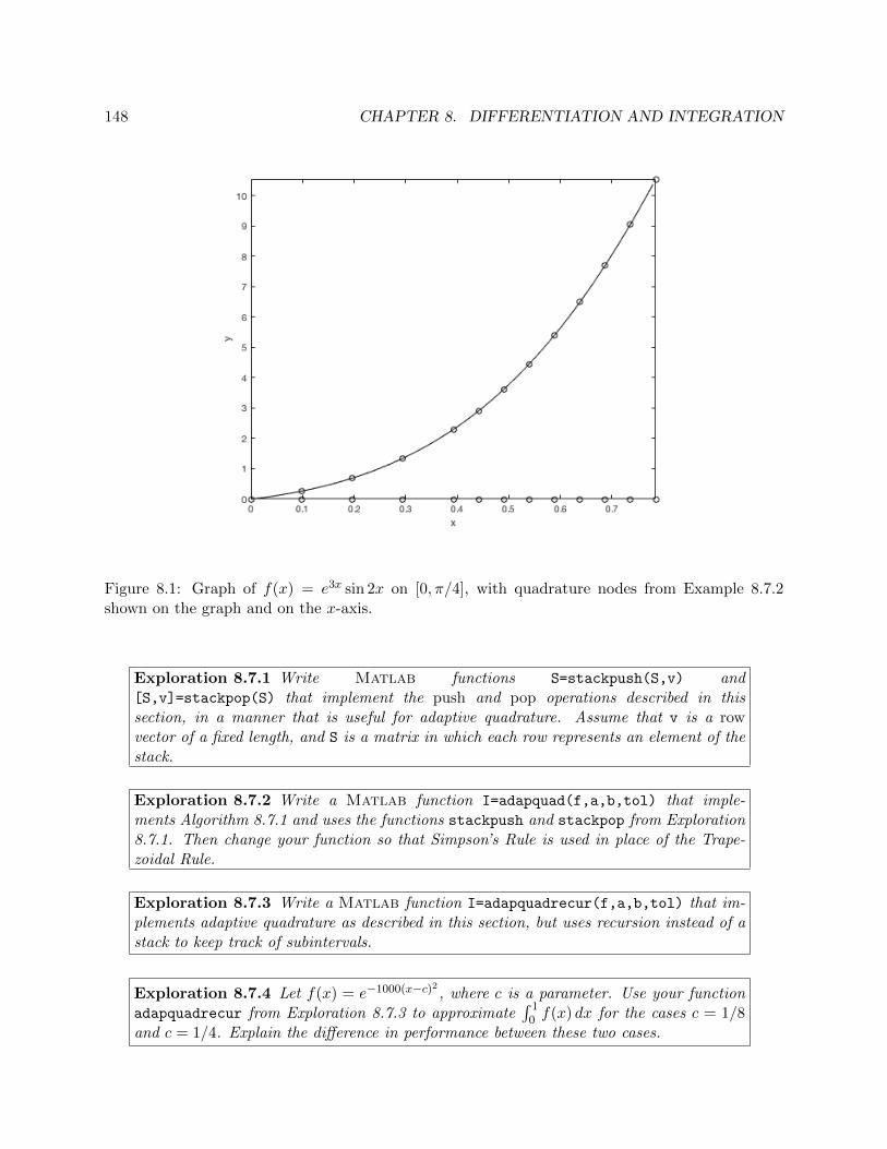
148 CHAPTER 8. DIFFERENTIATION AND INTEGRATION
Figure 8.1: Graph of f(x) = e3x sin 2x on [0, π/4], with quadrature nodes from Example 8.7.2shown on the graph and on the x-axis.
Exploration 8.7.1 Write Matlab functions S=stackpush(S,v) and[S,v]=stackpop(S) that implement the push and pop operations described in thissection, in a manner that is useful for adaptive quadrature. Assume that v is a rowvector of a fixed length, and S is a matrix in which each row represents an element of thestack.
Exploration 8.7.2 Write a Matlab function I=adapquad(f,a,b,tol) that imple-ments Algorithm 8.7.1 and uses the functions stackpush and stackpop from Exploration8.7.1. Then change your function so that Simpson’s Rule is used in place of the Trape-zoidal Rule.
Exploration 8.7.3 Write a Matlab function I=adapquadrecur(f,a,b,tol) that im-plements adaptive quadrature as described in this section, but uses recursion instead of astack to keep track of subintervals.
Exploration 8.7.4 Let f(x) = e−1000(x−c)2, where c is a parameter. Use your functionadapquadrecur from Exploration 8.7.3 to approximate
∫ 10 f(x) dx for the cases c = 1/8
and c = 1/4. Explain the difference in performance between these two cases.
8.8. MULTIPLE INTEGRALS 149
Exploration 8.7.5 Explain why a straightforward implementation of adaptive quadra-ture using recursion, as in your function adapquadrecur from Exploration 8.7.3, is notas efficient as it could be. What can be done to make it more efficient? Modify yourimplementation accordingly.
8.7.1 Concept Check
1. What is an automatic quadrature procedure?
2. What is the drawback of automatic quadrature?
3. What is adaptive quadrature?
4. How is the error estimated in adaptive quadrature?
5. What are the drawbacks of adaptive quadrature?
8.8 Multiple Integrals
As many problems in scientific computing involve two- or three-dimensional domains, it is essentialto be able to compute integrals over such domains. In this section, we explore the generalizationof techniques for integrals of functions of one variable to such multivariable cases.
8.8.1 Double Integrals
Double integrals can be evaluated using the following strategies:
• If a two-dimensional domain Ω can be decomposed into rectangles, then the integral of afunction f(x, y) over Ω can be computed by evaluating integrals of the form
I[f ] =
∫ b
a
∫ d
cf(x, y) dy dx. (8.23)
Then, to evaluate I[f ], one can use a Cartesian product rule, whose nodes and weights areobtained by combining one-dimensional quadrature rules that are applied to each dimension.For example, if functions of x are integrated along the line between x = a and x = b usingnodes xi and weights wi, for i = 1, . . . , n, and if functions of y are integrated along the linebetween y = c and y = d using nodes yi and weights zi, for i = 1, . . . ,m, then the resultingCartesian product rule
Qn,m[f ] =n∑i=1
m∑j=1
f(xi, yj)wizj
has nodes (xi, yj) and corresponding weights wizj for i = 1, . . . , n and j = 1, . . . ,m.
• If the domain Ω can be described as the region between two curves y1(x) and y2(x) forx ∈ [a, b], then we can write
I[f ] =
∫ ∫Ωf(x, y) dA
150 CHAPTER 8. DIFFERENTIATION AND INTEGRATION
as an iterated integral
I[f ] =
∫ b
a
∫ y2(x)
y1(x)f(x, y) dy dx
which can be evaluated by applying a one-dimensional quadrature rule to compute the outerintegral
I[f ] =
∫ b
ag(x) dx
where g(x) is evaluated by using a one-dimensional quadrature rule to compute the innerintegral
g(x) =
∫ y2(x)
y1(x)f(x, y) dy.
• For various simple regions such as triangles, there exist cubature rules that are not combi-nations of one-dimensional quadrature rules. Cubature rules are more direct generalizationsof quadrature rules, in that they evaluate the integrand at selected nodes and use weightsdetermined by the geometry of the domain and the placement of the nodes.
It should be noted that all of these strategies apply to certain special cases. The first algorithmcapable of integrating over a general two-dimensional domain was developed by Lambers and Rice[114]. This algorithm combines the second and third strategies described above, decomposing thedomain into subdomains that are either triangles or regions between two curves.
Example 8.8.1 We will use the Composite Trapezoidal Rule with m = n = 2 to evaluate thedouble integral ∫ 1/2
0
∫ 1/2
0ey−x dy dx.
The Composite Trapezoidal Rule with n = 2 subintervals is∫ b
af(x) dx ≈ h
2
[f(a) + 2f
(a+ b
2
)+ f(b)
], h =
b− an
.
If a = 0 and b = 1/2, then h = (1/2− 0)/2 = 1/4 and this simplifies to∫ 1/2
0f(x) dx ≈ 1
8[f(0) + 2f(1/4) + f(1/2)].
We first use this rule to evaluate the “single” integral∫ 1/2
0g(x) dx
where
g(x) =
∫ 1
0ey−x dy.
8.8. MULTIPLE INTEGRALS 151
This yields∫ 1/2
0
∫ 1/2
0ey−x dy dx =
∫ 1/2
0g(x) dx
≈ 1
8[g(0) + 2g(1/4) + g(1/2)]
≈ 1
8
[∫ 1/2
0ey−0 dy + 2
∫ 1/2
0ey−1/4 dy +
∫ 1/2
0ey−1/2 dy
].
Now, to evaluate each of these integrals, we use the Composite Trapezoidal Rule in the y-directionwith m = 2. If we let k denote the step size in the y-direction, we have k = (1/2− 0)/2 = 1/4, andtherefore we have∫ 1/2
0
∫ 1/2
0ey−x dy dx ≈ 1
8
[∫ 1/2
0ey−0 dy + 2
∫ 1/2
0ey−1/4 dy +
∫ 1/2
0ey−1/2 dy
]
≈ 1
8
[1
8
[e0−0 + 2e1/4−0 + e1/2−0
]+
21
8
[e0−1/4 + 2e1/4−1/4 + e1/2−1/4
]+
1
8
[e0−1/2 + 2e1/4−1/2 + e1/2−1/2
]]≈ 1
64
[e0 + 2e1/4 + e1/2
]+
1
32
[e−1/4 + 2e0 + e1/4
]+
1
64
[e−1/2 + 2e−1/4 + e0
]≈ 3
32e0 +
1
16e−1/4 +
1
64e−1/2 +
1
16e1/4 +
1
64e1/2
≈ 0.25791494889765.
The exact value, to 15 digits, is 0.255251930412762. The error is 2.66 × 10⁻³, which is to beexpected due to the use of few subintervals, and the fact that the Composite Trapezoidal Rule isonly second-order-accurate. 2
Example 8.8.2 We will use the Composite Simpson’s Rule with n = 2 and m = 4 to evaluate thedouble integral ∫ 1
0
∫ 2x
xx2 + y3 dy dx.
In this case, the domain of integration described by the limits is not a rectangle, but a triangledefined by the lines y = x, y = 2x, and x = 1. The Composite Simpson’s Rule with n = 2subintervals is ∫ b
af(x) dx ≈ h
3
[f(a) + 4f
(a+ b
2
)+ f(b)
], h =
b− an
.

152 CHAPTER 8. DIFFERENTIATION AND INTEGRATION
If a = 0 and b = 1, then h = (1− 0)/2 = 1/2, and this simplifies to∫ 1/2
0f(x) dx ≈ 1
6[f(0) + 4f(1/2) + f(1)].
We first use this rule to evaluate the “single” integral∫ 1
0g(x) dx
where
g(x) =
∫ 2x
xx2 + y3 dy.
This yields∫ 1
0
∫ 2x
xx2 + y3 dy dx =
∫ 1
0g(x) dx
≈ 1
6[g(0) + 4g(1/2) + g(1)]
≈ 1
6
[∫ 0
002 + y3 dy + 4
∫ 1
1/2
(1
2
)2
+ y3 dy +
∫ 2
112 + y3 dy
].
The first integral will be zero, since the limits of integration are equal. To evaluate the secondand third integrals, we use the Composite Simpson’s Rule in the y-direction with m = 4. If we letk denote the step size in the y-direction, we have k = (2x − x)/4 = x/4, and therefore we havek = 1/8 for the second integral and k = 1/4 for the third. This yields∫ 1
0
∫ 2x
xx2 + y3 dy dx ≈ 1
6
[4
∫ 1
1/2
(1
2
)2
+ y3 dy +
∫ 2
112 + y3 dy
]
≈ 1
6
4
1
24
[(1
4+
(1
2
)3)
+ 4
(1
4+
(5
8
)3)
+ 2
(1
4+
(3
4
)3)
+
4
(1
4+
(7
8
)3)
+
(1
4+ 13
)]+
1
12
[(1 + 13
)+ 4
(1 +
(5
4
)3)
+
2
(1 +
(3
2
)3)
+ 4
(1 +
(7
4
)3)
+(1 + 23
)]≈ 1.03125.
The exact value is 1. The error 3.125 × 10⁻² is rather large, which is to be expected due to thepoor distribution of nodes through the triangular domain of integration. A better distributionis achieved if we use n = 4 and m = 2, which yields the much more accurate approximation of1.001953125. 2
Exploration 8.8.1 Write a Matlab function I=quadcomptrap2d(f,a,b,c,d,m,n)
that approximates (8.23) using the Composite Trapezoidal Rule with m subintervals inthe x-direction and n subintervals in the y-direction.
8.8. MULTIPLE INTEGRALS 153
Exploration 8.8.2 Generalize your function quadcomptrap2d from Exploration 8.8.1 sothat the arguments c and d can be either scalars or function handles. If they are functionhandles, then your function approximates the integral
I[f ] =
∫ b
a
∫ d(x)
c(x)f(x, y) dy dx.
Hint: use the Matlab function isnumeric to determine whether c and d are numbers.
Exploration 8.8.3 Generalize your function quadcomptrap2d from Exploration 8.8.2so that the arguments a, b, c and d can be either scalars or function handles. If a and b
are function handles, then your function approximates the integral
I[f ] =
∫ d
c
∫ b(y)
a(y)f(x, y) dx dy.
Exploration 8.8.4 Use the error formula for the Composite Trapezoidal Rule to obtainan error formula for a Cartesian product rule such as the one implemented in Exploration8.8.1. As in that exploration, assume that m subintervals are used in the x-direction andn subintervals in the y-direction. Hint: first, apply the single-variable error formula tothe integral ∫ b
ag(x) dx, g(x) =
∫ d
cf(x, y) dy.
8.8.2 Higher Dimensions
The techniques presented in this section can readily be adapted for the purpose of approximatingtriple integrals. This adaptation is carried out in the following exercises.
Exploration 8.8.5 Write a Matlab function I=quadcomptrap3d(f,a,b,c,d,s,t,m,n,p)
that approximates ∫ b
a
∫ d
c
∫ t
sf(x, y, z) dz dy dx
using the Composite Trapezoidal Rule with m subintervals in the x-direction, n subin-tervals in the y-direction, and p subintervals in the z-direction. Hint: use your functionquadcomptrap2d from Exploration 8.8.1 to simplify the implementation.
Exploration 8.8.6 Modify your function quadcomptrap3d from Exploration 8.8.5 to ob-tain a function quadcompsimp3d that uses the Composite Simpson’s Rule in each direc-tion. Then, use an approach similar to that used in Exploration 8.8.4 to obtain an errorformula for the Cartesian product rule used in quadcompsimp3d.
154 CHAPTER 8. DIFFERENTIATION AND INTEGRATION
Exploration 8.8.7 Generalize your function quadcomptrap3d from Exploration 8.8.5so that any of the arguments a, b, c, d, s and t can be either scalars or function handles.For example, if a and b are scalars, c and d are function handles that have two inputarguments, and s and t are function handles that have one input argument, then yourfunction approximates the integral
I[f ] =
∫ b
a
∫ t(x)
s(x)
∫ d(x,z)
c(x,z)f(x, y, z) dy dz dx.
Hint: use the Matlab function isnumeric to determine whether any arguments arenumbers, and the function nargin to determine how many arguments a function handlerequires.
In more than three dimensions, generalizations of quadrature rules are not practical, sincethe number of function evaluations needed to attain sufficient accuracy grows very rapidly as thenumber of dimensions increases. An alternative is the Monte Carlo Method, which samples theintegrand at n randomly selected points and attempts to compute the mean value of the integrandon the entire domain. The method converges rather slowly but its convergence rate depends onlyon n, not the number of dimensions.
8.8.3 Concept Check
1. What is a Cartesian product rule?
2. How can a double integral be expressed as two single integrals?
3. What is a cubature rule? How does it differ from a Cartesian product rule?
4. What is problematic about generalization of quadrature rules to integrals over higher-dimensionaldomains?
5. What are Monte Carlo methods for integrals, and for what kinds of integrals are they used?
8.9 Additional Resources
Differentiation matrices are covered in greater detail by Trefethen in [185], in the context of spec-tral methods, which are introduced in Chapter ??. Beyond the scope of this text is automaticdifferentiation, also known as algorithmic differentiation. The main idea is to generate code forthe derivative of a function f by repeatedly applying the Chain Rule to produce statements thatrepresent the derivatives of the statements that implement f. This topic is covered in [84, 138].
The classic text by Davis and Rabinowitz [42] includes a wealth of knowledge about numericalintegration. In addition to expansion on the material presented in this chapter, their text also coverstopics beyond the scope of this book, such as Monte Carlo techniques and improper integrals, whichwere briefly alluded to in Section 8.5. Other general references on numerical integration include[58, 60, 113].
Tables of nodes and weights for Gauss quadrature rules can be found in [1, 181, 205]. Ex-trapolation techniques are covered extensively in [28, 104, 202]. A paper by Gander and Gautschi

8.10. EXERCISES 155
[71] provides an overview of adaptive quadrature, including the choice of termination criteria anddeficiencies in known adaptive quadrature routines. Further discussion of drawbacks of adaptivequadrature can be found in [126, 128]. An algorithm for approximating double integrals with 1-D adaptive quadrature routines is presented in [70]. General references on the approximation ofmultiple integrals are [36, 87, 127, 170, 180]. Monte Carlo methods in particular are covered in [91].
QUADPACK is a FORTRAN 77 library of routines for approximating one-dimensional integrals.As of this writing, the last stable release was thirty years ago, but its routines are still used insoftware packages such as Octave and R. QUADPACK is available at
http://nines.cs.kuleuven.be/software/QUADPACK
and its routines are documented in [150].
8.10 Exercises
1. Use Taylor series expansion to derive a finite difference approximation to f ′′′(x0) that usesthe points x0 ±m and x0 ± 2h. What is the error formula for this approximation?
2. Consider the general two-point approximation of the second derivative,
f ′′(x0) ≈ 2h1f(x0 − h2)− (h1 + h2)f(x0) + h2f(x0 + h1)
h1h2(h1 + h2).
(a) Prove that this approximation is equal to 2f [x0−h2, x0, x0 +h1], or 2 times the second-order divided difference (as in Section 6.3) of f over the points x0− h2, x0, and x0 + h1.
(b) Prove that this approximation is first-order accurate unless h1 = h2.
3. Let f(x) = sinx and x0 = 1.2. Consider the centered-difference approximation of f ′′(x0),
f ′′(x0) =f(x−1)− 2f(x0) + f(x1)
h2+O(h2),
where xi = x0 + ih, and the error formula is derived in Exploration 8.1.6. In this exercise,we account for roundoff error in this formula by replacing each expression of the form f(xi)with f(xi)(1 + εi), where we assume |εi| ≤ u with u being the machine precision.
(a) Show that the error in this approximation satisfies∣∣∣∣f ′′(x0)− f(x−1)− 2f(x0) + f(x1)
h2
∣∣∣∣ ≤ Mh2
12+
4u
h2,
where |f (4)(x)| ≤M on [x1, x2].
(b) Find the value of h that minimizes the error bound in part 3a.
(c) Use this approximation to approximate f ′′(x0), with h = 2−p for p = 0, 1, 2, . . . , 16. Plotthe errors against these values of h on a logarithmic scale (that is, use loglog). Estimatethe value of h at which the minimum error is achieved. How does this compare to theoptimal h found in part 3b? Use the value of the Matlab variable eps for u.
4. The following tabular data is used to describe a function f(x):
156 CHAPTER 8. DIFFERENTIATION AND INTEGRATION
x 0 1.5 2 3 4.5 5 6
f(x) 1 1.5 3 4 4.5 7 7.5
Use three-point finite-difference approximations to approximate f ′(x) at each of the x-valueslisted in the table. Note: it will be easiest to use interpolation rather than Taylor expansion.You may use polyfit to construct interpolating polynomials that fit the given data, rather
than deriving general finite-difference formulas. Do the results seem reasonable whencompared to a graph of f(x) based on this data?
5. Derive Simpson’s Rule by explicitly computing the weights using (8.9).
6. Let H3(x) be the Hermite interpolating polynomial of f(x) at x = a, b. Use this polynomialto derive the Corrected Trapezoidal Rule∫ b
af(x) dx ≈ b− a
2[f(a) + f(b)] +
(b− a)2
12[f ′(a)− f ′(b)] +
(b− a)5
720f (5)(ξ), ξ ∈ [a, b].
Include the derivation of the error formula in your answer. How does the accuracy of this rulecompare to Simpson’s Rule, when applied to I[f ] =
∫ 10 e
x dx? Hint: Use the Newton form ofH3(x).
7. (a) Compute the weights w1, w2, . . . , wn for closed Newton-Cotes rules with n = 4 and n = 5nodes on [−1, 1].
(b) Compare the weights from part 7a to the weights for the Trapezoidal Rule and Simpson’sRule on [−1, 1], which are also closed Newton-Cotes rules. What similarity do you notice?
(c) Prove that this property of the weights applies to a general interpolatory quadraturerule on [a, b].
8. Assume that f ′′(x) ≥ 0 on [a, b]. Let Mn[f ] be the approximation of I[f ] computed usingthe n-node Composite Midpoint Rule on [a, b], and similarly, let Tn[f ] be the approximationcomputed using the Composite Trapezoidal Rule. Prove that
Mn[f ] ≤ I[f ] ≤ Tn[f ].
9. Is it generally more accurate to apply a n-node Newton-Cotes rule Qn on each half of [a, b],or to apply a 2n-node Newton-Cotes rule Q2n to all of [a, b]? Explain your reasoning.
10. The gamma function Γ(z) is defined by
Γ(z) =
∫ ∞0
xz−1e−x dx.
It is worth noting that if z is a positive integer, then Γ(z) = (z − 1)! It can be evaluatedin Matlab using the gamma function. Use the following approaches to approximate Γ(z) forvarious values of z ∈ [1, 10]:
(a) Apply adaptive quadrature on a finite interval [0, b], where b is chosen so that∫∞b xz−1e−x
is negligibly small. Explain your approach to choosing b.
8.10. EXERCISES 157
(b) Use Gauss-Laguerre quadrature, which is Gauss quadrature with weight functionw(x) = e−x on the interval [0,∞). The nodes and weights can be looked up.
How do these approaches compare in terms of accuracy and efficiency?
11. Let pn denote the area of a n-sided regular polygon inscribed within the unit circle. Similarly,let qn denote the area of a n-sided regular polygon that circumscribes the unit circle. Then
pn = n sinπ
n, qn = n tan
π
n.
Since the area of the unit circle is π, pn and qn are both approximations of π that becomemore accurate as n increases.
(a) Let h = 1/n. Show that pn and qn satisfy
pn = π + a1h2 + a2h
4 + a3h6 + · · ·
qn = π + b1h2 + b2h
4 + b3h6 + · · ·
(b) Use Richardson Extrapolation to obtain O(h6)-accurate approximations of π from thevalues p4, p8, p16 and q4, q8, q16.
12. Use Richardson Extrapolation, applied to the centered difference formula for the secondderivative, to compute a 6th-order accurate approximation of f ′′(x0), where f(x) =
√x and
x0 = 1. Explain why Richardson extrapolation for this problem is much more effective thanit is when combined with the Composite Trapezoidal Rule to implement Romberg Integrationfor approximating I[f ] =
∫ 10
√x dx.
13. (a) Write a Matlab function y=piecewisef(x) that evaluates the piecewise function
f(x) =
ex x < 0e1−x x ≥ 0
and also plots the point (x, y) with a circle.
(b) Use your function adapquadrecur from Exploration 8.7.3 to approximate∫ 2−1 f(x) dx via
adaptive quadrature, with tolerance 10−3. By using piecewisef, the points at whichf(x) is evaluated will be displayed, as long as the command hold on is used first. Itis recommended that you plot the graph of f(x) on [−1, 2] first. What causes adaptivequadrature to be very inefficient in this case?
(c) How can you modify your function to address this inefficiency?
14. Let R = [−1, 1]× [−1, 1], and let (x0, y0) be a point outside of R. If there is a uniform chargedistribution within R, then the electrostatic potential at (x0, y0) given by
Φ(x0, y0) =
∫∫R
dx dy√(x− x0)2 + (y − y0)2
.
Use your function quadcomptrap from Exploration 8.8.1 to approximate this integral forpoints (x0, y0) chosen to be equally spaced points within the square R0 = [2, 10] × [2, 10].Then, use the Matlab function surf to plot the graph of Φ(x, y) on R0, which is a surface.Note: this will require storing the values of Φ(x0, y0) in a matrix.

158 CHAPTER 8. DIFFERENTIATION AND INTEGRATION

Part IV
Appendices
159

Appendix A
Review of Calculus
Among the mathematical problems that can be solved using techniques from numerical analysisare the basic problems of differential and integral calculus:
• computing the instantaneous rate of change of one quantity with respect to another, whichis a derivative, and
• computing the total change in a function over some portion of its domain, which is a definiteintegral.
Calculus also plays an essential role in the development and analysis of techniques used in numericalanalysis, including those techniques that are applied to problems not arising directly from calculus.Therefore, it is appropriate to review some basic concepts from calculus before we begin our studyof numerical analysis.
A.1 Limits and Continuity
A.1.1 Limits
The basic problems of differential and integral calculus described in the previous paragraph can besolved by computing a sequence of approximations to the desired quantity and then determiningwhat value, if any, the sequence of approximations approaches. This value is called a limit of thesequence. As a sequence is a function, we begin by defining, precisely, the concept of the limit of afunction.
161
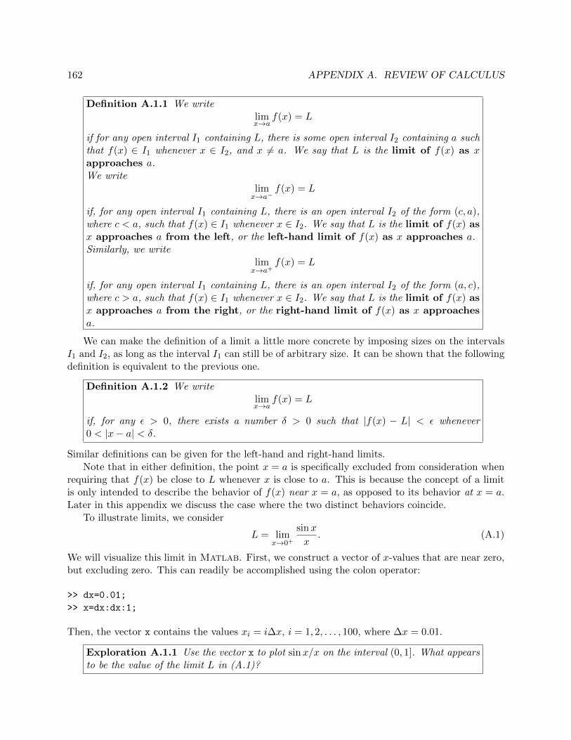
162 APPENDIX A. REVIEW OF CALCULUS
Definition A.1.1 We writelimx→a
f(x) = L
if for any open interval I1 containing L, there is some open interval I2 containing a suchthat f(x) ∈ I1 whenever x ∈ I2, and x 6= a. We say that L is the limit of f(x) as xapproaches a.We write
limx→a−
f(x) = L
if, for any open interval I1 containing L, there is an open interval I2 of the form (c, a),where c < a, such that f(x) ∈ I1 whenever x ∈ I2. We say that L is the limit of f(x) asx approaches a from the left, or the left-hand limit of f(x) as x approaches a.Similarly, we write
limx→a+
f(x) = L
if, for any open interval I1 containing L, there is an open interval I2 of the form (a, c),where c > a, such that f(x) ∈ I1 whenever x ∈ I2. We say that L is the limit of f(x) asx approaches a from the right, or the right-hand limit of f(x) as x approachesa.
We can make the definition of a limit a little more concrete by imposing sizes on the intervalsI1 and I2, as long as the interval I1 can still be of arbitrary size. It can be shown that the followingdefinition is equivalent to the previous one.
Definition A.1.2 We writelimx→a
f(x) = L
if, for any ε > 0, there exists a number δ > 0 such that |f(x) − L| < ε whenever0 < |x− a| < δ.
Similar definitions can be given for the left-hand and right-hand limits.
Note that in either definition, the point x = a is specifically excluded from consideration whenrequiring that f(x) be close to L whenever x is close to a. This is because the concept of a limitis only intended to describe the behavior of f(x) near x = a, as opposed to its behavior at x = a.Later in this appendix we discuss the case where the two distinct behaviors coincide.
To illustrate limits, we consider
L = limx→0+
sinx
x. (A.1)
We will visualize this limit in Matlab. First, we construct a vector of x-values that are near zero,but excluding zero. This can readily be accomplished using the colon operator:
>> dx=0.01;
>> x=dx:dx:1;
Then, the vector x contains the values xi = i∆x, i = 1, 2, . . . , 100, where ∆x = 0.01.
Exploration A.1.1 Use the vector x to plot sinx/x on the interval (0, 1]. What appearsto be the value of the limit L in (A.1)?

A.1. LIMITS AND CONTINUITY 163
The preceding exercise can be completed using a for loop, but it is much easier to use component-wise operators. Since x is a vector, the expression sin(x)/x would cause an error. Instead, the ./
operator can be used to perform componentwise division of the vectors sin(x) and x. The . canbe used with several other arithmetic operators to perform componentwise operations on matricesand vectors. For example, if A is a matrix, then A.^2 is a matrix in which each entry is the squareof the corresponding entry of A.
Exploration A.1.2 Use one statement to plot sinx/x on the interval (0, 1].
A.1.2 Limits of Functions of Several Variables
The notions of limit and continuity generalize to vector-valued functions and functions of severalvariables in a straightforward way.
Definition A.1.3 Given a function f : D ⊆ Rn → R and a point x0 ∈ D, we write
limx→x0
f(x) = L
if, for any ε > 0, there exists a δ > 0 such that
|f(x)− L| < ε
whenever x ∈ D and0 < ‖x− x0‖ < δ.
In this definition, we can use any appropriate vector norm ‖ · ‖, as discussed in Section B.12.
Definition A.1.4 We also say that f is continuous at a point x0 ∈ D if
limx→x0
f(x) = f(x0).
It can be shown f is continuous at x0 if its partial derivatives are bounded near x0.
Having defined limits and continuity for scalar-valued functions of several variables, we can nowdefine these concepts for vector-valued functions. Given a vector-valued function F : D ⊆ Rn → Rn,and x = (x1, x2, . . . , xn) ∈ D, we write
F(x) =
f1(x)f2(x)
...fn(x)
=
f1(x1, x2, . . . , xn)f2(x1, x2, . . . , xn)
...fn(x1, x2, . . . , xn)
where f1, f2, . . . , fn are the component functions, or coordinate functions, of F.
164 APPENDIX A. REVIEW OF CALCULUS
Definition A.1.5 Given F : D ⊆ Rn → Rn and x0 ∈ D, we say that
limx→x0
F(x) = L
if and only iflimx→x0
fi(x) = Li, i = 1, 2, . . . , n.
Similarly, we say that F is continuous at x0 if and only if each coordinate function fiis continuous at x0. Equivalently, F is continuous at x0 if
limx→x0
F(x) = F(x0).
A.1.3 Limits at Infinity
The concept of a limit defined above is useful for describing the behavior of a function f(x) as xapproaches a finite value a. However, suppose that the function f is a sequence, which is a functionthat maps N, the set of natural numbers, to R, the set of real numbers. We will denote such asequence by fn∞n=0, or simply fn. In numerical analysis, it is sometimes necessary to determinethe value that the terms of a sequence fn approach as n → ∞. Such a value, if it exists, is nota limit, as defined previously. However, it is natural to use the notation of limits to describe thisbehavior of a function. We therefore define what it means for a sequence fn to have a limit as nbecomes infinite.
Definition A.1.6 (Limit at Infinity) Let fn be a sequence defined for all integersnot less than some integer n0. We say that the limit of fn as n approaches ∞ isequal to L, and write
limn→∞
fn = L,
if for any open interval I containing L, there exists a number M such that fn ∈ I wheneverx > M .
Example A.1.7 Let the sequence fn∞n=1 be defined by fn = 1/n for every positive integer n.Then
limn→∞
fn = 0,
since for any ε > 0, no matter how small, we can find a positive integer n0 such that |fn| < ε forall n ≥ n0. In fact, for any given ε, we can choose n0 = d1/εe, where dxe, known as the ceilingfunction, denotes the smallest integer that is greater than or equal to x. 2
A.1.4 Continuity
In many cases, the limit of a function f(x) as x approached a could be obtained by simply computingf(a). Intuitively, this indicates that f has to have a graph that is one continuous curve, becauseany “break” or “jump” in the graph at x = a is caused by f approaching one value as x approachesa, only to actually assume a different value at a. This leads to the following precise definition ofwhat it means for a function to be continuous at a given point.
A.1. LIMITS AND CONTINUITY 165
Definition A.1.8 (Continuity) We say that a function f is continuous at a if
limx→a
f(x) = f(a).
We also say that f(x) has the Direct Substitution Property at x = a.We say that a function f is continuous from the right at a if
limx→a+
f(x) = f(a).
Similarly, we say that f is continuous from the left at a if
limx→a−
f(x) = f(a).
The preceding definition describes continuity at a single point. In describing where a functionis continuous, the concept of continuity over an interval is useful, so we define this concept as well.
Definition A.1.9 (Continuity on an Interval) We say that a function f is contin-uous on the interval (a, b) if f is continuous at every point in (a, b). Similarly, we saythat f is continuous on
1. [a, b) if f is continuous on (a, b), and continuous from the right at a.
2. (a, b] if f is continuous on (a, b), and continuous from the left at b.
3. [a, b] if f is continuous on (a, b), continuous from the right at a, and continuousfrom the left at b.
In numerical analysis, it is often necessary to construct a continuous function, such as a polyno-mial, based on data obtained by measurements and problem-dependent constraints. In this course,we will learn some of the most basic techniques for constructing such continuous functions by aprocess called interpolation.
A.1.5 The Intermediate Value Theorem
Suppose that a function f is continuous on some closed interval [a, b]. The graph of such a functionis a continuous curve connecting the points (a, f(a)) with (b, f(b)). If one were to draw such agraph, their pen would not leave the paper in the process, and therefore it would be impossibleto “avoid” any y-value between f(a) and f(b). This leads to the following statement about suchcontinuous functions.
Theorem A.1.10 (Intermediate Value Theorem) Let f be continuous on [a, b].Then, on (a, b), f assumes every value between f(a) and f(b); that is, for any valuey between f(a) and f(b), f(c) = y for some c in (a, b).
The Intermediate Value Theorem has a very important application in the problem of findingsolutions of a general equation of the form f(x) = 0, where x is the solution we wish to computeand f is a given continuous function. Often, methods for solving such an equation try to identifyan interval [a, b] where f(a) > 0 and f(b) < 0, or vice versa. In either case, the Intermediate Value
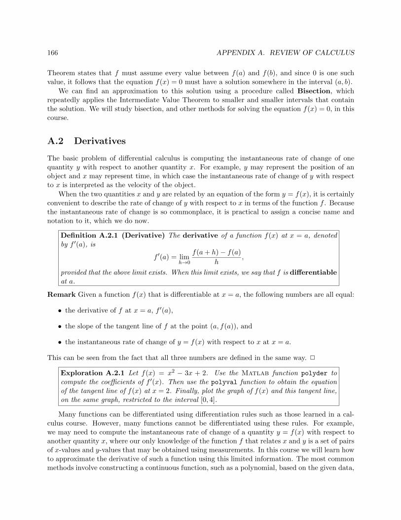
166 APPENDIX A. REVIEW OF CALCULUS
Theorem states that f must assume every value between f(a) and f(b), and since 0 is one suchvalue, it follows that the equation f(x) = 0 must have a solution somewhere in the interval (a, b).
We can find an approximation to this solution using a procedure called Bisection, whichrepeatedly applies the Intermediate Value Theorem to smaller and smaller intervals that containthe solution. We will study bisection, and other methods for solving the equation f(x) = 0, in thiscourse.
A.2 Derivatives
The basic problem of differential calculus is computing the instantaneous rate of change of onequantity y with respect to another quantity x. For example, y may represent the position of anobject and x may represent time, in which case the instantaneous rate of change of y with respectto x is interpreted as the velocity of the object.
When the two quantities x and y are related by an equation of the form y = f(x), it is certainlyconvenient to describe the rate of change of y with respect to x in terms of the function f . Becausethe instantaneous rate of change is so commonplace, it is practical to assign a concise name andnotation to it, which we do now.
Definition A.2.1 (Derivative) The derivative of a function f(x) at x = a, denotedby f ′(a), is
f ′(a) = limh→0
f(a+ h)− f(a)
h,
provided that the above limit exists. When this limit exists, we say that f is differentiableat a.
Remark Given a function f(x) that is differentiable at x = a, the following numbers are all equal:
• the derivative of f at x = a, f ′(a),
• the slope of the tangent line of f at the point (a, f(a)), and
• the instantaneous rate of change of y = f(x) with respect to x at x = a.
This can be seen from the fact that all three numbers are defined in the same way. 2
Exploration A.2.1 Let f(x) = x2 − 3x + 2. Use the Matlab function polyder tocompute the coefficients of f ′(x). Then use the polyval function to obtain the equationof the tangent line of f(x) at x = 2. Finally, plot the graph of f(x) and this tangent line,on the same graph, restricted to the interval [0, 4].
Many functions can be differentiated using differentiation rules such as those learned in a cal-culus course. However, many functions cannot be differentiated using these rules. For example,we may need to compute the instantaneous rate of change of a quantity y = f(x) with respect toanother quantity x, where our only knowledge of the function f that relates x and y is a set of pairsof x-values and y-values that may be obtained using measurements. In this course we will learn howto approximate the derivative of such a function using this limited information. The most commonmethods involve constructing a continuous function, such as a polynomial, based on the given data,
A.3. EXTREME VALUES 167
using interpolation. The polynomial can then be differentiated using differentiation rules. Since thepolynomial is an approximation to the function f(x), its derivative is an approximation to f ′(x).
A.2.1 Differentiability and Continuity
Consider a tangent line of a function f at a point (a, f(a)). When we consider that this tangentline is the limit of secant lines that can cross the graph of f at points on either side of a, it seemsimpossible that f can fail to be continuous at a. The following result confirms this: a functionthat is differentiable at a given point (and therefore has a tangent line at that point) must also becontinuous at that point.
Theorem A.2.2 If f is differentiable at a, then f is continuous at a.
It is important to keep in mind, however, that the converse of the above statement, “if fis continuous, then f is differentiable”, is not true. It is actually very easy to find examples offunctions that are continuous at a point, but fail to be differentiable at that point. As an extremeexample, it is known that there is a function that is continuous everywhere, but is differentiablenowhere.
Example A.2.3 The functions f(x) = |x| and g(x) = x1/3 are examples of functions that arecontinuous for all x, but are not differentiable at x = 0. The graph of the absolute value function|x| has a sharp corner at x = 0, since the one-sided limits
limh→0−
f(h)− f(0)
h= −1, lim
h→0+
f(h)− f(0)
h= 1
do not agree, but in general these limits must agree in order for f(x) to have a derivative at x = 0.
The cube root function g(x) = x1/3 is not differentiable at x = 0 because the tangent line tothe graph at the point (0, 0) is vertical, so it has no finite slope. We can also see that the derivativedoes not exist at this point by noting that the function g′(x) = (1/3)x−2/3 has a vertical asymptoteat x = 0. 2
Exploration A.2.2 Plot both of the functions from the preceding example on the interval[−1, 1]. Use the colon operator to create a vector of x-values and use the dot for performingcomponentwise operations on a vector, where applicable. From the plot, identify the non-differentiability in these continuous functions.
A.3 Extreme Values
In many applications, it is necessary to determine where a given function attains its minimum ormaximum value. For example, a business wishes to maximize profit, so it can construct a functionthat relates its profit to variables such as payroll or maintenance costs. We now consider the basicproblem of finding a maximum or minimum value of a general function f(x) that depends on asingle independent variable x. First, we must precisely define what it means for a function to havea maximum or minimum value.
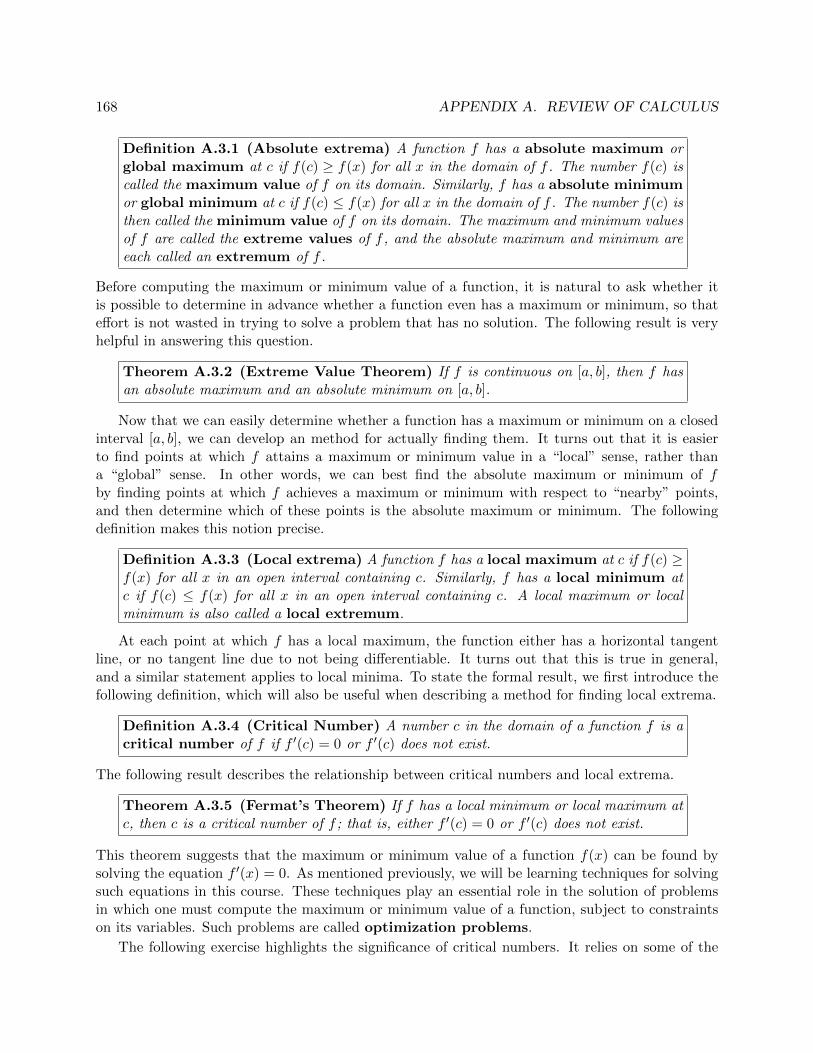
168 APPENDIX A. REVIEW OF CALCULUS
Definition A.3.1 (Absolute extrema) A function f has a absolute maximum orglobal maximum at c if f(c) ≥ f(x) for all x in the domain of f . The number f(c) iscalled the maximum value of f on its domain. Similarly, f has a absolute minimumor global minimum at c if f(c) ≤ f(x) for all x in the domain of f . The number f(c) isthen called the minimum value of f on its domain. The maximum and minimum valuesof f are called the extreme values of f , and the absolute maximum and minimum areeach called an extremum of f .
Before computing the maximum or minimum value of a function, it is natural to ask whether itis possible to determine in advance whether a function even has a maximum or minimum, so thateffort is not wasted in trying to solve a problem that has no solution. The following result is veryhelpful in answering this question.
Theorem A.3.2 (Extreme Value Theorem) If f is continuous on [a, b], then f hasan absolute maximum and an absolute minimum on [a, b].
Now that we can easily determine whether a function has a maximum or minimum on a closedinterval [a, b], we can develop an method for actually finding them. It turns out that it is easierto find points at which f attains a maximum or minimum value in a “local” sense, rather thana “global” sense. In other words, we can best find the absolute maximum or minimum of fby finding points at which f achieves a maximum or minimum with respect to “nearby” points,and then determine which of these points is the absolute maximum or minimum. The followingdefinition makes this notion precise.
Definition A.3.3 (Local extrema) A function f has a local maximum at c if f(c) ≥f(x) for all x in an open interval containing c. Similarly, f has a local minimum atc if f(c) ≤ f(x) for all x in an open interval containing c. A local maximum or localminimum is also called a local extremum.
At each point at which f has a local maximum, the function either has a horizontal tangentline, or no tangent line due to not being differentiable. It turns out that this is true in general,and a similar statement applies to local minima. To state the formal result, we first introduce thefollowing definition, which will also be useful when describing a method for finding local extrema.
Definition A.3.4 (Critical Number) A number c in the domain of a function f is acritical number of f if f ′(c) = 0 or f ′(c) does not exist.
The following result describes the relationship between critical numbers and local extrema.
Theorem A.3.5 (Fermat’s Theorem) If f has a local minimum or local maximum atc, then c is a critical number of f ; that is, either f ′(c) = 0 or f ′(c) does not exist.
This theorem suggests that the maximum or minimum value of a function f(x) can be found bysolving the equation f ′(x) = 0. As mentioned previously, we will be learning techniques for solvingsuch equations in this course. These techniques play an essential role in the solution of problemsin which one must compute the maximum or minimum value of a function, subject to constraintson its variables. Such problems are called optimization problems.
The following exercise highlights the significance of critical numbers. It relies on some of the

A.4. INTEGRALS 169
Matlab functions for working with polynomials that were introduced in Section 1.2.
Exploration A.3.1 Consider the polynomial f(x) = x3−4x2 +5x−2. Plot the graph ofthis function on the interval [0, 3]. Use the colon operator to create a vector of x-valuesand use the dot for componentwise operations on vectors wherever needed. Then, use thepolyder and roots functions to compute the critical numbers of f(x). How do they relateto the absolute maximum and minimum values of f(x) on [0, 3], or any local maxima orminima on this interval?
A.4 Integrals
There are many cases in which some quantity is defined to be the product of two other quantities.For example, a rectangle of width w has uniform height h, and the area A of the rectangle is givenby the formula A = wh. Unfortunately, in many applications, we cannot necessarily assume thatcertain quantities such as height are constant, and therefore formulas such as A = wh cannot beused directly. However, they can be used indirectly to solve more general problems by employingthe notation known as integral calculus.
Suppose we wish to compute the area of a shape that is not a rectangle. To simplify thediscussion, we assume that the shape is bounded by the vertical lines x = a and x = b, the x-axis,and the curve defined by some continuous function y = f(x), where f(x) ≥ 0 for a ≤ x ≤ b. Then,we can approximate this shape by n rectangles that have width ∆x = (b− a)/n and height f(xi),where xi = a+ i∆x, for i = 0, . . . , n. We obtain the approximation
A ≈ An =n∑i=1
f(xi)∆x.
Intuitively, we can conclude that as n → ∞, the approximate area An will converge to the exactarea of the given region. This can be seen by observing that as n increases, the n rectangles definedabove comprise a more accurate approximation of the region.
More generally, suppose that for each n = 1, 2, . . ., we define the quantity Rn by choosing pointsa = x0 < x1 < · · · < xn = b, and computing the sum
Rn =n∑i=1
f(x∗i )∆xi, ∆xi = xi − xi−1, xi−1 ≤ x∗i ≤ xi.
The sum that defines Rn is known as a Riemann sum. Note that the interval [a, b] need notbe divided into subintervals of equal width, and that f(x) can be evaluated at arbitrary pointsbelonging to each subinterval.
If f(x) ≥ 0 on [a, b], then Rn converges to the area under the curve y = f(x) as n → ∞,provided that the widths of all of the subintervals [xi−1, xi], for i = 1, . . . , n, approach zero. Thisbehavior is ensured if we require that
limn→∞
δ(n) = 0, where δ(n) = max1≤i≤n
∆xi.
This condition is necessary because if it does not hold, then, as n→∞, the region formed by then rectangles will not converge to the region whose area we wish to compute. If f assumes negative
170 APPENDIX A. REVIEW OF CALCULUS
values on [a, b], then, under the same conditions on the widths of the subintervals, Rn convergesto the net area between the graph of f and the x-axis, where area below the x-axis is countednegatively.
Definition A.4.1 We define the definite integral of f(x) from a to b by∫ b
af(x) dx = lim
n→∞Rn,
where the sequence of Riemann sums Rn∞n=1 is defined so that δ(n) → 0 as n → ∞,as in the previous discussion. The function f(x) is called the integrand, and the valuesa and b are the lower and upper limits of integration, respectively. The process ofcomputing an integral is called integration.
In Chapter 8, we will study the problem of computing an approximation to the definite integralof a given function f(x) over an interval [a, b]. We will learn a number of techniques for computingsuch an approximation, and all of these techniques involve the computation of an appropriateRiemann sum.
Exploration A.4.1 Let f(x) = e−x2. Write a Matlab function that takes as input a
parameter n, and computes the Riemann sum Rn for f(x) using n rectangles. Use a for
loop to compute the Riemann sum. First use x∗i = xi−1, then use x∗i = xi, and then usex∗i = (xi−1 + xi)2. For each case, compute Riemann sums for several values of n. Whatcan you observe about the convergence of the Riemann sum in these three cases?
A.5 The Mean Value Theorem
While the derivative describes the behavior of a function at a point, we often need to understandhow the derivative influences a function’s behavior on an interval. This understanding is essentialin numerical analysis because, it is often necessary to approximate a function f(x) by a functiong(x) using knowledge of f(x) and its derivatives at various points. It is therefore natural to askhow well g(x) approximates f(x) away from these points.
The following result, a consequence of Fermat’s Theorem, gives limited insight into the rela-tionship between the behavior of a function on an interval and the value of its derivative at apoint.
Theorem A.5.1 (Rolle’s Theorem) If f is continuous on a closed interval [a, b] andis differentiable on the open interval (a, b), and if f(a) = f(b), then f ′(c) = 0 for somenumber c in (a, b).
By applying Rolle’s Theorem to a function f , then to its derivative f ′, its second derivative f ′′, andso on, we obtain the following more general result, which will be useful in analyzing the accuracyof methods for approximating functions by polynomials.
Theorem A.5.2 (Generalized Rolle’s Theorem) Let x0, x1, x2, . . ., xn be distinctpoints in an interval [a, b]. If f is n times differentiable on (a, b), and if f(xi) = 0 fori = 0, 1, 2, . . . , n, then f (n)(c) = 0 for some number c in (a, b).
A.5. THE MEAN VALUE THEOREM 171
A more fundamental consequence of Rolle’s Theorem is the Mean Value Theorem itself, whichwe now state.
Theorem A.5.3 (Mean Value Theorem) If f is continuous on a closed interval [a, b]and is differentiable on the open interval (a, b), then
f(b)− f(a)
b− a= f ′(c)
for some number c in (a, b).
Remark The expression
f(b)− f(a)
b− a
is the slope of the secant line passing through the points (a, f(a)) and (b, f(b)). The Mean ValueTheorem therefore states that under the given assumptions, the slope of this secant line is equal tothe slope of the tangent line of f at the point (c, f(c)), where c ∈ (a, b). 2
The Mean Value Theorem has the following practical interpretation: the average rate of change ofy = f(x) with respect to x on an interval [a, b] is equal to the instantaneous rate of change y withrespect to x at some point in (a, b).
A.5.1 The Mean Value Theorem for Integrals
Suppose that f(x) is a continuous function on an interval [a, b]. Then, by the Fundamental Theoremof Calculus, f(x) has an antiderivative F (x) defined on [a, b] such that F ′(x) = f(x). If we applythe Mean Value Theorem to F (x), we obtain the following relationship between the integral of fover [a, b] and the value of f at a point in (a, b).
Theorem A.5.4 (Mean Value Theorem for Integrals) If f is continuous on [a, b],then ∫ b
af(x) dx = f(c)(b− a)
for some c in (a, b).
In other words, f assumes its average value over [a, b], defined by
fave =1
b− a
∫ b
af(x) dx,
at some point in [a, b], just as the Mean Value Theorem states that the derivative of a functionassumes its average value over an interval at some point in the interval.
The Mean Value Theorem for Integrals is also a special case of the following more general result.
172 APPENDIX A. REVIEW OF CALCULUS
Theorem A.5.5 (Weighted Mean Value Theorem for Integrals) If f is continuouson [a, b], and g is a function that is integrable on [a, b] and does not change sign on [a, b],then ∫ b
af(x)g(x) dx = f(c)
∫ b
ag(x) dx
for some c in (a, b).
In the case where g(x) is a function that is easy to antidifferentiate and f(x) is not, this theoremcan be used to obtain an estimate of the integral of f(x)g(x) over an interval.
Example A.5.6 Let f(x) be continuous on the interval [a, b]. Then, for any x ∈ [a, b], by theWeighted Mean Value Theorem for Integrals, we have∫ x
af(s)(s− a) ds = f(c)
∫ x
a(s− a) ds = f(c)
(s− a)2
2
∣∣∣∣xa
= f(c)(x− a)2
2,
where a < c < x. It is important to note that we can apply the Weighted Mean Value Theorembecause the function g(x) = (x− a) does not change sign on [a, b]. 2
A.6 Taylor’s Theorem
In many cases, it is useful to approximate a given function f(x) by a polynomial, because one canwork much more easily with polynomials than with other types of functions. As such, it is necessaryto have some insight into the accuracy of such an approximation. The following theorem, which isa consequence of the Weighted Mean Value Theorem for Integrals, provides this insight.
Theorem A.6.1 (Taylor’s Theorem) Let f be n times continuously differentiable onan interval [a, b], and suppose that f (n+1) exists on [a, b]. Let x0 ∈ [a, b]. Then, for anypoint x ∈ [a, b],
f(x) = Pn(x) +Rn(x),
where
Pn(x) =
n∑j=0
f (j)(x0)
j!(x− x0)j
= f(x0) + f ′(x0)(x− x0) +1
2f ′′(x0)(x− x0)2 + · · ·+ f (n)(x0)
n!(x− x0)n
and
Rn(x) =
∫ x
x0
f (n+1)(s)
n!(x− s)n ds =
f (n+1)(ξ(x))
(n+ 1)!(x− x0)n+1,
where ξ(x) is between x0 and x.
The polynomial Pn(x) is the nth Taylor polynomial of f with center x0, and the expression Rn(x)is called the Taylor remainder of Pn(x). When the center x0 is zero, the nth Taylor polynomialis also known as the nth Maclaurin polynomial.
A.6. TAYLOR’S THEOREM 173
Exploration A.6.1 Plot the graph of f(x) = cosx on the interval [0, π], and then usethe hold command to include the graphs of P0(x), P2(x), and P4(x), the Maclaurinpolynomials of degree 0, 2 and 4, respectively, on the same plot but with different colorsand line styles. To what extent do these Taylor polynomials agree with f(x)?
The final form of the remainder is obtained by applying the Mean Value Theorem for Integralsto the integral form. As Pn(x) can be used to approximate f(x), the remainder Rn(x) is alsoreferred to as the truncation error of Pn(x). The accuracy of the approximation on an interval canbe analyzed by using techniques for finding the extreme values of functions to bound the (n+ 1)stderivative on the interval.
Because approximation of functions by polynomials is employed in the development and analysisof many techniques in numerical analysis, the usefulness of Taylor’s Theorem cannot be overstated.In fact, it can be said that Taylor’s Theorem is the Fundamental Theorem of Numerical Analysis,just as the theorem describing inverse relationship between derivatives and integrals is called theFundamental Theorem of Calculus.
The following examples illustrate how the nth-degree Taylor polynomial Pn(x) and the remain-der Rn(x) can be computed for a given function f(x).
Example A.6.2 If we set n = 1 in Taylor’s Theorem, then we have
f(x) = P1(x) +R1(x)
where
P1(x) = f(x0) + f ′(x0)(x− x0).
This polynomial is a linear function that describes the tangent line to the graph of f at the point(x0, f(x0)).
If we set n = 0 in the theorem, then we obtain
f(x) = P0(x) +R0(x),
where
P0(x) = f(x0)
and
R0(x) = f ′(ξ(x))(x− x0),
where ξ(x) lies between x0 and x. If we use the integral form of the remainder,
Rn(x) =
∫ x
x0
f (n+1)(s)
n!(x− s)n ds,
then we have
f(x) = f(x0) +
∫ x
x0
f ′(s) ds,
which is equivalent to the Total Change Theorem and part of the Fundamental Theorem of Calculus.Using the Mean Value Theorem for integrals, we can see how the first form of the remainder canbe obtained from the integral form. 2
174 APPENDIX A. REVIEW OF CALCULUS
Example A.6.3 Let f(x) = sinx. Then
f(x) = P3(x) +R3(x),
where
P3(x) = x− x3
3!= x− x3
6,
and
R3(x) =1
4!x4 sin ξ(x) =
1
24x4 sin ξ(x),
where ξ(x) is between 0 and x. The polynomial P3(x) is the 3rd Maclaurin polynomial of sinx, orthe 3rd Taylor polynomial with center x0 = 0.
If x ∈ [−1, 1], then
|Rn(x)| =∣∣∣∣ 1
24x4 sin ξ(x)
∣∣∣∣ =
∣∣∣∣ 1
24
∣∣∣∣ |x4|| sin ξ(x)| ≤ 1
24,
since | sinx| ≤ 1 for all x. This bound on |Rn(x)| serves as an upper bound for the error in theapproximation of sinx by P3(x) for x ∈ [−1, 1]. 2
Exploration A.6.2 On the interval [−1, 1], plot f(x) = sinx and its Taylor polynomialof degree 3 centered at x0 = 0, P3(x). How do they compare? In a separate figurewindow, plot the error R3(x) = f(x)− P3(x) on [−1, 1], and also plot the lines y = ± 1
24 ,corresponding to the upper bound on |R3(x)| from the preceding example. Confirm thatthe error actually does satisfy this bound.
Example A.6.4 Let f(x) = ex. Then
f(x) = P2(x) +R2(x),
where
P2(x) = 1 + x+x2
2,
and
R2(x) =x3
6eξ(x),
where ξ(x) is between 0 and x. The polynomial P2(x) is the 2nd Maclaurin polynomial of ex, orthe 2nd Taylor polynomial with center x0 = 0.
If x > 0, then R2(x) can become quite large, whereas its magnitude is much smaller if x < 0.Therefore, one method of computing ex using a Maclaurin polynomial is to use the nth Maclaurinpolynomial Pn(x) of ex when x < 0, where n is chosen sufficiently large so that Rn(x) is small forthe given value of x. If x > 0, then we instead compute e−x using the nth Maclaurin polynomialfor e−x, which is given by
Pn(x) = 1− x+x2
2− x3
6+ · · ·+ (−1)nxn
n!,
and then obtaining an approximation to ex by taking the reciprocal of our computed value of e−x.2
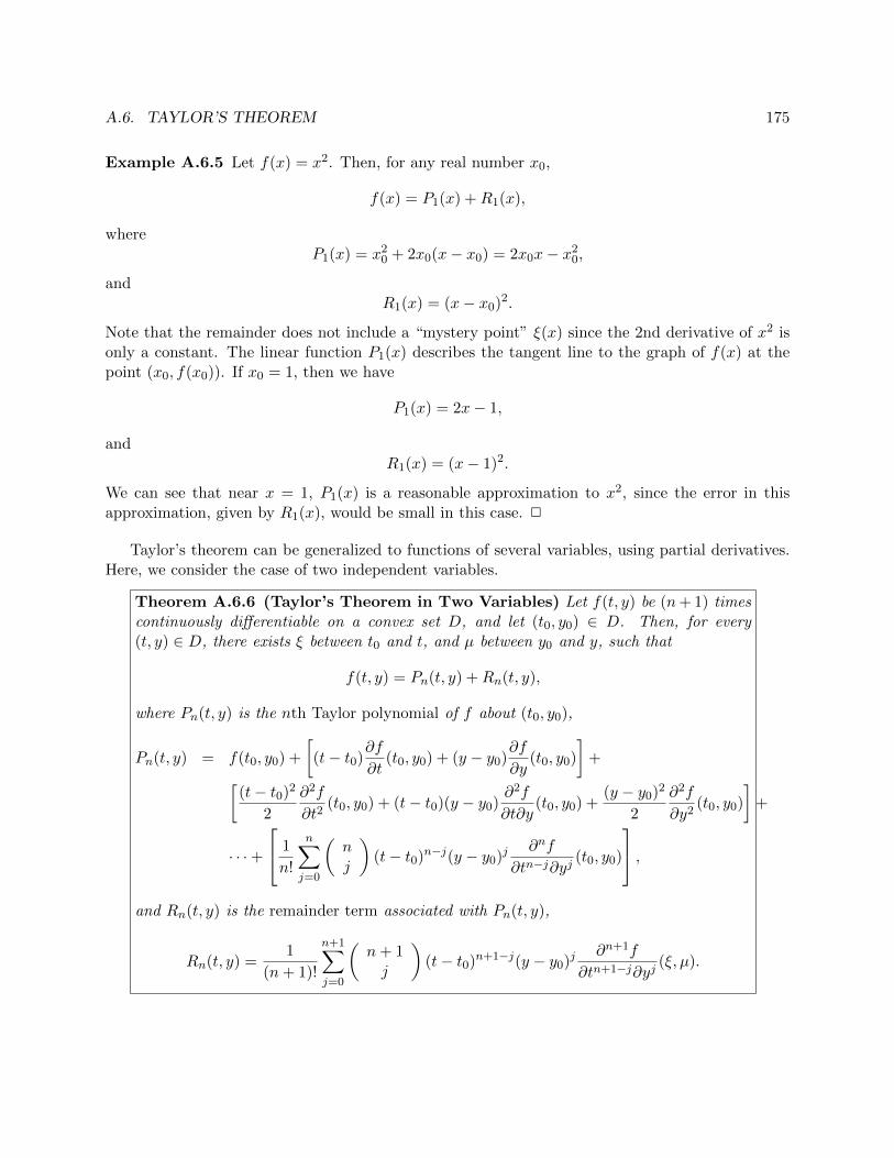
A.6. TAYLOR’S THEOREM 175
Example A.6.5 Let f(x) = x2. Then, for any real number x0,
f(x) = P1(x) +R1(x),
whereP1(x) = x2
0 + 2x0(x− x0) = 2x0x− x20,
andR1(x) = (x− x0)2.
Note that the remainder does not include a “mystery point” ξ(x) since the 2nd derivative of x2 isonly a constant. The linear function P1(x) describes the tangent line to the graph of f(x) at thepoint (x0, f(x0)). If x0 = 1, then we have
P1(x) = 2x− 1,
andR1(x) = (x− 1)2.
We can see that near x = 1, P1(x) is a reasonable approximation to x2, since the error in thisapproximation, given by R1(x), would be small in this case. 2
Taylor’s theorem can be generalized to functions of several variables, using partial derivatives.Here, we consider the case of two independent variables.
Theorem A.6.6 (Taylor’s Theorem in Two Variables) Let f(t, y) be (n+ 1) timescontinuously differentiable on a convex set D, and let (t0, y0) ∈ D. Then, for every(t, y) ∈ D, there exists ξ between t0 and t, and µ between y0 and y, such that
f(t, y) = Pn(t, y) +Rn(t, y),
where Pn(t, y) is the nth Taylor polynomial of f about (t0, y0),
Pn(t, y) = f(t0, y0) +
[(t− t0)
∂f
∂t(t0, y0) + (y − y0)
∂f
∂y(t0, y0)
]+[
(t− t0)2
2
∂2f
∂t2(t0, y0) + (t− t0)(y − y0)
∂2f
∂t∂y(t0, y0) +
(y − y0)2
2
∂2f
∂y2(t0, y0)
]+
· · ·+
1
n!
n∑j=0
(nj
)(t− t0)n−j(y − y0)j
∂nf
∂tn−j∂yj(t0, y0)
,and Rn(t, y) is the remainder term associated with Pn(t, y),
Rn(t, y) =1
(n+ 1)!
n+1∑j=0
(n+ 1j
)(t− t0)n+1−j(y − y0)j
∂n+1f
∂tn+1−j∂yj(ξ, µ).

176 APPENDIX A. REVIEW OF CALCULUS
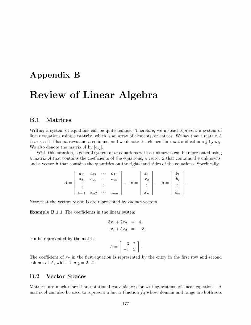
Appendix B
Review of Linear Algebra
B.1 Matrices
Writing a system of equations can be quite tedious. Therefore, we instead represent a system oflinear equations using a matrix, which is an array of elements, or entries. We say that a matrix Ais m× n if it has m rows and n columns, and we denote the element in row i and column j by aij .We also denote the matrix A by [aij ].
With this notation, a general system of m equations with n unknowns can be represented usinga matrix A that contains the coefficients of the equations, a vector x that contains the unknowns,and a vector b that contains the quantities on the right-hand sides of the equations. Specifically,
A =
a11 a12 · · · a1n
a21 a22 · · · a2n...
...am1 am2 · · · amn
, x =
x1
x2...xn
, b =
b1b2...bm
.Note that the vectors x and b are represented by column vectors.
Example B.1.1 The coefficients in the linear system
3x1 + 2x2 = 4,
−x1 + 5x2 = −3
can be represented by the matrix
A =
[3 2−1 5
].
The coefficient of x2 in the first equation is represented by the entry in the first row and secondcolumn of A, which is a12 = 2. 2
B.2 Vector Spaces
Matrices are much more than notational conveniences for writing systems of linear equations. Amatrix A can also be used to represent a linear function fA whose domain and range are both sets
177

178 APPENDIX B. REVIEW OF LINEAR ALGEBRA
of vectors called vector spaces. A vector space over a field (such as the field of real or complexnumbers) is a set of vectors, together with two operations: addition of vectors, and multiplicationof a vector by a scalar from the field.
Specifically, if u and v are vectors belonging to a vector space V over a field F , then the sumof u and v, denoted by u + v, is a vector in V , and the scalar product of u with a scalar α in F ,denoted by αu, is also a vector in V . These operations have the following properties:
• Commutativity: For any vectors u and v in V ,
u + v = v + u
• Associativity: For any vectors u, v and w in V ,
(u + v) + w = u + (v + w)
• Identity element for vector addition: There is a vector 0, known as the zero vector, such thatfor any vector u in V ,
u + 0 = 0 + u = u
• Additive inverse: For any vector u in V , there is a unique vector −u in V such that
u + (−u) = −u + u = 0
• Distributivity over vector addition: For any vectors u and v in V , and scalar α in F ,
α(u + v) = αu + αv
• Distributivity over scalar multiplication: For any vector u in V , and scalars α and β in F ,
(α+ β)u = αu + βu
• Associativity of scalar multiplication: For any vector u in V and any scalars α and β in F ,
α(βu) = (αβ)u
• Identity element for scalar multiplication: For any vector u in V ,
1u = u
Example B.2.1 Let V be the vector space R3. The vector addition operation on V consists ofadding corresponding components of vectors, as in 3
01
+
−245
=
146
.The scalar multiplication operation consists of scaling each component of a vector by a scalar:
1
2
301
=
32012
.2
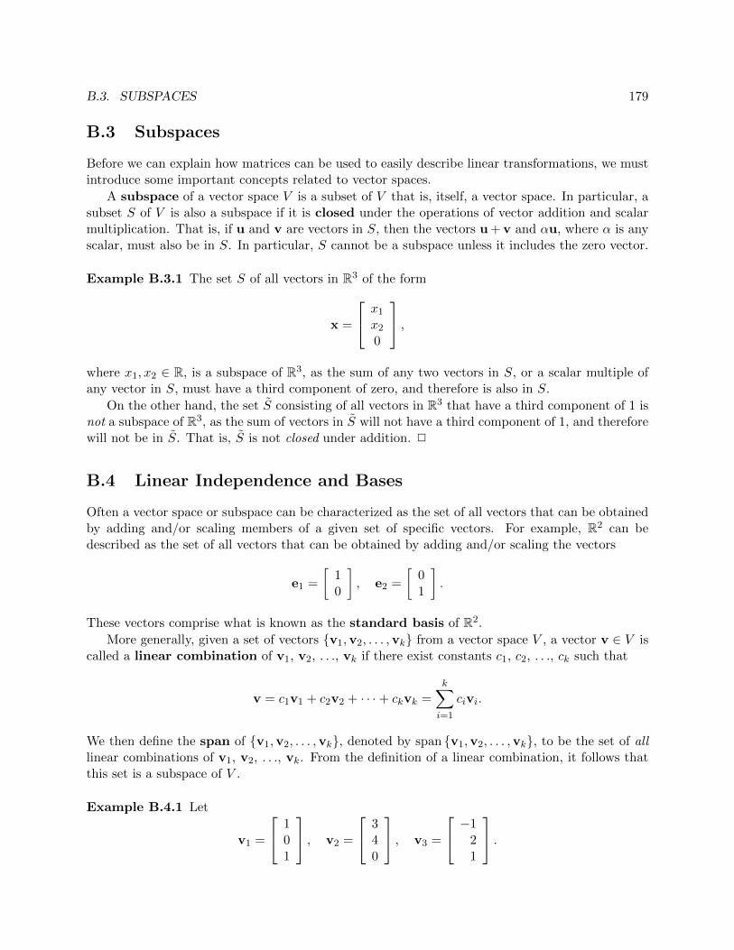
B.3. SUBSPACES 179
B.3 Subspaces
Before we can explain how matrices can be used to easily describe linear transformations, we mustintroduce some important concepts related to vector spaces.
A subspace of a vector space V is a subset of V that is, itself, a vector space. In particular, asubset S of V is also a subspace if it is closed under the operations of vector addition and scalarmultiplication. That is, if u and v are vectors in S, then the vectors u + v and αu, where α is anyscalar, must also be in S. In particular, S cannot be a subspace unless it includes the zero vector.
Example B.3.1 The set S of all vectors in R3 of the form
x =
x1
x2
0
,where x1, x2 ∈ R, is a subspace of R3, as the sum of any two vectors in S, or a scalar multiple ofany vector in S, must have a third component of zero, and therefore is also in S.
On the other hand, the set S consisting of all vectors in R3 that have a third component of 1 isnot a subspace of R3, as the sum of vectors in S will not have a third component of 1, and thereforewill not be in S. That is, S is not closed under addition. 2
B.4 Linear Independence and Bases
Often a vector space or subspace can be characterized as the set of all vectors that can be obtainedby adding and/or scaling members of a given set of specific vectors. For example, R2 can bedescribed as the set of all vectors that can be obtained by adding and/or scaling the vectors
e1 =
[10
], e2 =
[01
].
These vectors comprise what is known as the standard basis of R2.
More generally, given a set of vectors v1,v2, . . . ,vk from a vector space V , a vector v ∈ V iscalled a linear combination of v1, v2, . . ., vk if there exist constants c1, c2, . . ., ck such that
v = c1v1 + c2v2 + · · ·+ ckvk =
k∑i=1
civi.
We then define the span of v1,v2, . . . ,vk, denoted by span v1,v2, . . . ,vk, to be the set of alllinear combinations of v1, v2, . . ., vk. From the definition of a linear combination, it follows thatthis set is a subspace of V .
Example B.4.1 Let
v1 =
101
, v2 =
340
, v3 =
−121
.
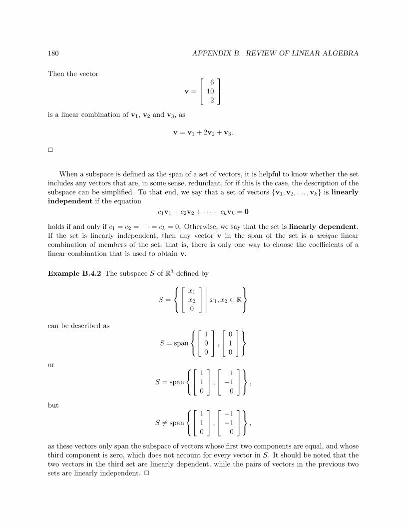
180 APPENDIX B. REVIEW OF LINEAR ALGEBRA
Then the vector
v =
6102
is a linear combination of v1, v2 and v3, as
v = v1 + 2v2 + v3.
2
When a subspace is defined as the span of a set of vectors, it is helpful to know whether the setincludes any vectors that are, in some sense, redundant, for if this is the case, the description of thesubspace can be simplified. To that end, we say that a set of vectors v1,v2, . . . ,vk is linearlyindependent if the equation
c1v1 + c2v2 + · · ·+ ckvk = 0
holds if and only if c1 = c2 = · · · = ck = 0. Otherwise, we say that the set is linearly dependent.If the set is linearly independent, then any vector v in the span of the set is a unique linearcombination of members of the set; that is, there is only one way to choose the coefficients of alinear combination that is used to obtain v.
Example B.4.2 The subspace S of R3 defined by
S =
x1
x2
0
∣∣∣∣∣∣ x1, x2 ∈ R
can be described as
S = span
1
00
, 0
10
or
S = span
1
10
, 1−1
0
,
but
S 6= span
1
10
, −1−1
0
,
as these vectors only span the subspace of vectors whose first two components are equal, and whosethird component is zero, which does not account for every vector in S. It should be noted that thetwo vectors in the third set are linearly dependent, while the pairs of vectors in the previous twosets are linearly independent. 2

B.5. LINEAR TRANSFORMATIONS 181
Example B.4.3 The vectors
v1 =
101
, v2 =
110
are linearly independent. It follows that the only way in which the vector
v =
312
can be expressed as a linear combination of v1 and v2 is
v = 2v1 + v2.
On the other hand, if
v1 =
110
, v2 =
220
, v =
330
,then, because v1 and v2 are linearly dependent, any linear combination of the form c1v1 + c2v2,such that c1 + 2c2 = 3, will equal v. 2
Given a vector space V , if there exists a set of vectors v1,v2, . . . ,vk such that V is the spanof v1,v2, . . . ,vk, and v1,v2, . . . ,vk is linearly independent, then we say that v1,v2, . . . ,vkis a basis of V . Any basis of V must have the same number of elements, k. We call this numberthe dimension of V , which is denoted by dim(V ).
Example B.4.4 The standard basis of R3 is
e1 =
100
, e2 =
010
, e3 =
001
.The set
v1 =
110
, v2 =
1−1
0
, v3 =
001
is also a basis for R3, as it consists of three linearly independent vectors, and the dimension of R3
is three. 2
B.5 Linear Transformations
A function fA : V →W , whose domain V and range W are vector spaces over a field F , is a lineartransformation if it has the properties
fA(x + y) = fA(x) + fA(y), fA(αx) = αfA(x),
where x and y are vectors in V and α is a scalar from F . If V and W are the same vector space,then we say that fA is a linear operator on V .

182 APPENDIX B. REVIEW OF LINEAR ALGEBRA
B.5.1 The Matrix of a Linear Transformation
If V is a vector space of dimension n over a field, such as Rn or Cn, and W is a vector space ofdimension m, then a linear transformation fA with domain V and range W can be represented byan m× n matrix A whose entries belong to the field.
Suppose that the set of vectors v1,v2, . . . ,vn is a basis for V , and the set w1,w2, . . . ,wmis a basis for W . Then, aij is the scalar by which wi is multiplied when applying the function fAto the vector vj . That is,
fA(vj) = a1jw1 + a2jw2 + · · ·+ amjwm =m∑i=1
aijwi.
In other words, the jth column of A describes the image under fA of the vector vj , in terms ofthe coefficients of fA(vj) in the basis w1,w2, . . . ,wm.
If V and W are spaces of real or complex vectors, then, by convention, the bases vjnj=1 andwimi=1 are each chosen to be the standard basis for Rn and Rm, respectively. The jth vector inthe standard basis is a vector whose components are all zero, except for the jth component, whichis equal to one. These vectors are called the standard basis vectors of an n-dimensional space ofreal or complex vectors, and are denoted by ej . From this point on, we will generally assume thatV is Rn, and that the field is R, for simplicity.
Example B.5.1 The standard basis for R3 consists of the vectors
e1 =
100
, e2 =
010
, e3 =
001
.2
B.5.2 Matrix-Vector Multiplication
To describe the action of A on a general vector x from V , we can write
x = x1e1 + x2e2 + · · ·+ xnen =
n∑j=1
xjej .
Then, because A represents a linear function,
fA(x) =
n∑j=1
xjfA(ej) =
n∑j=1
xjaj ,
where aj is the jth column of A.We define the vector y = fA(x) above to be the matrix-vector product of A and x, which
we denote by Ax. Each element of the vector y = Ax is given by
yi = [Ax]i = ai1x1 + ai2x2 + · · ·+ ainxn =n∑j=1
aijxj .
From this definition, we see that the jth column of A is equal to the matrix-vector product Aej .

B.6. MATRIX-MATRIX MULTIPLICATION 183
Example B.5.2 Let
A =
3 0 −11 −4 25 1 −3
, x =
101112
.Then
Ax = 10
315
+ 11
0−41
+ 12
−12−3
=
18−1025
.We see that Ax is a linear combination of the columns of A, with the coefficients of the linearcombination obtained from the components of x. 2
Example B.5.3 Let
A =
3 11 02 4
, x =
[1−1
].
Then the matrix-vector product of A and x is
y = Ax =
3(1) + 1(−1)1(1) + 0(−1)2(1) + 4(−1)
=
21−2
.2
B.5.3 Special Subspaces
Let A be an m × n matrix. Then the range of A, denoted by ran(A), is the set of all vectors ofthe form y = Ax, where x ∈ Rn. It follows that ran(A) is the span of the columns of A, which isalso called the column space of A.
The dimension of ran(A) is called the column rank of A. Similarly, the dimension of the rowspace of A is called the row rank of A. It can be shown that the row rank and column rankare equal; this common value is simply called the rank of A, and is denoted by rank(A). We saythat A is rank-deficient if rank(A) < minm,n; otherwise, we say that A has full rank. It isinteresting to note that any outer product of vectors has rank one.
The null space of A, denoted by null(A), is the set of all vectors x ∈ Rn such that Ax = 0.Its dimension is called the nullity of A. It can be shown that for an m× n matrix A,
dim(null(A)) + rank(A) = n.
B.6 Matrix-Matrix Multiplication
It follows from this definition that a general system of m linear equations in n unknowns can bedescribed in matrix-vector form by the equation
Ax = b,
where Ax is a matrix-vector product of the m×n coefficient matrix A and the vector of unknownsx, and b is the vector of right-hand side values.
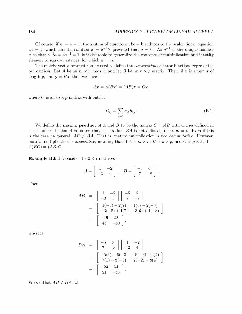
184 APPENDIX B. REVIEW OF LINEAR ALGEBRA
Of course, if m = n = 1, the system of equations Ax = b reduces to the scalar linear equationax = b, which has the solution x = a−1b, provided that a 6= 0. As a−1 is the unique numbersuch that a−1a = aa−1 = 1, it is desirable to generalize the concepts of multiplication and identityelement to square matrices, for which m = n.
The matrix-vector product can be used to define the composition of linear functions representedby matrices. Let A be an m × n matrix, and let B be an n × p matrix. Then, if x is a vector oflength p, and y = Bx, then we have
Ay = A(Bx) = (AB)x = Cx,
where C is an m× p matrix with entries
Cij =
n∑k=1
aikbkj . (B.1)
We define the matrix product of A and B to be the matrix C = AB with entries defined inthis manner. It should be noted that the product BA is not defined, unless m = p. Even if thisis the case, in general, AB 6= BA. That is, matrix multiplication is not commutative. However,matrix multiplication is associative, meaning that if A is m × n, B is n × p, and C is p × k, thenA(BC) = (AB)C.
Example B.6.1 Consider the 2× 2 matrices
A =
[1 −2−3 4
], B =
[−5 67 −8
].
Then
AB =
[1 −2−3 4
] [−5 67 −8
]=
[1(−5)− 2(7) 1(6)− 2(−8)−3(−5) + 4(7) −3(6) + 4(−8)
]=
[−19 2243 −50
],
whereas
BA =
[−5 67 −8
] [1 −2−3 4
]=
[−5(1) + 6(−3) −5(−2) + 6(4)7(1)− 8(−3) 7(−2)− 8(4)
]=
[−23 3431 −46
].
We see that AB 6= BA. 2

B.7. OTHER FUNDAMENTAL MATRIX OPERATIONS 185
Example B.6.2 If
A =
3 11 02 4
, B =
[1 54 −1
],
then the matrix-matrix product of A and B is
C = AB =
3(1) + 1(4) 3(5) + 1(−1)1(1) + 0(4) 1(5) + 0(−1)2(1) + 4(4) 2(5) + 4(−1)
=
7 141 518 6
.It does not make sense to compute BA, because the dimensions are incompatible. 2
B.7 Other Fundamental Matrix Operations
B.7.1 Vector Space Operations
The set of all matrices of size m × n, for fixed m and n, is itself a vector space of dimension mn.The operations of vector addition and scalar multiplication for matrices are defined as follows: IfA and B are m× n matrices, then the sum of A and B, denoted by A+B, is the m× n matrix Cwith entries
cij = aij + bij .
If α is a scalar, then the product of α and an m×n matrix A, denoted by αA, is the m×n matrixB with entries
bij = αaij .
It is natural to identify m×n matrices with vectors of length mn, in the context of these operations.
Matrix addition and scalar multiplication have properties analogous to those of vector additionand scalar multiplication. In addition, matrix multiplication has the following properties relatedto these operations. We assume that A is an m× n matrix, B and D are n× k matrices, and α isa scalar.
• Distributivity: A(B +D) = AB +AD
• Commutativity of scalar multiplication: α(AB) = (αA)B = A(αB)
B.7.2 The Transpose of a Matrix
An n × n matrix A is said to be symmetric if aij = aji for i, j = 1, 2, . . . , n. The n × n matrixB whose entries are defined by bij = aji is called the transpose of A, which we denote by AT .Therefore, A is symmetric if A = AT . More generally, if A is an m×n matrix, then AT is the n×nmatrix B whose entries are defined by bij = aji. The transpose has the following properties:
• (AT )T = A
• (A+B)T = AT +BT
• (AB)T = BTAT
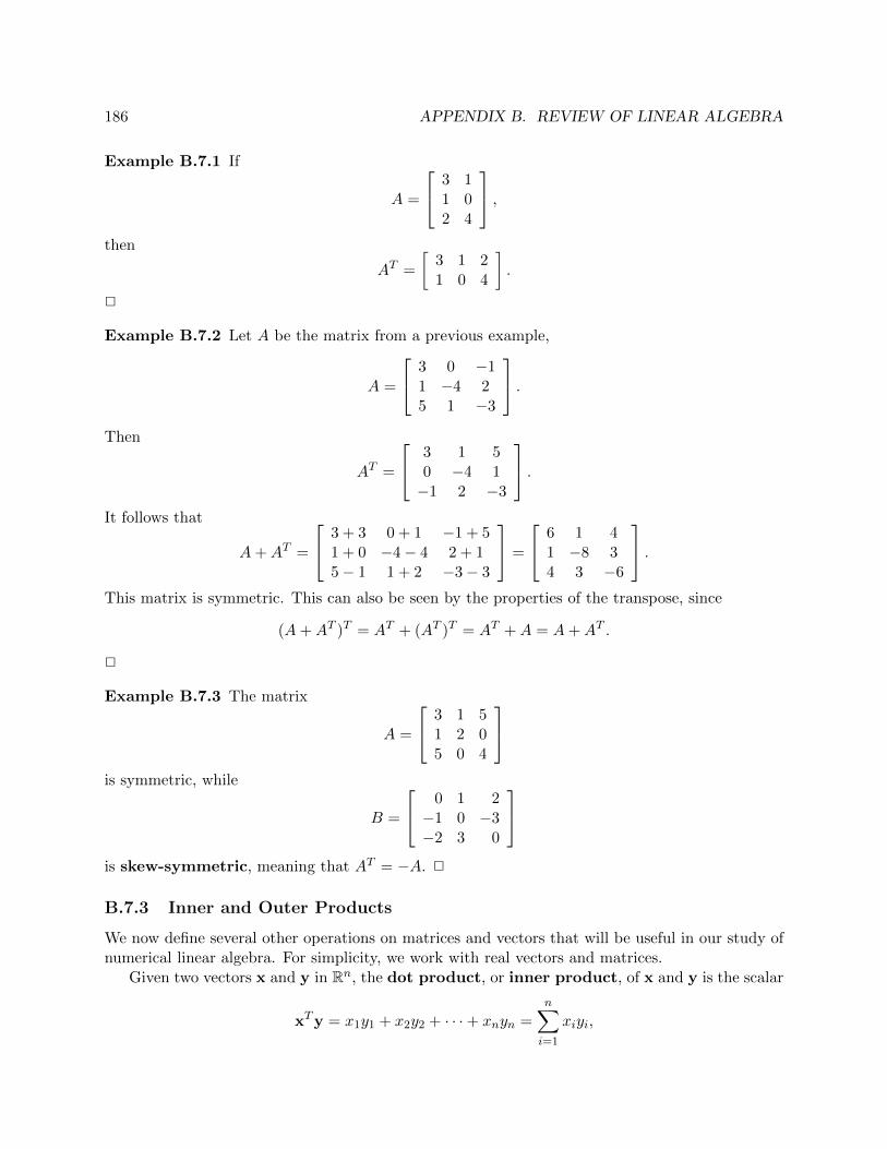
186 APPENDIX B. REVIEW OF LINEAR ALGEBRA
Example B.7.1 If
A =
3 11 02 4
,then
AT =
[3 1 21 0 4
].
2
Example B.7.2 Let A be the matrix from a previous example,
A =
3 0 −11 −4 25 1 −3
.Then
AT =
3 1 50 −4 1−1 2 −3
.It follows that
A+AT =
3 + 3 0 + 1 −1 + 51 + 0 −4− 4 2 + 15− 1 1 + 2 −3− 3
=
6 1 41 −8 34 3 −6
.This matrix is symmetric. This can also be seen by the properties of the transpose, since
(A+AT )T = AT + (AT )T = AT +A = A+AT .
2
Example B.7.3 The matrix
A =
3 1 51 2 05 0 4
is symmetric, while
B =
0 1 2−1 0 −3−2 3 0
is skew-symmetric, meaning that AT = −A. 2
B.7.3 Inner and Outer Products
We now define several other operations on matrices and vectors that will be useful in our study ofnumerical linear algebra. For simplicity, we work with real vectors and matrices.
Given two vectors x and y in Rn, the dot product, or inner product, of x and y is the scalar
xTy = x1y1 + x2y2 + · · ·+ xnyn =n∑i=1
xiyi,

B.7. OTHER FUNDAMENTAL MATRIX OPERATIONS 187
where
x =
x1
x2...xn
, y =
y1
y2...yn
.Note that x and y must both be defined to be column vectors, and they must have the same length.If xTy = 0, then we say that x and y are orthogonal.
Let x ∈ Rm and y ∈ Rn, where m and n are not necessarily equal. The term “inner product”suggests the existence of another operation called the outer product, which is defined by
xyT =
x1y1 x1y2 · · · x1ynx2y1 x2y2 · · · x2yn
......
xmy1 xmy2 · · · xmyn
.Note that whereas the inner product is a scalar, the outer product is an m× n matrix.
Example B.7.4 Let
x =
102
, y =
4−1
3
.Then the inner (dot) product of x and y is
xTy = 1(4) + 0(−1) + 2(3) = 10,
while the outer product of x and y is
xyT =
1(4) 1(−1) 1(3)0(4) 0(−1) 0(3)2(4) 2(−1) 2(3)
=
4 −1 30 0 08 −2 6
.2
Example B.7.5 Let
A =
1 −3 72 5 −84 −6 −9
.To change a11 from 1 to 10, we can perform the outer product update B = A + (10 − 1)e1e
T1 .
Similarly, the outer product update C = B + 5e2eT1 adds 5 to b21, resulting in the matrix
C =
10 −3 77 5 −84 −6 −9
.Note that
e2eT1 =
010
1
010
0
010
0
=
0 0 01 0 00 0 0
.2
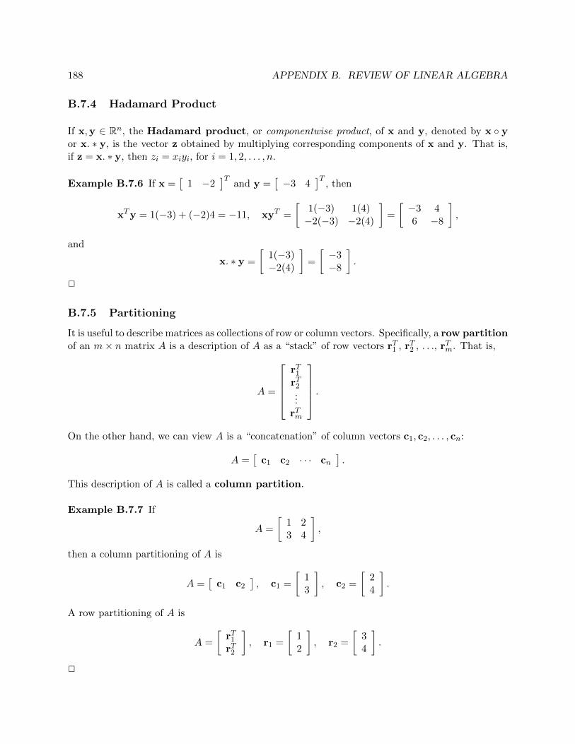
188 APPENDIX B. REVIEW OF LINEAR ALGEBRA
B.7.4 Hadamard Product
If x,y ∈ Rn, the Hadamard product, or componentwise product, of x and y, denoted by x yor x. ∗ y, is the vector z obtained by multiplying corresponding components of x and y. That is,if z = x. ∗ y, then zi = xiyi, for i = 1, 2, . . . , n.
Example B.7.6 If x =[
1 −2]T
and y =[−3 4
]T, then
xTy = 1(−3) + (−2)4 = −11, xyT =
[1(−3) 1(4)−2(−3) −2(4)
]=
[−3 46 −8
],
and
x. ∗ y =
[1(−3)−2(4)
]=
[−3−8
].
2
B.7.5 Partitioning
It is useful to describe matrices as collections of row or column vectors. Specifically, a row partitionof an m× n matrix A is a description of A as a “stack” of row vectors rT1 , rT2 , . . ., rTm. That is,
A =
rT1rT2...
rTm
.On the other hand, we can view A is a “concatenation” of column vectors c1, c2, . . . , cn:
A =[
c1 c2 · · · cn].
This description of A is called a column partition.
Example B.7.7 If
A =
[1 23 4
],
then a column partitioning of A is
A =[
c1 c2
], c1 =
[13
], c2 =
[24
].
A row partitioning of A is
A =
[rT1rT2
], r1 =
[12
], r2 =
[34
].
2
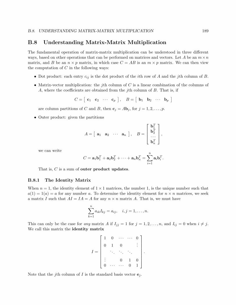
B.8. UNDERSTANDING MATRIX-MATRIX MULTIPLICATION 189
B.8 Understanding Matrix-Matrix Multiplication
The fundamental operation of matrix-matrix multiplication can be understood in three differentways, based on other operations that can be performed on matrices and vectors. Let A be an m×nmatrix, and B be an n× p matrix, in which case C = AB is an m× p matrix. We can then viewthe computation of C in the following ways:
• Dot product: each entry cij is the dot product of the ith row of A and the jth column of B.
• Matrix-vector multiplication: the jth column of C is a linear combination of the columns ofA, where the coefficients are obtained from the jth column of B. That is, if
C =[
c1 c2 · · · cp], B =
[b1 b2 · · · bp
]are column partitions of C and B, then cj = Abj , for j = 1, 2, . . . , p.
• Outer product: given the partitions
A =[
a1 a2 · · · an], B =
bT1bT2· · ·bTn
,we can write
C = a1bT1 + a2b
T2 + · · ·+ anb
Tn =
n∑i=1
aibTi .
That is, C is a sum of outer product updates.
B.8.1 The Identity Matrix
When n = 1, the identity element of 1× 1 matrices, the number 1, is the unique number such thata(1) = 1(a) = a for any number a. To determine the identity element for n× n matrices, we seeka matrix I such that AI = IA = A for any n× n matrix A. That is, we must have
n∑k=1
aikIkj = aij , i, j = 1, . . . , n.
This can only be the case for any matrix A if Ijj = 1 for j = 1, 2, . . . , n, and Iij = 0 when i 6= j.We call this matrix the identity matrix
I =
1 0 · · · · · · 0
0 1 0...
. . .. . .
. . .... 0 1 00 · · · · · · 0 1
.
Note that the jth column of I is the standard basis vector ej .
190 APPENDIX B. REVIEW OF LINEAR ALGEBRA
B.8.2 The Inverse of a Matrix
Given an n× n matrix A, it is now natural to ask whether it is possible to find an n× n matrix Bsuch that AB = BA = I. Such a matrix, if it exists, would then serve as the inverse of A, in thesense of matrix multiplication. We denote this matrix by A−1, just as we denote the multiplicativeinverse of a nonzero number a by a−1. If the inverse of A exists, we say that A is invertible ornonsingular; otherwise, we say that A is singular. If A−1 exists, then we can use it to describethe solution of the system of linear equations Ax = b, for
A−1Ax = (A−1A)x = Ix = x = A−1b,
which generalizes the solution x = a−1b of a single linear equation in one unknown.However, just as we can use the inverse to describe the solution to a system of linear equations,
we can use systems of linear equations to characterize the inverse. Because A−1 satisfies AA−1 = I,it follows from multiplication of both sides of this equation by the jth standard basis vector ej that
Abj = ej , j = 1, 2, . . . , n,
where bj = A−1ej is the jth column of B = A−1. That is, we can compute A−1 by solving nsystems of linear equations of the form Abj = ej , using a method such as Gaussian eliminationand back substitution. If Gaussian elimination fails due to the inability to obtain a nonzero pivotelement for each column, then A−1 does not exist, and we conclude that A is singular.
The inverse of a nonsingular matrix A has the following properties:
• A−1 is unique.
• A−1 is nonsingular, and (A−1)−1 = A.
• If B is also a nonsingular n× n matrix, then (AB)−1 = B−1A−1.
• (A−1)T = (AT )−1. It is common practice to denote the transpose of A−1 by A−T .
Because the set of all n× n matrices has an identity element, matrix multiplication is associative,and each nonsingular n×n matrix has a unique inverse with respect to matrix multiplication that isalso an n×n nonsingular matrix, this set forms a group, which is denoted by GL(n), the generallinear group.
B.9 Triangular and Diagonal Matrices
There are certain types of matrices for which the fundamental problems of numerical linear algebra,solving systems of linear equations or computing eigenvalues and eigenvectors, are relatively easyto solve. We now discuss a few such types.
Let A be an m×n matrix. We define the main diagonal of A to be the entries a11, a22, . . . , app,where p = minm,n. That is, the main diagonal consists of all entries for which the row indexand column index are equal. We then say that A is a diagonal matrix if the only nonzero entriesof A lie on the main diagonal. That is, A is a diagonal matrix if aij = 0 whenever i 6= j.
We say that A is upper triangular if aij = 0 whenever i > j. That is, all nonzero entries ofA are confined to the “upper triangle” of A, which consists of all entries on or “above” the main

B.10. DETERMINANTS 191
diagonal. Similarly, we say that A is lower triangular if aij = 0 whenever i < j. Such a matrixhas all of its nonzero entries on or below the main diagonal.
We will see that a system of linear equations of the form Ax = b is easily solved if A is anupper or lower triangular matrix, and that the eigenvalues of a square matrix A are easy to obtainif A is triangular. As such, certain methods for solving both kinds of problems proceed by reducingA to triangular form.
Example B.9.1 The matrices
U =
1 2 30 4 50 0 6
, L =
1 0 02 3 04 5 6
, D =
1 0 00 2 00 0 3
are upper triangular, lower triangular, and diagonal, respectively. 2
B.10 Determinants
We previously learned that a 2× 2 matrix A is invertible if and only if the quantity a11a22− a12a21
is nonzero. This generalizes the fact that a 1 × 1 matrix a is invertible if and only if its singleentry, a11 = a, is nonzero. We now discuss the generalization of this determination of invertibilityto general square matrices.
The determinant of an n× n matrix A, denoted by det(A) or |A|, is defined as follows:
• If n = 1, then det(A) = a11.
• If n > 1, then det(A) is recursively defined by
det(A) =n∑j=1
aij(−1)i+jMij , 1 ≤ i ≤ n,
where Mij , called a minor of A, is the determinant of the matrix obtained by removing rowi and column j of A.
• Alternatively,
det(A) =
n∑i=1
aij(−1)i+jMij , 1 ≤ j ≤ n.
The expression Aij = (−1)i+jMij is called a cofactor of A.This definition of the determinant, however, does not lead directly to a practical algorithm for
its computation, because it requires O(n!) floating-point operations, whereas typical algorithms formatrix computations run in polynomial time. However, the computational effort can be reduced bychoosing from the multiple formulas for det(A) above. By consistently choosing the row or columnwith the most zeros, the number of operations can be minimized.
However, more practical methods for computing the determinant can be obtained by using itsproperties:
• If any row or column of A has only zero entries, then det(A) = 0.
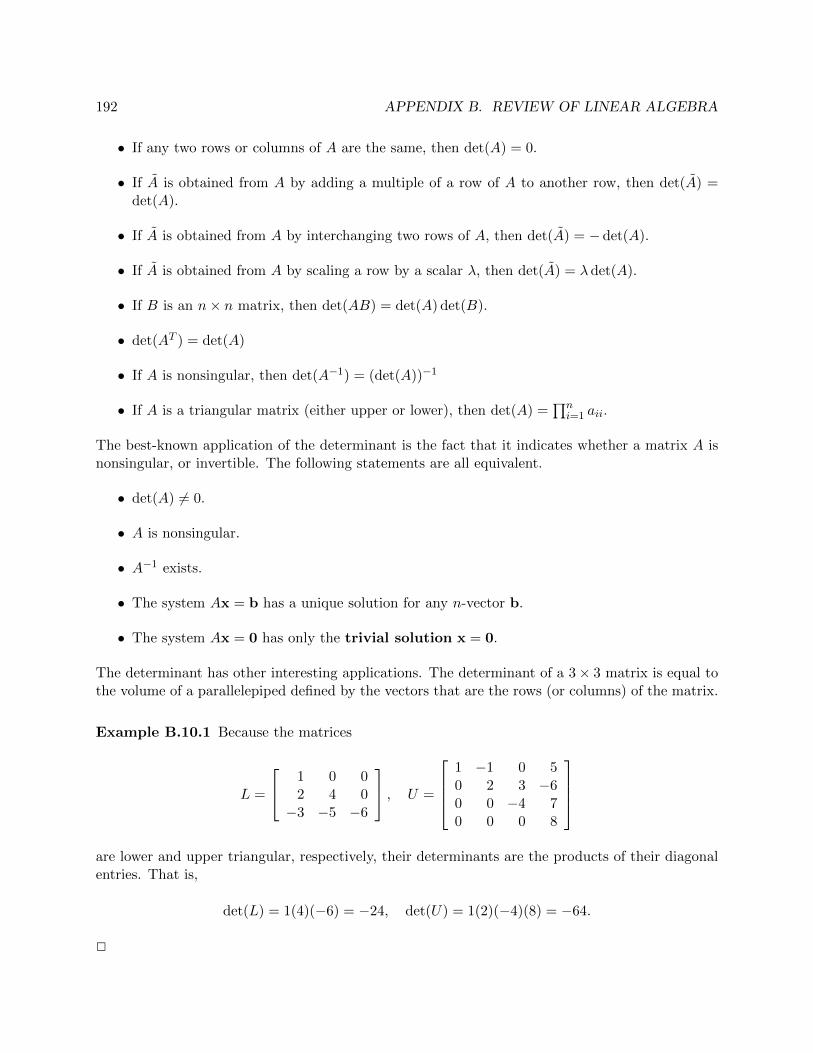
192 APPENDIX B. REVIEW OF LINEAR ALGEBRA
• If any two rows or columns of A are the same, then det(A) = 0.
• If A is obtained from A by adding a multiple of a row of A to another row, then det(A) =det(A).
• If A is obtained from A by interchanging two rows of A, then det(A) = − det(A).
• If A is obtained from A by scaling a row by a scalar λ, then det(A) = λ det(A).
• If B is an n× n matrix, then det(AB) = det(A) det(B).
• det(AT ) = det(A)
• If A is nonsingular, then det(A−1) = (det(A))−1
• If A is a triangular matrix (either upper or lower), then det(A) =∏ni=1 aii.
The best-known application of the determinant is the fact that it indicates whether a matrix A isnonsingular, or invertible. The following statements are all equivalent.
• det(A) 6= 0.
• A is nonsingular.
• A−1 exists.
• The system Ax = b has a unique solution for any n-vector b.
• The system Ax = 0 has only the trivial solution x = 0.
The determinant has other interesting applications. The determinant of a 3× 3 matrix is equal tothe volume of a parallelepiped defined by the vectors that are the rows (or columns) of the matrix.
Example B.10.1 Because the matrices
L =
1 0 02 4 0−3 −5 −6
, U =
1 −1 0 50 2 3 −60 0 −4 70 0 0 8
are lower and upper triangular, respectively, their determinants are the products of their diagonalentries. That is,
det(L) = 1(4)(−6) = −24, det(U) = 1(2)(−4)(8) = −64.
2
B.11. EIGENVALUES 193
B.11 Eigenvalues
Because matrix-vector multiplication is a complicated operation, it is helpful to identify circum-stances under which this operation can be simply described. To that end, we say that a nonzerovector x is an eigenvector of an n× n matrix A if there exists a scalar λ such that
Ax = λx.
The scalar λ is called an eigenvalue of A corresponding to x. Note that although x is required tobe nonzero, it is possible that λ can be zero. It can also be complex, even if A is a real matrix.
If we rearrange the above equation, we have
(A− λI)x = 0.
That is, if λ is an eigenvalue of A, then A−λI is a singular matrix, and therefore det(A−λI) = 0.This equation is actually a polynomial in λ, which is called the characteristic polynomial of A.If A is an n× n matrix, then the characteristic polynomial is of degree n, which means that A hasn eigenvalues, which may repeat.
The following properties of eigenvalues and eigenvectors are helpful to know:
• If λ is an eigenvalue of A, then there is at least one eigenvector of A corresponding to λ
• If there exists an invertible matrix P such that B = PAP−1, then A and B have the sameeigenvalues. We say that A and B are similar, and the transformation PAP−1 is called asimilarity transformation.
• If A is a symmetric matrix, then its eigenvalues are real.
• If A is a skew-symmetric matrix, meaning that AT = −A, then its eigenvalues are eitherequal to zero, or are purely imaginary.
• If A is a real matrix, and λ = u+ iv is a complex eigenvalue of A, then λ = u− iv is also aneigenvalue of A.
• If A is a triangular matrix, then its diagonal entries are the eigenvalues of A.
• det(A) is equal to the product of the eigenvalues of A.
• tr(A), the sum of the diagonal entries of A, is also equal to the sum of the eigenvalues of A.
It follows that any method for computing the roots of a polynomial can be used to obtain theeigenvalues of a matrix A. However, in practice, eigenvalues are normally computed using iterativemethods that employ orthogonal similarity transformations to reduce A to upper triangular form,thus revealing the eigenvalues of A. In practice, such methods for computing eigenvalues are usedto compute roots of polynomials, rather than using polynomial root-finding methods to computeeigenvalues, because they are much more robust with respect to roundoff error.
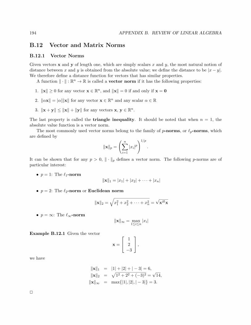
194 APPENDIX B. REVIEW OF LINEAR ALGEBRA
B.12 Vector and Matrix Norms
B.12.1 Vector Norms
Given vectors x and y of length one, which are simply scalars x and y, the most natural notion ofdistance between x and y is obtained from the absolute value; we define the distance to be |x− y|.We therefore define a distance function for vectors that has similar properties.
A function ‖ · ‖ : Rn → R is called a vector norm if it has the following properties:
1. ‖x‖ ≥ 0 for any vector x ∈ Rn, and ‖x‖ = 0 if and only if x = 0
2. ‖αx‖ = |α|‖x‖ for any vector x ∈ Rn and any scalar α ∈ R
3. ‖x + y‖ ≤ ‖x‖+ ‖y‖ for any vectors x, y ∈ Rn.
The last property is called the triangle inequality. It should be noted that when n = 1, theabsolute value function is a vector norm.
The most commonly used vector norms belong to the family of p-norms, or `p-norms, whichare defined by
‖x‖p =
(n∑i=1
|xi|p)1/p
.
It can be shown that for any p > 0, ‖ · ‖p defines a vector norm. The following p-norms are ofparticular interest:
• p = 1: The `1-norm
‖x‖1 = |x1|+ |x2|+ · · ·+ |xn|
• p = 2: The `2-norm or Euclidean norm
‖x‖2 =√x2
1 + x22 + · · ·+ x2
n =√
xHx
• p =∞: The `∞-norm
‖x‖∞ = max1≤i≤n
|xi|
Example B.12.1 Given the vector
x =
12−3
,we have
‖x‖1 = |1|+ |2|+ | − 3| = 6,
‖x‖2 =√
12 + 22 + (−3)2 =√
14,
‖x‖∞ = max|1|, |2|, | − 3| = 3.
2
B.12. VECTOR AND MATRIX NORMS 195
It can be shown that the `2-norm satisfies the Cauchy-Bunyakovsky-Schwarz inequality,also known as simply the Cauchy-Schwarz inequality,
|xTy| ≤ ‖x‖2‖y‖2
for any vectors x, y ∈ Rn. This inequality is useful for showing that the `2-norm satisfies thetriangle inequality. It is a special case of the Holder inequality
|xTy| ≤ ‖x‖p‖y‖q,1
p+
1
q= 1.
We will prove the Cauchy-Schwarz inequality for vectors in Rn; the proof can be generalized toa complex vector space. For x,y ∈ Rn and c ∈ R, with y 6= 0, we have
(x− cy)T (x− cy) = ‖x− cy‖22 ≥ 0.
It follows from the properties of the inner product that
0 ≤ (x− cy)T (x− cy)
≤ xTx− xT (cy)− (cy)Tx + (cy)T (cy)
≤ ‖x‖22 − 2cxTy + c2‖y‖22.
We now try to find the value of c that minimizes this expression. Differentiating with respect to cand equating to zero yields the equation
−2xTy + 2c‖y‖22 = 0,
and therefore the minimum occurs when c = xTy/‖y‖22. It follows that
0 ≤ ‖x‖22 − 2cxTy + c2‖y‖2
≤ ‖x‖22 − 2xTy
‖y‖22xTy +
(xTy)2
‖y‖42‖y‖22
≤ ‖x‖22 − 2(xTy)2
‖y‖22+
(xTy)2
‖g‖2
≤ ‖x‖22 −(xTy)2
‖y‖22.
It follows that
(xTy)2 ≤ ‖x‖22‖y‖22.
Taking the square root of both sides yields the Cauchy-Schwarz inequality.Now that we have defined various notions of the size, or magnitude, of a vector, we can discuss
distance and convergence. Given a vector norm ‖ ·‖, and vectors x,y ∈ Rn, we define the distancebetween x and y, with respect to this norm, by ‖x−y‖. Then, we say that a sequence of n-vectorsx(k)∞k=0 converges to a vector x if
limk→∞
‖x(k) − x‖ = 0.
196 APPENDIX B. REVIEW OF LINEAR ALGEBRA
That is, the distance between x(k) and x must approach zero. It can be shown that regardless ofthe choice of norm, x(k) → x if and only if
x(k)i → xi, i = 1, 2, . . . , n.
That is, each component of x(k) must converge to the corresponding component of x. This is dueto the fact that for any vector norm ‖ · ‖, ‖x‖ = 0 if and only if x is the zero vector.
Because we have defined convergence with respect to an arbitrary norm, it is important to knowwhether a sequence can converge to a limit with respect to one norm, while converging to a differentlimit in another norm, or perhaps not converging at all. Fortunately, for p-norms, this is never thecase. We say that two vector norms ‖ · ‖α and ‖ · ‖β are equivalent if there exists constants C1
and C2, that are independent of x, such that for any vector x ∈ Rn,
C1‖x‖α ≤ ‖x‖β ≤ C2‖x‖α.
It follows that if two norms are equivalent, then a sequence of vectors that converges to a limitwith respect to one norm will converge to the same limit in the other. It can be shown that all`p-norms are equivalent. In particular, if x ∈ Rn, then
‖x‖2 ≤ ‖x‖1 ≤√n‖x‖2,
‖x‖∞ ≤ ‖x‖2 ≤√n‖x‖∞,
‖x‖∞ ≤ ‖x‖1 ≤ n‖x‖∞.
We will now prove the equivalence of ‖ · ‖1 and ‖ · ‖2. Let x ∈ Rn. First, we have
‖x‖22 =n∑i=1
|xi|2 ≤n∑
i,j=1
|xi||xj | ≤ ‖x‖21,
and therefore ‖x‖2 ≤ ‖x1‖1. Then, we define the vector y by
yi =
1 xi ≥ 0−1 xi < 0
.
It follows that ‖x1‖ = yTx. By the Cauchy-Schwarz inequality,
‖x‖1 = yTx ≤ ‖y‖2‖x‖2 ≤√n‖x‖2
and the equivalence of the norms has been established.
B.12.2 Matrix Norms
It is also very useful to be able to measure the magnitude of a matrix, or the distance betweenmatrices. However, it is not sufficient to simply define the norm of an m×n matrix A as the normof an mn-vector x whose components are the entries of A. We instead define a matrix norm tobe a function ‖ · ‖ : Rm×n → R that has the following properties:
• ‖A‖ ≥ 0 for any A ∈ Rm×n, and ‖A‖ = 0 if and only if A = 0

B.12. VECTOR AND MATRIX NORMS 197
• ‖αA‖ = |α|‖A‖ for any m× n matrix A and scalar α
• ‖A+B‖ ≤ ‖A‖+ ‖B‖ for any m× n matrices A and B
Another property that is often, but not always, included in the definition of a matrix norm is thesubmultiplicative property: if A is m× n and B is n× p, we require that
‖AB‖ ≤ ‖A‖‖B‖.
This is particularly useful when A and B are square matrices.Any vector norm induces a matrix norm. It can be shown that given a vector norm, defined
appropriately for m-vectors and n-vectors, the function ‖ · ‖ : Rm×n → R defined by
‖A‖ = supx 6=0
‖Ax‖‖x‖
= max‖x‖=1
‖Ax‖
is a matrix norm. It is called the natural, or induced, matrix norm. Furthermore, if the vectornorm is a `p-norm, then the induced matrix norm satisfies the submultiplicative property.
The following matrix norms are of particular interest:
• The `1-norm:
‖A‖1 = max‖x‖1=1
‖Ax‖1 = max1≤j≤n
m∑i=1
|aij |.
That is, the `1-norm of a matrix is its maximum column sum of |A|. To see this, let x ∈ Rnsatisfy ‖x‖1 = 1. Then
‖Ax‖1 =
m∑i=1
|(Ax)i|
=
m∑i=1
∣∣∣∣∣∣n∑j=1
aijxj
∣∣∣∣∣∣≤
n∑j=1
|xj |
(m∑i=1
|aij |
)
≤n∑j=1
|xj | max1≤j≤n
(m∑i=1
|aij |
)
≤ max1≤j≤n
(m∑i=1
|aij |
).
Equality is achieved if x = eJ , where the index J satisfies
max1≤j≤n
(m∑i=1
|aij |
)=
m∑i=1
|aiJ |.
It follows that the maximum column sum of |A| is equal to the maximum of ‖Ax‖1 takenover all the set of all unit 1-norm vectors.

198 APPENDIX B. REVIEW OF LINEAR ALGEBRA
• The `∞-norm:
‖A‖∞ = max‖x‖∞=1
‖Ax‖∞ = max1≤i≤m
n∑j=1
|aij |.
That is, the `∞-norm of a matrix is its maximum row sum. This formula can be obtained ina similar manner as the one for the matrix 1-norm.
• The `2-norm:
‖A‖2 = max‖x‖2=1
‖Ax‖2.
To obtain a formula for this norm, we note that the function
g(x) =‖Ax‖22‖x‖22
has a local maximum or minimum whenever x is a unit `2-norm vector (that is, ‖x‖2 = 1)that satisfies
ATAx = ‖Ax‖22x,
as can be shown by differentiation of g(x). That is, x is an eigenvector of ATA, with corre-sponding eigenvalue ‖Ax‖22 = g(x). We conclude that
‖A‖2 = max1≤i≤n
√λi(ATA). (B.2)
That is, the `2-norm of a matrix is the square root of the largest eigenvalue of ATA, which isguaranteed to be nonnegative, as can be shown using the vector 2-norm. We see that unlikethe vector `2-norm, the matrix `2-norm is much more difficult to compute than the matrix`1-norm or `∞-norm.
• The Frobenius norm:
‖A‖F =
m∑i=1
n∑j=1
a2ij
1/2
. (B.3)
It should be noted that the Frobenius norm is not induced by any vector `p-norm, but itis equivalent to the vector `2-norm in the sense that ‖A‖F = ‖x‖2 where x is obtained byreshaping A into a vector.
Like vector norms, matrix norms are equivalent. For example, if A is an m× n matrix, we have
‖A‖2 ≤ ‖A‖F ≤√n‖A‖2,
1√n‖A‖∞ ≤ ‖A‖2 ≤
√m‖A‖∞,
1√m‖A‖1 ≤ ‖A‖2 ≤
√n‖A‖1.
B.12. VECTOR AND MATRIX NORMS 199
Example B.12.2 Let
A =
1 2 30 1 0−1 0 4
.Then
‖A‖1 = max|1|+ |0|+ | − 1|, |2|+ |1|+ |0|, |3|+ |0|+ |4| = 7,
and‖A‖∞ = max|1|+ |2|+ |3|, |0|+ |1|+ |0|, | − 1|+ |0|+ |4| = 6.
2
B.12.3 Function Spaces and Norms
We now define norms on more general vector spaces. Let V be a vector space over the field of realnumbers R. A norm on V is a function ‖ · ‖ : V → R that has the following properties:
1. ‖f‖ ≥ 0 for all f ∈ V, and ‖f‖ = 0 if and only if f is the zero vector of V.
2. ‖cf‖ = |c|‖f‖ for any vector f ∈ V and any scalar c ∈ R.
3. ‖f + g‖ ≤ ‖f‖+ ‖g‖ for all f, g ∈ V.
The last property is known as the triangle inequality. A vector space V, together with a norm‖ · ‖, is called a normed vector space or normed linear space. In particular, we are interestedin working with function spaces, which are vector spaces in which the vectors are functions.
Example B.12.3 The space C[a, b] of functions that are continuous on the interval [a, b] is anormed vector space with the norm
‖f‖∞ = maxa≤x≤b
|f(x)|,
known as the ∞-norm or maximum norm. 2
Example B.12.4 The space C[a, b] can be equipped with a different norm, such as
‖f‖2 =
(∫ b
a|f(x)|2w(x) dx
)1/2
,
where the weight function w(x) is positive and integrable on (a, b). It is allowed to be singular atthe endpoints, as will be seen in certain examples. This norm is called the L2-norm or weightedL2-norm. 2
The L2-norm and L∞-norm are related as follows:
‖f‖2 ≤W‖f‖∞, W = ‖1‖2.
However, unlike the L∞-norm and L2-norm defined for the vector space Rn, these norms are notequivalent in the sense that a function that has a small L2-norm necessarily has a small L∞-norm.
200 APPENDIX B. REVIEW OF LINEAR ALGEBRA
In fact, given any ε > 0, no matter how small, and any M > 0, no matter how large, there exists afunction f ∈ C[a, b] such that
‖f‖2 < ε, ‖f‖∞ > M.
We say that a function f is absolutely continuous on [a, b] if its derivative is finite almosteverywhere in [a, b] (meaning that it is not finite on at most a subset of [a, b] that has measurezero), is integrable on [a, b], and satisfies∫ x
af ′(s) dx = f(x)− f(a), a ≤ x ≤ b.
Any continuously differentiable function is absolutely continuous, but the converse is not necessarilytrue.
Example B.12.5 For example, f(x) = |x| is absolutely continuous on any interval of the form[−a, a], but it is not continuously differentiable on such an interval. 2
Next, we define the Sobolev spaces Hk(a, b) as follows. The space H1(a, b) is the set ofall absolutely continuous functions on [a, b] whose derivatives belong to L2(a, b). Then, for k > 1,Hk(a, b) is the subset of Hk−1(a, b) consisting of functions whose (k−1)st derivatives are absolutelycontinuous, and whose kth derivatives belong to L2(a, b). If we denote by Ck[a, b] the set of allfunctions defined on [a, b] that are k times continuously differentiable, then Ck[a, b] is a propersubset of Hk(a, b). For example, any piecewise linear belongs to H1(a, b), but does not generallybelong to C1[a, b].
Example B.12.6 The function f(x) = x3/4 belongs to H1(0, 1) because f ′(x) = 34x−1/4 is inte-
grable on [0, 1], and also square-integrable on [0, 1], since∫ 1
0|f ′(x)|2 dx =
∫ 1
0
9
16x−1/2 =
9
8x1/2
∣∣∣∣10
=9
8.
However, f /∈ C1[a, b], because f ′(x) is singular at x = 0. 2
B.13 Inner Product Spaces
Recall that two m-vectors u = 〈u1, u2, . . . , um〉 and v = 〈v1, v2, . . . , vm〉 are orthogonal if
u · v =
m∑i=1
uivi = 0,
where u · v is the dot product, or inner product, of u and v.By viewing functions defined on an interval [a, b] as infinitely long vectors, we can generalize
the inner product, and the concept of orthogonality, to functions. To that end, we define the innerproduct of two real-valued functions f(x) and g(x) defined on the interval [a, b] by
〈f, g〉 =
∫ b
af(x)g(x) dx.
B.14. CONVERGENCE 201
Then, we say f and g are orthogonal with respect to this inner product if 〈f, g〉 = 0.
In general, an inner product on a vector space V over R, be it continuous or discrete, has thefollowing properties:
1. 〈f + g, h〉 = 〈f, h〉+ 〈g, h〉 for all f, g, h ∈ V
2. 〈cf, g〉 = c〈f, g〉 for all c ∈ R and all f ∈ V
3. 〈f, g〉 = 〈g, f〉 for all f, g ∈ V
4. 〈f, f〉 ≥ 0 for all f ∈ V, and 〈f, f〉 = 0 if and only if f = 0.
This inner product can be used to define the norm of a function, which generalizes the conceptof the magnitude of a vector to functions, and therefore provides a measure of the “magnitude” ofa function. Recall that the magnitude of a vector v, denoted by ‖v‖, can be defined by
‖v‖ = (v · v)1/2.
Along similar lines, we define the L2-norm of a function f(x) defined on [a, b] by
‖f‖2 = (〈f, f〉)1/2 =
(∫ b
a[f(x)]2 dx
)1/2
.
It can be verified that this function does in fact satisfy the properties required of a norm.
One very important property that ‖·‖2 has is that it satisfies the Cauchy-Schwarz inequality
|〈f, g〉| ≤ ‖f‖2‖g‖2, f, g ∈ V.
This can be proven by noting that for any scalar c ∈ R,
c2‖f‖22 + 2c〈f, g〉+ ‖g‖22 = ‖cf + g‖22 ≥ 0.
The left side is a quadratic polynomial in c. In order for this polynomial to not have any negativevalues, it must either have complex roots or a double real root. This is the case if the discriminantsatisfies
4〈f, g〉2 − 4‖f‖22‖g‖22 ≤ 0,
from which the Cauchy-Schwarz inequality immediately follows. By setting c = 1 and applying thisinequality, we immediately obtain the triangle-inequality property of norms.
B.14 Convergence
We have learned in Section B.12 what it means for a sequence of vectors to converge to a limit.However, using the definition alone, it may still be difficult to determine, conclusively, whethera given sequence of vectors converges. For example, suppose a sequence of vectors is defined asfollows: we choose the initial vector x(0) arbitrarily, and then define the rest of the sequence by
x(k+1) = Ax(k), k = 0, 1, 2, . . .

202 APPENDIX B. REVIEW OF LINEAR ALGEBRA
for some matrix A. Such a sequence actually arises in the study of the convergence of variousiterative methods for solving systems of linear equations.
An important question is whether a sequence of this form converges to the zero vector. Thiswill be the case if
limk→∞
‖x(k)‖ = 0
in some vector norm. From the definition of x(k), we must have
limk→∞
‖Akx(0)‖ = 0.
From the submultiplicative property of matrix norms,
‖Akx(0)‖ ≤ ‖A‖k‖x(0)‖,
from which it follows that the sequence will converge to the zero vector if ‖A‖ < 1. However, thisis only a sufficient condition; it is not necessary.
A sufficient and necessary condition can be described in terms of the eigenvalues of A, asdescribed in Section B.11. It can be shown that if each eigenvalue λ of a matrix A satisfies |λ| < 1,then, for any vector x,
limk→∞
Akx = 0.
Furthermore, the converse of this statement is also true: if there exists a vector x such that Akxdoes not approach 0 as k →∞, then at least one eigenvalue λ of A must satisfy |λ| ≥ 1.
Therefore, it is through the eigenvalues of A that we can describe a necessary and sufficientcondition for a sequence of vectors of the form x(k) = Akx(0) to converge to the zero vector.Specifically, we need only check if the magnitude of the largest eigenvalue is less than 1. Forconvenience, we define the spectral radius of A, denoted by ρ(A), to be max |λ|, where λ is aneigenvalue of A. We can then conclude that the sequence x(k) = Akx(0) converges to the zero vectorif and only if ρ(A) < 1.
Example B.14.1 Let
A =
2 3 10 4 50 0 1
.Then
A− 2I =
2− 2 3 10 4− 2 50 0 1− 2
=
0 3 10 2 50 0 −1
.Because A− 2I has a column of all zeros, it is singular. Therefore, 2 is an eigenvalue of A. In fact,
Ae1 = 2e1, so e1 =[
1 0 0]T
is an eigenvector.Because A is upper triangular, its eigenvalues are the diagonal elements, 2, 4 and 1. Because
the largest eigenvalue in magnitude is 4, the spectral radius of A is ρ(A) = 4. 2
The spectral radius is closely related to natural (induced) matrix norms. Let λ be the largesteigenvalue of A, with x being a corresponding eigenvector. Then, for any natural matrix norm ‖ ·‖,we have
ρ(A)‖x‖ = |λ|‖x‖ = ‖λx‖ = ‖Ax‖ ≤ ‖A‖‖x‖.
B.15. DIFFERENTIATION OF MATRICES 203
Therefore, we have ρ(A) ≤ ‖A‖. When A is symmetric, we also have
‖A‖2 = ρ(A).
For a general matrix A, we have
‖A‖2 = [ρ(ATA)]1/2,
which can be seen to reduce to ρ(A) when AT = A, since, in general, ρ(Ak) = ρ(A)k.
Because the condition ρ(A) < 1 is necessary and sufficient to ensure that limk→∞Akx = 0, it
is possible that such convergence may occur even if ‖A‖ ≥ 1 for some natural norm ‖ · ‖. However,if ρ(A) < 1, we can conclude that
limk→∞
‖Ak‖ = 0,
even though limk→∞ ‖A‖k may not even exist.
In view of the definition of a matrix norm, that ‖A‖ = 0 if and only if A = 0, we can concludethat if ρ(A) < 1, then Ak converges to the zero matrix as k → ∞. In summary, the followingstatements are all equivalent:
1. ρ(A) < 1
2. limk→∞ ‖Ak‖ = 0, for any natural norm ‖ · ‖
3. limk→∞(Ak)ij = 0, i, j = 1, 2, . . . , n
4. limk→∞Akx = 0
These results are very useful for analyzing the convergence behavior of various iterative methodsfor solving systems of linear equations.
B.15 Differentiation of Matrices
Suppose that A(t) is an m×n matrix in which each entry is a function of a parameter t. Then thematrix A′(t), or dA/dt, is the m× n matrix obtained by differentiating each entry with respect tot. That is, [
dA(t)
dt
]ij
=d
dt[aij(t)].
Matrices obey differentiation rules that are analogous to differentiation rules for functions, but therules of matrix-matrix multiplication must be taken into account. For example, if A(t) is an m×nmatrix and B is an n× p matrix, then
d
dt[A(t)B(t)] =
d
dt[A(t)]B(t) +A(t)
d
dt[B(t)],
and if A(t) is a nonsingular n× n matrix, then
d
dt[A(t)−1] = −A(t)−1 d
dt[A(t)]A(t)−1.
204 APPENDIX B. REVIEW OF LINEAR ALGEBRA
It is also useful to know how to differentiate functions of vectors with respect to their compo-nents. Let A be an n× n matrix and x ∈ Rn. Then, we have
∇(xTAx
)= (A+AT )x, ∇(xTb) = b.
These formulas are useful in problems involving minimization of functions of x, such as the least-squares problem, which entails approximately solving a system of m equations in n unknowns,where typically m > n.

Bibliography
[1] Abramowitz, M. and Stegun, I. A., Eds.: Handbook of Mathematical Functions with Formulas,Graphs, and Mathematical Tables, 9th printing. New York: Dover (1972).
[2] Ahlberg, J. H., Nilson, E. N. and Walsh, J. L.: The Theory of Splines and Their Applications,Academic Press, New York (1967).
[3] Aitken, A. C.: “On interpolation by iteration of proportional parts, without the use of differ-ences”. Proc. Edinburgh Math. Soc. 3(2) (1932), p. 56-76.
[4] Alefeld, G. and Herzberger, J.: Introduction to Interval Computations, Academic Press, NewYork (1983).
[5] Anderson, E., Bai, Z., Bischof, C., Blackford, S., Demmel, J., Dongarra, J., DuCroz, J.,Greenbaum, A., Hammarling, S., McKenney, A. and Sorenson, D.: LAPACK Users’ Guide, 3rded., SIAM, Philadelphia (1999).
[6] Arfken, G. B., Weber, H. J. and Harris, F. E.: Mathematical Methods for Physicists: AComprehensive Guide, 7th ed., Academic Press, New York (2012).
[7] Ascher, U. M.: Numerical Methods for Evolutionary Differential Equations, SIAM, Philadel-phia (2008).
[8] Ascher, U. M. and Greif, C.: A First Course in Numerical Methods, SIAM, Philadelphia(2011).
[9] Ascher, U. M., Mattheij, R. M. and Russell, R. D.: Numerical Solution of Boundary ValueProblems for Ordinary Differential Equations, SIAM, Philadelphia (1995).
[10] Ascher, U. M. and Petzold, L. R.: Computer Methods for Ordinary Differential Equations andDifferential-Algebraic Equations, SIAM, Philadelphia (1998).
[11] Atkinson, K..: Introduction to Numerical Analysis, 2nd ed., John Wiley & Sons, New York(1989).
[12] Bailey, P. B., Shampine, L. F. and Waltman, P. E.: Nonlinear Two Point Boundary ValueProblems, Academic Press, New York (1968).
[13] Banach, S.: “Sur les operations dans les ensembles abstraits et leur application aux equationsintegrales.” Fund. Math. 3 (1922), p. 133-181.
205

206 BIBLIOGRAPHY
[14] Bartels, R., Beatty, J. and Barksy, B.: An Introduction to Splines for Use in Computer Graph-ics and Geometric Modeling, Morgan Kaufmann, Los Altos, CA (1987).
[15] Bashforth, F. and Adams, J. C.: An Attempt to test the Theories of Capillary Action bycomparing the theoretical and measured forms of drops of fluid. With an explanation of themethod of integration employed in constructing the tables which give the theoretical forms ofsuch drops, Cambridge University Press (1883).
[16] Baveley, C. and Stewart, G. W.: “An Algorithm for Computing Reducing Subspaces by BlockDiagonalization“, SIAM J. Num. Anal. 16 (1979), p. 359-367.
[17] Berrut, J.-P. and Trefethen, L. N.: “Barycentric Lagrange Interpolation”. SIAM Review 46(3)(2004), p. 501-517.
[18] Berry, M. W. and Browne, M.: Understanding Search Engines: Mathematical Modeling andText Retrieval, 2nd ed., SIAM, Philadelphia (2005).
[19] Betounes, D.: Differential Equations: Theory and Applications, 2nd ed., Springer-Verlag, NewYork (2010).
[20] Birkhoff, G. and De Boor, C.: “Error bounds for spline interpolation”, Journal of Mathematicsand Mechanics 13 (1964), p. 827-836.
[21] Birkhoff, G. and Rota, G.: Ordinary differential equations, 4th ed., John Wiley & Sons, NewYork, (1989)
[22] Bjorck, A: Numerical Methods for Least Squares Problems, SIAM, Philadelphia (1996).
[23] Blum, L., Cucker, F., Shub, M., and Smale, S.: Complexity and Real Computation, Springer-Verlag, Berlin (2001).
[24] Bogacki, P. and Shampine, L. F.: “A 3(2) pair of Runge-Kutta formulas”, Applied MathematicsLetters 2(4) (1989), p. 321-325.
[25] Boyce, W. E. and DiPrima, R. C.: Elementary Differential Equations and Boundary ValueProblems, 10th ed., John Wiley & Sons, New York (2013).
[26] Boyd, J. P.: Chebyshev and Fourier Spectral Methods, 2nd ed., Dover, New York (2001).
[27] Braun, M.: Differential Equations and Their Applications, 4th ed., Springer-Verlag, New York(1993).
[28] Brezinski, C. and Redivo Zaglia, M.: Extrapolation Methods: Theory and Practice, Elsevier,New York (1991).
[29] Briggs, W. L., Henson, V. E. and McCormick, S. F.: A Multigrid Tutorial, 2nd ed., SIAM,Philadelphia (2000).
[30] Brouwer, L. E. J.: “Uber Abbildungen von Mannigfaltigkeiten”, Mathematische Annalen 71(1911), p. 97-115.

BIBLIOGRAPHY 207
[31] Burden, R. L. and Faires, J. D.: Numerical Analysis, 9th ed., Brooks/Cole, Pacific Grove, CA(2004).
[32] Canuto, C., Hussaini, M. Y., Quarteroni, A. and Zang, Th. A.: Spectral Methods: Fundamen-tals in Single Domains, Springer-Verlag, New York (2006).
[33] Cheney, W. and Kincaid, D.: Numerical Mathematics and Computing, 6th ed., Brooks/Cole,Pacific Grove, CA (2008).
[34] Cipra, B. A.: “The Best of the 20th Century: Editors Name Top 10 Algorithms”, SIAM News33(4) (2000).
[35] Conte, S. D. and de Boor, C.: Elementary Numerical Analysis: An Algorithmic Approach, 3rded., McGraw-Hill, New York (1981).
[36] Cools, R.: “Constructing cubature formulae: the science behind the art”, Acta Numerica 6(1997), p. 1-54.
[37] Cormen, T. H., Leiserson, C. E. and Rivest, R. L.: Introduction to Algorithms, 3rd ed., MITPress, Cambridge, MA (2009).
[38] Dahlquist, G.: “A special stability problem for linear multistep methods”, BIT 3 (1963), p.27-43.
[39] Dahlquist, G. and Bjorck, A.: Numerical Methods, Prentice-Hall, Englewood Cliffs, NJ (1974).
[40] Daubechies, I: Ten Lectures on Wavelets, SIAM, Philadelphia (1992).
[41] Davis, P. J.: Interpolation and Approximation, Dover, New York (1975).
[42] Davis, P. J. and Rabinowitz, P.: Methods of Numerical Integration, 2nd ed., Academic Press,New York (1985).
[43] Davis, T. A.: Direct Methods for Sparse Linear Systems, SIAM, Philadelphia (2006).
[44] de Boor, C.: A Practical Guide to Splines, 2nd ed., Springer-Verlag, New York (1984).
[45] Demmel, J. W.: Applied Numerical Linear Algebra, SIAM (1997).
[46] Demmel, J. W., Heath, M. T. and van der Vorst, H. H.: “Parallel numerical linear algebra”,Acta Numerica 2 (1993), p. 111-197.
[47] Dierckx, P.: Curve and Surface Fitting with Splines, Oxford University Press, New York (1993).
[48] Dongarra, J. J., Bunch, J. R., Moler, C. B. and Stewart, G. W.: LINPACK User’s Guide, 2nded., SIAM, Philadelphia (1979).
[49] Dongarra, J. J., DuCroz, J., Duff, I. S. and Hammarling, S.: “A set of level-3 basic linearalgebra subprograms”, ACM Trans. Math. Software 16 (1990), p. 1-28.
[50] Dongarra, J. J., DuCroz, J., Hammarling, S. and Hanson, R. J.: “An extended set of Fortranbasic linear algebra subprograms”, ACM Trans. Math. Software 14 (1988), p. 1-32.

208 BIBLIOGRAPHY
[51] Dongarra, J. J., Duff, I. S., Sorenson, D. C. and van der Vorst, H. H. Numerical Linear Algebrafor High-Performance Computers, SIAM, Philadelphia (1998).
[52] Dongarra, J. J., Gustavson, F. G. and Karp, A.: “Implementing linear algebra algorithms fordense matrices on a vector pipeline machine”, SIAM Review 26 (1984), p. 91-112.
[53] Dongarra, J. J. and Sorensen, D. C.: “A Fully Parallel Algorithm for the Symmetric EigenvalueProblem”, SIAM J. Sci. and Stat. Comp. 8 (1987), p. s139-s154.
[54] Dormand, J. R. and Prince, P. J.: “A family of embedded Runge-Kutta formulae”, Journal ofComputational and Applied Mathematics 6 (1) (1980), p. 19-26.
[55] Driscoll, T. A., Hale, N. and Trefethen, L. N., editors: Chebfun Guide, Pafnuty Publications,Oxford (2014).
[56] Edelman, A. and Murakami, H.: “Polynomial roots from companion matrix eigenvalues”,Mathematics of Computation 64(210) (1995), p. 763-776.
[57] Elman, H. C., Silvester, D. J. and Wathen, A. J.: Finite Elements and Fast Iterative Solvers:With Applications in Incompressible Fluid Dynamics, Oxford University Press, New York(2005).
[58] Engels, H.: Numerical Quadrature and Cubature, Academic Press, New York (1980).
[59] Eriksson, K., Estep, D., Hansbo, P. and Johnson, C.: Computational Differential Equations,Cambridge University Press, New York (1996).
[60] Evans, G.: Practical Numerical Integration, John Wiley & Sons, New York (1993).
[61] Farebrother, R. W.: Linear Least Squares Computations, Marcel Dekker, New York (1988).
[62] Farin, G. Curves and Surfaces for Computer Aided Geometric Design, 2nd ed., AcademicPress, New York (1990).
[63] Fehlberg, E.: “Klassische Runge-Kutta Formeln vierter und niedrigerer Ordnung mitSchrittweiten-Kontrolle und ihre Anwendung auf Wrmeleitungsprobleme”, Computing 6(1970), p. 61-71.
[64] Fletcher, R.: Practical methods of optimization (2nd ed.), New York: John Wiley & Sons(1987).
[65] Foster, L. V.: “Gaussian elimination with partial pivoting can fail in practice”, SIAM J. MatrixAnal. Appl. 15 (1994), p. 1354-1362.
[66] Fox, L.: The Numerical Solution of Two-Point Boundary Problems, Dover, New York (1990).
[67] Fox, L. and Parker, I. B.: Chebyshev Polynomials in Numerical Analysis, Oxford UniversityPress, New York (1968).
[68] Francis, J. G. F.: “The QR Transformation: A Unitary Analogue to the LR Transformation,Parts I and II”. Comp. J. 4 (1961), p. 265-272, 332-345.
BIBLIOGRAPHY 209
[69] Frigo, M. and Johnson, S. G.: “The Design and Implementation of FFTW3”, Proceedings ofthe IEEE 93(2) (2005), p. 216?231.
[70] Fritsch, F. N., Kahaner, D. K. and Lyness, J. N.: “Double integration using one-dimensionaladaptive quadrature routines: A software interface problem”, ACM Trans. Math. Software 7(1981), p. 46-75.
[71] Gander, W. and Gautschi, W.: “Adaptive quadrature–revisited”, BIT 40 (2000), p. 84-101.
[72] Garbow, B. S., Boyle, J. M., Dongarra, J. J. and Moler, C. B.: Matrix Eigensystem Routines:EISPACK Guide Extension, Springer-Verlag, New York (1972).
[73] Garon, E. M. and Lambers, J. V.: “Modeling the Diffusion of Heat Energy within Compos-ites of Homogeneous Materials using the Uncertainty Principle”, Computational and AppliedMathematics (2018), in press.
[74] Gautschi, W. Numerical Analysis: an Introduction, Birkhauser, Boston, MA, 1997.
[75] Gear, C. W.: Numerical Initial Value Problems in Ordinary Differential Equations, Prentice-Hall, Englewood Cliffs, NJ (1971)
[76] Ghizzetti, A. and Ossicini, A.: Quadrature Formulae, Academic Press, New York (1970).
[77] Gill, P. E., Murray, W. and Wright, M. H.: Practical Optimization, Academic Press, New York(1981).
[78] Goldberg, D.: “What every computer scientist should know about floating-point arithmetic”,ACM Computing Surveys 18(1) (1991), p. 5-48.
[79] Goldstine, H. H.: A History of Numerical Analysis from the 16th century through the 19thcentury. Springer-Verlag (1977).
[80] Golub, G. H. and Kahan, W.: “Calculating the Singular Values and Pseudo-Inverse of aMatrix”, SIAM J. Num. Anal. Ser. B 2 (1965), p. 205-224.
[81] Golub, G. H. and van Loan, C. F.: Matrix Computations, 4th ed., Johns Hopkins UniversityPress (2012).
[82] Graham, R., Knuth, D. and Patashnik, O.: Concrete Mathematics, 2nd ed., Addison-Wesley,Reading, MA (1994).
[83] Greenbaum, A.: Iterative Methods for Solving Linear Systems, SIAM, Philadelphia (1997).
[84] Griewank, A: Evaluating Derivatives: Principles and Techniques of Algorithmic Differentia-tion, SIAM, Philadelphia (2000).
[85] Gustafsson, B.: High Order Difference Methods for Time Dependent PDE, Springer-Verlag,New York (2008).
[86] Gustafsson, B., Kreiss, H.-O. and Oliger, J. E.: Time-Dependent Problems and DifferenceMethods, John WIley & Sons, New York (1995).
210 BIBLIOGRAPHY
[87] Haber, S.: “Numerical evaluation of multiple integrals”, SIAM Review 12 (1970), p. 481-526.
[88] Hairer, E., Nørsett, S. P., and Wanner, G.: Solving Ordinary Differential Equations I: NonstiffProblems, 2nd ed., Springer-Verlag, Berlin (1993).
[89] Hairer, E. and Wanner, G.: Solving Ordinary Differential Equations II: Stiff and Differential-Algebraic Problems, 2nd ed., Springer-Verlag, Berlin (1996).
[90] Hansen, P. C.: Rank-Deficient and Discrete Ill-Posed Problems: Numerical Aspects of LinearInversion, SIAM, Philadelphia (1998).
[91] Hastie, T., Tibshirani, R. and Friedman, J.: The Elements of Statistical Learning, Springer-Verlag, New York (2001).
[92] Heath, M. T.: Scientific Computing: An Introductory Survey, 2nd ed., McGraw-Hill, NewYork (2002).
[93] Hesthaven, J., Gottlieb, S. and Gottlieb, D.: Spectral Methods for Time-Dependent Problems,Cambridge University Press, New York (2007).
[94] Higham, N. J.: “A survey of condition number estimation for triangular matrices”, SIAMReview (1987), p. 575-596.
[95] Higham, N. J.: Accuracy and Stability of Numerical Algorithms, 2nd ed., SIAM, Philadelphia,(2003).
[96] Horn, R. A. and Johnson, C. R.: Matrix Analysis, Cambridge University Press, New York(1985).
[97] Hotelling, H.: “Some new methods in matrix calculation”, Ann. Math. Stat. 14 (1943), p.1-34.
[98] Hughes, T. J. R.: The Finite Element Method: Linear Static and Dynamic Finite ElementAnalysis, Prentice-Hall, Englewood Cliffs, NJ (1987).
[99] IEEE: “IEEE standard 754-1985 for binary floating-point arithmetic”, SIGPLAN Notices 22(2)(1987), p. 9-25.
[100] Isaacson, E. and Keller, H. B.: Analysis of numerical methods, John Wiley & Sons, New York(1966).
[101] Jacobi, C. G. J.: “Uber ein Leichtes Verfahren Die in der Theorie der SacularstroungenVorkommendern Gleichungen Numerisch Aufzulosen”, Crelle’s J. 30 (1846), p. 51-94.
[102] Jaulin, L., Keiffer, M., Didrit, O. and Walter, E.: Applied Interval Analysis, Springer-Verlag,New York (2001).
[103] Johnson, C.: Numerical Solution of Partial Differential Equations by the Finite ElementMethod, Cambridge University Press, New York (1987).
[104] Joyce, D. C.: “Survey of extrapolation processes in numerical analysis”, SIAM Review 13(1971), p. 435-488.

BIBLIOGRAPHY 211
[105] Kahan, W.: “Further remarks on reducing truncation errors”, Communications of the ACM,8(1) (1965), p. 40.
[106] Keller, H. B.: Numerical Methods for Two-Point Boundary Value Problems, Blaisdell,Waltham, MA (1968).
[107] Keller, J. B.: “Probability of a shutout in racquetbell”, SIAM Review 26(2) (1984), p. 267-268.
[108] Kelley, C. T.: Iterative Methods for Optimization, SIAM, Philadelphia (1999).
[109] Kennedy, W. J. and Gentle, J. E.: Statistical Computing, Marcel Dekker, New York (1980).
[110] Knott, G. D.: Interpolating Cubic Splines, Birkhauser, Boston (2000).
[111] Kogbetliantz, E. G.: “Solution of Linear Equations by Diagonalization of Coefficient Matrix”,Quart. Appl. Math. 13 (1955), p. 123-132.
[112] Koren, I.: Computer Arithmetic Algorithms, Prentice-Hall, Englewood Cliffs, NJ (1993).
[113] Krommer, A. R. and Ueberhuber, C. W.: Computational Integration, SIAM, Philadelphia(1998).
[114] Lambers, J. V. and Rice, J. R., “Numerical Quadrature for General Two-Dimensional Do-mains”, Computer Science Technical Reports, Paper 906 (1991).
[115] Lambert, J. D.: Numerical Methods for Ordinary Differential Systems: The Initial ValueProblem, John Wiley & Sons, New York (1992).
[116] Langville, A. N. and Meyer, C. D.: Google?s PageRank and Beyond: The Science of SearchEngine Rankings, Princeton University Press, Princeton, NJ (2006).
[117] Lapidus, L. and Pinder, G. F.: Numerical Solution of Partial Differential Equations in Scienceand Engineering, John Wiley & Sons, New York (1982).
[118] Larkin, F. M.: “Root-finding by fitting rational functions”, Mathematics of Computation 35(1980), p. 803-816.
[119] Laurie, D.: “Calculation of Gauss-Kronrod quadrature rules”, Mathematics of Computationof the American Mathematical Society 66(219) (1997), p. 1133-1145.
[120] Lawson, C. L. and Hanson, R. J.: Solving Least Squares Problems, SIAM, Philadelphia (1995).
[121] Lawson, C. L., Hanson, R. J., Kincaid, D. R. and Krogh, F. T.: “Basic linear algebrasubprograms for Fortran usage”, ACM Trans. Math. Software 5 (1979), p. 308-325.
[122] Le Gendre, M.: “Recherches sur l’attraction des spheroıdes homogenes”, Memoires deMathematiques et de Physique, presentes a l’Academie Royale des Sciences, par divers sa-vans, et lus dans ses Assemblees, Tome X (1785), p. 411-435.
[123] Lehoucq, R. B., Sorensen, D. C. and Yang, C.: ARPACK Users? Guide, SIAM, Philadelphia(1998).
212 BIBLIOGRAPHY
[124] Leveque, R. J.: Finite Volume Methods for Hyperbolic Problems, Cambridge University Press,New York (2002).
[125] Long, S. D., Sheikholeslami, S. and Lambers, J. V.: “Diagonalization of 1-D DifferentialOperators with Piecewise Constant Coefficients Using the Uncertainty Principle”, submitted.
[126] Lyness, J. N.: “When not to use an automatic quadrature routine”, SIAM Review 25 (1983),p. 63-88.
[127] Lyness, J. N. and Cools, R.: “A survey of numerical cubature over triangles”, Proc. Symp.Appl. Math. 48 (1993), p. 127-150.
[128] Lyness, J. N. and Kaganove, J. J.: “Comments on the nature of automatic quadrature rou-tines”, ACM Trans. Math. Software 2 (1976), p. 65-81.
[129] Mallat, S.: A Wavelet Tour of Signal Processing: The Sparse Way, 3rd ed., Academic Press,New York (2009).
[130] Min, M. S. and Gottlieb, D.: “On the convergence of the Fourier approximation for eigenvaluesand eigenfunctions of discontinuous problems”, SIAM J. Numer. Anal. 40(6) (2003), p. 2254-2269.
[131] Moler, C. B.: “Demonstration of a matrix laboratory”. Lecture notes in mathematics (J. P.Hennart, ed.), Springer-Verlag, Berlin (1982), p. 84-98.
[132] Moler, C. B. and Stewart, G. W.: “An Algorithm for Generalized Matrix Eigenvalue Prob-lems”, SIAM J. Num. Anal. 10, p. 241-256.
[133] Moore, R. E., Kearfott, R. B., and Cloud, M. J.: Introduction to Interval Analysis, SIAM,Philadelphia (2009).
[134] Moulton, F. R.: New methods in exterior ballistics, University of Chicago Press (1926).
[135] Nash, J. C.: “A One-Sided Transformation Method for the Singular Value Decompositionand Algebraic Eigenproblem”, Comp. J. 18 (1975), p. 74-76.
[136] Nash, S. G., ed. A History of Scientific Computing. ACM Press (1990).
[137] Neville, E. H.: “Iterative Interpolation”, J. Indian Math Soc. 20 (1934), p. 87-120.
[138] Nocedal, J. and Wright, S.: Numerical Optimization, 2nd ed., Springer-Verlag, New York(2006).
[139] Omondi, A. R.: Computer Arithmetic Systems, Prentice-Hall, Englewood Cliffs, NJ (1994).
[140] Ortega, J. M.: Introduction to Parallel and Vector Solution of Linear Systems, Plenum, NewYork (1988).
[141] Ostrowski, A. M.: Solution of Equations and Systems of Equations, 2nd ed., Academic Press,New York (1966).
BIBLIOGRAPHY 213
[142] Overton, M. L.: Numerical Computing with IEEE Floating Point Arithmetic, SIAM, Philadel-phia (2001).
[143] Pade, H.: “Sur la representation approchee d’une fonction par des fractions rationelles”,Thesis, Ann. Ecole Nor. (3), 9 (1892), p. 1-93.
[144] Palchak, E. M., Cibotarica, A. and Lambers, J. V.: “Solution of Time-Dependent PDEThrough Rapid Estimation of Block Gaussian Quadrature Nodes”, Linear Algebra and itsApplications 468 (2015), p. 233-259.
[145] Parhami, B.: Computer Arithmetic: Algorithms and Hardware Designs, Oxford UniversityPress, New York (1999).
[146] Peressini, A. L., Sullivan, F. E. and Uhl, J. J.: The Mathematics of Nonlinear Programming,Springer (1988).
[147] Pereyra, V.: “Finite difference solution of boundary value problems in ordinary differentialequations”, Studies in Numerical Analysis, G. H. Golub, ed. Math. Assoc. Amer., Washington,DC (1984), p. 243-269.
[148] Perona, P. and Malik, J.: “Scale-space and edge detection using anisotropic diffusion”, IEEETrans. Pattern Anal. Mach. Intell. 12 (1990), p. 161-192.
[149] Peters, G. and Wilkinson, J. H.: “Inverse Iteration, Ill-Conditioned Equations, and Newton’sMethod”, SIAM Review 21 (1979), p. 339-360.
[150] Piessens, R., de Doncker-Kapenga, E., Ueberhuber, C. W. and Kahaner, D.: QUADPACK: Asubroutine package for automatic integration, Springer-Verlag, New York (1983).
[151] Pinchover, Y. and Rubinstein, J.: An Introduction to Partial Differential Equations, Cam-bridge University Press (2005).
[152] Powell, M. J. D.: Approximation theory and methods, Cambridge University Press, Cambridge(1981).
[153] Press, W., Teukolsky, S., Vetterling, W. and Flannery, B.: Numerical Recipes, 3rd ed., Cam-bridge University Press, London (2007).
[154] Quarteroni, A. and Saleri, F.: Scientific Computing with MATLAB, Texts in computationalscience and engineering 2, Springer (2003), p. 66.
[155] Ralston, A. and Rabinowitz, P.: A first course in numerical analysis, 2nd ed., McGraw-Hill,New York, 1978.
[156] Rice, J. R.: “A Metalgorithm for Adaptive Quadrature”, Journal of the ACM 22(1) (1975),p. 61-82.
[157] Rice, J. R.: “A theory of condition”, SIAM Journal of Numerical Analysis 3 (1966), p.287-310.
214 BIBLIOGRAPHY
[158] Richardson, L. F.: “The approximate arithmetical solution by finite differences of physicalproblems including differential equations, with an application to the stresses in a masonrydam”, Philosophical Transactions of the Royal Society A. 210(459-470) (1911), p. 307-357.
[159] Rivlin, T. J.: Chebyshev Polynomials, 2nd ed., John Wiley & Sons, New York (1990).
[160] Roberts, S. and Shipman, J.: Two-Point Boundary Value Problems: Shooting Methods, Else-vier, New York (1972).
[161] Romberg, W.: “Vereinfachte numerische Integration”, Det Kongelige Norske VidenskabersSelskab Forhandlinger, Trondheim 28(7) (1955), p. 30-36.
[162] Runge, C.: “Uber empirische Funktionen und die Interpolation zwischen aquidistanten Or-dinaten”, Zeitschrift fur Mathematik und Physik 46 (1901), p. 224-243.
[163] Saad, Y.: Iterative Methods for Sparse Linear Systems, 2nd ed., SIAM, Philadelphia (2003).
[164] Sauer, T.: Numerical Analysis, 2nd ed., Pearson, Boston (2012).
[165] Schultz, M. H.: Spline analysis, Prentice-Hall, Englewood Cliffs, NJ (1973).
[166] Schumaker, L. L.: Spline Functions, John Wiley & Sons, New York (1981).
[167] Shampine, L. F. and Reichelt, M. W.: “The Matlab ODE Suite”, SIAM J. Sci. Comput.18(1) (1997), p. 1-22.
[168] Shen, J., Tang, T. and Wang, L.-L.: Spectral Methods: Algorithms, Analysis and Applications,Springer-Verlag, New York (2011).
[169] Shikin, E. V. and Plis, A. V.: Handbook on Splines for the User, CRC Press, Boca Raton,FL (1995).
[170] Sloan, I. H. and Joe, S.: Lattice Methods for Multiple Integration, Oxford University Press,New York (1994).
[171] Smith, B. T., Boyle, J. M., Ikebe, Y., Klema, V. C. and Moler, C. B.: Matrix EigensystemRoutines: EISPACK Guide, 2nd ed., Springer-Verlag, New York (1970).
[172] Spath, H.: One Dimensional Spline Interpolation Algorithms, A K Peters, Ltd., Wellesley,MA (1995).
[173] Stewart, G. W.: “Error and Perturbation Bounds for Subspaces Associated with CertainEigenvalue Problems”, SIAM Review 15 (1973), p. 727-764.
[174] Stewart, G. W.: Matrix Algorithms. Vol II: Eigensystems, SIAM, Philadelphia (2001).
[175] Stigler, S. M.: “Gauss and the Invention of Least Squares”, Ann. Stat. 9(3) (1981), p. 465-474.
[176] Strang, G.: Linear Algebra and Its Applications, 4th ed., Brooks/Cole, Pacific Grove, CA(2006).
BIBLIOGRAPHY 215
[177] Strang, G. and Fix, G.: An Analysis of the Finite Element Method, Prentice-Hall, EnglewoodCliffs, NJ (1973).
[178] Strassen, V.: “Gaussian elimination is not optimal”, Numer. Math. 13 (1969), p. 354-356.
[179] Strikwerda, J. C.: Finite Difference Schemes and Partial Differential Equations, Chapmanand Hall, New York (1989).
[180] Stroud, A. H.: Approximate Calculation of Multiple Integrals, Prentice-Hall, Englewood Cliffs,NJ (1972).
[181] Stroud, A. H. and Secrest, D.: Gaussian Quadrature Formulas, Prentice-Hall, EnglewoodCliffs, NJ (1966).
[182] Suli, E. and Mayers, D.: An Introduction to Numerical Analysis, Cambridge University Press(2003).
[183] Thisted, R. A.: Elements of Statistical Computing, Chapman and Hall, New York (1988).
[184] Traub, J. F.: Iterative Methods for the Solution of Equations, Prentice-Hall, Englewood Cliffs,NJ (1964).
[185] Trefethen, L. N.: Spectral Methods in MATLAB, SIAM, Philadelphia (2000).
[186] Trefethen, L. N.: “Three mysteries of Gaussian elimination”, SIGNUM Newsletter 20(4)(1985), p. 2-5.
[187] Trefethen, L. N. and Bau, D.: Numerical Linear Algebra, SIAM, Philadelphia (1997).
[188] Trefethen, L. N. and Schreiber, R. S.: “Average-case stability of Gaussian elimination”, SIAMJ. Matrix Anal. Appl. 11 (1990), p. 355-360.
[189] Trottenberg, U., Oosterlee, C. and Schuller, A.: Multigrid, Academic Press, New York (2001).
[190] Turing, A. M.: “Rounding-off errors in matrix processes”, Quarterly J. Mech. Appl. Math. 1(1948), p. 287-308.
[191] Van Huffel, S. and Vandewalle, J.: The Total Least Squares Problem, SIAM, Philadelphia(1991).
[192] Vavasis, S. A.: “Gaussian elimination with pivoting is P-complete”, SIAM J. Disc. Math. 2(1989), p. 413-423.
[193] von Neumann, J. and Goldstine, H. H.: “Numerical inverting of matrices of high order”, Bull.Amer. Math. Soc. 53 (1947), p. 1021-1099.
[194] Watkins, D.: Fundamentals of Matrix Computations, 2nd ed., John Wiley & Sons, New York(2002).
[195] Wilbraham, H.: “On a certain periodic function”, The Cambridge and Dublin MathematicalJournal 3 (1848), p. 198-201.
216 BIBLIOGRAPHY
[196] Wilkinson, J. H.: The Algebraic Eigenvalue Problem, Clarendon Press, Oxford, England(1965).
[197] Wilkinson, J. H.: “Error analysis of direct methods of matrix inversion”, J. ACM 8 (1961),p. 281-330.
[198] Wilkinson, J. H.: “Error analysis of floating-point computation”, Numerische Mathematik2(1) (1960), p. 319-430.
[199] Wilkinson, J. H.: Rounding Errors in Algebraic Processes, Prentice-Hall, Englewood Cliffs,NJ (1963).
[200] Wilkinson, J. H.: “Global Convergence of Tridiagonal QR Algorithm With Origin Shifts”,Lin. Alg. and Its Applic. 1 (1968), p. 409-420.
[201] Wilkinson, J. H. and Reinsch, C., eds.: Handbook for Automatic Computation, Linear Algebra,volume 2, Springer-Verlag, New York (1971).
[202] Wimp, J.: Sequence Transformations and Their Applications, Academic Press, New York(1981).
[203] Wright, S. J.: “A collection of problems for which Gaussian elimination with partial pivotingis unstable”, SIAM J. Sci Comput. 14 (1993), p. 231-238.
[204] Yamaguchi, F. Curves and Surfaces in Computer-Aided Geometric Design, Springer-Verlag,New York (1988).
[205] Zwillinger, D., ed.: Standard Mathematical Tables and Formulae, 30th ed., CRC Press, BocaRaton, FL (1996).
Index
absolute continuity, 200algorithm
stable, 43antiderivative, 116associativity, 178automatic differentiation, 154
backward error analysis, 40base, 50basis, 181Bernoulli numbers, 138binomial coefficient, extended, 84Bisection, Method of, 166
cancellation error, 59Cartesian product rule, 149Cauchy-Schwarz inequality, 195, 201ceiling function, 164characteristic, 50characteristic polynomial, 193Chebyshev points, 89chopping, 54closure, 179cofactor, 191colon operator, 15column space, 183commutativity, 178compensated summation, 62condition number
absolute, 42relative, 42
continuity, 163, 164convergence
sequence of vectors, 195cubature, 150
data fitting, 67
degree of accuracy, 118, 125determinant, 191diagonal
main, 190difference
backward, 108centered, 108finite, 108forward, 107
difference operatorbackward, 85forward, 83
differentiation matrix, 115dimension, 181direct construction, 126distance
vectors, 195divided difference, 75divided-difference table, 76dot product, 186
eigenvalue, 193, 198eigenvector, 193, 198error
absolute, 38backward, 40computational, 38data, 37forward, 40relative, 38roundoff, 54truncation, 38
Euler-Maclaurin Expansion, 138exponent, 50
field, 178
217

218 INDEX
floating-point arithmetic, 57floating-point number system, 50function
component, 163coordinate, 163
gamma function, 156group, 190
general linear, 190
Holder inequality, 195Hadamard product, 188Hilbert matrix, 34Horner’s Method, 83
identity matrix, 189IEEE floating-point standard, 55image, 182inner product, 186, 200integral
definite, 170inner, 150iterated, 150outer, 150
integrand, 170integration, 170Intermediate Value Theorem, 165interpolating polynomial, 67interpolation, 67
barycentric, 72Hermite, 91Lagrange, 69Newton, 74osculatory, 91
interpolation point, 67inverse of matrix, 190
Kronecker delta, 91
least-squares problem, 204limit, 161limit of integration, 170linear combination, 179linear dependence, 180linear independence, 180linear operator, 181linear transformation, 181
M-file, 21
machine number, 54
Maclaurin polynomial, 172
mantissa, 50
matrix, 177
circulant, 116
diagonal, 190
invertible, 190
lower triangular, 191
nonsingular, 190
singular, 190
skew-symmetric, 193
upper triangular, 190
matrix product, 184
matrix-vector product, 182
Mean Value Theorem, 171
Mean Value Theorem for Integrals, 171
Midpoint Rule, 119
Composite, 123
minor, 191
moment matching, 126
monomial basis, 68
Monte Carlo Method, 154
nested form, 80
nested multiplication, 79
Neville’s Method, 74
Newton backward-difference formula, 85
Newton form, 75
Newton forward-difference formula, 84
Newton’s Method, 28
norm, 199, 201
L2, 199, 201
L∞, 199
`1, matrix, 197
`1, vector, 194
`2, matrix, 198
`2, vector, 194
`∞, matrix, 198
`∞, vector, 194
`p, vector, 194
equivalence, 196, 199
Euclidean, 194
Frobenius, 198
induced, 197

INDEX 219
matrix, 196maximum, 199natural, 197vector, 194
normalization, 53, 54normed vector space, 199null space, 183nullity, 183numerical analysis, 3
optimization problem, 168order of accuracy, 107, 125orthogonal vectors, 187orthogonality, 201outer product, 187outer product update, 189overflow, 53
partitioncolumn, 188row, 188
polynomialChebyshev, 89, 133Lagrange, 69piecewise, 95Taylor, 172
power form, 67, 79precision, 49, 50
double, 55machine, 55single, 55
quadratureadaptive, 143, 144automatic, 143closed, 117composite, 123Gauss, 126Gauss-Kronrod, 132Gauss-Laguerre, 157Gauss-Lobatto, 135Gauss-Radau, 134interpolatory, 118Newton-Cotes, 119
closed, 119open, 119
node, 117open, 117Romberg, 139rule, 117weight, 117
range, 183rank, 183
column, 183full, 183row, 183
rank-deficient, 183Richardson extrapolation, 136Riemann sum, 169Rolle’s Theorem, 170rounding, 54
to even, 55to nearest, 54toward zero, 54
row space, 183Runge’s Example, 88, 106, 122runtime complexity, 46
scalar product, 178significant digits, 39similar matrices, 193similarity transformation, 193Simpson’s Rule, 120
Composite, 124skew-symmetric matrix, 186Sobolev space, 200span, 179spectral radius, 202spline, 97
cubic, 97Hermite cubic, 103linear, 95
square-integrable function, 200standard basis, 179, 182submultiplicative property, 197subspace, 179symmetric matrix, 185
Taylor remainder, 172Taylor’s Theorem, 172transpose, 185

220 INDEX
Hermitian, 18Trapezoidal Rule, 119
Composite, 124Corrected, 156
triangle inequality, 194, 199trivial solution, 192
underflow, 53gradual, 54
unit roundoff, 55
Vandermonde matrix, 68vector space, 178
weight function, 132, 199well-posed problem, 37