numerical convergence rate for a diffusive limit of
TRANSCRIPT
HAL Id: hal-01360107https://hal.archives-ouvertes.fr/hal-01360107
Submitted on 5 Sep 2016
HAL is a multi-disciplinary open accessarchive for the deposit and dissemination of sci-entific research documents, whether they are pub-lished or not. The documents may come fromteaching and research institutions in France orabroad, or from public or private research centers.
L’archive ouverte pluridisciplinaire HAL, estdestinée au dépôt et à la diffusion de documentsscientifiques de niveau recherche, publiés ou non,émanant des établissements d’enseignement et derecherche français ou étrangers, des laboratoirespublics ou privés.
NUMERICAL CONVERGENCE RATE FOR ADIFFUSIVE LIMIT OF HYPERBOLIC SYSTEMS:
p-SYSTEM WITH DAMPINGChristophe Berthon, Marianne Bessemoulin-Chatard, Hélène Mathis
To cite this version:Christophe Berthon, Marianne Bessemoulin-Chatard, Hélène Mathis. NUMERICAL CONVER-GENCE RATE FOR A DIFFUSIVE LIMIT OF HYPERBOLIC SYSTEMS: p-SYSTEM WITHDAMPING. SMAI Journal of Computational Mathematics, Société de Mathématiques Appliquéeset Industrielles (SMAI), 2016. hal-01360107

NUMERICAL CONVERGENCE RATE FOR A DIFFUSIVE LIMIT OF
HYPERBOLIC SYSTEMS: p-SYSTEM WITH DAMPING
CHRISTOPHE BERTHON, MARIANNE BESSEMOULIN-CHATARD, AND HELENE MATHIS
Abstract. This paper deals with diffusive limit of the p-system with damping and its ap-proximation by an Asymptotic Preserving (AP) Finite Volume scheme. Provided the system is
endowed with an entropy-entropy flux pair, we give the convergence rate of classical solutionsof the p-system with damping towards the smooth solutions of the porous media equation
using a relative entropy method. Adopting a semi-discrete scheme, we establish that the
convergence rate is preserved by the approximated solutions. Several numerical experimentsillustrate the relevance of this result.
1. Introduction
The present work is devoted to analyze the behavior of numerical schemes, within someasymptotic regimes, when approximating the solutions of the p-system with damping. Thesystem under consideration reads
(1.1)
∂tτ − ∂xv = 0,
∂tv + ∂xp(τ) = −σ v, (x, t) ∈ R× R+,
where τ > 0 stands for the specific volume of gas away from zero and v ∈ R is the velocity whileσ > 0 denotes the friction parameter. The pressure law p(τ) fulfills the following assumptions:
(1.2)p ∈ C2(R∗+), p(τ) > 0, p′(τ) < 0,
if τ ≥ c > 0 then there exists m such that p(τ) ≥ m > 0 and p′(τ) ≤ −m < 0.
The solution w = t(τ, v) is assumed to belong to the following phase space
Ω =w = t(τ, v); τ > 0, v ∈ R
.
In addition, in order to rule out unphysical solutions, the system (1.1) is endowed with anentropy inequality given by
(1.3) ∂tη(τ, v) + ∂xψ(τ, v) ≤ −σ v2 ≤ 0,
where the entropy function is given by
η(τ, v) =v2
2− P (τ).
The quantity −P (τ) denotes an internal energy and is defined by
(1.4) P (τ) =
∫ τ
τ?
p(s) ds,
where we have set τ? > 0 an arbitrary fixed reference specific volume. In (1.3), the function ψ isthe entropy flux function defined as follows:
(1.5) ψ(τ, u) = u p(τ).
2000 Mathematics Subject Classification. 65M08, 65M12.Key words and phrases. Asymptotic Preserving scheme, numerical convergence rate, relative entropy.
1
2 C. BERTHON, M. BESSEMOULIN-CHATARD, AND H. MATHIS
The study of long time asymptotic for hyperbolic systems of conservation laws, as (1.1), goesback to the work of Hsiao and Liu [14]. They consider the isentropic Euler system with dampingwhich solutions tend to those of the nonlinear porous media equation time asymptotically. Usingthe existence of self-similar solutions of the limit parabolic equations proved in [29, 30], theyprovide convergence rates in ‖(w − w)(t)‖L∞ = O(1)t−1/2 for smooth solutions away from zero.Here, w = t(τ , v) defines the solution of the following parabolic-type system, the so-called porousmedia equation:
(1.6)
∂tτ +1
σ∂xxp(τ) = 0,
∂xp(τ) = −σ u,(x, t) ∈ R× R+.
Some similar convergence rates have been obtained by Nishihara [25, 26]. Then, under properassumptions on the initial data, Nishihara and co-authors [27] improve the convergence rate as‖(w − w)(t)‖L∞ = O(1)t−3/2, using energy estimates techniques. For a more general overview,we refer to the review of Mei [22] where the author gives numerous references about convergenceresults for the long-time asymptotic behavior of the p-system with damping (1.1) includingreferences concerning non-linear damping and boundary effects. Let us emphasize that, in [2],the authors exhibit convergence rate in time for general dissipative hyperbolic systems under theShizuta-Kawashima condition [18].
All the aforementioned results are based on energy estimates which are difficult to transpose inthe discrete framework. To overcome these difficulties, an other way to study the time-asymptoticbehavior of solutions of (1.1) is to use an appropriate time-rescaling (for instance, see [21, 22]),here governed by a small parameter ε > 0. We also refer the reader to [20, 23, 24] devoted torelated works where the parameter ε > 0 is directly proportional to the Knudsen number andthe Mach number of the kinetic model.
Here, we are concerned by solutions within asymptotic regimes governed by long time anddominant friction. As a consequence, a small parameter ε > 0 scales the solutions t(τε, vε) underinterest which now satisfy the following PDE system:
(1.7)
ε ∂tτ
ε − ∂xvε = 0,
ε ∂tvε + ∂xp(τ
ε) = −σεvε,
(x, t) ∈ R× R+.
Because of the dominant friction, we immediately note that the velocity solution is in theform vε = εuε. Therefore, in this paper, we focus on the pair wε = t(τε, uε) ∈ Ω solution of thesystem given by
(1.8)
∂tτ
ε − ∂xuε = 0,
ε2 ∂tuε + ∂xp(τ
ε) = −σ uε,(x, t) ∈ R× R+,
supplemented by the following entropy inequality
(1.9) ∂tηε(τε, uε) + ∂xψ(τε, uε) ≤ −σ (uε)2 ≤ 0,
where we have set
(1.10) ηε(τ, u) = ε2u2
2− P (τ).
From now on, let us underline that, in the limit of ε to zero, the solutions wε = t(τε, uε) of(1.8) converge, in a sense to be prescribed, to the solutions w = t(τ , u) of (1.6).
Considering the behavior of the solutions of (1.8) to the solutions of (1.6), we study theconvergence of the solutions of a hyperbolic system endowed with a stiff source term to thesolution of a parabolic problem.
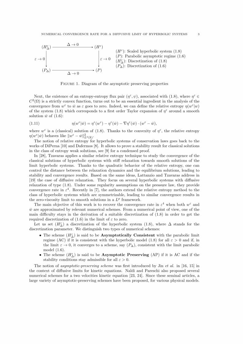
NUMERICAL CONVERGENCE RATE FOR A DIFFUSIVE LIMIT OF HYPERBOLIC SYSTEMS 3
(Hε∆) (Hε)
(P∆) (P )∆→ 0
ε→ 0 ε→ 0
∆→ 0
(Hε): Scaled hyperbolic system (1.8)(P ): Parabolic asymptotic regime (1.6)(Hε
∆): Discretization of (1.8)(P∆): Discretization of (1.6)
Figure 1. Diagram of the asymptotic preserving properties
Next, the existence of an entropy-entropy flux pair (ηε, ψ), associated with (1.8), where ηε ∈C2(Ω) is a strictly convex function, turns out to be an essential ingredient in the analysis of theconvergence from wε to w as ε goes to zero. Indeed, we can define the relative entropy η(wε|w)of the system (1.8) which corresponds to a first order Taylor expansion of ηε around a smoothsolution w of (1.6):
(1.11) η(wε|w) = ηε(wε)− ηε(w)−∇ηε(w) · (wε − w),
where wε is a (classical) solution of (1.8). Thanks to the convexity of ηε, the relative entropyη(wε|w) behaves like ‖wε − w‖2L2(R).
The notion of relative entropy for hyperbolic systems of conservation laws goes back to theworks of DiPerna [10] and Dafermos [8]. It allows to prove a stability result for classical solutionsin the class of entropy weak solutions, see [9] for a condensed proof.
In [28], Tzavaras applies a similar relative entropy technique to study the convergence of theclassical solutions of hyperbolic systems with stiff relaxation towards smooth solutions of thelimit hyperbolic systems. Thanks to the quadratic behavior of the relative entropy, one cancontrol the distance between the relaxation dynamics and the equilibrium solutions, leading tostability and convergence results. Based on the same ideas, Lattanzio and Tzavaras address in[19] the case of diffusive relaxation. They focus on several hyperbolic systems with diffusiverelaxation of type (1.8). Under some regularity assumptions on the pressure law, they provideconvergence rate in ε4. Recently in [7], the authors extend the relative entropy method to theclass of hyperbolic systems which are symmetrizable, leading to similar convergence results inthe zero-viscosity limit to smooth solutions in a Lp framework.
The main objective of this work is to recover the convergence rate in ε4 when both wε andw are approximated by relevant numerical schemes. From a numerical point of view, one of themain difficulty stays in the derivation of a suitable discretization of (1.8) in order to get therequired discretization of (1.6) in the limit of ε to zero.
Let us set (Hε∆) a discretization of the hyperbolic system (1.8), where ∆ stands for the
discretization parameter. We distinguish two types of numerical schemes:
• The scheme (Hε∆) is said to be Asymptotically Consistent with the parabolic limit
regime (AC) if it is consistent with the hyperbolic model (1.8) for all ε > 0 and if, inthe limit ε → 0, it converges to a scheme, say (P∆), consistent with the limit parabolicmodel (1.6).
• The scheme (Hε∆) is said to be Asymptotic Preserving (AP) if it is AC and if the
stability conditions stay admissible for all ε > 0.
The notion of asymptotic-preserving scheme was first introduced by Jin et al. in [16, 15] inthe context of diffusive limits for kinetic equations. Naldi and Pareschi also proposed severalnumerical schemes for a two velocities kinetic equation [23, 24]. Since these seminal articles, alarge variety of asymptotic-preserving schemes have been proposed, for various physical models.
4 C. BERTHON, M. BESSEMOULIN-CHATARD, AND H. MATHIS
Concerning specifically the discretization of hyperbolic systems with source terms in the diffusivelimit, Gosse and Toscani proposed a well-balanced and asymptotic-preserving scheme for theGoldstein-Taylor model in [11], and then for more general discrete kinetic models in [12]. In [1],Berthon and Turpault propose a modification of the HLL scheme [13] for hyperbolic systems toinclude source terms, and then a correction which allows to be consistent at the diffusive limit.More recently, several works are devoted to the derivation of asymptotic-preserving schemes for2D problems on unstructured meshes [3, 4, 5].
The purpose of this article is to study the convergence rate of the numerical scheme (Hε∆)
towards the numerical scheme (P∆) as ε tends to 0 (see Figure 1). After the work by Lattanzioand Tzavaras [19], we here adopt an error estimation given by a relative entropy in order toexhibit the required convergence rate from (Hε
∆) to (P∆). Indeed, in [19], the relative entropyis considered to establish the expected convergence rate from the scaled p-system (1.8) to theporous media problem (1.6). Let us note that the relative entropies have been recently suggestedin [17, 6] in order to derive suitable error estimates for finite volume approximations of smoothsolutions of nonlinear hyperbolic systems.
The paper is organized as follows. In the next section, for the sake of completeness, we give themain properties satisfied by the relative entropy associated with (1.8). More precisely, we detailthe convergence rate obtained by Lattanzio and Tzavaras [19], from the so-called p-system (1.8)to the porous media equation (1.6). In fact, the establishment of this result is constructive andit will be suitably adapted to get the expected numerical convergence rate. Section 3 concernsour main result. By adopting a semi-discrete in space numerical scheme to approximate theweak solutions of (1.8), we exhibit the convergence rate as ε goes to zero, to recover a semi-discrete approximation of the porous media equation (1.6). Moreover, the obtained convergencerate, from a numerical point of view, exactly coincides with the one established in [19] from acontinuous point of view. The numerical convergence rate is next illustrated, in the last section,performing several numerical experiments by adopting a full discrete scheme proposed by Jin etal. [16]. The performed simulations give an approximated convergence rate in perfect agreementwith the numerical convergence rate established in Section 3. As a consequence, it seems thatour main result is thus optimal.
2. Convergence in the diffusive limit
In this section, we recall the convergence result established in [19] since it is useful in theforthcoming numerical development. For the sake of simplicity, the convergence statement isgiven by arguing smooth solutions. Such an assumption is not at all restrictive in the derivationof our main numerical result established in the next section. We refer to [19] to extend thefollowing results with weak solutions.
To exhibit the rate of convergence from (τε, uε), solution of (1.8), to (τ , u), solution of (1.6),in the limit of ε to zero, Lattanzio and Tzavaras [19] adopt the well-known relative entropy todefine an error estimate. Considering the p-system (1.8), the relative entropy is defined by
ηε(τ, u|τ , u) = ηε(τ, u)− ηε(τ , u)−∇ηε(τ , u) ·(τ − τu− u
),
=ε2
2(u− u)2 − P (τ |τ),(2.1)
with
(2.2) P (τ |τ) = P (τ)− P (τ)− p(τ)(τ − τ).
This relative entropy satisfies an evolution law given in the following statement.
NUMERICAL CONVERGENCE RATE FOR A DIFFUSIVE LIMIT OF HYPERBOLIC SYSTEMS 5
Lemma 2.1. Let (τε, uε) be a strong entropy solution of (1.8) and (τ , u) be a smooth solutionof (1.6). Then the relative entropy ηε, defined by (2.1), satisfies the following evolution law:
∂tηε(τε, uε|τ , u)+∂xψ(τε, uε|τ , u) =
− σ(uε − u)2 +1
σp(τε|τ)∂xxp(τ) +
ε2
σ(uε − u)∂xtp(τ),(2.3)
where
ψ(τ, u|τ , u) = (u− u)(p(τ)− p(τ)),(2.4)
p(τ |τ) = p(τ)− p(τ)− p′(τ)(τ − τ).(2.5)
Let us emphasize that equality (2.3) becomes an inequality as soon as the smoothness ofsolution (τε, uε) is lost. The numerical counterpart is fully proved in the next section.
Proof. First, let us rewrite the parabolic system (1.6) such that we get the same left hand sidethan for the scaled p-system (1.8). Then, (1.6) reads equivalently as follows:
(2.6)
∂tτ − ∂xu = 0,
ε2∂tu+ ∂xp(τ) = −σ u+ ε2∂tu.
As a consequence, the derivative with respect to time of the relative entropy (2.1) satisfies thefollowing sequence of equalities:
∂tηε(τε, uε|τ , u) = ε2(uε − u)∂t(u
ε − u)− p(τε)∂tτε + p(τ)∂tτ
+ p′(τ)∂tτ(τε − τ) + p(τ)∂t(τε − τ)
= −(uε − u)∂x (p(τε)− p(τ))− σ(uε − u)2 − ε2(uε − u)∂tu
− p(τε)∂xuε + p′(τ)(τε − τ)∂xu+ p(τ)∂xuε,
= −σ(uε − u)2 +ε2
σ(uε − u)∂xtp(τ)
− ∂x(
(p(τε)− p(τ)) (uε − u))− p(τε|τ)∂xu.
The expected result directly comes from −σu = ∂xu to write ∂xu = − 1σ∂xxp(τ). The proof is
thus completed.
From now on, let us establish a technical result satisfied by the relative internal energy P (τ |τ),defined by (2.2).
Lemma 2.2. Assume that the pressure function p(τ) satisfies the conditions (1.2). Then thereexists two positive constants, C and C ′, such that for all τ ≥ c > 0 and τ ≥ c > 0, we have
(2.7) |p(τ |τ)| ≤ C ′(τ − τ)2 ≤ −C P (τ |τ).
where P (τ |τ) and p(τ |τ) are respectively defined by (2.2) and (2.5).
Proof. Since p belongs to C2(R∗+), by definition of p(τ |τ) and P (τ |τ), we immediately get
p(τ |τ) = (τ − τ)2
∫ 1
0
(1− s)p′′ (τ + s(τ − τ)) ds,
P (τ |τ) = (τ − τ)2
∫ 1
0
(1− s)p′ (τ + s(τ − τ)) ds.
Because of the smoothness of p, there exists a positive constant C ′ such that |p′′(τ +s(τ − τ))| ≤2C ′ for all s ∈ (0, 1). As a consequence, we obtain
|p(τ |τ)| ≤ C ′(τ − τ)2.
6 C. BERTHON, M. BESSEMOULIN-CHATARD, AND H. MATHIS
Moreover, the condition (1.2) imposes the existence of a positive constant m such that p′(τ +s(τ − τ)) ≤ −2m for all s ∈ (0, 1). Then we have
−P (τ |τ) ≥ m(τ − τ)2.
By considering C = C ′/m, the proof is achieved.
Arguing with these properties satisfied by the relative entropy, we are now able to compare(τε, uε), solution of (1.8), with (τ , u), solution of (1.6). To address such an issue and accordingto the assumptions stated in [19] (see also [25]), we impose that the porous media equation isgiven for admissible specific volumes τ ≥ c > 0. Moreover, the solutions of (1.6) are assumed tobe smooth, hence we can consider regularity on the pressure function (x, t) 7→ p(τ(x, t)) and itsderivatives.
In addition, we suppose that the systems (1.8) and (1.6) are endowed with initial conditionssuch that the following limits hold:
(2.8)lim
x→±∞τε(x, t) = lim
x→±∞τ(x, t) = τ±,
limx→±∞
uε(x, t) = limx→±∞
u(x, t) = 0,
where τ± are positive constant specific volume.Now, let us introduce the positive error estimate given by
(2.9) φε(t) =
∫Rηε(τε, uε|τ , u)dx,
to establish the expected convergence rate away from vanishing specific volume (see also [19]).
Theorem 2.3. Consider initial data (τ0(x), u0(x)) for (1.6) and (τε0 (x), uε0(x)) for (1.8) suchthat φε(0) < +∞. Endowed with these initial data, let (τ , u) be the smooth solution of (1.6)defined on QT = R× [0, T ), and let (τε, uε) be a strong entropy solution of (1.8). Let us assumethat τ ≥ c > 0. Moreover, let us assume that there exists a positive constant K such that‖∂xxp(τ)‖L∞(QT ) ≤ K and ‖∂xtp(τ)‖L2(QT ) ≤ K. Then the following stability estimate holds:
(2.10) φε(t) ≤ CeCT (φε(0) + ε4), t ∈ [0, T ),
where C is a constant depending on σ and p(τ). Moreover, if φε(0)→ 0 as ε→ 0, then
(2.11) supt∈[0,T )
φε(t)→ 0, as ε→ 0.
Proof. Arguing the limit assumptions (2.8), we have ψε(τε, uε|τ , u) → 0 in the limit x → ±∞.As a consequence, the integration of (2.3) over R× [0, t], for all t < T , gives
(2.12)
φε(t)− φε(0) ≤ −σ∫ t
0
∫R
(uε − u)2dx ds+1
σ
∫ t
0
∫R∂xxp(τ) p(τε|τ)dx ds
+ε2
σ
∫ t
0
∫R∂xtp(τ) (uε − u)dx ds.
Now, we estimate the integrals within the above relation. First, by Lemma 2.2 and since‖∂xxp(τ)‖L∞ ≤ K, there exists a positive constant, say C, such that we have
1
σ
∫ t
0
∫R|∂xxp(τ) p(τε|τ)|dx ds ≤ C
σ
∫ t
0
φε(s) ds.
NUMERICAL CONVERGENCE RATE FOR A DIFFUSIVE LIMIT OF HYPERBOLIC SYSTEMS 7
Concerning the last integral in (2.12), applying Cauchy-Schwarz and Young’s inequalitiestogether with the assumption on ‖∂xtp(τ)‖L2(QT ) ≤ K, we immediately obtain
ε2
σ
∫ t
0
∫R|∂xtp(τ) (uε − u)|dx ds ≤ σ
2
∫ t
0
∫R
(uε − u)2dx ds+ε4
2σ3
∫ t
0
∫R|∂xtp(τ)|2dx ds
≤ σ
2
∫ t
0
∫R
(uε − u)2dx ds+ C ε4.
As a consequence, identity (2.12) now reads
φε(t)− φε(0) ≤ −σ2
∫ t
0
∫R(uε − u)2dx ds+
C
σ
∫ t
0
φε(s) ds+ C ε4,
to get
φε(t) ≤ φε(0) +C
σ
∫ t
0
φε(s) ds+ C ε4.
The required estimation (2.10) is then obtained by the Gronwall’s inequality. The proof is thuscompleted.
3. Semi-discrete finite volume scheme and numerical convergence rate
In this section, our purpose concerns the evaluation of the convergence rate where both solu-tions wε and w are approximated by a semi-discrete scheme.
Let us consider a uniform mesh made of cells (xi− 12, xi+ 1
2)i∈Z of constant size ∆x. Here, the
discretization points are given by xi = i∆x for all i ∈ Z. On each cell (xi− 12, xi+ 1
2), the solutions
of (1.8) are approximated by time dependent piecewise constant function wi(t) = t(τi(t), ui(t)).For the sake of clarity in the notations, we omit the dependence on the parameter ε. Next, thesefunctions are evolved in time by adopting a semi-discrete scheme. Here, the suggested semi-discrete scheme is base on the standard HLL numerical flux (see [13]). Hence the semi-discretein space numerical scheme, to approximate the solutions of (1.8), reads
(3.1)
d
dtτi =
1
2∆x(ui+1 − ui−1) +
λ
2∆x(τi+1 − 2τi + τi−1),
d
dtui =
λ
2∆x(ui+1 − 2ui + ui−1)− 1
2ε2∆x(p(τi+1)− p(τi−1))− σ
ε2ui,
where we have set
(3.2) λ = supt∈(0,T )
maxi∈Z
(√−p′(τi)).
Let us underline that, as soon as ε goes to zero, the adopted semi-discrete finite volume schemeturns out to be consistent with the porous media equation (1.6) (AC according to the definitionstated in the introduction). As a consequence, the pair wi = t(τ i(t), ui(t)), to approximate thesolutions of (1.6), are evolved in time as follows:
(3.3)
d
dtτi =
1
2∆x(ui+1 − ui−1) +
λ
2 ∆x(τi+1 − 2τi + τi−1),
σui = −p(τi+1)− p(τi−1)
2∆x
We now analyze the convergence from (τi, ui) to (τ i, ui) as ε tends to zero. First, let us imposethe limit condition (2.8) to be imposed to the approximate solution as follows:
(3.4)
limi→±∞
τi = limi→±∞
τi = τ±,
limi→±∞
ui = limi→±∞
ui = 0.
8 C. BERTHON, M. BESSEMOULIN-CHATARD, AND H. MATHIS
Next, to simplify the forthcoming estimations, we introduce several semi-discrete norms. Letv(t) = (vi(t))i∈Z a function of time t ∈ [0, T ) piecewise constant on cells (xi− 1
2, xi+ 1
2). Then we
define
‖Dxv‖L∞(QT ) = supt∈[0,T )
supi∈Z
∣∣∣∣vi+1 − vi∆x
∣∣∣∣ ,‖Dxxv‖L∞(QT ) = sup
t∈[0,T )
supi∈Z
∣∣∣∣vi+2 − 2vi + vi−2
(2∆x)2
∣∣∣∣ ,(3.5)
‖Dxxv‖L∞(QT ) = supt∈[0,T )
supi∈Z
∣∣∣∣vi+1 − 2vi + vi−1
(∆x)2
∣∣∣∣ ,(3.6)
‖Dtxv‖L2(QT ) =
(∫ t
0
∑i∈Z
∆x
∣∣∣∣ ddt(vi+1 − vi−1
2∆x
)∣∣∣∣2 (s)ds
)1/2
,(3.7)
‖Dxxv‖L2(QT ) =
(∫ t
0
∑i∈Z
∆x
∣∣∣∣vi+1 − 2vi + vi−1
(∆x)2
∣∣∣∣2 (s)ds
)1/2
,(3.8)
where QT = R× [0, T ).We adopt the approach introduced by Lattanzio and Tzavaras [19] to the semi-discrete scheme
(3.1). As a first step, according to the definition of the relative entropy given by (2.1), we nowset
(3.9)
ηεi (t) = ηε(τi, ui|τi, ui)(t)
=ε2
2(ui(t)− ui(t))2 − P (τi(t)|τi(t)).
Mimicking the continuous framework, we introduce φε(t) to denote the discrete space integralof ηεi (t) as follows:
(3.10) φε(t) =∑i∈Z
∆x ηεi (t).
Without ambiguity and for the sake of clarity, the time dependence is omitted in the sequel.Now, we give our main result.
Theorem 3.1. Let wi(t) = (τi(t), ui(t))i∈Z be a smooth solution of (3.3) away from zero, definedon QT = R × [0, T ). We assume the existence of a positive constant K < +∞ such that thefollowing estimations are satisfied:
‖Dtxp(τ)‖L2(QT ) ≤ K, ‖Dxxp(τ)‖L∞(QT ) ≤ K(3.11)
‖Dxxτ‖L∞(QT ) ≤ K, ‖Dxτ‖L∞(QT ) ≤ K, ‖Dxxu‖L2(QT ) ≤ K.(3.12)
Let wi(t) = (τi(t), ui(t))i∈Z be a solution of (3.1), away from zero, such that φε(0) < +∞. Thenwe have
(3.13) φε(t) ≤ BeBT (φε(0) + ε4), t ∈ [0, T ),
where B is a positive constant which depends on K and σ. Moreover if φε(0)→ 0 as ε→ 0 thensupt∈[0,T ) φ
ε(t)→ 0 when ε→ 0.
Let us emphasize that the regularity conditions (3.11) exactly coincide with the smoothnessimposed in Theorem 2.3. Here, because of the numerical viscous terms, additional assumptions,stated in (3.12), must be imposed on the approximate solution of the porous media equation.However such conditions are not restrictive since solutions of the parabolic system (1.6), ingeneral, come with enough smoothness.
NUMERICAL CONVERGENCE RATE FOR A DIFFUSIVE LIMIT OF HYPERBOLIC SYSTEMS 9
Now, we turn to establish the above statement. To access such an issue, we need three technicalresults. The first one is devoted to exhibit the evolution law satisfied by the relative entropyηεi . We will see that this evolution law turns out to be a discrete form of (2.3) supplemented bynumerical viscosity. The two next Lemmas concern estimations of the numerical viscous termsassociated to the relative entropy.
Concerning the evolution law satisfied by ηεi , we have the following result:
Lemma 3.2. Let (τi, ui)i∈Z be a smooth solution of (3.3) and let (τi, ui)i∈Z be a solution of(3.1). The relative entropy ηεi , defined by (3.9), verifies the following evolution law:
(3.14)
dηεidt
+1
∆x(ψi+1/2 − ψi−1/2) = −σ(ui − ui)2
+1
σ
p(τi+2)− 2p(τi) + p(τi−2)
(2∆x)2p(τi|τi)
+ε2
σ(ui − ui)
d
dt
(p(τi+1)− p(τi−1)
2∆x
)+Rui +Rτi ,
where ψi+1/2 corresponds to an approximation of the relative entropy flux ψ at the interfacexi+1/2 given by
(3.15) ψi+1/2 =1
2(ui − ui)(p(τi+1)− p(τ i+1)) +
1
2(ui+1 − ui+1)(p(τi)− p(τi)),
and the quantities Rui and Rτi denote numerical residuals given by
(3.16)Rui =
λε2
2∆x(ui − ui)(ui+1 − 2ui + ui−1),
Rτi = − λ
2∆x
((p(τi)− p(τi))(τi+1 − 2τi + τi−1)− (τi − τi)p′(τi)(τi+1 − 2τi + τi−1)
).
From now on, we state estimations satisfied by both residuals Rui and Rτi .
Lemma 3.3. Let K < +∞ be a positive constant. Assume ‖Dxxu‖2L2(QT ) ≤ K, then for all
θ ∈ R∗+, we have
(3.17)
∫ t
0
∑i∈Z
∆x Rui ds ≤λθ
2
∫ t
0
∑i∈Z
∆x (ui − ui)2ds+ε4λ∆x
2θ‖Dxxu‖2L2(QT ).
Lemma 3.4. Let K < +∞ be a positive constant. Let us assume ‖Dxxτ‖L∞(QT ) ≤ K and‖Dxτ‖L∞(QT ) < K. Then there exists a positive constant C such that
(3.18)
∫ t
0
∑i∈Z
∆x Rτi ds ≤ λ(C ∆x‖Dxxτ‖L∞(QT ) + C‖Dxτ‖L∞(QT )
)∫ t
0
φε(s)ds.
Equipped with these three technical lemmas, we now establish our main result.
Proof of Theorem 3.1. Arguing Lemma 3.3, we evaluate the function φε by a discrete integrationin space of the equation (3.14) and next, an integration in time over [0, t). Since the limitassumptions (3.4) hold, the relative entropy flux tends to 0 when i→ ±∞. As a consequence, a
10 C. BERTHON, M. BESSEMOULIN-CHATARD, AND H. MATHIS
straightforward computation gives
(3.19)
φε(t)− φε(0) = −σ∫ t
0
∑i∈Z
∆x (ui − ui)2(s)ds
+1
σ
∫ t
0
∑i∈Z
∆x
(p(τi+2)− 2p(τi) + p(τi−2)
(2∆x)2p(τi|τi)
)(s)ds
+ε2
σ
∫ t
0
∑i∈Z
∆x
((ui − ui)
d
dt
(p(τi+1)− p(τi−1)
2∆x
))(s)ds
+
∫ t
0
∑i∈Z
∆x (Rui +Rτi )(s)ds.
Now, we evaluate each term involved within the right-hand side. Let us note that the second andthird terms of (3.19) are nothing but the discrete counterparts of the second and third terms in(2.12).
Concerning the second term of (3.19), from the definition (3.5) of ‖Dxxp(τ)‖L∞(QT ) andLemma 2.2, the following estimation holds:
1
σ
∫ t
0
∑i∈Z
∆x
∣∣∣∣p(τi+2)− 2p(τi) + p(τi−2)
(2∆x)2p(τi|τi)
∣∣∣∣(s)ds ≤− C
σ‖Dxxp(τ)‖L∞(QT )
∫ t
0
∑i∈Z
∆xP (τi|τ i)(s)ds.
Because of definition (3.9), we have −P (τi|τ i) ≤ ηεi . As a consequence, by definition of φε givenby (3.10), we immediately obtain
1
σ
∫ t
0
∑i∈Z
∆x
∣∣∣∣p(τi+2)− 2p(τi) + p(τi−2)
(2∆x)2p(τi|τi)
∣∣∣∣ (s)ds ≤ C
σ‖Dxxp(τ)‖L∞(QT )
∫ t
0
φε(s)ds.
(3.20)
Concerning the third term in (3.19), we use the Cauchy-Schwarz and Young’s inequalities toget
ε2
σ
∫ t
0
∑i∈Z
∆x
∣∣∣∣(ui − ui) ddt(p(τi+1)− p(τi−1)
2∆x(s)
)∣∣∣∣ ds≤ σ
2
∫ t
0
∑i∈Z
∆x |ui − ui|2(s)ds+ε4
2σ3
∫ t
0
∑i∈Z
∆x
∣∣∣∣ ddt(p(τi+1)− p(τi−1)
2∆x(s)
)∣∣∣∣2 ds.Involving the definition (3.7) of ‖Dtxp(τ)‖L2(QT ), the following estimation holds:
(3.21)
ε2
σ
∫ t
0
∑i∈Z
∆x
∣∣∣∣(ui − ui) ddt(p(τi+1)− p(τi−1)
2∆x
)∣∣∣∣ (s)ds≤ σ
2
∫ t
0
∑i∈Z
∆x (ui − ui)2ds+ε4
2σ3‖Dtxp(τ)‖2L2(QT ).
Now, the control of the numerical error terms Rui and Rτi is established in Lemma 3.3 andLemma 3.4, in order to have the estimations of the last term in (3.19). Accounting on the
NUMERICAL CONVERGENCE RATE FOR A DIFFUSIVE LIMIT OF HYPERBOLIC SYSTEMS 11
estimations (3.17), (3.18), (3.20) and (3.21), from the relation (3.19) we write(3.22)
φε(t) ≤ φε(0) +
(λθ
2− σ
2
)∫ t
0
∑i∈Z
∆x (ui − ui)2(s)ds
+
(1
2σ3‖Dtxp(τ)‖2L2(QT ) +
λ∆x
2θ‖Dxxu‖2L2(QT )
)ε4
+
(Cλ∆x‖Dxxτ‖L∞(QT ) + Cλ‖Dxτ‖L∞(QT ) +
C
σ‖Dxxp(τ)‖L∞(QT )
)∫ t
0
φε(s)ds.
Let us fix θ ≤ σ
λsuch that
λθ
2− σ
2≤ 0. Then we get
(3.23)
φε(t) ≤ φε(0) +
(1
2σ3‖Dtxp(τ)‖2L2(QT ) +
λ∆x
2θ‖Dxxu‖2L2(QT )
)ε4
+
(C
σ‖Dxxp(τ)‖L∞(QT ) + λC ∆x‖Dxxτ‖L∞(QT ) +
λC
2‖Dxτ‖L∞(QT )
)∫ t
0
φε(s)ds.
The expected estimation (3.13) is a direct consequence of the Gronwall Lemma. The proof isthus completed.
To conclude this section, we now give the proofs of the three intermediate results.
Proof of Lemma 3.2. From (3.9), the derivative with respect to time of the relative entropy ηεireads
(3.24)d
dtηεi = ε2(ui − ui)
d
dt(ui − ui)− (p(τi)− p(τi))
d
dtτi + (τi − τi)p′(τi)
d
dtτi.
Now, let us rewrite the second equation of (3.3) as follows:
(3.25) ε2 d
dtui = ε2 d
dtui − σui −
1
2∆x(p(τi+1)− p(τi−1)).
From (3.1), since we have
ε2 d
dtui =
λε2
2∆x(ui+1 − 2ui + ui−1)− 1
2∆x(p(τi+1)− p(τi−1))− σui,
we obtain
ε2 d
dt(ui − ui) =− σ(ui − ui)− ε2 d
dtui −
1
2∆x
((p(τi+1)− p(τi−1))− (p(τi+1)− p(τi−1))
)+
λε2
2∆x(ui+1 − 2ui + ui−1).
Plugging the above relation into (3.24) leads to
(3.26)
d
dtηεi =− σ(ui − ui)2 − ε2(ui − ui)
d
dtui
− (ui − ui)1
2∆x
((p(τi+1)− p(τi−1))− (p(τi+1)− p(τi−1))
)+
λε2
2∆x(ui − ui)(ui+1 − 2ui + ui−1)
− (p(τi)− p(τi))d
dtτi + (τi − τi)p′(τi)
d
dtτi.
12 C. BERTHON, M. BESSEMOULIN-CHATARD, AND H. MATHIS
Next, we substituted
dtτi and
d
dtτi by their definitions, given by (3.1) and (3.3), to obtain
(3.27)
d
dtηεi =− σ(ui − ui)2 − ε2(ui − ui)
d
dtui
− 1
2∆x
(p(τi+1)− p(τ i+1))(ui − ui)− (p(τi−1)− p(τi−1))(ui − ui)
+ (p(τi)− p(τi))(ui+1 − ui−1)− (τi − τi)p′(τi)(ui+1 − ui−1))
+λε2
2∆x(ui − ui)(ui+1 − 2ui − ui−1)
− λ
2∆x
((p(τi)− p(τi))(τi+1 − 2τi + τi−1)− (τi − τi)p′(τi)(τi+1 − 2τi + τi−1)
),
Let us remark that the two last terms are respectively the numerical error terms Rui and Rτidefined in (3.16). Moreover, by definition of p(τi|τi), given by (2.5), the above relation rewritesas follows:
(3.28)
d
dtηεi =− σ(ui − ui)2 − ε2(ui − ui)
d
dtui
− 1
2∆x
((ui+1 − ui−1)p(τi|τi) + (ui − ui)(p(τi+1)− p(τi+1))
+ (p(τi)− p(τi))(ui+1 − ui+1)− (ui−1 − ui−1)(p(τi)− p(τi))
− (ui − ui)(p(τi−1)− p(τi−1)))
+Rui +Rτi ,
Adopting the definition (3.15) of the discrete relative entropy flux ψi+1/2, we directly obtain
(3.29)
d
dtηεi =− σ(ui − ui)2 − ε2(ui − ui)
d
dtui
− 1
∆x(ψi+1/2 − ψi−1/2)
− 1
2∆x(ui+1 − ui−1)p(τi|τi)
+Rui +Rτi .
Finally, from the scheme definition (3.3), we deduce the following two relations:
d
dtui = − 1
2σ∆x
d
dt(p(τi+1)− p(τi−1)),
ui+1 − ui−1 = − 1
2σ∆x(p(τi+2)− 2p(τi) + p(τi−2)) ,
to recover the expected evolution law (3.14). The proof is thus achieved.
Proof of Lemma 3.3. Because of the definition (3.16) of the residual Rui , we have
(3.30)
∫ t
0
∑i∈Z
∆x Rui (s)ds =ε2λ
2
∫ t
0
∑i∈Z
(ui+1 − 2ui + ui−1)(ui − ui)(s)ds,
NUMERICAL CONVERGENCE RATE FOR A DIFFUSIVE LIMIT OF HYPERBOLIC SYSTEMS 13
which equivalently rewrites as follows:(3.31)∫ t
0
∑i∈Z
∆x Rui (s)ds =ε2λ
2
∫ t
0
∑i∈Z
(ui+1 − 2ui + ui−1
)(ui − ui)(s)ds
+ε2λ
2
∫ t
0
∑i∈Z
((ui+1 − ui+1)− 2(ui − ui) + (ui−1 − ui−1))
)(ui − ui)(s)ds.
Since ui and ui satisfy the assumption limit (3.4), we immediately have∑i∈Z
((ui+1 − ui+1)− 2(ui − ui) + (ui−1 − ui−1))
)(ui − ui) =
−∑i∈Z
((ui+1 − ui+1)− (ui − ui)
)2
.
As a consequence, we obtain the following inequality:∫ t
0
∑i∈Z
∆x Rui (s)ds ≤ ε2λ
2
∫ t
0
∑i∈Z
(ui+1 − 2ui + ui−1
)(ui − ui)(s)ds,
which rewrites
(3.32)
∫ t
0
∑i∈Z
∆x Rui (s)ds ≤ ε2λ∆x
2
∫ t
0
∑i∈Z
√∆x
ui+1 − 2ui + ui−1
(∆x)2
√∆x(ui − ui)ds.
Combining again Cauchy-Schwarz and Young’s inequalities gives, for all θ > 0,
(3.33)
∫ t
0
∑i∈Z
∆x Rui (s)ds ≤ ε4λ∆x
2θ
∫ t
0
∑i∈Z
∆x
(ui+1 − 2ui + ui−1
(∆x)2
)2
ds
+λθ
2
∫ t
0
∑i∈Z
∆x (ui − ui)2ds.
Finally, the definition (3.8) of ‖Dxxu‖L2(QT ) leads to the required inequality (3.17).
Proof of Lemma 3.4. First, arguing the definition of p(τi|τi), given by (2.5), a straightforwardcomputation leads to the following reformulation of Rτi :
(3.34)Rτi =− λ
2∆x
(p(τi|τi)(τi+1 − 2τi + τi−1)
)+
λ
2∆x
((p(τi)− p(τi)) ((τi+1 − τi+1)− 2(τi − τi) + (τi−1 − τi−1))
),
to get
(3.35)
∫ t
0
∑i∈Z
∆x Rτi ds = T1 + T2,
where we have set
T1 = −λ2
∫ t
0
∑i∈Z
p(τi|τi)(τi+1 − 2τi + τi−1)ds,(3.36)
T2 = −λ2
∫ t
0
∑i∈Z
(p(τi)− p(τi))(
(τi+1 − τi+1)− 2(τi − τi) + (τi−1 − τi−1))ds.(3.37)

14 C. BERTHON, M. BESSEMOULIN-CHATARD, AND H. MATHIS
We first estimate T1. Thanks to Lemma 2.2, we write
(3.38) T1 ≤ −∆xλC
2
∫ t
0
∑i∈Z
∆x P (τi|τi)∣∣∣∣ τi+1 − 2τi + τi−1
(∆x)2
∣∣∣∣ ds.Since we have −P (τi|τ i) ≤ ηεi and ‖Dxxτ‖L∞(QT ) is bounded, we easily obtain
(3.39) T1 ≤ ∆xλC‖Dxxτ‖L∞(QT )
∫ t
0
φε(s)ds.
Now, let focus on T2. By a discrete integration by parts, we directly get
T2 =λ
2
∫ t
0
∑i∈Z
((p(τi+1)− p(τi+1))− (p(τi)− p(τi))
)((τi+1 − τi+1)− (τi − τi)
),
to write
T2 =λ
2
∫ t
0
∑i∈Z
(p(τi+1)− p(τi))(
(τi+1 − τi+1)− (τi − τi))
− λ
2
∫ t
0
∑i∈Z
(p(τi+1)− p(τi))(
(τi+1 − τi+1)− (τi − τi)).
With some abuse in the notations, we introduce
p(τi+1)− p(τi)τi+1 − τi
(τi+1 − τi) =
p(τi+1)− p(τi) if τi+1 − τi 6= 0,0 otherwise,
to rewrite T2 as follows:
(3.40)
T2 =λ
2
∫ t
0
∑i∈Z
p(τi+1)− p(τi)τi+1 − τi
((τi+1 − τi+1)− (τi − τi)
)(τi+1 − τi)ds
− λ
2
∫ t
0
∑i∈Z
p(τi+1)− p(τi)τi+1 − τi
((τi+1 − τi+1)− (τi − τi)
)(τi+1 − τi)ds.
We notice that((τi+1 − τi+1)− (τi − τi)
)(τi+1 − τi) =
((τi+1 − τi+1)− (τi − τi)
)2
+ (τi+1 − τi)(
(τi+1 − τi+1)− (τi − τi)),
so that T2 now reads
(3.41)
T2 =λ
2
∫ t
0
∑i∈Z
p(τi+1)− p(τi)τi+1 − τi
((τi+1 − τi+1)− (τi − τi)
)2
ds
+λ
2
∫ t
0
∑i∈Z
p(τi+1)− p(τi)τi+1 − τi
(τi+1 − τi)(
(τi+1 − τi+1)− (τi − τi))
− λ
2
∫ t
0
∑i∈Z
p(τi+1)− p(τi)τi+1 − τi
((τi+1 − τi+1)− (τi − τi)
)(τi+1 − τi)ds.
According to the assumption (1.2), the pressure p is a decreasing function of τ . As a consequence,the first term of (3.41) is nonpositive. Hence we obtain
(3.42) T2 ≤λ
2
∫ t
0
∑i∈Z
(p(τi+1)− p(τi)τi+1 − τi
− p(τi+1)− p(τi)τi+1 − τi
)((τi+1−τi+1)−(τi−τi)
)(τi+1−τi)ds.
NUMERICAL CONVERGENCE RATE FOR A DIFFUSIVE LIMIT OF HYPERBOLIC SYSTEMS 15
Under the assumption (3.12) on ‖Dxτ‖L∞(QT ), the above relation becomes
(3.43)T2 ≤
λ
2‖Dxτ‖L∞(QT )
∫ t
0
∑i∈Z
∆x
∣∣∣∣p(τi+1)− p(τi)τi+1 − τi
− p(τi+1)− p(τi)τi+1 − τi
∣∣∣∣× |(τi+1 − τi+1)− (τi − τi)| ds.
Now, let us emphasize that we have∣∣∣∣p(τi+1)− p(τi)τi+1 − τi
− p(τi+1)− p(τi)τi+1 − τi
∣∣∣∣ ≤ ∫ 1
0
∣∣∣p′(τi + z(τi+1 − τi))− p′(τi + z(τi+1 − τi)))∣∣∣dz.
Since p ∈ C2(R∗+), the function p′ is Lipschitz continuous with a Lipschitz constant D. Then thefollowing sequence of inequalities holds:∣∣∣∣p(τi+1)− p(τi)
τi+1 − τi− p(τi+1)− p(τi)
τi+1 − τi
∣∣∣∣ ≤ D ∫ 1
0
∣∣∣(τi + z(τi+1 − τi))− (τi + z(τi+1 − τi)∣∣∣dz,
≤ D∫ 1
0
((1− z)|τi − τi|+ z|τi+1 − τi+1|
)dz,
≤ D
2(|τi − τi|+ |τi+1 − τi+1|) .
Plugging this estimation into (3.43) gives
T2 ≤λ
2
D
2‖Dxτ‖L∞(QT )
∫ t
0
∑i∈Z
∆x (|τi+1 − τi+1)|+ |τi − τi)|)2ds,
≤ λD‖Dxτ‖L∞(QT )
∫ t
0
∑i∈Z
∆x |τi − τi|2ds.
By Lemma 2.2, there exists a positive constant C such that |τi − τ i|2 ≤ −CP (τi|τ i) ≤ Cηεi . Asa consequence, there exists a constant, once again denoted C, such that we have
(3.44) T2 ≤ λC‖Dxτ‖L∞(QT )
∫ t
0
φε(s)ds,
Both inequalities (3.39) and (3.44) complete the estimation of Rτi and the proof is achieved.
4. Numerical illustrations
In this section, we perform numerical experiments to attest the relevance of the establishedconvergence rate given by (3.13). To address such an issue, we consider a fully discrete schemeas proposed by Jin et al. in [16]. This scheme is based on a reformulation of system (1.8) asfollows:
∂tτ − ∂xu = 0,
∂tu+ ∂xp(τ) = − 1
ε2
(σ u+ (1− ε2)∂xp(τ)
).
Arguing this reformulation, a 2-step splitting technique is adopted. During the first step, a purelyconvective and non-stiff system is considered:
∂tτ − ∂xu = 0,
∂tu+ ∂xp(τ) = 0.
16 C. BERTHON, M. BESSEMOULIN-CHATARD, AND H. MATHIS
Its solutions are approximated by adopting a classical HLL scheme [13]:
τn+ 1
2i = τni −
∆t
∆x
(Fτi+ 1
2−Fτi− 1
2
),(4.1a)
un+ 1
2i = uni −
∆t
∆x
(Fui+ 1
2−Fui− 1
2
),(4.1b)
where the numerical fluxes are defined by
Fτi+ 12
=1
2(−uni − uni+1)− λ
2(τni+1 − τni ),
Fui+ 12
=1
2(p(τni ) + p(τni+1))− λ
2(uni+1 − uni ).
It is well known that this scheme is stable under the CFL condition∆t
∆xλ ≤ 1
2, where λ is defined
by (3.2), which does not depend on ε. Next, the stiff source term is treated by a second stepwhere the following system is discretized:
∂tτ = 0,
∂tu = − 1
ε2
(σ u+ (1− ε2)∂xp(τ)
).
During this relaxation step, an implicit method is suggested in order to obtain unconditionalstability:
τn+1i = τ
n+ 12
i ,
un+1i − un+ 1
2i
∆t= − 1
ε2
σ un+1i + (1− ε2)
pn+1i+ 1
2
− pn+1i− 1
2
∆x
.
As in [16], the nodal values are given by the following centered discretization:
pn+1i+ 1
2
=1
2
(p(τn+1
i ) + p(τn+1i+1 )
).
Since τn+1i = τ
n+ 12
i , let us emphasize that un+1i can be computed explicitly from (τni , u
ni )i∈Z.
Finally, the relaxation step can be written as
τn+1i = τ
n+ 12
i ,(4.2a)
un+1i =
(ε2
ε2 + σ∆t
)un+ 1
2i −∆t
(1− ε2
∆t σ + ε2
)p(τ
n+ 12
i+1 )− p(τn+ 12
i−1 )
2 ∆x.(4.2b)
We underline that this scheme corresponds to the semi-discrete framework introduced Section 3.Indeed, combining (4.1b) and (4.2b), we get
un+1i = uni −
σ∆t
ε2 + σ∆tuni −
∆t
2 ∆x(ε2 + ∆t σ)
(p(τn+1
i+1 )− p(τn+1i−1 )
)+
∆t λ
2 ∆x
(ε2
ε2 + σ∆t
)(uni+1 − 2uni + uni−1).
Now, we fix ∆t =∆t ε2
ε2 + σ∆t, and we note that this new time increment is consistent with ∆t.
We immediately remark that we recover (3.1) as soon as ∆t tends to zero.

NUMERICAL CONVERGENCE RATE FOR A DIFFUSIVE LIMIT OF HYPERBOLIC SYSTEMS 17
Next, we consider the scheme (4.1)-(4.2) in the limit of ε to zero to approximate the solutionsof the parabolic problem (1.6). We get the following scheme:
τn+1i = τni +
∆t
2 ∆x
(uni+1 − uni−1
)− λ∆t
2 ∆x(τni+1 − 2τni + τni−1),
un+1i = − 1
2σ∆x
(p(τn+1
i+1 )− p(τn+1i−1 )
),
which is an approximation of (1.6).We notice that this scheme is AP in the sense of the definition given in the introduction.
Indeed, its limit as ε→ 0 is consistent (AC) with the parabolic problem (1.6), while its stabilitycondition does not depend on ε.
Equipped with this scheme, we now perform numerical experiments. We approximate thesolutions on the interval (−4, 4), and we consider zero-flux boundary conditions. The final timeof simulation is T = 10−2. The friction coefficient is fixed to σ = 1.
Concerning the pressure law, we adopt p(τ) = τ−γ where the adiabatic coefficient is fixed to1.4.
We compute the approximate solutions of the hyperbolic system (1.8) for different valuesof ε: 10−1, 3.10−2, 10−2, 3.10−3, 10−3, 3.10−4, 10−4, and different number of cells N =100, 200, 400, 1600. The two following initial data are considered:
• Condition 1 (discontinuous):
(4.3) τ0(x) =
2 if x < 0,1 if x > 0,
• Condition 2 (smooth):
(4.4) τ0(x) = exp(−100x2) + 1.
Here, the initial velocity u0 is computed to be compatible with the discrete diffusive limit inorder to avoid an initial layer:
u0i = − 1
σ
p(τ0i+1)− p(τ0
i−1)
2∆x.
We display, Figure 2, the discrete space integral of the relative entropy φε(T ) with respectto ε in log scale for the p-system. We observe that both for discontinuous and smooth initialcondition, and for different numbers of cells, the decay rate is always in O(ε4), which is in goodagreement with Theorem 3.1.
A natural extension of this work concerns the Goldstein-Taylor model, which reads
(4.5)
∂tρ
ε + ∂xjε = 0,
ε2∂tjε + ∂xρ
ε = −σ jε,(x, t) ∈ R× R+.
This system can be seen as a simplified two velocities kinetic model in macroscopic variables (seefor example [15, 24]). In the diffusion limit ε → 0, the Goldstein-Taylor model coincides withthe heat equation given by
(4.6)
∂tρ−1
σ∂xxρ = 0,
∂xρ = −σ j,(x, t) ∈ R× R+.
Concerning this model, a direct adaptation of the numerical scheme (4.1)-(4.2) is suggested. Thenumerical results are displayed Figure 3. As well as for the p-system case, the convergence rateis also in O(ε4) which is in good agreement with convergence results given in [19].
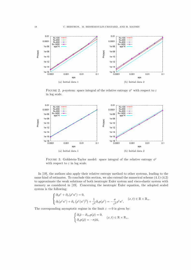
18 C. BERTHON, M. BESSEMOULIN-CHATARD, AND H. MATHIS
1e-16
1e-14
1e-12
1e-10
1e-08
1e-06
0.0001
0.01
0.0001 0.001 0.01 0.1
Ph
i(e
ps)
eps
N=100N=200N=400
N=1600eps^4
(a) Initial data 1
1e-16
1e-14
1e-12
1e-10
1e-08
1e-06
0.0001
0.01
0.0001 0.001 0.01 0.1
Ph
i(e
ps)
eps
N=100N=200N=400
N=1600eps^4
(b) Initial data 2
Figure 2. p-system: space integral of the relative entropy φε with respect to εin log scale.
1e-18
1e-16
1e-14
1e-12
1e-10
1e-08
1e-06
0.0001
0.01
0.0001 0.001 0.01 0.1
Ph
i(e
ps)
eps
N=100N=200N=400
N=1600eps^4
(a) Initial data 1
1e-18
1e-16
1e-14
1e-12
1e-10
1e-08
1e-06
0.0001
0.01
0.0001 0.001 0.01 0.1
Ph
i(e
ps)
eps
N=100N=200N=400
N=1600eps^4
(b) Initial data 2
Figure 3. Goldstein-Taylor model: space integral of the relative entropy φε
with respect to ε in log scale.
In [19], the authors also apply their relative entropy method to other systems, leading to thesame kind of estimates. To conclude this section, we also extend the numerical scheme (4.1)-(4.2)to approximate the weak solutions of both isentropic Euler system and visco-elastic system withmemory as considered in [19]. Concerning the isentropic Euler equation, the adopted scaledsystem is the following:
∂tρε + ∂x(ρεuε) = 0,
∂t(ρεuε) + ∂x
(ρε(uε)2
)+
1
ε2∂xp(ρ
ε) = − σε2ρεuε,
(x, t) ∈ R× R+.
The corresponding asymptotic regime in the limit ε→ 0 is given by:∂tρ− ∂xxp(ρ) = 0,
∂xp(ρ) = −σρu,(x, t) ∈ R× R+.
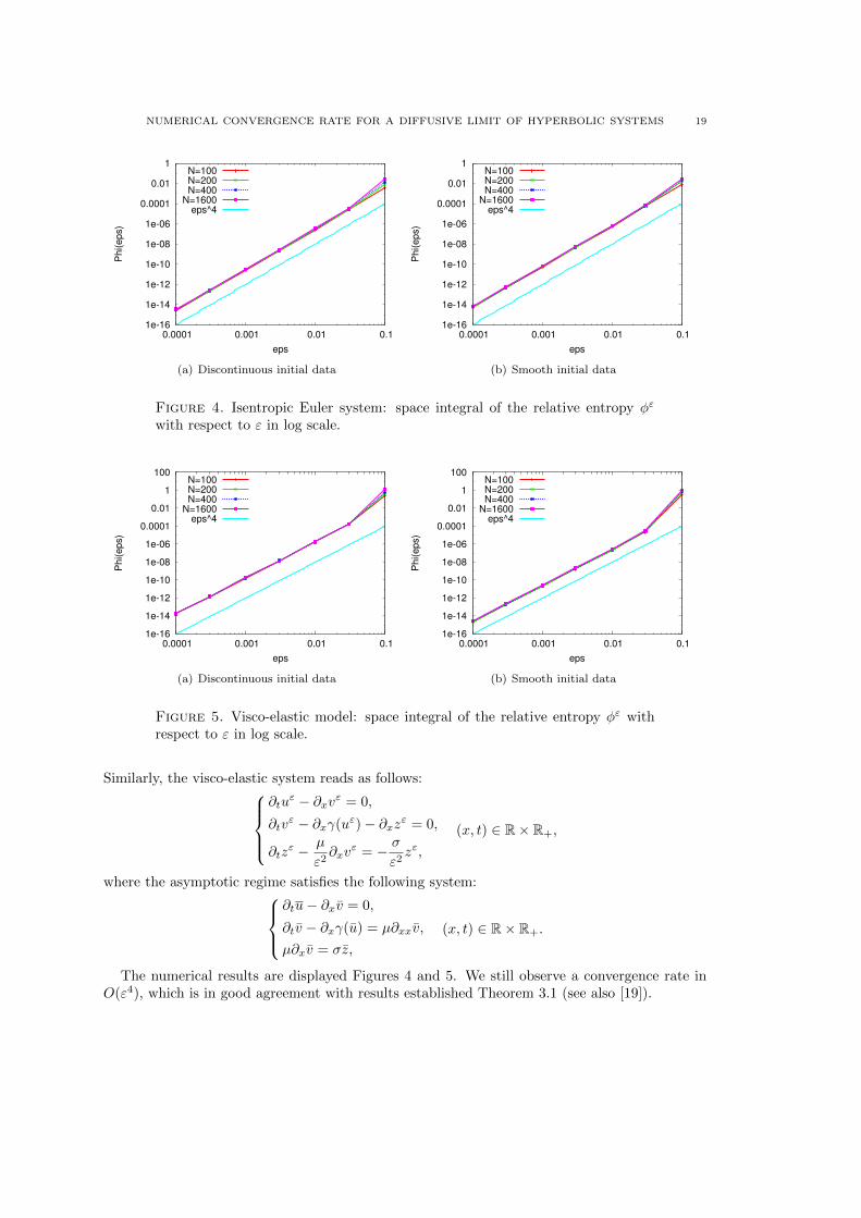
NUMERICAL CONVERGENCE RATE FOR A DIFFUSIVE LIMIT OF HYPERBOLIC SYSTEMS 19
1e-16
1e-14
1e-12
1e-10
1e-08
1e-06
0.0001
0.01
1
0.0001 0.001 0.01 0.1
Ph
i(e
ps)
eps
N=100N=200N=400
N=1600eps^4
(a) Discontinuous initial data
1e-16
1e-14
1e-12
1e-10
1e-08
1e-06
0.0001
0.01
1
0.0001 0.001 0.01 0.1
Ph
i(e
ps)
eps
N=100N=200N=400
N=1600eps^4
(b) Smooth initial data
Figure 4. Isentropic Euler system: space integral of the relative entropy φε
with respect to ε in log scale.
1e-16
1e-14
1e-12
1e-10
1e-08
1e-06
0.0001
0.01
1
100
0.0001 0.001 0.01 0.1
Ph
i(e
ps)
eps
N=100N=200N=400
N=1600eps^4
(a) Discontinuous initial data
1e-16
1e-14
1e-12
1e-10
1e-08
1e-06
0.0001
0.01
1
100
0.0001 0.001 0.01 0.1
Ph
i(e
ps)
eps
N=100N=200N=400
N=1600eps^4
(b) Smooth initial data
Figure 5. Visco-elastic model: space integral of the relative entropy φε withrespect to ε in log scale.
Similarly, the visco-elastic system reads as follows:∂tu
ε − ∂xvε = 0,
∂tvε − ∂xγ(uε)− ∂xzε = 0,
∂tzε − µ
ε2∂xv
ε = − σε2zε,
(x, t) ∈ R× R+,
where the asymptotic regime satisfies the following system:∂tu− ∂xv = 0,
∂tv − ∂xγ(u) = µ∂xxv,
µ∂xv = σz,
(x, t) ∈ R× R+.
The numerical results are displayed Figures 4 and 5. We still observe a convergence rate inO(ε4), which is in good agreement with results established Theorem 3.1 (see also [19]).
20 C. BERTHON, M. BESSEMOULIN-CHATARD, AND H. MATHIS
Acknowledgements. The authors thank the project ANR-12-IS01-0004 GeoNum and theproject ANR-14-CE25-0001 Achylles for their partial financial contributions.
References
[1] C. Berthon and R. Turpault. Asymptotic preserving HLL schemes. Numer. Methods Partial Differential
Equations, 27:1396–1422, 2011.[2] S. Bianchini, B. Hanouzet, and R. Natalini. Asymptotic behavior of smooth solutions for partially dissipative
hyperbolic systems with a convex entropy. Comm. Pure Appl. Math., 60(11):1559–1622, 2007.
[3] F. Blachere and R. Turpault. An admissibility and asymptotic-preserving scheme for systems of conservationlaws with source term on 2D unstructured meshes. Journal of Computational Physics, 2016.
[4] C. Buet, B. Despres, and E. Franck. Design of asymptotic preserving finite volume schemes for the hyperbolic
heat equation on unstructured meshes. Numerische Mathematik, 122(2):227–278, 2012.[5] C. Buet, B. Despres, E. Franck, and T. Leroy. Proof of uniform convergence for a cell-centered AP discretiza-
tion of the hyperbolic heat equation on general meshes. Math. of Comp., 2016.[6] C. Cances, H. Mathis, and N. Seguin. Relative entropy for the finite volume approximation of strong solutions
to systems of conservation laws. Submitted.
[7] C. Christoforou and A. Tzavaras. Relative entropy for hyperbolic-parabolic systems and application to theconstitutive theory of thermoviscoelasticity. ArXiv e-prints, March 2016.
[8] C. M. Dafermos. The second law of thermodynamics and stability. Arch. Rational Mech. Anal., 70(2):167–179,
1979.[9] C. M. Dafermos. Hyperbolic conservation laws in continuum physics, volume 325 of Grundlehren der Mathe-
matischen Wissenschaften [Fundamental Principles of Mathematical Sciences]. Springer-Verlag, Berlin, third
edition, 2010.[10] R. J. DiPerna. Uniqueness of solutions to hyperbolic conservation laws. Indiana Univ. Math. J., 28(1):137–
188, 1979.
[11] L. Gosse and G. Toscani. An asymptotic-preserving well-balanced scheme for the hyperbolic heat equations.C. R. Math. Acad. Sci. Paris, 334(4):337 – 342, 2002.
[12] L. Gosse and G. Toscani. Space localization and well-balanced schemes for discrete kinetic models in diffusiveregimes. SIAM J. Numer. Anal., 41(2):641–658 (electronic), 2003.
[13] A. Harten, P. D. Lax, and B. van Leer. On upstream differencing and Godunov-type schemes for hyperbolic
conservation laws. SIAM Rev., 25(1):35–61, 1983.[14] L. Hsiao and T.-P. Liu. Convergence to nonlinear diffusion waves for solutions of a system of hyperbolic
conservation laws with damping. Comm. Math. Phys., 143(3):599–605, 1992.
[15] S. Jin. Efficient asymptotic-preserving (AP) schemes for some multiscale kinetic equations. SIAM J. Sci.Comput., 21(2):441–454 (electronic), 1999.
[16] S. Jin, L. Pareschi, and G. Toscani. Diffusive relaxation schemes for multiscale discrete-velocity kinetic
equations. SIAM J. Numer. Anal., 35(6):2405–2439, 1998.[17] V. Jovanovic and C. Rohde. Error estimates for finite volume approximations of classical solutions for non-
linear systems of hyperbolic balance laws. SIAM J. Numer. Anal., 43(6):2423–2449 (electronic), 2006.[18] Shuichi Kawashima. Large-time behaviour of solutions to hyperbolic-parabolic systems of conservation laws
and applications. Proc. Roy. Soc. Edinburgh Sect. A, 106(1-2):169–194, 1987.
[19] C. Lattanzio and A.E. Tzavaras. Relative entropy in diffusive relaxation. SIAM J. Math. Anal., 45(3):1563–1584, 2013.
[20] P.L. Lions and G. Toscani. Diffusive limit for finite velocity Boltzmann kinetic models. Revista Matematica
Iberoamericana, 13(3):473–514, 1997.[21] P. Marcati, A.J. Milani, and P. Secchi. Singular convergence of weak solutions for a quasilinear nonhomoge-
neous hyperbolic system. Manuscripta Math., 60(1):49–69, 1988.[22] M. Mei. Best asymptotic profile for hyperbolic p-system with damping. SIAM J. Math. Anal., 42(1):1–23,
2010.
[23] G. Naldi and L. Pareschi. Numerical schemes for kinetic equations in diffusive regimes. Appl. Math. Lett.,
11(2):29–35, 1998.[24] G. Naldi and L. Pareschi. Numerical schemes for hyperbolic systems of conservation laws with stiff diffusive
relaxation. SIAM J. Numer. Anal., 37(4):1246–1270, 2000.[25] K. Nishihara. Convergence rates to nonlinear diffusion waves for solutions of system of hyperbolic conservation
laws with damping. J. Differential Equations, 131(2):171 – 188, 1996.
[26] K. Nishihara. Asymptotic behavior of solutions of quasilinear hyperbolic equations with linear damping. J.
Differential Equations, 137(2):384–395, 1997.

NUMERICAL CONVERGENCE RATE FOR A DIFFUSIVE LIMIT OF HYPERBOLIC SYSTEMS 21
[27] K. Nishihara, W. Wang, and T. Yang. Lp-convergence rate to nonlinear diffusion waves for p-system withdamping. J. Differential Equations, 161(1):191–218, 2000.
[28] A. E. Tzavaras. Relative entropy in hyperbolic relaxation. Commun. Math. Sci., 3(2):119–132, 2005.
[29] C. J. van Duyn and L. A. Peletier. A class of similarity solutions of the nonlinear diffusion equation. NonlinearAnal., 1(3):223–233, 1976/77.
[30] C. J. van Duyn and L. A. Peletier. Asymptotic behaviour of solutions of a nonlinear diffusion equation. Arch.
Ration. Mech. Anal., 65(4):363–377, 1977.
Universite de Nantes, Laboratoire de Mathematiques Jean Leray, CNRS UMR 6629, 2 rue de la
Houssiniere, BP 92208, 44322 Nantes, France
E-mail address: [email protected]
Universite de Nantes, Laboratoire de Mathematiques Jean Leray, CNRS UMR 6629, 2 rue de la
Houssiniere, BP 92208, 44322 Nantes, FranceE-mail address: [email protected]
Universite de Nantes, Laboratoire de Mathematiques Jean Leray, CNRS UMR 6629, 2 rue de la
Houssiniere, BP 92208, 44322 Nantes, FranceE-mail address: [email protected]