numerical characterization of porous solids and ... · numerical characterization of porous solids...

Copyright © 2010 Tech Science Press CMES, vol.55, no.1, pp.33-60, 2010

Numerical Characterization of Porous Solids andPerformance Evaluation of Theoretical Models via the

Precorrected-FFT Accelerated BEM

Z. Y. Yan1,2, J. Zhang1, W. Ye1 and T.X. Yu1

Abstract: An 3-D precorrected-FFT accelerated BEM approach for the linearelastic analysis of porous solids with randomly distributed pores of arbitrary shapeand size is described in this paper. Both the upper bound and the lower boundof elastic properties of solids with spherical pores are obtained using the devel-oped fast BEM code. Effects of porosity and pore shape on the elastic propertiesare investigated. The performance of several theoretical models is evaluated bycomparing the theoretical predictions with the numerical results. It is found thatfor porous solids with spherical pores, the performances of the generalized self-consistent method and Mori-Tanaka method are comparable and are much betterthan that of the self-consistent method and the differential scheme. In particular,the generalized self-consistent method gives the best approximations to three elas-tic moduli while Mori-Tanaka method agrees particularly well with the numericalvalue of Poisson’s ratio.

Keywords: Boundary element method, pFFT acceleration technique, porous ma-terial, elastostatics, random distribution

1 Introduction

Porous materials are an important class of materials that have been widely utilizedin a variety of fields. Mechanical characterization is without doubt an essential stepin the applications of these materials. Over the past fifty years, many theoreticalapproaches have been proposed for the evaluation of the effective elastic mechani-cal properties of composite/porous materials. These approaches are however basedon various simplifications. For example, the self-consistent method calculates theeffective properties by assuming that any inclusion/void is surrounded by the ef-fective as-yet-unknown material [Budiansky (1965); Hashin (1962); Hill (1965)].

1 Department of Mechanical Engineering, Hong Kong University of Science and Technology2 Department of Aerodynamics, Nanjing University of Aeronautics and Astronautics

34 Copyright © 2010 Tech Science Press CMES, vol.55, no.1, pp.33-60, 2010

The differential scheme (DS) proposed by Norris was derived based on the idea ofrealization; that is, the composite is assumed to be formed by adding inclusionsof different phases to the current matrix iteratively until the inclusions reach therequired volume fraction [Norris (1985)]. The generalized self-consistent method(GSCM) [Benveniste (2008); Christensen (1998); Christensen and Lo (1979); Lu,Huang and Wang (1995)] supposes that the inclusion is coated by a matrix materialshell and then is wholly embedded in the effective as-yet-unknown material. Basedon the framework of the "direct approach", Benventiste (1987) elucidated that theessential approximation in Mori-Tanaka’s method [Mori and Tanaka (1973); Ben-veniste (1987); Hwang and Huang (1999)] was that the concentration factors werefound by embedding a single particle in an all-matrix medium subject to a uniformstress or strain at infinity. Unlike the simple model based on the "dilute" approxi-mation, the applied uniform stress or strain was the average stress or strain of thematrix. As such, the interactions between inclusions were accounted for. A com-mon and essential requirement in all the above schemes is that the material has tobe macroscopically isotropic and homogeneous. This is however difficult to be metin practice because many porous materials particularly those naturally formed suchas bone are inherently heterogeneous.

With the advent of advanced numerical techniques and rapidly developed comput-ing power, detailed three-dimension numerical modeling of realistic porous solidshas become increasingly popular due to its capability to produce accurate predic-tions of mechanical responses of these structures and its capability of capturing theeffects of non-uniform distribution, irregular shapes and size on the overall behav-ior of porous solids. Such a trend can be clearly observed from the literature wherethe recent modeling effort has been shifted from analytical analysis towards numer-ical simulations. Examples include but are not limited to Day, Snyder, Garboczi andThorpe (1992); Gusev (1997); Simone and Gibson (1998); Hu, Wang, Tan, Yao andYuan (2000); Roberts and Garboczi (2000); Segurado and Llorca (2002); Segurado,Gonzalez and Llorca (2003); Yao, Kong and Zheng (2003); Gatt, Monerie, Lauxand Baron (2005) and Kari, Berger, Rodriguez-Ramos and Gabbert (2007).

It is perhaps fair to say that the current leading method in the simulation of poroussolids is the finite element method (FEM). Indeed, the FEM is a mature, powerfuland versatile method suitable for an extremely wide scope of problems. However,one challenge in using the FEM is the generation of good-quality volume fittingmesh for problems with complex 3-D domains. With irregular shapes and randomdistribution of pores, porous solids particularly those with large porosity could beone of these examples in which a good quality volume mesh is difficult to pro-duce. The boundary element method (BEM) [Banerjee (1994)], on the other hand,requires only surface mesh for linear problems. It is thus particularly suitable for

Numerical Characterization of Porous Solids 35

problems with complex 3-D geometry and/or moving boundaries. Applicationsof the BEM can be found in many fields including, for example, stress analysis[Tan, Shiah and Lin (2009)], crack propagation [Karlis, Tsinopoulos, Polyzos andBeskos (2008)], contact problems [Zozulya (2009)], analysis of graded isotropicelastic solids [Criado, Ortiz, Mantic, Gray and París (2007)], elastoplastic problems[Owatsiriwong, Phansri and Park (2008)], electromagnetics [Soares and Vinagre(2008)], acoustics [Yan, Hung and Zheng (2003); Yang (2004)] and fluid mechan-ics [Mantia and Dabnichki (2008)]. For porous solids, the surface mesh of eachpore and the solid phase can be generated independently and parallel, greatly re-ducing the meshing complexity and improving the meshing efficiency. In addition,the recently developed acceleration techniques, such as the fast multipole method(FMM) [Greengard and Rokhlin (1997)], the precorrected Fast Fourier Transforma-tion (pFFT) technique [Phillips and White (1997)], the combined fast Fourier trans-form and multipole method [Ong, Lim, Lee and Lee (2003)], the panel clusteringmethod [Hackbusch and Nowak (1989); Aimi, Diligenti, Lunardini and Salvadori(2003)], and the adaptive cross approximation technique [Bebendorf, Rjasanow(2003); Brancati, Aliabadi and Benedetti, (2009)] when combined with the iter-ative linear system solvers, have greatly reduced the computational time and thememory required in solving the discretized system, making the BEM suitable forlarge-scale problems. Successful applications of the accelerated BEM in solvinglarge scale problems can be found in the areas of microelectromechanical systems[Ye, Wang, Hemmert, Freeman and White (2003); Ding and Ye (2004); Frangi andGioia (2005)], composite materials [He, Lim and Lim (2008); Liu, Nishimura andOtani (2005); Liu, Nishimura, Otani, Takahashi, Chen and Munakata (2005); Wangand Yao (2005); Wang and Yao (2008); Wang and Yu (2008)], graphite materials[Wang, Hall, Yu and Yao (2008)], corrosion problems [Aoki , Amaya, Urago andNakayama (2004)], electromagnetics [Chew, Song, Cui, Velamparambil, Hastriterand Hu (2004)], etc. In the applications related to mechanical analysis of poroussolids, Liu presented a FMM accelerated BEM for the elastostatic analysis of 2Dstructures and analyzed the perforated plates with many uniformly or randomlydistributed holes [Liu (2006)]. Wang and Yu (2008) studied the mechanical andthermal properties of three dimensional nuclear graphite with several hundred ran-domly distributed micro pores using the FMM accelerated BEM. He, Lim and Lim(2008) employed the fast Fourier transform on multipole method to study the elasticproperties of porous materials with uniformly distributed voids.

In this paper, an efficient boundary element method based on the precorrected FastFourier Transformation (pFFT) technique is developed for the linear elastostaticanalysis of 3-D porous solids with randomly distributed pores of arbitrary shapes.This method is then employed to numerically study the effective elastic properties


of solids with ellipsoidal pores of various porosities. The effects of some importantparameters such as the pore shape and size are numerically investigated. In addi-tion, the performance of some theoretical models is evaluated via the comparisonbetween the numerical results and theoretical predictions. In the following section,methods for the generation of geometric models of porous solids with randomlydistributed pores are described. It is followed by a description of the boundaryintegral formulation for elastostatics and the pFFT technique. Some important is-sues in the numerical implementation such as the evaluation of nearly singular andsingular integrals are also discussed. Next elastic properties deduced from sev-eral theoretical approaches are presented. In Section 5, validation of the developedmethod and code is described followed by the presentation of the mechanical char-acterization of various porous solids and the comparison with various theoreticalmodels. A summary of the presented work is given in Section 7.

2 Model generation of porous solids

To facilitate the comparison with theoretical models, cubes with randomly butmacroscopically homogeneously distributed spherical pores of different porosi-ties are constructed and employed to study the relationship between the effectiveelastic properties and the porosity. Two common algorithms for the generation ofrandomly distributed non-overlap spherical pores are the random sequential addi-tion algorithm (RSA) and the Gusev scheme [Gusev (1997); Rintoul and Torquato(1997)]. In the RSA, pores are added sequentially at locations that are randomlyselected. This method is easy to implement, but the porosity it can generate cannot exceed 0.3. Modifications or other schemes should be devised if a larger poros-ity is desired [Kari, Berger, Rodriguez-Ramos and Gabbert (2007); Segurado andLlorca (2002)]. In the Gusev scheme, spherical pores are generated initially on acubic lattice. They are then allowed to move sequentially about a certain distancealong a randomly chosen direction if the following conditions are met: (1) the dis-tance between the pore to be relocated and any other pores is larger than or equalto 2r +δ , where r is the radius of the spherical pore and δ is a positive value, and(2) the distance from this pore to the boundary of the cube is larger than or equal tor + δ . In this work, δ is chosen to be 0.05r and the distance that each pore movesis a random value uniformly distributed in the range of (0,d), where d is the initialgap between two pores. The movement continues until a macroscopically homoge-neous model is obtained. Based on our experience, it is easier to generate modelswith high porosities using the Gusev scheme. Hence this scheme is employed forthe generation of models with high porosity.

The inhomogeneous level of the pore distribution is accessed using the pair corre-lation function defined as g(1) = V

4πr2NdK(l)

dl , where K(1) is the average number of


spherical pores located within a distance, l, from any sphere and N represents thetotal number of pores in the volume V considered [Segurado and Llorca (2002)]. Ina statistically homogeneous distribution, the correlation function should approachto one as l increases. Fig.1 shows the pair correlation function of a model obtainedafter two million movement steps as a function of the ratio of l and r. From this plot,it is evident that the distribution of the spherical pores is statistically homogeneous.

1.5 2 2.5 3 3.5 4 4.5 5 5.50

1

2

3

4

5

6

7

8

/l r

g

Figure 1: Pair correlation function of a model containing 125 spherical pores witha volume porosity of 0.4.

In this work, the influence of pore shape on the mechanical response of poroussolids is also studied. Hence, models with non-overlapping ellipsoidal pores of dif-ferent shapes are generated and the RSA algorithm is employed for the generation.In the implementation of the RSA algorithm, the most critical step is the detectionof the overlap between two pores. For ellipsoids, a method proposed by Wang,Wang and Kim (2001) is employed. The generation procedure is as follows: an el-lipsoid with its centroid located at (xo,yo,zo) and its three semi-principal axes along


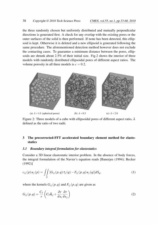
the three randomly chosen but uniformly distributed and mutually perpendiculardirections is generated first. A check for any overlap with the existing pores or theouter surfaces of the solid is then performed. If none has been detected, this ellip-soid is kept. Otherwise it is deleted and a new ellipsoid is generated following thesame procedure. The aforementioned detection method however does not excludethe contacting cases. To guarantee a minimum distance between the pores, ellip-soids are shrunk about 2.5% of their initial size. Fig.2 shows the interior of threemodels with randomly distributed ellipsoidal pores of different aspect ratios. Thevolume porosity in all three models is c = 0.2.

(a) 1.0λ = (spherical pores) (b) 0.5λ = (c) 2.0λ =

Figure 2: Three models of a cube with ellipsoidal pores of different aspect ratio, λ

defined as the ratio of two radii.

3 The precorrected-FFT accelerated boundary element method for elasto-statics

3.1 Boundary integral formulation for elastostatics

Consider a 3D linear elastostatic interior problem. In the absence of body forces,the integral formulation of the Navier’s equation reads [Banerjee (1994); Becker(1992)]

ci j (p)u j (p) =∫ ∫

S

[Gi j (p,q)τ j (q)−Fi j (p,q)u j (q)]dSq, (1)

where the kernels Gi j (p,q) and Fi j (p,q) are given as

Gi j (p,q) =C1

r

(C3δi j +

∂ r∂xi

∂ r∂x j

)(2)


and

Fi j (p,q) =−C2

r2

{∂ r∂nq

(C4δi j +3

∂ r∂xi

∂ r∂x j

)+ C4

(ni

∂ r∂x j

−n j∂ r∂xi

)}. (3)

In the above equations, n = [n1 n2 n3]T represents the outward unit normal vector,

r (p,q) represents the Euclidean distance between points p and q, and δi j is theKronecker delta function. On smooth boundaries, the solid angle ci j (p) = 0.5δi j.It is δi j when p is inside the domain and 0 when p is outside the domain. Thesubscripts i and j in the above equations denote the index of the degrees of freedomand the Einstein summation convention is implied. The constants C1,C2,C3,C4 inEqs. (2) and (3) are C1 = 1

16πG(1−ν) , C2 = 18π(1−ν) , C3 = 3− 4ν , C4 = 1− 2ν

respectively, where G = E2(1+ν) is the shear modulus, E is the Young’s modulus and

ν is the Poisson’s ratio.

Stress σi j inside the structure can be expressed in terms of the boundary quantitiesas

σi j (p) =∫∫S

[Gσ

ki j (p,q)τk (q)−Fσ

ki j (p,q)uk (q)]dSq, (4)

where the kernels Gσ

ki j and Fσ

ki j are given by

Gσ

ki j (p,q) =C2

r2

{C4

(δki

∂ r∂x j

+δk j∂ r∂xi

−δi j∂ r∂xk

)+ 3

∂ r∂xi

∂ r∂x j

∂ r∂xk

}(5)

Fσ

ki j (p,q) =−2µC2

r3

{ni

[3ν

∂ r∂x j

∂ r∂xk

+C4δ jk

]+n j

[3ν

∂ r∂xi

∂ r∂xk

+C4δik

]+

nk

[3C4

∂ r∂xi

∂ r∂x j

+(1−4ν)δi j

]+3

∂ r∂nq

(C4δi j

∂ r∂xk

+ν

(δ jk

∂ r∂xi

+δik∂ r∂x j

)−5

∂ r∂xi

∂ r∂x j

∂ r∂xk

)}.

(6)

3.2 The precorrected-FFT algorithm for elastostatics

In the conventional BEM, the final influence matrices are dense. This featurehas greatly limited the application scope of the BEM in the modeling of large-scale problems. Fortunately, several acceleration algorithms have been inventedin the past several decades. The combination of the fast algorithms and iterativesolvers has greatly reduced both the memory usage and the computational timerequired. One of the popular acceleration schemes is the precorrected-FFT tech-nique [Phillips and White (1997)]. This scheme is easy to implement and has the


advantage of being relatively kernel independent. Similar to the other accelerationschemes such as the fast multipole method, the main idea of the precorrected-FFTacceleration scheme is that instead of computing the influence matrix entries corre-sponding to the far-field interaction explicitly and then multiplying them with thesources, the far-field interactions are computed directly via an approximate method.More specifically, in the precorrected-FFT (pFFT) technique, a parallelepiped isconstructed to enclose a three-dimensional problem after it has been discretizedinto n surface panels. This parallelepiped is then subdivided into an array of smallcubes so that each small cube contains only a few panels. Fig. 3(a) shows a 2-Dview of a quarter of a discretized 3-D solid block with a spherical cavity locatedat its center. The parallelepiped which has been divided into an 7×7×7 array ofsmall cubes is shown in Fig. 3(b) together with the discretized block. It shouldbe pointed out that the surface panels and the pFFT cubes can intersect with eachother. There is no need to maintain any consistency between the surface panelsand the cubes. The acceleration of surface integration is achieved by exploitingthe fact that the kernels in the surface integrals such as those in Eqs. (2) and (3)have piecewise-smooth convolution form. Thus with the aid of the uniform gridformed by the cubes in the parallelepiped, these integrals can be computed approx-imately using the Fast Fourier Transform technique. To ensure accuracy, such anapproximation is only employed for far-field interactions, that is, integrals in whichthe evaluation point is far away from the field panel (Figure 3(c)). For nearby in-teractions, direct evaluation is required. The main steps in the precorrected-FFTacceleration technique include

(1) Construction and superposition of the 3-D uniform grid and the discretizedproblem domain (Fig. 3(b));

(2) Determination of the near- and far-field for each panel using the cubes of theparallelepiped; for example, for panel P inside cube S, its near field and farfield are illustrated in Fig. 3 (c);

(3) Projection of the panel source onto the surrounding grid points based on poly-nomial interpolation;

(4) Calculation of the grid to grid integration using the Fast Fourier Transforma-tion;

(5) Interpolation of the grid interaction back to panels;

(6) Subtraction of the near-field interaction;

(7) Computation of the near-field interaction using direct calculation;


(8) Summation of the near-field and far-field contributions.

For a detailed description of this technique, readers are referred to Phillips andWhite (1997) and Masters and Ye (2004).

(a) (b) (c)

Near field

Far field

Figure 3: Side views of a problem domain: one quarter of a solid block with aspherical cavity located at its center: (a) surface mesh of the problem domain (852panels); (b) the superimposed 3-D parallelepiped decomposed into 7×7×7 cubesand the surface mesh; (c) illustration of the near field and far field of panel P locatedinside cube S.

3.3 Numerical implementation

A piecewise constant collocation scheme is employed to discretize the integralequation shown in Eq. (1). The surfaces of the solid and each pore are discretizedinto small triangular panels. At each panel, the displacement and the traction areassumed to be constant. The resultant linear system is then solved using the gener-alized minimal residual algorithm (GMRES) [Saad and Schultz (1986)] acceleratedwith the precorrected-FFT technique.

A major challenge in the solution procedure is the accurate evaluation of the nearlysingular and singular integrals which occur quite frequently in porous solids par-ticularly when the porosity is large. In the literature, a variety of methods havebeen proposed and developed for the evaluation of nearly singular integrals [Scud-eri (2008); Ye (2008)], weakly singular integrals [Han and Atluri (2007); Nagarajanand Mukherjee (1993)], strongly singular [Cruse (1969); Ding and Ye (2004); Liu(2000)] and hypersingular integrals [Chen and Hong (1999); Dominguez, Arizaand Gallego (2000); Gao, Yang and Wang (2008); Li, Wu and Yu (2009); Qian,Han and Atluri (2004); Qian, Han, Ufimtsev and Atluri (2004); Sanz, Solis andDominguez (2007); Yan, Cui and Hung (2005)]. In this work, the nonlinear trans-formation technique described by Ye (2008) is employed to compute the nearly


singular integrals. The weakly singular integrals associated with the G kernel (Eq.(2)) are evaluated using the method proposed by Nargarjan and Mukherjee (1993)in which a transformation to the polar coordinate system is employed to eliminatethe near singularity. For the evaluation of strongly singular integrals; that is, thoseassociated with the F kernel, the analytical method proposed by Cruse (1969) isemployed. In this method, each triangular panel is first divided into three subtri-angles with the centroid of the origin panel being the common vertex as illustratedin Fig. 4. A local coordinate system with the origin at the centroid is then set upfor each subtriangle. For example, for the subtriangle c20, a local coordinate sys-tem ξ1ξ2 is constructed so that the axis ξ1 is parallel to the edge and the axis ξ2 isperpendicular to the edge. The integration of the kernel C2C4

1r2

(ni

∂ r∂x j−n j

∂ r∂xi

)on

this subtriangle can then be obtained analytically as

Ic20i j =−C2C4εi jke1k [log(ξ1 + r)]20 , (7)

where εi jk is the permutation tensor, e1k is the projection of the unit vector of alongξ1-axis on the k-th global axis, and the variable r represents the distance between apoint on the edge and the centroid of the original panel c.

0

c1

2

2ξ1ξ

Figure 4: Illustration of the local coordinate system of the subtriangle c20.

It should be noted that due to flat panels, the integral corresponding to the first termin the F kernel (Eqn. (3)) vanishes because ∂ r/∂nq ≡ 0.

4 Theoretical models

Several theoretical schemes are employed to calculate the effective elastic prop-erties of porous materials with spherical pores. These properties are used in theperformance comparison presented in Section 5. Throughout the rest of the paper,the effective shear, bulk, Young’s moduli and Poisson’s ratio are denoted as G,K,Eand v, respectively. Letters with subscript m represent material properties of thematrix.


4.1 Self-consistent method

By setting both the shear and bulk moduli of inclusions to be zero in Eqs. (2-6)-(2-10) in Budiansky (1965), the effective shear and bulk moduli of porous materialswith spherical pores satisfy the following two equations:

1G

=1

Gm+

c(1−β )G

(8)

1K

=1

Km+

c(1−α)K

, (9)

where α = 1+ν

3(1−ν) = 3K3K+4G ,β = 2(4−5ν)

15(1−ν) = 6(K+2G)5(3K+4G) . Further mathematic manipula-

tion yields the following equations from which the effective shear and bulk modulican be readily obtained.

8G2 +[3(3− c)Km−8Gm +20 · c ·Gm]G+(18c−9)KmGm = 0, (10)

K =4(1− c)KmG4G+3cKm

(11)

4.2 Differential scheme

Based on the idea of realization, the expressions [Norris (1985)] for the effectivebulk and shear moduli of porous materials in the differential form are obtained as,

dKdc

=−K3K +4G

4G1

1− c(12)

dGdc

=−G15K +20G9K +8G

11− c

(13)

with the initial conditions of K(0) = Km and G(0) = Gm. Using the central differ-ence method one can obtain the numerical values of K and G from Eqs. (12) and(13).

4.3 Generalized self-consistent method

In this method, the inclusions/pores are coated with a matrix shell and then areembedded in an infinite effective material with as-yet-unknown elastic constants[Benveniste (2008); Christensen and Lo (1979)]. Formulas for the effective prop-erties of porous materials can be derived and are given as,

KKm

= 4(1− c)Gm

4Gm +3cKm(14)


A(G

Gm)2 +2B

GGm

+C = 0 (15)

where

A = 4(7−10vm)(7−5vm)+50(7−12vm +8v2m)c−252c5/3 +25(7− v2

m)c7/3

+ 2(4− 5vm)(7 + 5vm)c10/3,

B =−(3/2)(7−5vm)(7−15vm)−75vm(3− vm)c+252c5/3−25(7− v2m)c7/3

+(1/2)(7 + 5vm)(5vm−1)c10/3,

C =−(7−5vm)(7+5vm)+25(7− v2m)c−252c5/3 +25(7− v2

m)c7/3

− (7 + 5vm)(7− 5vm)c10/3.

For more detailed information please refer to Eqs.(3.15-3.18) in [Christensen andLo (1979)] or Eqs.(31-33) in [Lu, Huang and Wang (1995)].

4.4 Mori-Tanaka method

The elastic moduli of porous materials can be obtained from Benveniste (1987) as,

KKm

= 4(1− c)Gm

4Gm +3cKm(16)

GGm

= 1− 5(3Km +4Gm)3(3+2c)Km +4(2+3c)Gm

c (17)

4.5 Hashin bounds

Based on the “variational principle”, Hashin et al [Hashin (1962) ; Hashin andShtrikman (1963)] derived the upper and lower bounds for both bulk and shearmoduli of composite materials. When the inclusions/pores are spherical, the boundsof the bulk modulus coincide which yield the exact solution for the bulk modulusas shown in Eqn. (18).

KKm

= 4(1− c)Gm

4Gm +3cKm(18)

This formula is identical to that obtained from the generalized self-consistent methodand Mori-Tanaka method shown in Eqs. (14) and (16). Unfortunately the boundsfor the shear modulus do not coincide. Hashin (1962) provided a simple formulawhich produces an intermediate value between the two bounds.

GGm

= 1− 5(3Km +4Gm)3(3+2c)Km +4(2+3c)Gm

c (19)


5 Validation of the pFFT accelerated BEM

In this section, numerical simulations of two examples using the developed pFFTaccelerated BEM code are presented. Results are compared with the analyticalsolution and the solution obtained from ANSYS, a commercial FEM software.

5.1 A pressurized thick-wall cylindrical vessel

A 3D pressurized thick-wall cylindrical vessel with an inner radius of ri = 3m andan outer radius of ro = 6m is subject to an inner pressure of pi = 1Pa and a zeroouter pressure. The Young’s modulus and the Poisson’s ratio of the vessel materialare Em = 1.0× 105Pa and νm = 0.3, respectively. The radial displacement of thevessel as a function of the radial distance r can be derived analytically as [Becker(1992); Lu and Luo (1997)]

ur (r) = c1r +c2

r(20)

where c1 = 1E∗

(1−ν∗)r2i pi

r2o−r2

i, c2 = 1

E∗(1+ν∗)r2

i r2o pi

r2o−r2

iand E∗ = Em

1−ν2m,ν∗ = νm

1−νm.

Substituting the parameters associated with the vessel into Eqn. (20), one obtainsc1 = 26/15× 10−6 ≈ 1.73333× 10−6 and c2 = 1.56× 10−5m2. Therefore, theanalytical solutions of the radial displacements of the inner and outer cylindricalsurfaces are ur (3) =57.2 µm and ur (6) =36.4 µm, respectively.

The developed 3-D pFFT accelerated BEM code is employed to calculate the ra-dial displacement of the pressurized vessel. Due to symmetry, only a quarter ofthe structure is modeled. Fig. 5 shows the simulation domain together with its twodiscretized models. The height of the simulation model is set to be H = 9m. Inorder to model the infinitely long cylinder, symmetrical boundary conditions areapplied at the top and the bottom surfaces. The simulated radial displacements atthe inner and outer surfaces are listed in Table 1. Several different discretizationsare employed starting from the coarse mesh with 60 triangular panels to the finestmesh with 59392 panels. The mesh is refined in such a way that the number of theelements along the edges of the structure is doubled in each refinement. Resultsobtained from the direct BEM simulations, i.e., without the acceleration, are alsopresented in Table 1 for comparison. Due to the limited memory of our computer,the finest discretization that can be simulated in the direct calculation is 3712. Over-all, the linear convergence rate is observed in both sets of the results. In addition,the accuracies of the two sets of results are also comparable, indicating that theacceleration via the pFFT technique does not affect both the convergence rate andthe accuracy. Also listed in Table 1 are the consumed memory and the CPU timeassociated with each method. To provide a clear picture of both the memory and


the CPU time, Fig. 6 plots the consumed memory and the CPU time as functions ofthe number of panels. The lines corresponding to O(n), O(n logn) and O

(n2)

arealso plotted for reference. It is evident that both the CPU time and memory usageof the pFFT accelerated BEM are of O(n logn), a great improvement from O

(n2)

particularly when n is large.

(a) One quarter of the vessel (b) Discretization with 60 panels (c) Discretization with 3712 panels Figure 5: Simulation model and surface mesh for a pressurized thick-wall cylindri-

cal vessel.

Table 1: Illustration of the convergence and efficiency of the pFFT BEM and thedirect BEM

MethodNumber of panels

60 232 928 3712 14848 59392

pFFT BEM

memory (MB) 3 21 51 174 1445 6509time (s) 2 11 36 156 1408 8719uo

r (µm) 37.6250 36.7542 36.5204 36.5133 36.5062 36.4423error 3.37% 0.97% 0.33% 0.31% 0.29% 0.12%

uir(µm) 62.6100 59.0800 57.9006 57.6281 57.4708 57.3066error 9.46% 3.29% 1.22% 0.75% 0.47% 0.19%

Direct BEM

memory (MB) 3 23 266 4251time (s) 2 14 228 4986uo

r (µm) 37.6250 36.7542 36.5742 36.4971error 3.37% 0.97% 0.48% 0.27%

uir(µm) 62.6100 59.0800 58.0275 57.6000error 9.46% 3.29% 1.45% 0.70%

5.2 A pressurized cube with a spherical cavity at its center

To further validate the in-house code based on the fast pFFT BEM for elastostaticproblems, the case of a cube with a spherical cavity located at its center is simu-lated. Again the material is characterized by Young’s modulus Em = 1.65×105Pa


100 1000 10000 1000000.1

1

10

100

1000

10000

100000

1000000

1E7

mem

ory

or ti

me

number of panels

pFFT BEM memory (MB) pFFT time (s) Direct BEM memory (MB) Direct BEM time (s) O(n2) O(n*log(n)) O(n)

Figure 6: Consumed memory and computational time as functions of the numberof panels

and Poisson’s ratio νm = 0.33. The length of the cube is set to be 1 m and the radiusof the spherical cavity is 0.15 m. Uniform normal pressure P = 1 Pa is applied atthe surfaces of z =±0.5. Because of symmetry, only one octant of the cube is mod-eled as shown in Fig. 7. The boundary conditions of the simulation model are thatthe normal pressure of 1 Pa is set at z = 0.5; zero traction is applied at the surfaceof the cavity and the outer surfaces specified by x =−0.5 and y =−0.5. All othersurfaces are treated as the symmetric surfaces.

The simulated displacements along the z-direction, uz, at point A(0,0,0.5) at dif-ferent discretizations are listed in Table 2. Due to the lack of the analytical solutionin this case, numerical solution,uz =−3.1265µm, obtained from the finite elementanalysis using the commercial software ANSYS with 33132 SOLID95 elementsand 47752 nodes is used as the reference value for the error calculation. Again,the accuracy of the pFFT accelerated BEM and its linear convergence are demon-strated.

6 Mechanical characterization of porous solids

The effective elastic properties of porous materials can be obtained based on theprinciple of energy equivalence; that is, by equating the total strain energy of arepresentative sample of the porous material subject to a specific loading to thetotal strain energy of the same sample subject to the same loading but made of aneffective homogeneous material, of which the material properties are to be found.


(a) Simulation model (b) Surface mesh with 220 panels

(0,0,0.5)A

Figure 7: Model and surface discretization of a cube with a spherical cavity.

Table 2: Illustration of the convergence and efficiency of the fast pFFT BEM andits comparison with the direct BEM

MethodNumber of panels

220 852 3350 13366

pFFT BEM

memory (MB) 8 41 168 599time (s) 6 14 157 503

uz (A)µm -3.168 -3.151 -3.134 -3.131error 1.33% 0.78% 0.24% 0.14%

Direct BEM

memory (MB) 22 235time (s) 13 182

uz (A)µm -3.160 -3.148error 1.07% 0.69%

The loading can be either a specified displacement or a specified traction boundarycondition, which yields an upper bound or a lower bound for the effective Young’s,bulk and shear moduli respectively. For Poisson’s ratio, an upper bound is obtainedif a traction boundary is prescribed while a lower bound is obtained by applying adisplacement loading.

Both effective Young’s modulus E and Poisson’s ratio can be calculated by apply-ing a uniaxial traction or a uniaxial displacement to the sample. To determine theeffective bulk modulus, a uniform normal traction σ0n or a linear displacementfield corresponding to an isotropic strain ε0 is applied on the outer surfaces of a


representative sample. Based on the “energy equivalence”, the two bounds of the

bulk modulus can be obtained as KL = σ0VM∑j=1

(n·uA) j

and KU =

M∑j=1

(T·xA) j

9ε0V , where KL

and KU denote the lower and the upper bounds, respectively, M is the total numberof elements on the outer surfaces, (n,A,x,u,T) j represent the outward unit normalvector, the area, the centroid, the displacement and the traction of the j-th element,and V is the volume of the representative sample. Similarly, the effective shear

modulus is obtained as GL = τ2VM∑j=1

(T·uA) j

or GU =

M∑j=1

(T·xA) j

4γ2V , corresponding to the

loading conditions of T1 = τn2,T2 = τn1,T3 = 0 and u1 = γx2,u2 = γx1,u3 = 0 ,respectively. In this work, both bounds are obtained and the average value of thetwo bounds serves as the simulated effective property.

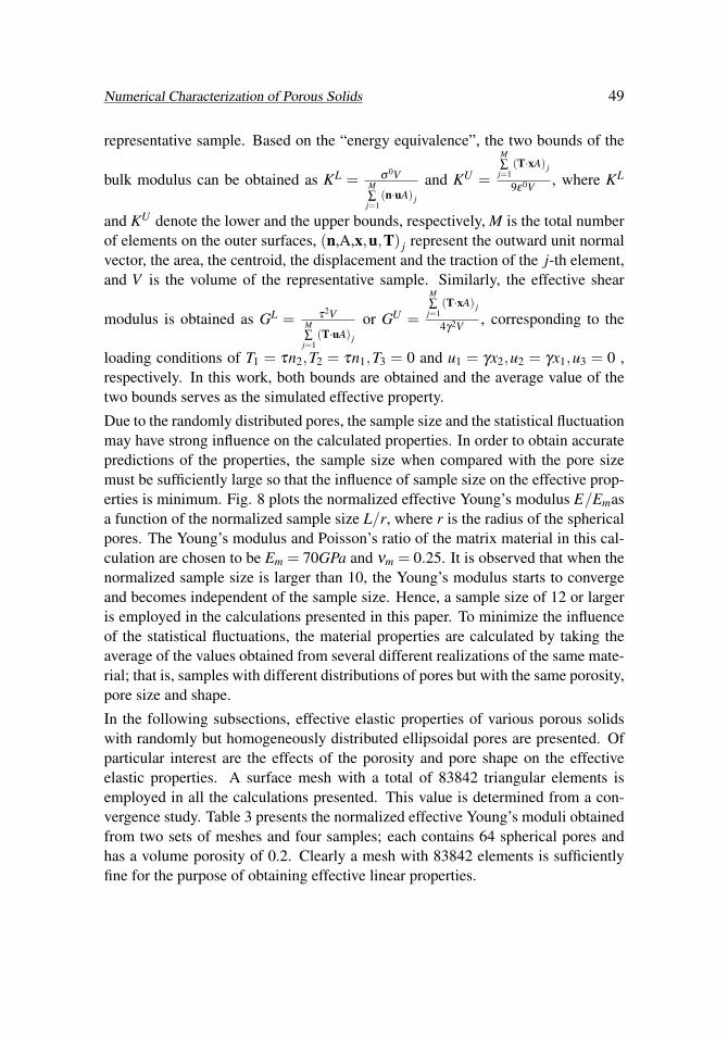
Due to the randomly distributed pores, the sample size and the statistical fluctuationmay have strong influence on the calculated properties. In order to obtain accuratepredictions of the properties, the sample size when compared with the pore sizemust be sufficiently large so that the influence of sample size on the effective prop-erties is minimum. Fig. 8 plots the normalized effective Young’s modulus E/Emasa function of the normalized sample size L/r, where r is the radius of the sphericalpores. The Young’s modulus and Poisson’s ratio of the matrix material in this cal-culation are chosen to be Em = 70GPa and νm = 0.25. It is observed that when thenormalized sample size is larger than 10, the Young’s modulus starts to convergeand becomes independent of the sample size. Hence, a sample size of 12 or largeris employed in the calculations presented in this paper. To minimize the influenceof the statistical fluctuations, the material properties are calculated by taking theaverage of the values obtained from several different realizations of the same mate-rial; that is, samples with different distributions of pores but with the same porosity,pore size and shape.

In the following subsections, effective elastic properties of various porous solidswith randomly but homogeneously distributed ellipsoidal pores are presented. Ofparticular interest are the effects of the porosity and pore shape on the effectiveelastic properties. A surface mesh with a total of 83842 triangular elements isemployed in all the calculations presented. This value is determined from a con-vergence study. Table 3 presents the normalized effective Young’s moduli obtainedfrom two sets of meshes and four samples; each contains 64 spherical pores andhas a volume porosity of 0.2. Clearly a mesh with 83842 elements is sufficientlyfine for the purpose of obtaining effective linear properties.


5 6 7 8 9 10 11 12 13 140.45

0.5

0.55

0.6

0.65

0.7

0.75

L/ r

E/E m

c=0.3c=0.2

Figure 8: Normalized Young’s modulus as a function of the normalized samplesize.

Table 3: Convergence Study

E/Em 83842 elements 191814 elements Relative error (%)Sample 1 0.6441 0.6400 0.6406Sample 2 0.6398 0.6357 0.6449Sample 3 0.6429 0.6387 0.6576Sample 4 0.6437 0.6396 0.6410Average 0.6426 0.6385 0.6421

6.1 Porosity effect

The simulated effective properties of porous samples with different porosities areplotted in Fig.9. The error bars indicate the range of variations caused by dif-ferent realizations and the dots represent the average values obtained from differ-ent realizations. As expected, the effective Young’s modulus, shear modulus andbulk modulus corresponding to the case with a prescribed traction boundary con-dition are lower than that of the case when a displacement boundary condition isprescribed. On the contrary, Poisson’s ratio obtained from cases with a tractionboundary condition is larger than that from cases with a displacement boundarycondition. The differences between the two bounds at different porosities are listedin Table 4. It is observed that the difference increases with the increased porosity.


All three elastic moduli decrease with the increasing porosity and exhibit a slightlynon-linear dependence on the porosity. The dependence of Poisson’s ratio on theporosity is however much weaker and is subject to a larger fluctuation. Despitethe variation, a steady reduction in Poisson’s ratio is observed before the porosityreaches 0.35. It seems that Poisson’s ratio starts to increase with the porosity after0.35.

0 0.1 0.2 0.3 0.4

0.4

0.5

0.6

0.7

0.8

0.9

1

Porosity (c)

E/E m

Displacement BCsStress BCs

0 0.1 0.2 0.3 0.4

0.22

0.225

0.23

0.235

0.24

0.245

0.25

0.255

0.26

Porosity (c)

ν


(a) Normalized Young’s modulus (b) Poisson’s ratio

0 0.1 0.2 0.3 0.4

0.4

0.5

0.6

0.7

0.8

0.9

1

Porosity (c)

K/K

m


0 0.1 0.2 0.3 0.4

0.3

0.4

0.5

0.6

0.7

0.8

0.9

1

Porosity (c)

G/G

m


(c) Normalized bulk modulus (d) Normalized shear modulus Figure 9: Simulated effective elastic properties of a porous solid with spherical

pores as functions of its porosity.


Table 4: Relative differences of elastic properties between the two bounds

Relative difference c=0.1 c=0.2 c=0.25 c=0.3 c=0.35 c=0.4∆E/Em(%) 0.79 2.09 2.54 3.21 3.87 5.14

∆v(%) 0.05 0.10 0.51 0.58 0.79 1.61∆K/Km(%) 0.95 2.17 2.76 3.95 4.41 5.19∆G/Gm(%) 1.84 4.67 5.76 7.98 9.41 10.69

6.2 Shape effect

The effects of pore shape on the Young’s modulus and Poisson’s ratio are studiedby varying the radius along one semi-principal axis of the ellipsoid while keepingthe radii along the other two semi-principal axes fixed, i.e., by varying the aspectratio of the ellipsoidal pores, λ , defined as the ratio of a and b, where a and b arethe radii of the ellipsoid along two principal axes. The generation of randomly dis-tributed ellipsoidal pores with a specific λ is described in Section 2. The orientationof the ellipsoids is random but uniformly distributed. At each λ , four samples withthe same porosity are constructed and modeled. The simulated Young’s modulus asa function of the aspect ratios is plotted in Fig.10, which demonstrates a decreas-ing Young’s modulus with the decreased λ . Such a trend is consistent with thatobserved in He, Lim and Lim (2008), in which the effective Young’s moduli weresimulated for cubes containing uniformly distributed ellipsoidal voids of differentaspect ratio. It was found that the stiffness of the cube varied with the aspect ratioand the orientation of the voids. When the angle between the major axis of the el-lipsoid and the z-axis is smaller than 45◦, the stiffness increases with the increasedaspect ratio. It decreases with the increased aspect ratio when the angle is largerthan 45◦. However, when compared with the case of spherical pores, the amountof change in the stiffness is not equal in the two cases. The increase in the stiffnesswhen the angle is smaller than 45◦ is larger than the amount of the reduction in thestiffness when the angle is larger than 45◦. Therefore, in our case, even when theangle is uniformly distributed, the effective Young’s modulus of the cube with ran-domly distributed ellipsoidal pores increases with the increased aspect ratio. Dueto the large variations, the effect of pore shape on Poisson’s ratio is inconclusive.

6.3 Comparison between theoretical models and numerical simulations

It is of interest to compare the numerical predictions of effective elastic propertiesof porous solids with those obtained from various theoretical models. Due to thevarious assumptions employed in the theoretical models, numerical characteriza-tion of realistic materials is a viable approach for the evaluation of the performance


0.1 0.15 0.2 0.25 0.30.45

0.5

0.55

0.6

0.65

0.7

0.75

0.8

0.85

Porosity (c)

E/E m

λ=1.0

λ=1.5

λ=3.0

0.1 0.15 0.2 0.25 0.3

0.23

0.232

0.234

0.236

0.238

0.24

0.242

0.244

0.246

0.248

0.25

Porosity (c)

ν

λ=1.0

λ=1.5

λ=3.0

(a) normalized Young’s modulus (b) Poisson’s ratio Figure 10: Simulated Young’s modulus and Poisson ratio of porous solids withdifferent ellipsoidal pores.

of these models. In Fig. 11, Young’s modulus, Poisson’s ratio, bulk and shear mod-uli of porous solids with 125 randomly but homogeneously distributed sphericalpores obtained from numerical simulations and various theoretical models are pre-sented. Again, the numerical values are the averages of the upper and lower bounds.Among the four theoretical schemes, the performances of Mori-Tanaka’s methodand the generalized self-consistent method (GSCM) are comparable in the predic-tion of the effective Young’s, bulk and shear moduli with the GSCM’s performancebeing slightly better. Both models give much better predictions than the other twomethods. The self-consistent method yields the worst predictions of all properties.All methods except Mori-Tanaka’s method do not produce good predictions of theeffective Poisson’s ratio. The good performance of Mori-Tanaka’s scheme in thepresent examples is not surprising as this scheme is derived for materials with ran-domly distributed ellipsoidal inclusions. As illustrated in Benveniste (1987), theinclusion/pore interaction is accounted in a similar way as that in the GSCM whichexplains to a certain extent the similar performance of the two methods.

7 Summary

A 3D precorrected-FFT accelerated BEM approach is developed for the linear elas-tic analysis of porous solids with randomly distributed pores of arbitrary shape andsize. This approach enables the direct simulation of porous solids with large poros-ity; hence accurate predictions of elastic behavior of realistic porous solids can beproduced. The developed BEM code is validated using two examples in which


0 0.1 0.2 0.3 0.4

0.2

0.3

0.4

0.5

0.6

0.7

0.8

0.9

1

Porosity (c)

E/E m

Simulation

SCM

DS

GSCM

Mori−Tanaka

0 0.1 0.2 0.3 0.4

0.2

0.21

0.22

0.23

0.24

0.25

Porosity(c)

ν

SimulationSCMDSGSCMMori−Tanaka

(a) Normalized Young’s modulus (b) Poisson’s modulus

0 0.1 0.2 0.3 0.4

0.2

0.3

0.4

0.5

0.6

0.7

0.8

0.9

1

Porosity(c)

K/K m


0 0.1 0.2 0.3 0.4

0.2

0.3

0.4

0.5

0.6

0.7

0.8

0.9

1

Porosity(c)

G/G

m


(c) Normalized bulk modulus (d) Normalized shear modulus

Figure 11: Comparison between theoretical schemes and numerical simulations

the analytical solution and the numerical solution obtained by finite element cal-culations are used for comparison. The accuracy and the efficiency of the BEMapproach have been demonstrated in both examples. As an application of the de-veloped fast BEM approach, the Young’s, shear and bulk moduli and Poisson’s ratioof porous solids with spherical pores of different porosities are calculated. Both up-per and lower bounds are obtained and the average values of the two bounds areused as the numerical predictions of the elastic properties. The largest porosity sim-ulated in the present work is 0.4. This value is largely limited by the methods formodel generation. The effects of porosity and pore shape on elastic properties are


investigated using numerical simulations. Despite being macroscopically isotropic,the Young’s modulus of materials with ellipsoidal pores depends on the aspect ratioof the ellipsoids.

The developed approach is also employed to evaluate the performances of vari-ous theoretical schemes for the predictions of effective material properties of com-posite/porous materials. Overall, both the generalized self-consistent method andMori-Tanaka’s method perform quite well compared to the self-consistent methodand the differential scheme by Norris. The generalized self-consistent method givesthe best approximations to the three elastic moduli, while Mori-Tanaka methodagrees well with the numerical value of Poisson’s ratio.

Acknowledgement: This research has been supported by Hong Kong ResearchGrants Council under Competitive Earmarked Research Grant 621607.

References

Aimi, A.; Diligenti, M.; Lunardini, F.; Salvadori, A. (2003): A new applicationof the panel clustering method for 3D SGBEM. CMES: Computer Modeling inEngineering and Sciences, 4(1): 31-50.

Aoki, S.; Amaya, K.; Urago, M.; Nakayama, A. (2004): Fast multipole boundaryelement analysis of corrosion problems. CMES: Computer Modeling in Engineer-ing and Sciences, 6(2): 123-132.

Banerjee, P. K. (1994): Boundary element methods in engineering. McGraw-Hillbook Company.

Bebendorf, M.; Rjasanow, S. (2003): Adaptive low-rank approximation of collo-cation matrices. Computing, 70(1): 1-24.

Becker, A. A. (1992): The boundary element method in engineering. McGraw-HillBook Company.

Benveniste, Y. (1987): A new approach to the application of Mori-Tanaka’s theoryin composite materials. Mechanics of Materials, 6(2): 147-157.

Benveniste, Y. (2008): Revisiting the generalized self-consistent scheme in com-posites: Clarification of some aspects and a new formulation. Journal of the Me-chanics and Physics of Solids, 56(10): 2984-3002.

Brancati, A.; Aliabadi, M. H.; Benedetti, I. (2009):Hierarchical adaptive crossapproximation GMRES Technique for solution of acoustic problems using the bound-ary element method, CMES: Computer Modeling in Engineering & Sciences, 43(2),149-172.

Budiansky, B. (1965): On the elastic moduli of some heterogeneous materials.


Journal of the Mechanics and Physics of Solids, 13(4): 223-227.

Chen, J. T.; Hong, H. K. (1999): Review of dual boundary element methodswith emphasis on hypersingular integrals and divergent series. Applied MechanicsReviews, 52(1): 17-32.

Chew, W. C.; Song ,J. M.; Cui, T. J.; Velamparambil, S.; Hastriter, M. L.; Hu,B. (2004): Review of large scale computing in electromagnetics with fast integralequation solvers. CMES: Computer Modeling in Engineering and Sciences, 5(4):361-372.

Christensen, R. M. (1998): Two theoretical elasticity micromechanics models.Journal of Elasticity, 50(1): 15-25.

Christensen, R. M.; Lo, K. H. (1979): Solutions for effective shear properties inthree phase sphere and cylinder models. Journal of the Mechanics and Physics ofSolids, 27(4): 315-330.

Criado, R.; Ortiz, J. E.; Mantic, V.; Gray, L. J.; París, E. (2007): Boundaryelement analysis of three-dimensional exponentially graded isotropic elastic solids.CMES: Computer Modeling in Engineering and Sciences, 22(2): 151-164.

Cruse, T. A. (1969): Numerical solutions in three dimensional elastostatics. Inter-national Journal of Solids and Structures, 5(12): 1259-1274.

Day, A. R.; Snyder, K. A.; Garboczi, E. J.; Thorpe, M. F. (1992): The elasticmoduli of a sheet containing circular holes. Journal of the Mechanics and Physicsof Solids, 40(5): 1031-1051.

Ding, J.; Ye, W. (2004): A fast integral approach for drag force calculation dueto oscillatory slip Stokes flows. International Journal for Numerical Methods inEngineering, 60(9): 1535-1567.

Dominguez, J.; Ariza, M. P.; Gallego, R. (2000): Flux and traction boundary el-ements without hypersingular or strongly singular integrals. International Journalfor Numerical Methods in Engineering, 48(1): 111-135.

Frangi, A.; Gioia, A. D. (2005): Multipole BEM for the evaluation of dampingforces on MEMS. Computational Mechanics, 37(1): 24-31.

Gao, X. W.; Yang, K.; Wang, J. (2008): An adaptive element subdivision tech-nique for evaluation of various 2D singular boundary integrals. Engineering Anal-ysis with Boundary Elements, 32(8): 692-696.

Gatt, J. M.; Monerie, Y.; Laux, D.; Baron, D. (2005): Elastic behavior of porousceramics: Application to nuclear fuel materials. Journal of Nuclear Materials,336(2-3): 145-155.

Greengard, L.; Rokhlin, V. (1997): A new version of the fast multipole methodfor the Laplace equation in three dimensions. Acta Numer., 6: 229-269.


Gusev, A. A. (1997): Representative volume element size for elastic composites:A numerical study. Journal of the Mechanics and Physics of Solids, 45(9): 1449-1459.

Hackbusch, W.; Nowak, Z. P. (1989): On the fast matrix multiplication in theboundary element method by panel clustering. Numer. Math. 54: 463-491.

Han, Z. D.; Atluri, S. N. (2007): A systematic approach for the development ofweakly-singular BIEs. CMES: Computer Modeling in Engineering and Sciences,21(1): 41-52.

Hashin, Z. (1962): The elastic moduli of heterogeneous materials. Journal ofApplied Mechanics, Transactions ASME.

Hashin, Z.; Shtrikman, S. (1963): A variational approach to the theory of theelastic behavior of multiphase materials. J. Mech. Phys. Solids, 13: 213-222.

He, X. F.; Lim, K. M.; Lim, S. P. (2008): Fast BEM solvers for 3D Poisson-typeequations. CMES: Computer Modeling in Engineering and Sciences, 35(1): 21-48.

He, X. F.; Lim, K. M.; Lim, S. P. (2008): A fast elastostatic solver based onfast Fourier transform on multipoles (FFTM). International Journal for NumericalMethods in Engineering, 76(8): 1231-1249.

Hill, R. (1965): A self-consistent mechanics of composite materials. Journal of theMechanics and Physics of Solids, 13(4): 213-222.

Hu, N.; Wang, B.; Tan, G. W.; Yao, Z. H.; Yuan, W. F. (2000): Effective elasticproperties of 2-D solids with circular holes: Numerical simulations. CompositesScience and Technology, 60(9): 1811-1823.

Hwang, K. C.; Huang, Y., (1999). Constitutive relationship of solids. TsinghuaUniversity Press, Beijing.

Kari, S.; Berger, H.; Rodriguez-Ramos, R.; Gabbert, U. (2007): Computationalevaluation of effective material properties of composites reinforced by randomlydistributed spherical particles. Composite Structures, 77(2): 223-231.

Kari, S.; Berger, H.; Rodriguez-Ramos, R.; Gabbert, U. (2007): Numericalevaluation of effective material properties of transversely randomly distributed uni-directional piezoelectric fiber composites. Journal of Intelligent Material Systemsand Structures, 18(4): 361-372.

Karlis, G. F.; Tsinopoulos, S. V.; Polyzos, D.; Beskos, D. E. (2008): 2D and 3Dboundary element analysis of mode-I cracks in gradient elasticity. CMES: Com-puter Modeling in Engineering and Sciences, 26(3): 189-207.

La Mantia, M.; Dabnichki, P. (2008): Unsteady 3D boundary element method foroscillating wing. CMES: Computer Modeling in Engineering and Sciences, 33(2):131-153.


Li, J.; Wu, J. M.; Yu, D. H. (2009): Generalized extrapolation for computation ofhypersingular integrals in boundary element methods. CMES: Computer Modelingin Engineering and Sciences, 42(2): 151-175.

Liu, Y. (2006): A new fast multipole boundary element method for solving large-scale two-dimensional elastostatic problems. International Journal for NumericalMethods in Engineering, 65(6): 863-881.

Liu, Y.; Nishimura, N.; Otani, Y. (2005): Large-scale modeling of carbon-nanotubecomposites by a fast multipole boundary element method. Computational Materi-als Science, 34(2): 173-187.

Liu, Y. J. (2000): On the simple-solution method and non-singular nature of theBIE/BEM - a review and some new results. Engineering Analysis with BoundaryElements, 24(10): 789-795.

Liu, Y. J.; Nishimura, N.; Otani, Y.; Takahashi, T.; Chen, X. L.; Munakata, H.(2005): A fast boundary element method for the analysis of fiber-reinforced com-posites based on a rigid-inclusion model. Journal of Applied Mechanics, Transac-tions ASME, 72(1): 115-128.

Lu, M. W.; Luo, X. F., (1997). Fundamental elasticity theory. Tsinghua UniversityPress, Beijing.

Lu, Z.; Huang, Z.; Wang, R. (1995): Determination of effective moduli for foamplastics based on three phase spheroidal model. Acta Mechanica Solida Sinica,8(4): 294-302.

Masters, N.; Ye, W. (2004): Fast BEM solution for coupled 3D electrostatic andlinear elastic problems. Engineering Analysis with Boundary Elements, 28(9):1175-1186.

Mori, T.; Tanaka, K. (1973): Average stress in matrix and average elastic energyof materials with misfitting inclusions. Acta Metallurgica, 21(5): 571-574.

Nagarajan, A.; Mukherjee, S. (1993): A mapping method for numerical evalua-tion of two-dimensional integrals with 1/r singularity. Computational Mechanics,12(1-2): 19-26.

Norris, A. N. (1985): A differential scheme for the effective moduli of composites.Mechanics of Materials, 4(1): 1-16.

Ong, E. T.; Lim, K. M.; Lee, K. H.; Lee, H. P. (2003): A fast algorithm forthree-dimensional potential fields calculation: Fast Fourier Transform on Multi-poles. Journal of Computational Physics, 192(1): 244-261.

Owatsiriwong, A.; Phansri, B.; Park, K. H. (2008): A cell-less BEM formulationfor 2D and 3D elastoplastic problems using particular integrals. CMES: ComputerModeling in Engineering and Sciences, 31(1): 37-59.


Phillips, J. R.; White, J. K. (1997): A Precorrected-FFT method for electrostaticanalysis of complicated 3-d structures. IEEE Transactions on Computer-Aided De-sign of Integrated Circuits and Systems, 16(10): 1059-1072.

Qian, Z. Y.; Han, Z. D.; Atluri, S. N. (2004): Directly derived non-hyper-singularboundary integral equations for acoustic problems; their solution through Petrov-Galerkin schemes. CMES: Computer Modeling in Engineering and Sciences, 5(6):541-562.

Qian, Z. Y.; Han, Z. D.; Ufimtsev, P.; Atluri, S. N. (2004): Non-hyper-singularboundary integral equations for acoustic problems, implemented by the collocation-based boundary element method. CMES: Computer Modeling in Engineering andSciences, 6(2): 133-144.

Rintoul, M. D.; Torquato, S. (1997): Reconstruction of the structure of disper-sions. Journal of Colloid and Interface Science, 186(2): 467-476.

Roberts, A. P.; Garboczi, E. J. (2000): Elastic properties of model porous ceram-ics. Journal of the American Ceramic Society, 83(12): 3041-3048.

Saad, Y.; Schultz, M. (1986): GMRES: A generalized minimal residual algorithmfor solving symmetric linear systems. SIAM Journal on Scientific and StatisticalComputing, 7: 856-869.

Sanz, J. A.; Solis, M.; Dominguez, J. (2007): Hypersingular BEM for piezoelec-tric solids: Formulation and applications for fracture mechanics. CMES: ComputerModeling in Engineering and Sciences, 17(3): 215-229.

Scuderi, L. (2008): On the computation of nearly singular integrals in 3D BEMcollocation. International Journal for Numerical Methods in Engineering, 74(11):1733-1770.

Segurado, J.; Gonzalez, C.; Llorca, J. (2003): A numerical investigation of theeffect of particle clustering on the mechanical properties of composites. Acta Ma-terialia, 51(8): 2355-2369.

Segurado, J.; Llorca, J. (2002): A numerical approximation to the elastic prop-erties of sphere-reinforced composites. Journal of the Mechanics and Physics ofSolids, 50(10): 2107-2121.

Simone, A. E.; Gibson, L. J. (1998): Effects of solid distribution on the stiffnessand strength of metallic foams. Acta Materialia, 46(6): 2139-2150.

Soares, J. D.; Vinagre, M. P. (2008): Numerical computation of electromag-netic fields by the time-domain boundary element method and the complex variablemethod. CMES: Computer Modeling in Engineering and Sciences, 25(1): 1-8.

Tan, C. L.; Shiah, Y. C.; Lin, C. W. (2009): Stress analysis of 3D generallyanisotropic elastic solids using the boundary element method. CMES: Computer


Modeling in Engineering and Sciences, 41(3): 195-214.

Wang, H. T.; Hall, G.; Yu, S. Y.; Yao, Z. H. (2008): Numerical simulation ofgraphite properties using X-ray tomography and fast multipole boundary elementmethod. CMES: Computer Modeling in Engineering and Sciences, 37(2):153-174.

Wang, H. T.; Yao, Z. H. (2005): A new fast multipole boundary element methodfor large scale analysis of mechanical properties in 3D particle-reinforced compos-ites. CMES: Computer Modeling in Engineering and Sciences, 7(1): 85-96.

Wang, H. T.; Yao, Z. H. (2008): A rigid-fiber-based boundary element model forstrength simulation of carbon nanotube reinforced composites. CMES: ComputerModeling in Engineering and Sciences, 29(1): 1-13.

Wang, H. T.; Yu, S. Y. (2008): Large-scale numerical simulation of mechani-cal and thermal properties of nuclear graphite using a microstructure-based model.Nuclear Engineering and Design, 238(12): 3203-3207.

Wang, W.; Wang, J.; Kim, M. S. (2001): An algebraic condition for the separationof two ellipsoids. Computer Aided Geometric Design, 18(6): 531-539.

Yan, Z. Y.; Cui, F. S.; Hung, K. C. (2005): Investigation on the normal derivativeequation of helmholtz integral equation in acoustics. CMES: Computer Modelingin Engineering and Sciences, 7(1): 97-106.

Yan, Z. Y.; Hung, K. C.; Zheng, H. (2003): Solving the hypersingular boundaryintegral equation in three-dimensional acoustics using a regularization relationship.Journal of the Acoustical Society of America, 113(5): 2674-2683.

Yang, S. A. (2004): An integral equation approach to three-dimensional acousticradiation and scattering problems. Journal of the Acoustical Society of America,116(3): 1372-1380.

Yao, Z.; Kong, F.; Zheng, X. (2003): Simulation of 2D elastic bodies with ran-domly distributed circular inclusions using the BEM. Electronic Journal of Bound-ary Elements, 1(2): 270-282.

Ye, W. (2008): A new transformation technique for evaluating nearly singular in-tegrals. Computational Mechanics, 42(3): 457-466.

Ye, W.; Wang, X.; Hemmert, W.; Freeman, D.; White, J. (2003): Air damping inlateral oscillating micro resonators: A numerical and experimental study. Journalof Microelectromechanical Systems, 12(5): 1-10.

Zozulya, V. V. (2009): Variational formulation and nonsmooth optimization algo-rithms in elastostatic contact problems for cracked body. CMES: Computer Mod-eling in Engineering and Sciences, 42(3): 187-215.

numerical characterization of porous solids and ... · numerical characterization of porous solids...

Documents