numerical analysis of interior aircraft structures made of de

Treball realitzat per:

Lei Pan

Dirigit per:

Xavier Martínez Garcia

Màster en:

MASTER'S DEGREE IN NUMERICAL METHODS IN ENGINEERING

Barcelona, 05, June 2019

ETSECCPB - Barcelona School of Civil Engineering

TR

EBA

LL F

INA

L D

E MÀSTER

Numerical Analysis of Interior

Aircraft Structures made of

Composite Materials

Contents

I

Contents

Contents ------------------------------------------------------------------------------------------------------------------------ I

Abstract ----------------------------------------------------------------------------------------------------------------------- 1

1 Introduction --------------------------------------------------------------------------------------------------------------- 2

1.1 Background and Motivation -------------------------------------------------------------------------------------- 2

1.2 Objectives ------------------------------------------------------------------------------------------------------------ 2

1.3 Outline --------------------------------------------------------------------------------------------------------------- 3

2 Methodology ------------------------------------------------------------------------------------------------------------- 4

2.1 Finite Element Method -------------------------------------------------------------------------------------------- 4

2.2 Multiscale Homogenization --------------------------------------------------------------------------------------- 6

2.2.1 General Background ------------------------------------------------------------------------------------------ 6

2.2.2 First-order Homogenization ---------------------------------------------------------------------------------- 7

2.2.3 FE2 homogenization ----------------------------------------------------------------------------------------- 10

3 Analysis of the beam --------------------------------------------------------------------------------------------------- 12

3.1 Geometry and boundary conditions ----------------------------------------------------------------------------- 12

3.1.1 Beam model and mesh --------------------------------------------------------------------------------------- 12

3.2 Analysis considering an isotropic material -------------------------------------------------------------------- 13

3.2.1 Material and basic settings ---------------------------------------------------------------------------------- 13

3.2.2 Midspan centralized load case ------------------------------------------------------------------------------ 13

3.2.3 Uniform load case -------------------------------------------------------------------------------------------- 15

3.3 Analysis with a multiscale procedure --------------------------------------------------------------------------- 16

3.3.1 Material, basic settings and RVE --------------------------------------------------------------------------- 16

3.3.2 Midspan centralized load case ------------------------------------------------------------------------------ 17

3.3.3 Uniform load case -------------------------------------------------------------------------------------------- 18

4 Analysis of the airplane interior cabin bin (Hatrack) -------------------------------------------------------------- 21

4.1 Geometry, boundary conditions and sandwich structure ---------------------------------------------------- 21

4.1.1 Model, boundary conditions -------------------------------------------------------------------------------- 21

4.1.2 Mesh, basic settings ------------------------------------------------------------------------------------------ 22

4.1.3 Sandwich structure ------------------------------------------------------------------------------------------- 22

Contents

II

4.2 Analysis considering isotropic materials ----------------------------------------------------------------------- 23

4.2.1 Materials ------------------------------------------------------------------------------------------------------- 23

4.2.2 Results of load case 1 ---------------------------------------------------------------------------------------- 24

4.2.3 Results of load case 2 ---------------------------------------------------------------------------------------- 37

4.2.4 Conclusions---------------------------------------------------------------------------------------------------- 48

4.3 Analysis with a multiscale procedure --------------------------------------------------------------------------- 50

4.3.1 Material, RVEs ----------------------------------------------------------------------------------------------- 50

4.3.2 Results ---------------------------------------------------------------------------------------------------------- 52

4.3.3 Conclusions---------------------------------------------------------------------------------------------------- 72

5 Conclusions -------------------------------------------------------------------------------------------------------------- 73

6 References --------------------------------------------------------------------------------------------------------------- 74

Abstract

1

Abstract

This work is focusing on using the numerical methods based on finite element method and multiscale analysis

to study the aircraft structures made of eco-composite materials. In order to achieve this purpose, the PLCd

code and the GiD pre/postprocess software have been introduced into this work. Before the simulations, the

theories of FEM, multiscale analysis and 𝐹𝐸2 homogenization procedure have been discussed. The

validations of PLCd code is conducted through testing the midspan tension stresses of the simple supported

beam considering isotropic material under two load cases. The solutions given by PLCd code show that the

errors are convergent with the increasing number of elements, no matter which method, with or without

multiscale analysis procedure, is used. Another finding is that using quadratic elements will be more accurate

compared to linear elements. And the stress concentration phenomenon has occurred in the results. The

simulations of the cabin bin with isotropic materials under two load cases are conducted to study the stress

field and the displacement field. The first load case corresponds to having the cabin bin completely loaded,

while the second one corresponds to have only half of the cabin bin loaded. The results give the conclusion

that the load case 1 is more dangerous. For the sandwich structure, the cores have undertaken much smaller

stresses. And the results of the stress field of the cabin bin are meaningful for us since we can take

measurements to avoid the damages on the areas where the stresses are large. The areas having large stresses

include the upside boundary condition areas on the sides, the bottom boundary condition areas on the bottom

plate and the back part, and the cross areas between the bottom plate and sides. Then the eco-composites have

been used in the cabin bin. The results of the simulation show that the application of the honeycomb structure

to the core parts will increase the stresses on it because of its large empty spaces. Consequently, we need to

use highly stiff and highly strong material in the core parts to avoid damages. For the skins, the application of

the eco-composites will help the structure to decrease the stresses on them. And the stresses on the cabin bin

with isotropic materials or eco-composites are both lower than the stress thresholds of corresponding materials.

Key Words: finite element method, composite structure, multiscale analysis, sandwich structure

Introduction

2

1 Introduction

1.1 Background and Motivation

Nowadays, the composite materials have already been widely implemented in aircrafts to build lightweight

structures. Since the composite materials possess excellent mechanical properties like high stiffness while

they are much lighter compared to traditionally used materials. For instance, steels or aluminums. The

important role of composite materials in aircraft industry leads to the reduction of fuel consumption and

increased capability of carrying more clients. However, these composites made of carbon-fibers reinforced

plastics (CFRP) or glass-fibers reinforced plastics (GFRP) all need huge energy consumption in their

producing procedures, which has limited their opportunities to be more economical. Furthermore, the high

cost spent on the recycling of these composite materials is another negative factor. Consequently, with the

endless demanding for more efficient and economical aircrafts, people need to seek other possibilities to solve

these problems exiting in the producing and using phases.

Consequently, the ecologically improved renewable composite materials are under investigations in order to

avoid the problems mentioned above about CFRP and GFRP. Following works are parts of the ECO-

COMPASS project whose target is to develop ecological composite materials that can also be renewed [1].

Because of the lacks of enough researches on the ecological composite materials and the caring about safety,

ECO-COMPASS project focuses on implementing ecological composite materials on the interior and

secondary structures on the aircrafts.

To achieve the aim of designing structures with minimal cost on certification tests, numerical techniques

should be involved in our analysis stage. In this work, finite element method (FEM) is used with the code

PLCd [2], developed for solving composite material problems, on GiD pre/postprocess platform.

1.2 Objectives

The main objective of this work is to simulate the cabin bin, made of sandwich structure, by using the

multiscale analysis method. The following objectives are achieved through the conduction of this work:

i) Presenting the multiscale homogenization formulations and the 𝐹𝐸2 homogenization procedure, which

are the theories of the multiscale analysis of PLCd code.

ii) Conducting the validations of the PLCd code by simulating a simple supported beam to prove its accuracy.

iii) Simulating the cabin bin with isotropic materials to study its displacement field and stress field under

different load cases. Comparing the results of different load cases to find which load case is more dangerous.

iv) Simulating the cabin bin with the eco-composites by using the multiscale analysis procedure to study its

displacement field and stress field. Through the comparison with the results of using isotropic material, the

differences of using the eco-composites will be found.

Introduction

3

1.3 Outline

The following contents are divided to 3 chapters to give a comprehensive view of this work.

In chapter 2, the methodologies related to this work have been introduced. The section 2.1 has taken the

Laplace equation as an example to present the basic theory and procedure of finite element method. The

section 2.2 that introduces the theory of multiscale analysis has 3 parts. The part 2.2.1 describes the general

background of the multiscale analysis. Then the first-order homogenization theory and its formulations are

shown in part 2.2.2. The last part of section 2.2 has presented the 𝐹𝐸2 homogenization algorithm.

In chapter 3, the simulations of the beam are shown, which is aimed at learning the capabilities and the

formulations that have been included in this work. The section 3.1 gives the geometry and boundary conditions

of the beam. And the following section 3.2 has conducted the first analysis of the beam with isotropic material

to learn the program features, mesh requirements and the expected precision on the results. The last section

3.3 is the second analysis of beam conducted by using the multiscale analysis procedure. And the

representative volume element used in this case is corresponding to the isotropic material in section 3.2. Under

this situation, the comparison of the results obtained in section 3.2 and section 3.3 is analyzed.

The chapter 4, which has shown the simulations of the cabin bin, is following the same structure of chapter 3.

The geometry and boundary conditions of the cabin bin are presented in section 4.1. In section 4.2, in order to

learn about the performance of the structure of the cabin bin, the first analysis of the cabin bin is conducted

by considering isotropic materials. In this case, the panel with sandwich structure of the cabin bin has glass

fiber skins (Considered as isotropic material) and a foam core. The last section 4.3 has replaced the isotropic

materials used in section 4.2 with eco-composites and the multiscale analysis procedure is used to study the

complex internal micro-structure of these materials. The results are shown in section 4.3.

Chapter 5 gives some conclusions from the results obtained in above contents.

Methodology

4

2 Methodology

The constitutive laws which are suitable for simple materials are no longer useful when it comes to solving

more complicated composite materials. This new demand, building appropriate constitutive formulations for

composite materials, has promoted several developments to appear in past decades.

Truesdell and Toupin [3] proposed classical mixing theory. Then, other researchers extended this theory by

editing its compatibility assumption to make it be capable of solving any reinforced composite. The Serial-

Parallel theory developed by S. Oller and E. Onate [4, 5] has taken into account the contribution from serial

direction while the classical theory only considers the parallel direction’s effect. Besides the mixing theories,

multiscale homogenization method [6] is another option to help us analyze composite materials. The typical

feature of multiscale homogenization is the concept of representative volume element (RVE) [7], which is the

bridge between macroscale and microscale. RVE should be small enough compared to global domain but also

needs to fulfill the request that it can represent the material’s properties.

Finite element method is the numerical technique chosen for our work to solve the composite materials

structural model based on above serial-parallel and multiscale homogenization theories.

2.1 Finite Element Method

The finite element method (FEM) is a numerical technique for solving partial differential equations [8]

established in numerous scientific areas like solid and fluid mechanics, electromagnetics, thermal problems,

etc. Through several decades’ developments, FEM analysis has shown its unique and powerful charm by

enabling us to get accurate approximated solutions without conducting expensive experiments in our research

and engineering projects. In this work, the FEM is used to simulate the composite materials structure to help

us analyze its stresses and displacements under particular load cases. Following contents briefly introduce the

theory of FEM, taking Laplace equation as an example.

Considering the Laplace equation on one dimension:

−∆𝑢 = 𝑓 𝑜𝑛 𝛺 (2.1)

With boundary conditions:

𝑢 = 𝑢𝐷 𝑜𝑛 𝜕𝛺𝐷 (2.2)

𝜕𝑛𝑢 = 𝑞 𝑜𝑛 𝜕𝛺𝑁 (2.3)

Above is the strong form of Laplace equation. Let’s consider the simplified situation:

𝑢𝐷 = 0 𝑎𝑛𝑑 𝛺 = 𝛺𝐷 (2.4)

We multiply Laplace equation with a test function 𝑣 and integrate on 𝛺:

Methodology

5

− ∫ 𝑣𝛺

∆𝑢𝑑𝑥 = ∫ 𝑣𝑓𝑑𝑥𝛺

𝑜𝑛 𝛺 (2.5)

Integrating by parts with the assumption that 𝑣 = 0 on 𝜕𝛺𝐷:

∫ ∇𝑣𝛺

∙ ∇𝑢𝑑𝑥 = ∫ 𝑣𝑓𝑑𝑥𝛺

𝑜𝑛 𝛺 (2.6)

We can define the following spaces:

𝐿2(𝛺) = {𝑢(𝑥): ∫ 𝑢2𝑑𝑥 < ∞𝛺

} (2.7)

𝐻1(𝛺) = {𝑢 ∈ 𝐿2(𝛺): |∇𝑢| ∈ 𝐿2(𝛺)} 𝑎𝑛𝑑 𝐻01(𝛺) = {𝑢 ∈ 𝐻1(𝛺): 𝑢𝜕𝛺𝐷

= 0} (2.8)

Then, the weak form of Laplace equation which is more general:

𝐹𝑖𝑛𝑑 𝑢 ∈ 𝐻01(𝛺): ∫ ∇𝑣

𝛺


, ∀𝑣 ∈ 𝐻01(𝛺) (2.9)

In order to solve the weak form, we need to replace space 𝐻01(𝛺) with finite-dimensional subset:

𝑉 ≡ 𝐻01(𝛺) (2.10)

Through the change of space, we get the discrete form of the Laplace equation:

𝐹𝑖𝑛𝑑 𝑢 ∈ 𝑉: ∫ ∇𝑣𝛺


, ∀𝑣 ∈ 𝑉 (2.11)

By using finite element mesh we can construct the space 𝑉:

𝑉 = {𝑁1, 𝑁2, … , 𝑁𝑖, … , 𝑁𝑛} (2.12)

Where the 𝑁𝑖 is the shape function having following properties if we use linear shape functions:

𝑁𝑖(𝑥𝑖) = 1 𝑎𝑛𝑑 𝑁𝑖(𝑥𝑗) = 0, 𝑖 ≠ 𝑗 (2.13)

The test function can be written as:

𝑣(𝑥) = 𝑣1𝑁1(𝑥) + 𝑣2𝑁2(𝑥) + ⋯ + 𝑣𝑛𝑁𝑛(𝑥) (2.14)

Consequently, we can get:

𝐹𝑖𝑛𝑑 𝒖 ∈ ℝ𝑛: 𝑢𝑖 ∫ ∇𝑁𝑗(𝑥)𝛺

∙ ∇𝑁𝑖(𝑥)𝑑𝑥 = ∫ 𝑣𝑖𝑓𝑑𝑥𝛺

, 𝑖, 𝑗 ∈ 1,2,3 … , 𝑛 (2.15)

We transform it to linear system:

𝑨𝒖 = 𝒇 (2.16)

Where:

Methodology

6

𝐴𝑖𝑗 = ∫ ∇𝑁𝑗(𝑥)𝛺

∙ ∇𝑁𝑖(𝑥)𝑑𝑥 (2.17)

𝑓𝑖 = ∫ 𝑣𝑖𝑓𝑑𝑥𝛺

(2.18)

Through solving above linear system, we can get 𝒖 solution on the domain.

2.2 Multiscale Homogenization [9]

The multiscale homogenization combined with the concept of representative volume element (RVE) has

achieved a high reputation for its convenience and accuracy on computing the behavior of composite material.

RVE is regarded as a microscopic subregion representing the entire microscale structure from the average

point of view. With the help of RVE, we are able to firstly solve the problems, like strain and stress, on

microscale in the RVE model and then applying the results of RVE model to get the solutions on macroscale.

The constitutive law on macroscale is not needed in multiscale homogenization analysis with RVE concept.

The problem on microscale is boundary value problem (BVP) with particular boundary conditions.

Among the developed multiscale homogenization methods, the first-order homogenization method is one of

the most popular choices. Following is the basic theory of first-order homogenization method.

2.2.1 General Background

In this work, we consider infinitesimal strains. We have two configurations, one is 𝛺0 and another one is

𝛺𝑡.They are respectively the material (reference) configuration and spatial (current) configuration. And the

connection between two configurations is the deformation map 𝝋:

𝝋: 𝛺0 → 𝛺𝑡|𝒙 = 𝝋(𝑿, 𝑡) 𝒙 ∈ 𝛺0 𝑎𝑛𝑑 𝑿 ∈ 𝛺𝑡 (2.25)

And the tangent deformation map 𝑭:

𝑭: 𝛺0 → 𝛺𝑡|𝑑𝒙 = 𝑭(𝑿, 𝑡) ∙ 𝑑𝑿 (2.26)

𝑭 = 𝑔𝑟𝑎𝑑𝝋(𝑿, 𝑡) =𝜕𝝋

𝜕𝑿= ∇𝐱 (2.27)

However, above formulation is not satisfied anymore when we consider the finite material line in a finite

volume. As a result, we need to use Taylor series expression for ∆𝒙 in current configuration:

△ 𝒙 = 𝑭(𝑿0) ∙△ 𝑿 +1

2𝑮(𝑿0):△ 𝑿 ⊗△ 𝑿 + 𝒪(△ 𝑿0

3) (2.28)

Where 𝑮 is the gradient of the deformation gradient tensor and 𝑮 is symmetric:

𝑮 = 𝑔𝑟𝑎𝑑𝑭 = ∇𝑭 (2.29)

Methodology

7

2.2.2 First-order Homogenization

The domain 𝛺 considered in this work is periodic, so the RVE model can represent its microstructure. Figure

2.1 shows the infinitesimal point 𝑿0 and its corresponding RVE around 𝑿0 that we have defined in the material

configuration of the domain.

Figure 2.1. Macrostructure and microstructure around of the point 𝑋0

Since the RVE is considered much smaller than the macroscale as discussed before, For the material point 𝑿𝑢0

in the RVE we can apply the Taylor series to approximate its deformed position 𝒙𝑢0 in spatial configuration:

𝒙𝜇(𝑿0, 𝑿𝜇) ≅ 𝒙𝜇0 + 𝑭(𝑿0) ∙ △ 𝑿𝜇 + 𝒘(𝑿𝜇) (2.30)

△ 𝑿𝜇 = 𝑿𝜇 − 𝑿𝜇0 , 𝑿𝜇 ∈ 𝛺𝜇 (2.31)

𝑿𝜇0 and 𝒙𝜇

0 are respectively the material and spatial coordinate system of the RVE, which equal to zero for

simplification. 𝑿𝜇 represents the original material point of 𝒙𝜇 in material configuration.

By setting:

𝑿𝜇0 = 0, 𝒙𝜇

0 = 0 (2.32)

We get:

𝒙𝜇(𝑿0, 𝑿𝜇) ≅ 𝑭(𝑿0) ∙ 𝑿𝜇 + 𝒘(𝑿𝜇) (2.33)

The displacement field 𝒖𝜇 in RVE:

𝒖𝜇 = 𝒙𝜇 − 𝑿𝜇 (2.34)

Introducing the expression of 𝒙𝜇:

𝒖𝜇 = [𝑭(𝑿0) − 𝑰] ∙ 𝑿𝜇 + 𝒘(𝑿𝜇) (2.35)

Where 𝑰 is the second order unit tensor.

From above displacement field, we can find that 𝒖𝜇 is coupled by the macroscale (𝑭(𝑿0)) and microscale

(𝑿𝜇). Through the average theories introduced by Hill [8], we can build following relationship between the

gradient of deformation tensor on microscale 𝑭𝜇 and the gradient of deformation tensor on macroscale 𝑭:

Methodology

8

𝑭(𝑿0) =1

𝑉𝜇∫ 𝑭𝜇(𝑿0, 𝑿𝜇)𝑑𝑉

𝛺𝜇

(2.36)

𝑉𝜇 is the volume of the RVE in the material configuration.

We have:

𝑭𝜇(𝑿0, 𝑿𝜇) = ∇𝒙𝜇(𝑿0, 𝑿𝜇) ≅ 𝑭(𝑿0) + ∇𝒘(𝑿𝜇) (2.37)

=>

1

𝑉𝜇∫ 𝑭𝜇(𝑿0, 𝑿𝜇)𝑑𝑉

𝛺𝜇

=1

𝑉𝜇∫ ∇𝒙𝜇(𝑿0, 𝑿𝜇)𝑑𝑉

𝛺𝜇

= 𝑭(𝑿0) +1

𝑉𝜇∫ ∇𝒘(𝑿𝜇)𝑑𝑉

𝛺𝜇

(2.38)

=>

𝑭(𝑿0) =1

𝑉𝜇∫ ∇𝒙𝜇(𝑿0, 𝑿𝜇)𝑑𝑉

𝛺𝜇

−1


𝛺𝜇

(2.39)

By applying the divergence theorem, above formulation can be transformed to integration on the surface:

𝑭(𝑿0) =1

𝑉𝜇∫ 𝒙𝜇(𝑿0, 𝑿𝜇) ⊗ 𝑵𝑑𝐴

𝜕𝛺𝜇

−1

𝑉𝜇∫ 𝒘(𝑿𝜇) ⊗ 𝑵𝑑𝐴

𝜕𝛺𝜇

(2.40)

Where 𝜕𝛺𝜇 is the boundaries of RVE in the material configuration and 𝑵 is the outward unit normal on 𝜕𝛺𝜇.

As we can see, the average theory is satisfied only when following equations are true:

1


𝛺𝜇

= 0 𝑎𝑛𝑑 1

𝑉𝜇∫ 𝒘(𝑿𝜇) ⊗ 𝑵𝑑𝐴

𝜕𝛺𝜇

= 0 (2.41)

Which gives the integration restriction on the RVE boundaries.

Next step is to get the microscopic and macroscopic strain tensor. Taking the infinitesimal deformation

framework into account, the strain tensor in the microscale is:

𝑬𝜇(𝑿0, 𝑿𝜇) =1

2(𝑭𝜇(𝑿0, 𝑿𝜇) + 𝑭𝜇

𝑇(𝑿0, 𝑿𝜇)) − 𝑰 (2.42)

=>

𝑬𝜇(𝑿0, 𝑿𝜇) =1

2(𝑭(𝑿0) + 𝑭𝑇(𝑿0)) − 𝑰 +

1

2(∇𝒘(𝑿𝜇) + ∇𝒘(𝑿𝜇)

𝑇) (2.43)

Applying the volume average theory to the microscopic strain tensor:

𝑬(𝑿0) =1

𝑉𝜇∫ 𝑬𝜇(𝑿0, 𝑿𝜇)𝑑𝑉

𝛺𝜇

=1

2(𝑭(𝑿0) + 𝑭𝑇(𝑿0)) − 𝑰 (2.44)

=>

Methodology

9

𝑬𝜇(𝑿0, 𝑿𝜇) = 𝑬(𝑿0) +1

2(∇𝒘(𝑿𝜇) + ∇𝒘(𝑿𝜇)

𝑇) = 𝑬(𝑿0) + 𝑬𝜇

𝝎(𝑿𝜇) (2.45)

𝑬𝜇𝝎(𝑿𝜇) =

1

2(∇𝒘(𝑿𝜇) + ∇𝒘(𝑿𝜇)

𝑇) (2.46)

The Hill-Mandel energy condition [10,11] has given the stress tensor relationship between microscale and

macroscale. Its meaning is the virtual work of 𝑿0 must equal to the virtual work of RVE in volume average

sense:

𝑺: 𝛿𝑬(𝑿0) =1

𝑉𝜇∫ 𝑺𝜇: 𝛿𝑬𝜇𝑑𝑉

𝛺𝜇

(2.47)

Where 𝑺 and 𝑺𝜇 are respectively the macroscopic and microscopic stress tensors.

=>

𝑺: 𝛿𝑬(𝑿0) =1

𝑉𝜇∫ 𝑺𝜇: 𝛿𝑬(𝑿0)𝑑𝑉

𝛺𝜇

+1

𝑉𝜇∫ 𝑺𝜇:

𝛺𝜇

𝛿𝑬𝜇𝝎(𝑿𝜇)𝑑𝑉 (2.48)

Applying the volume average theory for 𝑺 and 𝑺𝜇 in RVE:

𝑺(𝑿0, 𝑿𝜇) ≡1

𝑉𝜇∫ 𝑺𝜇(𝑿0, 𝑿𝜇)

𝛺𝜇

𝑑𝑉 (2.49)

=>

∫ 𝑺𝜇:𝛺𝜇

𝛿𝑬𝜇𝝎(𝑿𝜇)𝑑𝑉 = 0 (2.50)

Which is the RVE variational equilibrium equation.

We define the RVE material constitutive tensor 𝑪𝜇, then we have:

𝑺𝜇(𝑿0, 𝑿𝜇) = 𝑪𝜇(𝑿𝜇): 𝑬𝜇(𝑿0, 𝑿𝜇) = 𝑪𝜇(𝑿𝜇): 𝑬(𝑿0) + 𝑪𝜇(𝑿𝜇): 𝑬𝜇𝝎(𝑿𝜇) (2.51)

=>

𝑺(𝑿0, 𝑿𝜇) =1

𝑉𝜇∫ 𝑪𝜇(𝑿𝜇)

𝛺𝜇

𝑑𝑉: 𝑬(𝑿0) +1

𝑉𝜇∫ 𝑪𝜇(𝑿𝜇)

𝛺𝜇

: 𝑬𝜇𝝎(𝑿𝜇)𝑑𝑉 (2.52)

Above formulation shows that the stress tensor on macroscale not only depends on the macroscopic strain

tensor 𝑬(𝑿0), but also needs to consider the microscopic strain tensor 𝑬𝜇𝝎(𝑿𝜇) in the RVE.

Methodology

10

2.2.3 𝐹𝐸2 homogenization [12,13]

The multiscale analysis in PLCd code has introduced 𝐹𝐸2 homogenization into the FEM implementation. The

𝐹𝐸2 homogenization has following three steps:

i) Initial analysis of the RVE to get the mechanical elastic behavior of the composite micro-model. This is

characterized by the material stiffness tensor.

ii) The local solutions in the unit cell, when it becomes non-linear, by the given overall strain. This rule is

described in detail in reference [14]

iii) After knowing the microscale stress, applying the homogenization rule to compute the macroscale stress.

Figure 2.2 and figure 2.3 have shown the procedures of multiscale analysis with the 𝐹𝐸2 homogenization.

Methodology

11

Figure 2.2. 𝐹𝐸2 homogenization

Figure 2.3. Problem solving procedure using 𝐹𝐸2 homogenization method

Loop over all macroscale

elements

Loop over all integration

points

Next integration

point?

Next element?

Localization

Loop on microscale (RVE)

finite elements and

corresponding integration

points

Homogenization

Macroscale

Microscale

Macroscale

Strain tensor 𝑬

Microscale

Strain tensor 𝛆

Microscale

Stress tensor 𝛔

Macroscale

Stress tensor 𝐒

Localization

Constitutive

equation Homogenization

Solution of Macroscale

problem

Analysis of the beam

12

3 Analysis of the beam

In order to learn the PLCd code and validate its accuracy, the simulations of the beam have been conducted.

The elements that have been implemented into the beam model in each case have different number and types.

And two situations are considered in this part, one is the model considering isotropic material and another one

is the model having used multiscale analysis procedure.

The main purpose of this part is to get myself used to conducting accurate numerical simulations through FEM

and multiscale analysis.

3.1 Geometry and boundary conditions

3.1.1 Beam model and mesh

The model chosen for the validation procedure is the simple supported beam under two different load cases,

including midspan centralized load or uniform load. The size of the beam is presented in table 3.1.

Size of the beam Length(mm) Width(mm) Height(mm)

10 0.5 0.5

Table 3.1. The size of the beam

The geometry and the boundary conditions of the beam are shown in figure 3.1.

Figure 3.1. The geometry of the simple supported beam

The mesh of the beam model using 20000 elements has been shown in figure 3.2 For each load cases, the

quadratic and linear hexahedra elements are considered separately and different number of elements are

implemented.


13

Figure 3.2. The mesh of the simple supported beam

3.2 Analysis considering an isotropic material

3.2.1 Material and basic settings

The Euler beam theory has been considered here since the ratio of length and height λ =𝐿

𝐻= 20 > 10. The

total force applied in this part is 1 N. The material chosen for the model is steel, whose Young’s Modulus is

206 MPa and Poisson Ratio is 0.30. And we don’t consider the nonlinear behavior.

3.2.2 Midspan centralized load case

Because we have considered Euler beam theory, the analytical solution of the midspan tension stress on X

direction of the beam under midspan centralized load should be:

𝜎𝑚𝑖𝑑−𝑡𝑒𝑛𝑠𝑖𝑜𝑛 =𝑀𝑚𝑖𝑑

𝐼∙

𝐻

2= 120 𝑀𝑃𝑎 (3.1)

The numerical solutions are shown in figure 3.3 and we have used both linear and quadratic elements. Because

of the existence of stress concentration phenomenon, the solutions of the stress field on some parts of the beam,

like the area where the centralized load has been applied on, are much larger than the analytical values.

Therefore, the tension stress on the midspan and bottom area of the beam is chosen to compare with the

analytical solution to avoid the influence of stress concentration phenomenon. And following discussions in

terms of the beam will follow this rule.


14

Figure 3.3. The stress solutions of simple supported beam under midspan centralized load

From figure 3.3 we can see that the solutions are convergent with the increasing elements. And the accuracy

of applying quadratic element is higher compared to the linear element case using same number of elements.

Midspan load case

Elements Number Error (Linear, %) Error (Quadratic, %)

450 19.25 8.66

2500 10.13 5.66

6566 6.88 4.38

20000 5.1 3.425

Table 3.2. The stress errors for midspan load case

The error results obtained in table 3.2 show that the solutions are convergent and the lowest error is 3.425%,

which is acceptable.

In centralized load case, part of the error comes from the stress concentration phenomenon. Taking beam

model using 20000 linear elements for instance, the concentration stress phenomenon appears on the middle

area where the centralized load has been applied on.

Figure 3.4. The stress solution of simple supported beam under midspan centralized load using 20000

elements (Linear element)


15

In figure 3.4, the maximum compression stress happens on the midspan area, whose absolute value is 146.26

MPa. This is larger than the analytical result, which is supposed to be 120 MPa. We can see the stress

concentration phenomenon in figure 3.5.

Figure 3.5. The stress concentration phenomenon happening on midspan area

3.2.3 Uniform load case

For uniform load case, the analytical solution of the midspan tension stress of simple supported beam under

uniform load changes to:

𝑀𝑚𝑖𝑑 =1

8∙ 𝑞𝑙2 (3.2)

𝜎𝑚𝑖𝑑−𝑡𝑒𝑛𝑠𝑖𝑜𝑛 =𝑀𝑚𝑖𝑑

𝐼∙

𝐻

2= 60 𝑀𝑃𝑎 (3.3)

Figure 3.6. The stress solutions of simple supported beam under uniform load

Figure 3.6 presents the solutions obtained for both linear and quadratic elements. As we can see, both solutions

are convergent.


16

Uniform load case


450 17.53 7.48

2500 8.55 4.48

6566 5.27 3.07

20000 3.78 2.21

Table 3.3. The stress errors for uniform load case

From table 3.3, it is possible to find that the accuracy has been improved. This is caused by the disappearance

of the stress concentration phenomenon which has impacts on the stress distribution. Since the load is no

longer centralized load, the lowest error becomes to 2.21% when we apply 20000 quadratic elements and this

result proves that PLCd code is reliable.

Figure 3.7 shows the stress field on X direction of the beam using 20000 linear elements under uniform load.

We can see that the maximum compression stress is becoming very close to the analytical solution, meaning

the problem of stress concentration phenomenon has been improved under uniform load case.

Figure 3.7. The stress solution of simple supported beam under uniform load using 20000 elements (Linear element)

3.3 Analysis with a multiscale procedure

3.3.1 Material, basic settings and RVE

In this part, the steel is still chosen as the material of the beam, whose Young’s Modulus is 206 MPa and

Poisson Ratio is 0.30. In this case, the RVE is defined with only one material, steel, in order to get the results

as exactly same as the results we have obtained with a macro-model in which the steel is used as an isotropic

material in section 3.2. Nonlinear behavior is not considered. The RVE model and mesh for the beam are

demonstrated in figure 3.8. The main purpose of this simulation is to help me be familiar with the numerical

simulation using multiscale analysis procedure.


17

Figure 3.8. The geometry and mesh of the RVE model used for the beam

3.3.2 Midspan centralized load case

As we know from the contents in part 3.2.2, the analytical solution of the midspan tension stress on the X

direction of the beam under centralized midspan load is 120 𝑀𝑃𝑎. The solutions obtained from PLCd code

by applying linear and quadratic elements are shown in Figure 3.9.

Figure 3.9. The stress solutions of simple supported beam under midspan centralized load by using multiscale analysis

From figure 3.9 we can find that solutions obtained by using linear and quadratic elements are both convergent.

And the accuracy of the solution that has implemented the quadratic elements is higher than the solution using

linear elements.

Midspan load case


450 19.16 8.29

2500 9.76 5.35

6566 6.85 4.07

20000 4.74 3.10

Table 3.4. The stress errors for midspan load case by using multiscale analysis

Table 3.4 shows the errors of the stress solutions by using linear and quadratic elements. By increasing the

number of the elements, the numerical solutions are approaching the analytical solution and the lowest error


18

is 3.10%, which is lower than the corresponding error in part 3.2.2 whose value is 3.425%. The error results

prove that the PLCd code based on multiscale analysis is also accurate.

Figure 3.10 gives the stress results on X direction of the beam under midspan load using 20000 quadratic

elements. The maximum compression stress happening on the middle of the beam, supposed to have same

absolute value as the tension stress, is −193.22 𝑀𝑃𝑎 and its absolute value is much larger than the theoretical

value. This is caused by the stress concentration phenomenon under the midspan load.

Figure 3.10. The stress solution of simple supported beam under midspan centralized load using 20000 elements by

using multiscale analysis (Quadratic element)

Figure 3.11 shows the microscopic stress solutions on the midspan (Including upside and bottom faces on Y

direction) area of the beam under midspan centralized load. The chosen elements are element 10000 (Left)

and element 9991(Right), representing the upside midspan area and bottom midspan area respectively. The

Sxx stress on the RVEs of element 10000 and element 9991 are −127.46 𝑀𝑃𝑎 and 97.578 𝑀𝑃𝑎.

Figure 3.11. The stress solutions on microscopic scale on element 10000 (Left) and element 9991(Right) under

centralized load by using multiscale analysis

3.3.3 Uniform load case

The maximum analytical solution of the tension stress of the beam should be 60 𝑀𝑃𝑎 under the uniform load


19

in our problem. Figure 3.12 shows the solutions of the midspan tension stress on X direction of the beam under

uniform load using multiscale analysis of PLCd code.

Figure 3.12. The stress solutions of simple supported beam under uniform load by using multiscale analysis

From figure 3.12 we can find that no matter what type of the elements are implemented, the solutions are both

convergent. However, the accuracy of applying quadratic elements is higher comparatively.

Uniform load case


450 17.5 7.47

2500 8.48 4.45

6566 5.71 3.15

20000 3.7 2.18

Table 3.5. The stress errors for uniform load case by using multiscale analysis

In table 3.5, we can also find the convergence of our solutions with the increasing number of elements. The

lowest value of the errors in table 3.5 is 2.18 %, proving the high accuracy of multiscale analysis method in

PLCd code. The tension stress field on X direction of the beam, using 20000 quadratic elements, is shown in

figure 3.13.


20

Figure 3.13. The stress solution of simple supported beam under uniform load using 20000 elements by using

multiscale analysis (Quadratic element)

Figure 3.14. The stress solutions on microscopic scale on element 10000 (Left) and element 9991(Right) under

uniform load by using multiscale analysis

Figure 3.14 shows the microscopic stress solutions on the midspan (Including upside and bottom faces on Y

direction) area of the beam under uniform load. The upside midspan area and bottom midspan area are

respectively represented by element 10000 and element 9991.The Sxx stress on the RVEs of element 10000

and element 9991 are −57.734 𝑀𝑃𝑎 and 49.666 𝑀𝑃𝑎.

Analysis of the airplane interior cabin bin (Hatrack)

21

4 Analysis of the airplane interior cabin bin (Hatrack)

According to the numerical calculation request of ECO-COMPASS project, a cabin bin (Hatrack)

manufactured with eco-composites should be analyzed. In order to achieve this aim, the simulation of the

cabin bin considering isotropic materials is conducted first to study the performance of the structure and

whether the boundary conditions are applied correctly. Then, the cabin bin with eco-composites is analyzed.

The cabin bin’s sandwich laminates made of eco-composites have ramie woven skins and an eco-honeycomb

core. The materials of the skins and core are characterized with two RVEs respectively and the whole analysis

is conducted with multiscale analysis procedure.

4.1 Geometry, boundary conditions and sandwich structure

4.1.1 Model, boundary conditions

Figure 4.1 presents the geometry of the cabin bin and its size is shown in table 4.1. We can also find the

boundary conditions in figure 4.1.

Size of the cabin

bin

Length(mm) Width (Down, mm) Width (Up, mm) Height(mm)

1032 592.8 356.2 250.8

Table 4.1. The size of the cabin bin

Figure 4.1. The geometry of the cabin bin and corresponding simplified model

The boundary conditions, drawn in blue and included in the circles, on the cabin bin model are shown in figure

4.2. They are line boundary condition type in PLCd and they are fixed on all directions according to the figure

4.1.


22

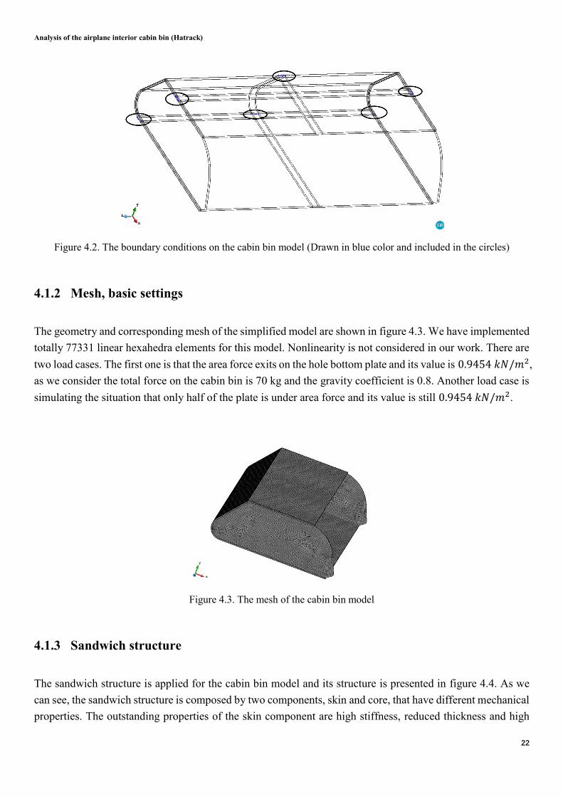
Figure 4.2. The boundary conditions on the cabin bin model (Drawn in blue color and included in the circles)

4.1.2 Mesh, basic settings

The geometry and corresponding mesh of the simplified model are shown in figure 4.3. We have implemented

totally 77331 linear hexahedra elements for this model. Nonlinearity is not considered in our work. There are

two load cases. The first one is that the area force exits on the hole bottom plate and its value is 0.9454 𝑘𝑁/𝑚2,

as we consider the total force on the cabin bin is 70 kg and the gravity coefficient is 0.8. Another load case is

simulating the situation that only half of the plate is under area force and its value is still 0.9454 𝑘𝑁/𝑚2.

Figure 4.3. The mesh of the cabin bin model

4.1.3 Sandwich structure

The sandwich structure is applied for the cabin bin model and its structure is presented in figure 4.4. As we

can see, the sandwich structure is composed by two components, skin and core, that have different mechanical

properties. The outstanding properties of the skin component are high stiffness, reduced thickness and high


23

strength. Relatively, the core of the sandwich structure is made of material with much lighter weight and much

lower stiffness. The typical example of the core is the honeycomb structure that will be implemented in the

following part related to the multiscale analysis. However, for the honeycomb structure, since there are lots

of empty spaces, the stresses on the core will be very large, which requires the material with high stiffness and

high strength. The benefits making the sandwich structure attractive for aircraft industry are:

i) They are much lighter.

ii) They are highly stiff and strong.

Figure 4.4. The sandwich structure

The size of the sandwich structure is shown in table 4.2.

Size of the sandwich

structure

CORE (mm) SKIN (mm)

6 1

Table 4.2. The size of the sandwich structure

4.2 Analysis considering isotropic materials

4.2.1 Materials

The materials used for the cabin bin in this part are a quasi-isotropic glass fiber prepreg manufactured by Gurit:

PF811-G231-32, and a foam made by BASF: Divinycell F50. The information about these two materials is

shown in table 4.3. For the glass fiber, even though it is quasi-isotropic, it will be regarded as isotropic in this

work to facilitate the simulations. The tension strength and compression strength of Divinycell F50 are

1.9 𝑀𝑃𝑎 and −0.6 𝑀𝑃𝑎 [15]. For the glass fiber PF811-G231-32, its strength under 21 𝐶𝑜 is 400 𝑀𝑃𝑎 [16].

Description Material standard Material Manufacturer Remark

CORE Divinycell F50 BASF Foam

SKIN ABS5047-42 PF811-G231-32 Gurit Glass fiber prepreg

Table 4.3. The information of the materials for the core and skin parts

Table 4.4 shows the material properties of the core and skin parts of the sandwich structure. The materials are

considered as isotropic materials.

Material properties Young's Modulus (MPa) Poisson Ratio

CORE 40 0.32

SKIN 24000 0.27

Table 4.4. The material properties of the core and skin parts

SKIN

CORE

SKIN


24

4.2.2 Results of load case 1

In load case 1, the whole bottom plate is under area force whose value is 0.9454 𝑘𝑁/𝑚2. In figure 4.5 we

can see the load case 1.

Figure 4.5. The load case 1

Displacement field

Figure 4.6 shows the displacement field of the cabin bin. The unit of the displacement field is 𝑚𝑚. From this

result, we can find that the displacements of the bottom plate are much larger compared to other parts’

displacements. The maximum displacement happens on the middle of the front edge of the bottom plate,

whose value is −7.2948 𝑚𝑚.Since the area force, boundary conditions and the structure are all symmetric,

the displacement field is consequently symmetric.

Figure 4.6. The displacement field of the cabin bin under load case 1

Principal Stress field

For the stress field on the cabin bin, the stress concentration phenomenon will be ignored in order to get the


25

accurate maximum stress and this procedure is conducted through the MIN and MAX functions in the

postprocess of GiD, which can give us the real maximum and minimum values. The unit of the stress field is

𝑀𝑃𝑎.

i. Plate area

Skin

Figure 4.7 shows the S11 principal tension stress field on the plate. The stress field on the upside plate is

uniform and small. However, on the bottom plate the stress field becomes much more complicated. For the

inside skin of the bottom plate, the large stresses arise on the area near the boundary condition and two sides.

The result is different for the outer skin of the bottom plate, since we can notice that the areas with large

stresses are the complements of the inside skin’s large stresses areas. On the area of the outer skin of the

bottom plate where the boundary condition has been applied, the maximum S11 stress appears. On this area,

we need to take more attention to avoid the fractures. The maximum S11 principal tension stress is

15.554 𝑀𝑃𝑎.

Figure 4.7. The S11 principal stress field on the skins of plates under load case 1

For the S33 principal compression stress, the result is presented in Figure 4.8. As we can see, on the upside

plate and the inside skin of the bottom plate, the S33 stresses are very small. For the outer skin of the bottom

plate, small S33 stresses are appearing on the most areas. However, around the area near the boundary

condition, the S33 stresses become much larger. The maximum S33 stress is −41.822 𝑀𝑃𝑎 and its absolute

value is also larger than the maximum S11 stress.

As we can see, the maximum S11 and S33 stresses on the skins of the plates are both lower than the stress

threshold of the glass fiber, which is 400 𝑀𝑃𝑎.


26

Figure 4.8. The S33 principal stress field on the skins of plates under load case 1

Core

The S11 principal tension stress field on the cores of the plates is shown in figure 4.9. As we can see, because

of the special sandwich structure and the different mechanical properties applied on, the skin part has

undertaken much larger stresses. As a result, the core of the structure can be made of much lighter materials

with high stiffness, causing the reduction of weight and cost. Like the situation of the skins, on the upside core

the S11 stresses are small. The areas with large S11 stresses include the area around the bottom boundary

condition and the corners of the front side of the bottom core. The maximum S11 stress is 0.08534 𝑀𝑃𝑎.

Another phenomenon is that the S11 stresses on the area where the bottom boundary condition has been

applied are smallest, meaning the S33 stresses will be largest on this area.

Figure 4.9. The S11 principal stress field on the cores of plates under load case 1

Figure 4.10 shows the S33 principal compression stress field on the cores of the plates. The S33 stresses are

still very small on the upside core. The maximum S33 stress happens on the area where we apply the bottom

boundary condition and its value is −0.15684 𝑀𝑃𝑎.

As we can see, the maximum S11 and S33 stresses on the cores of the plates are both lower than the stress

thresholds of the foam material, which are 1.9 𝑀𝑃𝑎 for the tension strength and −0.6 𝑀𝑃𝑎 for the

compression strength.


27

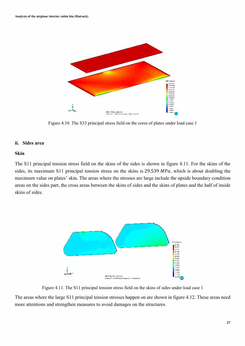
Figure 4.10. The S33 principal stress field on the cores of plates under load case 1

ii. Sides area

Skin

The S11 principal tension stress field on the skins of the sides is shown in figure 4.11. For the skins of the

sides, its maximum S11 principal tension stress on the skins is 29.539 𝑀𝑃𝑎, which is about doubling the

maximum value on plates’ skin. The areas where the stresses are large include the upside boundary condition

areas on the sides part, the cross areas between the skins of sides and the skins of plates and the half of inside

skins of sides.

Figure 4.11. The S11 principal tension stress field on the skins of sides under load case 1

The areas where the large S11 principal tension stresses happen on are shown in figure 4.12. These areas need

more attentions and strengthen measures to avoid damages on the structures.


28

Figure 4.12. The large S11 principal tension stresses on the skins of sides under load case 1

Figure 4.13 shows the S33 principal compression stress field on the skins of the sides of the cabin bin. The

maximum value is −51.369 𝑀𝑃𝑎 and its absolute value is larger than the maximum S11 principal tension

stress. Most areas of the sides are under small compression stresses, except some areas like the cross area

between the skins of plates and sides.

Figure 4.13. The S33 principal compression stress field on the skins of sides under load case 1

Figure 4.14 shows the cross areas between the upside skin of the bottom plate and the skins of two sides,

where the S33 stresses are large.

As we can see, the maximum S11 and S33 stresses on the skins of the sides are both lower than the stress



29

Figure 4.14. The large S33 principal compression stresses on the skins of sides under load case 1

Core

The S11 principal tension stress field on the cores of the sides is shown in figure 4.15. It can be seen that large

S11 stresses happen on the areas near the cross areas between the cores of sides and bottom plate and these

areas are drawn in red color. The maximum S11 stress is 0.15557 𝑀𝑃𝑎. On other areas, the stresses are small.

Figure 4.15. The S11 principal compression stress field on the cores of sides under load case 1

Figure 4.16 has shown the S33 principal compression stress field on the cores of the sides. From figure 3.1

we can find that the S33 stresses are very small on the most areas of the cores. The large S33 stresses are

showing on the cross area between the cores of the sides and the bottom plate. The maximum S33 stress can

be found on the bottom faces of the cores. The maximum S33 stress is −0.45437 𝑀𝑃𝑎.

As we can see, the maximum S11 and S33 stresses on the cores of the sides are both lower than the stress




30


The large S33 principal compression stresses on the cores of sides is shown in figure 4.17.

Figure 4.17. The large S33 principal compression stresses on the cores of sides under load case 1

iii. Back area

Skin

Figure 4.18 shows the S11 principal tension stress field on the skins of back part when we apply the load case

1. As we can see, the S11 stresses are large on the areas near the bottom boundary condition area where the

maximum S11 stress is arising on. On other areas of the back part, the stresses have much smaller values.

Figure 4.18. The S11 principal tension stress field on the skins of back part under load case 1


31

Figure 4.19 shows that where the large S11 principal tension stresses have occurred and the maximum value

is 19.905 𝑀𝑃𝑎.

Figure 4.19. The large S11 principal tension stresses on the skins of back part under load case 1

In figure 4.20 we can see the S33 principal compression stress field on the skins of the back part. Like the

situation of the S11 stress field, on the most areas of the back part, the stresses are small. However, because

of the boundary condition that we have applied, the S11 stresses near the bottom boundary condition are much

larger and this area is where we should be care of.

Figure 4.20. The S33 principal compression stress field on the skins of back part under load case 1

On the bottom boundary condition area of the outer skin, we can find the maximum S33 stress. The maximum

value is −25.016 𝑀𝑃𝑎 and it is also the area where the maximum S11 stress happens. Figure 4.21 shows the

bottom boundary condition area on the skins of the back part where the S33 stresses are large.

As we can see, the maximum S11 and S33 stresses on the skins of back part are both lower than the stress



32

Figure 4.21. The large S33 principal compression stresses on the skins of back part under load case 1

Core

The S11 principal tension stress field on the core of the back part is shown in figure 4.22. On the bottom

boundary condition area, the values of the S11 stresses are negative. However, the S11 stresses are large on

the areas around the boundary condition area and the maximum S11 stress is 0.14193 𝑀𝑃𝑎. On other areas

of the core, the S11 stresses are small.

Figure 4.22. The S11 principal tension stress field on the cores of back part under load case 1

The S33 principal compression stress field on the core of the back part is shown in figure 4.23. From this

figure we can see that except the bottom boundary condition area, the S33 stresses are very small on the most

areas of the core. The large S33 stresses appear on the bottom boundary condition area and the its maximum

value is −0.16354 𝑀𝑃𝑎.

As we can see, the maximum S11 and S33 stresses on the cores of the back part are both lower than the stress




33

Figure 4.23. The S33 principal compression stress field on the cores of back part under load case 1

Bending stress field

For the beading stress field, the discussions will only focus on the bottom plate, which has undertaken the

bending force mostly. The directions of the bending stresses Sxx and Szz are shown in the left part of figure

4.24.

Skin

The Sxx bending stress field on the skins of the plates is shown in figure 4.24. As we can see, the stresses on

the skins of the upside plate are small. On the inside skin of the bottom plate, the tension stresses are large on

the area near the bottom boundary condition, drawn in dark red. For the outer skin of the bottom plate, on the

area around the bottom boundary condition, we can find large compression stresses. The maximum tension

and compression stresses are both happening on the bottom boundary condition area. The maximum tension

stress is 6.6227 𝑀𝑃𝑎 and the maximum compression stress is −24.285 𝑀𝑃𝑎.

Figure 4.24. The Sxx bending stress field on the skins of plates under load case 1

Figure 4.25 shows the tension and compression distribution of the Sxx stress field on the skins of the plates.

The areas without showing the stresses are under tension stresses while other areas are representing the


34

compression stresses areas.

Figure 4.25. The tension and compression stresses’ distribution of Sxx stresses on the skins of plates

The Szz bending stress field on the skins of the plates is shown in figure 4.26. Like the situation of the Sxx

bending stress field, on the skins of the upside plate, the Szz bending stresses are small. On the inside skin of

the bottom plate, the areas where the tension stresses are large are the area near the bottom boundary condition

and the two front corners. The compression stresses are large on the middle and front area of the inside skin.

For the outer skin of the bottom plate, the Szz stress field is the complementation of the stress field of inside

skin. The area having large compression stresses, the bottom boundary condition area and the two front corners,

are the area where the tension stresses are large on the inside skin. The maximum Szz tension stress appears

on the right corner of the inside skin and its value is 6.8125 𝑀𝑃𝑎. The maximum Szz compression stress can

be found on the bottom boundary condition area and its value is −17.306 𝑀𝑃𝑎.

The tension and compression stresses’ distribution of Szz stresses is shown in figure 4.27. The tension stresses

have been represented by the areas without showing the stresses.

Figure 4.26. The Szz bending stress field on the skins of plates under load case 1


35

Figure 4.27. The tension and compression stresses’ distribution of Szz stresses on the skins of plates

Core

The Sxx bending stress field on the cores of the plates is shown in figure 4.28. As we can see, the stress

distribution on the cores are similar to the stress distribution on the skins. Near the bottom boundary condition

area, the tension stresses are large. The bottom boundary condition area itself has large compression stresses.

On the two sides of the core of the bottom plate, the tension stresses are large. The maximum tension and

maximum compression stresses are both happening on the bottom boundary condition area and their values

are 0.029449 𝑀𝑃𝑎 and −0.084093 𝑀𝑃𝑎, which are very small compared the stresses on the skins.

Figure 4.28. The Sxx bending stress field on the cores of plates under load case 1

Figure 4.29 has shown the tension and compression stresses’ distribution of the Sxx stresses on the cores.

Figure 4.29. The tension and compression stresses’ distribution of Sxx stresses on the cores of plates

From figure 4.30 we can find that the distribution of the Szz stresses is similar to the situation of the Sxx stress


36

field. The bottom boundary condition area has large compression stresses while the tension stresses are also

large near this area. On the two sides of the bottom, the large tension stresses can be found. The maximum

tension and maximum compression stresses are both appearing on the bottom condition area. The maximum

tension stress is 0.025938 𝑀𝑃𝑎 and the maximum compression stress is −0.081009 𝑀𝑃𝑎. They are also

very small.

The tension and compression stresses’ distribution of the Szz stresses is shown in figure 4.31.

Figure 4.30. The Szz bending stress field on the cores of plates under load case 1

Figure 4.31. The tension and compression stresses’ distribution of Szz stresses on the cores of plates


37

4.2.3 Results of load case 2

The difference between two load cases is that the area force is applied only on half of the bottom plate in load

case 2. And its value is still 0.9454 𝑘𝑁/𝑚2 and we can see this load case in figure 4.32. The load case 2 might

be a critical situation for the structure since a torque force will be applied on the structure.

Figure 4.32. The load case 2

Displacement field

The displacement field of the cabin bin under load case 2 is shown in figure 4.33. In load case 1, the

displacement field of the cabin bin is symmetric. However, in load case 2, since the area force is no longer

symmetric, the displacement field on left half part of the structure becomes larger than the right half part. And

its maximum displacement is −3.5022 𝑚𝑚 now, which is about half of the maximum displacement value in

load case 1. The maximum displacement still happens on the front edge of the bottom plate but it moves left

compared to load case 1.

Figure 4.33. The displacement field of cabin bin under load case 2


38


The stress concentration will be also ignored in this part.

i. Plate area

Skin

Figure 4.34 shows the S11 principal tension stress field on the skins of the plates under load case 2. Similar

to the situation of displacement field, the stress field becomes nonsymmetric and its values on the left part of

the plates are larger. The areas where the S11 stresses are large are on the skins of the bottom plate. As figure

has shown, these areas are the left side of the inside skin, the area near the bottom boundary condition on the

inside skin and left part of the outer skin. On the skins of the upside plate, the S11 stresses are small like the

situation of load case 1. However, the maximum S11 principal tension stress in load case 2 is 8.4327 𝑀𝑃𝑎

and this is smaller than its value in load case 1.

Figure 4.34. The S11 principal tension stress field on the skins of plates under load case 2

The S33 principal compression stress field on the skins of the plates is shown in figure 4.35. In load case 2,

the maximum S33 principal stress still happens on the bottom boundary condition area and its value is

−22.582 𝑀𝑃𝑎. On other parts of the plates, the S33 stresses are not large.


39

Figure 4.35. The S33 principal compression stress field on the skins of plates under load case 2

As we can see, the maximum S11 and S33 stresses on the skins of plates are both lower than the stress


Core

The S11 principal tension stress field on the cores of the plates is shown in figure 4.36. As we can see, the

S11 stress field becomes nonsymmetric. The right and front corners of the bottom plate have large S11 stresses

under the load case 1. However, in load case 2, the areas with large S11 stresses only have the area around the

bottom boundary condition and the left and front corner. The maximum S11 stress is 0.06014 𝑀𝑃𝑎 and it has

decreased compared to load case 1.


The S33 principal compression stress field on the cores of the plates is shown in figure 4.37. The S33 stress

distribution is similar to the S11 stress distribution. The left and front corner of the bottom core and the

boundary condition area have large S33 stresses. The maximum S33 stress is −0.10184 𝑀𝑃𝑎 and its value

becomes smaller compared to load case 1.


40


As we can see, the maximum S11 and S33 stresses on the cores of the plates are both lower than the stress



ii. Sides area

Skin

Figure 4.38 shows the S11 principal tension stress field on the skins of the sides. Taking a comparison between

load case 1 and load case 2, we can find that the areas where the stresses are large become much smaller in

load case 2. The upside boundary condition area on the outer skin of left side and the cross areas between the

skins of left side and plates have large stresses. The maximum S11 stress value is 24.789 𝑀𝑃𝑎, which is

smaller than it in load case 1.


Figure 4.39 shows the areas where the S11 principal tension stresses are large and they are all on the left side,

which is the difference between load case 1 and load case 2. Now, combining the results from two load cases,

we are able to implement corresponding reinforcements on those areas having large stresses as shown.

Figure 4.39. The large S11 principal tension stress areas on the skins of sides under load case 2

The S33 principal compression stress field on the skins of the sides is shown in figure 4.40. On the most areas,


41

the stresses are small. However, as we can see above, the cross areas between the skins of plates and the skins

of sides could have large stresses and this still applies here. The maximum S33 principal stress appears on the

cross area between the inside skin of the bottom plate and the inside skin of the left side. Its value is

−31.083 𝑀𝑃𝑎 and this is smaller than the load case 1.

Figure 4.40. The S33 principal compression stress field on the skins of sides under load case 2


Figure 4.41 shows the area having large S33 principal compression stresses.

As we can see, the maximum S11 and S33 stresses on the skins of sides are both lower than the stress threshold

of the glass fiber, which is 400 𝑀𝑃𝑎.

Core

The S11 principal tension stress field on the cores of the sides is shown in figure 4.42. The large S11 stresses

are appearing on the cross area between the cores of left side and the cores of the bottom plate. And the

maximum S11 stress is 0.11124 𝑀𝑃𝑎, which has also decreased.

The S33 principal compression stress field on the cores of the sides is shown in figure 4.43. From this figure

we can find that the S33 stresses are small on the most areas of the cores of the sides. And the large S33

stresses can be found on the bottom face of the left side and the maximum S33 stress is −0.32372 𝑀𝑃𝑎,

whose absolute value also decreases compared to the load case 1.


42

Figure 4.42. The S11 principal tension stress field on the cores of sides under load case 2


The figure 4.44 has shown the large S33 principal compression stress on the cores of the sides.

Figure 4.44. The large S33 principal compression stress on the cores of sides under load case 2

As we can see, the maximum S11 and S33 stresses on the cores of the sides are both lower than the stress



43


iii. Back area

Skin

From figure 4.45 we can see the S11 principal tension stress field on the skins of the back part under load case

2. The S11 stresses near the bottom boundary condition area are large. And the maximum S11 principal stress

is 10.633 𝑀𝑃𝑎, which is smaller than the load case 1.


The bottom boundary condition area with large S11 principal tension stresses is shown in figure 4.46. Unlike

the results in load case 1 that the stress field is symmetric, the S11 stresses are comparatively larger on the left

part.

Figure 4.46. The large S11 principal tension stresses on the skins of back part under load case 2

Figure 4.47 shows the S33 principal stress field on the skins of the back part under load case 2. Except the

bottom boundary condition area, other areas of the skins of the back part are under small S33 principal

compression stresses. And the maximum value in this situation is −13.795 𝑀𝑃𝑎 and its absolute value is

smaller compared to load case 1.


44




Core

In figure 4.48, the S11 principal tension stress field on the core of the back part can be seen. On the curved part

of the core, the stresses are large, especially on the area around the bottom boundary condition. The maximum

S11 stress has decreased to 0.077295 𝑀𝑃𝑎 in load case 2. The S11 stresses are small on the flat part of the

core.

Figure 4.49 shows the S33 principal compression stress field on the core of the back part. Unlike the situation

of S11 stress field that the S11 stresses are large on the curved part of the core, the area with large S33 stresses

is only the bottom boundary condition area. The maximum S33 stress is −0.10382 𝑀𝑃𝑎, also becomes

smaller.

Figure 4.48. The S11 principal tension stress field on the core of back part under load case 2


45

Figure 4.49. The S33 principal compression stress field on the core of back part under load case 2

As we can see, the maximum S11 and S33 stresses on the cores of back part are both lower than the stress




Skin

The Sxx bending stress field on the skins of the plates under load case 2 is shown in figure 4.50. Comparing

the corresponding stress field in load case 1, we can find that Sxx stresses are smaller in load case 2, although

the torque force exits in this part. The stresses on the skins of upside plate are very small. On the two sides of

the skin of the bottom plate, the tension stresses are no longer that large. The large tension stresses happen on

the bottom boundary condition area on the inside skin. For the outer skin, the areas around the bottom

boundary condition have large compression stresses. And we can find the maximum tension and maximum

compression stresses on the bottom boundary condition area. The maximum tension stress is 3.4309 𝑀𝑃𝑎,

which has decreased compared to load case 1. The maximum compression stress is −12.715 𝑀𝑃𝑎 and its

absolute value has also decreased.


Figure 4.51 has shown the tension and compression stresses’ distribution of the Sxx stresses on the skins of

the plate.


46

Figure 4.51. The tension and compression stresses’ distribution of Sxx stresses on the skins of plates

The Szz bending stress field on the skins of the plates under load case 2 has been shown in figure 4.52. Same

as the situation of Sxx stress field, the Szz stress field is no longer symmetric under load case 2. On the skins

of the upside plate, the Szz stresses are very small. The left side of the inside skin of the bottom plate has large

tension stresses. The large tension stresses also happen on the bottom boundary condition area on the inside

skin and the most of the left part of the outer skin. On other areas of the skins, the compression stresses can

be found. On the inside skin, the large compression stresses occur on the corresponding area where the tension

stresses are large on the outer skin. It is same for the large compression stresses distribution on the outer skin

and we can find them on the bottom boundary condition area and the left side. The maximum Szz tension

stress is 4.2785 𝑀𝑃𝑎 and the maximum Szz compression stress is −9.7646 𝑀𝑃𝑎. These values also have

decreased compared to load case 1.



47

Figure 4.53. The tension and compression stresses’ distribution of Szz stresses on the skins of plates

Figure 4.53 shows the tension and compression stresses’ distribution of the Szz stresses on the skins under

load case 2.

Core

The Sxx bending stress field on the cores of the plates under load case 2 has been shown in figure 4.54. The

distribution of the Sxx stresses on the cores is similar to the situation of skins. Except that on the bottom

boundary condition area we can only find the large compression stresses, although the large tension stresses

appear on the areas near the bottom boundary condition. The maximum tension stress is 0.016763 𝑀𝑃𝑎 and

the maximum compression stress is −0.054337 𝑀𝑃𝑎.

The tension and compression stresses’ distribution of Sxx stresses is shown in figure 4.55.


Figure 4.55. The tension and compression stresses’ distribution of Sxx stresses on the cores of plates


48

The Szz bending stress field on the cores of the plates under load case 2 is shown in figure 4.56. As we can

see, the distribution of the Szz stresses is similar to the case of Sxx stresses. The maximum tension stress

happens on the left side of the core and its value is 0.015108 𝑀𝑃𝑎. The maximum compression stress is

−0.052908 𝑀𝑃𝑎 and it can be found on the bottom boundary condition area.

The Szz tension and compression stresses’ distribution is shown in figure 4.57.


Figure 4.57. The tension and compression stresses’ distribution of Szz stresses on the cores of plates

4.2.4 Conclusions

From above contents that we have discussed, we can get some useful conclusions to guide our design and

optimization of the structure:

i) The load case 1 is more dangerous than the load case 2, since the principal stresses S11 and principal

stress S33 on every part of the structure under load case 1 is larger than the load case 2. Consequently, the

following part about multiscale analysis will only focus on the load case 1.

ii) The areas that have large principal stresses S11 and principal stress S33 should be taken into attention to

implement measurements to reduce the stress concentrations produced by the supports and the crossing

between bottom plate and sides. Like replacing the materials on those areas to the materials with higher


49

stiffness. These areas include the upside boundary condition area on the sides, the bottom boundary condition

area on the bottom plate and the back part, and the cross areas between the sides and bottom plates. On other

areas of the cabin bin, the stresses are not large.

iii) Thanks to the outstanding mechanical properties of sandwich structure, the core part of the structure has

undertaken very small stresses and the skins are under much larger stress field, meaning that we can build

lighter structure with higher stiffness.

iv) The maximum S11 and S33 stresses are both found in load case 1. On the skins, the maximum S11

principal tension stress is found on the upside boundary condition area of the sides and its value is

29.539 𝑀𝑃𝑎. For the maximum S33 principal compression stress, it happens on the cross area between the

inside skin of bottom plate and the inside skins of two sides, whose value is −51.369 𝑀𝑃𝑎.

On the cores, the maximum S11 principal tension stress happens on the cross area between the core of bottom

plate and the core of two sides and its value is 0.15557 𝑀𝑃𝑎. The maximum S33 principal compression stress

is appearing on the bottom face of two sides and the value is −0.45437 𝑀𝑃𝑎.

By comparing the maximum stresses on the skins and cores with the materials used, we can find the

performance of the cabin bin with isotropic materials. Since the strength of the glass fiber is 400 𝑀𝑃𝑎, the

stresses on the skins of cabin bin under two load cases are both lower than the its stress threshold. And for the

foam core, its tension strength is 1.9 𝑀𝑃𝑎 and compression stress is −0.6 𝑀𝑃𝑎. Therefore, the stresses on the

cores of the cabin bin are also below the stress threshold of the foam cores.


50

4.3 Analysis with a multiscale procedure

4.3.1 Material, RVEs

In this part, the sandwich structure is still used for our model. The skin part corresponds to RVE_01 and the

core part is the material represented by RVE_02. The RVE_02 is a honeycomb structure. The two RVEs and

corresponding microstructures are shown in figure 4.58. The RVE_01 has three components: Fiber on X

direction, Fiber on Y direction and matrix. For the RVE_02, there is only the matrix that has been implemented.

In RVE_01, the fibers on X and Y directions are woven ramie fibers and the matrix is epoxy matrix. The

honeycomb structure (RVE_02) is manufactured from high temperature resistant aramid paper formed into a

honeycomb structure, and coated with a phenolic resin [17]. The tension strength and compression strength of

epoxy are 85 𝑀𝑃𝑎 and −112 𝑀𝑃𝑎 [18]. For the ramie fiber, its tension strength is about 560 𝑀𝑃𝑎 [19]. The

strength of the honeycomb structure as a simple material is 2.4 𝑀𝑃𝑎 [17].

Figure 4.58. The RVE models for the skin and core together with the real microstructures (Upside: RVE_01, down:

RVE_02)

Table 4.5 shows the material properties of the fibers and matrix used for RVE_01. The materials implemented

here are all isotropic and nonlinearity is considered. Shear modulus are set to be zero in this part.

Material properties of the components

Components Young Modulus (MPa) Poisson Ratio

Fiber_X (Woven ramie) 24000 0.01

Fiber_Y (Woven ramie) 24000 0.01

Matrix (Epoxy) 3500 0.25

Table 4.5. Material properties for the components of RVE_01


51

With above components, the material properties of the RVE_01 as a simple material are shown in table 4.6.

The RVE_01 becomes anisotropic as the table 4.6 has presented. The material properties are obtained from

the initial analysis of the RVE in which it has loads from different space directions in order to get the elastic

stiffness tensor of the material, which is required by the FEM to evaluate the structure stiffness. Then, the

anisotropic material parameters that define the composites can be obtained from the material stiffness tensor.

Those are the ones shown in table 4.6 and table 4.8 for RVE_01 and RVE_02.

The RVE_01 Material properties

Young Modulus (MPa) Exx Eyy Ezz

11750.02 11822.1 9907.3

Shear Modulus (MPa) Gxy Gxz Gyz

5239.05 4750.49 4733.67

Poisson Ratio

Pxy Pyx Pxz

0.0804 0.0799 0.1115

Pzx Pyz Pzy

0.1323 0.11 0.1313

Table 4.6. The material properties of RVE_01 as a simple material

In table 4.6, we can see that Exx and Eyy are very close, this is because that the ramie fibers’ distributions on

X and Y directions are very similar. The slight difference is caused by that the RVE is developed from an

image of the real material in which the fibers on X and Y directions are not exactly same. On the other hand,

since the ramie fibers are not oriented in Z direction, Ezz is smaller than Exx and Eyy. For the Shear Modulus,

the similar situation is found that Gxz and Gyz are very close but not exactly same while Gxy is larger.

In this part, we have implemented the honeycomb structure to the core parts, which has huge empty spaces.

This leads to the increases of the stresses on the core parts, even though we will see that the stresses on the

cores shown in macroscopic are still very small. This difference is caused by the computation procedure that

the stresses on the macroscopic scale are the results of the volumetric average of the microscopic stresses in

the RVE. As a result, the material with high stiffness and high strength is used to avoid the damage on the

core parts.

The material property of the matrix of the RVE_02 is shown in table 4.7. The matrix is anisotropic for the

Shear Modulus. The Shear Modulus on XZ direction is set to be 12000 MPa and on other directions it will be

zero.

Material properties of the components

Components Young Modulus (MPa) Shear Modulus (XZ, MPa) Poisson Ratio

Matrix (Aramid paper) 18000 12000 0.3

Table 4.7. Material properties for the matrix of RVE_02

The material properties of RVE_02 as a simple material has been shown in table 4.7. We can see that the

values of the Young Modulus and Shear Modulus on all directions are much smaller compared to RVE_01.

For the Poisson Ratio, the Pxy and Pyx are larger than 0.5, which seems wrong since the Poisson Ratio should

be less than 0.5. However, this makes sense for the honeycomb structure, as it will decrease its volume

considerably when the forces are applied. For other materials like metal, the volume is assumed to be

incompressible, which limits the maximum value of Poisson Ratio to 0.5. Therefore, because of the failure of


52

the incompressibility assumption for the honeycomb structure, the limitation of Poisson Ratio is no longer

appropriate in this case. In PLCd, the limitation of the Poisson Ratio exits in the setting section of materials.

Consequently, Pxy and Pyx are both set as 0.45 to satisfy the request.

The RVE_02 Material properties

Young Modulus (MPa) Exx Eyy Ezz

34.88 35.10 138.31

Shear Modulus (MPa) Gxy Gxz Gyz

10.20 41.06 30.54

Poisson Ratio

Pxy Pyx Pxz

0.5348 0.5313 0.3000

Pzx Pyz Pzy

0.0756 0.3000 0.0761

Table 4.8. The material properties of RVE_02 as a simple material

From table 4.8 we can also find that the Young’s Modulus on Z direction is much larger compared to the other

two directions. This result is reasonable since the stiffness on Z direction is larger than the other two, caused

by that the honeycomb cells are oriented on Z direction and there are larger deformations on X and Y directions.

4.3.2 Results

Displacement field

The displacement field of the cabin bin under load case 1, calculated by the multiscale analysis, is shown in

figure 4.59. Since we have applied different materials in this part, the maximum displacement happening on

the middle of the front edge of the bottom plate becomes larger. From the figure we can see that the value of

maximum displacement is −12.691 𝑚𝑚. And except the bottom plate, other parts of the cabin bin have much

smaller displacements. Because of the symmetricities existing in the area force, structure and boundary

conditions, the displacement field is also symmetric.

Figure 4.59. The displacement field of the cabin bin under load case 1


53

Microscopic procedure

The numerical result of the displacement on Y direction of the microscopic procedure is shown in figure 4.60.

The RVEs chosen in this part are representing the skin and core of the upside plate. Their positions are shown

in figure 4.59 with a fork mark on the upside plate.

Figure 4.60. The displacement solutions on the chosen RVEs of microscopic procedure


The indexes chosen for the discussion about stress field will be S11 principal tension stress and S33 principal

compression stress. In order to show the differences on the stress field, caused by the use of the eco-composites,

the stresses in following part will be compared to the load case 1 in part 4.2.2. Therefore, the descriptions

about the increasing and decreasing of the stresses are all based on the comparison between following part

and the load case 1 in part 4.2.2.

Because of the stress concentration phenomenon, a normal numerical issue, we will see that some elements

have much larger stresses compared to other areas where this problem is not exiting. Therefore, following

discussions about the stress field will ignore this phenomenon and the maximum stress pointed out below will

be considered under this condition.

Another issue is that since on the macroscopic scale the stresses are calculated as the volumetric average

values with respect to the RVEs and the RVE_02 model has very large empty spaces, the stresses on the

RVE_02 are actually much larger than the macroscopic stresses on the core parts of the cabin bin. For the

RVE_01, the real stresses on the fibers and matrix are close to the average values.

Last, even though the macroscopic stresses on the cores are not the actual stresses, it still has meanings from

an average perspective. The macroscopic stresses can point out where the stresses are large and then we can

choose the elements on these areas to show the real stresses. In following part, since the real stresses on cores

are much larger than the macroscopic stresses, the microscopic stresses on the cores will be shown. And the

strength of the honeycomb structure is given as a simple material, therefore it is necessary to compare the

macroscopic stresses with the strength to check the safety of the cores of cabin bin.


54

i. Plates area

Skin

The S11 principal tension stress field of the skin of cabin bin has been shown in figure 4.61. The S11 stresses

are not large on the most areas of the plates’ skin, especially on the upside plate. The areas having large S11

stresses include the boundary condition area and the two sides of the inside skin of the bottom plate. Without

the consideration of stress concentration phenomenon, the maximum S11 stress on the skins of plates is

13.823 𝑀𝑃𝑎, which has decreased.


The S33 principal compression stress field on the skins of the plates is shown in figure 4.62. Similar to the

situation of the S11 stress field, the S33 stresses on the most areas of the plates’ skins are small. However, on

the boundary condition area where the maximum S33 compression stress appears, the absolute value of the

maximum S33 stress is about three times than the maximum S11 stress. The maximum S33 compression stress

is −34.798 𝑀𝑃𝑎 and its absolute value has decreased. Combining the truth that the S11 also becomes smaller,

we can conclude that the application of the eco-composites has helped the structure to decrease the stress field.

And this conclusion will be confirmed by following discussions.


As we can see, the maximum S11 and S33 stresses on the skins of plates are both lower than the stress

thresholds of the epoxy and ramie fibers.


55

Core

The chosen elements to show the microscopic S11 and S33 stresses are shown in figure 4.63. They are

element 60734, element 38672 and element 24353.

Figure 4.63. The S11 principal tension stress field on the cores of plates under load case 1

The S11 principal tension stress field on the cores of the plates is shown in figure 4.63. Compared to the skins,

the S11 stresses on the cores are much smaller. The areas where the S11 stresses are large on the cores are

similar to the situation of skins. The S11 stresses are large on the boundary condition area of the bottom core

and the bottom core’s front corners. And the maximum S11 stress is 0.13217 𝑀𝑃𝑎, which becomes larger.

The microscopic S11 stress fields on the RVEs of element 60734, element 38672 and element 24353 are

shown in figure 4.64. On the RVE of element 60734, the maximum S11 stress is 35.15 𝑀𝑃𝑎. The maximum

S11 stress on the RVE of element 38672 is close to the RVE of element 60734 and its value is 35.043 𝑀𝑃𝑎.

The maximum S11 stress on the RVE of element 24353 is 71.751 𝑀𝑃𝑎, about doubling the maximum S11

stresses on the other two RVEs.


56

Figure 4.64. The microscopic S11 stresses on the RVE_02 of element 60732, element 24353 and element 38672

(Upside: element 60732, down left: 24353, down right: 38672)

The S33 principal tension stress field on the cores of the plates is shown in figure 4.64. The large S33 stresses

appear on the same areas where the S11 stresses are large. And the maximum S33 compression stress is

−0.34478 𝑀𝑃𝑎 and this value is about doubling the value in the load case 1 in part 4.2.2.

Figure 4.65. The S33 principal compression stress field on the cores of plates under load case 1


57

Figure 4.66. The microscopic S11 stresses on the RVE_02 of element 60732, element 24353 and element 38672

(Upside: element 60732, down left: 24353, down right: 38672)

In figure 4.66, we can see the microscopic S33 stress fields on the RVEs of chosen elements. The element

60734 RVE’s maximum S33 stress is much smaller compared to other two element and the value is

−16.774 𝑀𝑃𝑎. On the RVE of element 24353, the S33 compression stress is also very large and the maximum

S33 stress is −66.914 𝑀𝑃𝑎. For the RVE of element 38672, its maximum S33 stress is −63.779 𝑀𝑃𝑎, which

is also very large.

As we can see, the maximum S11 and S33 stresses on the cores of plates are both lower than the stress

thresholds of the honeycomb structure as a simple material, which is 2.4 𝑀𝑃𝑎.

ii. Sides area

Skin

The S11 principal tension stress field on the skins of the sides is shown in figure 4.67. From this figure we

can see that the S11 stresses are large on the upside boundary condition area of the outer skin and the cross

areas between the skins of plates and sides. Except on these areas, the S11 stresses are small. The maximum

S11 stress is 27.028 𝑀𝑃𝑎, which is smaller than it in the load case 1 in part 4.2.2.


Figure 4.68 shows where the S11 principal tension stresses are large.


58

Figure 4.68. The large S33 principal compression stresses on the skins of sides under load case 1 (Up: cross areas

between skins of the plates and sides, down: the upside boundary condition area on the outer skin of sides)

The S33 principal compression stress field on the skins of the sides is shown in figure 4.69. The maximum

S33 stress is −40.873 𝑀𝑃𝑎 and it happens on the cross areas between the inside skin of bottom plate and the

skins of sides. Comparing this maximum S33 stress with the corresponding value in the load case 1 in part

4.2.2, whose value is −51.369 𝑀𝑃𝑎, its absolute value has decreased. As we know from above discussion,

on this area, the S11 stress is also very large. Therefore, this area is the most dangerous area on the skins of

the sides under the load case 1.


The large S33 principal compression stress area is shown in figure 4.70.

As we can see, the maximum S11 and S33 stresses on the skins of sides are both lower than the stress



59


Core

Figure 4.71. The S11 principal tension stress field on the cores of sides under load case 1

Figure 4.71 shows the S11 principal tension stress field on the cores of the sides. Like the situation we have

discussed about the plates, the core of the sandwich structure has undertaken much smaller stresses compared

to skins. The large S11 stresses are appearing on the areas around the cross areas between the cores of sides

and plates. The maximum S11 stress is 0.42298 𝑀𝑃𝑎. On other areas on the cores of the sides, the S11 stresses

are small.

The chosen element for showing the microscopic S11 stress is element 3025, whose location is shown in figure

4.71. The microscopic S11 principal tension stress field on the RVE of element 3025 is shown in figure 4.72

and its maximum S11 stress is 123.94 𝑀𝑃𝑎.


60

Figure 4.72. The microscopic S11 stresses on the RVE_02 of element 3025

The S33 principal compression stress field on the cores of the sides is shown in figure 4.73. The large S33

stresses appear on the bottom faces of the cores. The maximum S33 stresses appear on the bottom faces of the

cores and its value is −0.99005 𝑀𝑃𝑎. The element 3092 has been chosen to show the microscopic S33 stress

and its location is shown in figure 4.73.


As we can see from figure 4.74, the microscopic S33 stresses on the RVE of element 3092 are very large. The

maximum S33 stress is −198.48 𝑀𝑃𝑎.



61

As we can see, the maximum S11 and S33 stresses on the cores of sides are both lower than the stress


iii. Back area

Skin

The S11 principal tension stress field on the skins of the back part is shown in figure 4.75. Like the above

results that we have seen, on the most areas of the skins, the S11 stresses are small. However, the area around

the boundary condition area on the bottom of the back part has large stresses. The maximum S11 stress is

15.586 𝑀𝑃𝑎 and it is smaller than the its corresponding value in the load case 1 in part 4.2.2.


The S33 principal compression stress field on the skins of the back part has been shown in figure 4.76. Similar

to what we have discussed about the S11 stress field, the large S33 stresses are also appearing around the area

where the bottom boundary condition has been applied on. And on other areas of the back part, the S33 stresses

are not large. The value of the maximum S33 compression stress is −22.277 𝑀𝑃𝑎. As a comparison, the

maximum S33 stress on the skins of the back part in the load case 1 in part 4.2.2 is −25.016 𝑀𝑃𝑎. Therefore,

the eco-composites help the structure to decrease its stress field on the skins of the back part.





62

Core

The S11 principal tension stress field on the core of the back part is shown in figure 4.77. Around the bottom

boundary condition area on the back part, the S11 stresses are large. And this area with large S11 stresses is

shown in red color. On other areas of the core, the S11 stresses are not large. The maximum S11 stress is

0.17882 𝑀𝑃𝑎. Figure 4.77 also gives the locations of the element 53437 and element 38571 that we will use

to show the microscopic stresses.

Figure 4.77. The S11 principal tension stress field on the core of back part under load case 1

Figure 4.78 shows the microscopic S11 principal tension stress field on the RVE of element 53437. The

maximum S11 stress is 103.75 𝑀𝑃𝑎.


The S33 principal compression stress field on the core of the back part is shown in figure 4.79. The maximum

S33 stress happens on the bottom boundary condition area on the core and its value is −0.29068 𝑀𝑃𝑎.


63

Figure 4.79. The S33 principal compression stress field on the core of back part under load case 1

The microscopic S33 principal tension stress field on the RVE of element 38571 is shown in figure 4.80. The

maximum S33 stress is −124.29 𝑀𝑃𝑎.


As we can see, the maximum S11 and S33 stresses on the cores of back part are both lower than the stress



The bending stress field will only be discussed on the bottom plate, as the bending effects are much clearer

on this region. The directions of the bending Stresses Sxx and Syy have already been shown in above figure

4.24.

Skin

The Sxx bending stress field on the skins of the plates is shown in figure 4.81. The skins on the upside plate

have small stresses. The large tension stresses occur on the bottom condition area on the inside skin. For the


64

compression stresses, we can also find the large stresses on the bottom condition area and the areas around it.

The RVEs are chosen from this area to show the Sxx stresses and their numbers are 24102 and 24598, which

are respectively located on the bottom boundary condition area on the inside skin and the outer skin. Figure

4.81 also shows the positions of these two elements.


Figure 4.82 shows the microscopic Sxx stress field on the RVEs of element 24102 and element 24598. From

this this figure we can see that the matrix has undertaken larger stresses than the fibers. As we discussed above,

the microscopic stresses are close to the macroscopic stresses in RVE_01. For the RVE of element 24102, the

maximum Sxx tension stress and compression stress both happen on the matrix and their values are

7.0552 𝑀𝑃𝑎 and −11.873 𝑀𝑃𝑎. The situation is same for the RVE of element 24598. The maximum Sxx

tension and compression stresses are also found on the matrix and their values are 9.858 𝑀𝑃𝑎 and

−12.255 𝑀𝑃𝑎.


65

Figure 4.82. The microscopic Sxx bending stress field on the RVE_01 of element 24102 and element 24598 (Up:

24102, down:24598, left: matrix, right: fibers)

The Szz bending stress field on the skins of the plates is shown in figure 4.83. For the inside skin of the bottom

plate, the bottom boundary condition area and the two front corners possess large tension stresses. On the front

and middle area, we can find the large compression stresses. As we can see, the situation of the outer skin of

the bottom plate is converse. The chosen RVEs are from above areas on the skins of the bottom plate. Figure

4.83 also shows the positions of element 25162, element 38780, element 38707 and element 39259, which are

used to show the microscopic Sxx and Szz bending stresses.


The microscopic Szz stress fields on the RVEs of element 24102 and element 24598 are shown in figure 4.84,

representing bottom boundary condition area. We can see that the stresses on the matrix are much larger than

the stresses on the fibers. The maximum Szz tension and compression stresses on the RVE of element 24102

are 3.4119 𝑀𝑃𝑎 and −5.0959 𝑀𝑃𝑎 . For the RVE of element 24598, the maximum Szz tension and

compression stresses are 4.7173 𝑀𝑃𝑎 and −5.2403 𝑀𝑃𝑎.


66

Figure 4.84. The microscopic Szz bending stress field on the RVE_01 of element 24102 and element 24598 (Up:


The Szz stress fields on the RVEs of element 25162 and element 33780, located on the front corners on the

skins of the bottom plate, are shown in figure 4.85. As it has been presented, the stresses on the matrix are still

larger than the stresses on the fibers. The stresses are uniform on the most parts, including the matrix and the

fibers. The maximum Szz tension and compression stresses on the RVE of element 25162 are 25.279 𝑀𝑃𝑎

and −28.702 𝑀𝑃𝑎. For the RVE of element 33780, the maximum Szz tension and compression stresses are

13.746 𝑀𝑃𝑎 and −24.296 𝑀𝑃𝑎.


67



The Szz stress fields on the RVEs of element 38707 and element 39259 is shown in figure 4.86 and they

represent the front and middle area of the skins of the bottom plate. As we can see, the stresses on following

RVEs are not uniform like we have seen above. For the element 38707, located on the inside skin, the matrix

and the fibers are all under compression stresses and the maximum Szz compression stress in its RVE is

−10.32 𝑀𝑃𝑎 and it appears on the matrix. Conversely, for the RVE of element 39259 which is on the outer

skin, the stresses are tension stresses and the maximum tension stress in its RVE is also found on the matrix

with the value 9.6566 𝑀𝑃𝑎.



Core


68

The Sxx bending stress field on the cores of the plates is shown in figure 4.87. On the bottom boundary

condition area, the large compression stresses can be found. For the large tension stresses, they are

happening on the area near the bottom boundary condition and the two front corners of the bottom core. As

we have discussed above about the principal stresses, the stresses on the cores are much smaller than the

stresses on the skins. The results are same for the bending stresses in this part. However, since the

honeycomb structure has very large empty spaces and the macroscopic stresses have been derived from the

volumetric average of the stresses in the RVE, the real stresses will be much larger on the honeycomb

structure. Therefore, the material used to manufacture the honeycomb cores should possess high stiffness

and high strength.


The Sxx stress field on the RVE of element 60734 (Shown in figure 4.63), located on the left side of the

bottom core, is shown in figure 4.88. On this RVE, the stresses are much larger than the macroscopic stresses

on the cores. This result proves that the existence of the empty spaces in the RVE leads to the huge increases

of the microscopic stresses compared to the macroscopic stresses. The maximum Sxx tension and compression

stresses in the RVE of element 60734 are 35.15 𝑀𝑃𝑎 and −15.047 𝑀𝑃𝑎.

Figure 4.88. The microscopic Sxx bending stress field on the RVE_02 of element 60734

The RVEs in figure 4.89 are selected from the bottom boundary condition area and this figure has shown the

Sxx stress field on these RVEs. The elements are 38672 and 24353 (Shown in figure 4.63). As we can see,


69

both RVEs have large compression stresses. The RVE of element 24353 also has very large tension stresses.

The maximum Sxx tension and compression stresses in the RVE of element 38672 are 13.058 𝑀𝑃𝑎 and

−38.425 𝑀𝑃𝑎 . For the RVE of element 24353, the maximum tension and compression stresses are

30.094 𝑀𝑃𝑎 and −33.717 𝑀𝑃𝑎.

Figure 4.89. The microscopic Sxx bending stress field on the RVE_02 of element 38672 and element 24353 (Left:

38672, right: 24353)

The Szz bending stress field on the cores of the plates is shown in figure 4.90. The bottom boundary condition

area, the two front corners and the front and middle area of the bottom core have both large tension and

compression stresses.


Figure 4.91 shows the Szz bending stress field on the RVE of element 60734 (Shown in figure 4.63) selected

from the left front corner of the bottom core. The maximum Szz tension and compression stresses are

12.814 𝑀𝑃𝑎 and −16.774 𝑀𝑃𝑎. The position of element 38980 is also shown in figure 4.91.


70

Figure 4.91. The microscopic Szz bending stress field on the RVE_02 of element 60735

The Szz bending stress field on the element 38672 and element 24353 (Shown in figure 4.63) has been shown

in figure 4.92 and these two elements are located on the bottom boundary condition area. The compression

stresses are large on these two RVEs and the tension stresses on the RVE of element 38672 are also large. The

maximum Szz tension and compression stresses on the RVE of element 38672 are 20.818 𝑀𝑃𝑎 and

−30.696 𝑀𝑃𝑎. For the RVE of element 24353, the maximum Szz tension and compression stresses are

9.9575 𝑀𝑃𝑎 and −19.641 𝑀𝑃𝑎.

Figure 4.92. The microscopic Szz bending stress field on the RVE_02 of element 38672 and element 24353 (Left:

38672, right: 24353)

Another area where the Szz stresses are large is the front and middle area of the bottom core. Therefore, the

element 38980 has been selected and the Szz stress field on the RVE of this element is shown in figure 4.93.

As we can see, this RVE is under compression stresses. And the maximum Szz compression stress is

−6.061 𝑀𝑃𝑎.


71

Figure 4.93. The microscopic Szz bending stress field on the RVE_02 of element 38980

Comparison

Table 4.9 shows that the application of the eco-composites has decreased the S11 and S33 stresses on the skins

of the structure compared to the former design with isotropic materials.

The maximum S11 and S33 stresses on different skin parts of the cabin bin

Skins Isotropic materials

(S11, MPa)

Eco-composites

(S11, MPa)

Isotropic materials

(S33, MPa)

Eco-composites

(S33, MPa)

Skin of the plates 15.554 13.823 −41.822 -34.798

Skin of the sides 29.539 27.028 -51.369 -40.873

Skin of the back part 19.905 15.586 -25.016 -22.277

Table 4.9. The maximum S11 and S33 stresses on different skin parts of the cabin bin

Table 4.10 has shown the comparison between the S11 and S33 stresses on the cores of the structure under

the situations that the eco-composites are implemented or not and this comparison is based on the average

perspective. From table we can see that the application of the eco-composites will increases the S11 and S33

stresses on the core parts of the cabin bin even from an average perspective. Actually, the stresses on the cores

will increase significantly, leading to the demand to use highly stiff and highly strong materials for the cores.

The maximum S11 and S33 stresses on different core parts of the cabin bin

Cores Isotropic materials

(S11, MPa)

Eco-composites

(S11, MPa)

Isotropic materials

(S33, MPa)

Eco-composites

(S33, MPa)

Core of the plates 0.08534 0.13217 -0.15684 -0.34478

Core of the sides 0.15557 0.42298 -0.45437 -0.99005

Core of the back part 0.14193 0.17882 -0.16354 -0.29068

Table 4.10. The maximum S11 and S33 stresses on different core parts of the cabin bin


72

4.3.3 Conclusions

i) The application of eco-composites has helped the structure to decrease its stress field on the skins of the

structure. However, the stresses on the core parts will become much larger than the situation of using isotropic

materials.

ii) The areas where the large S11 and S33 stresses have appeared on need reinforcements to protect the

structure from being damaged.

iii) Because of the large empty spaces of the eco-honeycomb RVE model and the computation procedure

that the macroscopic stresses are calculated by taking the volumetric average of the microscopic stresses in

the RVE, the stresses on the honeycomb core are actually much larger than the stresses shown in macroscopic

scale. As a result, it is needed to analyze the performance of the RVE in order to study the real stresses on the

cores when the average stresses on the macroscopic scale have not provided this information.

iv) The stresses on the cabin bin with isotropic materials or eco-composites are all lower than the stress

thresholds of corresponding materials.

Conclusions

73

5 Conclusions

Before the simulation works, the theories of FEM, multiscale homogenization and 𝐹𝐸2 homogenization

procedure have been discussed. Through the presentations of these theories, the formulations and working

flow behind PLCd code become clear, which is necessary for conducting this work. Then the following work

has successfully simulated the simple supported beam and the cabin bin, under different load cases using the

isotropic materials and eco-composites. And the analysis of the cabin bin made of eco-composites is conducted

by using the multiscale analysis procedure. There are some conclusions given by the results.

First, from the beam model we can see that the solutions are convergent and the errors will be very small if

we use enough elements. And using quadratic elements will give lower errors compared to using linear

elements. Another conclusion is that the stress concentration will lead to errors on the area where it happens.

Therefore, the MIN and MAX functions of GiD should be used to get real maximum stresses.

Then, for the simulation of the cabin bin with isotropic materials, the results show that the load case 1

(completely loaded cabin bin) is more dangerous, even though the load case 2 (load applied only to half of the

cabin bin) will add a torque force on the structure. And the areas where the stresses are large are upside

boundary condition area on the sides, bottom boundary condition area on the bottom plate and the back part,

and the cross areas between the sides and bottom plates. In order to reduce the stress concentrations, we can

take measurements like replacing the materials on these area with stiffer materials. The conclusion about the

sandwich structure is that the core parts have undertaken much smaller stresses, which allows us to use the

lighter material for the cores to decrease the weight of the structure.

For the simulation of the cabin bin with eco-composites using multiscale analysis procedure, the first

conclusion is that the application of the eco-composites will decrease the stress field on the skins of the

structure. For the core parts, the actual stresses on the cores will increase because of the large empty spaces in

the honeycomb structure. However, the macroscopic stresses on the cores will keep very small since the

computation of the macroscopic stresses is taking the volumetric average of the microscopic stresses in the

RVE. For the increases of stresses on the core parts after using the eco-composites, we can avoid the damage

by using the material with high stiffness and high strength. As a result, the benefit of sandwich structure that

it will help the structure to decrease its weight can be achieved safely.

The last conclusion is that the stresses on the cabin bin with isotropic materials or eco-composites are all lower

than the stress thresholds of corresponding materials.

References

74

6 References

[1] Bachmann, J.; Yi, X.; Gong, H.; Martinez, X.; Tserpes, K.; Ramon, E.; Paris, C.; Moreira, P.; Fang, Z.; Li,

Y.; et al. Outlook on ecologically improved composites for aviation interior and secondary structures. CEAS

Aeronaut. J. 2018, 9, 533-543.

[2] PLCd-Manual. Non-linear thermomachanic finite element code, developed at CIMNE, 1991-present.

(https://web.cimne.upc.edu/users/plcd/)

[3] C. Truesdell; R. Toupin. The Classical Field Theories, Handbuch der Physik Ⅲ/Ⅰ. Springer-Verlag,

Berlin,1960.

[4] Oller, S.; Neamtu, L.; & Oñate, E. Una generalización de la teoría de mezclas clásica para el tratamiento

de compuestos en serie/paralelo. Congreso Nacional de Materiales Compuestos, pp. 433-438, 1995.

[5] Oñate, E.; Neamtu, L.; & Oller, S. Un modelo constitutivo para el análisis por el “MEF” para materiales

compuestos. In J. Güemes & C. Navarro (Eds.), Materiales Compuestos '97, pp. 206-211, 1997.

[6] Otero, F; Oller, S; & Martínez, X. Multiscale Computational Homogenization: Review and Proposal of a

New Enhanced-First-Order Method. Volume 25, Issue 2, pp. 479-505, 2018.

[7] Ostoja-Starzewski, M. Microstructural Randomness Versus Representative Volume Element in Thermo-

mechanics. Journal of Applied Mechanics, 69(1):25-35, 2002.

[8] Oñate, E. Introduction to the finite element method. CIMNE, Lectures for the master program of

computational mechanics, 2008

[9] Otero, F. Multiscale Numerical Modelling of Microstructured Reinforced Composites, PhD thesis, Escola

Tecnica Superior d'Enginyers de Camins, Canals i Ports de Barcelona, Universidad Politécnica de Catalunya,

2015. Advisor: Oller, S; Martínez, X.

[10] R. Hill. A self-consistent mechanics of composite materials. Journal of the Mechanics and Physics of

Solids, 13(4):213-222, 1965.

[11] J. Mandel. Plasticite Classique Et Viscoplasticite. International Centre for Mechanical Sciences, Courses

and lectures, Springer-Verlag, Udine, 1971.

[12] Frederic Feyel. Multiscale 𝐹𝐸2 elastoviscoplastic analysis of composite structures, Computational

Materials Science, 16:344-354, 1999.

[13] Frederic Feyel. A multilevel finite element method (𝐹𝐸2) to describe the response of highly non-linear

structures using generalized continua, Comput. Methods Appl. Mech. Engrg, 192:3233–3244, 2003.

[14] Otero, F; Martínez, X; & Oller, S. An efficient multi-scale method for non-linear analysis of composite

structures. Composite Structure, Volume 131, pp.707-719, 2015

[15] BASF Corporation. Divinycell F: properties data. (https://aerospace.basf.com/)

https://web.cimne.upc.edu/users/plcd/

References

75

[16] Gruit Group. General Datasheet: PF 811. (https://www.gurit.com/)

[17] Hexcel Corporation. HexWeb® A1 and A10: product data. (http://www.hexcel.com/)

[18] Simmons (Mouldings) Ltd. Epoxy resin. (http://www.epoxyworktops.com/)

[19] Doshi Group. Ramie fiber. (http://www.doshi-group.com/)

https://www.gurit.com/

http://www.hexcel.com/

http://www.epoxyworktops.com/

http://www.doshi-group.com/

numerical analysis of interior aircraft structures made of de

Documents