numerical analysis of dipole sound source around high speed trains

Redistri

Numerical analysis of dipole sound source around highspeed trains

Takehisa Takaishi,a) Akio Sagawa, Kiyoshi Nagakura, and Tatsuo MaedaRailway Technical Research Institute, Shiga 521-0013, Japan

~Received 23 January 2002; revised 23 March 2002; accepted 23 March 2002!

As the maximum speed of high speed trains increases, the effect of aeroacoustic noise on the soundlevel on the ground becomes increasingly important. In this paper, the distribution of dipole soundsources at the bogie section of high speed trains is predicted numerically. The three-dimensionalunsteady flow around a train is solved by the large eddy simulation technique. The time history ofvortices shows that unstable shear layer separation at the leading edge of the bogie section shedsvortices periodically. These vortices travel downstream while growing to finally impinge upon thetrailing edge of the section. The wavelength of sound produced by these vortices is large comparedto the representative length of the bogie section, so that the source region can be regarded asacoustically compact. Thus a compact Green’s function adapted to the shape can be used todetermine the sound. By coupling the instantaneous flow properties with the compact Green’sfunction, the distribution of dipole sources is obtained. The results reveal a strong dipole source atthe trailing edge of the bogie section where the shape changes greatly and the variation of flow withtime is also great. On the other hand, the bottom of the bogie section where the shape does notchange, or the leading edge and boundary layer where the variation of flow with time is small,cannot generate a strong dipole source. ©2002 Acoustical Society of America.@DOI: 10.1121/1.1480833#

PACS numbers: 43.28.Ra, 43.50.Nm, 43.50.Lj@MSH#

ed21es

nnt

eeisli

oic

ea

oiepan

utaoiisthire

ofindel.

enn isAn-gehedaterf, theeights by

a-ssure

the

nd,er

ateri-he

ec.’s

’s

I. INTRODUCTION

In 1964 high speed trains called ‘‘Shinkansen’’ startcommercial service in Japan with a maximum speed ofkm/h ~131 miles/h!. Since then Japan Railway compani~formerly Japanese National Railways! have progressivelyraised the speed of Shinkansen trains. The environmequality standards established by the Japanese governmequire that the peak noise level must not exceed 75 dB~A!.Because rolling noise was dominant in the early days, whand rails have been profiled periodically. Then spark nogenerated by the contact breaks between overheadequipment and pantograph, became dominant. This nwas reduced when all pantographs were connected elecally to avoid contact loss. The introduction of these msures permitted the maximum speed of Shinkansen toincreased to 270 km/h. Then, however, aeroacoustic nfrom upper parts of the train became dominant. The largsound source was the aeroacoustic noise from pantograThis was reduced by installing large pantograph coversspecially designed low-noise pantographs.1 Now that thenoise from all there sources has been reduced, aeroaconoise from lower parts of the train have become an imporproblem. Since the dominant frequency of aeroacoustic nis far lower than that of other sources, such as rolling noit cannot totally be reduced by noise barriers. Therefore,reduction of aeroacoustic noise is one of the key requments for further increases in train speed.

a!Electronic mail: [email protected]

J. Acoust. Soc. Am. 111 (6), June 2002 0001-4966/2002/111(6)/2

bution subject to ASA license or copyright; see http://acousticalsociety.org/

0

talre-

lse,nesetri--

besesths.d

sticntsee,e-

In order to reduce aeroacoustic noise several kindswind tunnel tests have been performed at the Maibara WTunnel, which has an excellent low background noise levExperimental results with a 1/5 scale model Shinkans2

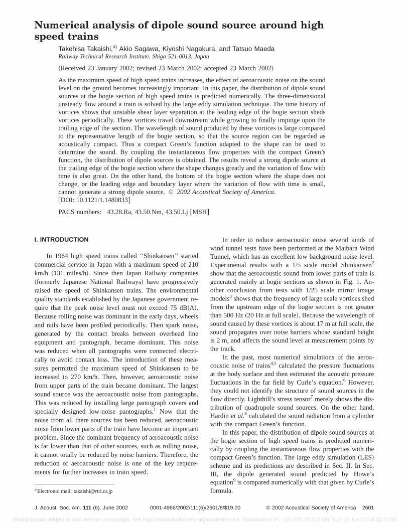
show that the aeroacoustic sound from lower parts of traigenerated mainly at bogie sections as shown in Fig. 1.other conclusion from tests with 1/25 scale mirror imamodels3 shows that the frequency of large scale vortices sfrom the upstream edge of the bogie section is not grethan 500 Hz~20 Hz at full scale!. Because the wavelength osound caused by these vortices is about 17 m at full scalesound propagates over noise barriers whose standard his 2 m, and affects the sound level at measurement pointthe track.

In the past, most numerical simulations of the aerocoustic noise of trains4,5 calculated the pressure fluctuationat the body surface and then estimated the acoustic presfluctuations in the far field by Curle’s equation.6 However,they could not identify the structure of sound sources inflow directly. Lighthill’s stress tensor7 merely shows the dis-tribution of quadrupole sound sources. On the other haHardin et al.8 calculated the sound radiation from a cylindwith the compact Green’s function.

In this paper, the distribution of dipole sound sourcesthe bogie section of high speed trains is predicted numcally by coupling the instantaneous flow properties with tcompact Green’s function. The large eddy simulation~LES!scheme and its predictions are described in Sec. II. In SIII, the dipole generated sound predicted by Howeequation9 is compared numerically with that given by Curleformula.

2601601/8/$19.00 © 2002 Acoustical Society of America

content/terms. Download to IP: 131.230.73.202 On: Sun, 21 Dec 2014 13:27:55

tnr

em

30lla

blk

rtemariffu, r

de

y–

by

dy

on-n inure-

ncyrs,ion.nd

s aus

nd

talnal

nehe

nsa-l r

toelsthe

Redistri

II. UNSTEADY FLOW SIMULATION BY LES

A. Formation

The large eddy simulation~LES! technique directlycomputes energy-containing eddies that are larger thangrid scale, and the effect of the smallest scales of turbuleis modeled through a subgrid scale stress term. To sepathe large from the small scales, a physical variablef is fil-tered and defined as a space-averaged variable. Sincgoverning equations are discretized by the finite volumethod, a top-hat filter is provided implicitly,

f~y!5E f~y8!H~y,y8!dy8, ~1!

whereH is the top-hat filter function satisfying

H~y,y8!51/V for y8Pcomputational cell

50 otherwise ~2!

andV is the volume of the computational cell.Because the train speed considered in this study is

km/h ~83.3 m/s! and its Mach number is sufficiently smarelative to unity, the flow around trains can be regardedincompressible. If the filtering operation~1! is applied to theequations of continuity and momentum for incompressiflow, the filtered governing equations for the grid scale tathe form

]ui

]yi50, ~3!

]ui

]t1uj

]ui

]yj52

1

r

] p

]yi1

]

]yi~2t i j 12nSi j !, ~4!

whereSi j is the grid scale rate of strain tensor

Si j 51

2 S ]ui

]yj1

]uj

]yiD , ~5!

andt i j is the subgrid scale stress tensor

t i j 5uiuj2ui u j . ~6!

The governing equations for the grid scale are conveto a system of algebraic equations by the finite volumethod with unstructured cells. The convection termsdiscretized by second-order upwind methods, and the dsion terms by second-order central-differenced methodsspectively.

The time derivative is discretized using the second-oraccurate backward differences:

Thus]f/]t5F(f) becomes

FIG. 1. Contour of the sound pressure level of 1/5 scale model Shinkathat is tested in the wind tunnel~Ref. 2!. The sound pressure level is mesured by using a sound concentrating microphone with a paraboloidaflector whose diameter is 1 m.

2602 J. Acoust. Soc. Am., Vol. 111, No. 6, June 2002


heceate

thee

0

s

ee

dee-

e-

r

f i5 43 fn2 1

3 fn211 23 DtF~f i !. ~7!

The pressure-implicit with splitting of operators methods10

are used for pressure–velocity coupling.The subgrid scale stress tensort i j is simplified by the

eddy viscosity model

t i j 522neSi j , ~8!

where the eddy viscosity is modeled by the SmagorinskLilly hypothesis

ne5Ls2A Si j Si j . ~9!

Ls is the mixing length for subgrid scales and is computedusing

Ls5min~0.42d, CsV1/3!, ~10!

where d is the distance to the closest wall. In this stuSmagorinsky constantCs is fixed as 0.1.

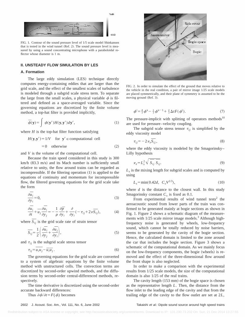
From experimental results of wind tunnel tests2 theaeroacoustic sound from lower parts of the train was cfirmed to be generated mainly at bogie sections as showFig. 1. Figure 2 shows a schematic diagram of the measments with 1/25 scale mirror image models.3 Although high-frequency noise is generated by wheels, low-frequesound, which cannot be totally reduced by noise barrieseems to be generated by the cavity of the bogie sectHence, the calculated domain is limited to the zone arouthe car that includes the bogie section. Figure 3 showschematic of the computational domain. As we mainly focon the low-frequency components, the bogie~wheels! is re-moved and the effect of the three-dimensional flow arouthe front shape is also neglected.

In order to make a comparison with the experimenresults from 1/25 scale models, the size of the computatiodomain is also 1/25 of the real trains.

The cavity length~153 mm! of the bogie space is choseas the representative lengthL. Then, the distance from thflow inlet to the leading edge of the cavity and that from ttrailing edge of the cavity to the flow outlet are set at 2L,

en

e-

FIG. 2. In order to simulate the effect of the ground that moves relativethe vehicle in the real condition, a pair of mirror image 1/25 scale modare placed symmetrically, and their plane of symmetry is assumed to bemoving ground~Ref. 3!.

Takaishi et al.: Dipole sound source around high speed trains


ttodai

is

lertkta/hhee-room-

gec

thll

rtifccdrt

eesroll

d inres-

atex-

w

nd

Redistri

respectively. The space between the ground and the boof the vehicle is set as 16 mm. The center of the leading eof the cavity is set as the origin of the coordinates, trrunning~main flow! direction as thex axis, side direction asthey axis, and vertical direction as thez axis. The number ofgrid points inside the bogie section is 51331321. The num-ber of cells included in the whole computational domain661 350.

The stochastic components of the flow at the inboundaries are accounted for by superposing random pebations on individual velocity components. In order to mathe conditions of simulation coincide with the experimentest conditions, the mean flow velocity is set to 300 km~83.3 m/s!, and the turbulence intensity is set to 0.3%. Tzero diffusion flux condition is applied at the outlet; the vlocity gradient in the flow direction is assumed to be zeand the conditions of the outflow plane are extrapolated frwithin the domain. The no-slip condition for velocity is applied at the ground and the train surface.

As the initial condition (t50 s) for LES calculation, thetime-steady solution obtained by thek2« model is used.The physical time stepDt is set to 2.531024 s.

Unsteady flow simulation by LES is performed usinFLUENT version 5. The estimation of the dipole sound in SIII is performed by programming a shell module.

B. Results

The following discussion uses data acquired aftertime history of the drag exerted on the train becomes fuperiodic (t50.225– 0.250 s).

Figure 4 shows three-dimensional distributions of voces around a train. They are the views from the bottom otrain, and indication of the ground boundary is omitted. Eafigure shows iso-surfaces of vorticity vector in each diretion. The unstable shear layer separation at the leading eof the bogie section sheds vortices periodically. These vo

FIG. 3. Computational domain of unsteady flow around the train. Asmainly focus on the low-frequency components, the bogie~wheels! is re-moved.

J. Acoust. Soc. Am., Vol. 111, No. 6, June 2002


mgen

tur-el

.

ey

-ah-gei-

ces travel downstream while growing to finally impingupon the trailing edge of the section. Longitudinal vorticare formed along the side covers of the bogie section andup at the trailing edge.

The incompressible pressure fluctuation is expressethe logarithmic scale in the same way as for the sound psure,

pressure fluctuation level~dB!520 logA^p2&

p0,

~11!p05231025 Pa,

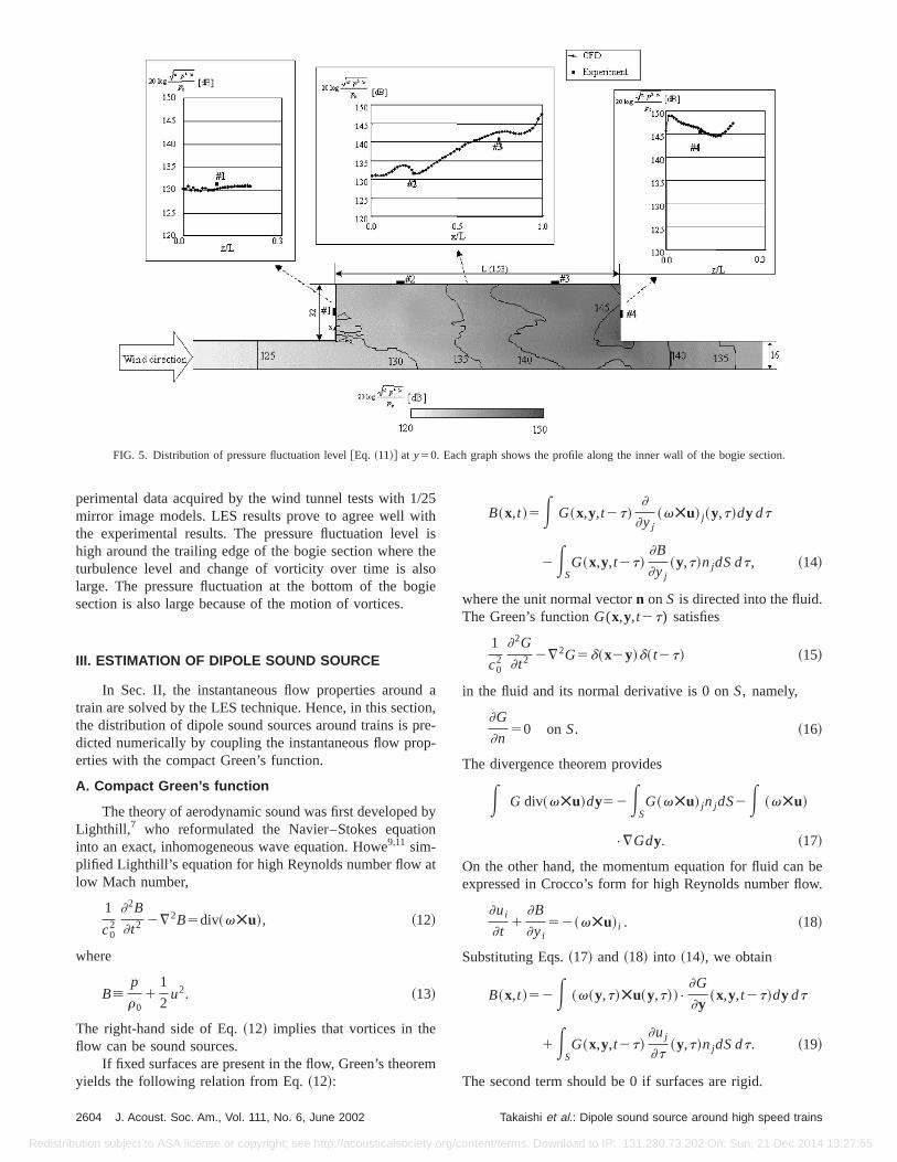
where^ & denotes time-averaged value.Figure 5 shows the distribution of pressure fluctuation

the bogie section. Point marks in each graph show the

e

FIG. 4. Iso-surface of vorticity vector:~a! x component,~b! y component,and ~c! z component. They are the views from the bottom of a train, aindication of the ground boundary is omitted.

2603Takaishi et al.: Dipole sound source around high speed trains


Redistri

FIG. 5. Distribution of pressure fluctuation level@Eq. ~11!# at y50. Each graph shows the profile along the inner wall of the bogie section.

/2ithlth

lsog

diorep

bon

t

em

bew.

perimental data acquired by the wind tunnel tests with 1mirror image models. LES results prove to agree well wthe experimental results. The pressure fluctuation levehigh around the trailing edge of the bogie section whereturbulence level and change of vorticity over time is alarge. The pressure fluctuation at the bottom of the bosection is also large because of the motion of vortices.

III. ESTIMATION OF DIPOLE SOUND SOURCE

In Sec. II, the instantaneous flow properties arountrain are solved by the LES technique. Hence, in this sectthe distribution of dipole sound sources around trains is pdicted numerically by coupling the instantaneous flow proerties with the compact Green’s function.

A. Compact Green’s function

The theory of aerodynamic sound was first developedLighthill,7 who reformulated the Navier–Stokes equatiinto an exact, inhomogeneous wave equation. Howe9,11 sim-plified Lighthill’s equation for high Reynolds number flow alow Mach number,

1

c02

]2B

]t2 2¹2B5div~vÃu!, ~12!

where

B[p

r01

1

2u2. ~13!

The right-hand side of Eq.~12! implies that vortices in theflow can be sound sources.

If fixed surfaces are present in the flow, Green’s theoryields the following relation from Eq.~12!:



5

ise

ie

an,-

-

y

B~x,t !5E G~x,y,t2t!]

]yj~vÃu! j~y,t!dy dt

2ESG~x,y,t2t!

]B

]yj~y,t!njdS dt, ~14!

where the unit normal vectorn on S is directed into the fluid.The Green’s functionG(x,y,t2t) satisfies

1

c02

]2G

]t2 2¹2G5d~x2y!d~ t2t! ~15!

in the fluid and its normal derivative is 0 onS, namely,

]G

]n50 on S. ~16!

The divergence theorem provides

E G div~vÃu!dy52ESG~vÃu! jnjdS2E ~vÃu!

•¹Gdy. ~17!

On the other hand, the momentum equation for fluid canexpressed in Crocco’s form for high Reynolds number flo

]ui

]t1

]B

]yi52~vÃu! i . ~18!

Substituting Eqs.~17! and ~18! into ~14!, we obtain

B~x,t !52E ~v~y,t!Ãu~y,t!!•]G

]y~x,y,t2t!dy dt

1ESG~x,y,t2t!

]uj

]t~y,t!njdS dt. ~19!

The second term should be 0 if surfaces are rigid.



,

nagi

neo

ical

sec-

the

dyof

hat

ro

ent

Redistri

If the observation pointx is far from the source regionEq. ~13! can be approximated as

B>pa

r0, ~20!

and the acoustic pressure fluctuation in the far field is

pa~x,t !52r0E $v~y,t!Ãu~y,t!%•]G

]y~x,y,t2t!dy dt.

~21!

If the source region is compact, the three-dimensioGreen’s function may be expanded around the source rein the form9

Gc>1

4puxudS t2t2

uxuc0

D1x•Y

4pc0uxu2]

]tdS t2t2

uxuc0

D1

1

uxuOF S 2p l

l D 2G . ~22!

In this equation,Yj denotes the velocity potential of aimaginary flow around the body that has unit speed in thjdirection at large distances from the body. This velocity ptential must satisfy Laplace’s equation

¹2Yj50 ~23!

in the fluid and also

FIG. 6. Model of dipole sound sources close to the ground. By mirsources, dipole sound sources in thex direction~a! andy direction~b! willbe doubled. In contrast, the sources in thez direction~c! will be canceled byequal and opposite image dipoles.

FIG. 7. Contours of the velocity potentialY around the train.



lon

-

]Yj~y!

]n50 ~24!

on surfaces. The Green’s function governs the acoustproperties of the system: the velocity potentialY depends onthe body shape, but does not represent a real flow. Theond term of Eq.~22!,

Gc>x"Y

4pc0uxu2]

]tdS t2t2

uxuc0

D , ~25!

represents the production of dipole sound, and is called ‘‘compact Green’s function.’’9

In the present problem, the frequency of the unsteadrag force exerted on the train by the periodic sheddingvortices is about 200 Hz. Also, the experiments confirm t

r

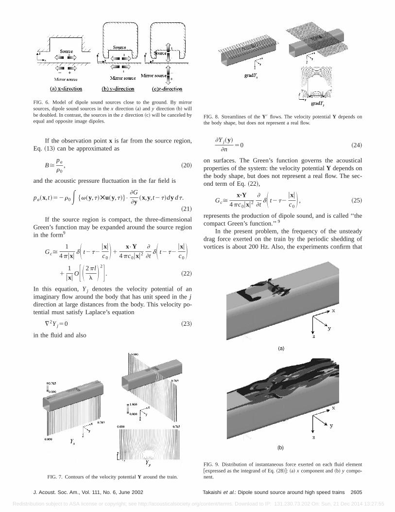
FIG. 8. Streamlines of theY8 flows. The velocity potentialY depends onthe body shape, but does not represent a real flow.

FIG. 9. Distribution of instantaneous force exerted on each fluid elem@expressed as the integrand of Eq.~28!#: ~a! x component and~b! y compo-nent.



paesth

vs

ocedt,dee

-

ine

id

ure

n.ea-the

not

f

Redistri

the frequency of large scale vortices generated by flow seration at the upstream edge of the bogie section is not grethan 500 Hz. The wavelength of sound produced by thvortices is about 0.5–2 m, which is large compared withrepresentative length of the bogie section~0.153 m!. There-fore, when the low frequency sound that propagates onoise barriers is taken into consideration, sound sourcesisfy the condition of compactness.

Dipole sound sources close to the ground can be meled as shown in Fig. 6. The effect of the ground is replaby mirror sources.12,13 By mirror sources, dipole sounsources in thex andy directions will be doubled. In contrasthe sources in thez direction will be canceled by equal anopposite image dipoles. As a result, the effective thrdimensional compact Green’s function becomes

Gc~x,y,t2t!'xjYj~y!

2pc0uxu2]d

]t S t2t2uxuc0

D , j 51,2.

~26!

Here j 51 and 2 denotes thex and y component, respectively.

Substituting Eq.~26! into Eq. ~21!, we obtain

Pa52r0xj

2pc0uxu2]

]t E ~vÃu!~y,t2uxu/c0!

•gradYjdy, j 51,2. ~27!

This is the final form of the acoustic pressure fluctuationthe far field that is produced by dipole sound sources closthe ground.

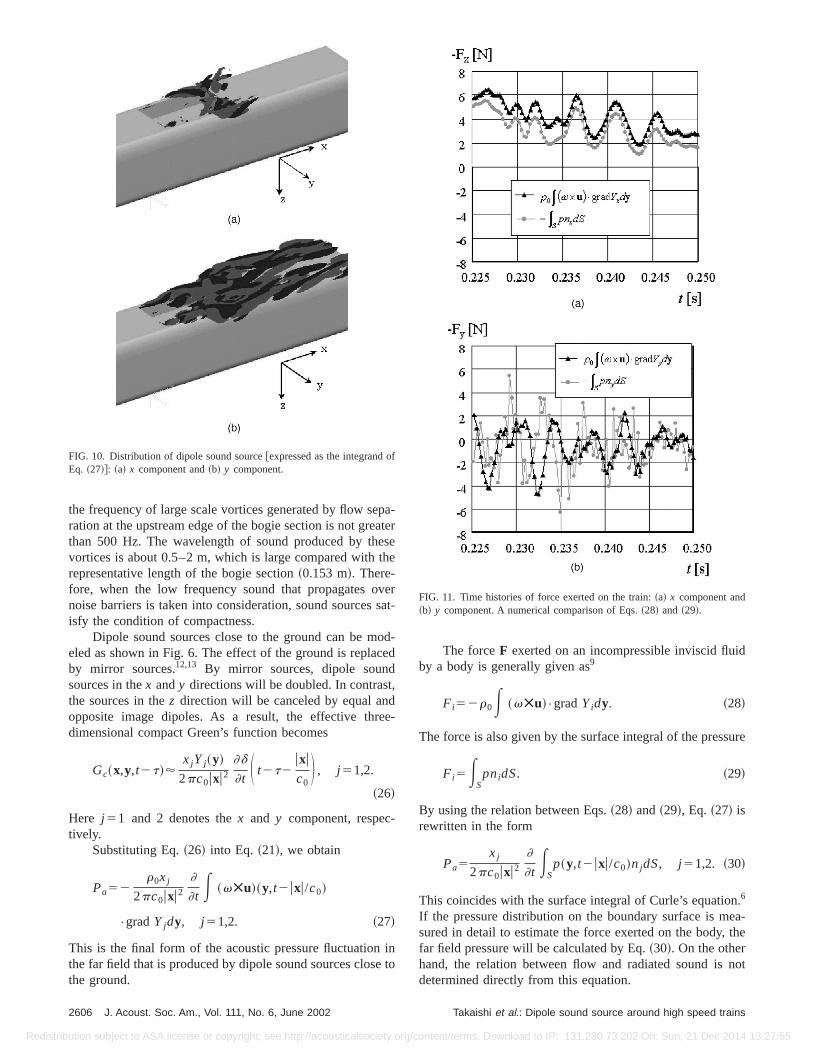
FIG. 10. Distribution of dipole sound source@expressed as the integrand oEq. ~27!#: ~a! x component and~b! y component.



a-tere

e

erat-

d-d

-

to

The forceF exerted on an incompressible inviscid fluby a body is generally given as9

Fi52r0E ~vÃu!•gradYidy. ~28!

The force is also given by the surface integral of the press

Fi5ESpnidS. ~29!

By using the relation between Eqs.~28! and~29!, Eq. ~27! isrewritten in the form

Pa5xj

2pc0uxu2]

]t ESp~y,t2uxu/c0!njdS, j 51,2. ~30!

This coincides with the surface integral of Curle’s equatio6

If the pressure distribution on the boundary surface is msured in detail to estimate the force exerted on the body,far field pressure will be calculated by Eq.~30!. On the otherhand, the relation between flow and radiated sound isdetermined directly from this equation.

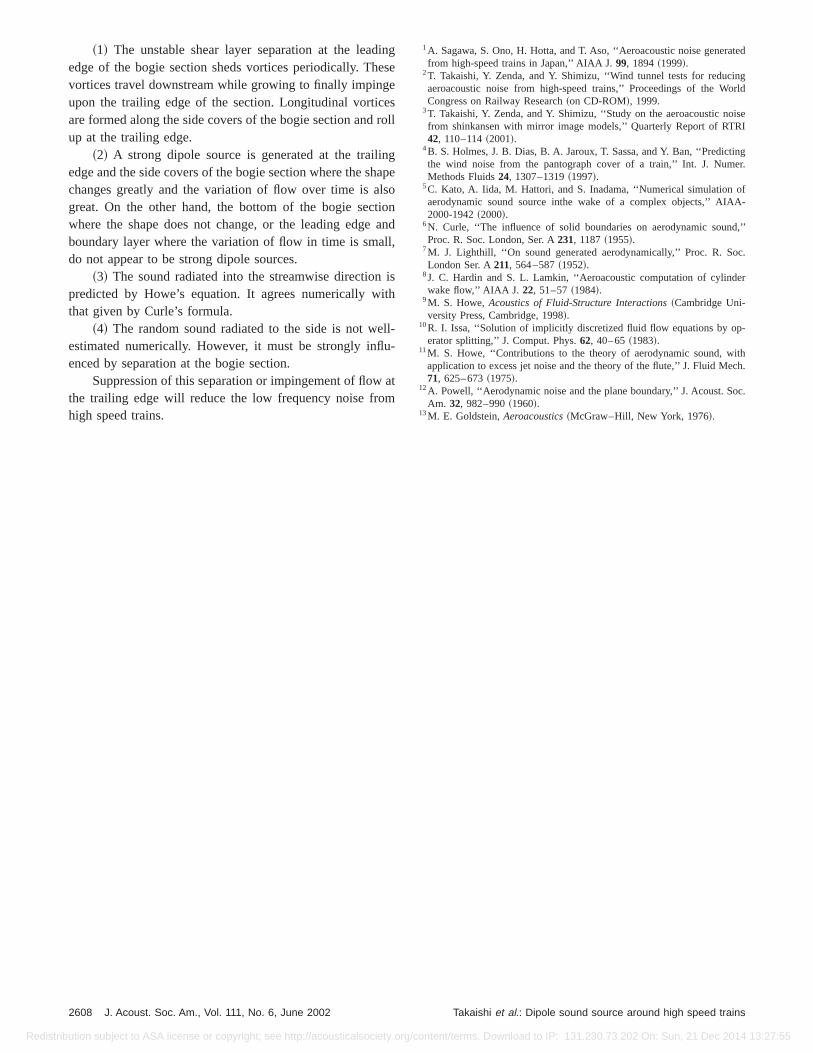
FIG. 11. Time histories of force exerted on the train:~a! x component and~b! y component. A numerical comparison of Eqs.~28! and ~29!.



m

thth

he

-

the

ndis-q.us

d of

veesea-of

nden-gien ofof

r theows.’s

andrce

ine

dif-the

ted,. In-idetheonin

on

u-theit.

theh

heesre

ua

Redistri

Howe’s method selects a Green’s function whose norderivative at the boundary surface is zero as in Eq.~16!.Then the effect of the boundary surface is included inGreen’s function and the acoustic pressure fluctuation infar field is expressed in a volume integral as Eq.~27!. SinceEq. ~27! is expressed in terms of the motion of vortices, trelation between the flow and radiated sound is explicit.

B. Results

First, Laplace’s equation~23! is solved numerically withboundary condition~24!. Figure 7 shows contours of the velocity potentialY around the train.

Figure 8 shows the streamlines of theY8 flows. In eachfigure, the velocity has unit speed in thex andy directions at

FIG. 12. Time histories of the sound pressure atuxu54.42 m: ~a! x compo-nent and~b! y component. A numerical comparison between Curle’s eqtion ~30! and Howe’s equation~27!.



al

ee

large distance from the train. The streamlines curve alongshape of the bogie section.

Next, both the instantaneous properties of flows acompact Green’s function are obtained numerically, the dtribution of dipole sources around a train is obtained by E~28!. Figure 9 shows the distribution of the instantaneoforce exerted on the each fluid element, i.e., the integranEq. ~28!.

Figure 10 shows the distribution of the time derivatiof the instantaneous force. Since the volume integral of thparts, namely Eq.~27!, yields the acoustic pressure fluctution of the dipole sound in the far field, each componentthe integrand in~27! can be regarded as a dipole sousource. The results show that a strong dipole source is gerated at the trailing edge and the side covers of the bosection where the shape changes greatly and the variatioflow over time is also great. On the other hand, the bottomthe bogie section where the shape does not change, oleading edge and boundary layer where the variation of flin time is small, do not appear to be strong dipole source

In order to make a numerical comparison of Curleequation~30! and Howe’s equation~27!, time histories of theforce exerted on the train are evaluated by both volumesurface integrals. Figure 11 shows the time histories of foexerted on the train. The two integrals in thex direction areconfirmed to agree well. On the other hand, the integralsthe y direction do not agree well. Figure 12 shows the timhistories of the sound pressure. Integrals in Fig. 11 areferentiated with respect to time. Since each dipole hasangular directivity as shown in Eqs.~27! and~30!, the soundpressure fluctuation at an arbitrary pointx is written as thesum of each component multiplied by its directivity,

Pa5xj

uxuPaj , j 51,2. ~31!

For thex component, Howe’s equation~27! agrees numeri-cally with Curle’s equation~30!. On the other hand,y com-ponents do not agree with each other. This is not unexpecbut is a consequence of errors in the numerical schemedeed, for ideal flow conditions there would be no net sforce on a symmetric body shape of the train. In our caseforce is produced by random differences in the pressureopposite sides of the train—any errors are magnifiedCurle’s formula because of the relatively large integratiregion.

Although the sideways sound is not well-estimated nmerically, separation at the bogie section which affectssound into streamwise direction must have influence onSuppression of this separation or impingement of flow attrailing edge will reduce the low frequency noise from higspeed trains.

IV. CONCLUSION

By coupling the instantaneous flow properties with tcompact Green’s function, the distribution of dipole sourcis obtained. As a result, the following major conclusions aobtained.

-



ineeero

nghalstio

all

iith

ellu

am

ted

ngorld

iseRI

tinger.

ofA-

d,’’

c.

er

-

ithch.

oc.

Redistri

~1! The unstable shear layer separation at the leadedge of the bogie section sheds vortices periodically. Thvortices travel downstream while growing to finally impingupon the trailing edge of the section. Longitudinal vorticare formed along the side covers of the bogie section andup at the trailing edge.

~2! A strong dipole source is generated at the trailiedge and the side covers of the bogie section where the schanges greatly and the variation of flow over time is agreat. On the other hand, the bottom of the bogie secwhere the shape does not change, or the leading edgeboundary layer where the variation of flow in time is smado not appear to be strong dipole sources.

~3! The sound radiated into the streamwise directionpredicted by Howe’s equation. It agrees numerically wthat given by Curle’s formula.

~4! The random sound radiated to the side is not westimated numerically. However, it must be strongly inflenced by separation at the bogie section.

Suppression of this separation or impingement of flowthe trailing edge will reduce the low frequency noise frohigh speed trains.



gse

sll

peonnd

,

s

--

t

1A. Sagawa, S. Ono, H. Hotta, and T. Aso, ‘‘Aeroacoustic noise generafrom high-speed trains in Japan,’’ AIAA J.99, 1894~1999!.

2T. Takaishi, Y. Zenda, and Y. Shimizu, ‘‘Wind tunnel tests for reduciaeroacoustic noise from high-speed trains,’’ Proceedings of the WCongress on Railway Research~on CD-ROM!, 1999.

3T. Takaishi, Y. Zenda, and Y. Shimizu, ‘‘Study on the aeroacoustic nofrom shinkansen with mirror image models,’’ Quarterly Report of RT42, 110–114~2001!.

4B. S. Holmes, J. B. Dias, B. A. Jaroux, T. Sassa, and Y. Ban, ‘‘Predicthe wind noise from the pantograph cover of a train,’’ Int. J. NumMethods Fluids24, 1307–1319~1997!.

5C. Kato, A. Iida, M. Hattori, and S. Inadama, ‘‘Numerical simulationaerodynamic sound source inthe wake of a complex objects,’’ AIA2000-1942~2000!.

6N. Curle, ‘‘The influence of solid boundaries on aerodynamic sounProc. R. Soc. London, Ser. A231, 1187~1955!.

7M. J. Lighthill, ‘‘On sound generated aerodynamically,’’ Proc. R. SoLondon Ser. A211, 564–587~1952!.

8J. C. Hardin and S. L. Lamkin, ‘‘Aeroacoustic computation of cylindwake flow,’’ AIAA J. 22, 51–57~1984!.

9M. S. Howe,Acoustics of Fluid-Structure Interactions~Cambridge Uni-versity Press, Cambridge, 1998!.

10R. I. Issa, ‘‘Solution of implicitly discretized fluid flow equations by operator splitting,’’ J. Comput. Phys.62, 40–65~1983!.

11M. S. Howe, ‘‘Contributions to the theory of aerodynamic sound, wapplication to excess jet noise and the theory of the flute,’’ J. Fluid Me71, 625–673~1975!.

12A. Powell, ‘‘Aerodynamic noise and the plane boundary,’’ J. Acoust. SAm. 32, 982–990~1960!.

13M. E. Goldstein,Aeroacoustics~McGraw–Hill, New York, 1976!.



numerical analysis of dipole sound source around high speed trains

Documents