Chapter 1

Numerical Algorithms

This document is exerpted from The Connection Machine Algorithms Primer and is meant to give a feel for how some basic matrix operations might be implemented.

In this chapter we will be concerned with a number of algorithms for efficiently doing numeric and scientific computation on the connection machine system. This system has two particular strong points in doing this type of computation. First, the freedom to choose word length at will throughout a computation allows one to use only the neccessary precision at each stage, leading to efficient use of hardware. Second, the excellent data movement capabilities easily implement numerical algorithms with com­plex interconnection patterns. At the same time, very regular patterns, such as systolic algorithms on grids are handled efficiently. We will begin with a number of algorithms to implement the basic operations of linear algebra. We then consider more movement oriented algorithms, such as the fast Fourier transform, which can often make direct use of the hypercube structure.

1.1 Linear algebra

We begin with linear algebraic operations because these lie at the heart of many of the other types and are relatively self-contained. We begin by specifying a data structure for manipulating many matrices at once. Basic matrix functions are then given which operate on this structure including transposition, multiplication, shifting, permutation, inversion, lower-upper decomposition by Gaussian elimination and the solution of linear systems. We then discuss sparse matrices and give a ilUmb~~ of routines for manipulating them.

1.1.1 Data structure for matrices

There are many ways to represent a matrix in the connection machine. One of the most natural is to use the NEWS grid structure, putting each matrix element into a separate processor. There are several reasons why this can be efficient:

• Each element of a matrix can easily calculate the address of the processor holding another element of the matrix given its relative position in the matrix.

1

• Many desirable manipulations use data movement which consists of shifts of ele­ments on a grid and the NEWS grid implements these well. In particular, there are many systolic algorithms for which the NEWS grid is ideally suited.

• It is fairly efficient to spread information throughout a matrix by first spreading it along a row and then spreading that row.

• It is easy to move a matrix stored in this form Iem en masse to another location in the same or another grid.

We therefore begin with a structure which puts the elements of an array in processors . which make up a rectangular region in the NEWS grid. Let us call the pvar which

holds these elements: element. All operations should work on any collection of arrays whose corresponding regions fit simultaneously into the NEWS grid. What information is needed to effectively manipulate such a collection of matrices? Because only some processors contain valid entries, we introduce a one-bit field pvar valid-element which has a 1 in each processor which actually holds a matrix element and a 0 in those which do not. For many of the matrix operations we want, an element needs to know its position in its matrix. We therefore introduce the two field pvars row and column which hold the row and column of an element in its matrix in all processors with the valid-element bit set. As with Lisp matrices, the counting of these indices starts with O.

Let us write a function which takes as arguments the pvars which together define this data structure and returns T if they are self-consistent and NIL if they are not. We first have each processor with its valid-element bit set and not in row 0 check its northern neighbor for the correct information and those not in column 0 check their western neighbor. Inductively, this ensures that every selected processor is the south eastern corner of a valid rectangle of processors. We must still ensure that a matrix doesn't have a shape like:

1 1 1 1 1 1 1 1 1 1 1 1 1 1 1 1 1 1 1 1 1 1 1 0 0

'0--· ­1 1 1 0 1 1 1 0 0

~----.-- ---- ­- - -~---...---~ .--~---"--

This may be accomplished by ensuring that every selected processor with a valid south western neighbor aiso has a valid southern neighbor.

(*defun valid-matrix-p (valid-element row column) (*a11 (*when valid-element

(if (and ;; First we check the western neighbors of non-zero colUmns. (*when (//-!! column (!! 0» (and (*and. (west!! valid-element»

2

(*and (=!! column (1+!! (west!! column»» (*and (=!I row (west! I row»»)

•• Now check the northern neighbors of non-zero rows. (*when (//=! I row (I! 0»

(and (*and (north!! valid-element» (*and (-!! column (north!! column») (*and (=!! row (1+!! (northl! row»»»

•• Now make sure there are no concave corners. (*when (news!! -1 1 valid-element)

(*when (=!! column (1+!! (news!! -1 1 column») (and (*and (south!! valid-element»

(*and (//=!! (!! 0) (south! ! row»»») T nil»)

1.1.2 Marking the bottom row and righthand column of ma­trices

• From the represen tation we are using for matrices, it is easy for a processor to determine j.f it is in the top row or left hand column of its matrix. It need only see if its row or column field is o. It is slightly more difficult for a processor to determine if it is the bottom row or the rightmost column of its matrix because the matrix size is not available to the processor. Since several of our algorithms will find this information convenient, we now define two functions which return a one bit pvars which are 1 in exactly those processors in the bottom row or rightmost column respectively. They work by simply polling the appropriate neighbors to see if they contain the right data. Thus, assuming a valid matrix structure, an element is in the bottom row if the processor below it either doesn't have its valid-element bit set or has a row value equal to o. A similar criterion handles the rightmost column.

(*defun bottom-row!! (valid-element row) (*a11 (*when valid-element

(logior!! (lognot!! (south!! valid-element» (=!! (! I 0) (south!! row»»)

(*defun righthand-column!! (valid-element column) (*a11 (*when valid-element

(logior!! (lognot' I (east!! valid-element» (=!! (!! 0) (east!! column»»)

A rough estimate of the time for these instructions gives about

15 + 3column - or - row - length

3

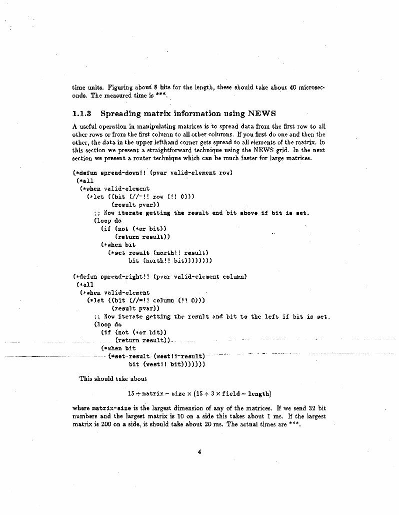
time units. Figuring about 8 bits for the length, these should take about 40 microsec· onds. The measured time is ***. .

1.1.3 Spreading matrix information using NEWS

A useful operation in manipulating matrices is to spread data from the first row to all other rows or from the first column to all other columns. If you first do one and then the other, the data in the upper lefthand corner gets spread to all elements of the matrix. In this section we present a straightforward technique using the NEWS grid. In the next section we present a router technique which can be much faster for large matrices.

(*defun spread-down!! (pvar valid-element row) (*all .

(*when valid-element (*let «bit (II-!! row (!! 0»)

(result pvar» :; Now iterate getting the result and bit above if bit is set. (loop do

(if (not (*or bit» (return result»

(*when bit (*set result (north!! result)

bit (north!! bit»»»»

(*defun spread-right!! (pvar valid-element column) (*all

(*when valid-element (.let «bit (II-!! column (!! 0»)

(result pvar» ;; Now iterate getting the result and bit to the left if bit is set. (loop do

(if (not (*or bit» (return result) ) ..

(*when bit - (*set- result~ (west!i-result) -.~~.. -.-.

bit (west!! bit»»»)

This should take about

15 + matrix - size X (15 + 3 X field - length)

where matrix-size is the largest dimension of any of the matrices. If we send 32 bit numbers and the largest matrix is 10 on a side this takes about 1 ms. If the largest matrix is 200 on a side, it should take about 20 ms. The actual times are .....

4

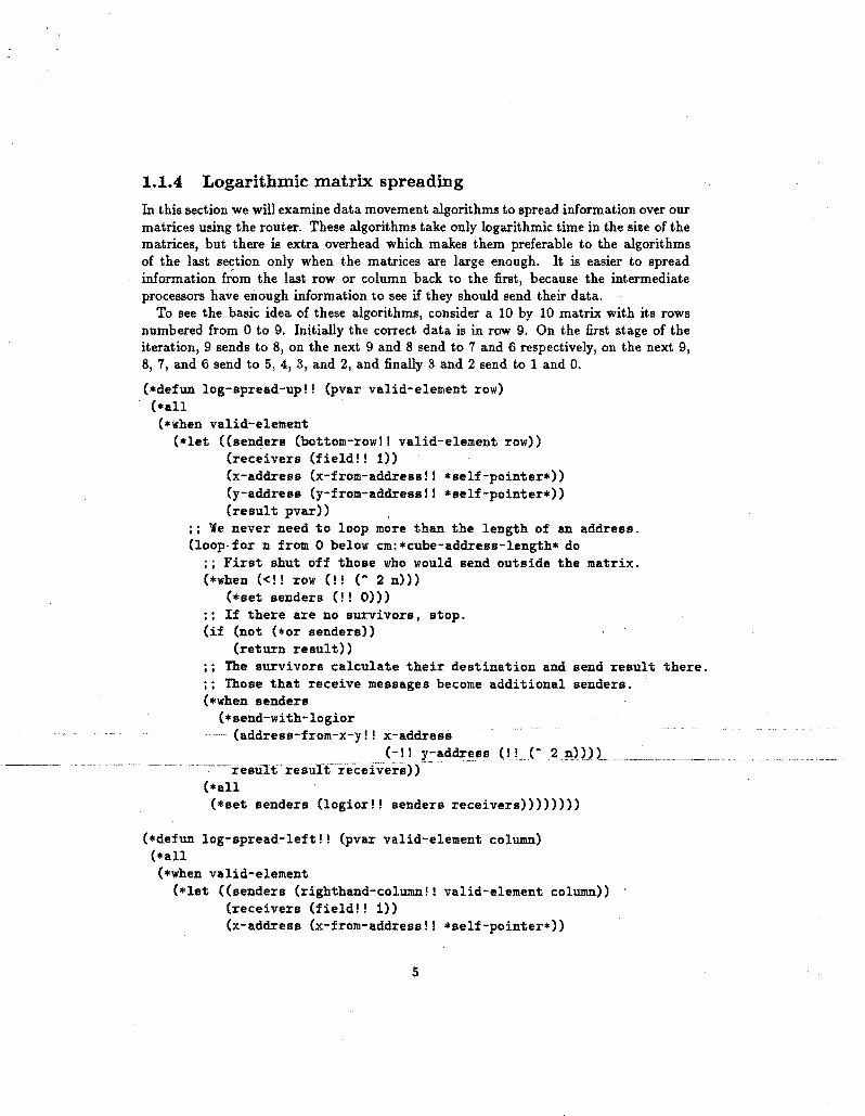
1.1.4 Logarithmic matrix sprea.ding

In this section we will examine data movement algorithms to spread information over our matrices using the router. These algorithms take only logarithmic time in the size of the matrices, but there is extra overhead which makes them preferable to the algorithms of the last section only when the matrices are large enough. It is easier to spread information fiom the last row or column back to the first, because the intermediate processors have enough information to see if they should send their data.

To see the basic idea of these algorithms, consider a 10 by 10 matrix with its rows numbered from 0 to 9. Initially the correct data is in row 9. On the first stage of the iteration, 9 sends to 8, on the next 9 and 8 send to 7 and 6 respectively, on the next 9, 8, 7, and 6 send to 5, 4, 3, and 2, and finally 3 and 2 send to 1 and O.

(*defun log-spread-up!! (pvar valid-element row) (*all (*when valid-element

(*let «senders (bottom-row!! valid-element row» (receivers (field!! 1» (x-address (x-from-address!! *self-pointer*» (y-address (y-from-address!! *self-pointer*» (result pvar»

" We never need to loop more than the length of an address. (loop-for n from 0 below cm:*cube-address-length* do

;; First shut off those who would send outside the matrix. (*when «!! row (I! (~ 2 n»)

(*set senders (!! 0») ;; If there are no survivors, stop. (if (not (*or senders»

(return result» ;; The survivors calculate their destination and send result there. ;; Those that receive messages become additional senders. (*when senders

(*send-with-logior (address-from-x-yl! x-address

(-I! y-address (!L(~2J.1)U

···-----resu-rt·iesu1t~receivers) f ­(*all (*set senders (logior!! senders receivers»»»»

(*defun log-spread-left!! (pvar valid-element column) (*all (*when valid-element

(*let «senders (righthand-column!! valid-element column» (receivers (field!! 1» (x-address (x-from-address!! *self-pointer*»

5

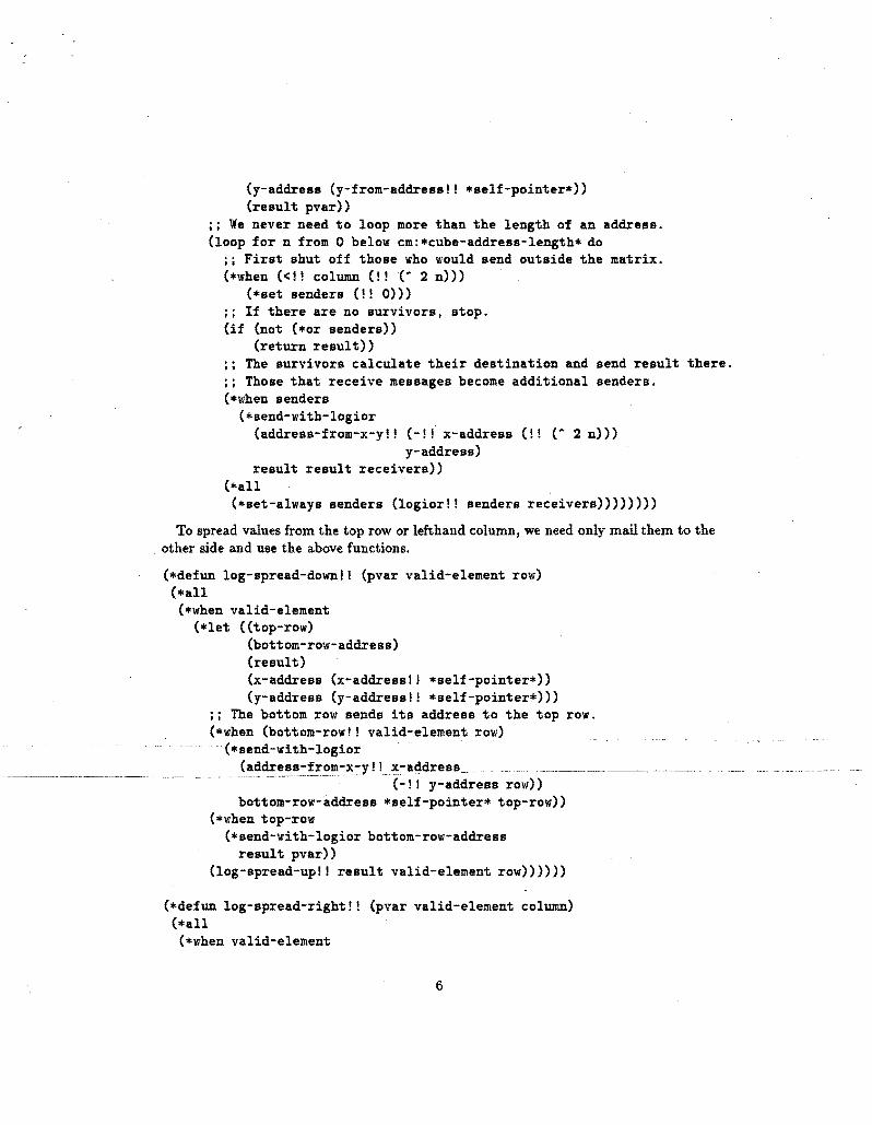
(y-address (y-from-address!! *self-pointer*» (result pvar»

" We never need to loop more than the length of an address. (loop for n from 0 below cm:*cube-address-length* do

;; First shut off those who would send outside the matrix. (*when «!! column (I! (- 2 n»)

(*set senders (!! 0») ;; If there are no survivors. stop. (if (not (*or senders»

(return result» ;; The survivors calculate their destination and send result there. ;; Those that receive messages become additional senders. (*when senders

(*send-with-logior (address-from-x-y!! (-!! x-address (!! (- 2 n»)

y-address) result result receivers»

(*a11 (*set-always senders (logior!! senders receivers»»»»

To spread values from the top row or lefthand column, we need only mail them to the other side and use the above functions.

(*defun log-spread-downl! (pvar valid-element row) (*a11

(*when valid-element (*let «top-row)

(bottom-row-address) (result) (x-address (x-addressl! *self-pointer*» (y-address (y-address!! *self-pointer*»)

•• The bottom row sends its address to the top row. (*when (bottom-row!! valid-element row)

(*send-with-logior­(address-from-x-y! !~~::alidress___ _ ________ ~_..

----------..... (-!! y-address row»

bottom-row-address "'self-pointer* top-row» (*when top-row

(*send-with-logior bottom-row-address result pvar»

(log-spread-up!! result valid-element row»»»

(*defun log-spread-right!! (pvar valid-element column) (*a11

(*when valid-element

6

(*let «left-column) (right-column-address) (result) (x-address (x-address! 1 *self-pointer*» (y-address (y-address!1 *self-pointer*»)

•• The righthand column sends its address to the lefthand one. (*when (righthand-columnl 1 valid-element column)

(*send-with-logior (address-from-x-y!! (-I! x-address column)

y-address) right-column-address *self-pointer* left-column»

(*select left-column (*send-with-logior right-column-address

result pvar» (log-spread-left!! result valid-element column»»»

Let us compare the timings for this type of spreading with the pure NEWS spreading.

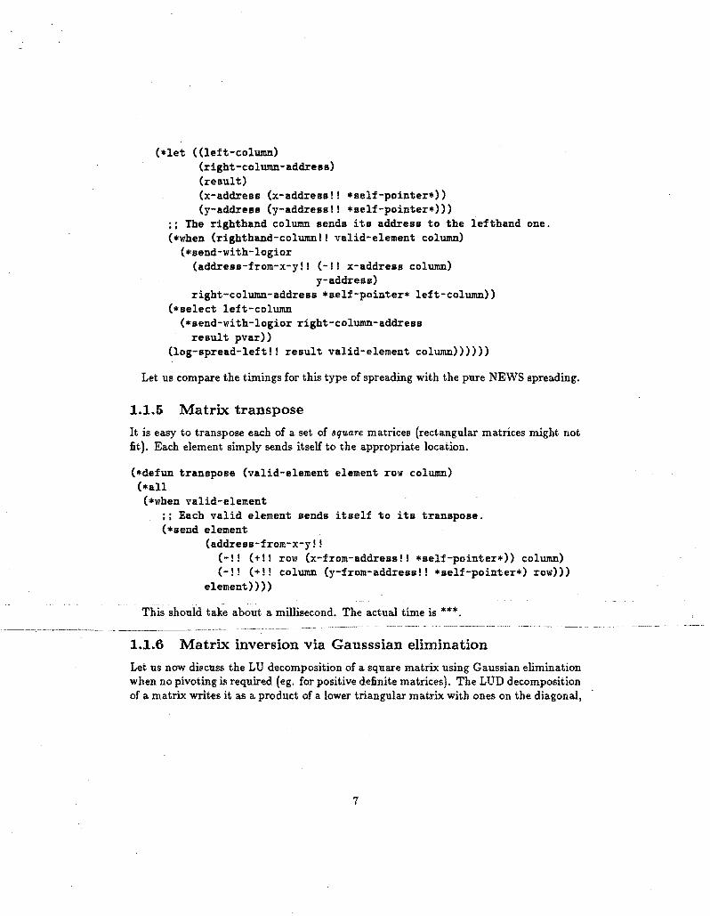
1.1.5 Matrix transpose

It is easy to transpose each of a set of square matrices (rectangular matrices might not fit). Each element simply sends itself to the appropriate location.

(*defun transpose (valid-element element row column) (*all (*when valid-element

;; Each valid element sends itself to its transpose. (*send element

(address-from-x-yll (-!I (+11 row (x-from-address!! *self-pointer*» column) (-I! (+I! column (y-from-addressl! *self-pointer*) row»)

element» » < «

This should tak~ about a millisecond. The actual time is ***.

1.1.6 Matrix inversion via Gausssian elimination

Let us now discuss the LU decomposition of a square matrix using Gaussian elimination when no pivoting is required (eg. for positive definite matrices). The LUD decomposition of a matrix writes it as a product of a lower triangular matrix with ones on the diagonal,

7

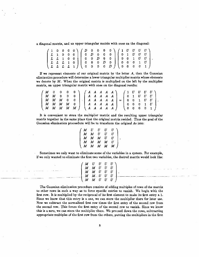
a diagonal matrix, and an upper triangular matrix with ones on the diagonal:

0 0 0 0 0 U U0][ D1 0 oo 0 0 D 0 0 oo ][ 01 U1 U U L 1 o 0 0 0 D 0 o 0 0 1 U L L 1 0 0 0 0 D o 0 0 0 1 L L L 1 0 0 0 0 D 0 0 0 0U n·

H we represent elements of our original matrix by the letter A, then the Gaussian elimination procedure will determine a lower triangular multiplier matrix whose elements we denote by M. When the original matrix is multiplied on the left by the multiplier matrix, an upper triangular matrix with ones on the diagonal results:

[ ~~l ~ ~].[~~ ~~~]=[~r ~gg].MMMM 0 AAAAA 0001 U MMMMM AAAAA 00001

It is convenient to store the multiplier matrix and the resulting upper triangular matrix together in the same place that the original matrix resided. Thus the goal of the Gaussian elimination proceedure will be to transform the original As into:

MUUUU]M M U U U M M M U U .

[ M M M M U M M M M M

Sometimes we only want to eliminate some of the variables in a system. For example, if we only wanted to eliminate the first two variables, the desired matrix would look like:

The Gaussian elimination procedure consists of adding multiples of rows of the matrix to other rows in such a way as to force specific entries to vanish. We begin with the first row. It is multiplied by the reciprocal of its first element to make its first entry a 1. Since we know that this entry is a one, we can store the multiplier there for later use. Now we subtract the normalized first row times the first entry of the second row from the second row. This forces the first entry of the second row to vanish. Since we know this is a zero, we can store the multiplier there. We proceed down the rows, subtracting appropriate multiples of the first row from the others, putting the multipliers in the first

8

column. Now we continue with the second row, eliminating entries in the second column below it. Again the multipliers are placed in the second column. This continues until all the desired variables are eliminated.

We will implement a very nice systolic algorithm to do this elimination. The active elements proceed in a diagonal wave from the upper left hand corner of the matrix to the lower right. Because the multiplications are the most time consuming part of the algorithm, we organize things so that as many multiplies occur simultaneously as possible.

In this algorithm data moves from left to right and from top to bottom. To describe the computations involved, we will utilize three fields in the connection machine, each capable of holding a matrix entry. Mwill hold the original matrix and the final result. R will hold rightward moving data and will be shifted to the right on each iteration step. D will hold downward moving data and will be shifted down on each iteration step. There are four classes of operations that can be performed at a given matrix location and at most one will be performed at a given location on a given iteration step. Let us label them A, B, C, and D:

A These occur only on the diagonal. They find the reciprocal of the element in M and put it into R, D, and M.

B These occur along a row that is to be eliminated. They multiply by the reciprocal of the first element of the row and start the value in that column of the row moving downward to be subtracted from other rows. The operation is to take the product of M and R and put the result into M and D.

C These occur along the first column of a row to be eliminated. They start the value of a multiplier moving to the right along a row. The operation is to first put Minto R and then to take the product of M and D and put minus the result into M.

D These actually cause the elimination and occur anywhere one row is being subtracted from another one. The operation is to put M minus R times D into M.

Let us now see where these operations occur in the matrix after various time steps. We will put an A.. B, C, or Din the matrix locations whose processor's are doing the corresponding operation and '" in those which do nothing. The first step is to do and A

____.._.__.. ~..~__.....~.._.___- the upper. lefthand-corner:-·· .

~::::l( '" '" '" '" '" . '" '" '" '" '" '" '" '" '" ..

Now field R is shifted one to the right, field D is shifted one down and we have the information to do a B in the second element of the first row and a C in the second

9

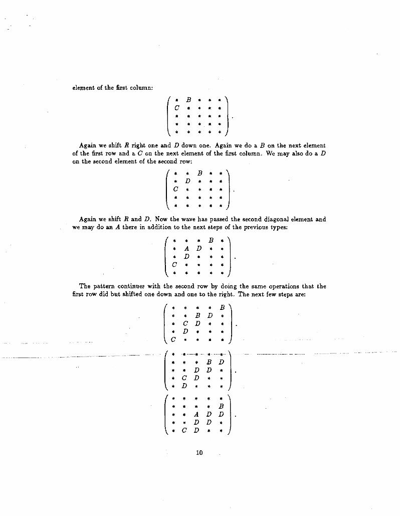
element of the first column:

Again we shift R right one and D down one. Again we do a B on the next element of the first row and a 0 on the next element of the first column. We may also do a D on the second element of the second row:

Again we shift Rand D. Now the wave has passed the second diagonal element and we may do an A there in addition to the next steps of the previous types:

'" '" '" B '" AD",

'" D '" '" [ o '" '" '"

'" '" '" '" The pattern continues with the second row by doing the same operations that the

first row did but shifted one down and one to the right. The next few steps are:

10

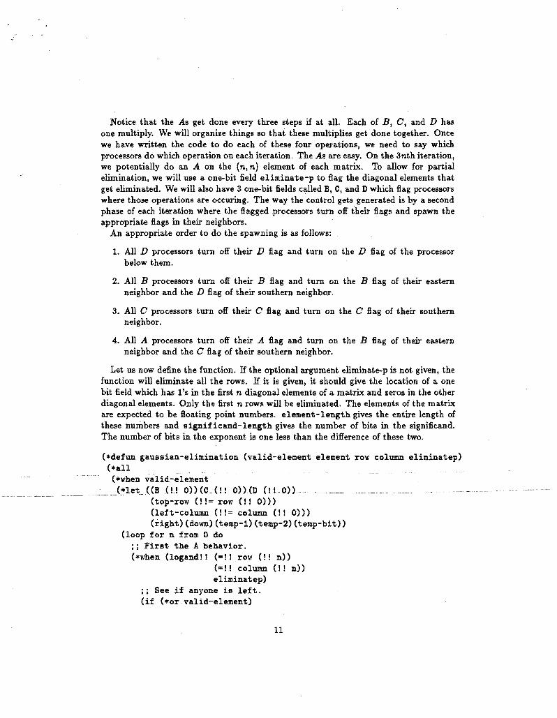
Notice that the As get done every three steps if at all. Each of B, 0, and D has one multiply. We will organize things so that these multiplies get done together. Once we have written the code to do each of these four operations, we need to say which processors do which operation on each iteration. The As are easy. On the 3nth iteration, we potentially do an A on the (n, n) element of each matrix. To allow for partial elimination, we will use a one-bit field eliminate-p to flag the diagonal elements that get eliminated. We will also have 3 one-bit fields called B, C, and D which flag processors where those operations are occuring. The way the control gets generated is by a second phase of each iteration where the flagged processors turn off their flags and spawn the appropriate flags in their neighbors.

An appropriate order to do the spawning is as follows:

1. All D processors turn off their D flag and turn on the D flag of the processor below them.

2. All B processors turn off their B flag and turn on the B flag of their eastern neighbor and the D flag of their southern neighbor.

3. All 0 processors turn off their 0 flag and turn on the 0 flag of their southern neighbor.

4. All A processors turn off their A flag and turn on the B flag of their eastern neighbor and the 0 flag of their southern neighbor.

Let us now define the function. If the optional argument eliminate-p is not given, the function will eliminate all the rows. If it is given, it should give the location of a one bit field which has l's in the first n diagonal elements of a matrix and zeros in the other diagonal elements. Only the first n rows will be eliminated. The elements of the matrix are expected to be floating point numbers. element-length gives the entire length of these numbers and significand-length gives the number of bits in the significand. The number of bits in the exponent is One less than the difference of these two.

(*defun gaussian-elimination (valid-element element row column eliminatep) (*all

(*when valid-element J....let_f(B eU O»(C.(.LLD»(D (1LO»

.._-_._--­(top-row (!!= row (!! 0») (left-column (!I= column (!I 0») (right) (down) (temp-1) (temp-2) (temp-bit»

(loop for n from 0 do ;; First the A behavior .. (*when (logand!! ( .. !! row (! In»

(=I! column (II n» eliminatep)

;; See if anyone is left. (if (*or valid-element)

11

(progn ;; Load up right, down, and element with reciprocal of element. (*set right (II!! (!l 1) element)

down right element right» i; No A's left, if no D's then quit. (if (not (*or D»

(return») :: Now the B, C, D behavior for three iterations. (dotimes (i 3)

(*when C (*set right element temp-1 down» (*when (logior!! B C) (*set temp-2 element» (*when D (*set temp-2 down» (*when (logior!! B D) (*set temp-1 right» :; Do all the multiplies in one shot. (*when (logior!! BCD) (*set temp-1 (*11 temp-1 temp-2») (*when B (*set down temp-1» (*when (logior!! B C) (*set element temp-1» (*when D (*set element (-!! element temp-1») ;; Now we update the B, C, and D fields. (*set D (north'! D» (*when top-row (*set D (I! 0») (*set temp-bit (north!! B» (*when top-row (*set temp-bit (!! 0») (*set D (logior!! D temp-bit» (*set B (west!! B» (*when left-column (*set B (!! 0») i; Next C moves down one, putting 0 in the top row. (*set C (north!! e» (*when top-row (*set C (I! 0») ;; Only do the A updates if we are on the first iteration. (if (= i 0) .

(progn ;; First set the B's. (*when (logand" (==!! row (!! n»

-~-- -C";'!! column(! ,- (1+ n»» (*set B O! 1»)

(*when (logand!! (=I! row (!! (1+ n») (=!! column (!! n»)

(*sete (I! 1»»»

12