numerical optimization: basic concepts and algorithms · r.duvigneau-numericaloptimization:...
TRANSCRIPT
R. Duvigneau - Numerical Optimization: Basic Concepts and Algorithms 1
May 27th 2015
Numerical Optimization:Basic Concepts and AlgorithmsR. Duvigneau
Outline
I Some basic concepts in optimizationI Some classical descent algorithmsI Some (less classical) semi-deterministic approachesI Illustrations on various analytical problemsI Constrained optimalityI Some algorithm to account for constraints
R. Duvigneau - Numerical Optimization: Basic Concepts and Algorithms 2

R. Duvigneau - Numerical Optimization: Basic Concepts and Algorithms 3
Some basic concepts
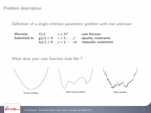
Problem description
Definition of a single-criterion parametric problem with real unknown
Minimize f (x) x ∈ Rn cost fonctionSubmitted to gi (x) = 0 i = 1, · · · , l equality constraints
hj (x) > 0 j = 1, · · · ,m inequality constraints
What does your cost function look like ?
Convex problem Multi-modal problem Noisy problem
R. Duvigneau - Numerical Optimization: Basic Concepts and Algorithms 4
Some commonly used algorithms
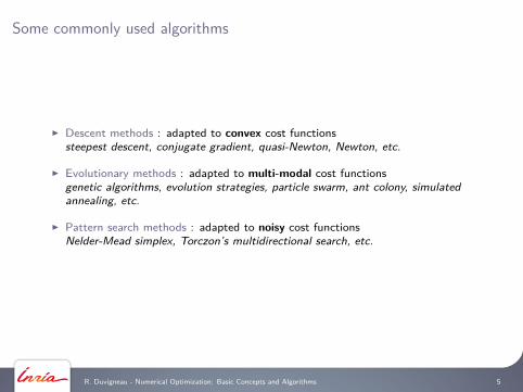
I Descent methods : adapted to convex cost functionssteepest descent, conjugate gradient, quasi-Newton, Newton, etc.
I Evolutionary methods : adapted to multi-modal cost functionsgenetic algorithms, evolution strategies, particle swarm, ant colony, simulatedannealing, etc.
I Pattern search methods : adapted to noisy cost functionsNelder-Mead simplex, Torczon’s multidirectional search, etc.
R. Duvigneau - Numerical Optimization: Basic Concepts and Algorithms 5
Optimality conditions
Definition of a minimum
x? is a minimum of f : Rn 7→ R if and only if there exists ρ > 0 such as:I f defined on B(x?, ρ)
I f (x?) < f (y) ∀y ∈ B(x?, ρ) y 6= x?
→ not very useful to build algorithms ...
Characterization
A sufficient condition for x? to be a minimum is (if f twice differentiable):I ∇f (x?) = 0 (stationarity of gradient vector)I ∇2f (x?) > 0 (Hessian matrix positive definite)
R. Duvigneau - Numerical Optimization: Basic Concepts and Algorithms 6
R. Duvigneau - Numerical Optimization: Basic Concepts and Algorithms 7
Some classical descent algorithms
Descent methods
Model algorithm
For each iteration k (starting from xk):
I Evaluate gradient ∇f (xk )
I Define a search direction dk (∇f (xk ))
I Line search : choice of step length ρk
I Update: xk+1 = xk + ρkdk
R. Duvigneau - Numerical Optimization: Basic Concepts and Algorithms 8
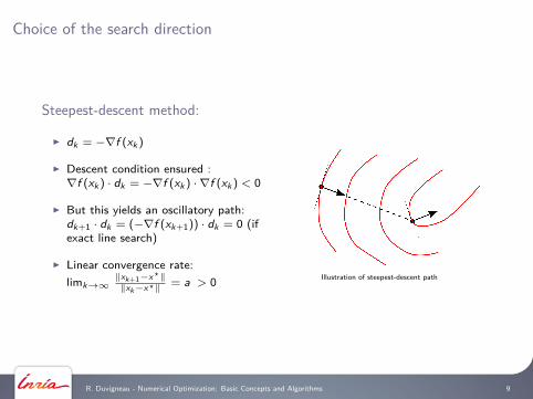
Choice of the search direction
Steepest-descent method:
I dk = −∇f (xk )
I Descent condition ensured :∇f (xk ) · dk = −∇f (xk ) · ∇f (xk ) < 0
I But this yields an oscillatory path:dk+1 · dk = (−∇f (xk+1)) · dk = 0 (ifexact line search)
I Linear convergence rate:limk→∞
‖xk+1−x?‖‖xk−x?‖ = a > 0 Illustration of steepest-descent path
R. Duvigneau - Numerical Optimization: Basic Concepts and Algorithms 9
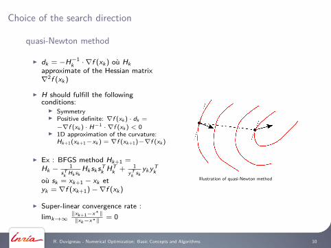
Choice of the search direction
quasi-Newton method
I dk = −H−1k · ∇f (xk ) où Hkapproximate of the Hessian matrix∇2f (xk )
I H should fulfill the followingconditions:
I SymmetryI Positive definite: ∇f (xk ) · dk =
−∇f (xk ) · H−1 · ∇f (xk ) < 0I 1D approximation of the curvature:
Hk+1(xk+1−xk ) = ∇f (xk+1)−∇f (xk )
I Ex : BFGS method Hk+1 =Hk − 1
sTk Hk sk
HksksTk HT
k + 1yT
k skykyT
k
où sk = xk+1 − xk etyk = ∇f (xk+1)−∇f (xk )
I Super-linear convergence rate :limk→∞
‖xk+1−x?‖‖xk−x?‖ = 0
Illustration of quasi-Newton method
R. Duvigneau - Numerical Optimization: Basic Concepts and Algorithms 10
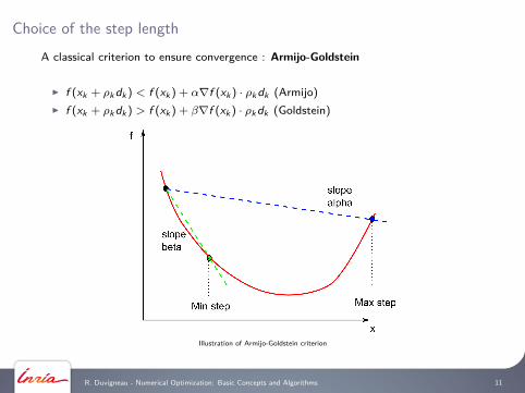
Choice of the step lengthA classical criterion to ensure convergence : Armijo-Goldstein
I f (xk + ρkdk ) < f (xk ) + α∇f (xk ) · ρkdk (Armijo)I f (xk + ρkdk ) > f (xk ) + β∇f (xk ) · ρkdk (Goldstein)
Illustration of Armijo-Goldstein criterion
R. Duvigneau - Numerical Optimization: Basic Concepts and Algorithms 11
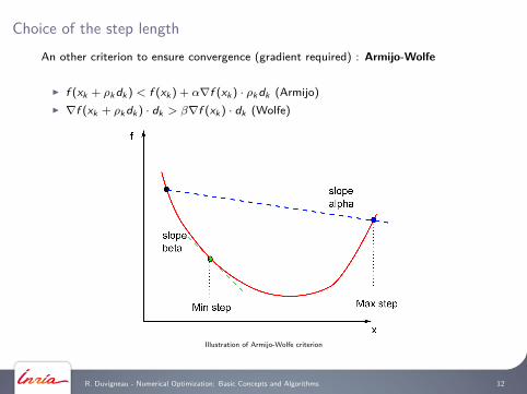
Choice of the step lengthAn other criterion to ensure convergence (gradient required) : Armijo-Wolfe
I f (xk + ρkdk ) < f (xk ) + α∇f (xk ) · ρkdk (Armijo)I ∇f (xk + ρkdk ) · dk > β∇f (xk ) · dk (Wolfe)
Illustration of Armijo-Wolfe criterion
R. Duvigneau - Numerical Optimization: Basic Concepts and Algorithms 12
Choice of the step length
The step length is determined using an iterative 1D search:
I Start from an initial guess ρ(p)k (p = 0)
I Update to ρ(p+1)k :
I Bisection methodI Polynomial interpolationI ...
I until stopping criteria are fulfilled
A balance is necessary between the computational cost and the accuracy
R. Duvigneau - Numerical Optimization: Basic Concepts and Algorithms 13
R. Duvigneau - Numerical Optimization: Basic Concepts and Algorithms 14
Some (less classical) semi-deterministic approaches
Evolutionary algorithms
Principles
Inspired by Darwinian theory of evolution :
I A population is composed of individuals who have different characteristics
I Most fitted individuals can survive and reproduce
I An offspring population is generated from survivors
→ Mechanisms to improve progressively the population performance !
R. Duvigneau - Numerical Optimization: Basic Concepts and Algorithms 15
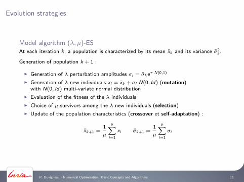
Evolution strategies
Model algorithm (λ, µ)-ESAt each iteration k, a population is characterized by its mean x̄k and its variance σ̄2k .
Generation of population k + 1 :
I Generation of λ perturbation amplitudes σi = σ̄keτ N(0,1)
I Generation of λ new individuals xi = x̄k + σi N(0, Id) (mutation)with N(0, Id) multi-variate normal distribution
I Evaluation of the fitness of the λ individualsI Choice of µ survivors among the λ new individuals (selection)I Update of the population characteristics (crossover et self-adaptation) :
x̄k+1 =1µ
µ∑i=1
xi σ̄k+1 =1µ
µ∑i=1
σi
R. Duvigneau - Numerical Optimization: Basic Concepts and Algorithms 16
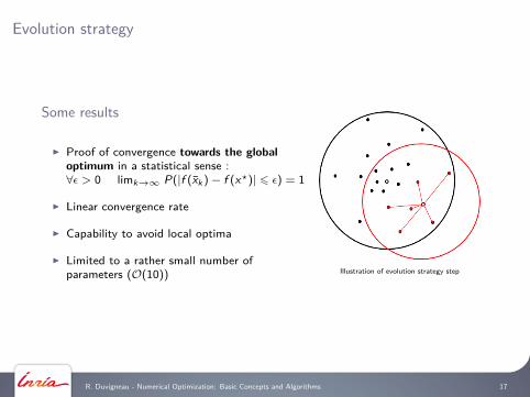
Evolution strategy
Some results
I Proof of convergence towards the globaloptimum in a statistical sense :∀ε > 0 limk→∞ P(|f (x̄k )− f (x?)| 6 ε) = 1
I Linear convergence rate
I Capability to avoid local optima
I Limited to a rather small number ofparameters (O(10)) Illustration of evolution strategy step
R. Duvigneau - Numerical Optimization: Basic Concepts and Algorithms 17
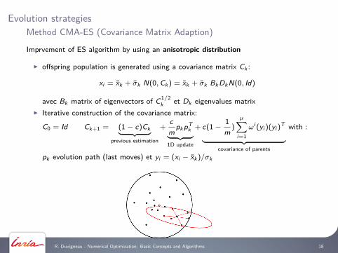
Evolution strategiesMethod CMA-ES (Covariance Matrix Adaption)
Imprvement of ES algorithm by using an anisotropic distribution
I offspring population is generated using a covariance matrix Ck :
xi = x̄k + σ̄k N(0,Ck ) = x̄k + σ̄k BkDkN(0, Id)
avec Bk matrix of eigenvectors of C1/2k et Dk eigenvalues matrix
I Iterative construction of the covariance matrix:
C0 = Id Ck+1 = (1− c)Ck︸ ︷︷ ︸previous estimation
+cm
pkpTk︸ ︷︷ ︸
1D update
+ c(1−1m
)
µ∑i=1
ωi (yi )(yi )T
︸ ︷︷ ︸covariance of parents
with :
pk evolution path (last moves) et yi = (xi − x̄k )/σk
R. Duvigneau - Numerical Optimization: Basic Concepts and Algorithms 18
R. Duvigneau - Numerical Optimization: Basic Concepts and Algorithms 19
Some illustrations using analytical functions
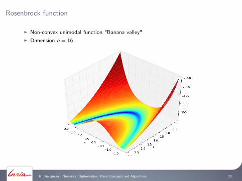
Rosenbrock function
I Non-convex unimodal function "Banana valley"I Dimension n = 16
R. Duvigneau - Numerical Optimization: Basic Concepts and Algorithms 20
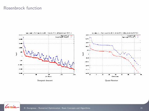
Rosenbrock function
Steepest descent Quasi-Newton
R. Duvigneau - Numerical Optimization: Basic Concepts and Algorithms 21
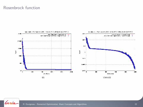
Rosenbrock function
ES CMA-ES
R. Duvigneau - Numerical Optimization: Basic Concepts and Algorithms 22
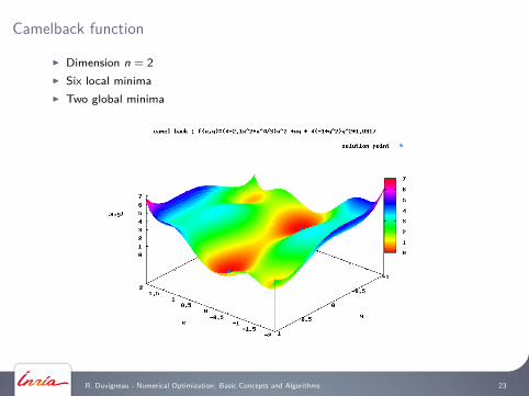
Camelback function
I Dimension n = 2I Six local minimaI Two global minima
R. Duvigneau - Numerical Optimization: Basic Concepts and Algorithms 23
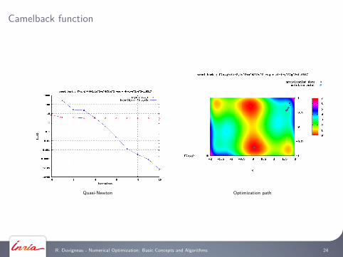
Camelback function
Quasi-Newton Optimization path
R. Duvigneau - Numerical Optimization: Basic Concepts and Algorithms 24
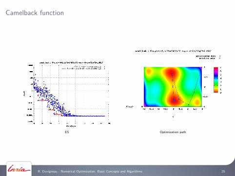
Camelback function
ES Optimization path
R. Duvigneau - Numerical Optimization: Basic Concepts and Algorithms 25

R. Duvigneau - Numerical Optimization: Basic Concepts and Algorithms 26
Constrained optimality
Introduction
Necessity of constraintsI Often required to define a well-posed problem from mathematical point of view
(existence, unicity)
I Often required to define a problem that make sense from industrial point ofview (manufacturing)
Different types of constraintsI Equality / inequality constraints
I Linear / non-linear constraints
R. Duvigneau - Numerical Optimization: Basic Concepts and Algorithms 27

Linear contraints
Optimality conditions
A sufficient condition for x? to be a minimum of f subject to A · x = b :I A · x? = b (admissibility)I ∇f (x?) = λ? · A with λ? Lagrange multipliers (stationnarity)I A · ∇2f (x?) · A > 0 (projected Hessian positive definite)
Illustration of optimality conditions for linear constraints
R. Duvigneau - Numerical Optimization: Basic Concepts and Algorithms 28
Linear constraints
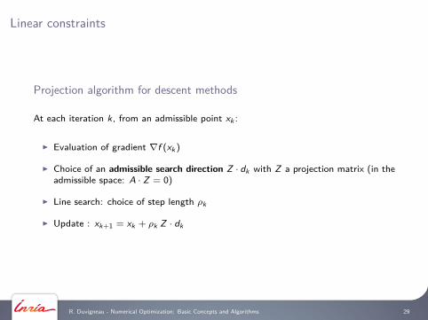
Projection algorithm for descent methods
At each iteration k, from an admissible point xk :
I Evaluation of gradient ∇f (xk )
I Choice of an admissible search direction Z · dk with Z a projection matrix (in theadmissible space: A · Z = 0)
I Line search: choice of step length ρk
I Update : xk+1 = xk + ρk Z · dk
R. Duvigneau - Numerical Optimization: Basic Concepts and Algorithms 29
Non-linear constraints
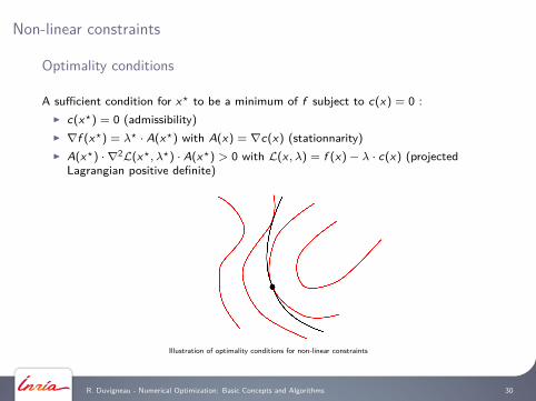
Optimality conditions
A sufficient condition for x? to be a minimum of f subject to c(x) = 0 :I c(x?) = 0 (admissibility)I ∇f (x?) = λ? · A(x?) with A(x) = ∇c(x) (stationnarity)I A(x?) · ∇2L(x?, λ?) · A(x?) > 0 with L(x , λ) = f (x)− λ · c(x) (projected
Lagrangian positive definite)
Illustration of optimality conditions for non-linear constraints
R. Duvigneau - Numerical Optimization: Basic Concepts and Algorithms 30
Non-linear constraints
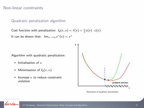
Quadratic penalization algorithm
Cost function with penalization: fq(x , κ) = f (x) + κ2 c(x) · c(x)
It can be shown that: limκ→∞x?(κ) = x?
Algorithm with quadratic penalization:
I Initialisation of κ
I Minimisation of fq(x , κ)
I Increase κ to reduce constraintviolation
Illustration of quadratic penalization
R. Duvigneau - Numerical Optimization: Basic Concepts and Algorithms 31
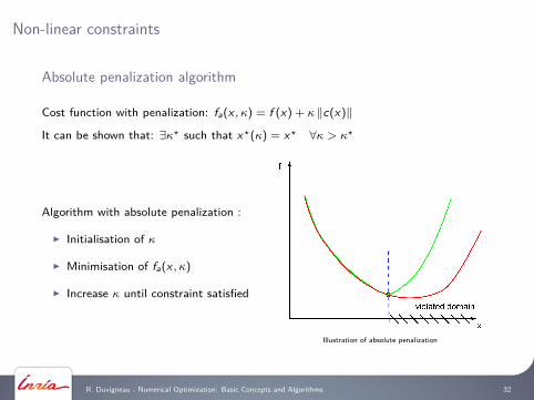
Non-linear constraints
Absolute penalization algorithm
Cost function with penalization: fa(x , κ) = f (x) + κ ‖c(x)‖
It can be shown that: ∃κ? such that x?(κ) = x? ∀κ > κ?
Algorithm with absolute penalization :
I Initialisation of κ
I Minimisation of fa(x , κ)
I Increase κ until constraint satisfied
Illustration of absolute penalization
R. Duvigneau - Numerical Optimization: Basic Concepts and Algorithms 32
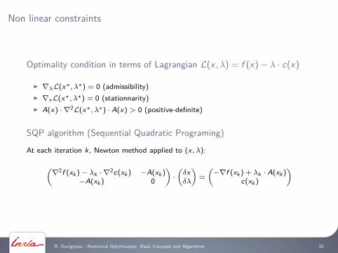
Non linear constraints
Optimality condition in terms of Lagrangian L(x , λ) = f (x)− λ · c(x)
I ∇λL(x?, λ?) = 0 (admissibility)I ∇xL(x?, λ?) = 0 (stationnarity)I A(x) · ∇2L(x?, λ?) · A(x) > 0 (positive-definite)
SQP algorithm (Sequential Quadratic Programing)
At each iteration k, Newton method applied to (x , λ):
(∇2f (xk )− λk · ∇2c(xk ) −A(xk )
−A(xk ) 0
)·(δxδλ
)=
(−∇f (xk ) + λk · A(xk )
c(xk )
)
R. Duvigneau - Numerical Optimization: Basic Concepts and Algorithms 33
Some references
Classical methods
I G. N. Venderplaats. Numerical optimization techniques for engineering design.McGraw-Hill, 1984.
I R. Fletcher. Practical Methods of Optimization. John Wiley & Sons, 1987.I P. E. Gill, W. Murray, and M. H. Wright. Practical Optimization. Academic
Press, 1981.
Evolutionary methodsI Z. Michalewics. Genetic algorithms + data structures = evolutionary programs.
AI series. Springer-Verlag, New York, 1992.I D. Goldberg. Genetic Algorithms in Search, Optimization and Machine Learning.
Addison Wesley Company Inc., 1989.
R. Duvigneau - Numerical Optimization: Basic Concepts and Algorithms 34