notes on consumer theory - university of manchester · title: notes on consumer theory author:...

Notes on Consumer Theory

Alejandro Saporiti

Alejandro Saporiti (Copyright) Consumer Theory 1 / 65

Consumer theory

Reference:Jehle and Reny,Advanced Microeconomic Theory, 3rd ed.,Pearson 2011: Ch. 1.

The economic model of consumer choice has 4 ingredients:

1. The consumption set;

2. The preference relation;

3. The feasible (budget) set;

4. Behavioral assumptions (e.g., rationality).

This basic structure gives rise to a generaltheory of choicewhich is used inseveral social sciences (e.g., economics & political science).

For concreteness, we focus on explaining the behavior (choices) of arepresentative consumer, a central actor in much of economic theory.


Consumption set

The consumption or choice set represents the set of all alternatives availableto the (unrestricted) consumer.

In economics, these alternatives are calledconsumption plans.

A consumption plan represents a bundle of goods, and is written as a vectorxconsisting ofn different consumption goods,x = (x1, . . . , xn).

Typical assumptions onX are:

1. ∅ 6= X ⊆ Rn+ (i.e., nonempty & each good measured in infinitely

divisible and nonnegative units);

2. X is closed;

3. X is convex;

4. 0 ∈ X.


Consumer preferences

Consumer’s preferences represent his attitudes toward theobjects of choice.

The consumer is born with these attitudes, i.e. preferencesare a ‘primitive’ inclassical consumer theory.

To represent them formally, we use theat least as good asbinary relation% onX; and for any two bundlesx1 andx2, we say that,

1. The consumer isindifferentbetweenx1 andx2, denoted byx1 ∼ x2, ifand only if (iff) x1 % x2 andx2 % x1;

2. The consumerstrictly prefersx1 overx2, indicated byx1 ≻ x2, iffx1 % x2 and¬[x2 % x1].


Consumer preferencesWe require% to satisfy the following axioms:

1. Completeness: For all x1 andx2 in X, eitherx1 % x2 or x2 % x1;

2. Transitivity: For any three bundlesx1, x2 andx3 in X, if x1 % x2 andx2 % x3, thenx1 % x3.

When% satisfies these axioms it is said to be arational preference relation.

Under completeness and transitivity, for any two bundlesx1, x2 ∈ X, exactlyone of the following three possibilities holds: either

◮ x1 ≻ x2,◮ x2 ≻ x1, or◮ x1 ∼ x2.

Thus, the rational preference relation% offers aweak or partial orderof X(complete and transitive), ranking any finite number of alternatives inX frombest to worst, possibly with some ties.


Consumer preferencesApart from Axioms 1 & 2, we demand three additional properties on%:

3. Continuity: For all x0 ∈ X, the sets{x ∈ X : x % x0} and{x ∈ X : x0 % x} are closed inX ⊂ R

n+;

◮ Continuity rules out openareas in the indifference set;that is, the set{x ∈ X : x ∼ x0} = {x ∈ X :x % x0} ∩ {x ∈ X : x0 % x} isclosed.

◮ It rules out ‘suddenpreference reversals’ such asthe one happening in Fig 1,where(b, 0) ≻ℓ (x, 1) for allx < b, but(b, 1) ≻ℓ (b, 0).

Figure 1:Lexicographic preferences%ℓ

onR2+; (a1, a2) %ℓ (b1, b2) iff either

a1 > b1, or a1 = b1 anda2 ≥ b2.



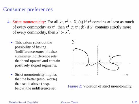
4. Strict monotonicity: For all x1, x2 ∈ X, (a) if x1 contains at least as muchof every commodity asx2, thenx1 % x2; (b) if x1 contains strictly moreof every commodity, thenx1 ≻ x2.

◮ This axiom rules out thepossibility of having‘indifference zones’; it alsoeliminates indifference setsthat bend upward and containpositively sloped segments.

◮ Strict monotonicity impliesthat the better (resp. worse)than set is above (resp.below) the indifference set. Figure 2:Violation of strict monotonicity.



5. Strict convexity: For all x1, x2 ∈ X, if x1 6= x2 andx1 % x2, then for allα ∈ (0, 1), αx1 + (1− α)x2 ≻ x2.

◮ It rules out concave to the origin segments in the indifference sets.◮ It prevents the consumer from preferring extremes in consumption.

x1

x2

x2

x1

αx1 + (1 − α)x2

Figure 3:Convex

x1

x2

x2

x1

α x1 + (1 − α)x2

Figure 4:Nonconvex


Consumer preferencesAxioms 3-5 exploit the structure of the spaceX:

◮ Continuity uses the ability to talk about closeness.

◮ Monotonicity uses the orderings on the axis (the ability to comparebundles by the amount of any particular commodity).

◮ It gives commodities the meaning of ‘goods’:More is better.

◮ Convexity uses the algebraic structure (the ability to speak of the sum oftwo bundles and the multiplication of a bundle by a scalar).

◮ That is, it assumes the existence a “geography” of the set of alternatives,so that we can talk about one alternative being between two others.

◮ It’s appropriate when the argument “if a move is an improvement so isany move part of the way” is legitimate, while the argument “if a move isharmful then so is a move part of the way” is not.


Utility representationWhen preferences are defined over large sets of alternatives, it is usuallyconvenient to employ calculus methods to work out the best options.

To do that, we’d like to represent the information conveyed by the preferencerelation% through a function.

A real-valued functionu : Rn+ → R is said to be autility representationof the

preference relation% if for all x1, x2 ∈ X ⊆ Rn+

x1 % x2 ⇔ u(x1) ≥ u(x2). (1)

Theorem 1 (Debreu, 1954)If the preference relation % is complete, transitive and continuous, then itpossesses a continuous utility representation u : R

n+ → R.

Consistent pair-wise comparability overX and some topological regularity areenough for a numerical representation of%.


Invariance of the utility functionTheordinal natureof the utility representation embedded in (1) implies that autility function u : R

n+ → R is unique up to any strictly increasing

transformation.

More formally, supposeu : Rn+ → R represents the preference relation%.

Then, for any strictly increasing transformationf : R → R, the function

v(x) ≡ f (u(x)) ∀x ∈ X, (2)

also represents%.

To see this, recall thatu(·) represents% if for all x, y ∈ X,

x ≻ y ⇔ u(x) > u(y), (3)

x ∼ y ⇔ u(x) = u(y). (4)


Invariance of the utility functionMoreover, note that for any two real numbersa, b ∈ R,

(i) f (a) > f (b) if and only if a > b; and

(ii) f (a) = f (b) if and only if a = b.

Thus, using the definition ofv given in (2) and (i)-(ii), for allx, y ∈ X

v(x) > v(y) ⇔ f (u(x)) > f (u(y)) ⇔ u(x) > u(y), (5)

v(x) = v(y) ⇔ f (u(x)) = f (u(y)) ⇔ u(x) = u(y). (6)

Combining (5) with (3), we have

v(x) > v(y) ⇔ x ≻ y.

Similarly, combining (6) with (4), we have

v(x) = v(y) ⇔ x ∼ y.

Hence,v(·) represents%.Alejandro Saporiti (Copyright) Consumer Theory 12 / 65

Quasiconcavity

A function u(·) is quasiconcaveon a convex setX ⊆ Rn if and only if for all

x, y ∈ X, and for allλ ∈ (0, 1),

u(λ x + (1− λ) y) ≥ min{u(x), u(y)}. (∗)

Strict quasiconcavity is defined analogously by replacing the weak inequalityin (∗) with the strict inequality.

A function g(·) is quasiconvexon a convex setX ⊆ Rn if and only if for all

x, y ∈ X, and for allλ ∈ (0, 1),

g(λ x + (1− λ) y) ≤ max{g(x), g(y)}.


Quasiconcavity

Alternatively, we could say that a functionu(·) is quasiconcaveon a convexsetX ⊆ R

n if for all c ∈ R the upper contour set{x ∈ X : u(x) ≥ c} is convex.


Quasiconcavity

xu(x)

u(x)

yy

Figure 5:Quasiconcave

xu(x)

u(x)

yy

Figure 6:Not quasiconcave

In the the picture above, every horizontal cut through the function must beconvex for the function to be quasi-concave. Thus,u(·) is quasiconcave inFig. 5, whereas it isn’t in Fig. 6.


Quasiconcavity

An important property of quasiconcavity is that it’s preserved underincreasing transformations.

Proposition 1If u : X ⊆ R

n → R is quasiconcave on X and φ : R → R is a monotoneincreasing transformation, then φ(u(·)) is quasiconcave.

The proof of Proposition 1 is as follows. We wish to show that for all x, y ∈ X,and for allλ ∈ (0, 1),

φ(u(λ x + (1− λ) y)) ≥ min{φ(u(x)), φ(u(y))}.


Quasiconcavity

Sinceu is quasiconcave, for allx, y ∈ X, and for allλ ∈ (0, 1),

u(λ x + (1− λ) y) ≥ min{u(x), u(y)}. (7)

Applying φ to both sides of (7),

φ(u(λ x + (1− λ) y)) ≥ φ(min{u(x), u(y)}). (8)

But,φ(min{u(x), u(y)}) = min{φ(u(x)), φ(u(y))}. (9)

Hence, combining (8) with (9), we get the desired result; that is, for allx, y ∈ X, and for allλ ∈ (0, 1),

φ(u(λ x + (1− λ) y)) ≥ min{φ(u(x)), φ(u(y))}.


Indifference curve & marginal utilityGiven a utility functionu(·), theindifference curve(level contour set) thatpasses through the bundlex ∈ X is defined as

{x ∈ X : u(x) = u(x)}.

If u(·) is quasiconcave, then the indifference curves are convex (recall Fig. 5:the upper contour sets of a quasi-concave function are convex).

If u is differentiable, then for alli = 1, . . . , n, themarginal utilityof xi

at x = (x1, . . . , xn) is

MUi(x) =∂u(x)∂xi

.

At x, consumer is willing tosubstitutex1 againstx2 at the rate of≈ −∆x1/∆x2. x1

x2

%

x

u(x)

∆x2

∆x1

−∆x1∆x2


Marginal rate of substitution

If we’d like to vary xi by a small amountdxi, while keeping utilityu(x)constant, how much do we need to changexj 6= xi?

Formally, the total differential ofu = u(x) is

0 =∂u(x)∂x1

dx1 + . . . +∂u(x)∂xn

dxn.

Since we only care about changes inxj caused by changes inxi, we setdxh = 0 for all h = 1, . . . , n, with h 6= i, j.

Thus, the total differential simplifies to

∂u(x)∂xi

dxi +∂u(x)∂xj

dxj = 0.


Marginal rate of substitutionRearranging the terms, we get that themarginal rate of substitution(MRS)between goodi and goodj is given by

MRSij(x) =dxj

dxi

∣∣∣du=0

= −∂u(x)/∂xi

∂u(x)/∂xj= −

MUi(x)MUj(x)

.

MRSij(x) is the rate at which goodj can be exchanged per unit of goodiwithout changing consumer’s utility.

◮ The absolute value of the MRSis equal to the ratio of marginalutilities of i andj at x;

◮ The MRS equals the slope of theindifference curve.

◮ When preferences are convex,the MRS between two goods isdecreasing.

u = u(x1, x2)

x1

x2 |MRS12(x0

1, x0

2)| > |MRS12(x1

1, x1

2)|

x01

x02

x12

x11


Budget set

Obviously, the consumer must be able to afford his consumption bundle. Thisgenerally restricts his choice set. We assume

◮ Each good has a strictly positive pricepi > 0, for all i = 1, . . . , n;

◮ The consumer is endowed with incomey > 0.

Thus consumer’s purchases are restricted by thebudget constraint

n∑

i=1

pixi ≤ y.

The budget set is the set of bundles that satisfy this constraint:

B(p, y) = {x ∈ X : p1x1 + . . . + pnxn ≤ y}.


Budget set (2-goods)

x1

x2

x1 = yp1

x2 = yp2

− p1p2

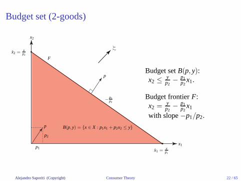
B(p, y) = {x ∈ X : p1x1 + p2x2 ≤ y}

%

F

p

p

p2

p1

Budget setB(p, y):x2 ≤ y

p2− p1

p2x1.

Budget frontierF:x2 = y

p2− p1

p2x1

with slope−p1/p2.


Behavioral assumption: Rationality

So far, we have a model capable of representing consumer’s feasible choicesand his preferences over them.

Now we restrict consumer’s behavior assuming that he is arational agent, inthe sense that he chooses the best alternative in the budget set B(p, y)according with his preference relation%.

Thusrationality in microeconomics has two different meanings:

1. Consumer orders consistently (transitively)all possible alternatives;

2. Consumer chooses the best alternative among those in the feasible set.

We are now ready to study consumer’s optimal choices!


Utility maximizationFormally, consumer’sutility maximization problem(UMP) is

maxx∈X

u(x1, . . . , xn)

s.t.∑n

i=1 pixi ≤ y.(10)

The utility functionu is a real valued and continuous function.

The budget setB is a nonempty (0∈ X), closed, bounded (pi > 0 ∀i) and thusa compact subset ofRn.

Therefore, by the Weierstrass theorem, a maximum ofu overB exists.

Let’s assume the solution of (10), denotedx∗, is interior, i.e.∀i, x∗i > 0; thenUMP can be solved using the Kuhn-Tucker method.

Set up the Lagrange function

L(x1, . . . , xn, λ) = u(x1, . . . , xn) + λ

[

y −n∑

i=1

pixi

]

. (11)


Interior solution (x∗i > 0)

DifferentiatingL(·) w.r.t. each argument, we get the Kuhn-Tuckerfirst orderconditions(FOC’s) at the critical bundlex∗:

∂L(x∗, λ∗)

∂xi=

∂u(x∗)∂xi

− λ∗pi = 0, ∀i = 1, . . . , n, (12)

∂L(x∗, λ∗)

∂λ= y −

n∑

i=1

pix∗

i ≥ 0, (13)

λ∗ ≥ 0, andλ∗ ·

(

y −n∑

i=1

pix∗

i

)

= 0. (14)

Imposing strict monotonicity, (13) must be satisfied with equality, andtherefore (14) becomes redundant.


Interior solution (x∗i > 0)

AssumingMUi(x∗) > 0 for somei, it becomes clear from (12) that

∂u(x∗)∂x1

1p1

=∂u(x∗)∂x2

1p2

= · · · =∂u(x∗)∂xn

1pn

= λ∗ > 0.

Hence, the (absolute value of the) marginal rate of substitution atx∗ betweenany two goods equals the price ratio of those goods:

|MRSij(x∗)| =

MUi(x∗)MUj(x∗)

=pi

pj. (15)

Otherwise, the consumer can improve by substituting a good with a lower MUby a good with a higher MU.

The Lagrange multiplierλ∗ is called theshadow price of money, and it givesthe utility of consuming one extra currency unit.


Interior solution (2 goods)Graphically, in the case of two goods (15) is equivalent to the tangencybetween the highest indifference curve and the budget constraint.

∇u(x∗) = (MU1(x∗),MU2(x

∗))

∇g(x∗) = (−p1,−p2) u∗

x1

x2 FOC: ∇u(x∗)=λ · ∇g(x∗)

g(x∗) = y − p1x∗

1 − p2x∗

2 = 0

x∗

Figure 7:Interior solutionx∗i > 0.


Interior & corner solution (2 goods)

Figure 8:(a) Interior solutionx∗i > 0; (b) Corner solutionx∗i ≥ 0.


Second order conditions

Strictly speaking, for any critical pointx∗ that satisfies the FOCs, we mustcheck that the second order conditions (SOCs) for maxima aresatisfied atx∗.

However, ifu(·) is quasiconcave onRn+ and(x∗, λ∗) ≫ 0 solves the FOCs of

the Lagrange maximization problem, thenx∗ solves (10).

The consumer’s optimal choicesx∗i (p, y), as a function of all pricesp1, . . . , pn

and incomey, are called theWalrasian demands.

N.B. They are also called sometimesMarshallian demands.

From now on, we assumex∗i (p, y) is differentiable.


Example

Let’s find the Walrasian demands for the case in which

u(x1, x2) = (xρ1 + xρ

2)1/ρ, ρ ∈ (0, 1).

Consumer’s utility maximization problem is

max(x1,x2)∈R

2+

(xρ1 + xρ

2)1/ρ

s.t. p1x1 + p2x2 ≤ y.

The associated Lagrange function is

L(x1, x2, λ) = (xρ1 + xρ

2)1/ρ + λ(y − p1x1 − p2x2).

Because preferences are strictly monotonic, the consumer will spend hiswhole budget inx1 andx2.


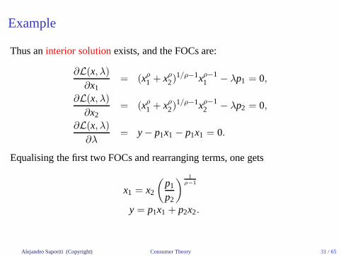
Example

Thus aninterior solutionexists, and the FOCs are:

∂L(x, λ)

∂x1= (xρ

1 + xρ2)

1/ρ−1xρ−11 − λp1 = 0,

∂L(x, λ)

∂x2= (xρ

1 + xρ2)

1/ρ−1xρ−12 − λp2 = 0,

∂L(x, λ)

∂λ= y − p1x1 − p1x1 = 0.

Equalising the first two FOCs and rearranging terms, one gets

x1 = x2

(p1

p2

) 1ρ−1

y = p1x1 + p2x2.


Example

Plugging the first expression into the second, we have

y = p1x2

(p1

p2

) 1ρ−1

+ p2x2 = x2(pρ

ρ−11 + p

ρ

ρ−12 )p

−1

ρ−12 .

Finally, solving forx2 and then forx1, we find that

x∗2(p, y) =yp

1ρ−12

pρ

ρ−11 + p

ρ

ρ−12

and

x∗1(p, y) =yp

1ρ−11

pρ

ρ−11 + p

ρ

ρ−12

.


Indirect utilityThe function mapping out the maximum attainable utility fordifferent pricesand income is called theindirect utility function.

It is defined as

V(p, y) = max

{

u(x1, . . . , xn) :n∑

i=1

pixi ≤ y

}

,

= u(x∗1(p, y), . . . , x∗n(p, y)).

Geometrically,V(p, y) is equal to theutility level associated with thehighest indifference curve theconsumer can achieve with incomeyand at pricesp.


Roy’s identityAn important result in consumer theory, known asRoy’s identity, shows thatthe Walrasian demands can be recovered from the indirect utility.

To be precise, ifV is differentiable at(p, y) and∂V(p, y)/∂y 6= 0, then

x∗j (p, y) = −

∂V(p,y)∂pj

∂V(p,y)∂y

for all j = 1, . . . , n. (16)

The proof of (16) rests on theenvelope theorem.

The envelope theorem states that the effect of changing a parameterαk overthe optimized value of the objective functionv∗ is given by the first-orderpartial derivative of the Lagrange function with respect toαk, evaluated at theoptimal (interior) point(x∗, λ∗).

∂v∗(α)

∂αk=

∂L(x∗, λ∗)

∂αk, k = 1, . . . , l. (17)


Roy’s identity

In the utility maximization problem maxx u(x) s.t. g(x, p, y) = y − p · x = 0,the Lagrange function isL(x, λ) = u(x) + λ(y − p · x). If x∗ ≫ 0,

◮∂V(p,y)

∂pj

(

= ∂L(x∗ ,λ∗)∂pj

)

= −λ∗ · x∗j (p, y); and

◮∂V(p,y)

∂y

(

= ∂L(x∗ ,λ∗)∂y

)

= λ∗ (> 0 cosp ≫ 0 & MUi(x∗) > 0 for somei).

Therefore,

∂V(p,y)∂pj

∂V(p,y)∂y

=−λ∗ · x∗j (p, y)

λ∗= −x∗j (p, y),

which is precisely Roy’s identity.


Marginal utility of income

As noted above, by the Envelope theorem,

λ∗ =∂V(p, y)

∂y.

That is, in the utility maximization problem the Lagrange multiplier is said tobe themarginal utility of income.

Alternatively,λ∗ is also called theshadow priceof (the resource)y.

In words, in the UMP the Lagrange multiplier measures the change of theoptimal value of the utility function as we relax in one unit the budgetconstraint.


Indirect utility’s propertiesAssumingx∗ ≫ 0 andMUi(x∗) > 0 for somei, the indirect utility functionsatisfies the following properties:

For all (p, y) ∈ Rn+1++ , V(p, y) is (i) decreasing inpj, j = 1, . . . , n, and (ii)

increasing iny; i.e., for all(p, y) ∈ Rn+1++ ,

◮∂V(p,y)

∂pj= −λ∗ · x∗j (p, y) < 0, j = 1, . . . , n; and

◮∂V(p,y)

∂y = λ∗ > 0.

For all (p, y) ∈ Rn+1++ , V(p, y) is quasi-convexin prices and income; i.e., for all

(pa, ya), (pb, yb), andβ ∈ (0, 1),

V(p, y) ≤ max{V(pa, ya), V(pb, yb)},

wherep = βpa + (1− β)pb andy = βya + (1− β)yb.


Indirect utility’s propertiesThe intuition as to whyV(p, y) is quasi-convexin prices and income is givenin the following graph.

x1

x2

pa x = ya

pb x = yb

V (pa, ya) = V (pb, yb)

V (p, y)p x = y


Indirect utility’s properties

For all (p, y) ∈ Rn+1++ , V(p, y) is homogeneous of degree zeroin prices and

income; i.e., for all(p, y) ∈ Rn+1++ andα > 0,

V(αp, αy) = V(p, y).

To see this, fix any(p, y) ∈ Rn+1++ andα > 0. By definition,

V(αp, αy) = max{u(x) : (αp) · x ≤ αy}

= max{u(x) : p · x ≤ y}

= V(p, y).

N.B. Bear in mind thatx(αp, αy) = x(p, y); i.e. Walrasian demands arehomogeneous of degree zero in prices and income (no monetary illusion).


Expenditure minimization

Theprimary utility maximizationproblem studied before

maxx∈X

u(x1, . . . , xn)

s.t. p1x1 + · · · + pnxn ≤ y,

has the followingdual expenditure minimizationproblem (EMP)

minx∈X

p1x1 + · · · + pnxn

s.t. u(x1, . . . , xn) ≥ u,

where the utility levelu is maximal at(p, y), i.e., u = V(p, y).

The solution of the EMP gives the lowest possible expenditure to achieveutility u at pricesp.


Expenditure minimizationGraphically, the problem for theutility-maximizing consumeris to movealong the budget liney0 until he achieves the highest ICu0.

The problem for theexpenditure-minimizing consumeris to move along theu0-IC until he reaches the lowest iso-expenditure liney0.



More generally, the minimum expenditure required to attainutility w givenpricesp ∈ R

n++ is found by solving

minx∈R

n+

p · x s.t. u(x) ≥ w. (18)

Note that, forp ≫ 0 andx ∈ Rn+, the set of expendituresp · x that satisfies the

restrictionu(x) ≥ w is closed and bounded below by zero. Therefore, aminimum always exists.

The Lagrange function corresponding to (18) is:

L(x, λ) = −p · x + λ(u(x) − w); (19)

and the Kuhn-Tucker conditions in an interior pointx∗ ≫ 0 are as follows:



1. ∂L(x∗,λ∗)∂xi

= −pi + λ∗ · ∂u(x∗)∂xi

= 0, i = 1, . . . , n;

2. u(x∗) ≥ w;

3. λ∗ ≥ 0 andλ∗ · (u(x∗) − w) = 0.

If p 6= 0, then the constraint must be binding atx∗; i.e.,λ∗ > 0 andu(x∗) = w.

Thus, in the interior solutionx∗ ≫ 0 we have that:

MRSij(x∗) = −

ui(x∗)uj(x∗)

= −pi

pj,∀i 6= j and

u(x∗) = w.


Hicksian demands

The solution to the EMP, denoted byxh(p, w) = (xh1(p, w), . . . , xh

n(p, w)),provides what is known as theHicksian or compensated demands.

xhj (·) depends on pricesp ∈ R

n++ and welfarew ∈ R, as opposite to the

Walrasian demandx∗j (·), that depends on pricesp ∈ Rn++ and incomey > 0.

This is because the Hicksian demands must satisfy the utility constraint,whereas the Walrasian demands must satisfy the budget constraint.

Walrasian demands explain consumer’s observable market demand behavior.

The Hicksian demands instead are not observable (depend on utility!);however, their analytic importance will become evident when we explain theeffect of a price change over the quantities demanded of eachgood.


Expenditure function

The value function of the expenditure minimization problemis called theexpenditure function, and is defined as follows

E(p, u) = min

{n∑

i=1

pixi : u(x1, . . . , xn) ≥ u

}

= p1 xh1(p, u) + . . . + pn xh

n(p, u).

The assumptions 1-5 on consumers’ preferences imply that the expenditurefunctionE(p, u) verifies the following properties:

For every utility levelu ∈ R, E(p, u) is concave inp; i.e., for allp′, p′′, andα ∈ (0, 1),

E(pα, u) ≥ α · E(p′, u) + (1− α) · E(p′′, u),

wherepα = α · p′ + (1− α) · p′′.


Expenditure function’s properties

To see this formally, fixu ∈ R, p′, p′′ ∈ Rn++, andα ∈ (0, 1).

By definition,

E(p′, u) = p′ · xh(p′, u),

E(p′′, u) = p′′ · xh(p′′, u),

E(pα, u) = pα · xh(pα, u).

Sincexh(p′, u), xh(p′′, u), andxh(pα, u) are solutions to theirrespective EMPs

£

p′

E(p′, u) = p′ xh(p′, u)p′ xh(pα, u)

pα

E(pα, u) = pα xh(pα, u)

p′′ p

E(p′′, u) = p′′ xh(p′′, u)

p′′ xh(pα, u)p xh(p′′, u)

E(p, u)

p xh(p′, u) p xh(pα, u)

p′ · xh(p′, u) ≤ p′ · xh(pα, u), (20)

andp′′ · xh(p′′, u) ≤ p′′ · xh(pα, u). (21)



If we multiply (20) byα and (21) by(1−α), and we add the inequalities, then

αp′ · xh(p′, u) + (1− α)p′′ · xh(p′′, u) ≤ [αp′ + (1− α)p′′] · xh(pα, u),

≤ pα · xh(pα, u).

Therefore,α · E(p′, u) + (1− α) · E(p′′, u) ≤ E(pα, u).

(Shephard’s Lemma)The Hicksian demands are equal to the partialderivatives of the expenditure function with respect to theprices; i.e., for allj = 1, . . . , n, and all(p, u) ∈ R

n++ × R,

xhj (p, u) =

∂E(p, u)

∂pj.



The proof rests on the Envelope theorem.

The Lagrange function associated to the EMP minx p · x subject tou(x) − u ≥ 0 is L(x, λ) = p · x + λ[u − u(x)], (with λ > 0 cosp ≫ 0).

Hence, using (17), we get the Shephard’s Lemma:

∂E(p, u)

∂pi=

∂L(x∗, λ∗)

∂pi= xh

i (p, u). (22)

N.B. The pair(x∗, λ∗) in (22) denotes the interior solution of the EMP.

Intuitively, Shephard’s Lemma says the following. SupposePeter buys 12units ofxi at $1 each. Assume thatpi increases to $1.1.



Shephard’s lemma says that, tomaintain utilityu constant, theexpenditure must increase by∆E = xi · ∆pi = 12 · 0.1 = $1.2(if xi doesn’t change!).

SinceE(p, u) is concave inp,xi · ∆pi overstates the requiredincrease (cosxi actually changeswhenpi changes).

But, for ∆pi small enough, thedifference can be ignored.



Givenu ∈ R, for all i = 1, . . . , n, E(p, u) is increasing inpi; i.e., ∂E(p,u)∂pi

> 0,

with strict inequality becausexhi (p, u) > 0 (interior solution).

This property follows from (22); it simply means that higherprices⇒ agreater expenditure is needed to attainu.

If there exists an interior solution for the expenditure minimization problem,then by the Envelope theorem,

∂E(p, u)

∂u= λ∗ > 0.

Hence, givenp ∈ Rn++, E(p, u) is increasing inu.

In the EMP the Lagrange multiplier represents the rate of change of theminimized expenditure w.r.t. the utility target, i.e.,the utility’s marginal cost.



Givenu ∈ R, E(p, u) is homogeneous of degree one inp.

To see this, note that Hicksian demands are homogeneous of degree zero inprices; i.e., for all(p, u) and allk > 0, xh(kp, u) = xh(p, u).

The reason is any equi-proportional change in all prices does not alter theslope of the iso-expenditure curves!

Therefore, givenu ∈ R, for all p ∈ Rn++ andk > 0,

E(kp, u) = (kp) · xh(kp, u) = k(p · xh(p, u)) = k · E(p, u).


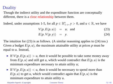
DualityThough the indirect utility and the expenditure function are conceptuallydifferent, there is aclose relationshipbetween them.

Indeed, under assumptions 1-5, for allp ∈ Rn++, y > 0, andu ∈ R, we have

V(p, E(p, u)) = u; and (23)

E(p, V(p, y)) = y. (24)

The intuition for (23) is as follows. (A similar reasoning applies to (24) too.)Given a budgetE(p, u), the maximum attainable utility at pricesp must beequal tou. Instead,

◮ If V(p, E(p, u)) > u, then it would be possible to take some money awayfrom E(p, u) and still getu, which would contradict thatE(p, u) is theminimum expenditure necessary to attain utilityu;

◮ If V(p, E(p, u)) < u, then it would be necessary to spend more thanE(p, u) to getu, which would contradict again thatE(p, u) is theminimum expenditure to attain utilityu.


DualityThe relationships stated in (23) and (24) indicate that we don’t need to solveboth UMP and EMP to find the indirect utility and the expenditure function.

From (23), holding pricesp constant, we can invertV(p, ·) to get

E(p, u) = V−1(p, u). (25)

Notice thatV−1(p, ·) exists becauseV(p, ·) is increasing in income.

Similarly, from (24), holdingp fixed, we can invertE(p, ·) to get

V(p, y) = E−1(p, y). (26)

Notice thatE−1(p, ·) exists becauseE(p, ·) is increasing in utility.

Formally, (25) and (26) reflect that the indirect utility andthe expenditurefunction are simply the appropriately chosen inverses of each other.


Duality

In view of this, it is natural to expect a close relationship between theHicksian and the Walrasian demands too.

In effect, for allp ∈ Rn++, y > 0, u ∈ R, andi = 1, . . . , n, we have

x∗i (p, y) = xhi (p, V(p, y)); and (27)

xhi (p, u) = x∗i (p, E(p, u)). (28)

◮ (27) says that the Walrasian demand at pricesp and incomey is equal tothe Hicksian demand at pricesp and the maximum utility at(p, y);

◮ (28) says that the Hicksian demand at pricesp and utility u is equal to theWalrasian demand at pricesp and the minimum expenditure at(p, u).


Duality

Another way to read (27) and (28) is the following.

◮ If x∗ solves maxu(x)s.t. p · x ≤ y, thenx∗

solves min(p · x) s.t.u(x) ≥ u∗ ≡ u(x∗);

◮ Conversely, ifx∗

solves min(p · x) s.t.u(x) ≥ u, thenx∗

solves maxu(x) s.t.p · x ≤ y∗ ≡ p · x∗.

u = u(x∗) = V (p, y)

x1

x2

x∗(p, y) = xh(p, V (p, y))

y/p1

y/p2

E(p, u)

xh(p, u) = x∗(p, E(p, u))

For that reason, we sayx∗ has adualnature.


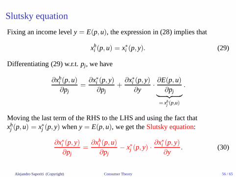
Slutsky equation

Fixing an income levely = E(p, u), the expression in (28) implies that

xhi (p, u) = x∗i (p, y). (29)

Differentiating (29) w.r.t.pj, we have

∂xhi (p, u)

∂pj=

∂x∗i (p, y)∂pj

+∂x∗i (p, y)

∂y·∂E(p, u)

∂pj︸︷︷︸

= xhj (p,u)

.

Moving the last term of the RHS to the LHS and using the fact thatxh

j (p, u) = x∗j (p, y) wheny = E(p, u), we get theSlutsky equation:

∂x∗i (p, y)∂pj

=∂xh

i (p, u)

∂pj− x∗j (p, y) ·

∂x∗i (p, y)∂y

. (30)


Slutsky equation

The Slutsky equation is sometimes called thefundamental equation ofdemand theory.

If we differentiate (29) w.r.t. the own-pricepi, then (30) tells us that the slopeof the Walrasian demand is the sum of two effects:

◮ An unobservablesubstitution effect, ∂xhi (p, u)/∂pi, given by the slope of

the Hicksian demand; and

◮ An observableincome effect, −x∗i (p, y) · [∂x∗i (p, y)/∂y];

∂x∗i (p, y)∂pi

=∂xh

i (p, u)

∂pi︸︷︷︸

SE

− x∗i (p, y) ·∂x∗i (p, y)

∂y︸︷︷︸

IE

.


Slutsky decomposition

x1

s

x2

s

s

x1

x2

%

xa(p1, p2, y)xa

2

xa1

B(p1, p2, y)

u∗(p1, p2, y)

Initial choicexa given pricespand incomey.


Slutsky decomposition: Substitution effect

x1

s

s

x1

x2

%

xb(p′1, p2, y′)

xa(p1, p2, y)xa

2

xa1 xb

1

B(p1, p2, y) B(p′1, p2, y)

u∗(p1, p2, y)

xb2

SE

SE B(p′1, p2, y′)

Reduce pricep1 to p′1, but keepthe consumer on the sameindifference curve.


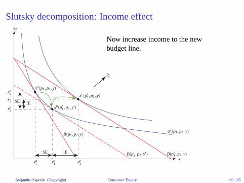
Slutsky decomposition: Income effect

x1

s

s

x1

x2

%

xb(p′1, p2, y′)

xa(p1, p2, y)xa

2

xa1 xb

1

B(p1, p2, y)

B(p′1, p2, y)

u∗(p1, p2, y)

xb2

xc1

xc2 SE

SE

IE

IE B(p′1, p2, y′)

xc(p′1, p2, y)

Now increase income to the newbudget line.


Upshot from the Slutsky decomposition

A price change has two effects

◮ substitution effect: always negative, and

◮ income effect: cannot be signed—depends on preferences.

Depending on the sum of these two effects, (Walrasian) demand may changeeither way following a price reduction.

However, we know that

◮ If ∂x∗i /∂y > 0 (normal good), SE and IE goes in the same direction andthe Walrasian demand has a negative slope;

◮ If ∂x∗i /∂y < 0 (inferior good), the sign of the slope of the Walrasiandemand depends on the size of|∂xh

i /∂pi| in relation to|x∗i · ∂x∗i /∂y|.


Slutsky matrixConsider then × n-matrix of first-order partial derivatives of the Hicksiandemands:

σ(p, u) =

∂xh1(p,u)∂p1

. . .∂xh

1(p,u)∂pn

..... .

...∂xh

n(p,u)∂p1

. . .∂xh

n(p,u)∂pn

.

By Shephard’s Lemma,σ(p, u) is the matrix of second-order partialderivatives of the expenditure function, which is concave in prices. Thus,σ(p, u) is negative semi-definite.

Moreover, by definition of negative semi-definiteness, the elements of thediagonal are non-positive; i.e.

∂xhi (p, u)

∂pi=

∂2E(p, u)

∂p2i

≤ 0. (31)


Demands’ slopesThat means the Hicksian demands cannot have a positive slope!

Finally if E(p, u) is twice continuously differentiable,σ(p, u) is symmetricbecause Young’s theorem implies

∂xhi (p, u)

∂pj=

∂xhj (p, u)

∂pi.

Assuming that the Walrasian demand forxi is also downward sloping, therelationship between the slopes is as follows.

For a normal good:

◮ Whenpi ↓, Walrasian↑ more than Hicksian because IE reinforces SE;

◮ Equally, whenpi ↑, Walrasian↓ more than Hicksian because IEreinforces SE.


Demands’ slopes: normal goodAs a result,Walrasian demand is flatter than Hicksian demand whenxi is anormal good.

xi

pi

xhi (p, V (p, y))

x∗

i (p, y)

p′′i

pi

p′i

a b c d


Demands’ slopes: inferior goodFor an inferior good:

◮ Whenpi ↓, Walrasian↑ less than Hicksian because IE offsets part of theSE;

◮ Equally, whenpi ↑, Walrasian↓ less than Hicksian because IE offsetspart of the SE.

As a result, assuming both havenegative slopes,Hicksiandemand is flatter than Walrasiandemand whenxi is an inferiorgood.

xi

pi

xhi (p, V (p, y))

x∗

i (p, y)

p′′i

pi

p′i

a b c d


notes on consumer theory - university of manchester · title: notes on consumer theory author:...

Documents