norc at the university of chicago the university of...
TRANSCRIPT

NORC at the University of ChicagoThe University of Chicago
Competition and the Ratchet EffectAuthor(s): Gary Charness, Peter Kuhn, and Marie Claire VillevalSource: Journal of Labor Economics, Vol. 29, No. 3 (July 2011), pp. 513-547Published by: The University of Chicago Press on behalf of the Society of Labor Economists andthe NORC at the University of ChicagoStable URL: http://www.jstor.org/stable/10.1086/659347 .
Accessed: 25/07/2014 17:13
Your use of the JSTOR archive indicates your acceptance of the Terms & Conditions of Use, available at .http://www.jstor.org/page/info/about/policies/terms.jsp
.JSTOR is a not-for-profit service that helps scholars, researchers, and students discover, use, and build upon a wide range ofcontent in a trusted digital archive. We use information technology and tools to increase productivity and facilitate new formsof scholarship. For more information about JSTOR, please contact [email protected].
.
The University of Chicago Press, Society of Labor Economists, NORC at the University of Chicago, TheUniversity of Chicago are collaborating with JSTOR to digitize, preserve and extend access to Journal ofLabor Economics.
http://www.jstor.org
This content downloaded from 128.111.121.42 on Fri, 25 Jul 2014 17:13:52 PMAll use subject to JSTOR Terms and Conditions
513
[Journal of Labor Economics, 2011, vol. 29, no. 3]� 2011 by The University of Chicago. All rights reserved.0734-306X/2011/2903-0003$10.00
Competition and the Ratchet Effect
Gary Charness, University of California, Santa Barbara
Peter Kuhn, University of California, Santa Barbara
Marie Claire Villeval, University of Lyon 2, CNRS-GATE
In labor markets, the ratchet effect refers to a situation whereworkers subject to performance pay choose to restrict their out-put, because they rationally anticipate that firms will respond tohigher output levels by raising output requirements or by cuttingpay. We model this effect as a multiperiod principal-agent problemwith hidden information and study its robustness to labor marketcompetition both theoretically and experimentally. Consistentwith our theoretical model, we observe substantial ratchet effectsin the absence of competition, which are nearly eliminated whencompetition is introduced; this is true regardless of whether mar-ket conditions favor firms or workers.
We would like to acknowledge Bentley MacLeod for useful discussions thathelped to inspire this paper, and David Cooper, Werner Guth, Bernard Salanie,and seminar participants at the European meeting of the Economic ScienceAssociation in Lyon, at the Third European Workshop on Experimental andBehavioral Economics in Innsbruck, at the conference of the European Asso-ciation of Labour Economists in Tallin, at the Beijing Normal University, atICES at George Mason University in Washington, DC, and at the Universitiesof Toulouse, Rennes, Nancy, Tilburg, and Xiamen for helpful comments. Wewould also like to thank Julie Rosaz for valuable research assistance. Kuhnthanks UC Berkeley’s Center for Labor Economics for their generous hospi-tality while conducting research on this project. Villeval gratefully acknowledgesfinancial support from the EMIR program at the French National Agency forResearch (ANR BLAN07-3_185547).
This content downloaded from 128.111.121.42 on Fri, 25 Jul 2014 17:13:52 PMAll use subject to JSTOR Terms and Conditions

514 Charness et al.
Most of the work in one of the largest tire-building plants inthe country is on a piece-rate basis. In one department, thepiece workers pushed their earnings up to $12 a day. Said anemployee in this department, “The rate was immediately cut.Now we know that the maximum paid for this work is $7 aday. It would be possible for us to do much more but we arecareful not to.”
And a girl who was experienced in a wide range of employmentexplained: “I have learned through sad experience that the moreyour superiors find they can get out of you the more theycome to expect. The only way to protect yourself is never towork at anything like full capacity. I know that most restrictionis due to the worker’s desire to save and protect herself andnot to any other motive.” (Quotes are from Mathewson [1931,chap. 3])
I. Introduction
While piece rates and other forms of performance-based pay have beenused successfully in many contexts (e.g., Lazear 2000), one potential prob-lem affecting such schemes, labeled the “ratchet effect,” has been rec-ognized since at least the 1930s. At that time, industrial sociologists likeStanley Mathewson found that piece-rate workers were often careful tolimit their output. On the basis of bitter experience, such workers wereconfident that choosing a higher output might yield short-term gains butwould soon result in either a cut to their rate or an increase in productionquotas that would leave them worse off in the long run. Thus, in contrastto the predictions of a static model (such as Lazear’s), piece rates mightactually reduce worker performance when workers consider the dynamicimplications of current effort choices.
To the best of our knowledge, formal models of ratchet effects did notemerge until shortly after the development of asymmetric-informationmodels of principal-agent interactions in the early 1980s. At that time, itwas recognized that these effects can be modeled as a situation where aprincipal contracts with an agent more than once, the agent takes a non-contractible action and has private information, and binding multiperiodcontracts are not enforceable (Freixas, Guesnerie, and Tirole 1985). Insuch situations, actions taken by the agent early in the relationship canreveal information to the principal, who then uses the information to theagent’s disadvantage. In addition to the economics of worker incentiveswithin firms (Gibbons 1987; Ickes and Samuelson 1987; Carmichael andMacLeod 2000), other interactions that have been modeled using a ratcheteffect framework include the setting of production targets for branchesof a multidivisional firm or a nationalized economy (Weitzman 1980),
This content downloaded from 128.111.121.42 on Fri, 25 Jul 2014 17:13:52 PMAll use subject to JSTOR Terms and Conditions

Competition and the Ratchet Effect 515
contracting between a social-welfare–maximizing regulator and firms un-der his or her jurisdiction (Laffont and Tirole 1988; Litwack 1993; Dalen1995), managers’ incentives to innovate (Dearden, Ickes, and Samuelson1990), procurement contracting (Laffont and Tirole 1993), optimal incometaxation (Dillen and Lundholm 1996), the economics of corruption (Choiand Thum 2003), and environmental regulation (Puller 2006).
A common feature of the above models is the presence of poolingequilibria early in the principal-agent relationship. For example, in thecase of worker compensation, abler workers tend to mimic workers withless talent (or to act “as if” the firm’s technology is less productive thanit truly is) by restricting their output early in the employment relationship.This benefits abler workers (or workers lucky enough to discover thatthe production technology is “good”) by preventing the firm from ex-tracting their rents later in the relationship, but it is socially inefficient.Another, less well-known feature of existing ratchet models is their ten-dency to model agents’ participation constraints very simply, typically byrequiring the utility of all agent types to exceed the same threshold ineach period. While this may make sense in some cases, we see it as ap-plicable to labor markets only in cases where market frictions are high;essentially, workers’ only alternative to their current match is modeled asan activity (such as unemployment) that is equally valuable to all workers,no matter how able they are. The option of putting one’s talents to workat another firm with the same technology as the current one is typicallynot modeled.
The robustness of the ratchet effect to the competitive environmentthus strikes us as an important but understudied question, in both laboreconomics and the economics of incentives and information more gen-erally. For example, while ratchet effects may be common in labor marketscharacterized by substantial mobility costs or firm-specific capital, theimportance of ratchet effects in markets characterized by a high degreeof competition and (at least potential) mobility is less clear. One modelof ratchet effects that expands the treatment of agents’ labor market al-ternatives is the one designed by Kanemoto and MacLeod (1992).1 Ka-nemoto and MacLeod show that, even when the labor market does notobserve the agent’s early career performance, the presence of ex post
1 Another such model is that of Roland and Sekkat (2000), who consider asituation where agents’ first-stage performance is observed by an outside labormarket. Arguably, this puts the Roland-Sekkat model into a different class ofmodels from the ratchet-effect literature, often referred to as “career-concerns”models (see, e.g., Dewatripont, Jewitt, and Tirole 1999). In addition to makingagents’ output public information, career-concerns models typically do not in-corporate private information about an agent’s type. In contrast to ratchet-effectmodels, career-concerns models are capable of generating socially excessive effortearly in the agent’s career.
This content downloaded from 128.111.121.42 on Fri, 25 Jul 2014 17:13:52 PMAll use subject to JSTOR Terms and Conditions

516 Charness et al.
market opportunities for agents can eliminate the ratchet effect, allowingfirst-best effort levels to be attained.2 This suggests that ex post marketsfor agents may be a more powerful force in eliminating ratchet effectsthan previously realized.
While numerous case studies, including the famous Lincoln Electriccase discussed by Carmichael and MacLeod (2000), strongly suggest thatratchet effects can be important in real workplaces, such effects are difficultto study econometrically or using field experiments. Theoretically, ratcheteffects are predicted to occur in specific informational and contractualenvironments; both hidden action and hidden information must be pre-sent, and the parties must be in a repeated relationship yielding somequasi-rents to both parties where binding multiperiod agreements are notfeasible. Measuring and either manipulating or isolating plausibly exog-enous natural variation in these features of the environment presents sig-nificant challenges. Taking the additional step of manipulating the amountof labor market competition affecting workers and firms, which is thefocus of this paper, adds to these challenges. On the other hand, all ofthese economic, informational, and contractual features can be preciselymeasured and exogenously manipulated in the laboratory.
Given the above discussion, it is not surprising that—aside from thecase studies discussed above—the only empirical evidence of ratchet ef-fects we know of is experimental in nature.3 Chaudhuri (1998) conducteda laboratory experiment in which principals and agents interacted for twoperiods, and agents were one of two types that were unobserved by theprincipal. There was little evidence of ratcheting; most agents played na-ively, revealing their type in the first period even when an informed prin-cipal would use this information to the agent’s disadvantage, and principalsoften did not exploit agents’ type revelation. Possible explanations forthis result include the relative complexity of the game and the lack ofcontext provided to the subjects that might have impeded the learningprocess.
The only other experimental study of the ratchet effect of which weare aware is the study by Cooper et al. (1999). Cooper et al. frame their
2 Intuitively, this is because abler agents are able to generate more total surplusfrom the employment relationship than less-able agents. Even when the marketdoes not observe first-stage performance, this generates type-specific participationconstraints in the second stage, which protect abler agents from exploitation. Notethat this reasoning does not apply to the case modeled by Gibbons (1987), wherethe asymmetric information applies to the firm’s technology rather than the agent’stype.
3 An exception is Allen and Lueck (1999), who use cash rent and crop-sharecontract data to test for the presence of the ratchet effect in the context of moralhazard in agricultural contracts but do not consider the role of competition. Theyfind limited evidence for the ratchet effect within share contracts and concludethat it cannot explain the choice of contracts.
This content downloaded from 128.111.121.42 on Fri, 25 Jul 2014 17:13:52 PMAll use subject to JSTOR Terms and Conditions

Competition and the Ratchet Effect 517
experiment in a context-rich way (as a game between central planners andfirm managers), use both students and actual Chinese firm managers assubjects, and implement experimental payoffs with high stakes relative tothe participants’ real-world incomes. They also simplify the interactionsbetween principals and agents, focusing the experiment only on the stagesof the game where information revelation matters: the agent’s effort choicein the first period and the principal’s choice of a payoff schedule in thesecond. Cooper et al. do find evidence of ratchet effects, although evenin their context it took some time for the players to learn the consequencesof type revelation. Their artefactual field experiment with managers sup-ports the external validity of ratchet effects found in the laboratory.
This paper reports the results of some simple laboratory experimentson the ratchet effect, in the context of piece-rate compensation. It differsfrom existing experimental studies in two main ways. First, motivated byour discussion of competition above and by Kanemoto and MacLeod’stheoretical insight, our study is the first to introduce market competitionfor agents and principals, by allowing players to choose between theircurrent partner and an alternative partner at the start of each stage of thegame.4 Second, motivated by the experimental approach of Cooper et al.,we simplify the interactions between principals and agents even further.Specifically, we focus only on the strategic interactions at the heart of theratchet effect (i.e., those between the high-talent agents’ first-stage effortsand the principals’ second-stage rewards), and we reduce both parties’strategy sets to two choices (high or low output, and high or low pay).Combining this with a simple context that makes sense to our subjects(principals are firms and agents are workers), we believe that this signif-icantly improves our subjects’ understanding of the game.
Our main findings are twofold. First, we observe substantial and sig-nificant ratchet effects in the baseline case of our model (which, like thestudies by Chaudhuri and Cooper et al., does not incorporate labor marketcompetition). We believe that this is in large part due to our simple designthat focuses on the main strategic issues. Second, we find that ratchetbehavior is significantly reduced by competition; interestingly, this is trueregardless of whether market conditions favor workers (our “excess firms”
4 We are aware of only two other principal-agent experiments that includetreatments featuring both excess firms and excess workers. Brandts and Charness(2004) find only minor effects on the ratio of “effort” to “wage,” according tothe direction of market imbalance in a gift-exchange experiment, and also finddeleterious effects on effort when a minimum wage is introduced. Cabrales, Char-ness, and Villeval (forthcoming) show that in a static game with informationalasymmetry and hidden information, inefficiencies remain when principals competeagainst each other to hire agents. In contrast, when agents compete to be hired,efficiency improves dramatically, and it increases in the relative number of agentsbecause competition reduces the agents’ informational monopoly power.
This content downloaded from 128.111.121.42 on Fri, 25 Jul 2014 17:13:52 PMAll use subject to JSTOR Terms and Conditions

518 Charness et al.
case) or firms (our “excess workers” case). In the excess firms case, itappears (as Kanemoto and MacLeod’s analysis predicts, and consistentwith the Perfect Bayesian Nash equilibrium [PBNE] of the game playedby our subjects) that talented workers are willing to reveal their types inthe first stage, because market alternatives allow them to escape the in-cumbent firm’s desire to exploit them ex post. In the excess workers case(again, consistent with the two pure-strategy PBNE of the game), mosttalented workers once again are willing to reveal their type in the firststage. Now this is because they are no longer assured of remaining em-ployed with the same firm in the second stage; this matching uncertaintyreduces the returns to concealment.
Taken together, while the precise game played by our subjects is hardlygeneral, we conjecture that our results illustrate two simple, general prin-ciples regarding the effects of competition on ratchet effects, both in labormarkets and more generally. First, an improvement in either party’s out-side options (which, holding the other party’s outside options fixed, nec-essarily reduces the quasi-rents associated with the parties’ relationship)tends to reduce the effect that information revelation can have on thepayoffs of the informed party. Since the difference in the agent’s payoffswhen the principal thinks the agent is a “high” type and when the principalthinks the agent is a “low” type is smaller when competition is present,the informed party’s incentives to conceal private information are reduced.Second, informed parties’ incentives to conceal private information arereduced whenever there is turnover in equilibrium; there is no point inmaking a costly investment to conceal private information from someonewith whom one is unlikely to interact in the future.5 Thus, it appears thateither institutional barriers to competition among both agents and prin-cipals, or a high level of labor market frictions, may be more importantto the existence of ratchet effects than previously realized.
II. A Model
Let worker utility be given by , where is total com-U p w � gV(e) wpensation and is the cost of effort, .6 Here has the usual formgV(e) e V(e)
5 Ickes and Samuelson (1987) and Dearden et al. (1990) show theoretically thatan ex ante commitment by an employer with market power to transfer employeesbetween jobs can reduce ratchet effects when hidden productivity is job-specific.While similar in some aspects to our theoretical and empirical result about turn-over, we note that our result applies to hidden information about worker pro-ductivity, and that turnover is an ex post optimal response to market competitionrather than an ex ante commitment in our setup.
6 We focus on a single-task principal-agent setting throughout the paper. Theentire analysis generalizes in a straightforward manner to a multitask setting ifthe principal can observe a sufficient statistic for the agent’s performance on alltasks. If this is not the case, optimal incentives may be zero or very weak (Farrell
This content downloaded from 128.111.121.42 on Fri, 25 Jul 2014 17:13:52 PMAll use subject to JSTOR Terms and Conditions
Competition and the Ratchet Effect 519
[ ]; we use to generate parameter val-′ ′′ 2V(0) p 0, V 1 0, V 1 0 V(e) p eues for the experiment. There are two types of workers, high and lowability (or “talent”), differentiated by their effort costs, . OutputH Lg ! g
is given by the production function ; since this is the same for bothy p eworkers, we henceforth use exclusively to denote both output and effort.yFirms’ profits are given by . Firms offer piece rate contractsP p y � wof the form to workers. In fact, we set , since thisw p �a � by b p 1achieves the first best in a full-information environment. This means thatfirms’ only decision is over the value of . One interpretation ofa a ≥
is as the rental fee the firm charges the worker for the right to use its0plant and equipment; as is well known when , these fees will con-b p 1stitute the firm’s only source of profit.7
Under the above conditions, the socially optimal output levels are givenby . With , these are also the output levels that we expecty p 1/ (2g) b p 1workers to choose in a one-stage interaction with firms, as long as thelevel of satisfies both workers’ participation constraints. High-talenta
workers will produce more output than low-talent workers; in conse-quence, both workers’ types are revealed and a first-best outcome is at-tained.
Now imagine that workers and firms engage in a two-stage interaction,with stages of potentially different length. The worker’s type is still un-known to the firm at the start of the first stage, but the firm now mightinfer something about it from the worker’s stage 1 output. In particular,high stage 1 output might signal high worker talent, implying that thefirm can charge a higher rental fee in stage 2 without violating the worker’sparticipation constraint. Anticipating this, high-talent workers might“masquerade” as low-talent workers in the first stage. As a result, firmswill continue to offer the low rental fee in the second stage, since theywere unable to identify the worker’s type in the first stage. Thus, wewould observe inefficient pooling at the low-output level in the first stage,especially if the first stage is short relative to the second. Finally, supposethat at the start of the second stage all workers can receive a competingwage offer from another firm. As Kanemoto and MacLeod (1992) have
and Shapiro 1989) in which case ratchet effects will not occur. As we have alreadynoted, ratchet effects are, in some sense, an unintended consequence of perfor-mance pay systems; thus they are unlikely to be an issue when performance payis not an important component of compensation.
7 Although explicit job “rental” or entry fees are rarely observed in reality (andare in some cases illegal), it is well known that a variety of contracting mechanismsare equivalent to these fees. One example is a positive level of base compensationcombined with a minimum output quota that must be reached in order to qualifyfor a piece rate; in this interpretation, a higher rental fee (a) corresponds to ahigher output quota. Note also that the 100% piece rates assumed refer to 100%of the firm’s net revenues, not of gross sales. See Lazear (1998, chap. 5) for adiscussion.
This content downloaded from 128.111.121.42 on Fri, 25 Jul 2014 17:13:52 PMAll use subject to JSTOR Terms and Conditions

520 Charness et al.
shown, this can prevent “incumbent” firms from exploiting high-talentworkers who reveal their type in the first stage, even when outside firmsdo not observe workers’ stage 1 outputs. Our experiment tests this pre-diction, implementing the exact model described above with parametervalues as described below.8 As noted, we also test the effect of firms’options to hire alternative workers.
In our experiment, we set and , which yieldsL Hg p 0.010 g p 0.005socially optimal output levels of [ ] 50 and 100 for the low- and1/ (2g) phigh-talent workers, respectively. Throughout the experiment, we restrictworkers’ output choices to these two levels, which we call “low” and“high” output. Thus, if each worker type chooses his “type-appropriate”output, a first-best outcome will be achieved. Asymmetric information-induced inefficiencies will take the form of workers choosing the type-inappropriate output level.
Workers receive a baseline payoff of zero if they do not work for anyfirm. If workers choose type-appropriate outputs, the total surplus gen-erated by the employment relationship [ ] is 25 and 50, respec-e � gV(e)tively, for the low- and high-talent workers; 25 and 50 are thus the max-imum rental fees the firm can charge each type of worker if it knows theworker’s type. In our experiment, we allow firms to choose between tworental fees only: (low) and (high).9 We set the ex anteL Ha p 15 a p 33probability that a worker has high talent at .10 Finally, in our imple-1/3mentation, workers and firms interact over either one or two stages, withthe second stage twice as “long” as the first (thus, all the payoffs listed
8 Kanemoto and MacLeod’s model allows for a much more general menu ofcontracts than is feasible to implement in a laboratory experiment; nevertheless,the same fundamental factors explain the effect of competition on the ratcheteffect in their model as in our simpler version.
9 Most theoretical treatments of principal-agent and ratchet problems appearto assign all the bargaining power to principals, in the sense that equilibriumcontracts are assumed to maximize the principal’s utility subject to the agent’sparticipation constraint. In most contexts this is only apparent, however, sincethis approach is simply a mathematical device for finding a Pareto-optimal con-tract. We take a different approach here by simply dividing the rents between thetwo parties in a way that ensures both will want to participate. Aside fromrealism—it seems likely that bargaining will lead to rent sharing in most cases—allocating a nonzero share of the surplus to both parties has a practical purposein our experiment: allowing firms to make “take-it-or-leave-it” offers that claimthe entire surplus would introduce ultimatum-game effects that are beyond thescope of the current paper.
10 If this probability is too high, a firm that does not know its worker’s typewill optimally choose the high rental fee, thereby shutting low-talent workersout of the market. Thus, in this case the pooling equilibrium at the heart of theratchet model cannot exist, given our payoff parameters. A value of 1/3 givesfirms adequate incentives to set the low fee and retain both worker types whenthe worker’s type is unknown.
This content downloaded from 128.111.121.42 on Fri, 25 Jul 2014 17:13:52 PMAll use subject to JSTOR Terms and Conditions
Competition and the Ratchet Effect 521
above are doubled, and the rental fees adjusted accordingly to 30 and 66).As noted, raising the relative importance of the second stage raises work-ers’ incentives to manipulate the information the firm has about them inthat stage, making ratchet effects more likely.11
Under the above assumptions, low-talent workers’ stage-one payoffsif the firm posts the low rental fee are 10 and �15 at low- and high-effortlevels, respectively; if the firm posts the high fee, they are �8 and �33.Thus, in a one-shot game with no strategic interactions, we expect low-talent workers to choose low effort if the firm posts the low rental fee,and to refuse to work for the firm at the high rental fee. Similar calculationsshow that high-talent workers find it optimal to supply high effort re-gardless of the rental fee (although they are obviously better off at thelow fee). Their stage-one payoffs are 22.5 and 35 at low and high effortlevels, respectively, if the fee is low, and 4.5 and 17 if the fee is high. Thus,we would expect to observe an efficient separating equilibrium if the gamehas only one stage. However, in a two-stage game with no competition—the baseline case in our experiment, and the case studied most frequentlyin the theoretical literature—a forward-looking high-talent worker willconceal his type in the first stage (thus sacrificing some current payoff)if he believes this will lead the firm to charge a lower second-stage fee,leading to an inefficient pooling equilibrium. In terms of pure strategies,this is demonstrated formally in appendix A, which demonstrates thatseparating equilibria do not exist in this situation, while the pooling equi-librium does.12
Appendix A also characterizes the PBNE in our laboratory experimentwhen we introduce competition between firms or between workers.Briefly, appendix A shows that pooling equilibria cannot exist in eitherthe excess firms or the excess-agents treatments. We also show that equi-libria in which agents’ first-stage behavior fully reveals their type do existin both cases (there is a unique PBNE in the excess firms treatment andtwo PBNE in the excess workers treatment). The precise structure ofthose equilibria and the intuition behind them is discussed in more detailin the following section.
11 The vast majority of theoretical ratchet effect models have only two periods;a noteworthy exception is Weitzman’s (1980) infinite-horizon treatment. AsWeitzman’s analysis makes clear, what is important for the size of the ratcheteffect is not the number of periods but simply the importance of the future atany given time (in his case this reduces to the discount rate). We conjecture buthave not proved that equilibrium in finite horizon ratchet models with more thantwo periods involves a transition from pooling in early periods to separation inlater ones.
12 Unless otherwise specified, we confine our discussion of predicted equilibriato pooling and separating equilibria in pure strategies. Thus, we generally omitthe qualifier “in pure strategies” unless we make specific reference to mixed strat-egies.
This content downloaded from 128.111.121.42 on Fri, 25 Jul 2014 17:13:52 PMAll use subject to JSTOR Terms and Conditions

522 Charness et al.
III. Experimental Design
Our experiment was conducted at the Groupe d’Analyse et de TheorieEconomique (GATE), CNRS, France. The students were recruited fromundergraduate courses in local engineering and business schools, by meansof ORSEE software (Greiner 2004). In total, 159 people took part in thenine sessions (three for each treatment) of this experiment. Each partic-ipant was assigned a computer upon arrival, by a draw from an opaquebag. No one could participate in more than one session, and the sameexperimenters conducted all of the sessions. In each treatment, there wasa conversion rate of 100 experimental units to i1. Average earnings werei14, including a i5 show-up fee.
Each participant was given the role of either a high-talent worker or afirm. The number of participants allocated to each category depended onthe treatment. We decided to have automated low-talent workers, as theirdecisions were quite trivial (reject contracts with a high rental fee, as thiswould generate negative earnings for the worker, and accept contractswith low rental fees, since this provides positive earnings for both firmsand workers).13 Since we expected virtually no deviation from this strategy,we programmed the low-talent workers to follow it. It was made commoninformation in the instructions that the low-talent workers were robotsand that they were programmed to follow this strategy.14
In order to facilitate comprehension, we couched our experiment interms of the firm being the owner of a food concession stand on campus.15
Note that the firm’s income is only what is received in rental fees. In thefirst part of a period, the firm is willing to rent the stand (to a worker)for 1 week; we restrict the firm to charging the low rental fee of 15 inorder to provide a high-talent worker with a real choice, thus enablingus to gather useful data.16 If a firm or a worker does not end up in acontractual relationship, he or she receives nothing for that stage. If ahigh-talent worker accepts a contract, he or she chooses either low or
13 Even negative reciprocity could not come into play with human low-talentworkers, as the firm is clearly not being antagonistic by choosing the lower rentalfee.
14 The robots were programmed with different response times and a sessionproceeded to the next step only once all the players had entered their decisions.Therefore, the only evidence that a firm had concerning the nature of the workerwas the choice made by the worker.
15 We attempted to ensure comprehension by requiring participants to completea “Comprehension questionnaire,” which can be found in the online appendixB, along with a sample of the experimental instructions.
16 Choosing the high fee of 33 gives an expected gain of only 11 for the firmin that stage. In addition, allowing the firm to choose the high fee in this stagemight allow it to uncover the type of its worker but at the risk of having its offerrejected if matched with a low-talent worker. This would not test the ratcheteffect.
This content downloaded from 128.111.121.42 on Fri, 25 Jul 2014 17:13:52 PMAll use subject to JSTOR Terms and Conditions

Competition and the Ratchet Effect 523
Table 1The Game
Worker’s Type Rental FeeWorker’sChoice
Firm’sPayoff
Worker’sPayoff
First stage:High talent 15 Reject 0 0
Low output 15 22.5High output 15 35
Low talent 15 Reject 0 0Low output 15 10High output 15 �15
Second stage:High talent 30 Reject 0 0
Low output 30 45High output 30 70
66 Reject 0 0Low output 66 9High output 66 34
Low talent 30 Reject 0 0Low output 30 20High output 30 �30
66 Reject 0 0Low output 66 �16High output 66 �66
high output, with the worker earning more in that stage from high output.Each firm is then informed about the output level (reject, low, or high)of the worker in the first stage but not the worker’s type.
In the second stage, the firm is free to choose either the low rental fee(30) or a high rental fee (66). Low-talent workers make their programmedchoices, while high-talent workers choose to either reject the offer or toprovide low or high output. In order to increase the cost of inefficiencies,this second stage “lasted” 2 weeks rather than 1 week. Firms were in-formed about the output chosen. Table 1 presents the game and all possiblepayoffs.
A key feature of this design is that if a high-talent worker chooses highoutput, he will receive 35 in the first stage but will face a high rental feeif the firm realizes that she is matched with a high-talent worker, and hewill receive 34 in the second stage (so 69 in total). By comparison, thehigh-talent worker who chooses low output in the first stage earns 22.5and then, if the firm subsequently chooses a low rental fee, earns 70 inthe second stage (so 92.5 in total). Notice that, by construction, the choiceof type-appropriate outputs by both worker types corresponds, literally,to a first-best allocation under the assumptions of the model.
Each session included five periods consisting of only the first stage, inorder to familiarize the players with the environment of the game and toverify that the workers understand that the high-output choice is bestwhen there is no continuation. The instructions for the dynamic gamewere distributed only after completion of these five periods. The partic-
This content downloaded from 128.111.121.42 on Fri, 25 Jul 2014 17:13:52 PMAll use subject to JSTOR Terms and Conditions

524 Charness et al.
ipants then played 20 periods of the two-stage game, with firms andworkers randomly rematched in each new period.
A. Baseline Treatment
We had equal numbers of firms and workers in this treatment. Therewere 20 live participants in two sessions and 16 in the third session (dueto no-shows). Fifteen participants were assigned to be “firms” and fiveparticipants were assigned to be “high-talent workers”; there were also10 automated low-talent workers.17 Each firm was matched with oneworker of unknown type. There was no competition in this treatment,since the worker was paired with the same firm for both stages of everyperiod. As already noted, and as appendix A shows, pooling is a PBNEin this treatment, while no pure separating equilibrium can exist.
B. Excess Firms Treatment
Both this treatment and the next one (excess workers) introduce labormarket competition by giving participants the opportunity to trade withmore than one partner—something that is not possible in the baselinemodel and treatment. The difference between them is which party (firmor worker) is on the long side of the market: the excess firms treatmentallows workers to consider employment offers from more than one firm;the excess workers treatment allows firms to choose which of two workersto employ.18 Importantly, however, both these treatments expand the roleof the participants’ outside opportunities relative to the baseline case,where labor market frictions are so high that not being matched with anytrading partner is firms’ and workers’ best alternative to trading with theircurrent partner.
In this treatment, we had twice as many firms as workers, with 21 liveparticipants in each session. Eighteen participants were assigned to be“firms,” and three participants were assigned to be “high-talent workers.”The other six workers were automated low-talent workers. In the firststage, each worker is paired with two firms. In the first stage, both firms
17 In the session with 16 participants, there were only four high-talent workersand 12 firms.
18 We could, of course, have also studied competition in “balanced” marketswith equal numbers of firms and workers; this would, however, raise a numberof modeling issues involving the order in which offers are made and acceptedand/or rejected (which could then have many permutations), or whether to modelmarkets using some form of auction mechanism. The advantage of our excessworkers case and excess firms case is both their simplicity and the fact that theybracket a large range of labor market conditions, thereby illustrating that thequalitative effects of competition on the ratchet effect do not depend on thosemarket conditions.
This content downloaded from 128.111.121.42 on Fri, 25 Jul 2014 17:13:52 PMAll use subject to JSTOR Terms and Conditions

Competition and the Ratchet Effect 525
make the offer of a low rental fee (15) to their paired worker.19 The workerchooses to accept at most one of these (identical) offers.
As before, the “incumbent” firm learns the output level. In the secondstage, both firms offer either a low or a high rental fee to the worker. Ifthe worker accepts an offer, then he chooses either low or high output.If both offers involve the low rental fee, low-talent workers accept oneat random; the high-talent worker is completely free to choose which (ifeither) offer to accept and to choose any output level. Indeed, the workerreceives both offers at the same time, and he can identify the firm withwhom he contracted in the first stage. A firm is not informed about theoffer of the other firm.
As appendix A shows, the only PBNE for this treatment is a separatingequilibrium, that is, an equilibrium in which workers choose type-ap-propriate outputs in the first stage and where the incumbent firm correctlyinfers the workers’ types. Importantly, however, the incumbent firms donot take advantage of this information; instead they offer low second-stage fees to all workers, regardless of the worker’s first-stage effortchoices. Firms offer low fees because if they do not, the risk that theworker will take the other firm’s offer is too great. Finally, since workersof both types expect they will receive low-fee offers from both firms inthe second stage regardless of workers’ first-stage actions, workers simplymaximize their first-stage utilities.
C. Excess Workers Treatment
We had twice as many workers as firms in this treatment, with 15 liveparticipants in two sessions and 10 in the third session (due to no-shows).Nine participants were assigned to be “firms” and six participants wereassigned to be “high-talent workers” (respectively, six and four in thethird session). The other 12 workers were automated low-talent workers.In the first stage, each firm is paired with two workers of unknown type.In the first stage, the firm makes an offer to one of the two workers; ifthis worker rejects the offer, then the same offer is made to the secondworker. The second worker is not informed that the first worker hasturned down the offer. As before, the firm learns the output level. In thesecond stage, the firm chooses to approach first either the worker who
19 To isolate the effects of market competition on information revelation (andalso to keep the game simple enough for the laboratory context), we maintainedthe same menu of fees in all treatments. In an expanded model, competition is ofcourse also likely to affect the level of the “high” and “low” fees. Since competitionamong workers will drive workers’ utilities toward workers’ nonmarket alter-natives (zero) and competition among firms will do the same for firms, theseendogenous changes in fees are likely to accentuate the effects that are bothpredicted and observed here: competition reduces the effects of information rev-elation on payoffs.
This content downloaded from 128.111.121.42 on Fri, 25 Jul 2014 17:13:52 PMAll use subject to JSTOR Terms and Conditions

526 Charness et al.
had accepted the contract in the first stage or the unemployed worker,and chooses either a low or a high rental fee.20 Once again, if the offeris rejected, the same offer is then made to the other worker.
Appendix A shows that, once again, pooling is not a PBNE in thistreatment, while two separating equilibria do exist. These equilibria sharetwo key features: (1) firms make high second-stage fee offers when theysee high first-stage output and low second-stage offers otherwise, but (2)there is turnover in equilibrium; specifically, incumbent workers whochoose low first-stage effort are reemployed by the firm with probabilitystrictly less than one. (The only difference between the two equilibria isin the structure and amount of turnover.) Even though low first-stageeffort causes firms to choose a low second-stage fee, high-talent workersare discouraged from choosing low first-stage effort because their lowprobability of future employment with the firm at this low fee does notjustify this investment in concealment.21
IV. Experimental Results
Table 2 summarizes for each treatment the decisions made by the sub-jects in the five single-stage periods and then in each stage of the 20 two-stage periods.
A. Effort Decisions
We first note that high-talent workers appear to have understood thebasic game in the five single-stage periods. Across treatments in theseperiods, high-talent workers accepted a low-fee contract offer in 149 of151 occasions (98.68%), and chose high output on 144 occasions out of151 (95.36%). In the baseline treatment, they accepted a low-fee contractin 68 of 70 occasions (97.14%) and chose high output in 65 of 70 ob-servations (92.86%). In the excess firms treatment, the correspondingproportions are 100% and 95.6% and in the excess workers treatment,
20 In the event that neither worker accepted in the first stage, our protocolrandomly directed the firm’s first second-stage offer to one of the two workers.However, this event never occurred in the experiment.
21 Predictions would differ somewhat if firms could change their offer after arejection. Once again, high-talent workers will choose type-appropriate first-stageoutputs in any PBNE, so there is no ratchet effect. The equilibrium firm strategiessupporting this worker behavior differ, however: now, firms’ equilibrium second-stage strategy, regardless of their beliefs about the worker’s type, is a high-feeoffer to the incumbent worker, followed by a low offer to the unemployed worker.Anticipating this, high-talent workers are now discouraged from choosing lowfirst-stage effort by the fact they will face the high second-stage fee regardless oftheir first-stage actions. Whether or not firms can make different offers to differentworkers, the underlying intuition is that improved outside options for firms re-duce the scope for workers’ first-stage actions to affect their second-stage payoffs.
This content downloaded from 128.111.121.42 on Fri, 25 Jul 2014 17:13:52 PMAll use subject to JSTOR Terms and Conditions

Competition and the Ratchet Effect 527
Table 2Summary Statistics
Baseline(1)
ExcessFirms
(2)
ExcessWorkers
(3)
Single-stage periods:Employees’ choices:
Accepted contracts 68/70 (97.1) 45/45 (100.0) 36/36 (100.0)High output 65/70 (92.9) 43/45 (95.6) 36/36 (100.0)
Two-stage periods:Stage 1, employees’ choices:
Accepted contracts 277/280 (98.9) 180/180 (100.0) 164/164 (100.0)High output 106/280 (37.9) 180/180 (100.0) 145/164 (88.4)
Stage 2, firms’ offers:High fee after low output 87/731 (11.9) 17/360 (4.7) 154/334 (46.1)High fee after high output 98/106 (92.5) 54/180 (30.0) 136/145 (93.8)
Stage 2, employees’ choices:Accepted contracts 274/280 (97.9) 180/180 (100.0) 211/231 (91.3)High output 265/280 (94.6) 180/180 (100.0) 211/231 (91.3)
Stage 2: switches: By Agents: By Firms:
After high fee/output . . . 51/54 (94.4) 13/145 (9.0)After low fee/output . . . 54/136 (39.7) 125/334 (37.4)
Note.—Percentages are in parentheses. The table only reports the agents’ decisions for the high-talent(human) agents. In the excess workers treatment, the difference between the number of observations instages 1 and 2 is due to the fact that the firms do not necessarily offer contracts to the same agent inthe two stages. In col. 2, agents determine whether to switch; in col. 3, firms determine whether to switch.
they are both 100%. Thus, we see the predicted effort level an over-whelming proportion of the time in the static game with only one stage.
How do matters change when there are two stages? Table 2 shows theproportion of high-talent workers who chose the high output in the firststage, after having received an offer with a low rental fee. In the baselinetreatment, we see considerable evidence that workers are aware of theconsequences of revealing that they have high talent by choosing the highoutput in the first stage (although not all of the subjects play the PBNEof the game). In fact, 106 of 280 times that a contract was offered(37.86%),22 high-talent workers chose a high output, while in 171 cases(61.07%), they chose a low output, deferring immediate gains in favor offuture benefits. This 61.07% contrasts greatly with the 4.29% low-outputrate observed in the static game of this treatment (it also contrasts withthe considerably lower percentages of type-concealing observed in theprevious experimental studies of the ratchet effect). A Wilcoxon signed-rank test, with each of the 14 individual high-talent workers treated asan independent observation, indicates that the proportion of periods inwhich workers have chosen the low output throughout the game is sig-nificantly higher in the first stage of the two-stage game than in the single-
22 The contract was rejected (inexplicably, since doing so also reveals high talent)three of 280 times (1.07%).
This content downloaded from 128.111.121.42 on Fri, 25 Jul 2014 17:13:52 PMAll use subject to JSTOR Terms and Conditions

528 Charness et al.
stage game ( ).23 In fact, there were four workers who alwaysp p .003chose a high output, apparently failing to grasp the basic principle in-volved; one other worker acted almost randomly, choosing each of thehigh and low outputs nine times and rejecting the low-fee rental contracttwice, suggesting some degree of confusion. The other nine workers rarelychose high outputs in the first stage, and these choices were generallymade in the first periods of a session.
We can also compare these choices to those of the high-talent workersin the second stage of the baseline treatment, where (at least direct) stra-tegic considerations are absent. In 265 of the 280 instances (94.64%) wherea high-talent worker was offered a contract in the second stage, he chosea high output.24 This behavior is in stark contrast to the 37.86% likelihoodof choosing the high output in the first stage, where the future loomslarge.25 In sum, the dramatic change in workers’ behavior between theone-period and two-period versions of our baseline model is stronglysuggestive of ratchet effects. Indeed, we find it difficult to think of al-ternative hypotheses that might explain this behavioral change; most hy-potheses that come to mind, in fact, predict the opposite, or no effect.For example, a worker who (erroneously) perceives high first-period ef-fort as conferring a direct benefit to the firm might be motivated, in atwo-period model but not a one-period model, to make a gift of higheffort to “his” firm in the hope of securing a lower fee in period two.Myopia, on the other hand, predicts no difference between the one- andtwo-stage games. We believe, but cannot prove, that the main reason whyratchet effects emerge more strongly and quickly in our experiment thanin previous experiments is our simpler design, which is easier for subjectsto understand and focuses on the main strategic interactions (the choiceof first-period effort by talented workers, and of second-period compen-sation by firms).
Behavior again changes greatly when there is competition betweenfirms. All of the subjects play the PBNE of the game. High-talent workers
23 In most of the nonparametric statistics reported in this paper, the unit ofobservation is the average value of each individual’s decisions across periods.Indeed, in a strict sense each session is only one independent observation, sincewe use a random-matching protocol. Since we have only a few sessions in eachtreatment, we conduct most of these tests by averaging the choices of each par-ticipant in all periods to one number; while this approach ignores the interactionsamong the participants, we believe it is nevertheless informative. When unspe-cified, tests are conducted with each individual as the unit of observation.
24 The contract was rejected six times (2.14%), and the low output was chosennine times (3.21% of the contracts offered). All six rejections were of the high–rental-fee contract. Strangely, eight of the nine choices of low output came aftera low-fee contract was offered.
25 The average individual output is significantly higher in the second stage thanin the first one in the baseline (Wilcoxon signed-rank test, ).p p .003
This content downloaded from 128.111.121.42 on Fri, 25 Jul 2014 17:13:52 PMAll use subject to JSTOR Terms and Conditions

Competition and the Ratchet Effect 529
accepted the contract offers and chose the high output in every one ofthe 180 instances when a high-talent worker was offered a contract in thefirst stage. It seems quite clear that, in line with the Kanemoto andMacLeod (1992) model, competition for scarce workers leaves high-talentworkers unafraid to reveal their type early in the game. What is perhapsmore surprising is that the ratchet effect also vanishes when there is ascarcity of firms, so that workers compete with each other. High-talentworkers always accept an offer, and they choose the low output in only19 of 164 instances (11.59%) in the first stage.26 Put differently, 88.41%of these observations coincide with the PBNE of the game. A Wilcoxonsigned-rank test indicates, however, that the average individual output issignificantly lower in the first stage of the two-stage part than in the firstpart ( ), although 12 of 16 individuals always choose the highp p .046effort in all periods. We conjecture that most workers realize that firmswould like to be able to charge the high rental fee, so that signaling hightalent is useful for obtaining any offer in the second stage.27
Because of the longitudinal dimension of the data, we estimate random-effects Probit models to identify the determinants of the choice of a highoutput in the first stage of the game. The independent variables includea dummy variable for the treatment (with the no-competition baselinetreatment equal to 1, and 0 otherwise), a time trend (the period numberfrom 1 to 20), and individual characteristics, namely, gender (with “male”equal to 1, and 0 otherwise) and cognitive abilities proxied by the dis-tinction obtained on the final high school exam (that can take values 1for no distinction, 2 for adequate, 3 for good, and 4 for very good) andby the mark obtained in mathematics in this exam (this variable can take
26 An analysis of individual behavior shows that only four of the 16 high-talentworkers in this treatment ever chose the low output in the first stage. One ofthese was responsible for 11 of the 19 low outputs observed.
27 While it seems obvious that the percentage of low outputs with high-talentworkers in the first stage differs across treatments, we can also provide a veryconservative nonparametric test, which treats each session as one independentobservation, bypassing the interaction issue; this test confirms statistical signifi-cance. The percentage of low outputs with high-talent workers in the first stagewas 52%, 74%, and 59% in the three baseline sessions; these percentages were0%, 0%, and 0% in the three sessions with excess firms, and 8%, 4%, and 27%in the three sessions with excess workers. Thus, the Wilcoxon-Mann-Whitneyrank-sum test finds significant differences between the baseline and both the excessfirms treatment ( ) and the excess workers treatment ( ), usingp p .050 p p .050each session as only one independent observation; the difference between the twotreatments with competition is also significant ( ). Taking the individualp p .050as a unit of observation, the mean output in the first stage is significantly lowerin the baseline than in the excess firms treatment (Wilcoxon-Mann-Whitney test,
) and than in the excess workers treatment ( ). There is no sig-p p .002 p p .002nificant difference in this respect between the excess firms treatment and the excessworkers treatment ( ).p p .111
This content downloaded from 128.111.121.42 on Fri, 25 Jul 2014 17:13:52 PMAll use subject to JSTOR Terms and Conditions

530 Charness et al.
Table 3Determinants of a High-Talent Worker Choosing the High Out-put in the First Stage (Random-Effects Probit Models)
Treatments
Dependent Variable:Choice of a High Output
Baseline �Excess Workers
(1)Baseline
(2)
Period �.071 �.069(.020) [�.014] (.023) [�.027]
No competition (baseline) treatment �3.578 . . .(1.034) [�.567]
Male �.752 .029(1.007) [�.170] (1.476) [.012]
Distinction on the high school certificate �.194 1.229(.732) [�.039] (1.097) [.486]
Math skills �.076 �.529(.211) [�.015] (.327) [�.209]
Constant 6.373 4.842(2.617) (3.921)
N 441 277Log likelihood �112.720 �79.592Wald 2x 25.51 11.71Prob 1 2x .000 .020
Note.—Standard errors are in parentheses, and marginal effects are in brackets. “Nocompetition treatment” is a dummy variable that takes the value 1 if the treatment is thebaseline, and 0 otherwise. Period takes the value of each period. “Male” is a dummy variableequal to 1 if the subject is a male and 0 otherwise. “Distinction on the high school certificate”can take values 1 for no distinction, 2 for adequate, 3 for good, and 4 for very good. “Mathskills” is the mark obtained in mathematics in the final high school exam, and it can takeany value between 0 and 20, inclusive. In model 1, the mean (standard deviation) value ofthe “male” variable is 0.669 (0.719); in model 2, it is 0.430 (0.496). In model 1, the mean(standard deviation) value of the “Distinction on the high school certificate” is 2.660 (0.779);in model 2, it is 2.726 (0.689). In model 1, the mean (SD) value of “Math skills” is 14.079(2.722); in model 2, it is 13.711 (2.432).
any value between 0 and 20, inclusive). Table 3 displays the results ofthese estimations for data pooled across treatments in column 1 (excludingthe excess firms treatment since all subjects chose high output) and thebaseline treatment alone in column 2.
Table 3 confirms that, in the first stage, the high-talent workers choosehigh output significantly less frequently in the baseline treatment than inthe excess workers treatment (and a fortiori, than in the excess firmstreatment). Indeed, in the first model the marginal effect of the baselinetreatment compared with the excess workers treatment is �0.567, and thecoefficient of this variable is significant at the 1% level. This providessupport for the qualitative predictions of the model, since the high-talentworkers are significantly less likely to reveal their type in the first stageof the game when there is no competition in the market. The coefficientof the time trend (the “period” variable) is also significant at the 1% level,suggesting that subjects learn to play strategically in the baseline.28
28 As a robustness test, we have estimated the same models with robust standarderrors and clustering at the individual level. The only difference is that the time
This content downloaded from 128.111.121.42 on Fri, 25 Jul 2014 17:13:52 PMAll use subject to JSTOR Terms and Conditions

Competition and the Ratchet Effect 531
Fig. 1.—Relative frequency of firms offering a high rental fee in stage 2 de-pending on the worker’s output in stage 1, by treatment.
B. Choice of Rental Fees
We next consider the behavior of the firms. Figure 1 shows for eachtreatment the relative frequency of the high rental fee being offered byfirms in the second stage, both overall and also according to whether thepaired worker chose a high or low output level in the first stage. Accordingto figure 1, firms in all treatments were much more likely to choose ahigh rental fee in the second stage when the paired worker produced ahigh output in the first stage than when he produced a low output. Incontrast, the relative frequencies of the high fee, both overall and alsoaccording to whether the paired worker chose a high or low output levelin the first stage, are significantly different across treatments.29
In the baseline treatment, firms overall chose the high rental fee 22.10%of the time. This relative frequency amounts to 92.45% after a high outputwas produced by the worker in the first stage, and to only 11.90% aftera low output was observed. A Wilcoxon signed-rank test with each of
trend is significant at the 5% level in model 1 and at 10% in model 2. Consistentwith our interpretation of this trend as a learning effect, more detailed inspectionof the data reveals that the time trend in the baseline treatment stems almostentirely from the first 10 periods.
29 Averaging values by individual and considering each firm as an observation,Mann-Whitney tests conclude that overall, firms propose higher fees in the base-line than in the excess firms treatment ( ) and that firms in the excessp ! .001workers treatment offer higher fees than in either the excess firms treatment( ) or the baseline treatment ( ). Conducting these tests at the sessionp ! .001 p ! .001level, the conclusions are similar for the comparison between the baseline andboth the excess firms treatment and the excess workers treatment ( ).p p .050
This content downloaded from 128.111.121.42 on Fri, 25 Jul 2014 17:13:52 PMAll use subject to JSTOR Terms and Conditions

532
Tabl
e4
Det
erm
inan
tsof
aFi
rmC
hoos
ing
the
Hig
hR
enta
lFe
ein
the
Seco
ndSt
age
Trea
tmen
ts
Dep
ende
ntV
aria
ble:
Off
erof
aH
igh
Fee
All
Trea
tmen
ts(1
)B
asel
ine
(2)
Exc
ess
Fir
ms
(3)
Exc
ess
Wor
kers
(4)
Per
iod
�.0
13.0
03�
.028
�.0
14(.0
07)
[�.0
04]
(.011
)[.0
007]
(.010
)[�
.003
](.0
13)
[�.0
05]
Exc
ess
firm
str
eatm
ent
�.5
77(.2
40)
[�.1
47]
Exc
ess
wor
kers
trea
tmen
t1.
393
(.249
)[.4
64]
Hig
hou
tput
infi
rst
stag
e3.
327
3.31
02.
209
(.253
)[.9
03]
(.267
)[.8
99]
(.246
)[.5
12]
Hig
hou
tput
infi
rst
stag
ein
exce
ssfi
rms
trea
tmen
t�
1.92
1(.3
06)
[�.2
56]
�1.
184
(.338
)[�
.204
]F
irm
sele
cted
inth
efi
rst
stag
e�
.515
(.154
)[�
.057
]
This content downloaded from 128.111.121.42 on Fri, 25 Jul 2014 17:13:52 PMAll use subject to JSTOR Terms and Conditions
533
Fir
mse
lect
edan
dhi
ghou
tput
inth
efi
rst
stag
e1.
326
(.177
)[.2
74]
Mal
e.3
80.1
35.0
841.
074*
*(.1
84)
[.111
](.3
00)
[.030
](.2
75)
[.009
](.4
35)
[.339
]H
igh
scho
olce
rtifi
cate
cum
laud
e�
.090
�.0
64�
.064
�.0
73(.1
13)
[�.0
25]
(.186
)[�
.014
](.1
56)
[�.0
07]
(.290
)[�
.024
]M
ath
skill
s.0
11�
.015
.055
.009
(.035
)[.0
03]
(.056
)[�
.003
](.0
56)
[.006
](.0
85)
[.003
]C
onst
ant
�1.
396
�1.
224
�1.
828
�.2
91(.4
86)
(.696
)(.0
40)
(1.1
57)
No.
ofob
serv
atio
ns1,
856
837
1,08
047
9L
oglik
elih
ood
�64
4.25
0�
262.
788
�33
2.87
8�
209.
867
Wal
dx
232
2.08
154.
2365
.06
85.2
0P
rob
1x
2.0
00.0
00.0
00.0
00
No
te.—
Stan
dard
erro
rsar
ein
pare
nthe
ses,
and
mar
gina
lef
fect
sar
ein
brac
kets
.“E
xces
sfi
rms
trea
tmen
t”an
d“E
xces
sw
orke
rstr
eatm
ent”
are
dum
my
vari
able
sth
atta
keth
eva
lue
1if
the
corr
espo
ndin
gtr
eatm
ent
isin
use,
and
0ot
herw
ise.
The
“hig
hou
tput
inth
efi
rst
stag
e”va
riab
leta
kes
the
valu
e1
ifth
ew
orke
rha
sch
osen
the
high
outp
utin
stag
e1,
and
0ot
herw
ise.
“Per
iod”
take
sth
eva
lue
ofea
chpe
riod
.“M
ale”
isa
dum
my
vari
able
equa
lto
1if
the
subj
ect
isa
mal
ean
d0
othe
rwis
e.“D
isti
ncti
onon
the
high
scho
olce
rtifi
cate
”ca
nta
keva
lues
1fo
rno
dist
inct
ion,
2fo
rad
equa
te,3
for
good
,and
4fo
rve
rygo
od.“
Mat
hsk
ills”
isth
em
ark
obta
ined
inm
athe
mat
ics
inth
efi
nal
high
scho
olex
aman
dit
can
take
any
valu
ebe
twee
n0
and
20in
clud
ed.
Inm
odel
3,th
e“fi
rmse
lect
edin
the
firs
tst
age”
vari
able
isa
dum
my
taki
ngth
eva
lue
1if
the
firm
was
mat
ched
wit
ha
wor
ker
inst
age
1,an
d0
othe
rwis
e.T
he“fi
rmse
lect
edan
dhi
ghou
tput
inth
efi
rst
stag
e”va
riab
leis
equa
lto
1if
the
firm
was
mat
ched
with
aw
orke
rin
stag
e1
who
prod
uced
ahi
ghou
tput
,and
0in
all
othe
rca
ses.
This content downloaded from 128.111.121.42 on Fri, 25 Jul 2014 17:13:52 PMAll use subject to JSTOR Terms and Conditions

534 Charness et al.
the 36 firms as an individual observation indicates that the fee is signif-icantly higher after a high output was produced ( ). This indicatesp ! .001that only a minority of firms are reluctant to offer the high fee when theworker has produced a high output in the first stage, probably becausethey fear rejection if a high fee is proposed. On the other hand, only afew firms propose the high fee after the worker has produced a low outputin the first stage; these firms are willing to take a chance that it was ahigh-talent worker who chose the low output in the first stage. Overall,these results confirm that choosing to conceal one’s ability in the firststage is ex post the better strategy.
When there are excess firms, firms choose a high rental fee in the secondstage 13.15% of the time. This is significantly lower than in the baselinetreatment (see n. 26). Only 4.72% of the firms chose the high fee after alow output was observed and this percentage increased to 30% after ahigh output was observed. This difference is significant (Wilcoxon test,
). Put differently, 70% of the firms who are able to identify theirp ! .001worker’s type (since he produced the high output) play the PBNE of thisgame, refraining from charging the high fee. At first glance, the 30% rateof firms choosing the high fee after a high output appears to be a seriousconsequence of revelation; however, since the worker was paired withtwo firms, there was a risk that the other firm would offer a low rentalfee. In fact, after revealing his type in the first stage, the high-talent workernevertheless received at least one offer with a low rental fee in the secondstage in 174 of 180 cases (96.67%), so choosing high output in the firststage was actually rarely costly for the worker.
As shown by figure 1, the picture is significantly different with excessworkers, where high rental fees were chosen 60.54% of the time overall.A Mann-Whitney test indicates that this difference is highly significantwith both the baseline and the excess firms treatments ( ). Nowp ! .001workers appear more desperate to find employment, so that revealinghigh talent has strategic value. Recall that in this treatment, in the twopure-strategy separating Bayesian Nash equilibria of the game, firmsshould make high second-stage fee offers when they see high first-stageoutput and low second-stage offers otherwise. Indeed, the firms capitalizeon the information, as firms chose the high rental fee 93.79% of the timein the second stage after observing a high output in the first stage. Sohere the firms capture the lion’s share of the available rents. But whenfirms learn of low output in the first stage, they seem to be uncertain ofthe right course of action, and the high rental fee is chosen in the secondstage 46.11% of the time. A Wilcoxon test, with each of the 50 firms asone independent observation, indicates that firms charge the high fee morefrequently after observing a high output in the first stage than after ob-serving a low output ( ), as would naturally be predicted.p ! .001
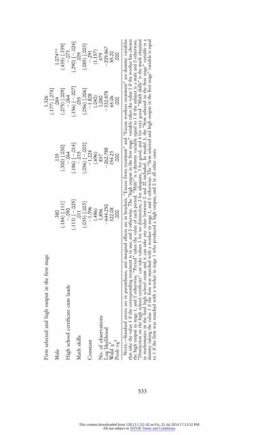
Table 4 presents a regression that highlights the determinants of whether
This content downloaded from 128.111.121.42 on Fri, 25 Jul 2014 17:13:52 PMAll use subject to JSTOR Terms and Conditions

Competition and the Ratchet Effect 535
a firm chooses the high rental fee in the second stage. We estimate random-effects Probit models on second-stage data pooled across treatments(model 1) and on each treatment separately (models 2–4), taking intoaccount the fact that firms make repeated decisions. In all models, exceptmodel 3 for the excess firms treatment, we only consider observationswhen the firm was matched with a worker in the first stage. In model 1,“excess firms treatment” and “excess workers treatment” are dummy var-iables that take the value 1 if the corresponding treatment is in use, and0 otherwise. The other explanatory variables include the worker’s choiceof “high output in the first stage” (the variable takes the value 1 if theworker has chosen the high output in stage 1, and 0 otherwise). We interactthis variable with each treatment in the first regression. In regression 3,we add a dummy for whether the firm was selected in the first stage andthe same variable is interacted with the choice of a high output by theworker (the “firm selected and high output in the first stage” dummyvariable) since we predict that being matched with an agent who haschosen high output in stage 1 should lead the firm to offer a high rentalfee in stage 2. We also include a time trend (the period number from 1to 20) and the same individual characteristics as in table 3 (namely, thegender, the distinction obtained on the final high school, and the markobtained in mathematics in this exam). The mean and standard deviationof each independent variable are given in table B1 in appendix B, availablein the online version of the Journal of Labor Economics.
The regressions show no significant time trend except in the excessfirms treatment.30 Firms’ behavior is mainly influenced by the structureof the labor market and by the worker’s behavior in the first stage. Incomparison to the baseline treatment, firms were substantially more likelyto offer a high-fee contract in the excess workers treatment and substan-tially less likely to do so in the excess firms treatment. This can be seenfrom model 1, indicating that the probability of choosing the high rentalfee increases by 46.4 percentage points in the excess workers treatmentcompared with the baseline (this is significant at the 1% level), while itdecreases by 14.7 percentage points in the excess firms treatment (signif-icant at the 5% level), all else equal. This shows that firms reacted strongly
30 In the excess firms treatment, the coefficient associated with the “period”variable is significant with a 99% confidence interval. This suggests that the in-dividuals’ decisions evolve over time, possibly because firms learn to cope withcompetition as they accumulate more experience in that treatment. As a robustnesstest, we have estimated the same models with robust standard errors and clusteringat the individual level. The only difference is that the time trend loses significancewhen data are pooled. In contrast, the excess firms treatment dummy gains sig-nificance at the 1% level, as well as the high output in first stage in excess workerstreatment in regression 1.
This content downloaded from 128.111.121.42 on Fri, 25 Jul 2014 17:13:52 PMAll use subject to JSTOR Terms and Conditions

536 Charness et al.
Table 5Workers’ Decisions to Switch Firms in the Second Stage,Excess Firms Treatment
Incumbent Firm’s Offer
Low Second-Stage Fee High Second-Stage Fee
Competitor’s Offer High Fee Low Fee Total High Fee Low Fee Total
Decision to switch 0 (0) 54 (42.86) 54 (42.86) 3 (5.56) 48 (88.88) 51 (94.44)Decision not to switch 12 (9.52) 60 (47.62) 72 (57.14) 3 (5.56) 0 (0) 3 (5.56)
Total 12 (9.52) 114 (90.48) 126 (100) 6 (11.12) 48 (88.88) 54 (100)
Note.—Percentages are in parentheses.
to the labor-market conditions, consistent with the qualitative theoreticalpredictions.
Overall, firms were more likely to choose the high-fee contract afterhaving observed a high output in the first stage, as the probability ofchoosing the high fee is increased by a remarkable 90.3 percentage pointsin this case (significant at the 1% level). This is consistent with the qual-itative predictions of the theoretical model when the firm can identify thetalent of his worker from his first-stage choice of output. In the excessfirms treatment, being selected in the first stage reduces the likelihood ofoffering a high fee in the second stage by 5.7 percentage points all elseequal (significant at the 1% level), but the worker choosing a high outputin stage one instead of a low output increases the likelihood by 21.7percentage points (same level of significance). This marginal effect of thechoice of a high output in stage 1 on the probability of offering a highfee in stage 2 is smaller than in the other treatments (it is 89.9 percentagepoints in the baseline and 51.2 in the excess workers treatment). This islikely due to the fact that when firms must compete with other firms tohire a worker, they are less likely to exploit the high talent of their worker(as revealed in the first stage) than in the other labor-market conditions,as predicted. Indeed, recall that the only PBNE in this treatment is aseparating equilibrium, in which workers choose type-appropriate out-puts in the first stage and incumbents do not take advantage of this in-formation in the second stage—they offer low second-stage fees to allworkers, regardless of the worker’s first-stage effort choices.
C. Switching Decisions
When there is competition on the market, the switching decisions arealso informative. Table 5 displays the workers’ decisions in the secondstage of the excess firms treatment depending on the second-stage feeschosen by the incumbent firm and its competitor.
This table shows that it never pays for a firm to choose the high rentalfee in the second stage since doing so leads the agent to select the con-tractual offer of the competitor. When both firms choose the high fee,
This content downloaded from 128.111.121.42 on Fri, 25 Jul 2014 17:13:52 PMAll use subject to JSTOR Terms and Conditions

Competition and the Ratchet Effect 537
Table 6Firms’ Decisions to Switch Workers in the Second Stage,Excess-Agents Treatment
Worker Chooses High Effortin Stage 1
Worker Chooses Low Effortin Stage 1
Second-StageFee High Fee Low Fee Total High Fee Low Fee Total
Decision toswitch
10 (6.90) 3 (2.07) 13 (8.97) 66 (19.76) 59 (17.66) 125 (37.43)
Decision not toswitch
126 (86.90) 6 (4.14) 132 (91.03) 88 (26.35) 121 (36.23) 209 (62.57)
Total 136 (93.79) 9 (6.21) 145 (100) 154 (46.11) 180 (53.89) 334 (100)
Note.—Percentages are in parentheses.
the workers are indifferent.31 In a random-effects Probit model analyzingthe workers’ probability of switching firms (not reported here but avail-able upon request), we find that being matched with two firms choosinga high fee reduces the likelihood that the worker switches firms by 41.83percentage points, while being matched with two firms choosing the lowfee reduces this likelihood by 32.70 percentage points.32
Similarly, table 6 reports descriptive statistics on the firms’ decisionsto switch agents between the first and the second stages in the excessworkers treatment. As indicated by table 6, nearly 87% of the firms whosefirst-stage worker selected high effort propose the high fee in the secondstage to the same worker. In a random-effects Probit model analyzing thefirms’ probability to switch workers (not reported here but available uponrequest), we find that being matched with a worker choosing a high outputin the first stage reduces the likelihood that the firm switches workers inthe second stage by 31.67 percentage points, a significant change.33 De-
31 Interestingly, we do not find clear evidence of inequity aversion. Indeed,inequity-averse workers would switch firms who make similar offers to reducethe difference of payoffs between the two firms across the period.
32 This regression is based on a random-effects Probit model in which theindependent variable is the worker’s decision to switch firms between stages 1and 2. The independent variables include two dummy variables indicating thatboth firms offer the high fee or the low fee, a time trend, and demographic variables(gender, cognitive abilities proxied by the distinction obtained on the final highschool exam and by the mark obtained in mathematics in this exam). The numberof observations is 180. The log-likelihood is �103.885. Only the two dummyvariables capturing the firms’ offers of the high fee or the low fee are significant( and , respectively).p p .049 p ! .001
33 This regression is based on a random-effects Probit model in which theindependent variable is the firm’s decision to switch worker between the twostages. The independent variables include the output of the worker in the firststage, a time trend, and demographic variables (gender, cognitive abilities proxiedby the distinction obtained on the final high school exam and by the mark obtainedin mathematics in this exam). The number of observations is 479. The log-like-lihood is �231.209. Only the output of the worker in the previous stage is sig-nificant.
This content downloaded from 128.111.121.42 on Fri, 25 Jul 2014 17:13:52 PMAll use subject to JSTOR Terms and Conditions

538 Charness et al.
cisions are more complex when the first-stage worker selects low effort,presumably because this reveals less information to firms. Still, in bothof the pure-strategy PBNE of the excess workers treatment, firms in thissituation should always make their first offer—a low fee—to the unem-ployed worker. In our experiment, however, only 37% of the firms inthis situation switched workers at the end of stage 1. This may be dueto naive play or to a reluctance to change workers. Also in contrast withthe two pure-strategy PBNE, 46% of firms in this situation offered thehigh fee at the start of stage 2. This should not happen in the pure-strategyPBNE but might be part of a mixed-strategy equilibrium to this game.
D. Earnings
Finally, we examine the total earnings of firms and workers in ourexperiment and assess their consistency with the theoretical predictionsof our model. According to the model, firms should earn more (andworkers less) when there is competition among workers than in the base-line treatment. This is confirmed by Mann-Whitney tests at the individuallevel, with for firms and for workers; at the sessionp p .002 p ! .001level, for both firms and workers. Similarly, firms should earnp p .050less (and workers more) in the excess firms treatment than in the baseline.For firms, this is also confirmed by Mann-Whitney tests at the individuallevel ( ; at the session level, ). For workers, it is confirmedp ! .001 p p .050at the individual level with and at the session level withp ! .001 p p
.34.050To summarize, viewed through the lens of our theoretical model, a
reasonable interpretation of the results from our two competitive treat-ments seems to be the following. The excess firms treatment improvesworkers’ outside options (by adding the possibility of trading with adifferent firm) while holding firms’ outside options fixed (at zero). Afterthis improvement, it is risky for firms to demand a high rental fee evenif the firm knows that the worker has high talent, since the worker mightchoose to work for another firm instead. As a result, most firms tend to
34 The model performs less well in predicting the actual levels of earnings. Forfirms, these are 51.21 ECU with excess workers, 47.11 in the baseline, and 22.62with excess firms. Comparing these with the predicted levels from app. A (57,45, and 22.5, respectively), two-sided t-tests with each individual as an observationindicate that actual earnings are significantly lower than predicted in the excessworkers treatment ( ), higher than predicted in the baseline ( ),p ! .001 p p .007and not different from the prediction in the excess firms treatment ( ).p p .830High-talent workers’ actual mean earnings are 103.80 with excess firms, 80.16 inthe baseline, and 43.66 with excess workers. Comparing these to the predictedlevels (105, 92.5, and 59.2, respectively), two-sided t-tests indicate that actualearnings are significantly lower than predicted in the excess firms treatment( ), the baseline ( ), and the excess workers treatment ( ).p p .004 p ! .001 p ! .001
This content downloaded from 128.111.121.42 on Fri, 25 Jul 2014 17:13:52 PMAll use subject to JSTOR Terms and Conditions

Competition and the Ratchet Effect 539
post low fees even when they observe high first-stage output (i.e., re-gardless of the worker’s first-stage behavior). Anticipating this, high-talentworkers are less motivated to undertake inefficient first-stage actions toconceal their identity.
The excess workers treatment, in contrast, improves firms’ outside op-tions (by adding the possibility of trading with a different worker) whileholding workers’ outside options fixed (at zero). Now firms can offer thehigh fee initially to either the employed or the unemployed worker ifthey observe high first-stage output, and a large majority does this. Moreimportantly, however, the fact that firms exercise their option to makeoffers to unemployed workers in equilibrium reduces high-talent workers’incentives to conceal their identity by picking low first-stage output. Putmore succinctly, competition among firms restricts firms’ ability to takeadvantage of private information if they have it, while competition amongworkers restricts the amount workers can hope to gain by concealingprivate information. In both cases, increased competition improves thetransmission of private information.
V. Conclusion
Since at least Akerlof’s (1970) classic article, it has been widely rec-ognized that asymmetric information can create market failures that arerobust to the presence of competition. Indeed, in some simple asymmetricinformation models (such as Akerlof’s “lemons” model), a reduction intrading frictions can cause markets to completely collapse, leading tosignificant welfare losses. In this paper, however, we provide an examplefrom the labor market where increased competition improves the per-formance of markets with asymmetric information: output restriction byworkers essentially disappears when we introduce ex post competitionfor either workers or jobs. While Kanemoto and MacLeod (1992) pre-dicted this in a more general model of competition between principals,to our knowledge no studies have predicted or tested this effect of expost competition between agents.
Intuitively, ratchet effects differ from other asymmetric-informationproblems in that information is concealed by one party in order to preventthe other party from exploiting its ex post monopoly power in a repeatedrelationship. Thus, one might expect that reductions in such ex post powertend to eliminate ratchet effects. In more detail, improving either party’sex post outside options reduces the total amount of quasi-rents availableto be divided between the agent and principal. This, in turn, reduces theeffect that information revelation can possibly have on the informedparty’s payoffs, thus reducing the payoffs to concealing that information.Notably, this process does not require the market (in our case, nonin-cumbent principals) to observe the same things (in particular, the previous
This content downloaded from 128.111.121.42 on Fri, 25 Jul 2014 17:13:52 PMAll use subject to JSTOR Terms and Conditions

540 Charness et al.
performance of the agent) that are seen by the contracting parties; thusit operates even when the outside “market” is at an informational dis-advantage relative to insiders. A second, important reason why ex postcompetition alleviates asymmetric-information problems is the fact thatit introduces the possibility of turnover. Simply put, the private returnto making (costly) investments in concealment is reduced if informedagents are less likely to interact with the thus-uninformed party in thefuture. While our model is highly specific, it seems likely that both ofthese principles carry over to much more general contexts.
Perhaps the above considerations help explain the increasing use ofincentive pay in the U.S. economy (see, e.g., Kuhn and Lozano 2008,table 11; or Lemieux, MacLeod and Parent 2009), as increasing interna-tional competition, falling mobility costs, deregulation, and deunioniza-tion have made U.S. labor markets more competitive. According to ourmodel and our laboratory evidence, such increased competition shouldreduce the scope for strategic output restriction by workers of the sortonce familiar in case studies of U.S. industry. Under the assumptions ofour model, this raises economic efficiency by mitigating the asymmetricinformation problem that gives rise to those restrictions.
Appendix A
Equilibrium in the Three Treatments
I. Baseline (No Competition) Case
In the second stage, high-talent workers accept both low (30) and high(66) fees, yielding a profit to the firm equal to the fee charged. Low-talentworkers accept only the low fee, yielding a profit of 30 if the low fee ischarged and zero if the high fee is charged. Thus, the firm’s expectedprofits if it charges the high fee are , where p is the66p � 0(1 � p) p 66pfirm’s subjective probability that the worker is high talent. The firm’sprofits from charging the low fee are 30, independent of its beliefs becauseboth worker types accept this offer. Thus, the firm will post the high feeat the start of stage 2 if and only if (iff) 66 , or .p 1 30 p 1 5/11
Now suppose a separating equilibrium in pure strategies in which bothworkers choose type-appropriate first-stage outputs, thus revealing theirtypes. Firms who observe a high first-stage output will therefore set
and charge a high second-stage fee. Thus, in equilibrium, a high-p p 1ability worker’s payoff will be 35 in the first stage and 34 in the secondstage for a total of 69. A high-productivity worker who deviates fromthis equilibrium by choosing low output in the first stage receives
. Thus, there can be no such separating equilibrium.22.5 � 70 p 92.5In a pooling equilibrium, both worker types select low output in stage
1; thus at the start of stage 2. The firm therefore sets a low feep p 1/3
This content downloaded from 128.111.121.42 on Fri, 25 Jul 2014 17:13:52 PMAll use subject to JSTOR Terms and Conditions

Competition and the Ratchet Effect 541
in the second stage. Equilibrium payoffs are for the22.5 � 70 p 92.5high-talent workers. Now consider the expected payoffs of a high-pro-ductivity worker who deviates from this equilibrium by selecting highoutput in the first stage. Since low-talent workers always choose loweffort, firms should infer that any worker deviating to high effort is ofhigh talent and will impose a high second-stage fee if such deviations areobserved, leading to a payoff of . Thus, it does not pay a35 � 34 p 69high-talent worker to deviate from this pooling equilibrium. It also doesnot pay for the firm to deviate by charging a high fee in the second stageafter observing low output, since in our design. Therefore,p p 1/3 ! 5/11a pure pooling equilibrium does exist.
In sum, in the baseline (no competition) case, there is only one purestrategy equilibrium. It is a pooling equilibrium in which both workertypes select low effort in the first stage. Firms learn nothing from workers’first-stage behavior and offer low fees to both worker types in stage 2.These offers are always accepted. Firms’ predicted payoffs are therefore15 and 30 in stages 1 and 2, for a total of 45. Talented workers’ predictedpayoffs, as already noted, are .22.5 � 70 p 92.5
II. Excess Firms Case
In this case two firms (the “incumbent” and “outsider”) play a simul-taneous fee-offer game to an agent of (potentially) uncertain type in thesecond stage. Depending on the worker’s output history at the incumbentfirm, the firms might have different priors concerning the worker’s type.Assuming that workers choose at random between identical offers, thepayoff matrix confronting these two firms is given in the table below,where p and q respectively are the incumbent and outsider firms’ beliefs(at the start of the second stage) that the worker is high talent.
Outside Firm’s Offer
Low Fee High Fee
Incumbent’sPayoff
Outsider’sPayoff
Incumbent’sPayoff
Outsider’sPayoff
Incumbent firm’s offer:Low fee 15 15 30 0High fee 0 30 33p 33q
These values are derived as follows: If both firms choose the low fee(30), this is accepted regardless of the worker’s type. In this case (andwhenever workers or firms face identical offers henceforth), we assumethat the worker will choose at random from the two identical offers foran expected payoff of 15. If the two firms choose different offers, eithertype of worker will choose the low offer; thus the firm charging the highfee gets a payoff of zero, and the other firm’s offer is accepted with
This content downloaded from 128.111.121.42 on Fri, 25 Jul 2014 17:13:52 PMAll use subject to JSTOR Terms and Conditions

542 Charness et al.
certainty for a payoff of 30. If both firms charge a high fee, the incumbentfirm’s expected payoff is 66 (the high fee) times its assessment of theprobability the worker is of high talent (p), times 0.5 (the chance that theworker picks the incumbent). The outside firm’s payoff in this situationis calculated in the same manner.
Examination of this table reveals that the low fee is a strictly dominantstrategy for the outside firm iff . Next, note that the outsideq ! 10/11firm does not observe the worker’s first-stage effort decision. (It does, ofcourse, observe which firm the worker chose to work for in the first stage,but this choice reveals no information about the worker since both firmsoffer the low fee in the first stage.) Thus we must have , and theq p 1/3outside firm will always offer a low fee. Given this, then according tothe above payoff table the incumbent will always choose a low fee aswell; in other words given Bayesian beliefs for the outside firm, the onlyNash equilibrium to this simultaneous-offer second-stage subgame is forboth firms to offer a low fee, regardless of the incumbent firm’s beliefs.(Even if it is certain its worker has high talent, the incumbent firm willnot demand a high fee because it should rationally anticipate that itscompetitor will offer a low fee.)
Finally, since workers of both types know they will receive low-fee offersfrom both firms in the second stage regardless of workers’ first-stage actions,workers’ first-stage actions will simply maximize their first-stage utilities.The only PBNE in the excess firms case is thus a separating equilibrium,in which workers choose type-appropriate outputs in the first stage; in-cumbents correctly infer the workers’ types in the second stage but do nottake advantage of this information—they offer low second-stage fees to allworkers, regardless of the worker’s first-stage effort choices.35 The expectedpayoff of firms is just , since all firms make low fee offers in15 � 30 p 45both periods, and these offers are always accepted by both worker types.High-ability workers face low fees and choose high effort in both periods,so their equilibrium payoffs are .35 � 70 p 105
35 This result, like Kanemoto and MacLeod’s, is robust to the introduction ofsmall worker mobility costs. To see this, imagine that, when faced with identicaloffers, workers choose the incumbent firm’s offer with probability . Thenr 1 0.5for all , the outside firm’s strictly dominant strategy is still to set ther � [0.5, 1)low fee for all . Since q must still equal 1/3 for outside firms, outsideq ! 10/11firms must offer the low fee in any equilibrium. Given this, the incumbent firmcan expect 30r if it sets the low fee and zero if it sets the high fee. Thus, onceagain the only equilibrium has firms making low-fee offers to all workers in thesecond stage, regardless of their first-stage actions. Collusion between firms toimpose the high fee when facing a high-talent worker is very unlikely due to theinformation structure of the game.
This content downloaded from 128.111.121.42 on Fri, 25 Jul 2014 17:13:52 PMAll use subject to JSTOR Terms and Conditions

Competition and the Ratchet Effect 543
III. Excess Workers Case
In this treatment, firms must offer the same fee to the employed andunemployed workers, but may make the offers in any order. Thus, a firmnow must choose among four second-stage actions, offering the high orlow fee to either the employed or unemployed worker. (Any offers thatare turned down are then offered to the other worker.)
Low fees are always accepted by the first worker to get them; thus thefirm’s payoff when it offers the low fee to either worker first is just 30(the low fee). When the firm offers the high fee, then regardless of theorder of the offers, the firm receives a payoff of zero if neither the em-ployed or unemployed worker is able, and 66 otherwise. The probabilityneither worker is able is Pr (U low talentFE low talent) # Pr (E low
. Thus the firm will offer the high fee ifftalent) p (11/17) # (1 � p), or . As with the low fee,(11/17) # (1 � p) # 66 1 30 p 1 36/121 ≈ .296
the firm is indifferent to which worker receives the offer first; this is trueregardless of its prior, p.
Given these facts, we can now check for the existence of certain kindsof equilibria.
A. Can a Pure Separating Equilibrium Exist?
By definition, in a pure separating equilibrium, all high-talent workerschoose high first-stage output and all low-talent workers choose low first-stage output, and therefore firms set when they see high first-stagep p 1output and when they see low first-stage output. It thus followsp p 0from the above facts that, in any pure separating equilibrium, firms willoffer a high fee in the second stage whenever the employed worker’s first-stage output was high, and a low second-stage fee to both workers whenthe employed worker’s first-stage output was low.
We need to consider four different types of pure separating equilibrium.
Case 1. Firms initially make their second-stage offer to the employedworker, regardless of the employed worker’s first-stage outputchoice. In this proposed separating equilibrium, an able workergets . If he deviates by picking low first-stage35 � 34 p 69output, he gets , so he will deviate. So this22.5 � 70 p 92.5separating equilibrium does not survive.
Case 2. Firms initially make their second-stage offer to the unemployedworker, regardless of the employed worker’s first stage effortchoice. In this proposed separating equilibrium, an able incum-bent worker gets (the firm chooses the35 � (12/17) # 34 p 59high fee, having observed high output in stage 1). If he deviatesby picking low first-stage output (in which case the firmchooses a low fee in stage 2, since the firm believes that theemployed worker is less able and ) he gets(6/17) # 66 ! 30
This content downloaded from 128.111.121.42 on Fri, 25 Jul 2014 17:13:52 PMAll use subject to JSTOR Terms and Conditions
544 Charness et al.
, so there is no profitable deviation. This is a22.5 � 0 p 22.5PBNE.
Case 3. Firms initially make their second-stage offer to the employedworker if the employed worker’s first-stage output choice ishigh, and to the unemployed worker if the employed worker’sfirst-stage output is low. In this proposed separating equilib-rium, an able incumbent worker gets . If he de-35 � 34 p 69viates by picking low first-stage output, he gets 22.5 � 0 p
, so there is no profitable deviation. This is a PBNE.22.5Case 4. Firms initially make their second-stage offer to the unemployed
worker if the employed worker’s first-stage output choice ishigh, and to the employed worker if the employed worker’sfirst-stage output choice is low. In this proposed separatingequilibrium, an able worker gets . If35 � (12/17) # 34 p 59he deviates by picking low first-stage output, he gets 22.5 �
, so he will definitely deviate. So this separating equi-70 p 92.5librium does not survive.
Putting all these cases together, there are two pure-strategy, separatingPBNE. In both, firms make high second-stage fee offers when they seehigh first-stage output and low second-stage offers otherwise, and in-cumbent workers who choose low first-stage effort are reemployed bythe firm with probability strictly less than one.36
B. Can a Pure Pooling Equilibrium Exist?
Recall that we force all our low-talent workers to always choose loweffort, so pooling can only occur at the low level of first-stage output.Further, if all workers choose low first-stage output, firm’s second-stageprior, p, will equal 1/3 for all workers, both employed and unemployed.Therefore, firms will always prefer the high second-stage fee, since thelikelihood that at least one of the workers will accept the offer is 1 �
, and .(2/3) # (11/17) p 29/51 (29/51) # 66 1 30We now consider an able worker’s incentives to deviate from these
proposed pooling equilibria. (Low-talent workers cannot deviate, by con-struction, and wouldn’t want to anyway because choosing high output
36 If we allow firms to randomize over which worker receives the second-stageoffer first, additional equilibria with these same two features also emerge. Forexample, consider just the class of equilibria in which the “routing” of the firm’ssecond-stage offer is not conditional on the observed first-stage output, and let abe the probability that the firm makes its first offer to the employed worker. Then,combining cases 1 and 2, the able incumbent gets in35 � 34a � (12/17)34(1 � a)the separating equilibrium. He gets if he deviates. It follows that there22.5 � 70ais also a continuum of PBNE in which the employed worker unconditionallyreceives the first offer with probability .a ! 73/120
This content downloaded from 128.111.121.42 on Fri, 25 Jul 2014 17:13:52 PMAll use subject to JSTOR Terms and Conditions
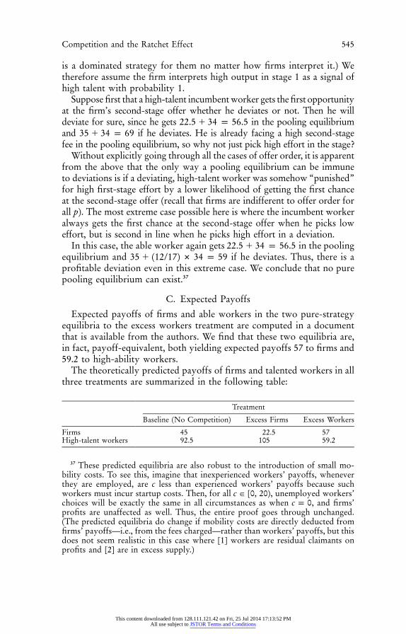
Competition and the Ratchet Effect 545
is a dominated strategy for them no matter how firms interpret it.) Wetherefore assume the firm interprets high output in stage 1 as a signal ofhigh talent with probability 1.
Suppose first that a high-talent incumbent worker gets the first opportunityat the firm’s second-stage offer whether he deviates or not. Then he willdeviate for sure, since he gets in the pooling equilibrium22.5 � 34 p 56.5and if he deviates. He is already facing a high second-stage35 � 34 p 69fee in the pooling equilibrium, so why not just pick high effort in the stage?
Without explicitly going through all the cases of offer order, it is apparentfrom the above that the only way a pooling equilibrium can be immuneto deviations is if a deviating, high-talent worker was somehow “punished”for high first-stage effort by a lower likelihood of getting the first chanceat the second-stage offer (recall that firms are indifferent to offer order forall p). The most extreme case possible here is where the incumbent workeralways gets the first chance at the second-stage offer when he picks loweffort, but is second in line when he picks high effort in a deviation.
In this case, the able worker again gets in the pooling22.5 � 34 p 56.5equilibrium and if he deviates. Thus, there is a35 � (12/17) # 34 p 59profitable deviation even in this extreme case. We conclude that no purepooling equilibrium can exist.37
C. Expected Payoffs
Expected payoffs of firms and able workers in the two pure-strategyequilibria to the excess workers treatment are computed in a documentthat is available from the authors. We find that these two equilibria are,in fact, payoff-equivalent, both yielding expected payoffs 57 to firms and59.2 to high-ability workers.
The theoretically predicted payoffs of firms and talented workers in allthree treatments are summarized in the following table:
Treatment
Baseline (No Competition) Excess Firms Excess Workers
Firms 45 22.5 57High-talent workers 92.5 105 59.2
37 These predicted equilibria are also robust to the introduction of small mo-bility costs. To see this, imagine that inexperienced workers’ payoffs, wheneverthey are employed, are c less than experienced workers’ payoffs because suchworkers must incur startup costs. Then, for all , unemployed workers’c � [0, 20)choices will be exactly the same in all circumstances as when , and firms’c p 0profits are unaffected as well. Thus, the entire proof goes through unchanged.(The predicted equilibria do change if mobility costs are directly deducted fromfirms’ payoffs—i.e., from the fees charged—rather than workers’ payoffs, but thisdoes not seem realistic in this case where [1] workers are residual claimants onprofits and [2] are in excess supply.)
This content downloaded from 128.111.121.42 on Fri, 25 Jul 2014 17:13:52 PMAll use subject to JSTOR Terms and Conditions

546 Charness et al.
References
Akerlof, George A. 1970. The market for “lemons”: Quality uncertaintyand the market mechanism. Quarterly Journal of Economics 84, no. 3(August): 488–500.
Allen, Douglas W., and Dean Lueck. 1999. Searching for ratchet effectsin agricultural contracts. Journal of Agricultural and Resource Econom-ics 24, no. 2 (December): 536–52.
Brandts, Jordi, and Gary Charness. 2004. Do labour market conditionsaffect gift exchange? Some experimental evidence. Economic Journal114 (July): 684–708.
Cabrales, Antonio, Gary Charness, and Marie Claire Villeval. Forthcom-ing. Competition, hidden information and efficiency: An experiment.Experimental Economics.
Carmichael, H. Lorne, and W. Bentley MacLeod. 2000. Worker coop-eration and the ratchet effect. Journal of Labor Economics 18, no. 1(January): 1–19.
Chaudhuri, Ananish. 1998. The ratchet principle in a principal agent gamewith unknown costs: An experimental analysis. Journal of EconomicBehavior and Organization 37, no. 3 (November): 291–304.
Choi, Jay-Pil, and Marcel Thum. 2003. The dynamics of corruption withthe ratchet effect. Journal of Public Economics 87, nos. 3–4 (March):427–43.
Cooper, David J., John H. Kagel, Wei Lo, and Qing Liang Gu. 1999.Gaming against managers in incentive systems: Experimental resultswith Chinese students and Chinese managers. American Economic Re-view 89, no. 4 (September): 781–804.
Dalen, Dag-Morten. 1995. Efficiency-improving investment and theratchet effect. European Economic Review 39, no. 8 (October): 1511–22.
Dearden, James, Barry W. Ickes, and Larry Samuelson. 1990. To innovateor not to innovate: Incentives and innovation in hierarchies. AmericanEconomic Review 80, no. 5 (December): 1105–24.
Dewatripont, Mathias, Ian Jewitt, and Jean Tirole. 1999. The economicsof career concerns, part 1: Comparing information structure. Reviewof Economic Studies 66, no. 1 (January): 183–98.
Dillen, Mats, and Michael Lundholm. 1996. Dynamic income taxation,redistribution, and the ratchet effect. Journal of Public Economics 59,no. 1 (January): 69–93.
Farrell, Joseph, and Carl Shapiro. 1989. Optimal contracts with lock-in.American Economic Review 79, no. 1 (March): 51–68.
Freixas, Xavier, Roger Guesnerie, and Jean Tirole. 1985. Planning underincomplete information and the ratchet effect. Review of EconomicStudies 52, no. 2 (April): 173–91.
This content downloaded from 128.111.121.42 on Fri, 25 Jul 2014 17:13:52 PMAll use subject to JSTOR Terms and Conditions
Competition and the Ratchet Effect 547
Gibbons, Robert. 1987. Piece-rate incentive schemes. Journal of LaborEconomics 5 (October): 413–29.
Greiner, B. 2004. An online recruitment system for economic experiments.In Forschung und wissenschaftliches Rechnen 2003, ed. K. Kremer andV. Macho, 79–93. GWDG Bericht 63. Gottingen: Ges. fur Wiss. Da-tenverarbeitung.
Ickes, Barry W., and Larry Samuelson. 1987. Job transfers and incentivesin complex organizations: Thwarting the ratchet effect. RAND Journalof Economics 18, no. 2 (Summer): 275–86.
Kanemoto, Yoshitsugu, and W. Bentley MacLeod. 1992. The ratchet effectand the market for secondhand workers. Journal of Labor Economics10, no. 1 (January): 85–98.
Kuhn, Peter, and Fernando Lozano. 2008. The expanding workweek?Understanding trends in long work hours among U.S. men, 1979–2006.Journal of Labor Economics 26, no. 2 (April): 311–43.
Laffont, Jean-Jacques, and Jean Tirole. 1988. The dynamics of incentivecontracts. Econometrica 56:1153–75.
———. 1993. A theory of incentives in procurement and regulation. Cam-bridge, MA: MIT Press.
Lazear, Edward. 1998. Personnel economics for managers. New York:Wiley.
———. 2000. “Performance pay and productivity.” American EconomicReview 90, no. 3 (December): 1346–61.
Lemieux, Thomas, W. Bentley MacLeod, and Daniel Parent. 2009. Per-formance pay and wage inequality. Quarterly Journal of Economics 124,no. 1 (February): 1–49.
Litwack, John M. 1993. Coordination, incentives, and the ratchet effect.Rand Journal of Economics 24, no. 2 (Summer): 271–85.
Mathewson, Stanley B. 1931. Restriction of output among unorganizedworkers. New York: Viking Press.
Puller, Steven L. 2006. The strategic use of innovation to influence reg-ulatory standards. Journal of Environmental Economics and Manage-ment 52, no. 3 (November): 690–706.
Roland, Gerard, and Khalid Sekkat. 2000. Managerial career concerns,privatization and restructuring in transition economies. European Eco-nomic Review 44, no. 10 (December): 1857–72.
Weitzman, Martin L. 1980. The “ratchet principle” and performance in-centives. Bell Journal of Economics 11, no. 1 (Spring): 302–8.
This content downloaded from 128.111.121.42 on Fri, 25 Jul 2014 17:13:52 PMAll use subject to JSTOR Terms and Conditions