Nonparametric Bootstrap Procedures for PredictiveInference Based on Recursive Estimation Schemes1

Valentina Corradi∗ and Norman R. Swanson∗∗

∗Queen Mary, University of London and ∗∗Rutgers University

October 2005

Abstract

We introduce block bootstrap techniques that are (first order) valid in recursive estimation frameworks. There-

after, we present two examples where predictive accuracy tests are made operational using our new bootstrap proce-

dures. In one application, we outline a consistent test for out-of-sample nonlinear Granger causality, and in the other

we outline a test for selecting amongst multiple alternative forecasting models, all of which are possibly misspecified.

In a Monte Carlo investigation, we compare the finite sample properties of our block bootstrap procedures with the

parametric bootstrap due to Kilian (1999); within the context of encompassing and predictive accuracy tests. In the

empirical illustration, it is found that unemployment has nonlinear marginal predictive content for inflation.

JEL classification: C22, C51.

Running Title: Bootstrap for Predictive Inference

Keywords: block bootstrap, recursive estimation scheme, reality check, nonlinear causality, para-

meter estimation error.

1Valentina Corradi, Department of Economics, Queen Mary, University of London, Mile End Road, London E1

4NS, UK, v.corradi@qmul.ac.uk. Norman R. Swanson, Department of Economics, Rutgers University, 75 Hamilton

Street, New Brunswick, NJ 08901, USA, nswanson@econ.rutgers.edu. We owe a great many thanks to the editor,

Frank Schorfheide, and two referees for numerous useful suggestions, all of which we feel were instrumental in im-

proving earlier versions of this paper. Additionally, we wish to thank Jean-Marie Dufour, Silvia Goncalves, Stephen

Gordon, Clive Granger, Oliver Linton, Brendan McCabe, Antonio Mele, Andrew Patton, Rodney Strachan, Chris-

tian Schluter, Allan Timmerman, and seminar participants at Cornell University, the London School of Economics,

Laval University, Queen Mary, University of London, CIREQ-Universite’ de Montreal, the University of Liverpool,

Southampton University, the University of Virginia, the 2004 Winter Meetings of the Econometric Society, and the

Bank of Canada for useful comments and suggestions. Corradi gratefully acknowledges financial support via ESRC

grant RES-000-23-0006, and Swanson thanks the Rutgers University Research Council for financial support.

1 Introduction

Economic models are often compared in terms of their relative predictive accuracy. Thus, it is not

surprising that a large literature on the topic has developed over the last 10 years, including, for

example, important papers by Diebold and Mariano (DM: 1995), West (1996), and White (2000). In

this literature, it is quite common to compare multiple models (which are possibly all misspecified,

in the sense that they are all approximations of some unknown true model) in terms of their in- or

out-of-sample predictive accuracy, for a given loss function. In such contexts, one often compares

parametric models containing estimated parameters. Hence, it is important to take into account the

contribution of parameter estimation error when carrying out inference. Though some authors make

a case in favor of using in-sample predictive evaluation (important contributions in this area include

Inoue and Kilian (2004, 2005)), it is common practice to split samples of size T into T = R + P

observations, where only the last P observations are used for predictive evaluation, particularly if

all models are assumed to be (possibly) misspecified. We consider such a setup, and assume that

parameters are estimated in recursive fashion, such that R observations are used to construct a

first parameter estimator, say θR, a first prediction (say a 1-step ahead prediction), and a first

prediction error. Then, R + 1 observations are used to construct θR+1, yielding a second ex ante

prediction and prediction error. This procedure is continued until a final estimator is constructed

using T−1 observations, resulting in a sequence of P = T−R estimators, predictions, and prediction

errors. If R and P grow at the same rate as the sample size, the limiting distributions of predictive

accuracy tests using this setup generally reflects the contribution of parameter uncertainty (i.e. the

contribution of 1√P

∑T−1t=R

(θt − θ†

), where θt is a recursive m−estimator constructed using the first

t observations, and θ† is its probability limit, say).2 Given this fact, our objectives in this paper

are twofold. First, we introduce block bootstrap techniques that are (first order) valid in recursive

estimation frameworks. Thereafter, we present two examples where predictive accuracy tests are

made operational using our new bootstrap procedures. One of the examples involves constructing a

consistent test for out-of-sample nonlinear Granger causality, and the other involves constructing a

test for selecting amongst multiple alternative forecasting models, all of which may be misspecified.

In some circumstances, such as when constructing Diebold and Mariano (1995) tests for equal

(pointwise) predictive accuracy of two models, the limiting distribution is a normal random vari-

able. In such cases, accounting for the contribution of parameter estimation error can be often2m−estimators include least squares, nonlinear least square, (quasi) maximum likelihood, and exactly identified

instrumental variables and generalized method of moments estimators.

1

done using the framework of West (1996), and essentially involves estimating an “extra” covariance

term. However, in other circumstances, such as when constructing tests which have power against

generic alternatives, test statistics have limiting distributions that can be shown to be functionals

of Gaussian processes with covariance kernels that reflect both (dynamic) misspecification as well

as the contribution of (recursive) parameter estimation error. Such limiting distributions are not

nuisance parameter free, and critical values cannot be tabulated. However, valid asymptotic critical

values can be obtained via appropriate application of the (block) bootstrap. This requires a boot-

strap procedure that allows for the formulation of statistics which properly mimic the contribution

of 1√P

∑T−1t=R

(θt − θ†

)(i.e. parameter estimation error). The first objective of this paper is thus

to suggest a block bootstrap procedure which is valid for recursive m-estimators, in the sense that

its use suffices to mimic the limiting distribution of 1√P

∑T−1t=R

(θt − θ†

).

When forming the block bootstrap for recursivem-estimators, it is important to note that earlier

observations are used more frequently than temporally subsequent observations when forming test

statistics. On the other hand, in the standard block bootstrap, all blocks from the original sample

have the same probability of being selected, regardless of the dates of the observations in the blocks.

Thus, the bootstrap estimator, say θ∗t , which is constructed as a direct analog of θt, is characterized

by a location bias that can be either positive or negative, depending on the sample that we observe.

In order to circumvent this problem, we suggest a re-centering of the bootstrap score which ensures

that the new bootstrap estimator, which is no longer the direct analog of θt, is asymptotically

unbiased. It should be noted that the idea of re-centering is not new in the bootstrap literature for

the case of full sample estimation. In fact, re-centering is necessary, even for first order validity,

in the case of overidentified generalized method of moments (GMM) estimators (see e.g. Hall and

Horowitz (1996), Andrews (2002, 2004), and Inoue and Shintani (2004)). This is due to the fact

that, in the overidentified case, the bootstrap moment conditions are not equal to zero, even if

the population moment conditions are. However, in the context of m−estimators using the full

sample, re-centering is needed only for higher order asymptotics, but not for first order validity,

in the sense that the bias term is of smaller order than T−1/2 (see e.g. Andrews (2002)). In the

case of recursive m−estimators, on the other hand, the bias term is instead of order T−1/2, so that

it does contribute to the limiting distribution. This points to a need for re-centering when using

recursive estimation schemes, and such re-centering is discussed in the next section.

The block bootstrap for recursive m-estimators that we develop can be used to provide valid

critical values in a variety of interesting testing contexts, two such leading examples of which are

2

developed in this paper. As mentioned above, the first is a generalization of the reality check

test of White (2000) that allows for non vanishing parameter estimation error. The second is an

out-of-sample version of the integrated conditional moment (ICM) test of Bierens (1982,1990) and

Bierens and Ploberger (1997), which yields out-of-sample tests that are consistent against generic

(nonlinear) alternatives.3 More specifically, our first application concerns the reality check of White

(2000), which itself extends the Diebold and Mariano (1995) and West (1996) test for the relative

predictive accuracy of two models by allowing for the joint comparison of multiple misspecified

models against a given benchmark. The idea of White (2000) is to compare all competing models

simultaneously, thus taking into account any correlation across the various models. In this context,

the null hypothesis is that no competing model can outperform the benchmark, for a given loss

function. As this test is usually carried out by comparing predictions from various alternative

models, and given that predictions are usually formed using recursively estimated models, the issue

of parameter estimation uncertainty arises naturally. White (2000) obtains valid asymptotic critical

values for his test via use of the Politis and Romano (1994) stationary bootstrap for the case in

which parameter estimation error is asymptotically negligible. This is the case in which either the

same loss function is used for both estimation and model evaluation, or P grows at a slower rate

than R. Using the block bootstrap for recursive m-estimators, we generalize the reality check to

the case in which parameter estimation error does not vanish asymptotically.

The objective of the second application is to test the predictive accuracy of a given (non)linear

model against generic (non)linear alternatives. In particular, one chooses a benchmark model, and

the objective is to test whether there is an alternative model which can provide more accurate,

loss function specific, out-of-sample predictions. The test is based on a continuum of moment

conditions and is consistent against generic alternatives, as discussed in Corradi and Swanson (CS:

2002). The CS test differs from the ICM test developed by Bierens (1982,1990) and Bierens and

Ploberger (1997) because parameters are estimated recursively, out-of-sample prediction models are

analyzed, and the null hypothesis is that the reference model delivers the best “loss function specific”

predictor, for a given information set. Given that the test compares out-of-sample prediction

models, it can be viewed as a test for (non)linear out-of-sample Granger causality. Although

the CS test examined in this application is the same as that discussed in Corradi and Swanson

(2002), it should be noted that they use a conditional p-value method for constructing critical

values, extending earlier work by Hansen (1996) and Inoue (2001). However, the conditional p-3An application to predictive density and confidence interval forecast evaluation is given in Corradi and Swanson

(2005).

3

value approach suffers from the fact that under the alternative, the simulated statistics diverges at

rate√l, conditional on the sample, where l plays a role analogous to the block length in the block

bootstrap. This feature clearly leads to reduced power in finite samples, as shown in Corradi and

Swanson (2002). As an alternative to the conditional p-value approach, we establish in our second

example that the bootstrap for recursive m−estimators yields√P -consistent CS tests.

In order to shed evidence on the usefulness of the recursive block bootstrap, we carry out

a Monte Carlo investigation that compares the finite sample properties of our block bootstrap

procedures with two alternative naive block bootstraps as well as the parametric bootstrap due

to Kilian (1999); all within the context of the CS test and a simpler non-generic version of the

CS test due to Chao, Corradi and Swanson (CCS: 2001). In addition, various other related tests,

including the standard F-test as well as tests due to Diebold and Mariano (1995) and Clark and

McCracken (2004) are included in our Monte Carlo experiments. Results suggest that our recursive

block bootstrap outperforms alternative naive nonparametric block bootstraps. Additionally, the

Kilian bootstrap is shown to be robust to nonlinear misspecification, and all of the test statistics

examined are found to have good finite sample properties when applied in situations where there

is model misspecification.

An empirical illustration is also discussed, in which it is found that unemployment appears to

have nonlinear marginal predictive content for inflation, as evidenced by application of the CS and

CCS test. Findings based upon the other tests mentioned above are also presented, and it turns

out that much can be learned by using all of the 5 tests in consort with one another. Namely, the

different tests have different power properties against different alternatives, and hence the use of

several of them can yield insight into the nature of the misspecification driving test rejection. In

particular, the picture that emerges when only a subset of the tests is used to analyze the marginal

predictive content of unemployment for inflation is that of an absence of predictive ability. When

all of the tests are used, on the other hand, interesting evidence arises concerning the potential

nonlinear predictive content of unemployment. Thus, the tests discussed in this illustration appear

to be useful complements to each other.

The rest of the paper is organized as follows. Section 2 outlines the block bootstrap for recur-

sive m−estimators and contains asymptotic results. Sections 3 and 4 contain the two examples

mentioned above. Monte Carlo findings are discussed in Section 5, and our empirical illustration is

presented in Section 6. Finally, concluding remarks are given in Section 7. All proofs are collected

in an appendix. Hereafter, P ∗ denotes the probability law governing the resampled series, condi-

4

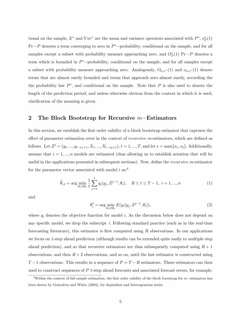
tional on the sample, E∗ and V ar∗ are the mean and variance operators associated with P ∗, o∗P (1)

Pr−P denotes a term converging to zero in P ∗−probability, conditional on the sample, and for all

samples except a subset with probability measure approaching zero, and O∗P (1) Pr−P denotes a

term which is bounded in P ∗−probability, conditional on the sample, and for all samples except

a subset with probability measure approaching zero. Analogously, Oa.s.∗(1) and oa.s.∗(1) denote

terms that are almost surely bounded and terms that approach zero almost surely, according the

the probability law P ∗, and conditional on the sample. Note that P is also used to denote the

length of the prediction period, and unless otherwise obvious from the context in which it is used,

clarification of the meaning is given.

2 The Block Bootstrap for Recursive m−Estimators

In this section, we establish the first order validity of a block bootstrap estimator that captures the

effect of parameter estimation error in the context of recursive m-estimators, which are defined as

follows. Let Zt = (yt, ..., yt−s1+1, Xt, ..., Xt−s2+1), t = 1, ..., T, and let s = max{s1, s2}. Additionally,

assume that i = 1, ..., n models are estimated (thus allowing us to establish notation that will be

useful in the applications presented in subsequent sections). Now, define the recursive m-estimator

for the parameter vector associated with model i as:4

θi,t = arg minθi∈Θi

1t

t∑j=s

qi(yj , Zj−1, θi), R ≤ t ≤ T − 1, i = 1, ..., n (1)

and

θ†i = arg minθi∈Θi

E(qi(yj , Zj−1, θi)), (2)

where qi denotes the objective function for model i. As the discussion below does not depend on

any specific model, we drop the subscript i. Following standard practice (such as in the real-time

forecasting literature), this estimator is first computed using R observations. In our applications

we focus on 1-step ahead prediction (although results can be extended quite easily to multiple step

ahead prediction), and so that recursive estimators are thus subsequently computed using R + 1

observations, and then R+ 2 observations, and so on, until the last estimator is constructed using

T − 1 observations. This results in a sequence of P = T −R estimators. These estimators can then

used to construct sequences of P 1-step ahead forecasts and associated forecast errors, for example.4Within the context of full sample estimation, the first order validity of the block bootstrap for m−estimators has

been shown by Goncalves and White (2004), for dependent and heterogeneous series.

5

Now, consider the overlapping block resampling scheme of Kunsch (1989), which can be applied

in our context as follows:5 At each replication, draw b blocks (with replacement) of length l from the

sample Wt = (yt, Zt−1), where bl = T − s. Thus, the first block is equal to Wi+1, ...,Wi+l, for some

i = s−1, ..., T − l+1, with probability 1/(T −s− l+1), the second block is equal to Wi+1, ...,Wi+l,

again for some i = s−1, ..., T−l+1, with probability 1/(T−s−l+1), and so on, for all blocks, where

the block length grows with the sample size at an appropriate rate. More formally, let Ik, k = 1, ..., b

be iid discrete uniform random variables on [s−1, s, ..., T − l+1]. Then, the resampled series, W ∗t =

(y∗t , Z∗,t−1), is such that W ∗

1 ,W∗2 , ...,W

∗l ,W

∗l+1, ...,W

∗T = WI1+1,WI1+2, ...,WI1+l,WI2+1, ...,WIb+l,

and so a resampled series consists of b blocks that are discrete iid uniform random variables,

conditional on the sample.

Suppose we define the bootstrap estimator, θ∗t , to be the direct analog of θt. Namely,

θ∗t = arg minθ∈Θ

1t

t∑j=s

q(y∗j , Z∗,j−1, θ), R ≤ t ≤ T − 1. (3)

By first order conditions, 1t

∑tj=s∇θq(y∗j , Z

∗,j−1, θ∗t ) = 0, and via a mean value expansion of1t

∑tj=s∇θq(y∗j , Z

∗,j−1, θ∗t ) around θt, after a few simple manipulations, we have that

1√P

T−1∑t=R

(θ∗t − θt

)

=1√P

T−1∑t=R

−1t

t∑j=s

∇2θq(y

∗j , Z

∗,j−1, θ∗t )

−1

1t

t∑j=s

∇θq(y∗j , Z∗,j−1, θt)

= B† 1√

P

T−1∑t=R

1t

t∑j=s

∇θq(y∗j , Z∗,j−1, θt)

+ oP ∗(1) Pr−P

= B†aR,0√P

R∑j=s

∇θq(y∗j , Z∗,j−1, θR) +B† 1√

P

P−1∑j=1

aR,j∇θq(y∗R+j , Z∗,R+j−1, θR+j)

+oP ∗(1) Pr−P, (4)5The main difference between the block bootstrap and the stationary bootstrap of Politis and Romano (PR:1994)

is that the former uses a deterministic block length, which may be either overlapping as in Kunsch (1989) or non-

overlapping as in Carlstein (1986), while the latter resamples using blocks of random length. One important feature

of the PR bootstrap is that the resampled series, conditional on the sample, is stationary, while a series resampled

from the (overlapping or non overlapping) block bootstrap is nonstationary, even if the original sample is strictly

stationary. However, Lahiri (1999) shows that all block boostrap methods, regardless of whether the block length is

deterministic or random, have a first order bias of the same magnitude, but the bootstrap with deterministic block

length has a smaller first order variance. In addition, the overlapping block boostrap is more efficient than the non

overlapping block bootstrap.

6

where θ∗t ∈(θ∗t , θt

), B† = E

(−∇2

θq(yj , Zj−1, θ†)

)−1, aR,j = 1

R+j + 1R+j+1 + ... + 1

R+P−1 , j =

0, 1, ..., P − 1, and where the last equality on the right hand side of (4) follows immediately, using

the same arguments as those used in Lemma A5 of West (1996). Analogously,

1√P

T−1∑t=R

(θt − θ†

)= B†aR,0√

P

R∑j=s

∇θq(yj , Zj−1, θ†) +B† 1√

P

P−1∑j=1

aR,j∇θq(yR+j , ZR+j−1, θ†) + oP (1). (5)

Now, given (2), E(∇θq(yj , Z

j−1, θ†))

= 0 for all j, and 1√P

∑T−1t=R

(θt − θ†

)has a zero mean

normal limiting distribution (see Theorem 4.1 in West (1996)). On the other hand, as any block of

observations has the same chance of being drawn,

E∗(∇θq(y∗j , Z

∗,j−1, θt))

=1

T − s

T−1∑k=s

∇θq(yk, Zk−1, θt) +O

(l

T

)Pr−P, (6)

where the O(

lT

)term arises because the first and last l observations have a lesser chance of be-

ing drawn (see e.g. Fitzenberger (1997)).6 Now, 1T−s

∑T−1k=s ∇θq(yk, Z

k−1, θt) 6= 0, and is instead

of order OP

(T−1/2

). Thus, 1√

P

∑T−1t=R

1T−s

∑T−1k=s ∇θq(yk, Z

k−1, θt) = OP (1), and does not vanish in

probability. This clearly contrasts with the full sample case, in which 1T−s

∑T−1k=s ∇θq(yk, Z

k−1, θT ) =

0, because of the first order conditions. Thus, 1√P

∑T−1t=R

(θ∗t − θt

)cannot have a zero mean normal

limiting distribution, but is instead characterized by a location bias that can be either positive or

negative depending on the sample.

Given (6), our objective is thus to have the bootstrap score centered around 1T−s

∑T−1k=s ∇θq(yk, Z

k−1, θt).

Hence, define a new bootstrap estimator, θ∗t , as:

θ∗t = arg minθ∈Θ

1t

t∑j=s

(q(y∗j , Z

∗,j−1, θ)− θ′

(1T

T−1∑k=s

∇θq(yk, Zk−1, θt)

)), (7)

R ≤ t ≤ T − 1.7

Now, note that first order conditions are 1t

∑tj=s

(∇θq(y∗j , Z

∗,j−1, θ∗t )−(

1T

∑T−1k=s ∇θq(yk, Z

k−1, θt)))

=

0; and via a mean value expansion of 1t

∑tj=s∇θq(y∗j , Z

∗,j−1, θ∗t ) around θt, after a few simple ma-

6In fact, the first and last observation in the sample can appear only at the beginning and end of the block, for

example.7More precisely, we should use 1

t−sand 1

T−sto scale the summand in (7). For notational simplicity, 1

t−sand 1

T−s

are approximated with 1t

and 1T

.

7

nipulations, we have that:

1√P

T−1∑t=R

(θ∗t − θt

)

= B† 1√P

T∑t=R

1t

t∑j=s

(∇θq(y∗j , Z

∗,j−1, θt)−

(1T

T−1∑k=s

∇θq(yk, Zk−1, θt)

))+oP ∗(1), Pr−P.

Thus, given (6), it is immediate to see that the bias associated with 1√P

∑T−1t=R

(θ∗t − θt

)is of

order O(lT−1/2

), conditional on the sample, and so it is negligible for first order asymptotics, as

l = o(T 1/2).

Theorem 1, which summarizes these results, requires the following assumptions.

Assumption A1: (yt, Xt), with yt scalar and Xt an <ζ−valued (0 < ζ <∞) vector, is a strictly

stationary and absolutely regular β−mixing process with size −4(4 + ψ)/ψ, ψ > 0.

Assumption A2: (i) θ† is uniquely identified (i.e. E(q(yt, Zt−1, θ)) > E(q(yt, Z

t−1, θ†)) for any

θ 6= θ†); (ii) q is twice continuously differentiable on the interior of Θ, and for Θ a compact subset

of <%; (iii) the elements of ∇θq and ∇2θq are p−dominated on Θ, with p > 2(2 + ψ), where ψ is

the same positive constant as defined in Assumption A1; and (iv) E(−∇2

θq(θ))

is negative definite

uniformly on Θ.8

Assumption A3: T = R+ P, and as T →∞, P/R→ π, with 0 < π <∞.

Assumptions A1 and A2 are standard memory, moment, smoothness and identifiability condi-

tions. A1 requires (yt, Xt) to be strictly stationary and absolutely regular. The memory condition

is stronger than α−mixing, but weaker than (uniform) φ−mixing. Assumption A3 requires that

R and P grow at the same rate. In fact, if P grows at a slower rate than R, i.e. P/R → 0, then1√P

∑Tt=R

(θt − θ†

)= oP (1) and so there were no need to capture the contribution of parameter

estimation error.

Theorem 1: Let A1-A3 hold. Also, assume that as T →∞, l→∞, and that lT 1/4 → 0. Then, as

T, P and R→∞,

P

(ω : sup

v∈<%

∣∣∣∣∣P ∗T(

1√P

T∑t=R

(θ∗t − θt

)≤ v

)− P

(1√P

T∑t=R

(θt − θ†

)≤ v

)∣∣∣∣∣ > ε

)→ 0,

where P ∗T denotes the probability law of the resampled series, conditional on the (entire) sample.

8We say that ∇θq(yt, Zt−1, θ) is 2r−dominated on Θ if its j − th element, j = 1, ..., %, is such that

��∇θq(yt, Z

t−1, θ)��j≤ Dt, and E(|Dt|2r) < ∞. For more details on domination conditions, see Gallant and White

(1988, pp. 33).

8

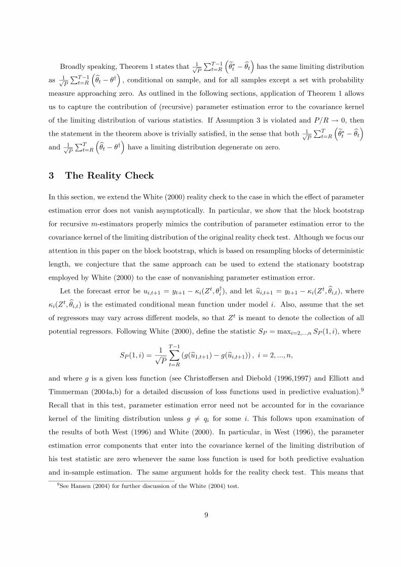
Broadly speaking, Theorem 1 states that 1√P

∑T−1t=R

(θ∗t − θt

)has the same limiting distribution

as 1√P

∑T−1t=R

(θt − θ†

), conditional on sample, and for all samples except a set with probability

measure approaching zero. As outlined in the following sections, application of Theorem 1 allows

us to capture the contribution of (recursive) parameter estimation error to the covariance kernel

of the limiting distribution of various statistics. If Assumption 3 is violated and P/R → 0, then

the statement in the theorem above is trivially satisfied, in the sense that both 1√P

∑Tt=R

(θ∗t − θt

)and 1√

P

∑Tt=R

(θt − θ†

)have a limiting distribution degenerate on zero.

3 The Reality Check

In this section, we extend the White (2000) reality check to the case in which the effect of parameter

estimation error does not vanish asymptotically. In particular, we show that the block bootstrap

for recursive m-estimators properly mimics the contribution of parameter estimation error to the

covariance kernel of the limiting distribution of the original reality check test. Although we focus our

attention in this paper on the block bootstrap, which is based on resampling blocks of deterministic

length, we conjecture that the same approach can be used to extend the stationary bootstrap

employed by White (2000) to the case of nonvanishing parameter estimation error.

Let the forecast error be ui,t+1 = yt+1 − κi(Zt, θ†i ), and let ui,t+1 = yt+1 − κi(Zt, θi,t), where

κi(Zt, θi,t) is the estimated conditional mean function under model i. Also, assume that the set

of regressors may vary across different models, so that Zt is meant to denote the collection of all

potential regressors. Following White (2000), define the statistic SP = maxi=2,...,n SP (1, i), where

SP (1, i) =1√P

T−1∑t=R

(g(u1,t+1)− g(ui,t+1)) , i = 2, ..., n,

and where g is a given loss function (see Christoffersen and Diebold (1996,1997) and Elliott and

Timmerman (2004a,b) for a detailed discussion of loss functions used in predictive evaluation).9

Recall that in this test, parameter estimation error need not be accounted for in the covariance

kernel of the limiting distribution unless g 6= qi for some i. This follows upon examination of

the results of both West (1996) and White (2000). In particular, in West (1996), the parameter

estimation error components that enter into the covariance kernel of the limiting distribution of

his test statistic are zero whenever the same loss function is used for both predictive evaluation

and in-sample estimation. The same argument holds for the reality check test. This means that9See Hansen (2004) for further discussion of the White (2004) test.

9

as long as g = qi ∀i, the White test can be applied regardless of the rate of growth of P and

R. When we write the covariance kernel of the limiting distribution of the statistic (see below),

however, we include terms capturing the contribution of parameter estimation error, thus implicitly

assuming that g 6= qi for some i. In practice, one reason why we allow for cases where g 6= qi is that

least squares is sometimes better behaved in finite samples and/or easier to implement than more

generic m−estimators, so that practitioners sometimes use least squares for estimation and more

complicated (possibly asymmetric) loss functions for predictive evaluation.10 Of course, there are

also applications for which parameter estimation error does not vanish, even if the same loss function

is used for parameter estimation and predictive evaluation. One such application is discussed in

the next section.

For a given loss function, the reality check tests the null hypothesis that a benchmark model

(defined as model 1) performs equal to or better than all competitor models (i.e. models 2,...,n).

The alternative is that at least one competitor performs better than the benchmark.11 Formally,

the hypotheses are:

H0 : maxi=2,...,n

E (g(u1,t+1)− g(ui,t+1)) ≤ 0

and

HA : maxi=2,...,n

E (g(u1,t+1)− g(ui,t+1)) > 0.

In order to derive the limiting distribution of SP we require the following additional assumption.

Assumption A4: (i) κi is twice continuously differentiable on the interior of Θi and the elements

of ∇θiκi(Zt, θi) and ∇2

θiκi(Zt, θi) are p−dominated on Θi, for i = 2, ..., n, with p > 2(2+ψ), where

ψ is the same positive constant as that defined in Assumption A1; (ii) g is positive valued, twice

continuously differentiable on Θi, and g, g′ and g′′ are p−dominated on Θi with p defined as in (i);

and (iii) let Sgigi = limT→∞ V ar(

1√T

∑Tt=s (g(u1,t+1)− g(ui,t+1))

), i = 2, ..., n, define analogous

covariance terms, Sgjgk, j, k = 2, ..., n, and assume that [Sgjgk

] is positive semi-definite.

Assumptions A4(i)-(ii) are standard smoothness and domination conditions imposed on the

conditional mean functions of the models. Assumption A4(iii) is standard in the literature that10Consider linex loss, where g(u) = eau − au − 1, so that for a > 0 (a < 0) positive (negative) errors are more

(less) costly than negative (positive) errors. Here, the errors are exponentiated, so that in this particular case, laws

of large numbers and central limit theorems may require a large number of observations before providing satisfactory

approximations. This feature of linex loss is illustrated in the Monte Carlo findings of Corradi and Swanson (2002).

(Linex loss is studied in Zellner (1986), Christoffersen and Diebold (1996, 1997) and Granger (1999), for example.)11In the current context, we are interested in choosing the model which is more accurate for given loss function. An

alternative approach is to combine different forecasting models in some optimal way. For very recent contributions

along these lines, see Elliott and Timmermann (2004a,b).

10

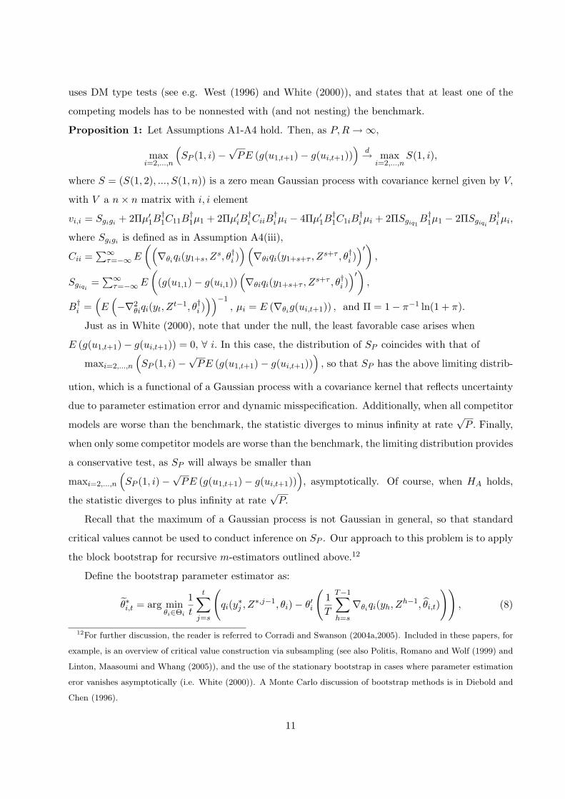
uses DM type tests (see e.g. West (1996) and White (2000)), and states that at least one of the

competing models has to be nonnested with (and not nesting) the benchmark.

Proposition 1: Let Assumptions A1-A4 hold. Then, as P,R→∞,

maxi=2,...,n

(SP (1, i)−

√PE (g(u1,t+1)− g(ui,t+1))

)d→ max

i=2,...,nS(1, i),

where S = (S(1, 2), ..., S(1, n)) is a zero mean Gaussian process with covariance kernel given by V,

with V a n× n matrix with i, i element

vi,i = Sgigi + 2Πµ′1B†1C11B

†1µ1 + 2Πµ′iB

†iCiiB

†iµi − 4Πµ′1B

†1C1iB

†iµi + 2ΠSgiq1

B†1µ1 − 2ΠSgiqi

B†iµi,

where Sgigi is defined as in Assumption A4(iii),

Cii =∑∞

τ=−∞E

((∇θi

qi(y1+s, Zs, θ†i )

)(∇θiqi(y1+s+τ , Z

s+τ , θ†i ))′)

,

Sgiqi=∑∞

τ=−∞E

((g(u1,1)− g(ui,1))

(∇θiqi(y1+s+τ , Z

s+τ , θ†i ))′)

,

B†i =

(E(−∇2

θiqi(yt, Zt−1, θ†i )

))−1, µi = E (∇θi

g(ui,t+1)) , and Π = 1− π−1 ln(1 + π).

Just as in White (2000), note that under the null, the least favorable case arises when

E (g(u1,t+1)− g(ui,t+1)) = 0, ∀ i. In this case, the distribution of SP coincides with that of

maxi=2,...,n

(SP (1, i)−

√PE (g(u1,t+1)− g(ui,t+1))

), so that SP has the above limiting distrib-

ution, which is a functional of a Gaussian process with a covariance kernel that reflects uncertainty

due to parameter estimation error and dynamic misspecification. Additionally, when all competitor

models are worse than the benchmark, the statistic diverges to minus infinity at rate√P . Finally,

when only some competitor models are worse than the benchmark, the limiting distribution provides

a conservative test, as SP will always be smaller than

maxi=2,...,n

(SP (1, i)−

√PE (g(u1,t+1)− g(ui,t+1))

), asymptotically. Of course, when HA holds,

the statistic diverges to plus infinity at rate√P.

Recall that the maximum of a Gaussian process is not Gaussian in general, so that standard

critical values cannot be used to conduct inference on SP . Our approach to this problem is to apply

the block bootstrap for recursive m-estimators outlined above.12

Define the bootstrap parameter estimator as:

θ∗i,t = arg minθi∈Θi

1t

t∑j=s

(qi(y∗j , Z

∗,j−1, θi)− θ′i

(1T

T−1∑h=s

∇θiqi(yh, Z

h−1, θi,t)

)), (8)

12For further discussion, the reader is referred to Corradi and Swanson (2004a,2005). Included in these papers, for

example, is an overview of critical value construction via subsampling (see also Politis, Romano and Wolf (1999) and

Linton, Maasoumi and Whang (2005)), and the use of the stationary bootstrap in cases where parameter estimation

eror vanishes asymptotically (i.e. White (2000)). A Monte Carlo discussion of bootstrap methods is in Diebold and

Chen (1996).

11

where R ≤ t ≤ T−1, i = 1, ..., n. Further, define the bootstrap statistic as S∗P = maxi=2,...,n S∗P (1, i),

where:

S∗P (1, i) =1√P

T−1∑t=R

[(g(y∗t+1 − κ1(Z∗,t, θ∗1,t))− g(y∗t+1 − κi(Z∗,t, θ∗i,t))

)

−

1T

T−1∑j=s

(g(yj+1 − κ1(Zj , θ1,t))− g(yj+1 − κi(Zj , θi,t))

) . (9)

Note that bootstrap statistic in (9) is different from the “usual” bootstrap statistic, which is defined

as the difference between the statistic computed over the sample observations and over the bootstrap

observations. That is, following the usual approach to bootstrap statistic construction, one might

have expected that the appropriate bootstrap statistic would be:

S∗P (1, i) =

1√P

T−1∑t=R

[(g(y∗t+1 − κ1(Z∗,t, θ∗1,t))− g(y∗t+1 − κi(Z∗,t, θ∗i,t))

)−(g(yt+1 − κ1(Zt, θ1,t))− g(yt+1 − κi(Zt, θi,t))

)]. (10)

Instead, as can be seen by inspection of S∗P (1, i), the bootstrap (resampled) component is con-

structed only over the last P observations, while the sample component is constructed over all

T observations. Although a formal proof is provided in the appendix, it is worthwhile to give a

heuristic explanation of the validity of the statistic in (9). For sake of simplicity, consider a single

model, say model 1. Now,

1√P

T−1∑t=R

g(y∗t+1 − κ1(Z∗,t, θ∗1,t))−1T

T−1∑j=s

g(yj+1 − κ1(Zj , θ1,t))

=

1√P

T−1∑t=R

g(y∗t+1 − κ1(Z∗,t, θ1,t))−1T

T−1∑j=s

g(yj+1 − κ1(Zj , θ1,t))

+

1√P

T−1∑t=R

∇θg(y∗t+1 − κ1(Z∗,t, θ∗1,t))

(θ∗1,t − θ1,t

), (11)

where θ∗1,t ∈(θ∗1,t, θ1,t

). Notice that the first term on the RHS of (11) mimics the limiting behav-

ior of 1√P

∑T−1t=R (g(u1,t+1)− E(g(u1,t+1))) , while the second term mimics the limiting behavior of

the parameter estimation error associated with model 1. Needless to say, the same holds for any

arbitrary model. This leads to the following theorem.

Theorem 2: Let Assumptions A1-A4 hold. Also, assume that as T → ∞, l → ∞, and thatl

T 1/4 → 0. Then, as T, P and R→∞,

P

(ω : sup

v∈<

∣∣∣∣P ∗T ( maxi=2,...,n

S∗P (1, i) ≤ v

)− P

(max

i=2,...nSµ

P (1, i) ≤ v

)∣∣∣∣ > ε

)→ 0,

12

and

SµP (1, i) = SP (1, i)−

√PE (g(u1,t+1)− g(ui,t+1)) ,

The above result suggests proceeding in the following manner. For any bootstrap replication,

compute the bootstrap statistic, S∗P . Perform B bootstrap replications (B large) and compute the

quantiles of the empirical distribution of the B bootstrap statistics. Reject H0, if SP is greater

than the (1 − α)th-percentile. Otherwise, do not reject. Now, for all samples except a set with

probability measure approaching zero, SP has the same limiting distribution as the corresponding

bootstrapped statistic when E (g(u1,t+1)− g(ui,t+1)) = 0 ∀ i, ensuring asymptotic size equal to α.

On the other hand, when one or more competitor models are strictly dominated by the benchmark,

the rule provides a test with asymptotic size between 0 and α (see above discussion). Under the

alternative, SP diverges to (plus) infinity, while the corresponding bootstrap statistic has a well

defined limiting distribution, ensuring unit asymptotic power.

4 The CS Test

CS (2002) draw on both the consistent specification and predictive ability testing literatures in order

to propose a test for predictive accuracy which is consistent against generic nonlinear alternatives,

which is designed for comparing nested models, and which allows for dynamic misspecification of

all models being evaluated. The CS test is an out-of-sample version of the ICM test, as discussed

in the introduction of this paper. This test is relevant for model selection, as it is well known that

DM and reality check tests do not have a well defined limiting distributions when the benchmark is

nested with all competing models and when P/R→ 0 (see e.g. Corradi and Swanson (2002, 2004b),

McCracken (2004) and Clark and McCracken (2004)).13 Alternative (non DM) tests for comparing

the predictive ability of a fixed number of nested models have previously also been suggested.

For example, Clark and McCracken (2001,2004) propose encompassing tests for comparing two

nested models for one-step and multi-step ahead prediction, respectively. Giacomini and White

(2003) introduce a test for conditional predictive ability that is valid for both nested and nonnested

models. The key ingredient of their test is the fact that parameters are estimated using a fixed13McCracken (2004) provides a very interesting result based on a version of the DM test in which loss is quadratic

and martingale difference scores are assumed (i.e. it is assumed that the model is correctly specified under the null

hypothesis). In particular, he shows that in this case, the DM test has a nonstandard limiting distribution which is

a functional of Brownian motions, whenever P/R → π > 0. Clark and McCracken (2004) extend McCracken (2004)

to the case of multi step ahead forecasts.

13

rolling window. Finally, Inoue and Rossi (2004) suggest a recursive test, where not only the

parameters, but the statistic itself, are computed in a recursive manner.

The main difference between these tests and the CS test is that the CS test is consistent against

generic (non)linear alternatives and not only against a fixed alternative.

Summarizing the testing approach considered in this application, assume that the objective is

to test whether there exists any unknown alternative model that has better predictive accuracy

than a given benchmark model, for a given loss function. A typical example is the case in which the

benchmark model is a simple autoregressive model and we want to check whether a more accurate

forecasting model can be constructed by including possibly unknown (non)linear functions of the

past of the process or of the past of some other process (e.g. out-of-sample (non)linear Granger

causality tests can be constructed in this manner).14 Although this is the case that we focus

on, the benchmark model can in general be any (non)linear model. One important feature of

this application is that the same loss function is used for in-sample estimation and out-of-sample

prediction (see Granger (1993), Weiss (1996), and Schorfheide (2005) for further discussion of this

issue)15. In contrast to the previous application, however, this does not ensure that parameter

estimation error vanishes asymptotically.

Let the benchmark model be:

yt = θ†1,1 + θ†1,2yt−1 + u1,t, (12)

where θ†1 = (θ†1,1, θ†1,2)

′ = arg minθ1∈Θ1 E(q1(yt−θ1,1−θ1,2yt−1)), θ1 = (θ1,1, θ1,2)′, yt is a scalar, and

q1 = g, as the same loss function is used both for in-sample estimation and out-of-sample predictive

evaluation. The generic alternative model is:

yt = θ†2,1(γ) + θ†2,2(γ)yt−1 + θ†2,3(γ)w(Zt−1, γ) + u2,t(γ), (13)

where θ†2(γ) = (θ†2,1(γ), θ†2,2(γ), θ

†2,3(γ))

′ = arg minθ2∈Θ2 E(q1(yt − θ2,1 − θ2,2yt−1 − θ2,3w(Zt−1, γ))),

θ2(γ) = (θ2,1(γ), θ2,2(γ), θ2,3(γ))′, θ2 ∈ Θ2, Γ is a compact subset of <d, for some finite d. The

alternative model is called “generic” because of the presence of w(Zt−1, γ), which is a generi-

cally comprehensive function, such as Bierens’ exponential, a logistic, or a cumulative distribution14For example, Swanson and White (1997) compare the predictive accuracy of various linear models against neural

network models using both in-sample and out-of-sample model selection criteria.15In the context of multi-step ahead vector autoregressive prediction, Schorfheide (2005) proposes a new prediction

criterion that can be used to jointly select the number of lags as well as to choose between (quasi)-maximum likelihood

estimators and loss function based estimators.

14

function (see e.g. Stinchcombe and White (1998) for a detailed explanation of generic comprehen-

siveness). One example has w(Zt−1, γ) = exp(∑s2

i=1 γiΦ(Xt−i)), where Φ is a measurable one to

one mapping from < to a bounded subset of <, so that here Zt = (Xt, ..., Xt−s2+1), and we are

thus testing for nonlinear Granger causality. The hypotheses of interest are:

H0 : E(g(u1,t+1)− g(u2,t+1(γ))) = 0 versus HA : E(g(u1,t+1)− g(u2,t+1(γ))) > 0. (14)

Clearly, the reference model is nested within the alternative model, and given the definitions of θ†1

and θ†2(γ), the null model can never outperform the alternative.16 For this reason, H0 corresponds

to equal predictive accuracy, while HA corresponds to the case where the alternative model out-

performs the reference model, as long as the errors above are loss function specific forecast errors.

It follows that H0 and HA can be restated as:

H0 : θ†2,3(γ) = 0 versus HA : θ†2,3(γ) 6= 0,

for ∀γ ∈ Γ, except for a subset with zero Lebesgue measure. Now, given the definition of θ†2(γ),

note that

E

g′(yt+1 − θ†2,1(γ)− θ†2,2(γ)yt − θ†2,3(γ)w(Zt, γ))×

−1

−yt

−w(Zt, γ)

= 0,

where g′ is the derivative of the loss function with respect to its argument. Thus, under H0 we

have that θ†2,3(γ) = 0, θ†2,1(γ) = θ†1,1, θ†2,2(γ) = θ†1,2, and E(g′(u1,t+1)w(Zt, γ)) = 0. Thus, we can

once again restate H0 and HA as:

H0 : E(g′(u1,t+1)w(Zt, γ)) = 0 versus HA : E(g′(u1,t+1)w(Zt, γ)) 6= 0, (15)

for ∀γ ∈ Γ, except for a subset with zero Lebesgue measure. Finally, define the forecast error as

u1,t+1 = yt+1 −(

1 yt

)θ1,t. Following CS, the test statistic is:

MP =∫

ΓmP (γ)2φ(γ)dγ, (16)

where

mP (γ) =1

P 1/2

T−1∑t=R

g′(u1,t+1)w(Zt, γ), (17)

16Needless to say, in finite samples the forecasting mean square prediction error from the small model can be lower

than that associated with the larger model. Indeed, this property arises in our empirical illustration.

15

and where∫Γ φ(γ)dγ = 1, φ(γ) ≥ 0, with φ(γ) absolutely continuous with respect to Lebesgue

measure. Note also that “ ′ ” denotes derivative with respect to the argument of the function.

Elsewhere, we use “∇x” to denote derivative with respect to x. In the sequel, we require the

following assumptions.

Assumption A5: (i) w is a bounded, twice continuously differentiable function on the interior of

Γ and ∇γw(Zt, γ) is bounded uniformly in Γ; and (ii) ∇γ∇θ1q′1,t(θ1)w(Zt−1, γ) is continuous on

Θ1 × Γ, where q′1,t(θ1) = q′1(yt − θ1,1 − θ1,2yt−1), Γ a compact subset of <d, and is 2r−dominated

uniformly in Θ1 × Γ, with r ≥ 2(2 + ψ), where ψ is the same positive constant as that defined in

Assumption A1.

Assumption A5 requires the function w to be bounded and twice continuously differentiable;

such a requirement is satisfied by logistic or exponential functions, for example.

Proposition 2: Let Assumptions A1-A3 and A5 hold. Then, the following results hold: (i) Under

H0,

MP =∫

ΓmP (γ)2φ(γ)dγ d→

∫ΓZ(γ)2φ(γ)dγ,

where mP (γ) is defined in equation (17) and Z is a Gaussian process with covariance kernel given

by:

K(γ1, γ2) = Sgg(γ1, γ2) + 2Πµ′γ1B†ShhB

†µγ2 + Πµ′γ1B†Sgh(γ2)

+Πµ′γ2B†Sgh(γ1),

with µγ1 = E(∇θ1(g′t+1(u1,t+1)w(Zt, γ1))), B† = (E(∇2

θ1q1(u1,t)))−1,

Sgg(γ1, γ2) =∑∞

j=−∞E(g′(u1,s+1)w(Zs, γ1)g′(u1,s+j+1)w(Zs+j , γ2)),

Shh =∑∞

j=−∞E(∇θ1q1(u1,s)∇θ1q1(u1,s+j)′),

Sgh(γ1) =∑∞

j=−∞E(g′(u1,s+1)w(Zs, γ1)∇θ1q1(u1,s+j)′), and γ, γ1, and γ2 are generic elements of

Γ.

(ii) Under HA, for ε > 0, limP→∞ Pr(

1P

∫ΓmP (γ)2φ(γ)dγ > ε

)= 1.

As in the previous application, the limiting distribution under H0 is a Gaussian process with a

covariance kernel that reflects both the dependence structure of the data and the effect of parameter

estimation error. Hence, critical values are data dependent and cannot be tabulated.

In order to implement this statistic using the block bootstrap for recursive m-estimators, de-

16

fine:17

θ∗1,t = (θ∗1,1,t, θ∗1,2,t)

′ = arg minθ1∈Θ1

1t

t∑j=2

[q1(y∗j − θ1,1 − θ1,2y∗j−1)

−θ′11T

T−1∑i=2

∇θq1(yi − θ1,1,t − θ1,2,tyi−1)] (18)

Also, define u∗1,t+1 = y∗t+1 −(

1 y∗t

)θ∗1,t. The bootstrap test statistic is:

M∗P =

∫Γm∗

P (γ)2φ(γ)dγ,

where, recalling that g = q1,

m∗P (γ) =

1P 1/2

T−1∑t=R

(g′(y∗t+1 −

(1 y∗t

)θ∗1,t

)w(Z∗,t, γ)− 1

T

T−1∑i=2

g′(yi −

(1 yi−1

)θ1,t

)w(Zi−1, γ)

)(19)

As in the reality check case, the bootstrap statistic in (19) is characterized by the fact that

the bootstrap (resampled) component is constructed only over the last P observations, while the

sample component is constructed over all T observations. The same heuristic arguments given to

justify this form of bootstrap statistic in the previous application also apply here.

Theorem 3: Let Assumptions A1-A3 and A5 hold. Also, assume that as T → ∞, l → ∞, and

that lT 1/4 → 0. Then, as T, P and R→∞,

P

(ω : sup

v∈<

∣∣∣∣P ∗T (∫Γm∗

P (γ)2φ(γ)dγ ≤ v

)− P

(∫Γmµ

P (γ)2φ(γ)dγ ≤ v

)∣∣∣∣ > ε

)→ 0,

where mµP (γ) = mP (γ)−

√PE

(g′(u1,t+1)w(Zt, γ)

).

The above result suggests proceeding the same way as in the first application.

5 Monte Carlo Results

In this section we carry out a series of Monte Carlo experiments comparing the recursive block

bootstrap with a variety of other bootstraps, and comparing the finite sample performance of the

test discussed above with a variety of other tests. With regard to the bootstrap, we consider

4 alternatives. Namely: (i) the “Recur Block Bootstrap”, which is the block bootstrap for re-

cursive m-estimators discussed above; (ii) “Block Bootstrap, no PEE, no adjust” is a strawman

block bootstrap used for comparison purposes, where it is assumed that there is no parameter17Recall that y∗t , Z∗,t is obtained via the resampling procedure described in Section 2

17

estimation error (PEE), so that θ1,t is used in place of θ∗1,t in the construction of M∗P , and the term

1T

∑T−1i=1 g′

(yi+1 −

(1 yi

)θ1,t

)w(Zi, γ) inm∗

P is replaced with g′(yt+1 −

(1 yt

)θ1,t

)w(Zt, γ)

(i.e. there is no bootstrap statistic adjustment, thus conforming with the usual case when the stan-

dard block bootstrap is used); (iii) “Standard Block Bootstrap” is the standard block bootstrap

(i.e. this bootstrap is the same as that outlined in (ii), except that θ1,t is replaced with θ∗1,t; and

(iv) the parametric bootstrap of Kilian (1999), applied in the spirit of McCracken and Sapp (MS:

2005). As in MS, application of the parametric bootstrap begins with the estimation of a VAR

model for xt and yt (with lags selected using the Schwarz Information Criterion (SIC)) and re-

sample the residuals as if they were iid. Then the pseudo time series x∗t and y∗t are constructed

using estimated parameters and resampled residuals, and using the original VAR structure. At

this point, x∗t and y∗t are used to estimate parameters recursively and construct a series of one-step

ahead prediction errors (see below). Finally, bootstrap statistics are constructed exactly as are the

original statistics, except that prediction errors and variables are replaced with their bootstrapped

counterparts. It should be pointed out that a necessary condition for the asymptotic validity of

the Kilian (1999) parametric bootstrap is that the underlying DGP is nested by the VAR used in

the bootstrap procedure. Thus, it is not in general valid if the underlying DGP contains nonlinear

component(s).18 Furthermore, in our context, validity of this bootstrap still remains to be estab-

lished even in the case for which the DGP is nested by the linear VAR model. This is because the

bootstrap statistics are formed using one-step ahead forecast errors based on recursively estimated

parameters. Therefore, standard arguments used to show the validity of the parametric bootstrap

no longer apply. Nevertheless, it is interesting that the parametric bootstrap clearly still performs

quite well in a variety of nonlinear contexts, as shown in the experiments reported on below.

The test statistics examined in our experiments include: (i) the standard in-sample F-test;

(ii) the encompassing test due to Clark and McCracken (CM: 2004) and Harvey, Leybourne and

Newbold (1997); (iii) the Diebold and Mariano (DM: 1995) test; (iv) the CS test; and (v) the CCS

test.19

18See Kilian and Taylor (2003) for a modification of this procedure in the context of specific nonlinear models.

Additionally, note that even when the alternative is nonlinear, the parametric bootstrap of Kilian (1999) will have

correct size asymptotically, as long as the underlying model is linear under the null. In practice, one would expect

this bootstrap procedure to have power against some nonlinear alternatives, although it is not designed to have power

against general nonlinear alternatives.19The CCS statistic is essentially the same as the CS test, but uses Zt instead of a generically comprehensive

function thereof (recall that Zt contains the additional variables included in the “bigger” model defined below).

Thus, this test can be seen as a special case of the CS test that is designed to have power against linear alternatives,

18

To be more specific, note that the CM test is an out-of-sample encompassing test, and is defined

as follows:

CM = (P − h+ 1)1/21

P−h+1

∑T−ht=R ct+h

1P−h+1

∑j

j=−j

∑T−ht=R+j K

(jM

)(ct+h − c) (ct+h−j − c)

,

where ct+h = u1,t+h (u1,t+h − u2,t+h) , c = 1P−h+1

∑T−τt=R ct+h, K (·) is a kernel (such as the Bartlett

kernel), and 0 ≤ K(

jM

)≤ 1, with K(0) = 1, and M = o(P 1/2). Additionally, h is the forecast

horizon (set equal to unity in our experiments), P is as defined above, and u1,t+1 and u2,t+1 are the

out–of sample forecast errors associated with least squares estimation of “smaller” and “bigger”

linear models, respectively (see below for further details). Note that j does not grow with the

sample size. Therefore, the denominator in CM is a consistent estimator of the long run variance

only when E(ctct+|k|

)= 0 for all |k| > h (see Assumption A3 in Clark and McCracken (2004)).

Thus, the statistic takes into account the moving average structure of the multistep prediction

errors, but still does not allow for dynamic misspecification under the null. This is one of the main

differences between the CM and CS (CCS) tests.

Note also that the DM test is the mean square error version of the Diebold and Mariano (1995)

test for predictive accuracy, and is defined as follows:

DM =√P

1P

∑Tt=R dt+h

1P−h+1

∑j

j=−j

∑T−ht=R+j K

(jM

)(dt+h − d

)(dt+h−j − d

) ,where dt+h = u2

1,t+h− u22,t+h, and d = 1

P−h+1

∑T−τt=R dt+h. The limiting distributions of the CM and

DM statistics are given in Theorems 3.1 and 3.2 in Clark and McCracken (2004), and for h > 1

contain nuisance parameters so that critical values cannot be directly tabulated, and hence Clark

and McCracken (2004) use the Kilian parametric bootstrap to obtain critical values. In this case,

as discussed above, it is not clear that the parametric bootstrap is asymptotically valid. However,

again as alluded to above, the parametric bootstrap approach taken by Clark and McCracken is

clearly a good approximation, at least for the DGPs and horizon considered in our experiments,

given that these tests have very good finite sample properties (see discussion of results below).

and it is not explicitely designed to have power against generic nonlinear alternatives as is the CS test. The theory in

Section 4 of this paper thus applies to both the CS and CCS tests. Additionally, the CM test is included in our study

because it is an encompassing test which is designed to have power against linear alternatives, and so it is directly

comparable with the CCS test. Finally, the F and DM tests are included in our analysis because they are the most

commonly applied and examined in- and out-of-sample tests used for model selection. They thus serve as a kind of

benchmark against which the performance of the other tests can be measured.

19

Data are generated according to the DGPs summarized in Table 1 as : Size1-Size2 and Power1-

Power12.

In our setup, the benchmark model (denoted by Size1 in Table 1 ) is an AR(1). (The bench-

mark model is also called the “small” model.) The null hypothesis is that no competing model

outperforms the benchmark model. Twelve of our DGPs (denoted by Power1-Power12 ) include

(non)linear functions of xt−1. In this sense, our focus is on (non)linear out-of-sample Granger causal-

ity testing. The parameter a4 = {0, 1}, so that the variable wt−1 enters into one half of the DGPs.

As this regressor is never included in any regression models, it is meant to render all estimated

models misspecified if a4 = 1. Even in cases where a4 = 0, all regression models are misspecified,

as all fitted regression functions are linear in their variables (so that there is neglected nonlinear

(Granger) causality). The exception to this rule is the case where data are generated according

to Power2. An important further clarification of our setup is as follows. CS and CCS tests only

require estimation of the benchmark models. The CM, F, and DM tests require estimation of

the benchmark models as well as the alternative models. In our context, the alternative model

estimated is simply the benchmark model with xt−1 added as an additional regressor, regardless

of which DGP is used to generate the data. The alternative is also sometimes called the “big”

model.20

The functional forms that are specified under the alternative include: (i) exponential (Power1,Power7 );

(ii) linear (Power2 ); (iii) self exciting threshold (Power3 ), squared (Power8 ), and absolute value

(Power9 ). In addition, Power4-Power6 and Power10-Power12 are the same as the others, except

that an MA(1) term is added. Notice that Power1 includes a nonlinear term that is similar in

form to the test function, g(·), which is defined below. Also, Power2 serves as linear causality

benchmarks. Finally, Power7 is an explosive “strawman” model. Test statistics are constructed by

fitting what is referred to in the next section as a “small model” (i.e. a linear AR(1) in yt) in order

to construct the CS and CCS test statistics. Note that the “big model” (which is a linear AR(1)

model in yt, with xt−1 added as an additional regressor) is only fitted in order to construct the F,

CM, and DM test statistics. It is not necessary to fit this model when constructing the CS and

CCS statistics. All test statistics are formed using one-step ahead predictions (and corresponding

prediction errors) from recursively estimated models.

In all experiments, we set g(zt−1, γ) = exp(∑2

i=1(γi tan−1((zi,t−1 − zi)/2σzi))), with z1,t−1 =

20Note that Power5 is also linear in xt−1. However, corresponding fitted linear regression models with yt, yt−1,

and xt−1 are still misspecified, as there is an AR error component in the DGP that is not accounted for in the fitted

models.

20

xt−1, z2,t−1 = yt−1, and γ1, γ2 scalars. Additionally, define Γ = [0.0, 5.0]x[0.0, 5.0]. We consider

a grid that is delineated by increments of size 0.5. All results are based on 500 Monte Carlo

replications, and samples of T=200, T=300, and T=600 are used. For the sake of brevity, however,

results for T=200 and T =300 are not included and are available upon request, although there is

little additional to see in these results, as power is lower for smaller sample sizes, and as all tests

have empirical rejection frequencies that are fairly close to nominal test levels.21 The following

parameterizations are used: a1 = 1.0, a2 = {0.3, 0.6, 0.9}, and a3 = 0.3. Additionally, bootstrap

critical values are constructed using 100 simulated statistics, the block length, l, is set equal to

{2, 5, 10}, {4, 10, 20}, or {10, 20, 50}, depending upon the degree of DGP persistence, as given by

the value of a2. Finally, all results are based on P = (1/2)T recursively formed predictions.

Findings are summarized in Tables 2-3 for the CS test, and Tables 4-5 for all other tests. Note

that Tables 2 and 3 differ only with regard to the value of a4, which is equal to 1 for the former

and to 0 for the latter. The same distinction applies to Tables 4 and 5. The first column in

the tables states the DGP used to generate data (e.g. Size1). Thus, Size1-2 refer to empirical

level experiments, and Power1-12 refer to empirical power experiments. All numerical entries are

test rejection frequencies. Further details of the mnemonics used in the tables is contained in

the footnotes to Table 2 and 4. Although results are only reported for the case where P = 0.5T ,

additional results for P = 0.4T and 0.6T were also tabulated. These results are qualitatively similar

to those reported, and are available upon request from the authors.

Before turning to a discussion of our findings, it should be stressed that we offer observations

regarding two broad issues. First, is the recursive block bootstrap useful, or could one simply use

the standard block bootstrap? To a lesser extent, we also address the issue of whether the Kilian

parametric bootstrap performs favorably for the CS test discussed in Section 4 and for the other

test statistics mentioned above. Second, we attempt to shed some light on the impact of model

misspecification on the finite sample performance of the various tests statistics examined using our

different approaches for critical value construction. To a lesser extent, we also address the issue

of in-sample versus out-of-sample testing (i.e. vis a vis comparison of F-test performance with the

performance of the other tests). Overall, results are quite clear-cut, and can be summarized as

follows for Tables 2 and 3, where the CS test is examined.

First, by inspection of Tables 2-3, we note immediately that, as predicted by the theoretical

results stated in the previous sections, the recursive block bootstrap gives rise to tests with much21Of course, and as expected, block lengths must be increased as sample sizes are increased in order to retain good

finite sample empirical level when using the CS and CCS tests.

21

better finite sample properties than the bootstrap which does not take into account parameter

estimation error and the standard block bootstrap, when applied to the CS test. In particular,

both incorrect nonparametric bootstrap procedures (i.e. those title “BB, no PEE, no adj” and

“Block Bootstrap” - see footnote to Table 2 for further details) give rise to tests which are severely

undersized, and consequently have lower power. Empirical rejection frequencies based upon the

recursive block bootstrap are often close to the nominal 10% level, on the other hand. For example,

in Panel A of Tables 2 and 3, empirical rejection levels for l = 10 are 0.11 and 0.09 (Table 2)

and 0.10 and 0.11 (Table 3), for Size 1 and Size 2, respectively. Recalling that models estimated

in Table 3 always contain a missing variable (wt−1), and are thus misspecified, and recalling also

that Size 2 experiments involve estimating models with unmodelled error serial correlation, it

appears also that the recursive block bootstrap handles (missing variable) misspecification quite

well. However, it is clear that in the presence high levels of dependence in the lagged endogenous

variable in our models (e.g. a2 = 0.6 or 0.9), one should use large block lengths, as expected.22

Furthermore, even when larger block lengths are used in such cases, the empirical levels reported

(see Panels B and C of Tables 2 and 3) are quite low relative to the nominal level, with values often

ranging from around 0.03-0.08. Of course, use of the incorrect nonparametric bootstraps leads to

rejection frequencies of 0.00 in many of these cases. Notice also in Panels B and C of Tables 2

and 3 that CS tests constructed using data generated according to Size 2 yields poorer empirical

level performance than those for Size 1. This is as expected, as Size 2 DGPs include unmodelled

serial error dependence which does not appear in Size 1 DGPs. Notice also, that when comparing

Table 2 with Table 3, there is a cost to having missing variables in the models specified and used

to construct the recursive predictions. Namely, empirical rejection frequencies are generally worse

in Table 2 than in Table 3. Overall, though, the recursive block bootstrap appears to handle

(missing variable) misspecification quite well, as long as unmodelled error persistence is not too

large. Finally, inspection of the last column of each of Tables 2 and 3 reveals that the Kilian

parametric bootstrap performs substantially worse than the recursive bootstrap when used to form

critical values for the CS test. On the other hand, we shall see that the Kilian bootstrap performs

very well for the other tests considered in our experiments (see Tables 4 and 5).

Second, notice that the power figures reported in Tables 2 and 3 are as might be expected.

Power increases as a2 decreases. Additionally, power can be quite poor when the incorrect non-

parametric bootstraps are used. However, the Kilian bootstrap generally leads to CS tests with22This is confirmed by additional findings using block lengths of 15 and 20, which are available upon request.

22

a high level of power; and indeed power under the Kilian bootstrap usually exceeds that achieved

under the nonparametric bootstrap, signalling a power-size trade-off when choosing between use of

the (asymptotically valid) recursive nonparametric or the parametric bootstrap.

In summary, the recursive bootstrap appears to perform extremely well when compared with

the standard nonparametric block bootstrap; and also performs favorably when compared with the

parametric Kilian bootstrap, at least with respect to empirical level performance. Additionally,

misspecification and dependence clearly play an important role. For example, the Kilian bootstrap

is affected more adversely under misspecification (compare the changes in empirical level results

when moving from Table 2 to Table 3 for the Kilian bootstrap with those when moving from

Table 2 to Table 3 for the recursive bootstrap - the recursive bootstrap is clearly more robust to

misspecification in the form of missing variables).

We now turn to a discussion of Tables 4 and 5, where results for the rest of the test statistics

examined in our Monte Carlo experiments are reported.

First, we find that the F test is highly oversized. This is due to the poor small sample limit

distribution approximation properties of our critical values. Performance would undoubtedly be

improved if other limit distribution approximation methods were used, such as asymptotically

valid bootstrap methods. For example, in Table 5 (no missing variable in estimated models) the

empirical rejection frequencies are around 0.25, even for the least persistent case where a2 = 0.3.

Interestingly, the empirical level does not worsen further in Table 6 (missing variable in estimated

models), suggesting a robustness of the F-test. However, as the empirical level is so poor anyway,

this is not really exciting.

Second, we note that the CM encompassing test performs very well, no matter which critical

values are used (i.e. regardless of whether we assume that π = 0 or π > 0 - see footnote to Table

4 for further explanation of π). As might be expected, however, CM test empirical level values are

farther from nominal levels in Table 5 than in Table 4. This illustrates the effect of misspecification

in the form of missing variables, given that Table 5 has tests constructed using predictions based

upon forecasting models where there is a missing variable (i.e. wt−1). Of note is that we set the

forecast horizon equal to one-period ahead, and for multiple step ahead prediction, the Kilian

bootstrap should dominate the simulated critical values from McCracken (2004) that we use, as

discussed in Clark and McCracken (2004)). Further analysis of this issue is left to future research.

Thus, though designed for comparing linear models, the CM test seems to have quite good power

against nonlinear alternatives.

23

Third, we see that critical values based upon the Kilian bootstrap perform admirably when

used with the DM and the CM tests, but not when used with the CCS tests. When implementing

the CCS tests (as was the case with the CS test), the use of the recursive block bootstrap gives rise

to tests with rejection rates much closer to the nominal ones. Overall, by jointly comparing Table

3 and 5, we note that for not too highly dependent observations, the CS test based on the recursive

block bootstrap compares adequately with the CM and DM tests based on the Kilian bootstrap.

Fourth, it should be noted that increased lagged endogenous variable dependence has a markedly

lesser impact on results in Tables 4 and 5. This result that is not surprising, and underscores

well known limitations when using the block bootstrap instead of the parametric bootstraps or

(asymptotic) limiting distributions, for forming critical values, when such approaches are available

and can be shown to be asymptotically valid.

Finally, note that in the case of Table 4 and 5, power are often unity, suggesting that benchmark

misspecification is fairly easy to detect in our experiments. Thus, although our experiments have

much to say about the usefulness of the recursive bootstrap, and about the effect on empirical test

level of model misspecification, further experiments need to be done in order to better understand

power implications of misspecification.

6 Empirical Illustration

In this section we implement the F, CM, DM, CS and CCS tests that are described in Table 1, and

examined in the previous Monte Carlo section. In particular, we use these tests in order to assess the

marginal predictive content of unemployment for core CPI inflation. Recent contributions to this

important literature include the papers of Bachmeier and Swanson (2005), Clark and McCracken

(2001), Staiger, Stock and Watson (1997), and Stock and Watson (1999). It should be stressed that

the results presented in this section are meant primarily to illustrate the uses of the different tests,

and to underscore potentially important differences between the tests. Issues of nonlinear model

selection and structural breaks, for example, are addressed elsewhere.

The data which we use are monthly, and span the period 1955:1-2004:12. The CPI data series

is the consumer price index for all urban consumers, all items, seasonally adjusted (Bureau of

Labor Statistics series id CPIAUCSL). The unemployment series is the civilian unemployment

rate, seasonally adjusted (Bureau of Labor Statistics series id UNRATE).

We construct tests statistics using 1-steap ahead forecasts formed via recursively estimated

models. Thus, models are re-estimated (using least squares) at each point in time, before each

24

new prediction is constructed. The beginning date for the in-sample period is 1955:1. The predic-

tion periods reported on are 1970:1-2004:12 and 1984:1-2004:12, so that initial estimation samples

include data for the periods 1955:1-1969:12 and 1955:1-1983:12, respectively. The block length is

set equal to 6 in application of the recursive block bootstrap. Complete results analogous to those

reported in the Monte Carlo section of this paper have been tabulated, and are available upon

request.23 In all cases, the dependent variable in regressions and the target variable in forecasts

is the first log difference of CPI. All models are linear, and explanatory variables include lags of

inflation (benchmark or “small” model) and lags of either unemployment or differenced unemploy-

ment (alternative model). Lags are selected via use of the Schwarz information criterion. Given

this setup, our tests can be viewed as tests of (non) linear Granger causality.

Results are gathered in Tables 6-7. In Tables 6 mean square forecast errors (MSFEs) are

tabulated for the “small model” which only contains lags of inflation and the “big model” which

contains lags of inflation and lags of unemployment or lags of differenced unemployment.24 In

reporting MSFEs, additional results are given not only for the two prediction periods outlined

above, but also for all periods beginning with 1965:1, 1966:1, ..., 1995:1. Table 7 contains a

summary of our findings based on the application of the test statistics discussed above. A number

of results emerge upon inspection of the tables. Consider the results in Table 6.

First, note that the “big” model which uses lags of unemployment (3rd column of the table)

yields higher MSFEs than when differenced unemployment is used (4th column of the table) for

all prediction periods beginning 1965:1 until 1975:1. However, when the prediction period begins

in 1983:1, the model with differenced unemployment yields a higher MSFE, and this holds for all

remaining predictive period begin dates through 1995:1. When predictive period start dates range

from 1976:1 through 1982:1, the “low MSFE winner” flip-flops around. Thus, it remains unclear

whether unemployment should be differenced or not. This may in part be due to the fact that our

linear models can at best be viewed a rough approximations to the true underlying DGP driving

the inflation process. Furthermore, as we are only interested in illustrating the application of the

recursive block bootstrap, structural breaks are not taken account of.

Second, predictions of inflation have clearly gotten substantially more accurate over our sample23It should be noted that we do not use real-time data in this empirical illustration, even though both variables

considered are subject to periodic revision. Extension of our results to incorporate real-time data is left to future

research.24Unemployment appears in our models in both differenced and undifferenced form because there is no consensus on

which transformation is appropriate, both from a predictive perspective and from the perspective of valid statistical

inference.

25

period, as evidenced by the fact that MSFEs are much bigger for early subsamples, and are much

smaller for the later sub-samples. This result may be in part due to the smooth nature of recent

data relative to more distant data, although it is difficult to say with certainty what is causing this

feature of our models.

Finally, there is clearly very little evidence of predictive power of unemployment for inflation, as

evidenced by the fact that entries for the “small” model that does not contain lags of unemployment

(column 2 of the table) are always very close to entries in the remaining columns of entries in the

table, where unemployment lags are added to the model. This evidence is in loose agreement with

the results reported by Clark and McCracken (2001), where it was found that in-sample evidence of

Granger causality was much stronger than out-of-sample evidence. It should be stressed, however,

that thus far we have only compared MSFEs, and hence have focused our attention upon the

comparison of purely linear models. In order to assess the potential impact of generic nonlinearity,

we need to either fit a variety of nonlinear models (which may be a large undertaking, given the

plethora of available models), or we need to carry out tests such as the generically comprehensive

nonlinear Granger causality CS test. We turn to this issue next. In particular, please refer to Table

7 for the remainder of our discussion. A number of findings emerge.

First, the CS and CCS test result in the only rejections of the non-causality null hypothesis.

This suggests that the CS and CCS tests are capturing some feature of the data not captured by

the other tests. Since the CS test is designed to have generic power against nonlinear alternatives

while all of the other tests are designed to have power against linear alternatives, one possibility is

that we have evidence of nonlinear Granger causality. Furthermore, since the other tests always fail

to reject, we have evidence against linear Granger causality. Thus, it appears that misspecification

in the form of neglected nonlinearity may be driving our results. Namely, unemployment may

have marginal predictive power for inflation, if the right nonlinear model were to be specified.

However, we have included two different prediction period start dates in order to illustrate that

findings may change depending upon the sample of data being examined. In particular, there are

almost no rejections at all when the prediction period begins in 1984:1. This suggests that the

type of nonlinear misspecification driving our results for the longer prediction period may actually

be the presence of structural breaks. It is difficult to say anything more concrete in this regard,

without carrying out a complete and comprehensive examination of the data, and this is left to

future research. Suffice it to say that the different tests examined may yield different conclusions,

as might be expected, given that the CS test is the only one designed specifically to have power

26

against generic nonlinear alternatives.

Second, the in-sample F-test also never rejects, in opposition to the evidence in the literature

(see e.g. Clark and McCracken (2001) and Inoue and Kilian (2004)). However, it should be noted

that application of different sampling strategies (e.g. the use of rolling windows), and examination

of more prediction periods does lead to some rejection using the F-test, in accord with the results of

Clark and McCracken (2001) and Inoue and Kilian (2004). These additional finding are summarized

in an earlier working paper version of this paper, but are left out of the current paper for the sake

of brevity.

Third, it is interesting to note that the CS and CCS tests tended to have lower power than

the CM and DM tests, in our Monte Carlo experiments. Additionally, for block lengths similar to

those considered in this empirical illustration, the CS test was shown to be conservative. In stark

contrast to these experimental findings, our empirical results suggest that only the CS and CCS

seem to be able to reject the null hypothesis, lending further evidence of neglected nonlinearity.

In summary, much empirical work is needed before a complete picture emerges concerning the

prevalence of nonlinear Granger causality in the unemployment/inflation relationship. It is clear,

however, that much can be learned by using all of the different tests in consort with one another.

The picture that emerges when only a subset of the tests is used to analyze the marginal predictive

content of unemployment for inflation is that of an absence of predictive ability. When all of the

tests are used, on the other hand, interesting evidence arises concerning the potential nonlinear

predictive content of unemployment. Thus, the tests discussed in this illustration appear to be

useful complements to each other.

7 Conclusions

In many instances, test statistics based on recursive and/or rolling estimation schemes have limiting

distributions which are functionals of Gaussian processes, and which have covariance kernels that

reflect parameter uncertainty. In these cases, limiting distributions are thus not nuisance parameter

free, and valid critical values are often obtained via bootstrap methods. In this paper, we first devel-

oped a bootstrap procedure that properly captures the contribution of parameter estimation error

in recursive estimation schemes using dependent data. Intuitively, when parameters are estimated

recursively, as is done in our framework, earlier observations in the sample enter into test statistics

more frequently than later observations. This induces a location bias in the bootstrap distribution,

which can be either positive or negative across different samples, and hence the bootstrap modifi-

27

cation that we discuss is required in order to obtain first order validity of the bootstrap. Within

this framework, we then presented two applications, both based on forecasting tests. In particular,

our applications extend the White (2000) reality check to the case of non vanishing parameter es-

timation error, and extend the integrated conditional moment (ICM) tests of Bierens (1982, 1990)

and Bierens and Ploberger (1997) to the case of out-of-sample prediction. Of note is that in both

of these examples, it is shown that we must construct bootstrap statistics that are different from

the “usual” bootstrap statistics, which are defined as the difference between the statistic computed

over the sample observations and over the bootstrap observations. This feature of our applications

suggests that one must be careful when forming bootstrap statistics in all cases for which recursive

estimation is used and predictive model selection is the objective. Finally, results of a Monte Carlo

investigation of a variety of related tests, and an empirical illustration are presented.

28

8 Appendix

As the statements below hold for i = 1, ..., n, and given that the proofs are the same regardless

which model is considered, for notational simplicity we drop the subscript i.

Proof of Theorem 1: Given (7), by first order conditions,

1t

t∑j=s

(∇θq(y∗j , Z

∗,j−1, θ∗t )−

(1T

T−1∑k=s

∇θq(yk, Zk−1, θt)

))= 0.

Thus, a Taylor expansion around θt yields:

(θ∗t − θt

)=

−1t

t∑j=s

∇2θq(y

∗j , Z

∗,j−1, θ∗t )

−1

×

1t

t∑j=s

(∇θq(y∗j , Z

∗,j−1, θt)−

(1T

T−1∑k=s

∇θq(yk, Zk−1, θt)

)) ,

where θ∗t ∈(θ∗t , θt

). Hereafter, let B† =

(E(−∇2

θq(yj , Zj−1, θ†)

))−1. Recalling that we resample

from the entire sample, regardless the value of t, it follows that:

1t

t∑j=s

E∗(∇2

θq(y∗j , Z

∗,j−1, θ))

=1T

T−1∑k=s

∇2θq(yk, Z

k−1, θ) +OP ∗

(l

T

), Pr−P, (20)

where the OP ∗(

lT

)term is due to the end effect (i.e. due to the contribution of the first and last l

observations, as shown in Lemma A1 in Fitzenberger (1997)). Thus,

supt≥R

supθ∈Θ

∣∣∣∣∣∣−1

t

t∑j=s

∇2θq(y

∗j , Z

∗,j−1, θ)

−1

−B†

∣∣∣∣∣∣≤ sup

t≥Rsupθ∈Θ

∣∣∣∣∣∣−1

t

t∑j=s

∇2θq(y

∗j , Z

∗,j−1, θ)

−1

−

1t

t∑j=s

E∗(−∇2

θq(y∗j , Z

∗,j−1, θ))−1∣∣∣∣∣∣

+supt≥R

supθ∈Θ

∣∣∣∣∣∣1t

t∑j=s

E∗(−∇2

θq(y∗j , Z

∗,j−1, θ))−1

−B†

∣∣∣∣∣∣ . (21)

Given (20), and Assumptions A1-A2, the second term on the RHS of (21) is oP (1). Recalling

also that the resampled series consists of b independent and identically distributed blocks, and that

b/T 1/2 →∞, it follows that the first term on on the RHS of (21) is oP ∗(1) Pr−P, given the uniform

29

law of large number for iid random variables. Thus,

1√P

T−1∑t=R

(θ∗t − θt

)

= B† 1√P

T−1∑t=R

1t

t∑j=s

(∇θq(y∗j , Z

∗,j−1, θt)−

(1T

T−1∑k=s

∇θq(yk, Zk−1, θt)

))+oP ∗(1) Pr−P, (22)

and a first order expansion of the RHS of (22) around θ† yields:

1√P

T−1∑t=R

(θ∗t − θt

)

= B† 1√P

T−1∑t=R

1t

t∑j=s

(∇θq(y∗j , Z

∗,j−1, θ†)−

(1T

T−1∑k=s

∇θq(yk, Zk−1, θ†)

))+B† 1√

P

T−1∑t=R

1t

t∑j=s

(∇2

θq(y∗j , Z

∗,j−1, θt)−

(1T

T−1∑k=s

∇2θq(yk, Z

k−1, θt)

))×(θt − θ†

))+ oP ∗(1) Pr−P. (23)

We need to show that the second term on the RHS of (23) is oP ∗(1) Pr−P. Note that this term is

majorized by

B† supt≥R

supθ∈Θ

√P

t1+ϑ

∣∣∣∣∣∣t∑

j=s

(∇2

θq(y∗j , Z

∗,j−1, θ)−

(1T

T−1∑k=s

∇2θq(yk, Z

k−1, θ)

))∣∣∣∣∣∣ supt≥R

tϑ∣∣∣θt − θ†

∣∣∣ ,with 1/3 < ϑ < 1/2. Recalling also that bl = T and l = o(T 1/4), it follows that b/T 3/4 → ∞.

Thus, by the same argument used in Lemma 1(i) in Altissimo and Corradi (2002), and given (20),

it follows that:

supt≥R

supθ∈Θ

∣∣∣∣∣∣1tt∑

j=s

(∇2

θq(y∗j , Z

∗,j−1, θ)−

(1T

T−1∑k=s

∇2θq(yk, Z

k−1, θ)

))∣∣∣∣∣∣ = Oa.s.∗

(√log log b

b

), a.s.−P.

Thus,

supt≥R

supθ∈Θ

√P

t1+ϑ

∣∣∣∣∣∣t∑

j=s

∇2θq(y

∗j , Z

∗,j−1, θ)−

1T

T∑j=s

∇2θq(yj , Z

j−1, θ)

∣∣∣∣∣∣ = oP ∗(1), Pr−P,

for ϑ > 1/3. Finally, for all ϑ < 1/2, supt≥R tϑ∣∣∣θt − θ†

∣∣∣ = oP (1) by Lemma A3 in West (1996).

Recalling that

1t

t∑j=s

E∗(∇θq(y∗j , Z

∗,j−1, θ†))

=1T

T−1∑k=s

∇θq(yk, Zk−1, θ†) +OP

(l

T

),

30

1√P

T−1∑t=R

(θ∗t − θt

)

= B† 1√P

T−1∑t=R

1t

t∑j=s

(∇θq(y∗j , Z

∗,j−1, θ†)− E∗(∇θq(y∗j , Z

∗,j−1, θ†)))+ oP ∗(1) Pr−P

= B†aR,0√P

R∑j=1

(∇θq(y∗j , Z

∗,j−1, θ†)− E∗(∇θq(y∗j , Z

∗,j−1, θ†)))

+B† 1√P

P−1∑j=1

aR,j

(∇θq(y∗R+j , Z

∗,R+j−1, θ†)− E∗(∇θq(y∗R+j , Z

∗,R+j−1, θ†)))

+oP ∗(1) Pr−P, (24)

where aR,i = (R + i)−1 + ...+ (R + P − 1)−1, for 0 ≤ i < P − 1. The second equality on the RHS

of (24) follows directly from Lemma A5 in West (1996).

Additionally the first two terms on the RHS of (24) satisfy a central limit theorem for triangular

independent arrays (see e.g. White and Wooldridge (1988)); and thus, conditional on the sample,1√P

∑T−1t=R

(θ∗t − θt

)converges in distribution to a zero mean normal random variable.

Furthermore, by Theorem 4.1 in West (1996):

1√P

T∑t=R

(θt − θ†

)d→ N

(0, 2ΠB†C00B

†),

where C00 =∑∞

j=−∞E((∇θq(y1+s, Z

s, θ†)) (∇θq(y1+s+j , Z

s+j , θ†))′) and Π = 1 − π−1 ln(1 + π).

Therefore, the statement in the theorem will follow once we have shown that:

V ar∗

(1√P

T∑t=R

(θ∗t − θt

))= 2ΠB†C00B

†, Pr−P. (25)

For notational simplicity, let ∇θq(y∗j , Z∗,j−1, θ†) = h∗j , and let ∇θq(yj , Z

j−1, θ†) = hj . Then, given

(24):

V ar∗

(1√P

T−1∑t=R

h∗t

)=R

PV ar∗

aR,01√R

R∑j=1

h∗j

+

1PV ar∗

P−1∑j=1

aR,jh∗R+j

+2PCov∗

aR,0

R∑j=1

h∗j ,

P−1∑j=1

aR,jh∗R+j

.

As all blocks are independent, conditional on the sample, the covariance term in this expression

is equal to zero. Without loss of generality, set R = b1l and P = b2l, where b1 + b2 = b. It then

31

follows that, up to a term of order O(l/R1/2),

V ar∗

aR,01√R

R∑j=1

h∗j

= a2R,0V ar

∗

(1√R

b1∑k=1

l∑i=1

hIk+i

)

= a2R,0E

∗

(1R

b1∑k=1

l∑i=1

l∑k=1

(hIk+i − hT )(hIk+j − hT )′)

= a2R,0

1R

R−l∑t=l

l∑j=−l

(ht − hT )(ht+j − hT )′

+O(l/R1/2) Pr−P,

where hT = 1T

∑Tt=s ht. Thus,

R

PV ar∗

aR,01√R

R∑j=1

h∗j

=

Ra2R,0

P

l∑j=−l

γj+Ra2

R,0

P

1R

R−l∑t=l

l∑j=−l

((ht − hT )(ht+j − hT )′ − γj)

+O(l2

R

), (26)

where γj = Cov(h1, h1+j). By West (1996, proof of Lemma A5), it follows thatRa2

R,0

P

∑lj=−l γj →

π−1 ln2(1 +π)C00, while the second term on the RHS above goes to zero, Pr−P (see e.g. Theorem

2 in Newey and West (1987)). Now, up to a term of order O(l/P 1/2) Pr−P :

V ar∗

1√P

P−1∑j=1

aR,jh∗R+j

= V ar∗

1√P

b∑k=b1+1

l∑i=1

aR,((k−1)l+i)hIk+i

=1PE∗

b∑k=b1+1

l∑i=1

l∑j=1

aR,((k−b1−1)l+i)aR,((k−b1−1)l+j)(hIk+i − hT )(hIk+j − hT )′

=

1P

b∑k=b1+1

l∑i=1

l∑j=1

aR,((k−b1−1)l+i)aR,((k−b1−1)l+j)E∗ ((hIk+i − hT )(hIk+j − hT )′

)

=1P

b∑k=b1+1

l∑i=1

l∑j=1

aR,((k−b1−1)l+i)aR,((k−b1−1)l+j)

(1T

T−l∑t=l

(ht+i − hP )(h+t+j − hP )′)

+O(l/P 1/2) Pr−P

=1P

b∑k=b1+1

l∑i=1

l∑j=1

aR,((k−b1−1)l+i)aR,((k−b1−1)l+j)γi−j

+1P

b∑k=b1+1

l∑i=1

l∑j=1

aR,((k−b1−1)l+i)aR,((k−b1−1)l+j)

(1T

T−l∑t=l

((ht+i − hT )(ht+j − hT )′ − γi−j

))+O(l/P 1/2) Pr−P (27)

32

We need to show that the last term on the last equality in (27) is o(1) Pr−P. First note that this

term is majorized by ∣∣∣∣∣∣b2Pl∑

i=1

l∑j=1

(1T

T−l∑t=l

((ht+i − hT )(ht+j − hT )′ − γi−j

))∣∣∣∣∣∣=

∣∣∣∣∣∣ 1TT−l∑t=l

l∑j=−l

((ht − hT )(ht+j − hT )′ − γj

)∣∣∣∣∣∣+O(l/P 1/2) Pr−P. (28)

The first term on the RHS of (28) goes to zero in probability, by the same argument as that used

in Lemma 2 in Corradi (1999).25 With regard to the first term on the RHS of the last equality in

(27), note that:

1P

b2∑k=1

l∑i=1

l∑j=1

aR,((k−1)l+i)aR,((k−1)l+j)γi−j =1P

P−l∑t=l

l∑j=−l

aR,taR,t+jγj +O(l/P 1/2) Pr−P

=1P

P−l∑t=l

a2R,t

l∑j=−l

γj +1P

P−l∑t=l

l∑j=−l

(aR,taR,t+j − a2R,t)γj +O(l/P 1/2) Pr−P.

By the same argument as that used in Lemma A5 of West (1996), the second term on the RHS

above approaches zero, while:

1T

P−l∑t=l

a2R,t

l∑j=−l

γj →(2[1− π−1 ln(1 + π)]− π−1 ln2(1 + π)

)C00.

As the first term on the RHS of (26) converges to π−1 ln2(1 + π)C00 (see West (1996), p.1082), the

desired outcome then follows.2

Proof of Proposition 1: Let ui,t = yt − κ(Zt−1, θi,t), with θi,t ∈(θi,t, θ

†). Via a mean value

25The domination conditions here are weaker than those in Lemma 2 in Corradi (1999), as we require only conver-gence to zero in probability, and not almot sure convergence.

33

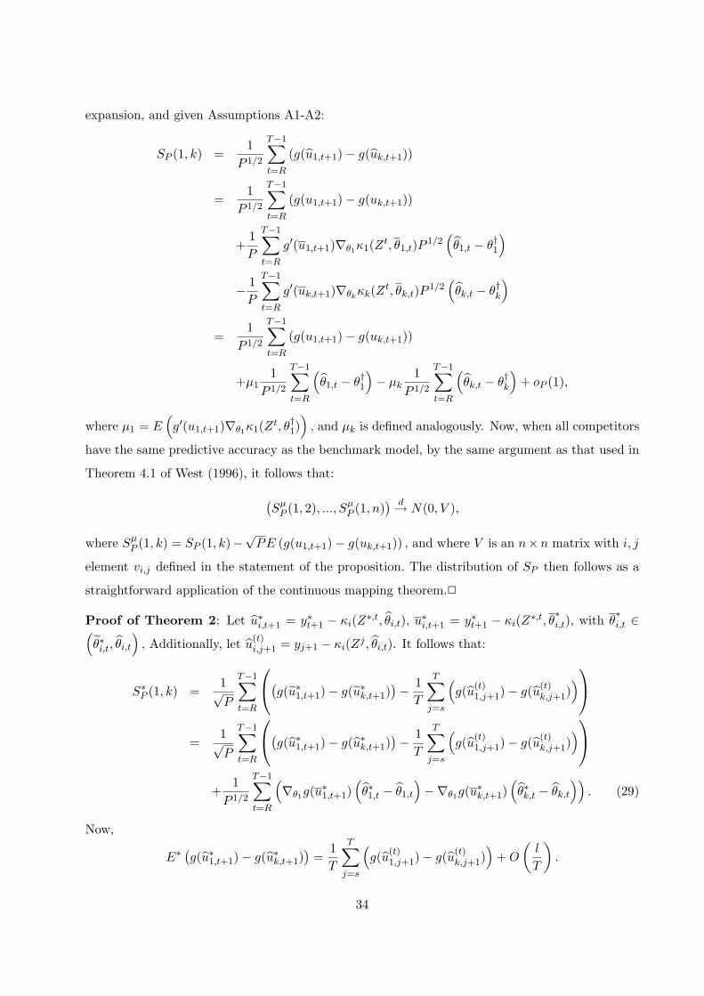
expansion, and given Assumptions A1-A2:

SP (1, k) =1

P 1/2

T−1∑t=R

(g(u1,t+1)− g(uk,t+1))

=1

P 1/2

T−1∑t=R

(g(u1,t+1)− g(uk,t+1))

+1P

T−1∑t=R

g′(u1,t+1)∇θ1κ1(Zt, θ1,t)P 1/2(θ1,t − θ†1

)− 1P

T−1∑t=R

g′(uk,t+1)∇θkκk(Zt, θk,t)P 1/2

(θk,t − θ†k

)=

1P 1/2

T−1∑t=R

(g(u1,t+1)− g(uk,t+1))

+µ11

P 1/2

T−1∑t=R

(θ1,t − θ†1

)− µk

1P 1/2

T−1∑t=R

(θk,t − θ†k

)+ oP (1),

where µ1 = E(g′(u1,t+1)∇θ1κ1(Zt, θ†1)

), and µk is defined analogously. Now, when all competitors

have the same predictive accuracy as the benchmark model, by the same argument as that used in

Theorem 4.1 of West (1996), it follows that:

(Sµ

P (1, 2), ..., SµP (1, n)

) d→ N(0, V ),

where SµP (1, k) = SP (1, k)−

√PE (g(u1,t+1)− g(uk,t+1)) , and where V is an n×n matrix with i, j

element vi,j defined in the statement of the proposition. The distribution of SP then follows as a

straightforward application of the continuous mapping theorem.2

Proof of Theorem 2: Let u∗i,t+1 = y∗t+1 − κi(Z∗,t, θi,t), u∗i,t+1 = y∗t+1 − κi(Z∗,t, θ∗i,t), with θ

∗i,t ∈(

θ∗i,t, θi,t

), Additionally, let u(t)

i,j+1 = yj+1 − κi(Zj , θi,t). It follows that:

S∗P (1, k) =1√P

T−1∑t=R

(g(u∗1,t+1)− g(u∗k,t+1))− 1T

T∑j=s

(g(u(t)

1,j+1)− g(u(t)k,j+1)

)=

1√P

T−1∑t=R

(g(u∗1,t+1)− g(u∗k,t+1))− 1T

T∑j=s

(g(u(t)

1,j+1)− g(u(t)k,j+1)

)+

1P 1/2

T−1∑t=R

(∇θ1g(u

∗1,t+1)

(θ∗1,t − θ1,t

)−∇θ1g(u

∗k,t+1)

(θ∗k,t − θk,t

)). (29)

Now,

E∗(g(u∗1,t+1)− g(u∗k,t+1)

)=

1T

T∑j=s

(g(u(t)

1,j+1)− g(u(t)k,j+1)

)+O

(l

T

).

34

Thus, by Theorem 3.5 in Kunsch (1989), the first term on the second equality on the RHS of

(29) converges in P ∗−distribution to a zero mean normal random variable with variance equal to

limP→∞ V ar∗(

1√P

∑T−1t=R

(g(u∗1,t+1)− g(u∗k,t+1)

)), conditional on the sample and for all samples

except a subset with probability measure approaching zero. Now, by the same argument used in

the proof of Theorem 1:

V ar∗

(1√P

T−1∑t=R

(g(u∗1,t+1)− g(u∗k,t+1)

))= V ar

(1√P

T−1∑t=R

(g(u1,t+1)− g(uk,t+1))

)+ o(1) Pr−P.

This implies that the first term in the second equality on the RHS of (29) has the same lim-

iting distribution as 1√P

∑T−1t=R ((g(u1,t+1)− g(uk,t+1))− E (g(u1,t+1)− g(uk,t+1))) , conditional on

the sample, and for all samples except a subset with probability measure approaching zero. Fi-

nally, the last term in (29) has the same limiting distribution as µ11

P 1/2

∑T−1t=R

(θ∗1,t − θ1,t

)−

µk1

P 1/2

∑T−1t=R

(θ∗k,t − θk,t

), conditional on the sample, and for all samples except a subset with

probability measure approaching zero. The statement in the proposition then follows as a straight-

forward application of the continuous mapping theorem.2

Proof of Proposition 2: The proof follows directly from Theorem 1 in Corradi and Swanson

(2002).2

Proof of Theorem 3: Recall that g = q1. Additionally, let u∗1,t+1 = y∗t+1 −(

1 y∗t

)θ∗1,t,

u∗1,t+1 = y∗t+1 −(

1 y∗t

)θ1,t, u

∗1,t+1 = y∗t+1 −

(1 y∗t

)θ∗1,t, and u

(t)1,j+1 = yj+1 −

(1 yt

)θ1,t,

where θ∗1,t ∈(θ∗1,t, θ1,t

). It then follows that:

1P 1/2

T−1∑t=R

g′(u∗1,t+1)w(Z∗,t, γ)− 1T

T−1∑j=2

g′(u(t)1,j+1)w(Zj , γ)

=

1P 1/2

T−1∑t=R

g′(u∗1,t+1)w(Z∗,t, γ)− 1T

T−1∑j=2

g′(u(t)1,j+1)w(Zj , γ)

+

1P 1/2

T−1∑t=R

(∇θg

′(u∗1,t+1)w(Z∗,t, γ)) (θ∗1,t − θ1,t

). (30)

First, note that the first term on the RHS of the last equality in (30) has the same limiting

distribution as1

P 1/2

∑T−1t=R

(g′(u1,t+1)w(Zt, γ)− E

(g′(u1,t+1)w(Zt, γ)

)), pointwise in γ. Further, note that stochas-

tic equicontinuity on Γ can be shown using the same approach as that used in the proof of Theo-

rem 2 in Corradi and Swanson (2002). Therefore, under H0, any continuous functional over Γ of1

P 1/2

∑T−1t=R

(g′(u∗1,t+1)w(Z∗,t, γ)− 1

T

∑T−1j=2 g

′(u(t)1,j+1)w(Zj , γ)

)has the same limiting distribution of

35

the same functional of 1P 1/2

∑T−1t=R

(g′(u1,t+1)w(Zt, γ)− E

(g′(u1,t+1)w(Zt, γ)

)). Finally, note that

1P 1/2

∑T−1t=R

(∇θg

′(u∗1,t+1)w(Z∗,t, γ)) (θ∗1,t − θ1,t

)properly captures the contribution of recursive pa-

rameter estimation error to the covariance kernel.2

36

9 References

Altissimo, F. and V. Corradi, (2002), Bounds for Inference with Nuisance Parameters Present onlyunder the Alternative”, Econometrics Journal, 5, 494-518.

Andrews, D.W.K., (2002), Higher-Order Improvements of a Computationally Attractive k−stepBootstrap for Extremum Estimators, Econometrica, 70, 119-162.

Andrews, D.W.K., (2004), The Block-Block Bootstrap: Improved Asymptotic Refinements, Econo-metrica, 72, 673-700.

Bachmeier, L. and N.R. Swanson, (2005), Predicting Inflation: Does The Quantity Theory Help?,Economic Inquiry, 43, 570-585.

Bierens, H.B., (1982): Consistent model specification tests, Journal of Econometrics, 20, 105-134.

Bierens, H.B., (1990): A Conditional Moment Test of Functional Form, Econometrica , 58, 1443-1458.

Bierens, H.J. and W. Ploberger, (1997): Asymptotic theory of integrated conditional moment tests,Econometrica, 65, 1129-1152.

Carlstein, E. (1986), The Use of Subseries Methods for Estimating the Variance of a GeneralStatistic from a Stationary Time Series, Annals of Statistics, 14, 1171-1179.

Chao, J.C., V. Corradi, and N.R. Swanson (2001), An Out of Sample Test for Granger Causality”,Macroeconomic Dynamics, v.5, 598-620.

Christoffersen, P. and F.X. Diebold, (1996), Further Results on Forecasting and Model Selectionunder Asymmetric Loss, Journal of Applied Econometrics, 11, 561-572.

Christoffersen, P. and F.X. Diebold, (1997), Optimal Prediction Under Asymmetric Loss, Econo-metric Theory, 13, 808-817.

Clark, T.E., and M.W., McCracken, (2001), Tests of Equal Forecast Accuracy and Encompassingfor Nested Models, Journal of Econometrics 105, 85-110.

Clark, T.E., and M.W., McCracken (2004), Evaluating Long-Horizon Forecasts, Working Paper,University of Missouri-Columbia.

Corradi, V., (1999), Deciding between I(0) and I(1) via FLIL-Based Bounds, Econometric Theory,15, 643-663.

Corradi, V. and N.R. Swanson, (2002), A Consistent Test for Out of Sample Nonlinear PredictiveAbility, Journal of Econometrics, 110, 353-381.

Corradi, V. and N.R. Swanson, (2004a), “Predictive Density Evaluation”, in: Handbook of Eco-nomic Forecasting, eds. Clive W.J. Granger, Graham Elliot and Allan Timmerman, Elsevier,Amsterdam, forthcoming.

Corradi, V. and N.R. Swanson, (2004b), Some Recent Developments in Predictive Accuracy Testingwith Nested Models and (Generic) Nonlinear Alternatives”, International Journal of Forecasting,20, 185-199.

Corradi, V. and N.R. Swanson, (2005), “Predictive Density and Confidence Intervals AccuracyTests”, Journal of Econometrics, forthcoming.

Diebold, F.X., and R.S. Mariano, (1995), Comparing Predictive Accuracy, Journal of Business andEconomic Statistics, 13, 253-263.

Diebold, F.X. and C. Chen, (1996), Testing Structural Stability with Endogenous Breakpoint: ASize Comparison of Analytic and Bootstrap Procedures, Journal of Econometrics, 70, 221-241.

Elliott, G. and A. Timmerman, (2004a), Optimal Forecast Combinations Under General LossFunctions and Forecast Error Distributions, Journal of Econometrics, 122, 47-79.

37

Elliott, G. and A. Timmerman, (2004b), Optimal Forecast Combination Under Regime Switching,International Economic Review, forthcoming.

Fitzenberger, B. (1997), The Moving Block Bootstrap and Robust Inference for Linear Least Squareand Quantile Regressions, Journal of Econometrics, 82, 235-287.

Gallant, A.R. and H. White, (1988), A Unified Theory of Estimation and Inference for NonlinearDynamic Models, Blackwell, Oxford.

Giacomini, R., and H. White (2003), Conditional Tests for Predictive Ability, manuscript, Univer-sity of California, San Diego.

Goncalves, S., and H. White, (2004), Maximum Likelihood and the Bootstrap for Nonlinear Dy-namic Models, Journal of Econometrics, 119, 199-219.

Granger, C.W.J., (1993), On the Limitations of Comparing Mean Squared Forecast Errors: Com-ment, Journal of Forecasting, 12, 651-652.

Granger, C.W.J., (1999), Outline of Forecast Theory Using Generalized Cost Functions, SpanishEconomic Review, 1, 161-173.

Hall, P., and J.L. Horowitz, (1996), Bootstrap Critical Values for Tests Based on GeneralizedMethod of Moments Estimators, Econometrica, 64, 891-916.

Hansen, B.E., (1996), Inference When a Nuisance Parameter is Not Identified Under the NullHypothesis, Econometrica, 64, 413-430.

Harvey, D.I., S.J. Leybourne and P. Newbold, (1997), Tests for Forecast Encompassing, Journal ofBusiness and Economic Statistics, 16, 254-259.Inoue, A., (2001), Testing for Distributional Change in Time Series, Econometric Theory, 17, 156-187.

Inoue, A., and M. Shintani, (2004), Bootstrapping GMM Estimators for Time Series, Journal ofEconometrics, forthcoming.

Inoue, A., and B. Rossi, (2004), Recursive Predictive Ability Tests for Real Time Data, WorkingPaper, Duke University and NC State.

Inoue, A. and L. Kilian, (2004), In-Sample and Out-of-Sample Tests of Predictability: Which OneShould We Use?, Econometric Reviews, 23, 371-402.

Inoue, A. and L. Kilian, (2005), On the Selection of Forecasting Models, Journal of Econometrics,forthcoming.

Kilian, L., (1999), Exchange Rate and Monetary Fundamentals: What do we Learn from Long-Horizon Regressions, Journal of Applied Econometrics, 14, 491-510.

Kilian, L. and M.P. Taylor, (2003), Why is it so Difficult to Beat the Random Walk Forecast ofExchange Rates?, Journal of International Economics, 60, 85-107.

Kunsch H.R., (1989), The Jackknife and the Bootstrap for General Stationary Observations, Annalsof Statistics, 17, 1217-1241.

Lahiri, S.N., (1999), Theoretical Comparisons of Block Bootstrap Methods, Annals of Statistics,27, 386-404.

Linton, O., E. Maasoumi and Y.J. Whang, (2005), Consistent Testing for Stochastic DominanceUnder General Sampling Schemes, Review of Economic Studies, 72, 735-766.

McCracken, M.W., (2004), Asymptotics for Out of Sample Tests of Causality, Working Paper,University of Missouri-Columbia.

McCracken. M.W., and S. Sapp, (2005), Evaluating the Predictive Ability of Exchange RatesUsing Long Horizon Regressions: Mind your p’s and q’s. Journal of Money, Credit and Banking,37, 473-494.

38

Newey, W.K. and K.D. West, (1987), A Simple Positive-Definite Heteroskedasticity and Autocor-relation Consistent Covariance Matrix, Econometrica, 55, 703-708.

Politis, D.N. and J.P. Romano, (1994), The Stationary Bootstrap, Journal of the American Statis-tical Association, 89, 1303-1313.

Politis, D.N., J.P. Romano and M. Wolf, (1999), Subsampling, Springer and Verlag, New York.

Schorfheide, F., (2005), VAR Forecasting under Misspecification, Journal of Econometrics, 128,99-136.

Stinchcombe, M.B. and H. White, (1998), Consistent Specification Testing with Nuisance Parame-ters Present Only Under the Alternative, Econometric Theory, 14, 3, 295-325.

Swanson, N.R. and H. White, (1997), A Model Selection Approach to Real-Time MacroeconomicForecasting using Linear Models and Artificial Neural Networks, Review of Economics and Statis-tics, 79, 540-550.

Weiss, A., (1996) Estimating Time Series Models Using the Relevant Cost Function, Journal ofApplied Econometrics, 11, 539-560.

West, K., (1996), Asymptotic Inference About Predictive Ability, Econometrica, 64, 1067-1084.

White, H., (2000), A Reality Check for Data Snooping, Econometrica, 68, 1097-1126.

Wooldridge, J.M. and H. White, (1988), Some Invariance Principles and Central Limit Theoremsfor Dependent and Heterogeneous Processes, Econometric Theory, 4, 210-230.

Zellner, A., (1986), Bayesian Estimation and Prediction Using Asymmetric Loss Function, Journalof the American Statistical Association, 81, 446-451.

39

Table 1: Test Statistics, Sampling Scheme, and Data Generating Processes Used inEmpirical and Monte Carlo Sections

Panel A: Test Statistic Mnemonics and Definitions

F – The standard Wald version of the in-sample F-test is calculated using the entire sample of T observations. In particular,

we use: F = T�PT

t=1 bu21,t −

PTt=1 bu2

2,t)/PT

t=1 bu22,t

�, where bu1,t and bu2,t are the in-sample residuals associated with least

squares estimation of the small and big models, respectively, and where T denotes the sample size.CM – The Clark and McCracken (2004) test outlined in Section 5.DM – The Diebold and Mariano (1995) test outlined in Section 5.CS – The Corradi and Swanson (2002) test outlined in Section 4.CCS – The Chao, Corradi and Swanson (2001) test discussed in Section 5.

Panel B: Data Generating Processes Used in Monte Carlo Experiments

xt = a1 + a2xt−1 + u1,t, u1,t ∼ iidN(0, 1)wt = a1 + a3wt−1 + u2,t, u2,t ∼ iidN(0, 1)Size1: yt = a1 + a2yt−1 + a4wt−1 + u3,t, u3,t ∼ iidN(0, 1)Size2: yt = a1 + a2yt−1 + a4wt−1 + a3u3,t−1 + u3,t

Power1 : yt = a1 + a2yt−1 + 2 exp(tan−1(xt−1/2)) + a4wt−1 + u3,tPower2 : yt = a1 + a2yt−1 + 2xt−1 + a4wt−1 + u3,t

Power3 : yt = a1 + a2yt−1 + 2xt−11{xt−1 > a1/(1− a2)}+ a4wt−1 + u3,t

Power4 : yt = a1 + a2yt−1 + 2 exp(tan−1(xt−1/2)) + a4wt−1 + a3u3,t−1 + u3,tPower5: yt = a1 + a2yt−1 + 2xt−1 + a4wt−1 + a3u3,t−1 + u3,t

Power6: yt = a1 + a2yt−1 + 2xt−11{xt−1 > a1/(1− a2)}+ a4wt−1 + a3u3,t−1 + u3,t.Power7 : yt = a1 + a2yt−1 + 2 exp(xt−1) + a4wt−1 + u3,t

Power8 : yt = a1 + a2yt−1 + 2x2t−1 + a4wt−1 + u3,t

Power9 : yt = a1 + a2yt−1 + 2|xt−1|+ a4wt−1 + u3,t

Power10 : yt = a1 + a2yt−1 + 2 exp(xt−1) + a4wt−1 + a3u3,t−1 + u3,t

Power11: yt = a1 + a2yt−1 + 2x2t−1 + a4wt−1 + a3u3,t−1 + u3,t

Power12: yt = a1 + a2yt−1 + 2|xt−1|+ a4wt−1 + a3u3,t−1 + u3,t.Note that the benchmark or “small” model in our test statistic calculations is always yt = α + βyt−1 + εt;

and the “big” model is the same, but with xt−1 added as an additional regressor. Note further that wt−1 is neverused in test statistic forecast model construction. Hence, the difference between the variance of the “small” modeland the optimal variance of the “big” model simply the variance of the nonlinear term in the true DGP (whenver thetrue DGP is either Power1-Power12).

40

Table 2: Rejection Frequencies of CS Test with a4 = 0, T = 600, P = 0.5T ∗

Model Recur Block Bootstrap BB, no PEE, no adj Block Bootstrap Kilian BootPanel A: a2 = 0.3

l = 2 l = 5 l = 10 l = 2 l = 5 l = 10 l = 2 l = 5 l = 10Size1 0.11 0.11 0.11 0.06 0.03 0.01 0.00 0.00 0.00 0.09Size2 0.06 0.08 0.09 0.01 0.04 0.04 0.00 0.00 0.00 0.01

Power1 0.77 0.98 0.98 0.01 0.99 0.98 0.99 0.96 0.93 1.00Power2 0.84 0.99 0.98 0.01 1.00 0.98 1.00 0.95 0.94 1.00Power3 0.81 0.97 0.98 0.03 1.00 0.97 1.00 0.95 0.93 1.00Power4 0.74 0.97 0.99 0.00 0.99 0.98 0.98 0.94 0.92 1.00Power5 0.83 0.98 0.99 0.01 1.00 0.98 1.00 0.96 0.94 1.00Power6 0.81 0.98 0.99 0.01 1.00 0.97 1.00 0.95 0.93 1.00Power7 0.56 0.73 0.74 0.00 0.76 0.78 0.77 0.74 0.71 0.99Power8 0.68 0.89 0.92 0.00 0.96 0.91 0.97 0.88 0.85 1.00Power9 0.81 0.99 1.00 0.03 1.00 0.97 1.00 0.96 0.93 1.00Power10 0.56 0.72 0.77 0.00 0.74 0.78 0.76 0.74 0.70 0.99Power11 0.70 0.88 0.92 0.00 0.95 0.90 0.97 0.86 0.83 1.00Power12 0.79 0.97 0.98 0.01 1.00 0.97 1.00 0.96 0.92 1.00

Panel B: a2 = 0.6l = 4 l = 10 l = 20 l = 4 l = 10 l = 20 l = 4 l = 10 l = 20

Size1 0.09 0.12 0.12 0.03 0.04 0.03 0.00 0.00 0.00 0.00Size2 0.05 0.07 0.09 0.01 0.04 0.04 0.00 0.00 0.00 0.00

Power1 0.89 0.95 0.97 0.02 0.98 0.95 0.93 0.88 0.86 0.99Power2 0.92 0.96 0.97 0.07 0.99 0.95 0.94 0.91 0.90 1.00Power3 0.92 0.96 0.96 0.11 0.99 0.94 0.94 0.90 0.88 1.00Power4 0.89 0.95 0.96 0.01 0.98 0.96 0.92 0.87 0.88 0.99Power5 0.92 0.97 0.98 0.04 0.99 0.95 0.94 0.91 0.90 1.00Power6 0.92 0.95 0.96 0.07 0.99 0.96 0.94 0.89 0.89 1.00Power7 0.55 0.59 0.66 0.00 0.61 0.65 0.57 0.59 0.61 0.73Power8 0.83 0.89 0.90 0.01 0.94 0.89 0.87 0.83 0.80 1.00Power9 0.93 0.97 0.99 0.11 0.99 0.96 0.95 0.90 0.87 1.00Power10 0.55 0.62 0.68 0.00 0.63 0.66 0.53 0.59 0.62 0.75Power11 0.83 0.87 0.88 0.01 0.93 0.90 0.88 0.81 0.79 0.99Power12 0.93 0.97 0.98 0.09 0.99 0.96 0.95 0.90 0.87 1.00

Panel C: a2 = 0.9l = 10 l = 20 l = 50 l = 10 l = 20 l = 50 l = 10 l = 20 l = 50

Size1 0.06 0.07 0.08 0.02 0.03 0.03 0.00 0.00 0.00 0.00Size2 0.02 0.04 0.06 0.00 0.01 0.01 0.00 0.00 0.00 0.01

Power1 0.68 0.78 0.84 0.03 0.88 0.88 0.67 0.73 0.75 0.71Power2 0.71 0.78 0.87 0.08 0.90 0.86 0.68 0.71 0.73 0.90Power3 0.73 0.81 0.86 0.13 0.92 0.88 0.70 0.71 0.74 0.85Power4 0.65 0.73 0.85 0.01 0.83 0.89 0.64 0.68 0.75 0.69Power5 0.72 0.78 0.88 0.07 0.92 0.88 0.69 0.71 0.75 0.89Power6 0.74 0.79 0.87 0.13 0.92 0.87 0.70 0.69 0.74 0.86Power7 0.41 0.44 0.53 0.00 0.42 0.55 0.35 0.42 0.51 0.45Power8 0.66 0.72 0.81 0.11 0.82 0.81 0.61 0.66 0.70 0.87Power9 0.73 0.80 0.88 0.11 0.93 0.88 0.69 0.72 0.74 0.85Power10 0.40 0.46 0.52 0.00 0.44 0.54 0.34 0.43 0.52 0.43Power11 0.63 0.72 0.81 0.06 0.83 0.81 0.64 0.63 0.70 0.86Power12 0.76 0.81 0.87 0.09 0.92 0.87 0.72 0.70 0.74 0.86

∗ Notes: All entries are rejection frequencies of the null hypothesis of equal predictive accuracy based on 10% nominal sizecritical values constructed using the bootstrap approaches discussed above, where l denotes the block length, and empiricalbootstrap distributions are constructed using 100 bootstrap statistics. In particular, “Recur Block Bootstrap” is the bootstrapdeveloped in this paper, “BB, no PEE, no adj” is a naive block bootstrap where no parameter estimation error is assumed,and no recentering (i.e. adjustment) is done in parameter estimation or bootstrap statistic construction, “Block Bootstrap” isthe usual block bootstrap that allows for parameter estimation error, but does not recenter parameter estimates or bootstrapstatistics, AND “Kilian Boot” is the Kilian (1999) parametric bootstrap implemented in Clark and McCracken (2004) andMcCracken and Sapp (2004).. For all models denoted Poweri, i = 1, ..., 6, data are generated with (non) linear Grangercausality (see above for further discussion of DGPs. In all experiments, the ex ante forecast period is of length P , which is setequal to (1/2)T , where T is the sample size. All models are estimated recursively, so that parameter estimates are updatedbefore each new prediction is constructed. All reported results are based on 500 Monte Carlo simulations. See Table 1 andSection 5 for further details.

41

Table 3: Rejection Frequencies of CS Test with a4 = 1, T = 600, P = 0.5T ∗

Model Recur Block Bootstrap BB, no PEE, no adj Block Bootstrap Kilian BootPanel A: a2 = 0.3

l = 2 l = 5 l = 10 l = 2 l = 5 l = 10 l = 2 l = 5 l = 10Size1 0.11 0.11 0.10 0.03 0.06 0.02 0.00 0.00 0.00 0.04Size2 0.07 0.09 0.11 0.01 0.07 0.04 0.00 0.00 0.00 0.01

Power1 0.61 0.91 0.93 0.00 0.96 0.95 0.90 0.90 0.86 0.98Power2 0.78 0.97 0.98 0.00 0.99 0.96 0.99 0.94 0.90 1.00Power3 0.79 0.97 0.97 0.00 0.98 0.96 0.98 0.94 0.90 1.00Power4 0.59 0.91 0.95 0.00 0.95 0.95 0.88 0.91 0.86 0.98Power5 0.79 0.96 0.98 0.00 0.99 0.97 0.99 0.94 0.90 1.00Power6 0.76 0.97 0.98 0.00 0.99 0.96 0.99 0.94 0.91 1.00Power7 0.60 0.75 0.77 0.00 0.74 0.79 0.76 0.74 0.72 0.95Power8 0.70 0.86 0.88 0.00 0.94 0.88 0.97 0.85 0.82 0.99Power9 0.76 0.95 0.97 0.00 0.98 0.95 0.98 0.93 0.89 1.00Power10 0.61 0.75 0.78 0.00 0.74 0.78 0.78 0.73 0.72 0.96Power11 0.70 0.86 0.89 0.00 0.94 0.89 0.96 0.85 0.81 0.99Power12 0.77 0.96 0.98 0.00 0.99 0.96 0.98 0.93 0.90 0.99

Panel B: a2 = 0.6l = 4 l = 10 l = 20 l = 4 l = 10 l = 20 l = 4 l = 10 l = 20

Size1 0.07 0.08 0.10 0.02 0.06 0.02 0.00 0.00 0.00 0.00Size2 0.05 0.07 0.09 0.02 0.06 0.03 0.00 0.00 0.00 0.00

Power1 0.78 0.87 0.91 0.00 0.93 0.91 0.83 0.79 0.80 0.92Power2 0.88 0.94 0.95 0.02 0.98 0.94 0.90 0.86 0.85 0.99Power3 0.91 0.95 0.96 0.03 0.97 0.94 0.92 0.88 0.86 0.99Power4 0.74 0.87 0.91 0.00 0.92 0.91 0.83 0.81 0.81 0.90Power5 0.90 0.94 0.96 0.00 0.98 0.95 0.92 0.86 0.86 0.99Power6 0.90 0.95 0.96 0.03 0.97 0.95 0.91 0.88 0.85 1.00Power7 0.55 0.62 0.67 0.00 0.61 0.67 0.55 0.58 0.63 0.75Power8 0.78 0.85 0.86 0.01 0.93 0.85 0.84 0.75 0.72 0.97Power9 0.90 0.96 0.96 0.05 0.97 0.95 0.93 0.84 0.85 0.98Power10 0.54 0.61 0.66 0.00 0.62 0.67 0.53 0.58 0.62 0.75Power11 0.78 0.83 0.88 0.01 0.91 0.86 0.83 0.75 0.74 0.97Power12 0.89 0.95 0.96 0.03 0.97 0.96 0.92 0.86 0.83 0.98

Panel C: a2 = 0.9l = 10 l = 20 l = 50 l = 10 l = 20 l = 50 l = 10 l = 20 l = 50

Size1 0.02 0.05 0.05 0.00 0.03 0.02 0.00 0.00 0.00 0.00Size2 0.02 0.02 0.03 0.00 0.02 0.02 0.00 0.00 0.00 0.00

Power1 0.53 0.63 0.76 0.00 0.63 0.84 0.50 0.60 0.69 0.55Power2 0.69 0.76 0.84 0.02 0.88 0.85 0.68 0.71 0.72 0.82Power3 0.72 0.80 0.86 0.05 0.91 0.86 0.72 0.74 0.75 0.81Power4 0.49 0.61 0.75 0.00 0.52 0.83 0.43 0.60 0.68 0.56Power5 0.69 0.76 0.82 0.01 0.88 0.85 0.66 0.69 0.74 0.82Power6 0.73 0.76 0.84 0.07 0.89 0.86 0.71 0.70 0.74 0.81Power7 0.40 0.44 0.50 0.01 0.39 0.52 0.34 0.43 0.49 0.41Power8 0.61 0.66 0.77 0.08 0.81 0.77 0.61 0.63 0.66 0.85Power9 0.70 0.75 0.82 0.10 0.88 0.84 0.66 0.67 0.70 0.85Power10 0.41 0.45 0.53 0.01 0.42 0.56 0.33 0.43 0.51 0.40Power11 0.64 0.69 0.76 0.07 0.79 0.75 0.64 0.62 0.66 0.85Power12 0.68 0.77 0.85 0.08 0.88 0.85 0.66 0.68 0.71 0.82

∗ Notes: See notes to Table 2.

42

Table 4: Rejection Frequencies of Various Tests with a4 = 0, T = 600, P = 0.5T ∗

Model Assume π = 0 Assume π > 0 Kilian Bootstrap Recur Block BootstrapF DM CM DM CM F DM CM CCS CCS-l1 CCS-l2 CCS-l3

Panel A: a2 = 0.3Size1 0.24 0.01 0.05 0.09 0.09 0.08 0.10 0.10 0.08 0.22 0.22 0.20Size2 0.25 0.01 0.06 0.09 0.09 0.09 0.09 0.09 0.03 0.17 0.17 0.17

Power1 1.00 1.00 1.00 1.00 1.00 1.00 1.00 1.00 1.00 1.00 1.00 0.99Power2 1.00 1.00 1.00 1.00 1.00 1.00 1.00 1.00 1.00 1.00 1.00 1.00Power3 1.00 1.00 1.00 1.00 1.00 1.00 1.00 1.00 1.00 1.00 1.00 0.98Power4 1.00 1.00 1.00 1.00 1.00 1.00 1.00 1.00 1.00 1.00 1.00 0.99Power5 1.00 1.00 1.00 1.00 1.00 1.00 1.00 1.00 1.00 1.00 1.00 1.00Power6 1.00 1.00 1.00 1.00 1.00 1.00 1.00 1.00 1.00 1.00 1.00 0.98Power7 1.00 1.00 1.00 1.00 1.00 1.00 1.00 1.00 1.00 1.00 0.87 0.78Power8 1.00 1.00 1.00 1.00 1.00 1.00 1.00 1.00 1.00 1.00 1.00 0.95Power9 1.00 1.00 1.00 1.00 1.00 1.00 1.00 1.00 1.00 1.00 1.00 1.00Power10 1.00 1.00 1.00 1.00 1.00 1.00 1.00 1.00 1.00 0.99 0.87 0.78Power11 1.00 1.00 1.00 1.00 1.00 1.00 1.00 1.00 1.00 1.00 0.99 0.94Power12 1.00 1.00 1.00 1.00 1.00 1.00 1.00 1.00 1.00 1.00 1.00 1.00

Panel B: a2 = 0.6Size1 0.25 0.01 0.05 0.09 0.10 0.10 0.09 0.09 0.00 0.18 0.18 0.20Size2 0.27 0.02 0.06 0.11 0.10 0.10 0.10 0.10 0.00 0.12 0.15 0.17

Power1 1.00 1.00 1.00 1.00 1.00 1.00 1.00 1.00 1.00 1.00 0.97 0.96Power2 1.00 1.00 1.00 1.00 1.00 1.00 1.00 1.00 1.00 1.00 0.99 0.98Power3 1.00 1.00 1.00 1.00 1.00 1.00 1.00 1.00 1.00 1.00 0.97 0.94Power4 1.00 1.00 1.00 1.00 1.00 1.00 1.00 1.00 1.00 1.00 0.97 0.95Power5 1.00 1.00 1.00 1.00 1.00 1.00 1.00 1.00 1.00 1.00 0.98 0.98Power6 1.00 1.00 1.00 1.00 1.00 1.00 1.00 1.00 1.00 1.00 0.97 0.96Power7 1.00 1.00 1.00 1.00 1.00 1.00 0.96 0.98 1.00 0.84 0.68 0.64Power8 1.00 1.00 1.00 1.00 1.00 1.00 1.00 1.00 1.00 1.00 0.92 0.88Power9 1.00 1.00 1.00 1.00 1.00 1.00 1.00 1.00 1.00 1.00 0.98 0.96Power10 1.00 1.00 1.00 1.00 1.00 1.00 0.97 0.98 1.00 0.83 0.68 0.64Power11 1.00 1.00 1.00 1.00 1.00 1.00 1.00 1.00 1.00 1.00 0.93 0.88Power12 1.00 1.00 1.00 1.00 1.00 1.00 1.00 1.00 1.00 1.00 0.98 0.96

Panel C: a2 = 0.9Size1 0.25 0.01 0.06 0.09 0.10 0.10 0.07 0.07 0.00 0.14 0.17 0.20Size2 0.29 0.03 0.08 0.11 0.12 0.14 0.11 0.11 0.00 0.11 0.12 0.16

Power1 1.00 1.00 1.00 1.00 1.00 1.00 1.00 1.00 0.81 0.85 0.86 0.88Power2 1.00 1.00 1.00 1.00 1.00 1.00 1.00 1.00 0.93 0.90 0.90 0.92Power3 1.00 1.00 1.00 1.00 1.00 1.00 1.00 1.00 0.90 0.84 0.86 0.88Power4 1.00 1.00 1.00 1.00 1.00 1.00 1.00 1.00 0.82 0.85 0.86 0.89Power5 1.00 1.00 1.00 1.00 1.00 1.00 1.00 1.00 0.93 0.89 0.89 0.93Power6 1.00 1.00 1.00 1.00 1.00 1.00 1.00 1.00 0.91 0.82 0.85 0.88Power7 1.00 0.98 1.00 1.00 1.00 1.00 0.85 0.91 0.73 0.45 0.47 0.47Power8 1.00 1.00 1.00 1.00 1.00 1.00 1.00 1.00 0.93 0.79 0.78 0.80Power9 1.00 1.00 1.00 1.00 1.00 1.00 1.00 1.00 0.91 0.85 0.87 0.89Power10 1.00 0.98 1.00 1.00 1.00 1.00 0.84 0.92 0.74 0.47 0.45 0.47Power11 1.00 1.00 1.00 1.00 1.00 1.00 1.00 1.00 0.93 0.77 0.76 0.82Power12 1.00 1.00 1.00 1.00 1.00 1.00 1.00 1.00 0.91 0.84 0.86 0.88

∗ Notes: See notes to Table 2. Test statistics, denoted by F, DM, CM, CS, and CCS are summarized in Table 1. Block lengthsare denoted by l1, l2, and l3, so that CCS − l3 is the CCS test with block length l3. Block lengths corrspond to those usedin Table 2 and 3, so that for a2 = 0.3, l1, l2, l3=2,5,10. The block lengths for a2 = 0.6 and a2 = 0.9 are l1, l2, l3=4,10,20 andl1, l2, l3=10,20,50, respectively. π = 0 corresponds to the case where standard critical values based upon the assumption thatparameter estimation error vanishes asymptotically are used (i.e. π = limT−>∞P/R = 0). π > 0 corresponds to the casewhere nonstandard critical values (see McCracken (2004)) based upon the assumption that parameter estimation error doesnot vanish asymptotically are used (i.e. π = limT−>∞P/R > 0). In this case, we assume that π = 1.

43

Table 5: Rejection Frequencies of Various Tests with a4 = 1, T = 600, P = 0.5T ∗

Model Assume π = 0 Assume π > 0 Kilian Bootstrap Recur Block BootstrapF DM CM DM CM F DM CM CCS CCS-l1 CCS-l2 CCS-l3

Panel A: a2 = 0.3Size1 0.26 0.02 0.05 0.07 0.07 0.12 0.10 0.09 0.04 0.23 0.21 0.22Size2 0.27 0.02 0.05 0.09 0.07 0.11 0.09 0.09 0.02 0.16 0.19 0.22

Power1 1.00 1.00 1.00 1.00 1.00 1.00 1.00 1.00 1.00 1.00 0.99 0.97Power2 1.00 1.00 1.00 1.00 1.00 1.00 1.00 1.00 1.00 1.00 1.00 1.00Power3 1.00 1.00 1.00 1.00 1.00 1.00 1.00 1.00 1.00 1.00 1.00 0.99Power4 1.00 1.00 1.00 1.00 1.00 1.00 1.00 1.00 1.00 1.00 0.99 0.97Power5 1.00 1.00 1.00 1.00 1.00 1.00 1.00 1.00 1.00 1.00 1.00 1.00Power6 1.00 1.00 1.00 1.00 1.00 1.00 1.00 1.00 1.00 1.00 1.00 0.98Power7 1.00 1.00 1.00 1.00 1.00 1.00 1.00 1.00 1.00 1.00 0.88 0.76Power8 1.00 1.00 1.00 1.00 1.00 1.00 1.00 1.00 1.00 1.00 0.98 0.93Power9 1.00 1.00 1.00 1.00 1.00 1.00 1.00 1.00 1.00 1.00 1.00 0.98Power10 1.00 1.00 1.00 1.00 1.00 1.00 1.00 1.00 1.00 1.00 0.88 0.76Power11 1.00 1.00 1.00 1.00 1.00 1.00 1.00 1.00 1.00 1.00 0.98 0.93Power12 1.00 1.00 1.00 1.00 1.00 1.00 1.00 1.00 1.00 1.00 1.00 0.98

Panel B: a2 = 0.6Size1 0.26 0.02 0.05 0.11 0.08 0.10 0.09 0.09 0.01 0.15 0.17 0.20Size2 0.27 0.02 0.06 0.09 0.08 0.11 0.10 0.10 0.00 0.10 0.16 0.18

Power1 1.00 1.00 1.00 1.00 1.00 1.00 1.00 1.00 1.00 0.99 0.94 0.89Power2 1.00 1.00 1.00 1.00 1.00 1.00 1.00 1.00 1.00 1.00 0.99 0.97Power3 1.00 1.00 1.00 1.00 1.00 1.00 1.00 1.00 1.00 0.99 0.96 0.94Power4 1.00 1.00 1.00 1.00 1.00 1.00 1.00 1.00 1.00 0.98 0.93 0.91Power5 1.00 1.00 1.00 1.00 1.00 1.00 1.00 1.00 1.00 1.00 0.99 0.96Power6 1.00 1.00 1.00 1.00 1.00 1.00 1.00 1.00 1.00 1.00 0.97 0.95Power7 1.00 1.00 1.00 1.00 1.00 1.00 0.97 0.99 0.99 0.82 0.68 0.63Power8 1.00 1.00 1.00 1.00 1.00 1.00 1.00 1.00 1.00 0.98 0.90 0.87Power9 1.00 1.00 1.00 1.00 1.00 1.00 1.00 1.00 1.00 0.99 0.97 0.94Power10 1.00 1.00 1.00 1.00 1.00 1.00 0.96 0.99 0.99 0.80 0.66 0.63Power11 1.00 1.00 1.00 1.00 1.00 1.00 1.00 1.00 1.00 0.98 0.91 0.87Power12 1.00 1.00 1.00 1.00 1.00 1.00 1.00 1.00 1.00 0.99 0.96 0.95

Panel C: a2 = 0.9Size1 0.27 0.03 0.08 0.12 0.12 0.13 0.09 0.11 0.00 0.09 0.12 0.15Size2 0.27 0.03 0.09 0.11 0.12 0.14 0.11 0.13 0.00 0.07 0.11 0.16

Power1 1.00 1.00 1.00 1.00 1.00 1.00 1.00 1.00 0.71 0.76 0.77 0.82Power2 1.00 1.00 1.00 1.00 1.00 1.00 1.00 1.00 0.89 0.86 0.88 0.89Power3 1.00 1.00 1.00 1.00 1.00 1.00 1.00 1.00 0.88 0.85 0.84 0.86Power4 1.00 1.00 1.00 1.00 1.00 1.00 1.00 1.00 0.72 0.71 0.77 0.81Power5 1.00 1.00 1.00 1.00 1.00 1.00 1.00 1.00 0.90 0.86 0.85 0.89Power6 1.00 1.00 1.00 1.00 1.00 1.00 1.00 1.00 0.88 0.81 0.82 0.85Power7 1.00 0.96 1.00 0.98 1.00 1.00 0.85 0.93 0.74 0.46 0.43 0.46Power8 1.00 1.00 1.00 1.00 1.00 1.00 1.00 1.00 0.93 0.73 0.74 0.76Power9 1.00 1.00 1.00 1.00 1.00 1.00 1.00 1.00 0.89 0.79 0.82 0.84Power10 1.00 0.96 1.00 0.98 1.00 1.00 0.84 0.93 0.74 0.46 0.44 0.48Power11 1.00 1.00 1.00 1.00 1.00 1.00 1.00 1.00 0.93 0.74 0.75 0.75Power12 1.00 1.00 1.00 1.00 1.00 1.00 1.00 1.00 0.88 0.80 0.81 0.85

∗ Notes: See notes to Table 4.

44

Table 6: Mean Square Forecast Errors Based Indicating the Marginal Predictive

Content of Unemployment for the CPI∗

Start Year Case 1 Case 2small model big model big model

1965 0.6239 0.6316 0.62891966 0.6329 0.6413 0.63681967 0.6335 0.6449 0.63701968 0.6363 0.6511 0.64031969 0.6363 0.6591 0.63991970 0.6267 0.6599 0.63051971 0.6295 0.6596 0.63631972 0.6438 0.6703 0.65071973 0.6564 0.6816 0.66361974 0.5603 0.5854 0.56501975 0.4929 0.5038 0.49931976 0.4849 0.4864 0.49161977 0.4953 0.4963 0.50261978 0.4933 0.4944 0.49791979 0.4882 0.4900 0.49051980 0.4598 0.4619 0.46101981 0.4226 0.4267 0.42461982 0.4158 0.4213 0.41781983 0.3810 0.3813 0.38201984 0.3799 0.3799 0.38151985 0.3873 0.3870 0.38871986 0.3982 0.3977 0.39951987 0.3751 0.3740 0.37551988 0.3881 0.3870 0.38871989 0.4008 0.3996 0.40181990 0.4102 0.4089 0.41101991 0.3796 0.3781 0.38141992 0.3915 0.3897 0.39301993 0.4117 0.4093 0.41311994 0.4329 0.4301 0.43461995 0.4559 0.4528 0.4586

∗ Notes: Mean square forecast errors (multiplied by 100000) are reported for two models (small which contains only lags ofinflation, and big which contains lags of inflation and unemployment). Case 1 refers to a big model that is specified usinginflation and unemployment, and Case 2 refers to the same, but specified using inflation and differenced unemployment. Allpredictions are of 1-step ahead inflation, and predictive periods begin in the year given in the first column of entries in thetable. All estmation and prediction is done recursively, as detailed in Section 6.

45

Table 7: Tests for the Marginal Predictive Content of Unemployment for the CPI∗

Test Statistic Prediction Period Begins 1970:1 Prediction Period Begins 1984:1Unem ∆Unem Unem ∆Unem

CS (Recur Block Bootstrap) reject reject no reject no rejectCS (Kilian Bootstrap) reject reject no reject no rejectCCS (Recur Block Bootstrap) reject reject reject no rejectCCS (Kilian Bootstrap) no reject no reject no reject no rejectF no reject no reject no reject no rejectDM (Kilian Bootstrap) no reject no reject no reject no rejectCM (Kilian Bootstrap) no reject no reject no reject no reject

∗ Notes: Entries denote either rejection (reject), or failure to reject (no reject) the null hypothesis that unemployment (columns2,4) or differenced unemployment (columns 3,5) has no marginal predictive content for core U.S. CPI. Starred entries denotenominal 10% level test rejection based on the use of critical values constructed using the approach signified using the mnemonicin brackets in the first column of the table. Explanation of these mnemonics are given in the notes to Table 2 and 4. All modelsuse monthly data and all predictions are 1-step ahead and are constructed using recursively estimated models. Results aregiven for predictions periods beginning with either 1970:1 or 1984:1 and ending in 2004:12. Estimation periods always begin in1955:1. See Section 6 for complete details. has

46