Lecture 6: Bootstrapping

36-402, Advanced Data Analysis

31 January 2013

The Big Picture

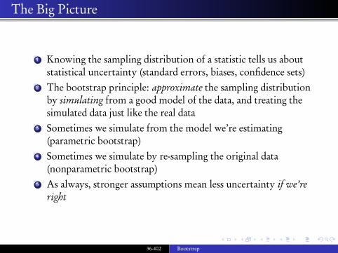
1 Knowing the sampling distribution of a statistic tells us aboutstatistical uncertainty (standard errors, biases, confidence sets)

2 The bootstrap principle: approximate the sampling distributionby simulating from a good model of the data, and treating thesimulated data just like the real data

3 Sometimes we simulate from the model we’re estimating(parametric bootstrap)

4 Sometimes we simulate by re-sampling the original data(nonparametric bootstrap)

5 As always, stronger assumptions mean less uncertainty if we’reright

36-402 Bootstrap

Statistical Uncertainty

Re-run the experiment (survey, census, . . . ) and we get more or lessdifferent data∴ everything we calculate from data (estimates, test statistics,policies, . . . ) will change from trial to trial as wellThis variability is (the source of) statistical uncertaintyQuantifying this is a way of being honest about what we do and donot know

36-402 Bootstrap

Measures of Statistical Uncertainty

Standard error = standard deviation of an estimatorcould equally well use median absolute deviation, etc.

p-value = Probability we’d see a signal this big if there was just noiseConfidence region = All the parameter values we can’t reject at lowerror rates:

1 Either the true parameter is in the confidence region2 or we are very unlucky3 or our model is wrong

etc.

36-402 Bootstrap

The Sampling Distribution Is the Source of All Knowledge

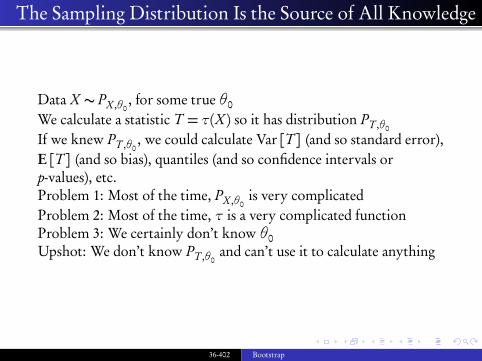
Data X ∼ PX,θ0, for some true θ0

We calculate a statistic T = τ(X) so it has distribution PT ,θ0

If we knew PT ,θ0, we could calculate Var[T ] (and so standard error),

E[T ] (and so bias), quantiles (and so confidence intervals orp-values), etc.Problem 1: Most of the time, PX,θ0

is very complicatedProblem 2: Most of the time, τ is a very complicated functionProblem 3: We certainly don’t know θ0Upshot: We don’t know PT ,θ0

and can’t use it to calculate anything

36-402 Bootstrap

The Solution

Classically (≈ 1900–≈ 1975): Restrict the model and the statisticuntil you can calculate the sampling distribution, at least for verylarge nModern (≈ 1975–): Use complex models and statistics, but simulatecalculating the statistic on the modelsome use of this idea back to the 1940s at least

36-402 Bootstrap

The Bootstrap Principle

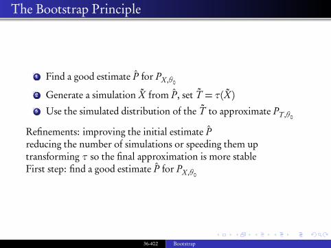
1 Find a good estimate P for PX,θ0

2 Generate a simulation X from P, set T = τ(X)3 Use the simulated distribution of the T to approximate PT ,θ0

Refinements: improving the initial estimate Preducing the number of simulations or speeding them uptransforming τ so the final approximation is more stableFirst step: find a good estimate P for PX,θ0

36-402 Bootstrap

Parametric Bootstrap

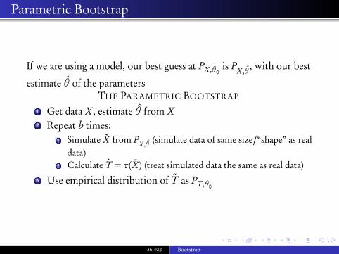
If we are using a model, our best guess at PX,θ0is PX,θ, with our best

estimate θ of the parametersTHE PARAMETRIC BOOTSTRAP

1 Get data X, estimate θ from X2 Repeat b times:

1 Simulate X from PX,θ (simulate data of same size/“shape” as realdata)

2 Calculate T = τ(X) (treat simulated data the same as real data)3 Use empirical distribution of T as PT ,θ0

36-402 Bootstrap

Concrete Example

Is Moonshine over-weight?

36-402 Bootstrap

Switch to R

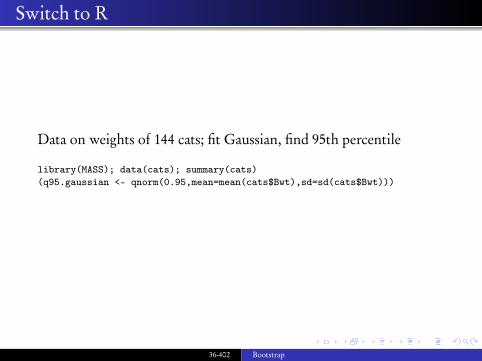
Data on weights of 144 cats; fit Gaussian, find 95th percentile

library(MASS); data(cats); summary(cats)(q95.gaussian <- qnorm(0.95,mean=mean(cats$Bwt),sd=sd(cats$Bwt)))

36-402 Bootstrap

Switch to R

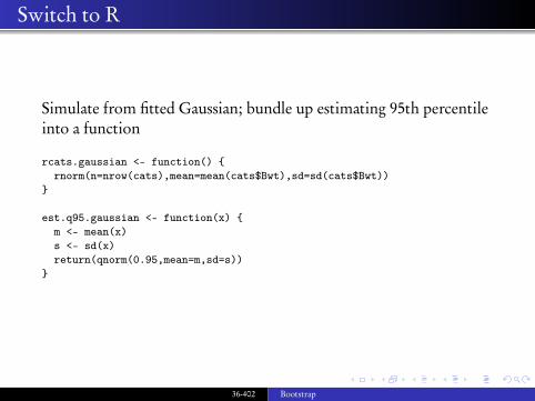
Simulate from fitted Gaussian; bundle up estimating 95th percentileinto a function

rcats.gaussian <- function() {rnorm(n=nrow(cats),mean=mean(cats$Bwt),sd=sd(cats$Bwt))

}

est.q95.gaussian <- function(x) {m <- mean(x)s <- sd(x)return(qnorm(0.95,mean=m,sd=s))

}

36-402 Bootstrap

Switch to R

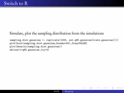
Simulate, plot the sampling distribution from the simulations

sampling.dist.gaussian <- replicate(1000, est.q95.gaussian(rcats.gaussian()))plot(hist(sampling.dist.gaussian,breaks=50),freq=FALSE)plot(density(sampling.dist.gaussian))abline(v=q95.gaussian,lty=2)

36-402 Bootstrap

Switch to R

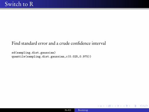
Find standard error and a crude confidence interval

sd(sampling.dist.gaussian)quantile(sampling.dist.gaussian,c(0.025,0.975))

36-402 Bootstrap

Improving on the Crude Confidence Interval

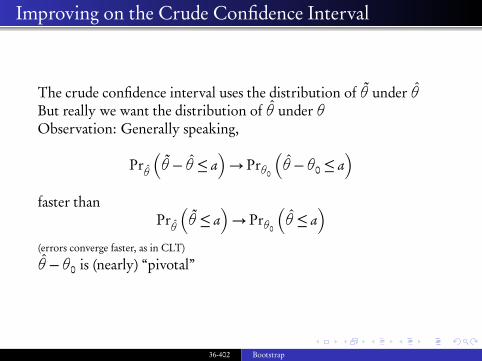
The crude confidence interval uses the distribution of θ under θBut really we want the distribution of θ under θObservation: Generally speaking,

Prθ

�

θ− θ≤ a�

→ Prθ0

�

θ−θ0 ≤ a�

faster thanPrθ

�

θ≤ a�

→ Prθ0

�

θ≤ a�

(errors converge faster, as in CLT)

θ−θ0 is (nearly) “pivotal”

36-402 Bootstrap

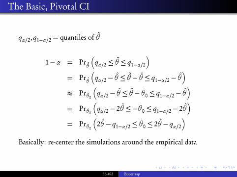
The Basic, Pivotal CI

qα/2,q1−α/2 = quantiles of θ

1−α = Prθ

�

qα/2 ≤ θ≤ q1−α/2

�

= Prθ

�

qα/2− θ≤ θ− θ≤ q1−α/2− θ�

≈ Prθ0

�

qα/2− θ≤ θ−θ0 ≤ q1−α/2− θ�

= Prθ0

�

qα/2− 2θ≤−θ0 ≤ q1−α/2− 2θ�

= Prθ0

�

2θ− q1−α/2 ≤ θ0 ≤ 2θ− qα/2�

Basically: re-center the simulations around the empirical data

36-402 Bootstrap

Switch to R

Find the basic CI

2*q95.gaussian - quantile(sampling.dist.gaussian,c(0.975,0.025))

36-402 Bootstrap

Model Checking

As always, if the model isn’t right, relying on the model is asking fortroubleHow good is the Gaussian as a model for the distribution of cats’weights?

36-402 Bootstrap

Switch to R

Compare histogram to fitted Gaussian density and to a smoothdensity estimate

plot(hist(cats$Bwt),freq=FALSE)curve(dnorm(x,mean=mean(cats$Bwt),sd=sd(cats$Bwt)),add=TRUE,col="purple")lines(density(cats$Bwt),lty=2)

36-402 Bootstrap

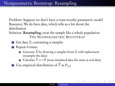
Nonparametric Bootstrap: Resampling

Problem: Suppose we don’t have a trust-worthy parametric modelResource; We do have data, which tells us a lot about thedistributionSolution: Resampling, treat the sample like a whole population

THE NONPARAMETRIC BOOTSTRAP

1 Get data X, containing n samples2 Repeat b times:

1 Generate X by drawing n samples from X with replacement(resample the data)

2 Calculate T = τX (treat simulated data the same as real data)3 Use empirical distribution of T as PT ,θ

36-402 Bootstrap

Is Moonshine Overweight, Take 2

Model-free estimate of the 95th percentile is the 95th percentile ofthe dataHow precise is that?

36-402 Bootstrap

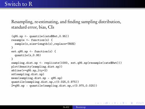
Switch to R

Resampling, re-estimating, and finding sampling distribution,standard error, bias, CIs

(q95.np <- quantile(cats$Bwt,0.95))resample <- function(x) {

sample(x,size=length(x),replace=TRUE)}est.q95.np <- function(x) {

quantile(x,0.95)}sampling.dist.np <- replicate(1000, est.q95.np(resample(cats$Bwt)))plot(density(sampling.dist.np))abline(v=q95.np,lty=2)sd(sampling.dist.np)mean(sampling.dist.np - q95.np)quantile(sampling.dist.np,c(0.025,0.975))2*q95.np - quantile(sampling.dist.np,c(0.975,0.025))

36-402 Bootstrap

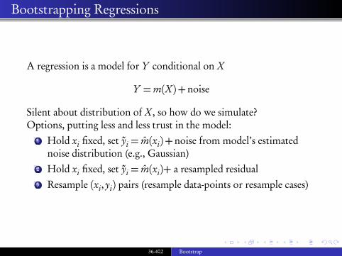
Bootstrapping Regressions

A regression is a model for Y conditional on X

Y =m(X)+noise

Silent about distribution of X, so how do we simulate?Options, putting less and less trust in the model:

1 Hold xi fixed, set yi = m(xi)+noise from model’s estimatednoise distribution (e.g., Gaussian)

2 Hold xi fixed, set yi = m(xi)+ a resampled residual3 Resample (xi,yi) pairs (resample data-points or resample cases)

36-402 Bootstrap

Cats’ Hearts

The cats data set has weights for cats’ hearts, as well as bodies

Much cuter than an actual photo of cats’ hearts

Source: http://yaleheartstudy.org/site/wp-content/uploads/2012/03/cat-heart1.jpg

How does heart weight relate to body weight?(Useful if Moonshine’s vet wants to know how much heart medicine to prescribe)

36-402 Bootstrap

Switch to R

Plot the data with the regression line

plot(Hwt~Bwt, data=cats, xlab="Body weight (kg)", ylab="Heart weight (g)")cats.lm <- lm(Hwt ~ Bwt, data=cats)abline(cats.lm)

36-402 Bootstrap

Switch to R

Coefficients and “official” confidence intervals:

coefficients(cats.lm)confint(cats.lm)

36-402 Bootstrap

Switch to R

The residuals don’t look very Gaussian:

plot(cats$Bwt,residuals(cats.lm))plot(density(residuals(cats.lm)))

36-402 Bootstrap

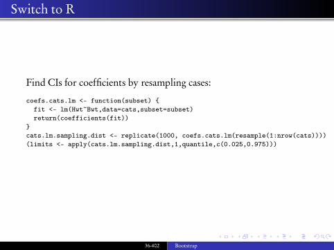
Switch to R

Find CIs for coefficients by resampling cases:

coefs.cats.lm <- function(subset) {fit <- lm(Hwt~Bwt,data=cats,subset=subset)return(coefficients(fit))

}cats.lm.sampling.dist <- replicate(1000, coefs.cats.lm(resample(1:nrow(cats))))(limits <- apply(cats.lm.sampling.dist,1,quantile,c(0.025,0.975)))

36-402 Bootstrap

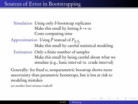
Sources of Error in Bootstrapping

Simulation Using only b bootstrap replicatesMake this small by letting b→∞Costs computing time

Approximation Using P instead of PX,θ0

Make this small by careful statistical modelingEstimation Only a finite number of samples

Make this small by being careful about what wesimulate (e.g., basic interval vs. crude interval)

Generally: for fixed n, nonparametric boostrap shows moreuncertainty than parametric bootstraps, but is less at risk tomodeling mistakesyet another bias-variance tradeoff

36-402 Bootstrap

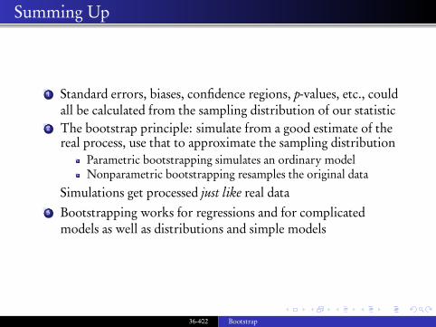
Summing Up

1 Standard errors, biases, confidence regions, p-values, etc., couldall be calculated from the sampling distribution of our statistic

2 The bootstrap principle: simulate from a good estimate of thereal process, use that to approximate the sampling distribution

Parametric bootstrapping simulates an ordinary modelNonparametric bootstrapping resamples the original data

Simulations get processed just like real data3 Bootstrapping works for regressions and for complicated

models as well as distributions and simple models

36-402 Bootstrap