nonlinear equations and optimization
TRANSCRIPT

Nonlinear Equations and Optimization

Motivation: Nonlinear Equations
So far we have mostly focused on linear phenomena
I Interpolation leads to a linear system Vb = y (monomials) orIb = y (Lagrange polynomials)
I Linear least-squares leads to the normal equationsATAb = AT y
I We saw examples of linear physical models (Ohm’s Law,Hooke’s Law, Leontief equations) =⇒ Ax = b
I F.D. discretization of a linear PDE leads to a linear algebraicsystem AU = F
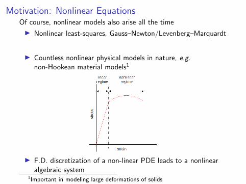
Motivation: Nonlinear EquationsOf course, nonlinear models also arise all the time
I Nonlinear least-squares, Gauss–Newton/Levenberg–Marquardt
I Countless nonlinear physical models in nature, e.g.non-Hookean material models1
I F.D. discretization of a non-linear PDE leads to a nonlinearalgebraic system
1Important in modeling large deformations of solids

Motivation: Nonlinear Equations
Another example is computation of Gauss quadraturepoints/weights
We know this is possible via roots of Legendre polynomials
But we could also try to solve the nonlinear system of equationsfor {(x1,w1), (x2,w2), . . . , (xn,wn)}

Motivation: Nonlinear Equations
e.g. for n = 2, we need to find points/weights such that allpolynomials of degree 3 are integrated exactly, hence
w1 + w2 =
∫ 1
−11dx = 2
w1x1 + w2x2 =
∫ 1
−1xdx = 0
w1x21 + w2x
22 =
∫ 1
−1x2dx = 2/3
w1x31 + w2x
32 =
∫ 1
−1x3dx = 0

Motivation: Nonlinear Equations
We usually write a nonlinear system of equations as
F (x) = 0,
where F : Rn → Rm
We implicity absorb the “right-hand side” into F and seek a rootof F
In this Unit we focus on the case m = n, m > n gives nonlinearleast-squares

Motivation: Nonlinear Equations
We are very familiar with scalar (m = 1) nonlinear equations
Simplest case is a quadratic equation
ax2 + bx + c = 0
We can write down a closed form solution, the quadratic formula
x =−b ±
√b2 − 4ac
2a

Motivation: Nonlinear Equations
In fact, there are also closed-form solutions for arbitrary cubic andquartic polynomials, due to Ferrari and Cardano (∼ 1540)
Important mathematical result is that there is no general formulafor solving fifth or higher order polynomial equations
Hence, even for the simplest possible case (polynomials), the onlyhope is to employ an iterative algorithm
An iterative method should converge in the limit n→∞, andideally yields an accurate approximation after few iterations

Motivation: Nonlinear Equations
There are many well-known iterative methods for nonlinearequations
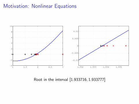
Probably the simplest is the bisection method for a scalar equationf (x) = 0, where f ∈ C [a, b]
Look for a root in the interval [a, b] by bisecting based on sign of f

Motivation: Nonlinear Equations
#!/usr/bin/python
from math import *
# Function to consider
def f(x):
return x*x-4*sin(x)
# Initial interval: assume f(a)<0 and f(b)>0
a=1
b=3
# Bisection search
while b-a>1e-8:
print a,b
c=0.5*(b+a)
if f(c)<0: a=c
else: b=c
print "# Root at",0.5*(a+b)
Motivation: Nonlinear Equations
1 1.5 2 2.5 3−4
−2
0
2
4
6
8
10
1.932 1.933 1.934 1.935
−0.01
−0.005
0
0.005
0.01
Root in the interval [1.933716, 1.933777]
Motivation: Nonlinear Equations
Bisection is a robust root-finding method in 1D, but it does notgeneralize easily to Rn for n > 1
Also, bisection is a crude method in the sense that it makes no useof magnitude of f , only sign(f )
We will look at mathematical basis of alternative methods whichgeneralize to Rn:
I Fixed-point iteration
I Newton’s method

Optimization

Motivation: Optimization
Another major topic in Scientific Computing is optimization
Very important in science, engineering, industry, finance,economics, logistics,...
Many engineering challenges can be formulated as optimizationproblems, e.g.:
I Design car body that maximizes downforce2
I Design a bridge with minimum weight
2A major goal in racing car design
Motivation: Optimization
Of course, in practice, it is more realistic to consider optimizationproblems with constraints, e.g.:
I Design car body that maximizes downforce, subject to aconstraint on drag
I Design a bridge with minimum weight, subject to a constrainton strength

Motivation: Optimization
Also, (constrained and unconstrained) optimization problems arisenaturally in science
Physics:
I many physical systems will naturally occupy a minimumenergy state
I if we can describe the energy of the system mathematically,then we can find minimum energy state via optimization
Motivation: Optimization
Biology:
I recent efforts in Scientific Computing have sought tounderstand biological phenomena quantitively via optimization
I computational optimization of, e.g. fish swimming or insectflight, can reproduce behavior observed in nature
I this jells with the idea that evolution has been “optimizing”organisms for millions of year

Motivation: Optimization
All these problems can be formulated as: Optimize (max. or min.)an objective function over a set of feasible choices, i.e.
Given an objective function f : Rn → R and a set S ⊂ Rn,we seek x∗ ∈ S such that f (x∗) ≤ f (x), ∀x ∈ S
(It suffices to consider only minimization, maximization isequivalent to minimizing −f )
S is the feasible set, usually defined by a set of equations and/orinequalities, which are the constraints
If S = Rn, then the problem is unconstrained

Motivation: Optimization
The standard way to write an optimization problem is
minx∈S
f (x) subject to g(x) = 0 and h(x) ≤ 0,
where f : Rn → R, g : Rn → Rm, h : Rn → Rp
Motivation: Optimization
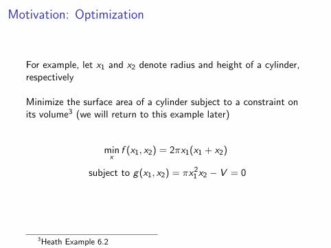
For example, let x1 and x2 denote radius and height of a cylinder,respectively
Minimize the surface area of a cylinder subject to a constraint onits volume3 (we will return to this example later)
minx
f (x1, x2) = 2πx1(x1 + x2)
subject to g(x1, x2) = πx21x2 − V = 0
3Heath Example 6.2

Motivation: Optimization
If f , g and h are all affine, then the optimization problem is calleda linear program
(Here the term “program” has nothing to do with computerprogramming; instead it refers to logistics/planning)
Affine if f (x) = Ax + b for a matrix A, i.e. linear plus a constant4
Linear programming mayalready be familiar
Just need to check f (x) onvertices of the feasible region
4Recall that “affine” is not the same as ”linear”, i.e.f (x + y) = Ax + Ay + b and f (x) + f (y) = Ax + Ay + 2b

Motivation: Optimization
If the objective function or any of the constraints are nonlinear thenwe have a nonlinear optimization problem or nonlinear program
We will consider several different approaches to nonlinearoptimization in this Unit
Optimization routines typically use local information about afunction to iteratively approach a local minimum

Motivation: Optimization
In some cases this easily gives a global minimum
−1 −0.5 0 0.5 10
0.5
1
1.5
2
2.5
3
Motivation: Optimization
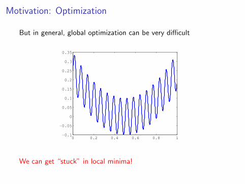
But in general, global optimization can be very difficult
0 0.2 0.4 0.6 0.8 1−0.1
−0.05
0
0.05
0.1
0.15
0.2
0.25
0.3
0.35
We can get “stuck” in local minima!

Motivation: Optimization
And can get much harder in higher spatial dimensions
0 0.2 0.4 0.6 0.8 10
0.1
0.2
0.3
0.4
0.5
0.6
0.7
0.8
0.9
1
−0.5
0
0.5
1
1.5
2
2.5

Motivation: Optimization
There are robust methods for finding local minimima, and this iswhat we focus on in AM205
Global optimization is very important in practice, but in generalthere is no way to guarantee that we will find a global minimum
Global optimization basically relies on heuristics:
I try several different starting guesses (“multistart” methods)
I simulated annealing
I genetic methods5
5Simulated annealing and genetic methods are covered in AM207

Root Finding: Scalar Case

Fixed-Point Iteration
Suppose we define an iteration
xk+1 = g(xk) (∗)
e.g. recall Heron’s Method from Assignment 0 for finding√a:
xk+1 =1
2
(xk +
a
xk
)This uses gheron(x) = 1
2 (x + a/x)

Fixed-Point Iteration
Suppose α is such that g(α) = α, then we call α a fixed point of g
For example, we see that√a is a fixed point of gheron since
gheron(√a) =
1
2
(√a + a/
√a)
=√a
A fixed-point iteration terminates once a fixed point is reached,since if g(xk) = xk then we get xk+1 = xk
Also, if xk+1 = g(xk) converges as k →∞, it must converge to afixed point: Let α ≡ limk→∞ xk , then6
α = limk→∞
xk+1 = limk→∞
g(xk) = g
(limk→∞
xk
)= g(α)
6Third equality requires g to be continuous

Fixed-Point Iteration
Hence, for example, we know if Heron’s method converges, it willconverge to
√a
It would be very helpful to know when we can guarantee that afixed-point iteration will converge
Recall that g satisfies a Lipschitz condition in an interval [a, b] if∃L ∈ R>0 such that
|g(x)− g(y)| ≤ L|x − y |, ∀x , y ∈ [a, b]
g is called a contraction if L < 1

Fixed-Point Iteration
Theorem: Suppose that g(α) = α and that g is a contractionon [α−A, α+A]. Suppose also that |x0−α| ≤ A. Then thefixed point iteration converges to α.
Proof:|xk − α| = |g(xk−1)− g(α)| ≤ L|xk−1 − α|,
which implies|xk − α| ≤ Lk |x0 − α|
and, since L < 1, |xk − α| → 0 as k →∞. (Note that|x0 − α| ≤ A implies that all iterates are in [α− A, α + A].) �
(This proof also shows that error decreases by factor of L eachiteration)

Fixed-Point Iteration
Recall that if g ∈ C 1[a, b], we can obtain a Lipschitz constantbased on g ′:
L = maxθ∈(a,b)
|g ′(θ)|
We now use this result to show that if |g ′(α)| < 1, then there is aneighborhood of α on which g is a contraction
This tells us that we can verify convergence of a fixed pointiteration by checking the gradient of g

Fixed-Point Iteration
By continuity of g ′ (and hence continuity of |g ′|), for any ε > 0∃δ > 0 such that for x ∈ (α− δ, α + δ):
| |g ′(x)| − |g ′(α)| | ≤ ε =⇒ maxx∈(α−δ,α+δ)
|g ′(x)| ≤ |g ′(α)|+ ε
Suppose |g ′(α)| < 1 and set ε = 12(1− |g ′(α)|), then there is a
neighborhood on which g is Lipschitz with L = 12(1 + |g ′(α)|)
Then L < 1 and hence g is a contraction in a neighborhood of α

Fixed-Point Iteration
Furthermore, as k →∞,
|xk+1 − α||xk − α|
=|g(xk)− g(α)||xk − α|
→ |g ′(α)|,
Hence, asymptotically, error decreases by a factor of |g ′(α)| eachiteration

Fixed-Point Iteration
We say that an iteration converges linearly if, for some µ ∈ (0, 1),
limk→∞
|xk+1 − α||xk − α|
= µ
An iteration converges superlinearly if
limk→∞
|xk+1 − α||xk − α|
= 0

Fixed-Point IterationWe can use these ideas to construct practical fixed-point iterationsfor solving f (x) = 0
e.g. suppose f (x) = ex − x − 2
0 0.5 1 1.5 2−1
−0.5
0
0.5
1
1.5
2
2.5
3
3.5
From the plot, it looks like there’s a root at x ≈ 1.15

Fixed-Point Iteration
f (x) = 0 is equivalent to x = log(x + 2), hence we seek a fixedpoint of the iteration
xk+1 = log(xk + 2), k = 0, 1, 2, . . .
Here g(x) ≡ log(x + 2), and g ′(x) = 1/(x + 2) < 1 for all x > −1,hence fixed point iteration will converge for x0 > −1
Hence we should get linear convergence with factor approx.g ′(1.15) = 1/(1.15 + 2) ≈ 0.32

Fixed-Point Iteration
An alternative fixed-point iteration is to set
xk+1 = exk − 2, k = 0, 1, 2, . . .
Therefore g(x) ≡ ex − 2, and g ′(x) = ex
Hence |g ′(α)| > 1, so we can’t guarantee convergence
(And, in fact, the iteration diverges...)

Fixed-Point Iteration
Python demo: Comparison of the two iterations
0 0.5 1 1.5 2−1
−0.5
0
0.5
1
1.5
2
2.5
3
3.5

Newton’s Method
Constructing fixed-point iterations can require some ingenuity
Need to rewrite f (x) = 0 in a form x = g(x), with appropriateproperties on g
To obtain a more generally applicable iterative method, let usconsider the following fixed-point iteration
xk+1 = xk − λ(xk)f (xk), k = 0, 1, 2, . . .
corresponding to g(x) = x − λ(x)f (x), for some function λ
A fixed point α of g yields a solution to f (α) = 0 (except possiblywhen λ(α) = 0), which is what we’re trying to achieve!

Newton’s Method
Recall that the asymptotic convergence rate is dictated by |g ′(α)|,so we’d like to have |g ′(α)| = 0 to get superlinear convergence
Suppose (as stated above) that f (α) = 0, then
g ′(α) = 1− λ′(α)f (α)− λ(α)f ′(α) = 1− λ(α)f ′(α)
Hence to satisfy g ′(α) = 0 we choose λ(x) ≡ 1/f ′(x) to getNewton’s method:
xk+1 = xk −f (xk)
f ′(xk), k = 0, 1, 2, . . .

Newton’s Method
Based on fixed-point iteration theory, Newton’s method isconvergent since |g ′(α)| = 0 < 1
However, we need a different argument to understand thesuperlinear convergence rate properly
To do this, we use a Taylor expansion for f (α) about f (xk):
0 = f (α) = f (xk) + (α− xk)f ′(xk) +(α− xk)2
2f ′′(θk)
for some θk ∈ (α, xk)

Newton’s Method
Dividing through by f ′(xk) gives(xk −
f (xk)
f ′(xk)
)− α =
f ′′(θk)
2f ′(xk)(xk − α)2,
or
xk+1 − α =f ′′(θk)
2f ′(xk)(xk − α)2,
Hence, roughly speaking, the error at iteration k + 1 is the squareof the error at each iteration k
This is referred to as quadratic convergence, which is very rapid!
Key point: Once again we need to be sufficiently close to α to getquadratic convergence (result relied on Taylor expansion near α)

Secant Method
An alternative to Newton’s method is to approximate f ′(xk) usingthe finite difference
f ′(xk) ≈ f (xk)− f (xk−1)
xk − xk−1
Substituting this into the iteration leads to the secant method
xk+1 = xk − f (xk)
(xk − xk−1
f (xk)− f (xk−1)
), k = 1, 2, 3, . . .
The main advantages of secant are:
I does not require us to determine f ′(x) analytically
I requires only one extra function evaluation, f (xk), periteration (Newton’s method also requires f ′(xk))

Secant Method
As one may expect, secant converges faster than a fixed-pointiteration, but slower than Newton’s method
In fact, it can be shown that for the secant method, we have
limk→∞
|xk+1 − α||xk − α|q
= µ
where µ is a positive constant and q ≈ 1.6
Python demo: Newton’s method versus secant method forf (x) = ex − x − 2 = 0

Multivariate Case
Systems of Nonlinear Equations
We now consider fixed-point iterations and Newton’s method forsystems of nonlinear equations
We suppose that F : Rn → Rn, n > 1, and we seek a root α ∈ Rn
such that F (α) = 0
In component form, this is equivalent to
F1(α) = 0
F2(α) = 0...
Fn(α) = 0

Fixed-Point Iteration
For a fixed-point iteration, we again seek to rewrite F (x) = 0 asx = G (x) to obtain:
xk+1 = G (xk)
The convergence proof is the same as in the scalar case, if wereplace | · | with ‖ · ‖
i.e. if ‖G (x)− G (y)‖ ≤ L‖x − y‖, then ‖xk − α‖ ≤ Lk‖x0 − α‖
Hence, as before, if G is a contraction it will converge to a fixedpoint α
Fixed-Point Iteration
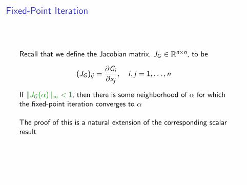
Recall that we define the Jacobian matrix, JG ∈ Rn×n, to be
(JG )ij =∂Gi
∂xj, i , j = 1, . . . , n
If ‖JG (α)‖∞ < 1, then there is some neighborhood of α for whichthe fixed-point iteration converges to α
The proof of this is a natural extension of the corresponding scalarresult

Fixed-Point Iteration
Once again, we can employ a fixed point iteration to solveF (x) = 0
e.g. consider
x21 + x22 − 1 = 0
5x21 + 21x22 − 9 = 0
This can be rearranged to x1 =√
1− x22 , x2 =√
(9− 5x21 )/21

Fixed-Point Iteration
Hence, we define
G1(x1, x2) ≡√
1− x22 , G2(x1, x2) ≡√
(9− 5x21 )/21
Python Example: This yields a convergent iterative method

Newton’s Method
As in the one-dimensional case, Newton’s method is generally moreuseful than a standard fixed-point iteration
The natural generalization of Newton’s method is
xk+1 = xk − JF (xk)−1F (xk), k = 0, 1, 2, . . .
Note that to put Newton’s method in the standard form for alinear system, we write
JF (xk)∆xk = −F (xk), k = 0, 1, 2, . . . ,
where ∆xk ≡ xk+1 − xk

Newton’s Method
Once again, if x0 is sufficiently close to α, then Newton’s methodconverges quadratically — we sketch the proof below
This result again relies on Taylor’s Theorem
Hence we first consider how to generalize the familiarone-dimensional Taylor’s Theorem to Rn
First, we consider the case for F : Rn → R

Multivariate Taylor Theorem
Let φ(s) ≡ F (x + sδ), then one-dimensional Taylor Theorem yields
φ(1) = φ(0) +k∑`=1
φ(`)(0)
`!+ φ(k+1)(η), η ∈ (0, 1),
Also, we have
φ(0) = F (x)
φ(1) = F (x + δ)
φ′(s) =∂F (x + sδ)
∂x1δ1 +
∂F (x + sδ)
∂x2δ2 + · · ·+ ∂F (x + sδ)
∂xnδn
φ′′(s) =∂2F (x + sδ)
∂x21
δ21 + · · ·+ ∂2F (x + sδ)
∂x1xnδ1δn + · · ·+
∂2F (x + sδ)
∂x1∂xnδ1δn + · · ·+ ∂2F (x + sδ)
∂x2n
δ2n
...
Multivariate Taylor Theorem
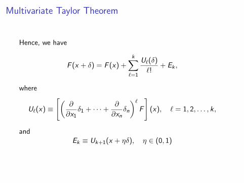
Hence, we have
F (x + δ) = F (x) +k∑`=1
U`(δ)
`!+ Ek ,
where
U`(x) ≡
[(∂
∂x1δ1 + · · ·+ ∂
∂xnδn
)`F
](x), ` = 1, 2, . . . , k ,
andEk ≡ Uk+1(x + ηδ), η ∈ (0, 1)

Multivariate Taylor Theorem
Let A be an upper bound on the abs. values of all derivatives oforder k + 1, then
|Ek | ≤1
(k + 1)!
∣∣∣(A, . . . ,A)T (‖δ‖k+1∞ , . . . , ‖δ‖k+1
∞ )∣∣∣
=1
(k + 1)!A‖δ‖k+1
∞
∣∣∣(1, . . . , 1)T (1, . . . , 1)∣∣∣
=nk+1
(k + 1)!A‖δ‖k+1
∞
where the last line follows from the fact that there are nk+1 termsin the inner product (i.e. there are nk+1 derivatives of order k + 1)

Multivariate Taylor Theorem
We shall only need an expansion up to first order terms for analysisof Newton’s method
From our expression above, we can write first order Taylorexpansion succinctly as:
F (x + δ) = F (x) +∇F (x)T δ + E1
Multivariate Taylor Theorem
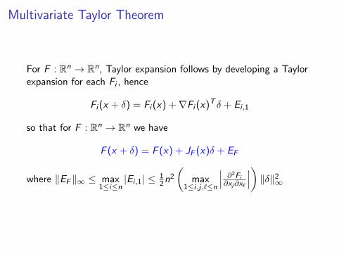
For F : Rn → Rn, Taylor expansion follows by developing a Taylorexpansion for each Fi , hence
Fi (x + δ) = Fi (x) +∇Fi (x)T δ + Ei ,1
so that for F : Rn → Rn we have
F (x + δ) = F (x) + JF (x)δ + EF
where ‖EF‖∞ ≤ max1≤i≤n
|Ei ,1| ≤ 12n
2
(max
1≤i ,j ,`≤n
∣∣∣ ∂2Fi∂xj∂x`
∣∣∣) ‖δ‖2∞
Newton’s Method
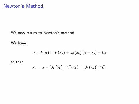
We now return to Newton’s method
We have
0 = F (α) = F (xk) + JF (xk) [α− xk ] + EF
so thatxk − α = [JF (xk)]−1F (xk) + [JF (xk)]−1EF

Newton’s Method
Also, the Newton iteration itself can be rewritten as
JF (xk) [xk+1 − α] = JF (xk) [xk − α]− F (xk)
Hence, we obtain:
xk+1 − α = [JF (xk)]−1EF ,
so that ‖xk+1 − α‖∞ ≤ const.‖xk − α‖2∞, i.e. quadraticconvergence!

Newton’s Method
Example: Newton’s method for the two-point Gauss quadraturerule
Recall the system of equations
F1(x1, x2,w1,w2) = w1 + w2 − 2 = 0
F2(x1, x2,w1,w2) = w1x1 + w2x2 = 0
F3(x1, x2,w1,w2) = w1x21 + w2x
22 − 2/3 = 0
F4(x1, x2,w1,w2) = w1x31 + w2x
32 = 0

Newton’s Method
We can solve this in Python using our own implementation ofNewton’s method
To do this, we require the Jacobian of this system:
JF (x1, x2,w1,w2) =
0 0 1 1w1 w2 x1 x2
2w1x1 2w2x2 x21 x223w1x
21 3w2x
22 x31 x32

Newton’s Method
Alternatively, we can use Python’s built-in fsolve function
Note that fsolve computes a finite difference approximation tothe Jacobian by default
(Or we can pass in an analytical Jacobian if we want)
Matlab has an equivalent fsolve function.

Newton’s Method
Python example: With either approach and with starting guessx0 = [−1, 1, 1, 1], we get
x k =
-0.577350269189626
0.577350269189626
1.000000000000000
1.000000000000000

Conditions for Optimality

Existence of Global Minimum
In order to guarantee existence and uniqueness of a global min. weneed to make assumptions about the objective function
e.g. if f is continuous on a closed7 and bounded set S ⊂ Rn thenit has global minimum in S
In one dimension, this says f achieves a minimum on the interval[a, b] ⊂ R
In general f does not achieve a minimum on (a, b), e.g. considerf (x) = x
(Though infx∈(a,b)
f (x), the largest lower bound of f on (a, b), is
well-defined)
7A set is closed if it contains its own boundary

Existence of Global Minimum
Another helpful concept for existence of global min. is coercivity
A continuous function f on an unbounded set S ⊂ Rn is coercive if
lim‖x‖→∞
f (x) = +∞
That is, f (x) must be large whenever ‖x‖ is large

Existence of Global Minimum
If f is coercive on a closed, unbounded8 set S , then f has a globalminimum in S
Proof: From the definition of coercivity, for any M ∈ R, ∃r > 0such that f (x) ≥ M for all x ∈ S where ‖x‖ ≥ r
Suppose that 0 ∈ S , and set M = f (0)
Let Y ≡ {x ∈ S : ‖x‖ ≥ r}, so that f (x) ≥ f (0) for all x ∈ Y
And we already know that f achieves a minimum (which is at mostf (0)) on the closed, bounded set {x ∈ S : ‖x‖ ≤ r}
Hence f achieves a minimum on S �
8e.g. S could be all of Rn, or a “closed strip” in Rn
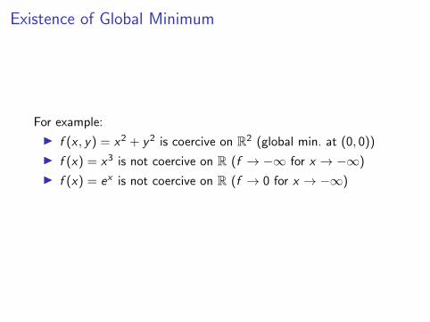
Existence of Global Minimum
For example:
I f (x , y) = x2 + y2 is coercive on R2 (global min. at (0, 0))
I f (x) = x3 is not coercive on R (f → −∞ for x → −∞)
I f (x) = ex is not coercive on R (f → 0 for x → −∞)

Convexity
An important concept for uniqueness is convexity
A set S ⊂ Rn is convex if it contains the line segment between anytwo of its points
That is, S is convex if for any x , y ∈ S , we have
{θx + (1− θ)y : θ ∈ [0, 1]} ⊂ S

Convexity
Similarly, we define convexity of a function f : S ⊂ Rn → R
f is convex if its graph along any line segment in S is on or belowthe chord connecting the function values
i.e. f is convex if for any x , y ∈ S and any θ ∈ (0, 1), we have
f (θx + (1− θ)y) ≤ θf (x) + (1− θ)f (y)
Also, iff (θx + (1− θ)y) < θf (x) + (1− θ)f (y)
then f is strictly convex

Convexity
−1 −0.5 0 0.5 10
0.5
1
1.5
2
2.5
3
Strictly convex

Convexity
0 0.2 0.4 0.6 0.8 1−0.1
−0.05
0
0.05
0.1
0.15
0.2
0.25
0.3
0.35
Non-convex

Convexity
0 0.2 0.4 0.6 0.8 10.1
0.15
0.2
0.25
0.3
0.35
0.4
0.45
0.5
Convex (not strictly convex)

Convexity
If f is a convex function on a convex set S , then any localminimum of f must be a global minimum9
Proof: Suppose x is a local minimum, i.e. f (x) ≤ f (y) fory ∈ B(x , ε) (where B(x , ε) ≡ {y ∈ S : ‖y − x‖ ≤ ε})
Suppose that x is not a global minimum, i.e. that there existsw ∈ S such that f (w) < f (x)
(Then we will show that this gives a contradiction)
9A global minimum is defined as a point z such that f (z) ≤ f (x) for allx ∈ S . Note that a global minimum may not be unique, e.g. if f (x) = − cos xthen 0 and 2π are both global minima.

Convexity
Proof (continued . . . ):
For θ ∈ [0, 1] we have f (θw + (1− θ)x) ≤ θf (w) + (1− θ)f (x)
Let σ ∈ (0, 1] be sufficiently small so that
z ≡ σw + (1− σ) x ∈ B(x , ε)
Then
f (z) ≤ σf (w) + (1− σ) f (x) < σf (x) + (1− σ) f (x) = f (x),
i.e. f (z) < f (x), which contradicts that f (x) is a local minimum!
Hence we cannot have w ∈ S such that f (w) < f (x) �
Convexity
Note that convexity does not guarantee uniqueness of globalminimum
e.g. a convex function can clearly have a “horizontal” section (seeearlier plot)
If f is a strictly convex function on a convex set S , then a localminimum of f is the unique global minimum
Optimization of convex functions over convex sets is called convexoptimization, which is an important subfield of optimization

Optimality Conditions
We have discussed existence and uniqueness of minima, buthaven’t considered how to find a minimum
The familiar optimization idea from calculus in one dimension is:set derivative to zero, check the sign of the second derivative
This can be generalized to Rn

Optimality Conditions
If f : Rn → R is differentiable, then the gradient vector∇f : Rn → Rn is
∇f (x) ≡
∂f (x)∂x1∂f (x)∂x2...
∂f (x)∂xn
The importance of the gradient is that ∇f points “uphill,” i.e.towards points with larger values than f (x)
And similarly −∇f points “downhill”
Optimality Conditions
This follows from Taylor’s theorem for f : Rn → R
Recall that
f (x + δ) = f (x) +∇f (x)T δ + H.O.T.
Let δ ≡ −ε∇f (x) for ε > 0 and suppose that ∇f (x) 6= 0, then:
f (x − ε∇f (x)) ≈ f (x)− ε∇f (x)T∇f (x) < f (x)
Also, we see from Cauchy–Schwarz that −∇f (x) is the steepestdescent direction

Optimality Conditions
Similarly, we see that a necessary condition for a local minimum atx∗ ∈ S is that ∇f (x∗) = 0
In this case there is no “downhill direction” at x∗
The condition ∇f (x∗) = 0 is called a first-order necessarycondition for optimality, since it only involves first derivatives

Optimality Conditions
x∗ ∈ S that satisfies the first-order optimality condition is called acritical point of f
But of course a critical point can be a local min., local max., orsaddle point
(Recall that a saddle point is where some directions are “downhill”and others are “uphill”, e.g. (x , y) = (0, 0) for f (x , y) = x2 − y2)
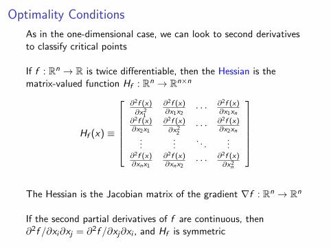
Optimality Conditions
As in the one-dimensional case, we can look to second derivativesto classify critical points
If f : Rn → R is twice differentiable, then the Hessian is thematrix-valued function Hf : Rn → Rn×n
Hf (x) ≡
∂2f (x)∂x21
∂2f (x)∂x1x2
· · · ∂2f (x)∂x1xn
∂2f (x)∂x2x1
∂2f (x)∂x22
· · · ∂2f (x)∂x2xn
......
. . ....
∂2f (x)∂xnx1
∂2f (x)∂xnx2
· · · ∂2f (x)∂x2n
The Hessian is the Jacobian matrix of the gradient ∇f : Rn → Rn
If the second partial derivatives of f are continuous, then∂2f /∂xi∂xj = ∂2f /∂xj∂xi , and Hf is symmetric
Optimality Conditions
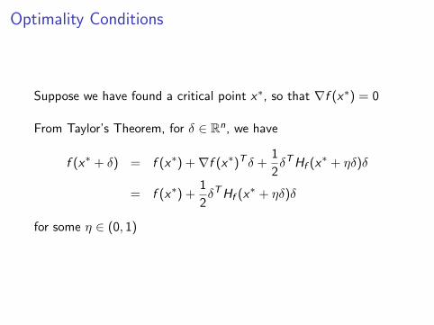
Suppose we have found a critical point x∗, so that ∇f (x∗) = 0
From Taylor’s Theorem, for δ ∈ Rn, we have
f (x∗ + δ) = f (x∗) +∇f (x∗)T δ +1
2δTHf (x∗ + ηδ)δ
= f (x∗) +1
2δTHf (x∗ + ηδ)δ
for some η ∈ (0, 1)

Optimality Conditions
Recall positive definiteness: A is positive definite if xTAx > 0
Suppose Hf (x∗) is positive definite
Then (by continuity) Hf (x∗ + ηδ) is also positive definite for ‖δ‖sufficiently small, so that: δTHf (x∗ + ηδ)δ > 0
Hence, we have f (x∗ + δ) > f (x∗) for ‖δ‖ sufficiently small, i.e.f (x∗) is a local minimum
Hence, in general, positive definiteness of Hf at a critical point x∗
is a second-order sufficient condition for a local minimum

Optimality Conditions
A matrix can also be negative definite: xTAx < 0 for all x 6= 0
Or indefinite: There exists x , y such that xTAx < 0 < yTAy
Then we can classify critical points as follows:
I Hf (x∗) positive definite =⇒ x∗ is a local minimum
I Hf (x∗) negative definite =⇒ x∗ is a local maximum
I Hf (x∗) indefinite =⇒ x∗ is a saddle point
Optimality Conditions
Also, positive definiteness of the Hessian is closely related toconvexity of f
If Hf (x) is positive definite, then f is convex on some convexneighborhood of x
If Hf (x) is positive definite for all x ∈ S , where S is a convex set,then f is convex on S
Question: How do we test for positive definiteness?

Optimality Conditions
Answer: A is positive (resp. negative) definite if and only if alleigenvalues of A are positive (resp. negative)10
Also, a matrix with positive and negative eigenvalues is indefinite
Hence we can compute all the eigenvalues of A and check theirsigns
10This is related to the Rayleigh quotient, see Unit V

Heath Example 6.5
Consider
f (x) = 2x31 + 3x21 + 12x1x2 + 3x22 − 6x2 + 6
Then
∇f (x) =
[6x21 + 6x1 + 12x2
12x1 + 6x2 − 6
]
We set ∇f (x) = 0 to find critical points11 [1,−1]T and [2,−3]T
11In general solving ∇f (x) = 0 requires an iterative method

Heath Example 6.5, continued . . .
The Hessian is
Hf (x) =
[12x1 + 6 12
12 6
]and hence
Hf (1,−1) =
[18 1212 6
], which has eigenvalues 25.4,−1.4
Hf (2,−3) =
[30 1212 6
], which has eigenvalues 35.0, 1.0
Hence [2,−3]T is a local min. whereas [1,−1]T is a saddle point

Optimality Conditions: Equality Constrained Case
So far we have ignored constraints
Let us now consider equality constrained optimization
minx∈Rn
f (x) subject to g(x) = 0,
where f : Rn → R and g : Rn → Rm, with m ≤ n
Since g maps to Rm, we have m constraints
This situation is treated with Lagrange mutlipliers
Optimality Conditions: Equality Constrained Case
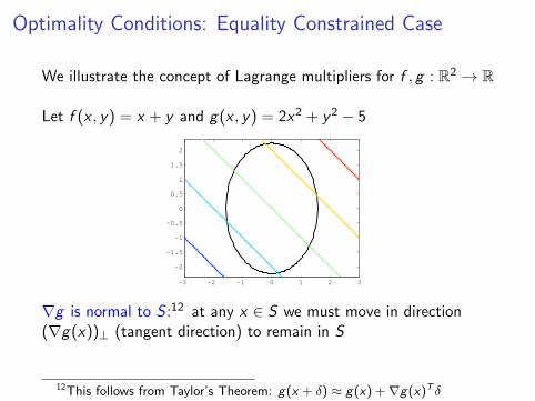
We illustrate the concept of Lagrange multipliers for f , g : R2 → R
Let f (x , y) = x + y and g(x , y) = 2x2 + y2 − 5
−3 −2 −1 0 1 2 3
−2
−1.5
−1
−0.5
0
0.5
1
1.5
2
∇g is normal to S :12 at any x ∈ S we must move in direction(∇g(x))⊥ (tangent direction) to remain in S
12This follows from Taylor’s Theorem: g(x + δ) ≈ g(x) +∇g(x)T δ
Optimality Conditions: Equality Constrained Case
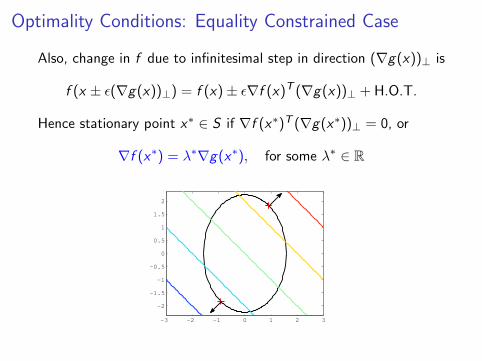
Also, change in f due to infinitesimal step in direction (∇g(x))⊥ is
f (x ± ε(∇g(x))⊥) = f (x)± ε∇f (x)T (∇g(x))⊥ + H.O.T.
Hence stationary point x∗ ∈ S if ∇f (x∗)T (∇g(x∗))⊥ = 0, or
∇f (x∗) = λ∗∇g(x∗), for some λ∗ ∈ R
−3 −2 −1 0 1 2 3
−2
−1.5
−1
−0.5
0
0.5
1
1.5
2
Optimality Conditions: Equality Constrained Case
This shows that for a stationary point with m = 1 constraints, ∇fcannot have any component in the “tangent direction” to S
Now, consider the case with m > 1 equality constraints
Then g : Rn → Rm and we now have a set of constraint gradientvectors, ∇gi , i = 1, . . . ,m
Then we have S = {x ∈ Rn : gi (x) = 0, i = 1, . . . ,m}
Any “tangent direction” at x ∈ S must be orthogonal to allgradient vectors {∇gi (x), i = 1, . . . ,m} to remain in S
Optimality Conditions: Equality Constrained Case
Let T (x) ≡ {v ∈ Rn : ∇gi (x)T v = 0, i = 1, 2, . . . ,m} denote theorthogonal complement of {∇gi (x), i = 1, . . . ,m}
Then, for δ ∈ T (x) and ε ∈ R>0, εδ is a step in a “tangentdirection” of S at x
Since we have
f (x∗ + εδ) = f (x∗) + ε∇f (x∗)T δ + H.O.T.
it follows that for a stationary point we need ∇f (x∗)T δ = 0 for allδ ∈ T (x∗)
Optimality Conditions: Equality Constrained Case
Hence, we require that at a stationary point x∗ ∈ S we have
∇f (x∗) ∈ span{∇gi (x∗), i = 1, . . . ,m}
This can be written succinctly as a linear system
∇f (x∗) = (Jg (x∗))Tλ∗
for some λ∗ ∈ Rm, where (Jg (x∗))T ∈ Rn×m
This follows because the columns of (Jg (x∗))T are the vectors{∇gi (x∗), i = 1, . . . ,m}

Optimality Conditions: Equality Constrained Case
We can write equality constrained optimization problems moresuccinctly by introducing the Lagrangian function, L : Rn+m → R,
L(x , λ) ≡ f (x) + λTg(x)
= f (x) + λ1g1(x) + · · ·+ λmgm(x)
Then we have,
∂L(x ,λ)∂xi
= ∂f (x)∂xi
+ λ1∂g1(x)∂xi
+ · · ·+ λn∂gn(x)∂xi
, i = 1, . . . , n
∂L(x ,λ)∂λi
= gi (x), i = 1, . . . ,m

Optimality Conditions: Equality Constrained Case
Hence
∇L(x , λ) =
[∇xL(x , λ)∇λL(x , λ)
]=
[∇f (x) + Jg (x)Tλ
g(x)
],
so that the first order necessary condition for optimality for theconstrained problem can be written as a nonlinear system:13
∇L(x , λ) =
[∇f (x) + Jg (x)Tλ
g(x)
]= 0
(As before, stationary points can be classified by considering theHessian, though we will not consider this here . . . )
13n + m variables, n + m equations
Optimality Conditions: Equality Constrained Case
See Lecture: Constrained optimization of cylinder surface area

Optimality Conditions: Equality Constrained Case
As another example of equality constrained optimization, recall ourunderdetermined linear least squares problem from I.3
minb∈Rn
f (b) subject to g(b) = 0,
where f (b) ≡ bTb, g(b) ≡ Ab − y and A ∈ Rm×n with m < n

Optimality Conditions: Equality Constrained Case
Introducing Lagrange multipliers gives
L(b, λ) ≡ bTb + λT (Ab − y)
where b ∈ Rn and λ ∈ Rm
Hence ∇L(b, λ) = 0 implies[∇f (b) + Jg (b)Tλ
g(b)
]=
[2b + ATλAb − y
]= 0 ∈ Rn+m
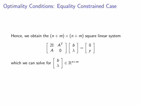
Optimality Conditions: Equality Constrained Case
Hence, we obtain the (n + m)× (n + m) square linear system[2I AT
A 0
] [bλ
]=
[0y
]
which we can solve for
[bλ
]∈ Rn+m

Optimality Conditions: Equality Constrained Case
We have b = −12A
Tλ from the first “block row”
Subsituting into Ab = y (the second “block row”) yieldsλ = −2(AAT )−1y
And hence
b = −1
2ATλ = AT (AAT )−1y
which was the solution we introduced (but didn’t derive) in I.3

Optimality Conditions: Inequality Constrained Case
Similar Lagrange multiplier methods can be developed for the moredifficult case of inequality constrained optimization
Steepest Descent
We first consider the simpler case of unconstrained optimization(as opposed to constrained optimization)
Perhaps the simplest method for unconstrained optimization issteepest descent
Key idea: The negative gradient −∇f (x) points in the “steepestdownhill” direction for f at x
Hence an iterative method for minimizing f is obtained byfollowing −∇f (xk) at each step
Question: How far should we go in the direction of −∇f (xk)?

Steepest Descent
We can try to find the best step size via a subsidiary (and easier!)optimization problem
For a direction s ∈ Rn, let φ : R→ R be given by
φ(η) = f (x + ηs)
Then minimizing f along s corresponds to minimizing theone-dimensional function φ
This process of minimizing f along a line is called a line search14
14The line search can itself be performed via Newton’s method, as describedfor f : Rn → R shortly, or via a built-in function
Steepest Descent
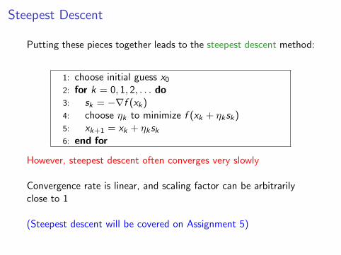
Putting these pieces together leads to the steepest descent method:
1: choose initial guess x02: for k = 0, 1, 2, . . . do3: sk = −∇f (xk)4: choose ηk to minimize f (xk + ηksk)5: xk+1 = xk + ηksk6: end for
However, steepest descent often converges very slowly
Convergence rate is linear, and scaling factor can be arbitrarilyclose to 1
(Steepest descent will be covered on Assignment 5)

Newton’s Method
We can get faster convergence by using more information about f
Note that ∇f (x∗) = 0 is a system of nonlinear equations, hence wecan solve it with quadratic convergence via Newton’s method15
The Jacobian matrix of ∇f (x) is Hf (x) and hence Newton’smethod for unconstrained optimization is:
1: choose initial guess x02: for k = 0, 1, 2, . . . do3: solve Hf (xk)sk = −∇f (xk)4: xk+1 = xk + sk5: end for
15Note that in its simplest form this algorithm searches for stationary points,not necessarily minima
Newton’s Method
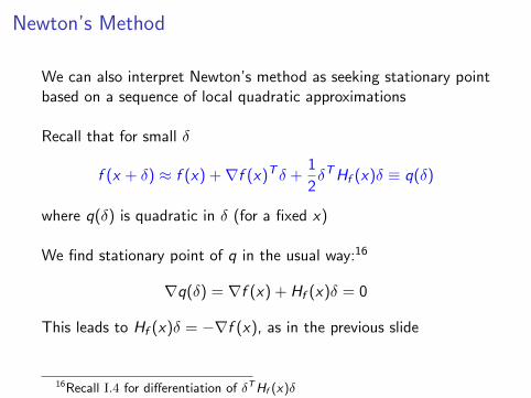
We can also interpret Newton’s method as seeking stationary pointbased on a sequence of local quadratic approximations
Recall that for small δ
f (x + δ) ≈ f (x) +∇f (x)T δ +1
2δTHf (x)δ ≡ q(δ)
where q(δ) is quadratic in δ (for a fixed x)
We find stationary point of q in the usual way:16
∇q(δ) = ∇f (x) + Hf (x)δ = 0
This leads to Hf (x)δ = −∇f (x), as in the previous slide
16Recall I.4 for differentiation of δTHf (x)δ

Newton’s Method
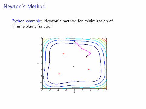
Python example: Newton’s method for minimization ofHimmelblau’s function
f (x , y) = (x2 + y − 11)2 + (x + y2 − 7)2
Local maximum of 181.617 at (−0.270845,−0.923039)
Four local minima, each of 0, at
(3, 2), (−2.805, 3.131), (−3.779,−3.283), (3.584,−1.841)
Newton’s Method
Python example: Newton’s method for minimization ofHimmelblau’s function
x
y
−8 −6 −4 −2 0 2 4 6 8−8
−6
−4
−2
0
2
4
6
8
Newton’s Method: Robustness
Newton’s method generally converges much faster than steepestdescent
However, Newton’s method can be unreliable far away from asolution
To improve robustness during early iterations it is common toperform a line search in the Newton-step-direction
Also line search can ensure we don’t approach a local max. as canhappen with raw Newton method
The line search modifies the Newton step size, hence often referredto as a damped Newton method
Newton’s Method: Robustness
Another way to improve robustness is with trust region methods
At each iteration k , a “trust radius” Rk is computed
This determines a region surrounding xk on which we “trust” ourquadratic approx.
We require ‖xk+1 − xk‖ ≤ Rk , hence constrained optimizationproblem (with quadratic objective function) at each step

Newton’s Method: Robustness
Size of Rk+1 is based on comparing actual change,f (xk+1)− f (xk), to change predicted by the quadratic model
If quadratic model is accurate, we expand the trust radius,otherwise we contract it
When close to a minimum, Rk should be large enough to allow fullNewton steps =⇒ eventual quadratic convergence

Quasi-Newton Methods
Newton’s method is effective for optimization, but it can beunreliable, expensive, and complicated
I Unreliable: Only converges when sufficiently close to aminimum
I Expensive: The Hessian Hf is dense in general, hence veryexpensive if n is large
I Complicated: Can be impractical or laborious to derive theHessian
Hence there has been much interest in so-called quasi-Newtonmethods, which do not require the Hessian

Quasi-Newton Methods
General form of quasi-Newton methods:
xk+1 = xk − αkB−1k ∇f (xk)
where αk is a line search parameter and Bk is some approximationto the Hessian
Quasi-Newton methods generally lose quadratic convergence ofNewton’s method, but often superlinear convergence is achieved
We now consider some specific quasi-Newton methods

BFGS
The Broyden–Fletcher–Goldfarb–Shanno (BFGS) method is one ofthe most popular quasi-Newton methods:
1: choose initial guess x02: choose B0, initial Hessian guess, e.g. B0 = I3: for k = 0, 1, 2, . . . do4: solve Bksk = −∇f (xk)5: xk+1 = xk + sk6: yk = ∇f (xk+1)−∇f (xk)7: Bk+1 = Bk + ∆Bk
8: end for
where
∆Bk ≡yky
Tk
yTk sk−
BksksTk Bk
sTk Bksk

BFGS
See lecture: derivation of the Broyden root-finding algorithm
See lecture: derivation of the BFGS algorithm
Basic idea is that Bk accumulates second derivative information onsuccessive iterations, eventually approximates Hf well
BFGS
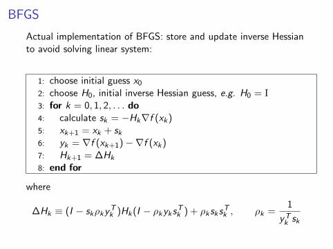
Actual implementation of BFGS: store and update inverse Hessianto avoid solving linear system:
1: choose initial guess x02: choose H0, initial inverse Hessian guess, e.g. H0 = I3: for k = 0, 1, 2, . . . do4: calculate sk = −Hk∇f (xk)5: xk+1 = xk + sk6: yk = ∇f (xk+1)−∇f (xk)7: Hk+1 = ∆Hk
8: end for
where
∆Hk ≡ (I − skρkyTk )Hk(I − ρkyksTk ) + ρksks
Tk , ρk =
1
yTk sk

BFGS
BFGS is implemented as the fmin bfgs function inscipy.optimize
Also, BFGS (+ trust region) is implemented in Matlab’s fminuncfunction, e.g.
x0 = [5;5];
options = optimset(’GradObj’,’on’);
[x,fval,exitflag,output] = ...
fminunc(@himmelblau_function,x0,options);
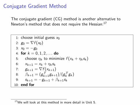
Conjugate Gradient Method
The conjugate gradient (CG) method is another alternative toNewton’s method that does not require the Hessian:17
1: choose initial guess x02: g0 = ∇f (x0)3: x0 = −g04: for k = 0, 1, 2, . . . do5: choose ηk to minimize f (xk + ηksk)6: xk+1 = xk + ηksk7: gk+1 = ∇f (xk+1)8: βk+1 = (gT
k+1gk+1)/(gTk gk)
9: sk+1 = −gk+1 + βk+1sk10: end for
17We will look at this method in more detail in Unit 5.

Constrained Optimization

Equality Constrained Optimization
We now consider equality constrained minimization:
minx∈Rn
f (x) subject to g(x) = 0,
where f : Rn → R and g : Rn → Rm
With the Lagrangian L(x , λ) = f (x) + λTg(x), we recall from thatnecessary condition for optimality is
∇L(x , λ) =
[∇f (x) + JTg (x)λ
g(x)
]= 0
Once again, this is a nonlinear system of equations that can besolved via Newton’s method

Sequential Quadratic Programming
To derive the Jacobian of this system, we write
∇L(x , λ) =
[∇f (x) +
∑mk=1 λk∇gk(x)
g(x)
]∈ Rn+m
Then we need to differentiate wrt to x ∈ Rn and λ ∈ Rm
For i = 1, . . . , n, we have
(∇L(x , λ))i =∂f (x)
∂xi+
m∑k=1
λk∂gk(x)
∂xi
Differentiating wrt xj , for i , j = 1, . . . , n, gives
∂
∂xj(∇L(x , λ))i =
∂2f (x)
∂xi∂xj+
m∑k=1
λk∂2gk(x)
∂xi∂xj

Sequential Quadratic Programming
Hence the top-left n × n block of the Jacobian of ∇L(x , λ) is
B(x , λ) ≡ Hf (x) +m∑
k=1
λkHgk (x) ∈ Rn×n
Differentiating (∇L(x , λ))i wrt λj , for i = 1, . . . , n, j = 1, . . . ,m,gives
∂
∂λj(∇L(x , λ))i =
∂gj(x)
∂xi
Hence the top-right n ×m block of the Jacobian of ∇L(x , λ) is
Jg (x)T ∈ Rn×m

Sequential Quadratic Programming
For i = n + 1, . . . , n + m, we have
(∇L(x , λ))i = gi (x)
Differentiating (∇L(x , λ))i wrt xj , for i = n + 1, . . . , n + m,j = 1, . . . , n, gives
∂
∂xj(∇L(x , λ))i =
∂gi (x)
∂xj
Hence the bottom-left m × n block of the Jacobian of ∇L(x , λ) is
Jg (x) ∈ Rm×n
. . . and the final m ×m bottom right block is just zero(differentiation of gi (x) w.r.t. λj)
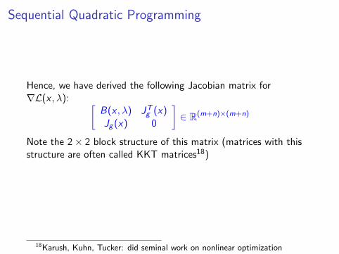
Sequential Quadratic Programming
Hence, we have derived the following Jacobian matrix for∇L(x , λ): [
B(x , λ) JTg (x)Jg (x) 0
]∈ R(m+n)×(m+n)
Note the 2× 2 block structure of this matrix (matrices with thisstructure are often called KKT matrices18)
18Karush, Kuhn, Tucker: did seminal work on nonlinear optimization

Sequential Quadratic Programming
Therefore, Newton’s method for ∇L(x , λ) = 0 is:[B(xk , λk) JTg (xk)Jg (xk) 0
] [skδk
]= −
[∇f (xk) + JTg (xk)λk
g(xk)
]for k = 0, 1, 2, . . .
Here (sk , δk) ∈ Rn+m is the kth Newton step

Sequential Quadratic Programming
Now, consider the constrained minimization problem, where(xk , λk) is our Newton iterate at step k :
mins
{1
2sTB(xk , λk)s + sT (∇f (xk) + JTg (xk)λk)
}subject to Jg (xk)s + g(xk) = 0
The objective function is quadratic in s (here xk , λk are constants)
This minimization problem has Lagrangian
Lk(s, δ) ≡ 1
2sTB(xk , λk)s + sT (∇f (xk) + JTg (xk)λk)
+ δT (Jg (xk)s + g(xk))
Sequential Quadratic Programming
Then solving ∇Lk(s, δ) = 0 (i.e. first-order necessary conditions)gives a linear system, which is the same as the kth Newton step
Hence at each step of Newton’s method, we exactly solve aminimization problem (quadratic objective fn., linear constraints)
An optimization problem of this type is called a quadratic program
This motivates the name for applying Newton’s method toL(x , λ) = 0: Sequential Quadratic Programming (SQP)

Sequential Quadratic Programming
SQP is an important method, and there are many issues to beconsidered to obtain an efficient and reliable implementation:
I Efficient solution of the linear systems at each Newtoniteration — matrix block structure can be exploited
I Quasi-Newton approximations to the Hessian (as in theunconstrained case)
I Trust region, line search etc to improve robustness
I Treatment of constraints (equality and inequality) during theiterative process
I Selection of good starting guess for λ

Penalty Methods
Another computational strategy for constrained optimization is toemploy penalty methods
This converts a constrained problem into an unconstrained problem
Key idea: Introduce a new objective function which is a weightedsum of objective function and constraint

Penalty Methods
Given the minimization problem
minx
f (x) subject to g(x) = 0
we can consider the related unconstrained problem
minxφρ(x) = f (x) +
1
2ρg(x)Tg(x) (∗∗)
Let x∗ and x∗ρ denote the solution of (∗) and (∗∗), respectively
Under appropriate conditions, it can be shown that
limρ→∞
x∗ρ = x∗

Penalty Methods
In practice, we can solve the unconstrained problem for a largevalue of ρ to get a good approximation of x∗
Another strategy is to solve for a sequence of penalty parameters,ρk , where x∗ρk serves as a starting guess for x∗ρk+1
Note that the major drawback of penalty methods is that a largefactor ρ will increase the condition number of the Hessian Hφρ
On the other hand, penalty methods can be convenient, primarilydue to their simplicity

Linear Programming

Linear Programming
As we mentioned earlier, the optimization problem
minx∈Rn
f (x) subject to g(x) = 0 and h(x) ≤ 0, (∗)
with f , g , h affine, is called a linear program
The feasible region is a convex polyhedron19
Since the objective function maps out a hyperplane, its globalminimum must occur at a vertex of the feasible region
19Polyhedron: a solid with flat sides, straight edges

Linear Programming
This can be seen most easily with a picture (in R2)

Linear Programming
The standard approach for solving linear programs is conceptuallysimple: examine a sequence of the vertices to find the minimum
This is called the simplex method
Despite its conceptual simplicity, it is non-trivial to develop anefficient implementation of this algorithm
We will not discuss the implementation details of the simplexmethod...

Linear Programming
In the worst case, the computational work required for the simplexmethod grows exponentially with the size of the problem
But this worst-case behavior is extremely rare; in practice simplexis very efficient (computational work typically grows linearly)
Newer methods, called interior point methods, have beendeveloped that are polynomial in the worst case
Nevertheless, simplex is still the standard approach since it is moreefficient than interior point for most problems
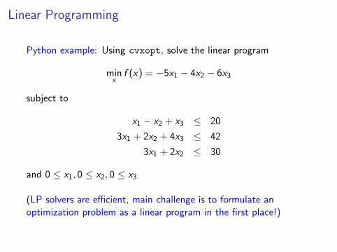
Linear Programming
Python example: Using cvxopt, solve the linear program
minx
f (x) = −5x1 − 4x2 − 6x3
subject to
x1 − x2 + x3 ≤ 20
3x1 + 2x2 + 4x3 ≤ 42
3x1 + 2x2 ≤ 30
and 0 ≤ x1, 0 ≤ x2, 0 ≤ x3
(LP solvers are efficient, main challenge is to formulate anoptimization problem as a linear program in the first place!)

PDE Constrained Optimization
Here we will focus on the form we introduced first:
minp∈RnG(p)
Optimization methods usually need some derivative information,such as using finite differences to approximate ∇G(p)

PDE Constrained Optimization
But using finite differences can be expensive, especially if we havemany parameters:
∂G(p)
∂pi≈ G(p + hei )− G(p)
h,
hence we need n + 1 evaluations of G to approximate ∇G(p)!
We saw from the Himmelblau example that supplying the gradient∇G(p) cuts down on the number of function evaluations required
The extra function calls due to F.D. isn’t a big deal forHimmelblau’s function, each evaluation is very cheap
But in PDE constrained optimization, each p → G(p) requires afull PDE solve!
PDE Constrained Optimization
Hence for PDE constrained optimization with many parameters, itis important to be able to compute the gradient more efficiently
There are two main approaches:
I the direct method
I the adjoint method
The direct method is simpler, but the adjoint method is muchmore efficient if we have many parameters

PDE Output Derivatives
Consider the ODE BVP
−u′′(x ; p) + r(x ; p)u(x ; p) = f (x), u(a) = u(b) = 0
which we will refer to as the primal equation
Here p ∈ Rn is the parameter vector, and r : R× Rn → R
We define an output functional based on an integral
g(u) ≡∫ b
aσ(x)u(x)dx ,
for some function σ; then G(p) ≡ g(u(p)) ∈ R

The Direct Method
We observe that
∂G(p)
∂pi=
∫ b
aσ(x)
∂u
∂pidx
hence if we can compute ∂u∂pi
, i = 1, 2, . . . , n, then we can obtainthe gradient
Assuming sufficient smoothness, we can “differentiate the ODEBVP” wrt pi to obtain,
− ∂u∂pi
′′(x ; p) + r(x ; p)
∂u
∂pi(x ; p) = − ∂r
∂piu(x ; p)
for i = 1, 2, . . . , n

The Direct Method
Once we compute each ∂u∂pi
we can then evaluate ∇G(p) byevaluating a sequence of n integrals
However, this is not much better than using finite differences: Westill need to solve n separate ODE BVPs
(Though only the right-hand side changes, so could LU factorizethe system matrix once and back/forward sub. for each i)

Adjoint-Based Method
However, a more efficient approach when n is large is the adjointmethod
We introduce the adjoint equation:
−z ′′(x ; p) + r(x ; p)z(x ; p) = σ(x), z(a) = z(b) = 0
Adjoint-Based Method
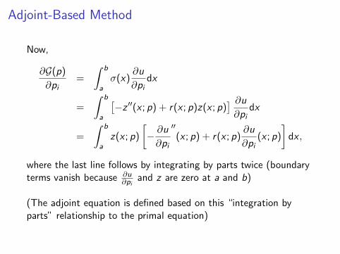
Now,
∂G(p)
∂pi=
∫ b
aσ(x)
∂u
∂pidx
=
∫ b
a
[−z ′′(x ; p) + r(x ; p)z(x ; p)
] ∂u∂pi
dx
=
∫ b
az(x ; p)
[− ∂u∂pi
′′(x ; p) + r(x ; p)
∂u
∂pi(x ; p)
]dx ,
where the last line follows by integrating by parts twice (boundaryterms vanish because ∂u
∂piand z are zero at a and b)
(The adjoint equation is defined based on this “integration byparts” relationship to the primal equation)

Adjoint-Based Method
Also, recalling the derivative of the primal problem with respect topi :
− ∂u∂pi
′′(x ; p) + r(x ; p)
∂u
∂pi(x ; p) = − ∂r
∂piu(x ; p),
we get∂G(p)
∂pi= −
∫ b
a
∂r
∂piz(x ; p)u(x ; p)dx
Therefore, we only need to solve two differential equations (primaland adjoint) to obtain ∇G(p)! Each component of the gradientrequires a single integration.
For more complicated PDEs the adjoint formulation is morecomplicated but the basic ideas stay the same