nonlinear control - pudn.comread.pudn.com/downloads780/ebook/3088175/nonlinear... · from nonlinear...
TRANSCRIPT


Nonlinear Control

This page intentionally left blank

Nonlinear Control
Hassan K. KhalilDepartment of Electrical and Computer Engineering
Michigan State University

Vice President and Editorial
Director, ECS: Marcia J. HortonExecutive Editor: Andrew Gilfillan
Marketing Manager: Tim GalliganManaging Editor: Scott Disanno
Project Manager: Irwin Zucker
Art Director: Jayne ConteCover Designer: Bruce Kenselaar
Cover Image: Reconstruction of a clepsydra
water clock invented by Ctesibius of
Alexandria c270 BC 1857 c© The PrintCollector / Alamy
Full-Service Project Management/
Composition: SPI Global
Printer/Binder: Courier Westford
Cover Printer: Courier Westford
Credits and acknowledgments borrowed from other sources and reproduced, with permission, in
this textbook appear on appropriate page within text.
Copyright c© 2015 by Pearson Education, Inc., publishing as Prentice Hall, 1 Lake Street, Upper
Saddle River, NJ 07458.
All rights reserved. Manufactured in the United States of America. This publication is
protected by Copyright, and permission should be obtained from the publisher prior to any
prohibited reproduction, storage in a retrieval system, or transmission in any form or by anymeans, electronic, mechanical, photocopying, recording, or likewise. To obtain permission(s) to
use material from this work, please submit a written request to Pearson Education, Inc.,
Permissions Department, imprint permissions address.
Many of the designations by manufacturers and seller to distinguish their products are claimedas trademarks. Where those designations appear in this book, and the publisher was aware of a
trademark claim, the designations have been printed in initial caps or all caps.
MATLAB and Simulink are registered trademarks of The Math Works, Inc., 3 Apple Hill Drive,
Natick, MA 01760-2098
The author and publisher of this book have used their best efforts in preparing this book. Theseefforts include the development, research, and testing of the theories and programs to determine
their effectiveness. The author and publisher make no warranty of any kind, expressed or
implied, with regard to these programs or the documentation contained in this book. The authorand publisher shall not be liable in any event for incidental or consequential damages in
connection with, or arising out of, the furnishing, performance, or use of these programs.
Library of Congress Cataloging-in-Publication Data on file
10 9 8 7 6 5 4 3 2 1
ISBN-10: 0-13-349926-X
ISBN-13: 978-0-13-349926-1

To my parentsMohamed and Fat-hia
and my grandchildrenMaryam, Tariq, Aya, and Tessneem

This page intentionally left blank
Contents
Preface xi
1 Introduction 11.1 Nonlinear Models . . . . . . . . . . . . . . . . . . . . . . . . . . . . . 11.2 Nonlinear Phenomena . . . . . . . . . . . . . . . . . . . . . . . . . . . 81.3 Overview of the Book . . . . . . . . . . . . . . . . . . . . . . . . . . . 91.4 Exercises . . . . . . . . . . . . . . . . . . . . . . . . . . . . . . . . . . 10
2 Two-Dimensional Systems 152.1 Qualitative Behavior of Linear Systems . . . . . . . . . . . . . . . . . . 172.2 Qualitative Behavior Near Equilibrium Points . . . . . . . . . . . . . . 212.3 Multiple Equilibria . . . . . . . . . . . . . . . . . . . . . . . . . . . . . 242.4 Limit Cycles . . . . . . . . . . . . . . . . . . . . . . . . . . . . . . . . 272.5 Numerical Construction of Phase Portraits . . . . . . . . . . . . . . . . 312.6 Exercises . . . . . . . . . . . . . . . . . . . . . . . . . . . . . . . . . . 33
3 Stability of Equilibrium Points 373.1 Basic Concepts . . . . . . . . . . . . . . . . . . . . . . . . . . . . . . 373.2 Linearization . . . . . . . . . . . . . . . . . . . . . . . . . . . . . . . . 433.3 Lyapunov’s Method . . . . . . . . . . . . . . . . . . . . . . . . . . . . 453.4 The Invariance Principle . . . . . . . . . . . . . . . . . . . . . . . . . . 543.5 Exponential Stability . . . . . . . . . . . . . . . . . . . . . . . . . . . 583.6 Region of Attraction . . . . . . . . . . . . . . . . . . . . . . . . . . . . 613.7 Converse Lyapunov Theorems . . . . . . . . . . . . . . . . . . . . . . . 683.8 Exercises . . . . . . . . . . . . . . . . . . . . . . . . . . . . . . . . . . 70
4 Time-Varying and Perturbed Systems 754.1 Time-Varying Systems . . . . . . . . . . . . . . . . . . . . . . . . . . . 754.2 Perturbed Systems . . . . . . . . . . . . . . . . . . . . . . . . . . . . . 804.3 Boundedness and Ultimate Boundedness . . . . . . . . . . . . . . . . . 854.4 Input-to-State Stability . . . . . . . . . . . . . . . . . . . . . . . . . . 944.5 Exercises . . . . . . . . . . . . . . . . . . . . . . . . . . . . . . . . . . 99
vii
viii CONTENTS
5 Passivity 1035.1 Memoryless Functions . . . . . . . . . . . . . . . . . . . . . . . . . . . 1035.2 State Models . . . . . . . . . . . . . . . . . . . . . . . . . . . . . . . . 1075.3 Positive Real Transfer Functions . . . . . . . . . . . . . . . . . . . . . 1125.4 Connection with Stability . . . . . . . . . . . . . . . . . . . . . . . . . 1155.5 Exercises . . . . . . . . . . . . . . . . . . . . . . . . . . . . . . . . . . 118
6 Input-Output Stability 1216.1 L Stability . . . . . . . . . . . . . . . . . . . . . . . . . . . . . . . . . 1216.2 L Stability of State Models . . . . . . . . . . . . . . . . . . . . . . . . 1276.3 L2 Gain . . . . . . . . . . . . . . . . . . . . . . . . . . . . . . . . . . 1326.4 Exercises . . . . . . . . . . . . . . . . . . . . . . . . . . . . . . . . . . 137
7 Stability of Feedback Systems 1417.1 Passivity Theorems . . . . . . . . . . . . . . . . . . . . . . . . . . . . 1427.2 The Small-Gain Theorem . . . . . . . . . . . . . . . . . . . . . . . . . 1527.3 Absolute Stability . . . . . . . . . . . . . . . . . . . . . . . . . . . . . 155
7.3.1 Circle Criterion . . . . . . . . . . . . . . . . . . . . . . . . . . 1577.3.2 Popov Criterion . . . . . . . . . . . . . . . . . . . . . . . . . . 164
7.4 Exercises . . . . . . . . . . . . . . . . . . . . . . . . . . . . . . . . . . 168
8 Special Nonlinear Forms 1718.1 Normal Form . . . . . . . . . . . . . . . . . . . . . . . . . . . . . . . . 1718.2 Controller Form . . . . . . . . . . . . . . . . . . . . . . . . . . . . . . 1798.3 Observer Form . . . . . . . . . . . . . . . . . . . . . . . . . . . . . . . 1878.4 Exercises . . . . . . . . . . . . . . . . . . . . . . . . . . . . . . . . . . 194
9 State Feedback Stabilization 1979.1 Basic Concepts . . . . . . . . . . . . . . . . . . . . . . . . . . . . . . 1979.2 Linearization . . . . . . . . . . . . . . . . . . . . . . . . . . . . . . . . 1999.3 Feedback Linearization . . . . . . . . . . . . . . . . . . . . . . . . . . 2019.4 Partial Feedback Linearization . . . . . . . . . . . . . . . . . . . . . . 2079.5 Backstepping . . . . . . . . . . . . . . . . . . . . . . . . . . . . . . . 2119.6 Passivity-Based Control . . . . . . . . . . . . . . . . . . . . . . . . . . 2179.7 Control Lyapunov Functions . . . . . . . . . . . . . . . . . . . . . . . . 2229.8 Exercises . . . . . . . . . . . . . . . . . . . . . . . . . . . . . . . . . . 227
10 Robust State Feedback Stabilization 23110.1 Sliding Mode Control . . . . . . . . . . . . . . . . . . . . . . . . . . . 23210.2 Lyapunov Redesign . . . . . . . . . . . . . . . . . . . . . . . . . . . . 25110.3 High-Gain Feedback . . . . . . . . . . . . . . . . . . . . . . . . . . . 25710.4 Exercises . . . . . . . . . . . . . . . . . . . . . . . . . . . . . . . . . 259
CONTENTS ix
11 Nonlinear Observers 26311.1 Local Observers . . . . . . . . . . . . . . . . . . . . . . . . . . . . . . 26411.2 The Extended Kalman Filter . . . . . . . . . . . . . . . . . . . . . . . 26611.3 Global Observers . . . . . . . . . . . . . . . . . . . . . . . . . . . . . . 26911.4 High-Gain Observers . . . . . . . . . . . . . . . . . . . . . . . . . . . . 27111.5 Exercises . . . . . . . . . . . . . . . . . . . . . . . . . . . . . . . . . . 277
12 Output Feedback Stabilization 28112.1 Linearization . . . . . . . . . . . . . . . . . . . . . . . . . . . . . . . . 28212.2 Passivity-Based Control . . . . . . . . . . . . . . . . . . . . . . . . . . 28312.3 Observer-Based Control . . . . . . . . . . . . . . . . . . . . . . . . . . 28612.4 High-Gain Observers and the Separation Principle . . . . . . . . . . . . 28812.5 Robust Stabilization of Minimum Phase Systems . . . . . . . . . . . . 296
12.5.1 Relative Degree One . . . . . . . . . . . . . . . . . . . . . . . 29612.5.2 Relative Degree Higher Than One . . . . . . . . . . . . . . . 298
12.6 Exercises . . . . . . . . . . . . . . . . . . . . . . . . . . . . . . . . . . 303
13 Tracking and Regulation 30713.1 Tracking . . . . . . . . . . . . . . . . . . . . . . . . . . . . . . . . . . 31013.2 Robust Tracking . . . . . . . . . . . . . . . . . . . . . . . . . . . . . . 31213.3 Transition Between Set Points . . . . . . . . . . . . . . . . . . . . . . 31413.4 Robust Regulation via Integral Action . . . . . . . . . . . . . . . . . . 31813.5 Output Feedback . . . . . . . . . . . . . . . . . . . . . . . . . . . . . 32213.6 Exercises . . . . . . . . . . . . . . . . . . . . . . . . . . . . . . . . . . 325
A Examples 329A.1 Pendulum . . . . . . . . . . . . . . . . . . . . . . . . . . . . . . . . . 329A.2 Mass–Spring System . . . . . . . . . . . . . . . . . . . . . . . . . . . . 331A.3 Tunnel-Diode Circuit . . . . . . . . . . . . . . . . . . . . . . . . . . . 333A.4 Negative-Resistance Oscillator . . . . . . . . . . . . . . . . . . . . . . 335A.5 DC-to-DC Power Converter . . . . . . . . . . . . . . . . . . . . . . . . 337A.6 Biochemical Reactor . . . . . . . . . . . . . . . . . . . . . . . . . . . . 338A.7 DC Motor . . . . . . . . . . . . . . . . . . . . . . . . . . . . . . . . . 340A.8 Magnetic Levitation . . . . . . . . . . . . . . . . . . . . . . . . . . . . 341A.9 Electrostatic Microactuator . . . . . . . . . . . . . . . . . . . . . . . . 342A.10 Robot Manipulator . . . . . . . . . . . . . . . . . . . . . . . . . . . . 344A.11 Inverted Pendulum on a Cart . . . . . . . . . . . . . . . . . . . . . . . 345A.12 Translational Oscillator with Rotating Actuator . . . . . . . . . . . . . 347
B Mathematical Review 349
x CONTENTS
C Composite Lyapunov Functions 355C.1 Cascade Systems . . . . . . . . . . . . . . . . . . . . . . . . . . . . . 355C.2 Interconnected Systems . . . . . . . . . . . . . . . . . . . . . . . . . . 357C.3 Singularly Perturbed Systems . . . . . . . . . . . . . . . . . . . . . . . 359
D Proofs 363
Bibliography 369
Symbols 380
Index 382

Preface
This book emerges from my earlier book Nonlinear Systems, but it is not a fourthedition of it nor a replacement for it. Its mission and organization are differentfrom Nonlinear Systems. While Nonlinear Systems was intended as a referenceand a text on nonlinear system analysis and its application to control, this bookis intended as a text for a first course on nonlinear control that can be taught inone semester (forty lectures). The writing style is intended to make it accessibleto a wider audience without compromising the rigor, which is a characteristic ofNonlinear Systems. Proofs are included only when they are needed to understandthe material; otherwise references are given. In a few cases when it is not convenientto find the proofs in the literature, they are included in the Appendix. With thesize of this book about half that of Nonlinear Systems, naturally many topics hadto be removed. This is not a reflection on the importance of these topics; ratherit is my judgement of what should be presented in a first course. Instructors whoused Nonlinear Systems may disagree with my decision to exclude certain topics; tothem I can only say that those topics are still available in Nonlinear Systems andcan be integrated into the course.
An electronic solution manual is available to instructors from the publisher, notthe author. The instructors will also have access to Simulink models of selected ex-ercises. The Companion Website for this book (http://www.pearsonhighered.com/khalil) includes, among other things, an errata sheet, a link to report errors andtypos, pdf slides of the course, and Simulink models of selected examples.
The book was typeset using LATEX. Computations were done using MATLABand Simulink. The figures were generated using MATLAB or the graphics tool ofLATEX. The cover of the book depicts one of the first feedback control devices onrecord, the ancient water clock of Ktesibios in Alexandria, Egypt, around the thirdcentury B.C.
I am indebted to many colleagues, students, and readers of Nonlinear Systems,and reviewers of this manuscript whose feedback was a great help in writing thisbook. I am grateful to Michigan State University for an environment that allowedme to write the book, and to the National Science Foundation for supporting myresearch on nonlinear feedback control.
Hassan Khalil
xi

This page intentionally left blank

Chapter 1
Introduction
The chapter starts in Section 1.1 with a definition of the class of nonlinear statemodels that will be used throughout the book. It briefly discusses three notionsassociated with these models: existence and uniqueness of solutions, change ofvariables, and equilibrium points. Section 1.2 explains why nonlinear tools areneeded in the analysis and design of nonlinear systems. Section 1.3 is an overviewof the next twelve chapters.
1.1 Nonlinear Models
We shall deal with dynamical systems, modeled by a finite number of coupled first-order ordinary differential equations:
x1 = f1(t, x1, . . . , xn, u1, . . . , um)x2 = f2(t, x1, . . . , xn, u1, . . . , um)
......
xn = fn(t, x1, . . . , xn, u1, . . . , um)
where xi denotes the derivative of xi with respect to the time variable t and u1,u2, . . ., um are input variables. We call x1, x2, . . ., xn the state variables. Theyrepresent the memory that the dynamical system has of its past. We usually use
1
2 CHAPTER 1. INTRODUCTION
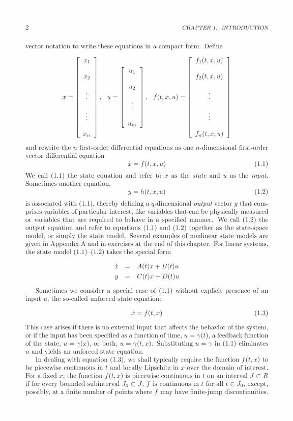
vector notation to write these equations in a compact form. Define
x =
⎡⎢⎢⎢⎢⎢⎢⎢⎢⎢⎢⎢⎢⎢⎢⎣
x1
x2
...
...
xn
⎤⎥⎥⎥⎥⎥⎥⎥⎥⎥⎥⎥⎥⎥⎥⎦
, u =
⎡⎢⎢⎢⎢⎢⎢⎢⎢⎢⎣
u1
u2
...
um
⎤⎥⎥⎥⎥⎥⎥⎥⎥⎥⎦
, f(t, x, u) =
⎡⎢⎢⎢⎢⎢⎢⎢⎢⎢⎢⎢⎢⎢⎢⎣
f1(t, x, u)
f2(t, x, u)
...
...
fn(t, x, u)
⎤⎥⎥⎥⎥⎥⎥⎥⎥⎥⎥⎥⎥⎥⎥⎦
and rewrite the n first-order differential equations as one n-dimensional first-ordervector differential equation
x = f(t, x, u) (1.1)
We call (1.1) the state equation and refer to x as the state and u as the input.Sometimes another equation,
y = h(t, x, u) (1.2)
is associated with (1.1), thereby defining a q-dimensional output vector y that com-prises variables of particular interest, like variables that can be physically measuredor variables that are required to behave in a specified manner. We call (1.2) theoutput equation and refer to equations (1.1) and (1.2) together as the state-spacemodel, or simply the state model. Several examples of nonlinear state models aregiven in Appendix A and in exercises at the end of this chapter. For linear systems,the state model (1.1)–(1.2) takes the special form
x = A(t)x + B(t)uy = C(t)x + D(t)u
Sometimes we consider a special case of (1.1) without explicit presence of aninput u, the so-called unforced state equation:
x = f(t, x) (1.3)
This case arises if there is no external input that affects the behavior of the system,or if the input has been specified as a function of time, u = γ(t), a feedback functionof the state, u = γ(x), or both, u = γ(t, x). Substituting u = γ in (1.1) eliminatesu and yields an unforced state equation.
In dealing with equation (1.3), we shall typically require the function f(t, x) tobe piecewise continuous in t and locally Lipschitz in x over the domain of interest.For a fixed x, the function f(t, x) is piecewise continuous in t on an interval J ⊂ Rif for every bounded subinterval J0 ⊂ J , f is continuous in t for all t ∈ J0, except,possibly, at a finite number of points where f may have finite-jump discontinuities.
1.1. NONLINEAR MODELS 3
This allows for cases where f(t, x) depends on an input u(t) that may experiencestep changes with time. A function f(t, x), defined for t ∈ J ⊂ R, is locallyLipschitz in x at a point x0 if there is a neighborhood N(x0, r) of x0, defined byN(x0, r) = {‖x− x0‖ < r}, and a positive constant L such that f(t, x) satisfies theLipschitz condition
‖f(t, x) − f(t, y)‖ ≤ L‖x − y‖ (1.4)
for all t ∈ J and all x, y ∈ N(x0, r), where
‖x‖ =√
xT x =√
x21 + · · · + x2
n
A function f(t, x) is locally Lipschitz in x on a domain (open and connected set)D ⊂ Rn if it is locally Lipschitz at every point x0 ∈ D. It is Lipschitz on a setW if it satisfies (1.4) for all points in W , with the same Lipschitz constant L. Alocally Lipschitz function on a domain D is not necessarily Lipschitz on D, sincethe Lipschitz condition may not hold uniformly (with the same constant L) for allpoints in D. However, a locally Lipschitz function on a domain D is Lipschitz onevery compact (closed and bounded) subset of D. A function f(t, x) is globallyLipschitz if it is Lipschitz on Rn.
When n = 1 and f depends only on x, the Lipschitz condition can be written as
|f(y) − f(x)||y − x| ≤ L
which implies that on a plot of f(x) versus x, a straight line joining any two pointsof f(x) cannot have a slope whose absolute value is greater than L. Therefore,any function f(x) that has infinite slope at some point is not locally Lipschitz atthat point. For example, any discontinuous function is not locally Lipschitz at thepoints of discontinuity. As another example, the function f(x) = x1/3 is not locallyLipschitz at x = 0 since f ′(x) = (1/3)x−2/3 → ∞ as x → 0. On the other hand, iff ′(x) is continuous at a point x0 then f(x) is locally Lipschitz at the same pointbecause continuity of f ′(x) ensures that |f ′(x)| is bounded by a constant k in aneighborhood of x0; which implies that f(x) satisfies the Lipschitz condition (1.4)over the same neighborhood with L = k.
More generally, if for t in an interval J ⊂ R and x in a domain D ⊂ Rn,the function f(t, x) and its partial derivatives ∂fi/∂xj are continuous, then f(t, x)is locally Lipschitz in x on D.1 If f(t, x) and its partial derivatives ∂fi/∂xj arecontinuous for all x ∈ Rn, then f(t, x) is globally Lipschitz in x if and only ifthe partial derivatives ∂fi/∂xj are globally bounded, uniformly in t, that is, theirabsolute values are bounded for all t ∈ J and x ∈ Rn by constants independent of(t, x).2
1See [74, Lemma 3.2] for the proof of this statement.2See [74, Lemma 3.3] for the proof of this statement.
4 CHAPTER 1. INTRODUCTION
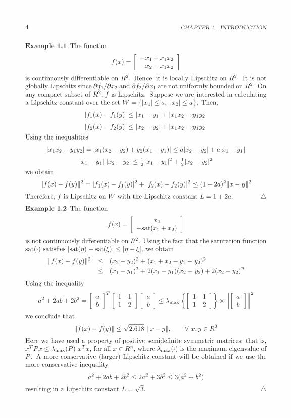
Example 1.1 The function
f(x) =[ −x1 + x1x2
x2 − x1x2
]is continuously differentiable on R2. Hence, it is locally Lipschitz on R2. It is notglobally Lipschitz since ∂f1/∂x2 and ∂f2/∂x1 are not uniformly bounded on R2. Onany compact subset of R2, f is Lipschitz. Suppose we are interested in calculatinga Lipschitz constant over the set W = {|x1| ≤ a, |x2| ≤ a}. Then,
|f1(x) − f1(y)| ≤ |x1 − y1| + |x1x2 − y1y2||f2(x) − f2(y)| ≤ |x2 − y2| + |x1x2 − y1y2|
Using the inequalities
|x1x2 − y1y2| = |x1(x2 − y2) + y2(x1 − y1)| ≤ a|x2 − y2| + a|x1 − y1||x1 − y1| |x2 − y2| ≤ 1
2 |x1 − y1|2 + 12 |x2 − y2|2
we obtain
‖f(x) − f(y)‖2 = |f1(x) − f1(y)|2 + |f2(x) − f2(y)|2 ≤ (1 + 2a)2‖x − y‖2
Therefore, f is Lipschitz on W with the Lipschitz constant L = 1 + 2a. Example 1.2 The function
f(x) =[
x2
−sat(x1 + x2)
]is not continuously differentiable on R2. Using the fact that the saturation functionsat(·) satisfies |sat(η) − sat(ξ)| ≤ |η − ξ|, we obtain
‖f(x) − f(y)‖2 ≤ (x2 − y2)2 + (x1 + x2 − y1 − y2)2
≤ (x1 − y1)2 + 2(x1 − y1)(x2 − y2) + 2(x2 − y2)2
Using the inequality
a2 + 2ab + 2b2 =[
ab
]T [ 1 11 2
] [ab
]≤ λmax
{[1 11 2
]}×∥∥∥∥[
ab
]∥∥∥∥2we conclude that
‖f(x) − f(y)‖ ≤√
2.618 ‖x − y‖, ∀ x, y ∈ R2
Here we have used a property of positive semidefinite symmetric matrices; that is,xT Px ≤ λmax(P ) xT x, for all x ∈ Rn, where λmax(·) is the maximum eigenvalue ofP . A more conservative (larger) Lipschitz constant will be obtained if we use themore conservative inequality
a2 + 2ab + 2b2 ≤ 2a2 + 3b2 ≤ 3(a2 + b2)
resulting in a Lipschitz constant L =√
3.
1.1. NONLINEAR MODELS 5
The local Lipschitz property of f(t, x) ensures local existence and uniqueness ofthe solution of the state equation (1.3), as stated in the following lemma.3
Lemma 1.1 Let f(t, x) be piecewise continuous in t and locally Lipschitz in x atx0, for all t ∈ [t0, t1]. Then, there is δ > 0 such that the state equation x = f(t, x),with x(t0) = x0, has a unique solution over [t0, t0 + δ]. �
Without the local Lipschitz condition, we cannot ensure uniqueness of the solu-tion. For example, the state equation x = x1/3, whose right-hand side function iscontinuous but not locally Lipschitz at x = 0, has x(t) = (2t/3)3/2 and x(t) ≡ 0 astwo different solutions when the initial state is x(0) = 0.
Lemma 1.1 is a local result because it guarantees existence and uniqueness ofthe solution over an interval [t0, t0 + δ], but this interval might not include a giveninterval [t0, t1]. Indeed the solution may cease to exist after some time.
Example 1.3 In the one-dimensional system x = −x2, the function f(x) = −x2
is locally Lipschitz for all x. Yet, when we solve the equation with x(0) = −1, thesolution x(t) = 1/(t − 1) tends to −∞ as t → 1. The phrase “finite escape time” is used to describe the phenomenon that a solutionescapes to infinity at finite time. In Example 1.3, we say that the solution has afinite escape time at t = 1.
In the forthcoming Lemmas 1.2 and 1.3,4 we shall give conditions for globalexistence and uniqueness of solutions. Lemma 1.2 requires the function f to beglobally Lipschitz, while Lemma 1.3 requires f to be only locally Lipschitz, butwith an additional requirement that the solution remains bounded. Note that thefunction f(x) = −x2 of Example 1.3 is locally Lipschitz for all x but not globallyLipschitz because f ′(x) = −2x is not globally bounded.
Lemma 1.2 Let f(t, x) be piecewise continuous in t and globally Lipschitz in x forall t ∈ [t0, t1]. Then, the state equation x = f(t, x), with x(t0) = x0, has a uniquesolution over [t0, t1]. �
The global Lipschitz condition is satisfied for linear systems of the form
x = A(t)x + g(t)
when ‖A(t)‖ ≤ L for all t ≥ t0, but it is a restrictive condition for general nonlinearsystems. The following lemma avoids this condition.
Lemma 1.3 Let f(t, x) be piecewise continuous in t and locally Lipschitz in x forall t ≥ t0 and all x in a domain D ⊂ Rn. Let W be a compact (closed and bounded)subset of D, x0 ∈ W , and suppose it is known that every solution of
x = f(t, x), x(t0) = x0
lies entirely in W . Then, there is a unique solution that is defined for all t ≥ t0. �
3See [74, Theorem 3.1] for the proof of Lemma 1.1. See [56, 62, 95] for a deeper look into exis-tence and uniqueness of solutions, and the qualitative behavior of nonlinear differential equations.
4See [74, Theorem 3.2] and [74, Theorem 3.3] for the proofs of Lemmas 1.2 and 1.3, respectively.
6 CHAPTER 1. INTRODUCTION
The trick in applying Lemma 1.3 is in checking the assumption that every so-lution lies in a compact set without solving the state equation. We will see inChapter 3 that Lyapunov’s method for stability analysis provides a tool to ensurethis property. For now, let us illustrate the application of the lemma by an example.
Example 1.4 Consider the one-dimensional system
x = −x3 = f(x)
The function f(x) is locally Lipschitz on R, but not globally Lipschitz becausef ′(x) = −3x2 is not globally bounded. If, at any instant of time, x(t) is positive,the derivative x(t) will be negative and x(t) will be decreasing. Similarly, if x(t) isnegative, the derivative x(t) will be positive and x(t) will be increasing. Therefore,starting from any initial condition x(0) = a, the solution cannot leave the compactset {|x| ≤ |a|}. Thus, we conclude by Lemma 1.3 that the equation has a uniquesolution for all t ≥ 0.
A special case of (1.3) arises when the function f does not depend explicitly ont; that is,
x = f(x)
in which case the state equation is said to be autonomous or time invariant. Thebehavior of an autonomous system is invariant to shifts in the time origin, sincechanging the time variable from t to τ = t−a does not change the right-hand side ofthe state equation. If the system is not autonomous, then it is called nonautonomousor time varying.
More generally, the state model (1.1)–(1.2) is said to be time invariant if thefunctions f and h do not depend explicitly on t; that is,
x = f(x, u), y = h(x, u)
If either f or h depends on t, the state model is said to be time varying. A time-invariant state model has a time-invariance property with respect to shifting theinitial time from t0 to t0 + a, provided the input waveform is applied from t0 + ainstead of t0. In particular, let (x(t), y(t)) be the response for t ≥ t0 to initial statex(t0) = x0 and input u(t) applied for t ≥ t0, and let (x(t), y(t)) be the response fort ≥ t0 + a to initial state x(t0 + a) = x0 and input u(t) applied for t ≥ t0 + a. Now,take x0 = x0 and u(t) = u(t− a) for t ≥ t0 + a. By changing the time variable fromt to t − a it can be seen that x(t) = x(t − a) and y(t) = y(t − a) for t ≥ t0 + a.Therefore, for time-invariant systems, we can, without loss of generality, take theinitial time to be t0 = 0.
A useful analysis tool is to transform the state equation from the x-coordinatesto the z-coordinates by the change of variables z = T (x). For linear systems, thechange of variables is a similarity transformation z = Px, where P is a nonsingularmatrix. For a nonlinear change of variables, z = T (x), the map T must be invertible;that is, it must have an inverse map T−1(·) such that x = T−1(z) for all z ∈ T (D),

1.1. NONLINEAR MODELS 7
where D is the domain of T . Moreover, because the derivatives of z and x shouldbe continuous, we require both T (·) and T−1(·) to be continuously differentiable. Acontinuously differentiable map with a continuously differentiable inverse is knownas a diffeomorphism. A map T (x) is a local diffeomorphism at a point x0 if thereis a neighborhood N of x0 such that T restricted to N is a diffeomorphism on N .It is a global diffeomorphism if it is a diffeomorphism on Rn and T (Rn) = Rn.The following lemma gives conditions on a map z = T (x) to be a local or globaldiffeomorphism using the Jacobian matrix [∂T/∂x], which is a square matrix whose(i, j) element is the partial derivative ∂Ti/∂xj .5
Lemma 1.4 The continuously differentiable map z = T (x) is a local diffeomor-phism at x0 if the Jacobian matrix [∂T/∂x] is nonsingular at x0. It is a globaldiffeomorphism if and only if [∂T/∂x] is nonsingular for all x ∈ Rn and T isproper; that is, lim‖x‖→∞ ‖T (x)‖ = ∞. �
Example 1.5 In Section A.4 two different models of the negative resistance oscil-lator are given, which are related by the change of variables
z = T (x) =[−h(x1) − x2/ε
x1
]
Assuming that h(x1) is continuously differentiable, the Jacobian matrix is
∂T
∂x=
⎡⎣∂T1
∂x1
∂T1∂x2
∂T2∂x1
∂T2∂x2
⎤⎦ =
[−h′(x1) −1/ε1 0
]
Its determinant, 1/ε, is positive for all x. Moreover, T (x) is proper because
‖T (x)‖2 = [h(x1) + x2/ε]2 + x21
which shows that lim‖x‖→∞ ‖T (x)‖ = ∞. In particular, if |x1| → ∞, so is ‖T (x)‖.If |x1| is finite while |x2| → ∞, so is [h(x1) + x2/ε]2 and consequently ‖T (x)‖.
Equilibrium points are important features of the state equation. A point x∗ isan equilibrium point of x = f(t, x) if the equation has a constant solution x(t) ≡ x∗.For the time-invariant system x = f(x), equilibrium points are the real solutions of
f(x) = 0
An equilibrium point could be isolated; that is, there are no other equilibrium pointsin its vicinity, or there could be a continuum of equilibrium points. The linearsystem x = Ax has an isolated equilibrium point at x = 0 when A is nonsingularor a continuum of equilibrium points in the null space of A when A is singular. It
5The proof of the local result follows from the inverse function theorem [3, Theorem 7-5]. Theproof of the global results can be found in [117] or [150].

8 CHAPTER 1. INTRODUCTION
cannot have multiple isolated equilibrium points, for if xa and xb are two equilibriumpoints, then by linearity any point on the line αxa +(1−α)xb connecting xa and xb
will be an equilibrium point. A nonlinear state equation can have multiple isolatedequilibrium points. For example, the pendulum equation
x1 = x2, x2 = − sin x1 − bx2
has equilibrium points at (x1 = nπ, x2 = 0) for n = 0,±1,±2, · · · .
1.2 Nonlinear Phenomena
The powerful analysis tools for linear systems are founded on the basis of the su-perposition principle. As we move from linear to nonlinear systems, we are facedwith a more difficult situation. The superposition principle no longer holds, andanalysis involves more advanced mathematics. Because of the powerful tools weknow for linear systems, the first step in analyzing a nonlinear system is usually tolinearize it, if possible, about some nominal operating point and analyze the result-ing linear model. This is a common practice in engineering, and it is a useful one.However, there are two basic limitations of linearization. First, since linearizationis an approximation in the neighborhood of an operating point, it can only pre-dict the “local” behavior of the nonlinear system in the vicinity of that point. Itcannot predict the “nonlocal” behavior far from the operating point and certainlynot the “global” behavior throughout the state space. Second, the dynamics ofa nonlinear system are much richer than the dynamics of a linear system. Thereare “essentially nonlinear phenomena” that can take place only in the presence ofnonlinearity; hence, they cannot be described or predicted by linear models. Thefollowing are examples of essentially nonlinear phenomena:
• Finite escape time. The state of an unstable linear system goes to infinityas time approaches infinity; a nonlinear system’s state, however, can go toinfinity in finite time.
• Multiple isolated equilibria. A linear system can have only one isolated equi-librium point; thus, it can have only one steady-state operating point thatattracts the state of the system irrespective of the initial state. A nonlinearsystem can have more than one isolated equilibrium point. The state mayconverge to one of several steady-state operating points, depending on theinitial state of the system.
• Limit cycles. For a linear time-invariant system to oscillate, it must have apair of eigenvalues on the imaginary axis, which is a nonrobust condition thatis almost impossible to maintain in the presence of perturbations. Even if wedo so, the amplitude of oscillation will be dependent on the initial state. Inreal life, stable oscillation must be produced by nonlinear systems. There are
1.3. OVERVIEW OF THE BOOK 9
nonlinear systems that can go into oscillation of fixed amplitude and frequency,irrespective of the initial state. This type of oscillation is known as limit cycles.
• Subharmonic, harmonic, or almost-periodic oscillations. A stable linear sys-tem under a periodic input produces a periodic output of the same frequency.A nonlinear system under periodic excitation can oscillate with frequenciesthat are submultiples or multiples of the input frequency. It may even gener-ate an almost-periodic oscillation, an example of which is the sum of periodicoscillations with frequencies that are not multiples of each other.
• Chaos. A nonlinear system can have a more complicated steady-state behaviorthat is not equilibrium, periodic oscillation, or almost-periodic oscillation.Such behavior is usually referred to as chaos. Some of these chaotic motionsexhibit randomness, despite the deterministic nature of the system.
• Multiple modes of behavior. It is not unusual for two or more modes of be-havior to be exhibited by the same nonlinear system. An unforced systemmay have more than one limit cycle. A forced system with periodic excita-tion may exhibit harmonic, subharmonic, or more complicated steady-statebehavior, depending upon the amplitude and frequency of the input. It mayeven exhibit a discontinuous jump in the mode of behavior as the amplitudeor frequency of the excitation is smoothly changed.
In this book, we encounter only the first three of these phenomena.6 The phe-nomenon of finite escape time has been already demonstrated in Example 1.3, whilemultiple equilibria and limit cycles will be introduced in the next chapter.
1.3 Overview of the Book
Our study of nonlinear control starts with nonlinear analysis tools that will beused in the analysis and design of nonlinear control systems. Chapter 2 introducesphase portraits for the analysis of two-dimensional systems and illustrates someessentially nonlinear phenomena. The next five chapters deal with stability analy-sis of nonlinear systems. Stability of equilibrium points is defined and studied inChapter 3 for time-invariant systems. After presenting some preliminary results forlinear systems, linearization, and one-dimensional systems, the technique of Lya-punov stability is introduced. It is the main tool for stability analysis of nonlinearsystems. It requires the search for a scalar function of the state, called Lyapunovfunction, such that the function and its time derivative satisfy certain conditions.The challenge in Lyapunov stability is the search for a Lyapunov function. How-ever, by the time we reach the end of Chapter 7, the reader would have seen manyideas and examples of how to find Lyapunov functions. Additional ideas are given
6To read about forced oscillation, chaos, bifurcation, and other important topics, consult [52,55, 136, 146].
10 CHAPTER 1. INTRODUCTION
in Appendix C. Chapter 4 extends Lyapunov stability to time-varying systems andshows how it can be useful in the analysis of perturbed system. This leads into thenotion of input-to-state stability. Chapter 5 deals with a special class of systemsthat dissipates energy. One point we emphasize is the connection between passivityand Lyapunov stability. Chapter 6 looks at input-output stability and shows thatit can be established using Lyapunov functions. The tools of Chapters 5 and 6 areused in Chapter 7 to derive stability criteria for the feedback connection of twostable systems.
The next six chapters deal with nonlinear control. Chapter 8 presents somespecial nonlinear forms that play significant roles in the design of nonlinear con-trollers. Chapters 9 to 13 deal with nonlinear control problems, including nonlinearobservers. The nonlinear control techniques we are going to study can be catego-rized into five different approaches to deal with nonlinearity. These are:
• Approximate nonlinearity• Compensate for nonlinearity• Dominate nonlinearity• Use intrinsic properties• Divide and conquer
Linearization is the prime example of approximating nonlinearities. Feedback lin-earization that cancels nonlinearity is an example of nonlinearity compensation.Robust control techniques, which are built around the classical tool of high-gainfeedback, dominate nonlinearities. Passivity-based control is an example of a tech-nique that takes advantage of an intrinsic property of the system. Because thecomplexity of a nonlinear system grows rapidly with dimension, one of the effectiveideas is to decompose the system into lower-order components, which might be eas-ier to analyze and design, then build up back to the original system. Backsteppingis an example of this divide and conquer approach.
Four appendices at the end of the book give examples of nonlinear state models,mathematical background, procedures for constructing composite Lyapunov func-tions, and proofs of some results. The topics in this book overlap with topics insome excellent textbooks, which can be consulted for further reading. The list in-cludes [10, 53, 63, 66, 92, 118, 129, 132, 144]. The main source for the material inthis book is [74], which was prepared using many references. The reader is advisedto check the Notes and References section of [74] for a detailed account of thesereferences.
1.4 Exercises
1.1 A mathematical model that describes a wide variety of single-input–single-ouput nonlinear systems is the nth-order differential equation
y(n) = g(t, y, y, . . . , y(n−1), u
)where u is the input and y the output. Find a state model.

1.4. EXERCISES 11
1.2 The nonlinear dynamic equations for a single-link manipulator with flexiblejoints [135], damping ignored, is given by
Iq1 + MgL sin q1 + k(q1 − q2) = 0, Jq2 − k(q1 − q2) = u
where q1 and q2 are angular positions, I and J are moments of inertia, k is a springconstant, M is the total mass, L is a distance, and u is a torque input.
(a) Using q1, q1, q2, and q2 as state variables, find the state equation.
(b) Show that the right-hand side function is globally Lipschitz when u is constant.
(c) Find the equilibrium points when u = 0.
1.3 A synchronous generator connected to an infinite bus is represented by [103]
Mδ = P − Dδ − η1Eq sin δ, τEq = −η2Eq + η3 cos δ + EF
where δ is an angle in radians, Eq is voltage, P is mechanical input power, EF isfield voltage (input), D is damping coefficient, M is inertial coefficient, τ is timeconstant, and η1, η2, and η3 are positive parameters.
(a) Using δ, δ, and Eq as state variables, find the state equation.
(b) Show that the right-hand side function is locally Lipschitz when P and EF areconstant. Is it globally Lipschitz?
(c) Show that when P and EF are constant and 0 < P < η1EF /η2, there is aunique equilibrium point in the region 0 ≤ δ ≤ π/2.
1.4 The circuit shown in Figure 1.1 contains a nonlinear inductor and is drivenby a time-dependent current source. Suppose the nonlinear inductor is a Josephsonjunction [25] described by iL = I0 sin kφL, where φL is the magnetic flux of theinductor and I0 and k are constants.
(a) Using φL and vC as state variables, find the state equation.
(b) Show that the right-hand side function is locally Lipschitz when is is constant.Is it globally Lipschitz?
(c) Find the equilibrium points when is = Is (constant) with 0 < Is < I0.
1.5 Repeat the previous exercise when the nonlinear inductor is described by iL =k1φL + k2φ
3L, where k1 and k2 are positive constants. In Part (b), Is > 0.
1.6 Figure 1.2 shows a vehicle moving on a road with grade angle θ, where v thevehicle’s velocity, M is its mass, and F is the tractive force generated by the engine.Assume that the friction is due to Coulomb friction, linear viscous friction, and adrag force proportional to v2. Viewing F as the control input and θ as a disturbanceinput, find a state model of the system.
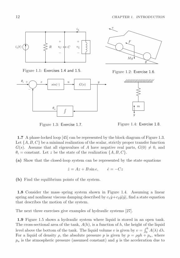
12 CHAPTER 1. INTRODUCTION
vC
iL
vLis(t) R C
+ +
−−
Figure 1.1: Exercises 1.4 and 1.5.
F
Mgθ
v
Figure 1.2: Exercise 1.6.
θo
θi e u y+
−s in (.) G (s)
Figure 1.3: Exercise 1.7.
m
y
Figure 1.4: Exercise 1.8.
1.7 A phase-locked loop [45] can be represented by the block diagram of Figure 1.3.Let {A,B,C} be a minimal realization of the scalar, strictly proper transfer functionG(s). Assume that all eigenvalues of A have negative real parts, G(0) �= 0, andθi = constant. Let z be the state of the realization {A,B,C}.(a) Show that the closed-loop system can be represented by the state equations
z = Az + B sin e, e = −Cz
(b) Find the equilibrium points of the system.
1.8 Consider the mass–spring system shown in Figure 1.4. Assuming a linearspring and nonlinear viscous damping described by c1y+c2y|y|, find a state equationthat describes the motion of the system.
The next three exercises give examples of hydraulic systems [27].
1.9 Figure 1.5 shows a hydraulic system where liquid is stored in an open tank.The cross-sectional area of the tank, A(h), is a function of h, the height of the liquidlevel above the bottom of the tank. The liquid volume v is given by v =
∫ h
0A(λ) dλ.
For a liquid of density ρ, the absolute pressure p is given by p = ρgh + pa, wherepa is the atmospheric pressure (assumed constant) and g is the acceleration due to

1.4. EXERCISES 13
wi
pa
wo
pa
h
p k
+Δp−
Figure 1.5: Exercise 1.9.
wowi
pa
pa
p
pa
k
+Δp−−Δp+
Figure 1.6: Exercise 1.10.
gravity. The tank receives liquid at a flow rate wi and loses liquid through a valvethat obeys the flow-pressure relationship wo = k
√p − pa. The rate of change of v
satisfies v = wi − wo. Take wi to be the control input and h to be the output.
(a) Using h as the state variable, determine the state model.
(b) Using p − pa as the state variable, determine the state model.
(c) Find a constant input that maintains a constant output at h = r.
1.10 The hydraulic system shown in Figure 1.6 consists of a constant speed cen-trifugal pump feeding a tank from which liquid flows through a pipe and a valvethat obeys the relationship wo = k
√p − pa. The pressure-flow characteristic of the
pump is given by p − pa = β√
1 − wi/α for some positive constants α and β. Thecross-sectional area of the tank is uniform; therefore, v = Ah and p = pa + ρgv/A,where the variables are defined in the previous exercise.
(a) Using (p − pa) as the state variable, find the state model.
(b) Find the equilibrium points of the system.
1.11 The valves in the hydraulic system of Figure 1.7 obey the flow relationshipsw1 = k1
√p1 − p2 and w2 = k2
√p2 − pa. The pump characteristic is p1 − pa =
β√
1 − wp/α. All variables are defined in the previous two exercises.
(a) Using (p1 − pa) and (p2 − pa) as the state variables, find the state equation.
(b) Find the equilibrium points of the system.
1.12 For each of the following systems, investigate local and global Lipschitz prop-erties. Assume that input variables are continuous functions of time.
(a) The pendulum equation (A.2).
(b) The mass-spring system (A.6).

14 CHAPTER 1. INTRODUCTION
pa
p1w1k1 w2k2
wp
pa
pa
pa
p2
Figure 1.7: The hydraulic system of Exercise 1.11.
(c) The tunnel diode circuit (A.7).
(d) The van der Pol oscillator (A.13).
(e) The boost converter (A.16).
(f) The biochemical reactor (A.19) with ν defined by (A.20).
(g) The DC motor (A.25) when fe and f� are linear functions.
(h) The magnetic levitation system (A.30)–(A.32).
(i) The electrostatic actuator (A.33).
(j) The two-link robot manipulator (A.35)–(A.37).
(k) The inverted pendulum on a cart (A.41)–(A.44).
(l) The TORA system (A.49)–(A.52).
1.13 Find a global diffeomorphism z = T (x) that transforms the system
x1 = x2 + g1(x1), x2 = x3 + g2(x1, x2), x3 = g3(x) + g4(x)u, y = x1
intoz1 = z2, z2 = z3, z3 = a(z) + b(z)u, y = z1
Assume g1 to g4 are smooth.
1.14 Find a diffeomorphism z = T (x) that transforms the system
x1 = sin x2, x2 = −x21 + u, y = x1
intoz1 = z2, z2 = a(z) + b(z)u, y = z1
and give the definitions of a and b.
Chapter 2
Two-Dimensional Systems
Two-dimensional time-invariant systems occupy an important place in the study ofnonlinear systems because solutions can be represented by curves in the plane. Thisallows for easy visualization of the qualitative behavior of the system. The purposeof this chapter is to use two-dimensional systems to introduce, in an elementarycontext, some of the basic ideas of nonlinear systems. In particular, we will look atthe behavior of a nonlinear system near equilibrium points and the phenomenon ofnonlinear oscillation.1
A two-dimensional time-invariant system is represented by two simultaneousdifferential equations
x1 = f1(x1, x2), x2 = f2(x1, x2) (2.1)
Assume that f1 and f2 are locally Lipschitz over the domain of interest and letx(t) = (x1(t), x2(t)) be the solution of (2.1) that starts at x(0) = (x10, x20)
def= x0.The locus in the x1–x2 plane of the solution x(t) for all t ≥ 0 is a curve that passesthrough the point x0. This curve is called a trajectory or orbit of (2.1) from x0.The x1–x2 plane is called the state plane or phase plane. Using vector notation werewrite (2.1) as
x = f(x)
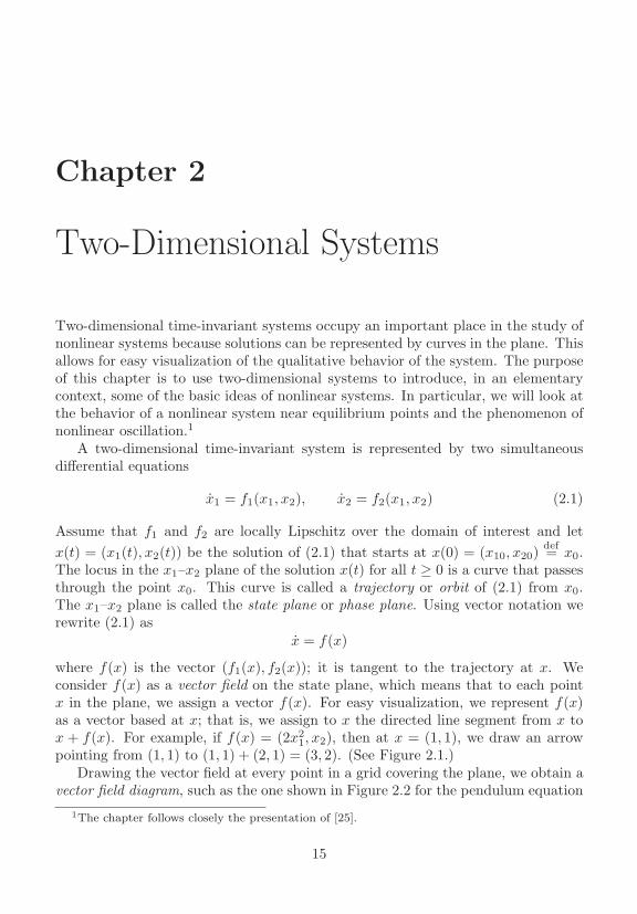
where f(x) is the vector (f1(x), f2(x)); it is tangent to the trajectory at x. Weconsider f(x) as a vector field on the state plane, which means that to each pointx in the plane, we assign a vector f(x). For easy visualization, we represent f(x)as a vector based at x; that is, we assign to x the directed line segment from x tox + f(x). For example, if f(x) = (2x2
1, x2), then at x = (1, 1), we draw an arrowpointing from (1, 1) to (1, 1) + (2, 1) = (3, 2). (See Figure 2.1.)
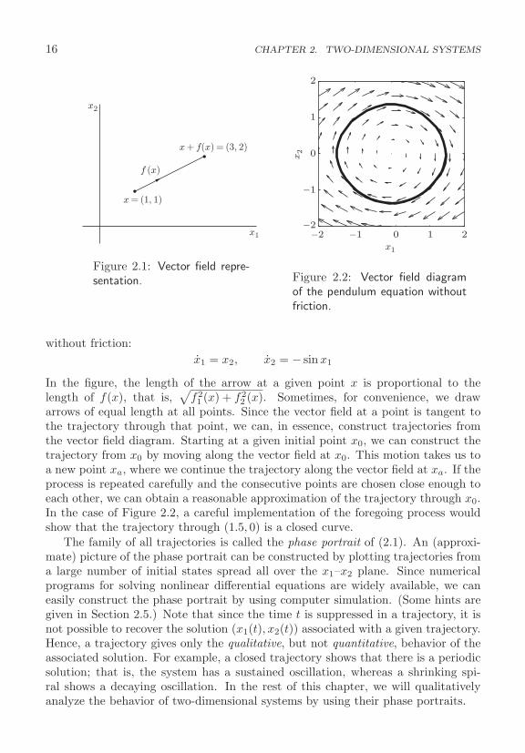
Drawing the vector field at every point in a grid covering the plane, we obtain avector field diagram, such as the one shown in Figure 2.2 for the pendulum equation
1The chapter follows closely the presentation of [25].
15
16 CHAPTER 2. TWO-DIMENSIONAL SYSTEMS
x2
x1
f (x)
x = (1, 1)
x + f(x) = (3, 2)
Figure 2.1: Vector field repre-sentation.
−2 −1 0 1 2−2
−1
0
1
2
x1
x2
Figure 2.2: Vector field diagramof the pendulum equation withoutfriction.
without friction:x1 = x2, x2 = − sin x1
In the figure, the length of the arrow at a given point x is proportional to thelength of f(x), that is,
√f21 (x) + f2
2 (x). Sometimes, for convenience, we drawarrows of equal length at all points. Since the vector field at a point is tangent tothe trajectory through that point, we can, in essence, construct trajectories fromthe vector field diagram. Starting at a given initial point x0, we can construct thetrajectory from x0 by moving along the vector field at x0. This motion takes us toa new point xa, where we continue the trajectory along the vector field at xa. If theprocess is repeated carefully and the consecutive points are chosen close enough toeach other, we can obtain a reasonable approximation of the trajectory through x0.In the case of Figure 2.2, a careful implementation of the foregoing process wouldshow that the trajectory through (1.5, 0) is a closed curve.
The family of all trajectories is called the phase portrait of (2.1). An (approxi-mate) picture of the phase portrait can be constructed by plotting trajectories froma large number of initial states spread all over the x1–x2 plane. Since numericalprograms for solving nonlinear differential equations are widely available, we caneasily construct the phase portrait by using computer simulation. (Some hints aregiven in Section 2.5.) Note that since the time t is suppressed in a trajectory, it isnot possible to recover the solution (x1(t), x2(t)) associated with a given trajectory.Hence, a trajectory gives only the qualitative, but not quantitative, behavior of theassociated solution. For example, a closed trajectory shows that there is a periodicsolution; that is, the system has a sustained oscillation, whereas a shrinking spi-ral shows a decaying oscillation. In the rest of this chapter, we will qualitativelyanalyze the behavior of two-dimensional systems by using their phase portraits.
2.1. QUALITATIVE BEHAVIOR OF LINEAR SYSTEMS 17
2.1 Qualitative Behavior of Linear Systems
Consider the linear time-invariant system
x = Ax (2.2)
where A is a 2 × 2 real matrix. The solution of (2.2) for a given initial state x0 isgiven by
x(t) = M exp(Jrt)M−1x0
where Jr is the real Jordan form of A and M is a real nonsingular matrix suchthat M−1AM = Jr. We restrict our attention to the case when A has distincteigenvalues, different from zero.2 The real Jordan form takes one of two forms[
λ1 00 λ2
]or
[α −ββ α
]
The first form occurs when the eigenvalues are real and the second when they arecomplex.
Case 1. Both eigenvalues are real
In this case, M = [v1, v2], where v1 and v2 are the real eigenvectors associatedwith λ1 and λ2. The change of coordinates z = M−1x transforms the system intotwo decoupled scalar (one-dimensional) differential equations,
z1 = λ1z1, z2 = λ2z2
whose solutions, for a given initial state (z10, z20), are given by
z1(t) = z10eλ1t, z2(t) = z20e
λ2t
Eliminating t between the two equations, we obtain
z2 = czλ2/λ11 (2.3)
where c = z20/(z10)(λ2/λ1). The phase portrait of the system is given by the familyof curves generated from (2.3) by allowing the real number c to take arbitrary values.The shape of the phase portrait depends on the signs of λ1 and λ2.
Consider first the case when both eigenvalues are negative. Without loss ofgenerality, let λ2 < λ1 < 0. Here, both exponential terms eλ1t and eλ2t tend tozero as t → ∞. Moreover, since λ2 < λ1 < 0, the term eλ2t tends to zero fasterthan eλ1t. Hence, we call λ2 the fast eigenvalue and λ1 the slow eigenvalue. Forlater reference, we call v2 the fast eigenvector and v1 the slow eigenvector. The
2See [74, Section 2.1] for the case when A has zero or multiple eigenvalues.
18 CHAPTER 2. TWO-DIMENSIONAL SYSTEMS
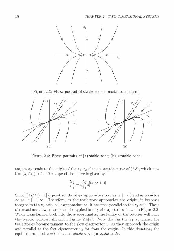
z2
z1
Figure 2.3: Phase portrait of stable node in modal coordinates.
x2 x2v2 v2
v1 v1
x1 x1
(a) (b)
Figure 2.4: Phase portraits of (a) stable node; (b) unstable node.
trajectory tends to the origin of the z1–z2 plane along the curve of (2.3), which nowhas (λ2/λ1) > 1. The slope of the curve is given by
dz2
dz1= c
λ2
λ1z[(λ2/λ1)−1]1
Since [(λ2/λ1)−1] is positive, the slope approaches zero as |z1| → 0 and approaches∞ as |z1| → ∞. Therefore, as the trajectory approaches the origin, it becomestangent to the z1-axis; as it approaches ∞, it becomes parallel to the z2-axis. Theseobservations allow us to sketch the typical family of trajectories shown in Figure 2.3.When transformed back into the x-coordinates, the family of trajectories will havethe typical portrait shown in Figure 2.4(a). Note that in the x1–x2 plane, thetrajectories become tangent to the slow eigenvector v1 as they approach the originand parallel to the fast eigenvector v2 far from the origin. In this situation, theequilibrium point x = 0 is called stable node (or nodal sink).
2.1. QUALITATIVE BEHAVIOR OF LINEAR SYSTEMS 19
x2z2
z1
v2 v1
x1
(a) (b)
Figure 2.5: Phase portrait of a saddle point (a) in modal coordinates; (b) in originalcoordinates.
When λ1 and λ2 are positive, the phase portrait will retain the character of Fig-ure 2.4(a), but with the trajectory directions reversed, since the exponential termseλ1t and eλ2t grow exponentially as t increases. Figure 2.4(b) shows the phase por-trait for the case λ2 > λ1 > 0. The equilibrium point x = 0 is referred to in thisinstance as unstable node (or nodal source).
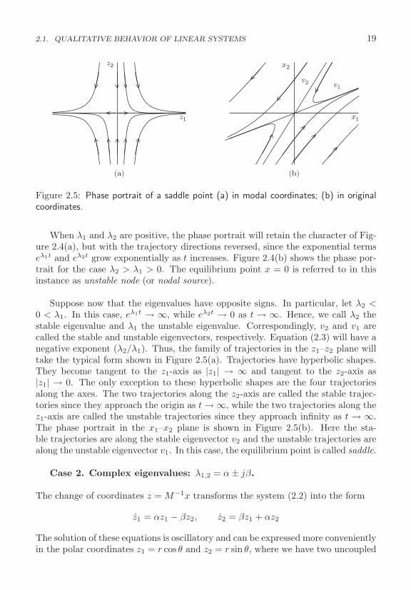
Suppose now that the eigenvalues have opposite signs. In particular, let λ2 <0 < λ1. In this case, eλ1t → ∞, while eλ2t → 0 as t → ∞. Hence, we call λ2 thestable eigenvalue and λ1 the unstable eigenvalue. Correspondingly, v2 and v1 arecalled the stable and unstable eigenvectors, respectively. Equation (2.3) will have anegative exponent (λ2/λ1). Thus, the family of trajectories in the z1–z2 plane willtake the typical form shown in Figure 2.5(a). Trajectories have hyperbolic shapes.They become tangent to the z1-axis as |z1| → ∞ and tangent to the z2-axis as|z1| → 0. The only exception to these hyperbolic shapes are the four trajectoriesalong the axes. The two trajectories along the z2-axis are called the stable trajec-tories since they approach the origin as t → ∞, while the two trajectories along thez1-axis are called the unstable trajectories since they approach infinity as t → ∞.The phase portrait in the x1–x2 plane is shown in Figure 2.5(b). Here the sta-ble trajectories are along the stable eigenvector v2 and the unstable trajectories arealong the unstable eigenvector v1. In this case, the equilibrium point is called saddle.
Case 2. Complex eigenvalues: λ1,2 = α ± jβ.
The change of coordinates z = M−1x transforms the system (2.2) into the form
z1 = αz1 − βz2, z2 = βz1 + αz2
The solution of these equations is oscillatory and can be expressed more convenientlyin the polar coordinates z1 = r cos θ and z2 = r sin θ, where we have two uncoupled

20 CHAPTER 2. TWO-DIMENSIONAL SYSTEMS
z1 z1 z1
z2 z2 z2
(a) (b) (c)
Figure 2.6: Typical trajectories in the case of complex eigenvalues.(a) α < 0; (b) α > 0; (c) α = 0.
x2 x2 x2
x1 x1 x1
(a) (b) (c)
Figure 2.7: Phase portraits of (a) stable focus; (b) unstable focus; (c) center.
scalar differential equations:
r = αr and θ = β
The solution for a given initial state (r0, θ0) is given by
r(t) = r0eαt and θ(t) = θ0 + βt
which define a logarithmic spiral in the z1–z2 plane. Depending on the value of α,the trajectory will take one of the three forms shown in Figure 2.6. When α < 0,the spiral converges to the origin; when α > 0, it diverges away from the origin.When α = 0, the trajectory is a circle of radius r0. Figure 2.7 shows the trajectoriesin the x1–x2 plane. The equilibrium point x = 0 is referred to as stable focus (orspiral sink) if α < 0, unstable focus (or spiral source) if α > 0, and center if α = 0.
The local behavior of a nonlinear system near an equilibrium point may bededuced by linearizing the system about that point and studying the behavior ofthe resultant linear system. How conclusive this linearization is, depends to a greatextent on how the various qualitative phase portraits of a linear system persistunder perturbations. We can gain insight into the behavior of a linear systemunder perturbations by examining the special case of linear perturbations. SupposeA is perturbed to A + ΔA, where ΔA is a 2 × 2 real matrix whose elements havearbitrarily small magnitudes. From the perturbation theory of matrices,3 we know
3See [51, Chapter 7].
2.2. QUALITATIVE BEHAVIOR NEAR EQUILIBRIUM POINTS 21
that the eigenvalues of a matrix depend continuously on its parameters. This meansthat, given any positive number ε, there is a corresponding positive number δ suchthat if the magnitude of the perturbation in each element of A is less than δ, theeigenvalues of the perturbed matrix A+ΔA will lie in open discs of radius ε centeredat the eigenvalues of A. Consequently, any eigenvalue of A that lies in the openright-half plane (positive real part) or in the open left-half plane (negative real part)will remain in its respective half of the plane after arbitrarily small perturbations.On the other hand, eigenvalues on the imaginary axis, when perturbed, might gointo either the right-half or the left-half of the plane, since a disc centered on theimaginary axis will extend in both halves no matter how small ε is. Consequently,we can conclude that if the equilibrium point x = 0 of x = Ax is a node, focus,or saddle, then the equilibrium point x = 0 of x = (A + ΔA)x will be of the sametype, for sufficiently small perturbations. The situation is quite different if theequilibrium point is a center. Consider the perturbation of the real Jordan form inthe case of a center: [
μ 1−1 μ
]
where μ is a perturbation parameter. The equilibrium point of the perturbed systemis unstable focus when μ is positive, and stable focus when it is negative. This istrue no matter how small μ is, as long as it is different from zero. Because the phaseportraits of the stable and unstable foci are qualitatively different from the phaseportrait of the center, we see that a center equilibrium point may not persist underperturbations. The node, focus, and saddle equilibrium points are said to be struc-turally stable because they maintain their qualitative behavior under infinitesimallysmall perturbations,4 while the center equilibrium point is not structurally stable.The distinction between the two cases is due to the location of the eigenvalues ofA, with the eigenvalues on the imaginary axis being vulnerable to perturbations.This brings in the definition of hyperbolic equilibrium points. The equilibrium pointis hyperbolic if A has no eigenvalue with zero real part.5
2.2 Qualitative Behavior Near Equilibrium Points
In this section we will see that, except for some special cases, the qualitative behaviorof a nonlinear system near an equilibrium point can be determined via linearizationwith respect to that point.
Let p = (p1, p2) be an equilibrium point of the nonlinear system (2.1) andsuppose that the functions f1 and f2 are continuously differentiable. Expanding f1
4See [62, Chapter 16] for a rigorous and more general definition of structural stability.5This definition of hyperbolic equilibrium points extends to higher-dimensional systems. It also
carries over to equilibria of nonlinear systems by applying it to the eigenvalues of the linearizedsystem.
22 CHAPTER 2. TWO-DIMENSIONAL SYSTEMS
and f2 into their Taylor series about (p1, p2), we obtain
x1 = f1(p1, p2) + a11(x1 − p1) + a12(x2 − p2) + H.O.T.
x2 = f2(p1, p2) + a21(x1 − p1) + a22(x2 − p2) + H.O.T.
where
a11 =∂f1(x1, x2)
∂x1
∣∣∣∣x1=p1,x2=p2
, a12 =∂f1(x1, x2)
∂x2
∣∣∣∣x1=p1,x2=p2
a21 =∂f2(x1, x2)
∂x1
∣∣∣∣x1=p1,x2=p2
, a22 =∂f2(x1, x2)
∂x2
∣∣∣∣x1=p1,x2=p2
and H.O.T. denotes higher-order terms of the expansion, that is, terms of the form(x1 − p1)2, (x2 − p2)2, (x1 − p1)(x2 − p2), and so on. Since (p1, p2) is an equilibriumpoint, we have
f1(p1, p2) = f2(p1, p2) = 0
Moreover, since we are interested in the trajectories near (p1, p2), we define y1 =x1 − p1, y2 = x2 − p2, and rewrite the state equations as
y1 = x1 = a11y1 + a12y2 + H.O.T.
y2 = x2 = a21y1 + a22y2 + H.O.T.
If we restrict attention to a sufficiently small neighborhood of the equilibrium pointsuch that the higher-order terms are negligible, then we may drop these terms andapproximate the nonlinear state equations by the linear state equations
y1 = a11y1 + a12y2, y2 = a21y1 + a22y2
Rewriting the equations in a vector form, we obtain
y = Ay, where A =
⎡⎣ a11 a12
a21 a22
⎤⎦ =
⎡⎣ ∂f1
∂x1
∂f1∂x2
∂f2∂x1
∂f2∂x2
⎤⎦∣∣∣∣∣∣x=p
=∂f
∂x
∣∣∣∣x=p
The matrix [∂f/∂x] is the Jacobian of f(x), and A is its evaluation x = p.It is reasonable to expect the trajectories of the nonlinear system in a small
neighborhood of an equilibrium point to be “close” to the trajectories of its lin-earization about that point. Indeed, it is true that6 if the origin of the linearizedstate equation is a stable (respectively, unstable) node with distinct eigenvalues, astable (respectively, unstable) focus, or a saddle, then, in a small neighborhood of
6The proof of this linearization property can be found in [58]. It is valid under the assumptionthat f1(x1, x2) and f2(x1, x2) have continuous first partial derivatives in a neighborhood of theequilibrium point (p1, p2). A related, but different, linearization result will be stated in Chapter 3for higher-dimensional systems. (See Theorem 3.2.)

2.2. QUALITATIVE BEHAVIOR NEAR EQUILIBRIUM POINTS 23
the equilibrium point, the trajectories of the nonlinear state equation will behavelike a stable (respectively, unstable) node, a stable (respectively, unstable) focus, ora saddle. Consequently, we call an equilibrium point of the nonlinear state equation(2.1) stable (respectively, unstable) node, stable (respectively, unstable) focus, orsaddle if the linearized state equation about the equilibrium point has the samebehavior.
The foregoing linearization property dealt only with cases where the linearizedstate equation has no eigenvalues on the imaginary axis, that is, when the origin isa hyperbolic equilibrium point of the linear system. We extend this definition tononlinear systems and say that an equilibrium point is hyperbolic if the Jacobianmatrix, evaluated at that point, has no eigenvalues on the imaginary axis. If theJacobian matrix has eigenvalues on the imaginary axis, then the qualitative behaviorof the nonlinear state equation near the equilibrium point could be quite distinctfrom that of the linearized state equation. This should come as no surprise inview of our earlier discussion on the effect of linear perturbations on the qualitativebehavior of linear systems. The example that follows considers a case when theorigin of the linearized state equation is a center.
Example 2.1 The system
x1 = −x2 − μx1(x21 + x2
2), x2 = x1 − μx2(x21 + x2
2)
has an equilibrium point at the origin. The linearized state equation at the originhas eigenvalues ±j. Thus, the origin is a center equilibrium point for the linearizedsystem. We can determine the qualitative behavior of the nonlinear system in thepolar coordinates x1 = r cos θ, x2 = r sin θ. The equations
r = −μr3 and θ = 1
show that the trajectories of the nonlinear system will resemble a stable focus whenμ > 0 and unstable focus when μ < 0. �
The preceding example shows that the qualitative behavior describing a centerin the linearized state equation is not preserved in the nonlinear state equation. De-termining that a nonlinear system has a center must be done by nonlinear analysis.For example, by constructing the phase portrait of the pendulum equation withoutfriction, as in Figure 2.2, it can be seen that the equilibrium point at the origin(0, 0) is a center.
Determining the type of equilibrium points via linearization provides useful in-formation that should be used when we construct the phase portrait of a two-dimensional system. In fact, the first step in constructing the phase portrait shouldbe the calculation of all equilibrium points and determining the type of the isolatedones via linearization, which will give us a clear idea about the expected portrait inthe neighborhood of these equilibrium points.
24 CHAPTER 2. TWO-DIMENSIONAL SYSTEMS
2.3 Multiple Equilibria
The linear system x = Ax has an isolated equilibrium point at x = 0 if A hasno zero eigenvalues, that is, if detA �= 0. When detA = 0, the system has acontinuum of equilibrium points. These are the only possible equilibria patterns thata linear system may have. A nonlinear system can have multiple isolated equilibriumpoints. In the following two examples, we explore the qualitative behavior of thetunnel-diode circuit of Section A.3 and the pendulum equation of Section A.1. Bothsystems exhibit multiple isolated equilibria.
Example 2.2 The state model of a tunnel-diode circuit is given by
x1 =1C
[−h(x1) + x2], x2 =1L
[−x1 − Rx2 + u]
Assume that the circuit parameters are7 u = 1.2 V , R = 1.5 kΩ = 1.5 × 10³ Ω,C = 2 pF = 2 × 10⁻¹² F , and L = 5 μH = 5 × 10⁻⁶ H. Measuring time innanoseconds and the currents x2 and h(x1) in mA, the state model is given by
x1 = 0.5[−h(x1) + x2]def= f1(x)
x2 = 0.2(−x1 − 1.5x2 + 1.2) def= f2(x)
Suppose h(·) is given by
h(x1) = 17.76x1 − 103.79x21 + 229.62x3
1 − 226.31x41 + 83.72x5
1
The equilibrium points are determined by the intersection of the curve x2 = h(x1)with the load line 1.5x2 = 1.2 − x1. For the given numerical values, these twocurves intersect at three points: Q1 = (0.063, 0.758), Q2 = (0.285, 0.61), and Q3 =(0.884, 0.21), as shown by the solid curves in Figure A.5.
The Jacobian matrix of f(x) is given by
∂f
∂x=
⎡⎣ −0.5h′(x1) 0.5
−0.2 −0.3
⎤⎦
where
h′(x1) =dh
dx1= 17.76 − 207.58x1 + 688.86x2
1 − 905.24x31 + 418.6x4
1
Evaluating the Jacobian matrix at the equilibrium points Q1, Q2, and Q3, respec-
7The numerical data are taken from [25].
2.3. MULTIPLE EQUILIBRIA 25
−0.4 −0.2 0 0.2 0.4 0.6 0.8 1 1.2 1.4 1.6−0.4
−0.2
0
0.2
0.4
0.6
0.8
1
1.2
1.4
1.6
x2
Q1 Q2
Q3
x1
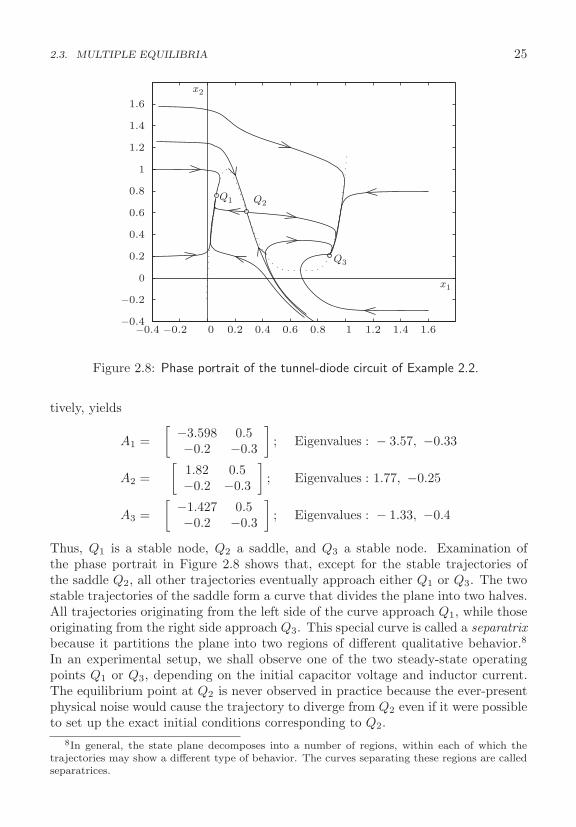
Figure 2.8: Phase portrait of the tunnel-diode circuit of Example 2.2.
tively, yields
A1 =[ −3.598 0.5
−0.2 −0.3
]; Eigenvalues : − 3.57, −0.33
A2 =[
1.82 0.5−0.2 −0.3
]; Eigenvalues : 1.77, −0.25
A3 =[ −1.427 0.5
−0.2 −0.3
]; Eigenvalues : − 1.33, −0.4
Thus, Q1 is a stable node, Q2 a saddle, and Q3 a stable node. Examination ofthe phase portrait in Figure 2.8 shows that, except for the stable trajectories ofthe saddle Q2, all other trajectories eventually approach either Q1 or Q3. The twostable trajectories of the saddle form a curve that divides the plane into two halves.All trajectories originating from the left side of the curve approach Q1, while thoseoriginating from the right side approach Q3. This special curve is called a separatrixbecause it partitions the plane into two regions of different qualitative behavior.8
In an experimental setup, we shall observe one of the two steady-state operatingpoints Q1 or Q3, depending on the initial capacitor voltage and inductor current.The equilibrium point at Q2 is never observed in practice because the ever-presentphysical noise would cause the trajectory to diverge from Q2 even if it were possibleto set up the exact initial conditions corresponding to Q2.
8In general, the state plane decomposes into a number of regions, within each of which thetrajectories may show a different type of behavior. The curves separating these regions are calledseparatrices.
26 CHAPTER 2. TWO-DIMENSIONAL SYSTEMS
The phase portrait in Figure 2.8 shows the global qualitative behavior of thetunnel-diode circuit. The bounding box is chosen so that all essential qualitativefeatures are displayed. The portrait outside the box does not contain new qualitativefeatures. �
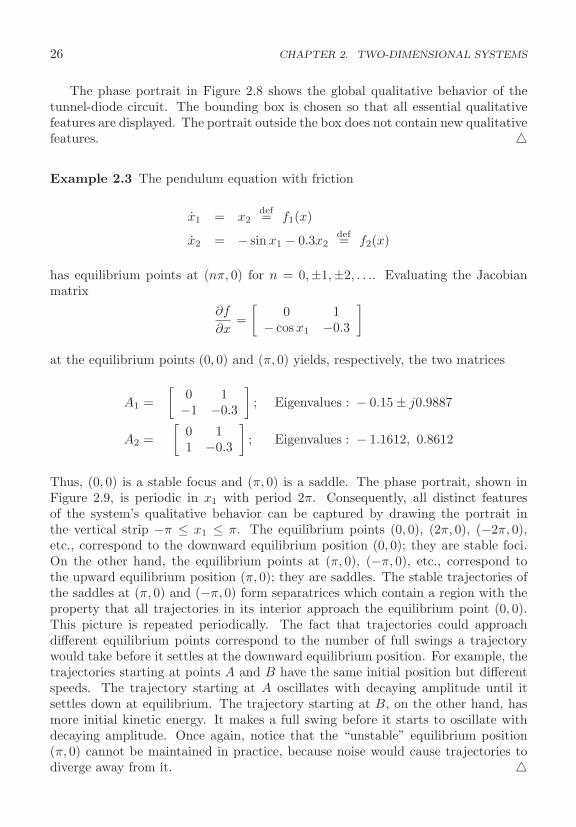
Example 2.3 The pendulum equation with friction
x1 = x2def= f1(x)
x2 = − sin x1 − 0.3x2def= f2(x)
has equilibrium points at (nπ, 0) for n = 0,±1,±2, . . .. Evaluating the Jacobianmatrix
∂f
∂x=[
0 1− cos x1 −0.3
]
at the equilibrium points (0, 0) and (π, 0) yields, respectively, the two matrices
A1 =[
0 1−1 −0.3
]; Eigenvalues : − 0.15 ± j0.9887
A2 =[
0 11 −0.3
]; Eigenvalues : − 1.1612, 0.8612
Thus, (0, 0) is a stable focus and (π, 0) is a saddle. The phase portrait, shown inFigure 2.9, is periodic in x1 with period 2π. Consequently, all distinct featuresof the system’s qualitative behavior can be captured by drawing the portrait inthe vertical strip −π ≤ x1 ≤ π. The equilibrium points (0, 0), (2π, 0), (−2π, 0),etc., correspond to the downward equilibrium position (0, 0); they are stable foci.On the other hand, the equilibrium points at (π, 0), (−π, 0), etc., correspond tothe upward equilibrium position (π, 0); they are saddles. The stable trajectories ofthe saddles at (π, 0) and (−π, 0) form separatrices which contain a region with theproperty that all trajectories in its interior approach the equilibrium point (0, 0).This picture is repeated periodically. The fact that trajectories could approachdifferent equilibrium points correspond to the number of full swings a trajectorywould take before it settles at the downward equilibrium position. For example, thetrajectories starting at points A and B have the same initial position but differentspeeds. The trajectory starting at A oscillates with decaying amplitude until itsettles down at equilibrium. The trajectory starting at B, on the other hand, hasmore initial kinetic energy. It makes a full swing before it starts to oscillate withdecaying amplitude. Once again, notice that the “unstable” equilibrium position(π, 0) cannot be maintained in practice, because noise would cause trajectories todiverge away from it. �
2.4. LIMIT CYCLES 27
−8 −6 −4 −2 0 2 4 6 8−4
−3
−2
−1
0
1
2
3
4x2
x1
B
A
Figure 2.9: Phase portrait of the pendulum equation of Example 2.3.
2.4 Limit Cycles
Oscillation is one of the most important phenomena that occur in dynamical sys-tems. A system oscillates when it has a nontrivial periodic solution
x(t + T ) = x(t), ∀ t ≥ 0
for some T > 0. The word “nontrivial” is used to exclude constant solutions corre-sponding to equilibrium points. A constant solution satisfies the preceding equation,but it is not what we have in mind when we talk of oscillation or periodic solutions.From this point on whenever we refer to a periodic solution, we will mean a nontriv-ial one. The image of a periodic solution in the phase portrait is a closed trajectory,which is usually called a periodic orbit or a closed orbit.
We have already seen an example of oscillation in Section 2.1: the two-dimensionallinear system with eigenvalues ±jβ. The origin of that system is a center and thetrajectories are closed orbits. When the system is transformed into its real Jordanform, the solution is given by
z1(t) = r0 cos(βt + θ0), z2(t) = r0 sin(βt + θ0)
where
r0 =√
z21(0) + z2
2(0), θ0 = tan−1
(z2(0)z1(0)
)Therefore, the system has a sustained oscillation of amplitude r0. It is usuallyreferred to as the harmonic oscillator. If we think of the harmonic oscillator as a
28 CHAPTER 2. TWO-DIMENSIONAL SYSTEMS
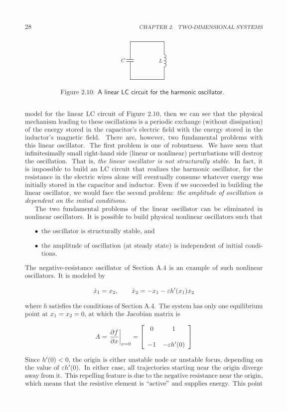
LC
Figure 2.10: A linear LC circuit for the harmonic oscillator.
model for the linear LC circuit of Figure 2.10, then we can see that the physicalmechanism leading to these oscillations is a periodic exchange (without dissipation)of the energy stored in the capacitor’s electric field with the energy stored in theinductor’s magnetic field. There are, however, two fundamental problems withthis linear oscillator. The first problem is one of robustness. We have seen thatinfinitesimally small right-hand side (linear or nonlinear) perturbations will destroythe oscillation. That is, the linear oscillator is not structurally stable. In fact, itis impossible to build an LC circuit that realizes the harmonic oscillator, for theresistance in the electric wires alone will eventually consume whatever energy wasinitially stored in the capacitor and inductor. Even if we succeeded in building thelinear oscillator, we would face the second problem: the amplitude of oscillation isdependent on the initial conditions.
The two fundamental problems of the linear oscillator can be eliminated innonlinear oscillators. It is possible to build physical nonlinear oscillators such that
• the oscillator is structurally stable, and
• the amplitude of oscillation (at steady state) is independent of initial condi-tions.
The negative-resistance oscillator of Section A.4 is an example of such nonlinearoscillators. It is modeled by
x1 = x2, x2 = −x1 − εh′(x1)x2
where h satisfies the conditions of Section A.4. The system has only one equilibriumpoint at x1 = x2 = 0, at which the Jacobian matrix is
A =∂f
∂x
∣∣∣∣x=0
=
⎡⎣ 0 1
−1 −εh′(0)
⎤⎦
Since h′(0) < 0, the origin is either unstable node or unstable focus, depending onthe value of εh′(0). In either case, all trajectories starting near the origin divergeaway from it. This repelling feature is due to the negative resistance near the origin,which means that the resistive element is “active” and supplies energy. This point
2.4. LIMIT CYCLES 29
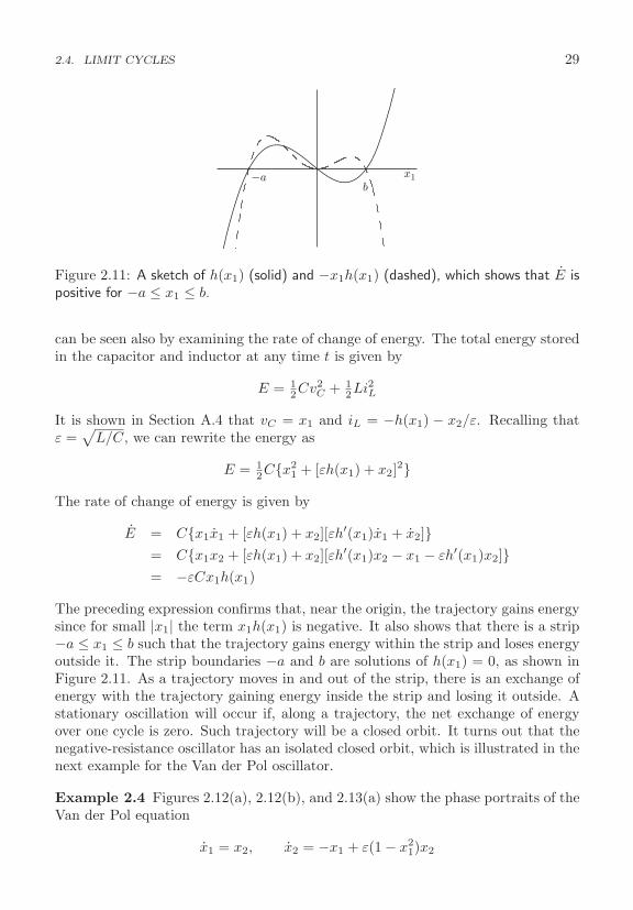
x1−ab
Figure 2.11: A sketch of h(x1) (solid) and −x1h(x1) (dashed), which shows that E ispositive for −a ≤ x1 ≤ b.
can be seen also by examining the rate of change of energy. The total energy storedin the capacitor and inductor at any time t is given by
E = 12Cv2
C + 12Li2L
It is shown in Section A.4 that vC = x1 and iL = −h(x1) − x2/ε. Recalling thatε =√
L/C, we can rewrite the energy as
E = 12C{x2
1 + [εh(x1) + x2]2}
The rate of change of energy is given by
E = C{x1x1 + [εh(x1) + x2][εh′(x1)x1 + x2]}= C{x1x2 + [εh(x1) + x2][εh′(x1)x2 − x1 − εh′(x1)x2]}= −εCx1h(x1)
The preceding expression confirms that, near the origin, the trajectory gains energysince for small |x1| the term x1h(x1) is negative. It also shows that there is a strip−a ≤ x1 ≤ b such that the trajectory gains energy within the strip and loses energyoutside it. The strip boundaries −a and b are solutions of h(x1) = 0, as shown inFigure 2.11. As a trajectory moves in and out of the strip, there is an exchange ofenergy with the trajectory gaining energy inside the strip and losing it outside. Astationary oscillation will occur if, along a trajectory, the net exchange of energyover one cycle is zero. Such trajectory will be a closed orbit. It turns out that thenegative-resistance oscillator has an isolated closed orbit, which is illustrated in thenext example for the Van der Pol oscillator.
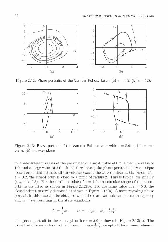
Example 2.4 Figures 2.12(a), 2.12(b), and 2.13(a) show the phase portraits of theVan der Pol equation
x1 = x2, x2 = −x1 + ε(1 − x21)x2
30 CHAPTER 2. TWO-DIMENSIONAL SYSTEMS
−3
−2
−1
0
1
2
3
−2 0 2 4 −2 0 2 4
−2
−1
0
1
2
3
4 x2 x2
x1x1
(a) (b)
Figure 2.12: Phase portraits of the Van der Pol oscillator: (a) ε = 0.2; (b) ε = 1.0.
0 2−3
−2
−1
0
1
2
3
−5 −20 5 10
−5
0
5
10x2
x1
z2
z1
(a) (b)
Figure 2.13: Phase portrait of the Van der Pol oscillator with ε = 5.0: (a) in x1–x2
plane; (b) in z1–z2 plane.
for three different values of the parameter ε: a small value of 0.2, a medium value of1.0, and a large value of 5.0. In all three cases, the phase portraits show a uniqueclosed orbit that attracts all trajectories except the zero solution at the origin. Forε = 0.2, the closed orbit is close to a circle of radius 2. This is typical for small ε(say, ε < 0.3). For the medium value of ε = 1.0, the circular shape of the closedorbit is distorted as shown in Figure 2.12(b). For the large value of ε = 5.0, theclosed orbit is severely distorted as shown in Figure 2.13(a). A more revealing phaseportrait in this case can be obtained when the state variables are chosen as z1 = iLand z2 = vC , resulting in the state equations
z1 =1εz2, z2 = −ε(z1 − z2 + 1
3z32)
The phase portrait in the z1–z2 plane for ε = 5.0 is shown in Figure 2.13(b). Theclosed orbit is very close to the curve z1 = z2 − 1
3z32 , except at the corners, where it
2.5. NUMERICAL CONSTRUCTION OF PHASE PORTRAITS 31
x2 x2
x1x1
(a) (b)
Figure 2.14: (a) A stable limit cycle; (b) an unstable limit cycle.
becomes nearly vertical. The vertical portion of the closed orbit can be viewed asif the closed orbit jumps from one branch of the curve to the other as it reaches thecorner. Oscillations where the jump phenomenon takes place are usually referred toas relaxation oscillations. This phase portrait is typical for large values of ε (say,ε > 3.0). �
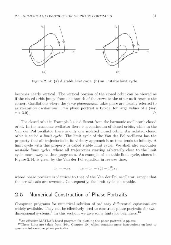
The closed orbit in Example 2.4 is different from the harmonic oscillator’s closedorbit. In the harmonic oscillator there is a continuum of closed orbits, while in theVan der Pol oscillator there is only one isolated closed orbit. An isolated closedorbit is called a limit cycle. The limit cycle of the Van der Pol oscillator has theproperty that all trajectories in its vicinity approach it as time tends to infinity. Alimit cycle with this property is called stable limit cycle. We shall also encounterunstable limit cycles, where all trajectories starting arbitrarily close to the limitcycle move away as time progresses. An example of unstable limit cycle, shown inFigure 2.14, is given by the Van der Pol equation in reverse time,
x1 = −x2, x2 = x1 − ε(1 − x21)x2
whose phase portrait is identical to that of the Van der Pol oscillator, except thatthe arrowheads are reversed. Consequently, the limit cycle is unstable.
2.5 Numerical Construction of Phase Portraits
Computer programs for numerical solution of ordinary differential equations arewidely available. They can be effectively used to construct phase portraits for two-dimensional systems.9 In this section, we give some hints for beginners.10
9An effective MATLAB-based program for plotting the phase portrait is pplane.10These hints are taken from [104, Chapter 10], which contains more instructions on how to
generate informative phase portraits.
32 CHAPTER 2. TWO-DIMENSIONAL SYSTEMS
The first step in constructing the phase portrait is to find all equilibrium pointsand determine the type of isolated ones via linearization.
Drawing trajectories involves three tasks:11
• Selection of a bounding box in the state plane where trajectories are to bedrawn. The box takes the form
x1min ≤ x1 ≤ x1max, x2min ≤ x2 ≤ x2max
• Selection of initial points (conditions) inside the bounding box.
• Calculation of trajectories.
Let us talk first about calculating trajectories. To find the trajectory passingthrough a point x0, solve the equation
x = f(x), x(0) = x0
in forward time (with positive t) and in reverse time (with negative t). Solution inreverse time is equivalent to solution in forward time of the equation
x = −f(x), x(0) = x0
since the change of time variable τ = −t reverses the sign of the right-hand side.The arrowhead on the forward trajectory is placed heading away from x0, while theone on the reverse trajectory is placed heading into x0. Note that solution in reversetime is the only way we can get a good portrait in the neighborhood of unstablefocus, unstable node, or unstable limit cycle. Trajectories are continued until theyget out of the bounding box. If processing time is a concern, you may want to adda stopping criterion when trajectories converge to an equilibrium point.
The bounding box should be selected so that all essential qualitative featuresare displayed. Since some of these features will not be known a priori, we may haveto adjust the bounding box interactively. However, our initial choice should makeuse of all prior information. For example, the box should include all equilibriumpoints. Care should be exercised when a trajectory travels out of bounds, for sucha trajectory is either unbounded or is attracted to a stable limit cycle.
The simplest approach to select initial points is to place them uniformly on a gridthroughout the bounding box. However, an evenly spaced set of initial conditionsrarely yields an evenly spaced set of trajectories. A better approach is to select theinitial points interactively after plotting the already calculated trajectories. Sincemost computer programs have sophisticated plotting tools, this approach should bequite feasible.
For a saddle point, we can use linearization to generate the stable and unstabletrajectories. This is useful because, as we saw in Examples 2.2 and 2.3, the stable
11A fourth task that we left out is placing arrowheads on the trajectory. For the purpose of thistextbook, it can be conveniently done manually.
2.6. EXERCISES 33
trajectories of a saddle define a separatrix. Let the eigenvalues of the linearizationbe λ1 > 0 > λ2 and the corresponding eigenvectors be v1 and v2. The stable andunstable trajectories of the nonlinear saddle will be tangent to the stable eigenvectorv2 and the unstable eigenvector v1, respectively, as they approach the equilibriumpoint p. Therefore, the two unstable trajectories can be generated from the initialpoints x0 = p ± αv1, where α is a small positive number. Similarly, the two stabletrajectories can be generated from the initial points x0 = p±αv2. The major partsof the unstable trajectories will be generated by solution in forward time, while themajor parts of the stable ones will be generated by solution in reverse time.
2.6 Exercises
2.1 For each of the following systems,
(a) Find all equilibrium points and determine their types.
(b) Construct and discuss the phase portrait.
(1) x1 = −x31 + x2, x2 = x1 − x3
2
(2) x1 = x2, x2 = x1 − x2 − 0.5(x1 + x2)2
(3) x1 = x2, x2 = 2x1 + 3x21 + x3
1 − x2
(4) x1 = −x2 + 14x3
2, x2 = 4x1 − 2x2
(5) x1 = x2, x2 = −x1 + x2(1 − x21 + 0.1x4
1)
(6) x1 = −x1 + 2x2 + x1x2 + x22, x2 = −x1 − x2
1 − x1x2
(7) x1 = x2, x2 = −(x1 + x2)/(x1 + 2) (defined over the set {x1 > −2})(8) x1 = −x2, x2 = 2x1 + 3x2 + 2 sat(−3x2)
(9) x1 = x2, x2 = −x1 + 116x3
1 + x2 − 13x3
2
2.2 Consider the tunnel-diode circuit of Example 2.2. Keep all parameters thesame except u. Construct and discuss the phase portrait when
(a) u = 0.4;
(b) u = 2.
2.3 Consider the biochemical reactor (A.19) with ν defined by (A.20). Let α = 23,β = 0.39, and γ = 0.57. Construct and discuss the phase portrait in the region{x1 ≥ 0, x2 ≥ 0} when
(a) u = 0.5;
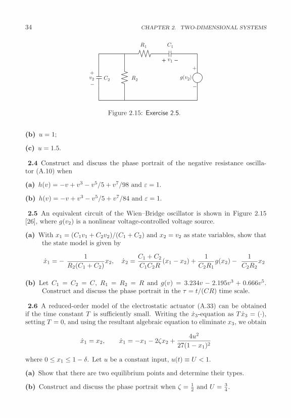
34 CHAPTER 2. TWO-DIMENSIONAL SYSTEMS
C2
C1R1
R2v2
+ −v1
++ −
−
+
−g(v2)
Figure 2.15: Exercise 2.5.
(b) u = 1;
(c) u = 1.5.
2.4 Construct and discuss the phase portrait of the negative resistance oscilla-tor (A.10) when
(a) h(v) = −v + v3 − v5/5 + v7/98 and ε = 1.
(b) h(v) = −v + v3 − v5/5 + v7/84 and ε = 1.
2.5 An equivalent circuit of the Wien–Bridge oscillator is shown in Figure 2.15[26], where g(v2) is a nonlinear voltage-controlled voltage source.
(a) With x1 = (C1v1 + C2v2)/(C1 + C2) and x2 = v2 as state variables, show thatthe state model is given by
x1 = − 1R2(C1 + C2)
x2, x2 =C1 + C2
C1C2R(x1 − x2) +
1C2R1
g(x2) − 1C2R2
x2
(b) Let C1 = C2 = C, R1 = R2 = R and g(v) = 3.234v − 2.195v3 + 0.666v5.Construct and discuss the phase portrait in the τ = t/(CR) time scale.
2.6 A reduced-order model of the electrostatic actuator (A.33) can be obtainedif the time constant T is sufficiently small. Writing the x3-equation as T x3 = (·),setting T = 0, and using the resultant algebraic equation to eliminate x3, we obtain
x1 = x2, x1 = −x1 − 2ζx2 +4u2
27(1 − x1)2
where 0 ≤ x1 ≤ 1 − δ. Let u be a constant input, u(t) ≡ U < 1.
(a) Show that there are two equilibrium points and determine their types.
(b) Construct and discuss the phase portrait when ζ = 12 and U = 3
4 .
2.6. EXERCISES 35
2.7 Consider the inverted pendulum equation (A.47) with a = 1.
(a) With u = 0, find all equilibrium points and determine their types.
(b) The energy E = 1 + cos x1 + 12x2
2 is defined such that E = 2 at the upwardequilibrium position (0, 0) and E = 0 at the downward one (π, 0). To swingup the pendulum we need to pump up the energy. Show that the controlu = k(2 − E)x2 cos(x1), with k > 0, will make E > 0 whenever E < 2 andx2 cos x1 �= 0.
(c) Consider the closed-loop system under the foregoing control. Construct anddiscuss the phase portrait when k = 0.1.
2.8 Consider the system
x1 = x2, x2 = −0.5x1 + 1.5x2 + 0.5u
Construct and discuss the phase portrait for u = 0, the feedback control u =0.9x1 − 3.2x2, and the constrained feedback control u = sat(0.9x1 − 3.2x2).
2.9 Construct and discuss the phase portrait of the system
x1 = x2, x2 = x1 − x2 + μ sat(−2x1 + 1
2x2
)for each of the values μ = 0.25, 1, and 3.
2.10 The elementary processing units in the central nervous system are the neu-rons. The FitzHugh-Nagumo model [49] is a dimensionless model that attempts tocapture the dynamics of a single neuron. It is given by
u = u − 13u3 − w + I, w = ε(b0 + b1u − w)
where u, w, and I ≥ 0 are the membrane voltage, recovery variable, and appliedcurrent, respectively. The constants ε, b0 and b1 are positive.
(a) Find all equilibrium points and determine their types when b1 > 1.
(b) Repeat part (a) when b1 < 1.
(c) Let ε = 0.1, b0 = 2 and b1 = 1.5. For each of the values I = 0 and I = 2,construct the phase portrait and discuss the qualitative behavior of the system.
(d) Repeat (c) with b1 = 0.5.
2.11 Consider the magnetic levitation system (A.29) under the feedback controlu = −1 + sat
(12 − x1 − x2
).
(a) Find all equilibrium points and determine their types when c = 1 and whenc �= 1 but |(1 − c)/c| < 1.

36 CHAPTER 2. TWO-DIMENSIONAL SYSTEMS
(b) Construct and discuss the phase portrait when b = 0.01 and c = 23 , taking into
consideration the constraint 0 ≤ x1 ≤ 5.
2.12 [77] Consider the nonlinear system
x1 = x2, x2 = 0.1x32 + u
under the feedback control u = −γ2x1 − γx2, with γ > 0. The linearization at theorigin has the eigenvalues (γ/2)(−1± j
√3), so the response of the linearization can
be made faster by increasing γ. To study the effect of increasing γ on the behaviorof the nonlinear system, it is convenient to apply the change of variables z1 =
√γx1,
z2 = x2/√
γ, and τ = γt.
(a) Show that the transformed state equation in the τ time scale is given by
z1 = z2, z2 = −z1 − z2 + 0.1z32
(b) Construct and discuss the phase portrait in the z1–z2 plane.
(c) Discuss the effect of increasing γ on the phase portrait in the x1–x2 plane.
Chapter 3
Stability of Equilibrium Points
Stability theory plays a central role in systems theory and engineering. There aredifferent kinds of stability problems that arise in the study of dynamical systems.This chapter is concerned with stability of equilibrium points for time-invariant sys-tems. In later chapters, we shall deal with time-varying systems and see other kindsof stability, such as input-to-state stability and input–output stability. An equilib-rium point is stable if all solutions starting at nearby points stay nearby; otherwise,it is unstable. It is asymptotically stable if all solutions starting at nearby pointsnot only stay nearby, but also tend to the equilibrium point as time approachesinfinity. These notions are made precise in Section 3.1. In the same section wesee how to study stability of equilibrium points for linear systems and scalar (orone-dimensional) nonlinear systems. In Section 3.2 we use linearization to study thestability of equilibrium points of nonlinear systems. Lyapunov’s method is intro-duced in Section 3.3 and an extension of the basic theory, known as the invarianceprinciple, is covered in Section 3.4. Sections 3.5 and 3.6 elaborate on two conceptsthat are introduced in Section 3.1, namely, exponential stability and the region ofattraction. The chapter ends in Section 3.7 with two converse Lyapunov theorems,one for asymptotic stability and the other for its special case of exponential stability.
3.1 Basic Concepts
Consider the n-dimensional time-invariant system
x = f(x) (3.1)
where f is locally Lipschitz over a domain D ⊂ Rn. Suppose x ∈ D is an equilibriumpoint of (3.1); that is, f(x) = 0. Our goal is to characterize and study the stabilityof x. For convenience, we state all definitions and theorems for the case when theequilibrium point is at the origin of Rn; that is, x = 0. There is no loss of generalityin doing so because any equilibrium point can be shifted to the origin via a change
37

38 CHAPTER 3. STABILITY OF EQUILIBRIUM POINTS
of variables. Suppose x �= 0 and consider the change of variables y = x − x. Thederivative of y is given by
y = x = f(x) = f(y + x) def= g(y), where g(0) = 0
In the new variable y, the system has an equilibrium point at the origin. Therefore,without loss of generality, we assume that f(x) satisfies f(0) = 0 and study thestability of the origin x = 0.
Definition 3.1 Let f(x) be a locally Lipschitz function defined over a domain D ⊂Rn, which contains the origin, and f(0) = 0. The equilibrium point x = 0 ofx = f(x) is
• stable if for each ε > 0 there is δ > 0 (dependent on ε) such that
‖x(0)‖ < δ ⇒ ‖x(t)‖ < ε, ∀ t ≥ 0
• unstable if it is not stable.
• asymptotically stable if it is stable and δ can be chosen such that
‖x(0)‖ < δ ⇒ limt→∞x(t) = 0
The ε–δ requirement for stability takes a challenge-answer form. To demonstratethat the origin is stable, then, for any value of ε that a challenger may care to desig-nate, we must produce a value of δ, possibly dependent on ε, such that a trajectorystarting in a δ neighborhood of the origin will never leave the ε neighborhood. Thethree types of stability properties can be illustrated by the pendulum example ofSection A.1. The pendulum equation
x1 = x2, x2 = − sin x1 − bx2
has equilibrium points at (0, 0) and (π, 0). Neglecting friction, by setting b = 0,we have seen in Chapter 2 (Figure 2.2) that trajectories in the neighborhood ofthe origin are closed orbits. Therefore, by starting sufficiently close to the origin,trajectories can be guaranteed to stay within any specified ball centered at theorigin. Hence, the ε–δ requirement for stability is satisfied. The origin, however, isnot asymptotically stable since trajectories do not tend to it eventually. Instead,they remain in their closed orbits. When friction is taken into consideration (b > 0),the origin becomes a stable focus. Inspection of the phase portrait of a stable focusshows that the ε–δ requirement for stability is satisfied. In addition, trajectoriesstarting close to the equilibrium point tend to it as time tends to infinity. Theequilibrium point at x1 = π is a saddle. Clearly the ε–δ requirement cannot besatisfied since, for any ε > 0, there is always a trajectory that will leave the ball{‖x − x‖ ≤ ε} even when x(0) is arbitrarily close to the equilibrium point x.

3.1. BASIC CONCEPTS 39
f(x) f(x) f(x)
x x x
Figure 3.1: Examples of f(x) for which the origin of x = f(x) is unstable.
Having defined stability and asymptotic stability of equilibrium points, our tasknow is to find ways to determine stability. The approach we used in the pendulumexample relied on our knowledge of the phase portrait. Trying to generalize thisapproach amounts to actually finding all solutions of the state equation, whichmay be difficult or even impossible. Lyapunov’s method provides us with a toolto investigate stability of equilibrium points without the need to solve the stateequation. There are, however, two special cases where we can determine stabilitywithout Lyapunov’ method, namely, scalar and linear systems.
In the scalar (one-dimensional) case, the behavior of x(t) in the neighborhoodof the origin can be determined by examining the sign of f(x). In particular, theε–δ requirement for stability is violated if xf(x) > 0 on either side of the originx = 0 because in this case a trajectory starting arbitrarily close to the origin willhave to move away from it and cannot be maintained in an ε neighborhood bychoosing δ small enough. Examples of such situation are shown in Figure 3.1.Consequently, a necessary condition for the origin to be stable is to have xf(x) ≤ 0in some neighborhood of the origin. It is not hard to see that this condition is alsosufficient. For asymptotic stability, we need to show that there is a neighborhood ofthe origin such that trajectories starting in this neighborhood will converge to zeroas time tends to infinity. Clearly, this will not be the case if f(x) is identically zeroon either side of the origin, as in the examples shown in Figure 3.2. Again, it is nothard to see that the origin will be asymptotically stable if and only if xf(x) < 0in some neighborhood of the origin; examples of functions satisfying this conditionare shown in Figure 3.3. Let us note an important difference between the twoexamples of Figure 3.3. For the system whose right-hand side function is shown inFigure 3.3(a), limt→∞ x(t) = 0 holds only for initial states in the set {−a < x < b},while for that of Figure 3.3(b) the limit holds for all initial states. In the first case,the set {−a < x < b} is said to be the region of attraction, while in the second casethe origin is said to be globally asymptotically stable. These notions are definednext for n-dimensional systems.
Definition 3.2 Let the origin be an asymptotically stable equilibrium point of thesystem x = f(x), where f is a locally Lipschitz function defined over a domainD ⊂ Rn that contains the origin. Then,
• the region of attraction of the origin (also called region of asymptotic stability,
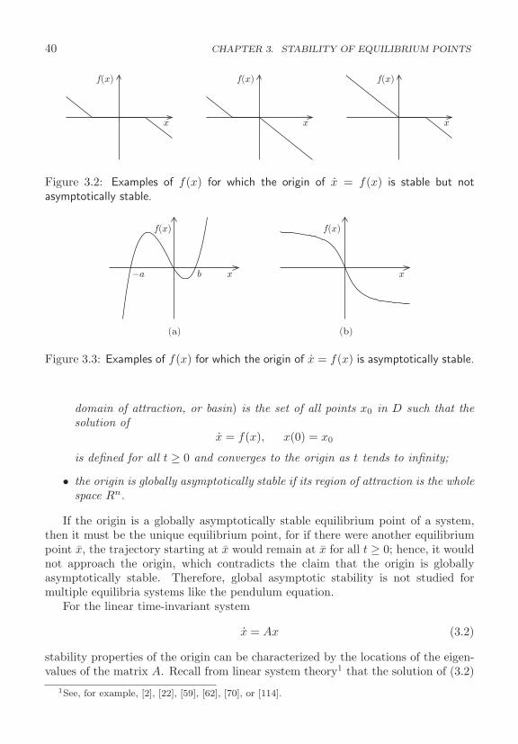
40 CHAPTER 3. STABILITY OF EQUILIBRIUM POINTS
f(x) f(x) f(x)
x x x
Figure 3.2: Examples of f(x) for which the origin of x = f(x) is stable but notasymptotically stable.
f(x) f(x)
xx−a b
(a) (b)
Figure 3.3: Examples of f(x) for which the origin of x = f(x) is asymptotically stable.
domain of attraction, or basin) is the set of all points x0 in D such that thesolution of
x = f(x), x(0) = x0
is defined for all t ≥ 0 and converges to the origin as t tends to infinity;
• the origin is globally asymptotically stable if its region of attraction is the wholespace Rn.
If the origin is a globally asymptotically stable equilibrium point of a system,then it must be the unique equilibrium point, for if there were another equilibriumpoint x, the trajectory starting at x would remain at x for all t ≥ 0; hence, it wouldnot approach the origin, which contradicts the claim that the origin is globallyasymptotically stable. Therefore, global asymptotic stability is not studied formultiple equilibria systems like the pendulum equation.
For the linear time-invariant system
x = Ax (3.2)
stability properties of the origin can be characterized by the locations of the eigen-values of the matrix A. Recall from linear system theory1 that the solution of (3.2)
1See, for example, [2], [22], [59], [62], [70], or [114].

3.1. BASIC CONCEPTS 41
for a given initial state x(0) is given by
x(t) = exp(At)x(0) (3.3)
and that for any matrix A there is a nonsingular matrix P (possibly complex) thattransforms A into its Jordan form; that is,
P−1AP = J = block diag[J1, J2, . . . , Jr]
where Ji is a Jordan block associated with the eigenvalue λi of A. A Jordan blockof order one takes the form Ji = λi, while a Jordan block of order m > 1 takes theform
Ji =
⎡⎢⎢⎢⎢⎢⎢⎢⎢⎢⎣
λi 1 0 . . . . . . 00 λi 1 0 . . . 0...
. . ....
.... . . 0
.... . . 1
0 . . . . . . . . . 0 λi
⎤⎥⎥⎥⎥⎥⎥⎥⎥⎥⎦
m×m
Therefore,
exp(At) = P exp(Jt)P−1 =r∑
i=1
mi∑k=1
tk−1 exp(λit)Rik (3.4)
where mi is the order of the Jordan block Ji. If an n × n matrix A has a repeatedeigenvalue λi of algebraic multiplicity qi,2 then the Jordan blocks associated with λi
have order one if and only if rank(A−λiI) = n−qi. The next theorem characterizesthe stability properties of the origin.
Theorem 3.1 The equilibrium point x = 0 of x = Ax is stable if and only if alleigenvalues of A satisfy Re[λi] ≤ 0 and for every eigenvalue with Re[λi] = 0 andalgebraic multiplicity qi ≥ 2, rank(A − λiI) = n − qi, where n is the dimension ofx. The equilibrium point x = 0 is globally asymptotically stable if and only if alleigenvalues of A satisfy Re[λi] < 0. �
Proof: From (3.3) we can see that the origin is stable if and only if exp(At) is abounded function of t for all t ≥ 0. If one of the eigenvalues of A has Re[λi] > 0, thecorresponding exponential term exp(λit) in (3.4) will grow unbounded as t → ∞.Therefore, we must restrict the eigenvalues to have Re[λi] ≤ 0. However, thoseeigenvalues with Re[λi] = 0 (if any) could give rise to unbounded terms if the orderof an associated Jordan block is higher than one, due to the term tk−1 in (3.4).Therefore, we must restrict eigenvalues with zero real parts to have Jordan blocksof order one, which is equivalent to the rank condition rank(A − λiI) = n − qi.Thus, we conclude that the condition for stability is a necessary one. It is clear that
2Equivalently, qi is the multiplicity of λi as a zero of det(λI − A).

42 CHAPTER 3. STABILITY OF EQUILIBRIUM POINTS
+
(a) (b)
Figure 3.4: (a) Series connection; (b) parallel connection.
the condition is also sufficient to ensure that exp(At) is bounded. For asymptoticstability of the origin, exp(At) must approach 0 as t → ∞. From (3.4), this is thecase if and only if Re[λi] < 0, ∀ i. Since x(t) depends linearly on the initial statex(0), asymptotic stability of the origin is global. �
The proof shows, mathematically, why repeated eigenvalues on the imaginaryaxis must satisfy the rank condition rank(A − λiI) = n − qi. The next examplesheds some light on the physical meaning of this requirement.
Example 3.1 Figure 3.4 shows a series connection and a parallel connection of twoidentical systems. Each system is represented by the state model
x =[
0 1−1 0
]x +[
01
]u, y =
[1 0
]x
where u and y are the input and output, respectively. Let As and Ap be the matricesof the series and parallel connections, when modeled in the form (3.2) (no drivinginputs). Then
Ap =
⎡⎢⎢⎣
0 1 0 0−1 0 0 0
0 0 0 10 0 −1 0
⎤⎥⎥⎦ and As =
⎡⎢⎢⎣
0 1 0 0−1 0 0 0
0 0 0 11 0 −1 0
⎤⎥⎥⎦
The matrices Ap and As have the same eigenvalues on the imaginary axis, ±j,with algebraic multiplicity qi = 2, where j =
√−1. It can be easily checked thatrank(Ap−jI) = 2 = n−qi, while rank(As−jI) = 3 �= n−qi. Thus, by Theorem 3.1,the origin of the parallel connection is stable, while the origin of the series connectionis unstable. To physically see the difference between the two cases, notice that inthe parallel connection, nonzero initial conditions produce sinusoidal oscillationsof frequency 1 rad/sec, which are bounded functions of time. The sum of thesesinusoidal signals remains bounded. On the other hand, nonzero initial conditionsin the first component of the series connection produce a sinusoidal oscillation offrequency 1 rad/sec, which acts as a driving input to the second component. Since
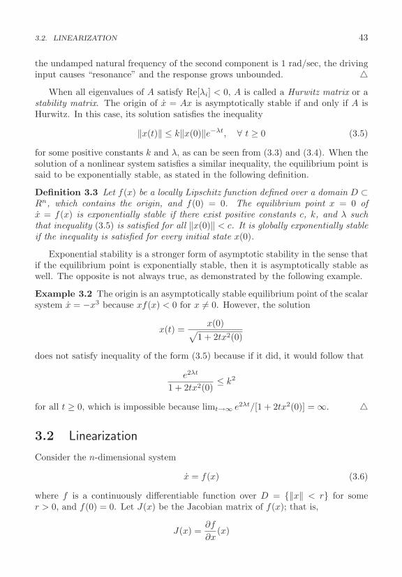
3.2. LINEARIZATION 43
the undamped natural frequency of the second component is 1 rad/sec, the drivinginput causes “resonance” and the response grows unbounded. �
When all eigenvalues of A satisfy Re[λi] < 0, A is called a Hurwitz matrix or astability matrix. The origin of x = Ax is asymptotically stable if and only if A isHurwitz. In this case, its solution satisfies the inequality
‖x(t)‖ ≤ k‖x(0)‖e−λt, ∀ t ≥ 0 (3.5)
for some positive constants k and λ, as can be seen from (3.3) and (3.4). When thesolution of a nonlinear system satisfies a similar inequality, the equilibrium point issaid to be exponentially stable, as stated in the following definition.
Definition 3.3 Let f(x) be a locally Lipschitz function defined over a domain D ⊂Rn, which contains the origin, and f(0) = 0. The equilibrium point x = 0 ofx = f(x) is exponentially stable if there exist positive constants c, k, and λ suchthat inequality (3.5) is satisfied for all ‖x(0)‖ < c. It is globally exponentially stableif the inequality is satisfied for every initial state x(0).
Exponential stability is a stronger form of asymptotic stability in the sense thatif the equilibrium point is exponentially stable, then it is asymptotically stable aswell. The opposite is not always true, as demonstrated by the following example.
Example 3.2 The origin is an asymptotically stable equilibrium point of the scalarsystem x = −x3 because xf(x) < 0 for x �= 0. However, the solution
x(t) =x(0)√
1 + 2tx2(0)
does not satisfy inequality of the form (3.5) because if it did, it would follow that
e2λt
1 + 2tx2(0)≤ k2
for all t ≥ 0, which is impossible because limt→∞ e2λt/[1 + 2tx2(0)] = ∞. �
3.2 Linearization
Consider the n-dimensional system
x = f(x) (3.6)
where f is a continuously differentiable function over D = {‖x‖ < r} for somer > 0, and f(0) = 0. Let J(x) be the Jacobian matrix of f(x); that is,
J(x) =∂f
∂x(x)
44 CHAPTER 3. STABILITY OF EQUILIBRIUM POINTS
By (B.6) and f(0) = 0, we have
f(x) =∫ 1
0
J(σx) dσ x
Let A = J(0). By adding and subtracting Ax to the right-hand side of the foregoingequation, we obtain
f(x) = [A + G(x)]x, where G(x) =∫ 1
0
[J(σx) − J(0)] dσ
By continuity of J(x), we see that G(x) → 0 as x → 0. This suggests that in a smallneighborhood of the origin we can approximate the nonlinear system x = f(x) by itslinearization about the origin x = Ax. The next theorem spells out conditions underwhich we can draw conclusions about the stability of the origin as an equilibriumpoint for the nonlinear system by investigating its stability as an equilibrium pointfor the linear system. The theorem is known as Lyapunov’s indirect method.3
Theorem 3.2 Let x = 0 be an equilibrium point for the nonlinear system x = f(x),where f is continuously differentiable in a neighborhood of the origin. Let
A =∂f
∂x(x)∣∣∣∣x=0
and denote its eigenvalues by λ1 to λn. Then,
1. The origin is exponentially stable if and only if Re[λi] < 0 for all eigenvalues.
2. The origin is unstable if Re[λi] > 0 for one or more of the eigenvalues.
�
Theorem 3.2 provides us with a simple procedure for determining the stability ofan equilibrium point by testing the eigenvalues of the Jacobian at that point. Thetheorem, however, does not say anything about the case when Re[λi] ≤ 0 for all i,with Re[λi] = 0 for some i. In this case, linearization fails to determine the stabilityof the equilibrium point, although we can say for sure that if the equilibrium pointturns out to be asymptotically stable, it will not be exponentially stable becausethe condition for exponential stability is both necessary and sufficient.
Example 3.3 Consider the scalar system x = ax3. Linearizing the system aboutthe origin yields
A =∂f
∂x
∣∣∣∣x=0
= 3ax2∣∣x=0
= 0
3See [74, Theorems 4.7 and 4.15] for the proof of Theorem 3.2. For the first item of the theorem,a proof of the sufficiency part is given in Section 3.5 while a proof of the necessity part is given inSection 3.7.

3.3. LYAPUNOV’S METHOD 45
There is one eigenvalue that lies on the imaginary axis. Hence, linearization failsto determine the stability of the origin. This failure is genuine in the sense that theorigin could be asymptotically stable, stable, or unstable, depending on the valueof the parameter a. If a < 0, the origin is asymptotically stable as can be seen fromthe condition xf(x) = ax4 < 0 for x �= 0. If a = 0, the system is linear and theorigin is stable according to Theorem 3.1. If a > 0, the origin is unstable as can beseen from the condition xf(x) = ax4 > 0 for x �= 0. Notice that when a < 0, theorigin is not exponentially stable, as we saw in Example 3.2.4 �Example 3.4 The pendulum equation
x1 = x2, x2 = − sin x1 − bx2
has equilibrium points at (0, 0) and (π, 0). The Jacobian matrix is
∂f
∂x=
⎡⎣ ∂f1
∂x1
∂f1∂x2
∂f2∂x1
∂f2∂x2
⎤⎦ =
⎡⎣ 0 1
− cos x1 −b
⎤⎦
To determine the stability of the origin, we evaluate the Jacobian at x = 0:
A =∂f
∂x
∣∣∣∣x=0
=[
0 1−1 −b
]The eigenvalues of A are λ1,2 = − 1
2b ± 12
√b2 − 4. For all b > 0, the eigenvalues
satisfy Re[λi] < 0. Consequently, the equilibrium point at the origin is exponentiallystable. In the absence of friction (b = 0), both eigenvalues are on the imaginaryaxis. Thus, we cannot determine the stability of the origin through linearization.We know from the phase portrait (Figure 2.2) that, in this case, the origin is acenter; hence, it is a stable equilibrium point. To determine the stability of theequilibrium point at (π, 0), we evaluate the Jacobian at that point. This is equivalentto performing a change of variables z1 = x1 − π, z2 = x2 to shift the equilibriumpoint to the origin and then evaluating the Jacobian [∂f/∂z] at z = 0:
A =∂f
∂x
∣∣∣∣x1=π,x2=0
=[
0 11 −b
]
The eigenvalues of A are λ1,2 = − 12b ± 1
2
√b2 + 4. For all b ≥ 0, there is one
eigenvalue with Re[λi] > 0. Hence, the equilibrium point at (π, 0) is unstable. �
3.3 Lyapunov’s Method
Reconsider the pendulum equation
x1 = x2, x2 = − sin x1 − bx2
4While the example dealt with the case a = −1, its conclusion extends to any a < 0 by changingthe time variable from t to τ = −at, transforming x = ax3 to dx/dτ = −x3.
46 CHAPTER 3. STABILITY OF EQUILIBRIUM POINTS
where b ≥ 0. Using phase portraits and/or linearization, we have argued in theprevious two sections that the origin is a stable equilibrium point when b = 0 andasymptotically stable when b > 0. These conclusions can also be reached usingenergy concepts. Let us define the energy of the pendulum E(x) as the sum ofits potential and kinetic energies, with the reference of the potential energy chosensuch that E(0) = 0; that is,
E(x) =∫ x1
0
sin y dy + 12x2
2 = (1 − cos x1) + 12x2
2
When friction is neglected (b = 0), the system is conservative; that is, there is nodissipation of energy. Hence, E = constant during the motion of the system or, inother words, dE/dt = 0 along the trajectories of the system. Since E(x) = c formsa closed contour around x = 0 for small c, we can again arrive at the conclusionthat x = 0 is a stable equilibrium point. When friction is accounted for (b > 0),energy will dissipate during the motion of the system, that is, dE/dt ≤ 0 along thetrajectories of the system. Due to friction, E cannot remain constant indefinitelywhile the system is in motion. Hence, it keeps decreasing until it eventually reacheszero, showing that the trajectory tends to x = 0 as t tends to ∞. Thus, by examiningthe derivative of E along the trajectories of the system, it is possible to determinethe stability of the equilibrium point. In 1892, Lyapunov showed that certain otherfunctions could be used instead of energy to determine stability of an equilibriumpoint.5 Let V (x) be a continuously differentiable real-valued function defined in adomain D ⊂ Rn that contains the origin. The derivative of V along the trajectoriesof x = f(x), denoted by V (x), is given by
V (x) =n∑
i=1
∂V
∂xixi =
n∑i=1
∂V
∂xifi(x)
=[
∂V∂x1
, ∂V∂x2
, . . . , ∂V∂xn
]⎡⎢⎢⎢⎣
f1(x)f2(x)
...fn(x)
⎤⎥⎥⎥⎦ =
∂V
∂xf(x)
The derivative of V along the trajectories of a system is dependent on the system’sequation. Hence, V (x) will be different for different systems. If φ(t;x) is the solutionof x = f(x) that starts at initial state x at time t = 0, then
V (x) =d
dtV (φ(t;x))
∣∣∣∣t=0
Therefore, if V (x) is negative, V will decrease along the solution of x = f(x). Thisobservation leads to Lyapunov’s stability theorem, given next.
5Classical references on Lyapunov stability include [54, 78, 111, 152, 156].

3.3. LYAPUNOV’S METHOD 47
Br
Bδ
D
βΩ
Figure 3.5: Geometric representation of sets in the proof of Theorem 3.3.
Theorem 3.3 Let f(x) be a locally Lipschitz function defined over a domain D ⊂Rn, which contains the origin, and f(0) = 0. Let V (x) be a continuously differen-tiable function defined over D such that
V (0) = 0 and V (x) > 0 for all x ∈ D with x �= 0 (3.7)
V (x) ≤ 0 for all x ∈ D (3.8)
Then, the origin is a stable equilibrium point of x = f(x). Moreover, if
V (x) < 0 for all x ∈ D with x �= 0 (3.9)
then origin is asymptotically stable. Furthermore, if D = Rn, (3.7) and (3.9) holdfor all x �= 0, and
‖x‖ → ∞ ⇒ V (x) → ∞ (3.10)
then the origin is globally asymptotically stable. �
Proof: Given ε > 0, choose r ∈ (0, ε] such that Br = {‖x‖ ≤ r} ⊂ D.6 Letα = min‖x‖=r V (x). By (3.7), α > 0 . Take β ∈ (0, α) and let
Ωβ = {x ∈ Br | V (x) ≤ β}
Then, Ωβ is in the interior of Br.7 (See Figure 3.5.) The set Ωβ has the property
6The definition of stability should hold for any ε > 0, but the analysis has to be limited to thedomain D. Because r ≤ ε, if we show that ‖x(t)‖ ≤ r we will have ‖x(t)‖ ≤ ε.
7This fact can be shown by contradiction. Suppose Ωβ is not in the interior of Br, then thereis a point p ∈ Ωβ that lies on the boundary of Br. At this point, V (p) ≥ α > β, but for allx ∈ Ωβ , V (x) ≤ β, which is a contradiction.
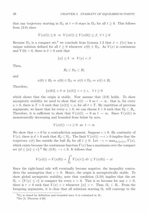
48 CHAPTER 3. STABILITY OF EQUILIBRIUM POINTS
that any trajectory starting in Ωβ at t = 0 stays in Ωβ for all t ≥ 0. This followsfrom (3.8) since
V (x(t)) ≤ 0 ⇒ V (x(t)) ≤ V (x(0)) ≤ β, ∀ t ≥ 0
Because Ωβ is a compact set,8 we conclude from Lemma 1.3 that x = f(x) has aunique solution defined for all t ≥ 0 whenever x(0) ∈ Ωβ . As V (x) is continuousand V (0) = 0, there is δ > 0 such that
‖x‖ ≤ δ ⇒ V (x) < β
Then,Bδ ⊂ Ωβ ⊂ Br
andx(0) ∈ Bδ ⇒ x(0) ∈ Ωβ ⇒ x(t) ∈ Ωβ ⇒ x(t) ∈ Br
Therefore,‖x(0)‖ < δ ⇒ ‖x(t)‖ < r ≤ ε, ∀ t ≥ 0
which shows that the origin is stable. Now assume that (3.9) holds. To showasymptotic stability we need to show that x(t) → 0 as t → ∞. that is, for everya > 0, there is T > 0 such that ‖x(t)‖ < a, for all t > T . By repetition of previousarguments, we know that for every a > 0, we can choose b > 0 such that Ωb ⊂ Ba.Therefore, it is sufficient to show that V (x(t)) → 0 as t → ∞. Since V (x(t)) ismonotonically decreasing and bounded from below by zero,
V (x(t)) → c ≥ 0 as t → ∞
We show that c = 0 by a contradiction argument. Suppose c > 0. By continuity ofV (x), there is d > 0 such that Bd ⊂ Ωc. The limit V (x(t)) → c > 0 implies that thetrajectory x(t) lies outside the ball Bd for all t ≥ 0. Let −γ = maxd≤‖x‖≤r V (x),which exists because the continuous function V (x) has a maximum over the compactset {d ≤ ‖x‖ ≤ r}.9 By (3.9), −γ < 0. It follows that
V (x(t)) = V (x(0)) +∫ t
0
V (x(τ)) dτ ≤ V (x(0)) − γt
Since the right-hand side will eventually become negative, the inequality contra-dicts the assumption that c > 0. Hence, the origin is asymptotically stable. Toshow global asymptotic stability, note that condition (3.10) implies that the setΩc = {V (x) ≤ c} is compact for every c > 0. This is so because for any c > 0,there is r > 0 such that V (x) > c whenever ‖x‖ > r. Thus, Ωc ⊂ Br. From theforegoing arguments, it is clear that all solutions starting Ωc will converge to the
8Ωβ is closed by definition and bounded since it is contained in Br.9See [3, Theorem 4-20].
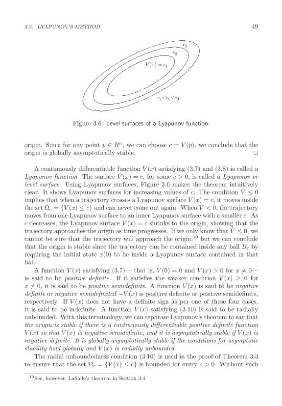
3.3. LYAPUNOV’S METHOD 49
c2
c3
c1<c2< c3
V (x) = c1
Figure 3.6: Level surfaces of a Lyapunov function.
origin. Since for any point p ∈ Rn, we can choose c = V (p), we conclude that theorigin is globally asymptotically stable. �
A continuously differentiable function V (x) satisfying (3.7) and (3.8) is called aLyapunov function. The surface V (x) = c, for some c > 0, is called a Lyapunov orlevel surface. Using Lyapunov surfaces, Figure 3.6 makes the theorem intuitivelyclear. It shows Lyapunov surfaces for increasing values of c. The condition V ≤ 0implies that when a trajectory crosses a Lyapunov surface V (x) = c, it moves insidethe set Ωc = {V (x) ≤ c} and can never come out again. When V < 0, the trajectorymoves from one Lyapunov surface to an inner Lyapunov surface with a smaller c. Asc decreases, the Lyapunov surface V (x) = c shrinks to the origin, showing that thetrajectory approaches the origin as time progresses. If we only know that V ≤ 0, wecannot be sure that the trajectory will approach the origin,10 but we can concludethat the origin is stable since the trajectory can be contained inside any ball Bε byrequiring the initial state x(0) to lie inside a Lyapunov surface contained in thatball.
A function V (x) satisfying (3.7)— that is, V (0) = 0 and V (x) > 0 for x �= 0—is said to be positive definite. If it satisfies the weaker condition V (x) ≥ 0 forx �= 0, it is said to be positive semidefinite. A function V (x) is said to be negativedefinite or negative semidefiniteif −V (x) is positive definite or positive semidefinite,respectively. If V (x) does not have a definite sign as per one of these four cases,it is said to be indefinite. A function V (x) satisfying (3.10) is said to be radiallyunbounded. With this terminology, we can rephrase Lyapunov’s theorem to say thatthe origin is stable if there is a continuously differentiable positive definite functionV (x) so that V (x) is negative semidefinite, and it is asymptotically stable if V (x) isnegative definite. It is globally asymptotically stable if the conditions for asymptoticstability hold globally and V (x) is radially unbounded.
The radial unboundedness condition (3.10) is used in the proof of Theorem 3.3to ensure that the set Ωc = {V (x) ≤ c} is bounded for every c > 0. Without such
10See, however, LaSalle’s theorem in Section 3.4
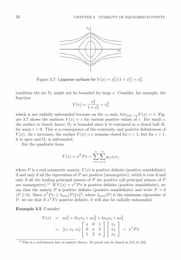
50 CHAPTER 3. STABILITY OF EQUILIBRIUM POINTS
x2
x1
Figure 3.7: Lyapunov surfaces for V (x) = x21/(1 + x2
1) + x22.
condition the set Ωc might not be bounded for large c. Consider, for example, thefunction
V (x) =x2
1
1 + x21
+ x22
which is not radially unbounded because on the x1-axis, lim‖x‖→∞V (x) = 1. Fig-ure 3.7 shows the surfaces V (x) = c for various positive values of c. For small c,the surface is closed; hence, Ωc is bounded since it is contained in a closed ball Br
for some r > 0. This is a consequence of the continuity and positive definiteness ofV (x). As c increases, the surface V (x) = c remains closed for c < 1, but for c > 1,it is open and Ωc is unbounded.
For the quadratic form
V (x) = xT Px =n∑
i=1
n∑j=1
pijxixj
where P is a real symmetric matrix, V (x) is positive definite (positive semidefinite)if and only if all the eigenvalues of P are positive (nonnegative), which is true if andonly if all the leading principal minors of P are positive (all principal minors of Pare nonnegative).11 If V (x) = xT Px is positive definite (positive semidefinite), wesay that the matrix P is positive definite (positive semidefinite) and write P > 0(P ≥ 0). Since xT Px ≥ λmin(P )‖x‖2, where λmin(P ) is the minimum eigenvalue ofP , we see that if xT Px positive definite, it will also be radially unbounded.
Example 3.5 Consider
V (x) = ax21 + 2x1x3 + ax2
2 + 4x2x3 + ax23
= [x1 x2 x3]
⎡⎣ a 0 1
0 a 21 2 a
⎤⎦⎡⎣ x1
x2
x3
⎤⎦ = xT Px
11This is a well-known fact in matrix theory. Its proof can be found in [15] or [44].
3.3. LYAPUNOV’S METHOD 51
The leading principal minors of P are a, a2, and a(a2−5). Therefore, V (x) is positivedefinite if a >
√5. For negative definiteness, the leading principal minors of −P
should be positive; that is, the leading principal minors of P should have alternatingsigns, with the odd-numbered minors being negative and the even-numbered minorsbeing positive. Consequently, V (x) is negative definite if a < −√
5. By calculatingall principal minors, it can be seen that V (x) is positive semidefinite if a ≥ √
5 andnegative semidefinite if a ≤ −√
5. For a ∈ (−√5,√
5), V (x) is indefinite. �Lyapunov’s theorem can be applied without solving the differential equation
x = f(x). On the other hand, there is no systematic method for finding Lyapunovfunctions. In some cases, there are natural Lyapunov function candidates like energyfunctions in electrical or mechanical systems. In other cases, it is basically a matterof trial and error. The situation, however, is not as bad as it might seem. As wego over various examples and applications throughout the book, some ideas andapproaches for searching for Lyapunov functions will be delineated.
Example 3.6 Consider the pendulum equation
x1 = x2, x2 = − sin x1 − bx2
and study the stability of the equilibrium point at the origin. Let us start with theno-friction case when b = 0. A natural Lyapunov function candidate is the energy
V (x) = (1 − cos x1) + 12x2
2
Clearly, V (0) = 0 and V (x) is positive definite over the domain −2π < x1 < 2π.The derivative of V (x) along the trajectories of the system is given by
V (x) = x1 sin x1 + x2x2 = x2 sin x1 − x2 sin x1 = 0
Thus, conditions (3.7) and (3.8) of Theorem 3.3 are satisfied, and we conclude thatthe origin is stable. Since V (x) ≡ 0, we can also conclude that the origin is notasymptotically stable; for trajectories starting on a Lyapunov surface V (x) = cremain on the same surface for all future time. Next, we consider the pendulumwith friction; that is, when b > 0. With V (x) = (1 − cos x1) + 1
2x22 as a Lyapunov
function candidate, we obtain
V (x) = x1 sin x1 + x2x2 = − bx22
The derivative V (x) is negative semidefinite. It is not negative definite becauseV (x) = 0 for x2 = 0 irrespective of the value of x1; that is, V (x) = 0 along thex1-axis. Therefore, we can only conclude that the origin is stable. However, usingthe phase portrait of the pendulum equation, we have seen that when b > 0, theorigin is asymptotically stable. The energy Lyapunov function fails to show thisfact. We will see later in Section 3.4 that LaSalle’s theorem will enable us to arriveat a different conclusion. For now, let us look for a Lyapunov function V (x) that
52 CHAPTER 3. STABILITY OF EQUILIBRIUM POINTS
would have a negative definite V (x). Starting from the energy Lyapunov function,let us replace the term 1
2x22 by the more general quadratic form 1
2xT Px for some2 × 2 positive definite matrix P :
V (x) = 12xT Px + (1 − cos x1) = 1
2 [x1 x2][
p11 p12
p12 p22
] [x1
x2
]+ (1 − cos x1)
The quadratic form xT Px is positive definite when
p11 > 0, p11p22 − p212 > 0
The derivative V (x) is given by
V (x) = (p11x1 + p12x2 + sin x1) x2 + (p12x1 + p22x2) (− sin x1 − bx2)= (1 − p22)x2 sin x1 − p12x1 sin x1 + (p11 − p12b) x1x2 + (p12 − p22b) x2
2
Now we want to choose p11, p12, and p22 such that V (x) is negative definite. Sincethe cross product terms x2 sin x1 and x1x2 are sign indefinite, we will cancel themby taking p22 = 1 and p11 = bp12. With these choices, p12 must satisfy 0 < p12 < bfor V (x) to be positive definite. Let us take p12 = 1
2b. Then,
V (x) = − 12bx1 sin x1 − 1
2bx22
The term x1 sin x1 is positive for all 0 < |x1| < π. Taking D = {|x1| < π}, wesee that V (x) is positive definite and V (x) is negative definite over D. Thus, byTheorem 3.3, we conclude that the origin is asymptotically stable. �
This example emphasizes an important feature of Lyapunov’s stability theorem;namely, the theorem’s conditions are only sufficient. Failure of a Lyapunov functioncandidate to satisfy the conditions for stability or asymptotic stability does notmean that the equilibrium point is not stable or asymptotically stable. It onlymeans that such stability property cannot be established by using this Lyapunovfunction candidate. Whether the equilibrium point is stable (asymptotically stable)or not can be determined only by further investigation.
In searching for a Lyapunov function in Example 3.6, we approached the problemin a backward manner. We investigated an expression for the derivative V (x) andwent back to choose the parameters of V (x) so as to make V (x) negative definite.This is a useful idea in searching for a Lyapunov function. A procedure that exploitsthis idea is known as the variable gradient method. To describe the procedure, letV (x) be a scalar function of x and g(x) = ∇V = (∂V/∂x)T . The derivative V (x)along the trajectories of x = f(x) is given by
V (x) =∂V
∂xf(x) = gT (x)f(x)
The idea now is to try to choose g(x) as the gradient of a positive definite functionV (x) that would make V (x) negative definite. It is not difficult to verify that g(x)
3.3. LYAPUNOV’S METHOD 53
is the gradient of a scalar function if and only if the Jacobian matrix [∂g/∂x] issymmetric; that is,
∂gi
∂xj=
∂gj
∂xi, ∀ i, j = 1, . . . , n
Under this constraint, we start by choosing g(x) such that gT (x)f(x) is negativedefinite. The function V (x) is then computed from the integral
V (x) =∫ x
0
gT (y) dy =∫ x
0
n∑i=1
gi(y) dyi
The integration is taken over any path joining the origin to x.12 Usually, this isdone along the axes; that is,
V (x) =∫ x1
0
g1(y1, 0, . . . , 0) dy1 +∫ x2
0
g2(x1, y2, 0, . . . , 0) dy2
+ · · · +∫ xn
0
gn(x1, x2, . . . , xn−1, yn) dyn
By leaving some parameters of g(x) undetermined, one would try to choose them toensure that V (x) is positive definite. The variable gradient method can be used toarrive at the Lyapunov function of Example 3.6. Instead of repeating the example,we illustrate the method on a slightly more general system.
Example 3.7 Consider the two-dimensional system
x1 = x2, x2 = −h(x1) − ax2
where a > 0, h(·) is locally Lipschitz, h(0) = 0, and yh(y) > 0 for all y �= 0, y ∈(−b, c) for some positive constants b and c. The pendulum equation is a specialcase of this system. To apply the variable gradient method, we want to choose atwo-dimensional vector g(x) that satisfies
∂g1
∂x2=
∂g2
∂x1
V (x) = g1(x)x2 − g2(x)[h(x1) + ax2] < 0, for x �= 0
and
V (x) =∫ x
0
gT (y) dy > 0, for x �= 0
Let us try
g(x) =[
φ1(x1) + ψ1(x2)φ2(x1) + ψ2(x2)
]12The line integral of a gradient vector is independent of the path. (See [3, Theorem 10-37].)
54 CHAPTER 3. STABILITY OF EQUILIBRIUM POINTS
where the scalar functions φ1, φ2, ψ1, and ψ2 are to be determined. To satisfy thesymmetry requirement, we must have
∂ψ1
∂x2=
∂φ2
∂x1
which can be achieved by taking ψ1(x2) = γx2 and φ2(x1) = γx1 for some constantγ. The derivative V (x) is given by
V (x) = x2φ1(x1) + γx22 − γx1h(x1) − aγx1x2 − ψ2(x2)h(x1) − ax2ψ2(x2)
To cancel the cross-product terms, we need
x2φ1(x1) − aγx1x2 − ψ2(x2)h(x1) = 0
which can be achieved by taking ψ2(x2) = δx2 and φ1(x1) = aγx1 + δh(x1). Then,
V (x) = −γx1h(x1) − (aδ − γ)x22 and g(x) =
[aγx1 + δh(x1) + γx2
γx1 + δx2
]By integration, we obtain
V (x) =∫ x1
0
[aγy1 + δh(y1)] dy1 +∫ x2
0
(γx1 + δy2) dy2
= 12aγx2
1 + δ
∫ x1
0
h(y) dy + γx1x2 + 12δx2
2 = 12xT Px + δ
∫ x1
0
h(y) dy
where
P =[
aγ γγ δ
]Choosing δ > 0 and 0 < γ < aδ ensures that V (x) is positive definite and V (x) isnegative definite. For example, taking γ = akδ for 0 < k < 1 yields the Lyapunovfunction
V (x) =δ
2xT
[ka2 kaka 1
]x + δ
∫ x1
0
h(y) dy
which satisfies conditions (3.7) and (3.9) of Theorem 3.3 over the domain D ={−b < x1 < c}. Therefore, the origin is asymptotically stable. Suppose now thatthe condition yh(y) > 0 holds for all y �= 0. Then, (3.7) and (3.9) hold globallyand V (x) is radially unbounded because V (x) ≥ 1
2xT Px and xT Px is radiallyunbounded. Therefore, the origin is globally asymptotically stable. �
3.4 The Invariance Principle
In our study of the pendulum equation with friction (Example 3.6), we saw thatthe energy Lyapunov function fails to satisfy the asymptotic stability condition of
3.4. THE INVARIANCE PRINCIPLE 55
Theorem 3.3 because V (x) = −bx22 is only negative semidefinite. Notice, however,
that V (x) is negative everywhere, except on the line x2 = 0, where V (x) = 0. Forthe system to maintain the V (x) = 0 condition, the trajectory of the system mustbe confined to the line x2 = 0. Unless x1 = 0, this is impossible because from thependulum equation
x2(t) ≡ 0 ⇒ x2(t) ≡ 0 ⇒ sin x1(t) ≡ 0
Hence, in the segment −π < x1 < π of the x2 = 0 line, the system can maintainthe V (x) = 0 condition only at the origin x = 0. Therefore, V (x(t)) must decreasetoward 0 and, consequently, x(t) → 0 as t → ∞, which is consistent with the factthat, due to friction, energy cannot remain constant while the system is in motion.
The foregoing argument shows, formally, that if in a domain about the origin wecan find a Lyapunov function whose derivative along the trajectories of the system isnegative semidefinite, and if we can establish that no trajectory can stay identicallyat points where V (x) = 0, except at the origin, then the origin is asymptoticallystable. This idea follows from LaSalle’s invariance principle, which is the subjectof this section.13 To state and prove LaSalle’s invariance theorem, we need tointroduce a few definitions. Let x(t) be a solution of x = f(x). A point p is apositive limit point of x(t) if there is a sequence {tn}, with tn → ∞ as n → ∞, suchthat x(tn) → p as n → ∞. The set of all positive limit points of x(t) is called thepositive limit set of x(t). A set M is an invariant set with respect to x = f(x) if
x(0) ∈ M ⇒ x(t) ∈ M, ∀ t ∈ R
That is, if a solution belongs to M at some time instant, then it belongs to M forall future and past time. A set M is positively invariant if
x(0) ∈ M ⇒ x(t) ∈ M, ∀ t ≥ 0
We also say that x(t) approaches a set M as t approaches infinity, if for each ε > 0there is T > 0 such that
dist(x(t),M) < ε, ∀ t > T
where dist(p,M) denotes the distance from a point p to a set M , that is, the shortestdistance from p to any point in M . More precisely,
dist(p,M) = infx∈M
‖p − x‖
These few concepts can be illustrated by examining asymptotically stable equilib-rium points and stable limit cycles in the plane. An asymptotically stable equi-librium point is the positive limit set of every solution starting in its vicinity. Astable limit cycle is the positive limit set of every solution starting in its vicinity.
13The presentation follows the original work [83].
56 CHAPTER 3. STABILITY OF EQUILIBRIUM POINTS
In the latter case, the solution approaches the limit cycle as t → ∞, but does notapproach any specific point on it. In other words, the statement x(t) approachesM as t → ∞ does not imply that limt→∞ x(t) exists. Equilibrium points and limitcycles are invariant sets, since any solution starting in the set remains in it for allt ∈ R. The set Ωc = {V (x) ≤ c}, with V (x) ≤ 0 in Ωc, is positively invariant since,as we saw in the proof of Theorem 3.3, a solution starting in Ωc remains in Ωc forall t ≥ 0.
A fundamental property of limit sets is stated in the next lemma.14
Lemma 3.1 Let f(x) be a locally Lipschitz function defined over a domain D ⊂ Rn.If a solution x(t) of x = f(x) is bounded and belongs to D for t ≥ 0, then its positivelimit set L+ is a nonempty, compact, invariant set. Moreover, x(t) approaches L+
as t → ∞. �
We are now ready to state LaSalle’s theorem.
Theorem 3.4 Let f(x) be a locally Lipschitz function defined over a domain D ⊂Rn and Ω ⊂ D be a compact set that is positively invariant with respect to x = f(x).Let V (x) be a continuously differentiable function defined over D such that V (x) ≤ 0in Ω. Let E be the set of all points in Ω where V (x) = 0, and M be the largestinvariant set in E. Then every solution starting in Ω approaches M as t → ∞. �
Proof: Let x(t) be a solution of x = f(x) starting in Ω. Since V (x) ≤ 0 in Ω,V (x(t)) is a decreasing function of t. Since V (x) is continuous on the compact setΩ, it is bounded from below on Ω. Therefore, V (x(t)) has a limit a as t → ∞.Note also that the positive limit set L+ is in Ω because Ω is a closed set. Forany p ∈ L+, there is a sequence tn with tn → ∞ and x(tn) → p as n → ∞. Bycontinuity of V (x), V (p) = limn→∞ V (x(tn)) = a. Hence, V (x) = a on L+. Since(by Lemma 3.1) L+ is an invariant set, V (x) = 0 on L+. Thus,
L+ ⊂ M ⊂ E ⊂ Ω
Since x(t) is bounded, x(t) approaches L+ as t → ∞ (by Lemma 3.1). Hence, x(t)approaches M as t → ∞. �
Unlike Lyapunov’s theorem, Theorem 3.4 does not require the function V (x) tobe positive definite. Note also that the construction of the set Ω does not have to betied in with the construction of the function V (x). However, in many applicationsthe construction of V (x) will itself guarantee the existence of a set Ω. In particular,if Ωc = {V (x) ≤ c} is bounded and V (x) ≤ 0 in Ωc, then we can take Ω = Ωc.When V (x) is positive definite, then for sufficiently small c > 0 the set Ωc has abounded component that contains the origin.15
14See [74, Lemma 4.1] for a proof of this lemma.15 The set {V (x) ≤ c} may have more than one component. For example, if V (x) = x2/(1 +
x4), the set {V (x) ≤ 14} has two components: a bounded component
{|x| ≤
√2 −√
3}
and an
unbounded component{|x| ≥
√2 +
√3}.
3.4. THE INVARIANCE PRINCIPLE 57
When our interest is in showing that x(t) → 0 as t → ∞, we need to establishthat the largest invariant set in E is the origin. This is done by showing thatno solution can stay identically in E, other than the trivial solution x(t) ≡ 0.Specializing Theorem 3.4 to this case and taking V (x) to be positive definite, weobtain the following theorem that extends Theorem 3.3.16
Theorem 3.5 Let f(x) be a locally Lipschitz function defined over a domain D ⊂Rn, which contains the origin, and f(0) = 0. Let V (x) be a continuously differ-entiable positive definite function defined over D such that V (x) ≤ 0 in D. LetS = {x ∈ D | V (x) = 0} and suppose that no solution can stay identically in S,other than the trivial solution x(t) ≡ 0. Then, the origin is an asymptotically sta-ble equilibrium point of x = f(x). Moreover, let Γ ⊂ D be a compact set that ispositively invariant with respect to x = f(x), then Γ is a subset of the region ofattraction. Finally, if D = Rn and V (x) is radially unbounded, then the origin isglobally asymptotically stable. �
Proof: The stability of the origin follows from Theorem 3.3. To show asymptoticstability, apply Theorem 3.4 with Ω = {x ∈ Br | V (x) ≤ c} where r is chosen suchthat Br ⊂ D and c < min‖x‖=rV (x). The proof of Theorem 3.3 shows that Ω iscompact and positively invariant. The largest invariant set in E = Ω ∩ S is theorigin; hence, x(t) → 0 as t → ∞. To show that Γ is a subset of the region ofattraction, apply Theorem 3.4 with Ω = Γ. Finally, if D = Rn and V (x) is radiallyunbounded, then the set Ωc = {V (x) ≤ c} is compact and positively invariant forany c > 0. By choosing c large enough we can include any given initial state x(0)in Ωc and application of Theorem 3.4 with Ω = Ωc ensures that x(t) converges tozero. Since this can be done for any initial state, we conclude that the origin isglobally asymptotically stable. �
Example 3.8 Consider the system
x1 = x2, x2 = −h1(x1) − h2(x2)
where h1 and h2 are locally Lipschitz and satisfy
hi(0) = 0, yhi(y) > 0, for 0 < |y| < a
The system has an isolated equilibrium point at the origin. Depending upon thefunctions h1 and h2, it might have other equilibrium points. The system can beviewed as a generalized pendulum with h2(x2) as the friction term. Therefore, aLyapunov function candidate may be taken as the energy-like function
V (x) =∫ x1
0
h1(y) dy + 12x2
2
16Theorem 3.5 is known as the theorem of Barbashin and Krasovskii, who proved it before theintroduction of LaSalle’s invariance principle.
58 CHAPTER 3. STABILITY OF EQUILIBRIUM POINTS
Let D = {|x1| < a, |x2| < a}; V (x) is positive definite in D and
V (x) = h1(x1)x2 + x2[−h1(x1) − h2(x2)] = −x2h2(x2) ≤ 0
is negative semidefinite. To find S = {x ∈ D | V (x) = 0}, note that
V (x) = 0 ⇒ x2h2(x2) = 0 ⇒ x2 = 0, since |x2| < a
Hence, S = {x ∈ D | x2 = 0}. Let x(t) be a solution that belongs identically to S:
x2(t) ≡ 0 ⇒ x2(t) ≡ 0 ⇒ h1(x1(t)) ≡ 0 ⇒ x1(t) ≡ 0
Therefore, the only solution that can stay identically in S is the trivial solutionx(t) ≡ 0. Thus, the origin is asymptotically stable. �Example 3.9 Consider again the system of Example 3.8, but this time let a = ∞and assume that h1 satisfies the additional condition:∫ y
0
h1(z) dz → ∞ as |y| → ∞
The Lyapunov function V (x) =∫ x1
0h1(y) dy + 1
2x22 is radially unbounded. Similar
to the previous example, it can be shown that V (x) ≤ 0 in R2, and the set
S = {V (x) = 0} = {x2 = 0}contains no solutions other than the trivial solution. Hence, the origin is globallyasymptotically stable. �
3.5 Exponential Stability
We have seen in Theorem 3.2 that the origin of x = f(x) is exponentially stableif and only if [∂f/∂x](0) is Hurwitz. This result, however, is local. It does notgive information about the region of attraction and cannot show global exponentialstability. In this section, we use Lyapunov functions to go beyond the local resultof Theorem 3.2.
Theorem 3.6 Let f(x) be a locally Lipschitz function defined over a domain D ⊂Rn, which contains the origin, and f(0) = 0. Let V (x) be a continuously differen-tiable function defined over D such that
k1‖x‖a ≤ V (x) ≤ k2‖x‖a (3.11)
V (x) ≤ −k3‖x‖a (3.12)
for all x ∈ D, where k1, k2, k3, and a are positive constants. Then, the origin is anexponentially stable equilibrium point of x = f(x). If the assumptions hold globally,the origin will be globally exponentially stable. �

3.5. EXPONENTIAL STABILITY 59
Proof: Choose c > 0 small enough that {k1‖x‖a ≤ c} ⊂ D. Then,
Ωc = {V (x) ≤ c} ⊂ {k1‖x‖a ≤ c} ⊂ D
because V (x) ≤ c ⇒ k1‖x‖a ≤ c by (3.11). Therefore, Ωc is compact and, from(3.12), positively invariant. All trajectories starting in Ωc satisfy
V ≤ − k3
k2V
By separation of variables and integration, we obtain
V (x(t)) ≤ V (x(0))e−(k3/k2)t
Hence,
‖x(t)‖ ≤[V (x(t))
k1
]1/a
≤[V (x(0))e−(k3/k2)t
k1
]1/a
≤[k2‖x(0)‖ae−(k3/k2)t
k1
]1/a
=(
k2
k1
)1/a
e−γt ‖x(0)‖
where γ = k3/(k2a), which shows that the origin is exponentially stable. If allthe assumptions hold globally, c can be chosen arbitrarily large and the foregoinginequality holds for all x(0) ∈ Rn. �
Example 3.10 In Example 3.7 we considered the system
x1 = x2, x2 = −h(x1) − x2
where h is locally Lipschitz, h(0) = 0, and yh(y) > 0 for all y �= 0, and used theLyapunov function 17
V (x) = xT Px + 2∫ x1
0
h(y) dy, with P =12
[1 11 2
]
whose derivative satisfiesV (x) = −x1h(x1) − x2
2
to show that the origin is globally asymptotically stable. Suppose now that hsatisfies the stronger inequalities
c1y2 ≤ yh(y) ≤ c2y
2
17We take a = 1, δ = 2, and k = 12
in Example 3.7.
60 CHAPTER 3. STABILITY OF EQUILIBRIUM POINTS
for all y, for some positive constants c1 and c2. Then,
xT Px ≤ V (x) ≤ xT Px + c2x21
andV (x) ≤ −c1x
21 − x2
2
Using the fact that
λmin(P )‖x‖2 ≤ xT Px ≤ λmax(P )‖x‖2
we see that inequalities (3.11) and (3.12) are satisfied globally with a = 2. Hence,the origin is globally exponentially stable. �
For the linear system x = Ax, we can apply Theorem 3.6 with a quadraticLyapunov function V (x) = xT Px, where P is a real symmetric positive definitematrix. The derivative of V along the trajectories of x = Ax is given by
V (x) = xT P x + xT Px = xT (PA + AT P )x = −xT Qx
where Q is a symmetric matrix defined by
PA + AT P = −Q (3.13)
If Q is positive definite, we can conclude by Theorem 3.3 or 3.6 that the origin isglobally exponentially stable; that is, A is Hurwitz. The application of Theorem 3.6is straightforward, while that of 3.3 uses the fact that, for linear systems, asymptoticand exponential stability are equivalent. Here we follow the usual procedure ofLyapunov’s method, where we choose V (x) to be positive definite and then checkthe negative definiteness of V (x). In the case of linear systems, we can reversethe order of these two steps. Suppose we start by choosing Q as a real symmetricpositive definite matrix, and then solve equation (3.13) for P . If the equation hasa positive definite solution, then we can again conclude that the origin is globallyexponentially stable. Equation (3.13) is called the Lyapunov equation. The nexttheorem characterizes exponential stability of the origin in terms of the solution ofthe Lyapunov equation.18
Theorem 3.7 A matrix A is Hurwitz if and only if for every positive definite sym-metric matrix Q there exists a positive definite symmetric matrix P that satisfiesthe Lyapunov equation PA + AT P = −Q. Moreover, if A is Hurwitz, then P is theunique solution. �
Theorem 3.7 is important for nonlinear systems when we use linearization. Wehave seen in Section 3.2 that the nonlinear system x = f(x), with a continuously
18See [74, Theorem 4.6] for the proof of Theorem 3.7. The MATLAB command “lyap(AT , Q)”solves equation (3.13).

3.6. REGION OF ATTRACTION 61
differentiable f(x) and f(0) = 0, can be represented in some neighborhood of theorigin by
x = [A + G(x)]x
where
A =∂f
∂x
∣∣∣∣x=0
and G(x) → 0 as x → 0
When A is Hurwitz, we can solve the Lyapunov equation PA + AT P = −Q for apositive definite Q, and use V (x) = xT Px as a Lyapunov function candidate forthe nonlinear system. Then
V (x) = −xT Qx + 2xT PG(x)x
Since G(x) → 0 as x → 0, given any positive constant k < 1, we can find r > 0such that 2‖PG(x)‖ < kλmin(Q) in the domain D = {‖x‖ < r}. Thus,
V (x) ≤ −(1 − k)λmin(Q)‖x‖2
in D and Theorem 3.6 shows that the origin is an exponentially stable equilibriumpoint of the nonlinear system x = f(x).19 The function V (x) = xT Px can be usedto estimate the region of attraction, as we shall see in the next section.
3.6 Region of Attraction
Quite often, it is not sufficient to determine that a given system has an asymp-totically stable equilibrium point. Rather, it is important to find the region ofattraction of that point, or at least an estimate of it. In this section we shall seesome properties of the region of attraction and how to estimate it using Lyapunov’smethod.20 We start with a lemma that states some properties of the region ofattraction.21
Lemma 3.2 The region of attraction of an asymptotically stable equilibrium pointis an open, connected, invariant set, and its boundary is formed by trajectories. �
Lemma 3.2 suggests that one way to determine the region of attraction is tocharacterize the trajectories that lie on its boundary. This process can be quitedifficult for high-dimensional systems, but can be easily seen for two-dimensionalones by examining phase portraits in the state plane. Examples 3.11 and 3.12 showtypical cases. In the first example, the boundary of the region of attraction is a limitcycle, while in the second one it is formed of stable trajectories of saddle points.
19This is a proof of the sufficiency part of the first item of Theorem 3.2.20There is a vast literature on estimating the region of attraction. Some methods are described
or surveyed in [18, 23, 48, 65, 94, 99, 140, 155].21See [74, Lemma 8.1] for the proof of this lemma.

62 CHAPTER 3. STABILITY OF EQUILIBRIUM POINTS
−4 −2 0 2 4−4
−2
0
2
4x2
x1
Figure 3.8: Phase portrait for Example 3.11.
Example 3.11 The two-dimensional system
x1 = −x2, x2 = x1 + (x21 − 1)x2
is a Van der Pol equation in reverse time, that is, with t replaced by −t. The phaseportrait of Figure 3.8 shows that origin is stable focus surrounded by an unstablelimit cycle and all trajectories in the interior of the limit cycle spiral towards theorigin. Hence the origin is asymptotically stable, its region of attraction is theinterior of the limit cycle, and the boundary of the region of attraction is the limitcycle itself. �Example 3.12 The two-dimensional system
x1 = x2, x2 = −x1 + 13x3
1 − x2
has three isolated equilibrium points at (0, 0), (√
3, 0), and (−√3, 0). The phase
portrait (Figure 3.9) shows that the origin is a stable focus, and the other twoequilibrium points are saddles. Thus, the origin is asymptotically stable. Fromthe phase portrait, we can also see that the stable trajectories of the saddles formtwo separatrices that are the boundaries of the region of attraction. The region isunbounded. �
Lyapunov’s method can be used to estimate the region of attraction. By anestimate, we mean a set Γ such that every trajectory starting in Γ converges theorigin as t → ∞. For the rest of this section, we will discuss some aspects ofestimating the region of attraction. Let us start by showing that the domain D ofTheorem 3.3 or 3.5 is not an estimate of the region of attraction. We have seenin Theorems 3.3 and 3.5 that if D is a domain that contains the origin, and ifwe can find a Lyapunov function V (x) that is positive definite in D and V (x) isnegative definite in D or negative semidefinite, but no solution can stay identically

3.6. REGION OF ATTRACTION 63
−4 −2 0 2 4−4
−2
0
2
4
x1
x2
Figure 3.9: Phase portrait for Example 3.12.
in the set {x ∈ D | V (x) = 0} except the zero solution x = 0, then the origin isasymptotically stable. One may jump to the conclusion that D is an estimate of theregion of attraction. This conjecture is not true, as illustrated by the next example.
Example 3.13 Reconsider Example 3.12, which is a special case of Example 3.7with h(x1) = x1 − 1
3x31 and a = 1. A Lyapunov function is given by
V (x) = 12xT
[1 11 2
]x + 2
∫ x1
0
(y − 13y3) dy = 3
2x21 − 1
6x41 + x1x2 + x2
2
andV (x) = −x2
1(1 − 13x2
1) − x22
Therefore, the conditions of Theorem 3.3 are satisfied in D = {−√3 < x1 <
√3}.
The phase portrait in Figure 3.9 shows that D is not a subset of the region ofattraction. �
In view of this example, it is not difficult to see why D of Theorem 3.3 or 3.5is not an estimate of the region of attraction. Even though a trajectory starting inD will move from one Lyapunov surface V (x) = c1 to an inner Lyapunov surfaceV (x) = c2, with c2 < c1, there is no guarantee that the trajectory will remainforever in D. Once the trajectory leaves D, there is no guarantee that V (x) willbe negative. Consequently, the whole argument about V (x) decreasing to zerofalls apart. This problem does not arise when the estimate is a compact positivelyinvariant subset of D, as stated in Theorem 3.5. The simplest such estimate is theset Ωc = {V (x) ≤ c} when Ωc is bounded and contained in D.22 For a quadratic
22We can also estimate the region of attraction by the bounded open set {V (x) < c} ⊂ D.As we saw in Footnote 15, the set Ωc may have more than one component, but our discussionsalways apply to the bounded component that contains the origin. It is worthwhile to note thatthis component is connected because every trajectory in it converges to the origin.
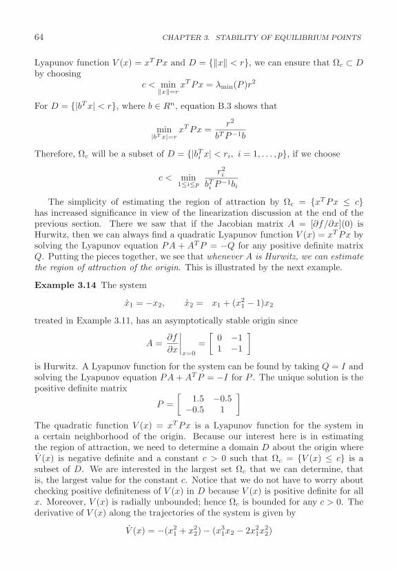
64 CHAPTER 3. STABILITY OF EQUILIBRIUM POINTS
Lyapunov function V (x) = xT Px and D = {‖x‖ < r}, we can ensure that Ωc ⊂ Dby choosing
c < min‖x‖=r
xT Px = λmin(P )r2
For D = {|bT x| < r}, where b ∈ Rn, equation B.3 shows that
min|bT x|=r
xT Px =r2
bT P−1b
Therefore, Ωc will be a subset of D = {|bTi x| < ri, i = 1, . . . , p}, if we choose
c < min1≤i≤p
r2i
bTi P−1bi
The simplicity of estimating the region of attraction by Ωc = {xT Px ≤ c}has increased significance in view of the linearization discussion at the end of theprevious section. There we saw that if the Jacobian matrix A = [∂f/∂x](0) isHurwitz, then we can always find a quadratic Lyapunov function V (x) = xT Px bysolving the Lyapunov equation PA + AT P = −Q for any positive definite matrixQ. Putting the pieces together, we see that whenever A is Hurwitz, we can estimatethe region of attraction of the origin. This is illustrated by the next example.
Example 3.14 The system
x1 = −x2, x2 = x1 + (x21 − 1)x2
treated in Example 3.11, has an asymptotically stable origin since
A =∂f
∂x
∣∣∣∣x=0
=[
0 −11 −1
]is Hurwitz. A Lyapunov function for the system can be found by taking Q = I andsolving the Lyapunov equation PA + AT P = −I for P . The unique solution is thepositive definite matrix
P =[
1.5 −0.5−0.5 1
]The quadratic function V (x) = xT Px is a Lyapunov function for the system ina certain neighborhood of the origin. Because our interest here is in estimatingthe region of attraction, we need to determine a domain D about the origin whereV (x) is negative definite and a constant c > 0 such that Ωc = {V (x) ≤ c} is asubset of D. We are interested in the largest set Ωc that we can determine, thatis, the largest value for the constant c. Notice that we do not have to worry aboutchecking positive definiteness of V (x) in D because V (x) is positive definite for allx. Moreover, V (x) is radially unbounded; hence Ωc is bounded for any c > 0. Thederivative of V (x) along the trajectories of the system is given by
V (x) = −(x21 + x2
2) − (x31x2 − 2x2
1x22)
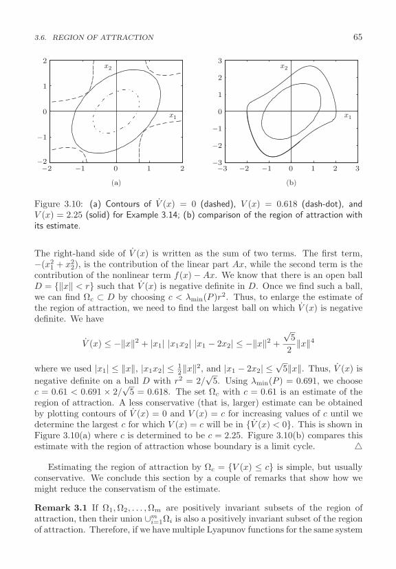
3.6. REGION OF ATTRACTION 65
−2 −1 0 1 2−2
−1
0
1
2
−3 −2 −1 0 1 2 3−3
−2
−1
0
1
2
3x2 x2
x1 x1
(a) (b)
Figure 3.10: (a) Contours of V (x) = 0 (dashed), V (x) = 0.618 (dash-dot), andV (x) = 2.25 (solid) for Example 3.14; (b) comparison of the region of attraction withits estimate.
The right-hand side of V (x) is written as the sum of two terms. The first term,−(x2
1 + x22), is the contribution of the linear part Ax, while the second term is the
contribution of the nonlinear term f(x) − Ax. We know that there is an open ballD = {‖x‖ < r} such that V (x) is negative definite in D. Once we find such a ball,we can find Ωc ⊂ D by choosing c < λmin(P )r2. Thus, to enlarge the estimate ofthe region of attraction, we need to find the largest ball on which V (x) is negativedefinite. We have
V (x) ≤ −‖x‖2 + |x1| |x1x2| |x1 − 2x2| ≤ −‖x‖2 +√
52
‖x‖4
where we used |x1| ≤ ‖x‖, |x1x2| ≤ 12‖x‖2, and |x1 − 2x2| ≤
√5‖x‖. Thus, V (x) is
negative definite on a ball D with r2 = 2/√
5. Using λmin(P ) = 0.691, we choosec = 0.61 < 0.691 × 2/
√5 = 0.618. The set Ωc with c = 0.61 is an estimate of the
region of attraction. A less conservative (that is, larger) estimate can be obtainedby plotting contours of V (x) = 0 and V (x) = c for increasing values of c until wedetermine the largest c for which V (x) = c will be in {V (x) < 0}. This is shown inFigure 3.10(a) where c is determined to be c = 2.25. Figure 3.10(b) compares thisestimate with the region of attraction whose boundary is a limit cycle. �
Estimating the region of attraction by Ωc = {V (x) ≤ c} is simple, but usuallyconservative. We conclude this section by a couple of remarks that show how wemight reduce the conservatism of the estimate.
Remark 3.1 If Ω1,Ω2, . . . ,Ωm are positively invariant subsets of the region ofattraction, then their union ∪m
i=1Ωi is also a positively invariant subset of the regionof attraction. Therefore, if we have multiple Lyapunov functions for the same system

66 CHAPTER 3. STABILITY OF EQUILIBRIUM POINTS
and each function is used to estimate the region of attraction, we can enlarge theestimate by taking the union of all the estimates. This idea will be illustrated inExample 7.14.
Remark 3.2 According to Theorem 3.5, we can work with any compact set Γ ⊂D provided we can show that Γ is positively invariant. This typically requiresinvestigating the vector field at the boundary of Γ to ensure that trajectories startingin Γ cannot leave it. The next example illustrates this idea.
Example 3.15 Consider the system23
x1 = x2, x2 = −4(x1 + x2) − h(x1 + x2)
where h is a locally Lipschitz function that satisfies
h(0) = 0; uh(u) ≥ 0, ∀ |u| ≤ 1
Consider the quadratic function
V (x) = xT
[2 11 1
]x = 2x2
1 + 2x1x2 + x22
as a Lyapunov function candidate.24 The derivative V (x) is given by
V (x) = (4x1 + 2x2)x1 + 2(x1 + x2)x2
= −2x21 − 6(x1 + x2)2 − 2(x1 + x2)h(x1 + x2)
≤ −2x21 − 6(x1 + x2)2, ∀ |x1 + x2| ≤ 1
= −xT
[8 66 6
]x
Therefore, V (x) is negative definite in the set G = {|x1 + x2| ≤ 1} and we can con-clude that the origin is asymptotically stable. To estimate the region of attraction,let us start by an estimate of the form Ωc = {V (x) ≤ c}. The largest c > 0 forwhich Ωc ⊂ G is given by
c = min|x1+x2|=1
xT Px =1
bT P−1b= 1
where bT = [1 1]. The set Ωc with c = 1 is shown in Figure 3.11. We can obtaina better estimate by not restricting ourselves to the form Ωc. A key point in thedevelopment is to observe that trajectories inside G cannot leave through certainsegments of the boundary |x1 + x2| = 1. This can be seen by examining the vector
23The example is taken from [148].24This Lyapunov function candidate can be derived by using the variable gradient method or
by applying the circle criterion of Section 7.3 and the Kalman–Yakubovich–Popov lemma.

3.6. REGION OF ATTRACTION 67
−5 0 5−5
0
5
V (x) = 10
V(x) = 1
x2
x1
(3,−4)
(−3, 4)
Figure 3.11: Estimates of the region of attraction for Example 3.15.
field at the boundary or by the following analysis: Let σ = x1 + x2 such that theboundary of G is given by σ = 1 and σ = −1. The derivative of σ2 along thetrajectories of the system is given by
d
dtσ2 = 2σ(x1 + x2) = 2σx2 − 8σ2 − 2σh(σ) ≤ 2σx2 − 8σ2, ∀ |σ| ≤ 1
On the boundary σ = 1,
d
dtσ2 ≤ 2x2 − 8 ≤ 0, ∀ x2 ≤ 4
This implies that when the trajectory is at any point on the segment of the boundaryσ = 1 for which x2 ≤ 4, it cannot move outside the set G because at such point σ2
is nonincreasing. Similarly, on the boundary σ = −1,
d
dtσ2 ≤ −2x2 − 8 ≤ 0, ∀ x2 ≥ −4
Hence, the trajectory cannot leave the set G through the segment of the boundaryσ = −1 for which x2 ≥ −4. This information can be used to form a closed, bounded,positively invariant set Γ that satisfies the conditions of Theorem 3.5. Using thetwo segments of the boundary of G just identified to define the boundary of Γ, wenow need two other segments to close the set. These segments should have theproperty that trajectories cannot leave the set through them. We can take themas segments of a Lyapunov surface. Let c1 be such that the Lyapunov surfaceV (x) = c1 intersects the boundary x1 + x2 = 1 at x2 = 4, that is, at the point(−3, 4). (See Figure 3.11.) Let c2 be such that the Lyapunov surface V (x) = c2
intersects the boundary x1 +x2 = −1 at x2 = −4, that is, at the point (3,−4). Therequired Lyapunov surface is defined by V (x) = min{c1, c2}. The constants c1 and

68 CHAPTER 3. STABILITY OF EQUILIBRIUM POINTS
c2 are given by
c1 = V (x)|x1=−3,x2=4 = 10, c2 = V (x)|x1=3,x2=−4 = 10
Therefore, we take c = 10 and define the set Γ by
Γ = {V (x) ≤ 10 and |x1 + x2| ≤ 1}
This set is closed, bounded, and positively invariant. Moreover, V (x) is negativedefinite in Γ, since Γ ⊂ G. Thus, we conclude by Theorem 3.5 that Γ is a subset ofthe region of attraction. �
3.7 Converse Lyapunov Theorems
Theorems 3.3 and 3.6 establish asymptotic stability or exponential stability of theorigin by requiring the existence of a Lyapunov function V (x) that satisfies certainconditions. Requiring the existence of an auxiliary function V (x) that satisfies cer-tain conditions is typical in many theorems of Lyapunov’s method. The conditionsof these theorems cannot be checked directly on the data of the problem. Instead,one has to search for the auxiliary function. Faced with this searching problem,two questions come to mind. First, is there a function that satisfies the conditionsof the theorem? Second, how can we search for such a function? In many cases,Lyapunov theory provides an affirmative answer to the first question. The answertakes the form of a converse Lyapunov theorem, which is the inverse of one of Lya-punov’s theorems. For example, a converse theorem for asymptotic stability wouldconfirm that if the origin is asymptotically stable, then there is a Lyapunov functionthat satisfies the conditions of Theorem 3.3. Most of these converse theorems areproven by actually constructing auxiliary functions that satisfy the conditions ofthe respective theorems. Unfortunately, this construction almost always assumesknowledge of the solution of the differential equation. Therefore, the theorems donot help in the practical search for an auxiliary function. However, they are use-ful in using Lyapunov theory to draw conceptual conclusions about the behaviorof dynamical systems, as in Example 3.16. In this section, we give two converseLyapunov theorems without proofs.25 The first one is for the case when the originis exponentially stable, and the second when it is asymptotically stable.
Theorem 3.8 Let x = 0 be an exponentially stable equilibrium point for the n-dimensional system x = f(x), where f is continuously differentiable on D = {‖x‖ <r}. Let k, λ, and r0 be positive constants with r0 < r/k such that
‖x(t)‖ ≤ k‖x(0)‖e−λt, ∀ x(0) ∈ D0, ∀ t ≥ 0
25The proofs are given in [74]; see Theorems 4.14 and 4.17, respectively.
3.7. CONVERSE LYAPUNOV THEOREMS 69
where D0 = {‖x‖ < r0}. Then, there is a continuously differentiable function V (x)that satisfies the inequalities
c1‖x‖2 ≤ V (x) ≤ c2‖x‖2,∂V
∂xf(x) ≤ −c3‖x‖2,
∥∥∥∥∂V
∂x
∥∥∥∥ ≤ c4‖x‖
for all x ∈ D0, with positive constants c1, c2, c3, and c4. Moreover, if f is continu-ously differentiable for all x, globally Lipschitz, and the origin is globally exponen-tially stable, then V (x) is defined and satisfies the aforementioned inequalities forall x ∈ Rn. �
Theorem 3.9 Let x = 0 be an asymptotically stable equilibrium point for the n-dimensional system x = f(x), where f is locally Lipschitz on a domain D ⊂ Rn
that contains the origin. Let RA ⊂ D be the region of attraction of x = 0. Then,there is a smooth, positive definite function V (x) and a continuous, positive definitefunction W (x), both defined for all x ∈ RA, such that
V (x) → ∞ as x → ∂RA
∂V
∂xf(x) ≤ −W (x), ∀ x ∈ RA
and for any c > 0, {V (x) ≤ c} is a compact subset of RA. When RA = Rn, V (x)is radially unbounded. �
As an example of the use of converse Lyapunov functions, we show how Theo-rem 3.8 can be used to prove the necessity part of the first item of Theorem 3.2.
Example 3.16 Consider the system x = f(x) where f is continuously differentiablein the neighborhood of the origin and f(0) = 0. Show that the origin is exponentiallystable only if A = [∂f/∂x](0) is Hurwitz. To proceed, let us recall that
f(x) = Ax + G(x)x
where G(x) → 0 as x → 0. Hence, given any L > 0, there is r1 > 0 such that‖G(x)‖ ≤ L for all ‖x‖ < r1. Rewrite the linear system x = Ax as
x = Ax = f(x) − G(x)x
Because the origin of x = f(x) is exponentially stable, let V (x) be the functionprovided by Theorem 3.8 over the domain {‖x‖ < r0}. Using V (x) as a Lyapunovfunction candidate for x = Ax, we obtain
∂V
∂xAx =
∂V
∂xf(x) − ∂V
∂xG(x)x ≤ −c3‖x‖2 + c4L‖x‖2 < (c3 − c4L)‖x‖2
Taking L < c3/c4), we see that the foregoing inequality holds for all ‖x‖ < min{r0, r1}.Hence, by Theorem 3.6, the origin of x = Ax is exponentially stable.

70 CHAPTER 3. STABILITY OF EQUILIBRIUM POINTS
3.8 Exercises
3.1 Show that the scalar system x = (k−x2)/x, with k > 0, has two asymptoticallystable equilibrium points and find their regions of attraction.
3.2 Consider the scalar system x = −g(x), where g(x) is locally Lipschitz and
g(0) = 0; xg(x) > 0, ∀ x = 0 and x ∈ (−a, a)
It is shown in Section 3.1 that the origin is asymptotically stable. In this exercisewe arrive at the same conclusion using Lyapunov functions.
(a) Show that the asymptotic stability conditions of Theorem 3.3 are satisfied withV (x) = 1
2x2 or V (x) =∫ x
0g(y) dy.
(b) If xg(x) > 0 for all x = 0, show that the global asymptotic stability conditionsof Theorem 3.3 are satisfied with V (x) = 1
2x2 or V (x) = 12x2 +
∫ x
0g(y) dy.
(c) Under what conditions on g can you show global asymptotic stability usingV (x) =
∫ x
0g(y) dy? Give an example of g where the origin of x = −g(x)
is globally asymptotic stability but V (x) =∫ x
0g(y) dy does not satisfy the
global asymptotic stability conditions of Theorem 3.3.
3.3 For each of the following scalar systems, determine if the origin is unstable,stable but not asymptotically stable, asymptotically stable but not globally asymp-totically stable, or globally asymptotically stable.
(1) f(x) = −x for x ≥ 0 and f(x) = 0 for x < 0
(2) f(x) = x for x ≥ 0 and f(x) = 0 for x < 0
(3) f(x) = sinx
(4) f(x) = − sin x
(5) f(x) = −x − sin x
3.4 Euler equations for a rotating rigid spacecraft are given by [105]
J1ω1 = (J2−J3)ω2ω3+u1, J2ω2 = (J3−J1)ω3ω1+u2, J3ω3 = (J1−J2)ω1ω2+u3
where ω = col(ω1, ω2, ω3) is the angular velocity vector along the principal axes,u = col(u1, u2, u3) is the vector of torque inputs applied about the principal axes,and J1 to J3 are the principal moments of inertia.
(a) Show that with u = 0 the origin ω = 0 is stable. Is it asymptotically stable?
(b) Let ui = −kiωi, where k1 to k3 are positive constants. Show that the origin ofthe closed-loop system is globally asymptotically stable.
3.8. EXERCISES 71
3.5 For each of the following systems, determine whether the origin is stable,asymptotically stable or unstable.
(1) x1 = x2, x2 = x3, x3 = −2 sin x1 − 2x2 − 2x3
(2) x1 = x2, x2 = x3, x3 = 2 sin x1 − 2x2 − 2x3
(3) x1 = x2 + x3, x2 = − sin x1 − x3, x3 = − sin x1 + x2
3.6 Consider the system
x1 = x2, x2 = −h(x1) − 2x2, where h(x1) = x1
(2 +
x21
1 + x21
)
Verify that V (x) =∫ x1
0h(σ) dσ + 1
2 (x1 + x2)2 is positive definite and radiallyunbounded; then use it to show that the origin is globally exponentially stable.
3.7 Consider the system
x1 = −x1 + x3, x2 = x3, x3 = −x2 − x32 − x3
(a) Is the origin exponentially stable?
(b) Using V (x) = bx21 + 3x2
2 + 2x2x3 + 2x23 + x4
2, where b > 0 is to be chosen, showthat the origin is globally asymptotically stable.
3.8 ([132]) Consider the system
x1 = x2, x2 = − tanh(x1 + x2)
(a) Show that
V (x) =∫ x1
0
tanh(σ) dσ +∫ x1+x2
0
tanh(σ) dσ + x22
is positive definite for all x and radially unbounded.
(b) Show that the origin is globally asymptotically stable.
3.9 (Krasovskii’s Method) Consider the system x = f(x) with f(0) = 0. As-sume that f(x) is continuously differentiable and its Jacobian [∂f/∂x] satisfies
P
[∂f
∂x(x)]
+[∂f
∂x(x)]T
P ≤ −I, ∀ x ∈ Rn, where P = PT > 0
(a) Using the representation f(x) =∫ 1
0∂f∂x (σx)x dσ, show that
xT Pf(x) + fT (x)Px ≤ −xT x, ∀ x ∈ Rn

72 CHAPTER 3. STABILITY OF EQUILIBRIUM POINTS
(b) Using V (x) = fT (x)Pf(x), show that the origin is globally asymptoticallystable.
3.10 ([121]) A closed-loop system under optimal stabilizing control is given by
x = f(x) − kG(x)R−1(x)GT (x)(
∂V
∂x
)T
where V (x) is a continuously differentiable, positive definite function that satisfiesthe Hamilton–Jacobi–Bellman equation
∂V
∂xf(x) + q(x) − 1
4
∂V
∂xG(x)R−1(x)GT (x)
(∂V
∂x
)T
= 0
q(x) is a positive semidefinite function, R(x) is a positive definite matrix for all x,and k is a positive constant. Show that the origin is asymptotically stable when
(1) q(x) is positive definite and k ≥ 1/4.
(2) q(x) is positive semidefinite, k > 1/4, and the only solution of x = f(x) thatstays identically in the set {q(x) = 0} is the trivial solution x(t) ≡ 0.
3.11 The system
x1 = −x1 + x3, x2 = x3, x3 = −g1(x1) − g2(x2) − x3
where g1 and g2 are locally Lipschitz and satisfy gi(0) = 0 and ygi(y) > 0 for ally = 0, has a unique equilibrium point at the origin.
(a) Verify that V (x) =∫ x1
0g1(y) dy +
∫ x2
0g2(y) dy + 1
2x23 is positive definite for all
x and use it to show asymptotic stability of the origin.
(b) Under what additional conditions on g1 and g2 can you show that the origin isglobally asymptotically stable.
(c) Under what additional conditions on g1 and g2 can you show that the origin isexponentially stable?
3.12 An unforced mass-spring system (Section A.2) with nonlinear viscous frictionand nonlinear spring is modeled by
my + b(1 + c|y|)y + g(y) = 0
where g(y) = k(1−a2y2)y, with |ay| < 1, for a softening spring, g(y) = k(1+a2y2)yfor a hardening spring, and all constants are positive. Take the state variables asx1 = y, x2 = y. Using an energy-type Lyapunov function, study the stability of theorigin for each spring type.
3.8. EXERCISES 73
3.13 Show that the origin of the system
x1 = x2, x2 = −x1 + μx2 − x32
is globally asymptotically stable for μ ≤ 0 and unstable for μ > 0. Is it exponentiallystable when μ = 0 ?
3.14 Using V (x) = 12xT x, show that the origin of
x1 = −x1 + x2 cos x1, x2 = x1 cos x1 − x2(cos x1)2 + x3, x3 = −x2
is globally asymptotically stable. Is it exponentially stable?
3.15 Consider the pendulum equation
x1 = x2, x2 = − sin x1 − bx2 + u
under the state feedback control u = −k1 sat(x1) − k2 sat(x2), where b, k1 and k2
are positive constants and k1 > 1.
(a) Show that the origin is the unique equilibrium point of the closed-loop system.
(b) Using V (x) =∫ x1
0[sin σ + k1 sat(σ)] dσ + 1
2x22, show that the origin of the
closed-loop system is globally asymptotically stable.
3.16 For each of the following systems,
(a) Find all equilibrium points and study their stability using linearization.
(b) Using quadratic Lyapunov functions, estimate the regions of the attraction ofeach asymptotically stable equilibrium point. Try to make the estimates aslarge as you can.
(c) Draw the phase portrait of the system to find the exact regions of attractionand compare them with your estimates.
(1) x1 = −(x1 + x31) + 2x2, x2 = 2x1 − (x2 + x3
2)
(2) x1 = x1 − x31 + x2, x2 = x1 − 3x2
(3) x1 = x2, x2 = −x1 − x2 + 2x32 − 1
2x52
(4) x1 = −x2, x2 = 2x1 + 3x2 + 2 sat(−3x2)
3.17 Consider the system
x1 = x2, x2 = −x1 + x51 − x2
(a) Using the Lyapunov function candidate V (x) = 12x2
1 − 16x6
1 + 12x2
2, show thatthe origin is asymptotically stable and estimate the region of attraction.
74 CHAPTER 3. STABILITY OF EQUILIBRIUM POINTS
(b) Draw the phase portrait of the system to find the exact region of attractionand compare it with your estimate.
3.18 Consider the system
x1 = x31 − x2, x2 = x1 − x2
Show that the origin is asymptotically stable? Is it exponentially stable? Is itglobally asymptotically stable? If not, estimate the region of attraction.
3.19 For each of the following systems, show that there is an equilibrium pointat the origin and investigate its stability. If the origin is asymptotically stable,determine if it is globally asymptotically stable; if it is not so, estimate the regionof attraction.
(1) x1 = x2, x2 = −x31 − x2
(2) x1 = x2, x2 = −x31
(3) x1 = x2, x2 = −x1 − 2x2 − (x21 + x2
2) tanh(x1 + x2)
(4) x1 = x2, x2 = −x1 + 13x3
1 − 2x2
(5) x1 = −x31 + x2, x2 = −x3
1 − x2
3.20 Show that the origin of the system
x1 = −x1 + x2, x2 = −0.1x31 − x2 − 10 sin x3, x3 = x2 − x3
is asymptotically stable and estimate the region of attraction.
3.21 ([148]) Consider the system
x1 = x2, x2 = −x1 − x2 − (x1 + 2x2)(1 − x22)
Show that the origin is asymptotically stable and find an estimate of the regionof attraction that includes the point x = (−1, 1). Hint: Use the variable gradientmethod to find a quadratic Lyapunov function V (x) = xT Px such that V (x) isnegative definite in the set {|x2| ≤ 1}.
Chapter 4
Time-Varying and PerturbedSystems
The chapter starts in Section 4.1 by extending Lyapunov stability theory to time-varying systems. Towards that end, we introduce class K and class KL functions,which will be used extensively in the rest of the chapter, and indeed the rest of thebook. We use them to define uniform stability and uniform asymptotic stability ofequilibrium points of time-varying systems, and give Lyapunov theorems for theseproperties. The chapter turns then to the study of perturbed systems of the form
x = f(x) + g(t, x)
when the origin of x = f(x) is asymptotically stable. Two cases are studied sepa-rately. Vanishing perturbations, when g(t, 0) = 0, are studied in Section 4.2 wherethe goal is to find conditions on g under which we can confirm that the origin ofthe perturbed system is uniformly asymptotically, or exponentially, stable. Nonva-nishing perturbations, when g(t, 0) = 0, are studied in Section 4.3 after introducingthe notion of ultimate boundedness and giving Lyapunov-like theorems for it.1 Theresults on ultimate boundedness lead naturally to the notion of input-to-state sta-bility, which is introduced in Section 4.4 together with its Lyapunov-like theorems.
4.1 Time-Varying Systems
Consider the n-dimensional time-varying system
x = f(t, x) (4.1)
1The nonvanishing perturbation is referred to in [54, 78] as “persistent disturbance.” Theresults on nonvanishing perturbations are related to the concept of total stability [54, Section 56].
75

76 CHAPTER 4. TIME-VARYING AND PERTURBED SYSTEMS
where f(t, x) is piecewise continuous in t and locally Lipschitz in x for all t ≥ 0and x ∈ D, where D ⊂ Rn is a domain that contains the origin x = 0. The originis an equilibrium point of (4.1) at t = 0 if f(t, 0) = 0, ∀ t ≥ 0. The notions ofstability and asymptotic stability of equilibrium points of time-varying systems arebasically the same as those introduced in Definition 3.1 for time-invariant systems.The new element here is that, while the solution of a time-invariant system dependsonly on (t − t0), the solution of a time-varying system may depend on both t andt0. Therefore, the stability behavior of the equilibrium point will, in general, bedependent on t0. The origin x = 0 is a stable equilibrium point for x = f(t, x) if,for each ε > 0, and any t0 ≥ 0 there is δ > 0, dependent on both ε and t0, such that
‖x(t0)‖ < δ ⇒ ‖x(t)‖ < ε, ∀ t ≥ t0
The existence of δ for every t0 does not necessarily guarantee that there is one δ,dependent only on ε, that works for all t0. Similar dependence on t0 appears instudying asymptotic stability. Therefore, we refine Definition 3.1 to define stabilityand asymptotic stability as uniform properties with respect to the initial time. Thenew definition will use class K and class KL functions, which are defined next.
Definition 4.1
• A scalar continuous function α(r), defined for r ∈ [0, a), belongs to class K ifit is strictly increasing and α(0) = 0. It belongs to class K∞ if it is definedfor all r ≥ 0 and α(r) → ∞ as r → ∞.
• A scalar continuous function β(r, s), defined for r ∈ [0, a) and s ∈ [0,∞),belongs to class KL if, for each fixed s, the mapping β(r, s) belongs to class Kwith respect to r and, for each fixed r, the mapping β(r, s) is decreasing withrespect to s and β(r, s) → 0 as s → ∞.
Example 4.1
• α(r) = tan−1(r) is strictly increasing since α′(r) = 1/(1 + r2) > 0. It belongsto class K, but not to class K∞ since limr→∞ α(r) = π/2 < ∞.
• α(r) = rc, with c > 0, is strictly increasing since α′(r) = c rc−1 > 0. More-over, limr→∞ α(r) = ∞; thus, it belongs to class K∞.
• α(r) = min{r, r2} is continuous, strictly increasing, and limr→∞ α(r) = ∞.Hence, it belongs to class K∞. It is not continuously differentiable at r = 1.Continuous differentiability is not required for a class K function.
• β(r, s) = r/(ksr +1), with positive constant k, belongs to class KL because itis strictly increasing in r since ∂β/∂r = 1/(ksr + 1)2 > 0, strictly decreasingin s since ∂β/∂s = −kr2/(ksr + 1)2 < 0, and β(r, s) → 0 as s → ∞.
• β(r, s) = rce−as, with positive constants a and c, belongs to class KL.
4.1. TIME-VARYING SYSTEMS 77
The next two lemmas state some properties of class K and class KL functions.2
Lemma 4.1 Let α1 and α2 be class K functions on [0, a1) and [0, a2), respectively,with a1 ≥ limr→a2 α2(r), and β be a class KL function defined on [0, limr→a2 α2(r))×[0,∞) with a1 ≥ limr→a2 β(α2(r), 0). Let α3 and α4 be class K∞ functions. Denotethe inverse of αi by α−1
i . Then,
• α−11 is defined on [0, limr→a1 α1(r)) and belongs to class K.
• α−13 is defined on [0,∞) and belongs to class K∞.
• α1 ◦ α2 is defined on [0, a2) and belongs to class K.
• α3 ◦ α4 is defined on [0,∞) and belongs to class K∞.
• σ(r, s) = α1(β(α2(r), s)) is defined on [0, a2)× [0,∞) and belongs to class KL.�
Lemma 4.2 Let V : D → R be a continuous positive definite function defined on adomain D ⊂ Rn that contains the origin. Let Br ⊂ D for some r > 0. Then, thereexist class K functions α1 and α2, defined on [0, r], such that
α1(‖x‖) ≤ V (x) ≤ α2(‖x‖)
for all x ∈ Br. If D = Rn and V (x) is radially unbounded, then there exist classK∞ functions α1 and α2 such the foregoing inequality holds for all x ∈ Rn. �
Definition 4.2 The equilibrium point x = 0 of x = f(t, x) is
• uniformly stable if there exist a class K function α and a positive constant c,independent of t0, such that
‖x(t)‖ ≤ α(‖x(t0)‖), ∀ t ≥ t0 ≥ 0, ∀ ‖x(t0)‖ < c
• uniformly asymptotically stable if there exist a class KL function β and apositive constant c, independent of t0, such that
‖x(t)‖ ≤ β(‖x(t0)‖, t − t0), ∀ t ≥ t0 ≥ 0, ∀ ‖x(t0)‖ < c
• globally uniformly asymptotically stable if the foregoing inequality holds ∀ x(t0).
• exponentially stable if there exist positive constants c, k, and λ such that
‖x(t)‖ ≤ k‖x(t0)‖e−λ(t−t0), ∀ ‖x(t0)‖ < c
• globally exponentially stable if the foregoing inequality holds ∀ x(t0). �
2The proof of Lemma 4.1 is straightforward and that of 4.2 is given in [74, Lemma 4.3].
78 CHAPTER 4. TIME-VARYING AND PERTURBED SYSTEMS
The following three theorems, stated without proofs,3 extend Theorems 3.3 and3.6 to time-varying systems.
Theorem 4.1 Let the origin x = 0 be an equilibrium point of x = f(t, x) andD ⊂ Rn be a domain containing x = 0. Suppose f(t, x) is piecewise continuous int and locally Lipschitz in x for all t ≥ 0 and x ∈ D. Let V (t, x) be a continuouslydifferentiable function such that
W1(x) ≤ V (t, x) ≤ W2(x) (4.2)
∂V
∂t+
∂V
∂xf(t, x) ≤ 0 (4.3)
for all t ≥ 0 and x ∈ D, where W1(x) and W2(x) are continuous positive definitefunctions on D. Then, the origin is uniformly stable. �
Theorem 4.2 Suppose the assumptions of Theorem 4.1 are satisfied with inequality(4.3) strengthened to
∂V
∂t+
∂V
∂xf(t, x) ≤ −W3(x) (4.4)
for all t ≥ 0 and x ∈ D, where W3(x) is a continuous positive definite functionon D. Then, the origin is uniformly asymptotically stable. Moreover, if r and care chosen such that Br = {‖x‖ ≤ r} ⊂ D and c < min‖x‖=r W1(x), then everytrajectory starting in {x ∈ Br | W2(x) ≤ c} satisfies
‖x(t)‖ ≤ β(‖x(t0)‖, t − t0), ∀ t ≥ t0 ≥ 0
for some class KL function β. Finally, if D = Rn and W1(x) is radially unbounded,then the origin is globally uniformly asymptotically stable. �
Theorem 4.3 Suppose the assumptions of Theorem 4.1 are satisfied with inequal-ities (4.2) and (4.3) strengthened to
k1‖x‖a ≤ V (t, x) ≤ k2‖x‖a (4.5)
∂V
∂t+
∂V
∂xf(t, x) ≤ −k3‖x‖a (4.6)
for all t ≥ 0 and x ∈ D, where k1, k2, k3, and a are positive constants. Then, theorigin is exponentially stable. If the assumptions hold globally, the origin will beglobally exponentially stable. �
A function V (t, x) is said to be positive semidefinite if V (t, x) ≥ 0. It is saidto be positive definite if V (t, x) ≥ W1(x) for some positive definite function W1(x),radially unbounded if W1(x) is so, and decrescent if V (t, x) ≤ W2(x). A functionV (t, x) is said to be negative definite (semidefinite) if −V (t, x) is positive definite
3The proofs can be found in [74, Section 4.5].
4.1. TIME-VARYING SYSTEMS 79
(semidefinite). Therefore, Theorems 4.1 and 4.2 say that the origin is uniformlystable if there is a continuously differentiable, positive definite, decrescent functionV (t, x), whose derivative along the trajectories of the system is negative semidefinite.It is uniformly asymptotically stable if the derivative is negative definite, and globallyuniformly asymptotically stable if the conditions for uniform asymptotic stabilityhold globally with a radially unbounded V (t, x).
Example 4.2 Consider the scalar system
x = −[1 + g(t)]x3
where g(t) is continuous and g(t) ≥ 0 for all t ≥ 0. Using V (x) = 12x2, we obtain
V (t, x) = −[1 + g(t)]x4 ≤ −x4, ∀ x ∈ R, ∀ t ≥ 0
The assumptions of Theorem 4.2 are satisfied globally with W1(x) = W2(x) = V (x)and W3(x) = x4. Hence, the origin is globally uniformly asymptotically stable. Example 4.3 Consider the system
x1 = −x1 − g(t)x2, x2 = x1 − x2
where g(t) is continuously differentiable and satisfies
0 ≤ g(t) ≤ k and g(t) ≤ g(t), ∀ t ≥ 0
Taking V (t, x) = x21 + [1 + g(t)]x2
2, it can be seen that
x21 + x2
2 ≤ V (t, x) ≤ x21 + (1 + k)x2
2, ∀ x ∈ R2
Hence, V (t, x) is positive definite, decrescent, and radially unbounded. The deriva-tive of V along the trajectories of the system is given by
V (t, x) = −2x21 + 2x1x2 − [2 + 2g(t) − g(t)]x2
2
Using the inequality
2 + 2g(t) − g(t) ≥ 2 + 2g(t) − g(t) ≥ 2
we obtain
V (t, x) ≤ −2x21 + 2x1x2 − 2x2
2 = −[
x1
x2
]T [ 2 −1−1 2
] [x1
x2
]def= −xT Qx
where Q is positive definite; therefore, V (t, x) is negative definite. Thus, all theassumptions of Theorem 4.2 are satisfied globally with positive definite quadraticfunctions W1, W2, and W3. Recalling that a positive definite xT Px satisfies
λmin(P )‖x‖2 ≤ xT Px ≤ λmax(P )‖x‖2
we see that the conditions of Theorem 4.3 are satisfied globally with a = 2. Hence,the origin is globally exponentially stable.
80 CHAPTER 4. TIME-VARYING AND PERTURBED SYSTEMS
4.2 Perturbed Systems
Consider the systemx = f(x) + g(t, x) (4.7)
where f is locally Lipschitz and g is piecewise continuous in t and locally Lipschitzin x, for all t ≥ 0 and x ∈ D, in which D ⊂ Rn is a domain that contains the originx = 0. Suppose f(0) = 0 and g(t, 0) = 0 so that the origin is an equilibrium pointof the system (4.7). We think of the system (4.7) as a perturbation of the nominalsystem4
x = f(x) (4.8)
The perturbation term g(t, x) could result from modeling errors, aging, or uncertain-ties and disturbances, which exist in any realistic problem. In a typical situation,we do not know g(t, x), but we know some information about it, like knowing anupper bound on ‖g(t, x)‖. Suppose the nominal system (4.8) has an asymptoticallystable equilibrium point at the origin, what can we say about the stability of theorigin as an equilibrium point of the perturbed system (4.7)? A natural approachto address this question is to use a Lyapunov function for the nominal system as aLyapunov function candidate for the perturbed system.
Let us start with the case when the origin is an exponentially stable equilibriumpoint of the nominal system (4.8). Let V (x) be a Lyapunov function that satisfies
c1‖x‖2 ≤ V (x) ≤ c2‖x‖2,∂V
∂xf(x) ≤ −c3‖x‖2,
∥∥∥∥∂V
∂x
∥∥∥∥ ≤ c4‖x‖ (4.9)
for all x ∈ D for some positive constants c1, c2, c3, and c4.5 Suppose the perturba-tion term g(t, x) satisfies the linear growth bound
‖g(t, x)‖ ≤ γ‖x‖, ∀ t ≥ 0, ∀ x ∈ D (4.10)
where γ is a nonnegative constant. Any function g(t, x) that vanishes at the originand is locally Lipschitz in x, uniformly in t for all t ≥ 0, in a bounded neighborhoodof the origin satisfies (4.10) over that neighborhood.6 We use V as a Lyapunovfunction candidate to investigate the stability of the origin as an equilibrium pointfor the perturbed system (4.7). The derivative of V along the trajectories of (4.7)is given by
V (t, x) =∂V
∂xf(x) +
∂V
∂xg(t, x)
4For convenience, the nominal system is assumed to be time invariant. The results of thissection extend in a straightforward way to the case when the nominal system is time varying; see[74, Section 9.1].
5The existence of a Lyapunov function satisfying (4.9) is guaranteed by (the converse Lyapunov)Theorem 3.8 when f is continuously differentiable.
6Note, however, that the linear growth bound (4.10) becomes restrictive when required to holdglobally because it would require g to be globally Lipschitz in x.
4.2. PERTURBED SYSTEMS 81
The first term on the right-hand side is the derivative of V (x) along the trajectoriesof the nominal system, which is negative definite. The second term, [∂V/∂x]g, isthe effect of the perturbation. Since we do not have complete knowledge of g thebest we can do is worst case analysis where [∂V/∂x]g is bounded by a nonnegativeterm. Using (4.9) and (4.10), we obtain
V (t, x) ≤ −c3‖x‖2 +∥∥∥∥∂V
∂x
∥∥∥∥ ‖g(t, x)‖ ≤ −c3‖x‖2 + c4γ‖x‖2
If γ is small enough to satisfy the bound
γ <c3
c4(4.11)
thenV (t, x) ≤ −(c3 − γc4)‖x‖2, (c3 − γc4) > 0
In this case, we can conclude by Theorem 4.3 that the origin is an exponentiallystable equilibrium point of the perturbed system (4.7).
Example 4.4 Consider the system
x = Ax + g(t, x)
where A is Hurwitz and ‖g(t, x)‖ ≤ γ‖x‖ for all t ≥ 0 and x ∈ Rn. Let Q = QT > 0and solve the Lyapunov equation PA + AT P = −Q for P . From Theorem 3.7,we know that there is a unique solution P = PT > 0. The quadratic Lyapunovfunction V (x) = xT Px satisfies (4.9). In particular,
λmin(P )‖x‖2 ≤ V (x) ≤ λmax(P )‖x‖2
∂V
∂xAx = −xT Qx ≤ −λmin(Q)‖x‖2
∥∥∥∥∂V
∂x
∥∥∥∥ = ‖2xT P‖ ≤ 2‖P‖‖x‖ = 2λmax(P )‖x‖
The derivative of V (x) along the trajectories of the perturbed system satisfies
V (t, x) ≤ −λmin(Q)‖x‖2 + 2λmax(P )γ‖x‖2
Hence, the origin is globally exponentially stable if γ < λmin(Q)/(2λmax(P )). Sincethis bound depends on the choice of Q, one may wonder how to choose Q to maxi-mize the ratio λmin(Q)/λmax(P ). It turns out that this ratio is maximized with thechoice Q = I.7
7See [74, Exercise 9.1].
82 CHAPTER 4. TIME-VARYING AND PERTURBED SYSTEMS
Example 4.5 Consider the two-dimensional system
x1 = x2, x2 = −4x1 − 2x2 + βx32
where the constant β ≥ 0 is unknown. We view the system as a perturbed systemof the form (4.7) with
f(x) = Ax =[
0 1−4 −2
] [x1
x2
]and g(x) =
[0
βx32
]
The eigenvalues of A are −1 ± j√
3. Hence, A is Hurwitz. The solution of theLyapunov equation PA + AT P = −I is
P =
⎡⎣ 3
218
18
516
⎤⎦
As we saw in Example 4.4, the Lyapunov function V (x) = xT Px satisfies (4.9)with c3 = 1 and c4 = 2λmax(P ) = 2 × 1.513 = 3.026. The perturbation term g(x)does not satisfy the linear growth condition ‖g(x)‖ ≤ γ‖x‖ globally, but satisfies itover compact sets. Consider the compact set Ωc = {xT Px ≤ c} for c > 0 and letk2 = maxx∈Ωc
|x2|. Then, by (B.4),
k2 = maxxT Px≤c
| [ 0 1]x| =
√c‖ [ 0 1
]P−1/2‖ = 1.8194
√c
where P−1/2 is the inverse of P 1/2, the square root matrix of P . Using V (x) as aLyapunov function candidate for the perturbed system, we obtain
V (x) ≤ −‖x‖2 + 3.026βk22‖x‖2
Hence, V (x) will be negative definite in Ωc if
β <1
3.026k22
=1
3.026 × (1.8194)2c≈ 0.1
c
We conclude that if β < 0.1/c, the origin will be exponentially stable and Ωc willbe an estimate of the region of attraction. Let us use this example to illustrate theconservative nature of the bound (4.11). Using this bound, we came up with theinequality β < 1/(3.026k2
2), which allows the perturbation term g(t, x) to be anytwo-dimensional vector that satisfies ‖g(t, x)‖ ≤ βk2
2‖x‖. This class of perturbationsis more general than the perturbation we have in this specific problem. We havea structured perturbation in the sense that the first component of g is always zero,while our analysis allowed for unstructured perturbation where the vector g couldchange in all directions. Such disregard of the structure of the perturbation will,in general, lead to conservative bounds. Suppose we repeat the analysis, this timetaking into consideration the structure of the perturbation. Instead of using the
4.2. PERTURBED SYSTEMS 83
general bound of (4.11), we calculate the derivative of V (x) along the trajectoriesof the perturbed system to obtain
V (x) = −‖x‖2 + 2xT Pg(x) = −‖x‖2 + 18βx3
2(2x1 + 5x2)
≤ −‖x‖2 +√
298 βk2
2‖x‖2
where we wrote (2x1 +5x2) as yT x and used the inequality |yT x| ≤ ‖x‖‖y‖. Hence,V (x) is negative definite for β < 8/(
√29k2
2). Using, again, the fact that for allx ∈ Ωc, |x2|2 ≤ k2
2 = (1.8194)2c, we arrive at the bound β < 0.448/c, which ismore than four times the bound we obtained by using (4.11). Finally, note thatthe inequality β < 0.448/c shows a tradeoff between the estimate of the regionof attraction and the estimate of the upper bound on β. The smaller the upperbound on β, the larger the estimate of the region of attraction. This tradeoff is notartificial; it does exist in this example. The change of variables
z1 =
√3β
2x2, z2 =
√3β
8(4x1 + 2x2 − βx3
2), τ = 2t
transforms the state equation into
dz1
dτ= −z2,
dz2
dτ= z1 + (z2
1 − 1)z2
which was shown in Example 3.11 to have a bounded region of attraction surroundedby an unstable limit cycle. When transformed into the x-coordinates, the region ofattraction will expand with decreasing β and shrink with increasing β.
When the origin of the nominal system x = f(x) is asymptotically, but notexponentially, stable, the stability analysis of the perturbed system is more involved.Suppose the nominal system has a positive definite Lyapunov function V (x) thatsatisfies
∂V
∂xf(x) ≤ −W3(x)
for all x ∈ D, where W3(x) is positive definite and continuous. The derivative of Valong the trajectories of (4.7) is given by
V (t, x) =∂V
∂xf(x) +
∂V
∂xg(t, x) ≤ −W3(x) +
∥∥∥∥∂V
∂xg(t, x)
∥∥∥∥Our task now is to show that ‖[∂V/∂x]g(t, x)‖ < W3(x) for all t ≥ 0 and x ∈ D,a task that cannot be done by putting a linear growth bound on ‖g(t, x)‖, as wehave done in the exponential stability case. The growth bound on ‖g(t, x)‖ willdepend on the nature of the Lyapunov function of the nominal system. One classof Lyapunov functions for which the analysis is almost as simple as in exponentialstability is the case when V (x) satisfies
∂V
∂xf(x) ≤ −c3φ
2(x),∥∥∥∥∂V
∂x
∥∥∥∥ ≤ c4φ(x) (4.12)
84 CHAPTER 4. TIME-VARYING AND PERTURBED SYSTEMS
for all x ∈ D for some positive constants c3 and c4, where the scalar functionφ(x) is positive definite and continuous. A function satisfying (4.12) is called aquadratic-type Lyapunov function. It is clear that a Lyapunov function satisfying(4.9) is quadratic type, but a quadratic-type Lyapunov function may exist evenwhen the origin is not exponentially stable. We will illustrate this point shortlyby an example. If the nominal system x = f(x) has a quadratic-type Lyapunovfunction V (x), then its derivative along the trajectories of (4.7) satisfies
V (t, x) ≤ −c3φ2(x) + c4φ(x)‖g(t, x)‖
Suppose now that the perturbation term satisfies the bound
‖g(t, x)‖ ≤ γφ(x), with γ <c3
c4
Then,V (t, x) ≤ −(c3 − c4γ)φ2(x)
which shows that V (t, x) is negative definite.
Example 4.6 Consider the scalar system
x = −x3 + g(t, x)
The nominal system x = −x3 has a globally asymptotically stable equilibriumpoint at the origin, but, as we saw in Example 3.2, the origin is not exponentiallystable. Thus, there is no Lyapunov function that satisfies (4.9). The Lyapunovfunction V (x) = x4 satisfies (4.12), with φ(x) = |x|3 and c3 = c4 = 4. Suppose theperturbation term g(t, x) satisfies the bound |g(t, x)| ≤ γ|x|3 for all x, with γ < 1.Then, the derivative of V along the trajectories of the perturbed system satisfies
V (t, x) ≤ −4(1 − γ)φ2(x)
Hence, the origin is a globally uniformly asymptotically stable equilibrium point ofthe perturbed system.
In contrast to the case of exponential stability, it is important to notice thata nominal system with asymptotically, but not exponentially, stable origin is notrobust to smooth perturbations with arbitrarily small linear growth bounds of theform of (4.10). This point is illustrated by the next example.
Example 4.7 Consider the system of the previous example with perturbation g =γx where γ > 0; that is,
x = −x3 + γx
It can be seen, via linearization, that for any γ > 0 the origin is unstable.
4.3. BOUNDEDNESS AND ULTIMATE BOUNDEDNESS 85
4.3 Boundedness and Ultimate Boundedness
The scalar equation
x = −x + δ sin t, x(t0) = a, a > δ > 0
has no equilibrium points and its solution is given by
x(t) = e−(t−t0)a + δ
∫ t
t0
e−(t−τ) sin τ dτ
For all t ≥ t0, the solution satisfies the bound
|x(t)| ≤ e−(t−t0)a + δ
∫ t
t0
e−(t−τ) dτ = e−(t−t0)a + δ[1 − e−(t−t0)
]≤ a
Hence, the solution is bounded uniformly in t0, that is, with a bound independentof t0. While this bound is valid for all t ≥ t0, it becomes a conservative estimateof the solution as time progresses because it does not take into consideration theexponentially decaying term. If, on the other hand, we pick any number b such thatδ < b < a, it can be seen that
|x(t)| ≤ b, ∀ t ≥ t0 + ln(
a − δ
b − δ
)The bound b, which again is independent of t0, gives a better estimate of the solutionafter a transient period has passed. In this case, the solution is said to be uniformlyultimately bounded and b is called an ultimate bound.
The following definition formalizes the notions of boundedness and ultimateboundedness of the solutions of the n-dimensional system
x = f(t, x), x(t0) = x0 (4.13)
in which t0 ≥ 0, f is piecewise continuous in t and locally Lipschitz in x for all t ≥ 0and x ∈ D, where D ⊂ Rn is a domain that contains the origin.
Definition 4.3 The solutions of (4.13) are
• uniformly bounded if there exists c > 0, independent of t0, and for everya ∈ (0, c), there is β > 0, dependent on a but independent of t0, such that
‖x(t0)‖ ≤ a ⇒ ‖x(t)‖ ≤ β, ∀ t ≥ t0 (4.14)
• globally uniformly bounded if (4.14) holds for arbitrarily large a.
• uniformly ultimately bounded with ultimate bound b if there exists a positiveconstant c, independent of t0, and for every a ∈ (0, c), there is T ≥ 0, depen-dent on a and b but independent of t0, such that
‖x(t0)‖ ≤ a ⇒ ‖x(t)‖ ≤ b, ∀ t ≥ t0 + T (4.15)
86 CHAPTER 4. TIME-VARYING AND PERTURBED SYSTEMS
• globally uniformly ultimately bounded if (4.15) holds for arbitrarily large a.
In the case of time-invariant systems, we may drop the word “uniformly” since thesolution depends only on t − t0.
Lyapunov analysis can be used to study boundedness and ultimate boundednessof the solutions of x = f(t, x). Consider a continuously differentiable, positivedefinite function V (x) and suppose that the set {V (x) ≤ c} is compact, for somec > 0. Let Λ = {ε ≤ V (x) ≤ c} for some positive constant ε < c. Suppose thederivative of V along the trajectories of the system x = f(t, x) satisfies
V (t, x) ≤ −W3(x), ∀ x ∈ Λ, ∀ t ≥ 0 (4.16)
where W3(x) is a continuous positive definite function. Inequality (4.16) impliesthat the sets Ωc = {V (x) ≤ c} and Ωε = {V (x) ≤ ε} are positively invariant sinceon the boundaries ∂Ωc and ∂Ωε, the derivative V is negative. A sketch of the setsΛ, Ωc, and Ωε is shown in Figure 4.1. Since V is negative in Λ, a trajectory startingin Λ must move in a direction of decreasing V (x(t)). In fact, while in Λ, V satisfiesinequalities (4.2) and (4.4) of Theorem 4.2. Therefore, the trajectory behaves as ifthe origin was uniformly asymptotically stable and satisfies
‖x(t)‖ ≤ β(‖x(t0)‖, t − t0)
for some class KL function β. The function V (x(t)) will continue decreasing untilthe trajectory enters the set Ωε in finite time and stays therein for all future time.The fact that the trajectory enters Ωε in finite time can be shown as follows: Letk = minx∈Λ W3(x) > 0. The minimum exists because W3(x) is continuous and Λ iscompact. It is positive since W3(x) is positive definite. Hence,
V (t, x) ≤ −k, ∀ x ∈ Λ, ∀ t ≥ t0
Therefore,V (x(t)) ≤ V (x(t0)) − k(t − t0) ≤ c − k(t − t0)
which shows that V (x(t)) reduces to ε within the time interval [t0, t0 + (c − ε)/k].In many problems, the inequality V ≤ −W3 is obtained by using norm inequal-
ities. In such cases, it is more likely to arrive at
V (t, x) ≤ −W3(x), ∀ x ∈ D with ‖x‖ ≥ μ, ∀ t ≥ 0 (4.17)
If μ is sufficiently small, we can choose c and ε such that the set Λ is nonempty andcontained in D ∩ {‖x‖ ≥ μ}. In particular, let α1 and α2 be class K functions suchthat8
α1(‖x‖) ≤ V (x) ≤ α2(‖x‖) (4.18)
for all x ∈ D. From the left inequality of (4.18), we have
V (x) ≤ c ⇒ α1(‖x‖) ≤ c
8By Lemma 4.2, it is always possible to find such class K functions.

4.3. BOUNDEDNESS AND ULTIMATE BOUNDEDNESS 87
ε
c
Λ
Ω
Ω
Figure 4.1: Representation of theset Λ, Ωε and Ωc.
BbBμ
ε
cΩ
Ω
Figure 4.2: Representation of the sets Ωε,Ωc (solid) and Bμ, Bb (dashed).
Therefore, we can choose c > 0 such that Ωc = {V (x) ≤ c} is compact and containedin D. In particular, if Br ⊂ D, c can be chosen as α1(r). From the right inequalityof (4.18), we have
‖x‖ ≤ μ ⇒ V (x) ≤ α2(μ)
Taking ε = α2(μ) ensures that Bμ ⊂ Ωε. To obtain ε < c, we must have μ < α−12 (c).
The foregoing argument shows that all trajectories starting in Ωc enter Ωε within afinite time T .9 To calculate the ultimate bound on x(t), we use the left inequalityof (4.18) to write
V (x) ≤ ε ⇒ α1(‖x‖) ≤ ε = α2(μ) ⇒ ‖x‖ ≤ α−11 (α2(μ))
Therefore, the ultimate bound can be taken as b = α−11 (α2(μ)). A sketch of the
sets Ωc, Ωε, Bμ, and Bb is shown in Figure 4.2.If D = Rn and V (x) is radially unbounded, α1 and α2 can be chosen as class
K∞ functions, and so is α−12 ◦ α1. By choosing c large enough we can satisfy
the inequality μ < α−12 (c) for any μ > 0 and include any initial state in the set
{V (x) ≤ c}. Our conclusions are summarized in the following theorem.
Theorem 4.4 Let D ⊂ Rn be a domain containing Bμ and V (x) be a continuouslydifferentiable function such that
α1(‖x‖) ≤ V (x) ≤ α2(‖x‖) (4.19)
∂V
∂xf(t, x) ≤ −W3(x), ∀ x ∈ D with ‖x‖ ≥ μ, ∀ t ≥ 0 (4.20)
where α1 and α2 are class K functions and W3(x) is a continuous positive definitefunction. Choose c > 0 such that Ωc = {V (x) ≤ c} is compact and contained in D
9If the trajectory starts in Ωε, T = 0.
88 CHAPTER 4. TIME-VARYING AND PERTURBED SYSTEMS
and suppose that μ < α−12 (c). Then, Ωc is positively invariant for the system (4.13)
and there exists a class KL function β such that for every initial state x(t0) ∈ Ωc,the solution of (4.13) satisfies
‖x(t)‖ ≤ max{β(‖x(t0)‖, t − t0), α−1
1 (α2(μ))}
, ∀ t ≥ t0 (4.21)
If D = Rn and V (x) is radially unbounded, then (4.21) holds for any initial statex(t0), with no restriction on how large μ is. �
Inequality (4.21) shows that x(t) is uniformly bounded for all t ≥ t0 and uni-formly ultimately bounded with the ultimate bound α−1
1 (α2(μ)). The ultimatebound is a class K function of μ; hence, the smaller the value of μ, the smaller theultimate bound. As μ → 0, the ultimate bound approaches zero.
Example 4.8 It is shown in Section A.2 that a mass–spring system with a hard-ening spring, linear viscous damping, and periodic force can be represented by
my + cy + ky + ka2y3 = A cos ωt
Taking x1 = y, x2 = y and assuming certain numerical values for the variousconstants, the system is represented by the state model
x1 = x2, x2 = −(1 + x21)x1 − x2 + M cos ωt
where M ≥ 0 is proportional to the amplitude of the periodic force. When M = 0,the system has an equilibrium point at the origin. It is shown in Example 3.7 thatthe origin is globally asymptotically stable and a Lyapunov function is10
V (x) = xT
⎡⎣ 1
212
12 1
⎤⎦x + 2
∫ x1
0
(y + y3) dy = xT
⎡⎣ 1
212
12 1
⎤⎦x + x2
1 + 12x4
1
= xT
⎡⎣ 3
212
12 1
⎤⎦x + 1
2x41
def= xT Px + 12x4
1
When M > 0, we apply Theorem 4.4 with V (x) as a candidate function. Thefunction V (x) is positive definite and radially unbounded. From the inequalities
λmin(P )‖x‖2 ≤ xT Px ≤ V (x) ≤ xT Px + 12‖x‖4 ≤ λmax(P )‖x‖2 + 1
2‖x‖4
we see that V (x) satisfies (4.19) globally with α1(r) = λmin(P )r2 and α2(r) =λmax(P )r2 + 1
2r4. The derivative of V along the trajectories of the system is
V = −x21 − x4
1 − x22 + (x1 + 2x2)M cos ωt ≤ −‖x‖2 − x4
1 + M√
5‖x‖10The constants δ and k of Example 3.7 are taken as δ = 2 and k = 1
2.
4.3. BOUNDEDNESS AND ULTIMATE BOUNDEDNESS 89
where we wrote (x1 + 2x2) as yT x and used the inequality |yT x| ≤ ‖x‖‖y‖. Tosatisfy (4.20), we want to use part of −‖x‖2 to dominate M
√5‖x‖ for large ‖x‖.
Towards that end, we rewrite the foregoing inequality as
V ≤ −(1 − θ)‖x‖2 − x41 − θ‖x‖2 + M
√5‖x‖
where 0 < θ < 1. Then,
V ≤ −(1 − θ)‖x‖2 − x41, ∀ ‖x‖ ≥ M
√5
θ
which shows that inequality (4.20) is satisfied globally with μ = M√
5/θ. Hence,the solutions are globally uniformly ultimately bounded, with the ultimate bound
b = α−11 (α2(μ)) =
√α2(μ)
λmin(P )=
√λmax(P )μ2 + μ4/2
λmin(P )
The next theorem is a special case of Theorem 4.4, which arises often in appli-
cations.
Theorem 4.5 Suppose the assumptions of Theorem 4.4 are satisfied with
c1‖x‖2 ≤ V (x) ≤ c2‖x‖2 (4.22)
∂V
∂xf(t, x) ≤ −c3‖x‖2, ∀ x ∈ D with ‖x‖ ≥ μ, ∀ t ≥ 0 (4.23)
for some positive constants c1 to c3, and μ <√
c/c2. Then, the set Ωc = {V (x) ≤ c}is positively invariant for the system (4.13) and for every initial state x(t0) ∈ Ωc,V (x(t)) and ‖x(t)‖ satisfy the inequalities
V (x(t)) ≤ max{
V (x(t0))e−(c3/c2)(t−t0), c2μ2}
, ∀ t ≥ t0 (4.24)
‖x(t)‖ ≤√
c2
c1max
{‖x(t0)‖e−(c3/c2)(t−t0)/2, μ
}, ∀ t ≥ t0 (4.25)
If the assumptions hold globally, then (4.24) and (4.25) hold for any initial statex(t0), with no restriction on how large μ is. �
Proof: Inequality (4.25) follows from Theorem 4.4, except for the explicit expres-sion of the class KL function β. When c2μ
2 ≤ V ≤ c, V satisfies the inequalityV ≤ −(c3/c2)V . By integration we see that V (x(t)) ≤ V (x(t0))e−(c3/c2)(t−t0).This bound is valid until x(t) enters the positively invariant set {V (x) ≤ c2μ
2},after which V (x(t)) ≤ c2μ
2. The maximum of the two expressions gives the bound(4.24). Inequality (4.25) follows from (4.24) by using (4.22). �
90 CHAPTER 4. TIME-VARYING AND PERTURBED SYSTEMS
Example 4.9 Consider the system
x1 = x2, x2 = −x1 + 13x3
1 − x2 + u(t)
where |u(t)| ≤ d for all t ≥ 0. With u = 0, it is shown in Example 3.7 that theorigin is asymptotically stable and a Lyapunov function is
V (x) = 12xT
[k kk 1
]x +∫ x1
0
h(y) dy
where 0 < k < 1 and h(y) = y − 13y3. To satisfy (4.22), we limit our analysis to the
set {|x1| ≤ 1}, where it can be shown that
23x2
1 ≤ x1h(x1) ≤ x21 and 5
12x21 ≤∫ x1
0
h(y) dy ≤ 12x2
1
Therefore, V (x) satisfies xT P1x ≤ V (x) ≤ xT P2x, where
P1 = 12
[k + 5
6 kk 1
], P2 = 1
2
[k + 1 k
k 1
]and (4.22) holds with c1 = λmin(P1) and c2 = λmax(P2). The derivative of V is
V = −kx1h(x1) − (1 − k)x22 + (kx1 + x2)u(t) ≤ −2
3kx21 − (1 − k)x2
2 + |kx1 + x2| d
Taking 23k = 1 − k ⇒ k = 3
5 , we obtain c1 = 0.2894, c2 = 0.9854, and
V ≤ − 25‖x‖2 +
√1 +(
35
)2 ‖x‖ d ≤ − 0.25 ‖x‖2, ∀ ‖x‖ ≥ 3.2394 d
def= μ
where we wrote − 25‖x‖2 as −(1−θ)2
5‖x‖2−θ 25‖x‖2, with θ = 0.9, and used −θ 2
5‖x‖2
to dominate the linear-in-‖x‖ term. Let c = min|x1|=1 V (x) = 0.5367, then Ωc ={V (x) ≤ c} ⊂ {|x1| ≤ 1}. To meet the condition μ <
√c/c2 we need d < 0.2278.
Now all the conditions of Theorem 4.5 are satisfied and inequalities (4.24) and (4.25)hold for all x(0) ∈ Ωc. The ultimate bound is b = μ
√c2/c1 = 5.9775 d.
Theorems 4.4 and 4.5 play an important role in studying the stability of per-turbed systems of the form
x = f(x) + g(t, x) (4.26)
where the origin is an asymptotically stable equilibrium point of the nominal systemx = f(x). We considered such perturbed system in Section 4.1 when g(t, 0) = 0and derived conditions under which the origin is an asymptotically stable equilib-rium point of the perturbed system. When g(t, 0) = 0 the origin is no longer anequilibrium point of the perturbed system and we should not expect its solution toapproach zero as t → ∞. The best we can hope for is that x(t) will be ultimatelybounded by a small bound, if the perturbation term g(t, x) is small in some sense.We start with the case when the origin of the nominal system is exponentially stable.
4.3. BOUNDEDNESS AND ULTIMATE BOUNDEDNESS 91
Lemma 4.3 Consider the perturbed system x = f(x) + g(t, x), where f and g arelocally Lipschitz in x and g is piecewise continuous in t, for all t ≥ 0 and x ∈ Br.Let the origin be an exponentially stable equilibrium point of the nominal systemx = f(x) and V (x) be a Lyapunov function that satisfies the inequalities11
c1‖x‖2 ≤ V (x) ≤ c2‖x‖2,∂V
∂xf(x) ≤ −c3‖x‖2,
∥∥∥∥∂V
∂x
∥∥∥∥ ≤ c4‖x‖ (4.27)
for all x ∈ Br with some positive constants c1 to c4. Suppose g(t, x) satisfies
‖g(t, x)‖ ≤ δ <c3
c4
√c1
c2θr (4.28)
for all t ≥ 0 and x ∈ Br, with some positive constant θ < 1. Then, for all x(t0) ∈{V (x) ≤ c1r
2}, the solution x(t) of the perturbed system satisfies
‖x(t)‖ ≤ max {k exp[−γ(t − t0)]‖x(t0)‖, b} , ∀ t ≥ t0 (4.29)
where
k =√
c2
c1, γ =
(1 − θ)c3
2c2, b =
δc4
θc3
√c2
c1
�
Proof: We use V (x) as a Lyapunov function candidate for the perturbed system.
V (t, x) =∂V
∂xf(x) +
∂V
∂xg(t, x)
≤ −c3‖x‖2 +∥∥∥∥∂V
∂x
∥∥∥∥ ‖g(t, x)‖
≤ −c3‖x‖2 + c4δ‖x‖= −(1 − θ)c3‖x‖2 − θc3‖x‖2 + c4δ‖x‖, 0 < θ < 1≤ −(1 − θ)c3‖x‖2, ∀ ‖x‖ ≥ δc4/(θc3)
Application of Theorem 4.5 completes the proof. �
The ultimate bound b in Lemma 4.3 is proportional to δ (the upper bound onthe perturbation). This shows a robustness property of nominal systems havingexponentially stable equilibrium points at the origin, because arbitrarily small (uni-formly bounded) perturbations will not result in large steady-state deviations fromthe origin.
Example 4.10 Consider the two-dimensional system
x1 = x2, x2 = −4x1 − 2x2 + βx32 + d(t)
11When f is continuously differentiable, the existence of V is guaranteed by Theorem 3.8.
92 CHAPTER 4. TIME-VARYING AND PERTURBED SYSTEMS
where β ≥ 0 is unknown and d(t) is a uniformly bounded disturbance that satisfies|d(t)| ≤ δ for all t ≥ 0. This is the same system we studied in Example 4.5, except forthe additional perturbation term d(t). The system can be viewed as a perturbationof a nominal linear system that has a Lyapunov function
V (x) = xT Px = xT
⎡⎣ 3
218
18
516
⎤⎦x
We use V (x) as a Lyapunov function candidate for the perturbed system, but treatthe two perturbation terms βx3
2 and d(t) differently, since the first term vanishes atthe origin while the second one does not. Calculating the derivative of V (x) alongthe trajectories of the perturbed system, over the compact set Ωc = {xT Px ≤ c},we obtain
V (t, x) = −‖x‖2 + 2βx22
(18x1x2 + 5
16x22
)+ 2d(t)
(18x1 + 5
16x2
)≤ −‖x‖2 +
√298
βk22‖x‖2 +
√29δ
8‖x‖
where k2 = maxx∈Ωc|x2| = 1.8194
√c. Suppose β ≤ 8(1 − ζ)/(
√29k2
2), where0 < ζ < 1. Then,
V (t, x) ≤ −ζ‖x‖2 +√
29δ
8‖x‖ ≤ −(1 − θ)ζ‖x‖2, ∀ ‖x‖ ≥ μ =
√29δ
8ζθ
where 0 < θ < 1. Thus, if β ≤ 0.448(1 − ζ)/c and δ is small enough thatμ2λmax(P ) < c, then Bμ ⊂ Ωc and all trajectories starting inside Ωc remain forall future time in Ωc. Furthermore, the conditions of Theorem 4.5 are satisfiedin Ωc. Therefore, the solutions of the perturbed system are uniformly ultimatelybounded by
b =√
29δ
8ζθ
√λmax(P )λmin(P )
In the more general case when the origin x = 0 is an asymptotically, but not
exponentially, stable equilibrium point of x = f(x), the analysis of the perturbedsystem proceeds in a similar manner.
Lemma 4.4 Consider the perturbed system x = f(x) + g(t, x), where f and g arelocally Lipschitz in x and g is piecewise continuous in t, for all t ≥ 0 and x ∈ Br.Let the origin be an asymptotically stable equilibrium point of the nominal systemx = f(x) and V (x) be a Lyapunov function that satisfies the inequalities12
α1(‖x‖) ≤ V (x) ≤ α2(‖x‖), ∂V
∂xf(x) ≤ −α3(‖x‖),
∥∥∥∥∂V
∂x(x)∥∥∥∥ ≤ k (4.30)
12The existence of a Lyapunov function satisfying these inequalities is guaranteed by Theorem 3.9and Lemma 4.2.
4.3. BOUNDEDNESS AND ULTIMATE BOUNDEDNESS 93
for all x ∈ Br, where αi, i = 1, 2, 3, are class K functions. Suppose the perturbationterm g(t, x) satisfies the bound
‖g(t, x)‖ ≤ δ <θα3(α−1
2 (α1(r)))k
(4.31)
for all t ≥ 0 and x ∈ Br, with some positive constant θ < 1. Then, for all x(t0) ∈{V (x) ≤ α1(r)}, the solution x(t) of the perturbed system satisfies
‖x(t)‖ ≤ max {β(‖x(t0)‖, t − t0), ρ(δ)} , ∀ t ≥ t0
for some class KL function β, and a class K function ρ defined by
ρ(δ) = α−11
(α2
(α−1
3
(δk
θ
)))�
Proof: The derivative of V (x) along the trajectories of the perturbed systemsatisfies
V (t, x) =∂V
∂xf(x) +
∂V
∂xg(t, x)
≤ −α3(‖x‖) +∥∥∥∥∂V
∂x
∥∥∥∥ ‖g(t, x)‖≤ −α3(‖x‖) + δk
≤ −(1 − θ)α3(‖x‖) − θα3(‖x‖) + δk, 0 < θ < 1
≤ −(1 − θ)α3(‖x‖), ∀ ‖x‖ ≥ α−13
(δk
θ
)Application of Theorem 4.4 completes the proof. �
This lemma is similar to Lemma 4.3 but there is an important difference betweenthe two cases. In the case of exponential stability, δ is required to satisfy (4.28),whose right-hand side approaches ∞ as r → ∞. Therefore, if the assumptions holdglobally, we can conclude that for all uniformly bounded perturbations, the solutionof the perturbed system will be uniformly bounded. This is the case because, forany δ, we can choose r large enough to satisfy (4.28). In the case of asymptoticstability, δ is required to satisfy (4.31). Without further information about theclass K functions and how k depends on r, we cannot conclude that uniformlybounded perturbations will result in bounded solutions irrespective of the size ofthe perturbation. The following example illustrates this point.
Example 4.11 Consider the scalar system x = −x/(1+x2) whose origin is globallyasymptotically stable. The Lyapunov function V (x) = x4 satisfies inequalities (4.30)over Br with
α1(|x|) = α2(|x|) = |x|4; α3(|x|) =4|x|4
1 + |x|2 ; k = 4r3

94 CHAPTER 4. TIME-VARYING AND PERTURBED SYSTEMS
The right-hand side of (4.31) is given by
θα3(α−12 (α1(r)))
k=
θr
1 + r2< 1
2
Consider now the perturbed system x = −x/(1 + x2) + δ where δ > 12 is constant.
The right-hand side of the perturbed system will be always positive and x(t) willescape to infinity, for any initial state x(0).
4.4 Input-to-State Stability
Consider the systemx = f(x, u) (4.32)
where f is locally Lipschitz in x and u. The input u(t) is a piecewise continuous,bounded function of t for all t ≥ 0. Suppose the unforced system
x = f(x, 0) (4.33)
has a globally asymptotically stable equilibrium point at the origin x = 0. Whatcan we say about the behavior of the system (4.32) in the presence of a boundedinput u(t)? For the linear system
x = Ax + Bu
with a Hurwitz matrix A, we can write the solution as
x(t) = e(t−t0)Ax(t0) +∫ t
t0
e(t−τ)ABu(τ) dτ
and use the bound ‖e(t−t0)A‖ ≤ k e−λ(t−t0) to estimate the solution by
‖x(t)‖ ≤ k e−λ(t−t0)‖x(t0)‖ +∫ t
t0
k e−λ(t−τ)‖B‖‖u(τ)‖ dτ
≤ k e−λ(t−t0)‖x(t0)‖ +k‖B‖
λsup
t0≤τ≤t‖u(τ)‖
This estimate shows that the zero-input response decays to zero exponentially fastwhile the zero-state response is bounded for every bounded input. In fact, theestimate shows more than a bounded-input–bounded-state property. It shows thatthe bound on the zero-state response is proportional to the bound on the input. Howmuch of this behavior should we expect for the nonlinear system x = f(x, u)? For ageneral nonlinear system, it should not be surprising that these properties may nothold even when the origin of the unforced system is globally asymptotically stable.The scalar system
x = −3x + (1 + 2x2)u

4.4. INPUT-TO-STATE STABILITY 95
has a globally exponentially stable origin when u = 0. Yet, when x(0) = 2 andu(t) ≡ 1, the solution x(t) = (3 − et)/(3 − 2et) is unbounded; it even has a finiteescape time.
Let us view the system x = f(x, u) as a perturbation of the unforced systemx = f(x, 0). Suppose we have a Lyapunov function V (x) for the unforced systemand let us calculate the derivative of V in the presence of u. Due to the boundednessof u, it is plausible that in some cases it should be possible to show that V is negativeoutside a ball of radius μ, where μ depends on sup ‖u‖. This would be expected,for example, when the function f(x, u) satisfies the Lipschitz condition
‖f(x, u) − f(x, 0)‖ ≤ L‖u‖ (4.34)
Showing that V is negative outside a ball of radius μ would enable us to applyTheorem 4.4 to show that
‖x(t)‖ ≤ max{β(‖x(t0)‖, t − t0), α−1
1 (α2(μ))}
, ∀ t ≥ t0
where β is a class KL function and α−11 ◦ α2 is a class K function. This motivates
the next definition of input-to-state stability.13
Definition 4.4 The system x = f(x, u) is input-to-state stable if there exist a classKL function β and a class K function γ such that for any t0 ≥ 0, any initial statex(t0), and any bounded input u(t), the solution x(t) exists for all t ≥ t0 and satisfies
‖x(t)‖ ≤ max{
β(‖x(t0)‖, t − t0), γ
(sup
t0≤τ≤t‖u(τ)‖
)}, ∀ t ≥ t0 (4.35)
Input-to-state stability of x = f(x, u) implies the following properties:
• For any bounded input u(t), the state x(t) is bounded;
• x(t) is ultimately bounded by γ(supt0≤τ≤t ‖u(τ)‖);
• if u(t) converges to zero as t → ∞, so does x(t);
• The origin of the unforced system x = f(x, 0) is globally asymptotically stable.
The Lyapunov-like theorem that follows gives a sufficient condition for input-to-state stability.14
Theorem 4.6 Suppose f(x, u) is locally Lipschitz in (x, u) for all x ∈ Rn andu ∈ Rm. Let V (x) be a continuously differentiable function such that, for all x ∈ Rn
and u ∈ Rm,α1(‖x‖) ≤ V (x) ≤ α2(‖x‖) (4.36)
13Input-to-state stability was introduced in [131]; more recent results are in [133]. It can,equivalently, be defined by inequality of the form ‖x(t)‖ ≤ β(‖x(t0)‖, t−t0)+γ(supt0≤τ≤t ‖u(τ)‖).
14It is shown in [134] that the existence of a function V that satisfies inequalities (4.36) and(4.37) is also necessary. In the literature, it is common to abbreviate input-to-state stability asISS and to call the function V of Theorem 4.6 an ISS-Lyapunov function.
96 CHAPTER 4. TIME-VARYING AND PERTURBED SYSTEMS
∂V
∂xf(x, u) ≤ −W3(x), whenever ‖x‖ ≥ ρ(‖u‖) (4.37)
where α1, α2 are class K∞ functions, ρ is class K function, and W3(x) is a continu-ous positive definite function on Rn. Then, the system x = f(x, u) is input-to-statestable with γ = α−1
1 ◦ α2 ◦ ρ. �
Proof: By applying the global version of Theorem 4.4 with μ = ρ(supτ≥t0 ‖u(τ)‖),we find that for any x(t0) and any bounded u(t), the solution x(t) exists and satisfies
‖x(t)‖ ≤ max{
β(‖x(t0)‖, t − t0), γ
(supτ≥t0
‖u(τ)‖)}
, ∀ t ≥ t0 (4.38)
Since x(t) depends only on u(τ) for t0 ≤ τ ≤ t, the supremum on the right-handside of (4.38) can be taken over [t0, t], which yields (4.35). �
The next lemma is an immediate consequence of the converse Lyapunov theoremfor global exponential stability (Theorem 3.8).15
Lemma 4.5 Suppose f(x, u) is continuously differentiable and globally Lipschitzin (x, u). If x = f(x, 0) has a globally exponentially stable equilibrium point at theorigin, then the system x = f(x, u) is input-to-state stable. �
In the absence of global exponential stability or globally Lipschitz functions, wemay still be able to show input-to-state stability by applying Theorem 4.6. Thisprocess is illustrated by the three examples that follow.
Example 4.12 When u = 0, the system x = −x3 +u has a globally asymptoticallystable origin. With V = 1
2x2 and 0 < θ < 1,
V = −x4 + xu = −(1 − θ)x4 − θx4 + xu ≤ −(1 − θ)x4, ∀ |x| ≥( |u|
θ
)1/3
Thus, the system is input-to-state stable with γ(r) = (r/θ)1/3.
Example 4.13 The system
x = f(x, u) = −x − 2x3 + (1 + x2)u2
has a globally exponentially stable origin when u = 0, but Lemma 4.5 does notapply since f is not globally Lipschitz. Taking V = 1
2x2, we obtain
V = −x2 − 2x4 + x(1 + x2)u2 ≤ −x4, ∀ |x| ≥ u2
Thus, the system is input-to-state stable with γ(r) = r2. 15See [74, Lemma 4.6] for the proof of this lemma.

4.4. INPUT-TO-STATE STABILITY 97
In Examples 4.12 and 4.13, the function V (x) = 12x2 satisfies (4.36) with
α1(r) = α2(r) = 12r2. Hence, α−1
1 (α2(r)) = r and γ(r) reduces to ρ(r). In higher-dimensional systems, the calculation of γ is more involved.
Example 4.14 Consider the system
x1 = −x1 + x2, x2 = −x31 − x2 + u
With the Lyapunov function V (x) = 14x4
1 + 12x2
2 we can show that the origin isglobally asymptotically stable when u = 0. Using V (x) as a candidate function forTheorem 4.6, we obtain
V = −x41 − x2
2 + x2u ≤ −x41 − x2
2 + |x2| |u|To use −x4
1 − x22 to dominate |x2| |u|, we rewrite the foregoing inequality as
V ≤ −(1 − θ)[x41 + x2
2] − θx41 − θx2
2 + |x2| |u|where 0 < θ < 1. The term −θx2
2 + |x2| |u| has a maximum value of u2/(4θ) and isless than or equal to zero for |x2| ≥ |u|/θ. Hence,
x21 ≥ |u|
2θor x2
2 ≥ u2
θ2⇒ −θx4
1 − θx22 + |x2| |u| ≤ 0
Consequently,
‖x‖2 ≥ |u|2θ
+u2
θ2⇒ −θx4
1 − θx22 + |x2| |u| ≤ 0
Defining the class K function ρ by ρ(r) =√
r/(2θ) + r2/θ2, we see that inequality(4.37) is satisfied as
V ≤ −(1 − θ)[x41 + x2
2], ∀ ‖x‖ ≥ ρ(|u|)Since V (x) is positive definite and radially unbounded, Lemma 4.2 shows that thereare class K∞ functions α1 and α2 that satisfy (4.36) globally. Hence, the system isinput-to-state stable.
An interesting property of input-to-state stability is stated in the followinglemma.16
Lemma 4.6 If the systems η = f1(η, ξ) and ξ = f2(ξ, u) are input-to-state stable,then the cascade connection
η = f1(η, ξ), ξ = f2(ξ, u)
is input-to-state stable. Consequently, If η = f1(η, ξ) is input-to-state stable and theorigin of ξ = f2(ξ) is globally asymptotically stable, then the origin of the cascadeconnection
η = f1(η, ξ), ξ = f2(ξ)
is globally asymptotically stable. �
16See [130] for the proof.
98 CHAPTER 4. TIME-VARYING AND PERTURBED SYSTEMS
Example 4.15 The system
x1 = −x1 + x22, x2 = −x2 + u
is a cascade connection of x1 = −x1 + x22 and x2 = −x2 + u. The system x1 =
−x1 + x22 is input-to-state stable, as seen from Theorem 4.6 with V (x1) = 1
2x21,
whose derivative satisfies
V = −x21 + x1x
22 ≤ −(1 − θ)x2
1, for |x1| ≥ x22/θ
where 0 < θ < 1. The linear system x2 = −x2 + u is input-to-state stable byLemma 4.5. Hence, the cascade connection is input-to-state stable.
The notion of input-to-state stability is defined for the global case where theinitial state and input can be arbitrarily large. Regional and local versions arepresented next.
Definition 4.5 Let X ⊂ Rn and U ⊂ Rm be bounded sets containing their respec-tive origins as interior points. The system x = f(x, u) is regionally input-to-statestable with respect to X × U if there exist a class KL function β and a class Kfunction γ such that for any initial state x(t0) ∈ X and any input u with u(t) ∈ Ufor all t ≥ t0, the solution x(t) belongs to X for all t ≥ t0 and satisfies
‖x(t)‖ ≤ max{
β(‖x(t0)‖, t − t0), γ
(sup
t0≤τ≤t‖u(τ)‖
)}(4.39)
The system x = f(x, u) is locally input-to-state stable if it is regionally input-to-statestable with respect to some neighborhood of the origin (x = 0, u = 0).
Theorem 4.7 Suppose f(x, u) is locally Lipschitz in (x, u) for all x ∈ Br andu ∈ Bλ. Let V (x) be a continuously differentiable function that satisfies (4.36) and(4.37) for all x ∈ Br and u ∈ Bλ, where α1, α2, and ρ are class K functions,and W3(x) is a continuous positive definite function. Suppose α1(r) > α2(ρ(λ))and let Ω = {V (x) ≤ α1(r)}. Then, the system x = f(x, u) is regionally input-to-state stable with respect to Ω × Bλ. The class K function γ in (4.39) is given byγ = α−1
1 ◦ α2 ◦ ρ. �
Proof: Apply Theorem 4.4 with μ = ρ(supt≥t0 ‖u(t)‖). �
Local input-to-state stability of x = f(x, u) is equivalent to asymptotic stabilityof the origin of x = f(x, 0), as shown in the following lemma.
Lemma 4.7 Suppose f(x, u) is locally Lipschitz in (x, u) in some neighborhood of(x = 0, u = 0). Then, the system x = f(x, u) is locally input-to-state stable if andonly if the unforced system x = f(x, 0) has an asymptotically stable equilibriumpoint at the origin. �
4.5. EXERCISES 99
Proof: With u(t) ≡ 0, (4.39) reduces to ‖x(t)‖ ≤ β(‖x(t0)‖, t − t0); hence, theorigin of x = f(x, 0) is asymptotically stable. On the other hand, Theorem 3.9shows that if the origin of x = f(x, 0) is asymptotically stable, then there is aLyapunov function V (x) that satisfies
∂V
∂xf(x, 0) ≤ −U(x)
in some neighborhood of the origin, where U(x) is continuous and positive definite.Lemma 4.2 shows that V (x) satisfies (4.36) and U(x) satisfies U(x) ≥ α3(‖x‖)for some class K functions α1, α2, and α3. The derivative of V with respect tox = f(x, u) satisfies
V =∂V
∂xf(x, 0) +
∂V
∂x[f(x, u) − f(x, 0)] ≤ −α3(‖x‖) + kL‖u‖
where k is an upper bound on ‖[∂V/∂x]‖ and L is a Lipschitz constant of f withrespect to u. Hence,
V ≤ −(1 − θ)α3(‖x‖) − θα3(‖x‖) + kL‖u‖
where 0 < θ < 1. Then,
V ≤ −(1 − θ)α3(‖x‖), ∀ ‖x‖ ≥ α−13
(kL‖u‖
θ
)def= ρ(‖u‖)
in some neighborhood of (x = 0, u = 0). Taking r and λ sufficiently small withα1(r) > α2(ρ(λ)), we see that the conditions of Theorem 4.7 are satisfied. Hence,the system x = f(x, u) is locally input-to-state stable. �
4.5 Exercises
4.1 Consider the linear time-varying system x = [A + B(t)]x where A is Hurwtizand B(t) is piecewise continuous. Let P be the solution of the Lyapunov equa-tion PA + AT P = −I. Show that the origin is globally exponentially stable if2||PB(t)‖ ≤ a < 1 for all t ≥ 0.
4.2 For each of the following systems determine whether the origin is uniformlystable, uniformly asymptotically stable, exponentially stable, or none of the above.In all cases, g(t) is piecewise continuous and bounded.
(1) x1 = −x31 + g(t)x2, x2 = −g(t)x1 − x2
(2) x = −g(t)h(x), where xh(x) ≥ ax2 ∀ x with a > 0 and g(t) ≥ k > 0 ∀ t ≥ 0
(3) x1 = g(t)x2, x2 = −g(t)x1

100 CHAPTER 4. TIME-VARYING AND PERTURBED
(4) x1 = −g(t)x1 + x2, x2 = x1 − x2, g(t) ≥ 2 ∀ t ≥ 0
(5) x1 = g(t)x1 + x2, x2 = −x1 − x2, where |g(t)| ≤ 14 ∀ t ≥ 0
4.3 Consider the linear system
x1 = x2/g(t), x2 = −x1 − x2/g(t)
where g(t) = 2 − e−t/2. Using V (t, x) = [1 + 2g(t)]x21 + 2x1x2 + 2x2
2 show that theorigin is exponentially stable.
4.4 Consider the linear system
x1 = x2, x2 = −g(t)x1 − 2x2
where g(t) is piecewise continuous and bounded. Using V (t, x) = [2 + g(t)]x21 +
2x1x2+x22 show that the origin is exponentially stable if g(t) ≥ 0 and −2g(t)+g(t) ≤
−a < 0 for all t ≥ 0.
4.5 Let g(t) be piecewise continuous and g(t) ≥ g0 > 0 for all t ≥ 0. Show that ifthe origin of the n-dimensional system x = f(x) is asymptotically stable, then theorigin of x = g(t)f(x) is uniformly asymptotically stable.
4.6 Consider the system
x1 = −x1 + x2, x2 = ax1 − ax2 − g(t)x32
where a is a positive constant and g(t) is piecewise continuous and satisfies g(t) ≥b > 0 for all t ≥ 0. Show that the origin is globally uniformly asymptotically stable.
4.7 Consider the system x = Ax + Bu with the stabilizing control u = −Fx,where (A − BF ) is Hurwitz. Suppose that, due to physical limitations, we haveto use a limiter so that |ui(t)| ≤ L. The closed-loop system is given by x =Ax−BL sat(Fx/L), where sat(v) is a vector whose ith component is the saturationfunction. By adding and subtracting BFx, we can write the closed-loop system asx = (A − BF )x − Bh(Fx), where h(v) = L sat(v/L) − v. Thus, the effect of thelimiter can be viewed as a perturbation of the nominal system x = (A − BF )x.
(a) Show that |hi(v)| ≤ [δ/(1 + δ)]|vi|, ∀ |vi| ≤ L(1 + δ), where δ > 0.
(b) Show that the origin of the perturbed system is exponentially stable if δ/(1 +δ) < 1
2‖PB‖ ‖F‖, where P is the solution of P (A−BF )+(A−BF )T P = −I,and discuss how would you estimate the region of attraction.
4.8 For each of the following systems, find a bound on |a| such that the origin isexponentially stable.
(1) x1 = −x1 − 2x2 + a(x1 − x2)‖x‖2, x2 = 2x1 − x2 − a(x1 + x2)‖x‖2

4.5. EXERCISES 101
(2) x1 = ax21 + x2, x2 = −x1 − x3
1/(1 + x21) − x2
(3) x1 = x2, x2 = −x1 − x2 + a(x1 − x2)
4.9 For each of the following systems, find a bound on |a| such that the origin isglobally asymptotically stable.
(1) x1 = ax31/(1 + x2
1) + x2, x2 = −x1 − x31/(1 + x2
1) − x2
(2) x1 = −x31 + x2, x2 = −x3
1 − x2 + ax31
(3) x1 = −x1 + h(x2), x2 = −x1 − h(x2) − ax1, where h is locally Lipschitz,h(0) = 0, and yh(y) > 0 ∀ y = 0.
4.10 Consider the system
x1 = −x1 +x2
1 + x21
, x2 =−x1
1 + x21
− x2 + a(x1 + x2)
(a) With a = 0, show that the origin is globally exponentially stable.
(b) Find an upper bound on |a| such that the origin is globally exponentially stable.
(c) Show that the origin is exponentially stable for a < 1 and unstable for a > 1.
(d) Estimate the region of attraction when a = 0.9.
(e) Replace a(x1 + x2) by a. Apply Theorem 4.5 to show that x(t) is globallyultimately bounded and estimate the ultimate bound in terms of a.
4.11 For each of the following systems, find a compact set Ω such that for allx(0) ∈ Ω, the solution x(t) is ultimately bounded and estimate the ultimate boundin terms of d. Hint: Apply Theorem 4.5 using V (x) from Example 3.7 in (1) and(2) and from Example 3.14 in (3).
(1) x1 = x2, x2 = − sin(x1) − x2 + d
(2) x1 = x2, x2 = −x1 + 19x3
1 − 2x2 + d
(3) x1 = x2, x2 = x1 + (x21 − 1)x2 + d
4.12 For each of the following systems, show that the origin is globally asymptot-ically stable when a = 0 and the solution is globally ultimately bounded by a classK function of |a| when a = 0.
(1) x1 = −x31 + x2, x2 = −x2 + a
(2) x1 = −x31 + x2 + a, x2 = −x2
102 CHAPTER 4. TIME-VARYING AND PERTURBED
4.13 Consider the system
x1 = x2, x2 = −x31 − x2 + M cos(ωt)
(a) With M = 0, show that global asymptotic stability of the origin can be es-tablished using the Lyapunov function V (x) = 1
2x21 + x1x2 + x2
2 + 12x4
1 or theLyapunov function V (x) = 1
4x41 + 1
2x22.
(b) Calculate an ultimate bound on the solution as a class K function of M .
4.14 For each of the following systems, investigate input-to-state stability. Thefunction h is locally Lipschitz, h(0) = 0, and yh(y) ≥ ay2 ∀ y, with a > 0.
(1) x = −h(x) + u2
(2) x = h(x) + u
(3) x = −x/(1 + x2) + u
(4) x = −x3/(1 + x2) + u
(5) x1 = −x1 + x2, x2 = −x1(2 − x1)2 − x2 + u
(6) x1 = −x1 − x31 + x2, x2 = −x1 − x2 + u
(7) x1 = −x1 − x31 + x2, x2 = −x1 − x2 + x3, x3 = −x3
3 + u
(8) x1 = x2, x2 = −h(x1) − x2 + u
(9) x1 = x2, x2 = −h(x1) − x2 + x3, x3 = −h(x3) + u
(10) x1 = −x1 + x2, x2 = −h(x1) − x2 + u
4.15 Show that each of the following systems is not input-to-state stable, butregionally input-to-state stable, and estimate the sets X and U of Definition 4.5.
(1) x1 = −x2, x2 = x1 + (x21 − 1)x2 + u
(2) x1 = x2, x2 = −x1 + 13x3
1 − x2 + u
(3) x1 = x2, x2 = −4(x1 + x2) − (x1 + x2)[1 − (x1 + x2)2] + u
Chapter 5
Passivity
Passivity provides us with a useful tool for the analysis of nonlinear systems, whichrelates to Lyapunov stability of the previous two chapters and L2 stability of thenext one. We start in Section 5.1 by defining passivity of memoryless nonlinearitiesand introduce the related notion of sector nonlinearities. We extend the definitionof passivity to dynamical systems, represented by state models, in Section 5.2. Inboth cases, we use electrical networks to motivate the definitions. In Section 5.3,we study positive real and strictly positive real transfer functions and show thatthey represent passive and strictly passive systems, respectively. The connectionbetween passivity and Lyapunov stability is established in Section 5.4.1
5.1 Memoryless Functions
Our goal in this section is to define passivity of the memoryless function y = h(t, u),where u and y are m-dimensional vectors and t ≥ 0. We use electrical networksto motivate the definition. Figure 5.1(a) shows a one-port resistive element, whichwe view as a system with the voltage u as input and the current y as output. Theresistive element is passive if the inflow of power is always nonnegative; that is, ifuy ≥ 0 for all points (u, y) on its u–y characteristic. Geometrically, this means thatthe u–y curve must lie in the first and third quadrants, as shown in Figure 5.1(b).The simplest such resistive element is a linear resistor that obeys Ohm’s law u = Ryor y = Gu, where R is the resistance and G = 1/R is the conductance. For positiveresistance, the u–y characteristic is a straight line of slope G and the productuy = Gu2 is always nonnegative. In fact, it is always positive except at the originpoint (0, 0). Nonlinear passive resistive elements have nonlinear u–y curves lying inthe first and third quadrants; examples are shown in Figures 5.2(a) and (b). Noticethat the tunnel-diode characteristic of Figure 5.2(b) is still passive even though the
1The coverage of passivity in this chapter and Section 7.1 is based on [20, 60, 61, 81, 121, 139,144]. An expanded treatment of positive real transfer functions is given in [1].
103

104 CHAPTER 5. PASSIVITY
y
u
+
−
(a)
y
u
(b)
Figure 5.1: (a) A passive resistor; (b) u–y characteristic lies in the first–third quadrant.
y y y
u u u
(b) (c)(a)
Figure 5.2: (a) and (b) are examples of nonlinear passive resistor characteristics; (c) isan example of a nonpassive resistor.
curve has negative slope in some region. As an example of an element that is notpassive, Figure 5.2(c) shows the u–y characteristic of a negative resistance that isused in Section A.4 to construct the negative resistance oscillator. For a multiportnetwork where u and y are vectors, the power flow into the network is the innerproduct uT y = Σm
i=1uiyi = Σmi=1uihi(t, u). The network is passive if uT y ≥ 0 for
all u. This concept of passivity is now abstracted and assigned to any functiony = h(t, u) irrespective of its physical origin. We think of uT y as the power flowinto the system and say that the system is passive if uT y ≥ 0 for all u. For thescalar case, the graph of the input–output relation must lie in the first and thirdquadrants. We also say that the graph belongs to the sector [0,∞], where zero andinfinity are the slopes of the boundaries of the first–third quadrant region. Thegraphical representation is valid even when h is time varying. In this case, the u–ycurve will be changing with time, but will always belong to the sector [0,∞]. Fora vector function, we can give a graphical representation in the special case whenh(t, u) is decoupled in the sense that hi(t, u) depends only on ui; that is,
h(t, u) = col (h1(t, u1), h2(t, u2), . . . , hm(t, um)) (5.1)
In this case, the graph of each component belongs to the sector [0,∞]. In the generalcase, such graphical representation is not possible, but we will continue to use thesector terminology by saying that h belongs to the sector [0,∞] if uT h(t, u) ≥ 0 forall (t, u).

5.1. MEMORYLESS FUNCTIONS 105
An extreme case of passivity happens when uT y = 0. In this case, we say thatthe system is lossless. An example of a lossless system is the ideal transformershown in Figure 5.3. Here y = Su, where
u =[
v1
i2
], y =
[i1v2
], S =
[0 −NN 0
]
The matrix S is skew-symmetric; that is, S + ST = 0. Hence, uT y = uT Su =12uT (S + ST )u = 0.
N
i 2i 1
v1 v2
+
−
+
−
v2 =Nv1
i1 =−Ni2
Figure 5.3: Ideal transformer
Consider now a function h satisfying uT y = uT h(t, u) ≥ uT ϕ(u) > 0 for allu �= 0. The function h is called input strictly passive because passivity is strict inthe sense that uT y = 0 only if u = 0. Equivalently, in the scalar case, the u–y graphdoes not touch the u-axis, except at the origin.
On the other hand, suppose uT y = uT h(t, u) ≥ yT ρ(y) > 0 for all y �= 0. Then,h is called output strictly passive because passivity is strict in the sense that uT y = 0only if y = 0. Equivalently, in the scalar case, the u–y graph does not touch they-axis, except at the origin. For convenience, we summarize the various notions ofpassivity in the next definition.
Definition 5.1 The system y = h(t, u) is
• passive if uT y ≥ 0.
• lossless if uT y = 0.
• input strictly passive if uT y ≥ uT ϕ(u) > 0, ∀ u �= 0.
• output strictly passive if uT y ≥ yT ρ(y) > 0, ∀ y �= 0.
In all cases, the inequality should hold for all (t, u).
Consider next a scalar function y = h(t, u), which satisfies the inequalities
αu2 ≤ uh(t, u) ≤ βu2 (5.2)
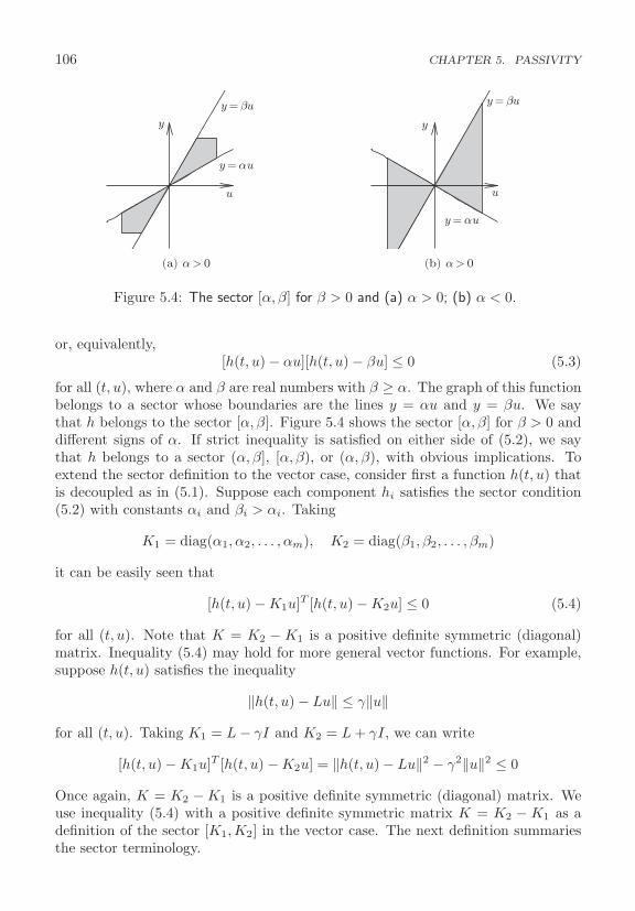
106 CHAPTER 5. PASSIVITY
y = βu
y = αu
y = αu
y = βu
y
u u
y
(b) α > 0(a) α > 0
Figure 5.4: The sector [α, β] for β > 0 and (a) α > 0; (b) α < 0.
or, equivalently,[h(t, u) − αu][h(t, u) − βu] ≤ 0 (5.3)
for all (t, u), where α and β are real numbers with β ≥ α. The graph of this functionbelongs to a sector whose boundaries are the lines y = αu and y = βu. We saythat h belongs to the sector [α, β]. Figure 5.4 shows the sector [α, β] for β > 0 anddifferent signs of α. If strict inequality is satisfied on either side of (5.2), we saythat h belongs to a sector (α, β], [α, β), or (α, β), with obvious implications. Toextend the sector definition to the vector case, consider first a function h(t, u) thatis decoupled as in (5.1). Suppose each component hi satisfies the sector condition(5.2) with constants αi and βi > αi. Taking
K1 = diag(α1, α2, . . . , αm), K2 = diag(β1, β2, . . . , βm)
it can be easily seen that
[h(t, u) − K1u]T [h(t, u) − K2u] ≤ 0 (5.4)
for all (t, u). Note that K = K2 − K1 is a positive definite symmetric (diagonal)matrix. Inequality (5.4) may hold for more general vector functions. For example,suppose h(t, u) satisfies the inequality
‖h(t, u) − Lu‖ ≤ γ‖u‖for all (t, u). Taking K1 = L − γI and K2 = L + γI, we can write
[h(t, u) − K1u]T [h(t, u) − K2u] = ‖h(t, u) − Lu‖2 − γ2‖u‖2 ≤ 0
Once again, K = K2 − K1 is a positive definite symmetric (diagonal) matrix. Weuse inequality (5.4) with a positive definite symmetric matrix K = K2 − K1 as adefinition of the sector [K1,K2] in the vector case. The next definition summariesthe sector terminology.
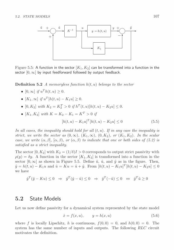
5.2. STATE MODELS 107
+
+
+
−yu u y
y = h(t, u)u
K−1
K1
Figure 5.5: A function in the sector [K1,K2] can be transformed into a function in thesector [0,∞] by input feedforward followed by output feedback.
Definition 5.2 A memoryless function h(t, u) belongs to the sector
• [0,∞] if uT h(t, u) ≥ 0.
• [K1,∞] if uT [h(t, u) − K1u] ≥ 0.
• [0,K2] with K2 = KT2 > 0 if hT (t, u)[h(t, u) − K2u] ≤ 0.
• [K1,K2] with K = K2 − K1 = KT > 0 if
[h(t, u) − K1u]T [h(t, u) − K2u] ≤ 0 (5.5)
In all cases, the inequality should hold for all (t, u). If in any case the inequality isstrict, we write the sector as (0,∞), (K1,∞), (0,K2), or (K1,K2). In the scalarcase, we write (α, β], [α, β), or (α, β) to indicate that one or both sides of (5.2) issatisfied as a strict inequality.
The sector [0,K2] with K2 = (1/δ)I > 0 corresponds to output strict passivity withρ(y) = δy. A function in the sector [K1,K2] is transformed into a function in thesector [0,∞] as shown in Figure 5.5. Define u, u, and y as in the figure. Then,y = h(t, u) − K1u and u = Ku = u + y. From [h(t, u) − K1u]T [h(t, u) − K2u] ≤ 0we have
yT (y − Ku) ≤ 0 ⇒ yT (y − u) ≤ 0 ⇒ yT (−u) ≤ 0 ⇔ yT u ≥ 0
5.2 State Models
Let us now define passivity for a dynamical system represented by the state model
x = f(x, u), y = h(x, u) (5.6)
where f is locally Lipschitz, h is continuous, f(0, 0) = 0, and h(0, 0) = 0. Thesystem has the same number of inputs and outputs. The following RLC circuitmotivates the definition.

108 CHAPTER 5. PASSIVITY
i2v2
vc v3Cv1
y
u
iL
i3i1
++
+
−
−
+
−
+
−−
i3 = h3(v3)i1 = h1(v1)
v2 = h2(i2)L
Figure 5.6: RLC circuit of Example 5.1.
Example 5.1 The RLC circuit of Figure 5.6 features a voltage source connectedto an RLC network with linear inductor and capacitor and nonlinear resistors. Thenonlinear resistors 1 and 3 are represented by their v–i characteristics i1 = h1(v1)and i3 = h3(v3), while resistor 2 is represented by its i–v characteristic v2 = h2(i2).We take the voltage u as the input and the current y as the output. The productuy is the power flow into the network. Taking the current x1 through the inductorand the voltage x2 across the capacitor as the state variables, the state model is
Lx1 = u − h2(x1) − x2, Cx2 = x1 − h3(x2), y = x1 + h1(u)
The new feature of an RLC network over a resistive network is the presence of theenergy-storing elements L and C. The system is passive if the energy absorbed bythe network over any period of time [0, t] is greater than or equal to the change inthe energy stored in the network over the same period; that is,∫ t
0
u(s)y(s) ds ≥ V (x(t)) − V (x(0)) (5.7)
where V (x) = 12Lx2
1 + 12Cx2
2 is the energy stored in the network. If (5.7) holds withstrict inequality, then the difference between the absorbed energy and the change inthe stored energy must be the energy dissipated in the resistors. Since (5.7) musthold for every t ≥ 0, the instantaneous power inequality
u(t)y(t) ≥ V (x(t), u(t)) (5.8)
must hold for all t; that is, the power flow into the network must be greater than orequal to the rate of change of the energy stored in the network. We can investigateinequality (5.8) by calculating the derivative of V along the trajectories of thesystem. We have
V = Lx1x1 + Cx2x2 = x1[u − h2(x1) − x2] + x2[x1 − h3(x2)]= x1[u − h2(x1)] − x2h3(x2)= [x1 + h1(u)]u − uh1(u) − x1h2(x1) − x2h3(x2)= uy − uh1(u) − x1h2(x1) − x2h3(x2)
5.2. STATE MODELS 109
Thus,uy = V + uh1(u) + x1h2(x1) + x2h3(x2)
If h1, h2, and h3 are passive, uy ≥ V and the system is passive. Other possibilitiesare illustrated by four different special cases of the network.
Case 1: If h1 = h2 = h3 = 0, then uy = V and there is no energy dissipation inthe network; that is, the system is lossless.
Case 2: If h2 and h3 are passive, then uy ≥ V + uh1(u). If uh1(u) > 0 for allu �= 0, the energy absorbed over [0, t] will be equal to the change in the storedenergy only when u(t) ≡ 0. This is a case of input strict passivity.
Case 3: If h1 = 0 and h3 is passive, then uy ≥ V + yh2(y). When yh2(y) > 0 forall y �= 0, we have output strict passivity because the energy absorbed over[0, t] will be equal to the change in the stored energy only when y(t) ≡ 0.
Case 4: If h1 ∈ [0,∞], h2 ∈ (0,∞), and h3 ∈ (0,∞), then
uy ≥ V + x1h2(x1) + x2h3(x2)
where x1h2(x1) + x2h3(x2) is a positive definite function of x. This is a caseof state strict passivity because the energy absorbed over [0, t] will be equalto the change in the stored energy only when x(t) ≡ 0. A system having thisproperty is called state strictly passive or, simply, strictly passive.
�
Definition 5.3 The system (5.6) is passive if there exists a continuously differen-tiable positive semidefinite function V (x) (called the storage function) such that
uT y ≥ V =∂V
∂xf(x, u), ∀ (x, u) (5.9)
Moreover, it is
• lossless if uT y = V .
• input strictly passive if uT y ≥ V + uT ϕ(u) and uT ϕ(u) > 0, ∀ u �= 0.
• output strictly passive if uT y ≥ V + yT ρ(y) and yT ρ(y) > 0, ∀ y �= 0.
• strictly passive if uT y ≥ V + ψ(x) for some positive definite function ψ.
In all cases, the inequality should hold for all (x, u).

110 CHAPTER 5. PASSIVITY
u x = y
+u x y
h(.)+
−
u x = y
h(.)
(a) (b) (c)
Figure 5.7: Example 5.2
Example 5.2 The integrator of Figure 5.7(a), represented by
x = u, y = x
is a lossless system since, with V (x) = 12x2 as the storage function, uy = V . When
a memoryless function is connected in parallel with the integrator, as shown inFigure 5.7(b), the system is represented by
x = u, y = x + h(u)
With V (x) = 12x2 as the storage function, uy = V +uh(u). If h ∈ [0,∞], the system
is passive. If uh(u) > 0 for all u �= 0, the system is input strictly passive. When theloop is closed around the integrator with a memoryless function, as in Figure 5.7(c),the system is represented by
x = −h(x) + u, y = x
With V (x) = 12x2 as the storage function, uy = V +yh(y). If h ∈ [0,∞], the system
is passive. If yh(y) > 0 for all y �= 0, the system is output strictly passive. �
Example 5.3 The cascade connection of an integrator and a passive memorylessfunction, shown in Figure 5.8(a), is represented by
x = u, y = h(x)
Passivity of h guarantees that∫ x
0h(σ) dσ ≥ 0 for all x. With V (x) =
∫ x
0h(σ) dσ as
the storage function, V = h(x)x = yu. Hence, the system is lossless. Suppose nowthe integrator is replaced by the transfer function 1/(as + 1) with a > 0, as shownin Figure 5.8(b). The system can be represented by the state model
ax = −x + u, y = h(x)
With V (x) = a∫ x
0h(σ) dσ as the storage function,
V = h(x)(−x + u) = yu − xh(x) ≤ yu
Hence, the system is passive. If xh(x) > 0 ∀ x �= 0, it is strictly passive. �
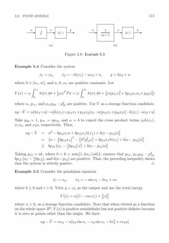
5.2. STATE MODELS 111
1
as + 1
u x yh(.)
u x yh(.)
(a) (b)
Figure 5.8: Example 5.3
Example 5.4 Consider the system
x1 = x2, x2 = −h(x1) − ax2 + u, y = bx2 + u
where h ∈ [α1,∞], and a, b, α1 are positive constants. Let
V (x) = α
∫ x1
0
h(σ) dσ + 12αxT Px = α
∫ x1
0
h(σ) dσ + 12α(p11x
21 +2p12x1x2 +p22x
22)
where α, p11, and p11p22 − p212 are positive. Use V as a storage function candidate.
uy−V = u(bx2+u)−α[h(x1)+p11x1+p12x2]x2−α(p12x1+p22x2)[−h(x1)−ax2+u]
Take p22 = 1, p11 = ap12, and α = b to cancel the cross product terms x2h(x1),x1x2, and x2u, respectively. Then,
uy − V = u2 − bp12x1u + bp12x1h(x1) + b(a − p12)x22
=(u − 1
2bp12x1
)2 − 14b2p2
12x21 + bp12x1h(x1) + b(a − p12)x2
2
≥ bp12
(α1 − 1
4bp12
)x2
1 + b(a − p12)x22
Taking p12 = ak, where 0 < k < min{1, 4α1/(ab)}, ensures that p11, p11p22 − p212,
bp12
(α1 − 1
4bp12
), and b(a−p12) are positive. Thus, the preceding inequality shows
that the system is strictly passive. �Example 5.5 Consider the pendulum equation
x1 = x2, x2 = − sin x1 − bx2 + cu
where b ≥ 0 and c > 0. View y = x2 as the output and use the total energy
V (x) = α[(1 − cos x1) + 12x2
2]
where α > 0, as a storage function candidate. Note that when viewed as a functionon the whole space R2, V (x) is positive semidefinite but not positive definite becauseit is zero at points other than the origin. We have
uy − V = ux2 − α[x2 sin x1 − x2 sin x1 − bx22 + cx2u]
112 CHAPTER 5. PASSIVITY
Taking α = 1/c to cancel the cross product term x2u, we obtain
uy − V = (b/c)x22 ≥ 0
Hence, the system is passive when b = 0 and output strictly passive when b > 0.�
5.3 Positive Real Transfer Functions
Definition 5.4 An m×m proper rational transfer function matrix G(s) is positivereal if
• poles of all elements of G(s) are in Re[s] ≤ 0,
• for all real ω for which jω is not a pole of any element of G(s), the matrixG(jω) + GT (−jω) is positive semidefinite, and
• any pure imaginary pole jω of any element of G(s) is a simple pole and theresidue matrix lims→jω(s − jω)G(s) is positive semidefinite Hermitian.
It is strictly positive real if G(s − ε) is positive real for some ε > 0.
When m = 1, G(jω)+GT (−jω) = 2Re[G(jω)], an even function of ω. Therefore,the second condition of Definition 5.4 reduces to Re[G(jω)] ≥ 0, ∀ ω ∈ [0,∞), whichholds when the Nyquist plot of G(jω) lies in the closed right-half complex plane.This is a condition that can be satisfied only if the relative degree of the transferfunction is zero or one.2
The next lemma gives an equivalent characterization of strictly positive realtransfer functions.3
Lemma 5.1 Let G(s) be an m × m proper rational transfer function matrix, andsuppose det [G(s) + GT (−s)] is not identically zero.4 Then, G(s) is strictly positivereal if and only if
• G(s) is Hurwitz; that is, poles of all elements of G(s) have negative real parts,
• G(jω) + GT (−jω) is positive definite for all ω ∈ R, and
• either G(∞) + GT (∞) is positive definite or it is positive semidefinite andlimω→∞ ω2(m−q) det[G(jω)+GT (−jω)] > 0, where q = rank[G(∞)+GT (∞)].
In the case m = 1, the frequency-domain condition of the lemma reduces toRe[G(jω)] > 0 for all ω ∈ [0,∞) and either G(∞) > 0 or G(∞) = 0 andlimω→∞ ω2Re[G(jω)] > 0.
2The relative degree of a rational transfer function G(s) = n(s)/d(s) is deg d - deg n. For aproper transfer function, the relative degree is a nonnegative integer.
3The proof is given in [30].4Equivalently, G(s) + GT (−s) has a normal rank m over the field of rational functions of s.
5.3. POSITIVE REAL TRANSFER FUNCTIONS 113
Example 5.6 The transfer function G(s) = 1/s is positive real since it has no polesin Re[s] > 0, has a simple pole at s = 0 whose residue is 1, and Re[G(jω)] = 0,∀ ω �= 0. It is not strictly positive real since 1/(s − ε) has a pole in Re[s] > 0for any ε > 0. The transfer function G(s) = 1/(s + a) with a > 0 is positive real,since it has no poles in Re[s] ≥ 0 and Re[G(jω)] = a/(ω2 + a2) > 0, ∀ ω ∈ [0,∞)Since this is so for every a > 0, we see that for any ε ∈ (0, a) the transfer functionG(s − ε) = 1/(s + a − ε) will be positive real. Hence, G(s) = 1/(s + a) is strictlypositive real. The same conclusion can be drawn from Lemma 5.1 by noting that
limω→∞ω2Re[G(jω)] = lim
ω→∞ω2a
ω2 + a2= a > 0
The transfer function G(s) = 1/(s2 + s + 1) is not positive real because its relativedegree is two. We can see it also by calculating
Re[G(jω)] =1 − ω2
(1 − ω2)2 + ω2< 0, ∀ ω > 1
Consider the 2 × 2 transfer function matrix
G(s) =1
s + 1
[s + 1 1−1 2s + 1
]
Since det[G(s) + GT (−s)] is not identically zero, we can apply Lemma 5.1. Notingthat G(∞) + GT (∞) is positive definite and
G(jω) + GT (−jω) =2
ω2 + 1
[ω2 + 1 −jω
jω 2ω2 + 1
]is positive definite for all ω ∈ R, we can conclude that G(s) is strictly positive real.Finally, the 2 × 2 transfer function matrix
G(s) =
⎡⎣ s+2
s+11
s+2
−1s+2
2s+1
⎤⎦ has G(∞) + GT (∞) =
[2 00 0
]
It can be verified that
G(jω) + GT (−jω) =
⎡⎢⎣
2(2+ω2)1+ω2
−2jω4+ω2
2jω4+ω2
41+ω2
⎤⎥⎦
is positive definite for all ω ∈ R and limω→∞ ω2 det[G(jω) + GT (−jω)] = 4. Con-sequently, by Lemma 5.1, we conclude that G(s) is strictly positive real. �
Passivity properties of positive real transfer functions can be shown by using thenext two lemmas, which are known, respectively, as the positive real lemma and the
114 CHAPTER 5. PASSIVITY
Kalman–Yakubovich–Popov lemma.5 The lemmas give algebraic characterization ofpositive real and strictly positive real transfer functions.
Lemma 5.2 (Positive Real) Let G(s) = C(sI−A)−1B+D be an m×m transferfunction matrix where (A,B) is controllable and (A,C) is observable. Then, G(s)is positive real if and only if there exist matrices P = PT > 0, L, and W such that
PA + AT P = −LT L (5.10)PB = CT − LT W (5.11)
WT W = D + DT (5.12)
�
Lemma 5.3 (Kalman–Yakubovich–Popov) Let G(s) = C(sI − A)−1B + D bean m × m transfer function matrix, where (A,B) is controllable and (A,C) is ob-servable. Then, G(s) is strictly positive real if and only if there exist matricesP = PT > 0, L, and W , and a positive constant ε such that
PA + AT P = −LT L − εP (5.13)PB = CT − LT W (5.14)
WT W = D + DT (5.15)
�
Proof of Lemma 5.3: Suppose there exist P = PT > 0, L, W , and ε > 0 thatsatisfy (5.13) through (5.15). Set μ = 1
2ε and recall that G(s − μ) = C(sI − μI −A)−1B + D. From (5.13), we have
P (A + μI) + (A + μI)T P = −LT L (5.16)
It follows from Lemma 5.2 that G(s − μ) is positive real. Hence, G(s) is strictlypositive real. On the other hand, suppose G(s) is strictly positive real. There existsμ > 0 such that G(s − μ) is positive real. It follows from Lemma 5.2 that thereare matrices P = PT > 0, L, and W , which satisfy (5.14) through (5.16). Settingε = 2μ shows that P , L, W , and ε satisfy (5.13) through (5.15). �
Lemma 5.4 The linear time-invariant minimal realization
x = Ax + Bu, y = Cx + Du
with G(s) = C(sI − A)−1B + D is
• passive if G(s) is positive real;
• strictly passive if G(s) is strictly positive real.5The proof of Lemma 5.2 is given in [74, Lemma 6.2].
5.4. CONNECTION WITH STABILITY 115
�
Proof: Apply Lemmas 5.2 and 5.3, respectively, and use V (x) = 12xT Px as the
storage function.
uT y − ∂V
∂x(Ax + Bu) = uT (Cx + Du) − xT P (Ax + Bu)
= uT Cx + 12uT (D + DT )u − 1
2xT (PA + AT P )x − xT PBu
= uT (BT P + WT L)x + 12uT WT Wu
+ 12xT LT Lx + 1
2εxT Px − xT PBu
= 12 (Lx + Wu)T (Lx + Wu) + 1
2εxT Px ≥ 12εxT Px
In the case of Lemma 5.2, ε = 0 and we conclude that the system is passive, while inthe case of Lemma 5.3, ε > 0 and we conclude that the system is strictly passive. �
5.4 Connection with Stability
In this section we consider a passive system of the form
x = f(x, u), y = h(x, u) (5.17)
where f is locally Lipschitz, h is continuous, f(0, 0) = 0, and h(0, 0) = 0, and studythe stability of the origin as an equilibrium point of x = f(x, 0).
Lemma 5.5 If the system (5.17) is passive with a positive definite storage functionV (x), then the origin of x = f(x, 0) is stable.
Proof: Take V as a Lyapunov function candidate for x = f(x, 0). Then V ≤ 0. �
To show asymptotic stability of the origin of x = f(x, 0), we need to either showthat V is negative definite or apply the invariance principle. In the next lemma, weapply the invariance principle by considering a case where V = 0 when y = 0 andthen require the additional property that
y(t) ≡ 0 ⇒ x(t) ≡ 0 (5.18)
for all solutions of (5.17) when u = 0. Equivalently, no solutions of x = f(x, 0) canstay identically in S = {h(x, 0) = 0}, other than the zero solution x(t) ≡ 0. Theproperty (5.18) can be interpreted as an observability condition. Recall that for thelinear system
x = Ax, y = Cx
observability is equivalent to
y(t) = CeAtx(0) ≡ 0 ⇔ x(0) = 0 ⇔ x(t) ≡ 0
For easy reference, we define (5.18) as an observability property of the system.

116 CHAPTER 5. PASSIVITY
Definition 5.5 The system (5.17) is said to be zero-state observable if no solutionof x = f(x, 0) can stay identically in S = {h(x, 0) = 0}, other than the zero solutionx(t) ≡ 0.
Lemma 5.6 Consider the system (5.17). The origin of x = f(x, 0) is asymptoti-cally stable if the system is
• strictly passive or
• output strictly passive and zero-state observable.
Furthermore, if the storage function is radially unbounded, the origin will be globallyasymptotically stable. �
Proof: Suppose the system is strictly passive and let V (x) be its storage function.Then, with u = 0, V satisfies the inequality V ≤ −ψ(x), where ψ(x) is positivedefinite. We can use this inequality to show that V (x) is positive definite. Inparticular, for any x ∈ Rn, the equation x = f(x, 0) has a solution φ(t;x), startingfrom x at t = 0 and defined on some interval [0, δ]. Integrating the inequalityV ≤ −ψ(x) yields
V (φ(τ, x)) − V (x) ≤ −∫ τ
0
ψ(φ(t;x)) dt, ∀ τ ∈ [0, δ]
Using V (φ(τ, x)) ≥ 0, we obtain
V (x) ≥∫ τ
0
ψ(φ(t;x)) dt
Suppose there is x �= 0 such that V (x) = 0. The foregoing inequality implies∫ τ
0
ψ(φ(t; x)) dt = 0, ∀ τ ∈ [0, δ] ⇒ ψ(φ(t; x)) ≡ 0 ⇒ φ(t; x) ≡ 0 ⇒ x = 0
which contradicts the claim that x �= 0. Thus, V (x) > 0 for all x �= 0. This qualifiesV (x) as a Lyapunov function candidate, and since V (x) ≤ −ψ(x), we conclude thatthe origin is asymptotically stable.
Suppose now that the system is output strictly passive and let V (x) be itsstorage function. Then, with u = 0, V satisfies the inequality V ≤ −yT ρ(y), whereyT ρ(y) > 0 for all y �= 0. By repeating the preceding argument, we can use thisinequality to show that V (x) is positive definite. In particular, if there is x �= 0such that V (x) = 0, then
0 = V (x) ≥∫ τ
0
hT (φ(t; x), 0)ρ(h(φ(t; x), 0)) dt, ∀ τ ∈ [0, δ] ⇒ h(φ(t; x), 0) ≡ 0
Due to zero-state observability,
h(φ(t; x), 0) ≡ 0 ⇒ φ(t; x) ≡ 0 ⇒ x = 0
5.4. CONNECTION WITH STABILITY 117
Hence, V (x) > 0 for all x �= 0. Since V (x) ≤ −yT ρ(y) and y(t) ≡ 0 ⇒ x(t) ≡ 0,we conclude by the invariance principle that the origin is asymptotically stable.Finally, if V (x) is radially unbounded, we can infer global asymptotic stability fromTheorems 3.3 and 3.5, respectively. �
Example 5.7 Consider the m-input–m-output system
x = f(x) + G(x)u, y = h(x)
where f and G are locally Lipschitz, h is continuous, f(0) = 0, and h(0) = 0.Suppose there is a continuously differentiable positive semidefinite function V (x)such that
∂V
∂xf(x) ≤ 0,
∂V
∂xG(x) = hT (x)
Then,
uT y − ∂V
∂x[f(x) + G(x)u] = uT h(x) − ∂V
∂xf(x) − hT (x)u = − ∂V
∂xf(x) ≥ 0
which shows that the system is passive. If V (x) is positive definite, we can concludethat the origin of x = f(x) is stable. If we have the stronger condition
∂V
∂xf(x) ≤ −khT (x)h(x),
∂V
∂xG(x) = hT (x)
for some k > 0, then
uT y − ∂V
∂x[f(x) + G(x)u] ≥ kyT y
and the system is output strictly passive with ρ(y) = ky. If, in addition, it is zero-state observable, then the origin of x = f(x) is asymptotically stable. Furthermore,if V (x) is radially unbounded, the origin will be globally asymptotically stable. �Example 5.8 Consider the single-input–single-output system6
x1 = x2, x2 = −ax31 − kx2 + u, y = x2
where a and k are positive constants. Let V (x) = 14ax4
1 + 12x2
2 be a storage functioncandidate.
V = ax31x2 + x2(−ax3
1 − kx2 + u) = −ky2 + yu
Therefore, the system is output strictly passive. Moreover, when u = 0,
y(t) ≡ 0 ⇔ x2(t) ≡ 0 ⇒ ax31(t) ≡ 0 ⇒ x1(t) ≡ 0
Hence, the system is zero-state observable. It follows from Lemma 5.6 that theorigin of the unforced system is globally asymptotically stable. �
6Lyapunov stability of this system was studied in Examples 3.8 and 3.9.
118 CHAPTER 5. PASSIVITY
5.5 Exercises
5.1 Show that the parallel connection of two passive (respectively, input strictlypassive, output strictly passive, strictly passive) dynamical systems is passive (re-spectively, input strictly passive, output strictly passive, strictly passive).
5.2 Consider the system
x1 = −ax1 + x2, x2 = −h(x1) − bx2 + u, y = x2
where a ≥ 0, b ≥ 0, h is locally Lipschitz, h(0) = 0 and x1h(x1) > 0 for allx1 �= 0. Using a storage function of the form V (x) = k1
∫ x1
0h(σ) dσ + 1
2k2x22, with
appropriately chosen positive constants k1 and k2, show that the system is
(a) Passive.
(b) Lossless when a = b = 0.
(c) Output strictly passive when b > 0.
(d) Strictly passive when a > 0 and b > 0.
5.3 Consider the system
x1 = x2, x2 = −g(x1)(x1 + x2) + u, y = x1 + 2x2
where g is locally Lipschitz and g(y) ≥ 1 for all y. Using the storage functionV (x) =
∫ x1
0σg(σ) dσ +
∫ x2
0(x1 + 2σ) dσ, show that the system is passive.
5.4 Consider the system
x1 = x2, x2 = −h(x1) − ax2 + u, y = bx1 + cx2
where a, b, c are positive constants, h is locally Lipschitz, h(0) = 0 and x1h(x1) > 0for all x1 �= 0. Using a storage function of the form V (x) = k
∫ x1
0h(σ) dσ + 1
2xT Px,with appropriately chosen positive constant k and positive definite matrix P , showthat the system is strictly passive if b < ac.
5.5 Consider the system
x1 = x2, x2 = −h1(x1) − x2 − h2(x3) + u, x3 = x2 − x3, y = x2
where h1 and h2 are locally Lipschitz functions that satisfy hi(0) = 0 and yhi(y) > 0for all y �= 0. Using a storage function of the form V (x) = k1
∫ x1
0h1(σ) dσ +k2x
22 +
k3
∫ x3
0h2(σ) dσ, with appropriately chosen positive constants k1 to k3, show that
the system is output strictly passive.

5.5. EXERCISES 119
5.6 Consider the system
Mx = −Kx + ah(x) + u, y = h(x)
where x, u, and y are n-dimensional vectors, M and K are positive definite sym-metric matrices, h is locally Lipschitz, h ∈ [0,K], and
∫ x
0hT (σ)M dσ ≥ 0 for all
x. Show that the system is passive when a = 1 and output strictly passive whena < 1.
5.7 For each of the following systems, show the stated passivity property for thegiven output.
(1) The mass-spring system (A.6) with y = x2 is output strictly passive.
(2) The tunnel-diode circuit (A.7) with y = x2 is strictly passive.
(3) The boost converter (A.16) with y = k(x1 − αkx2) is passive.
5.8 An m-link robot manipulator is represented by equation (A.34). Supposeg(q) = 0 has an isolated solution q = q∗ and the potential energy P (q) has aminimum at q∗; that is, P (q) ≥ P (q∗) for all q.
(a) Using V = 12 qT M(q)q + P (q) − P (q∗) as a storage function candidate, show
that the system, with input u and output q, is passive.
(b) Let u = −Kdq + v, where Kd is a positive definite symmetric matrix. Showthat the system, with input v and output q, is output strictly passive.
5.9 ([105]) Euler equations for a rotating rigid spacecraft are given by
J1ω1 = (J2−J3)ω2ω3+u1, J2ω2 = (J3−J1)ω3ω1+u2, J3ω3 = (J1−J2)ω1ω2+u3
where ω = col(ω1, ω2, ω3) is the angular velocity vector along the principal axes,u = col(u1, u2, u3) is the vector of torque inputs applied about the principal axes,and J1 to J3 are the principal moments of inertia.
(a) Show that the system, with input u and output ω, is lossless.
(b) Let u = −Kω + v, where K is a positive definite symmetric matrix. Show thatthe system, with input v and output ω, is strictly passive.
5.10 Consider the TORA system of Section A.12.
(a) Using the sum of the potential energy 12kx2
c and kinetic energy 12vT Dv, where
v =[
θxc
]and D =
[J + mL2 mL cos θmL cos θ m + M
]
as the storage function, show that the system with input u and output θ ispassive.
120 CHAPTER 5. PASSIVITY
(b) Let u = −φ1(θ) + w where φ1 is locally Lipschitz, φ1(0) = 0 and yφ1(y) > 0for all y �= 0. Using
V =12vT Dv +
12kx2
c +∫ θ
0
φ1(λ) dλ
as the storage function, show that the system with input w and output θ ispassive.
5.11 Show that the transfer function (b1s + b2)/(s2 + a1s + a2) is strictly positivereal if and only if all coefficients are positive and b2 < a1b1.
5.12 Show that the transfer function d + b1s/(s2 + a1s + a2) is strictly positivereal if a1, a2, d, and a1d + b1 are positive.
5.13 Consider the system
x =[
0 1−1 −1
]x +[01
]u, y =
[1 2
]x
(a) Find the transfer function and show that it is strictly positive real.
(b) Choose ε such that A + (ε/2)I is Hurwitz and solve equations (5.13) through(5.15) for P , L and W .
5.14 Consider equations (5.13) through (5.15) and suppose that (D +DT ) is non-singular. Choose ε such that A + (ε/2)I is Hurwitz. Show that P satisfies theRiccati equation7
PA0 + AT0 P − PB0P + C0 = 0
where A0 = −(ε/2)I − A + B(D + DT )−1C, B0 = B(D + DT )−1BT , and C0 =−CT (D + DT )−1C, and L is given by
LT L = (CT − PB)(D + DT )−1(C − BT P )
5.15 Investigate zero-state observability of the systems in the following exercises:
5.2 5.3 5.4 5.55.6 5.7(1) 5.7(2) 5.7(3)5.8(a) 5.8(b) 5.10(a) 5.10(b)
7The Riccati equation can be solved by the MATLAB command “are(A0, B0, C0)”.
Chapter 6
Input-Output Stability
input-output stability In most of this book, we use the state-space approach tomodel nonlinear dynamical systems and place a lot of emphasis on the behaviorof the state variables. An alternative approach to the mathematical modeling ofdynamical systems is the input-output approach. An input-output model relatesthe output of the system directly to the input, with no knowledge of the internalstructure that is represented by the state equation. The system is viewed as a blackbox that can be accessed only through its input and output terminals. The input-output approach can handle systems that are not representable by state modelssuch as systems with time delay, which cannot be represented by state models unlessthe system is approximated. This chapter gives a brief introduction to the notionof input-output stability and how to show it for state models.1 In Section 6.1,we introduce input-output models and define L stability, a notion of stability inthe input-output sense. In Section 6.2, we study L stability of nonlinear systemsrepresented by state models. Finally, in Section 6.3 we discuss the calculation ofthe L2 gain for a special class of nonlinear systems.
6.1 L Stability
We consider a system whose input–output relation is represented by
y = Hu
where H is some mapping or operator that specifies y in terms of u. The input ubelongs to a space of signals that map the time interval [0,∞) into the Euclideanspace Rm; that is, u : [0,∞) → Rm. Examples are the space of piecewise con-tinuous, bounded functions; that is, supt≥0 ‖u(t)‖ < ∞, and the space of piecewise
1For comprehensive treatment of input-output stability, the reader may consult [35, 116, 147].
121
122 CHAPTER 6. INPUT-OUTPUT STABILITY
continuous, square-integrable functions; that is,∫∞0
uT (t)u(t) dt < ∞. To mea-sure the size of a signal, we introduce the norm function ‖u‖, which satisfies threeproperties:
• The norm of a signal is zero if and only if the signal is identically zero and isstrictly positive otherwise.
• Scaling a signal results in a corresponding scaling of the norm; that is, ‖au‖ =a‖u‖ for any positive constant a and every signal u.
• The norm satisfies the triangle inequality ‖u1 + u2‖ ≤ ‖u1‖ + ‖u2‖ for anysignals u1 and u2.
For the space of piecewise continuous, bounded functions, the norm is defined as
‖u‖L∞ = supt≥0
‖u(t)‖ < ∞
and the space is denoted by Lm∞. For the space of piecewise continuous, square-
integrable functions, the norm is defined by
‖u‖L2 =
√∫ ∞
0
uT (t)u(t) dt < ∞
and the space is denoted by Lm2 . More generally, the space Lm
p for 1 ≤ p < ∞ isdefined as the set of all piecewise continuous functions u : [0,∞) → Rm such that
‖u‖Lp=(∫ ∞
0
‖u(t)‖p dt
)1/p
< ∞
The subscript p in Lmp refers to the type of p-norm used to define the space, while
the superscript m is the dimension of the signal u. If they are clear from the context,we may drop one or both of them and refer to the space simply as Lp, Lm, or L.To distinguish the norm of u as a vector in the space L from the norm of u(t) as avector in Rm, we write the first norm as ‖ · ‖L.
If we think of u ∈ Lm as a “well-behaved” input, the question to ask is whetherthe output y will be “well behaved” in the sense that y ∈ Lq, where Lq is the samespace as Lm, except that q (the number of output variables) could be differentfrom m (the number of input variables). A system having the property that any“well-behaved” input will generate a “well-behaved” output will be defined as astable system. However, we cannot define H as a mapping from Lm to Lq, becausewe have to deal with systems which are unstable, in that an input u ∈ Lm maygenerate an output y that does not belong to Lq. Therefore, H is usually definedas a mapping from an extended space Lm
e to an extended space Lqe, where Lm
e isdefined by
Lme = {u | uτ ∈ Lm,∀ τ ∈ [0,∞)}

6.1. L STABILITY 123
and uτ is a truncation of u defined by
uτ (t) ={
u(t), 0 ≤ t ≤ τ0, t > τ
The extended space Lme is a linear space that contains the unextended space Lm as
a subset. It allows us to deal with unbounded “ever-growing” signals. For example,the signal u(t) = t does not belong to the space L∞, but its truncation
uτ (t) ={
t, 0 ≤ t ≤ τ0, t > τ
belongs to L∞ for every finite τ . Hence, u(t) = t belongs to the extended spaceL∞e.
A mapping H : Lme → Lq
e is said to be causal if the value of the output (Hu)(t)at any time t depends only on the values of the input up to time t. This is equivalentto
(Hu)τ = (Huτ )τ
Causality is an intrinsic property of dynamical systems represented by state models.With the space of input and output signals defined, we proceed to define input–
output stability. We start by defining the concept of a gain function.
Definition 6.1 A scalar continuous function g(r), defined for r ∈ [0, a), is a gainfunction if it is nondecreasing and g(0) = 0.
Note that a class K function is a gain function but not the other way around.By not requiring the gain function to be strictly increasing we can have g = 0 org(r) = sat(r).
Definition 6.2 A mapping H : Lme → Lq
e is L stable if there exist a gain functiong, defined on [0,∞), and a nonnegative constant β such that
‖(Hu)τ‖L ≤ g (‖uτ‖L) + β (6.1)
for all u ∈ Lme and τ ∈ [0,∞). It is finite-gain L stable if there exist nonnegative
constants γ and β such that
‖(Hu)τ‖L ≤ γ‖uτ‖L + β (6.2)
for all u ∈ Lme and τ ∈ [0,∞).
The constant β in (6.1) or (6.2) is called the bias term. It is included in the definitionto allow for systems where Hu does not vanish at u = 0. When inequality (6.2) issatisfied, we say that the system has L gain ≤ γ.
For causal, L stable systems, it can be shown by a simple argument that
u ∈ Lm ⇒ Hu ∈ Lq

124 CHAPTER 6. INPUT-OUTPUT STABILITY
and‖Hu‖L ≤ g (‖u‖L) + β, ∀ u ∈ Lm
For causal, finite-gain L stable systems, the foregoing inequality takes the form
‖Hu‖L ≤ γ‖u‖L + β, ∀ u ∈ Lm
The definition of L∞ stability is the familiar notion of bounded-input–bounded-output stability; namely, if the system is L∞ stable, then for every bounded inputu(t), the output Hu(t) is bounded.
Example 6.1 a real-valued function of a real argument h(u) can be viewed as anoperator H that assigns to every input signal u(t) the output signal y(t) = h(u(t)).We use this simple operator to illustrate the definition of L stability. Suppose
|h(u)| ≤ a + b|u|, ∀ u ∈ R
Then, H is finite-gain L∞ stable with γ = b and β = a. If a = 0, then for eachp ∈ [1,∞), ∫ ∞
0
|h(u(t))|p dt ≤ (b)p
∫ ∞
0
|u(t)|p dt
Thus, for each p ∈ [1,∞], the operator H is finite-gain Lp stable with zero bias andγ = b. Finally, for h(u) = u2, H is L∞ stable with zero bias and g(r) = r2. It isnot finite-gain L∞ stable because |h(u)| = u2 cannot be bounded γ|u| + β for allu ∈ R. �
Example 6.2 Consider a single-input–single-output system defined by the causalconvolution operator
y(t) =∫ t
0
h(t − σ)u(σ) dσ
where h(t) = 0 for t < 0. Suppose h ∈ L1e; that is, for every τ ∈ [0,∞),
‖hτ‖L1 =∫ ∞
0
|hτ (σ)| dσ =∫ τ
0
|h(σ)| dσ < ∞
If u ∈ L∞e and τ ≥ t, then
|y(t)| ≤∫ t
0
|h(t − σ)| |u(σ)| dσ
≤∫ t
0
|h(t − σ)| dσ sup0≤σ≤τ
|u(σ)| =∫ t
0
|h(s)| ds sup0≤σ≤τ
|u(σ)|
Consequently,‖yτ‖L∞ ≤ ‖hτ‖L1‖uτ‖L∞ , ∀ τ ∈ [0,∞)
6.1. L STABILITY 125
This inequality resembles (6.2), but it is not the same as (6.2) because the constantγ in (6.2) is required to be independent of τ . While ‖hτ‖L1 is finite for every finite τ ,it may not be bounded uniformly in τ . For example, h(t) = et has ‖hτ‖L1 = (eτ−1),which is finite for all τ ∈ [0,∞) but not uniformly bounded in τ . Inequality (6.2)will be satisfied if h ∈ L1; that is,
‖h‖L1 =∫ ∞
0
|h(σ)| dσ < ∞
Then, the inequality
‖yτ‖L∞ ≤ ‖h‖L1‖uτ‖L∞ , ∀ τ ∈ [0,∞)
shows that the system is finite-gain L∞ stable. The condition ‖h‖L1 < ∞ actuallyguarantees finite-gain Lp stability for each p ∈ [1,∞]. Consider first the case p = 1.For t ≤ τ < ∞, we have∫ τ
0
|y(t)| dt =∫ τ
0
∣∣∣∣∫ t
0
h(t − σ)u(σ) dσ
∣∣∣∣ dt ≤∫ τ
0
∫ t
0
|h(t − σ)| |u(σ)| dσ dt
Reversing the order of integration yields∫ τ
0
|y(t)| dt ≤∫ τ
0
|u(σ)|∫ τ
σ
|h(t − σ)| dt dσ ≤∫ τ
0
|u(σ)| ‖h‖L1 dσ ≤ ‖h‖L1‖uτ‖L1
Thus,‖yτ‖L1 ≤ ‖h‖L1‖uτ‖L1 , ∀ τ ∈ [0,∞)
Consider now the case p ∈ (1,∞) and let q ∈ (1,∞) be defined by 1/p + 1/q = 1.For t ≤ τ < ∞, we have
|y(t)| ≤∫ t
0
|h(t − σ)| |u(σ)| dσ =∫ t
0
|h(t − σ)|1/q|h(t − σ)|1/p|u(σ)| dσ
By Holder’s inequality,2
|y(t)| ≤(∫ t
0
|h(t − σ)| dσ
)1/q (∫ t
0
|h(t − σ)| |u(σ)|p dσ
)1/p
≤ (‖hτ‖L1)1/q
(∫ t
0
|h(t − σ)| |u(σ)|p dσ
)1/p
2Holder’s inequality states that if f ∈ Lpe and g ∈ Lqe, where p ∈ (1,∞) and 1/p + 1/q = 1,then ∫ τ
0|f(t)g(t)| dt ≤
(∫ τ
0|f(t)|p dt
)1/p (∫ τ
0|g(t)|q dt
)1/q
for every τ ∈ [0,∞). (See [7].)
126 CHAPTER 6. INPUT-OUTPUT STABILITY
Thus,
(‖yτ‖Lp
)p =∫ τ
0
|y(t)|p dt
≤∫ τ
0
(‖hτ‖L1)p/q
(∫ t
0
|h(t − σ)| |u(σ)|p dσ
)dt
= (‖hτ‖L1)p/q∫ τ
0
∫ t
0
|h(t − σ)| |u(σ)|p dσ dt
By reversing the order of integration, we obtain
(‖yτ‖Lp
)p ≤ (‖hτ‖L1)p/q∫ τ
0
|u(σ)|p∫ τ
σ
|h(t − σ)| dt dσ
≤ (‖hτ‖L1)p/q ‖hτ‖L1
(‖uτ‖Lp
)p = (‖hτ‖L1)p (‖uτ‖Lp
)pHence,
‖yτ‖Lp≤ ‖h‖L1‖uτ‖Lp
In summary, if ‖h‖L1 < ∞, then for each p ∈ [1,∞], the causal convolution operatoris finite-gain Lp stable and (6.2) is satisfied with γ = ‖h‖L1 and β = 0. �
One drawback of Definition 6.2 is the implicit requirement that inequality (6.1)or (6.2) be satisfied for all signals in the input space Lm. This excludes systemswhere the input–output relation may be defined only for a subset of the input space.The next example explores this point and motivates the definition of small-signalL stability that follows the example.
Example 6.3 Consider a single-input–single-output system defined by y = tan u.The output y(t) is defined only when the input signal is restricted to |u(t)| < π/2for all t ≥ 0. Thus, the system is not L∞ stable in the sense of Definition 6.2.However, if we restrict u(t) to the set |u| ≤ r < π/2, then
|y| ≤(
tan r
r
)|u|
and the system will satisfy the inequality
‖y‖Lp≤(
tan r
r
)‖u‖Lp
for every u ∈ Lp such that |u(t)| ≤ r for all t ≥ 0, where p could be any numberin [1,∞]. In the space L∞, the requirement |u(t)| ≤ r implies that ‖u‖L∞ ≤ r,showing that the foregoing inequality holds only for input signals of small norm.However, for other Lp spaces with p < ∞ the instantaneous bound on |u(t)| doesnot necessarily restrict the norm of the input signal. For example, the signal
u(t) = re−rt/a, a > 0
6.2. L STABILITY OF STATE MODELS 127
which belongs to Lp for each p ∈ [1,∞], satisfies the instantaneous bound |u(t)| ≤ rwhile its Lp norm
‖u‖Lp= r
(a
rp
)1/p
, 1 ≤ p < ∞
can be arbitrarily large. �
Definition 6.3 A mapping H : Lme → Lq
e is small-signal L stable (respectively,small-signal finite-gain L stable ) if there is a positive constant r such that inequality(6.1) [respectively, (6.2)] is satisfied for all u ∈ Lm
e with sup0≤t≤τ ‖u(t)‖ ≤ r.
6.2 L Stability of State Models
The notion of input–output stability is intuitively appealing. This is probablywhy most of us were introduced to dynamical system stability in the frameworkof bounded-input–bounded-output stability. Since, in Lyapunov stability, we put alot of emphasis on studying the stability of equilibrium points and the asymptoticbehavior of state variables, one may wonder: What can we see about input–outputstability starting from the formalism of Lyapunov stability? In this section, weshow how Lyapunov stability tools can be used to establish L stability of nonlinearsystems represented by state models.
Consider the system
x = f(x, u), y = h(x, u) (6.3)
where x(0) = x0, f is locally Lipschitz and h is continuous for all x ∈ D andu ∈ Du, in which D ⊂ Rn is a domain that contains x = 0, and Du ⊂ Rm is adomain that contains u = 0. The dimension q of the output y could be differentfrom the dimension m of the input u. For each fixed x0 ∈ D, the state model(6.3) defines an operator H that assigns to each input signal u(t) the correspondingoutput signal y(t). Suppose x = 0 is an equilibrium point of the unforced system
x = f(x, 0) (6.4)
The theme of this section is that if the origin of (6.4) is asymptotically (or expo-nentially) stable, then, under some assumptions on f and h, the system (6.3) willbe L stable or small-signal L stable for a certain signal space L. We pursue thisidea first in the case of exponentially stability, and then for the more general caseof asymptotic stability.
Theorem 6.1 Consider the system (6.3) and take r > 0 and ru > 0 such that{‖x‖ ≤ r} ⊂ D and {‖u‖ ≤ ru} ⊂ Du. Suppose the following assumptions hold forall x ∈ D and u ∈ Du:

128 CHAPTER 6. INPUT-OUTPUT STABILITY
• x = 0 is an exponentially stable equilibrium point of x = f(x, 0), and there isa Lyapunov function V(x) that satisfies
c1‖x‖2 ≤ V (x) ≤ c2‖x‖2,∂V
∂xf(x, 0) ≤ −c3‖x‖2,
∥∥∥∥∂V
∂x
∥∥∥∥ ≤ c4‖x‖ (6.5)
for some positive constants c1 to c4.
• f and h satisfy the inequalities
‖f(x, u) − f(x, 0)‖ ≤ L‖u‖ (6.6)
‖h(x, u)‖ ≤ η1‖x‖ + η2‖u‖ (6.7)
for some nonnegative constants L, η1, and η2.
Then, for each x0 with ‖x0‖ ≤ r√
c1/c2, the system (6.3) is small-signal finite-gainLp stable for each p ∈ [1,∞]. In particular, for each u ∈ Lpe with sup0≤t≤τ ‖u(t)‖ ≤min{ru, c1c3r/(c2c4L)}, the output y(t) satisfies
‖yτ‖Lp≤ γ‖uτ‖Lp
+ β (6.8)
for all τ ∈ [0,∞), with
γ = η2 +η1c2c4L
c1c3, β = η1ρ‖x0‖
√c2
c1, where ρ =
⎧⎪⎨⎪⎩
1, if p = ∞(
2c2c3p
)1/p
, if p ∈ [1,∞)
Furthermore, if the origin is globally exponentially stable and the assumptions holdglobally (with D = Rn and Du = Rm), then, for each x0 ∈ Rn, the system (6.3) isfinite-gain Lp stable for each p ∈ [1,∞] and (6.8) is satisfied for each u ∈ Lpe. �
Proof: The derivative of V along the trajectories of x = f(x, u) satisfies
V =∂V
∂xf(x, 0) +
∂V
∂x[f(x, u) − f(x, 0)]
≤ −c3‖x‖2 + c4L‖x‖ ‖u‖ ≤ − c3
c2V +
c4L√c1
‖u‖√
V
Let W (x) =√
V (x). When V (x(t)) �= 0, W is given by
W =V
2√
V≤ − c3
2c2W +
c4L
2√
c1‖u‖ (6.9)
When V (x(t)) = 0, W has a directional derivative that satisfies3
W = limδ→0
1δ
[W (x(t + δ)) − W (x(t))] ≤ c4L
2√
c1‖u‖
3See Exercises 3.24 and 5.6 of [74] for how to show this inequality.
6.2. L STABILITY OF STATE MODELS 129
Thus, inequality (6.9) holds all the time. Rewrite it as
W ≤ −aW + b‖u‖where a = c3/(2c2) and b = c4L/(2
√c1). Set U(t) = eatW (x(t)). Then,
U = eatW + aeatW ≤ −aeatW + beat‖u‖ + aeatW = beat‖u‖By integration, we obtain
U(t) ≤ U(0) +∫ t
0
beaτ‖u(τ)‖ dτ
Hence,
W (x(t)) ≤ e−atW (x(0)) +∫ t
0
e−a(t−τ)b‖u(τ)‖ dτ
Recalling that √c1‖x‖ ≤ W (x) ≤ √
c2‖x‖and substituting for b we arrive at
‖x(t)‖ ≤√
c2
c1‖x0‖e−at +
c4L
2c1
∫ t
0
e−a(t−τ)‖u(τ)‖ dτ (6.10)
It can be verified that
‖x0‖ ≤ r
√c1
c2and sup
0≤σ≤t‖u(σ)‖ ≤ c1c3r
c2c4L
ensure that ‖x(t)‖ ≤ r; hence, x(t) stays within the domain of validity of theassumptions. Using (6.7), we have
‖y(t)‖ ≤ k1e−at + k2
∫ t
0
e−a(t−τ)‖u(τ)‖ dτ + k3 ‖u(t)‖
where
k1 =√
c2
c1‖x0‖η1, k2 =
c4Lη1
2c1, k3 = η2
Set
y1(t) = k1e−at, y2(t) = k2
∫ t
0
e−a(t−τ)‖u(τ)‖ dτ, y3(t) = k3 ‖u(t)‖
Suppose now that u ∈ Lmpe for some p ∈ [1,∞]. It is clear that ‖y3τ‖Lp
≤ k3‖uτ‖Lp
and using the results of Example 6.2, it can be verified that ‖y2τ‖Lp≤ (k2/a)‖uτ‖Lp
.As for the first term, y1(t), it can be verified that
‖y1τ‖Lp≤ k1ρ, where ρ =
⎧⎪⎨⎪⎩
1, if p = ∞(
1ap
)1/p
, if p ∈ [1,∞)
130 CHAPTER 6. INPUT-OUTPUT STABILITY
Thus, by the triangle inequality, (6.8) is satisfied with
γ = k3 +k2
a, β = k1ρ
When all the assumptions hold globally, there is no need to restrict ‖x0‖ or ‖u(t)‖.Therefore, (6.8) is satisfied for each x0 ∈ Rn and u ∈ Lpe. �
The use of (the converse Lyapunov) Theorem 3.8 shows the existence of a Lya-punov function satisfying (6.5). Consequently, we have the following corollary.
Corollary 6.1 Suppose that, in some neighborhood of (x = 0, u = 0), f is contin-uously differentiable and h satisfies (6.7). If the origin x = 0 is an exponentiallystable equilibrium point of x = f(x, 0), then there is a constant r0 > 0 such thatfor each x0 with ‖x0‖ < r0, the system (6.3) is small-signal finite-gain Lp stablefor each p ∈ [1,∞]. Furthermore, if all the assumptions hold globally, the origin isglobally exponentially stable, and f is globally Lipschitz, then for each x0 ∈ Rn, thesystem (6.3) is finite-gain Lp stable for each p ∈ [1,∞]. �
Example 6.4 Consider the system
x = −x − x3 + u, y = tanhx + u
with x(0) = x0. The origin of x = −x − x3 is globally exponentially stable, ascan be seen by the Lyapunov function V (x) = 1
2x2. The function V satisfies (6.5)globally with c1 = c2 = 1
2 , c3 = c4 = 1. The functions f and h satisfy (6.6) and(6.7) globally with L = η1 = η2 = 1. Hence, for each x0 ∈ R and each p ∈ [1,∞],the system is finite-gain Lp stable. �
Example 6.5 Consider the system
x1 = x2, x2 = −x1 − x2 − a tanh x1 + u, y = x1
where a is a nonnegative constant. Use
V (x) = xT Px = p11x21 + 2p12x1x2 + p22x
22
as a Lyapunov function candidate for the unforced system:
V = −2p12(x21+ax1 tanhx1)+2(p11−p12−p22)x1x2−2ap22x2 tanh x1−2(p22−p12)x2
2
Choose p11 = p12 + p22 to cancel the cross-product term x1x2. Then, taking p22 =2p12 = 1 makes P positive definite and results in
V = −x21 − x2
2 − ax1 tanhx1 − 2ax2 tanhx1

6.2. L STABILITY OF STATE MODELS 131
Using the fact that x1 tanhx1 ≥ 0 and | tanh x1| ≤ |x1| for all x1, we obtain
V ≤ −‖x‖2 + 2a|x1| |x2| ≤ −(1 − a)‖x‖2
Thus, for all a < 1, V satisfies (6.5) globally with c1 = λmin(P ), c2 = λmax(P ),c3 = 1 − a, and c4 = 2‖P‖ = 2λmax(P ). The functions f and h satisfy (6.6)and (6.7) globally with L = η1 = 1, η2 = 0. Hence, for each x0 ∈ R2 and eachp ∈ [1,∞], the system is finite-gain Lp stable and the Lp gain can be estimated byγ = 2[λmax(P )]2/[(1 − a)λmin(P )]. �
We turn now to the more general case when the origin of x = f(x, 0) is asymp-totically stable and restrict our attention to the study of L∞ stability. The next twotheorems give conditions for L∞ stability and small-signal L∞ stability, respectively.
Theorem 6.2 Consider the system (6.3) and suppose that, for all (x, u), f is locallyLipschitz and h is continuous and satisfies the inequality
‖h(x, u)‖ ≤ g1(‖x‖) + g2(‖u‖) + η (6.11)
for some gain functions g1, g2 and a nonnegative constant η. If the system x =f(x, u) is input-to-state stable, then, for each x0 ∈ Rn, the system (6.3) is L∞stable. �
Proof: Input-to-state stability shows that ‖x(t)‖ satisfies the inequality
‖x(t)‖ ≤ max{
β(‖x0‖, t), γ(
sup0≤σ≤t
‖u(σ)‖)}
(6.12)
for all t ≥ 0, where β and γ are class KL and class K functions, respectively. Using(6.11), we obtain
‖y(t)‖ ≤ g1
(max
{β(‖x0‖, t), γ
(sup
0≤σ≤t‖u(σ)‖
)})+ g2(‖u(t)‖) + η
≤ g1 (β(‖x0‖, t)) + g1
(γ
(sup
0≤σ≤t‖u(σ)‖
))+ g2(‖u(t)‖) + η
where we used the property g1(max{a, b}) ≤ g1(a)+g1(b), which holds for any gainfunction. Thus,
‖yτ‖L∞ ≤ g (‖uτ‖L∞) + β0 (6.13)
for all τ ∈ [0,∞), where g = g1 ◦ γ + g2 and β0 = g1(β(‖x0‖, 0)) + η. �
Theorem 6.3 Consider the system (6.3), where f is locally Lipschitz and h iscontinuous in some neighborhood of (x = 0, u = 0). If the origin of x = f(x, 0)is asymptotically stable, then there is a constant k > 0 such that for any x0 with‖x0‖ < k, the system (6.3) is small-signal L∞ stable. �
132 CHAPTER 6. INPUT-OUTPUT STABILITY
Proof: By Lemma 4.7, the system (6.3) is locally input-to state stable. Hence,there exist positive constants k and k1 such that inequality (6.12) is satisfied forall ‖x(0)‖ ≤ k and ‖u(t)‖ ≤ k1. By continuity of h, inequality (6.11) is satisfied insome neighborhood of (x = 0, u = 0). The rest of the proof is the same as that ofTheorem 6.2. �
Example 6.6 Consider the system
x = −x − 2x3 + (1 + x2)u2, y = x2 + u
We saw in Example 4.13 that the state equation is input-to-state stable. The outputfunction h satisfies (6.11) globally with g1(r) = r2, g2(r) = r, and η = 0. Thus, thesystem is L∞ stable. �
Example 6.7 Consider the system
x1 = −x31 + x2, x2 = −x1 − x3
2 + u, y = x1 + x2
Taking V = (x21 + x2
2), we have
V = −2x41 − 2x4
2 + 2x2u
Using x41 + x4
2 ≥ 12‖x‖4 yields
V ≤ −‖x‖4 + 2‖x‖|u|= −(1 − θ)‖x‖4 − θ‖x‖4 + 2‖x‖|u|, 0 < θ < 1
≤ −(1 − θ)‖x‖4, ∀ ‖x‖ ≥(
2|u|θ
)1/3
Thus, V satisfies inequalities (4.36) and (4.37) of Theorem 4.6 globally, with α1(r) =α2(r) = r2, W3(x) = (1−θ)‖x‖4, and ρ(r) = (2r/θ)1/3. Hence, the state equation isinput-to-state stable. Furthermore, the function h = x1+x2 satisfies (6.11) globallywith g1(r) =
√2r, g2 = 0, and η = 0. Thus, the system is L∞ stable. �
6.3 L2 Gain
L2 stability plays a special role in system analysis. It is natural to work with square-integrable signals, which can be viewed as finite-energy signals.4 In many controlproblems,5 the system is represented as an input–output map, from a disturbanceinput u to a controlled output y, which is required to be small. With L2 inputsignals, the control system is designed to make the input–output map finite-gain
4If you think of u(t) as current or voltage, then uT (t)u(t) is proportional to the instantaneouspower of the signal, and its integral over time is a measure of the energy content of the signal.
5See the literature on H∞ control; for example, [14], [37], [41], [68], [143], or [154].
6.3. L2 GAIN 133
L2 stable and to minimize the L2 gain. In such problems, it is important not onlyto be able to find out that the system is finite-gain L2 stable, but also to calculatethe L2 gain or an upper bound on it. In this section, we show how to calculate anupper bound on the L2 gain for special cases. We start with linear systems.
Theorem 6.4 Consider the linear system
x = Ax + Bu, y = Cx + Du
where A is Hurwitz. Let G(s) = C(sI − A)−1B + D. Then, the L2 gain of thesystem is less than or equal to supω∈R ‖G(jω)‖.6 �
Proof: Due to linearity, we set x(0) = 0. From Fourier transform theory,7 we knowthat for a causal signal u ∈ L2, the Fourier transform U(jω) is given by
U(jω) =∫ ∞
0
u(t)e−jωt dt and Y (jω) = G(jω)U(jω)
Using Parseval’s theorem,8 we can write
‖y‖2L2
=∫ ∞
0
yT (t)y(t) dt =12π
∫ ∞
−∞Y ∗(jω)Y (jω) dω
=12π
∫ ∞
−∞U∗(jω)GT (−jω)G(jω)U(jω) dω
≤(
supω∈R
‖G(jω)‖)2 1
2π
∫ ∞
−∞U∗(jω)U(jω) dω
=(
supω∈R
‖G(jω)‖)2
‖u‖2L2
which shows that the L2 gain is less than or equal to supω∈R ‖G(jω)‖. �
It can be shown that supω∈R ‖G(jω)‖ is indeed the L2 gain and not just anupper bound on it.9 For nonlinear systems, we have two results, Theorems 6.5 and6.6, for estimating the L2 gain. Both theorems make use of the following lemma.
6This is the induced 2-norm of the complex matrix G(jω), which is equal to√λmax[GT (−jω)G(jω)] = σmax[G(jω)]. This quantity is known as the H∞ norm of G(jω) when
G(jω) is viewed as an element of the Hardy space H∞. (See [41].)7See [35].8Parseval’s theorem [35] states that for a causal signal y ∈ L2,
∫ ∞
0yT (t)y(t) dt =
1
2π
∫ ∞
−∞Y ∗(jω)Y (jω) dω
9See [74, Theorem 5.4].

134 CHAPTER 6. INPUT-OUTPUT STABILITY
Lemma 6.1 Consider the multiinput–multioutput system
x = f(x, u), y = h(x, u) (6.14)
where x(0) = x0, f(0, 0) = 0, h(0, 0) = 0, f is locally Lipschitz and h is continuousfor all x ∈ Rn and u ∈ Rm. Let V (x) be a continuously differentiable, positivesemidefinite function such that
V =∂V
∂xf(x, u) ≤ k(γ2‖u‖2 − ‖y‖2) (6.15)
for all (x, u), for some positive constants k and γ. Then, for each x0 ∈ Rn, thesystem is finite-gain L2 stable and its L2 gain is less than or equal to γ. �
Proof: By integrating both sides of (6.15) over the interval [0, τ ], we obtain
V (x(τ)) − V (x(0)) ≤ kγ2
∫ τ
0
‖u(t)‖2 dt − k
∫ τ
0
‖y(t)‖2 dt
Since V (x(τ)) ≥ 0,∫ τ
0
‖y(t)‖2 dt ≤ γ2
∫ τ
0
‖u(t)‖2 dt +V (x(0))
k
Taking the square roots and using the inequality√
a2 + b2 ≤ a + b for nonnegativenumbers a and b, we obtain
‖yτ‖L2 ≤ γ‖uτ‖L2 +
√V (x(0))
k(6.16)
which completes the proof. �
Theorem 6.5 Consider the m-input–m-output system
x = f(x, u), y = h(x, u) (6.17)
where x(0) = x0, f(0, 0) = 0, h(0, 0) = 0, f is locally Lipschitz, and h is continuousfor all x ∈ Rn and u ∈ Rm. If the system is output strictly passive with
uT y ≥ V + δyT y, δ > 0 (6.18)
then it is finite-gain L2 stable and its L2 gain is less than or equal to 1/δ. �
Proof:
V ≤ uT y − δyT y
= − 12δ
(u − δy)T (u − δy) +12δ
uT u − δ
2yT y
≤ δ
2
(1δ2
uT u − yT y
)Application of Lemma 6.1 completes the proof. �
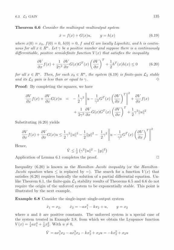
6.3. L2 GAIN 135
Theorem 6.6 Consider the multiinput–multioutput system
x = f(x) + G(x)u, y = h(x) (6.19)
where x(0) = x0, f(0) = 0, h(0) = 0, f and G are locally Lipschitz, and h is contin-uous for all x ∈ Rn. Let γ be a positive number and suppose there is a continuouslydifferentiable, positive semidefinite function V (x) that satisfies the inequality
∂V
∂xf(x) +
12γ2
∂V
∂xG(x)GT (x)
(∂V
∂x
)T
+12hT (x)h(x) ≤ 0 (6.20)
for all x ∈ Rn. Then, for each x0 ∈ Rn, the system (6.19) is finite-gain L2 stableand its L2 gain is less than or equal to γ. �
Proof: By completing the squares, we have
∂V
∂xf(x) +
∂V
∂xG(x)u = − 1
2γ2
∥∥∥∥∥u − 1γ2
GT (x)(
∂V
∂x
)T∥∥∥∥∥
2
+∂V
∂xf(x)
+1
2γ2
∂V
∂xG(x)GT (x)
(∂V
∂x
)T
+12γ2‖u‖2
Substituting (6.20) yields
∂V
∂xf(x) +
∂V
∂xG(x)u ≤ 1
2γ2‖u‖2 − 1
2‖y‖2 − 1
2γ2
∥∥∥∥∥u − 1γ2
GT (x)(
∂V
∂x
)T∥∥∥∥∥
2
Hence,V ≤ 1
2
(γ2‖u‖2 − ‖y‖2
)Application of Lemma 6.1 completes the proof. �
Inequality (6.20) is known as the Hamilton–Jacobi inequality (or the Hamilton–Jacobi equation when ≤ is replaced by =). The search for a function V (x) thatsatisfies (6.20) requires basically the solution of a partial differential equation. Un-like Theorem 6.1, the finite-gain L2 stability results of Theorems 6.5 and 6.6 do notrequire the origin of the unforced system to be exponentially stable. This point isillustrated by the next example.
Example 6.8 Consider the single-input–single-output system
x1 = x2, x2 = −ax31 − kx2 + u, y = x2
where a and k are positive constants. The unforced system is a special case ofthe system treated in Example 3.8, from which we obtain the Lyapunov functionV (x) = 1
4ax41 + 1
2x22. With u �= 0,
V = ax31x2 − ax3
1x2 − kx22 + x2u = −kx2
2 + x2u

136 CHAPTER 6. INPUT-OUTPUT STABILITY
Henceyu = V + ky2
and it follows from Theorem 6.5 that the system is finite-gain L2 stable and itsL2 gain is less than or equal to 1/k. The same conclusion can be arrived at byapplication of Theorem 6.6 after verifying that V (x) = (1/k)(1
4ax41 + 1
2x22) satisfies
the Hamilton–Jacobi inequality (6.20) with γ = 1/k. We note that the conditionsof Theorem 6.1 are not satisfied in this example because the origin of the unforcedsystem is not exponentially stable. Linearization at the origin yields the matrix[
0 10 −k
]
which is not Hurwitz. �
Example 6.9 Consider the linear system
x = Ax + Bu, y = Cx
Suppose P ≥ 0 is a solution of the Riccati equation
PA + AT P +1γ2
PBBT P + CT C = 0 (6.21)
for some γ > 0. Taking V (x) = 12xT Px and using the expression [∂V/∂x] = xT P ,
it can be easily seen that V (x) satisfies the Hamilton–Jacobi equation
xT PAx +1
2γ2xT PBT BPx +
12xT CT Cx = 0
Hence, the system is finite-gain L2 stable and its L2 gain is ≤ γ. �
In Lemma 6.1, we assumed that inequality (6.15) holds globally. It is clear fromthe proof that if the inequality holds only for x ∈ D ⊂ Rn and u ∈ Du ⊂ Rm,where D and Du are domains that contain x = 0 and u = 0, respectively, we willstill arrive at inequality (6.16) as long as x(t) and u(t) stay in D and Du for allt ≥ 0. Ensuring that x(t) remains in some neighborhood of the origin, when both‖x0‖ and sup0≤t≤τ‖u(t)‖ are sufficiently small, follows from asymptotic stability ofthe origin of x = f(x, 0). This fact is used to show small-signal L2 stability in thenext lemma.
Lemma 6.2 Suppose the assumptions of Lemma 6.1 are satisfied for x ∈ D ⊂ Rn
and u ∈ Du ⊂ Rm, where D and Du are domains that contain x = 0 and u = 0,respectively. Suppose further that x = 0 is an asymptotically stable equilibrium pointof x = f(x, 0). Then, there is r > 0 such that for each x0 with ‖x0‖ ≤ r, the system(6.14) is small-signal finite-gain L2 stable with L2 gain less than or equal to γ. �

6.4. EXERCISES 137
Proof: From Lemma 4.7, the system x = f(x, u) is locally input-to-state-stable.Hence, there exist positive constants k1 and k2, a class KL function β, and a classK function γ0 such that for any initial state x0 with ‖x0‖ ≤ k1 and any input u(t)with sup0≤t≤τ ‖u(t)‖ ≤ k2, the solution x(t) satisfies
‖x(t)‖ ≤ max{
β(‖x0‖, t), γ0
(sup
0≤σ≤t‖u(σ)‖
)}for all 0 ≤ t ≤ τ . Thus, by choosing k1 and k2 small enough, we can be sure thatx(t) ∈ D and u(t) ∈ Du for all 0 ≤ t ≤ τ . Proceeding as in the proof of Lemma 6.1we arrive at (6.16). �
With the help of Lemma 6.2, we can state small-signal versions of Theorems 6.5and 6.6.
Theorem 6.7 Consider the system (6.17). Assume (6.18) is satisfied in someneighborhood of (x = 0, u = 0) and the origin is an asymptotically stable equi-librium point of x = f(x, 0). Then, the system is small-signal finite-gain L2 stableand its L2 gain is less than or equal to 1/δ. �
Theorem 6.8 Consider the system (6.19). Assume (6.20) is satisfied in someneighborhood of (x = 0, u = 0) and the origin is an asymptotically stable equi-librium point of x = f(x). Then, the system is small-signal finite-gain L2 stableand its L2 gain is less than or equal to γ. �
Example 6.10 As a variation on the theme of Example 6.8, consider the system
x1 = x2, x2 = −a(x1 − 13x3
1) − kx2 + u, y = x2
where a, k > 0. The function V (x) = a(
12x2
1 − 112x4
1
)+ 1
2x22 is positive semidefinite
in the set {|x1| ≤√
6} and satisfies inequality (6.18) since
V = −kx22 + x2u = −ky2 + yu
With u = 0, V = −kx22 ≤ 0 and asymptotic stability of the origin can be shown by
LaSalle’s invariance principle since
x2(t) ≡ 0 ⇒ x1(t)[3 − x21(t)] ≡ 0 ⇒ x1(t) ≡ 0
in the domain {|x1| <√
3}. Alternatively, we can show asymptotic stability bylinearization, which results in a Hurwitz matrix. By Theorem 6.7, we conclude thatthe system is small-signal finite-gain L2 stable and its L2 gain is ≤ 1/k. �
6.4 Exercises
6.1 Show that the series connection of two L stable (respectively, finite-gain Lstable) systems is L stable (respectively, finite-gain L stable).
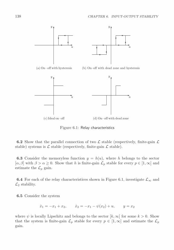
138 CHAPTER 6. INPUT-OUTPUT STABILITY
(a) On–off with hysteresis
(c) Ideal on–off (d) On–off with dead zone
(b) On–off with dead zone and hysteresis
u u
u u
y
y
y
y
Figure 6.1: Relay characteristics
6.2 Show that the parallel connection of two L stable (respectively, finite-gain Lstable) systems is L stable (respectively, finite-gain L stable).
6.3 Consider the memoryless function y = h(u), where h belongs to the sector[α, β] with β > α ≥ 0. Show that h is finite-gain Lp stable for every p ∈ [1,∞] andestimate the Lp gain.
6.4 For each of the relay characteristices shown in Figure 6.1, investigate L∞ andL2 stability.
6.5 Consider the system
x1 = −x1 + x2, x2 = −x1 − ψ(x2) + u, y = x2
where ψ is locally Lipschitz and belongs to the sector [k,∞] for some k > 0. Showthat the system is finite-gain Lp stable for every p ∈ [1,∞] and estimate the Lp
gain.

6.4. EXERCISES 139
6.6 Consider the system
x1 = −x1 + x2, x2 = −ψ(x1) − x2 + u, y = x2
where ψ is locally Lipschitz and belongs to the sector [k,∞] for some k > 0. Showthat the system is L∞ stable. Under what additional conditions on ψ will it befinite-gain L∞ stable?
6.7 For each of the systems in Exercise 4.14, investigate L∞ and finite-gain L∞stability when the output is defined as follows.
(1) y = x (2) y = sin x (3) y = x (4) y = x(5) y = x2
1 (6) y = x1 + x2 (7) y = x1 + x2 (8) y = x2
(9) y = x2 (10) y = x1
6.8 For each of the systems in Exercise 4.15, investigate L∞ and small-signal L∞stability when the output is x1.
6.9 Investigate finite-gain L2 stability of the systems in the following exercises:
(1) Exercise 5.2
(2) Exercise 5.5
(3) Exercise 5.6
When it is stable, estimate the L2 gain.
6.10 Consider the tunnel-diode circuit (A.7) with output y = x2.
(a) Show that the system is L∞ stable.
(b) Show that it is finite-gain L2 stable and estimate the L2 gain.
6.11 Consider the system
x1 = −2x1 + x2, x2 = −2x1 − ψ(x1) + u, y = −x1 + x2
where ψ is a locally Lipschitz passive function.
(a) With u = 0, use V (x) =∫ x1
0ψ(σ)dσ + 1
2x21 + 1
2 (x2 − x1)2 to show that theorigin is globally asymptotically stable.
(b) Show that the system is L∞ stable.
(c) Show that it is finite-gain L2 stable and estimate the L2 gain.
6.12 Show that the system of Exercise 5.5 is finite-gain L2 stable and estimatethe L2 gain.
140 CHAPTER 6. INPUT-OUTPUT STABILITY
6.13 Consider the pendulum equation (A.2) with b > 0.
(a) Show that whether the output is taken as y = x1 or y = x2, the system will besmall-signal finite-gain Lp stable for every p ∈ [1,∞].
(b) If the output is y = x2, show that the system will be finite-gain L2 stable andestimate the L2 gain.
6.14 An m-link robot manipulator is represented by equation (A.35). Supposeg(q) = 0 has an isolated solution q = q∗ and the potential energy P (q) has aminimum at q∗; that is, P (q) ≥ P (q∗) for all q. Let u = −Kdq + v, where Kd is apositive definite symmetric matrix. Show that the system, with input v and outputq is finite-gain L2 stable and estimate the L2 gain. Hint: See Exercise 5.8.
6.15 Consider the system
x1 = −x1 − x2 + u, x2 = ψ1(x1) − ψ2(x2), y = x1
where ψ1 and ψ2 are locally Lipschitz functions and ψi belongs to the sector [αi, βi]with βi > αi > 0.
(a) Show that the system is finite-gain Lp stable for every p ∈ [1,∞] and estimatethe Lp gain.
(b) Apply Theorem 6.6 to show that the L2 gain is ≤ β1/α1.
6.16 Consider the system
x1 = x2, x2 = −ψ(x1) − x2 + u, y = x1 + 2x2
where ψ is locally Lipschitz, ψ(0) = 0, and x1ψ(x1) ≥ αx21 ∀ x1 with α > 0. Apply
Theorem 6.6 to show that the system is finite-gain L2 stable and estimate the L2
gain. Hint: Use a function of the form V (x) = k(xT Px +∫ x1
0ψ(σ) dσ).
6.17 Consider the TORA system (A.49)–(A.52) and let u = −βx2 + w, whereβ > 0. In this exercise we study the L2 stability of the system with input w andoutput x2. Let E(x) be the sum of the potential energy 1
2kx23 and the kinetic energy
12vT Dv, where
v =[x2
x4
]and D =
[J + mL2 mL cos x1
mL cos x1 m + M
]
(a) Using V (x) = αE(x), show that α can be chosen such that V (x) satisfies (6.20).
(b) Show that the system is finite-gain L2 stable and the L2 gain is ≤ 1/β.

Chapter 7
Stability of Feedback Systems
Many systems can be represented by the negative feedback connection of Figure 7.1.This feedback structure brings in new challenges and opportunities. The challengeis exemplified by the fact that the feedback connection of two stable systems couldbe unstable. In the face of this challenge comes the opportunity to take advantageof the feedback structure itself to come up with conditions that guard against insta-bility. For linear time-invariant systems, where H1 and H2 are transfer functions,we know from the Nyquist criterion that the feedback loop will be stable if theloop phase is less than 180 degrees or the loop gain is less than one. The passivitytheorems of Section 7.1 and the small-gain theorem of Section 7.3 extend these twoconditions, respectively, to nonlinear systems.
The main passivity theorem states that the feedback connection of two passivesystems is passive. Under additional conditions, we can show that the feedbackconnection has an asymptotically stable equilibrium point at the origin, or that theinput-output map is finite-gain L2 stable. The connection between passivity andthe phase of a transfer function comes from the frequency-domain characterizationof positive real transfer functions, given in Section 5.3, which shows that the phase
u1 e1 y1
y2 e2 u2
H1
H2
−+
++
Figure 7.1: Feedback connection.
141
142 CHAPTER 7. STABILITY OF FEEDBACK SYSTEMS
of a positive real transfer function cannot exceed 90 degrees. Hence, the loop phasecannot exceed 180 degrees. If one of the two transfer functions is strictly positivereal, the loop phase will be strictly less than 180 degrees. The small-gain theoremdeals with a feedback connection where each component is finite-gain L-stable andrequires the loop gain to be less than one.1
Another opportunity that arises in feedback systems is the possibility of mod-eling the system in such a way that the component in the forward path is a lineartime-invariant system while the one in the feedback path is a memoryless nonlin-earity. The absolute stability results of Section 7.3 take advantage of this structureand provide the circle and Popov criteria, which allow for unknown nonlinearitiesthat belong to a given sector and require frequency-domain conditions on the linearsystem that build on the classical Nyquist criterion and Nyquist plot.
7.1 Passivity Theorems
Consider the feedback connection of Figure 7.1 where each of the feedback compo-nents H1 and H2 is either a time-invariant dynamical system represented by thestate model
xi = fi(xi, ei), yi = hi(xi, ei) (7.1)
or a (possibly time-varying) memoryless function represented by
yi = hi(t, ei) (7.2)
We are interested in using passivity properties of the feedback components H1
and H2 to analyze stability of the feedback connection. We require the feedbackconnection to have a well-defined state model. When both components H1 and H2
are dynamical systems, the closed-loop state model takes the form
x = f(x, u), y = h(x, u) (7.3)
where x = col(x1, x2), u = col(u1, u2), and y = col(y1, y2). We assume that f islocally Lipschitz, h is continuous, f(0, 0) = 0, and h(0, 0) = 0. It can be easilyverified that the feedback connection will have a well-defined state model if theequations
e1 = u1 − h2(x2, e2), e2 = u2 + h1(x1, e1) (7.4)
have a unique solution (e1, e2) for every (x1, x2, u1, u2). The properties f(0, 0) = 0and h(0, 0) = 0 follow from fi(0, 0) = 0 and hi(0, 0) = 0. It is also easy to seethat (7.4) will always have a unique solution if h1 is independent of e1 or h2 isindependent of e2. In this case, the functions f and h of the closed-loop statemodel inherit smoothness properties of the functions fi and hi of the feedbackcomponents. In particular, if fi and hi are locally Lipschitz, so are f and h. For
1Nonlinear extensions of this classical small-gain theorem can be found in [69, 90, 138].
7.1. PASSIVITY THEOREMS 143
linear systems, requiring hi to be independent of ei is equivalent to requiring thetransfer function of Hi to be strictly proper.
When one component, H1 say, is a dynamical system, while the other one is amemoryless function, the closed-loop state model takes the form
x = f(t, x, u), y = h(t, x, u) (7.5)
where x = x1, u = col(u1, u2), and y = col(y1, y2). We assume that f is piecewisecontinuous in t and locally Lipschitz in (x, u), h is piecewise continuous in t andcontinuous in (x, u), f(t, 0, 0) = 0, and h(t, 0, 0) = 0. The feedback connection willhave a well-defined state model if the equations
e1 = u1 − h2(t, e2), e2 = u2 + h1(x1, e1) (7.6)
have a unique solution (e1, e2) for every (x1, t, u1, u2). This will be always the casewhen h1 is independent of e1.
The starting point of our analysis is the following fundamental property:
Theorem 7.1 The feedback connection of two passive systems is passive.
Proof: Let V1(x1) and V2(x2) be the storage functions for H1 and H2, respectively.If either component is a memoryless function, take Vi = 0. Then, eT
i yi ≥ Vi. Fromthe feedback connection of Figure 7.1, we see that
eT1 y1 + eT
2 y2 = (u1 − y2)T y1 + (u2 + y1)T y2 = uT1 y1 + uT
2 y2
Hence,uT y = uT
1 y1 + uT2 y2 ≥ V1 + V2
With V (x) = V1(x1) + V2(x2) as the storage function for the feedback connection,we obtain uT y ≥ V . �
Now we want to use passivity to study stability and asymptotic stability of theorigin of the closed-loop system when the input u = 0. Stability of the origin fol-lows trivially from Theorem 7.1 and Lemma 5.5. Therefore, we focus our attentionon studying asymptotic stability. The next theorem is an immediate consequenceof Theorem 7.1 and Lemma 5.6.
Theorem 7.2 Consider the feedback connection of two time-invariant dynamicalsystems of the form (7.1). The origin of the closed-loop system (7.3) (when u = 0)is asymptotically stable if one of the following conditions is satisfied:
• both feedback components are strictly passive;
• both feedback components are output strictly passive and zero-state observable;
• one component is strictly passive and the other one is output strictly passiveand zero-state observable.
144 CHAPTER 7. STABILITY OF FEEDBACK SYSTEMS
Furthermore, if the storage function for each component is radially unbounded, theorigin is globally asymptotically stable. �
Proof: Let V1(x1) and V2(x2) be the storage functions for H1 and H2, respectively.As in the proof of Lemma 5.6, we can show that V1(x1) and V2(x2) are positivedefinite functions. Take V (x) = V1(x1) + V2(x2) as a Lyapunov function candidatefor the closed-loop system. In the first case, the derivative V satisfies
V ≤ uT y − ψ1(x1) − ψ2(x2) = −ψ1(x1) − ψ2(x2)
since u = 0. Hence, the origin is asymptotically stable. In the second case,
V ≤ −yT1 ρ1(y1) − yT
2 ρ2(y2)
where yTi ρi(yi) > 0 for all yi �= 0. Here V is only negative semidefinite and V = 0 ⇒
y = 0. To apply the invariance principle, we need to show that y(t) ≡ 0 ⇒ x(t) ≡ 0.Note that y2(t) ≡ 0 ⇒ e1(t) ≡ 0. By zero-state observability of H1, y1(t) ≡ 0 ⇒x1(t) ≡ 0. Similarly, y1(t) ≡ 0 ⇒ e2(t) ≡ 0 and, by zero-state observability of H2,y2(t) ≡ 0 ⇒ x2(t) ≡ 0. Thus, the origin is asymptotically stable. In the third case(with H1 as the strictly passive component),
V ≤ −ψ1(x1) − yT2 ρ2(y2)
and V = 0 implies x1 = 0 and y2 = 0. Once again, y2(t) ≡ 0 ⇒ e1(t) ≡ 0, whichtogether with x1(t) ≡ 0 imply that y1(t) ≡ 0. Hence, e2(t) ≡ 0 and, by zero-stateobservability of H2, y2(t) ≡ 0 ⇒ x2(t) ≡ 0. Thus, the origin is asymptoticallystable. Finally, if V1(x1) and V2(x2) are radially unbounded, so is V (x), and we canconclude global asymptotic stability. �
The proof uses the sum of the storage functions for the feedback components as aLyapunov function candidate for the feedback connection. The analysis is restrictivebecause, to show that V = V1 + V2 ≤ 0, we insist that both V1 ≤ 0 and V2 ≤ 0.Clearly, this is not necessary. One term, V1 say, could be positive over some regionas long as the sum V ≤ 0 over the same region. This idea is exploited in Examples7.2 and 7.3, while Example 7.1 is a straightforward application of Theorem 7.2.
Example 7.1 Consider the feedback connection of
H1 :
⎧⎨⎩
x1 = x2
x2 = −ax31 − kx2 + e1
y1 = x2
and H2 :
⎧⎨⎩
x3 = x4
x4 = −bx3 − x34 + e2
y2 = x4
where a, b, and k are positive constants. Using V1 = 14ax4
1 + 12x2
2 as a storagefunction for H1, we obtain
V1 = ax31x2 − ax3
1x2 − kx22 + x2e1 = −ky2
1 + y1e1
7.1. PASSIVITY THEOREMS 145
Hence, H1 is output strictly passive. Besides, with e1 = 0, we have
y1(t) ≡ 0 ⇔ x2(t) ≡ 0 ⇒ x1(t) ≡ 0
which shows that H1 is zero-state observable. Using V2 = 12bx2
3 + 12x2
4 as a storagefunction for H2, we obtain
V2 = bx3x4 − bx3x4 − x44 + x4e2 = −y4
2 + y2e2
Therefore, H2 is output strictly passive. Moreover, with e2 = 0, we have
y2(t) ≡ 0 ⇔ x4(t) ≡ 0 ⇒ x3(t) ≡ 0
which shows that H2 is zero-state observable. Thus, by the second case of Theo-rem 7.2 and the fact that V1 and V2 are radially unbounded, we conclude that theorigin is globally asymptotically stable. �Example 7.2 Reconsider the feedback connection of the previous example, butchange the output of H1 to y1 = x2 + e1. From the expression
V1 = −kx22 + x2e1 = −k(y1 − e1)2 − e2
1 + y1e1
we can conclude that H1 is passive, but we cannot conclude strict passivity oroutput strict passivity. Therefore, we cannot apply Theorem 7.2. Using
V = V1 + V2 = 14ax4
1 + 12x2
2 + 12bx2
3 + 12x2
4
as a Lyapunov function candidate for the closed-loop system, we obtain
V = −kx22 + x2e1 − x4
4 + x4e2 = −kx22 − x2x4 − x4
4 + x4(x2 − x4)= −kx2
2 − x44 − x2
4 ≤ 0
Moreover, V = 0 implies that x2 = x4 = 0 and
x2(t) ≡ 0 ⇒ ax31(t) − x4(t) ≡ 0 ⇒ x1(t) ≡ 0
x4(t) ≡ 0 ⇒ −bx3(t) + x2(t) − x4(t) ≡ 0 ⇒ x3(t) ≡ 0
Thus, by the invariance principle and the fact that V is radially unbounded, weconclude that the origin is globally asymptotically stable. �Example 7.3 Reconsider the system
x1 = x2, x2 = −h1(x1) − h2(x2)
from Examples 3.8 and 3.9, where h1 and h2 are locally Lipschitz and belong tothe sector (0,∞). The system can be viewed as the state model of the feedbackconnection of Figure 7.2, where H1 consists of a negative feedback loop around the
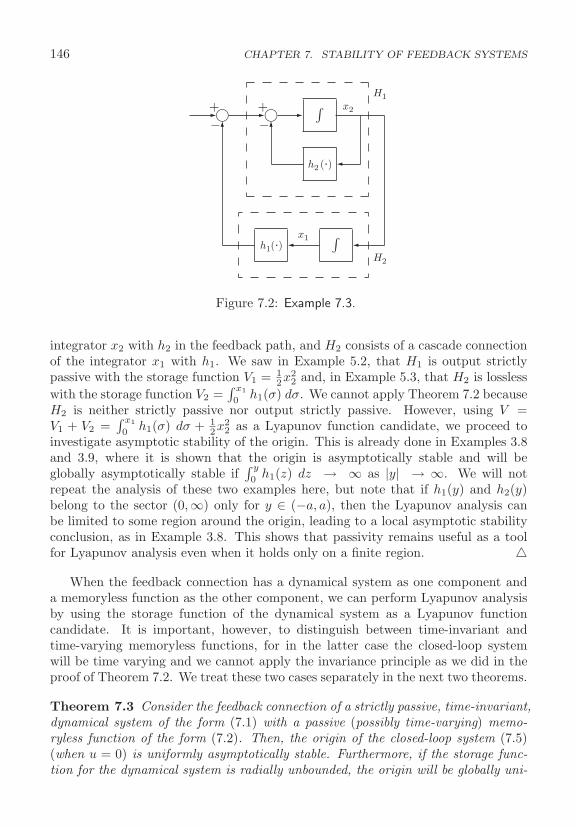
146 CHAPTER 7. STABILITY OF FEEDBACK SYSTEMS
+−
+−
H1
H2
x2
x1
h2 (.)
h1(.)
Figure 7.2: Example 7.3.
integrator x2 with h2 in the feedback path, and H2 consists of a cascade connectionof the integrator x1 with h1. We saw in Example 5.2, that H1 is output strictlypassive with the storage function V1 = 1
2x22 and, in Example 5.3, that H2 is lossless
with the storage function V2 =∫ x1
0h1(σ) dσ. We cannot apply Theorem 7.2 because
H2 is neither strictly passive nor output strictly passive. However, using V =V1 + V2 =
∫ x1
0h1(σ) dσ + 1
2x22 as a Lyapunov function candidate, we proceed to
investigate asymptotic stability of the origin. This is already done in Examples 3.8and 3.9, where it is shown that the origin is asymptotically stable and will beglobally asymptotically stable if
∫ y
0h1(z) dz → ∞ as |y| → ∞. We will not
repeat the analysis of these two examples here, but note that if h1(y) and h2(y)belong to the sector (0,∞) only for y ∈ (−a, a), then the Lyapunov analysis canbe limited to some region around the origin, leading to a local asymptotic stabilityconclusion, as in Example 3.8. This shows that passivity remains useful as a toolfor Lyapunov analysis even when it holds only on a finite region. �
When the feedback connection has a dynamical system as one component anda memoryless function as the other component, we can perform Lyapunov analysisby using the storage function of the dynamical system as a Lyapunov functioncandidate. It is important, however, to distinguish between time-invariant andtime-varying memoryless functions, for in the latter case the closed-loop systemwill be time varying and we cannot apply the invariance principle as we did in theproof of Theorem 7.2. We treat these two cases separately in the next two theorems.
Theorem 7.3 Consider the feedback connection of a strictly passive, time-invariant,dynamical system of the form (7.1) with a passive (possibly time-varying) memo-ryless function of the form (7.2). Then, the origin of the closed-loop system (7.5)(when u = 0) is uniformly asymptotically stable. Furthermore, if the storage func-tion for the dynamical system is radially unbounded, the origin will be globally uni-

7.1. PASSIVITY THEOREMS 147
formly asymptotically stable. �
Proof: As in the proof of Lemma 5.6, it can be shown that V1(x1) is positivedefinite. Its derivative is given by
V1 =∂V1
∂x1f1(x1, e1) ≤ eT
1 y1 − ψ1(x1) = −eT2 y2 − ψ1(x1) ≤ −ψ1(x1)
The conclusion follows from Theorem 4.2. �
Theorem 7.4 Consider the feedback connection of a time-invariant dynamical sys-tem H1 of the form (7.1) with a time-invariant memoryless function H2 of the form(7.2). Suppose that H1 is zero-state observable and has a positive definite storagefunction V1(x), which satisfies
eT1 y1 ≥ V1 + yT
1 ρ1(y1) (7.7)
and that H2 satisfieseT2 y2 ≥ eT
2 ϕ2(e2) (7.8)
Then, the origin of the closed-loop system (7.5) (when u = 0) is asymptoticallystable if
vT [ρ1(v) + ϕ2(v)] > 0, ∀ v �= 0 (7.9)
Furthermore, if V1 is radially unbounded, the origin will be globally asymptoticallystable. �
Proof: Use V1(x1) as a Lyapunov function candidate, to obtain
V1 =∂V1
∂x1f1(x1, e1) ≤ eT
1 y1 − yT1 ρ1(y1)
= −eT2 y2 − yT
1 ρ1(y1) ≤ −[yT1 ϕ2(y1) + yT
1 ρ1(y1)]
Inequality (7.9) shows that V1 ≤ 0 and V1 = 0 ⇒ y1 = 0. Noting that y1(t) ≡0 ⇒ e2(t) ≡ 0 ⇒ e1(t) ≡ 0, we see that zero-state observability of H1 implies thatx1(t) ≡ 0. The conclusion follows from the invariance principle. �
Example 7.4 Consider the feedback connection of a strictly positive real transferfunction and a passive time-varying memoryless function. From Lemma 5.4, weknow that the dynamical system is strictly passive with a positive definite storagefunction of the form V (x) = 1
2xT Px. From Theorem 7.3, we conclude that theorigin of the closed-loop system is globally uniformly asymptotically stable. This isa version of the circle criterion of Section 7.3. �Example 7.5 Consider the feedback connection of
H1 :{
x = f(x) + G(x)e1
y1 = h(x) and H2 : y2 = σ(e2)

148 CHAPTER 7. STABILITY OF FEEDBACK SYSTEMS
where ei, yi ∈ Rm, σ(0) = 0, and eT2 σ(e2) > 0 for all e2 �= 0. Suppose there is a
radially unbounded positive definite function V1(x) such that
∂V1
∂xf(x) ≤ 0,
∂V1
∂xG(x) = hT (x), ∀ x ∈ Rn
and H1 is zero-state observable. Both components are passive. Moreover, H2
satisfies eT2 y2 = eT
2 σ(e2). Thus, (7.7) is satisfied with ρ1 = 0, and (7.8) is satisfiedwith ϕ2 = σ. Since vσ(v) > 0 for all v �= 0, (7.9) is satisfied. It follows fromTheorem 7.4 that the origin of the closed-loop system is globally asymptoticallystable. �
The utility of Theorems 7.3 and 7.4 can be extended by loop transformations.Suppose H1 is a time-invariant dynamical system, while H2 is a (possibly time-varying) memoryless function that belongs to the sector [K1,K2], where K = K2 −K1 is a positive definite symmetric matrix. We saw in Section 5.1 that a function inthe sector [K1,K2] can be transformed into a function in the sector [0,∞] by inputfeedforward followed by output feedback, as shown in Figure 5.5. Input feedforwardon H2 can be nullified by output feedback on H1, as shown in Figure 7.3(b), resultingin an equivalent feedback connection, as far as asymptotic stability of the originis concerned. Similarly, premultiplying the modified H2 by K−1 can be nullifiedby postmultiplying the modified H1 by K, as shown in Figure 7.3(c). Finally,output feedback on the component in the feedback path can be nullified by inputfeedforward on the component in the forward path, as shown in Figure 7.3(d).The reconfigured feedback connection has two components H1 and H2, where H2
is a memoryless function that belongs to the sector [0,∞]. We can now applyTheorem 7.3 if H2 is time varying or Theorem 7.4 if it is time invariant.
Example 7.6 Consider the feedback connection of
H1 :
⎧⎨⎩
x1 = x2
x2 = −h(x1) + cx2 + e1
y1 = x2
and H2 : y2 = σ(e2)
where σ ∈ [α, β], h ∈ [α1,∞], c > 0, α1 > 0, and b = β − α > 0. Applying the looptransformation of Figure 7.3(d) (with K1 = α and K2 = β) results in the feedbackconnection of
H1 :
⎧⎨⎩
x1 = x2
x2 = −h(x1) − ax2 + e1
y1 = bx2 + e1
and H2 : y2 = σ(e2)
where σ ∈ [0,∞] and a = α− c. When α > c, it is shown in Example 5.4 that H1 isstrictly passive with a radially unbounded storage function. Thus, we conclude fromTheorem 7.3 that the origin of the feedback connection is globally asymptoticallystable. �
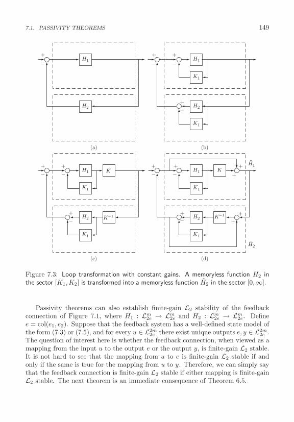
7.1. PASSIVITY THEOREMS 149
+
−+
−+
−
+
−
K+
−+
−
+−
K
K−1 K−1
H2
H1+
−+
−
++
+
+
+−
H1 H1
H2 H2
H1 H1
H2 H2
K1
K1
K1K1
K1K1
(a) (b)
(c) (d)
Figure 7.3: Loop transformation with constant gains. A memoryless function H2 inthe sector [K1,K2] is transformed into a memoryless function H2 in the sector [0,∞].
Passivity theorems can also establish finite-gain L2 stability of the feedbackconnection of Figure 7.1, where H1 : Lm
2e → Lm2e and H2 : Lm
2e → Lm2e. Define
e = col(e1, e2). Suppose that the feedback system has a well-defined state model ofthe form (7.3) or (7.5), and for every u ∈ L2m
2e there exist unique outputs e, y ∈ L2m2e .
The question of interest here is whether the feedback connection, when viewed as amapping from the input u to the output e or the output y, is finite-gain L2 stable.It is not hard to see that the mapping from u to e is finite-gain L2 stable if andonly if the same is true for the mapping from u to y. Therefore, we can simply saythat the feedback connection is finite-gain L2 stable if either mapping is finite-gainL2 stable. The next theorem is an immediate consequence of Theorem 6.5.
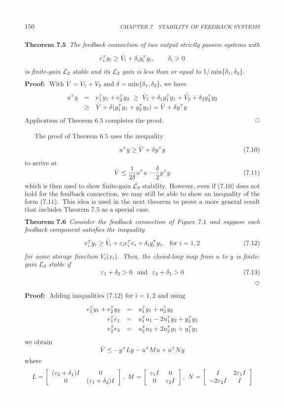
150 CHAPTER 7. STABILITY OF FEEDBACK SYSTEMS
Theorem 7.5 The feedback connection of two output strictly passive systems with
eT
i yi ≥ Vi + δiyT
i yi, δi > 0
is finite-gain L2 stable and its L2 gain is less than or equal to 1/min{δ1, δ2}.Proof: With V = V1 + V2 and δ = min{δ1, δ2}, we have
uT y = eT
1 y1 + eT
2 y2 ≥ V1 + δ1yT
1 y1 + V2 + δ2yT
2 y2
≥ V + δ(yT
1 y1 + yT
2 y2) = V + δyT y
Application of Theorem 6.5 completes the proof. �
The proof of Theorem 6.5 uses the inequality
uT y ≥ V + δyT y (7.10)
to arrive atV ≤ 1
2δuT u − δ
2yT y (7.11)
which is then used to show finite-gain L2 stability. However, even if (7.10) does nothold for the feedback connection, we may still be able to show an inequality of theform (7.11). This idea is used in the next theorem to prove a more general resultthat includes Theorem 7.5 as a special case.
Theorem 7.6 Consider the feedback connection of Figure 7.1 and suppose eachfeedback component satisfies the inequality
eT
i yi ≥ Vi + εieT
i ei + δiyT
i yi, for i = 1, 2 (7.12)
for some storage function Vi(xi). Then, the closed-loop map from u to y is finite-gain L2 stable if
ε1 + δ2 > 0 and ε2 + δ1 > 0 (7.13)
�
Proof: Adding inequalities (7.12) for i = 1, 2 and using
eT
1 y1 + eT
2 y2 = uT
1 y1 + uT
2 y2
eT
1 e1 = uT
1 u1 − 2uT
1 y2 + yT
2 y2
eT
2 e2 = uT
2 u2 + 2uT
2 y1 + yT
1 y1
we obtainV ≤ −yT Ly − uT Mu + uT Ny
where
L =[
(ε2 + δ1)I 00 (ε1 + δ2)I
], M =
[ε1I 00 ε2I
], N =
[I 2ε1I
−2ε2I I
]

7.1. PASSIVITY THEOREMS 151
and V (x) = V1(x1) + V2(x2). Let a = min{ε2 + δ1, ε1 + δ2} > 0, b = ‖N‖ ≥ 0, andc = ‖M‖ ≥ 0. Then
V ≤ −a‖y‖2 + b‖u‖‖y‖ + c‖u‖2
= − 12a
(b‖u‖ − a‖y‖)2 +b2
2a‖u‖2 − a
2‖y‖2 + c‖u‖2
≤ k2
2a‖u‖2 − a
2‖y‖2
where k2 = b2 + 2ac. Application of Lemma 6.1 completes the proof. �
Theorem 7.6 reduces to Theorem 7.5 when (7.12) is satisfied with ε1 = ε2 = 0,δ1 > 0, and δ2 > 0. However, condition (7.13) is satisfied in several other cases.For example, it is satisfied when both H1 and H2 are input strictly passive witheT
i yi ≥ Vi +εiuTi ui for some εi > 0. It is also satisfied when one component (H1, for
example) is passive, while the other component satisfies (7.12) with positive ε2 andδ2. What is more interesting is that (7.13) can be satisfied even when some of theconstants εi and δi are negative. For example, a negative ε1 can be compensatedfor by a positive δ2 and vice versa.
Example 7.7 Consider the feedback connection of
H1 :{
x = f(x) + G(x)e1
y1 = h(x) and H2 : y2 = σ(e2)
where ei, yi ∈ Rm and σ is a decoupled nonlinearity as in (5.1) with each componentσk in the sector [α, β] with β > α > 0. Suppose there is a positive semidefinitefunction V1(x) such that
∂V1
∂xf(x) ≤ 0,
∂V1
∂xG(x) = hT (x), ∀ x ∈ Rn
Both components are passive. Moreover, H2 satisfies
αeT
2 e2 ≤ eT
2 y2 ≤ βeT
2 e2 and1β
yT
2 y2 ≤ eT
2 y2 ≤ 1α
yT
2 y2
Hence,
eT
2 y2 = γeT
2 y2 + (1 − γ)eT
2 y2 ≥ γαeT
2 e2 + (1 − γ)1β
yT
2 y2, 0 < γ < 1
Thus, (7.9) is satisfied with ε1 = δ1 = 0, ε2 = γα, and δ2 = (1 − γ)/β. This showsthat (7.13) is satisfied, and we conclude that the closed-loop map from u to y isfinite-gain L2 stable. �
152 CHAPTER 7. STABILITY OF FEEDBACK SYSTEMS
Example 7.8 Consider the feedback connection of
H1 :
⎧⎨⎩
x1 = x2
x2 = −ax31 − σ(x2) + e1
y1 = x2
and H2 : y2 = ke2
where σ ∈ [−α,∞], a > 0, α > 0, and k > 0. If σ was in the sector [0,∞], we couldhave shown that H1 is passive with the storage function V1(x) = 1
4ax41 + 1
2x22. For
σ ∈ [−α,∞], we have
V1 = ax31x2 − ax3
1x2 − x2σ(x2) + x2e1 ≤ αx22 + x2e1 = αy2
1 + y1e1
Hence, (7.9) is satisfied for H1 with ε1 = 0 and δ1 = −α. Since
e2y2 = ke22 = γke2
2 +(1 − γ)
ky22 , 0 < γ < 1
(7.9) is satisfied for H2 with ε2 = γk and δ2 = (1 − γ)/k. If k > α, we can chooseγ such that γk > α. Then, ε1 + δ2 > 0 and ε2 + δ1 > 0. We conclude that theclosed-loop map from u to y is finite-gain L2 stable if k > α.. �
7.2 The Small-Gain Theorem
Consider the feedback connection of Figure 7.1 where H1 : Lme → Lq
e and H2 : Lqe →
Lme . Suppose both systems are finite-gain L stable; that is,
‖y1τ‖L ≤ γ1‖e1τ‖L + β1, ∀ e1 ∈ Lme , ∀ τ ∈ [0,∞) (7.14)
‖y2τ‖L ≤ γ2‖e2τ‖L + β2, ∀ e2 ∈ Lqe, ∀ τ ∈ [0,∞) (7.15)
Suppose further that the feedback system is well defined in the sense that for everypair of inputs u1 ∈ Lm
e and u2 ∈ Lqe, there exist unique outputs e1, y2 ∈ Lm
e
and e2, y1 ∈ Lqe. If H1 and H2 are represented by state models, we assume that
the feedback connection has a well-defined state model. Define u = col(u1, u2),y = col(y1, y2), and e = col(e1, e2). The next (small-gain) theorem gives a sufficientcondition for the feedback connection to be finite-gain L stable; that is, the mappingfrom u to e, or equivalently from u to y, is finite-gain L stable.
Theorem 7.7 Under the preceding assumptions, the feedback connection is finite-gain L stable if γ1γ2 < 1. �
Proof: Throughout the proof, ‖ · ‖ stands for ‖ · ‖L. Assuming existence of thesolution, we can write
e1τ = u1τ − (H2e2)τ , e2τ = u2τ + (H1e1)τ
7.2. THE SMALL-GAIN THEOREM 153
Then,
‖e1τ‖ ≤ ‖u1τ‖ + ‖(H2e2)τ‖ ≤ ‖u1τ‖ + γ2‖e2τ‖ + β2
≤ ‖u1τ‖ + γ2 (‖u2τ‖ + γ1‖e1τ‖ + β1) + β2
= γ1γ2‖e1τ‖ + (‖u1τ‖ + γ2‖u2τ‖ + β2 + γ2β1)
Since γ1γ2 < 1,
‖e1τ‖ ≤ 11 − γ1γ2
(‖u1τ‖ + γ2‖u2τ‖ + β2 + γ2β1) (7.16)
for all τ ∈ [0,∞). Similarly,
‖e2τ‖ ≤ 11 − γ1γ2
(‖u2τ‖ + γ1‖u1τ‖ + β1 + γ1β2) (7.17)
for all τ ∈ [0,∞). The proof is completed by noting that ‖e‖ ≤ ‖e1‖ + ‖e2‖, whichfollows from the triangle inequality. �
The feedback connection of Figure 7.1 provides a convenient setup for studyingrobustness issues in feedback systems. Quite often, feedback systems subject tomodel uncertainties can be represented in the form of a feedback connection withH1, say, as a stable nominal system and H2 a stable perturbation. Then, therequirement γ1γ2 < 1 is satisfied whenever γ2 is small enough. Therefore, thesmall-gain theorem provides a conceptual framework for understanding many ofthe robustness results that arise in the study of feedback systems.
Example 7.9 Consider the feedback connection of Figure 7.1, with m = q. LetH1 be a linear time-invariant system with a Hurwitz transfer function G(s). LetH2 be a memoryless function y2 = ψ(t, e2) that satisfies
‖ψ(t, y)‖ ≤ γ2‖y‖, ∀ t ≥ 0, ∀ y ∈ Rm
From Theorem 6.4, we know that H1 is finite-gain L2 stable and its L2 gain is≤ γ1 = supw∈R ‖G(jω)‖. It is easy to verify that H2 is finite-gain L2 stable and itsL2 gain is ≤ γ2. Assuming the feedback connection is well defined, we conclude byTheorem 7.7 that it is finite-gain L2 stable if γ1γ2 < 1.2 �Example 7.10 Consider the system3
x = f(t, x, v + d1(t)), εz = Az + B[u + d2(t)], v = Cz
where f is a smooth function of its arguments, A is a Hurwitz matrix, −CA−1B = I,ε is a small positive parameter, and d1, d2 are disturbance signals. The linear
2The same condition results from applying the circle criterion; see Example 7.11.3The example is taken from [139].
154 CHAPTER 7. STABILITY OF FEEDBACK SYSTEMS
part of this model represents actuator dynamics that are, typically, much fasterthan the plant dynamics represented here by the nonlinear equation x = f . Thedisturbance signals d1 and d2 enter the system at the inputs of the plant andactuator, respectively. Suppose the disturbance signals d1 and d2 belong to a signalspace L, where L could be any Lp space, and the goal is to attenuate the effect ofthis disturbance on the state x. This goal can be met if feedback control can bedesigned so that the closed-loop input–output map from (d1, d2) to x is finite-gainL stable and the L gain is less than some given tolerance δ > 0. To simplify thedesign problem, it is common to neglect the actuator dynamics by setting ε = 0and substituting v = −CA−1B(u+d2) = u+d2 in the plant equation to obtain thereduced-order model
x = f(t, x, u + d)
where d = d1+d2. Assuming that the state variables are available for measurement,we use this model to design state feedback control to meet the design objective.Suppose we have designed a smooth state feedback control u = φ(t, x) such that
‖x‖L ≤ γ‖d‖L + β (7.18)
for some γ < δ. Will the control meet the design objective when applied to theactual system with the actuator dynamics included? This is a question of robustnessof the controller with respect to the unmodeled actuator dynamics. When thecontrol is applied to the actual system, the closed-loop equation is given by
x = f(t, x, Cz + d1(t)), εz = Az + B[φ(t, x) + d2(t)]
Let us assume that d2(t) is differentiable and d2 ∈ L. The change of variables
η = z + A−1B[φ(t, x) + d2(t)]
brings the closed-loop system into the form
x = f(t, x, φ(t, x) + d(t) + Cη), εη = Aη + εA−1B[φ + d2(t)]
where
φ =∂φ
∂t+
∂φ
∂xf(t, x, φ(t, x) + d(t) + Cη)
It is not difficult to see that the closed-loop system can be represented in the formof Figure 7.1 with H1 defined by
x = f(t, x, φ(t, x) + e1), y1 = φ =∂φ
∂t+
∂φ
∂xf(t, x, φ(t, x) + e1)
H2 defined by
η =1εAη + A−1Be2, y2 = −Cη
7.3. ABSOLUTE STABILITY 155
u1 = d1 +d2 = d, and u2 = d2. In this representation, the system H1 is the nominalreduced-order closed-loop system, while H2 represents the effect of the unmodeleddynamics. Setting ε = 0 opens the loop and the overall closed-loop system reducesto the nominal one. Let us assume that the feedback function φ(t, x) satisfies theinequality ∥∥∥∥∂φ
∂t+
∂φ
∂xf(t, x, φ(t, x) + e1)
∥∥∥∥ ≤ c1‖x‖ + c2‖e1‖ (7.19)
for all (t, x, e1), where c1 and c2 are nonnegative constants. Using (7.18) and (7.19),it can be shown that
‖y1‖L ≤ γ1‖e1‖L + β1 where γ1 = c1γ + c2, β1 = c1β
Since H2 is a linear time-invariant system and A is Hurwitz, we apply Theorem 6.1with V (η) = εηT Pη, where P is the solution of the Lyapunov equation PA+AT P =−I, to show that H2 is finite-gain Lp stable for every p ∈ [1,∞] and
‖y2‖L ≤ γ2‖e2‖L + β2def= εγf‖e2‖L + β2
where γf = 2λ2max(P )‖A−1B‖‖C‖/λmin(P ). Thus, assuming the feedback connec-
tion is well defined, we conclude from Theorem 7.7 that the input–output map fromu to e is finite-gain L stable if εγfγ1 < 1. From (7.16),
‖e1‖L ≤ 11 − εγ1γf
[‖u1‖L + εγf‖u2‖L + εγfβ1 + β2]
Using‖x‖L ≤ γ‖e1‖L + β
which follows from (7.18), and the definition of u1 and u2, we obtain
‖x‖L ≤ γ
1 − εγ1γf[‖d‖L + εγf‖d2‖L + εγfβ1 + β2] + β (7.20)
The right-hand side of (7.20) approaches γ‖d‖L + β + γβ2 as ε → 0, which showsthat for sufficiently small ε the upper bound on the L gain of the map from d tox, under the actual closed-loop system, will be close to the corresponding quantityunder the nominal closed-loop system. �
7.3 Absolute Stability
Consider the feedback connection of Figure 7.4. We assume that the external inputr = 0 and study the behavior of the unforced system, represented by
x = Ax + Bu, y = Cx + Du, u = −ψ(t, y) (7.21)

156 CHAPTER 7. STABILITY OF FEEDBACK SYSTEMS
r u y
−+
ψ(.)
G(s)
Figure 7.4: Feedback connection.
where x ∈ Rn, u, y ∈ Rm, (A,B) is controllable, (A,C) is observable, and ψ isa memoryless, possibly time-varying, nonlinearity, which is piecewise continuousin t and locally Lipschitz in y. We assume that the feedback connection has awell-defined state model, which is the case when
u = −ψ(t, Cx + Du) (7.22)
has a unique solution u for every (t, x) in the domain of interest. This is always thecase when D = 0. The transfer function matrix of the linear system
G(s) = C(sI − A)−1B + D (7.23)
is square and proper. The controllability and observability assumptions ensure that{A,B,C,D} is a minimal realization of G(s). The nonlinearity ψ is required tosatisfy a sector condition per Definition 5.2. The sector condition may be satisfiedglobally, that is, for all y ∈ Rm, or satisfied only for y ∈ Y , a subset of Rm, whoseinterior is connected and contains the origin.
For all nonlinearities satisfying the sector condition, the origin x = 0 is anequilibrium point of the system (7.21). The problem of interest here is to studythe stability of the origin, not for a given nonlinearity, but rather for a class ofnonlinearities that satisfy a given sector condition. If we succeed in showing thatthe origin is uniformly asymptotically stable for all nonlinearities in the sector, thesystem is said to be absolutely stable. The problem was originally formulated byLure and is sometimes called Lure’s problem.4 Traditionally, absolute stability hasbeen defined for the case when the origin is globally uniformly asymptotically stable.To keep up this tradition, we will use the phrase “absolute stability” when the sectorcondition is satisfied globally and the origin is globally uniformly asymptoticallystable. Otherwise, we will use the phrase “absolute stability with finite domain.”
Definition 7.1 Consider the system (7.21), where ψ satisfies a sector conditionper Definition 5.2. The system is absolutely stable if the origin is globally uniformlyasymptotically stable for any nonlinearity in the given sector. It is absolutely stablewith finite domain if the origin is uniformly asymptotically stable.
4For a historical perspective and further reading, see [63, 96, 97, 125].
7.3. ABSOLUTE STABILITY 157
We will investigate asymptotic stability of the origin by using Lyapunov analy-sis. A Lyapunov function candidate can be chosen by using the passivity tools ofSection 7.1. In particular, if the closed-loop system can be represented as a feed-back connection of two passive systems, then the sum of the two storage functionscan be used as a Lyapunov function candidate for the closed-loop system. The useof loop transformations allows us to cover various sectors and Lyapunov functioncandidates, leading to the circle and Popov criteria.
7.3.1 Circle Criterion
Theorem 7.8 The system (7.21) is absolutely stable if
• ψ ∈ [K1,∞] and G(s)[I + K1G(s)]−1 is strictly positive real, or
• ψ ∈ [K1,K2], with K = K2 −K1 = KT > 0, and [I +K2G(s)][I +K1G(s)]−1
is strictly positive real.
If the sector condition is satisfied only on a set Y ⊂ Rm, then the foregoing condi-tions ensure absolute stability with finite domain. �
We refer to this theorem as the multivariable circle criterion, although the reasonfor using this name will not be clear until we specialize it to the single-input–single-output case. A necessary condition for equation (7.22) to have a unique solution ufor every ψ ∈ [K1,∞] or ψ ∈ [K1,K2] is the nonsingularity of the matrix (I +K1D).This can be seen by taking ψ = K1y in (7.22). Therefore, the transfer function[I + K1G(s)]−1 is proper.
Proof of Theorem 7.8: We prove the theorem first for the sector [0,∞] and re-cover the other cases by loop transformations. If ψ ∈ [0,∞] and G(s) is strictly pos-itive real, we have a feedback connection of two passive systems. From Lemma 5.4,we know that the storage function for the linear dynamical system is V (x) = 1
2xT Px,where P = PT > 0 satisfies the Kalman–Yakubovich–Popov equations (5.13)–(5.15). Using V (x) as a Lyapunov function candidate, we obtain
V = 12xT P x + 1
2 xT Px = 12xT (PA + AT P )x + xT PBu
Using (5.13) and (5.14) yields
V = − 12xT LT Lx − 1
2εxT Px + xT (CT − LT W )u
= − 12xT LT Lx − 1
2εxT Px + (Cx + Du)T u − uT Du − xT LT Wu
Using (5.15) and the fact that uT Du = 12uT (D + DT )u, we obtain
V = − 12εxT Px − 1
2 (Lx + Wu)T (Lx + Wu) − yT ψ(t, y)
Since yT ψ(t, y) ≥ 0, we haveV ≤ − 1
2εxT Px

158 CHAPTER 7. STABILITY OF FEEDBACK SYSTEMS
which shows that the origin is globally exponentially stable. If ψ satisfies the sectorcondition only for y ∈ Y , the foregoing analysis will be valid in some neighborhoodof the origin, showing that the origin is exponentially stable. The case ψ ∈ [K1,∞]can be transformed to a case where the nonlinearity belongs to [0,∞] via the looptransformation of Figure 7.3(b). Hence, the system is absolutely stable if G(s)[I +K1G(s)]−1 is strictly positive real. The case ψ ∈ [K1,K2] can be transformedto a case where the nonlinearity belongs to [0,∞] via the loop transformation ofFigure 7.3(d). Hence, the system is absolutely stable if
I + KG(s)[I + K1G(s)]−1 = [I + K2G(s)][I + K1G(s)]−1
is strictly positive real. �
Example 7.11 Consider the system (7.21) and suppose G(s) is Hurwitz and strictlyproper. Let
γ1 = supω∈R
σmax[G(jω)] = supω∈R
‖G(jω)‖
where σmax[·] denotes the maximum singular value of a complex matrix. The con-stant γ1 is finite since G(s) is Hurwitz. Suppose ψ satisfies the inequality
‖ψ(t, y)‖ ≤ γ2‖y‖, ∀ t ≥ 0, ∀ y ∈ Rm (7.24)
then it belongs to the sector [K1,K2] with K1 = −γ2I and K2 = γ2I. To applyTheorem 7.8, we need to show that
Z(s) = [I + γ2G(s)][I − γ2G(s)]−1
is strictly positive real. We note that det[Z(s) + ZT (−s)] is not identically zerobecause Z(∞) = I. We apply Lemma 5.1. Since G(s) is Hurwitz, Z(s) will beHurwitz if [I − γ2G(s)]−1 is Hurwitz. Noting that5
σmin[I − γ2G(jω)] ≥ 1 − γ1γ2
we see that if γ1γ2 < 1, the plot of det[I−γ2G(jω)] will not go through nor encirclethe origin. Hence, by the multivariable Nyquist criterion,6 [I−γ2G(s)]−1 is Hurwitz;consequently, Z(s) is Hurwitz. Next, we show that Z(jω)+ZT (−jω) > 0, ∀ ω ∈ R.
Z(jω) + ZT (−jω) = [I + γ2G(jω)][I − γ2G(jω)]−1
+ [I − γ2GT (−jω)]−1[I + γ2G
T (−jω)]= [I − γ2G
T (−jω)]−1[2I − 2γ2
2GT (−jω)G(jω)]
× [I − γ2G(jω)]−1
5The following properties of singular values of a complex matrix are used:
det G = 0 ⇔ σmin[G] > 0, σmax[G−1] = 1/σmin[G], if σmin[G] > 0
σmin[I + G] ≥ 1 − σmax[G], σmax[G1G2] ≤ σmax[G1]σmax[G2]
6See [21, pp. 160–161] for a statement of the multivariable Nyquist criterion.
7.3. ABSOLUTE STABILITY 159
Hence, Z(jω) + ZT (−jω) is positive definite for all ω ∈ R if and only if
σmin
[I − γ2
2GT (−jω)G(jω)]
> 0, ∀ ω ∈ R
Now, for γ1γ2 < 1, we have
σmin[I − γ22GT (−jω)G(jω)] ≥ 1 − γ2
2σmax[GT (−jω)]σmax[G(jω)]≥ 1 − γ2
1γ22 > 0
Finally, Z(∞) + ZT (∞) = 2I. Thus, all the conditions of Lemma 5.1 are satisfiedand we conclude that Z(s) is strictly positive real and the system is absolutely stableif γ1γ2 < 1. This is a robustness result, which shows that closing the loop arounda Hurwitz transfer function with a nonlinearity satisfying (7.24), with a sufficientlysmall γ2, does not destroy the stability of the system.7 �
In the case m = 1, the conditions of Theorem 7.8 can be verified graphicallyby examining the Nyquist plot of G(s). For ψ ∈ [α, β], with β > α, the system isabsolutely stable if the scalar transfer function
Z(s) =1 + βG(s)1 + αG(s)
is strictly positive real. Lemma 5.1 states that Z(s) is strictly positive real if it isHurwitz and
Re[1 + βG(jω)1 + αG(jω)
]> 0, ∀ ω ∈ [0,∞] (7.25)
To relate condition (7.25) to the Nyquist plot of G(s), we distinguish between threecases, depending on the sign of α. Consider first the case β > α > 0, where (7.25)can be rewritten as
Re
[1β + G(jω)1α + G(jω)
]> 0, ∀ ω ∈ [0,∞] (7.26)
For a point q on the Nyquist plot of G(s), the two complex numbers (1/β)+G(jω)and (1/α)+G(jω) can be represented by the lines connecting q to −(1/β)+ j0 and−(1/α) + j0, respectively, as shown in Figure 7.5. The real part of the ratio of twocomplex numbers is positive when the angle difference between the two numbers isless than π/2; that is, (θ1 − θ2) < π/2 in Figure 7.5. If we define D(α, β) to be theclosed disk in the complex plane whose diameter is the line segment connecting thepoints −(1/α)+j0 and −(1/β)+j0, then it is simple to see that the (θ1−θ2) < π/2when q is outside the disk D(α, β). Since (7.26) is required to hold for all ω, allpoints on the Nyquist plot of G(s) must be strictly outside the disk D(α, β). On theother hand, Z(s) is Hurwitz if G(s)/[1 + αG(s)] is Hurwitz. The Nyquist criterion
7The inequality γ1γ2 < 1 can be derived also from the small-gain theorem. (See Example 7.9.)
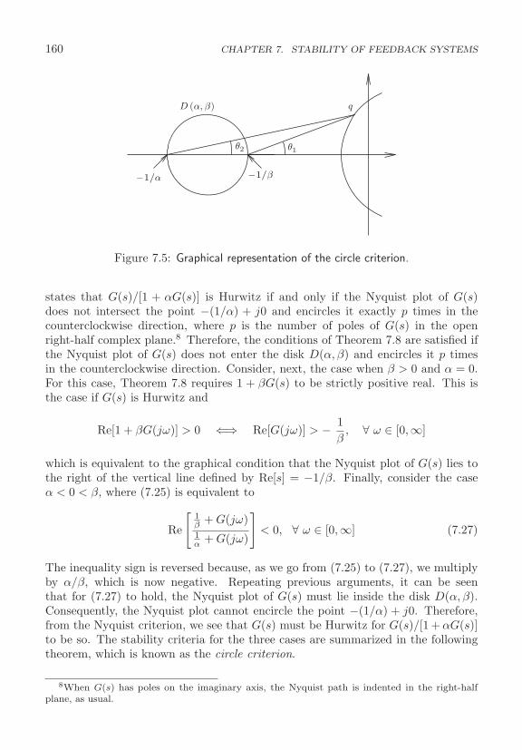
160 CHAPTER 7. STABILITY OF FEEDBACK SYSTEMS
q
θ2 θ1
D (α, β)
−1/α −1/β
Figure 7.5: Graphical representation of the circle criterion.
states that G(s)/[1 + αG(s)] is Hurwitz if and only if the Nyquist plot of G(s)does not intersect the point −(1/α) + j0 and encircles it exactly p times in thecounterclockwise direction, where p is the number of poles of G(s) in the openright-half complex plane.8 Therefore, the conditions of Theorem 7.8 are satisfied ifthe Nyquist plot of G(s) does not enter the disk D(α, β) and encircles it p timesin the counterclockwise direction. Consider, next, the case when β > 0 and α = 0.For this case, Theorem 7.8 requires 1 + βG(s) to be strictly positive real. This isthe case if G(s) is Hurwitz and
Re[1 + βG(jω)] > 0 ⇐⇒ Re[G(jω)] > − 1β
, ∀ ω ∈ [0,∞]
which is equivalent to the graphical condition that the Nyquist plot of G(s) lies tothe right of the vertical line defined by Re[s] = −1/β. Finally, consider the caseα < 0 < β, where (7.25) is equivalent to
Re
[1β + G(jω)1α + G(jω)
]< 0, ∀ ω ∈ [0,∞] (7.27)
The inequality sign is reversed because, as we go from (7.25) to (7.27), we multiplyby α/β, which is now negative. Repeating previous arguments, it can be seenthat for (7.27) to hold, the Nyquist plot of G(s) must lie inside the disk D(α, β).Consequently, the Nyquist plot cannot encircle the point −(1/α) + j0. Therefore,from the Nyquist criterion, we see that G(s) must be Hurwitz for G(s)/[1 + αG(s)]to be so. The stability criteria for the three cases are summarized in the followingtheorem, which is known as the circle criterion.
8When G(s) has poles on the imaginary axis, the Nyquist path is indented in the right-halfplane, as usual.
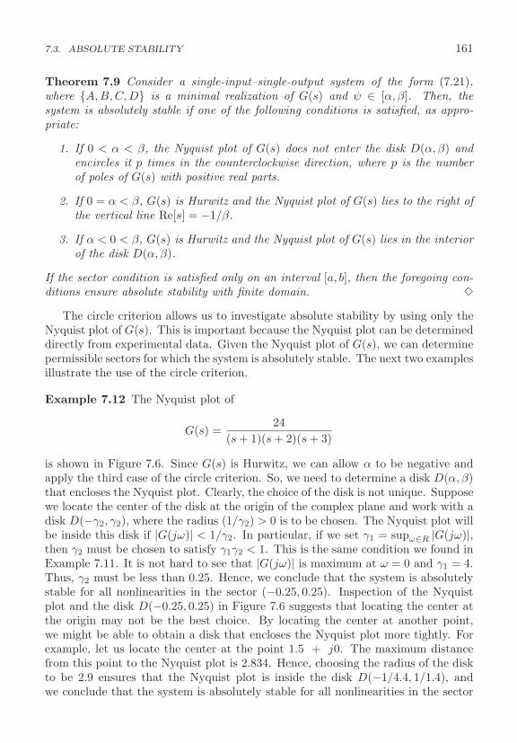
7.3. ABSOLUTE STABILITY 161
Theorem 7.9 Consider a single-input–single-output system of the form (7.21),where {A,B,C,D} is a minimal realization of G(s) and ψ ∈ [α, β]. Then, thesystem is absolutely stable if one of the following conditions is satisfied, as appro-priate:
1. If 0 < α < β, the Nyquist plot of G(s) does not enter the disk D(α, β) andencircles it p times in the counterclockwise direction, where p is the numberof poles of G(s) with positive real parts.
2. If 0 = α < β, G(s) is Hurwitz and the Nyquist plot of G(s) lies to the right ofthe vertical line Re[s] = −1/β.
3. If α < 0 < β, G(s) is Hurwitz and the Nyquist plot of G(s) lies in the interiorof the disk D(α, β).
If the sector condition is satisfied only on an interval [a, b], then the foregoing con-ditions ensure absolute stability with finite domain. �
The circle criterion allows us to investigate absolute stability by using only theNyquist plot of G(s). This is important because the Nyquist plot can be determineddirectly from experimental data. Given the Nyquist plot of G(s), we can determinepermissible sectors for which the system is absolutely stable. The next two examplesillustrate the use of the circle criterion.
Example 7.12 The Nyquist plot of
G(s) =24
(s + 1)(s + 2)(s + 3)
is shown in Figure 7.6. Since G(s) is Hurwitz, we can allow α to be negative andapply the third case of the circle criterion. So, we need to determine a disk D(α, β)that encloses the Nyquist plot. Clearly, the choice of the disk is not unique. Supposewe locate the center of the disk at the origin of the complex plane and work with adisk D(−γ2, γ2), where the radius (1/γ2) > 0 is to be chosen. The Nyquist plot willbe inside this disk if |G(jω)| < 1/γ2. In particular, if we set γ1 = supω∈R |G(jω)|,then γ2 must be chosen to satisfy γ1γ2 < 1. This is the same condition we found inExample 7.11. It is not hard to see that |G(jω)| is maximum at ω = 0 and γ1 = 4.Thus, γ2 must be less than 0.25. Hence, we conclude that the system is absolutelystable for all nonlinearities in the sector (−0.25, 0.25). Inspection of the Nyquistplot and the disk D(−0.25, 0.25) in Figure 7.6 suggests that locating the center atthe origin may not be the best choice. By locating the center at another point,we might be able to obtain a disk that encloses the Nyquist plot more tightly. Forexample, let us locate the center at the point 1.5 + j0. The maximum distancefrom this point to the Nyquist plot is 2.834. Hence, choosing the radius of the diskto be 2.9 ensures that the Nyquist plot is inside the disk D(−1/4.4, 1/1.4), andwe conclude that the system is absolutely stable for all nonlinearities in the sector

162 CHAPTER 7. STABILITY OF FEEDBACK SYSTEMS
−5 0 5−4
−2
0
2
4
6ImG
ReG
Figure 7.6: Nyquist plot for Exam-ple 7.12.
−4 −2 0−0.4
−0.2
0
0.2
0.4ImG
ReG
Figure 7.7: Nyquist plot for Exam-ple 7.13.
[−0.227, 0.714]. Comparing this sector with the previous one shows that by giving ina little bit on the lower bound of the sector, we achieve a significant improvement inthe upper bound. Clearly, there is still room for optimizing the choice of the centerof the disk. The point we wanted to show is that the graphical representation ofthe circle criterion gives a closer look at the problem, compared with the use ofnorm inequalities as in Example 7.11, which allows us to obtain less conservativeestimates of the sector. Another direction we can pursue is to restrict α to zero andapply the second case of the circle criterion. The Nyquist plot lies to the right of thevertical line Re[s] = −0.857. Hence, we can conclude that the system is absolutelystable for all nonlinearities in the sector [0, 1.166]. It gives the best estimate of β,which is achieved at the expense of limiting the nonlinearity to the first and thirdquadrants. To appreciate how this flexibility in using the circle criterion could beuseful in applications, let us suppose that we are interested in studying the stabilityof the system when ψ(y) = sat(y). The saturation nonlinearity belongs to thesector [0, 1]. Therefore, it is included in the sector [0, 1.166], but not in the sector(−0.25, 0.25) or [−0.227, 0.714]. �
Example 7.13 The transfer function
G(s) =24
(s − 1)(s + 2)(s + 3)
is not Hurwitz, since it has a pole in the open right-half plane. So, we must restrictα to be positive and apply the first case of the circle criterion. The Nyquist plot ofG(s) is shown in Figure 7.7. From the circle criterion, we know that the Nyquist plotmust encircle the disk D(α, β) once in the counterclockwise direction. Therefore,the disk has to be totally inside the left lobe of the plot. Let us locate the center ofthe disk at the point −3.2 + j0, about halfway between the two ends of the lobe onthe real axis. The minimum distance from this center to the Nyquist plot is 0.1688.Hence, choosing the radius to be 0.168, we conclude that the system is absolutelystable for all nonlinearities in the sector [0.2969, 0.3298]. �
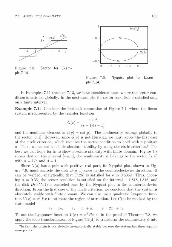
7.3. ABSOLUTE STABILITY 163
ya1−1−a
1
y/aψ (y)
Figure 7.8: Sector for Exam-ple 7.14.
−2 −1.5 −1 −0.5 0
−0.5
0
0.5
1ImG
ReG
Figure 7.9: Nyquist plot for Exam-ple 7.14.
In Examples 7.11 through 7.13, we have considered cases where the sector con-dition is satisfied globally. In the next example, the sector condition is satisfied onlyon a finite interval.
Example 7.14 Consider the feedback connection of Figure 7.4, where the linearsystem is represented by the transfer function
G(s) =s + 2
(s + 1)(s − 1)
and the nonlinear element is ψ(y) = sat(y). The nonlinearity belongs globally tothe sector [0, 1]. However, since G(s) is not Hurwitz, we must apply the first caseof the circle criterion, which requires the sector condition to hold with a positiveα. Thus, we cannot conclude absolute stability by using the circle criterion.9 Thebest we can hope for is to show absolute stability with finite domain. Figure 7.8shows that on the interval [−a, a], the nonlinearity ψ belongs to the sector [α, β]with α = 1/a and β = 1.
Since G(s) has a pole with positive real part, its Nyquist plot, shown in Fig-ure 7.9, must encircle the disk D(α, 1) once in the counterclockwise direction. Itcan be verified, analytically, that (7.25) is satisfied for α > 0.5359. Thus, choos-ing α = 0.55, the sector condition is satisfied on the interval [−1.818, 1.818] andthe disk D(0.55, 1) is encircled once by the Nyquist plot in the counterclockwisedirection. From the first case of the circle criterion, we conclude that the system isabsolutely stable with finite domain. We can also use a quadratic Lyapunov func-tion V (x) = xT Px to estimate the region of attraction. Let G(s) be realized by thestate model
x1 = x2, x2 = x1 + u, y = 2x1 + x2
To use the Lyapunov function V (x) = xT Px as in the proof of Theorem 7.8, weapply the loop transformation of Figure 7.3(d) to transform the nonlinearity ψ into
9In fact, the origin is not globally asymptotically stable because the system has three equilib-rium points.
164 CHAPTER 7. STABILITY OF FEEDBACK SYSTEMS
a passive nonlinearity. The loop transformation is given by
u = −αy + u = −0.55y + u, y = (β − α)y + u = 0.45y + u
and the transformed linear system is
x = Ax + Bu, y = Cx + Du
where
A =[
0 1−0.1 −0.55
], B =
[01
], C =
[0.9 0.45
], and D = 1
The matrix P is obtained by solving the Kalman–Yakubovich–Popov equations (5.13)–(5.15). From equation (5.15), W =
√2. Taking ε = 0.02, it can be verified that
equations (5.13)–(5.14) have two solutions, given by10
P1 =[
0.4946 0.48340.4834 1.0774
], L1 =
[0.2946 −0.4436
]and
P2 =[
0.7595 0.49200.4920 1.9426
], L2 =
[ −0.2885 1.0554]
Thus V1(x) = xT P1x and V2(x) = xT P2x are two different Lyapunov functions forthe system. For each Lyapunov function, we estimate the region of attraction by aset of the form {V (x) ≤ c} in the interior of {|y| ≤ 1.8181}. Noting that11
min{|y|=1.818}
V1(x) =(1.818)2
bT P−11 b
= 0.3445 and min{|y|=1.818}
V2(x) =(1.818)2
bT P−12 b
= 0.6212
where bT =[2 1
], we estimate the region of attraction by the sets {V1(x) ≤ 0.34}
and {V2(x) ≤ 0.62}, shown in Figure 7.10. According to Remark 3.1, the union ofthese two sets is an estimate of the region of attraction, which is bigger than theestimates obtained by the individual Lyapunov functions. �
7.3.2 Popov Criterion
Consider a special case of the system (7.21), given by
x = Ax + Bu, y = Cx ui = −ψi(yi), 1 ≤ i ≤ m (7.28)
where x ∈ Rn, u, y ∈ Rm, (A,B) is controllable, (A,C) is observable, and ψi isa locally Lipschitz memoryless nonlinearity that belongs to the sector [0, ki]. In
10The value of ε is chosen such that H(s−ε/2) is positive real and Hurwitz, where H(s) = C(sI−A)−1B + D. Then, P is calculated by solving a Riccati equation, as described in Exercise 5.14.
11See equation (B.3).

7.3. ABSOLUTE STABILITY 165
−1.5 −1 −0.5 0 0.5 1 1.51
−0.5
0
0.5
1V 2(x) = 0.62
V 1(x) = 0.34
y= −1.818
y= 1.818x2
x1
Figure 7.10: Region of attraction for Example 7.14.
this special case, the transfer function G(s) = C(sI − A)−1B is strictly properand ψ is time invariant and decoupled; that is, ψi(y) = ψi(yi). Since D = 0, thefeedback connection has a well-defined state model. The following theorem, knownas the multivariable Popov criterion, is proved by using a (Lure-type) Lyapunovfunction of the form V = 1
2xT Px +∑
γi
∫ yi
0ψi(σ) dσ, which is motivated by the
application of a loop transformation that transforms the system (7.28) into thefeedback connection of two passive dynamical systems.
Theorem 7.10 The system (7.28) is absolutely stable if, for 1 ≤ i ≤ m, ψi ∈[0, ki], 0 < ki ≤ ∞, and there exists a constant γi ≥ 0, with (1 + λkγi) �= 0for every eigenvalue λk of A, such that M + (I + sΓ)G(s) is strictly positive real,where Γ = diag(γ1, . . . , γm) and M = diag(1/k1, . . . , 1/km). If the sector conditionψi ∈ [0, ki] is satisfied only on a set Y ⊂ Rm, then the foregoing conditions ensureabsolute stability with finite domain. �
Proof: The loop transformation of Figure 7.11 results in a feedback connection ofH1 and H2, where H1 is a linear system whose transfer function is
M + (I + sΓ)G(s) = M + (I + sΓ)C(sI − A)−1B
= M + C(sI − A)−1B + ΓCs(sI − A)−1B
= M + C(sI − A)−1B + ΓC(sI − A + A)(sI − A)−1B
= M + (C + ΓCA)(sI − A)−1B + ΓCB
Thus, M + (I + sΓ)G(s) can be realized by the state model {A,B, C,D}, whereA = A, B = B, C = C + ΓCA, and D = M + ΓCB. Let λk be an eigenvalue of Aand vk be the associated eigenvector. Then
(C + ΓCA)vk = (C + ΓCλk)vk = (I + λkΓ)Cvk
The condition (1+λkγi) �= 0 implies that (A, C) is observable; hence, the realization{A,B, C,D} is minimal. If M + (I + sΓ)G(s) is strictly positive real, we can apply
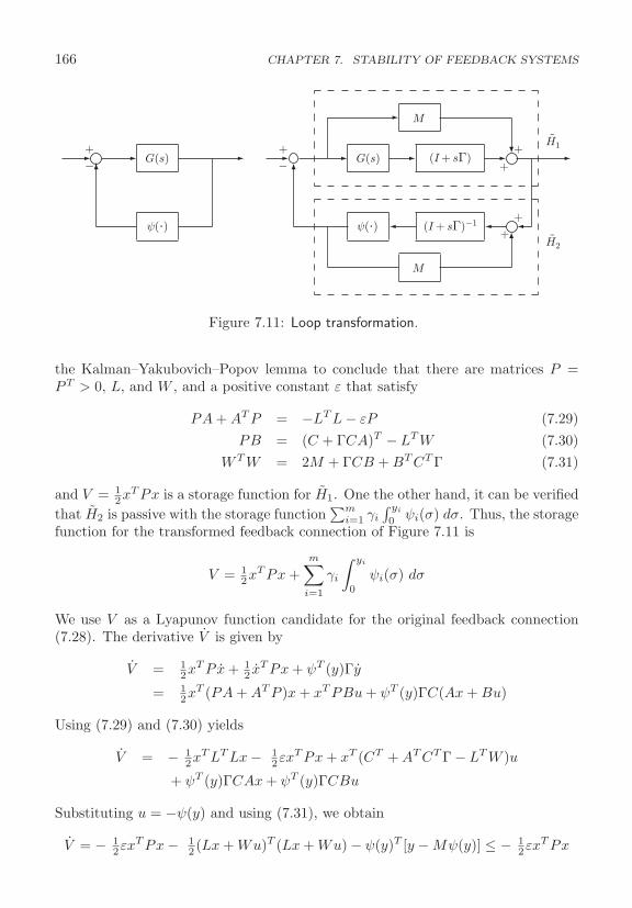
166 CHAPTER 7. STABILITY OF FEEDBACK SYSTEMS
+−
M
M
+−
++
++
G(s) G(s) (I+ sΓ)
(I+ sΓ)−1
H2
H1
ψ(·) ψ(·)
Figure 7.11: Loop transformation.
the Kalman–Yakubovich–Popov lemma to conclude that there are matrices P =PT > 0, L, and W , and a positive constant ε that satisfy
PA + AT P = −LT L − εP (7.29)PB = (C + ΓCA)T − LT W (7.30)
WT W = 2M + ΓCB + BT CT Γ (7.31)
and V = 12xT Px is a storage function for H1. One the other hand, it can be verified
that H2 is passive with the storage function∑m
i=1 γi
∫ yi
0ψi(σ) dσ. Thus, the storage
function for the transformed feedback connection of Figure 7.11 is
V = 12xT Px +
m∑i=1
γi
∫ yi
0
ψi(σ) dσ
We use V as a Lyapunov function candidate for the original feedback connection(7.28). The derivative V is given by
V = 12xT P x + 1
2 xT Px + ψT (y)Γy
= 12xT (PA + AT P )x + xT PBu + ψT (y)ΓC(Ax + Bu)
Using (7.29) and (7.30) yields
V = − 12xT LT Lx − 1
2εxT Px + xT (CT + AT CT Γ − LT W )u
+ ψT (y)ΓCAx + ψT (y)ΓCBu
Substituting u = −ψ(y) and using (7.31), we obtain
V = − 12εxT Px − 1
2 (Lx + Wu)T (Lx + Wu) − ψ(y)T [y − Mψ(y)] ≤ − 12εxT Px

7.3. ABSOLUTE STABILITY 167
slope= 1/γ ωIm[G(jω)]
Re[G(jω)]−1/k
Figure 7.12: Popov plot.
−0.5 0 0.5 1−1
−0.8
−0.6
−0.4
−0.2
0
0.2 ω ImG
ReG
slope= 1
Figure 7.13: Popov plot for Exam-ple 7.15.
which shows that the origin is globally asymptotically stable. If ψ satisfies the sectorcondition only for y ∈ Y , the foregoing analysis will be valid in some neighborhoodof the origin, showing that the origin is asymptotically stable. �
For M + (I + sΓ)G(s) to be strictly positive real, G(s) must be Hurwitz. Aswe have done in the circle criterion, this restriction on G(s) may be removed byperforming a loop transformation that replaces G(s) by G(s)[I + K1G(s)]−1. Wewill not repeat this idea in general, but will illustrate it by an example. In thecase m = 1, we can test strict positive realness of Z(s) = (1/k) + (1 + sγ)G(s)graphically. By Lemma 5.1, Z(s) is strictly positive real if G(s) is Hurwitz and
1k
+ Re[G(jω)] − γωIm[G(jω)] > 0, ∀ ω ∈ [0,∞] (7.32)
where G(jω) = Re[G(jω)] + jIm[G(jω)]. If we plot Re[G(jω)] versus ωIm[G(jω)]with ω as a parameter, then (7.32) is satisfied if the plot lies to the right of the linethat intercepts the point −(1/k) + j0 with slope 1/γ. (See Figure 7.12.) Such aplot is known as the Popov plot, in contrast to the Nyquist plot, which is a plotof Re[G(jω)] versus Im[G(jω)]. If (7.32) is satisfied only for ω ∈ [0,∞), while theleft-hand side approaches zero as ω tends to ∞, then we need to analytically verifythat
limω→∞ω2
{1k
+ Re[G(jω)] − γωIm[G(jω)]}
> 0
With γ = 0, condition (7.32) reduces to the circle criterion condition Re[G(jω)] >−1/k, which shows that, for the system (7.28), the conditions of the Popov criterionare weaker than those of the circle criterion. In other words, with γ > 0, absolutestability can be established under less stringent conditions.
Example 7.15 The two-dimensional system
x1 = x2, x2 = −x2 − h(y), y = x1

168 CHAPTER 7. STABILITY OF FEEDBACK SYSTEMS
would fit the form (7.28) if we took ψ = h, but the matrix A would not be Hurwitz.Adding and subtracting the term αy to the right-hand side of the second stateequation, where α > 0, and defining ψ(y) = h(y) − αy, the system takes the form(7.28), with
A =[
0 1−α −1
], B =
[01
], C =
[1 0
]Assume that h belongs to a sector [α, β], where β > α. Then, ψ belongs to thesector [0, k], where k = β − α. Condition (7.32) takes the form
1k
+α − ω2 + γω2
(α − ω2)2 + ω2> 0, ∀ ω ∈ [0,∞]
For all finite positive values of α and k, this inequality is satisfied by choosing γ > 1.Even with k = ∞, the foregoing inequality is satisfied for all ω ∈ [0,∞) and
limω→∞
ω2(α − ω2 + γω2)(α − ω2)2 + ω2
= γ − 1 > 0
Hence, the system is absolutely stable for all nonlinearities h in the sector [α,∞],where α can be arbitrarily small. Figure 7.13 shows the Popov plot of G(jω) forα = 1. The plot is drawn only for ω ≥ 0, since Re[G(jω)] and ωIm[G(jω)] areeven functions of ω. The Popov plot asymptotically approaches the line throughthe origin of unity slope from the right side. Therefore, it lies to the right of anyline of slope less than one that intersects the real axis at the origin and approachesit asymptotically as ω tends to ∞. To see the advantage of having γ > 0, let ustake γ = 0 and apply the circle criterion. From the second case of Theorem 7.9,the system is absolutely stable if the Nyquist plot of G(s) lies to the right of thevertical line defined by Re[s] = −1/k. Since a portion of the Nyquist plot lies inthe left-half plane, k cannot be arbitrarily large. The maximum permissible valueof k can be determined analytically from the condition
1k
+α − ω2
(α − ω2)2 + ω2> 0, ∀ ω ∈ [0,∞]
which yields k < 1 + 2√
α. Thus, using the circle criterion, we can only concludeabsolutely stability for nonlinearities h in the sector [α, 1 + α + 2
√α − ε], where
α > 0 and ε > 0 can be arbitrarily small. �
7.4 Exercises
7.1 Consider the feedback connection of Figure 7.1 with
H1 : x1 = −x1 + x2, x2 = −x31 − x2 + e1, y1 = x2
H2 : x3 = −x33 + e2, y2 = x3
3
Let u2 = 0, u = u1 be the input, and y = y1 be the output.
7.4. EXERCISES 169
(a) Show that the origin of the unforced system is globally asymptotically stable.
(b) Show that the mapping from u to y is finite-gain L2 stable.
7.2 Repeat the previous exercise with
H1 : x1 = x2, x2 = −x1 − ψ1(x2) + e1, y1 = x2
H2 : x3 = −aψ2(x3) + e2, y2 = ψ2(x3)
where ψ1 and ψ2 are locally Lipschitz functions, which satisfy zψ1(z) > bz2 andzψ2(z) > 0 for all z, and a and b are positive constants.
7.3 Consider the system
x1 = −x1 − x2 + u, x2 = ψ1(x1) − ψ2(x2), y = x1
where ψi belong to the sector [αi, βi] with βi > αi > 0, for i = 1, 2.
(a) Represent the state equation as the feedback connection of two strictly passivedynamical systems.
(b) Show that the origin of the unforced system is globally exponentially stable.
(c) Find V (x) ≥ 0 that satisfies the Hamilton Jacobi inequality with γ = β1/α1.
(d) Let u = −ψ3(y)+r, where ψ3 belongs to the sector [−δ, δ], with δ > 0. Find anupper bound on δ such that the mapping from r to y is finite-gain L2 stable.
7.4 Consider the system
x1 = −x1 + x2, x2 = −ψ1(x1) − x2 + u, y = x2
where ψ1 belongs to the sector [k,∞] for some k > 0, and let u = −ψ2(t, y) + r,where ψ2 is a time-varying memoryless function that belongs to the sector
[− 12 , 1
2
].
(a) Show that the origin of the unforced closed-loop system is globally uniformlyasymptotically stable.
(b) Show that the mapping from r to y is finite-gain L2 stable.
7.5 Consider the system
x1 = −x1 − x2 + u, x2 = x1 − x2 − x32, y = x1
(a) Show that the origin of the unforced system is globally exponentially stable.
(b) Show that the system is finite-gain L∞ stable and the L∞ gain is ≤ √2.

170 CHAPTER 7. STABILITY OF FEEDBACK SYSTEMS
(c) Let u = −ψ(y)+r, where ψ is locally Lipschitz and belongs to the sector [−δ, δ]with δ > 0. Find an upper bound on δ such that the system with input r andoutput y is finite-gain L∞ stable.
7.6 Consider the two-dimensional system
x = x/(1 + x2) + z, εz = −z + u, y = x
where the z-equation represents fast actuator dynamics. The feedback control istaken as u = −2x + r. Find an upper bound on ε such that the mapping from r toy is finite-gain Lp stable for every p ∈ [1,∞].
7.7 Consider the linear time-varying system x = [A + BE(t)C]x, where A isHurwitz and ‖E(t)‖ ≤ k ∀ t ≥ 0. Let γ = supω∈R σmax[C(jωI − A)−1B]. Findan upper bound on k such that the origin is uniformly asymptotically stable.
7.8 Consider the feedback connection of Figure 7.1 with
H1 : x1 = −x1+e1, x2 = x1−x2+e1, y1 = x1+x2 and H2 : y2 = ψ(e2)
where ψ is a locally Lipschitz function that satisfies yψ(y) ≥ 0 and |ψ(y)| ≤ 2 for ally, and ψ(y) = 0 for |y| ≤ 1. Show that the origin of the unforced system is globallyexponentially stable.
7.9 Consider the single-input system x = Ax+BM sat(u/M) in which the controlinput saturates at ±M . Let u = −Fx, where A−BF is Hurwitz. We use the circlecriterion to investigate asymptotic stability of the origin of the closed-loop system.
(a) Show that the closed-loop system can be represented in the form of Figure 7.4with G(s) = −F (sI − A + BF )−1B and ψ(y) = y − M sat(y/M).
(b) Show that the origin is globally asymptotically stable if Re[G(jω)] > −1 ∀ ω.
(c) If Re[G(jω)] > −β ∀ ω with β > 1, show that the origin is asymptotically stableand its region of attraction is estimated by {xT Px ≤ c}, where P satisfies
P (A − BF ) + (A − BF )T P = −LT L − εP, PB = −βFT −√
2LT
and c > 0 is chosen such that {xT Px ≤ c} ⊂ {|Fx| ≤ βM/(β − 1)}.
(d) Estimate the region of attraction when A =[
0 11 0
], B =
[01
],
F =[
2 1], and M = 1.
7.10 Consider the feedback connection of Figure 7.4. Use the circle and Popovcriteria to find a sector [α, β] for absolute stability when
(1) G(s) = 1/[(s + 2)(s − 1)] (2) G(s) = 1/[(s + 2)(s + 1)](3) G(s) = 2s/(s2 − 2s + 1) (4) G(s) = 2s/(s2 + 2s + 1)(5) G(s) = 1/(s + 1)3 (6) G(s) = (s − 1)/[(s + 1)(s + 2)](7) G(s) = (s + 2)/[(s2 − 1)(s + 4)] (8) G(s) = (s + 1)2/[(s + 2)(s − 1)2]
Chapter 8
Special Nonlinear Forms
The design of feedback control for nonlinear systems is simplified when the systemtakes one of certain special forms. Three such forms are presented in this chapter:the normal, controller, and observer forms.1 The normal form of Section 8.1 plays acentral role in the forthcoming chapters. It enables us to extend to nonlinear systemssome important notions in feedback control of linear systems, such as the relativedegree of a transfer function, its zeros, and the minimum phase property whenall the zeros have negative real parts. One of the fundamental tools in feedbackcontrol is the use of high-gain feedback to achieve disturbance rejection and lowsensitivity to model uncertainty.2 For linear systems, root locus analysis showsthat a minimum phase, relative-degree-one system can be stabilized by arbitrarilylarge feedback gain because, as the gain approaches infinity, one branch of the rootlocus approaches infinity on the negative real axis while the remaining branchesapproach the zeros of the system. The normal form enables us to show the sameproperty for nonlinear systems, as we shall see in Section 12.5.1.
The controller form of Section 8.2 is a special case of the normal form, but sig-nificant in its own sake because a nonlinear system in the controller form can beconverted into an equivalent controllable linear system by state feedback. There-fore, systems that can be transformed into the controller form are called feedbacklinearizable. The observer form of Section 8.3 reduces the design of a nonlinearobserver to a linear design problem.
8.1 Normal Form
Consider the n-dimensional, single-input–single-output system
x = f(x) + g(x)u, y = h(x) (8.1)
1This chapter is based mostly on [66].2See [34].
171
172 CHAPTER 8. SPECIAL NONLINEAR FORMS
where f , g, and h are sufficiently smooth in a domain D ⊂ Rn. The mappingsf : D → Rn and g : D → Rn are called vector fields on D. The derivative y is givenby
y =∂h
∂x[f(x) + g(x)u] def= Lfh(x) + Lgh(x) u
whereLfh(x) =
∂h
∂xf(x)
is called the Lie Derivative of h with respect to f or along f . This is the familiarnotion of the derivative of h along the trajectories of the system x = f(x). The newnotation is convenient when we repeat the calculation of the derivative with respectto the same vector field or a new one. For example, the following notation is used:
LgLfh(x) =∂(Lfh)
∂xg(x)
L2fh(x) = LfLfh(x) =
∂(Lfh)∂x
f(x)
Lkfh(x) = LfLk−1
f h(x) =∂(Lk−1
f h)∂x
f(x)
L0fh(x) = h(x)
If Lgh(x) = 0, then y = Lfh(x) is independent of u. If we continue to calculate thesecond derivative of y, denoted by y(2), we obtain
y(2) =∂(Lfh)
∂x[f(x) + g(x)u] = L2
fh(x) + LgLfh(x) u
Once again, if LgLfh(x) = 0, then y(2) = L2fh(x) is independent of u. Repeating
this process, we see that if h(x) satisfies
LgLi−1f h(x) = 0, for i = 1, 2, . . . , ρ − 1, and LgL
ρ−1f h(x) �= 0
for some integer ρ, then u does not appear in the equations of y, y, . . . , y(ρ−1) andappears in the equation of y(ρ) with a nonzero coefficient:
y(ρ) = Lρfh(x) + LgL
ρ−1f h(x) u
Such integer ρ has to be less than or equal to n,3 and is called the relative degreeof the system, according to the following definition.
Definition 8.1 The nonlinear system (8.1) has relative degree ρ, 1 ≤ ρ ≤ n, in anopen set R ⊂ D if, for all x ∈ R,
LgLi−1f h(x) = 0, for i = 1, 2, . . . , ρ − 1; LgL
ρ−1f h(x) �= 0 (8.2)
3See [74, Lemma C9] or [66, Lemma 4.1.1] for the proof that ρ ≤ n.

8.1. NORMAL FORM 173
If a system has relative degree ρ, then its input-output map can be converted intoa chain of integrators y(ρ) = v by the state feedback control
u =1
LgLρ−1f h(x)
(−Lρ
fh(x) + v)
Example 8.1 Consider the controlled van der Pol equation (A.13):
x1 = x2/ε, x2 = ε[−x1 + x2 − 13x3
2 + u]
with output y = x1. Calculating the derivatives of the output, we obtain
y = x1 = x2/ε, y = x2/ε = −x1 + x2 − 13x3
2 + u
Hence, the system has relative degree two in R2. For the output y = x2,
y = ε[−x1 + x2 − 13x3
2 + u]
and the system has relative degree one in R2. For the output y = 12 (ε2x2
1 + x22),
y = ε2x1x1 + x2x2 = εx1x2 + εx2[−x1 + x2 − 13x3
2 + u] = εx22 − (ε/3)x4
2 + εx2u
and the system has relative degree one in {x2 �= 0}. �
Example 8.2 The field-controlled DC motor (A.25) with δ = 0 and f�(x3) = bx3
is modeled by the state equation
x1 = d1(−x1 − x2x3 + Va), x2 = d2[−fe(x2) + u], x3 = d3(x1x2 − bx3)
where d1 to d3 are positive constants. For speed control, we choose the output asy = x3. The derivatives of the output are given by
y = x3 = d3(x1x2 − bx3)y = d3(x1x2 + x1x2 − bx3) = (· · · ) + d2d3x1u
The system has relative degree two in {x1 �= 0}. �
Example 8.3 Consider a linear system represented by the transfer function
H(s) =bmsm + bm−1s
m−1 + · · · + b0
sn + an−1sn−1 + · · · + a0
def=N(s)D(s)
where m < n and bm �= 0. A state model of the system can be taken as
x = Ax + Bu, y = Cx
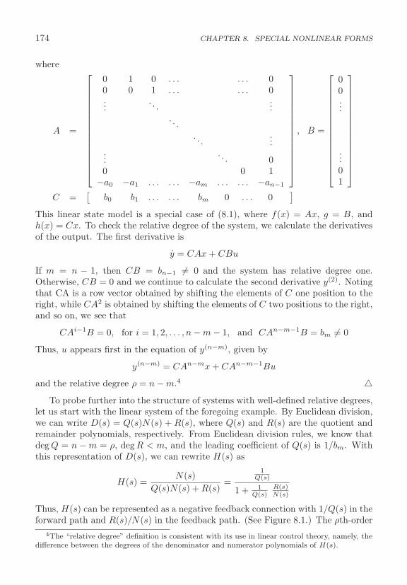
174 CHAPTER 8. SPECIAL NONLINEAR FORMS
where
A =
⎡⎢⎢⎢⎢⎢⎢⎢⎢⎢⎢⎢⎢⎢⎢⎣
0 1 0 . . . . . . 00 0 1 . . . . . . 0...
. . ....
. . .. . .
......
. . . 00 0 1
−a0 −a1 . . . . . . −am . . . . . . −an−1
⎤⎥⎥⎥⎥⎥⎥⎥⎥⎥⎥⎥⎥⎥⎥⎦
, B =
⎡⎢⎢⎢⎢⎢⎢⎢⎢⎢⎢⎢⎢⎢⎢⎣
00...
...01
⎤⎥⎥⎥⎥⎥⎥⎥⎥⎥⎥⎥⎥⎥⎥⎦
C =[
b0 b1 . . . . . . bm 0 . . . 0]
This linear state model is a special case of (8.1), where f(x) = Ax, g = B, andh(x) = Cx. To check the relative degree of the system, we calculate the derivativesof the output. The first derivative is
y = CAx + CBu
If m = n − 1, then CB = bn−1 �= 0 and the system has relative degree one.Otherwise, CB = 0 and we continue to calculate the second derivative y(2). Notingthat CA is a row vector obtained by shifting the elements of C one position to theright, while CA2 is obtained by shifting the elements of C two positions to the right,and so on, we see that
CAi−1B = 0, for i = 1, 2, . . . , n − m − 1, and CAn−m−1B = bm �= 0
Thus, u appears first in the equation of y(n−m), given by
y(n−m) = CAn−mx + CAn−m−1Bu
and the relative degree ρ = n − m.4 �To probe further into the structure of systems with well-defined relative degrees,
let us start with the linear system of the foregoing example. By Euclidean division,we can write D(s) = Q(s)N(s) + R(s), where Q(s) and R(s) are the quotient andremainder polynomials, respectively. From Euclidean division rules, we know thatdeg Q = n − m = ρ, deg R < m, and the leading coefficient of Q(s) is 1/bm. Withthis representation of D(s), we can rewrite H(s) as
H(s) =N(s)
Q(s)N(s) + R(s)=
1Q(s)
1 + 1Q(s)
R(s)N(s)
Thus, H(s) can be represented as a negative feedback connection with 1/Q(s) in theforward path and R(s)/N(s) in the feedback path. (See Figure 8.1.) The ρth-order
4The “relative degree” definition is consistent with its use in linear control theory, namely, thedifference between the degrees of the denominator and numerator polynomials of H(s).
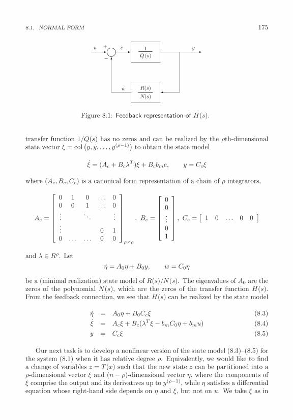
8.1. NORMAL FORM 175
u e y
w
+
−1
Q(s)
R(s)
N(s)
Figure 8.1: Feedback representation of H(s).
transfer function 1/Q(s) has no zeros and can be realized by the ρth-dimensionalstate vector ξ = col
(y, y, . . . , y(ρ−1)
)to obtain the state model
ξ = (Ac + BcλT )ξ + Bcbme, y = Ccξ
where (Ac, Bc, Cc) is a canonical form representation of a chain of ρ integrators,
Ac =
⎡⎢⎢⎢⎢⎢⎢⎣
0 1 0 . . . 00 0 1 . . . 0...
. . ....
... 0 10 . . . . . . 0 0
⎤⎥⎥⎥⎥⎥⎥⎦
ρ×ρ
, Bc =
⎡⎢⎢⎢⎢⎢⎣
00...01
⎤⎥⎥⎥⎥⎥⎦ , Cc =
[1 0 . . . 0 0
]
and λ ∈ Rρ. Let
η = A0η + B0y, w = C0η
be a (minimal realization) state model of R(s)/N(s). The eigenvalues of A0 are thezeros of the polynomial N(s), which are the zeros of the transfer function H(s).From the feedback connection, we see that H(s) can be realized by the state model
η = A0η + B0Ccξ (8.3)ξ = Acξ + Bc(λT ξ − bmC0η + bmu) (8.4)y = Ccξ (8.5)
Our next task is to develop a nonlinear version of the state model (8.3)–(8.5) forthe system (8.1) when it has relative degree ρ. Equivalently, we would like to finda change of variables z = T (x) such that the new state z can be partitioned into aρ-dimensional vector ξ and (n − ρ)-dimensional vector η, where the components ofξ comprise the output and its derivatives up to y(ρ−1), while η satisfies a differentialequation whose right-hand side depends on η and ξ, but not on u. We take ξ as in

176 CHAPTER 8. SPECIAL NONLINEAR FORMS
the linear case:
ξ =
⎡⎢⎢⎢⎣
yy(1)
...y(ρ−1)
⎤⎥⎥⎥⎦ =
⎡⎢⎢⎢⎣
h(x)Lfh(x)
...Lρ−1
f h(x)
⎤⎥⎥⎥⎦
When ρ = n, there is no η variable and the change of variables is given by
z = T (x) = col(h(x), Lfh(x), . . . , Ln−1
f h(x))
(8.6)
When ρ < n, the change of variables is taken as
z = T (x) =
⎡⎢⎢⎢⎢⎢⎢⎢⎢⎢⎢⎣
φ1(x)...
φn−ρ(x)−−−h(x)
...Lρ−1
f h(x)
⎤⎥⎥⎥⎥⎥⎥⎥⎥⎥⎥⎦
def=
⎡⎣ φ(x)
−−−H(x)
⎤⎦ def=
⎡⎣ η
−−−ξ
⎤⎦ (8.7)
where φ1 to φn−ρ are chosen such that T (x) is a diffeomorphism on a domainDx ⊂ R and
∂φi
∂xg(x) = 0, for 1 ≤ i ≤ n − ρ, ∀ x ∈ Dx (8.8)
so that the u term cancels out in
η =∂φ
∂x[f(x) + g(x)u]
The next theorem shows that the change of variables (8.6) or (8.7) is well defined,at least locally.5
Theorem 8.1 Consider the system (8.1) and suppose it has relative degree ρ ≤ nin R. If ρ = n, then for every x0 ∈ R, a neighborhood N of x0 exists such thatthe map T (x) of (8.6), restricted to N , is a diffeomorphism on N . If ρ < n, then,for every x0 ∈ R, a neighborhood N of x0 and continuously differentiable functionsφ1(x), . . . , φn−ρ(x) exist such that (8.8) is satisfied for all x ∈ N and the map T (x)of (8.7), restricted to N , is a diffeomorphism on N . �
When ρ < n, the change of variables (8.7) transforms (8.1) into
η = f0(η, ξ) (8.9)ξ = Acξ + Bc[L
ρfh(x) + LgL
ρ−1f h(x)u] (8.10)
y = Ccξ (8.11)5See [74, Theorem 13.1] or [66, Proposition 4.1.3] for the proof of Theorem 8.1. See [66, Section
9.1] for a global version and [66, Section 5.1] for a multiinput-multioutput version.
8.1. NORMAL FORM 177
where ξ ∈ Rρ, η ∈ Rn−ρ, (Ac, Bc, Cc) is a canonical form representation of a chainof ρ integrators, and
f0(η, ξ) =∂φ
∂xf(x)∣∣∣∣x=T−1(z)
(8.12)
We have kept Lρfh and LgL
ρ−1f h in (8.10) as functions of x because they are inde-
pendent of the choice of φ. When expressed in the new coordinates, (8.10) is givenby
ξ = Acξ + Bc[ψ(η, ξ) + γ(η, ξ)u]
where
ψ(η, ξ) = Lρfh(x)
∣∣∣x=T−1(z)
, γ(η, ξ) = LgLρ−1f h(x)
∣∣∣x=T−1(z)
If x∗ is an open-loop equilibrium point of (8.1), then (η∗, ξ∗), defined by
η∗ = φ(x∗), ξ∗ =[
h(x∗) 0 · · · 0]
is an equilibrium point of (8.9)–(8.10). If h(x∗) = 0, we can transform x∗ into theorigin point (η = 0, ξ = 0) by choosing φ(x) such that φ(x∗) = 0, which is alwayspossible because adding a constant to a function φi that satisfies (8.8) does notalter this condition, nor the property that T (x) is a diffeomorphism.
Equations (8.9) through (8.11) are said to be in the normal form. This formdecomposes the system into internal dynamics (8.9) and external dynamics (8.10)–(8.11). The state feedback control
u =1
LgLρ−1f h(x)
[−Lρ
fh(x) + v]
converts the external dynamics into a chain of ρ integrators, y(ρ) = v, and makesthe internal dynamics unobservable from the output y. When y(t) is identicallyzero, so is ξ(t). Setting ξ = 0 in (8.9) results in
η = f0(η, 0) (8.13)
which is called the zero dynamics. The system is said to be minimum phase if(8.13) has an asymptotically stable equilibrium point in the domain of interest. Inparticular, if T (x) is chosen such that the origin (η = 0, ξ = 0) is an equilibriumpoint of (8.9)–(8.11), then the system is minimum phase if the origin of the zerodynamics (8.13) is asymptotically stable. It is useful to know that the zero dynamicscan be characterized in the original coordinates. Noting that
y(t) ≡ 0 ⇒ ξ(t) ≡ 0 ⇒ u(t) ≡ − Lρfh(x(t))
LgLρ−1f h(x(t))

178 CHAPTER 8. SPECIAL NONLINEAR FORMS
we see that if the output is identically zero, the solution of the state equation mustbe confined to the set
Z∗ = {x ∈ R | h(x) = Lfh(x) = · · · = Lρ−1f h(x) = 0}
and the input must be
u = u∗(x) def= − Lρfh(x)
LgLρ−1f h(x)
∣∣∣∣∣x∈Z∗
The restricted motion of the system is described by
x = f∗(x) def=
[f(x) − g(x)
Lρfh(x)
LgLρ−1f h(x)
]x∈Z∗
In the special case ρ = n, the normal form reduces to
z = Acz + Bc[Lnf h(x) + LgL
n−1f h(x)u], y = Ccz (8.14)
In this case, the system has no zero dynamics and, by default, is said to be minimumphase.
Example 8.4 Consider the controlled van der Pol equation (A.13):
x1 = x2/ε, x2 = ε[−x1 + x2 − 13x3
2 + u], y = x2
We have seen in Example 8.1 that the system has relative degree one in R2. Takingξ = y and η = x1, we see that the system is already in the normal form. The zerodynamics are given by the equation x1 = 0, which does not have an asymptoticallystable equilibrium point. Hence, the system is not minimum phase. �
Example 8.5 The system
x1 = −x1 +2 + x2
3
1 + x23
u, x2 = x3, x3 = x1x3 + u, y = x2
has an open-loop equilibrium point at the origin. The derivatives of the output are
y = x2 = x3, y = x3 = x1x3 + u
Therefore, the system has relative degree two in R3. To characterize the zerodynamics, restrict x to Z∗ = {x2 = x3 = 0} and take
u = u∗(x) = − L2fh(x)
LgLfh(x)
∣∣∣∣∣x∈Z∗
= −x1x3
∣∣∣∣∣∣x∈Z∗
= 0
8.2. CONTROLLER FORM 179
This process yields x1 = −x1, which shows that the system is minimum phase. Totransform the system into the normal form, we want to choose φ(x) such that
φ(0) = 0,∂φ
∂xg(x) = 0
and T (x) = col (φ(x), x2, x3) is a diffeomorphism on some domain containing theorigin. The partial differential equation
∂φ
∂x1· 2 + x2
3
1 + x23
+∂φ
∂x3= 0, φ(0) = 0
can be solved by separation of variables to obtain φ(x) = x1 − x3 − tan−1 x3.The mapping T (x) is a global diffeomorphism because it is proper and [∂T/∂x] isnonsingular for all x. Thus, the normal form
η = − (η + ξ2 + tan−1 ξ2
)(1 +
2 + ξ22
1 + ξ22
ξ2
)ξ1 = ξ2
ξ2 =(η + ξ2 + tan−1 ξ2
)ξ2 + u
y = ξ1
is defined globally. �
Example 8.6 The field-controlled DC motor of Example 8.2 has relative degreetwo in R = {x1 = 0} with h = x3 and Lfh = d3(x1x2 − bx3). To characterize thezero dynamics, restrict x to
Z∗ = {x ∈ R | x3 = 0 and x1x2 − bx3 = 0} = {x ∈ R | x2 = x3 = 0}
and take u = u∗(x), to obtain x1 = d1(−x1 + Va). The zero dynamics have anasymptotically stable equilibrium point at x1 = Va. Hence, the system is min-imum phase. To transform it into the normal form, we want to find a functionφ(x) such that [∂φ/∂x]g = d2∂φ/∂x2 = 0 and T = col (φ(x), x3, d3(x1x2 − bx3))is a diffeomorphism on some domain Dx ⊂ R. The choice φ(x) = x1 − Va satis-fies ∂φ/∂x2 = 0, makes T (x) a diffeomorphism on {x1 > 0}, and transforms theequilibrium point of the zero dynamics to the origin. �
8.2 Controller Form
A nonlinear system is in the controller form if its state model is given by
x = Ax + B[ψ(x) + γ(x)u] (8.15)

180 CHAPTER 8. SPECIAL NONLINEAR FORMS
where (A,B) is controllable and γ(x) is a nonsingular matrix for all x in the domainof interest. The system (8.15) can be converted into the controllable linear system
x = Ax + Bv
by the state feedback control
u = γ−1(x)[−ψ(x) + v]
where γ−1(x) is the inverse matrix of γ(x). Therefore, any system that can berepresented in the controller form is said to be feedback linearizable.
Example 8.7 An m-link robot is modeled by (A.35):
x1 = x2, x2 = M−1(x1)[u − C(x1, x2)x2 − Dx2 − g(x1)]
Taking x = col (x1, x2), the state model takes the form (8.15) with
A =[
0 Im
0 0
], B =
[0
Im
], ψ = −M−1(Cx2 + Dx2 + g), γ = M−1
�Even if the state model is not in the controller form, the system will be feedbacklinearizable if it can be transformed into that form. In this section, we characterizethe class of feedback linearizable single-input systems6
x = f(x) + g(x)u (8.16)
where f and g are sufficiently smooth vector fields on a domain D ⊂ Rn. Fromthe previous section we see that the system (8.16) is feedback linearizable in aneighborhood of x0 ∈ D if a (sufficiently smooth) function h exists such that thesystem
x = f(x) + g(x)u, y = h(x) (8.17)
has relative degree n in a neighborhood of x0. Theorem 8.1 ensures that the map
T (x) = col(h(x), Lfh(x), . . . , Ln−1
f h(x))
restricted to a neighborhood N of x0, is a diffeomorphism on N and the change ofvariables z = T (x) transforms the system into the normal form
z = Acz + Bc[ψ(z) + γ(z)u], y = Ccz
where (Ac, Bc, Cc) is a canonical form representation of a chain of n integrators. Onthe other hand, if (8.16) is feedback linearizable in a neighborhood N of x0 ∈ D,then there is a change of variables ζ = S(x) that transforms the system into
ζ = Aζ + B[ψ(ζ) + γ(ζ)u]6See [66, Chapter 5] for multi-input systems.
8.2. CONTROLLER FORM 181
where (A,B) is controllable and γ(ζ) = 0 in S(N). For any controllable pair (A,B),we can find a nonsingular matrix M that transforms (A,B) into the controllablecanonical form:7 MAM−1 = Ac + Bcλ
T ; MB = Bc. The change of variables
z = Mζ = MS(x) def= T (x)
transforms (8.16) intoz = Acz + Bc[ψ(z) + γ(z)u]
where γ(z) = γ(M−1z) and ψ(z) = ψ(M−1z) + λT z.
In summary, the system (8.16) is feedback linearizable in a neighborhood ofx0 ∈ D if and only if a (sufficiently smooth) function h(x) exists such that the system(8.17) has relative degree n in a domain Dx ⊂ D, with x0 ∈ Dx, or, equivalently, hsatisfies the partial differential equations
LgLi−1f h(x) = 0, i = 1, 2, . . . , n − 1 (8.18)
subject to the conditionLgL
n−1f h(x) = 0 (8.19)
for all x ∈ Dx. The existence of h can be characterized by necessary and sufficientconditions on the vector fields f and g. These conditions use the notions of Liebrackets and involutive distributions, which we introduce next.
For two vector fields f and g on D ⊂ Rn, the Lie bracket [f, g] is a third vectorfield defined by
[f, g](x) =∂g
∂xf(x) − ∂f
∂xg(x)
where [∂g/∂x] and [∂f/∂x] are Jacobian matrices. The Lie bracket [f, g](x) isinvariant under the change of variables z = T (x) in the sense that if
f(z) =∂T
∂xf(x)∣∣∣∣x=T−1(z)
and g(z) =∂T
∂xg(x)∣∣∣∣x=T−1(z)
then8
[f , g](z) =∂T
∂x[f, g](x)
∣∣∣∣x=T−1(z)
We may repeat bracketing of g with f . The following notation is used to simplifythis process:
ad0fg(x) = g(x)
adfg(x) = [f, g](x)adk
fg(x) = [f, adk−1f g](x), k ≥ 1
It is obvious that [f, g] = −[g, f ] and for constant vector fields f and g, [f, g] = 0.7See, for example, [114].8See [98, Proposition 2.30] for the proof of this property.
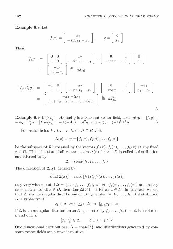
182 CHAPTER 8. SPECIAL NONLINEAR FORMS
Example 8.8 Let
f(x) =[
x2
− sin x1 − x2
], g =
[0x1
]Then,
[f, g] =[
0 01 0
] [x2
− sin x1 − x2
]−[
0 1− cos x1 −1
] [0x1
]
=[ −x1
x1 + x2
]def= adfg
[f, adfg] =[ −1 0
1 1
] [x2
− sin x1 − x2
]−[
0 1− cos x1 −1
] [ −x1
x1 + x2
]
=[ −x1 − 2x2
x1 + x2 − sin x1 − x1 cos x1
]def= ad2
fg
�Example 8.9 If f(x) = Ax and g is a constant vector field, then adfg = [f, g] =−Ag, ad2
fg = [f, adfg] = −A(−Ag) = A2g, and adkfg = (−1)kAkg. �
For vector fields f1, f2, . . . , fk on D ⊂ Rn, let
Δ(x) = span{f1(x), f2(x), . . . , fk(x)}be the subspace of Rn spanned by the vectors f1(x), f2(x), . . . , fk(x) at any fixedx ∈ D. The collection of all vector spaces Δ(x) for x ∈ D is called a distributionand referred to by
Δ = span{f1, f2, . . . , fk}The dimension of Δ(x), defined by
dim(Δ(x)) = rank [f1(x), f2(x), . . . , fk(x)]
may vary with x, but if Δ = span{f1, . . . , fk}, where {f1(x), . . . , fk(x)} are linearlyindependent for all x ∈ D, then dim(Δ(x)) = k for all x ∈ D. In this case, we saythat Δ is a nonsingular distribution on D, generated by f1, . . . , fk. A distributionΔ is involutive if
g1 ∈ Δ and g2 ∈ Δ ⇒ [g1, g2] ∈ Δ
If Δ is a nonsingular distribution on D, generated by f1, . . . , fk, then Δ is involutiveif and only if
[fi, fj ] ∈ Δ, ∀ 1 ≤ i, j ≤ k
One dimensional distributions, Δ = span{f}, and distributions generated by con-stant vector fields are always involutive.
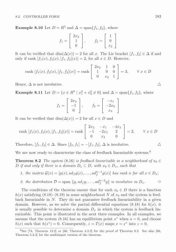
8.2. CONTROLLER FORM 183
Example 8.10 Let D = R3 and Δ = span{f1, f2}, where
f1 =
⎡⎣ 2x2
10
⎤⎦ , f2 =
⎡⎣ 1
0x2
⎤⎦
It can be verified that dim(Δ(x)) = 2 for all x. The Lie bracket [f1, f2] ∈ Δ if andonly if rank [f1(x), f2(x), [f1, f2](x)] = 2, for all x ∈ D. However,
rank [f1(x), f2(x), [f1, f2](x)] = rank
⎡⎣ 2x2 1 0
1 0 00 x2 1
⎤⎦ = 3, ∀ x ∈ D
Hence, Δ is not involutive. �Example 8.11 Let D = {x ∈ R3 | x2
1 + x23 = 0} and Δ = span{f1, f2}, where
f1 =
⎡⎣ 2x3
−10
⎤⎦ , f2 =
⎡⎣ −x1
−2x2
x3
⎤⎦
It can be verified that dim(Δ(x)) = 2 for all x ∈ D and
rank [f1(x), f2(x), [f1, f2](x)] = rank
⎡⎣ 2x3 −x1 −4x3
−1 −2x2 20 x3 0
⎤⎦ = 2, ∀ x ∈ D
Therefore, [f1, f2] ∈ Δ. Since [f2, f1] = −[f1, f2], Δ is involutive. �We are now ready to characterize the class of feedback linearizable systems.9
Theorem 8.2 The system (8.16) is feedback linearizable in a neighborhood of x0 ∈D if and only if there is a domain Dx ⊂ D, with x0 ∈ Dx, such that
1. the matrix G(x) = [g(x), adfg(x), . . . , adn−1f g(x)] has rank n for all x ∈ Dx;
2. the distribution D = span {g, adfg, . . . , adn−2f g} is involutive in Dx. �
The conditions of the theorem ensure that for each x0 ∈ D there is a functionh(x) satisfying (8.18)–(8.19) in some neighborhood N of x0 and the system is feed-back linearizable in N . They do not guarantee feedback linearizability in a givendomain. However, as we solve the partial differential equations (8.18) for h(x), itis usually possible to determine a domain Dx in which the system is feedback lin-earizable. This point is illustrated in the next three examples. In all examples, weassume that the system (8.16) has an equilibrium point x∗ when u = 0, and chooseh(x) such that h(x∗) = 0. Consequently, z = T (x) maps x = x∗ into z = 0.
9See [74, Theorem 13.2] or [66, Theorem 4.2.3] for the proof of Theorem 8.2. See also [66,Theorem 5.2.3] for the multiinput version of the theorem.
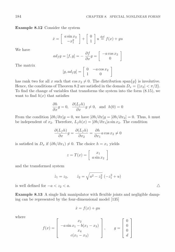
184 CHAPTER 8. SPECIAL NONLINEAR FORMS
Example 8.12 Consider the system
x =[
a sin x2
−x21
]+[
01
]u
def= f(x) + gu
We have
adfg = [f, g] = − ∂f
∂xg =[ −a cos x2
0
]The matrix
[g, adfg] =[
0 −a cos x2
1 0
]has rank two for all x such that cos x2 = 0. The distribution span{g} is involutive.Hence, the conditions of Theorem 8.2 are satisfied in the domain Dx = {|x2| < π/2}.To find the change of variables that transforms the system into the form (8.15), wewant to find h(x) that satisfies
∂h
∂xg = 0,
∂(Lfh)∂x
g = 0, and h(0) = 0
From the condition [∂h/∂x]g = 0, we have [∂h/∂x]g = [∂h/∂x2] = 0. Thus, h mustbe independent of x2. Therefore, Lfh(x) = [∂h/∂x1]a sin x2. The condition
∂(Lfh)∂x
g =∂(Lfh)
∂x2=
∂h
∂x1a cos x2 = 0
is satisfied in Dx if (∂h/∂x1) = 0. The choice h = x1 yields
z = T (x) =[
x1
a sin x2
]
and the transformed system
z1 = z2, z2 =√
a2 − z22 (−z2
1 + u)
is well defined for −a < z2 < a. �
Example 8.13 A single link manipulator with flexible joints and negligible damp-ing can be represented by the four-dimensional model [135]
x = f(x) + gu
where
f(x) =
⎡⎢⎢⎣
x2
−a sin x1 − b(x1 − x3)x4
c(x1 − x3)
⎤⎥⎥⎦ , g =
⎡⎢⎢⎣
000d
⎤⎥⎥⎦

8.2. CONTROLLER FORM 185
and a, b, c, and d are positive constants. The unforced system has an equilibriumpoint at x = 0. We have
adfg = [f, g] = − ∂f
∂xg =
⎡⎢⎢⎣
00−d0
⎤⎥⎥⎦ , ad2
fg = [f, adfg] = − ∂f
∂xadfg =
⎡⎢⎢⎣
0bd0
−cd
⎤⎥⎥⎦
ad3fg = [f, ad2
fg] = − ∂f
∂xad2
fg =
⎡⎢⎢⎣
−bd0cd0
⎤⎥⎥⎦
The matrix
[g, adfg, ad2fg, ad3
fg] =
⎡⎢⎢⎣
0 0 0 −bd0 0 bd 00 −d 0 cdd 0 −cd 0
⎤⎥⎥⎦
has full rank for all x ∈ R4. The distribution span(g, adfg, ad2fg) is involutive since
g, adfg, and ad2fg are constant vector fields. Thus, the conditions of Theorem 8.2
are satisfied for all x ∈ R4. To transform the system into the controller form, wewant to find h(x) that satisfies
∂(Li−1f h)∂x
g = 0, i = 1, 2, 3,∂(L3
fh)∂x
g = 0, and h(0) = 0
From the condition [∂h/∂x]g = 0, we have (∂h/∂x4) = 0, so we must choose hindependent of x4. Therefore,
Lfh(x) =∂h
∂x1x2 +
∂h
∂x2[−a sin x1 − b(x1 − x3)] +
∂h
∂x3x4
From the condition [∂(Lfh)/∂x]g = 0, we have
∂(Lfh)∂x4
= 0 ⇒ ∂h
∂x3= 0
So, we choose h independent of x3. Therefore, Lfh simplifies to
Lfh(x) =∂h
∂x1x2 +
∂h
∂x2[−a sin x1 − b(x1 − x3)]
and
L2fh(x) =
∂(Lfh)∂x1
x2 +∂(Lfh)
∂x2[−a sin x1 − b(x1 − x3)] +
∂(Lfh)∂x3
x4
186 CHAPTER 8. SPECIAL NONLINEAR FORMS
Finally,∂(L2
fh)∂x4
= 0 ⇒ ∂(Lfh)∂x3
= 0 ⇒ ∂h
∂x2= 0
and we choose h independent of x2. Hence,
L3fh(x) =
∂(L2fh)
∂x1x2 +
∂(L2fh)
∂x2[−a sin x1 − b(x1 − x3)] +
∂(L2fh)
∂x3x4
and the condition [∂(L3fh)/∂x]g = 0 is satisfied whenever (∂h/∂x1) = 0. Therefore,
we take h(x) = x1. The change of variables
z1 = h(x) = x1
z2 = Lfh(x) = x2
z3 = L2fh(x) = −a sin x1 − b(x1 − x3)
z4 = L3fh(x) = −ax2 cos x1 − b(x2 − x4)
transforms the system into the controller form
z1 = z2, z2 = z3, z3 = z4, z4 = −(a cos z1 + b + c)z3 + a(z22 − c) sin z1 + bdu
Unlike the previous example, in the current one the state equation in the z-coordinatesis valid globally because z = T (x) is a global diffeomorphism. �Example 8.14 The field-controlled DC motor (A.25) with δ = 0 and f�(x3) = bx3
is modeled by x = f(x) + gu, where
f =
⎡⎣d1(−x1 − x2x3 + Va)
−d2fe(x2)d3(x1x2 − bx3)
⎤⎦ , g =
⎡⎣ 0
d2
0
⎤⎦
in which d1 to d3 and Va are positive and b ≥ 0. Assume that fe(x2) is twicecontinuously differentiable in an open interval J ⊂ R. We have
adfg =
⎡⎣ d1d2x3
d22f
′e(x2)
−d2d3x1
⎤⎦ ; ad2
fg =
⎡⎣ d1d2x3(d1 + d2f
′e(x2) − bd3)
d32(f
′e(x2))2 − d3
2f2(x2)f ′′e (x2)
d1d2d3(x1 − Va) − d22d3x1f
′e(x2) − bd2d
23x1
⎤⎦
detG = det[g, adfg, ad2fg] = −2d2
1d32d3x3(x1 − a)(1 − bd3/d1)
where a = 12Va/(1 − bd3/d1). We assume that bd3/d1 = bTa/Tm < 1 so that a > 0,
which is reasonable since Ta is typically much smaller than Tm. Hence, G has rankthree for x1 = a and x3 = 0. The distribution D = span{g, adfg} is involutive if[g, adfg] ∈ D. We have
[g, adfg] =∂(adfg)
∂xg =
⎡⎣ 0 0 d1d2
0 d22f
′′e (x2) 0
−d2d3 0 0
⎤⎦⎡⎣ 0
d2
0
⎤⎦ = d2
2f′′e (x2)g
8.3. OBSERVER FORM 187
Hence, D is involutive and the conditions of Theorem 8.2 are satisfied in the domainDx = {x1 > a, x2 ∈ J, x3 > 0}. We proceed now to find a function h that satisfies(8.18) and (8.19). We take the desired operating speed as ω0 > 0, which is achievedat the equilibrium point x∗ = col (x∗
1, x∗2, x
∗3), where x∗
1 = (Va +√
V 2a − 4bω2
0)/2,x∗
2 = bω0/x∗1, and x∗
3 = ω0. We assume that V 2a > 4bω2
0 , x∗1 > a, and x∗
2 ∈ J . Wewant to find h(x) that satisfies
∂h
∂xg = 0;
∂(Lfh)∂x
g = 0;∂(L2
fh)∂x
g = 0
with h(x∗) = 0. From the condition [∂h/∂x]g = 0 ⇔ ∂h/∂x2 = 0, we see that hmust be independent of x2. Therefore,
Lfh(x) =∂h
∂x1d1(−x1 − x2x3 + Va) +
∂h
∂x3d3(x1x2 − bx3)
From the condition [∂(Lfh)/∂x]g = 0 ⇔ ∂(Lfh)/∂x2 = 0, obtain
−d1x3∂h
∂x1+ d3x1
∂h
∂x3= 0
which is satisfied by h = d3x21 + d1x
23 + c and we choose c = −d3(x∗
1)2 − d1(x∗
3)2 to
satisfy the condition h(x∗) = 0. With this choice of h, Lfh and L2fh are given by
Lfh(x) = 2d1d3x1(Va − x1) − 2bd1d3x23
L2fh(x) = 2d2
1d3(Va − 2x1)(−x1 − x2x3 + Va) − 4bd1d23x3(x1x2 − bx3)
Hence,∂(L2
fh)∂x
g = d2
∂(L2fh)
∂x2= 4d2
1d2d3(1 − bd3/d1)x3(x1 − a)
and the condition [∂(L2fh)/∂x]g = 0 is satisfied in Dx. �
8.3 Observer Form
A nonlinear system represented by
x = Ax + ψ(u, y), y = Cx (8.20)
where (A,C) is observable, is said to be in the observer form. Suppose the input uand output y are available on line, but not the state x. Assuming that the matricesA and C and the nonlinear function ψ(u, y) are known, we can implement thenonlinear observer
˙x = Ax + ψ(u, y) + H(y − Cx)
188 CHAPTER 8. SPECIAL NONLINEAR FORMS
to estimate x by x. The estimation error x = x − x satisfies the linear equation
˙x = (A − HC)x
Because (A,C) is observable, we can design H to assign the eigenvalues of A−HCin the open left-half plane, ensuring that limt→∞x(t) = 0. The next two examplesshow physical systems whose models are in the observer form.
Example 8.15 A single link manipulator with flexible joints and negligible damp-ing can be represented by the model [135]
x =
⎡⎢⎢⎣
x2
−a sin x1 − b(x1 − x3)x4
c(x1 − x3)
⎤⎥⎥⎦+
⎡⎢⎢⎣
000d
⎤⎥⎥⎦u
where a, b, c, and d are positive constants. Taking y = x1 as the output, it can beseen that the system is in the form (8.20) with
A =
⎡⎢⎢⎣
0 1 0 0−b 0 b 00 0 0 1c 0 −c 0
⎤⎥⎥⎦ , ψ =
⎡⎢⎢⎣
0−a sin y
0du
⎤⎥⎥⎦ , CT =
⎡⎢⎢⎣
1000
⎤⎥⎥⎦
and that (A,C) is observable. �Example 8.16 In equation (A.47), the inverted pendulum is modeled by
x1 = x2, x2 = a(sin x1 + u cos x1)
Taking y = x1 as the output, the system is in the observer form (8.20) with
A =[
0 10 0
], ψ =
[0
a(sin y + u cos y)
], CT =
[10
]�
In general, we may have to perform a change of variables to bring a systeminto the observer form, if possible. In this section we consider the n-dimensionalsingle-output nonlinear system
x = f(x) +m∑
i=1
gi(x)ui, y = h(x) (8.21)
where f , h, and g1 to gm are smooth functions in a domain D ⊂ Rn, and studythe existence of a diffeomorphism T (x) such that the change of variables z = T (x)transforms the system (8.21) into the observer form
z = Acz + φ(y) +m∑
i=1
γi(y)ui, y = Ccz (8.22)
8.3. OBSERVER FORM 189
where
Ac =
⎡⎢⎢⎢⎢⎢⎢⎣
0 1 0 . . . 00 0 1 . . . 0...
. . ....
... 0 10 . . . . . . 0 0
⎤⎥⎥⎥⎥⎥⎥⎦ , Cc =
[1 0 . . . 0 0
]
There is no loss of generality in taking (Ac, Cc) in the observable canonical formsince any observable pair (A,C) can be transformed into the observable canonicalform by a similarity transformation. We start by setting u = 0 and study theexistence of a change of variables that transforms the system
x = f(x), y = h(x) (8.23)
into the observer formz = Acz + φ(y), y = Ccz (8.24)
Define the map Φ(x) by
Φ(x) = col(h(x), Lfh(x), . . . , Ln−1
f h(x))
and note that the existence of a diffeomorphism that transforms the system (8.23)into the form (8.24) is possible only if the Jacobian matrix [∂Φ/∂x] is nonsingularover the domain of interest. This is so because, in the z-coordinates,
Φ(z) = Φ(x)|x=T−1(z) = col(h(z), Lf h(z), . . . , Ln−1
fh(z))
where f(z) = Acz + φ(Ccz), h(z) = Ccz, and the Jacobian matrix
∂Φ∂z
=
⎡⎢⎢⎢⎢⎢⎣
1 0 · · · 0∗ 1 0 0...
...∗ · · · ∗ 1 0∗ · · · ∗ 1
⎤⎥⎥⎥⎥⎥⎦
is nonsingular. By the chain rule, [∂Φ/∂z] = [∂Φ/∂x][∂T−1/∂z] and the Jacobianmatrix [∂T−1/∂z] is nonsingular because T is a diffeomorphism. Therefore, [∂Φ/∂x]is nonsingular. This implies that Φ(x) is a diffeomorphism. Noting that
Φ(x) = col(y, y, . . . , y(n−1))
we see that the system (8.23) is instantaneously observable because its state x canbe recovered from the output and its derivatives using the inverse of Φ.
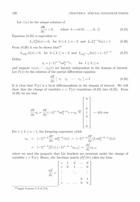
190 CHAPTER 8. SPECIAL NONLINEAR FORMS
Let τ(x) be the unique solution of
∂Φ∂x
τ = b, where b = col (0, . . . , 0, 1) (8.25)
Equation (8.25) is equivalent to
LτLkfh(x) = 0, for 0 ≤ k ≤ n − 2 and LτLn−1
f h(x) = 1 (8.26)
From (8.26) it can be shown that10
Ladkf τh(x) = 0, for 0 ≤ k ≤ n − 2 and Ladn−1
f τh(x) = (−1)n−1 (8.27)
Defineτk = (−1)n−kadn−k
f τ, for 1 ≤ k ≤ n
and suppose τ1(x), · · · , τn(x) are linearly independent in the domain of interest.Let T (x) be the solution of the partial differential equation
∂T
∂x
[τ1 τ2 · · · τn
]= I (8.28)
It is clear that T (x) is a local diffeomorphism in the domain of interest. We willshow that the change of variables z = T (x) transforms (8.23) into (8.24). From(8.28) we see that
∂T
∂xτk =
∂T
∂x(−1)n−kadn−k
f τ = ekdef=
⎡⎢⎢⎢⎢⎢⎢⎢⎢⎢⎢⎣
0...010...0
⎤⎥⎥⎥⎥⎥⎥⎥⎥⎥⎥⎦
← kth row
For 1 ≤ k ≤ n − 1, the foregoing expression yields
ek = (−1)n−k ∂T
∂xadn−k
f τ(x) = (−1)n−k ∂T
∂x[f, adn−k−1
f τ ](x)
= (−1)n−k[f(z), (−1)n−k−1ek+1] =∂f
∂zek+1
where we used the property that Lie brackets are invariant under the change ofvariables z = T (x). Hence, the Jacobian matrix [∂f/∂z] takes the form
∂f
∂z=
⎡⎢⎢⎢⎢⎢⎢⎣
∗ 1 0 . . . 0∗ 0 1 . . . 0...
. . ....
... 0 1∗ . . . . . . 0 0
⎤⎥⎥⎥⎥⎥⎥⎦
10Apply Lemma C.8 of [74].
8.3. OBSERVER FORM 191
By integrating [∂f/∂z], it can be seen that f(z) = Acz + φ(z1), for some functionφ. Consider now h(z) = h(T−1(z)). By the chain rule,
∂h
∂z=
∂h
∂x
∂T−1
∂z
From (8.28), it is clear that
∂T−1
∂z=[
τ1 τ2 · · · τn
]x=T−1(z)
Therefore
∂h
∂z=
∂h
∂x
[(−1)n−1adn−1
f τ, (−1)n−2adn−2f τ, · · · τ
]∣∣∣∣x=T−1(z)
=[
(−1)n−1Ladn−1f τh, (−1)n−2Ladn−2
f τh, · · · Lτh]∣∣∣
x=T−1(z)
Using (8.27), we obtain∂h
∂z=[
1, 0, · · · 0]
Hence h(z) = Ccz. The following theorem gives necessary and sufficient conditionsfor the existence of a change of variables that transforms the system (8.23) into theobserver form (8.24).11
Theorem 8.3 There is a domain Dx ⊂ Rn and a diffeomorphism T (x) on Dx suchthat the change of variables z = T (x) transforms the system (8.23) into the observerform (8.24) if and only if there is a domain D0 ∈ Rn such that
rank[∂Φ∂x
(x)]
= n, ∀ x ∈ D0
where Φ = col(h,Lfh, . . . , Ln−1f h), and the solution τ of (8.25) satisfies
[adifτ, adj
fτ ] = 0, for 0 ≤ i, j ≤ n − 1
The diffeomorphism T (x) is the solution of (8.28). �
We turn now to the input term∑m
i=1 gi(x)u and study under what conditionswill
gi(z) =∂T
∂xgi(x)
∣∣∣∣x=T−1(z)
be independent of z2 to zn. We note that
∂T
∂x[gi(x), adn−k−1
f τ(x)] = [gi(z), (−1)n−k−1ek+1] = (−1)n−k ∂gi
∂zk+1
11See [66, Theorem 5.2.1] for the proofs of Theorem 8.3, Corollary 8.1, and a global version.
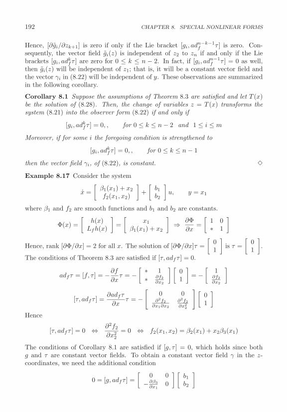
192 CHAPTER 8. SPECIAL NONLINEAR FORMS
Hence, [∂gi/∂zk+1] is zero if only if the Lie bracket [gi, adn−k−1f τ ] is zero. Con-
sequently, the vector field gi(z) is independent of z2 to zn if and only if the Liebrackets [gi, adk
fτ ] are zero for 0 ≤ k ≤ n − 2. In fact, if [gi, adn−1f τ ] = 0 as well,
then gi(z) will be independent of z1; that is, it will be a constant vector field andthe vector γi in (8.22) will be independent of y. These observations are summarizedin the following corollary.
Corollary 8.1 Suppose the assumptions of Theorem 8.3 are satisfied and let T (x)be the solution of (8.28). Then, the change of variables z = T (x) transforms thesystem (8.21) into the observer form (8.22) if and only if
[gi, adkfτ ] = 0, , for 0 ≤ k ≤ n − 2 and 1 ≤ i ≤ m
Moreover, if for some i the foregoing condition is strengthened to
[gi, adkfτ ] = 0, , for 0 ≤ k ≤ n − 1
then the vector field γi, of (8.22), is constant. �
Example 8.17 Consider the system
x =[
β1(x1) + x2
f2(x1, x2)
]+[
b1
b2
]u, y = x1
where β1 and f2 are smooth functions and b1 and b2 are constants.
Φ(x) =[
h(x)Lfh(x)
]=[
x1
β1(x1) + x2
]⇒ ∂Φ
∂x=[
1 0∗ 1
]
Hence, rank [∂Φ/∂x] = 2 for all x. The solution of [∂Φ/∂x]τ =[
01
]is τ =
[01
].
The conditions of Theorem 8.3 are satisfied if [τ, adfτ ] = 0.
adfτ = [f, τ ] = −∂f
∂xτ = −
[ ∗ 1∗ ∂f2
∂x2
] [01
]= −
[1
∂f2∂x2
]
[τ, adfτ ] =∂adfτ
∂xτ = −
[0 0
∂2f2∂x1∂x2
∂2f2∂x2
2
] [01
]Hence
[τ, adfτ ] = 0 ⇔ ∂2f2
∂x22
= 0 ⇔ f2(x1, x2) = β2(x1) + x2β3(x1)
The conditions of Corollary 8.1 are satisfied if [g, τ ] = 0, which holds since bothg and τ are constant vector fields. To obtain a constant vector field γ in the z-coordinates, we need the additional condition
0 = [g, adfτ ] =[
0 0−∂β3
∂x10
] [b1
b2
]
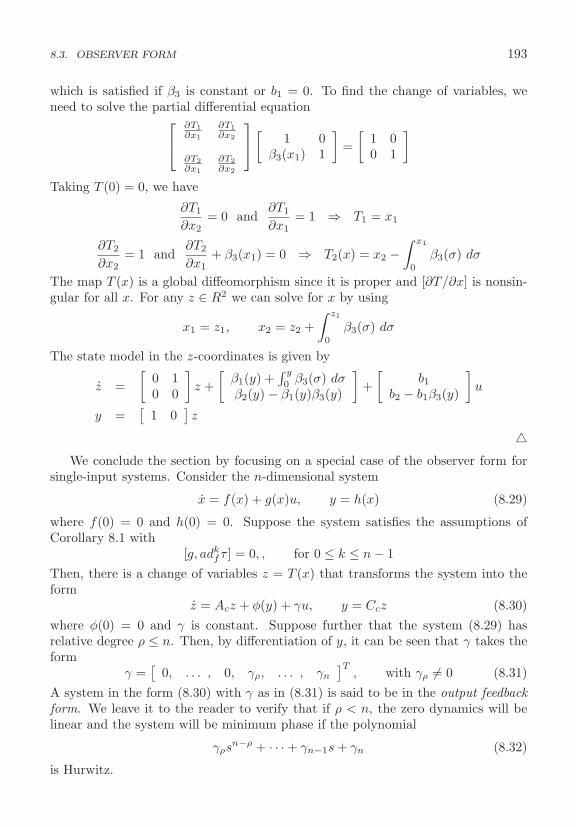
8.3. OBSERVER FORM 193
which is satisfied if β3 is constant or b1 = 0. To find the change of variables, weneed to solve the partial differential equation⎡
⎣ ∂T1∂x1
∂T1∂x2
∂T2∂x1
∂T2∂x2
⎤⎦[ 1 0
β3(x1) 1
]=[
1 00 1
]
Taking T (0) = 0, we have
∂T1
∂x2= 0 and
∂T1
∂x1= 1 ⇒ T1 = x1
∂T2
∂x2= 1 and
∂T2
∂x1+ β3(x1) = 0 ⇒ T2(x) = x2 −
∫ x1
0
β3(σ) dσ
The map T (x) is a global diffeomorphism since it is proper and [∂T/∂x] is nonsin-gular for all x. For any z ∈ R2 we can solve for x by using
x1 = z1, x2 = z2 +∫ z1
0
β3(σ) dσ
The state model in the z-coordinates is given by
z =[
0 10 0
]z +[
β1(y) +∫ y
0β3(σ) dσ
β2(y) − β1(y)β3(y)
]+[
b1
b2 − b1β3(y)
]u
y =[
1 0]z
�We conclude the section by focusing on a special case of the observer form for
single-input systems. Consider the n-dimensional system
x = f(x) + g(x)u, y = h(x) (8.29)
where f(0) = 0 and h(0) = 0. Suppose the system satisfies the assumptions ofCorollary 8.1 with
[g, adkfτ ] = 0, , for 0 ≤ k ≤ n − 1
Then, there is a change of variables z = T (x) that transforms the system into theform
z = Acz + φ(y) + γu, y = Ccz (8.30)where φ(0) = 0 and γ is constant. Suppose further that the system (8.29) hasrelative degree ρ ≤ n. Then, by differentiation of y, it can be seen that γ takes theform
γ =[
0, . . . , 0, γρ, . . . , γn
]T, with γρ = 0 (8.31)
A system in the form (8.30) with γ as in (8.31) is said to be in the output feedbackform. We leave it to the reader to verify that if ρ < n, the zero dynamics will belinear and the system will be minimum phase if the polynomial
γρsn−ρ + · · · + γn−1s + γn (8.32)
is Hurwitz.
194 CHAPTER 8. SPECIAL NONLINEAR FORMS
8.4 Exercises
8.1 For each of the following systems,
(a) Find the relative degree and show that the system is minimum phase.
(b) Transform the system into the normal form. Is the change of variables validglobally?
(c) Under what additional conditions is the system feedback linearizable?
(d) Under the conditions of part (c), find a change of variables that transformsthe system into the controller form. Under what additional conditions is thechange of variables a global diffeomorphism?
(1) x1 = x2, x2 = −ϕ(x1) − x2 + u, y = x1 + 2x2, where ϕ(0) = 0, x1ϕ(x1) ≥β1x
21 ∀ x1, and β1 > 0.
(2) x1 = −x1 − x2 + u, x2 = ϕ1(x1) − ϕ2(x2), y = x1 + x2, where ϕ1 and ϕ2
belong to the sectors [αi, βi] with βi > αi > 0, for i = 1, 2.
(3) x1 = −ϕ1(x1)+ϕ2(x2), x2 = −x1−x2 +x3, x3 = −x3 +u, y = x2, whereϕ1 and ϕ2 are smooth and belong to the sectors [αi, βi] with βi > αi > 0, fori = 1, 2.
8.2 For each of the following systems, find the relative degree and determine if thesystem is minimum phase.
(1) The boost converter (A.16) when the output is x1.
(2) The boost converter (A.16) when the output is x2.
(3) The biochemical reactor (A.19), with (A.20), when the output is y = x1 − 1.
(4) The biochemical reactor (A.19), with (A.20), when the output is y = x2 − 1.
(5) The magnetic levitation system (A.30)–(A.32) when the output is x1.
(6) The electrostatic microactuator (A.33) when the output is x1
(7) The electrostatic microactuator (A.33) when the output is x3
(8) The inverted pendulum on a cart (A.41)–(A.44) when the output is x1.
(9) The inverted pendulum on a cart (A.41)–(A.44) when the output is x3.
(10) The TORA system (A.49)–(A.52) when the output is x1.
(11) The TORA system (A.49)–(A.52) when the output is x3.
8.4. EXERCISES 195
8.3 For each of the following systems investigate whether the system is feedbacklinearizable. If it is so, find a change of variables that transforms the system in thecontroller form and determine its domain of validity.
(1) The boost converter (A.16).
(2) The biochemical reactor (A.19) with ν defined by (A.20).
(3) The magnetic levitation system (A.30)–(A.32).
(4) The electrostatic microactuator (A.33).
(5) The inverted pendulum (A.47).
8.4 Consider the field-controlled DC motor (A.25) with δ = 0.
(a) Show that neglecting the armature circuit dynamics by setting Ta = 0 resultsin the two-dimensional model
x1 = a1[−fe(x1) + u], x2 = a2[x1(Va − x1x2) − f�(x2)]
where x2 and x3 of (A.25) are renamed x1 and x2, respectively.
(b) Study the relative degree when y = x2.
(c) Study feedback linearization.
8.5 Consider the system
x1 = x1 +x2
1 + x21
, x2 = −x2 + x3, x3 = x1x2 + u
(a) If the output is x2, find the relative degree of the system and determine if it isminimum phase.
(b) Repeat (a) if the output is x1.
(c) Show that the system is feedback linearizable.
(d) Find a change of variables that transforms the system into the controller formand determine its domain of validity.
8.6 A semitrailer-like vehicle can be modeled by the state equation
x1 = tan(x3)
x2 = − tan(x2)a cos(x3)
+1
b cos(x2) cos(x3)tan(u)
x3 =tan(x2)a cos(x3)
where a and b are positive constants. Restrict u to Du = {|u| < π/2} and x toDx = {|x2| < π/2, |x3| < π/2}. Then, cos(x2) = 0, cos(x3) = 0, and tan(u) isinvertible.

196 CHAPTER 8. SPECIAL NONLINEAR FORMS
(a) Show that the change of variables w = tan(u)/(b cos(x2) cos(x3)) transformsthe system into the form
x = f(x) + gw, where f =
⎡⎣ tan(x3)
− tan(x2)/(a cos(x3))tan(x2)/(a cos(x3))
⎤⎦ , g =
⎡⎣ 0
10
⎤⎦
(b) Show that the system is feedback linearizable.
(c) Find a change of variables that transforms the system into the controller formand determine its domain of validity.
8.7 Show that the electrostatic microactuator (A.33) with output y = col(x1, x3).is in the observer form.
8.8 For each of the following systems, determine if the system is transformable intothe observer form. If yes, find the change of variables and determine its domain ofvalidity.
(1) x1 = x2, x2 = −3x21x2 − x1 − x3
1 − x2 + u, y = x1.
(2) x1 = x2, x2 = −x22 + x3, x3 = x2
1 − 2x32 + 2x2x3 + u, y = x1
(3) The van der Pol equation: x1 = x2, x2 = −x1 + x2 − 13x3
2 + u, y = x1
(4)
x1 = β1(x1) + x2 + b1u
x2 = β2(x1) + β3(x1)x2 + x3 + b2u
x3 = β4(x1) + β5(x1)x2 + ax3 + b3u
y = x1
The functions β1 to β5 are smooth.
8.9 Consider an n-dimensional system of the form (8.30), which has relative degreeρ < n. Show that the vector γ takes the form (8.31) and the system is minimumphase if the polynomial (8.32) is Hurwitz.
Chapter 9
State Feedback Stabilization
Stabilization of equilibrium points is the core task in feedback control of nonlinearsystems. The problem is important in its own sake and is at the heart of othercontrol problems such as tracking and regulation. Stabilization is treated in threechapters, starting with state feedback stabilization in this chapter, followed by ro-bust stabilization in Chapter 10, and output feedback stabilization in Chapter 12.1
9.1 Basic Concepts
The state feedback stabilization problem for the system
x = f(x, u)
is to design a feedback controller u = φ(x) such that the origin x = 0 is an asymp-totically stable equilibrium point of the closed-loop system
x = f(x, φ(x))
The control u = φ(x) is usually called “static feedback” because it is a memorylessfunction of x. We may use a dynamic state feedback controller u = φ(x, z) where zis the state of a dynamic system of the form
z = g(x, z)
In this case the origin to be stabilized is (x = 0, z = 0). Examples of dynamic statefeedback control arise when we use integral or adaptive control.
While the standard problem is defined as stabilization of an equilibrium pointat the origin, we can use the same formulation to stabilize the system with respect
1For further reading on stabilization, see [8, 19, 31, 32, 33, 36, 40, 43, 66, 67, 71, 75, 80, 81, 86,91, 107, 115, 121, 137, 141].
197
198 CHAPTER 9. STATE FEEDBACK STABILIZATION
to an arbitrary point xss. For that we need the existence of a steady-state controluss that can maintain equilibrium at xss; namely,
0 = f(xss, uss)
The change of variables
xδ = x − xss, uδ = u − uss
results inxδ = f(xss + xδ, uss + uδ)
def= fδ(xδ, uδ)
where fδ(0, 0) = 0. We can now proceed to the solve the standard stabilizationproblem for the system
xδ = fδ(xδ, uδ)
where uδ is designed as feedback control of xδ. The overall control u = uδ +uss hasa feedback component uδ and a feedforward component uss.
When a linear system is stabilized by linear feedback, the origin of the closed-loop system is globally asymptotically stable. This is not the case for nonlinearsystems where different stabilization notions can be introduced. If the feedbackcontrol guarantees asymptotic stability of the origin but does not prescribe a re-gion of attraction, we say that the feedback control achieves local stabilization. If itguarantees that a certain set is included in the region of attraction or an estimateof the region of attraction is given, we say that the feedback control achieves re-gional stabilization. Global stabilization is achieved if the origin of the closed-loopsystem is globally asymptotically stable. If feedback control does not achieve globalstabilization, but can be designed such that any given compact set (no matter howlarge) can be included in the region of attraction, we say that the feedback controlachieves semiglobal stabilization. It is typical in this case that the feedback controldepends on parameters that can be adjusted to enlarge the region of attraction.These four stabilization notions are illustrated by the next example.
Example 9.1 Suppose we want to stabilize the scalar system
x = x2 + u
by state feedback. Linearization at the origin results in the linear system x = u,which can be stabilized by u = −kx with k > 0. When this control is applied tothe nonlinear system, it results in
x = −kx + x2
whose linearization at the origin is x = −kx. Thus, by Theorem 3.2, the originis asymptotically stable, and we say that u = −kx achieves local stabilization. Inthis example, it is not hard to see that the region of attraction is the set {x < k}.With this information, we say that u = −kx achieves regional stabilization. By

9.2. LINEARIZATION 199
increasing k, we can expand the region of attraction. In fact, any compact set ofthe form {−a ≤ x ≤ b}, with positive a and b, can be included it in the region ofattraction by choosing k > b. Hence, u = −kx achieves semiglobal stabilization. Itis important to notice that u = −kx does not achieve global stabilization. In fact,for any finite k, there is a part of the state space (that is, x ≥ k), which is not inthe region of attraction. While semiglobal stabilization can include any compactset in the region of attraction, the controller is dependent on the given set and willnot necessarily work with a bigger set. For a given b, we can choose k > b. Once kis fixed and the controller is implemented, if the initial state happens to be in theregion {x > k}, the solution x(t) will diverge to infinity. Global stabilization can beachieved by the nonlinear controller u = −x2 − kx, which cancels the nonlinearityand yields the closed-loop system x = −kx. �
9.2 Linearization
The stabilization problem is well understood for the linear system
x = Ax + Bu
where the state feedback control u = −Kx preserves linearity of the open-loopsystem, and the origin of the closed-loop system
x = (A − BK)x
is asymptotically stable if and only if the matrix A − BK is Hurwitz. Thus, thestate feedback stabilization problem reduces to a problem of designing a matrix K toassign the eigenvalues of A−BK in the open left-half complex plane. Linear controltheory2 confirms that the eigenvalues of A−BK can be arbitrarily assigned (subjectonly to the constraint that complex eigenvalues are in conjugate pairs) providedthe pair (A,B) is controllable. Even if some eigenvalues of A are not controllable,stabilization is still possible if the uncontrollable eigenvalues have negative realparts. In this case, the pair (A,B) is called stabilizable, and the uncontrollable(open-loop) eigenvalues of A will be (closed-loop) eigenvalues of A − BK.
For nonlinear systems, the problem is more difficult and less understood. Asimple approach is to use linearization. Consider the system
x = f(x, u) (9.1)
where f(0, 0) = 0 and f(x, u) is continuously differentiable in a domain Dx × Du
of Rn × Rm containing the origin (x = 0, u = 0). We want to design a statefeedback controller u = φ(x) to stabilize the system. Linearization of (9.1) about(x = 0, u = 0) results in the linear system
x = Ax + Bu (9.2)2See, for example, [2], [22], [59], [82], or [114].
200 CHAPTER 9. STATE FEEDBACK STABILIZATION
where
A =∂f
∂x(x, u)
∣∣∣∣x=0,u=0
; B =∂f
∂u(x, u)
∣∣∣∣x=0,u=0
Assume the pair (A,B) is controllable, or at least stabilizable. Design a matrix K toassign the eigenvalues of A−BK to desired locations in the open left-half complexplane. Now apply the linear state feedback control u = −Kx to the nonlinearsystem (9.1) to obtain the closed-loop system
x = f(x,−Kx) (9.3)
Clearly, the origin x = 0 is an equilibrium point of the closed-loop system. Thelinearization of (9.3) about the origin is given by
x =[∂f
∂x(x,−Kx) +
∂f
∂u(x,−Kx) (−K)
]x=0
x = (A − BK)x
Since A − BK is Hurwitz, it follows from Theorem 3.2 that the origin is an ex-ponentially stable equilibrium point of the closed-loop system (9.3). Moreover, wecan find a quadratic Lyapunov function for the closed-loop system. Let Q be anypositive-definite symmetric matrix and solve the Lyapunov equation
P (A − BK) + (A − BK)T P = −Q
for P . Since (A − BK) is Hurwitz, the Lyapunov equation has a unique positivedefinite solution (Theorem 3.7). The quadratic function V (x) = xT Px is a Lya-punov function for the closed-loop system in the neighborhood of the origin. Wecan use V (x) to estimate the region of attraction.
Example 9.2 Consider the pendulum equation (A.1):
θ + sin θ + bθ = cu
Suppose we want to design u to stabilize the pendulum at an angle θ = δ1. Forthe pendulum to maintain equilibrium at θ = δ1, the steady-state control uss mustsatisfy
sin δ1 = cuss
Choose the state variables as x1 = θ − δ1, x2 = θ and set uδ = u − uss. The stateequation
x1 = x2, x2 = −[sin(x1 + δ1) − sin δ1] − bx2 + cuδ
is in the standard form (9.1), where f(0, 0) = 0. Linearization at the origin yields
A =[
0 1− cos(x1 + δ1) −b
]x1=0
=[
0 1− cos δ1 −b
]; B =
[0c
]
9.3. FEEDBACK LINEARIZATION 201
The pair (A,B) is controllable. Taking K = [k1 k2], it can be verified that A−BKis Hurwitz for
k1 > − cos δ1
c, k2 > − b
cThe control u is given by
u =sin δ1
c− Kx =
sin δ1
c− k1(θ − δ1) − k2θ
�
9.3 Feedback Linearization
Consider the nonlinear system
x = f(x) + G(x)u
where f(0) = 0, x ∈ Rn, and u ∈ Rm. Let D be a domain of Rn containing theorigin and suppose there is a diffeomorphism T (x) on D, with T (0) = 0, such thatthe change of variables z = T (x) transforms the system into the controller form
z = Az + B[ψ(x) + γ(x)u]
where (A,B) is controllable and γ(x) is a nonsingular matrix for all x ∈ D. Letγ−1(x) be the inverse matrix of γ(x) for each x. The feedback control
u = γ−1(x)[−ψ(x) + v]
cancels the nonlinearity and converts the system into
z = Az + Bv
Hence, the origin z = 0 can be stabilized by v = −Kz, where A − BK is Hurwitz.The closed-loop system, in the z-coordinates, is
z = (A − BK)z
and the origin z = 0 is exponentially stable. In the x-coordinates, the control isgiven by
u = γ−1(x)[−ψ(x) − KT (x)]
and the closed-loop system is
x = f(x) + G(x)γ−1(x)[−ψ(x) − KT (x)] def= fc(x)
The origin in the x-coordinates inherits exponential stability of the origin in thez-coordinates because T (x) is a diffeomorphism in the neighborhood of x = 0. Inparticular, since
z =∂T
∂x(x)x = (A − BK)z
202 CHAPTER 9. STATE FEEDBACK STABILIZATION
we have∂T
∂x(x)fc(x) = (A − BK)T (x)
Calculating the Jacobian matrix of each side of the preceding equation at x = 0and using the fact that fc(0) = 0, we obtain
∂fc
∂x(0) = J−1(A − BK)J, where J =
∂T
∂x(0)
The matrix J is nonsingular and the similarity transformation J−1(A−BK)J pre-serves the eigenvalues of A − BK. Hence, J−1(A − BK)J is Hurwitz and x = 0 isexponentially stable by Theorem 3.2. If D = Rn and T (x) is a global diffeomor-phism, then x = 0 will be globally asymptotically stable. If T (x) is a diffeomor-phism on a domain D ⊂ Rn so that the equation z = (A − BK)z is valid in thedomain T (D), then the region of attraction can be estimated in the z coordinatesby Ωc = {zT Pz ≤ c}, where P = PT > 0 is the solution of the Lyapunov equation
P (A − BK) + (A − BK)T P = −Q, for some Q = QT > 0 (9.4)
and c > 0 is chosen such that Ωc ⊂ T (D). The estimate in the x-coordinates isgiven by T−1(Ωc) = {TT (x)PT (x) ≤ c}.Example 9.3 We saw in Example 8.12 that the system
x1 = a sin x2, x2 = −x21 + u
can be transformed into the controller form by the change of variables
z = T (x) =[
x1
a sin x2
]where T (x) is a diffeomorphism on D = {|x2| < π/2} and T (D) = {|z2| < a}. TakeK =
[σ2 2σ
], with σ > 0, to assign the eigenvalues of A−BK at −σ, −σ. The
Lyapunov equation (9.4) is satisfied with
P =[
3σ2 σσ 1
], Q =
[2σ3 00 2σ
]The region of attraction is estimated by
{3σ2x21 + 2σax1 sin x2 + a2 sin2 x2 ≤ c}
where3
c < min|z2|=a
zT Pz =a2[
0 1]P−1
[01
] =2a2
3
�3See Section 3.6 and equation (B.3).
9.3. FEEDBACK LINEARIZATION 203
Feedback linearization is based on exact mathematical cancellation of the non-linear terms γ and ψ, which requires knowledge of γ, ψ, and T . This is almostimpossible for several practical reasons such as model simplification, parameter un-certainty, and computational errors. Most likely, the controller will be implementingfunctions γ, ψ, and T , which are approximations of γ, ψ, and T ; that is to say, theactual control will be
u = γ−1(x)[−ψ(x) − KT (x)]
The closed-loop system under this feedback control is given by
z = Az + B{ψ(x) + γ(x)γ−1(x)[−ψ(x) − KT (x)]}By adding and subtracting the term BKz to the right-hand side we can rewrite theclosed-loop system as
z = (A − BK)z + BΔ(z) (9.5)
where
Δ(z) ={
ψ(x) + γ(x)γ−1(x)[−ψ(x) − KT (x)] + KT (x)}
x=T−1(z)
The system (9.5) is a perturbation of the nominal system z = (A − BK)z. Theeffect of the perturbation term BΔ(z) can be investigated by using the techniquesof Section 4.2 when Δ(0) = 0 and those of Section 4.3 when Δ(0) = 0. The nextlemma summarizes the results of such investigation.
Lemma 9.1 Suppose the closed-loop system (9.5) is well defined in a domain Dz ⊂Rn containing the origin, and ‖Δ(z)‖ ≤ k‖z‖ for all z ∈ Dz. Let P be the solutionof the Lyapunov equation (9.4) with Q = I. Then, the origin z = 0 is exponentiallystable if
k <1
2‖PB‖ (9.6)
If Dz = Rn, the origin will be globally exponentially stable. Furthermore, suppose‖Δ(z)‖ ≤ k‖z‖+δ for all z ∈ Dz, where k satisfies (9.6) and δ > 0. Take r > 0 suchthat Br ⊂ Dz. Then there exist positive constants c1 and c2 such that if δ < c1r andz(0) ∈ {zT Pz ≤ λmin(P )r2}, ‖z(t)‖ will be ultimately bounded by δc2. If Dz = Rn,‖z(t)‖ will be globally ultimately bounded by δc2 for any δ > 0.
Proof: With V (z) = zT Pz, we have
V = zT [P (A − BK) + (A − BK)T P ]z + 2zT PBΔ(z)≤ −‖z‖2 + 2‖PB‖ ‖z‖ ‖Δ(z)‖
If ‖Δ(z)‖ ≤ k‖z‖ + δ, then
V ≤ −‖z‖2 + 2k‖PB‖ ‖z‖2 + 2δ‖PB‖ ‖z‖= −(1 − θ1)‖z‖2 − θ1‖z‖2 + 2k‖PB‖ ‖z‖2 + 2δ‖PB‖ ‖z‖
204 CHAPTER 9. STATE FEEDBACK STABILIZATION
where θ1 ∈ (0, 1) is chosen close enough to one such that k < θ1/(2‖PB‖). Conse-quently,
V ≤ −(1 − θ1)‖z‖2 + 2δ‖PB‖ ‖z‖If ‖Δ(z)‖ ≤ k‖z‖, we set δ = 0 in the preceding inequality and conclude that theorigin z = 0 is exponentially stable, or globally exponentially stable if Dz = Rn. Ifδ > 0,
V ≤ −(1 − θ1)(1 − θ2)‖z‖2, ∀ ‖z‖ ≥ 2δ‖PB‖(1 − θ1)θ2
def= δc0
where θ2 ∈ (0, 1). Theorem 4.5 shows that if δc0 < r√
λmin(P )/λmax(P ) and z(0) ∈{zT Pz ≤ λmin(P )r2}, then ‖z(t)‖ is ultimately bounded by δc0
√λmax(P )/λmin(P ).
If Dz = Rn, the constant r can be chosen arbitrarily large; hence the ultimate boundholds for any initial state z(0) with no restriction on how large δc0 is. �
Example 9.4 Consider the pendulum equation
x1 = x2, x2 = − sin(x1 + δ1) − bx2 + cu
from Example 9.2. A linearizing-stabilizing feedback control is given by
u =(
1c
)[sin(x1 + δ1) − (k1x1 + k2x2)]
where k1 and k2 are chosen such that
A − BK =[
0 1−k1 −(k2 + b)
]
is Hurwitz. Suppose, due to uncertainties in the parameter c, the actual control is
u =(
1c
)[sin(x1 + δ1) − (k1x1 + k2x2)]
where c is an estimate of c. The closed-loop system is given by
x1 = x2, x2 = −k1x1 − (k2 + b)x2 + Δ(x)
where
Δ(x) =(
c − c
c
)[sin(x1 + δ1) − (k1x1 + k2x2)]
The error term Δ(x) satisfies the bound |Δ(x)| ≤ k‖x‖ + δ globally with
k =∣∣∣∣c − c
c
∣∣∣∣(
1 +√
k21 + k2
2
), δ =
∣∣∣∣c − c
c
∣∣∣∣ | sin δ1|
9.3. FEEDBACK LINEARIZATION 205
The constants k and δ are measures of the size of the error in estimating c. Let Pbe the solution of the Lyapunov equation P (A − BK) + (A − BK)T P = −I. If
k <1
2√
p212 + p2
22
, where P =[
p11 p12
p12 p22
]
then the solutions are globally ultimately bounded and the ultimate bound is pro-portional to δ. If sin δ1 = 0, the foregoing bound on k ensures global exponentialstability of the origin. Satisfying the foregoing inequality is not a problem when theuncertainty is sufficiently small, but for large uncertainty it constraints the choice ofK; it might even be impossible to choose K for which the inequality is satisfied. Toillustrate this point let us neglect friction by setting b = 0 and consider uncertaintyin the mass m. Then, c = mo/m, where m is an estimate of m. The constants kand δ are given by
k = Δm
[1 +√
k21 + k2
2
], δ = Δm| sin δ1|, where Δm =
∣∣∣∣m − m
m
∣∣∣∣Let K =
[σ2 2σ
]to assign eigenvalues of A − BK at −σ and −σ for a positive
σ. By solving the Lyapunov equation (9.4) with Q = I, it can be verified that theinequality k < 1/(2
√p212 + p2
22) is equivalent to
Δm <2σ3
[1 + σ√
σ2 + 4]√
4σ2 + (σ2 + 1)2
By plotting the right-hand side as a function of σ it can be seen that it increasesmonotonically with σ until it reaches a maximum value of 0.3951, after which itdecreases monotonically towards zero. Hence, the inequality cannot be satisfied ifΔm > 0.3951 and for every value of Δm less than 0.3951, the inequality is satisfiedfor a range of values of σ. For example, for Δm = 0.3, σ should be restricted to1.37 < σ < 5.57. �
The foregoing Lyapunov analysis shows that the stabilizing component of thefeedback control u = γ−1(x)[−ψ(x)−KT (x)] achieves a certain degree of robustnessto model uncertainty. We will see in Chapter 10 that the stabilizing component canbe designed to achieve a higher degree of robustness by exploiting the fact that theperturbation term BΔ(z) in (9.5) belongs to the range space of the input matrix B.Such perturbation is said to satisfy the matching condition. The techniques of theChapter 10 can guarantee robustness to arbitrarily large Δ(z) provided an upperbound on ‖Δ(z)‖ is known.
The basic philosophy of feedback linearization is to cancel the nonlinear termsof the system. Aside from the issues of whether or not we can cancel the nonlinearterms, effect of uncertainties, implementation factors, and so on, we should examinethe philosophy itself: Is it a good idea to cancel nonlinear terms? Our motivation to

206 CHAPTER 9. STATE FEEDBACK STABILIZATION
do so has been mathematically driven. We wanted to linearize the system to makeit more tractable and use the relatively well-developed linear control theory. Froma performance viewpoint, however, a nonlinear term could be “good” or “bad” andthe decision whether we should use feedback to cancel a nonlinear term is, in reality,problem dependent. Let us use a couple of examples to illustrate this point.
Example 9.5 Consider the scalar system4
x = ax − bx3 + u
where a and b are positive constants. The feedback control
u = −(k + a)x + bx3, k > 0
cancels the nonlinear term −bx3 and results in the closed-loop system x = −kx.But, −bx3 provides “nonlinear damping” and even without any feedback controlit would guarantee boundedness of the solution despite the fact that the origin isunstable. So, why should we cancel it? If we simply use the linear control
u = −(k + a)x, k > 0
we will obtain the closed-loop system x = −kx− bx3 whose origin is globally expo-nentially stable and its trajectories approach the origin faster than the trajectoriesof x = −kx. Moreover, the linear control uses less control effort and is simpler toimplement. �Example 9.6 Consider the two-dimensional system
x1 = x2, x2 = −h(x1) + u
where h(0) = 0 and x1h(x1) > 0 for all x1 = 0. The system is feedback linearizableand a linearizing–stabilizing feedback control can be taken as
u = h(x1) − (k1x1 + k2x2)
where k1 and k2 are chosen to assign the closed-loop eigenvalues at desired locationsin the left-half complex plane. On the other hand, with y = x2 as the output, thesystem is passive with the positive definite storage function V =
∫ x1
0h(z) dz + 1
2x22.
In particular, V = yu. The feedback control
u = −σ(x2)
where σ is any locally Lipschitz function that satisfies σ(0) = 0 and yσ(y) > 0 fory = 0, results in
V = −x2σ(x2) ≤ 04The example is taken from [42].
9.4. PARTIAL FEEDBACK LINEARIZATION 207
Becausex2(t) ≡ 0 ⇒ x2(t) ≡ 0 ⇒ h(x1(t)) ≡ 0 ⇒ x1(t) ≡ 0
asymptotic stability of the origin follows from the invariance principle. The controlu = −σ(x2) has two advantages over the linearizing feedback control. First, it doesnot use a model of the nonlinear function h. Hence, it is robust to uncertainty inmodeling h. Second, the flexibility in choosing the function σ can be used to reducethe control effort. For example, we can meet any constraint of the form |u| ≤ k,by choosing u = −k sat(x2). However, the control u = −σ(x2) cannot arbitrarilyassign the rate of decay of x(t). Linearization of the closed-loop system at the originyields the characteristic equation
s2 + σ′(0)s + h′(0) = 0
One of the two roots of the foregoing equation cannot be moved to the left ofRe[s] = −√h′(0). Feedback controllers that exploit passivity will be discussed inSection 9.6. �
These two examples make the point that there are situations where nonlinearitiesare beneficial and cancelling them should not be an automatic choice. We shouldtry our best to understand the effect of the nonlinear terms and decide whether ornot cancellation is appropriate. Admittedly, this is not an easy task.
9.4 Partial Feedback Linearization
Consider the nonlinear system
x = f(x) + G(x)u
where f(0) = 0, x ∈ Rn, and u ∈ Rm. Let D be a domain of Rn containing theorigin and suppose there is a diffeomorphism T (x) on D, with T (0) = 0, such thatthe change of variables
z =[
ηξ
]= T (x) =
[T1(x)T2(x)
]transforms the system into the form
η = f0(η, ξ), ξ = Aξ + B[ψ(x) + γ(x)u] (9.7)
where ξ ∈ Rρ, η ∈ Rn−ρ, (A,B) is controllable, and γ(x) is a nonsingular matrixfor all x ∈ D. It follows from the preceding assumptions that f0(0, 0) = 0 andψ(0) = 0. We assume that f0, ψ, and γ are locally Lipschitz. Our goal is to designstate feedback control to stabilize the origin. The form (9.7) is motivated by thenormal form of Section 8.1, but the output equation is dropped since it plays no

208 CHAPTER 9. STATE FEEDBACK STABILIZATION
role in state feedback stabilization. We do not restrict our discussion in this sectionto single-input systems or to a pair (A,B) in the controllable canonical form.
The state feedback control
u = γ−1(x)[−ψ(x) + v]
reduces (9.7) toη = f0(η, ξ), ξ = Aξ + Bv (9.8)
Equation ξ = Aξ + Bv can be stabilized by v = −Kξ, where (A−BK) is Hurwitz.The closed-loop system
η = f0(η, ξ), ξ = (A − BK)ξ (9.9)
is a cascade connection of the system η = f0(η, ξ) with the linear system ξ =(A − BK)ξ. It is clear that asymptotic stability of the origin of η = f0(η, 0) is anecessary condition for asymptotic stability of the origin of the cascade connectionbecause with the initial state ξ(0) = 0 we have ξ(t) ≡ 0 and the trajectories of thecascade connection coincide with those of η = f0(η, 0). The next lemma shows thatthis condition is sufficient as well.
Lemma 9.2 The origin of the cascade connection (9.9) is asymptotically (respec-tively, exponentially) stable if the origin of η = f0(η, 0) is asymptotically (respec-tively, exponentially) stable. �
The lemma is proved by constructing composite Lyapunov functions as in Sec-tion C.1. In the case of asymptotic stability, the Lyapunov function is bV1(η) +√
ξT Pξ, with sufficiently small b > 0, where V1(η) is provided by (the converseLyapunov) Theorem 3.9 and P = PT > 0 is the solution of the Lyapunov equationP (A−BK)+(A−BK)T P = −I. In the case of exponential stability, the Lyapunovfunction is bV1(η) + ξT Pξ, with sufficiently small b > 0, where V1(η) is provided by(the converse Lyapunov) Theorem 3.8.
Lemma 9.2 shows that a minimum phase, input–output linearizable, single-input–single-output system can be stabilized by the state feedback control
u = γ−1(x)[−ψ(x) − KT2(x)] (9.10)
which is independent of T1(x). Therefore, it is independent of the function φ thatsatisfies the partial differential equation (7.8).
Lemma 9.2 is a local result. The next two examples show that global asymptoticstability of the origin of η = f0(η, ξ) is not sufficient for global asymptotic stabilityof the origin of the cascade connection.

9.4. PARTIAL FEEDBACK LINEARIZATION 209
Example 9.7 Consider the two-dimensional system5
η = −η + η2ξ, ξ = v
The origin of η = −η is globally exponentially stable. With v = −kξ, k > 0, we cansee by linearization that the origin (η, ξ) = (0, 0) of the full system is exponentiallystable. However, it is not globally asymptotically stable. This fact can be seen asfollows. Taking ν = ηξ and noting that
ν = ηξ + ηξ = −kηξ − ηξ + η2ξ2 = −(1 + k)ν + ν2
we see that the set {ηξ < 1 + k} is positively invariant. The boundary ηξ = 1 + k,is a trajectory of the system where η(t) = (1 + k)ekt and ξ(t) = e−kt. Inside{ηξ < 1 + k}, ν(t) will be strictly decreasing and after a finite time T , ν(t) ≤ 1
2for all t ≥ T . Then, ηη ≤ − 1
2η2, for all t ≥ T , which shows that the trajectoryapproaches the origin as t tends to infinity. Hence, {ηξ < 1 + k} is the region ofattraction. While the origin is not globally asymptotically stable, we can includeany compact set in the region of attraction by choosing k large enough. Thus,v = −kξ can achieve semiglobal stabilization. �
If the origin of η = f0(η, 0) is globally asymptotically stable, one might thinkthat the system (9.8) can be globally stabilized, or at least semiglobally stabilized,by designing the linear feedback control v = −Kξ to assign the eigenvalues of(A−BK) far to the left in the complex plane so that the solution of ξ = (A−BK)ξdecays to zero arbitrarily fast. Then, the solution of ξ = f0(η, ξ) will quicklyapproach the solution of η = f0(η, 0), which is well behaved because its origin isglobally asymptotically stable. It may even appear that this strategy was used inthe preceding example. The next example shows why such strategy may fail.
Example 9.8 Consider the three-dimensional system6
η = − 12 (1 + ξ2)η3, ξ1 = ξ2, ξ2 = v
The linear feedback control
v = −k2ξ1 − 2kξ2def= −Kξ
assigns the eigenvalues of
A − BK =[
0 1−k2 −2k
]at −k and −k. The exponential matrix
e(A−BK)t =
⎡⎣ (1 + kt)e−kt te−kt
−k2te−kt (1 − kt)e−kt
⎤⎦
5The example is taken from [19].6The example is taken from [137].

210 CHAPTER 9. STATE FEEDBACK STABILIZATION
shows that as k → ∞, the solution ξ(t) will decay to zero arbitrarily fast. Notice,however, that the coefficient of the (2,1) element of the exponential matrix is aquadratic function of k. It can be shown that the absolute value of this elementreaches a maximum value k/e at t = 1/k. While this term can be made to decay tozero arbitrarily fast by choosing k large, its transient behavior exhibits a peak of theorder of k. This phenomenon is known as the peaking phenomenon.7 The interactionof peaking with nonlinear functions could destabilize the system. In particular, forthe initial states η(0) = η0, ξ1(0) = 1, and ξ2(0) = 0, we have ξ2(t) = −k2te−kt and
η = − 12
(1 − k2te−kt
)η3
During the peaking period, the coefficient of η3 is positive, causing |η(t)| to grow.Eventually, the coefficient of η3 will become negative, but that might not happensoon enough to prevent a finite escape time. Indeed, the solution
η2(t) =η20
1 + η20 [t + (1 + kt)e−kt − 1]
shows that if η20 > 1, the system will have a finite escape time if k is chosen large
enough. �A sufficient condition for global asymptotic stability is given in the next lemma,
which follows from Lemma 4.6.
Lemma 9.3 The origin of the cascade connection (9.9) is globally asymptoticallystable if the system η = f0(η, ξ) is input-to-state stable �
In the previous section we studied the effect of uncertainty on feedback lineariza-tion. A similar study is now performed for partial feedback linearization. Assumingthat the implemented control is
u = γ−1(x)[−ψ(x) − KT2(x)]
where γ, ψ, and T2 are approximations of γ, ψ, and T2, respectively, the closed-loopsystem is represented by
η = f0(η, ξ), ξ = (A − BK)ξ + BΔ(z) (9.11)
where
Δ(z) ={
ψ(x) + γ(x)γ−1(x)[−ψ(x) − KT2(x)] + KT2(x)}
x=T−1(z)
The system (9.11) is a cascade connection of η = f0(η, ξ), with ξ as input, andξ = (A−BK)ξ+BΔ, with Δ as input. It follows from Lemma 4.6 that if η = f0(η, ξ)is input-to-state stable, so is the system (9.11), with Δ as input. This observationproves the following lemma.
7To read more about the peaking phenomenon, see [137]. For illustration of the peakingphenomenon in high-gain observers, see Section 11.4.
9.5. BACKSTEPPING 211
Lemma 9.4 Consider the system (9.11) where η = f0(η, ξ) is input-to-state stableand ‖Δ(z)‖ ≤ δ for all z, for some δ > 0. Then, ‖z(t)‖ is globally ultimatelybounded by a class K function of δ. �
The bound ‖Δ(z)‖ ≤ δ could be conservative if Δ(z), or a component of it,vanishes at z = 0. By viewing (9.11) as a perturbation of the nominal system (9.9)and using the analysis of Sections 4.2 and 4.3, we arrive at the following lemma,whose proof is given in Appendix D.
Lemma 9.5 Suppose the origin of η = f0(η, 0) is exponentially stable, the closed-loop system (9.11) is well defined in a domain Dz ⊂ Rn containing the origin, and‖Δ(z)‖ ≤ k‖z‖+ δ for all z ∈ Dz for some positive constants k and δ. Then, thereexist a neighborhood Nz of z = 0 and positive constants k∗, δ∗, and c such that fork < k∗, δ < δ∗, and z(0) ∈ Nz, ‖z(t)‖ will be ultimately bounded by cδ. If δ = 0,the origin of (9.11) will be exponentially stable. �
9.5 Backstepping
Consider the system
η = fa(η) + ga(η)ξ (9.12)ξ = fb(η, ξ) + gb(η, ξ)u (9.13)
where η ∈ Rn and ξ ∈ R are the state variables and u ∈ R is the control input.The functions fa, fb, ga, and gb are smooth8 in a domain that contains the origin(η = 0, ξ = 0). Furthermore, fa(0) = 0. We want to design state feedback controlto stabilize the origin. This system can be viewed as a cascade connection of twosubsystems; the first is (9.12), with ξ as input, and the second (9.13), with u asinput. We start with the system (9.12) and view ξ as the control input. Supposethe system (9.12) can be stabilized by a smooth state feedback control ξ = φ(η),with φ(0) = 0; that is, the origin of
η = fa(η) + ga(η)φ(η)
is asymptotically stable. Suppose further that we know a (smooth, positive definite)Lyapunov function Va(η) that satisfies the inequality
∂Va
∂η[fa(η) + ga(η)φ(η)] ≤ −W (η) (9.14)
where W (η) is positive definite. By adding and subtracting ga(η)φ(η) on the right-hand side of (9.12), we obtain the equivalent representation
η = fa(η) + ga(η)φ(η) + ga(η)[ξ − φ(η)]8We require smoothness of all functions for convenience. It will become clear, however, that in
a particular problem, we only need existence of derivatives up to a certain order.

212 CHAPTER 9. STATE FEEDBACK STABILIZATION
The change of variablesz = ξ − φ(η)
results in the system
η = fa(η) + ga(η)φ(η) + ga(η)zz = F (η, ξ) + gb(η, ξ)u
whereF (η, ξ) = fb(η, ξ) − ∂φ
∂η[fa(η) + ga(η)φ(η) + ga(η)z]
which is similar to the system we started from, except that now the first subsystemhas an asymptotically stable origin when the input z is zero. This feature will beexploited in the design of u to stabilize the overall system. Using
V (η, ξ) = Va(η) + 12z2 = Va(η) + 1
2 [ξ − φ(η)]2 (9.15)
as a Lyapunov function candidate, we obtain
V =∂Va
∂η[fa(η) + ga(η)φ(η)] +
∂Va
∂ηga(η)z + zF (η, ξ) + zgb(η, ξ)u
≤ −W (η) + z
[∂Va
∂ηga(η) + F (η, ξ) + gb(η, ξ)u
]
The first term is negative definite in η. If we can choose u to make the second termnegative definite in z, V will be negative definite in (η, z). This is possible becausegb = 0. In particular, choosing
u = − 1gb(η, ξ)
[∂Va
∂ηga(η) + F (η, ξ) + kz
](9.16)
for some k > 0, yieldsV ≤ −W (η) − kz2
which shows that the origin (η = 0, z = 0) is asymptotically stable. Since φ(0) =0, we conclude that the origin (η = 0, ξ = 0) is asymptotically stable. If allthe assumptions hold globally and Va(η) is radially unbounded, the origin will beglobally asymptotically stable.
Example 9.9 Consider the system
x1 = x21 − x3
1 + x2, x2 = u
which takes the form (9.12)–(9.13) with η = x1 and ξ = x2. We start with thescalar system
x1 = x21 − x3
1 + x2
9.5. BACKSTEPPING 213
with x2 viewed as the control input and proceed to design the feedback controlx2 = φ(x1) to stabilize the origin x1 = 0. With
x2 = −x21 − x1
def= φ(x1) and Va(x1) = 12x2
1
we obtain
x1 = −x1 − x31 and Va = −x2
1 − x41, ∀ x1 ∈ R
Hence, the origin of x1 = −x1 − x31 is globally asymptotically stable. To backstep,
we use the change of variables
z2 = x2 − φ(x1) = x2 + x1 + x21
to transform the system into the form
x1 = −x1 − x31 + z2, z2 = u + (1 + 2x1)(−x1 − x3
1 + z2)
Taking V (x) = 12x2
1 + 12z2
2 as a Lyapunov function candidate for the overall system,we obtain
V = x1(−x1 − x31 + z2) + z2[u + (1 + 2x1)(−x1 − x3
1 + z2)]= −x2
1 − x41 + z2[x1 + (1 + 2x1)(−x1 − x3
1 + z2) + u]
The controlu = −x1 − (1 + 2x1)(−x1 − x3
1 + z2) − z2
yieldsV = −x2
1 − x41 − z2
2
Hence, the origin is globally asymptotically stable. �
The application of backstepping in the preceding example is straightforward dueto the simplicity of scalar designs. For higher-dimensional systems, we may retainthis simplicity via recursive application of backstepping, as illustrated by the nextexample.
Example 9.10 The three-dimensional system
x1 = x21 − x3
1 + x2, x2 = x3, x3 = u
is composed of the two-dimensional system of the previous example with an ad-ditional integrator at the input side. We proceed to apply backstepping as in theprevious example. After one step of backstepping, we know that the system
x1 = x21 − x3
1 + x2, x2 = x3
214 CHAPTER 9. STATE FEEDBACK STABILIZATION
with x3 as input, can be globally stabilized by the control
x3 = −x1 − (1 + 2x1)(x21 − x3
1 + x2) − (x2 + x1 + x21)
def= φ(x1, x2)
andVa(x1, x2) = 1
2x21 + 1
2 (x2 + x1 + x21)
2
is the corresponding Lyapunov function. To backstep, we apply the change ofvariables z3 = x3 − φ(x1, x2) to obtain
x1 = x21 − x3
1 + x2
x2 = φ(x1, x2) + z3
z3 = u − ∂φ
∂x1(x2
1 − x31 + x2) − ∂φ
∂x2(φ + z3)
Using V = Va + 12z2
3 as a Lyapunov function candidate for the three-dimensionalsystem, we obtain
V =∂Va
∂x1(x2
1 − x31 + x2) +
∂Va
∂x2(z3 + φ)
+ z3
[u − ∂φ
∂x1(x2
1 − x31 + x2) − ∂φ
∂x2(z3 + φ)
]= −x2
1 − x41 − (x2 + x1 + x2
1)2
+ z3
[∂Va
∂x2− ∂φ
∂x1(x2
1 − x31 + x2) − ∂φ
∂x2(z3 + φ) + u
]Taking
u = −∂Va
∂x2+
∂φ
∂x1(x2
1 − x31 + x2) +
∂φ
∂x2(z3 + φ) − z3
yieldsV = −x2
1 − x41 − (x2 + x1 + x2
1)2 − z2
3
Hence, the origin is globally asymptotically stable. �By recursive application of backstepping,9 we can stabilize strict-feedback sys-
tems of the form10
x = f0(x) + g0(x)z1
z1 = f1(x, z1) + g1(x, z1)z2
z2 = f2(x, z1, z2) + g2(x, z1, z2)z3
...zk−1 = fk−1(x, z1, . . . , zk−1) + gk−1(x, z1, . . . , zk−1)zk
zk = fk(x, z1, . . . , zk) + gk(x, z1, . . . , zk)u
(9.17)
9More results on backstepping and other recursive design techniques, including their applicationto uncertain systems, are available in [43, 75, 81, 107, 121].
10If you draw a schematic diagram of the system with the integrators stacked from right to leftas x, z1, z2, etc., you will see that the nonlinearities fi and gi in the zi-equation (i = 1, . . . , k)depend only on x, z1, . . . , zi; that is, on the state variables that are “fed back.”
9.5. BACKSTEPPING 215
where x ∈ Rn, z1 to zk are scalars, f0 to fk vanish at the origin, and
gi(x, z1, . . . , zi) = 0 for 1 ≤ i ≤ k
over the domain of interest. The recursive procedure starts with the system
x = f0(x) + g0(x)z1
where z1 is viewed as the control input. We assume that it is possible to findstabilizing state feedback control z1 = φ0(x), with φ0(0) = 0, and a Lyapunovfunction V0(x) such that
∂V0
∂x[f0(x) + g0(x)φ0(x)] ≤ −W (x)
over the domain of interest for some positive definite function W (x). In many appli-cations of backstepping, the variable x is scalar, which simplifies this stabilizationproblem. With φ0(x) and V0(x) in hand, we proceed to apply backstepping in asystematic way. First, we consider the system
x = f0(x) + g0(x)z1
z1 = f1(x, z1) + g1(x, z1)z2
as a special case of (9.12)–(9.13) with
η = x, ξ = z1, u = z2, fa = f0, ga = g0, fb = f1, gb = g1
We use (9.15) and (9.16) to obtain the stabilizing state feedback control and Lya-punov function as
φ1(x, z1) =1g1
[∂φ0
∂x(f0 + g0z1) − ∂V0
∂xg0 − k1(z1 − φ0) − f1
]for some k1 > 0 and
V1(x, z1) = V0(x) + 12 [z1 − φ0(x)]2
Next, we consider the system
x = f0(x) + g0(x)z1
z1 = f1(x, z1) + g1(x, z1)z2
z2 = f2(x, z1, z2) + g2(x, z1, z2)z3
as a special case of (9.12)–(9.13) with
η =[
xz1
], ξ = z2, u = z3, fa =
[f0 + g0z1
f1
], ga =
[0g1
], fb = f2, gb = g2
216 CHAPTER 9. STATE FEEDBACK STABILIZATION
Using (9.15) and (9.16), we obtain the stabilizing state feedback control and Lya-punov function as
φ2(x, z1, z2) =1g2
[∂φ1
∂x(f0 + g0z1) +
∂φ1
∂z1(f1 + g1z2) − ∂V1
∂z1g1 − k2(z2 − φ1) − f2
]for some k2 > 0 and
V2(x, z1, z2) = V1(x, z1) + 12 [z2 − φ2(x, z1)]2
This process is repeated k times to obtain the overall stabilizing state feedbackcontrol u = φk(x, z1, . . . , zk) and Lyapunov function Vk(x, z1, . . . , zk).
Example 9.11 Consider a single-input–single output system in the normal form11
x = f0(x) + g0(x)z1
zi = zi+1, for 1 ≤ i ≤ ρ − 1zρ = ψ(x, z) + γ(x, z)uy = z1
where x ∈ Rn−ρ, z1 to zρ are scalars, and γ(x, z) = 0 for all (x, z). The system is inthe strict feedback form. The origin can be stabilized by recursive backstepping ifwe can find a smooth function φ0(x) and a smooth Lyapunov function V0(x) suchthat
∂V0
∂x[f0(x) + g0(x)φ0(x)] ≤ −W (x)
for some positive definite function W (x). If the system is minimum phase, then theorigin of x = f0(x) is asymptotically stable. In this case, if we know a Lyapunovfunction V0(x) that satisfies
∂V0
∂xf0(x) ≤ −W (x)
for some positive definite function W (x), we can simply take φ0(x) = 0. �Example 9.12 The system
x = −x + x2z, z = u
was considered in Example 9.7, where it was shown that u = −kz, with sufficientlylarge k > 0, can achieve semiglobal stabilization. In this example, we achieve globalstabilization via backstepping.12 Starting with the system x = −x + x2z, it is clearthat z = 0 and V0(x) = 1
2x2 result in
∂V0
∂x(−x) = −x2, ∀ x ∈ R
11This system is a special case of the normal form of Section 8.1 where the x-equation takes theform f0(x) + g0(x)z1, instead of the more general form f0(x, z).
12The reader can verify that the system is not feedback linearizable near the origin.
9.6. PASSIVITY-BASED CONTROL 217
Using V = V0 + 12z2 = 1
2 (x2 + z2), we obtain
V = x(−x + x2z) + zu = −x2 + z(x3 + u)
Thus, u = −x3 − kz, with k > 0, globally stabilizes the origin. �Example 9.13 As a variation from the previous example, consider the system13
x = x2 − xz, z = u
This time, x = x2 − xz cannot be stabilized by z = 0. It is easy, however, to seethat z = x + x2 and V0(x) = 1
2x2 result in
∂V0
∂x[x2 − x(x + x2)] = −x4, ∀ x ∈ R
Using V = V0 + 12 (z − x − x2)2, we obtain
V = x(x2 − xz) + (z − x − x2)[u − (1 + 2x)(x2 − xz)]= −x4 + (z − x − x2)[−x2 + u − (1 + 2x)(x2 − xz)]
The control
u = (1 + 2x)(x2 − xz) + x2 − k(z − x − x2), k > 0
yieldsV = −x4 − k(z − x − x2)2
Hence, the origin is globally asymptotically stable. �
9.6 Passivity-Based Control
In Chapters 5 and 7, we introduced passivity and studied its role in analyzing thestability of feedback connections. The passivity-based control that we are goingto introduce here is a straightforward application of these chapters, but we do notneed their elaborate details.14 It is enough to recall the definitions of passivity andzero-state observability.
We consider the m-input–m-output system
x = f(x, u), y = h(x) (9.18)
where f is locally Lipschitz in (x, u) and h is continuous in x, for all x ∈ Rn andu ∈ Rm. We assume that f(0, 0) = 0, so that the origin x = 0 is an open-loop
13With the output y = z, the system is nonminimum phase, because the origin of the zero-dynamics x = x2 is unstable.
14More results on passivity-based control are available in [121, 143] and extensive applicationsto physical systems are given in [87, 101].

218 CHAPTER 9. STATE FEEDBACK STABILIZATION
equilibrium point, and h(0) = 0. We recall that the system (9.18) is passive if thereexists a continuously differentiable positive semidefinite storage function V (x) suchthat
uT y ≥ V =∂V
∂xf(x, u), ∀ (x, u) ∈ Rn × Rm (9.19)
The system is zero-state observable if no solution of x = f(x, 0) can stay identicallyin the set {h(x) = 0} other than the zero solution x(t) ≡ 0. Throughout thissection we will require the storage function to be positive definite. The basic ideaof passivity-based control is illustrated in the next theorem.
Theorem 9.1 If the system (9.18) is
1. passive with a radially unbounded positive definite storage function, and
2. zero-state observable,
then the origin x = 0 can be globally stabilized by u = −φ(y), where φ is any locallyLipschitz function such that φ(0) = 0 and yT φ(y) > 0 for all y = 0.
Proof: Use the storage function V (x) as a Lyapunov function candidate for theclosed-loop system
x = f(x,−φ(y))
The derivative of V is given by
V =∂V
∂xf(x,−φ(y)) ≤ −yT φ(y) ≤ 0
Hence, V is negative semidefinite and V = 0 if and only if y = 0. By zero-stateobservability,
y(t) ≡ 0 ⇒ u(t) ≡ 0 ⇒ x(t) ≡ 0
Therefore, by the invariance principle, the origin is globally asymptotically stable.�
The intuition behind the theorem becomes clear when we think of the storagefunction as the energy of the system. A passive system has a stable origin. Allthat is needed to stabilize the origin is the injection of damping so that energy willdissipate whenever x(t) is not identically zero. The required damping is injected bythe function φ. There is great freedom in the choice of φ. We can choose it to meetany constraint on the magnitude of u. For example, if u is constrained to |ui| ≤ ki
for 1 ≤ i ≤ m, we can choose φi(y) = ki sat(yi) or φi(y) = (2ki/π) tan−1(yi).The utility of Theorem 9.1 can be increased by transforming nonpassive systems
into passive ones. Consider, for example, a special case of (9.18), where
x = f(x) + G(x)u (9.20)
Suppose a radially unbounded, positive definite, continuously differentiable functionV (x) exists such that
∂V
∂xf(x) ≤ 0, ∀ x

9.6. PASSIVITY-BASED CONTROL 219
Take
y = h(x) def=[∂V
∂xG(x)
]TThen the system with input u and output y is passive. If it is also zero-stateobservable, we can apply Theorem 9.1.
Example 9.14 Consider the system
x1 = x2, x2 = −x31 + u
With V (x) = 14x4
1 + 12x2
2,
V = x31x2 − x2x
31 + x2u = x2u
Set y = x2 and note that, with u = 0, y(t) ≡ 0 implies that x(t) ≡ 0. Thus, allthe conditions of Theorem 9.1 are satisfied and a globally stabilizing state feedbackcontrol can be taken as u = −kx2 or u = −(2k/π) tan−1(x2) with any k > 0. �
Allowing ourselves the freedom to choose the output function is useful, but weare still limited to state equations for which the origin is open-loop stable. We cancover a wider class of systems if we use feedback to achieve passivity. Consideragain the system (9.20). If a feedback control
u = α(x) + β(x)v (9.21)
and an output function h(x) exist such that the system
x = f(x) + G(x)α(x) + G(x)β(x)v, y = h(x) (9.22)
with input v and output y, satisfies the conditions of Theorem 9.1, we can globallystabilize the origin by using v = −φ(y). The use of feedback to convert a nonpassivesystem into a passive one is known as feedback passivation.15
Example 9.15 Note from Appendix A that the nonlinear dynamic equations foran m-link robot take the form
M(q)q + C(q, q)q + Dq + g(q) = u
where the m-dimensional vectors q and u represent generalized coordinates and con-trol, respectively. The inertia matrix M(q) is symmetric and positive definite for allq, M−2C is skew-symmetric for all q and q, where M is the total derivative of M(q)with respect to t, D is symmetric and positive semidefinite, and the gravity term
15For the system (9.20) with output y = h(x), it is shown in [20] that the system islocally feedback equivalent to a passive system with a positive definite storage function ifrank{[∂h/∂x](0)G(0)} = m and the zero dynamics have a stable equilibrium point at the ori-gin with a positive definite Lyapunov function.
220 CHAPTER 9. STATE FEEDBACK STABILIZATION
g(q) = [∂P (q)/∂q]T , where P (q) is the total potential energy. Consider the prob-lem of designing state feedback control to asymptotically regulate q to a constantreference qr. The regulation error e = q − qr satisfies the differential equation
M(q)e + C(q, q)e + De + g(q) = u
The regulation task is achieved by stabilizing the system at (e = 0, e = 0), but thispoint is not an open-loop equilibrium point. Taking
u = g(q) − Kpe + v
where Kp is a positive definite symmetric matrix and v an additional control com-ponent to be chosen, results in the system
M(q)e + C(q, q)e + De + Kpe = v
which has an equilibrium point at (e = 0, e = 0) when v = 0, and its potentialenergy 1
2eT Kpe has a unique minimum at e = 0. The sum of the kinetic energy andthe reshaped potential energy is the positive definite function
V = 12 eT M(q)e + 1
2eT Kpe
Taking V as a storage function candidate, we have
V = eT Me + 12 eT M e + eT Kpe
= 12 eT (M − 2C)e − eT De − eT Kpe + eT v + eT Kpe ≤ eT v
Defining the output as y = e, we see that the system with input v and output y ispassive with V as the storage function. With v = 0,
y(t) ≡ 0 ⇔ e(t) ≡ 0 ⇒ e(t) ≡ 0 ⇒ Kpe(t) ≡ 0 ⇒ e(t) ≡ 0
which shows that the system is zero-state observable. Hence, it can be globallystabilized by the control v = −φ(e) with any function φ such that φ(0) = 0 andyT φ(y) > 0 for all y = 0. The choice v = −Kde with a positive definite symmetricmatrix Kd results in
u = g(q) − Kp(q − qr) − Kdq
which is a PD (Proportional-Derivative) controller with gravity compensation. �A class of systems that is amenable to feedback passivation is the cascade con-
nection of a passive system with a system whose unforced dynamics have a stableequilibrium point at the origin. Consider the system
x = fa(x) + F (x, y)y (9.23)z = f(z) + G(z)u (9.24)y = h(z) (9.25)
9.6. PASSIVITY-BASED CONTROL 221
where fa(0) = 0, f(0) = 0, and h(0) = 0. The functions fa, F , f , and G are locallyLipschitz and h is continuous. We view the system as a cascade connection of thedriving system (9.24)–(9.25) and the driven system (9.23).16 We assume that therepresentation (9.23)–(9.25) is valid globally, the driving system is passive with aradially unbounded positive definite storage function V (z), the origin of x = fa(x) isstable, and we know a radially unbounded Lyapunov function W (x) for x = fa(x),which satisfies
∂W
∂xfa(x) ≤ 0, ∀ x
Using U(x, z) = W (x) + V (z) as a storage function candidate for the full system(9.23)–(9.25), we obtain
U =∂W
∂xfa(x) +
∂W
∂xF (x, y)y +
∂V
∂z[f(z) + G(z)u]
≤ ∂W
∂xF (x, y)y + yT u = yT
[u +(
∂W
∂xF (x, y)
)T]
The feedback control
u = −(
∂W
∂xF (x, y)
)T
+ v
results inU ≤ yT v
Hence, the system
x = fa(x) + F (x, y)y (9.26)
z = f(z) − G(z)(
∂W
∂xF (x, y)
)T
+ G(z)v (9.27)
y = h(z) (9.28)
with input v and output y is passive with U as the storage function. If the system(9.26)–(9.28) is zero-state observable, we can apply Theorem 9.1 to globally stabilizethe origin. Checking zero-state observability of the full system can be reduced tochecking zero-state observability of the driving system (9.24)–(9.25) if we strengthenthe assumption on W (x) to
∂W
∂xfa(x) < 0, ∀ x = 0 (9.29)
which implies that the origin of x = fa(x) is globally asymptotically stable. Taking
u = −(
∂W
∂xF (x, y)
)T
− φ(y) (9.30)
16A driven system of the form x = f0(x, y) with sufficiently smooth f0 can be represented in
the form (9.23) by taking fa(x) = f0(x, 0) and F (x, y) =∫ 10 [∂f0/∂y](x, sy) ds.
222 CHAPTER 9. STATE FEEDBACK STABILIZATION
where φ is any locally Lipschitz function such that φ(0) = 0 and yT φ(y) > 0 for ally = 0, and using U as a Lyapunov function candidate for the closed-loop system,we obtain
U ≤ ∂W
∂xfa(x) − yT φ(y) ≤ 0
U = 0 ⇒ x = 0 and y = 0 ⇒ u = 0
If the driving system (9.24)–(9.25) is zero-state observable, the conditions u(t) ≡ 0and y(t) ≡ 0 imply that z(t) ≡ 0. Hence, by the invariance principle, the origin(x = 0, z = 0) is globally asymptotically stable. We summarize this conclusion inthe next theorem.
Theorem 9.2 Suppose the system (9.24)–(9.25) is zero-state observable and passivewith a radially unbounded, positive definite storage function. Suppose the origin ofx = fa(x) is globally asymptotically stable and let W (x) be a radially unbounded,positive definite Lyapunov function that satisfies (9.29). Then, the control (9.30)globally stabilizes the origin (x = 0, z = 0). �
Example 9.16 Consider the system
x = −x + x2z, z = u
which was studied in Examples 9.7 and 9.12. With y = z as the output, the systemtakes the form (9.23)–(9.25). The system z = u, y = z is passive with the storagefunction V (z) = 1
2z2. It is zero-state observable because y = z. The origin ofx = −x is globally exponentially stable with the Lyapunov function W (x) = 1
2x2.Thus, all the conditions of Theorem 9.2 are satisfied and a globally stabilizing statefeedback control is given by
u = −x3 − kz, k > 0
which is the same control we derived by using backstepping �
9.7 Control Lyapunov Functions
Consider the stabilization problem for the system
x = f(x) + g(x)u (9.31)
where x ∈ Rn, u ∈ R, f(x) and g(x) are locally Lipschitz, and f(0) = 0. Supposethere is a locally Lipschitz stabilizing state feedback control u = χ(x) such that theorigin of
x = f(x) + g(x)χ(x) (9.32)

9.7. CONTROL LYAPUNOV FUNCTIONS 223
is asymptotically stable. Then, by (the converse Lyapunov) Theorem 3.9, there isa smooth Lyapunov function V (x) such that
∂V
∂x[f(x) + g(x)χ(x)] < 0, ∀ x = 0 (9.33)
in some neighborhood of the origin. If the origin of (9.32) is globally asymptoticallystable, then V (x) is radially unbounded and inequality (9.33) holds globally. Afunction V satisfying (9.33) must have the property:
∂V
∂xg(x) = 0 and x = 0 ⇒ ∂V
∂xf(x) < 0 (9.34)
Thus, the existence of a function V satisfying (9.34) is a necessary condition for theexistence of a stabilizing state feedback control. A positive definite function V (x)of class C2 that satisfies (9.34) in some neighborhood of the origin is called controlLyapunov function. If it is radially unbounded and (9.34) is satisfied globally, it iscalled global control Lyapunov function.17 It turns out that the existence of a controlLyapunov function is also a sufficient condition for the existence of a stabilizing statefeedback control. In particular, given a control Lyapunov function V , a stabilizingstate feedback control is given by u = φ(x), where18
φ(x) =
⎧⎨⎩ −
[(∂V∂x f)
+√(
∂V∂x f)2
+(
∂V∂x g)4]/(∂V
∂x g)
if(
∂V∂x g) = 0
0 if(
∂V∂x g)
= 0(9.35)
This can be seen by using V as a Lyapunov function candidate for the closed-loopsystem
x = f(x) + g(x)φ(x)
For x = 0, if [∂V/∂x]g = 0, then
V =∂V
∂xf < 0
and if [∂V/∂x]g = 0, then
V =∂V
∂xf −⎡⎣∂V
∂xf +
√(∂V
∂xf
)2
+(
∂V
∂xg
)4⎤⎦
= −√(
∂V
∂xf
)2
+(
∂V
∂xg
)4
< 0
Thus, for all x = 0 in a neighborhood of the origin, V (x) < 0, which shows thatthe origin is asymptotically stable. If V is a global control Lyapunov function, theforegoing calculations show that the origin is globally asymptotically stable.
17See [43] for the definition of robust control Lyapunov functions.18Equation (9.35) is known as Sontag’s formula.
224 CHAPTER 9. STATE FEEDBACK STABILIZATION
The function φ(x) of (9.35) must be sufficiently smooth to be a valid statefeedback control law. This is established in the following lemma.19
Lemma 9.6 If f(x), g(x) and V (x) are smooth then φ(x), defined by (9.35), willbe smooth for x = 0. If they are of class C�+1 for � ≥ 1, then φ(x) will be of classC�. Continuity at x = 0 follows from one of the following two cases.
• φ(x) is continuous at x = 0 if V (x) has the small control property; namely,given any ε > 0 there δ > 0 such that if x = 0 and ‖x‖ < δ, then there is uwith ‖u‖ < ε such that
∂V
∂x[f(x) + g(x)u] < 0
• φ(x) is locally Lipschitz at x = 0 if there is a locally Lipschitz function χ(x),with χ(0) = 0, such that
∂V
∂x[f(x) + g(x)χ(x)] < 0, for x = 0
�
To use the formula (9.35), the control Lyapunov function should satisfy one of thetwo bullets of Lemma 9.6, preferably the second one since we usually require thefeedback control to be locally Lipschitz.
The concept of control Lyapunov functions gives a necessary and sufficient con-dition for the stabilizability of a nonlinear system. However, it may not be a usefultool for stabilization because to use (9.35) we need to find a control Lyapunov func-tion, which may not be easy. One case where a control Lyapunov function wouldbe readily available for the system (9.31) is when a stabilizing control u = χ(x) isavailable together with a Lyapunov function V (x) that satisfies (9.33). The use ofV in (9.35) results in another stabilizing state feedback control u = φ(x), whichmay have different transient response or robustness properties compared with theoriginal control u = χ(x). We note that in this case the function V satisfies thesecond bullet of Lemma 9.6; hence φ(x) will be locally Lipschitz. Examples of stabi-lization techniques where a Lyapunov function satisfying (9.33) is always availableare the feedback linearization method of Section 9.3 and the backstepping methodof Section 9.5. In backstepping, the recursive procedure systematically producesa Lyapunov function that satisfies (9.33). In feedback linearization, a quadraticLyapunov function can be obtained by solving a Lyapunov equation for the closed-loop linear system. In particular, if there is a change of variables z = T (x) thattransforms the system (9.31) into the controller form
z = Az + B[ψ(x) + γ(x)u]
19The proof of the lemma, except for the second bullet, is given in [132, Section 5.9]. The proofof the second bullet is in [121, Proposition 3.43].

9.7. CONTROL LYAPUNOV FUNCTIONS 225
then the system can be stabilized by the control
u = γ−1(x)[−ψ(x) − Kz]
where (A − BK) is Hurwitz. A Lyapunov function in the x-coordinates is givenby V (x) = TT (x)PT (x), where P is the positive definite solution of the Lyapunovequation P (A − BK) + (A − BK)T P = −I.
Example 9.17 The scalar system
x = x − x3 + u
can be globally stabilized by the feedback control u = χ(x) = −x + x3 − αx, forα > 0, which is designed using feedback linearization. The closed-loop systemx = −αx has the Lyapunov function V (x) = 1
2x2. Using V as a global controlLyapunov function, the formula (9.35) results in the control
u = φ(x) = −x + x3 − x√
(1 − x2)2 + 1
and the closed-loop system is
x = −x√
(1 − x2)2 + 1
To compare the two feedback control laws, Figure 9.1 plots u versus x and theclosed-loop x versus x for each control, with α =
√2. The plots reveal that φ has
an advantage over χ when operating far from the origin. The magnitude of φ ismuch smaller for large |x|, while the closed-loop system under under φ has a muchfaster decay towards zero. In a way, the control φ recognizes the beneficial effect ofthe nonlinearity −x3, which is ignored by feedback linearization. �
The advantage of control-Lyapunov-function stabilization over feedback lin-earization that we saw in the previous example cannot be proved, and indeed maynot be true in general. What is true, however, is that stabilization using (9.35) hasa robustness property that is not enjoyed by most other stabilization techniques.Suppose the system (9.31) is perturbed in such a way that the control u is multipliedby a positive gain k before it is applied to the system; that is, the perturbed systemtakes the form x = f(x) + g(x)ku. If the control u stabilizes the origin x = 0 forall k ∈ [α, β], we say that the closed-loop system has a gain margin [α, β]. Whenk ∈ [1, gm) the system has the classical gain margin of gm. The following lemmashows that control-Lyapunov-function stabilization using (9.35) has a gain margin[12 ,∞).20
20The gain margin of Lemma 9.7 is a characteristic feature of optimal stabilizing controls thatminimize a cost functional of the form
∫∞0 [q(x) + r(x)u2] dt, where r(x) > 0 and q(x) is positive
semidefinite. The gain margin extends to the control (9.35) because it has an inverse optimalityproperty; namely, for any control given by (9.35) there are q(x) and r(x) such that the control(9.35) is the optimal control for
∫∞0 [q(x) + r(x)u2] dt; see [121] for further discussion of optimal
and inverse optimal control.
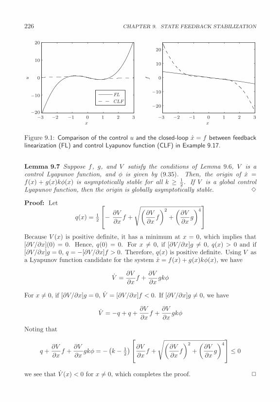
226 CHAPTER 9. STATE FEEDBACK STABILIZATION
−3 −2 −1 0 1 2 3−20
−10
0
10
20
x
u
FL
CLF
−3 −2 −1 0 1 2 3
−20
−10
0
10
20
x
f
Figure 9.1: Comparison of the control u and the closed-loop x = f between feedbacklinearization (FL) and control Lyapunov function (CLF) in Example 9.17.
Lemma 9.7 Suppose f , g, and V satisfy the conditions of Lemma 9.6, V is acontrol Lyapunov function, and φ is given by (9.35). Then, the origin of x =f(x) + g(x)kφ(x) is asymptotically stable for all k ≥ 1
2 . If V is a global controlLyapunov function, then the origin is globally asymptotically stable. �
Proof: Let
q(x) = 12
⎡⎣− ∂V
∂xf +
√(∂V
∂xf
)2
+(
∂V
∂xg
)4⎤⎦
Because V (x) is positive definite, it has a minimum at x = 0, which implies that[∂V/∂x](0) = 0. Hence, q(0) = 0. For x �= 0, if [∂V/∂x]g �= 0, q(x) > 0 and if[∂V/∂x]g = 0, q = −[∂V/∂x]f > 0. Therefore, q(x) is positive definite. Using V asa Lyapunov function candidate for the system x = f(x) + g(x)kφ(x), we have
V =∂V
∂xf +
∂V
∂xgkφ
For x �= 0, if [∂V/∂x]g = 0, V = [∂V/∂x]f < 0. If [∂V/∂x]g �= 0, we have
V = −q + q +∂V
∂xf +
∂V
∂xgkφ
Noting that
q +∂V
∂xf +
∂V
∂xgkφ = − (k − 1
2
)⎡⎣∂V
∂xf +
√(∂V
∂xf
)2
+(
∂V
∂xg
)4⎤⎦ ≤ 0
we see that V (x) < 0 for x �= 0, which completes the proof. �

9.8. EXERCISES 227
Example 9.18 In Example 9.17 we compared the feedback-linearization controlu = χ(x) = −x + x3 − αx with the control-Lyapunov-function formula u = φ(x) =−x+x3−x
√(1 − x2)2 + 1 for the system x = x−x3+u. According to Lemma 9.7 the
origin of the closed-loop system x = x−x3 +kφ(x) is globally asymptotically stablefor all k ≥ 1
2 . Let us study the gain margin of the system x = x − x3 + kχ(x). Asfar as local stabilization is concerned, the system has a gain margin (1/(1 + α),∞)because linearization as the origin yields x = −[k(1 + α) − 1]x. But, the originwill not be globally asymptotically stable for any k > 1 because for k > 1 thesystem has equilibrium points at 0 and ±√1 + kα/(k − 1). The region of attraction{−√1 + kα/(k − 1) < x <
√1 + kα/(k − 1))} shrinks toward {−√
1 + α < x <√1 + α} as k → ∞. �
9.8 Exercises
9.1 For each of the following systems, design a globally stabilizing state feedbackcontroller.
(1) x1 = x21 + x2, x2 = u
(2) x1 = x2, x2 = −x31 + sat(u)
(3) x1 = x1x2, x2 = u
(4) x1 = −x1 + tanh(x2), x2 = x2 + x3, x3 = u
(5) x1 = −x1 + x1x3, x2 = x3, x3 = x21 + u
(6) x1 = x31 + x2, x2 = x1x3 + u, x3 = x1x2 − x3
9.2 For each of the following systems, design a linear globally stabilizing statefeedback controller.
(1) x1 = x2, x2 = x1 + x2 − x31 + u
(2) x1 = sin x1 + x2, x2 = u
(3) x1 = −x31 + x2
2, x2 = u
(4) x1 = x2, x2 = −x2|x2| + u
(5) x1 = x2, x2 = sinx1 + u
9.3 For each of the following systems, it is required to design a state feedbackcontroller to globally stabilize the origin.
(a) Design the controller using feedback linearization.
(b) Design the controller using backstepping.

228 CHAPTER 9. STATE FEEDBACK STABILIZATION
(c) Compare the performance of the two controllers using simulation.
(1) x1 = x1 + x2/(1 + x21), x2 = −x2 + u
(2) x1 = sin x1 + x2, x2 = u
(3) x1 = x2 + 1 + (1 − x1)3, x2 = −x1 + u
9.4 Consider the inverted pendulum on a cart (A.41)–(A.44), where it is requiredto stabilize the pendulum at θ = 0 and the cart at y = 0.
(a) Show that the task cannot be achieved by open-loop control.
(b) Using linearization, design a stabilizing state feedback controller.
(c) Using simulation with the (A.45) data, find
(i) the range of x1(0), when x(0) = col(x1(0), 0, 0, 0), for which the pendulumis stabilized;
(ii) the effect of ±30% perturbation in m and J .
9.5 Consider the inverted pendulum (A.47), where it is required to stabilize thependulum at θ = 0 using state feedback.
(a) Design a stabilizing controller using linearization.
(b) Design a stabilizing controller using feedback linearization and determine itsdomain of validity.
(c) For each of the two controllers, use simulation with a = 1 to find the range ofx1(0), when x2(0) = 0, for which the pendulum is stabilized and |x1(t)| ≤ π/2for all t.
(d) Compare the performance of the two controllers.
9.6 Consider the controlled van der Pol equation (A.13). Design a globally stabi-lizing state feedback controller using
(a) feedback linearization
(b) backstepping
(c) feedback passivation and passivity based control
(d) control Lyapunov function, starting from the Lyapunov function of part (b).
9.7 Consider the biochemical reactor (A.19) with known ν(x2) given by (A.20).
(a) Using partial feedback linearization, design a state feedback controller suchthat x2 = −λ(x2 − 1) with λ > 0. Determine the region of validity of thecontroller.
9.8. EXERCISES 229
(b) Show that the controller of part (a) stabilizes the equilibrium point (x1 =1, x2 = 1) and estimate the region of attraction.
9.8 Consider the magnetic levitation system (A.30)–(A.32) with b = 0, c = 1,α = 1.5, and β = 2. It is required to stabilize the ball at x1 = 1.
(a) Find the steady-state input uss that maintains equilibrium at x1 = 1, and showthat the equilibrium point is unstable under the open-loop control u = uss.
In the rest of this exercise we design three different state feedback controllers. Usingsimulation, choose the controller parameters in each case to have a settling time lessthan 20 time units, following a small perturbation from the equilibrium point, andfind the range of x1(0), when the other states start from their equilibrium values,for which the ball will be stabilized at x1 = 1.
(b) Design a controller using linearization.
(c) Transform the state equation into the controller form and determine the domainof validity of the transformation.
(d) Design a controller using feedback linearization.
(e) Starting from the controller form, design a controller using backstepping.
(f) Compare the performance of the three controllers when x(0) = col(2, 0, 1.5).
9.9 Consider the electrostatic microactuator (A.33). It is required to stabilize theplate at x1 = r < 1.
(a) By studying the equilibrium points for a constant input u = u < 1, determinethe restrictions on r and the region of attraction if the system is to be operatedwithout feedback control.
In the rest of this exercise let r = 0.5, ζ = 0.1, and T = 0.2. We design four differ-ent state feedback controllers. Using simulation, choose the controller parametersin each case so that |u(t)| ≤ 2 when x(0) = col(0.1, 0.
√0.3). For this choice of
parameters, let x(0) = col(α, 0,√
3α) and find the range of α for which x(0) belongsto the region of attraction if the control was not constrained.
(b) Design a controller using linearization.
(c) Transform the state equation into the controller form and determine the domainof validity of the transformation.
(d) Design a controller using feedback linearization.
(e) Starting from the controller form, design a controller using backstepping.

230 CHAPTER 9. STATE FEEDBACK STABILIZATION
(f) Using partial feedback linearization to convert the x3-equation into x3 = v,and then shifting the desired equilibrium point to the origin, show that thesystem can be represented in the form (9.23)–(9.25) and the conditions ofTheorem 9.2 are satisfied.
(g) Design a controller using passivity-based control.
(h) Compare the performance of the four controllers.
9.10 Consider the boost converter (A.16).
(a) Show that, with u = 0, the open-loop system is linear and has an asymptoticallystable origin.
(b) Using passivity-based control, design a state feedback controller such that theorigin is globally asymptotically stable, 0 < μ = u + 1 − 1/k < 1, and theclosed-loop system has more damping than the open-loop one.
(c) Simulate the open-loop and closed-loop systems with α = 0.1, k = 2, x1(0) =−0.7/4, and x2(0) = − 1
2 .
9.11 Consider the DC motor (A.25) with δ = 0 and f�(x3) = bx3 where b ≥ 0. Itis desired to design a state feedback controller to stabilize the speed at ω∗.
(a) Transform equation (A.25) into the normal form, as described in Example 8.6.
(b) Using partial feedback linearization bring the external part of the normal forminto ξ1 = ξ2, ξ2 = v and determine its domain of validity.
(c) Find the equilibrium point at which ω = ω∗.
(d) Design a state feedback controller for v to stabilize the equilibrium point andfind under what conditions is the controller valid.
9.12 Consider the two-link manipulator defined by (A.36) and (A.37) with the(A.38) data. It is desired to regulate the manipulator to qr = (π/2, π/2) under thecontrol constraints |u1| ≤ 6000 and |u2| ≤ 5000.
(a) Apply the passivity-based controller of Example 9.15. Use simulation to choosethe controller parameters to meet the control constraints.
(b) Design a feedback-linearization controller based on Example 8.7. Use simula-tion to choose the controller parameters to meet the control constraints.
(c) Compare the performance of the two controllers under the nominal parametersof (A.38) and the perturbed parameters of (A.39).
9.13 Consider the TORA system of (A.49)–(A.52). Show that the origin can beglobally stabilized by u = −φ1(x1) − φ2(x2) where φ1 and φ2 are locally Lips-chitz functions that satisfy φi(0) = 0 and yφi(y) > 0 for all y �= 0. Hint: SeeExercise 5.10.
Chapter 10
Robust State Feedback Stabilization
The stabilization techniques of Chapter 9, except possibly for passivity-based con-trol, require a good model of the system. Perturbation analysis of the closed-loopsystem determines the level of model uncertainty that can be tolerated while main-taining asymptotic stability. However, the level of model uncertainty cannot beprescribed. The robust stabilization techniques of this chapter can ensure stabiliza-tion under “large” matched uncertainties provided upper bounds on the uncertainterms are known. The uncertainty is matched when the uncertain terms enter thestate equation at the same point as the control input, which allows the control todominate their effect.
Three robust stabilization techniques are presented in this chapter. In the slidingmode control of Section 10.1, a sliding manifold, independent of model uncertainty,is designed such that trajectories on the manifold converge to the equilibrium point.Then, the control is designed to force all trajectories to reach the manifold in finitetime and stay on it for all future time. The control uses only upper bounds onthe uncertain terms. In the Lyapunov redesign of Section 10.2, a stabilizing con-trol is designed first for a nominal model with no uncertainty. Then, a Lyapunovfunction of the nominal closed-loop system is used to design an additional controlcomponent that makes the design robust to matched uncertainties. Both slidingmode control and Lyapunov redesign produce discontinuous feedback controllers,which poses theoretical as well as practical challenges. Theoretically, the right-handside function of the closed-loop system will not be locally Lipschitz, which is theunderlying assumption for the theory presented in this book. Practically, the im-plementation of such discontinuous controllers is characterized by the phenomenonof chattering. Therefore, in Section 10.1 and 10.2 we develop continuous approxi-mations of the discontinuous controllers. In Section 10.3, we show how to achieverobust stabilization by high-gain feedback.
When the uncertain terms do not vanish at the equilibrium point, locally Lips-chitz feedback controllers cannot stabilize the equilibrium point but can bring thetrajectories arbitrarily close to it. This is known as practical stabilization, which is
231
232 CHAPTER 10. ROBUST STATE FEEDBACK STABILIZATION
defined next for the system
x = f(x, u) + δ(t, x, u)
where f(0, 0) = 0 and δ(t, 0, 0) �= 0. For a locally Lipschitz feedback control u =φ(x), with φ(0) = 0, the origin x = 0 is not an equilibrium point of the closed-loopsystem x = f(x, φ(x)) + δ(t, x, φ(x)).
Definition 10.1 The system x = f(x, u) + δ(t, x, u) is said to be practically stabi-lizable by the feedback control u = φ(x) if for every b > 0, the control can be designedsuch that the solutions are ultimately bounded by b; that is
‖x(t)‖ ≤ b, ∀ t ≥ T
for some T > 0.
Typically, the control u = φ(x) depends on a design parameter that can be chosen toachieve the ultimate bound b. In Section 9.1 we defined four notions of stabilizationdepending on the region of initial states. With practical stabilization, we can use thesame notions and talk of local, regional, global or semiglobal practical stabilization.For example, the system is semiglobally practically stabilizable by the feedbackcontrol u = φ(x) if given any compact set G and any b > 0, φ(x) can be designedto ensure that for all initial states in G, the solutions are ultimately bounded by b.
10.1 Sliding Mode Control
We start with a motivating example, then present the theory for n-dimensionalmulti-input systems.
Example 10.1 Consider the two-dimensional, single-input system
x1 = x2, x2 = h(x) + g(x)u
where h and g are unknown locally Lipschitz functions and g(x) ≥ g0 > 0 for all x.We want to design a state feedback controller to stabilize the origin. Suppose wecan design a controller that constrains the trajectory to the manifold (or surface)s = ax1 + x2 = 0, where the motion is governed by x1 = −ax1. Choosing a > 0guarantees that x(t) tends to zero as t tends to infinity and the rate of convergencecan be controlled by choice of a. The motion on the manifold s = 0 is independentof h and g. How can we bring the trajectory to this manifold and maintain it there?The variable s satisfies the equation
s = ax1 + x2 = ax2 + h(x) + g(x)u
Suppose h and g satisfy the inequality∣∣∣∣ax2 + h(x)g(x)
∣∣∣∣ ≤ �(x), ∀ x ∈ R2
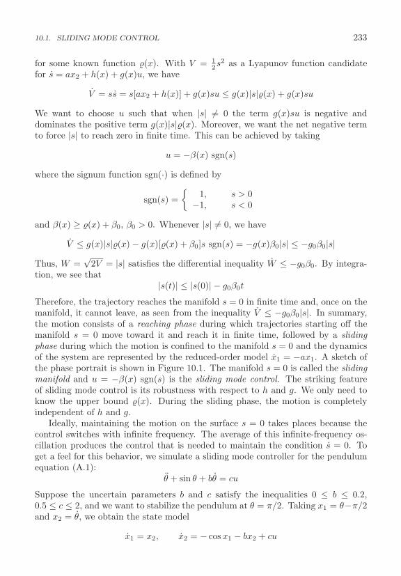
10.1. SLIDING MODE CONTROL 233
for some known function �(x). With V = 12s2 as a Lyapunov function candidate
for s = ax2 + h(x) + g(x)u, we have
V = ss = s[ax2 + h(x)] + g(x)su ≤ g(x)|s|�(x) + g(x)su
We want to choose u such that when |s| �= 0 the term g(x)su is negative anddominates the positive term g(x)|s|�(x). Moreover, we want the net negative termto force |s| to reach zero in finite time. This can be achieved by taking
u = −β(x) sgn(s)
where the signum function sgn(·) is defined by
sgn(s) ={
1, s > 0−1, s < 0
and β(x) ≥ �(x) + β0, β0 > 0. Whenever |s| �= 0, we have
V ≤ g(x)|s|�(x) − g(x)[�(x) + β0]s sgn(s) = −g(x)β0|s| ≤ −g0β0|s|Thus, W =
√2V = |s| satisfies the differential inequality W ≤ −g0β0. By integra-
tion, we see that|s(t)| ≤ |s(0)| − g0β0t
Therefore, the trajectory reaches the manifold s = 0 in finite time and, once on themanifold, it cannot leave, as seen from the inequality V ≤ −g0β0|s|. In summary,the motion consists of a reaching phase during which trajectories starting off themanifold s = 0 move toward it and reach it in finite time, followed by a slidingphase during which the motion is confined to the manifold s = 0 and the dynamicsof the system are represented by the reduced-order model x1 = −ax1. A sketch ofthe phase portrait is shown in Figure 10.1. The manifold s = 0 is called the slidingmanifold and u = −β(x) sgn(s) is the sliding mode control. The striking featureof sliding mode control is its robustness with respect to h and g. We only need toknow the upper bound �(x). During the sliding phase, the motion is completelyindependent of h and g.
Ideally, maintaining the motion on the surface s = 0 takes places because thecontrol switches with infinite frequency. The average of this infinite-frequency os-cillation produces the control that is needed to maintain the condition s = 0. Toget a feel for this behavior, we simulate a sliding mode controller for the pendulumequation (A.1):
θ + sin θ + bθ = cu
Suppose the uncertain parameters b and c satisfy the inequalities 0 ≤ b ≤ 0.2,0.5 ≤ c ≤ 2, and we want to stabilize the pendulum at θ = π/2. Taking x1 = θ−π/2and x2 = θ, we obtain the state model
x1 = x2, x2 = − cos x1 − bx2 + cu
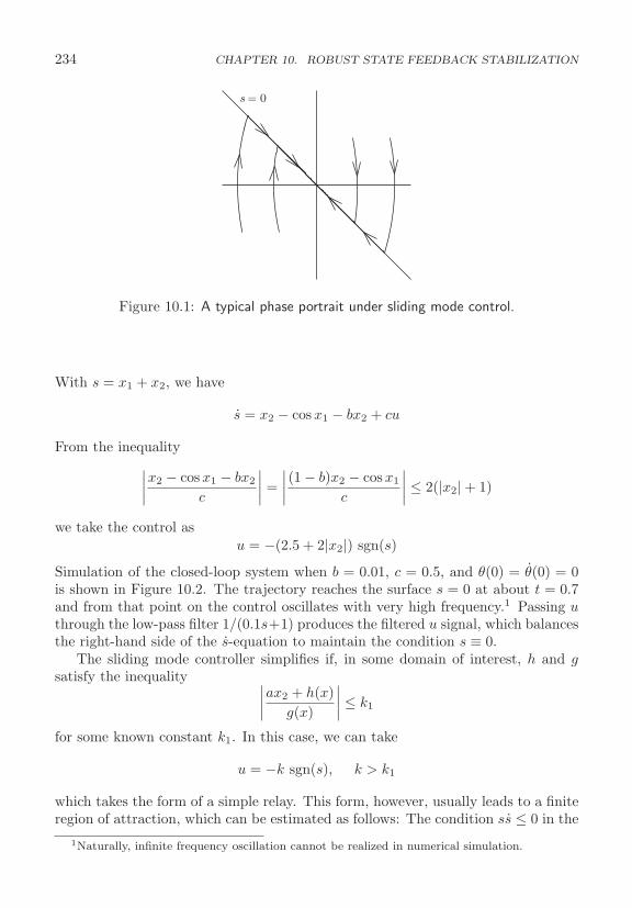
234 CHAPTER 10. ROBUST STATE FEEDBACK STABILIZATION
s= 0
Figure 10.1: A typical phase portrait under sliding mode control.
With s = x1 + x2, we have
s = x2 − cos x1 − bx2 + cu
From the inequality∣∣∣∣x2 − cos x1 − bx2
c
∣∣∣∣ =∣∣∣∣ (1 − b)x2 − cos x1
c
∣∣∣∣ ≤ 2(|x2| + 1)
we take the control asu = −(2.5 + 2|x2|) sgn(s)
Simulation of the closed-loop system when b = 0.01, c = 0.5, and θ(0) = θ(0) = 0is shown in Figure 10.2. The trajectory reaches the surface s = 0 at about t = 0.7and from that point on the control oscillates with very high frequency.1 Passing uthrough the low-pass filter 1/(0.1s+1) produces the filtered u signal, which balancesthe right-hand side of the s-equation to maintain the condition s ≡ 0.
The sliding mode controller simplifies if, in some domain of interest, h and gsatisfy the inequality ∣∣∣∣ax2 + h(x)
g(x)
∣∣∣∣ ≤ k1
for some known constant k1. In this case, we can take
u = −k sgn(s), k > k1
which takes the form of a simple relay. This form, however, usually leads to a finiteregion of attraction, which can be estimated as follows: The condition ss ≤ 0 in the
1Naturally, infinite frequency oscillation cannot be realized in numerical simulation.
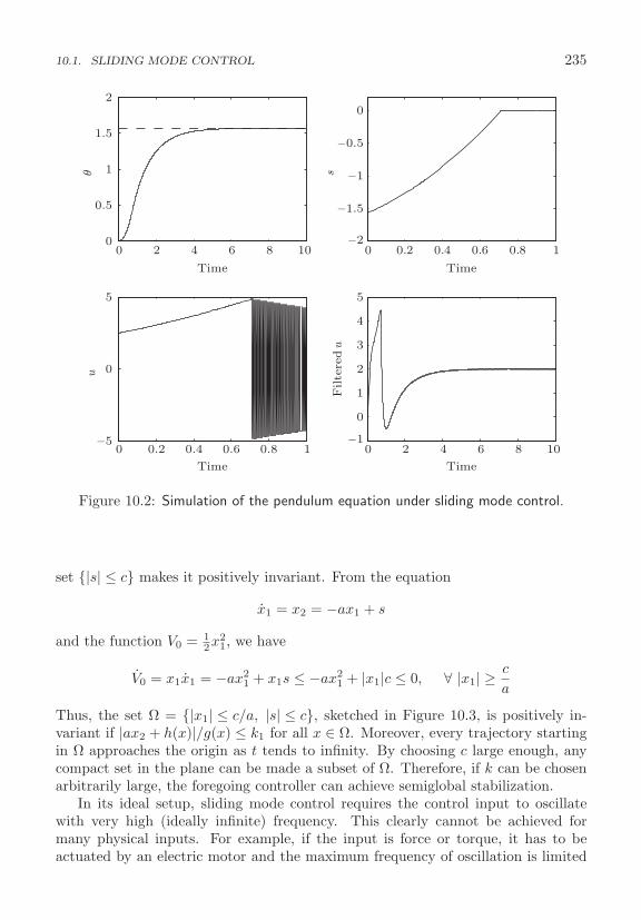
10.1. SLIDING MODE CONTROL 235
0 2 4 6 8 10
Time
θ
0 0.2 0.4 0.6 0.8 1−2
−1.5
−1
−0.5
0
Time
s
0 0.2 0.4 0.6 0.8 1
0
0.5
1
1.5
2
−5
0
5
Time
u
0 2 4 6 8 10−1
0
1
2
3
4
5
Time
Filte
red u
Figure 10.2: Simulation of the pendulum equation under sliding mode control.
set {|s| ≤ c} makes it positively invariant. From the equation
x1 = x2 = −ax1 + s
and the function V0 = 12x2
1, we have
V0 = x1x1 = −ax21 + x1s ≤ −ax2
1 + |x1|c ≤ 0, ∀ |x1| ≥ c
a
Thus, the set Ω = {|x1| ≤ c/a, |s| ≤ c}, sketched in Figure 10.3, is positively in-variant if |ax2 + h(x)|/g(x) ≤ k1 for all x ∈ Ω. Moreover, every trajectory startingin Ω approaches the origin as t tends to infinity. By choosing c large enough, anycompact set in the plane can be made a subset of Ω. Therefore, if k can be chosenarbitrarily large, the foregoing controller can achieve semiglobal stabilization.
In its ideal setup, sliding mode control requires the control input to oscillatewith very high (ideally infinite) frequency. This clearly cannot be achieved formany physical inputs. For example, if the input is force or torque, it has to beactuated by an electric motor and the maximum frequency of oscillation is limited
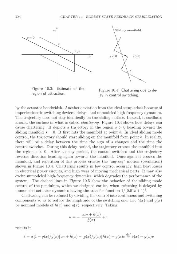
236 CHAPTER 10. ROBUST STATE FEEDBACK STABILIZATION
s= 0
c/a
c
x2
x1
Figure 10.3: Estimate of theregion of attraction.
Sliding manifold
b
s > 0s < 0
Figure 10.4: Chattering due to de-lay in control switching.
by the actuator bandwidth. Another deviation from the ideal setup arises because ofimperfections in switching devices, delays, and unmodeled high-frequency dynamics.The trajectory does not stay identically on the sliding surface. Instead, it oscillatesaround the surface in what is called chattering. Figure 10.4 shows how delays cancause chattering. It depicts a trajectory in the region s > 0 heading toward thesliding manifold s = 0. It first hits the manifold at point b. In ideal sliding modecontrol, the trajectory should start sliding on the manifold from point b. In reality,there will be a delay between the time the sign of s changes and the time thecontrol switches. During this delay period, the trajectory crosses the manifold intothe region s < 0. After a delay period, the control switches and the trajectoryreverses direction heading again towards the manifold. Once again it crosses themanifold, and repetition of this process creates the “zig-zag” motion (oscillation)shown in Figure 10.4. Chattering results in low control accuracy, high heat lossesin electrical power circuits, and high wear of moving mechanical parts. It may alsoexcite unmodeled high-frequency dynamics, which degrades the performance of thesystem. The dashed lines in Figure 10.5 show the behavior of the sliding modecontrol of the pendulum, which we designed earlier, when switching is delayed byunmodeled actuator dynamics having the transfer function 1/(0.01s + 1)2.
Chattering can be reduced by dividing the control into continuous and switchingcomponents so as to reduce the amplitude of the switching one. Let h(x) and g(x)be nominal models of h(x) and g(x), respectively. Taking
u = − ax2 + h(x)g(x)
+ v
results in
s = a [1 − g(x)/g(x)]x2 + h(x) − [g(x)/g(x)] h(x) + g(x)v def= δ(x) + g(x)v
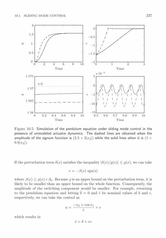
10.1. SLIDING MODE CONTROL 237
0 2 4 6 8 100
0.5
1
1.5
2θ
θ
0 1 2 3−2
−1.5
−1
−0.5
0
s
9 9.2 9.4 9.6 9.8 101.56
1.565
1.57
1.575
9.5 9.6 9.7 9.8 9.9 10−15
−10
−5
0
5
s
Time
TimeTime
Time
x 10−3
π/2
Figure 10.5: Simulation of the pendulum equation under sliding mode control in thepresence of unmodeled actuator dynamics. The dashed lines are obtained when theamplitude of the signum function is (2.5 + 2|x2|) while the solid lines when it is (1 +0.8|x2|).
If the perturbation term δ(x) satisfies the inequality |δ(x)/g(x)| ≤ �(x), we can take
v = −β(x) sgn(s)
where β(x) ≥ �(x)+β0. Because � is an upper bound on the perturbation term, it islikely to be smaller than an upper bound on the whole function. Consequently, theamplitude of the switching component would be smaller. For example, returningto the pendulum equation and letting b = 0 and c be nominal values of b and c,respectively, we can take the control as
u =−x2 + cos x1
c+ v
which results ins = δ + cv
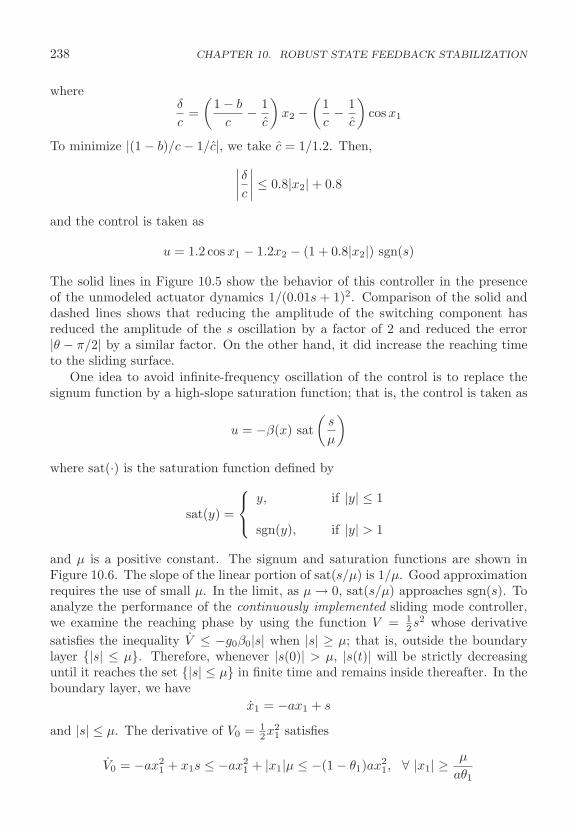
238 CHAPTER 10. ROBUST STATE FEEDBACK STABILIZATION
whereδ
c=(
1 − b
c− 1
c
)x2 −
(1c− 1
c
)cos x1
To minimize |(1 − b)/c − 1/c|, we take c = 1/1.2. Then,∣∣∣∣δc∣∣∣∣ ≤ 0.8|x2| + 0.8
and the control is taken as
u = 1.2 cos x1 − 1.2x2 − (1 + 0.8|x2|) sgn(s)
The solid lines in Figure 10.5 show the behavior of this controller in the presenceof the unmodeled actuator dynamics 1/(0.01s + 1)2. Comparison of the solid anddashed lines shows that reducing the amplitude of the switching component hasreduced the amplitude of the s oscillation by a factor of 2 and reduced the error|θ − π/2| by a similar factor. On the other hand, it did increase the reaching timeto the sliding surface.
One idea to avoid infinite-frequency oscillation of the control is to replace thesignum function by a high-slope saturation function; that is, the control is taken as
u = −β(x) sat(
s
μ
)
where sat(·) is the saturation function defined by
sat(y) =
⎧⎨⎩
y, if |y| ≤ 1
sgn(y), if |y| > 1
and μ is a positive constant. The signum and saturation functions are shown inFigure 10.6. The slope of the linear portion of sat(s/μ) is 1/μ. Good approximationrequires the use of small μ. In the limit, as μ → 0, sat(s/μ) approaches sgn(s). Toanalyze the performance of the continuously implemented sliding mode controller,we examine the reaching phase by using the function V = 1
2s2 whose derivativesatisfies the inequality V ≤ −g0β0|s| when |s| ≥ μ; that is, outside the boundarylayer {|s| ≤ μ}. Therefore, whenever |s(0)| > μ, |s(t)| will be strictly decreasinguntil it reaches the set {|s| ≤ μ} in finite time and remains inside thereafter. In theboundary layer, we have
x1 = −ax1 + s
and |s| ≤ μ. The derivative of V0 = 12x2
1 satisfies
V0 = −ax21 + x1s ≤ −ax2
1 + |x1|μ ≤ −(1 − θ1)ax21, ∀ |x1| ≥ μ
aθ1

10.1. SLIDING MODE CONTROL 239
sgn (y) sat (y/μ)
y yμ
−1−1
1 1
Figure 10.6: The signum nonlinearity and its saturation function approximation.
where 0 < θ1 < 1. Thus, the trajectory reaches the set Ωμ = {|x1| ≤ μ/(aθ1), |s| ≤μ} in finite time. In general, the controller does not stabilize the origin, but achievespractical stabilization because the ultimate bound can be reduced by decreasing μ.For better accuracy, we need to choose μ as small as possible, but a too smallvalue of μ will induce chattering in the presence of time delays or unmodeled fastdynamics. Figure 10.7 shows the performance of the pendulum equation under thecontinuously implemented sliding mode controller
u = −(2.5 + 2|x2|) sat(s/μ)
for two different values of μ, with and without the unmodeled actuator 1/(0.01s +1)2. In the absence of actuator dynamics, reducing μ does indeed bring s close tozero and reduces the error |θ−π/2|. However, in the presence of actuator dynamics,the smaller value of μ induces chattering of s.
One special case where we can stabilize the origin without pushing μ too smallarises when h(0) = 0. In this case, the system, represented inside the boundarylayer by
x1 = x2, x2 = h(x) − [g(x)β(x)/μ] (ax1 + x2)
has an equilibrium point at the origin. We need to choose μ small enough to stabilizethe origin and make Ωμ a subset of its region of attraction. To illustrate this point,consider the stabilization of the pendulum at θ = π. With x1 = θ − π, x2 = θ, ands = x1 + x2, we obtain
s = x2 + sinx1 − bx2 + cu
Once again, assuming 0 ≤ b ≤ 0.2 and 0.5 ≤ c ≤ 2, it can be shown that∣∣∣∣ (1 − b)x2 + sin x1
c
∣∣∣∣ ≤ 2(|x1| + |x2|)

240 CHAPTER 10. ROBUST STATE FEEDBACK STABILIZATION
0 2 4 6 8 100
0.5
1
1.5
2
Time
9.5 9.6 9.7 9.8 9.9 10−0.1
−0.05
0
0.05
0.1
Time
0 2 4 6 8 100
0.5
1
1.5
2
Time
9.5 9.6 9.7 9.8 9.9 10−0.1
−0.05
0
0.05
0.1
Time
θθ
ss
(a) (b)
(c) (d)
μ= 0.1
μ= 0.001
Figure 10.7: Simulation of the pendulum equation under continuously-implementedsliding mode control without ((a) and (b)) and with ((c) and (d)) unmodeled actuatordynamics.
Therefore, the control is taken as
u = −2(|x1| + |x2| + 1) sat(s/μ)
Inside the boundary layer {|s| ≤ μ}, the system is given by
x1 = −x1 + s, s = (1 − b)x2 + sin x1 − 2c(|x1| + |x2| + 1)s/μ
and has an equilibrium point at the origin. The derivative of the Lyapunov functioncandidate V1 = 1
2x21 + 1
2s2 satisfies
V1 = −x21 + x1s + (1 − b)(s − x1)s + s sin x1 − 2c(|x1| + |x2| + 1)s2/μ
≤ −x21 + 3|x1| |s| − (1/μ − 1)s2 = −
[|x1||s|]T [ 1 −3/2
−3/2 (1/μ − 1)
] [|x1||s|]
10.1. SLIDING MODE CONTROL 241
Choosing μ < 4/13 = 0.308 makes V1 negative definite; hence, the origin is asymp-totically stable. �
Consider the system
x = f(x) + B(x)[G(x)u + δ(t, x, u)] (10.1)
where x ∈ Rn is the state, u ∈ Rm is the control input, f , B, and G are suf-ficiently smooth functions in a domain D ⊂ Rn that contains the origin, andG(x) is a positive definite symmetric matrix whose minimum eigenvalue satisfiesλmin(G(x)) ≥ λ0 > 0, for all x ∈ D. The function δ is piecewise continuous in tand sufficiently smooth in (x, u) for (t, x, u) ∈ [0,∞)×D ×Rm. We assume that fand B are known, while G and δ could be uncertain. Suppose f(0) = 0 so that, inthe absence of δ, the origin is an open-loop equilibrium point. Our goal is to designa state feedback controller to stabilize the origin for all uncertainties in G and δ.
Let T : D → Rn be a diffeomorphism such that
∂T
∂xB(x) =
[0I
](10.2)
where I is the m × m identity matrix.2 The change of variables[ηξ
]= T (x), η ∈ Rn−m, ξ ∈ Rm (10.3)
transforms the system into the form
η = fa(η, ξ), ξ = fb(η, ξ) + G(x)u + δ(t, x, u) (10.4)
The form (10.4) is usually referred to as the regular form. To design the slidingmode controller, we start by designing the sliding manifold s = ξ − φ(η) = 0 suchthat, when motion is restricted to the manifold, the reduced-order model
η = fa(η, φ(η)) (10.5)
has an asymptotically stable equilibrium point at the origin. The design of φ(η)amounts to solving a stabilization problem for the system η = fa(η, ξ) with ξ viewedas the control input. We assume that we can find a stabilizing, sufficiently smoothfunction φ(η) with φ(0) = 0. Next, we design u to bring s to zero in finite time andmaintain it there for future time. Toward that end, let us write the s-equation:
s = fb(η, ξ) − ∂φ
∂ηfa(η, ξ) + G(x)u + δ(t, x, u) (10.6)
2If B(x) has full rank and the span of its columns is involutive, then Frobenius theorem [66]ensures local existence of T (x) in the neighborhood of each point in D. If B is independent of xand has full rank, then T (x) exists globally and takes the form T (x) = Lx where LB = col(0, I).
242 CHAPTER 10. ROBUST STATE FEEDBACK STABILIZATION
As we saw in Example 10.1, we can design u as a pure switching component or it maycontain an additional continuous component. If G(x) is a nominal model of G(x),the continuous component of u could be −G−1[fb − (∂φ/∂η)fa]. In the absence ofuncertainty; that is, when δ = 0 and G is known, taking u = −G−1[fb − (∂φ/∂η)fa]results in s = 0, which ensures that s = 0 is an invariant manifold. We take thecontrol u as
u = ψ(η, ξ) + v (10.7)
where typical choices of ψ are ψ = 0 and ψ = −G−1[fb − (∂φ/∂η)fa]. Other choicesof ψ would arise if, for example, we decide to cancel part of the known term onthe right-hand side of (10.6) rather than the whole term. Substituting (10.7) into(10.6) yields
s = G(x)v + Δ(t, x, v) (10.8)
where
Δ(t, x, v) = fb(η, ξ) − ∂φ
∂ηfa(η, ξ) + G(x)ψ(η, ξ) + δ(t, x, ψ(η, ξ) + v)
Assume we know a locally Lipschitz function �(x) ≥ 0 and a constant κ0, 0 ≤ κ0 < 1,such that∥∥∥∥ Δ(t, x, v)
λmin(G(x))
∥∥∥∥ ≤ �(x) + κ0‖v‖, ∀ (t, x, v) ∈ [0,∞) × D × Rm (10.9)
Utilizing V = 12sT s as a Lyapunov function candidate for (10.8), we obtain
V = sT s = sT G(x)v + sT Δ(t, x, v)
Takingv = −β(x)
s
‖s‖ (10.10)
where β is a locally Lipschitz function that satisfies
β(x) ≥ �(x)1 − κ0
+ β0, ∀ x ∈ D (10.11)
for some β0 > 0, yields
V = −β(x)sT G(x)s/‖s‖ + sT Δ(t, x, v)≤ λmin(G(x))[−β(x) + �(x) + κ0β(x)] ‖s‖= λmin(G(x))[−(1 − κ0)β(x) + �(x)] ‖s‖ ≤ −λmin(G(x))β0(1 − κ0)‖s‖≤ −λ0β0(1 − κ0)‖s‖
The inequality V ≤ −λ0β0(1 − κ0)‖s‖ = −λ0β0(1 − κ0)√
2V ensures that all tra-jectories starting off the manifold s = 0 reach it in finite time and those on themanifold cannot leave it.
The procedure for designing a sliding mode stabilizing controller can be sum-marized by the following steps:
10.1. SLIDING MODE CONTROL 243
• Design the sliding manifold ξ = φ(η) to stabilize the reduced-order system(10.5).
• Take the control u = ψ(η, ξ) + v, where typical choices of ψ are ψ = 0 andψ = −G−1[fb − (∂φ/∂η)fa].
• Estimate �(x) and κ0 in (10.9), where Δ depends on the choice of ψ in theprevious step.
• Choose β(x) that satisfies (10.11) and take the switching (discontinuous) con-trol v as given by (10.10).
This procedure exhibits model-order reduction because the main design task is per-formed on the reduced-order system (10.5). The key feature of sliding mode controlis its robustness to matched uncertainties. During the reaching phase, the taskof forcing the trajectories toward the sliding manifold and maintaining them thereis achieved by the switching control (10.10), provided β(x) satisfies the inequality(10.11). From (10.9), we see that �(x) is a measure of the size of the uncertainty.Since we do not require �(x) to be small, the switching controller can handle fairlylarge uncertainties, limited only by practical constraints on the amplitude of thecontrol signals. During the sliding phase, the motion of the system, as determinedby (10.5), is independent of the matched uncertain terms G and δ.
The sliding mode controller contains the discontinuous function s/‖s‖, whichreduces to the signum function sgn(s) when s is scalar. The discontinuity of thecontroller raises theoretical as well as practical issues. Theoretical issues like ex-istence and uniqueness of solutions and validity of Lyapunov analysis will have tobe examined in a framework that does not require the state equation to have lo-cally Lipschitz right-hand-side functions.3 There are also practical issues like thetrajectory chattering around the sliding surface due to imperfections of switchingdevices, delays, and unmodeled high-frequency dynamics, as illustrated in Exam-ple 10.1, and the inability of the control to oscillate with very high frequency dueto limited actuator bandwidth. To avoid these issues we use a continuous approxi-mation of s/‖s‖.4 Define the vector saturation function Sat(y) by
Sat(y) =
⎧⎨⎩
y, if ‖y‖ ≤ 1
y/‖y‖, if ‖y‖ > 1
3To read about differential equations with discontinuous right-hand side, consult [38, 102, 122,151].
4See [106, 124, 142, 153] for a deeper study of sliding mode control and different approachesto deal with these practical issues. While we do not pursue rigorous analysis of the discontinuoussliding mode controller, the reader is encouraged to use simulation to examine the performance ofboth the discontinuous controller and its continuous implementation.
244 CHAPTER 10. ROBUST STATE FEEDBACK STABILIZATION
It can be verified that Sat(y) is locally Lipschitz. We approximate s/‖s‖ by Sat(s/μ)with small positive constant μ;5 that is,
v = −β(x) Sat(
s
μ
)(10.12)
where β(x) satisfies (10.11). In the region ‖s‖ ≥ μ, Sat(s/μ) = s/‖s‖. Therefore,
sT s ≤ −λ0β0(1 − κ0)‖s‖which shows that whenever ‖s(0)‖ > μ, ‖s(t)‖ will decrease until it reaches theset {‖s‖ ≤ μ} in finite time and remains inside thereafter. The set {‖s‖ ≤ μ} iscalled the boundary layer. To study the behavior of η, we assume that there is a(continuously differentiable) Lyapunov function V0(η) that satisfies the inequalities
α1(‖η‖) ≤ V0(η) ≤ α2(‖η‖) (10.13)
∂V0
∂ηfa(η, φ(η) + s) ≤ −α3(‖η‖), ∀ ‖η‖ ≥ α4(‖s‖) (10.14)
for all (η, ξ) ∈ T (D), where α1 to α4 are class K functions.6 Noting that
‖s‖ ≤ c ⇒ V0 ≤ −α3(‖η‖), for ‖η‖ ≥ α4(c)
we define a class K function α by α = α2 ◦ α4. Then,
V0(η) ≥ α(c) ⇔ V0(η) ≥ α2(α4(c)) ⇒ α2(‖η‖) ≥ α2(α4(c))⇒ ‖η‖ ≥ α4(c) ⇒ V0 ≤ −α3(‖η‖) ≤ −α3(α4(c))
which shows that the set {V (η) ≤ c0} with c0 ≥ α(c) is positively invariant becauseV is negative on the boundary V (η) = c0. (See Figure 10.8.) It follows that the set
Ω = {V0(η) ≤ c0} × {‖s‖ ≤ c}, with c0 ≥ α(c) (10.15)
is positively invariant whenever c > μ and Ω ⊂ T (D). Choose μ, c, and c0 such thatc > μ, c0 ≥ α(c), and Ω is compact and contained in T (D). The set Ω serves as ourestimate of the “region of attraction.” For all initial states in Ω, the trajectorieswill be bounded for all t ≥ 0. After some finite time, we have ‖s(t)‖ ≤ μ. It followsfrom the foregoing analysis that V0 ≤ −α3(α4(μ)) for all V0(η) ≥ α(μ). Hence, thetrajectories will reach the positively invariant set
Ωμ = {V0(η) ≤ α(μ)} × {‖s‖ ≤ μ} (10.16)
in finite time. The set Ωμ can be made arbitrarily small by choosing μ smallenough, which shows that the continuously implemented sliding mode controller
5Smooth approximations are discussed in Exercise 14.11 of [74].6By Theorem 4.7, inequality (10.14) implies regional input-to-state stability of the system
η = fa(η, φ(η) + s) when s is viewed as the input.
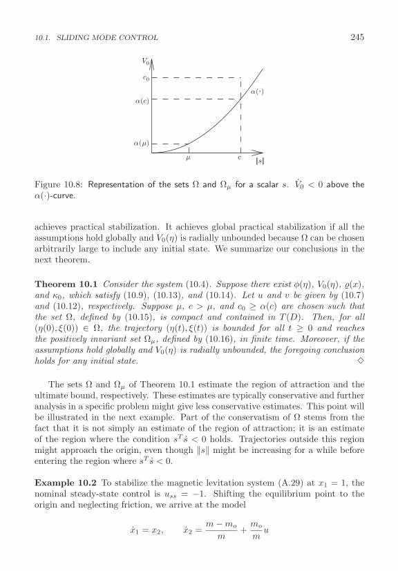
10.1. SLIDING MODE CONTROL 245
α (.)α (c)
α (μ)
IsIcμ
V0
c0
Figure 10.8: Representation of the sets Ω and Ωμ for a scalar s. V0 < 0 above theα(·)-curve.
achieves practical stabilization. It achieves global practical stabilization if all theassumptions hold globally and V0(η) is radially unbounded because Ω can be chosenarbitrarily large to include any initial state. We summarize our conclusions in thenext theorem.
Theorem 10.1 Consider the system (10.4). Suppose there exist φ(η), V0(η), �(x),and κ0, which satisfy (10.9), (10.13), and (10.14). Let u and v be given by (10.7)and (10.12), respectively. Suppose μ, c > μ, and c0 ≥ α(c) are chosen such thatthe set Ω, defined by (10.15), is compact and contained in T (D). Then, for all(η(0), ξ(0)) ∈ Ω, the trajectory (η(t), ξ(t)) is bounded for all t ≥ 0 and reachesthe positively invariant set Ωμ, defined by (10.16), in finite time. Moreover, if theassumptions hold globally and V0(η) is radially unbounded, the foregoing conclusionholds for any initial state. �
The sets Ω and Ωμ of Theorem 10.1 estimate the region of attraction and theultimate bound, respectively. These estimates are typically conservative and furtheranalysis in a specific problem might give less conservative estimates. This point willbe illustrated in the next example. Part of the conservatism of Ω stems from thefact that it is not simply an estimate of the region of attraction; it is an estimateof the region where the condition sT s < 0 holds. Trajectories outside this regionmight approach the origin, even though ‖s‖ might be increasing for a while beforeentering the region where sT s < 0.
Example 10.2 To stabilize the magnetic levitation system (A.29) at x1 = 1, thenominal steady-state control is uss = −1. Shifting the equilibrium point to theorigin and neglecting friction, we arrive at the model
x1 = x2, x2 =m − mo
m+
mo
mu
246 CHAPTER 10. ROBUST STATE FEEDBACK STABILIZATION
under the constraints x1 ≥ −1 and |u| ≤ 1. Suppose that |(m − mo)/mo| ≤ 13 .
Taking s = x1 + x2 yields x1 = −x1 + s. The derivative of V0 = 12x2
1 satisfies
V0 = −x21 + x1s ≤ −(1 − θ)x2
1, ∀ |x1| ≥ |s|/θ
where 0 < θ < 1. Thus, V0 satisfies (10.13) and (10.14) with α1(r) = α2(r) = 12r2,
α3(r) = (1 − θ)r2, and α4(r) = r/θ. Hence, α(r) = 12 (r/θ)2. With c0 = α(c), the
sets Ω and Ωμ of (10.15) and (10.16) are given by
Ω = {|x1| ≤ c/θ} × {|s| ≤ c}, Ωμ = {|x1| ≤ μ/θ} × {|s| ≤ μ}
To meet the constraint x1 ≥ −1, c is limited to c ≤ θ. From
s = x2 +m − mo
m+
mo
mu
we see that (10.9) takes the form∣∣∣∣x2 + (m − mo)/m
mo/m
∣∣∣∣ =∣∣∣∣ m
mox2 +
m − mo
mo
∣∣∣∣ ≤ 13 (4|x2| + 1)
We limit our analysis to the set Ω where |x2| ≤ |x1| + |s| ≤ c(1 + 1/θ). With1/θ = 1.1, the foregoing inequality takes the form∣∣∣∣x2 + (m − mo)/m
mo/m
∣∣∣∣ ≤ 8.4c + 13
To meet the constraint |u| ≤ 1, we take u = −sat(s/μ). Then, inequality (10.11)limits c to
8.4c + 13
< 1 ⇔ c < 0.238
With c = 0.23, Theorem 10.1 ensures that all trajectories starting in Ω stay in Ωand enter Ωμ in finite time. Inside Ωμ, x1 satisfies |x1| ≤ μ/θ = 1.1μ. The constantμ can be chosen small enough to meet any specified tolerance. For example, if it isrequired that the ultimate bound on |x1| be 0.01, μ can be taken as 0.01/1.1 ≈ 0.009.With further analysis inside Ωμ we can derive a less conservative estimate of theultimate bound of |x1|. In Ωμ, the closed-loop system is represented by the linearequation
x1 = x2, x2 =m − mo
m− mo(x1 + x2)
mμ
which has a unique equilibrium point at (x1 = μ(m − mo)/mo, x2 = 0) and itsmatrix is Hurwitz. Thus, all trajectories inside Ωμ converge to the equilibriumpoint as time tends to infinity. Since |(m − mo)/mo| ≤ 1
3 , an ultimate bound on|x1| can be taken as 0.34μ. For an ultimate bound of 0.01 we take μ = 0.029,which is about three times the choice of μ we obtained by using Theorem 10.1.
10.1. SLIDING MODE CONTROL 247
We can also obtain a less conservative estimate of the region of attraction. TakingV1 = 1
2 (x21 + s2), it can be shown that
V1 ≤ −x21 + s2 − mo
m
[1 −∣∣∣∣m − mo
mo
∣∣∣∣]|s| ≤ −x2
1 + s2 − 12 |s|
for |s| ≥ μ, and
V1 ≤ −x21 + s2 +
∣∣∣∣m − mo
mo
∣∣∣∣ |s| − mo
m
s2
μ≤ −x2
1 + s2 + 12 |s| −
3s2
4μ
for |s| ≤ μ. With μ = 0.029, it can be verified that V1 is less than a negativenumber in the set {0.0012 ≤ V1 ≤ 0.12}. Therefore, all trajectories starting inΩ1 = {V1 ≤ 0.12} enter Ω2 = {V1 ≤ 0.0016} in finite time. Since Ω2 ⊂ Ω, ourearlier analysis holds and the ultimate bound of |x1| is 0.01. The new estimate ofthe region of attraction, Ω1, is larger than Ω. �
Theorem 10.1 shows that the continuously implemented sliding mode controllerachieves practical stabilization, which is the best we can expect, in general, becausethe uncertainty δ could be nonvanishing at x = 0. If, however, δ vanishes at theorigin, then we may be able to show asymptotic stability of the origin, as we do inthe next theorem.
Theorem 10.2 Suppose all the assumptions of Theorem 10.1 are satisfied with�(0) = 0. Suppose further that the origin of η = fa(η, φ(η)) is exponentially stable.Then, there exists μ∗ > 0 such that for all 0 < μ < μ∗, the origin of the closed-loopsystem is exponentially stable and Ω is a subset of its region of attraction. Moreover,if the assumptions hold globally and V0(η) is radially unbounded, the origin will beglobally uniformly asymptotically stable. �
Proof: Theorem 10.1 confirms that all trajectories starting in Ω enter Ωμ in finitetime. Inside Ωμ, the closed-loop system is given by
η = fa(η, φ(η) + s), μs = β(x)G(x)s + μΔ(t, x, v) (10.17)
By (the converse Lyapunov) Theorem 3.8, there exists a Lyapunov function V1(η)that satisfies
c1‖η‖2 ≤ V1(η) ≤ c2‖η‖2,∂V1
∂ηfa(η, φ(η)) ≤ −c3‖η‖2,
∥∥∥∥∂V1
∂η
∥∥∥∥ ≤ c4‖η‖
in some neighborhood Nη of η = 0. By the smoothness of fa we have
‖fa(η, φ(η) + s) − fa(η, φ(η))‖ ≤ k1‖s‖
248 CHAPTER 10. ROBUST STATE FEEDBACK STABILIZATION
in some neighborhood N of (η, ξ) = (0, 0). Choose μ small enough that Ωμ ⊂ Nη∩N .Inside Ωμ, we have
sT s = − β(x)μ
sT G(x)s + sT Δ(t, x, v)
≤ − β(x)λmin(G(x))μ
‖s‖2 + λmin(G(x))[�(x) +
κ0β(x)‖s‖μ
]‖s‖
≤ − λ0β0(1 − κ0)μ
‖s‖2 + λmin(G(x))�(x)‖s‖
Since G is continuous and � is locally Lipschitz with �(0) = 0, we arrive at
sT s ≤ − λ0β0(1 − κ0)μ
‖s‖2 + k2‖η‖‖s‖ + k3‖s‖2
Using the Lyapunov function candidate W = V1(η) + 12sT s,7 it can be shown that
W ≤ −c3‖η‖2 + c4k1‖η‖‖s‖ + k2‖η‖‖s‖ + k3‖s‖2 − λ0β0(1 − κ0)μ
‖s‖2
= −[‖η‖‖s‖]T [
c3 −(c4k1 + k2)/2−(c4k1 + k2)/2 λ0β0(1 − κ0)/μ − k3
] [‖η‖‖s‖]
The right-hand side is negative definite for
μ <4c3λ0β0(1 − κ0)
4c3k3 + (c4k1 + k2)2
The rest of the proof is straightforward. �
The basic idea of the foregoing proof is that, inside the boundary layer, thecontrol v = −β(x)s/μ acts as high-gain feedback for small μ. By choosing μ smallenough, the high-gain feedback stabilizes the origin.
We have emphasized the robustness of sliding mode control with respect tomatched uncertainties. What about unmatched uncertainties? Suppose equation(10.1) is modified to
x = f(x) + B(x)[G(x)u + δ(t, x, u)] + δ1(x)
The change of variables (10.3) transforms the system into
η = fa(η, ξ) + δa(η, ξ), ξ = fb(η, ξ) + G(x)u + δ(t, x, u) + δb(η, ξ)
where [∂T/∂x]δ1 is partitioned into δa and δb. The term δb is added to the matcheduncertainty δ. Its only effect is to change the upper bound on ‖Δ/λmin(G)‖. The
7System (10.17) is singularly perturbed and the composite Lyapunov function W is constructedas in Section C.3.
10.1. SLIDING MODE CONTROL 249
term δa, on the other hand, is unmatched. It changes the reduced-order model onthe sliding manifold to
η = fa(η, φ(η)) + δa(η, φ(η))
The design of φ will have to guarantee asymptotic stability of the origin η = 0 inthe presence of the uncertainty δa. This is a robust stabilization problem that maybe approached by other robust stabilization techniques such as high-gain feedback.The difference between matched and unmatched uncertainties is that sliding modecontrol guarantees robustness for any matched uncertainty provided an upper boundis known and the needed control effort can be provided. There is no such guaranteefor unmatched uncertainties. We may have to restrict its size to robustly stabilizethe system on the sliding manifold. The next two examples illustrate these points.
Example 10.3 Consider the system
x1 = x2 + θ1x1 sin x2, x2 = θ2x22 + x1 + u
where θ1 and θ2 are unknown parameters that satisfy |θ1| ≤ a and |θ2| ≤ b for someknown bounds a and b. The system is already in the regular form with η = x1 andξ = x2. Uncertainty due to θ2 is matched, while uncertainty due to θ1 is unmatched.We start with the system
x1 = x2 + θ1x1 sin x2
and design x2 to robustly stabilize the origin x1 = 0. This can be achieved withx2 = −kx1, k > a, because
x1x1 = −kx21 + θ1x
21 sin(−kx1) ≤ −(k − a)x2
1
With s = x2 + kx1,
s = θ2x22 + x1 + u + k(x2 + θ1x1 sin x2)
To cancel the known term on the right-hand side, we take u = −x1−kx2+v to obtains = v + Δ(x), where Δ(x) = θ2x
22 + kθ1x1 sin x2. Because |Δ(x)| ≤ ak|x1| + bx2
2,we take β(x) = ak|x1| + bx2
2 + β0, with β0 > 0, and
u = −x1 − kx2 − β(x) sat(s/μ)
By Theorem 10.2, this controller with sufficiently small μ, globally stabilizes theorigin. �
In the foregoing example, we were able to use high-gain feedback to robustly stabilizethe reduced-order model for unmatched uncertainties that satisfy |θ1| ≤ a, withouthaving to restrict a. In general, this may not be possible, as illustrated by the nextexample.

250 CHAPTER 10. ROBUST STATE FEEDBACK STABILIZATION
Example 10.4 Consider the system
x1 = x1 + (1 − θ1)x2, x2 = θ2x22 + x1 + u
where θ1 and θ2 are unknown parameters that satisfy |θ1| ≤ a and |θ2| ≤ b. Westart with the system
x1 = x1 + (1 − θ1)x2
and design x2 to robustly stabilize the origin x1 = 0. We note that the systemis not stabilizable at θ1 = 1. Hence, we must limit a to be less than one. Usingx2 = −kx1, we obtain
x1x1 = x21 − k(1 − θ1)x2
1 ≤ −[k(1 − a) − 1]x21
The origin x1 = 0 can be stabilized by taking k > 1/(1 − a). Taking s = x2 + kx1
and proceeding as in the previous example, we end up with
u = −(1 + k)x1 − kx2 − β(x) sat(s/μ)
where β(x) = bx22 + ak|x2| + β0 with β0 > 0. �
We conclude this section by showing a different form of the sliding mode con-troller when m > 1. If G(x) is diagonal with positive elements, we can design eachcomponent vi of v as a scalar saturation function of si/μ. Equation (10.8) can bewritten as
si = gi(x)vi + Δi(t, x, v), 1 ≤ i ≤ m
where si, vi, and Δi are the ith components of s, v, and Δ, respectively, and gi isthe ith diagonal element of G. Assume that
gi(x) ≥ g0 > 0 and∣∣∣∣Δi(t, x, v)
gi(x)
∣∣∣∣ ≤ �(x) + κ0 max1≤i≤m
|vi|
for all (t, x, v) ∈ [0,∞) × D × Rm and all 1 ≤ i ≤ m, where �(x) ≥ 0 (a locallyLipschitz function) and κ0 ∈ [0, 1) are known. Take
vi = −β(x) sat(si/μ), 1 ≤ i ≤ m (10.18)
where β is a locally Lipschitz function that satisfies (10.11). When |si| ≥ μ, thederivative of Vi = 1
2s2i satisfies
Vi = sigi(x)vi + siΔi(t, x, v) ≤ gi(x){sivi + |si|[�(x) + κ0 max1≤i≤m
|vi|]}≤ gi(x)[−β(x) + �(x) + κ0β(x)]|si| = gi(x)[−(1 − κ0)β(x) + �(x)]|si|≤ gi(x)[−�(x) − (1 − κ0)β0 + �(x)]|si| ≤ −g0β0(1 − κ0)|si|
10.2. LYAPUNOV REDESIGN 251
The inequality Vi ≤ −g0β0(1−κ0)|si| ensures that all trajectories reach the bound-ary layer {|si| ≤ μ, 1 ≤ i ≤ m} in finite time. The sets Ω and Ωμ of (10.15) and(10.16) are modified to
Ω = {V0(η) ≤ c0} × {|si| ≤ c, 1 ≤ i ≤ m}, with c0 ≥ α(c)
andΩμ = {V0(η) ≤ α(μ)} × {|si| ≤ μ, 1 ≤ i ≤ m}
where α(r) = α2(α4(r√
m)). Results similar to Theorems 10.1 and 10.2 can beproved for the control (10.18).8
10.2 Lyapunov Redesign
Consider the systemx = f(x) + G(x)[u + δ(t, x, u)] (10.19)
where x ∈ Rn is the state and u ∈ Rm is the control input. The functions f , G,and δ are defined for (t, x, u) ∈ [0,∞) × D × Rm, where D ⊂ Rn is a domain thatcontains the origin. We assume that f , G are locally Lipschitz and δ is piecewisecontinuous in t and locally Lipschitz in x and u. The functions f and G are known,while δ is unknown. A nominal model of the system is
x = f(x) + G(x)u (10.20)
We proceed to design a state feedback controller u = φ(x) to stabilize the origin ofthe nominal closed-loop system
x = f(x) + G(x)φ(x) (10.21)
Suppose we know a Lyapunov function for (10.21); that is, we have a continuouslydifferentiable positive definite function V (x) such that
∂V
∂x[f(x) + G(x)φ(x)] ≤ −W (x) (10.22)
for all x ∈ D, where W (x) is positive definite. Suppose further that, with u =φ(x) + v, the uncertain term δ satisfies the inequality
‖δ(t, x, φ(x) + v)‖ ≤ �(x) + κ0‖v‖, 0 ≤ κ0 < 1 (10.23)
where �(x) ≥ 0 is locally Lipschitz. The bound (10.23), with known � and κ0, is theonly information we need to know about δ. The function � is a measure of the sizeof the uncertainty. Our goal is to design an additional feedback control v such that
8See Theorems 14.1 and 14.2 of [74].
252 CHAPTER 10. ROBUST STATE FEEDBACK STABILIZATION
the overall control u = φ(x) + v stabilizes the origin of the actual system (10.19).The design of v is called Lyapunov redesign.9
Under the control u = φ(x) + v, the closed-loop system
x = f(x) + G(x)φ(x) + G(x)[v + δ(t, x, φ(x) + v)] (10.24)
is a perturbation of the nominal system (10.21). The derivative of V (x) along thetrajectories of (10.24) is given by
V =∂V
∂x(f + Gφ) +
∂V
∂xG(v + δ) ≤ −W (x) +
∂V
∂xG(v + δ)
where, for convenience, we did not write the arguments of the various functions.Set wT = [∂V/∂x]G and rewrite the last inequality as
V ≤ −W (x) + wT v + wT δ
The first term on the right-hand side is due to the nominal closed-loop system.The second and third terms represent, respectively, the effect of the control v andthe uncertain term δ on V . Due to the matching condition, the uncertain term δappears at the same point where v appears. Consequently, it is possible to choosev to cancel the (possibly destabilizing) effect of δ on V . We have
wT v + wT δ ≤ wT v + ‖w‖ ‖δ‖ ≤ wT v + ‖w‖[�(x) + κ0‖v‖]Taking
v = −β(x) · w
‖w‖ (10.25)
with a nonnegative locally Lipschitz function β, we obtain
wT v + wT δ ≤ −β‖w‖ + �‖w‖ + κ0β‖w‖ = −β(1 − κ0)‖w‖ + �‖w‖Choosing β(x) ≥ �(x)/(1 − κ0) for all x ∈ D yields
wT v + wT δ ≤ −�‖w‖ + �‖w‖ = 0
Hence, with the control (10.25), the derivative of V (x) along the trajectories of theclosed-loop system (10.24) is negative definite.
The controller (10.25) is a discontinuous function of the state x. It takes theform of the sliding mode controller (10.11). Similar to sliding mode control, weimplement a continuous approximation of (10.25), given by
v = −β(x) Sat(
β(x)wμ
)=
⎧⎪⎨⎪⎩
−β(x)(w/‖w‖), if β(x)‖w‖ > μ
−β2(x)(w/μ), if β(x)‖w‖ ≤ μ
(10.26)
9It is also known as min-max control [29]. More results on Lyapunov redesign are availablein [13, 28, 107].
10.2. LYAPUNOV REDESIGN 253
which is a locally Lipschitz function of x. With (10.26), the derivative of V alongthe trajectories of the closed-loop system (10.24) will be negative definite wheneverβ(x)‖w‖ > μ. We only need to check V when β(x)‖w‖ ≤ μ. In this case,
wT v + wT δ ≤ − β2
μ‖w‖2 + �‖w‖ +
κ0β2
μ‖w‖2 ≤ (1 − κ0)
(− β2
μ‖w‖2 + β‖w‖
)The term −(β2/μ)‖w‖2 + β‖w‖ attains the maximum value μ/4 at β‖w‖ = μ/2.Therefore,
V ≤ −W (x) +μ(1 − κ0)
4(10.27)
whenever β(x)‖w‖ ≤ μ. On the other hand, when β(x)‖w‖ > μ, V satisfies
V ≤ −W (x) ≤ −W (x) +μ(1 − κ0)
4
Thus, the inequality (10.27) is satisfied irrespective of the value of β(x)‖w‖. Let α1
to α3 be class K functions such that V (x) and W (x) satisfy the inequalities
α1(‖x‖) ≤ V (x) ≤ α2(‖x‖), W (x) ≥ α3(‖x‖) (10.28)
for all x ∈ D. Then, for 0 < θ < 1,
V ≤ −(1 − θ)α3(‖x‖) − θα3(‖x‖) + μ(1 − κ0)/4
≤ −(1 − θ)α3(‖x‖), ∀ ‖x‖ ≥ α−13
(μ(1 − κ0)
4θ
)def= μ0
Take r > 0 such that Br ⊂ D and choose μ < 4θα3(α−12 (α1(r)))/(1 − κ0) so that
μ0 < α−12 (α1(r)). Application of Theorem 4.4 results in the following theorem,
which shows that the solutions of the closed-loop system are uniformly ultimatelybounded by a class K function of μ.
Theorem 10.3 Consider the system (10.19). Let D ⊂ Rn be a domain that con-tains the origin and Br = {‖x‖ ≤ r} ⊂ D. Let φ(x) be a stabilizing feedback controlfor the nominal system (10.20) with a Lyapunov function V (x) that satisfies (10.22)and (10.28) for x ∈ D, with some class K functions α1, α2, and α3. Suppose theuncertain term δ satisfies (10.23) for all t ≥ 0 and x ∈ D. Let v be given by(10.26) and choose μ < 4θα3(α−1
2 (α1(r)))/(1 − κ0) for 0 < θ < 1. Then, for anyx(t0) ∈ {V (x) ≤ α1(r)}, the solution of the closed-loop system (10.24) satisfies
‖x(t)‖ ≤ max {β1(‖x(t0)‖, t − t0), b(μ)} (10.29)
where β1 is a class KL function and b is a class K function defined by
b(μ) = α−11 (α2(μ0)) = α−1
1 (α2(α−13 (0.25μ(1 − κ0)/θ)))
If all the assumptions hold globally and α1 belongs to class K∞, then (10.29) holdsfor any initial state x(t0). �

254 CHAPTER 10. ROBUST STATE FEEDBACK STABILIZATION
In general, the continuous Lyapunov redesign (10.26) does not stabilize the originas its discontinuous counterpart (10.8) does. Nevertheless, it guarantees uniformultimate boundedness of the solutions. Since the ultimate bound b(μ) is a class Kfunction of μ, it can be made arbitrarily small by choosing μ small enough. Noticethat there is no analytical reason to require μ to be very small. The only analyticalrestriction on μ is the requirement μ < 4θα3(α−1
2 (α1(r)))/(1−κ0). This requirementis satisfied for any μ when the assumptions hold globally and αi (i = 1, 2, 3) areclass K∞ functions. Of course, from a practical viewpoint, we would like to makeμ as small as feasible, because we would like to drive the state of the system to aneighborhood of the origin that is as small as it could be. Exploiting the smallness ofμ in the analysis, we can arrive at a sharper result when the uncertainty δ vanishesat the origin. Suppose there is a ball Ba = {‖x‖ ≤ a}, a ≤ r, such that the followinginequalities are satisfied for all x ∈ Ba:
W (x) ≥ ϕ2(x), β(x) ≥ β0 > 0, �(x) ≤ �1ϕ(x) (10.30)
where ϕ(x) is positive definite and �1 is a positive constant. Choosing μ < b−1(a)ensures that the trajectories of the closed-loop systems will be confined to Ba aftera finite time. When β(x)‖w‖ ≤ μ, the derivative V satisfies
V ≤ −W (x) − β2(x)(1 − κ0)μ
‖w‖2 + �(x)‖w‖
≤ −(1 − θ)W (x) − θϕ2(x) − β20(1 − κ0)
μ‖w‖2 + �1ϕ(x)‖w‖
≤ −(1 − θ)W (x) − 12
[ϕ(x)‖w‖
]T [ 2θ −�1
−�1 2β20(1 − κ0)/μ
] [ϕ(x)‖w‖
]
where 0 < θ < 1. If μ < 4θβ20(1 − κ0)/�2
1 the matrix of the quadratic form will bepositive definite; hence V ≤ −(1 − θ)W (x). Since V ≤ −W (x) ≤ −(1 − θ)W (x)when β(x)‖w‖ > μ, we conclude that V ≤ −(1 − θ)W (x), which shows that theorigin is uniformly asymptotically stable. This conclusion is stated in the nexttheorem.
Theorem 10.4 Assume (10.30) is satisfied, in addition to the assumptions of The-orem 10.3. Then, for all μ < min{4θβ2
0(1 − κ0)/�21, b−1(a)}, where 0 < θ < 1, the
origin of the closed-loop system (10.24) is uniformly asymptotically stable. If α1 toα3 of (10.28) take the form αi(r) = kir
c, the origin will be exponentially stable. �
Theorem 10.4 is particularly useful when the origin of the nominal closed-loopsystem (10.21) is exponentially stable and the perturbation δ(t, x, u) is Lipschitzin x and u and vanishes at (x = 0, u = 0). In this case, ϕ(x) is proportional to‖x‖ and the uncertain term satisfies (10.23) with �(x) ≤ �1ϕ(x). In general, theinequality �(x) ≤ �1ϕ(x) may require more than just a vanishing perturbation atthe origin. For example if, in a scalar case, ϕ(x) = |x|3 and �(x) = |x|, then �(x)cannot be bounded by �1ϕ(x).
10.2. LYAPUNOV REDESIGN 255
The stabilization result of Theorem 10.4 is dependent on the choice of β to satisfyβ(x) ≥ β0 > 0. Under this condition, the feedback control law (10.26) acts in theregion β‖w‖ ≤ μ as a high-gain feedback controller v = −βw/μ. Such high-gainfeedback can stabilize the origin when (10.30) is satisfied. It can be shown that ifβ does not satisfy the condition β(x) ≥ β0 > 0, the feedback control may fail tostabilize the origin.10
Example 10.5 Reconsider the pendulum equation of Example 9.4.
x1 = x2, x2 = − sin(x1 + δ1) − b0x2 + cu
where x1 = θ−δ1, x2 = θ, and the uncertain parameters b0 and c satisfy 0 ≤ b0 ≤ 0.2and 0.5 ≤ c ≤ 2. We want to stabilize the pendulum at θ = δ1 by stabilizing theorigin x = 0. This system is feedback linearizable and can be written in the form
x = Ax + B[− sin(x1 + δ1) − b0x2 + cu]
where the pair (A,B) represents a chain of two integrators. With nominal param-eters b0 = 0 and c, a nominal stabilizing feedback control can be taken as
φ(x) =(
1c
)[sin(x1 + δ1) − k1x1 − k2x2]
where K =[k1 k2
]is chosen such that A − BK is Hurwitz. With u = φ(x) + v,
the uncertain term δ is given by
δ =(
c − c
c2
)[sin(x1 + δ1) − k1x1 − k2x2] − b0
cx2 +
(c − c
c
)v
Hence,|δ| ≤ �0 + �1|x1| + �2|x2| + κ0|v|
where
�0 ≥∣∣∣∣ (c − c) sin δ1
c2
∣∣∣∣ , �1 ≥∣∣∣∣c − c
c2
∣∣∣∣ (1 + k1), �2 ≥ b0
c+∣∣∣∣c − c
c2
∣∣∣∣ k2, κ0 ≥∣∣∣∣c − c
c
∣∣∣∣Assuming κ0 < 1, we take β(x) as
β(x) ≥ β0 +�0 + �1|x1| + �2|x2|
1 − κ0, β0 > 0
The nominal closed-loop system has a Lyapunov function V (x) = xT Px, where P isthe solution of the Lyapunov equation P (A−BK)+(A−BK)T P = −I. Therefore,w = 2xT BT P = 2(p12x1 + p22x2) and the control
u = φ(x) − β(x) sat (β(x)w/μ)10See Exercise 14.20 of [74].
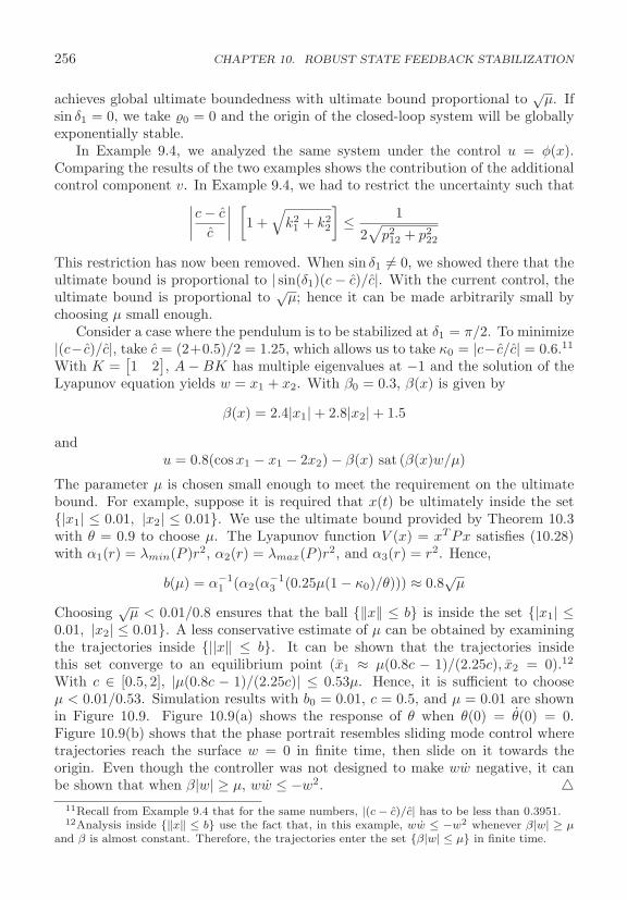
256 CHAPTER 10. ROBUST STATE FEEDBACK STABILIZATION
achieves global ultimate boundedness with ultimate bound proportional to√
μ. Ifsin δ1 = 0, we take �0 = 0 and the origin of the closed-loop system will be globallyexponentially stable.
In Example 9.4, we analyzed the same system under the control u = φ(x).Comparing the results of the two examples shows the contribution of the additionalcontrol component v. In Example 9.4, we had to restrict the uncertainty such that∣∣∣∣c − c
c
∣∣∣∣[1 +√
k21 + k2
2
]≤ 1
2√
p212 + p2
22
This restriction has now been removed. When sin δ1 �= 0, we showed there that theultimate bound is proportional to | sin(δ1)(c − c)/c|. With the current control, theultimate bound is proportional to
√μ; hence it can be made arbitrarily small by
choosing μ small enough.Consider a case where the pendulum is to be stabilized at δ1 = π/2. To minimize
|(c− c)/c|, take c = (2+0.5)/2 = 1.25, which allows us to take κ0 = |c− c/c| = 0.6.11
With K =[1 2
], A − BK has multiple eigenvalues at −1 and the solution of the
Lyapunov equation yields w = x1 + x2. With β0 = 0.3, β(x) is given by
β(x) = 2.4|x1| + 2.8|x2| + 1.5
andu = 0.8(cos x1 − x1 − 2x2) − β(x) sat (β(x)w/μ)
The parameter μ is chosen small enough to meet the requirement on the ultimatebound. For example, suppose it is required that x(t) be ultimately inside the set{|x1| ≤ 0.01, |x2| ≤ 0.01}. We use the ultimate bound provided by Theorem 10.3with θ = 0.9 to choose μ. The Lyapunov function V (x) = xT Px satisfies (10.28)with α1(r) = λmin(P )r2, α2(r) = λmax(P )r2, and α3(r) = r2. Hence,
b(μ) = α−11 (α2(α−1
3 (0.25μ(1 − κ0)/θ))) ≈ 0.8√
μ
Choosing√
μ < 0.01/0.8 ensures that the ball {‖x‖ ≤ b} is inside the set {|x1| ≤0.01, |x2| ≤ 0.01}. A less conservative estimate of μ can be obtained by examiningthe trajectories inside {||x‖ ≤ b}. It can be shown that the trajectories insidethis set converge to an equilibrium point (x1 ≈ μ(0.8c − 1)/(2.25c), x2 = 0).12
With c ∈ [0.5, 2], |μ(0.8c − 1)/(2.25c)| ≤ 0.53μ. Hence, it is sufficient to chooseμ < 0.01/0.53. Simulation results with b0 = 0.01, c = 0.5, and μ = 0.01 are shownin Figure 10.9. Figure 10.9(a) shows the response of θ when θ(0) = θ(0) = 0.Figure 10.9(b) shows that the phase portrait resembles sliding mode control wheretrajectories reach the surface w = 0 in finite time, then slide on it towards theorigin. Even though the controller was not designed to make ww negative, it canbe shown that when β|w| ≥ μ, ww ≤ −w2. �
11Recall from Example 9.4 that for the same numbers, |(c − c)/c| has to be less than 0.3951.12Analysis inside {‖x‖ ≤ b} use the fact that, in this example, ww ≤ −w2 whenever β|w| ≥ μ
and β is almost constant. Therefore, the trajectories enter the set {β|w| ≤ μ} in finite time.
10.3. HIGH-GAIN FEEDBACK 257
0 2 4 60
0.5
1
1.5
−3 −2 −1 0 1 2 3−3
−2
−1
0
1
2
3
Time
θ
(a) (b)
x 1
x2
π/2
Figure 10.9: Simulation results for Example 10.5.
10.3 High-Gain Feedback
High-gain feedback is a classical tool for stabilization and disturbance rejection inthe face of model uncertainty. Both the sliding mode controller of Section 10.1and the Lyapunov redesign controller of Section 10.2 can be replaced by high-gainfeedback controllers.
Starting with sliding mode control, suppose all the assumptions of Theorem 10.1are satisfied. Replace the control v = −β(x) Sat(s/μ) of (10.13) by
v = − β(x)sμ
(10.31)
The derivative of V = 12sT s satisfies
V = − β(x)μ
sT G(x)s + sT Δ(t, x, v)
≤ − β(x)μ
λmin(G(x))‖s‖2 + λmin(G(x))�(x)‖s‖ + λmin(G(x))κ0β(x)
μ‖s‖2
= λmin(G(x))[−(‖s‖
μ− 1)
β(x)(1 − κ0)‖s‖ − β0(1 − κ0)‖s‖]
≤ −λ0β0(1 − κ0)‖s‖, for ‖s‖ ≥ μ
Hence, the trajectories reach the boundary layer {‖s‖ ≤ μ} in finite time. Fromthis point on, the analysis is identical to sliding mode control because inside theboundary layer Sat(s/μ) = s/μ. It follows that Theorems 10.1 and 10.2 hold forthe high-gain feedback control (10.31).
258 CHAPTER 10. ROBUST STATE FEEDBACK STABILIZATION
It is interesting to compare sliding mode control with high-gain feedback. Forconvenience, we limit our comparison to single-input systems and to the case whenboth controllers have ψ = 0. Both the sliding mode control u = −β(x) sat(s/μ) andthe high-gain feedback control u = −β(x)s/μ drive the trajectory to the boundarylayer {|s| ≤ μ} and maintains it there, but the high-gain feedback does it fasterbecause the s equation takes the form
μs = −G(x)s + μΔ
The appearance of μ on the left-hand side shows that, for small μ, s will moverapidly towards the boundary layer. This fast motion towards the boundary layercomes at the expense of a large spike in the control signal in the initial transient.This is different than sliding mode control where |u| ≤ β. Reducing the steady-stateerror when u = −β sat(s/μ) can be achieved by decreasing μ without increasingthe control magnitude, while in the control u = −βs/μ, decreasing the steady-stateerror by decreasing μ results in a large initial spike in the control. These differencesare illustrated in the next example. We note that in the special case when β isconstant, the sliding mode control u = −β sat(s/μ) can be viewed as saturatedhigh-gain feedback control, where the linear feedback −(β/μ)s passes through asaturation function that saturates at ±β.
Example 10.6 In Example 10.1 we designed the sliding mode controller
u = −(2.5 + 2|θ|) sat(s/μ)
where s = θ − π/2 + θ, to practically stabilize the pendulum at θ = π/2. Thecorresponding high-gain feedback controller is
u = −(2.5 + 2|θ|)(s/μ)
Figure 10.10 compares the performance of the two controllers when b = 0.01, c =0.5, and μ = 0.1. Figure 10.10(a) demonstrates that s moves faster towards theboundary layer under high-gain feedback. Figure 10.10(c) shows the spike in thecontrol signal under high-gain feedback, compared with the control signal undersliding mode control, which is shown in Figure 10.10(b). �
Turning now to Lyapunov redesign, suppose all the assumptions of Theorem 10.3are satisfied and replace v = −β(x) Sat(β(x)w/μ) by
v = −β2(x)wμ
(10.32)
This control is used in Section 10.2 when β(x)‖w‖ ≤ μ where it is shown that Vsatisfies (10.27). The only difference here is that (10.32) is used for all w. Therefore,(10.27) is still satisfied and Theorems 10.3 and 10.4 hold for the high-gain feedbackcontrol (10.32).
10.4. EXERCISES 259
0 0.5 1
−1.5
−1
−0.5
0
0 2 4−2
−1
0
1
2
3
4
5
0 0.2 0.4
0
10
20
30
40
Time Time Time
(a) (b) (c)
s n n
Figure 10.10: Comparison of the sliding mode controller u = −(2.5 + 2|θ|) sat(s/0.1)(solid line) with the high-gain feedback controller u = −(2.5 + 2|θ|)(s/0.1) (dashedline) for the pendulum equation of Example 10.6 when θ(0) = θ(0) = 0.
10.4 Exercises
10.1 For each of the following systems, use sliding mode control to design a locallyLipschitz, globally stabilizing state feedback controller. The constants θ1, θ2, andthe function q(t) satisfy the bounds 0 ≤ θ1 ≤ a, 0 < b ≤ θ2 ≤ c, and |q(t)| ≤ d, forknown constants a, b, c, d. You need to verify that the controller will be stabilizingfor μ < μ∗ for some μ∗ > 0 but you do not need to estimate μ∗.
(1) x1 = x2 + 2 sin x1, x2 = θ1x21 + θ2u
(2) x1 = x2 + sin x1, x2 = θ1x1x2 + u
(3) x1 = (1 + x21)x2, x2 = x1 + θ2u
(4) x1 = x21 + x2, x2 = θ1h(x) + u, |h(x)| ≤ ‖x‖
(5) x1 = x31 + x2, x2 = q(t)x3 + u, x3 = x1 − x3
(6) x1 = x1 − θ2u, x2 = 2x2 + θ2u
10.2 For each of the following systems, use sliding mode control to design a locallyLipschitz state feedback controller that ensures global ultimate boundedness withx(t) ultimately in the set {|x1| ≤ δ1, |x2| ≤ δ1} for a given δ1 > 0. The constantsθ1, θ2, and the function q(t) satisfy the bounds 0 ≤ θ1 ≤ a, 0 < b ≤ θ2 ≤ c, and|q(t)| ≤ d, for known constants a, b, c, d. You need to choose μ in terms of δ1.
(1) x1 = x1x2, x2 = x1 + θ2u
260 CHAPTER 10. ROBUST STATE FEEDBACK STABILIZATION
(2) x1 = x2, x2 = sinx1 + u + q(t)
(3) x1 = sin x1 + x2, x2 = u + q(t)
(4) x1 = x1 − θ2u + q(t), x2 = 2x2 + θ2u − q(t)
(5) x1 = −x1 + tanh(x2), x2 = x2 + x3, x3 = u + q(t)
(6) x1 = −x1 + tanh(x2), x2 = θ1x2 + u1, x3 = u2 + q(t)
10.3 Repeat Exercise 10.1 using Lyapunov redesign.
10.4 Repeat Exercise 10.2 using Lyapunov redesign.
10.5 A normalized model of a pendulum whose suspension point is subjected toa time-varying bounded horizontal acceleration is given by
x1 = x2, x2 = − sin x1 − bx2 + cu + h(t)
where b ∈ [0, 0.4], c ∈ [0.5, 1.5], and |h(t)| ≤ 1. It is required to design locallyLipschitz state feedback controller such that, for any initial state, x(t) ∈ {|x1| ≤0.01, |x2| ≤ 0.01} for all t ≥ T for some finite time T . Design the controller using
(a) sliding mode control; (b) Lyapunov redesign; (c) high-gain feedback
10.6 Consider the magnetic levitation system (A.29) with uncertain parametersb ∈ [0, 0.1] and c ∈ [0.8, 1.2]. It is required to regulate x1 to r ∈ [0.5, 1.5], whilemeeting the constraint u ∈ [−2, 0]. The steady-state regulation error should satisfy|x1 − r| ≤ 0.01. Design a locally Lipschitz state feedback controller using
(a) sliding mode control; (b) Lyapunov redesign
10.7 Consider the magnetic levitation system (A.30)–(A.32) with α = 1.5, β = 2and uncertain parameters b ∈ [0, 0.1] and c ∈ [0.8, 1.2]. It is required to regulatex1 to 1 with steady-state error |x1 − 1| ≤ 0.01. Design a locally Lipschitz statefeedback controller. Hint: Transform the system into the controller form using thenominal parameters b = 0 and c = 1.
10.8 Consider the biochemical reactor (A.19) with uncertain ν(x2), but with aknown upper bound νmax such that ν(x2) ≤ νmax over the domain of interest. It isdesired to design a state feedback controller to stabilize the system at x = col(1, 1).
(a) Show that the change of variables η = (x2 − α)/x1, ξ = x2, which is valid inthe region x1 > 0, transforms the system into the regular form.
(b) Let α = 23 and νmax = 1.5. Using sliding mode control, design a controller ofthe form u = −k sat((x2−1)/μ), with positive constants k and μ, such that thesystem is stabilized at an equilibrium point that is O(μ) close to x = col(1, 1),with a region of attraction that includes the set {0.1 ≤ x1 ≤ 2, 0 ≤ x2 ≤ 2}.

10.4. EXERCISES 261
(c) Construct the phase portrait of the closed-loop system in the region {x1 ≥0, x2 ≥ 0} with ν(x2) defined by (A.20), α = 23, β = 0.39, γ = 0.57, andμ = 0.01. For comparison, construct also the phase portrait when u = 1.
10.9 Consider the electrostatic microactuator (A.33) with uncertain ζ ∈ (0, 0.5]and T ∈ [0.1, 0.5]. Using sliding mode control, design a locally Lipschitz statefeedback controller to stabilize the plate at x1 = r, where r ∈ [0.1, 0.9]. Simulatethe closed-loop system with r = 0.5, ζ = 0.1 and T = 0.2. Verify that the controllerachieves stabilization, not only ultimate boundedness.
10.10 Consider the inverted pendulum (A.47) with uncertain a ∈ [0.5, 1.5]. Usingsliding mode control, design a locally Lipschitz state feedback controller to stabilizethe pendulum at θ = 0. Use simulation with a = 1 to find the largest |x1(0)|, whenx(0) = col(x1(0), 0), for which the pendulum is stabilized.
10.11 A simplified model of an underwater vehicle in yaw is given by [39]
ψ + aψ|ψ| = u
where ψ is the heading angle, u is a normalized torque, and a ∈ [0.5, 1.5] is aparameter. Using sliding mode control, design a locally Lipschitz state feedbackcontroller to globally stabilize the system at the equilibrium point (ψ = ψr, ψ = 0).
10.12 Consider the robot manipulator (A.34) and let M , C and g be nominalmodels of M , C, and g, respectively. For the purpose of sliding mode control, takes = Λ(q − qr) + q, where qr is the desired set point and Λ = ΛT > 0.
(a) Show that sliding mode control that achieves global practical stabilization forsufficiently small μ can be taken as
u = −β(x) Sat(s/μ) or u = Cq + g − MΛq − β(x) Sat(s/μ)
and choose β in each case. Are there conditions under which either controlcan achieve stabilization?
(b) Apply both controllers to the two-link manipulator defined by (A.36) and(A.37) with nominal data (A.38) and actual data (A.39). It is desired toregulate the manipulator to qr = (π/2, π/2) under the control constraints|u1| ≤ 6000 and |u2| ≤ 5000. Compare the performance of the two controllers.
10.13 Consider the TORA system (A.49)–(A.52). In this exercise, we design asliding mode controller13 to stabilize the origin.
13The design uses ideas from the passivity-based design of [121].

262 CHAPTER 10. ROBUST STATE FEEDBACK STABILIZATION
(a) Show that
η1 = x1, η2 = x3, η3 = x4 +mLx2 cos x1
m + M, ξ = x2
is a global diffeomorphism that transforms the system into the regular form
η1 = ξ, η2 =−mLξ cos η1
m + M+ η3, η3 =
−kη2
m + M
ξ =1
Δ(η1)[(m + M)u − mL cos η1(mLξ2 sin η1 − kη2)
](b) Show that the derivative of
V0(η) = 12
[k1η
21 +
(m + M)k2
mLη22 +
(m + M)2k2
mLkη23
]with positive constants k1 and k2, is given by V0 = −φ(η)ξ, where φ(η) =−k1η1 + k2η2 cos η1.
(c) Verify that with ξ = φ(η), the origin η = 0 of the η-equation is globally asymp-totically stable and locally exponentially stable.
(d) In view of (c), take
s = ξ − φ(η) = ξ + k1η1 − k2η2 cos η1 = x2 + k1x1 − k2x3 cos x1
Note that s is independent of the system parameters. Choose β(x) such thatu = −β(x) sat(s/μ) globally stabilizes the origin for sufficiently small μ.
10.14 Simulate the TORA system (A.49)–(A.52) with the (A.53) data to comparethe passivity-based control of Exercise 9.13 with the sliding mode control of theprevious exercise. In this comparison, the functions φ1 and φ2 of Exercise 9.13 aretaken as φi(y) = Ui sat(kiy) so that u = −U1 sat(k1x1)−U2 sat(k2x2). The slidingmode control u = −β sat(s/μ) is taken with constant β. Therefore, it only achievesregional stabilization versus global stabilization for the passivity-based control. Thecomparison will be conducted for initial states in the region of attraction of thesliding mode control. We limit both controllers by the control constraint |u| ≤ 0.1,which is met by taking β = 0.1 and U1 + U2 = 0.1.
(a) With initial state x(0) = (π, 0, 0.025, 0), tune the parameters k1, k2, U1, andU2 of the passivity-based control to make the settling time as small as youcan. You should be able to achieve a settling time of about 30 sec.
(b) With initial state x(0) = (π, 0, 0.025, 0), tune the parameters k1, k2, and μ ofthe sliding mode control to make the settling time as small as you can. Youshould be able to achieve a settling time of about 4 sec.
(c) Compare the performance of the two controllers.
Chapter 11
Nonlinear Observers
In this chapter we study the design of observers to estimate the state x of thenonlinear system
x = f(x, u), y = h(x)
where u is a given input and y is the measured output. The observers will take thegeneral form
˙x = f(x, u) + H(·)[y − h(x)]
where the observer gain H(·) could be a constant or time-varying matrix. The termf(x, u) in the observer equation is a prediction term that duplicates the dynamicsof the system, while H[y − h(x)] is a correction term1 that depends on the error inestimating the output y by h(x). For the linear system
x = Ax + Bu, y = Cx
the estimation error x = x − x satisfies the linear equation
˙x = (A − HC)x
If the pair (A,C) is detectable, that is, observable or having unobservable eigenval-ues with negative real parts, the matrix H can be designed such that A − HC isHurwitz, which implies that limt→∞ x(t) = 0; hence, the estimate x(t) asymptoti-cally approaches x(t) as t tends to infinity. For nonlinear systems, we present differ-ent approaches to the design of nonlinear observers. The first two sections presentapproaches that are based on linearization. The local observer of Section 11.1 is de-signed by linearization about an equilibrium point of the system x = f(x, u); henceit is guaranteed to work only when x and u are sufficiently close to their equilibriumvalues, in addition to requiring ‖x(0)‖ to be sufficiently small. The observer of Sec-tion 11.2 is a deterministic version of the Extended Kalman Filter from nonlinear
1Or innovation term in the language of estimation theory.
263

264 CHAPTER 11. NONLINEAR OBSERVERS
estimation theory.2 Here linearization is taken about the estimate x; therefore, theobserver gain is time varying and has to be calculated in real time since H(t) atany time t depends on x(t). The observer still requires the initial estimation error‖x(0)‖ to be sufficiently small, but now x(t) and u(t) can be any well-defined trajec-tories that have no finite escape time. The observer of Section 11.3 is developed fornonlinear systems in the observer form of Section 8.3 and has linear error dynamicsidentical to the case of linear observers. Hence, convergence of the estimation errorx is global; that is, limt→∞ x(t) = 0 for all initial conditions x(0). It is also shownthat the same design will work for a more general system that has an additionalLipschitz nonlinearity provided the Lipschitz constant is sufficiently small.3
The observers of the first three sections assume perfect knowledge of the non-linear functions f and h. Because, in all three cases, we will show that the errordynamics have an exponentially stable origin, we can see from the robustness anal-ysis of Section 4.3 that for sufficiently small bounded perturbations of f or h, theestimation error x(t) will be ultimately bounded by a small upper bound. How-ever, there is no guarantee that these observers will function in the presence oflarge perturbations. The high-gain observer of Section 11.4 applies to a specialclass of nonlinear systems, but can be designed to be robust to a certain level ofuncertainty that cannot be tolerated in the observers of Section 11.1 to 11.3. Therobustness is achieved by designing the observer gain high enough, which makes theestimation-error dynamics much faster than those of the system x = f(x, u). Thefast dynamics play an important role when the observer is used in feedback control,as we shall see in Section 12.4.
11.1 Local Observers
Consider the nonlinear system
x = f(x, u), y = h(x) (11.1)
together with the observer
˙x = f(x, u) + H[y − h(x)] (11.2)
where x ∈ Rn, u ∈ Rm, y ∈ Rp, f and h are twice continuously differentiable intheir arguments, and H is an n×p constant matrix. The estimation error x = x− xsatisfies the equation
˙x = f(x, u) − f(x, u) − H[h(x) − h(x)] (11.3)
Equation (11.3) has an equilibrium point at x = 0 and our goal is to design theobserver gain H to make this equilibrium point exponentially stable. We seek a
2See [47] or [127].3See [5, 46, 72, 123] for more approaches to nonlinear observers.
11.1. LOCAL OBSERVERS 265
local solution for sufficiently small ‖x(0)‖. Linearization of (11.3) at x = 0 resultsin the linear time-varying system
˙x =[∂f
∂x(x(t), u(t)) − H
∂h
∂x(x(t))
]x (11.4)
Designing a constant matrix H to stabilize the origin of the foregoing time-varyingsystem is almost impossible, especially in view of the fact that it should work forall initial states x(0) and all inputs u(t) in a certain domain. We assume that thereare vectors xss ∈ Rn and uss ∈ Rm such that the system (11.1) has an equilibriumpoint x = xss when u = uss and that the output y = 0 at equilibrium; that is,
0 = f(xss, uss), 0 = h(xss)
Furthermore, we assume that given ε > 0, there exist δ1 > 0 and δ2 > 0 such that
‖x(0) − xss‖ ≤ δ1 and ‖u(t) − uss‖ ≤ δ2 ∀ t ≥ 0
ensure that x(t) is defined for all t ≥ 0 and satisfies ‖x(t) − xss‖ ≤ ε for all t ≥ 0.Let
A =∂f
∂x(xss, uss), C =
∂h
∂x(xss)
and assume that the pair (A,C) is detectable. Design H such that A − HC isHurwitz.
Lemma 11.1 For sufficiently small ‖x(0)‖, ‖x(0)− xss‖, and supt≥0 ‖u(t)− uss‖,
limt→∞ x(t) = 0
�
Proof: By (B.6), we have
f(x, u) − f(x, u) =∫ 1
0
∂f
∂x(x − σx, u) dσ x
Hence,
‖f(x, u) − f(x, u) − Ax‖ =∥∥∥∥∫ 1
0
[∂f
∂x(x − σx, u) − ∂f
∂x(x, u) +
∂f
∂x(x, u) − ∂f
∂x(xss, uss)
]dσ x
∥∥∥∥≤ L1( 1
2‖x‖ + ‖x − xss‖ + ‖u − uss‖)‖x‖
where L1 is a Lipschitz constant of [∂f/∂x]. Similarly, it can be shown that
‖h(x) − h(x) − Cx‖ ≤ L2( 12‖x‖ + ‖x − xss‖)‖x‖
266 CHAPTER 11. NONLINEAR OBSERVERS
where L2 is a Lipschitz constant of [∂h/∂x]. Therefore, the estimation-error dy-namics can be written as
˙x = (A − HC)x + Δ(x, u, x) (11.5)
where‖Δ(x, u, x)‖ ≤ k1‖x‖2 + k2(ε + δ2)‖x‖
for some positive constants k1 and k2. Let V = xT P x, where P is the positivedefinite solution of the Lyapunov equation P (A−HC)+(A−HC)T P = −I. UsingV as a Lyapunov function candidate for (11.5), we obtain
V ≤ −‖x‖2 + c4k1‖x‖3 + c4k2(ε + δ2)‖x‖2
where c4 = 2‖P‖. Thus
V ≤ −13‖x‖2, for c4k1‖x‖ ≤ 1
3 and c4k2(ε + δ2) ≤ 13
which shows that for sufficiently small ‖x(0)‖, ε, and δ2, the estimation error con-verges to zero as t tends to infinity. Smallness of ε can be ensured by choosing δ1
and δ2 sufficiently small. �
11.2 The Extended Kalman Filter
Consider the nonlinear system
x = f(x, u), y = h(x) (11.6)
where x ∈ Rn, u ∈ Rm, y ∈ Rp, f and h are twice continuously differentiable intheir arguments, and x(t) and u(t) are bounded for all t ≥ 0. Consider the observer
˙x = f(x, u) + H(t)[y − h(x)] (11.7)
with time-varying observer gain H(t). The estimation error x = x − x satisfies theequation
˙x = f(x, u) − f(x, u) − H(t)[h(x) − h(x)] (11.8)
Expanding the right-hand side in a Taylor series about x = 0 and evaluating theJacobian matrices along x, the foregoing equation can be written as
˙x = [A(t) − H(t)C(t)]x + Δ(x, x, u) (11.9)
whereA(t) =
∂f
∂x(x(t), u(t)), C(t) =
∂h
∂x(x(t)) (11.10)
andΔ = f(x, u) − f(x, u) − A(t)x − H(t) [h(x) − h(x) − C(t)x]
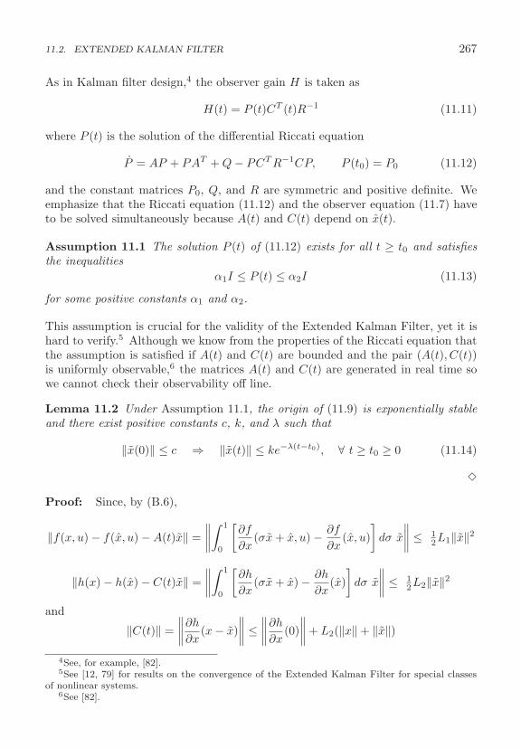
11.2. EXTENDED KALMAN FILTER 267
As in Kalman filter design,4 the observer gain H is taken as
H(t) = P (t)CT (t)R−1 (11.11)
where P (t) is the solution of the differential Riccati equation
P = AP + PAT + Q − PCT R−1CP, P (t0) = P0 (11.12)
and the constant matrices P0, Q, and R are symmetric and positive definite. Weemphasize that the Riccati equation (11.12) and the observer equation (11.7) haveto be solved simultaneously because A(t) and C(t) depend on x(t).
Assumption 11.1 The solution P (t) of (11.12) exists for all t ≥ t0 and satisfiesthe inequalities
α1I ≤ P (t) ≤ α2I (11.13)
for some positive constants α1 and α2.
This assumption is crucial for the validity of the Extended Kalman Filter, yet it ishard to verify.5 Although we know from the properties of the Riccati equation thatthe assumption is satisfied if A(t) and C(t) are bounded and the pair (A(t), C(t))is uniformly observable,6 the matrices A(t) and C(t) are generated in real time sowe cannot check their observability off line.
Lemma 11.2 Under Assumption 11.1, the origin of (11.9) is exponentially stableand there exist positive constants c, k, and λ such that
‖x(0)‖ ≤ c ⇒ ‖x(t)‖ ≤ ke−λ(t−t0), ∀ t ≥ t0 ≥ 0 (11.14)
�
Proof: Since, by (B.6),
‖f(x, u) − f(x, u) − A(t)x‖ =∥∥∥∥∫ 1
0
[∂f
∂x(σx + x, u) − ∂f
∂x(x, u)
]dσ x
∥∥∥∥ ≤ 12L1‖x‖2
‖h(x) − h(x) − C(t)x‖ =∥∥∥∥∫ 1
0
[∂h
∂x(σx + x) − ∂h
∂x(x)]
dσ x
∥∥∥∥ ≤ 12L2‖x‖2
and
‖C(t)‖ =∥∥∥∥∂h
∂x(x − x)
∥∥∥∥ ≤∥∥∥∥∂h
∂x(0)∥∥∥∥+ L2(‖x‖ + ‖x‖)
4See, for example, [82].5See [12, 79] for results on the convergence of the Extended Kalman Filter for special classes
of nonlinear systems.6See [82].
268 CHAPTER 11. NONLINEAR OBSERVERS
where L1 and L2 are Lipschitz constants of [∂f/∂x] and [∂h/∂x], respectively, thereexist positive constants k1 and k2 such that ‖Δ(x, x, u)‖ ≤ k1‖x‖2 + k3‖x‖3. Itfollows from Assumption 11.1 that P−1(t) exists for all t ≥ t0 and satisfies
α3I ≤ P−1(t) ≤ α4I (11.15)
for some positive constants α3 and α4. Using V = xT P−1x as a Lyapunov functioncandidate for (11.9) and noting that dP−1/dt = −P−1PP−1, we have
V = xT P−1 ˙x + ˙xT P−1x + xT d
dtP−1x
= xT P−1(A − PCT R−1C)x + xT (AT − CT R−1CP )P−1x
− xT P−1PP−1x + 2xT P−1Δ= xT P−1(AP + PAT − PCT R−1CP − P )P−1x − xT CT R−1Cx + 2xT P−1Δ
Substitution of P using (11.12) results in
V = −xT (P−1QP−1 + CT R−1C)x + 2xT P−1Δ
The matrix P−1QP−1 is positive definite uniformly in t, in view of (11.15), andthe matrix CT R−1C is positive semidefinite. Hence their sum is positive definiteuniformly in t. Thus, V satisfies the inequality
V ≤ −c1‖x‖2 + c2k1‖x||3 + c2k2‖x||4
for some positive constants c1 and c2. Consequently,
V ≤ −12c1‖x‖2, for ‖x‖ ≤ r
where r is the positive root of − 12c1 + c2k1y + c2k2y
2. The foregoing inequalityshows that the origin is exponentially stable and completes the proof. �
Example 11.1 Consider the system
x = A1x + B1[0.25x21x2 + 0.2 sin 2t], y = C1x
where
A1 =[
0 1−1 −2
], B1 =
[01
], C1 =
[1 0
]We start by investigating boundedness of x(t). Taking V1(x) = xT P1x, where
P1 = 12
[3 11 1
]is the solution of the Lyapunov equation P1A1 + AT
1 P1 = −I, it can
be shown that
V1 = −xT x + 2xT P1B1[0.25x21x2 + 0.2 sin 2t]
≤ −‖x‖2 + 0.5‖P1B1‖x21‖x‖2 + 0.4‖P1B1‖‖x‖
= −‖x‖2 +x2
1
2√
2‖x‖2 +
0.4√2‖x‖ ≤ −0.5‖x‖2 +
0.4√2‖x‖

11.3. GLOBAL OBSERVERS 269
for x21 ≤ √
2. Noting that minx21=
√2 xT Px =
√2/(bT P−1b) =
√2, where b =
col(1, 0),7 we see that Ω = {V1(x) ≤ √2} ⊂ {x2
1 ≤ √2}. Inside Ω, we have
V1 ≤ −0.5‖x‖2 +0.4√
2‖x‖ ≤ −0.15‖x‖2, ∀ ‖x‖ ≥ 0.4
0.35√
2= 0.8081
With λmax(P1) = 1.7071, we have (0.8081)2λmax(P1) <√
2. Hence the ball {‖x‖ ≤0.8081} is in the interior of Ω. This shows that V is negative on the boundary∂Ω. Therefore, Ω is positively invariant and x(t) is bounded for all x(0) ∈ Ω. Wewill now design an Extended Kalman Filter to estimate x(t) for x(0) ∈ Ω. TakingQ = R = P (0) = I, the Riccati equation (11.12) is given by
P = AP + PAT + I − PCT CP, P (0) = I
where
A(t) =[
0 1−1 + 0.5x1(t)x2(t) −2 + 0.25x2
1(t)
]and C =
[1 0
]Taking P =
[p11 p12
p12 p22
], it can be shown that the Extended Kalman Filter is defined
by the five simultaneous equations:
˙x1 = x2 + p11(y − x1)˙x2 = −x1 − 2x2 + 0.25x2
1x2 + 0.2 sin 2t + p12(y − x1)p11 = 2p12 + 1 − p2
11
p12 = p11(−1 + 0.5x1x2) + p12(−2 + 0.25x21) + p22 − p11p12
p22 = 2p12(−1 + 0.5x1x2) + 2p22(−2 + 0.25x21) + 1 − p2
12
with initial conditions x1(0), x2(0), p11(0) = 1, p12(0) = 0, and p22(0) = 1. Fig-ure 11.1 shows simulation results for x1(0) = 1, x2(0) = −1, x1(0) = x2(0) = 0. Wenote that the estimation error converges to zero for a relatively large initial error.
�
11.3 Global Observers
Consider a nonlinear system in the observer form
x = Ax + ψ(u, y), y = Cx (11.16)
where x ∈ Rn, u ∈ Rm, y ∈ Rp, (A,C) is observable, ψ is locally Lipschitz, andx(t) and u(t) are defined for all t ≥ 0. The observer for (11.16) is taken as
˙x = Ax + ψ(u, y) + H(y − Cx) (11.17)7See (B.3).
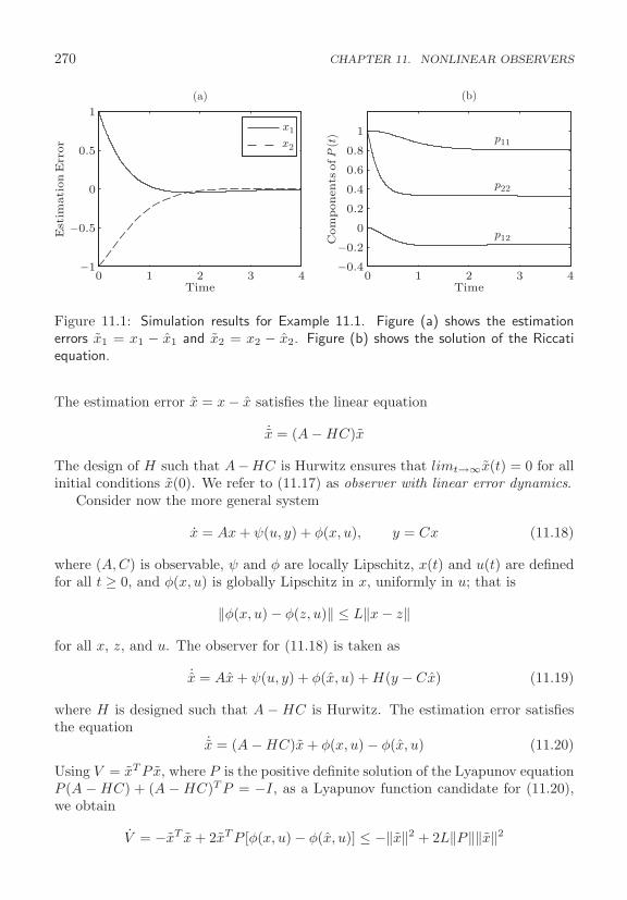
270 CHAPTER 11. NONLINEAR OBSERVERS
0 1 2 3 4−1
−0.5
0
0.5
1
Est
imati
on
Err
or
0 1 2 3 4−0.4
−0.2
0
0.2
0.4
0.6
0.8
1
Com
ponents
of P
(t)
TimeTime
x2p11
p22
p12
x1
(a) (b)
Figure 11.1: Simulation results for Example 11.1. Figure (a) shows the estimationerrors x1 = x1 − x1 and x2 = x2 − x2. Figure (b) shows the solution of the Riccatiequation.
The estimation error x = x − x satisfies the linear equation
˙x = (A − HC)x
The design of H such that A−HC is Hurwitz ensures that limt→∞x(t) = 0 for allinitial conditions x(0). We refer to (11.17) as observer with linear error dynamics.
Consider now the more general system
x = Ax + ψ(u, y) + φ(x, u), y = Cx (11.18)
where (A,C) is observable, ψ and φ are locally Lipschitz, x(t) and u(t) are definedfor all t ≥ 0, and φ(x, u) is globally Lipschitz in x, uniformly in u; that is
‖φ(x, u) − φ(z, u)‖ ≤ L‖x − z‖
for all x, z, and u. The observer for (11.18) is taken as
˙x = Ax + ψ(u, y) + φ(x, u) + H(y − Cx) (11.19)
where H is designed such that A − HC is Hurwitz. The estimation error satisfiesthe equation
˙x = (A − HC)x + φ(x, u) − φ(x, u) (11.20)
Using V = xT P x, where P is the positive definite solution of the Lyapunov equationP (A − HC) + (A − HC)T P = −I, as a Lyapunov function candidate for (11.20),we obtain
V = −xT x + 2xT P [φ(x, u) − φ(x, u)] ≤ −‖x‖2 + 2L‖P‖‖x‖2
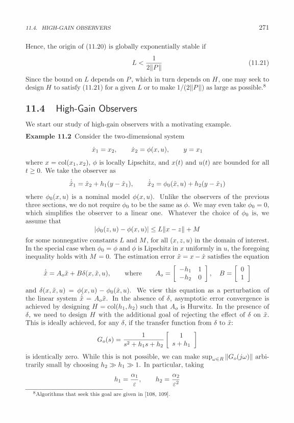
11.4. HIGH-GAIN OBSERVERS 271
Hence, the origin of (11.20) is globally exponentially stable if
L <1
2‖P‖ (11.21)
Since the bound on L depends on P , which in turn depends on H, one may seek todesign H to satisfy (11.21) for a given L or to make 1/(2‖P‖) as large as possible.8
11.4 High-Gain Observers
We start our study of high-gain observers with a motivating example.
Example 11.2 Consider the two-dimensional system
x1 = x2, x2 = φ(x, u), y = x1
where x = col(x1, x2), φ is locally Lipschitz, and x(t) and u(t) are bounded for allt ≥ 0. We take the observer as
˙x1 = x2 + h1(y − x1), ˙x2 = φ0(x, u) + h2(y − x1)
where φ0(x, u) is a nominal model φ(x, u). Unlike the observers of the previousthree sections, we do not require φ0 to be the same as φ. We may even take φ0 = 0,which simplifies the observer to a linear one. Whatever the choice of φ0 is, weassume that
|φ0(z, u) − φ(x, u)| ≤ L‖x − z‖ + M
for some nonnegative constants L and M , for all (x, z, u) in the domain of interest.In the special case when φ0 = φ and φ is Lipschitz in x uniformly in u, the foregoinginequality holds with M = 0. The estimation error x = x− x satisfies the equation
˙x = Aox + Bδ(x, x, u), where Ao =[ −h1 1
−h2 0
], B =
[01
]and δ(x, x, u) = φ(x, u) − φ0(x, u). We view this equation as a perturbation ofthe linear system ˙x = Aox. In the absence of δ, asymptotic error convergence isachieved by designing H = col(h1, h2) such that Ao is Hurwitz. In the presence ofδ, we need to design H with the additional goal of rejecting the effect of δ on x.This is ideally achieved, for any δ, if the transfer function from δ to x:
Go(s) =1
s2 + h1s + h2
[1
s + h1
]is identically zero. While this is not possible, we can make supω∈R ‖Go(jω)‖ arbi-trarily small by choosing h2 � h1 � 1. In particular, taking
h1 =α1
ε, h2 =
α2
ε2
8Algorithms that seek this goal are given in [108, 109].
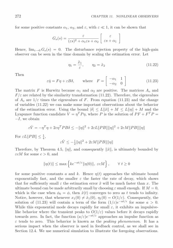
272 CHAPTER 11. NONLINEAR OBSERVERS
for some positive constants α1, α2, and ε, with ε � 1, it can be shown that
Go(s) =ε
(εs)2 + α1εs + α2
[ε
εs + α1
]
Hence, limε→0 Go(s) = 0. The disturbance rejection property of the high-gainobserver can be seen in the time domain by scaling the estimation error. Let
η1 =x1
ε, η2 = x2 (11.22)
Then
εη = Fη + εBδ, where F =[ −α1 1
−α2 0
](11.23)
The matrix F is Hurwitz because α1 and α2 are positive. The matrices Ao andF/ε are related by the similarity transformation (11.22). Therefore, the eigenvaluesof Ao are 1/ε times the eigenvalues of F . From equation (11.23) and the changeof variables (11.22) we can make some important observations about the behaviorof the estimation error. Using the bound |δ| ≤ L‖x‖ + M ≤ L‖η‖ + M and theLyapunov function candidate V = ηT Pη, where P is the solution of PF + FT P =−I, we obtain
εV = −ηT η + 2εηT PBδ ≤ −‖η‖2 + 2εL‖PB‖‖η‖2 + 2εM‖PB‖‖η‖
For εL‖PB‖ ≤ 14 ,
εV ≤ −12‖η‖2 + 2εM‖PB‖‖η‖
Therefore, by Theorem 4.5, ‖η‖, and consequently ‖x‖, is ultimately bounded byεcM for some c > 0, and
‖η(t)‖ ≤ max{
ke−at/ε‖η(0)‖, εcM}
, ∀ t ≥ 0
for some positive constants a and k. Hence η(t) approaches the ultimate boundexponentially fast, and the smaller ε the faster the rate of decay, which showsthat for sufficiently small ε the estimation error x will be much faster than x. Theultimate bound can be made arbitrarily small by choosing ε small enough. If M = 0,which is the case when φ0 = φ, then x(t) converges to zero as t tends to infinity.Notice, however, that whenever x1(0) = x1(0), η1(0) = O(1/ε). Consequently, thesolution of (11.23) will contain a term of the form (1/ε)e−at/ε for some a > 0.While this exponential mode decays rapidly for small ε, it exhibits an impulsive-like behavior where the transient peaks to O(1/ε) values before it decays rapidlytowards zero. In fact, the function (a/ε)e−at/ε approaches an impulse function asε tends to zero. This behavior is known as the peaking phenomenon. It has aserious impact when the observer is used in feedback control, as we shall see inSection 12.4. We use numerical simulation to illustrate the foregoing observations.
11.4. HIGH-GAIN OBSERVERS 273
We saw in Example 11.1 that for all x(0) ∈ Ω = {1.5x21 + x1x2 + 0.5x2
2 ≤ √2}, the
state x(t) of the system
x1 = x2, x2 = −x1 − 2x2 + ax21x2 + b sin 2t, y = x1
with a = 0.25 and b = 0.2, is bounded. We use the high-gain observer
˙x1 = x2 +2ε(y − x1), ˙x2 = −x1 − 2x2 + ax2
1x2 + b sin 2t +1ε2
(y − x1)
with two different choice of the pair (a, b). When a = 0.25 and b = 0.2 are known,we take a = 0.25 and b = 0.2. This is a case with no model uncertainty andφ0 = φ. The other case is when the coefficients a and b are unknown. In thiscase we take a = b = 0. Figure 11.2 shows simulation results for both cases.Figures 11.2(a) and (b) show the state x and its estimate x in the no-uncertaintycase for different values of ε. The estimate x2 illustrates the peaking phenomenon.We note that the peaking phenomenon is not present in x1. While peaking isinduced by the error x1(0) − x1(0), it does not appear in x1 because x1 = εη1.Figures 11.2(c) and (d) show the estimation error x2 for the uncertain model casewhen a = b = 0. Comparison of Figures 11.2(b) and (c) shows that the presence ofuncertainty has very little effect on the performance of the observer. Figure 11.2(d)demonstrates the fact that the ultimate bound on the estimation error is of theorder O(ε). We conclude the example by discussing the effect of measurementnoise on the performance of high-gain observers.9 Suppose the measurement y iscorrupted by bounded measurement noise v; that is, y = x1 + v, and let |v(t)| ≤ N .Equation (11.23) will take the form
εη = Fη + εBδ − 1εEv, where E =
[α1
α2
]
and the inequality satisfied by V changes to
εV ≤ −12‖η‖2 + 2εM‖PB‖‖η‖ +
2N
ε‖PE‖‖η‖
Therefore, the ultimate bound on ‖x‖ takes the form
‖x‖ ≤ c1Mε +c2N
ε(11.24)
for some positive constants c1 and c2. This inequality shows a tradeoff betweenmodel uncertainty and measurement noise. An illustration of the ultimate bound
9Other factors that limit the performance of high-gain observers in digital implementation arethe sampling rate and the computer wordlength. The sampling rate needs to be high enough tocapture the fast changing estimates, and the wordlength should be large enough to represent thevery large (or very small) numbers encountered in the observer. Because of technology advances,these factors are not as important as the effect of measurement noise.
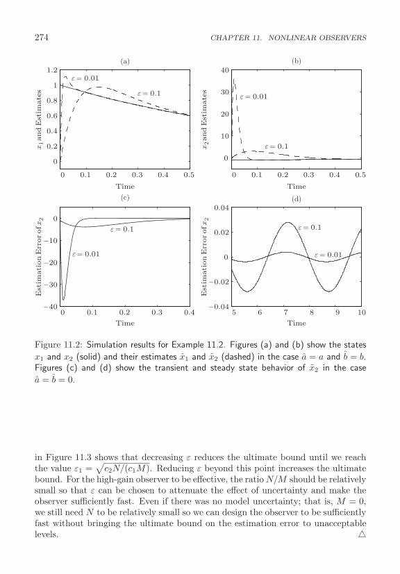
274 CHAPTER 11. NONLINEAR OBSERVERS
0 0.1 0.2 0.3 0.4 0.5 0.1 0.2 0.3 0.4 0.5
0
0.2
0.4
0.6
0.8
1
1.2
x1and
Est
imate
s
x2and
Est
imate
s
0
10
20
30
40
0 0.1 0.2 0.3 0.4−40
−30
−20
−10
0
Est
imati
on
Err
orofx2
Est
imati
on
Err
orofx2
5 6 7 8 9 10−0.04
−0.02
0
0
0.02
0.04
TimeTime
TimeTime
(c)
(a) (b)
(d)
ε = 0.01
ε = 0.01
ε = 0.01
ε = 0.01
ε = 0.1
ε = 0.1
ε = 0.1
ε = 0.1
Figure 11.2: Simulation results for Example 11.2. Figures (a) and (b) show the states
x1 and x2 (solid) and their estimates x1 and x2 (dashed) in the case a = a and b = b.Figures (c) and (d) show the transient and steady state behavior of x2 in the case
a = b = 0.
in Figure 11.3 shows that decreasing ε reduces the ultimate bound until we reachthe value ε1 =
√c2N/(c1M). Reducing ε beyond this point increases the ultimate
bound. For the high-gain observer to be effective, the ratio N/M should be relativelysmall so that ε can be chosen to attenuate the effect of uncertainty and make theobserver sufficiently fast. Even if there was no model uncertainty; that is, M = 0,we still need N to be relatively small so we can design the observer to be sufficientlyfast without bringing the ultimate bound on the estimation error to unacceptablelevels. �
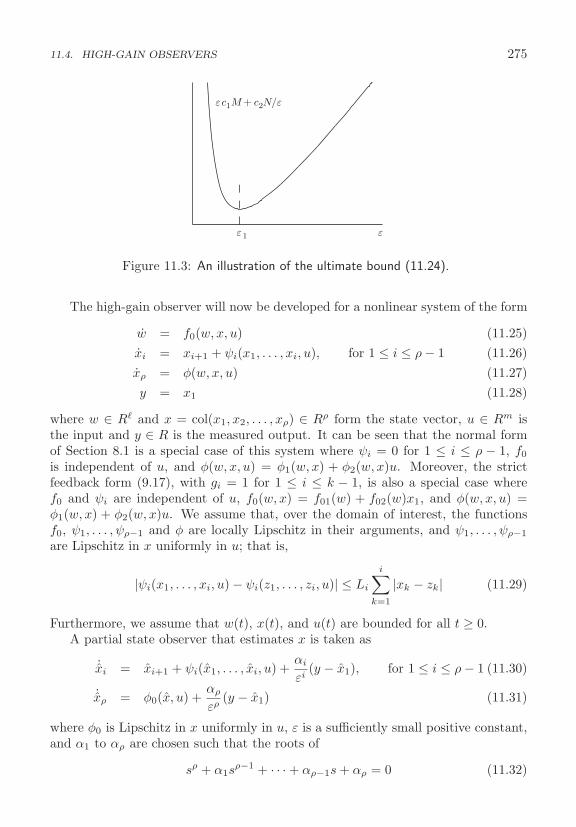
11.4. HIGH-GAIN OBSERVERS 275
ε c1M+ c2N/ε
ε 1 ε
Figure 11.3: An illustration of the ultimate bound (11.24).
The high-gain observer will now be developed for a nonlinear system of the form
w = f0(w, x, u) (11.25)xi = xi+1 + ψi(x1, . . . , xi, u), for 1 ≤ i ≤ ρ − 1 (11.26)xρ = φ(w, x, u) (11.27)y = x1 (11.28)
where w ∈ R� and x = col(x1, x2, . . . , xρ) ∈ Rρ form the state vector, u ∈ Rm isthe input and y ∈ R is the measured output. It can be seen that the normal formof Section 8.1 is a special case of this system where ψi = 0 for 1 ≤ i ≤ ρ − 1, f0
is independent of u, and φ(w, x, u) = φ1(w, x) + φ2(w, x)u. Moreover, the strictfeedback form (9.17), with gi = 1 for 1 ≤ i ≤ k − 1, is also a special case wheref0 and ψi are independent of u, f0(w, x) = f01(w) + f02(w)x1, and φ(w, x, u) =φ1(w, x) + φ2(w, x)u. We assume that, over the domain of interest, the functionsf0, ψ1, . . . , ψρ−1 and φ are locally Lipschitz in their arguments, and ψ1, . . . , ψρ−1
are Lipschitz in x uniformly in u; that is,
|ψi(x1, . . . , xi, u) − ψi(z1, . . . , zi, u)| ≤ Li
i∑k=1
|xk − zk| (11.29)
Furthermore, we assume that w(t), x(t), and u(t) are bounded for all t ≥ 0.A partial state observer that estimates x is taken as
˙xi = xi+1 + ψi(x1, . . . , xi, u) +αi
εi(y − x1), for 1 ≤ i ≤ ρ − 1 (11.30)
˙xρ = φ0(x, u) +αρ
ερ(y − x1) (11.31)
where φ0 is Lipschitz in x uniformly in u, ε is a sufficiently small positive constant,and α1 to αρ are chosen such that the roots of
sρ + α1sρ−1 + · · · + αρ−1s + αρ = 0 (11.32)

276 CHAPTER 11. NONLINEAR OBSERVERS
have negative real parts. The function φ0 in (11.31) is a nominal model of φ. Weassume that
‖φ(w, x, u) − φ0(z, u)‖ ≤ L ‖x − z‖ + M (11.33)
Because
φ(w, x, u) − φ0(z, u) = φ(w, x, u) − φ0(x, u) + φ0(x, u) − φ0(z, u)
and φ0 is Lipschitz, (11.33) requires the modeling error φ(w, x, u) − φ0(x, u) to bebounded.
Lemma 11.3 Under the stated assumptions, there is ε∗ > 0 such that for 0 < ε ≤ε∗, the estimation errors xi = xi − xi, for 1 ≤ i ≤ ρ, of the high-gain observer(11.30)–(11.31) satisfy the bound
|xi| ≤ max{
b
εi−1e−at/ε, ερ+1−icM
}(11.34)
for some positive constants a, b, c. �
Proof: Define the scaled estimation errors
η1 =x1 − x1
ερ−1, η2 =
x2 − x2
ερ−2, . . . , ηρ−1 =
xρ−1 − xρ−1
ε, ηρ = xρ − xρ (11.35)
It can be shown that η = col(η1, η2, · · · , ηρ) satisfies the equation
εη = Fη + εδ(w, x, x, u) (11.36)
where δ = col(δ1, δ2, · · · , δρ),
F =
⎡⎢⎢⎢⎢⎢⎣
−α1 1 0 · · · 0−α2 0 1 · · · 0
.... . .
...−αρ−1 0 1−αρ 0 · · · · · · 0
⎤⎥⎥⎥⎥⎥⎦ , δρ = φ(w, x, u) − φ0(x, u)
and
δi =1
ερ−i[ψi(x1, . . . , xi, u) − ψi(x1, . . . , xi, u)], for 1 ≤ i ≤ ρ − 1
The matrix F is Hurwitz by design because its characteristic equation is (11.32).Using (11.29) we see that δ1 to δρ−1 satisfy
|δi| ≤ Li
ερ−i
i∑k=1
|xk − xk| =Li
ερ−i
i∑k=1
ερ−k|ηk| = Li
i∑k=1
εi−k|ηk|

11.5. EXERCISES 277
The preceding inequality and (11.33) show that
‖δ‖ ≤ Lδ‖η‖ + M (11.37)
where Lδ is independent of ε for all ε ≤ ε∗ for any given ε∗ > 0. Let V = ηT Pη,where P = PT > 0 is the solution of the Lyapunov equation PF + FT P = −I.Then
εV = −ηT η + 2εηT Pδ
Using (11.37) we obtain
εV ≤ −‖η‖2 + 2ε‖P‖Lδ‖η‖2 + 2ε‖P‖M‖η‖For ε‖P‖Lδ ≤ 1
4 ,
εV ≤ −12‖η‖2 + 2ε‖P‖M‖η‖ ≤ −1
4‖η‖2, ∀ ‖η‖ ≥ 8ε‖P‖MWe conclude by Theorem 4.5 that
‖η(t)‖ ≤ max{
ke−at/ε‖η(0)‖, εcM}
, ∀ t ≥ 0
for some positive constants a, c, and k. From (11.35) we see that ‖η(0)‖ ≤ β/ερ−1,for some β > 0, and |xi| ≤ ερ−i|ηi|, which yields (11.34). �
11.5 Exercises
11.1 Consider the van der Pol equation
x1 = x2, x2 = −x1 + (1 − x21)x2, y = x1
(a) Design an Extended Kalman Filter.
(b) Design a high-gain observer with ε = 0.01.
(c) Compare the performance of the two observers using simulation.
11.2 A normalized state model of the Duffing equation (A.4) is given by
x1 = x2, x2 = −x1(1 + x21) − x2 + a cos(t), y = x1
(a) Design an observer with linear error dynamics when a = 1.
(b) Design a high-gain observer with ε = 0.01.
(c) Using simulation, compare the performance of the two observers when a isperturbed. (Keep a = 1 in the observer but gradually increase it in thesystem’s equation.)
278 CHAPTER 11. NONLINEAR OBSERVERS
11.3 The Wien-Bridge oscillator of Exercise 2.5, with C1 = C2 = C and R1 =R2 = R, is modeled in the τ = t/(CR) time scale by the equations
x1 = − 12x2, x2 = 2(x1 − x2) + g(x2) − x2
where g(v) = 3.234v − 2.195v3 + 0.666v5. Suppose the measured output is x2.
(a) Design an Extended Kalman Filter.
(b) Design an observer with linear error dynamics.
(c) Design a high-gain observer with ε = 0.01. Hint: Transform the system intothe form (11.26)–(11.28).
(d) Using simulation, compare the performance of the three observers.
(e) Repeat (d) when g in the system’s equation is perturbed to 1.2g.
11.4 Consider the electrostatic microactuator (A.33) with ζ = 0.1 and T = 0.2.Under the constant input u = 5/(4
√2), the system has an asymptotically stable
equilibrium point at x = col(1/6, 0, 1/√
2). Assume that the measured outputsare x1 and x3. The state x2 can be estimated by one of the following high-gainobservers:
˙x1 = x2 + (α1/ε)(x1 − x1), ˙x2 = −x1 + 13x2
3 + (α2/ε2)(x1 − x1)
or˙x1 = x2 + (α1/ε)(x1 − x1), ˙x2 = −x1 + (α2/ε2)(x1 − x1)
where in the first observer 13x2
3is treated as a given input, while in the second oneit is treated as disturbance. Use simulation to compare the performance of the twoobservers for ε = 1 and 0.1. Let α1 = 2 and α2 = 1. Limit x(0) to the region ofattraction of x.
11.5 Consider the system
x1 = β1(x1) + x2, x2 = β2(x1) + β3(x1)x2 + u, y = x1
where β1 to β3 are smooth functions.
(a) Design an observer with linear error dynamics.
(b) Design a high-gain observer.
(c) Repeat part (b) when the function β2 and β3 are unknown.
11.6 Consider the single link manipulator with flexible joint from Example 8.15.
(a) Design an observer with linear error dynamics when y = x1.

11.5. EXERCISES 279
(b) Design an observer with linear error dynamics when y = col(x1, x3).
(c) Design a high-gain observer when y = x1.
(d) Design a high-gain observer when y = col(x1, x3) and the parameters a, b, c, dare unknown.
11.7 Consider the high-gain observer (11.30)–(11.31) when y(t) = x1(t)+v(t) with|v(t)| ≤ N . Show that the bound (11.34) changes to
|xi| ≤ max{
b
εi−1e−at/ε, ερ+1−icM +
c2N
εi−1
}for some c2 > 0.
11.8 A modified Extended Kalman Filter in which the estimation error decays tozero faster than an exponential ke−αt with a prescribed positive constant α [110]can be obtained by changing the Riccati equation (11.12) to
P = (A + αI)P + P (AT + αI) + Q − PCT R−1CP, P (t0) = P0
Redesign the Extended Kalman Filter of Example 11.1 with this modification anduse simulation to examine the effect of α on the speed of convergence.
11.9 Consider the system
x1 = x2, x2 = x1 + a sin x1 − x2, y = x2
What is the largest |a| for which you can design a global observer?
Nonlinear observers can be used as a tool to estimate unknown parameters bytreating them as state variables in an extended state model. The next three exercisesuse this tool.
11.10 Consider the harmonic oscillator
x1 = x2, x2 = −ax1, y = x1
with unknown positive constant a. Extend the state model with x3 = a and x3 = 0.Design an Extended Kalman Filter with Q = R = P0 = I and simulate it witha = 1, x(0) = col(1, 0), and x(0) = col(0, 0, 0).
11.11 Consider the pendulum equation
x1 = x2, x2 = − sin x1 + cu, y = x1
with unknown positive constant c and known constant input u. Extend the statemodel with x3 = cu and x3 = 0.

280 CHAPTER 11. NONLINEAR OBSERVERS
(a) Design an observer with linear error dynamics having eigenvalues −1,−1,−1.
(b) Design a high-gain observer with ε = 0.1.
(c) Design an Extended Kalman Filter with Q = R = P0 = I.
(d) Compare the performance of the three observers using simulation with u = 12 ,
c = 1, x(0) = col(π/3, 0), and x(0) = col(0, 0, 0).
11.12 Consider the boost converter of Section A.5 and suppose that, due tounknown load, the resistance R is unknown. Changing the definition of x1 tox1 = (iL/E)
√L/C, the state model (A.16) is modified to
x1 = (x2 + k)u − (1/k)x2, x2 = (1/k)x1 − αx2 − x1u − αk
where α = 1R
√L/C is unknown. It is required to design an observer to estimate α.
Extend the state model with x3 = α and x3 = 0, and take u = 0.
(a) Assuming that y = x1, design an Extended Kalman Filter. Simulate the re-sponse of the observer with α = 0.3 and k = 2.
(b) Repeat (a) when y = x2. Does x3 converge to α? If not, explain why.
Chapter 12
Output Feedback Stabilization
The feedback stabilization techniques we studied in Chapters 9 and 10 require mea-surement of all state variables. In this chapter we study feedback stabilization whenwe can only measure an output vector, which could be a nonlinear function of thestate and whose dimension is typically lower than the state’s dimension.
We start in Section 12.1 by linearization, which is the simplest method to de-sign output feedback control, but of course is guaranteed to work only locally. InSection 12.2 we present a passivity-based controller when the map from the inputto the derivative of the output is passive. The technique is useful in many physicalsystems, and this is illustrated by application to a robot manipulator. The nexttwo sections deal with observer-based control, where the stabilization problem isseparated in two steps. First a state feedback controller is designed to stabilize theorigin; then an observer is designed to estimate the state. The output feedbackcontroller results from replacing the state by its estimate. We do not discuss herehow the state feedback controller is designed, but this could be done by one of thetechniques of Chapters 9 and 10. In Section 12.3 we show how state feedback stabi-lization can be recovered by the local or global observers of Sections 11.1 and 11.3.As we saw in Chapter 11, those observers require perfect knowledge of the nonlinearstate model and may tolerate limited model uncertainty. The high-gain observerof Section 11.4 can accommodate large matched uncertainty. Its use in feedbackcontrol is shown in Section 12.4. We introduce the idea of saturating the control asa tool for overcoming the peaking phenomenon of the observer. Then we show thatthe combination of saturation with fast convergence of the estimation error enablesus to prove that the trajectories under output feedback can be made arbitrarilyclose to those under state feedback by making the observer fast enough. Finally,in Section 12.5 we present robust output feedback stabilization of minimum phasesystems, extending the robust state feedback stabilization techniques of Chapter 10.Our presentation uses sliding mode control but the same procedures could be usedwith Lyapunov redesign or high-gain feedback.
281
282 CHAPTER 12. OUTPUT FEEDBACK STABILIZATION
12.1 Linearization
Consider the systemx = f(x, u), y = h(x) (12.1)
where x ∈ Rn, u ∈ Rm, y ∈ Rp, f(0, 0) = 0, h(0) = 0, and f(x, u), h(x) arecontinuously differentiable in a domain Dx × Du ⊂ Rn × Rm that contains theorigin (x = 0, u = 0). We want to design an output feedback controller to stabilizethe system at x = 0. Linearization of (12.1) about (x = 0, u = 0) results in thelinear system
x = Ax + Bu, y = Cx (12.2)
where
A =∂f
∂x(x, u)
∣∣∣∣x=0,u=0
, B =∂f
∂u(x, u)
∣∣∣∣x=0,u=0
, C =∂h
∂x(x)∣∣∣∣x=0
Assume (A,B) is stabilizable and (A,C) is detectable, and design a linear dynamicoutput feedback controller
z = Fz + Gy, u = Lz + My (12.3)
such that the closed-loop matrix[A + BMC BL
GC F
](12.4)
is Hurwitz. An example of such design is the observer-based controller
˙x = Ax + Bu + H(y − Cx), u = −Kx
which takes the form (12.3) with
z = x, F = A − BK − HC, G = H, L = −K, M = 0
In this case the matrix (12.4) is Hurwitz when K and H are designed such thatA − BK and A − HC are Hurwitz. Another example is the static output feedbackcontroller u = My, where M is designed such that A + BMC is Hurwitz. It takesthe form (12.3) with L = 0 after dropping out the z-equation. When the controller(12.3) is applied to the nonlinear system (12.1) it results in the closed-loop system
x = f(x, Lz + Mh(x)), z = Fz + Gh(x) (12.5)
It can be verified that the origin (x = 0, z = 0) is an equilibrium point of theclosed-loop system (12.5) and linearization at the origin results in the Hurwitzmatrix (12.4). Thus, we conclude by Theorem 3.2 that the origin is exponentiallystable.

12.2. PASSIVITY-BASED CONTROL 283
Example 12.1 Reconsider the pendulum equation of Example 9.2, and supposewe measure the angle θ, but not the angular velocity θ. The output is taken as y =x1 = θ − δ1, and the state feedback controller of Example 9.2 can be implementedusing the observer
˙x = Ax + Buδ + H(y − x1)
where H = col(h1, h2). It can be verified that A − HC will be Hurwitz if
h1 + b > 0, h1b + h2 + cos δ1 > 0
The output feedback controller is u = (1/c) sin δ1 − Kx �
12.2 Passivity-Based Control
In Section 9.6 we saw that the m-input–m-output system
x = f(x, u), y = h(x) (12.6)
where f(0, 0) = 0 and h(0) = 0, can be globally stabilized by the output feedbackcontroller u = −φ(y), where φ(0) = 0 and yT φ(y) > 0 for all y �= 0, provided thesystem is passive with a radially unbounded positive definite storage function andzero-state observable. In this section we extend this result to the case when thepreceding two properties hold for a map from the input, u, to the derivative of theoutput, y.
Consider the system (12.6) where f(0, 0) = 0, h(0) = 0, f is locally Lipschitz in(x, u), and h is continuously differentiable for all x ∈ Rn. Consider the auxiliarysystem
x = f(x, u), y =∂h
∂xf(x, u) def= h(x, u) (12.7)
where y is the output. Suppose the auxiliary system is passive with a radially un-bounded positive definite storage function V (x) and zero state observable. The ideaof designing a stabilizing output feedback controller for the system (12.6) is illus-trated in Figure 12.1 for the single-input–single-output case. The block diagram inFigure 12.1(a) shows that the controller for the plant (12.6) is constructed by pass-ing the output y through the first order transfer function s/(τs+1) with a positiveconstant τ . The output of the transfer function, z, drives a passive nonlinearityφ, which provides the feedback signal that closes the loop. Figure 12.1(b) showsan equivalent representation where the system in the forward path is the auxiliarysystem (12.7) while the transfer function in the feedback path is 1/(τs + 1). Thesystem now is a feedback connection of two passive systems, where the system inthe forward path is passive by assumption and its storage function is V (x). The sys-tem in the feedback path was shown in Example 5.3 to be passive with the storagefunction τ
∫ z
0φ(σ) dσ. The sum of the two storage functions is a storage function
for the feedback connection and will be used as a Lyapunov function candidate to
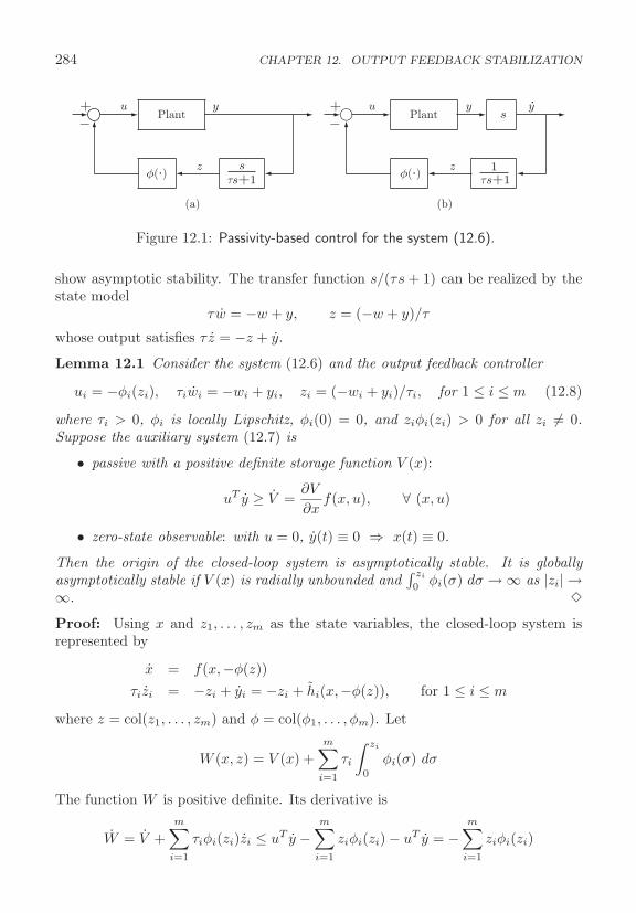
284 CHAPTER 12. OUTPUT FEEDBACK STABILIZATION
Plant
sτs+1
+−
y
z
u
φ(.)τs+1
Plant s
1
+−
z
yu
φ(.)
y.
(a) (b)
Figure 12.1: Passivity-based control for the system (12.6).
show asymptotic stability. The transfer function s/(τs + 1) can be realized by thestate model
τw = −w + y, z = (−w + y)/τ
whose output satisfies τ z = −z + y.
Lemma 12.1 Consider the system (12.6) and the output feedback controller
ui = −φi(zi), τiwi = −wi + yi, zi = (−wi + yi)/τi, for 1 ≤ i ≤ m (12.8)
where τi > 0, φi is locally Lipschitz, φi(0) = 0, and ziφi(zi) > 0 for all zi �= 0.Suppose the auxiliary system (12.7) is
• passive with a positive definite storage function V (x):
uT y ≥ V =∂V
∂xf(x, u), ∀ (x, u)
• zero-state observable: with u = 0, y(t) ≡ 0 ⇒ x(t) ≡ 0.
Then the origin of the closed-loop system is asymptotically stable. It is globallyasymptotically stable if V (x) is radially unbounded and
∫ zi
0φi(σ) dσ → ∞ as |zi| →
∞. �
Proof: Using x and z1, . . . , zm as the state variables, the closed-loop system isrepresented by
x = f(x,−φ(z))τizi = −zi + yi = −zi + hi(x,−φ(z)), for 1 ≤ i ≤ m
where z = col(z1, . . . , zm) and φ = col(φ1, . . . , φm). Let
W (x, z) = V (x) +m∑
i=1
τi
∫ zi
0
φi(σ) dσ
The function W is positive definite. Its derivative is
W = V +m∑
i=1
τiφi(zi)zi ≤ uT y −m∑
i=1
ziφi(zi) − uT y = −m∑
i=1
ziφi(zi)
12.2. PASSIVITY-BASED CONTROL 285
Hence, W is negative semidefinite. Moreover,
W ≡ 0 ⇒ z(t) ≡ 0 ⇒ u(t) ≡ 0 and y(t) ≡ 0
It follows from zero state observability of the auxiliary system (12.7) that x(t) ≡ 0.By the invariance principle we conclude that the origin is asymptotically stable. IfV (x) is radially unbounded and
∫ zi
0φi(σ) dσ → ∞ as |zi| → ∞, the function W
will be radially unbounded and the origin will be globally asymptotically stable. �Similar to our discussion in Section 9.6, if the system (12.7) is not passive we
may be able to turn it into a passive one by feedback passivation. Here, however,passivation will have to be via output feedback.
Example 12.2 Reconsider the regulation problem of an m-link robot from Exam-ple 9.15 when we can measure q but not q. The regulation error e = q − qr satisfiesthe equation
M(q)e + C(q, q)e + De + g(q) = u
with the output y = e. The regulation task is achieved by stabilizing the system at(e = 0, e = 0). With
u = g(q) − Kpe + v
where Kp is a positive definite symmetric matrix, the system is given by
M(q)e + C(q, q)e + De + Kpe = v, y = e
which has an equilibrium point at (e = 0, e = 0) when v = 0. Taking the energy
V = 12 eT M(q)e + 1
2eT Kpe
as the storage function, we have
V = eT Me + 12 eT M e + eT Kpe
= 12 eT (M − 2C)e − eT De − eT Kpe + eT v + eT Kpe ≤ eT v
Hence, the auxiliary system from v to e is passive. It is also zero-state observablebecause, with v = 0,
e(t) ≡ 0 ⇒ e(t) ≡ 0 ⇒ Kpe(t) ≡ 0 ⇒ e(t) ≡ 0
According to Lemma 12.1, the system can be globally stabilized by the controlv = −Kdz where Kd is a positive diagonal matrix and zi is the output of the linearsystem
τiwi = −wi + ei, zi = (−wi + ei)/τi, for 1 ≤ i ≤ m
The overall control u is given by
u = g(q) − Kp(q − qr) − Kdz

286 CHAPTER 12. OUTPUT FEEDBACK STABILIZATION
Comparing this control with the state feedback control
u = g(q) − Kp(q − qr) − Kdq
of Example 9.15 shows that the derivative q of the PD controller is replaced byz, which is obtained by passing ei through the transfer function s/(τis + 1). Weemphasize that zi is not necessarily an approximation of qi because we do not requirethe time constant τi to be small. �
12.3 Observer-Based Control
Consider the systemx = f(x, u), y = h(x) (12.9)
where x ∈ Rn, u ∈ Rm, and y ∈ Rp are the state, control input, and measuredoutput, respectively, f(0, 0) = 0, h(0) = 0, and f(x, u), h(x) are locally Lipschitz.Let u = γ(x) be a locally Lipschitz state feedback controller that stabilizes theorigin of the closed-loop system x = f(x, γ(x)). The observer for (12.9) is taken as
˙x = f(x, u) + H[y − h(x)] (12.10)
The estimation error x = x − x satisfies the equation
˙x = f(x, u) − f(x, u) − H[h(x) − h(x)] def= g(x, x) (12.11)
The equation (12.11) has an equilibrium point at x = 0. We assume that theobserver gain H is designed such that x = 0 is exponentially stable and there is aLyapunov function V1(x) that satisfies the inequalities
c1‖x‖2 ≤ V1(x) ≤ c2‖x‖2,∂V1
∂xg(x, x) ≤ −c3‖x‖2,
∥∥∥∥∂V1
∂x
∥∥∥∥ ≤ c4‖x‖ (12.12)
for all x ∈ D1 and x ∈ D2 for some positive constants c1 to c4, where D1 ⊂ Rn
and D2 ⊂ Rn are domains that contain the origin. We have seen in Sections 11.1and 11.3 observers for which (12.12) is satisfied locally or globally. The closed-loopsystem under output feedback is given by
x = f(x, γ(x − x)), ˙x = g(x, x) (12.13)
The task now is to show that the origin (x = 0, x = 0) is an asymptotically stableequilibrium point of (12.13).
Theorem 12.1 Consider the system (12.13) and suppose that (12.12) is satisfied.
• If the origin of x = f(x, γ(x)) is asymptotically stable, then the origin of(12.13) is asymptotically stable.
12.3. OBSERVER-BASED CONTROL 287
• If the origin of x = f(x, γ(x)) is exponentially stable, then the origin of (12.13)is exponentially stable.
• If (12.12) holds globally and the system x = f(x, γ(x − x)), with input x,is input-to-state stable, then the origin of (12.13) is globally asymptoticallystable.
�
The first two bullets give local results. The third bullet is a global result that re-quires the stronger condition of input-to-state stability. The proof of the theorem isvery similar to the Lyapunov analysis of cascade systems in Section C.1. Althoughthe system (12.13) is not a cascade connection, the origin of ˙x = g(x, x) is expo-nentially stable uniformly in x.
Proof: If the origin of x = f(x, γ(x)) is asymptotically stable, then by (the con-verse Lyapunov) Theorem 3.9, there are positive definite functions V0(x) and W0(x)such that
∂V0
∂xf(x, γ(x)) ≤ −W0(x)
in some neighborhood of x = 0. On a bounded neighborhood of the origin, we canuse the local Lipschitz property of f and γ to obtain∥∥∥∥∂V0
∂x[f(x, γ(x)) − f(x, γ(x − x))]
∥∥∥∥ ≤ L‖x‖
for some positive constant L. Using V (x, x) = bV0(x) +√
V1(x), with b > 0, as aLyapunov function candidate for (12.13), we obtain
V = b∂V0
∂xf(x, γ(x − x)) +
12√
V1
∂V1
∂xg(x, x)
= b∂V0
∂xf(x, γ(x)) + b
∂V0
∂x[f(x, γ(x − x)) − f(x, γ(x))] +
12√
V1
∂V1
∂xg(x, x)
≤ −bW0(x) + bL‖x‖ − c3‖x‖2
2√
V1
SinceV1 ≤ c2‖x‖2 ⇒ −1√
V1
≤ −1√c2 ‖x‖
we haveV ≤ −bW0(x) + bL‖x‖ − c3
2√
c2‖x‖
Choosing b < c3/(2L√
c2) ensure that V is negative definite, which completes theproof of the first bullet.
288 CHAPTER 12. OUTPUT FEEDBACK STABILIZATION
If the origin of x = f(x, γ(x)) is exponentially stable, then by (the converse Lya-punov) Theorem 3.8, there is a Lyapunov function V0(x) that satisfies the inequal-ities
a1‖x‖2 ≤ V0(x) ≤ a2‖x‖2,∂V0
∂xf(x, γ(x)) ≤ −a3‖x‖2,
∥∥∥∥∂V0
∂x
∥∥∥∥ ≤ a4‖x‖
in some neighborhood of the origin, for some positive constants a1 to a4. UsingV (x, x) = bV0(x)+V1(x), with b > 0, as a Lyapunov function candidate for (12.13),we obtain
V = b∂V0
∂xf(x, γ(x)) + b
∂V0
∂x[f(x, γ(x − x)) − f(x, γ(x))] +
∂V1
∂xg(x, x)
≤ −ba3‖x‖2 + ba4L1‖x‖‖x‖ − c3‖x‖2
= −[‖x‖‖x‖]T [
ba3 −ba4L1/2−ba4L1/2 c3
] [‖x‖‖x‖]
where L1 is a Lipschitz constant of f(x, γ(x − x)) with respect to x. Choosingb < 4a3c3/(a4L1)2 ensures that the matrix in the foregoing inequality is positivedefinite, which completes the proof of the second bullet. The proof of the thirdbullet follows from the proof of Lemma 4.6.1 �
If the Lyapunov functions V0(x) for the closed-loop system under state feedbackand V1(x) for the observer are known, the composite Lyapunov functions V =bV0 +
√V1, for the first bullet, and V = bV0 + V1, for the second bullet, can be
used to estimate the region of attraction of the closed-loop system under outputfeedback.
12.4 High-Gain Observers and the Separation Principle
As we did in Section 11.4, we start our study of high-gain observers in feedbackcontrol with a motivating example.
Example 12.3 Consider the two-dimensional system
x1 = x2, x2 = φ(x, u), y = x1 (12.14)
where x = col(x1, x2). Suppose u = γ(x) is a locally Lipschitz state feedbackcontroller that stabilizes the origin of the closed-loop system
x1 = x2, x2 = φ(x, γ(x)) (12.15)
To implement this control with output feedback we use the high-gain observer
˙x1 = x2 + (α1/ε)(y − x1), ˙x2 = φ0(x, u) + (α2/ε2)(y − x1) (12.16)1See [130].
12.4. HIGH-GAIN OBSERVERS AND THE SEPARATION PRINCIPLE 289
where φ0 is a nominal model of φ, and α1, α2, and ε are positive constants withε � 1. We saw in Lemma 11.3 that if
|φ0(z, u) − φ(x, u)| ≤ L ‖x − z‖ + M
over the domain of interest, then for sufficiently small ε, the estimation errorsx1 = x1 − x1 and x2 = x2 − x2 satisfy the inequalities
|x1| ≤ max{
be−at/ε, ε2cM}
, |x2| ≤{
b
εe−at/ε, εcM
}(12.17)
for some positive constants a, b, c. These inequalities show that reducing ε di-minishes the effect of model uncertainty. They show also that, for small ε, theestimation error will be much faster than x. The bound on x2 demonstrates thepeaking phenomenon that was described in Section 11.4; namely, x2 might peakto O(1/ε) values before it decays rapidly towards zero. The peaking phenomenonmight destabilize the closed-loop system. This fact is illustrated by simulating thesystem
x1 = x2, x2 = x32 + u, y = x1
which can be globally stabilized by the state feedback controller
u = −x32 − x1 − x2
The output feedback controller is taken as
u = −x32 − x1 − x2, ˙x1 = x2 + (2/ε)(y − x1), ˙x2 = (1/ε2)(y − x1)
where we took φ0 = 0. Figure 12.2 shows the performance of the closed-loop systemunder state and output feedback. Output feedback is simulated for three differentvalues of ε. The initial conditions are x1(0) = 0.1, x2(0) = x1(0) = x2(0) =0. Peaking is induced by [x1(0) − x1(0)]/ε = 0.1/ε when ε is sufficiently small.Figure 12.2 shows a counter intuitive behavior as ε decreases. Since decreasingε causes the estimation error to decay faster toward zero, one would expect theresponse under output feedback to approach the response under state feedback as εdecreases. Figure 12.2 shows the opposite behavior where the response under outputfeedback deviates from the response under state feedback as ε decreases. This isthe impact of the peaking phenomenon. The same figure shows the control u on amuch shorter time interval to exhibit peaking. This control peaking is transmittedto the plant causing its state to peak. Figure 12.3 shows that as we decrease ε to0.004, the system has a finite escape time shortly after t = 0.07.
Fortunately, we can overcome the peaking phenomenon by saturating the controloutside a compact set of interest in order to create a buffer that protects the plantfrom peaking. Writing the closed-loop system under state feedback as x = Ax andsolving the Lyapunov equation PA + AT P = −I, we have
A =[
0 1−1 −1
]and P =
[1.5 0.50.5 1
]
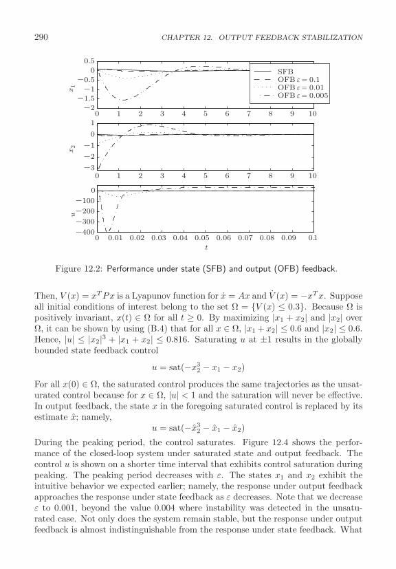
290 CHAPTER 12. OUTPUT FEEDBACK STABILIZATION
0 1 2 3 4 5 6 7 8 9 10−2
−1.5
−1
−0.5
0
0.5
SFBOFB ε = 0.1 OFB ε = 0.01 OFB ε = 0.005
0 1 2 3 4 5 6 7 8 9 10−3
−2
−1
0
1
0 0.01 0.02 0.03 0.04 0.05 0.06 0.07 0.08 0.09 0.1−400
−300
−200
−100
0
t
x1
x2
u
Figure 12.2: Performance under state (SFB) and output (OFB) feedback.
Then, V (x) = xT Px is a Lyapunov function for x = Ax and V (x) = −xT x. Supposeall initial conditions of interest belong to the set Ω = {V (x) ≤ 0.3}. Because Ω ispositively invariant, x(t) ∈ Ω for all t ≥ 0. By maximizing |x1 + x2| and |x2| overΩ, it can be shown by using (B.4) that for all x ∈ Ω, |x1 + x2| ≤ 0.6 and |x2| ≤ 0.6.Hence, |u| ≤ |x2|3 + |x1 + x2| ≤ 0.816. Saturating u at ±1 results in the globallybounded state feedback control
u = sat(−x32 − x1 − x2)
For all x(0) ∈ Ω, the saturated control produces the same trajectories as the unsat-urated control because for x ∈ Ω, |u| < 1 and the saturation will never be effective.In output feedback, the state x in the foregoing saturated control is replaced by itsestimate x; namely,
u = sat(−x32 − x1 − x2)
During the peaking period, the control saturates. Figure 12.4 shows the perfor-mance of the closed-loop system under saturated state and output feedback. Thecontrol u is shown on a shorter time interval that exhibits control saturation duringpeaking. The peaking period decreases with ε. The states x1 and x2 exhibit theintuitive behavior we expected earlier; namely, the response under output feedbackapproaches the response under state feedback as ε decreases. Note that we decreaseε to 0.001, beyond the value 0.004 where instability was detected in the unsatu-rated case. Not only does the system remain stable, but the response under outputfeedback is almost indistinguishable from the response under state feedback. What
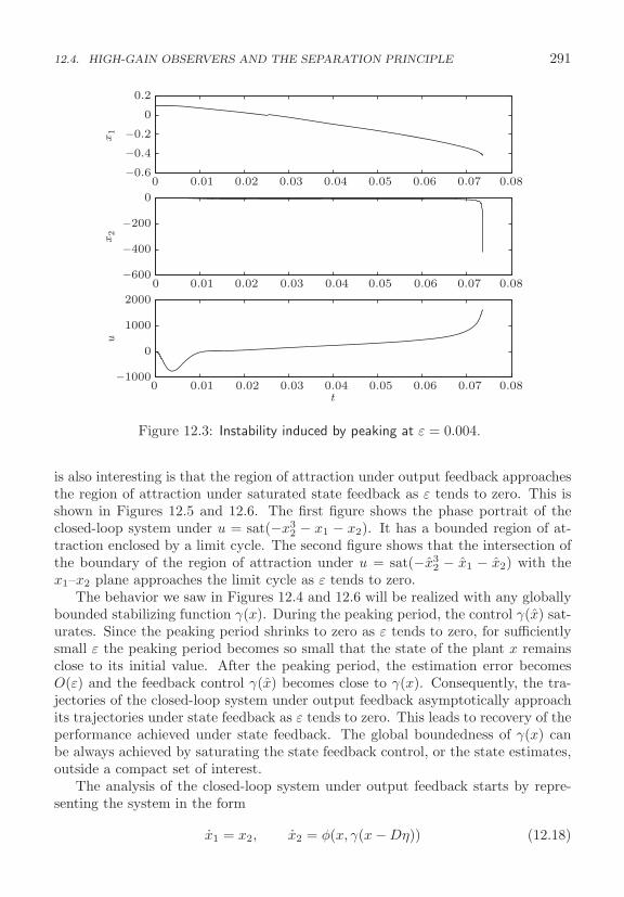
12.4. HIGH-GAIN OBSERVERS AND THE SEPARATION PRINCIPLE 291
0 0.01 0.02 0.03 0.04 0.05 0.06 0.07 0.08−0.6
−0.4
−0.2
0
0.2
0 0.01 0.02 0.03 0.04 0.05 0.06 0.07 0.08−600
−400
−200
0
0 0.01 0.02 0.03 0.04 0.05 0.06 0.07 0.08−1000
0
1000
2000
t
x1
x2
u
Figure 12.3: Instability induced by peaking at ε = 0.004.
is also interesting is that the region of attraction under output feedback approachesthe region of attraction under saturated state feedback as ε tends to zero. This isshown in Figures 12.5 and 12.6. The first figure shows the phase portrait of theclosed-loop system under u = sat(−x3
2 − x1 − x2). It has a bounded region of at-traction enclosed by a limit cycle. The second figure shows that the intersection ofthe boundary of the region of attraction under u = sat(−x3
2 − x1 − x2) with thex1–x2 plane approaches the limit cycle as ε tends to zero.
The behavior we saw in Figures 12.4 and 12.6 will be realized with any globallybounded stabilizing function γ(x). During the peaking period, the control γ(x) sat-urates. Since the peaking period shrinks to zero as ε tends to zero, for sufficientlysmall ε the peaking period becomes so small that the state of the plant x remainsclose to its initial value. After the peaking period, the estimation error becomesO(ε) and the feedback control γ(x) becomes close to γ(x). Consequently, the tra-jectories of the closed-loop system under output feedback asymptotically approachits trajectories under state feedback as ε tends to zero. This leads to recovery of theperformance achieved under state feedback. The global boundedness of γ(x) canbe always achieved by saturating the state feedback control, or the state estimates,outside a compact set of interest.
The analysis of the closed-loop system under output feedback starts by repre-senting the system in the form
x1 = x2, x2 = φ(x, γ(x − Dη)) (12.18)
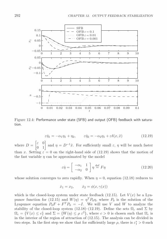
292 CHAPTER 12. OUTPUT FEEDBACK STABILIZATION
0 1 2 3 4 5 6 7 8 9 10−0.05
0
0.05
0.1
0.15
0 1 2 3 4 5 6 7 8 9 10
−0.1
−0.05
0
0.05
0 0.01 0.02 0.03 0.04 0.05 0.06 0.07 0.08 0.09 0.1
−1
−0.5
0
t
SFBOFB ε = 0.1 OFB ε = 0.01 OFB ε = 0.001
x1
x2
u
Figure 12.4: Performance under state (SFB) and output (OFB) feedback with satura-tion.
εη1 = −α1η1 + η2, εη2 = −α2η1 + εδ(x, x) (12.19)
where D =[ε 00 1
]and η = D−1x. For sufficiently small ε, η will be much faster
than x. Setting ε = 0 on the right-hand side of (12.19) shows that the motion ofthe fast variable η can be approximated by the model
εη =[ −α1 1
−α2 0
]η
def= Fη (12.20)
whose solution converges to zero rapidly. When η = 0, equation (12.18) reduces to
x1 = x2, x2 = φ(x, γ(x))
which is the closed-loop system under state feedback (12.15). Let V (x) be a Lya-punov function for (12.15) and W (η) = ηT P0η, where P0 is the solution of theLyapunov equation P0F + FT P0 = −I. We will use V and W to analyze thestability of the closed-loop system (12.18)–(12.19). Define the sets Ωc and Σ byΩc = {V (x) ≤ c} and Σ = {W (η) ≤ ρ ε2}, where c > 0 is chosen such that Ωc isin the interior of the region of attraction of (12.15). The analysis can be divided intwo steps. In the first step we show that for sufficiently large ρ, there is ε∗1 > 0 such
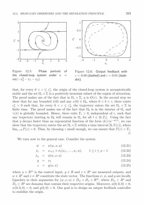
12.4. HIGH-GAIN OBSERVERS AND THE SEPARATION PRINCIPLE 293
−3 −2 −1 0 1 2 3−2
−1
0
1
2
x1
x2
Figure 12.5: Phase portrait ofthe closed-loop system under u =sat(−x3
2 − x1 − x2).
−2 −1 0 1 2
−1
−0.5
0
0.5
1
x1
x2
Figure 12.6: Output feedback withε = 0.08 (dashed) and ε = 0.01 (dash-dot).
that, for every 0 < ε ≤ ε∗1, the origin of the closed-loop system is asymptoticallystable and the set Ωc ×Σ is a positively invariant subset of the region of attraction.The proof makes use of the fact that in Ωc × Σ, η is O(ε). In the second step weshow that for any bounded x(0) and any x(0) ∈ Ωb, where 0 < b < c, there existsε∗2 > 0 such that, for every 0 < ε ≤ ε∗2, the trajectory enters the set Ωc × Σ infinite time. The proof makes use of the fact that Ωb is in the interior of Ωc andγ(x) is globally bounded. Hence, there exits T1 > 0, independent of ε, such thatany trajectory starting in Ωb will remain in Ωc for all t ∈ [0, T1]. Using the factthat η decays faster than an exponential function of the form (k/ε)e−at/ε, we canshow that the trajectory enters the set Ωc×Σ within a time interval [0, T (ε)], wherelimε→0 T (ε) = 0. Thus, by choosing ε small enough, we can ensure that T (ε) < T1.
�We turn now to the general case. Consider the system
w = ψ(w, x, u) (12.21)xi = xi+1 + ψi(x1, . . . , xi, u), 1 ≤ i ≤ ρ − 1 (12.22)xρ = φ(w, x, u) (12.23)y = x1 (12.24)z = q(w, x) (12.25)
where u ∈ Rm is the control input, y ∈ R and z ∈ Rs are measured outputs, andw ∈ R� and x ∈ Rρ constitute the state vector. The functions ψ, φ, and q are locallyLipschitz in their arguments for (w, x, u) ∈ Dw × Dx × Rm, where Dw ⊂ Rs andDx ⊂ Rρ are domains that contain their respective origins. Moreover, φ(0, 0, 0) = 0,ψ(0, 0, 0) = 0, and q(0, 0) = 0. Our goal is to design an output feedback controllerto stabilize the origin.
294 CHAPTER 12. OUTPUT FEEDBACK STABILIZATION
When ψ1 = · · · = ψρ = 0, equations (12.22)–(12.23) represent a chain of ρintegrators. The two main sources for the model (12.21)–(12.25) in this case arethe normal form of Section 8.1 and models of mechanical and electromechanicalsystems where displacement variables are measured while their derivatives (veloc-ities, accelerations, etc.) are not measured. When ψ1 to ψρ−1 are independentof u, equations (12.22)–(12.23) are in the strict feedback form (9.17). If y is theonly measured variable, we can drop equation (12.25). However, in many problems,we can measure some state variables in addition to y. For example, the magneticlevitation system of Section A.8 is modeled by
x1 = x2
x2 = −bx2 + 1 − 4cx23
(1 + x1)2
x3 =1
T (x1)
[−x3 + u +
βx2x3
(1 + x1)2
]where the normalized variables x1, x2, and x3 are the ball position, its velocity, andthe electromagnet current, respectively. Typically, we measure the ball position x1
and the current x3. The model fits the form (12.21)–(12.25) with (x1, x2) as thex component and x3 as the w component. The measured outputs are y = x1 andz = x3.
We use a two-step approach to design the output feedback controller. First, apartial state feedback controller that uses measurements of x and z is designed toasymptotically stabilize the origin. Then, a high-gain observer is used to estimatex from y. The state feedback controller is allowed to be a dynamical system of theform
ϑ = Γ(ϑ, x, z), u = γ(ϑ, x, z) (12.26)
where γ and Γ are locally Lipschitz functions in their arguments over the domainof interest and globally bounded functions of x. Moreover, γ(0, 0, 0) = 0 andΓ(0, 0, 0) = 0. A static state feedback controller u = γ(x, z) is a special case ofthe foregoing equation by dropping the ϑ-equation. The more general form (12.26)allows us to include, among other things, integral control as we shall see in Chap-ter 13. If the functions γ and Γ are not globally bounded in x we can saturatethem or their x entries outside a compact set of x. The saturation levels can bedetermined by analytically calculated bounds, as it was done in Example 12.3, orby extensive simulations that cover several initial conditions in the compact set ofinterest.
For convenience, we write the closed-loop system under state feedback as
X = f(X ) (12.27)
where X = col(w, x, ϑ). The output feedback controller is taken as
ϑ = Γ(ϑ, x, z), u = γ(ϑ, x, z) (12.28)

12.4. HIGH-GAIN OBSERVERS AND THE SEPARATION PRINCIPLE 295
where x is generated by the high-gain observer
˙xi = xi+1 + ψi(x1, . . . , xi, u) +αi
εi(y − x1), for 1 ≤ i ≤ ρ − 1 (12.29)
˙xρ = φ0(x, z, u) +αρ
ερ(y − x1) (12.30)
where ε is a sufficiently small positive constant, and α1 to αρ are chosen such thatthe roots of
sρ + α1sρ−1 + · · · + αρ−1s + αρ = 0 (12.31)
have negative real parts. The function φ0(x, z, u) implements φ0(x, z, u), which is anominal model of φ(w, x, u) that is required to be locally Lipschitz in its argumentsover the domain of interest and globally bounded in x. Moreover, φ0(0, 0, 0) = 0.The following theorem states the properties of the closed-loop system under theoutput feedback controller.2
Theorem 12.2 Consider the closed-loop system of the plant (12.21)–(12.25) andthe output feedback controller (12.28)–(12.30). Suppose the origin of (12.27) isasymptotically stable and R is its region of attraction. Let S be any compact setin the interior of R and Q be any compact subset of Rρ. Then, given any μ > 0there exist ε∗ > 0 and T ∗ > 0, dependent on μ, such that for every 0 < ε ≤ ε∗, thesolutions (X (t), x(t)) of the closed-loop system, starting in S × Q, are bounded forall t ≥ 0 and satisfy
‖X (t)‖ ≤ μ and ‖x(t)‖ ≤ μ, ∀ t ≥ T ∗ (12.32)
‖X (t) −Xr(t)‖ ≤ μ, ∀ t ≥ 0 (12.33)
where Xr is the solution of (12.27), starting at X (0). Moreover, if the origin of(12.27) is exponentially stable, then the origin of the closed-loop system is exponen-tially stable and S ×Q is a subset of its region of attraction. �
The theorem shows a number of properties of the output feedback controller whenε is sufficiently small. First, (12.32) shows that the trajectories can be brought toan arbitrarily small neighborhood of the origin by choosing ε small enough. Second,(12.33) shows that the solution X (t) under output feedback approaches the solutionXr(t) under state feedback as ε tends to zero. Third, the output feedback controllerrecovers the region of attraction of the state feedback controller in the sense thatthe foregoing two properties hold for any compact set in the interior of the regionof attraction. Finally, it recovers exponential stability when the origin under statefeedback is exponentially stable.3 As a corollary of the theorem, it is clear that if
2The theorem is proved in [74, Theorem 14.6] for the case when ψ1 = · · · = ψρ−1 = 0. Thepresence of ψi’s does not alter the proof in view of the fact, shown in Section 11.4, that the scaledestimation error η satisfies equation (11.36) where δ satisfies (11.37). The steps of the proof areoutlined in Example 12.3.
3For convenience, recovery of asymptotic stability is shown only for the exponentially stablecase. See [9] for the more general case when the origin is asymptotically, but not exponentially,stable.
296 CHAPTER 12. OUTPUT FEEDBACK STABILIZATION
the state feedback controller achieves global or semiglobal stabilization with localexponential stability, then for sufficiently small ε, the output feedback controllerachieves semiglobal stabilization with local exponential stability.
The trajectory recovery property (12.33) has a significant practical implicationbecause it allows the designer to design the state feedback controller to meet tran-sient response specifications, constraints on the state variables, and/or constraintson the control inputs. Then, by saturating the state estimate x and/or the controlu outside compact sets of interest to make the functions γ(ϑ, x, z), Γ(ϑ, x, z), andφ0(x, z, u) globally bounded function in x, he/she can proceed to tune the parame-ter ε by decreasing it monotonically to bring the trajectories under output feedbackclose enough to the ones under state feedback. This establishes a separation prin-ciple where the state feedback design is separated from the observer design.
12.5 Robust Stabilization of Minimum Phase Systems
In this section we consider a single-input–single-output nonlinear system that hasrelative degree ρ and can be transformed into the normal form of Section 8.1. Weassume that the system is minimum phase. Our goal is to design a feedback con-troller to stabilize the origin in the presence of matched model uncertainty andtime-varying disturbance. In Section 12.5.1, the system has relative degree one.The design of a robust stabilizing controller in this case follows in a straightforwardway from the state feedback stabilization techniques of Chapter 10. We designa sliding mode controller. In Section 12.5.2 we consider a system of relative de-gree higher than one and show how high-gain observers can be used to reduce thestabilization problem to that of a relative-degree-one system.
12.5.1 Relative Degree One
When ρ = 1, the normal form is given by
η = f0(η, y), y = a(η, y) + b(η, y)u + δ(t, η, y, u) (12.34)
where η ∈ Rn−1, u ∈ R, y ∈ R, the functions f0, a and b are locally Lipschitz,f0(0, 0) = 0, and a(0, 0) = 0. Equation (12.34) includes a matched time-varyingdisturbance δ, which is assumed to be piecewise continuous in t and locally Lipschitzin (η, y, u). Let D ⊂ Rn be a domain that contains the origin and assume that forall (η, y) ∈ D, b(η, y) ≥ b0 > 0. Equation (12.34) is in the regular form (10.4)with ξ = y. Because the system is minimum phase, the origin of η = f0(η, 0) isasymptotically stable. Therefore, we can take the sliding surface as y = 0. Weassume that there is a (continuously differentiable) Lyapunov function V (η) thatsatisfies the inequalities
α1(‖η‖) ≤ V (η) ≤ α2(‖η‖) (12.35)
12.5. ROBUST STABILIZATION OF MINIMUM PHASE SYSTEMS 297
∂V
∂ηf0(η, y) ≤ −α3(‖η‖), ∀ ‖η‖ ≥ α4(|y|) (12.36)
for all (η, y) ∈ D, where α1 to α4 are class K functions. By Theorem 4.7, inequality(12.36) implies regional input-to-state stability of the system η = fa(η, y) with inputy. Similar to (10.7), we take the control as
u = ψ(y) + v
where ψ could be zero or could be chosen to cancel part of the known term on theright-hand side of y, which depends only on y. We assume that we know a locallyLipschitz function �(y) ≥ 0 and a constant κ0 ∈ [0, 1) such that the inequality∣∣∣∣a(η, y) + b(η, y)ψ(y) + δ(t, η, y, ψ(y) + v)
b(η, y)
∣∣∣∣ ≤ �(y) + κ0|v| (12.37)
holds for all t ≥ 0, (η, y) ∈ D, and u ∈ R. Similar to (10.12), take v as
v = −β(y) sat(
y
μ
)where β(y) is a locally Lipschitz function that satisfies
β(y) ≥ �(y)1 − κ0
+ β0 (12.38)
for some β0 > 0. The overall control
u = ψ(y) − β(y) sat(
y
μ
)(12.39)
is similar to the state feedback case except that we take s = y and restrict β and ψto be functions of y rather than the whole state vector. The following two theoremsare corollaries of Theorems 10.1 and 10.2.
Theorem 12.3 Consider the system (12.34). Suppose there exist V (η), �(y), andκ0, which satisfy (12.35), (12.36), and (12.37). Let u be given by (12.39) where βsatisfies (12.38). Define the class K function α by α(r) = α2(α4(r)) and suppose μ,c > μ, and c0 ≥ α(c) are chosen such that the set
Ω = {V (η) ≤ c0} × {|y| ≤ c}, with c0 ≥ α(c) (12.40)
is compact and contained in D. Then, Ω is positively invariant and for any initialstate in Ω, the state is bounded for all t ≥ 0 and reaches the positively invariant set
Ωμ = {V (η) ≤ α(μ)} × {|y| ≤ μ} (12.41)
in finite time. If the assumptions hold globally and V (η) is radially unbounded, theforegoing conclusion will hold for any initial state. �
298 CHAPTER 12. OUTPUT FEEDBACK STABILIZATION
Theorem 12.4 Suppose all the assumptions of Theorem 12.3 are satisfied with�(0) = 0 and the origin of η = f0(η, 0) is exponentially stable. Then, there existsμ∗ > 0 such that for all 0 < μ < μ∗, the origin of the closed-loop system is ex-ponentially stable and Ω is a subset of its region of attraction. If the assumptionshold globally and V (η) is radially unbounded, the origin will be globally uniformlyasymptotically stable. �
12.5.2 Relative Degree Higher Than One
The normal form of a system having relative degree ρ > 1 is given by
η = f0(η, ξ) (12.42)ξi = ξi+1, for 1 ≤ i ≤ ρ − 1 (12.43)ξρ = a(η, ξ) + b(η, ξ)u + δ(t, η, ξ, u) (12.44)y = ξ1 (12.45)
where η ∈ Rn−ρ, ξ = col(ξ1, ξ2, . . . , ξρ), u ∈ R, y ∈ R, and the functions f0, a andb are locally Lipschitz. The matched disturbance δ is piecewise continuous in t andlocally Lipschitz in (η, ξ, u). Let D ⊂ Rn be a domain that contains the origin andassume that for all (η, ξ) ∈ D, b(η, ξ) ≥ b0 > 0. Because the system is minimumphase, the origin of η = f0(η, 0) is asymptotically stable.
From the properties of high-gain observers, presented in Section 11.4, and theseparation principle of Section 12.4, we expect that if we can design a partial statefeedback controller, in terms of ξ, which stabilizes or practically stabilizes the origin,we will be able to recover its performance by using a high-gain observer to estimateξ. Based on this expectation we will proceed to design a controller that uses feedbackfrom ξ.4
With measurement of ξ we can convert the relative-degree-ρ system into arelative-degree-one system with respect to the output
s = k1ξ1 + k2ξ2 + · · · + kρ−1ξρ−1 + ξρ (12.46)
The normal form of this system is given by
z = f0(z, s), s = a(z, s) + b(z, s)u + δ(t, z, s, u) (12.47)
where
z =
⎡⎢⎢⎢⎢⎢⎣
ηξ1
...ξρ−2
ξρ−1
⎤⎥⎥⎥⎥⎥⎦ , f0(z, s) =
⎡⎢⎢⎢⎢⎢⎣
f0(η, ξ)ξ2
...ξρ−1
ξρ
⎤⎥⎥⎥⎥⎥⎦ , a(z, s) =
ρ−1∑i=1
kiξi+1 + a(η, ξ)
4Alternatively, robust stabilization can be achieved using sliding mode observers [85, 124].
12.5. ROBUST STABILIZATION OF MINIMUM PHASE SYSTEMS 299
b(z, s) = b(η, ξ), δ(t, z, s, u) = δ(t, η, ξ, u)
with ξρ = s −∑ρ−1i=1 kiξi. The functions f0, a, b, and δ inherit the properties of
f0, a, b, and δ, respectively. In particular, b(z, s) ≥ b0 > 0 for all (η, ξ) ∈ D. Thezero dynamic of (12.47) is z = f0(z, 0). This system can be written as the cascadeconnection
η = f0(η, ξ)
∣∣∣∣∣∣ξρ=−∑ρ−1
i=1 kiξi
, ζ = Fζ (12.48)
where
ζ =
⎡⎢⎢⎢⎣
ξ1
ξ2
...ξρ−1
⎤⎥⎥⎥⎦ , F =
⎡⎢⎢⎢⎢⎢⎣
0 1 0 · · · 00 0 1 · · · 0...
...0 · · · 0 1
−k1 −k2 · · · −kρ−2 −kρ−1
⎤⎥⎥⎥⎥⎥⎦
Because the origin η = 0 of η = f0(η, 0) is asymptotically stable by the mini-mum phase assumption, the origin z = 0 of the cascade connection (12.48) will beasymptotically stable if the matrix F is Hurwitz. Therefore, k1 to kρ−1 in (12.46)are chosen such that the polynomial
λρ−1 + kρ−1λρ−2 + · · · + k2λ + k1 (12.49)
is Hurwitz; that is, all its roots have negative real parts. Consequently, k1 to kρ−1
are positive constants. As in Section C.1, asymptotic stability of the origin of thecascade connection (12.48) can be shown by the Lyapunov function V1(z) = cV0(η)+√
ζT Pζ, where V0 is a Lyapunov function of η = f0(η, 0), which is guaranteed toexist by (the converse Lyapunov) Theorem 3.9, P is the positive definite solutionof the Lyapunov equation PF + FT P = −I, and c is a sufficiently small positiveconstant. The function V1(z) is not continuously differentiable in the neighborhoodof the origin because it is not continuously differentiable on the manifold ζ = 0.However, once we establish asymptotic stability of the origin of (12.48), Theorem 3.9ensures the existence of a smooth Lyapunov function. Using the local Lipschitzproperty of f0(z, s) with respect to s, it is reasonable to assume that there is a(continuously differentiable) Lyapunov function V (z) that satisfies the inequalities
α1(‖z‖) ≤ V (z) ≤ α2(‖z‖) (12.50)
∂V
∂ηf0(z, s) ≤ −α3(‖z‖), ∀ ‖z‖ ≥ α4(|s|) (12.51)
for all (η, ξ) ∈ D, where α1 to α4 are class K functions. Another property of thecascade connection (12.48) is that its origin z = 0 will be exponentially stable if theorigin η = 0 of η = f0(η, 0) is exponentially stable. This is shown in Section C.1.We note that if ρ = n the zero dynamics of (12.47) will be ζ = Fζ.
300 CHAPTER 12. OUTPUT FEEDBACK STABILIZATION
Thus, we have converted a relative-degree-ρ system into a relative-degree-onesystem that satisfies the assumptions of Section 12.5.1. We proceed to design asliding mode controller as in Section 12.5.1, with the exception that the functionsψ, �, and β will be allowed to depend on the whole vector ξ and not only the outputs since we are working under the assumption that ξ is measured. Let
u = ψ(ξ) + v
for some locally Lipschitz function ψ, with ψ(0) = 0, and suppose we know a locallyLipschitz function �(ξ) ≥ 0 and a constant κ0 ∈ [0, 1) such that the inequality∣∣∣∣∣∑ρ−1
i=1 kiξi+1 + a(η, ξ) + b(η, ξ)ψ(ξ) + δ(t, η, ξ, ψ(ξ) + v)b(η, ξ)
∣∣∣∣∣ ≤ �(ξ) + κ0|v| (12.52)
holds for all t ≥ 0, (η, ξ) ∈ D, and u ∈ R. We note that the left-hand side of (12.52)is the same as ∣∣∣∣ a(z, s) + b(z, s)ψ(ξ) + δ(t, z, s, ψ(ξ) + v)
b(z, s)
∣∣∣∣Similar to (10.12), take v as
v = −β(ξ) sat(
s
μ
)
where β(ξ) is a locally Lipschitz function that satisfies
β(ξ) ≥ �(ξ)1 − κ0
+ β0 (12.53)
for some β0 > 0. The overall control
u = ψ(ξ) − β(ξ) sat(
s
μ
)def= γ(ξ) (12.54)
is similar to the state feedback case except that we restrict β and ψ to be functionsof ξ rather than the whole state vector. Define the class K function α by α(r) =α2(α4(r)) and suppose μ, c > μ, and c0 ≥ α(c) are chosen such that the set
Ω = {V (z) ≤ c0} × {|s| ≤ c}, with c0 ≥ α(c) (12.55)
is compact and contained in D. By Theorem 10.1 we conclude that Ω is positivelyinvariant and for all initial states in Ω, the trajectories enter the positively invariantset
Ωμ = {V (z) ≤ α(μ)} × {|s| ≤ μ} (12.56)
in finite time. If �(0) = 0 and the origin of η = f0(η, 0) is exponentially stable,then Theorem 10.2 shows that there exists μ∗ > 0 such that for all 0 < μ < μ∗,

12.5. ROBUST STABILIZATION OF MINIMUM PHASE SYSTEMS 301
the origin of the closed-loop system is exponentially stable and Ω is a subset of itsregion of attraction.
To implement the partial state feedback controller (12.54) using a high-gainobserver, we start by saturating the control outside the compact set Ω to make it aglobally bounded function of ξ. This is needed to overcome the peaking phenomenonof high-gain observers.5 There are different ways to saturate the control. We cansaturate each component of ξ in the functions ψ and β. Let
Mi = maxΩ
{|ξi|}, 1 ≤ i ≤ ρ
and take ψs and βs as the functions ψ and β with ξi replaced Mi sat(ξi/Mi).Alternatively, let
Mψ = maxΩ
{|ψ(ξ)|}, Mβ = maxΩ
{|β(ξ)|}
and take ψs(ξ) = Mψ sat(ψ(ξ)/Mψ) and βs(ξ) = Mβ sat(β(ξ)/Mβ). In either case,the control is taken as
u = ψs(ξ) − βs(ξ) sat(
s
μ
)We may also saturate the control signal itself. Let
Mu = maxΩ
{|ψ(ξ) − β(x) sat(s/μ)|}
and take the control as
u = Mu sat(
ψ(ξ) − β(ξ) sat(s/μ)Mu
)
Irrespective of how we saturate the control (12.54), the saturation will not be activefor all initial states in Ω because the saturated control coincides with the originalcontrol (12.54) over Ω. We use the high-gain observer
˙ξi = ξi+1 +
αi
εi(y − ξ1), 1 ≤ i ≤ ρ − 1 (12.57)
˙ξρ = a0(ξ) + b0(ξ)u +
αρ
ερ(y − ξ1) (12.58)
to estimate ξ by ξ, where ε is a sufficiently small positive constant, α1 to αρ arechosen such that the polynomial
sρ + α1sρ−1 + · · · + αρ−1s + αρ (12.59)
is Hurwitz, and a0(ξ) and b0(ξ) are locally Lipschitz, globally bounded functions ofξ, which serve as nominal models of a(η, ξ) and b(η, ξ), respectively. The functions
5See Sections 11.4 and 12.4.
302 CHAPTER 12. OUTPUT FEEDBACK STABILIZATION
a0 and b0 are not allowed to depend on η because it is not estimated by the observer(12.57)–(12.58). The choice a0 = b0 = 0 results in a linear observer. This choice istypically used when no good models of a and b are available, or when it is desiredto use a linear observer. The output feedback controller is taken as
u = γs(ξ) (12.60)
where γs(ξ) is given by
ψs(ξ) − βs(ξ) sat(s/μ) or Mu sat
(ψ(ξ) − β(ξ) sat(s/μ)
Mu
)
and
s =ρ−1∑i=1
kiξi + ξρ
The properties of the output feedback controller are stated in the followingtheorems, whose proofs are given in Appendix D.
Theorem 12.5 Consider the system (12.42)–(12.45) and let k1 to kρ−1 be chosensuch that the polynomial (12.49) is Hurwitz. Suppose there exist V (z), �(ξ), and κ0,which satisfy (12.50), (12.51), and (12.52), and β is chosen to satisfy (12.53). LetΩ and Ωμ be defined by (12.55) and (12.56), respectively. Consider the high-gainobserver (12.57)–(12.58), where α1 to αρ are chosen such that the polynomial (12.59)is Hurwitz, and the output feedback controller (12.60). Let Ω0 be a compact set inthe interior of Ω and X be a compact subset of Rρ. Suppose the initial states satisfy(η(0), ξ(0)) ∈ Ω0 and ξ(0) ∈ X. Then, there exists ε∗, dependent on μ, such that forall ε ∈ (0, ε∗) the states (η(t), ξ(t), ξ(t)) of the closed-loop system are bounded forall t ≥ 0 and there is a finite time T , dependent on μ, such that (η(t), ξ(t)) ∈ Ωμ
for all t ≥ T . Moreover, if (ηr(t), ξr(t)) is the state of the closed-loop systemunder the state feedback controller (12.54) with initial conditions ηr(0) = η(0) andξr(0) = ξ(0), then given any λ > 0, there exists ε∗∗ > 0, dependent on μ and λ,such that for all ε ∈ (0, ε∗∗),
‖η(t) − ηr(t)‖ ≤ λ and ‖ξ(t) − ξr(t)‖ ≤ λ, ∀ t ∈ [0, T ] (12.61)
�
Theorem 12.6 Suppose all the assumptions of Theorems 12.5 are satisfied with�(0) = 0 and the origin of η = f0(η, 0) is exponentially stable. Then, there existsμ∗ > 0 and for each μ ∈ (0, μ∗) there exists ε∗ > 0, dependent on μ, such that for allε ∈ (0, ε∗), the origin of the closed-loop system under the output feedback controller(12.60) is exponentially stable and Ω0 ×X is a subset of its region of attraction. �
Theorems 12.5 and 12.6 show that the output feedback controller (12.60) recoversthe stabilization or practical stabilization properties of the state feedback controller(12.54) for sufficiently small ε. It also recovers its transient behavior, as shown by(12.61).

12.6. EXERCISES 303
Example 12.4 In Example 10.1, we designed the state feedback controller
u = −2(|x1| + |x2| + 1) sat(
s
μ
)
where x1 = θ − π, x2 = θ, s = x1 + x2, and μ < 0.308 to stabilize the pendulum
θ + sin θ + bθ = cu
at (θ = π, θ = 0) under the assumption that 0 ≤ b ≤ 0.2 and 0.5 ≤ c ≤ 2. Let ustake μ = 0.1. The controller achieves global stabilization. Suppose now that weonly measure θ. In preparation for using a high-gain observer, we will saturate thestate feedback control outside a compact set. With V1(x) = 1
2x21, the set Ω is given
by Ω = {|x1| ≤ c/θ1} × {|s| ≤ c}, where c > 0 and 0 < θ1 < 1. Suppose that withc = 2π and θ = 0.8, Ω includes all the initial states of interest. Over Ω, we have|x1| ≤ 2.5π and |x2| ≤ 4.5π. Therefore, the output feedback controller is taken as
u = −2(
2.5π sat( |x1|
2.5π
)+ 4.5π sat
( |x2|4.5π
)+ 1)
sat(
s
μ
)where s = x1 + x2 and x = col(x1, x2) is determined by the high-gain observer
˙x1 = x2 +2ε(x1 − x1), ˙x2 = φ0(x, u) +
1ε2
(x1 − x1)
with sufficiently small ε. We will consider two choices of φ0. The first choice φ0 = 0yields a linear observer. The second choice φ0(x) = − sin(x1 + π) − 0.1x2 + 1.25uduplicates the right-hand side of the state equation with 0.1 and 1.25 as nominalvalues of b and c, respectively. In Figure 12.7, we compare the performance of thestate and output feedback controllers for ε = 0.05 and ε = 0.01. The pendulumparameters are b = 0.01 and c = 0.5, and the initial conditions are θ(0) = θ(0) =x1(0) = x2(0) = 0. Peaking is induced because x1(0) = −π �= x1(0). Irrespectiveof the choice of φ0, the simulation results show that the response under outputfeedback approaches the one under state feedback as ε decreases. For ε = 0.01, theinclusion of φ0 in the observer has little effect on the response. However, for thelarger value ε = 0.05, there is an advantage for including φ0 in the observer.6
12.6 Exercises
12.1 For each of the following systems, design a globally stabilizing output feed-back controller.
(1) x1 = x2, x2 = −x31 + tanh(u), y = x2
6Other simulation results, as in [74, Example 14.19], show that the advantage of including φ0
may not be realized if it is not a good model of the state equation.

304 CHAPTER 12. OUTPUT FEEDBACK STABILIZATION
0 1 2 30
0.5
1
1.5
2
2.5
3
3.5
θ
0 1 2 30
1
2
3
4
ω
0 1 2 30
0.5
1
1.5
2
2.5
3
3.5
θ
Time
0 1 2 30
1
2
3
4
Time
ω
(c)
(a) (b)
(d)
SF
OF ε = 0.05
OF ε = 0.01
Figure 12.7: Comparison of state feedback (SF) and output feedback (OF) for Exam-ple 12.4. Figures (a) and (b) show θ and ω = θ for a linear high-gain observer withφ0 = 0. Figures (c) and (d) show θ and ω for a nonlinear high-gain observer withφ0 = − sin(x1 + π) − 0.1x2 + 1.25u.
(2) x1 = x2, x2 = −x31 + tanh(u), y = x1
(3) x1 = β1(x1) + x2, x2 = β2(x1) + β3(x1)x2 + u, y = x1
(4) x1 = sin x1 + x2, x2 = u, y = x1
12.2 For each of the following systems, design a stabilizing output feedback con-troller such that the set {|x1| ≤ 1, |x2| ≤ 1} is included in the region of attraction.
(1) x1 = x1 + x2/(1 + x21), x2 = −x2 + u, y = x1
(2) x1 = ax21 + x2, x2 = u, y = x1, a is unknown with |a| ≤ 1
(3) x1 = x2, x2 = −x2|x2| + u, y = x1

12.6. EXERCISES 305
(4) x1 = x31 + x2, x2 = x1x2 + u, x3 = x1x2 − x3, y = x1
12.3 Consider the inverted pendulum on a cart (A.41)–(A.44), where it is requiredto stabilize the pendulum at (θ, y) = (0, 0) and the measured outputs are θ and y.
(a) Using linearization with the (A.45) data, design a stabilizing output feedbackcontroller.
(b) Using simulation, find the range of x1(0), when all other initial conditions arezero, for which the pendulum is stabilized.
12.4 Consider the inverted pendulum (A.47) with the state feedback controller ofExercise 9.5(a). Suppose you can only measure θ.
(a) With a = 1, design an observer with linear error dynamics and use it to im-plement the controller. Use simulation to find the range of x1(0), when allother initial conditions are zero, for which the pendulum is stabilized and|x1(t)| ≤ π/2 for all t. Compare the performance of the state and outputfeedback controllers.
(b) Repeat (a) using a high-gain observer with ε = 0.01 and saturated control.
(c) Compare the performance of the two observers when a = 1 in the controllerbut it is perturbed in the pendulum with a ∈ [0.5, 1.5].
12.5 Repeat Exercise 12.4 for the the state feedback controller of Exercise 9.5(b).
12.6 Repeat Exercise 12.4 for the the state feedback controller of Exercise 10.10.
12.7 Consider the state feedback controller of Exercise 9.8(b) for the magneticlevitation system.
(a) Implement the controller, using a high-gain observer and saturated control,when the measured output is y = col(x1, x3).
(b) Repeat (a) when y = x1. Hint: Transform the system into the form (11.26)–(11.28).
(c) Use simulation to compare the performance of the state and output feedbackcontrollers.
12.8 Repeat Exercise 12.7 for the the state feedback controller of Exercises 9.8(d).
12.9 Repeat Exercise 12.7 for the the state feedback controller of Exercises 9.8(e).
12.10 Repeat Exercise 12.7 for the the state feedback controller of Exercises 10.7.Take into consideration the uncertainty of b and c.

306 CHAPTER 12. OUTPUT FEEDBACK STABILIZATION
12.11 Consider the electrostatic microactuator (A.33).
(a) Assuming you can only measure x1 and x3, design an observer with linearerror dynamics to implement the state feedback controller of Exercise 9.9(b).Use simulation to compare the performance of the state and output feedbackcontrollers when x(0) = col(0.1, 0,
√0.3) and x(0) = 0.
(b) If you can only measure x1, repeat (a) using a high-gain observer.
12.12 Repeat Exercise 12.11 for the controller of Exercise 9.9(d).
12.13 Repeat Exercise 12.11 for the controller of Exercise 9.9(e).
12.14 Repeat Exercise 12.11 for the controller of Exercise 9.9(f).
12.15 Consider the electrostatic microactuator (A.33) where you can only measurex3. Design an output feedback controller to stabilize the plate at x1 = r. Assumethat ζ ∈ [0.1, 0.5], T ∈ [0.1, 0.5], and r ∈ [0.1, 0.9]. Simulate the closed-loop systemwith r = 0.5, ζ = 0.1, T = 0.2, and x(0) = col(0.1, 0,
√0.3).
12.16 Consider the two-link manipulator defined by (A.36) and (A.37) with the(A.38) data. Assume that the measured output is y = col(q1, q2). It is desired toregulate the manipulator to qr = (π/2, π/2) under the control constraints |u1| ≤6000 and |u2| ≤ 5000. Design a passivity-based controller that meets the controlconstraints. Hint: See Example 12.2 and note that you will need to replace Kpeand Kdz by nonlinear functions.
12.17 Consider the TORA system of (A.49)–(A.52) where the measured outputis y = x1 = θ. Design a globally stabilizing output feedback controller. Hint: SeeExercises 5.10 and 9.13.
12.18 Consider the sliding mode controller of the TORA system in Exercise 10.13.Design a high-gain observer to implement this controller with constant β when themeasured output is y = col(x1, x3). Compare the performance of the state andoutput feedback controllers using the (A.53) data and the controller parameters ofExercise 10.14(a).
12.19 Repeat Problems (1) to (5) of Exercise 10.1 with the goal of achievingsemiglobal stabilization when you only measure x1.

Chapter 13
Tracking and Regulation
In this chapter we study tracking and regulation problems for single-input–single-output systems representable in the normal form:
η = f0(η, ξ) (13.1)ξi = ξi+1, for 1 ≤ i ≤ ρ − 1 (13.2)ξρ = a(η, ξ) + b(η, ξ)u (13.3)y = ξ1 (13.4)
where η ∈ Dη ⊂ Rn−ρ, ξ = col(ξ1, . . . , ξρ) ∈ Dξ ⊂ Rn, for some domains Dη and Dξ.The functions f0, a, and b are locally Lipschitz and b �= 0 over Dη ×Dξ. When therelative degree ρ = n, the system has no zero dynamics. In this case, the η variableand its equation are dropped, but the rest of the development remains the same.The goal of the tracking problem is to design a feedback controller such that theoutput y asymptotically tracks a reference signal r; that is, limt→∞[y(t)−r(t)] = 0,while ensuring boundedness of all state variables. The regulation problem is aspecial case of the tracking problem when r is constant. We assume that the system(13.1)–(13.4) and the reference signal satisfy the following assumptions.
Assumption 13.1
b(η, ξ) ≥ b0 > 0, ∀ η ∈ Dη, ξ ∈ Dξ
Assumption 13.2 The system η = f0(η, ξ) is bounded-input–bounded-state stableover Dη × Dξ; that is, for every bounded ξ(t) in Dξ, the solution η(t) is boundedand contained in Dη.
Assumption 13.3 r(t) and its derivatives up to r(ρ)(t) are bounded for all t ≥ 0and the ρth derivative r(ρ)(t) is a piecewise continuous function of t. Moreover,R = col(r, r, . . . , r(ρ−1)) ∈ Dξ for all t ≥ 0.
307
308 CHAPTER 13. TRACKING AND REGULATION
For minimum phase systems, where the origin of η = f0(η, 0) is asymptoticallystable, Assumption 13.2 holds locally in view of Lemma 4.7. It will hold globally orregionally if the system is input-to-state stable or regionally input-to-state stable,respectively. Notice, however, that the assumption might hold while the origin ofη = f0(η, 0) is stable but not asymptotically stable, as in the system
η = − |ξ||ξ| + 1
η + ξ
When ξ = 0, the origin of η = 0 is stable but not asymptotically stable. However,Assumption 13.2 is satisfied because the derivative of V0 = 1
2η2 satisfies V0 ≤ 0 for|η| ≥ |ξ| + 1.
The reference signal r(t) could be specified, together with its derivatives, asgiven functions of time, or it could be the output of a reference model driven bya command input uc(t). In the latter case, the assumptions on r can be met byappropriately choosing the reference model. For example, for a relative degree twosystem, a reference model could be a second-order linear time-invariant systemrepresented by the transfer function
ω2n
s2 + 2ζωns + ω2n
where the positive constants ζ and ωn are chosen to shape the reference signal r(t)for a given input uc(t). The signal r(t) can be generated by using the state model
y1 = y2, y2 = −ω2ny1 − 2ζωny2 + ω2
nuc, r = y1
from which we can compute r = y2, and r = y2. If uc(t) is piecewise continuousand bounded, then r(t), r(t), and r(t) will satisfy Assumption 13.3.
The change of variables
e1 = ξ1 − r, e2 = ξ2 − r(1), . . . , eρ = ξρ − r(ρ−1) (13.5)
transforms the system (13.1)–(13.4) into the form
η = f0(η, ξ) (13.6)ei = ei+1, for 1 ≤ i ≤ ρ − 1 (13.7)eρ = a(η, ξ) + b(η, ξ)u − r(ρ) (13.8)
In these coordinates, the goal of the design is to ensure that the vector e =col(e1, . . . , eρ) = ξ −R is bounded for all t ≥ 0 and converges to zero as t tends toinfinity. Boundedness of e implies bounded of ξ since R is bounded, which in turnimplies bounded of η by assumption 13.2. A state feedback controller that achievesthis goal will use the error vector e, and for that we need the following assumption.
Assumption 13.4 The signals r, r(1), . . . , r(ρ) are available to the controller.
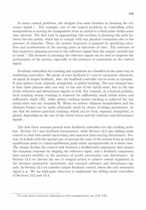
309
In many control problems, the designer has some freedom in choosing the ref-erence signal r. For example, one of the typical problems in controlling robotmanipulators is moving the manipulator from an initial to a final point within sometime interval. The first task in approaching this problem is planning the path be-tween the two points, which has to comply with any physical constraints due to thepresence of obstacles. Then, the motion trajectory is planned by specifying veloc-ities and accelerations of the moving parts as functions of time. The outcome ofthis trajectory planning process is the reference signal that the output variable hasto track.1 The freedom in choosing the reference signal can be used to improve theperformance of the system, especially in the presence of constraints on the controlsignal.
Feedback controllers for tracking and regulation are classified in the same way asstabilizing controllers. We speak of state feedback if x can be measured; otherwise,we speak of output feedback. Also, the feedback controller can be static or dynamic.It may achieve local, regional, semiglobal, or global tracking. The new element hereis that these phrases refer not only to the size of the initial state, but to the sizeof the reference and disturbance signals as well. For example, in a typical problem,local tracking means tracking is achieved for sufficiently small initial states andsufficiently small ‖R‖, while global tracking means tracking is achieved for anyinitial state and any bounded R. When we achieve ultimate boundedness and theultimate bound can be made arbitrarily small by choice of design parameters, wesay that we achieve practical tracking, which can be local, regional, semiglobal, orglobal, depending on the size of the initial states and the reference and disturbancesignals.
The first three sections present state feedback controllers for the tracking prob-lem. Section 13.1 uses feedback linearization, while Section 13.2 uses sliding modecontrol to deal with model uncertainty and matched time-varying disturbance. Sec-tion 13.3 deals with the special case of moving the state of the system from an initialequilibrium point to a final equilibrium point either asymptotically or in finite time.The design divides the control task between a feedforward component that shapesthe transient response by shaping the reference input, and a feedback componentthat ensures stability in the presence of model uncertainty and disturbance. InSection 13.4 we discuss the use of integral action to achieve robust regulation inthe presence parametric uncertainty and constant reference and disturbance sig-nals. In Section 13.5 we consider output feedback control, where the only measuredsignal is y. We use high-gain observers to implement the sliding mode controllersof Sections 13.2 and 13.4.
1To read about trajectory planning in robot manipulators, see [119, 135].
310 CHAPTER 13. TRACKING AND REGULATION
13.1 Tracking
Rewrite the system (13.6)–(13.8) as
η = f0(η, ξ), e = Ace + Bc
[a(η, ξ) + b(η, ξ)u − r(ρ)
]where ξ = e + R and the pair (Ac, Bc) represents a chain of ρ integrators. Byfeedback linearization,
u =[−a(η, ξ) + r(ρ) + v
]/b(η, ξ)
reduces the system to the cascade connection
η = f0(η, ξ), e = Ace + Bcv
The e-equation is stabilized by v = −Ke, where Ac−BcK is Hurwitz. The completestate feedback control is given by
u =[−a(η, ξ) + r(ρ) − Ke
]/b(η, ξ) (13.9)
and the closed-loop system is
η = f0(η, ξ), e = (Ac − BcK)e (13.10)
Since Ac − BcK is Hurwitz, e(t) is bounded and limt→∞ e(t) = 0. Consequently,ξ = e + R is bounded and, by Assumption 13.2, η is bounded.
Example 13.1 Consider the pendulum equation (A.2):
x1 = x2, x2 = − sin x1 − bx2 + cu, y = x1
The system has relative degree two in R2 and is in the normal form. It has no zerodynamics. We want the output y to track a reference signal r(t), with boundedderivatives r(t) and r(t). Taking
e1 = x1 − r, e2 = x2 − r
we obtaine1 = e2, e2 = − sin x1 − bx2 + cu − r
The state feedback control (13.9) is given by
u =1c[sin x1 + bx2 + r − k1e1 − k2e2]
where K = [k1, k2] assigns the eigenvalues of Ac − BcK at desired locations inthe open left-half complex plane. Because all the assumptions hold globally, this
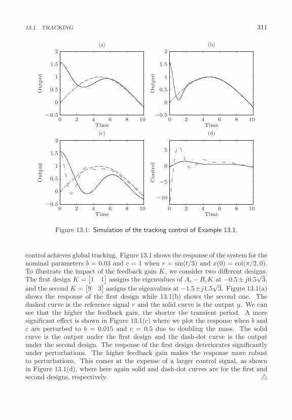
13.1. TRACKING 311
0 2 4 6 8 10−0.5
0
0.5
1
1.5
2
Time
Outp
ut
0 2 4 6 8 10−0.5
0
0.5
1
1.5
2
Time
Outp
ut
0 2 4 6 8 10−0.5
0
0.5
1
1.5
2
Time
Outp
ut
0 2 4 6 8 10
−10
−5
0
5
Time
Contr
ol
(c)
(a) (b)
(d)
Figure 13.1: Simulation of the tracking control of Example 13.1.
control achieves global tracking. Figure 13.1 shows the response of the system for thenominal parameters b = 0.03 and c = 1 when r = sin(t/3) and x(0) = col(π/2, 0).To illustrate the impact of the feedback gain K, we consider two different designs.The first design K =
[1 1
]assigns the eigenvalues of Ac −BcK at −0.5± j0.5
√3,
and the second K =[9 3
]assigns the eigenvalues at −1.5±j1.5
√3. Figure 13.1(a)
shows the response of the first design while 13.1(b) shows the second one. Thedashed curve is the reference signal r and the solid curve is the output y. We cansee that the higher the feedback gain, the shorter the transient period. A moresignificant effect is shown in Figure 13.1(c) where we plot the response when b andc are perturbed to b = 0.015 and c = 0.5 due to doubling the mass. The solidcurve is the output under the first design and the dash-dot curve is the outputunder the second design. The response of the first design deteriorates significantlyunder perturbations. The higher feedback gain makes the response more robustto perturbations. This comes at the expense of a larger control signal, as shownin Figure 13.1(d), where here again solid and dash-dot curves are for the first andsecond designs, respectively.
312 CHAPTER 13. TRACKING AND REGULATION
13.2 Robust Tracking
The system
η = f0(η, ξ)ei = ei+1, 1 ≤ i ≤ ρ − 1eρ = a(η, ξ) + b(η, ξ)u + δ(t, η, ξ, u) − r(ρ)(t)
is a perturbation of (13.6)–(13.8) that contains the matched time-varying distur-bance δ, which is assumed to be piecewise continuous in t and locally Lipschitz in(η, ξ, u). We may also allow uncertainty in the functions f0, a and b as long as As-sumptions 13.1 and 13.2 are satisfied. We design a state feedback controller usingsliding mode control. The e-equation is in the regular form (10.4). To design thesliding manifold, we start with the system
ei = ei+1, 1 ≤ i ≤ ρ − 1
where eρ is viewed as the control input, and design eρ to stabilize the origin. Forthis linear (controllable canonical form) system, we can achieve this task by thelinear control
eρ = −(k1e1 + · · · + kρ−1eρ−1)
where k1 to kρ−1 are chosen such that the polynomial
λρ−1 + kρ−1λρ−2 + · · · + k1
is Hurwitz. Then, the sliding manifold is taken as
s = (k1e1 + · · · + kρ−1eρ−1) + eρ = 0
and
s =ρ−1∑i=1
kiei+1 + a(η, ξ) + b(η, ξ)u + δ(t, η, ξ, u) − r(ρ)(t)
The control u can be taken as
u = v or u = − 1
b(η, ξ)
[ρ−1∑i=1
kiei+1 + a(η, ξ) − r(ρ)(t)
]+ v (13.11)
where in the second case we cancel the known terms on the right-hand side of thes-equation. The functions a and b are nominal models of a and b, respectively.When a = a and b = b, the term
−[a(η, ξ) − r(ρ)(t)
]/b(η, ξ)
13.2. ROBUST TRACKING 313
is the feedback linearizing term we used in the previous section. In either case, thes-equation can be written as
s = b(η, ξ)v + Δ(t, η, ξ, v)
Suppose ∣∣∣∣Δ(t, η, ξ, v)b(η, ξ)
∣∣∣∣ ≤ �(η, ξ) + κ0|v|, 0 ≤ κ0 < 1
for all t ≥ 0, v ∈ R, and (η, ξ) ∈ Dη × Dξ, where � and κ0 are known. Then,
v = −β(η, ξ) sat(s/μ) (13.12)
where β(η, ξ) is a locally Lipschitz function that satisfies
β(η, ξ) ≥ �(η, ξ)/(1 − κ0) + β0, with β0 > 0
ensures that ss ≤ −β0b0(1 − κ0)|s| for |s| ≥ μ. Due to Assumption 13.2, we focusour attention on the behavior of e(t). Setting ζ = col(e1, . . . , eρ−1), it can be seenthat ζ satisfies the equation
ζ = (Ac − BcK)ζ + Bcs
where K =[k1 k2 . . . kρ−1
]and the pair (Ac, Bc) represents a chain of (ρ− 1)
integrators. The matrix Ac − BcK is Hurwitz by design. Let P be the solution ofthe Lyapunov equation P (Ac − BcK) + (Ac − BcK)T P = −I. The derivative ofV0 = ζT Pζ satisfies the inequality
V0 = −ζT ζ + 2ζT PBcs ≤ −(1 − θ)‖ζ‖2, ∀ ‖ζ‖ ≥ 2‖PBc‖ |s|/θ
where 0 < θ < 1. Since ζT Pζ ≤ λmax(P )‖ζ‖2, for any σ ≥ μ
{‖ζ‖ ≤ 2‖PBc‖ σ/θ} ⊂ {ζT Pζ ≤ λmax(P )(2‖PBc‖/θ)2σ2}Set ρ1 = λmax(P )(2‖PBc‖/θ)2 and choose c > μ such that Ω = {ζT Pζ ≤ ρ1c
2} ×{|s| ≤ c} is in the domain of interest. The set Ω is positively invariant because ss < 0on the boundary {|s| = c} and V0 < 0 on the boundary {V0 = ρ1c
2}. Let e(0) ∈ Ω.Within finite time, e(t) enters the set Ωμ = {ζT Pζ ≤ ρ1μ
2}×{|s| ≤ μ}, which is alsopositively invariant. Inside Ωμ, we can use (B.4) to show that maxζT Pζ≤ρ1μ2 |e1| =√
ρ1μ2‖LP−1/2‖, where L =[1 0 . . . 0
]. Setting k = ‖LP−1/2‖√ρ1 shows
that the ultimate bound on |e1| is kμ.
Example 13.2 Reconsider the pendulum tracking problem from Example 13.1:
e1 = e2, e2 = − sin x1 − bx2 + cu − r
where r(t) = sin(t/3), and suppose that b and c are uncertain parameters thatsatisfy 0 ≤ b ≤ 0.1 and 0.5 ≤ c ≤ 2. Taking s = e1 + e2, we have
s = e2 − sinx1 − bx2 + cu − r = (1 − b)e2 − sin x1 − br − r
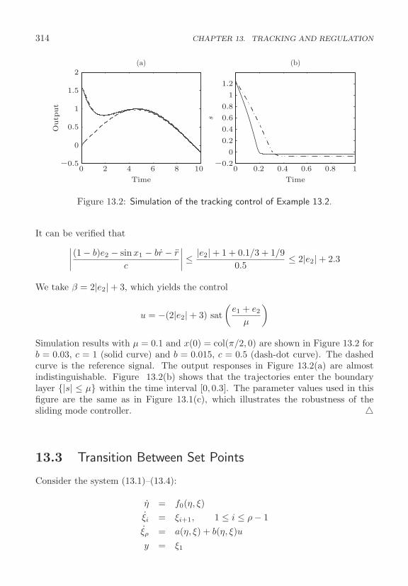
314 CHAPTER 13. TRACKING AND REGULATION
0 2 4 6 8 10−0.5
0
0.5
1
1.5
2
0 0.2 0.4 0.6 0.8 1−0.2
0
0.2
0.4
0.6
0.8
1
1.2
Time Time
Outp
ut
s
(a) (b)
Figure 13.2: Simulation of the tracking control of Example 13.2.
It can be verified that∣∣∣∣ (1 − b)e2 − sin x1 − br − r
c
∣∣∣∣ ≤ |e2| + 1 + 0.1/3 + 1/90.5
≤ 2|e2| + 2.3
We take β = 2|e2| + 3, which yields the control
u = −(2|e2| + 3) sat(
e1 + e2
μ
)
Simulation results with μ = 0.1 and x(0) = col(π/2, 0) are shown in Figure 13.2 forb = 0.03, c = 1 (solid curve) and b = 0.015, c = 0.5 (dash-dot curve). The dashedcurve is the reference signal. The output responses in Figure 13.2(a) are almostindistinguishable. Figure 13.2(b) shows that the trajectories enter the boundarylayer {|s| ≤ μ} within the time interval [0, 0.3]. The parameter values used in thisfigure are the same as in Figure 13.1(c), which illustrates the robustness of thesliding mode controller.
13.3 Transition Between Set Points
Consider the system (13.1)–(13.4):
η = f0(η, ξ)ξi = ξi+1, 1 ≤ i ≤ ρ − 1ξρ = a(η, ξ) + b(η, ξ)uy = ξ1
13.3. TRANSITION BETWEEN SET POINTS 315
where Assumptions 13.1 and 13.2 are satisfied over the domain of interest. For aconstant input u, the equilibrium point (η, ξ) satisfies the equations
0 = f0(η, ξ)0 = ξi+1, 1 ≤ i ≤ ρ − 10 = b(η, ξ) + a(η, ξ)uy = ξ1
Therefore, ξ = col(y, 0, · · · , 0). Assume that
0 = f0(η, ξ)
has a unique solution η in the domain of interest; denote it by η = φη(y). Moreover,assume that η is an asymptotically stable equilibrium point of η = f0(η, ξ) (aminimum phase property). Because b(η, ξ) �= 0, u is given by
u = − a(η, ξ)b(η, ξ)
def= φu(y)
Thus, to maintain the output at a constant value y, we need to maintain the systemat the equilibrium point η = φη(y) and ξ = col(y, 0, · · · , 0), using the constantcontrol u = φu(y). For each y there is a unique triple (η, ξ, u). Without loss ofgenerality we assume that φη(0) = 0 and φu(0) = 0.
Suppose now we want to move the system from equilibrium at y = 0 to equilib-rium at y = y∗. This task can be cast as a tracking problem by taking the referencesignal as
r = y∗ and r(i) = 0 for i ≥ 1
for which the initial state e(0) = col(−y∗, 0, . . . , 0). Shaping the transient responseof e(t) is straightforward when a and b are known and the linearizing feedbackcontrol
u =−a(η, ξ) − Ke
b(η, ξ)
is used because e(t) satisfies the equation e = (Ac−BcK)e, whose transient responsecan be shaped by assignment of the eigenvalues of Ac − BcK. When a and b areperturbed, the transient response will deviate from the solution of e = (Ac−BcK)e.To cope with uncertainty, we can use the sliding mode controller of the previoussection, but shaping the transient response will be more involved because duringthe reaching phase s satisfies a nonlinear equation.
An alternative approach that enables us to shape the transient response is tochoose the reference r(t) as a smooth signal with r and its derivatives r(1) to r(ρ−1)
all starting from zero at t = 0. Then, r(t) approaches y∗, with its derivativesapproaching zero, either asymptotically or over a finite period time. Because rand its derivatives are zero at t = 0, the initial vector e(0) = 0. In the case of
316 CHAPTER 13. TRACKING AND REGULATION
feedback linearization with no uncertainty, e(0) = 0 implies that e(t) ≡ 0 becausee satisfies the equation e = (Ac − BcK)e. Therefore y(t) ≡ r(t) for all t ≥ 0.In the case of sliding mode control, it is shown in the previous section that the setΩμ = {ζT Pζ ≤ ρ1μ
2}×{|s| ≤ μ} is positively invariant, where ζ = col(e1, . . . , eρ−1)and s = k1e1 + · · · + kρ−1eρ−1 + eρ. Because 0 ∈ Ωμ,
e(0) = 0 ⇒ e(0) ∈ Ωμ ⇒ e(t) ∈ Ωμ, ∀ t ≥ 0
Hence, y(t) will be within O(μ) neighborhood of r(t) for all t ≥ 0.The reference r(t) can be shaped to achieve the desired transient response. For
example, r(t) can be taken as the zero-state response of the Hurwitz transfer func-tion
aρ
sρ + a1sρ−1 + · · · + aρ−1s + aρ
with a step input of amplitude y∗. The positive constants a1 to aρ are chosen toshape the response of r. A state-space realization of this transfer function is
z =
⎡⎢⎢⎢⎣
1. . .
1−aρ −a1
⎤⎥⎥⎥⎦ z +
⎡⎢⎢⎣
aρ
⎤⎥⎥⎦ y∗
r =[
1]z
By taking z(0) = 0 we enforce the condition that the initial values of r and itsderivatives up to r(ρ−1) are all zero. As time approaches infinity, r(t) approachesy∗ while its derivatives approach zero.
Another approach is to plan the trajectory (r(t), r(t), . . . , r(ρ−1)(t)) to movefrom (0, 0, . . . , 0) to (y∗, 0, . . . , 0) in finite time T . Figure 13.3 shows an examplewhen ρ = 2. For this example,
r(t) =
⎧⎪⎨⎪⎩
at2
2 for 0 ≤ t ≤ T2
−aT 2
4 + aT t − at2
2 for T2 ≤ t ≤ T
aT 2
4 for t ≥ T
Taking a = 4y∗/T 2 ensures that r(t) = y∗ for t ≥ T . In this case, there is animportant difference between the case with no zero dynamics and the one withasymptotically stable zero dynamics. When there are no zero dynamics, the inputu reaches φu(y∗) during the finite period T . When there are zero dynamics, the ηvariables will continue to move beyond the period T . In this case η(t) and u(t) willasymptotically approach their equilibrium values φη(y∗) and φu(y∗).
The freedom in choosing the reference signal r to move y from zero to y∗ canbe used to deal with control constraints.2 It is clear that aggressively moving the
2See [24, 50, 64] for techniques that take control constraints into consideration.
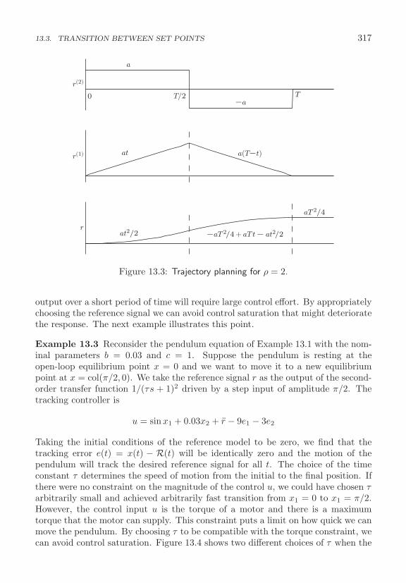
13.3. TRANSITION BETWEEN SET POINTS 317
TT/20
a
−a
r(2)
r(1) at
at2/2
aT 2/4
r
a(T−t)
−aT 2/4 + aT t− at2/2
Figure 13.3: Trajectory planning for ρ = 2.
output over a short period of time will require large control effort. By appropriatelychoosing the reference signal we can avoid control saturation that might deterioratethe response. The next example illustrates this point.
Example 13.3 Reconsider the pendulum equation of Example 13.1 with the nom-inal parameters b = 0.03 and c = 1. Suppose the pendulum is resting at theopen-loop equilibrium point x = 0 and we want to move it to a new equilibriumpoint at x = col(π/2, 0). We take the reference signal r as the output of the second-order transfer function 1/(τs + 1)2 driven by a step input of amplitude π/2. Thetracking controller is
u = sin x1 + 0.03x2 + r − 9e1 − 3e2
Taking the initial conditions of the reference model to be zero, we find that thetracking error e(t) = x(t) − R(t) will be identically zero and the motion of thependulum will track the desired reference signal for all t. The choice of the timeconstant τ determines the speed of motion from the initial to the final position. Ifthere were no constraint on the magnitude of the control u, we could have chosen τarbitrarily small and achieved arbitrarily fast transition from x1 = 0 to x1 = π/2.However, the control input u is the torque of a motor and there is a maximumtorque that the motor can supply. This constraint puts a limit on how quick we canmove the pendulum. By choosing τ to be compatible with the torque constraint, wecan avoid control saturation. Figure 13.4 shows two different choices of τ when the

318 CHAPTER 13. TRACKING AND REGULATION
0 1 2 3 4 50
0.5
1
1.5
2
Outp
ut
output
reference
0 1 2 3 4 50
0.5
1
1.5
2
Outp
ut
output
reference
0 1 2 3 4 5
−2
−1
0
1
2
Time
Contr
ol
0 1 2 3 4 5
−2
−1
0
1
2
Time
Contr
ol
τ = 0.2 τ = 0.8
τ = 0.2 τ = 0.8
Figure 13.4: Simulation of the tracking control of Example 13.3.
control is constrained to |u| ≤ 2. For τ = 0.2, the control saturates during the initialtransient causing the output y(t) to deviate from the reference r(t), which reflectsthe fact that the reference signal demands a control effort that cannot be deliveredby the motor. On the other hand, with τ = 0.8, the output signal achieves goodtracking of the reference signal. In both cases, we could not achieve a settling timebetter than about 4, but by choosing τ = 0.8, we were able to avoid the overshootthat took place when τ = 0.2.
13.4 Robust Regulation via Integral Action
The system
η = f0(η, ξ, w) (13.13)ξi = ξi+1, 1 ≤ i ≤ ρ − 1 (13.14)ξρ = a(η, ξ, w) + b(η, ξ, w)u (13.15)y = ξ1 (13.16)

13.4. ROBUST REGULATION VIA INTEGRAL ACTION 319
is a perturbation of (13.1)–(13.4) where w ∈ Dw ⊂ R� is a vector of unknownconstant parameters and disturbances defined over some domain Dw. We assumethat Assumptions 13.1 and 13.2 hold for all w ∈ Dw with b0 independent of w. Ourgoal is to design a state feedback controller such that all state variables are boundedand the output y is asymptotically regulated to a constant reference r ∈ Dr ⊂ R,for some domain Dr. This is a special case of the tracking problem of Section 13.2,where the reference is constant and the uncertainty is parameterized by w. Thesliding mode controller of Section 13.2 will ensure that the regulation error y − rwill be ultimately bounded by kμ for some k > 0. By using integral action, we canensure that the error will converge to zero as time tends to infinity. The controllerwill drive the trajectory to an equilibrium point (η, ξ) that satisfies the equations
0 = f0(η, ξ, w)0 = ξi+1, 1 ≤ i ≤ ρ − 10 = a(η, ξ, w) + b(η, ξ, w)ur = ξ1
Hence, ξ = col(r, 0, . . . , 0).
Assumption 13.5 For all (r, w) ∈ Dr × Dw, the equation 0 = f0(η, ξ, w) has aunique solution η ∈ Dη, which we denote by η = φη(r, w).
Because b �= 0, the steady-state control needed to maintain this equilibrium pointis given by
u = − a(η, ξ, w)b(η, ξ, w)
def= φu(r, w)
Augmenting the integratore0 = y − r (13.17)
with the system and applying the change of variables
z = η − η, e =
⎡⎢⎢⎢⎣
e1
e2
...eρ
⎤⎥⎥⎥⎦ =
⎡⎢⎢⎢⎣
ξ1 − rξ2
...ξρ
⎤⎥⎥⎥⎦
we obtain the augmented system
z = f0(z + η, ξ, w) def= f0(z, e, r, w)ei = ei+1, for 0 ≤ i ≤ ρ − 1eρ = a(η, ξ, w) + b(η, ξ, w)u
which preserves the normal form structure with a chain of ρ+1 integrators. There-fore, the design of sliding mode control can proceed as in Section 13.2. We take
s = k0e0 + k1e1 + · · · + kρ−1eρ−1 + eρ
320 CHAPTER 13. TRACKING AND REGULATION
where k0 to kρ−1 are chosen such that the polynomial
λρ + kρ−1λρ−1 + · · · + k1λ + k0
is Hurwitz. Then,
s =ρ−1∑i=0
kiei+1 + a(η, ξ, w) + b(η, ξ, w)u
The control u can be taken as
u = v or u = − 1
b(η, ξ)
[ρ−1∑i=0
kiei+1 + a(η, ξ)
]+ v (13.18)
where a and b are nominal models of a and b, respectively. Then,
s = b(η, ξ, w)v + Δ(η, ξ, r, w)
If ∣∣∣∣Δ(η, ξ, r, w)b(η, ξ, w)
∣∣∣∣ ≤ �(η, ξ)
for all (η, ξ, r, w) ∈ Dη ×Dξ ×Dr ×Dw, with a known locally Lipschitz function �,we take
v = −β(η, ξ) sat(
s
μ
)(13.19)
where β(η, ξ) is a locally Lipschitz function that satisfies β(η, ξ) ≥ �(η, ξ)+β0 withβ0 > 0. The closed-loop system has an equilibrium point at (z, e0, e) = (0, e0, 0).Showing convergence to this equilibrium point can be done by analysis similar tothe analysis of Section 10.1, under the following two assumptions.
Assumption 13.6 For all (r, w) ∈ Dr×Dw, there is a Lyapunov function V1(z, r, w)for the system z = f0(z, e, r, w) that satisfies the inequalities
α1(‖z‖) ≤ V1(z, r, w) ≤ α2(‖z‖)∂V1
∂zf0(z, e, r, w) ≤ −α3(‖z‖), ∀ ‖z‖ ≥ α4(‖e‖)
for some class K functions α1 to α4.
Assumption 13.7 z = 0 is an exponentially stable equilibrium point of the systemz = f0(z, 0, r, w).
The convergence of the error to zero is stated in the following theorem whoseproof is given in Appendix D.

13.4. ROBUST REGULATION VIA INTEGRAL ACTION 321
Theorem 13.1 Suppose Assumptions 13.1, 13.2, 13.5, 13.6 and 13.7 are satisfiedfor the system (13.13)–(13.16) and consider the controller (13.17)–(13.19). Then,there are positive constants c, ρ1 and ρ2 and a positive definite matrix P such thatthe set
Ω = {V1(z) ≤ α2(α4(cρ2)} × {ζT Pζ ≤ ρ1c2} × {|s| ≤ c}
where ζ = col(e0, e1, . . . , eρ−1), is compact and positively invariant, and for allinitial states in Ω, limt→∞ |y(t) − r| = 0. �
In the special case when β = k (a constant) and u = v, the controller is givenby
u = −k sat(
k0e0 + k1e1 + · · · + kρ−1eρ−1 + eρ
μ
)(13.20)
When ρ = 1 the controller (13.20) is a classical PI (Proportional-Integral) controllerfollowed by saturation and when ρ = 2 it is a classical PID (Proportional-Integral-Derivative) controller followed by saturation.
Example 13.4 Consider the pendulum equation (A.2) and suppose that the sus-pension point is subjected to a constant horizontal acceleration. The state modelis given by
x1 = x2, x2 = − sin x1 − bx2 + cu + d cos x1, y = x1
It is desired to regulate y to a constant reference r. Suppose b, c, d are uncertainparameters that satisfy 0 ≤ b ≤ 0.1, 0.5 ≤ c ≤ 2, and 0 ≤ d ≤ 0.5. Definee1 = x1 − r, e2 = x2, and augment the integrator e0 = e1 with the system to obtain
e0 = e1, e1 = e2, e2 = − sin x1 − bx2 + cu + d cos x1
Taking s = e0 + 2e1 + e2, assigns the eigenvalues of λ2 + 2λ + 1 at −1, −1. Thederivative s is given by
s = e1 + (2 − b)e2 − sinx1 + cu + d cos x1
It can be verified that∣∣∣∣e1 + (2 − b)e2 − sin x1 + d cos x1
c
∣∣∣∣ ≤ |e1| + 2|e2| + 1 + 0.50.5
= 2|e1| + 4|e2| + 3
We take β = 2|e1| + 4|e2| + 4, which yields the control
u = −(2|e1| + 4|e2| + 4) sat(
e0 + 2e1 + e2
μ
)For comparison, we design also a sliding mode controller without integral action,where s = e1 + e2 and
s = (1 − b)e2 − sin x1 + cu + d cos x1
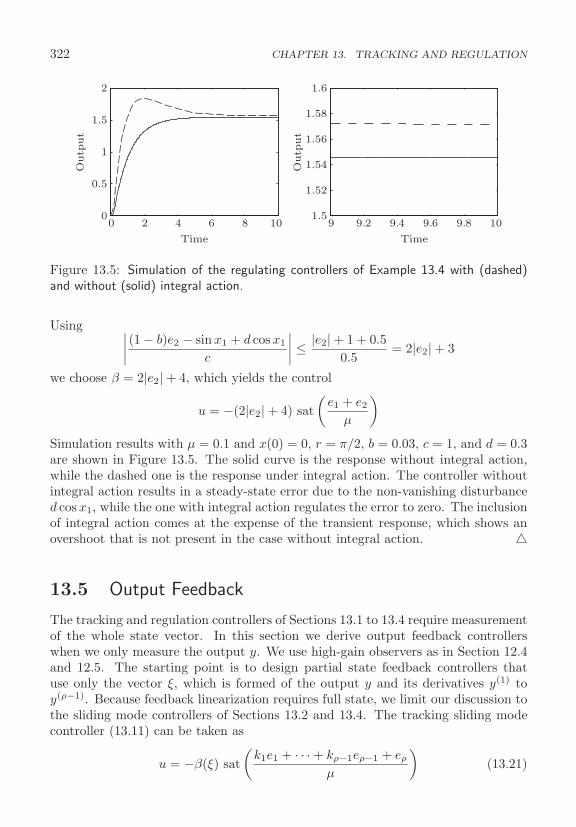
322 CHAPTER 13. TRACKING AND REGULATION
0 2 4 6 8 100
0.5
1
1.5
2
Time
Outp
ut
9 9.2 9.4 9.6 9.8 101.5
1.52
1.54
1.56
1.58
1.6
Time
Outp
ut
Figure 13.5: Simulation of the regulating controllers of Example 13.4 with (dashed)and without (solid) integral action.
Using ∣∣∣∣ (1 − b)e2 − sin x1 + d cos x1
c
∣∣∣∣ ≤ |e2| + 1 + 0.50.5
= 2|e2| + 3
we choose β = 2|e2| + 4, which yields the control
u = −(2|e2| + 4) sat(
e1 + e2
μ
)Simulation results with μ = 0.1 and x(0) = 0, r = π/2, b = 0.03, c = 1, and d = 0.3are shown in Figure 13.5. The solid curve is the response without integral action,while the dashed one is the response under integral action. The controller withoutintegral action results in a steady-state error due to the non-vanishing disturbanced cos x1, while the one with integral action regulates the error to zero. The inclusionof integral action comes at the expense of the transient response, which shows anovershoot that is not present in the case without integral action.
13.5 Output Feedback
The tracking and regulation controllers of Sections 13.1 to 13.4 require measurementof the whole state vector. In this section we derive output feedback controllerswhen we only measure the output y. We use high-gain observers as in Section 12.4and 12.5. The starting point is to design partial state feedback controllers thatuse only the vector ξ, which is formed of the output y and its derivatives y(1) toy(ρ−1). Because feedback linearization requires full state, we limit our discussion tothe sliding mode controllers of Sections 13.2 and 13.4. The tracking sliding modecontroller (13.11) can be taken as
u = −β(ξ) sat(
k1e1 + · · · + kρ−1eρ−1 + eρ
μ
)(13.21)
13.5. OUTPUT FEEDBACK 323
The regulation sliding mode controller (13.18) can be taken as
u = −β(ξ) sat(
k0e0 + k1e1 + · · · + kρ−1eρ−1 + eρ
μ
)(13.22)
where e0 = e1 = y − r. The main restriction here is that β is allowed to dependonly on ξ rather than the full state vector. Because β is chosen to dominate afunction �(η, ξ), this restriction may force us to limit the analysis to a compact setover which the η-dependent part of �(η, ξ) can be bounded by a constant. In theoutput feedback case, we use the high-gain observer
˙ei = ei+1 +αi
εi(y − r − e1), 1 ≤ i ≤ ρ − 1 (13.23)
˙eρ =αρ
ερ(y − r − e1) (13.24)
to estimate e by e, where ε is a sufficiently small positive constant and α1 to αρ arechosen such that the polynomial
λρ + α1λρ−1 + · · · + αρ−1λ + αρ (13.25)
is Hurwitz. The estimate ξ is given by ξ = e + R. To overcome the peaking phe-nomenon of high-gain observers, the control should be a globally bounded functionof e. Because the saturation function is bounded, we only need to saturate β(ξ)outside a compact set of interest. Denote the saturated function by βs(ξ). Then,the output feedback tracking controller is given by
u = −βs(ξ) sat(
k1e1 + · · · + kρ−1eρ−1 + eρ
μ
)(13.26)
while the output feedback regulation controller is given by
u = −βs(ξ) sat(
k0e0 + k1e1 + · · · + kρ−1eρ−1 + eρ
μ
)(13.27)
Note that the integrator state e0 is available because it is obtained by integratingthe regulation error e1 = y − r. In both (13.26) and (13.27), we can replace e1
by the measured signal e1. In the special case when βs of (13.26) is constant orfunction of e rather than ξ, we do not need the derivatives of r, as required byAssumption 13.4, because e is provided by the observer (13.23)–(13.24), which isdriven by y − r; so only r is needed.
Similar to the results of Sections 12.4 and 12.5, it can be shown that the outputfeedback controllers (13.26) and (13.27) recover the performance of the partial statefeedback controllers (13.21) and (13.22), respectively, for sufficiently small ε. In theregulation case, it can be shown that the regulation error converges to zero.3
3The proof for a slightly modified problem formulation can be found in [73].
324 CHAPTER 13. TRACKING AND REGULATION
For relative degree one systems, the controllers (13.21) and (13.22) are given by
u = −β(y) sat(
y − r
μ
)and u = −β(y) sat
(k0e0 + y − r
μ
)
respectively, where e0 = y − r. These controllers depend only on the measuredoutput y; hence, no observer is needed.
Example 13.5 We use the high-gain observer
˙e1 = e2 +2ε(e1 − e1), ˙e2 =
1ε2
(e1 − e1)
to implement the tracking controller
u = −(2|e2| + 3) sat(
e1 + e2
μ
)
of Example 13.2 and the regulating controller
u = −(2|e1| + 4|e2| + 4) sat(
e0 + 2e1 + e2
μ
)
of Example 13.4. We use e2 from the observer to replace e2 but keep e1 since itis a measured signal. To overcome the observer peaking, we saturate |e2| in theβ function over a compact set of interest. There is no need to saturate e2 insidethe saturation because the saturation function is globally bounded. We use theanalysis of the state feedback controller to determine the compact set of interest.For the tracking controller of Example 13.2, the analysis of Section 13.2 shows thatΩ = {|e1| ≤ c/θ} × {|s| ≤ c}, with c > 0 and 0 < θ < 1, is positively invariant.Taking c = 2 and 1/θ = 1.1, we obtain Ω = {|e1| ≤ 2.2} × {|s| ≤ 2}. Over Ω,|e2| ≤ |e1|+ |s| ≤ 4.2. We saturate |e2| at 4.5, which results in the output feedbackcontroller
u = −(
2 × 4.5 sat( |e2|
4.5
)+ 3)
sat(
e1 + e2
μ
)For the regulating controller of Example 13.4, ζ = col(e0, e1) satisfies the equation
ζ = Aζ + Bs, where A =[
0 1−1 −2
]and B =
[01
]
From the proof of Theorem 13.1 in Appendix D, it can be seen that Ω = {ζT Pζ ≤ρ1c
2} × {|s| ≤ c} is positively invariant, where c > 0, P is the solution of theLyaunov equation PA + AT P = −I, ρ1 = λmax(P )(2‖PB‖/θ)2, and 0 < θ < 1.Taking c = 4 and 1/θ = 1.003, we obtain Ω = {ζT Pζ ≤ 55} × {|s| ≤ 4}. Using(B.4), it can be shown that over Ω, |e0 + 2e1| ≤ √
55 ‖ [1 2]P−1/2‖ = 22.25;

13.6. EXERCISES 325
0 1 2 3 4
0.6
0.8
1
1.2
1.4
1.6
Time
Outp
ut
(a)
0 2 4 60
0.5
1
1.5
2
Time
Outp
ut
(b)
Figure 13.6: Simulation of the output feedback controllers of Example 13.5, comparingthe response under state feedback (solid) with the one under output feedback whenε = 0.05 (dashed) and ε = 0.01 (dash-dot).
consequently, |e2| ≤ |e0 + 2e1| + |s| ≤ 26.25. We saturate |e2| at 27, which resultsin the output feedback controller
u = −(
2|e1| + 4 × 27 sat( |e2|
27
)+ 4)
sat(
e0 + 2e1 + e2
μ
)
The simulation results of Figure 13.6 use the same data of Examples 13.2 and 13.4with two different values of ε, 0.05 and 0.01. Figure 13.6(a) is for the trackingcontroller of Example 13.2 and Figure 13.6(b) for the regulating controller of Ex-ample 13.4. In both cases, the solid curve is for state feedback and the other twocurves are for output feedback with ε = 0.05 (dashed curve) and ε = 0.01 (dash-dotcurve). As we have seen before with high-gain observers, the response under outputfeedback approaches the one under state feedback as the ε decreases.
13.6 Exercises
13.1 Consider a tracking problem for the magnetic levitation system (A.30)–(A.32) where y = x1, r(t) = 0.5 sin ωt, α = 1.5, β = 2, b = 0, and c = 1.
(a) Design a state feedback controller using feedback linearization. Using simula-tion with ω = 1, choose the controller parameters to have settling time lessthan 20 time units.
(b) Design an observer to implement the controller of part (a) assuming you mea-sure x1 and x3. Use simulation, with ω = 1, x(0) = col(1, 0, 1), and x(0) = 0,to compare the performance of the state and output feedback controllers.
326 CHAPTER 13. TRACKING AND REGULATION
(c) Repeat (b) assuming you can only measure x1.
13.2 Repeat the previous exercise when the reference signal is taken as r(t) =r0 + (r1 − r0)q(t), where q(3)(t) is defined by
q(3)(t) =
⎧⎪⎪⎨⎪⎪⎩
1/2 for 0 ≤ t < 1−1/2 for 1 ≤ t < 3
1/2 for 3 ≤ t < 40 for t ≥ 4
and q(0) = q(0) = q(0) = 0, which is chosen to steer the system from equilibriumat x1 = r0 to equilibrium at x1 = r1 over four time units. In the simulation taker0 = 1, r1 = 2, and x(0) = col(1, 0, 1).
13.3 Reconsider the previous exercise when c ∈ [0.5, 1.5] is uncertain and theonly available signal is the tracking error x1 − r. Using sliding mode control anda high-gain observer, design a locally Lipschitz feedback controller. What is thesteady-state tracking error? Simulate the response for different values of c. Hint:The controller can take the form u = K sat((K1e1 + K2e2 + e3)/μ) where e1, e2,and e3 are estimates of the tracking error e1 = x1 − r and its derivatives e2 = e1
and e3 = e1, respectively.
13.4 Repeat the previous exercise using integral action.
13.5 Consider a tracking problem for the electrostatic microactuator (A.33) wherer(t) = r0 + (r1 − r0)q(t) and q(t) is the output of the transfer function 1/(s + 1)3
with a unit step input. The reference r(t) is chosen to steer x1 from equilibrium atr0 > 0 to equilibrium at r1 > 0.
(a) Design a locally Lipschitz state feedback controller using feedback linearization.Simulate the closed-loop system with ζ = 0.1, T = 0.2, r0 = 0.1, r1 = 0.5,and x(0) = col(0.1, 0,
√0.3).
(b) Design an observer to implement the controller of part (a) assuming you mea-sure x1 and x3. Use simulation to compare the performance of the state andoutput feedback controllers.
(c) Repeat (b) assuming you can only measure x1.
13.6 Repeat the previous exercise using sliding mode control when ζ ∈ (0, 0.5] andT ∈ [0.1, 0.5] are uncertain parameters. What is the steady-state tracking error?
13.7 Repeat the previous exercise using integral action.
13.8 Consider the robot manipulator (A.34) and let M , C and g be nominalmodels of M , C, and g, respectively. We want to design a feedback controller suchthat q(t) asymptotically tracks a reference trajectory qr(t), where qr(t), qr(t), andqr(t) are continuous and bounded.

13.6. EXERCISES 327
(a) Design a locally Lipschitz state feedback controller to achieve global practicaltracking.
(b) Assuming you measure q but not q, design a locally Lipschitz output feedbackcontroller to achieve semiglobal practical tracking.
Hint: Assume appropriate bounds on the model uncertainty.
13.9 The tank system of Exercise 1.9 is modeled by
h =[u − k
√ρgh]/A(h)
Assume that A(h) ≤ c1 and k√
ρg ≤ c2 for known positive constants c1 and c2.Using sliding mode control, design a locally Lipschitz output feedback controllerthat regulates h to r with zero steady-state error.
13.10 Consider the DC motor(A.24) with ϑ = 0, nonlinear friction η(ω) = k1ω +k2 sgn(ω), and unknown positive constants a, k1, and k2. Assume that a ∈ [0.5, 1.5],k1 ≤ 0.1 and k2 ≤ 0.2. Design a locally Lipschitz output feedback controller toregulate ω to ω∗ with zero steady-state error.
13.11 A normalized model of a pendulum whose suspension point is subjected toa constant horizontal acceleration is given by
x1 = x2, x2 = − sin x1 − bx2 + cu + h
where 0 ≤ b ≤ 0.4, 0.5 ≤ c ≤ 1.5, and |h| ≤ 1.
(a) Design a locally Lipschitz state feedback controller to regulate x1 to zero withzero steady-state error.
(b) Repeat (a) if you can only measure x1.
13.12 Consider the magnetic levitation system (A.29) with uncertain parametersb ∈ [0, 0.1] and c ∈ [0.8, 1.2]. It is required to regulate x1 to r ∈ [0.5, 1.5] with zerosteady-state error, while meeting the constraint −2 ≤ u ≤ 0.
(a) Design a locally Lipschitz state feedback controller.
(b) Repeat (a) if you can only measure x1.
13.13 Consider the system y = f(y, y) + u, where f is unknown, locally Lipschitzfunction with f(0, 0) = 0, and the control u is constrained by |u| ≤ U for a givenconstant U . Suppose the system is initially at the equilibrium point (0, 0) and wewant y to track a reference signal r(t) with the properties: (1) r(t) has boundedcontinuous derivatives up to the second order; (2) maxt≥0 |r − f(r, r)| < U ; (3)r(0) = r(0) = 0.
328 CHAPTER 13. TRACKING AND REGULATION
(a) If the measurements of y, y, r, r, and r are available, design a locally Lipschitzfeedback controller such that |y(t) − r(t)| ≤ δ ∀ t ≥ 0 for a given δ.
(b) Repeat (a) if only the measurements of y and r are available.
13.14 A simplified model of an underwater vehicle in yaw is given by
ψ + aψ|ψ| = u
where ψ is the heading angle, u is a normalized torque, and a is a positive parameter.To move ψ from set point 0 to set point ψ∗, a reference signal is taken as ψr(t) =ψ∗[1 − e−t(1 + t)].
(a) With a = 1, use feedback linearization to design a state feedback controllersuch that ψ(t) ≡ ψr(t) for all t ≥ 0.
(b) Suppose a �= 1. Find an upper bound on |a − 1| such that the tracking errorunder the controller of part (a) converges to zero as t tends to infinity.
(c) Assuming |a − 1| ≤ 0.5, design a locally Lipschitz state feedback controller toachieve global asymptotic tracking.
(d) Assuming |a− 1| ≤ 0.5 and you can only measure ψ, design a locally Lipschitzoutput feedback controller to achieve semiglobal asymptotic tracking.
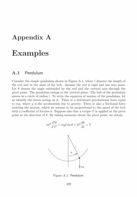
Appendix A
Examples
A.1 Pendulum
Consider the simple pendulum shown in Figure A.1, where l denotes the length ofthe rod and m the mass of the bob. Assume the rod is rigid and has zero mass.Let θ denote the angle subtended by the rod and the vertical axis through thepivot point. The pendulum swings in the vertical plane. The bob of the pendulummoves in a circle of radius l. To write the equation of motion of the pendulum, letus identify the forces acting on it. There is a downward gravitational force equalto mg, where g is the acceleration due to gravity. There is also a frictional forceresisting the motion, which we assume to be proportional to the speed of the bobwith a coefficient of friction k. Suppose also that a torque T is applied at the pivotpoint in the direction of θ. By taking moments about the pivot point, we obtain
ml2d2θ
d t2+ mgl sin θ + kl2
dθ
dt= T
θ
mg
l
Figure A.1: Pendulum.
329
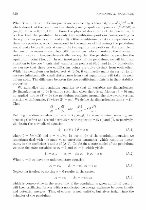
330 APPENDIX A. EXAMPLES
When T = 0, the equilibrium points are obtained by setting dθ/dt = d2θ/dt2 = 0,which shows that the pendulum has infinitely many equilibrium points at (θ, dθ/dt) =(nπ, 0), for n = 0,±1,±2, . . .. From the physical description of the pendulum, itis clear that the pendulum has only two equilibrium positions corresponding tothe equilibrium points (0, 0) and (π, 0). Other equilibrium points are repetitions ofthese two positions, which correspond to the number of full swings the pendulumwould make before it rests at one of the two equilibrium positions. For example, ifthe pendulum makes m complete 360◦ revolutions before it rests at the downwardvertical position, then, mathematically, we say that the pendulum approaches theequilibrium point (2mπ, 0). In our investigation of the pendulum, we will limit ourattention to the two “nontrivial” equilibrium points at (0, 0) and (π, 0). Physically,we can see that these two equilibrium points are quite distinct from each other.While the pendulum can indeed rest at (0, 0), it can hardly maintain rest at (π, 0)because infinitesimally small disturbance from that equilibrium will take the pen-dulum away. The difference between the two equilibrium points is in their stabilityproperties.
We normalize the pendulum equation so that all variables are dimensionless.By linearization at (0, 0) it can be seen that when there is no friction (k = 0) andno applied torque (T = 0) the pendulum oscillates around the downward verticalposition with frequency Ω where Ω2 = g/l. We define the dimensionless time τ = Ωt.Then
dθ
dt= Ω
dθ
dτand
d2θ
dt2= Ω2 d2θ
dτ2
Defining the dimensionless torque u = T/(mogl) for some nominal mass mo anddenoting the first and second derivatives with respect to τ by ˙(·) and (·), respectively,we obtain the normalized equation
θ + sin θ + b θ = c u (A.1)
where b = k/(mΩ) and c = mo/m. In our study of the pendulum equation wesometimes deal with the mass m as uncertain parameter, which results in uncer-tainty in the coefficient b and c of (A.1). To obtain a state model of the pendulum,we take the state variables as x1 = θ and x2 = θ, which yields
x1 = x2, x2 = − sin x1 − b x2 + c u (A.2)
When u = 0 we have the unforced state equation
x1 = x2, x2 = − sin x1 − b x2 (A.3)
Neglecting friction by setting b = 0 results in the system
x1 = x2, x2 = − sin x1 (A.4)
which is conservative in the sense that if the pendulum is given an initial push, itwill keep oscillating forever with a nondissipative energy exchange between kineticand potential energies. This, of course, is not realistic, but gives insight into thebehavior of the pendulum.

A.2. MASS–SPRING SYSTEM 331
FspFf
F
y
m.
Figure A.2: Mass-spring mechanical system
A.2 Mass–Spring System
In the mass–spring mechanical system, shown in Figure A.2, we consider a mass msliding on a horizontal surface and attached to a vertical surface through a spring.The mass is subjected to an external force F . We define y as the displacement froma reference position and write Newton’s law of motion
my + Ff + Fsp = F
where Ff is a resistive force due to friction and Fsp is the restoring force of thespring. We assume that Fsp is a function only of the displacement y and write it asFsp = g(y). We assume also that the reference position has been chosen such thatg(0) = 0. The external force F is at our disposal. Depending upon F , Ff , and g,several interesting time-invariant and time-varying models arise.
For a relatively small displacement, the restoring force of the spring can bemodeled as a linear function g(y) = ky, where k is the spring constant. For alarge displacement, however, the restoring force may depend nonlinearly on y. Forexample, the function
g(y) = k(1 − a2y2)y, |ay| < 1
models the so-called softening spring, where, beyond a certain displacement, a largedisplacement increment produces a small force increment. On the other hand, thefunction
g(y) = k(1 + a2y2)y
models the so-called hardening spring, where, beyond a certain displacement, asmall displacement increment produces a large force increment.
The resistive force Ff may have components due to static, Coulomb, and viscousfriction. When the mass is at rest, there is a static friction force Fs that acts parallelto the surface and is limited to ±μsmg, where 0 < μs < 1 is the static frictioncoefficient. This force takes whatever value, between its limits, to keep the mass atrest. For motion to begin, there must be a force acting on the mass to overcomethe static friction. In the absence of an external force, F = 0, the static friction
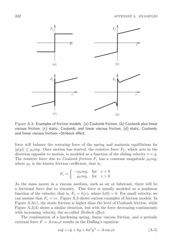
332 APPENDIX A. EXAMPLES
v v
(b)
v
(c)
v
(d)
(a)
Ff
Ff
Ff
Ff
Figure A.3: Examples of friction models. (a) Coulomb friction; (b) Coulomb plus linearviscous friction; (c) static, Coulomb, and linear viscous friction; (d) static, Coulomb,and linear viscous friction—Stribeck effect.
force will balance the restoring force of the spring and maintain equilibrium for|g(y)| ≤ μsmg. Once motion has started, the resistive force Ff , which acts in thedirection opposite to motion, is modeled as a function of the sliding velocity v = y.The resistive force due to Coulomb friction Fc has a constant magnitude μkmg,where μk is the kinetic friction coefficient, that is,
Fc ={ −μkmg, for v < 0
μkmg, for v > 0
As the mass moves in a viscous medium, such as air or lubricant, there will bea frictional force due to viscosity. This force is usually modeled as a nonlinearfunction of the velocity; that is, Fv = h(v), where h(0) = 0. For small velocity, wecan assume that Fv = cv. Figure A.3 shows various examples of friction models. InFigure A.3(c), the static friction is higher than the level of Coulomb friction, whileFigure A.3(d) shows a similar situation, but with the force decreasing continuouslywith increasing velocity, the so-called Stribeck effect.
The combination of a hardening spring, linear viscous friction, and a periodicexternal force F = A cos ωt results in the Duffing’s equation
my + cy + ky + ka2y3 = A cos ωt (A.5)
A.3. TUNNEL-DIODE CIRCUIT 333
which is a classical example in the study of periodic excitation of nonlinear systems.The combination of a linear spring, static friction, Coulomb friction, linear vis-
cous friction, and external force F results in
my + ky + cy + η(y, y) = F
where
η(y, y) =
⎧⎨⎩
μkmg sign(y), for |y| > 0−ky, for y = 0 and |y| ≤ μsmg/k−μsmg sign(y), for y = 0 and |y| > μsmg/k
The value of η(y, y) for y = 0 and |y| ≤ μsmg/k is obtained from the equilibriumcondition y = y = 0. With x1 = y, x2 = y, and u = F , the state model is
x1 = x2, x2 = [−kx1 − cx2 − η(x1, x2) + u]/m (A.6)
Let us note two features of this state model. First, with u = 0 it has an equilibriumset, rather than isolated equilibrium points. Second, the right-hand side is a discon-tinuous function of the state. The discontinuity is a consequence of the idealizationwe adopted in modeling friction. One would expect the transition from static tosliding friction to take place in a smooth way, not abruptly as our idealization sug-gests.1 The discontinuous idealization, however, allows us to carry out piecewiselinear analysis since in each of the regions {x2 > 0} and {x2 < 0}, we can use themodel
x1 = x2, x2 = [−kx1 − cx2 − μkmg sign(x2) + u]/m
to predict the behavior of the system via linear analysis.
A.3 Tunnel-Diode Circuit
Consider the tunnel-diode circuit shown in Figure A.4, where the diode is char-acterized by iR = h(vR) [25]. The energy-storing elements in this circuit are thecapacitor C and the inductor L. Assuming they are linear and time invariant, wecan model them by the equations
iC = CdvC
dtand vL = L
diLdt
where i and v are the current through and the voltage across an element, withthe subscript specifying the element. We take x1 = vC and x2 = iL as the statevariables and u = E as a constant input. To write the state equation for x1, we
1The smooth transition from static to sliding friction can be captured by dynamic frictionmodels; see, for example, [6] and [100].
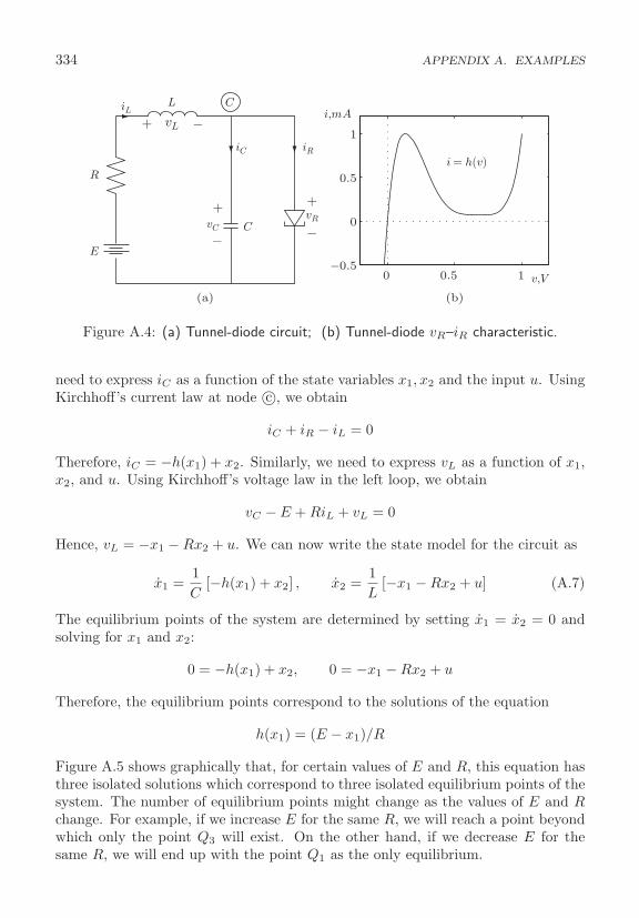
334 APPENDIX A. EXAMPLES
vCvR
iRiC
iL
R
E
L
C
+ +
vL+ −
− −
C
(a)
0 0.5 1−0.5
0
0.5
1
v,V
(b)
i,mA
i= h(v)
Figure A.4: (a) Tunnel-diode circuit; (b) Tunnel-diode vR–iR characteristic.
need to express iC as a function of the state variables x1, x2 and the input u. UsingKirchhoff’s current law at node c©, we obtain
iC + iR − iL = 0
Therefore, iC = −h(x1) + x2. Similarly, we need to express vL as a function of x1,x2, and u. Using Kirchhoff’s voltage law in the left loop, we obtain
vC − E + RiL + vL = 0
Hence, vL = −x1 − Rx2 + u. We can now write the state model for the circuit as
x1 =1C
[−h(x1) + x2] , x2 =1L
[−x1 − Rx2 + u] (A.7)
The equilibrium points of the system are determined by setting x1 = x2 = 0 andsolving for x1 and x2:
0 = −h(x1) + x2, 0 = −x1 − Rx2 + u
Therefore, the equilibrium points correspond to the solutions of the equation
h(x1) = (E − x1)/R
Figure A.5 shows graphically that, for certain values of E and R, this equation hasthree isolated solutions which correspond to three isolated equilibrium points of thesystem. The number of equilibrium points might change as the values of E and Rchange. For example, if we increase E for the same R, we will reach a point beyondwhich only the point Q3 will exist. On the other hand, if we decrease E for thesame R, we will end up with the point Q1 as the only equilibrium.
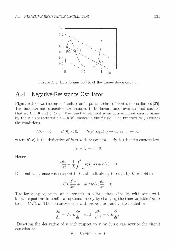
A.4. NEGATIVE-RESISTANCE OSCILLATOR 335
0 0.5 10
0.2
0.4
0.6
0.8
1
1.2
iR
Q1Q2
Q3
vR
Figure A.5: Equilibrium points of the tunnel-diode circuit.
A.4 Negative-Resistance Oscillator
Figure A.6 shows the basic circuit of an important class of electronic oscillators [25].The inductor and capacitor are assumed to be linear, time invariant and passive,that is, L > 0 and C > 0. The resistive element is an active circuit characterizedby the v–i characteristic i = h(v), shown in the figure. The function h(·) satisfiesthe conditions
h(0) = 0, h′(0) < 0, h(v) sign(v) → ∞ as |v| → ∞where h′(v) is the derivative of h(v) with respect to v. By Kirchhoff’s current law,
iC + iL + i = 0
Hence,
Cdv
dt+
1L
∫ t
−∞v(s) ds + h(v) = 0
Differentiating once with respect to t and multiplying through by L, we obtain
CLd2v
dt2+ v + Lh′(v)
dv
dt= 0
The foregoing equation can be written in a form that coincides with some well-known equations in nonlinear systems theory by changing the time variable from tto τ = t/
√CL. The derivatives of v with respect to t and τ are related by
dv
dτ=
√CL
dv
dtand
d2v
dτ2= CL
d2v
dt2
Denoting the derivative of v with respect to τ by v, we can rewrite the circuitequation as
v + εh′(v)v + v = 0

336 APPENDIX A. EXAMPLES
iLiC
C L
i
v
+
−
ResistiveElement
(a)
v
i= h(v)
(b)
Figure A.6: (a) Basic oscillator circuit; (b) Typical driving-point characteristic.
where ε =√
L/C. This equation is a special case of Lienard’s equation
v + f(v)v + g(v) = 0 (A.8)
When h(v) = −v + 13v3, the circuit equation takes the form
v − ε(1 − v2)v + v = 0 (A.9)
which is known as the Van der Pol equation. This equation, which was used byVan der Pol to study oscillations in vacuum tube circuits, is a fundamental examplein nonlinear oscillation theory. It possesses a periodic solution that attracts everyother solution except the zero solution at the unique equilibrium point v = v = 0.To write a state model for the circuit, let us take x1 = v and x2 = v to obtain
x1 = x2, x2 = −x1 − εh′(x1)x2 (A.10)
Alternatively, if we take the state variables as z1 = iL and z2 = vc, we obtain thestate model
z1 = z2/ε, z2 = ε[−z1 − h(z2)] (A.11)
The state models in the x and z coordinates look different, but they are equivalentrepresentations of the system. This equivalence can be seen by noting that thesemodels can be obtained from each other by a change of coordinates z = T (x). Sincewe have chosen both x and z in terms of physical variables, it is not hard to findthe map T . We have
x1 = v = z2
x2 =dv
dτ=
√CL
dv
dt=
√L
C[−iL − h(vC)] = ε[−z1 − h(z2)]
A.5. DC-TO-DC POWER CONVERTER 337
Thus,
z = T (x) =[ −h(x1) − x2/ε
x1
]and x = T−1(z) =
[z2
−εz1 − εh(z2)
]
If a current source with current u is connected in parallel with the circuit, we arriveat the forced equation
z1 = z2/ε, z2 = ε[−z1 − h(z2) + u] (A.12)
a special case of which is the forced van der Pol equation
z1 = z2/ε, z2 = ε[−z1 + z2 − 1
3z32 + u
](A.13)
A.5 DC-to-DC Power Converter
Figure A.7 shows the circuit of a DC-to-DC switched power converter, known as theboost converter, with ideal switch and passive linear components having capacitanceC, inductance L, and resistance R [128]. When the switch is in the s = 1 position,Kirchoff’s laws yield the equations
LdiLdt
= E, CdvC
dt= −vC
R
while in the s = 0 position the equations are
LdiLdt
= −vC + E, CdvC
dt= iL − vC
R
where iL is the current through the inductor, vC the voltage across the capacitor,and E the constant voltage of the voltage source. The foregoing equations can bewritten as
LdiLdt
= −(1 − s)vC + E, CdvC
dt= (1 − s)iL − vC
R(A.14)
where s is a discrete variable that takes the values 0 or 1. When the switchingvariable s(t) is a high-frequency square waveform of period T and duty ratio μ ∈(0, 1); that is,
s(t) =
⎧⎨⎩
1 for tk ≤ t < tk + μT
0 for tk + μT ≤ t < tk + T
averaging can be used to approximate (A.14) by the equations [11, Chapter 2]
LdiLdt
= −(1 − μ)vC + E, CdvC
dt= (1 − μ)iL − vC
R(A.15)
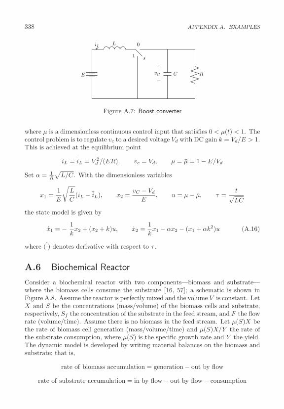
338 APPENDIX A. EXAMPLES
E
L
s1
0
C R
iL
vC
+
−
Figure A.7: Boost converter
where μ is a dimensionless continuous control input that satisfies 0 < μ(t) < 1. Thecontrol problem is to regulate vc to a desired voltage Vd with DC gain k = Vd/E > 1.This is achieved at the equilibrium point
iL = iL = V 2d /(ER), vc = Vd, μ = μ = 1 − E/Vd
Set α = 1R
√L/C. With the dimensionless variables
x1 =1E
√L
C(iL − iL), x2 =
vC − Vd
E, u = μ − μ, τ =
t√LC
the state model is given by
x1 = − 1k
x2 + (x2 + k)u, x2 =1k
x1 − αx2 − (x1 + αk2)u (A.16)
where ˙(·) denotes derivative with respect to τ .
A.6 Biochemical Reactor
Consider a biochemical reactor with two components—biomass and substrate—where the biomass cells consume the substrate [16, 57]; a schematic is shown inFigure A.8. Assume the reactor is perfectly mixed and the volume V is constant. LetX and S be the concentrations (mass/volume) of the biomass cells and substrate,respectively, Sf the concentration of the substrate in the feed stream, and F the flowrate (volume/time). Assume there is no biomass in the feed stream. Let μ(S)X bethe rate of biomass cell generation (mass/volume/time) and μ(S)X/Y the rate ofthe substrate consumption, where μ(S) is the specific growth rate and Y the yield.The dynamic model is developed by writing material balances on the biomass andsubstrate; that is,
rate of biomass accumulation = generation − out by flow
rate of substrate accumulation = in by flow − out by flow − consumption
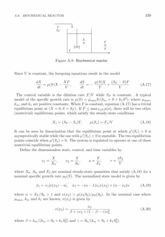
A.6. BIOCHEMICAL REACTOR 339
FXS
F
XS
V
SF
Figure A.8: Biochemical reactor.
Since V is constant, the foregoing equations result in the model
dX
dt= μ(S)X − XF
V,
dS
dt= − μ(S)X
Y+
(SF − S)FV
(A.17)
The control variable is the dilution rate F/V while SF is constant. A typicalmodel of the specific growth rate is μ(S) = μmaxS/(km + S + k1S
2), where μmax,km, and k1 are positive constants. When F is constant, equation (A.17) has a trivialequilibrium point at (X = 0, S = SF ). If F ≤ maxS≥0 μ(s), there will be two other(nontrivial) equilibrium points, which satisfy the steady-state conditions
Xs = (SF − Ss)Y, μ(Ss) = Fs/V (A.18)
It can be seen by linearization that the equilibrium point at which μ′(Ss) > 0 isasymptotically stable while the one with μ′(Ss) < 0 is unstable. The two equilibriumpoints coincide when μ′(Ss) = 0. The system is regulated to operate at one of thesenontrivial equilibrium points.
Define the dimensionless state, control, and time variables by
x1 =X
X0, x2 =
S
S0, u =
F
F0, τ =
tF0
V
where X0, S0, and F0 are nominal steady-state quantities that satisfy (A.18) for anominal specific growth rate μ0(S). The normalized state model is given by
x1 = x1[ν(x2) − u], x2 = −(α − 1)x1ν(x2) + (α − x2)u (A.19)
where α = SF /S0 > 1 and ν(x2) = μ(x2S0)/μ0(S0). In the nominal case whereμmax, km and k1 are known, ν(x2) is given by
ν(x2) =x2
β + γx2 + (1 − β − γ)x22
(A.20)
where β = km/(km + S0 + k1S20) and γ = S0/(km + S0 + k1S
20).
340 APPENDIX A. EXAMPLES
A.7 DC Motor
The equations of motion of the separately excited DC motor are given by [84]
Tadiadt
= −ia + va − φω (A.21)
Tfdφ
dt= −fe(φ) + vf (A.22)
Tmdω
dt= iaφ − f�(ω) − δ(t) (A.23)
where ia, va, φ, vf , and ω are normalized (dimensionless) armature current, ar-mature voltage, magnetic flux, field voltage, and speed, respectively, fe(φ) is theinverse normalized magnetization curve, f�(ω) + δ(t) is a normalized load torque,which consists of a speed-dependent term f�(ω) and a disturbance term δ(t), andTa, Tf and Tm are time constants.
The most common form to control a DC motor is the armature control methodwhere φ is constant and va is the control input. In this case, the model reduces toequations (A.21) and (A.23). Further simplification of this model results from thefact that Ta is typically much smaller than Tm. Neglecting the armature circuitdynamics by setting Ta = 0 yields ia = va − φω, which upon substitution in (A.23)results in the equation
Tmdω
dt= −φ2ω + φva − f�(ω) − δ(t)
Setting u = va/φ, η(ω) = f�(ω)/φ2, ϑ(t) = δ(t)/φ2, and defining the dimensionlesstime τ = tφ2/Tmo where Tmo is a nominal value of Tm, we obtain the normalizedmodel
ω = a[−ω + u − η(ω) − ϑ(t)] (A.24)
where a = Tmo/Tm, and ω = dω/dτ .In a field-controlled DC motor, vf is the control input while va is held constant
at va = Va. Taking x1 = ia, x2 = φ, and x3 = ω as the state variables, u = vf asthe control input, and τ = t/Tmo as dimensionless time, the state equation is givenby
x = f(x) + gu + hδ (A.25)
where x = dx/dτ , f = Dα, g = Dβ, h = Dγ,
D =
⎡⎣Tmo/Ta 0 0
0 Tmo/Tf 00 0 Tmo/Tm
⎤⎦ , α =
⎡⎣−x1 − x2x3 + Va
−fe(x2)x1x2 − f�(x3)
⎤⎦ , β =
⎡⎣0
10
⎤⎦ , γ =
⎡⎣0
01
⎤⎦
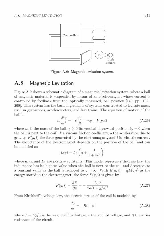
A.8. MAGNETIC LEVITATION 341
Lighsource
Controller
m
Figure A.9: Magnetic levitation system.
A.8 Magnetic Levitation
Figure A.9 shows a schematic diagram of a magnetic levitation system, where a ballof magnetic material is suspended by means of an electromagnet whose current iscontrolled by feedback from the, optically measured, ball position [149, pp. 192–200]. This system has the basic ingredients of systems constructed to levitate mass,used in gyroscopes, accelerometers, and fast trains. The equation of motion of theball is
md2y
dt2= −k
dy
dt+ mg + F (y, i) (A.26)
where m is the mass of the ball, y ≥ 0 its vertical downward position (y = 0 whenthe ball is next to the coil), k a viscous friction coefficient, g the acceleration due togravity, F (y, i) the force generated by the electromagnet, and i its electric current.The inductance of the electromagnet depends on the position of the ball and canbe modeled as
L(y) = L0
(α +
11 + y/a
)where a, α, and L0 are positive constants. This model represents the case that theinductance has its highest value when the ball is next to the coil and decreases toa constant value as the ball is removed to y = ∞. With E(y, i) = 1
2L(y)i2 as theenergy stored in the electromagnet, the force F (y, i) is given by
F (y, i) =∂E
∂y= − L0i
2
2a(1 + y/a)2(A.27)
From Kirchhoff’s voltage law, the electric circuit of the coil is modeled by
dφ
dt= −Ri + v (A.28)
where φ = L(y)i is the magnetic flux linkage, v the applied voltage, and R the seriesresistance of the circuit.
342 APPENDIX A. EXAMPLES
In what follows we develop two normalized models of the system: a two dimen-sional model in which the current i is treated as the control input and a three-dimensional model in which the voltage v is the control input. Treating the currentas the control input is valid when the time constant of the electric circuit is muchsmaller than the time constant of the mechanical motion, or when an inner high-gain feedback loop is closed around the circuit with feedback from the current. Incurrent control, we can substitute F from (A.27) into (A.26). However, the result-ing equation will depend nonlinearly on i. It is better to treat F as the controlinput and then solve (A.27) for i.
For the current-controlled system, we take the dimensionless time, state, andcontrol variables as
τ = λt, x1 =y
a, x2 =
1aλ
dy
dt, u =
F
mog
where λ2 = g/a and mo is a nominal mass. The state model is given by
x1 = x2, x2 = −bx2 + 1 + cu (A.29)
where xi denotes the derivative of xi with respect to τ , b = k/(λm), and c = mo/m.By definition, x1 ≥ 0 and u ≤ 0. In some of our investigations we will also considerthe constraint |F | ≤ Fmax, which will put a lower bound on u. For convenience, wewill take Fmax = 2mog so that −2 ≤ u ≤ 0.
For the voltage-controlled system, the current i is a state variable that satisfiesthe equation
L(y)di
dt= −Ri +
L0i
a(+y/a)2dy
dt+ v
which is obtained from (A.28) upon differentiating φ. With τ , x1, x2, b, and c asdefined earlier, let x3 = i/I and u = v/V , where the base current and voltage Iand V satisfy 8amog = L0I
2 and V = RI. The state model is given by
x1 = x2 (A.30)
x2 = −bx2 + 1 − 4cx23
(1 + x1)2(A.31)
x3 =1
T (x1)
[−x3 + u +
βx2x3
(1 + x1)2
](A.32)
where β = λL0/R and T (x1) = β[α + 1/(1 + x1)].
A.9 Electrostatic Microactuator
Figure A.10 shows a schematic diagram of of a parallel-plate electrostatic actuatordriven by a voltage source [120]. The equation of motion of the movable upperelectrode is
md2y
dt2+ b
dy
dt+ k(y − y0) = F

A.9. ELECTROSTATIC MICROACTUATOR 343
m
kb
R
y0vs va
is+
+
−− y
Figure A.10: Electrostatic microactuator
where m is the mass of the electrode, b the damping coefficient, k the elasticconstant, y the air gap, y0 the zero-voltage gap, and F the electrostatic force.To prevent contact between the electrodes, an insulating layer of thickness δy0 ismounted on the fixed electrode, with 0 < δ � 1. Consequently, y is constrained toδy0 ≤ y ≤ y0. The capacitance of the structure is C = εA/y, where A is the areaof the electrode and ε the permittivity of the gap. The electric energy stored in thecapacitance is E = 1
2Cv2a where va is the applied voltage, which is related to the
source voltage vs by the equation vs = va + Ris, in which is is the source currentand R its resistance. The force F is given by
F =∂E
∂y=
v2a
2∂C
∂y= − εAv2
a
2y2
Letting q = Cva be the electric charge on the capacitance, it follows that is = dq/dt.Therefore, the system is represented by the equations
md2y
dt2+ b
dy
dt+ k(y − y0) = − q2
2εA, R
dq
dt= vs − qy
εA
For a constant input vs = Vs, the equilibrium points satisfy the equation
Vs =q
C0− C0
2ky20
(q
C0
)3
where C0 = εA/y0 is the zero-voltage capacitance. By differentiation, it can beshown that the right-hand side of the foregoing equation increases monotonicallywith q until it reaches the maximum value Vp =
√8ky2
0/(27C0), then it decreasesmonotonically. Thus, for Vs < Vp, there are two equilibrium points, which mergeinto one point at Vs = Vp, while no equilibrium points exist for Vs > Vp. Open-loop control by applying a constant voltage Vs can stabilize the system only in alimited range of the air gap. Moreover, the transient response cannot be shaped as
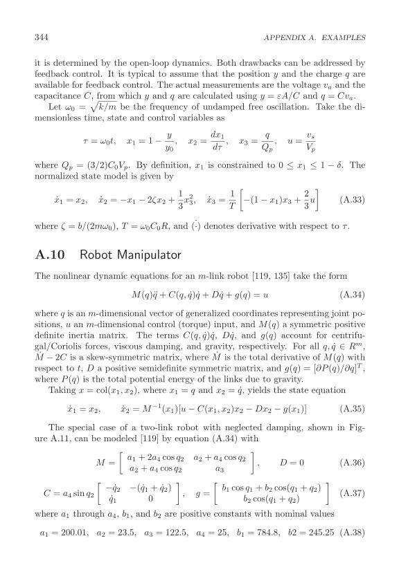
344 APPENDIX A. EXAMPLES
it is determined by the open-loop dynamics. Both drawbacks can be addressed byfeedback control. It is typical to assume that the position y and the charge q areavailable for feedback control. The actual measurements are the voltage va and thecapacitance C, from which y and q are calculated using y = εA/C and q = Cva.
Let ω0 =√
k/m be the frequency of undamped free oscillation. Take the di-mensionless time, state and control variables as
τ = ω0t, x1 = 1 − y
y0, x2 =
dx1
dτ, x3 =
q
Qp, u =
vs
Vp
where Qp = (3/2)C0Vp. By definition, x1 is constrained to 0 ≤ x1 ≤ 1 − δ. Thenormalized state model is given by
x1 = x2, x2 = −x1 − 2ζx2 +13x2
3, x3 =1T
[−(1 − x1)x3 +
23u
](A.33)
where ζ = b/(2mω0), T = ω0C0R, and ˙(·) denotes derivative with respect to τ .
A.10 Robot Manipulator
The nonlinear dynamic equations for an m-link robot [119, 135] take the form
M(q)q + C(q, q)q + Dq + g(q) = u (A.34)
where q is an m-dimensional vector of generalized coordinates representing joint po-sitions, u an m-dimensional control (torque) input, and M(q) a symmetric positivedefinite inertia matrix. The terms C(q, q)q, Dq, and g(q) account for centrifu-gal/Coriolis forces, viscous damping, and gravity, respectively. For all q, q ∈ Rm,M − 2C is a skew-symmetric matrix, where M is the total derivative of M(q) withrespect to t, D a positive semidefinite symmetric matrix, and g(q) = [∂P (q)/∂q]T ,where P (q) is the total potential energy of the links due to gravity.
Taking x = col(x1, x2), where x1 = q and x2 = q, yields the state equation
x1 = x2, x2 = M−1(x1)[u − C(x1, x2)x2 − Dx2 − g(x1)] (A.35)
The special case of a two-link robot with neglected damping, shown in Fig-ure A.11, can be modeled [119] by equation (A.34) with
M =[
a1 + 2a4 cos q2 a2 + a4 cos q2
a2 + a4 cos q2 a3
], D = 0 (A.36)
C = a4 sin q2
[ −q2 −(q1 + q2)q1 0
], g =
[b1 cos q1 + b2 cos(q1 + q2)
b2 cos(q1 + q2)
](A.37)
where a1 through a4, b1, and b2 are positive constants with nominal values
a1 = 200.01, a2 = 23.5, a3 = 122.5, a4 = 25, b1 = 784.8, b2 = 245.25 (A.38)
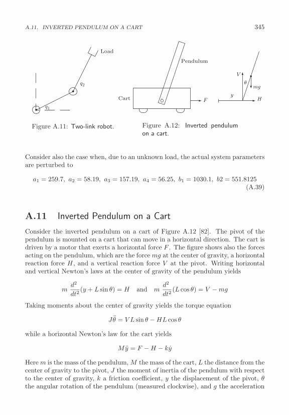
A.11. INVERTED PENDULUM ON A CART 345
q2
q1
Load
Figure A.11: Two-link robot.
FCarty
θmg
H
V
Pendulum
Figure A.12: Inverted pendulumon a cart.
Consider also the case when, due to an unknown load, the actual system parametersare perturbed to
a1 = 259.7, a2 = 58.19, a3 = 157.19, a4 = 56.25, b1 = 1030.1, b2 = 551.8125(A.39)
A.11 Inverted Pendulum on a Cart
Consider the inverted pendulum on a cart of Figure A.12 [82]. The pivot of thependulum is mounted on a cart that can move in a horizontal direction. The cart isdriven by a motor that exerts a horizontal force F . The figure shows also the forcesacting on the pendulum, which are the force mg at the center of gravity, a horizontalreaction force H, and a vertical reaction force V at the pivot. Writing horizontaland vertical Newton’s laws at the center of gravity of the pendulum yields
md2
dt2(y + L sin θ) = H and m
d2
dt2(L cos θ) = V − mg
Taking moments about the center of gravity yields the torque equation
Jθ = V L sin θ − HL cos θ
while a horizontal Newton’s law for the cart yields
My = F − H − ky
Here m is the mass of the pendulum, M the mass of the cart, L the distance from thecenter of gravity to the pivot, J the moment of inertia of the pendulum with respectto the center of gravity, k a friction coefficient, y the displacement of the pivot, θthe angular rotation of the pendulum (measured clockwise), and g the acceleration
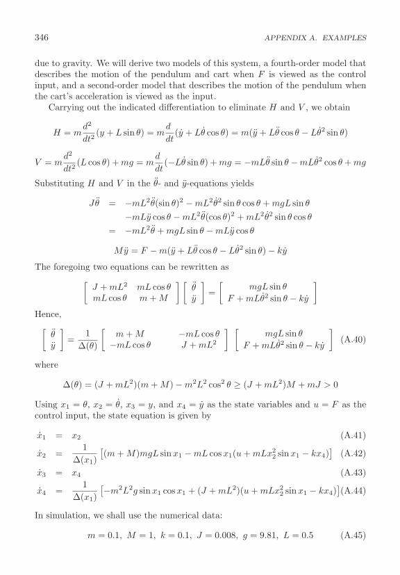
346 APPENDIX A. EXAMPLES
due to gravity. We will derive two models of this system, a fourth-order model thatdescribes the motion of the pendulum and cart when F is viewed as the controlinput, and a second-order model that describes the motion of the pendulum whenthe cart’s acceleration is viewed as the input.
Carrying out the indicated differentiation to eliminate H and V , we obtain
H = md2
dt2(y + L sin θ) = m
d
dt(y + Lθ cos θ) = m(y + Lθ cos θ − Lθ2 sin θ)
V = md2
dt2(L cos θ) + mg = m
d
dt(−Lθ sin θ) + mg = −mLθ sin θ −mLθ2 cos θ + mg
Substituting H and V in the θ- and y-equations yields
Jθ = −mL2θ(sin θ)2 − mL2θ2 sin θ cos θ + mgL sin θ
−mLy cos θ − mL2θ(cos θ)2 + mL2θ2 sin θ cos θ
= −mL2θ + mgL sin θ − mLy cos θ
My = F − m(y + Lθ cos θ − Lθ2 sin θ) − ky
The foregoing two equations can be rewritten as[J + mL2 mL cos θmL cos θ m + M
] [θy
]=[
mgL sin θ
F + mLθ2 sin θ − ky
]Hence,[
θy
]=
1Δ(θ)
[m + M −mL cos θ
−mL cos θ J + mL2
] [mgL sin θ
F + mLθ2 sin θ − ky
](A.40)
where
Δ(θ) = (J + mL2)(m + M) − m2L2 cos2 θ ≥ (J + mL2)M + mJ > 0
Using x1 = θ, x2 = θ, x3 = y, and x4 = y as the state variables and u = F as thecontrol input, the state equation is given by
x1 = x2 (A.41)
x2 =1
Δ(x1)[(m + M)mgL sin x1 − mL cos x1(u + mLx2
2 sin x1 − kx4)]
(A.42)
x3 = x4 (A.43)
x4 =1
Δ(x1)[−m2L2g sinx1 cos x1 + (J + mL2)(u + mLx2
2 sin x1 − kx4)](A.44)
In simulation, we shall use the numerical data:
m = 0.1, M = 1, k = 0.1, J = 0.008, g = 9.81, L = 0.5 (A.45)
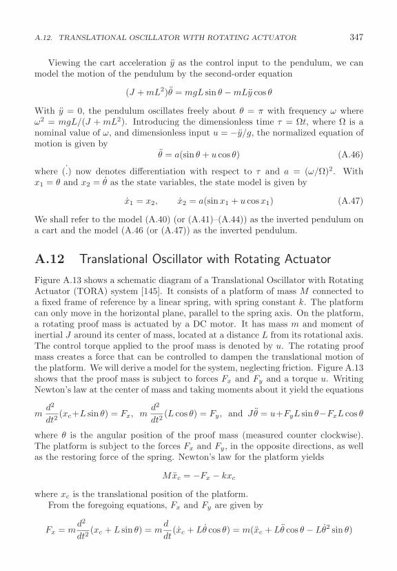
A.12. TRANSLATIONAL OSCILLATOR WITH ROTATING ACTUATOR 347
Viewing the cart acceleration y as the control input to the pendulum, we canmodel the motion of the pendulum by the second-order equation
(J + mL2)θ = mgL sin θ − mLy cos θ
With y = 0, the pendulum oscillates freely about θ = π with frequency ω whereω2 = mgL/(J + mL2). Introducing the dimensionless time τ = Ωt, where Ω is anominal value of ω, and dimensionless input u = −y/g, the normalized equation ofmotion is given by
θ = a(sin θ + u cos θ) (A.46)
where ˙(.) now denotes differentiation with respect to τ and a = (ω/Ω)2. Withx1 = θ and x2 = θ as the state variables, the state model is given by
x1 = x2, x2 = a(sin x1 + u cos x1) (A.47)
We shall refer to the model (A.40) (or (A.41)–(A.44)) as the inverted pendulum ona cart and the model (A.46 (or (A.47)) as the inverted pendulum.
A.12 Translational Oscillator with Rotating Actuator
Figure A.13 shows a schematic diagram of a Translational Oscillator with RotatingActuator (TORA) system [145]. It consists of a platform of mass M connected toa fixed frame of reference by a linear spring, with spring constant k. The platformcan only move in the horizontal plane, parallel to the spring axis. On the platform,a rotating proof mass is actuated by a DC motor. It has mass m and moment ofinertial J around its center of mass, located at a distance L from its rotational axis.The control torque applied to the proof mass is denoted by u. The rotating proofmass creates a force that can be controlled to dampen the translational motion ofthe platform. We will derive a model for the system, neglecting friction. Figure A.13shows that the proof mass is subject to forces Fx and Fy and a torque u. WritingNewton’s law at the center of mass and taking moments about it yield the equations
md2
dt2(xc+L sin θ) = Fx, m
d2
dt2(L cos θ) = Fy, and Jθ = u+FyL sin θ−FxL cos θ
where θ is the angular position of the proof mass (measured counter clockwise).The platform is subject to the forces Fx and Fy, in the opposite directions, as wellas the restoring force of the spring. Newton’s law for the platform yields
Mxc = −Fx − kxc
where xc is the translational position of the platform.From the foregoing equations, Fx and Fy are given by
Fx = md2
dt2(xc + L sin θ) = m
d
dt(xc + Lθ cos θ) = m(xc + Lθ cos θ − Lθ2 sin θ)
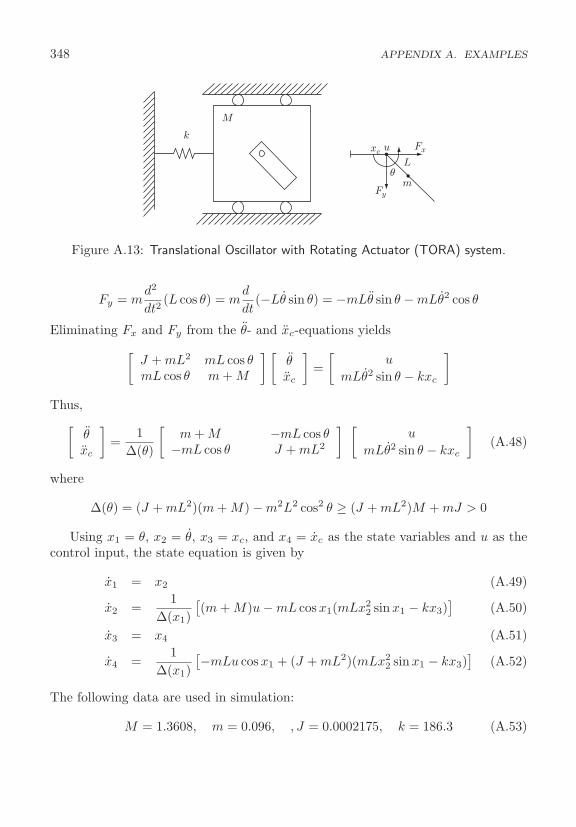
348 APPENDIX A. EXAMPLES
k
M
xcL
m
Fx
Fy
u
θ
Figure A.13: Translational Oscillator with Rotating Actuator (TORA) system.
Fy = md2
dt2(L cos θ) = m
d
dt(−Lθ sin θ) = −mLθ sin θ − mLθ2 cos θ
Eliminating Fx and Fy from the θ- and xc-equations yields[J + mL2 mL cos θmL cos θ m + M
] [θxc
]=[
u
mLθ2 sin θ − kxc
]
Thus,[θxc
]=
1Δ(θ)
[m + M −mL cos θ
−mL cos θ J + mL2
] [u
mLθ2 sin θ − kxc
](A.48)
where
Δ(θ) = (J + mL2)(m + M) − m2L2 cos2 θ ≥ (J + mL2)M + mJ > 0
Using x1 = θ, x2 = θ, x3 = xc, and x4 = xc as the state variables and u as thecontrol input, the state equation is given by
x1 = x2 (A.49)
x2 =1
Δ(x1)[(m + M)u − mL cos x1(mLx2
2 sin x1 − kx3)]
(A.50)
x3 = x4 (A.51)
x4 =1
Δ(x1)[−mLu cos x1 + (J + mL2)(mLx2
2 sin x1 − kx3)]
(A.52)
The following data are used in simulation:
M = 1.3608, m = 0.096, , J = 0.0002175, k = 186.3 (A.53)
Appendix B
Mathematical Review
Euclidean Space1
The set of all n-dimensional vectors x = col(x1, . . . , xn), where x1, . . . , xn are realnumbers, defines the n-dimensional Euclidean space denoted by Rn. The one-dimensional Euclidean space consists of all real numbers and is denoted by R.Vectors in Rn can be added by adding their corresponding components. They canbe multiplied by a scalar by multiplying each component by the scalar. The innerproduct of two vectors x and y is xT y =
∑ni=1 xiyi.
Vector and Matrix NormsThe norm ‖x‖ of a vector x is a real-valued function with the properties
• ‖x‖ ≥ 0 for all x ∈ Rn, with ‖x‖ = 0 if and only if x = 0.
• ‖x + y‖ ≤ ‖x‖ + ‖y‖, for all x, y ∈ Rn.
• ‖αx‖ = |α| ‖x‖, for all α ∈ R and x ∈ Rn.
The second property is the triangle inequality. We use the Euclidean (2-) norm,defined by
‖x‖ =(|x1|2 + · · · + |xn|2
)1/2=(xT x)1/2
An m× n matrix A of real elements defines a linear mapping y = Ax from Rn intoRm. The induced 2-norm of A is defined by
‖A‖ = max‖x‖=1
‖Ax‖ = max‖x‖≤1
‖Ax‖ =[λmax(AT A)
]1/2
where λmax(AT A) is the maximum eigenvalue of AT A. For real matrices A and Bof dimensions m × n and n × �, respectively, ‖AB‖ ≤ ‖A‖ ‖B‖.
1The mathematical review is patterned after similar reviews in [17] and [88]. For completecoverage of the reviewed topics, the reader may consult [3], [112], or [113].
349
350 APPENDIX B. MATHEMATICAL REVIEW
Quadratic FormsThe quadratic form of a real symmetric n × n matrix P is defined by
V (x) = xT Px =n∑
i=1
n∑j=1
pijxixj
It is positive semidefinite if V (x) ≥ 0 for all x and positive definite if V (x) > 0 forall x �= 0. It can be shown that V (x) is positive definite (positive semidefinite) ifand only if all the eigenvalues of P are positive (nonnegative), which is true if andonly if all the leading principal minors of P are positive (all principal minors of Pare nonnegative).2 If V (x) = xT Px is positive definite (positive semidefinite), wesay that the matrix P is positive definite (positive semidefinite) and write P > 0(P ≥ 0). The following relations of positive definite matrices are used in the text:
λmin(P )‖x‖2 ≤ xT Px ≤ λmax(P )‖x‖2 (B.1)
where λmin(P ) and λmax(P ) are the minimum and maximum eigenvalues of P ,respectively.
min‖x‖=r
xT Px = λmin(P )r2 (B.2)
For b ∈ Rn,3
min|bT x|=r
xT Px =r2
bT P−1b(B.3)
For a symmetric positive definite matrix P , the square root matrix P 1/2 is a sym-metric positive definite matrix such that P 1/2P 1/2 = P . For b ∈ Rn,
maxxT Px≤c
|bT x| = maxyT y≤1
‖√c bT P−1/2y‖ =√
c ‖bT P−1/2‖ (B.4)
where P−1/2 is the inverse of P 1/2.
Topological Concepts in Rn
Convergence of Sequences: A sequence of vectors x0, x1, . . ., xk, . . . in Rn,denoted by {xk}, converges to a limit vector x if
‖xk − x‖ → 0 as k → ∞
which is equivalent to saying that, given any ε > 0, there is an integer N such that
‖xk − x‖ < ε, ∀ k ≥ N
2This is a well-known fact in matrix theory. Its proof can be found in [15] or [44].3Following [89, Section 10.3], the Lagrangian associated with the constrained optimization
problem is L(x, λ) = xT Px + λ[(bT x)2 − r2]. The first-order necessary conditions are 2Px +2λ(bT x)b = 0 and (bT x)2 − r2 = 0. It can be verified that the solutions λ = −1/(bT P−1b) andx = ±rP−1b/(bT P−1b) yield the minimal value r2/(bT P−1b).
APPENDIX B. MATHEMATICAL REVIEW 351
The symbol “∀” reads “for all.” A vector x is an accumulation point of a sequence{xk} if there is a subsequence of {xk} that converges to x; that is, if there is aninfinite subset K of the nonnegative integers such that {xk}k∈K converges to x. Abounded sequence {xk} in Rn has at least one accumulation point in Rn. A sequenceof real numbers {rk} is increasing (monotonically increasing or nondecreasing) ifrk ≤ rk+1 ∀ k. If rk < rk+1, it is strictly increasing. Decreasing (monotonicallydecreasing or nonincreasing) and strictly decreasing sequences are defined similarlywith rk ≥ rk+1. An increasing sequence of real numbers that is bounded from aboveconverges to a real number. Similarly, a decreasing sequence of real numbers thatis bounded from below converges to a real number.
Sets: A subset S ⊂ Rn is open if, for every vector x ∈ S, one can find anε-neighborhood of x
N(x, ε) = {z ∈ Rn | ‖z − x‖ < ε}
such that N(x, ε) ⊂ S. A set S is closed if and only if its complement in Rn isopen. Equivalently, S is closed if and only if every convergent sequence {xk} withelements in S converges to a point in S. A set S is bounded if there is r > 0 suchthat ‖x‖ ≤ r for all x ∈ S. A set S is compact if it is closed and bounded. A pointp is a boundary point of a set S if every neighborhood of p contains at least onepoint of S and one point not belonging to S. The set of all boundary points of S,denoted by ∂S, is called the boundary of S. A closed set contains all its boundarypoints. An open set contains none of its boundary points. The interior of a set S isS − ∂S. An open set is equal to its interior. The closure of a set S, denoted by S,is the union of S and its boundary. A closed set is equal to its closure. An open setS is connected if every pair of points in S can be joined by an arc lying in S. A setS is called a region if it is the union of an open connected set with some, none, orall of its boundary points. If none of the boundary points are included, the regionis called an open region or domain. A set S is convex if, for every x, y ∈ S andevery real number θ, 0 < θ < 1, the point θx + (1 − θ)y ∈ S. If x ∈ X ⊂ Rn andy ∈ Y ⊂ Rm, we say that (x, y) belongs to the product set X × Y ⊂ Rn × Rm.
Continuous Functions: A function f mapping a set S1 into a set S2 is denotedby f : S1 → S2. A function f : Rn → Rm is continuous at a point x if f(xk) → f(x)whenever xk → x. Equivalently, f is continuous at x if, given ε > 0, there is δ > 0such that
‖x − y‖ < δ ⇒ ‖f(x) − f(y)‖ < ε
The symbol “⇒” reads “implies.” A function f is continuous on a set S if it iscontinuous at every point of S, and it is uniformly continuous on S if, given ε > 0there is δ > 0 (dependent only on ε) such that the inequality holds for all x, y ∈ S.Note that uniform continuity is defined on a set, while continuity is defined at apoint. For uniform continuity, the same constant δ works for all points in the set.Clearly, if f is uniformly continuous on a set S, then it is continuous on S. Theopposite statement is not true in general. However, if S is a compact set, then

352 APPENDIX B. MATHEMATICAL REVIEW
continuity and uniform continuity on S are equivalent. The function
(a1f1 + a2f2)(·) = a1f1(·) + a2f2(·)
is continuous for any two scalars a1 and a2 and any two continuous functions f1 andf2. If S1, S2, and S3 are any sets and f1 : S1 → S2 and f2 : S2 → S3 are functions,then the function f2 ◦ f1 : S1 → S3, defined by
(f2 ◦ f1)(·) = f2(f1(·))
is called the composition of f1 and f2. The composition of two continuous functionsis continuous. If S ⊂ Rn and f : S → Rm, then the set of f(x) such that x ∈ S iscalled the image of S under f and is denoted by f(S). If f is a continuous functiondefined on a compact set S, then f(S) is compact; hence, continuous functionson compact sets are bounded. Moreover, if f is real valued, that is, f : S → R,then there are points p and q in the compact set S such that f(x) ≤ f(p) andf(x) ≥ f(q) for all x ∈ S. If f is a continuous function defined on a connected setS, then f(S) is connected. A function f defined on a set S is one to one on S ifwhenever x, y ∈ S, and x �= y, then f(x) �= f(y). If f : S → Rm is a continuous,one-to-one function on a compact set S ⊂ Rn, then f has a continuous inversef−1 on f(S). The composition of f and f−1 is identity; that is, f−1(f(x)) = x.A function f : R → Rn is piecewise continuous on an interval J ⊂ R if for everybounded subinterval J0 ⊂ J , f is continuous for all x ∈ J0, except, possibly, at afinite number of points where f may have discontinuities. Moreover, at each pointof discontinuity x0, the right-side limit limh→0 f(x0 + h) and the left-side limitlimh→0 f(x0 − h) exist; that is, the function has a finite jump at x0.
Differentiable functions: A function f : R → R is differentiable at x if thelimit
f ′(x) = limh→0
f(x + h) − f(x)h
exists. The limit f ′(x) is called the derivative of f at x. A function f : Rn → Rm iscontinuously differentiable at a point x0 if the partial derivatives ∂fi/∂xj exist andare continuous at x0 for 1 ≤ i ≤ m, 1 ≤ j ≤ n. It is continuously differentiable ona set S if it is continuously differentiable at every point of S. It is of class C�, for� ≥ 1, on S if each fi has continuous partial derivatives up to order �. It is smoothif it is of class C∞. For a continuously differentiable function f : Rn → R, the rowvector ∂f/∂x is defined by
∂f
∂x=[
∂f
∂x1, . . . ,
∂f
∂xn
]
The gradient vector, denoted by ∇f(x), is
∇f(x) =[∂f
∂x
]T
APPENDIX B. MATHEMATICAL REVIEW 353
For a continuously differentiable function f : Rn → Rm, the Jacobian matrix[∂f/∂x] is an m×n matrix whose element in the ith row and jth column is ∂fi/∂xj .Suppose S ⊂ Rn is open, f maps S into Rm, f is continuously differentiable atx0 ∈ S, g maps an open set containing f(S) into Rk, and g is continuously differ-entiable at f(x0). Then the mapping h of S into Rk, defined by h(x) = g(f(x)), iscontinuously differentiable at x0 and its Jacobian matrix is given by the chain rule
∂h
∂x
∣∣∣∣x=x0
=∂g
∂f
∣∣∣∣f=f(x0)
∂f
∂x
∣∣∣∣x=x0
Mean Value and Implicit Function TheoremsIf x and y are two distinct points in Rn, then the line segment L(x, y) joining x andy is
L(x, y) = {z | z = θx + (1 − θ)y, 0 < θ < 1}Mean Value TheoremAssume that f : Rn → R is continuously differentiable at each point x of an
open set S ⊂ Rn. Let x and y be two points of S such that the line segmentL(x, y) ⊂ S. Then there is a point z of L(x, y) such that
f(y) − f(x) =∂f
∂x
∣∣∣∣x=z
(y − x) (B.5)
When f : Rn → Rn, a multidimensional version of the Mean Value Theorem isgiven by
f(y) − f(x) =∫ 1
0
∂f
∂x(x + σ(y − x)) dσ (y − x) (B.6)
which can be seen by setting J(x) = [∂f/∂x](x), and h(σ) = f(x + σ(y − x)) for0 ≤ σ ≤ 1. By the chain rule, h′(σ) = J(x + σ(y − x))(y − x). Using
f(y) − f(x) = h(1) − h(0) =∫ 1
0
h′(σ) dσ
we arrive at (B.6).Implicit Function TheoremAssume that f : Rn×Rm → Rn is continuously differentiable at each point (x, y)
of an open set S ⊂ Rn × Rm. Let (x0, y0) be a point in S for which f(x0, y0) = 0and for which the Jacobian matrix [∂f/∂x](x0, y0) is nonsingular. Then there existneighborhoods U ⊂ Rn of x0 and V ⊂ Rm of y0 such that for each y ∈ V theequation f(x, y) = 0 has a unique solution x ∈ U . Moreover, this solution can begiven as x = g(y), where g is continuously differentiable at y = y0.
The proofs of the mean-value and implicit-function theorems, as well as theother facts stated earlier in this appendix, can be found in any textbook on ad-vanced calculus or mathematical analysis.4
4See, for example, [3].
354 APPENDIX B. MATHEMATICAL REVIEW
Lemma B.1 (Gronwall–Bellman Inequality)5 Let λ : [a, b] → R be continuousand μ : [a, b] → R be continuous and nonnegative. If a continuous function y :[a, b] → R satisfies
y(t) ≤ λ(t) +∫ t
a
μ(s)y(s) ds
for a ≤ t ≤ b, then on the same interval
y(t) ≤ λ(t) +∫ t
a
λ(s)μ(s) exp[∫ t
s
μ(τ) dτ
]ds
In particular, if λ(t) ≡ λ is a constant, then
y(t) ≤ λ exp[∫ t
a
μ(τ) dτ
]
If, in addition, μ(t) ≡ μ ≥ 0 is a constant, then
y(t) ≤ λ exp[μ(t − a)]
�
Lemma B.2 (Comparison Lemma)6 Consider the scalar differential equation
u = f(t, u), u(t0) = u0
where f(t, u) is continuous in t and locally Lipschitz in u, for all t ≥ 0 and allu ∈ J ⊂ R. Let [t0, T ) (T could be infinity) be the maximal interval of existenceof the solution u(t), and suppose u(t) ∈ J for all t ∈ [t0, T ). Let v(t) be a con-tinuous function whose upper right-hand derivative D+v(t) satisfies the differentialinequality
D+v(t) ≤ f(t, v(t)), v(t0) ≤ u0
with v(t) ∈ J for all t ∈ [t0, T ). Then, v(t) ≤ u(t) for all t ∈ [t0, T ). �
5See [74, Lemma A.1] for the proof.6See [74, Lemma 3.4] for the proof. If v(t) is differentiable at t, then D+v(t) = v(t). If
|v(t + h) − v(t)| /h ≤ g(t, h), ∀ h ∈ (0, b], and limh→0+ g(t, h) = g0(t), then D+v(t) ≤ g0(t).

Appendix C
Composite LyapunovFunctions
The main challenge in Lyapunov theory is the search for a Lyapunov function. Auseful tool that helps this search is to represent the system as interconnection oflower-order components, find a Lyapunov function for each component, and usethem to form a composite Lyapunov function for the whole system. We illustratethis tool by examining cascade systems, interconnected systems with limited inter-connections [4, 93, 126] and singularly perturbed systems [76]. For convenience wepresent the idea for time-invariant systems and make use of quadratic-type Lya-punov functions, which were introduced in Section 4.2.
C.1 Cascade Systems
Consider the cascade connection
η = f1(η, ξ), ξ = f2(ξ) (C.1)
where f1 and f2 are locally Lipschitz and f1(0, 0) = 0, f2(0) = 0. In Lemma 4.6it is shown that if η = f1(η, ξ) is input-to-state stable and the origin of ξ = f2(ξ)is globally asymptotically stable, then the origin of (C.1) is globally asymptoticallystable. Here we show how to construct a Lyapunov function for the cascade connec-tion. For convenience, we assume that the origin of ξ = f2(ξ) is exponentially stableand there is a continuously differentiable Lyapunov function V2(ξ) that satisfies theinequalities
c1‖ξ‖2 ≤ V2(ξ) ≤ c2‖ξ‖2,∂V2
∂ξf2(ξ) ≤ −c3‖ξ‖2,
∥∥∥∥∂V2
∂ξ
∥∥∥∥ ≤ c4‖ξ‖ (C.2)
in some neighborhood of ξ = 0, where c1 to c4 are positive constants. Suppose theorigin of η = f1(η, 0) is asymptotically stable and there is a continuously differen-
355
356 APPENDIX C. COMPOSITE LYAPUNOV FUNCTIONS
tiable Lyapunov function V1(η) that satisfies the inequality
∂V1
∂ηf1(η, 0) ≤ −W1(η)
in some neighborhood of η = 0, where W1(η) is positive definite and continuous.Construct a composite Lyapunov function for the system (C.1) as
V (η, ξ) = bV1(η) +√
V2(ξ)
where b is a positive constant to be chosen. The derivative V is given by
V (η, ξ) = b∂V1
∂ηf1(η, ξ) +
12√
V2(ξ)∂V2
∂ξf2(ξ)
= b∂V1
∂ηf1(η, 0) + b
∂V1
∂η[f1(η, ξ) − f1(η, 0)] +
12√
V2(ξ)∂V2
∂ξf2(ξ)
On any bounded neighborhood of the origin, we can use continuous differentiabilityof V1 and the Lipschitz property of f1 to show that∥∥∥∥∂V1
∂η[f1(η, ξ) − f1(η, 0)]
∥∥∥∥ ≤ k‖ξ‖
for some positive constant k. Therefore
V (η, ξ) ≤ −bW1(η) + bk‖ξ‖ − c3
2√
c2‖ξ‖
Choosing b < c3/(2k√
c2) ensures that V is negative definite. The function V (η, ξ)is continuously differentiable everywhere around the origin, except on the manifoldξ = 0. Both V (η, ξ) and V (η, ξ) are defined and continuous around the origin. Itcan be easily seen that the statement of Theorem 3.3 is still valid and the origin of(C.1) is asymptotically stable.
The foregoing analysis is limited to a bounded neighborhood of the origin. Wecan remove this restriction and obtain a continuously differentiable composite Lya-punov function if V1(η) is a quadratic-type Lyapunov function. In particular, sup-pose V1(η) satisfies the inequalities
∂V1
∂ηf1(η, 0) ≤ −c φ2(η),
∥∥∥∥∂V1
∂η
∥∥∥∥ ≤ k φ(η) (C.3)
in some neighborhood of η = 0, where c and k are positive constants and φ is apositive definite continuous function, and take the composite Lyapunov function as
V (η, ξ) = bV1(η) + V2(ξ)

C.2. INTERCONNECTED SYSTEMS 357
in which b is a positive constant to be chosen. The derivative V satisfies
V (η, ξ) = b∂V1
∂ηf1(η, 0) + b
∂V1
∂η[f1(η, ξ) − f1(η, 0)] +
∂V2
∂ξf2(ξ)
≤ −bc φ2(η) + bkL φ(η)‖ξ‖ − c3‖ξ‖2
where L is a Lipschitz constant of f1 with respect to ξ. The right-hand-side of theforegoing inequality can be written as a quadratic form in (φ, ‖ξ‖), to obtain
V ≤ −[φ(η)‖ξ‖]T [
bc −bkL/2−bkL/2 c3
] [φ(η)‖ξ‖]
def= −[φ(η)‖ξ‖]T
Q
[φ(η)‖ξ‖]
The choice b < 4cc3/(kL)2 ensures that Q is positive definite, which shows that Vis negative definite; hence, the origin of (C.1) is asymptotically stable. If the as-sumptions hold globally and V1(η) is radially unbounded, the origin will be globallyasymptotically stable. If the origin of η = f1(η, 0) is exponentially stable and V1(η)satisfies inequalities similar to (C.2), then (C.3) is satisfied with φ(η) = ‖η‖. In thiscase the foregoing analysis shows that the origin of (C.1) is exponentially stable.
It is worthwhile to note that the same composite Lyapunov function can beconstructed for a system in the form
η = f1(η, ξ), ξ = f2(η, ξ)
if f2(η, 0) = 0 for all η and there is a Lyapunov function V2(ξ) that satisfies theinequalities
c1‖ξ‖2 ≤ V2(ξ) ≤ c2‖ξ‖2,∂V2
∂ξf2(η, ξ) ≤ −c3‖ξ‖2,
∥∥∥∥∂V2
∂ξ
∥∥∥∥ ≤ c4‖ξ‖
These inequalities show that the origin ξ = 0 is an exponentially stable equilibriumpoint of ξ = f2(η, ξ) uniformly in η.
C.2 Interconnected Systems
Consider the interconnected system
xi = fi(xi) + gi(x), i = 1, 2, . . . ,m (C.4)
where xi ∈ Rni , n1 + · · · + nm = n, x = col(x1, . . . , xm), and fi and gi are locallyLipschitz functions. Suppose fi(0) = 0 and gi(0) = 0 for all i so that the originx = 0 is an equilibrium point of (C.4). Ignoring the interconnection terms gi, thesystem decomposes into m isolated subsystems:
xi = fi(xi) (C.5)
358 APPENDIX C. COMPOSITE LYAPUNOV FUNCTIONS
with each one having an equilibrium point at its origin xi = 0. We start by searchingfor Lyapunov functions that establish asymptotic stability of the origin for eachisolated subsystem. Suppose this search has been successful and that, for eachsubsystem, we have a continuously differentiable Lyapunov function Vi(xi) whosederivative along the trajectories of the isolated subsystem (C.5) is negative definite.The function
V (x) =m∑
i=1
biVi(xi), bi > 0
is a composite Lyapunov function for the collection of the m isolated subsystemsfor all values of the positive constants bi. Viewing the interconnected system (C.4)as a perturbation of the isolated subsystems (C.5), it is reasonable to try V (x) as aLyapunov function candidate for (C.4). The derivative of V (x) along the trajectoriesof (C.4) is given by
V (x) =m∑
i=1
bi∂Vi
∂xifi(xi) +
m∑i=1
bi∂Vi
∂xigi(x)
The first term on the right-hand side is negative definite by virtue of the fact thatVi is a Lyapunov function for the ith isolated subsystem, but the second term is, ingeneral, indefinite. The situation is similar to our investigation of perturbed systemsin Section 4.2. Therefore, we may approach the problem by performing worst caseanalysis where the term [∂Vi/∂xi]gi is bounded by a nonnegative upper bound. Letus illustrate the idea by using quadratic-type Lyapunov functions. Suppose that,for i = 1, 2, . . . , m, Vi(xi) satisfies
∂Vi
∂xifi(xi) ≤ −ciφ
2i (xi),
∥∥∥∥∂Vi
∂xi
∥∥∥∥ ≤ kiφi(xi)
in some neighborhood of x = 0, for some positive constants ci and ki, and positivedefinite continuous functions φi. Furthermore, suppose that in the same neighbor-hood of x = 0, the interconnection terms gi(x) satisfy the bound
‖gi(x)‖ ≤m∑
j=1
γijφj(xj)
for some nonnegative constants γij . Then, the derivative of V (x) =∑m
i=1 biVi(xi)along the trajectories of the interconnected system (C.4) satisfies the inequality
V (x) ≤m∑
i=1
bi
⎡⎣−ciφ
2i (xi) +
m∑j=1
kiγijφi(xi)φj(xj)
⎤⎦
The right-hand side is a quadratic form in φ1, . . . , φm, which we rewrite as
V (x) ≤ − 12φT (DS + ST D)φ
C.3. SINGULARLY PERTURBED SYSTEMS 359
where φ = col(φ1, . . . , φm), D = diag(b1, . . . , bm), and S is an m×m matrix whoseelements are defined by
sij =
⎧⎨⎩
ci − kiγii, i = j
−kiγij , i �= j
If there is a positive diagonal matrix D such that DS + ST D > 0, then V (x) isnegative definite since φ(x) = 0 if and only if x = 0. Thus, a sufficient conditionfor asymptotic stability of the origin as an equilibrium point of the interconnectedsystem is the existence of a positive diagonal matrix D such that DS + ST D ispositive definite. This is the case if and only if S is an M -matrix;1 that is, the leadingprincipal minors of S are positive. The M -matrix condition can be interpretedas a requirement that the diagonal elements of S be “larger as a whole” thanthe off-diagonal elements. It can be seen that diagonally dominant matrices withnonpositive off-diagonal elements are M -matrices. The diagonal elements of S aremeasures of the “degree of stability” for the isolated subsystems in the sense that theconstant ci gives a lower bound on the rate of decrease of the Lyapunov function Vi
with respect to φ2i (xi). The off-diagonal elements of S represent the “strength of the
interconnections” in the sense that they give an upper bound on gi(x) with respectto φj(xj) for j = 1, . . . , m. Thus, the M -matrix condition says that if the degreesof stability for the isolated subsystems are larger as a whole than the strength ofthe interconnections, then the origin of the interconnected system is asymptoticallystable.
C.3 Singularly Perturbed Systems
Consider the singularly perturbed system
x = f(x, z), εz = g(x, z) (C.6)
where f and g are locally Lipschitz in a domain that contains the origin, ε is a smallpositive constant, f(0, 0) = 0, and g(0, 0) = 0. The system has a two-time-scalestructure because whenever |gi| ≥ k > 0, zi(t) moves faster in time than x(t). Areduced model that captures the slow motion of x can be obtained by setting ε = 0in the z-equation and solving for z in terms of x. Suppose z = h(x) is the uniquesolution of
0 = g(x, z)
in the domain of interest of x, h(x) is continuously differentiable with locally Lips-chitz partial derivatives, and h(0) = 0. Substitution of z = h(x) in the x-equationresults in the slow model
x = f(x, h(x)) (C.7)1See [93] for the proof of this fact.

360 APPENDIX C. COMPOSITE LYAPUNOV FUNCTIONS
The fast dynamics are captured by the z-equation when x is treated as a constantparameter. This can be seen by changing the time variable from t to τ = (t− t0)/εand setting ε = 0 in x(t0 + ετ), which freezes x at x(t0). The resulting fast modelis given by
dz
dτ= g(x, z) (C.8)
Our goal is to construct a composite Lyapunov function for the singularly perturbedsystem (C.6) as a weighted sum of Lyapunov functions for the slow and fast models.Because the fast model has an equilibrium point at z = h(x), it is more convenientto work in the (x, y)-coordinates, where
y = z − h(x)
This change of variables shifts the equilibrium point of the fast model to the origin.In the new coordinates, the singularly perturbed system is given by
x = f(x, y + h(x)), εy = g(x, y + h(x)) − ε∂h
∂xf(x, y + h(x)) (C.9)
Setting ε = 0 in the y-equation yields
0 = g(x, y + h(x))
whose unique solution is y = 0. Substitution of y = 0 in the x-equation resultsin the slow model (C.7). Changing the time variable in the y-equation from t toτ = (t − t0)/ε, and then setting ε = 0 on the right-hand side, results in the fastmodel
dy
dτ= g(x, y + h(x)) (C.10)
in which x is treated as a constant parameter. The slow model (C.7) has an equi-librium point at x = 0. Suppose this equilibrium point is asymptotically stableand there is a continuously differentiable Lyapunov function V1(x) that satisfies theinequality
∂V1
∂xf(x, h(x)) ≤ −a1φ
21(x) (C.11)
in some neighborhood of x = 0, where a1 is a positive constant and φ1 is a continuouspositive definite function. The fast model has an equilibrium point at y = 0.Suppose this equilibrium point is asymptotically stable and there is a continuouslydifferentiable Lyapunov function V2(x, y) such that
∂V2
∂yg(x, y + h(x)) ≤ −a2φ
22(y) (C.12)
in some neighborhood of (x = 0, y = 0), where a2 is a positive constant and φ2 isa continuous positive definite function. We allow V2 to depend on x because x is

C.3. SINGULARLY PERTURBED SYSTEMS 361
a parameter of the fast model and Lyapunov functions may, in general, depend onthe system’s parameters, but we require V2 to satisfy the inequalities
W1(y) ≤ V2(x, y) ≤ W2(y)
for some positive definite continuous functions W1 and W2. Now consider the com-posite Lyapunov function candidate
V (x, y) = bV1(x) + V2(x, y)
where b is a positive constant to be chosen. Calculating the derivative of V alongthe trajectories of (C.9), we obtain
V (x, y) = b∂V1
∂xf(x, y + h(x)) +
1ε
∂V2
∂yg(x, y + h(x))
−∂V2
∂y
∂h
∂xf(x, y + h(x)) +
∂V2
∂xf(x, y + h(x))
= b∂V1
∂xf(x, h(x)) +
1ε
∂V2
∂yg(x, y + h(x))
+b∂V1
∂x[f(x, y + h(x)) − f(x, h(x))] +
[∂V2
∂x− ∂V2
∂y
∂h
∂x
]f(x, y + h(x))
We have represented the derivative V as the sum of four terms. The first two termsare the derivatives of V1 and V2 along the trajectories of the slow and fast models.These two terms are negative definite in x and y, respectively, by inequalities (C.11)and (C.12). The other two terms represent the effect of the interconnection betweenthe slow and fast dynamics, which is neglected at ε = 0. Suppose that theseinterconnection terms satisfy the inequalities
∂V1
∂x[f(x, y + h(x)) − f(x, h(x))] ≤ k1φ1(x)φ2(y) (C.13)
[∂V2
∂x− ∂V2
∂y
∂h
∂x
]f(x, y + h(x)) ≤ k2φ1(x)φ2(y) + γφ2
2(y) (C.14)
for some nonnegative constants k1, k2, and γ. Using inequalities (C.11) to (C.14),we obtain
V (x, y) ≤ −ba1φ21(x) − 1
εa2φ
22(y) + bk1φ1(x)φ2(y) + k2φ1(x)φ2(y) + γφ2
2(y)
= −φT (x, y)Qφ(x, y)
where φ = col(φ1, φ2) and
Q =
⎡⎣ ba1 − 1
2bk1 − 12k2
− 12bk1 − 1
2k2 a2/ε − γ
⎤⎦
362 APPENDIX C. COMPOSITE LYAPUNOV FUNCTIONS
The right-hand side of the last inequality is negative definite when
ba1
(a2
ε− γ)
> 14 (bk1 + k2)2
Hence, for all
ε <4a1a2b
4a1bγ + (bk1 + k2)2
the origin of (C.6) is asymptotically stable.
Appendix D
Proofs
Proof of Lemma 9.5: Let V1(η) be a Lyapunov function for η = f0(η, 0) thatsatisfies
c1‖η‖2 ≤ V1(η) ≤ c2‖η‖2,∂V1
∂ηf0(η, 0) ≤ −c3‖η‖2,
∥∥∥∥∂V1
∂η
∥∥∥∥ ≤ c4‖η‖
in a domain Dη ⊂ Rn−ρ that contains the origin. The existence of V1(η) is guaran-teed by (the converse Lyapunov) Theorem 3.8. Let P = PT > 0 be the solution ofthe Lyapunov equation P (A − BK) + (A − BK)T P = −I. Let Dξ ⊂ Rρ be a do-main containing the origin such that Dη ×Dξ ⊂ Dz. As in Section C.1, a Lyapunovfunction for the nominal system (9.9) can be constructed as V (z) = bV1(η)+ ξT Pξ,with a sufficiently small b > 0. The derivative of V with respect to the perturbedsystem (9.11) is given by
V = b∂V1
∂ηf0(η, 0) + b
∂V1
∂η[f0(η, ξ) − f0(η, 0)]
+ ξT [P (A − BK) + (A − BK)T P ]ξ + 2ξT PBΔ(z)≤ −bc3‖η‖2 + bc4L‖η‖ ‖ξ‖ − ‖ξ‖2 + 2‖PB‖ ‖ξ‖ ‖Δ(z)‖
where L is a Lipschitz constant of f0 with respect to ξ over Dz. Using the bound‖Δ(z)‖ ≤ k‖z‖ + δ ≤ k‖η‖ + k‖ξ‖ + δ, we arrive at
V ≤ −bc3‖η‖2 + bc4L‖η‖ ‖ξ‖ − ‖ξ‖2 + 2k‖PB‖ ‖ξ‖2 + 2k‖PB‖ ‖ξ‖ ‖η‖+ 2δ‖PB‖ ‖ξ‖
= −[ ‖η‖
‖ξ‖]T [
bc3 −(k‖PB‖ + bc4L/2)−(k‖PB‖ + bc4L/2) 1 − 2k‖PB‖
] [ ‖η‖‖ξ‖
]+ 2δ‖PB‖ ‖ξ‖
def= −[ ‖η‖
‖ξ‖]T
(Q + kQ1)[ ‖η‖
‖ξ‖]
+ 2δ‖PB‖ ‖ξ‖
363

364 APPENDIX D. PROOFS
Choosing b < 4c3/(c4L)2 ensures that Q is positive definite. Then, there is k∗ > 0,dependent on b, such that for all k < k∗ the matrix Q + kQ1 is positive definite.Hence, if δ = 0 we can conclude that the origin of the perturbed system (9.11)is exponentially stable. When δ > 0 we continue the analysis to show ultimateboundedness. Let λm > 0 be the minimum eigenvalue of Q + kQ1. Then
V ≤ −λm‖z‖2 + 2δ‖PB‖ ‖z‖ ≤ −(1 − θ)λm‖z‖2, for ‖z‖ ≥ 2δ‖PB‖λmθ
for 0 < θ < 1. Application of Theorem 4.5 shows that there are positive constantsδ∗ and c such that ‖z(t)‖ will be ultimately bounded by δc if δ < δ∗. �
Proof of Theorem 12.5: Write the trajectory under state feedback as χr =(ηr, ξr) and the one under output feedback as χ = (η, ξ). As in the proof ofLemma 11.3, represent the dynamics of the observer using the scaled estimationerrors
ζi =ξi − ξi
ερ−i, 1 ≤ i ≤ ρ (D.1)
to obtainεζ = A0ζ + εB0Δ(t, χ, ξ)
where
A0 =
⎡⎢⎢⎢⎢⎢⎣
−α1 1 0 · · · 0−α2 0 1 · · · 0
.... . .
...−αρ−1 0 1−αρ 0 · · · · · · 0
⎤⎥⎥⎥⎥⎥⎦ , B0 =
⎡⎢⎢⎢⎢⎢⎣
00...01
⎤⎥⎥⎥⎥⎥⎦
and
Δ(t, χ, ξ) = a(η, ξ) − a0(ξ) + [b(η, ξ) − b0(ξ)]γs(ξ) + δ(t, η, ξ, γs(ξ))
The matrix A0 is Hurwitz by design. Because a0(ξ), b0(ξ), and γs(ξ) are globallybounded,
|Δ(t, χ, ξ)| ≤ L1, ∀ χ ∈ Ω, ξ ∈ Rρ, t ≥ 0 (D.2)
where throughout the proof Li, for i = 1, 2, . . ., denote positive constants inde-pendent of ε. Let P be the positive definite solution of the Lyapunov equationPA0 + AT
0 P = −I, W (ζ) = ζT Pζ, and Σ = {W (ζ) ≤ kε2}. The first step of theproof is to show that the constant k > 0 in the definition of Σ can be chosen suchthat, for sufficiently small ε, the set Ω×Σ is positively invariant; that is, χ(t0) ∈ Ωand ζ(t0) ∈ Σ imply that χ(t) ∈ Ω and ζ(t) ∈ Σ for all t ≥ t0. Using (D.2), it canbe shown that, for all χ ∈ Ω,
εW = −ζT ζ + 2εζT PB0Δ ≤ −‖ζ‖2 + 2εL1‖PB0‖ ‖ζ‖≤ − 1
2‖ζ‖2, ∀ ‖ζ‖ ≥ 4εL1‖PB0‖
APPENDIX D. PROOFS 365
Using the inequalities
λmin(P )‖ζ‖2 ≤ ζT Pζ ≤ λmax(P )‖ζ‖2
we arrive atεW ≤ −σW, ∀ W ≥ ε2W0 (D.3)
where σ = 1/(2λmax(P )) and W0 = λmax(P )(4L1‖PB0‖)2. Taking k = W0 showsthat ζ(t) cannot leave Σ because W is negative on its boundary. On the other hand,for ζ ∈ Σ, ‖ξ − ξ‖ ≤ L2ε. Using the Lipschitz property of β, ψ, and sat(·), it canbe shown that ‖γs(ξ) − γs(ξ)‖ ≤ L3ε/μ, where the μ factor appears because of thefunction sat(s/μ). Since γs(ξ) = γ(ξ) in Ω, we have
‖γ(ξ) − γs(ξ)‖ ≤ εL3
μ(D.4)
Inspection of equation (12.47) shows that the control u appears only in the s equa-tion. Using (D.4) and recalling the analysis of sliding mode control from Sec-tion 10.1, it can be shown that
ss ≤ b(η, ξ)[−β0|s| + εL3
μ|s|]
Taking ε ≤ μβ0/(2L3) yields
ss ≤ −(b0β0/2)|s|With this inequality, the analysis of Section 10.1 carries over to show that thetrajectory (η(t), ξ(t)) cannot leave Ω and enters Ωμ in finite time.
The second step of the proof is to show that for all χ(0) ∈ Ω0 and ξ(0) ∈ X, thetrajectory (χ(t), ζ(t)) enters Ω × Σ within a time interval [0, τ(ε)], where τ(ε) → 0as ε → 0. Notice that, due to the scaling (D.1), the initial condition ζ(0) could beof the order of 1/ερ−1. Because Ω0 is in the interior of Ω and the control γs(ξ) isglobally bounded, there is time T1 > 0, independent of ε, such that χ(t) ∈ Ω fort ∈ [0, T1]. During this time interval, (D.2) and consequently (D.3) hold. It followsfrom Theorem 4.5 that
W (t) ≤ max{
e−σt/εW (0), ε2W0
}≤ max
{e−σt/εL4
ε2(ρ−1), ε2W0
}
which shows that ζ(t) enters Σ within the time interval [0, τ(ε)] where
τ(ε) =ε
σln(
L4
W0ε2ρ
)
By l’Hopital’s rule it can be verified that limε→0 τ(ε) = 0. By choosing ε smallenough, we can ensure that τ(ε) < T1. Thus, the trajectory (χ(t), ζ(t)) is bounded
366 APPENDIX D. PROOFS
for all t ≥ 0 and enters the set Ωμ×Σ within finite time T . Because γs(ξ) is globallybounded and χ(0) = χr(0),
‖χ(t) − χr(t)‖ ≤ L5τ(ε) ∀ t ∈ [0, τ(ε)]
Over the interval [τ(ε), T ], the χ-equation under output feedback is O(ε) perturba-tion of the corresponding equation under state feedback. Therefore, (12.61) followsfrom continuous dependence of the solutions of differential equations on parame-ters.1 �
Proof of Theorem 12.6: Write the closed-loop system under state feedbackas
χ = f(χ, γ(ξ)) (D.5)
Inside Ωμ × Σ, the closed-loop system under output feedback is given by
χ = f(χ, γ(ξ − Dζ)), εζ = A0ζ + εB0Δ(t, χ, ξ − Dζ) (D.6)
where D is a diagonal matrix whose ith diagonal element is ερ−i and Δ(t, 0, 0) = 0.Because the origin of (D.5) is exponentially stable, by (the converse Lyapunov)Theorem 3.8 there is a Lyapunov function V (χ) that satisfies
c1‖χ‖2 ≤ V (χ) ≤ c2‖χ‖2,∂V
∂χf(χ, γ(ξ)) ≤ −c3‖χ‖2,
∥∥∥∥∂V
∂χ
∥∥∥∥ ≤ c4‖χ‖
in some neighborhood N of the origin, where c1 to c4 are positive constants. Takeμ small enough so that Ωμ ⊂ N . As in section C.3, we take Vc(χ, ζ) = V (χ)+W (ζ)as a Lyapunov function candidate for (D.6). It can be shown that
Vc ≤ −c3‖χ‖2 + c5‖χ‖ ‖ζ‖ − 1ε‖ζ‖2 + c6‖ζ‖2
for some positive constant c5 and c6. The foregoing inequality can be written as
Vc ≤ − 12c3(‖χ‖2 + ‖ζ‖2) − 1
2
[‖χ‖‖ζ‖]T [
c3 −c5
−c5 (2/ε − c3 − 2c6)
] [‖χ‖‖ζ‖]
The matrix of the quadratic form can be made positive definite by choosing ε smallenough. Then, Vc ≤ − 1
2c3(‖χ‖2 + ‖ζ‖2), which shows that the origin of (D.6) isexponentially stable and all trajectories in Ωμ ×Σ converge to the origin. Since alltrajectories with χ(0) ∈ Ω0 and ξ(0) ∈ X enter Ωμ × Σ, we conclude that Ω0 × Xis a subset of the region of attraction. �
Proof of Theorem 13.1: Using Assumption 13.6 we can show that there aretwo compact positively invariant sets Ω and Ωμ such that every trajectory starting
1See [74, Theorem 3.4].
APPENDIX D. PROOFS 367
in Ω enters Ωμ in finite time. The construction of Ω and Ωμ is done in three steps.We write the closed-loop system in the form
z = f0(z, e, r, w)ζ = Aζ + Bs
s = −b(η, ξ, w)β(η, ξ) sat(
s
μ
)+ Δ(η, ξ, r, w)
where ζ = col(e0, . . . , eρ−1), e = Aζ + Bs, and A is Hurwitz. For |s| ≥ μ, we have
ss ≤ b
[−β +
|Δ|b
]|s| ≤ b[−β + �]|s| ≤ −b0β0|s|
which shows that the set {|s| ≤ c}, with c > μ, is positively invariant. In the secondstep, we use the Lyapunov function V2(ζ) = ζT Pζ, where P is the solution of theLyapunov equation PA + AT P = −I, and the inequality
V2 ≤ −ζT ζ + 2‖ζ‖ ‖PB‖ |s|to show that the set {V2 ≤ c2ρ1} × {|s| ≤ c} is positively invariant, for ρ1 =(2||PB‖/θ)2λmax(P ), where 0 < θ < 1. Inside this set, we have ‖e‖ = ‖Aζ +Bs‖ ≤c‖A‖√ρ1/λmin(P ) + c
def= cρ2. Finally, we use the inequality
V1 ≤ −α3(‖z‖), ∀ ‖z‖ ≥ α4(cρ2)
to show that
Ω = {V1 ≤ α2(α4(cρ2))} × {V2 ≤ c2ρ1} × {|s| ≤ c}is positively invariant. Similarly, it can be shown that
Ωμ = {V1 ≤ α2(α4(μρ2))} × {V2 ≤ μ2ρ1} × {|s| ≤ μ}is positively invariant and every trajectory starting in Ω enters Ωμ in finite time.
Inside Ωμ, the system has an equilibrium point at (z = 0, ζ = ζ, s = s) whereζ = col(e0, 0, . . . , 0) and s = k0e0. Shifting the equilibrium point to the origin bythe change of variables ν = ζ − ζ and τ = s − s, the system takes the singularlyperturbed form
z = f0(z,Aν + Bτ, r, w)ν = Aν + Bτ
μτ = −b(η, ξ, w)β(η, ξ)τ + μΔ(z, ν, τ, r, w)
where Δ(0, 0, 0, r, w) = 0. Setting μ = 0 results in τ = 0 and yields the slow model
z = f0(z,Aν, r, w), ν = Aν
368 APPENDIX D. PROOFS
which is a cascade connection of z = f0(z,Aν, r, w) with ν = Aν. If z = 0 isan exponentially stable equilibrium point of z = f0(z, 0, r, w) and V0(z, r, w) is theconverse Lyapunov function provided by Theorem 3.8, we can construct a compositeLyapunov function αV0 + νT Pν with α > 0, as in Section C.1, to show that (z =0, ν = 0) is an exponentially stable equilibrium point of the slow model. Thenwe can construct a composite Lyapunov function V = αV0 + νT Pν + 1
2τ2, as inSection C.3 to show that, for sufficiently small μ, (z = 0, ν = 0, τ = 0) is anexponentially stable equilibrium point of the closed-loop system. It can be shownthat derivative of V satisfies the inequality
V ≤ −⎡⎣ ‖z‖
‖ν‖|τ |
⎤⎦T ⎡⎣ αk1 −αk2 −(αk3 + k4)
−αk2 1 −k5
−(αk3 + k4) −k5 (k6/μ) − k7
⎤⎦
︸ ︷︷ ︸Q
⎡⎣ ‖z‖
‖ν‖|τ |
⎤⎦
for some positive constants k1 to k7. The derivative V can be made negative definiteby choosing α < k1/k2
2 to make (q11q22 − q212) positive, and then choosing μ small
enough to make the determinant of Q positive. Hence, every trajectory in Ωμ
converges to the equilibrium point (z = 0, ν = 0, τ = 0) as t → ∞. Because e = 0at this point, we conclude that the error converges to zero. �
Bibliography
[1] B.D.O. Anderson and S. Vongpanitlerd. Network Analysis and Synthesis: AModern Systems Theory Approach. Prentice-Hall, Englewood Cliffs, NJ, 1973.
[2] P.J. Anstaklis and A.N. Michel. Linear Systems. McGraw-Hill, New York,1997.
[3] T.M. Apostol. Mathematical Analysis. Addison-Wesley, Reading, MA, 1957.
[4] M. Araki. Stability of large-scale nonlinear systems–quadratic-order theory ofcomposite-system method using M -matrices. IEEE Trans. Automat. Contr.,AC-23:129–141, 1978.
[5] M. Arcak and P. Kokotovic. Nonlinear observers: a circle criterion design androbustness analysis. Automatica, 37:1923–1930, 2001.
[6] B. Armstrong and C. Canudas de Wit. Friction modeling and compensation.In W. Levine, editor, The Control Handbook, pages 1369–1382. CRC Press,1996.
[7] R.B. Ash. Real Analysis and Probability. Academic Press, New York, 1972.
[8] A. Astolfi, D. Karagiannis, and R. Ortega. Nonlinear and Adaptive Controlwith Applications. Springer-Verlag, London, 2008.
[9] A.N. Atassi and H.K. Khalil. A separation principle for the stabilization ofa class of nonlinear systems. IEEE Trans. Automat. Contr., 44:1672–1687,1999.
[10] A. Bacciotti and L. Rosier. Lyapunov Functions and Stability in ControlTheory. Springer-Verlag, Berlin, 2005.
[11] S. Banerjee and G.C. Verghese, editors. Nonlinear Phenomena in PowerElectronics: Bifurcation, Chaos, Control, and Applications. IEEE Press, NewYork, 2001.
369
370 BIBLIOGRAPHY
[12] J.S. Baras, A. Bensoussan, and M.R. James. Dynamic observers as asymptoticlimits of recursive filters: speial cases. SIAM J. Applied Math, 48:1147–1158,1988.
[13] B.R. Barmish, M. Corless, and G. Leitmann. A new class of stabilizing con-trollers for uncertain dynamical systems. SIAM J. Control & Optimization,21:246–255, 1983.
[14] T. Basar and P. Bernhard. H∞-Optimal Control and Related Minimax DesignProblems. Birkhauser, Boston, second edition, 1995.
[15] R. Bellman. Introduction to Matrix Analysis. McGraw-Hill, New York, secondedition, 1970.
[16] B.W. Bequette. Process Dynamics: Modeling, Analysis, and Simulation.Prentice Hall, Upper Saddle River, NJ, 1998.
[17] D.P. Bertsekas. Dynamic Programming. Prentice-Hall, Englewood Cliffs, NJ,1987.
[18] F. Blanchini. Set invariance in control–a survey. Automatica, 35:1747–1767,1999.
[19] C.I. Byrnes and A. Isidori. Asymptotic stabilization of minimum phase non-linear systems. IEEE Trans. Automat. Contr., 36:1122–1137, 1991.
[20] C.I. Byrnes, A. Isidori, and J.C. Willems. Passivity, feedback equivalence, andthe global stabilization of minimum phase nonlinear systems. IEEE Trans.Automat. Contr., 36:1228–1240, 1991.
[21] F.M. Callier and C.A. Desoer. Multivariable Feedback Systems. Springer-Verlag, New York, 1982.
[22] C. T. Chen. Linear System Theory and Design. Holt, Rinehart and Winston,New York, 1984.
[23] G. Chesi. Domain of Attraction: Analysis and Control via SOS Programming.Springer-Verlag, London, 2011.
[24] S. Ching, Y. Eun, C. Gokcek, P.T. Kabamba, and S.M. Meerkov. QuasilinearControl: Performance Analysis and Design of Feedback Systems with Non-linear Sensors and Actuators. Cambridge University Press, Cambridge, UK,2011.
[25] L.O. Chua, C.A. Desoer, and E.S. Kuh. Linear and Nonlinear Circuits.McGraw-Hill, New York, 1987.
[26] L.O. Chua and Y. S. Tang. Nonlinear oscillation via volterra series. IEEETrans. Circuits Syst., CAS-29:150–168, 1982.
BIBLIOGRAPHY 371
[27] C.M. Close and D.K. Frederick. Modeling and Analysis of Dynamic Systems.Houghton Mifflin, Boston, second edition, 1993.
[28] M. Corless. Control of uncertain nonlinear systems. J. Dyn. Sys. Measurementand Control, 115:362–372, 1993.
[29] M. Corless and G. Leitmann. Continuous state feedback guaranteeing uniformultimate boundedness for uncertain dynamic systems. IEEE Trans. Automat.Contr., AC-26:1139–1144, 1981.
[30] M. Corless and R. Shorten. On the characterization of strict positive realnessfor general matrix transfer functions. IEEE Trans. Automat. Contr., 55:1899–1904, 2010.
[31] J-M. Coron. Control and Nonlinearity. American Mathematical Society, Prov-idence, RI, 2007.
[32] J-M. Coron, L. Praly, and A. Teel. Feedback stabilization of nonlinear sys-tems: sufficient conditions and Lyapunov and input–output techniques. InA. Isidori, editor, Trends in Control, pages 293–347. Springer-Verlag, NewYork, 1995.
[33] Z. Deng. Nonlinear and Adaptive Control. IET, London, 2013.
[34] C. Desoer and Y-T. Wang. Foundation of feedback theory for nonlinear dy-namical systems. IEEE Trans. Circuits Syst., 27:104–123, 1980.
[35] C.A. Desoer and M. Vidyasagar. Feedback Systems: Input–Output Properties.Academic Press, New York, 1975.
[36] A.B. Dixon, D.M. Dawson, and S. Nagarkatti. Nonlinear Control EngineeringSystems: A Lyapunov-Based Approach. Birkhauser, Boston, MA, 2003.
[37] J.C. Doyle, K. Glover, P.P. Khargonekar, and B.A. Francis. State-space so-lutions to standard H2 and H∞ control problems. IEEE Trans. Automat.Contr., 34:831–847, 1989.
[38] A.F. Filippov. Differential equations with discontinuous right-hand side.Amer. Math. Soc. Translations, 42:199–231, 1964.
[39] T.I. Fossen. Guidance and Control of Ocean Vehicles. John Wiley & Sons,New York, 1994.
[40] A.L. Fradkov, I.V. Miroshnik, and V.O. Nikiforov. Nonlinear and AdaptiveControl of Complex Systems. Springer, Netherlands, 1999.
[41] B.A. Francis. A course in H∞ control theory, volume 88 of Lect. Notes Contr.Inf Sci. Springer-Verlag, New York, 1987.
372 BIBLIOGRAPHY
[42] R.A. Freeman and P.V. Kokotovic. Optimal nonlinear controllers for feedbacklinearizable systems. In Proc. American Control Conf., pages 2722–2726,Seattle, WA, 1995.
[43] R.A. Freeman and P.V. Kokotovic. Robust Nonlinear Control Design: StateSpace and Lyapunov Techniques. Birkhauser, Boston, MA, 1996.
[44] F.R. Gantmacher. Theory of Matrices. Chelsea Publ., Bronx, NY, 1959.
[45] F.M. Gardner. Phaselock Techniques. Wiley-Interscience, New York, 1979.
[46] J-P. Gauthier and I. Kupka. Observability and Observers for Nonlinear Sys-tems. Cambridge University Press, Cambridge, UK, 2001.
[47] A. Gelb. Applied Optimal Estimation. MIT Press, Cambridge, MA, 1974.
[48] R. Genesio, M. Tartaglia, and A. Vicino. On the estimation of asymptoticstability regions: state of the rrt and new proposals. IEEE Trans. Automat.Contr., AC-30:747–755, 1985.
[49] W. Gerstner and W. Kistler. Spiking Neuron Models. Cambridge UniversityPress, Cambridge, UK, 2002.
[50] E. Gilbert and I. Kolmanovsky. Nonlinear tracking control in the presence ofstate and control constraints: a generalized reference governor. Automatica,38:2063–2073, 2002.
[51] G.H. Golub and C.F. Van Loan. Matrix Computations. The John HopkinsUniversity Press, Baltimore, 1983.
[52] J. Guckenheimer and P. Holmes. Nonlinear Oscillations, Dynamical Systems,and Bifurcations of Vector Fields. Springer-Verlag, New York, 1983.
[53] W.M. Haddad and V. Chellabonia. Nonlinear Dynamical Systems and Con-trol. Princeton University Press, Princeton, NJ, 2008.
[54] W. Hahn. Stability of Motion. Springer-Verlag, New York, 1967.
[55] J. Hale and H. Kocak. Dynamics and Bifurcations. Springer-Verlag, NewYork, 1991.
[56] J.K. Hale. Ordinary Differential Equations. Wiley-Interscience, New York,1969.
[57] K.M. Hangos, J. Bokor, and G. Szederkenyi. Analysis and Control of Nonlin-ear Process Systems. Springer, London, 2004.
[58] P. Hartman. Ordinary Differential Equations. Wiley, New York, 1964.
BIBLIOGRAPHY 373
[59] J. Hespanha. Linear Systems Theory. Princeton University Press, Princeton,NJ, 2009.
[60] D. Hill and P. Moylan. The stability of nonlinear dissipative systems. IEEETrans. Automat. Contr., AC-21:708–711, 1976.
[61] D.J. Hill and P.J. Moylan. Stability results for nonlinear feedback systems.Automatica, 13:377–382, 1977.
[62] M.W. Hirsch and S. Smale. Differential Equations, Dynamical Systems, andLinear Algebra. Academic Press, New York, 1974.
[63] J.C. Hsu and A.U. Meyer. Modern Control Principles and Applications.McGraw-Hill, New York, 1968.
[64] T. Hu and Z. Lin. Control Systems with Actuator Saturation: Analysis anddesign. Birkhauser, Boston, MA, 2001.
[65] T. Hu and Z. Lin. Composite quadratic Lyapunov functions for constrainedcontrol systems. IEEE Trans. Automat. Contr., 48:440–450, 2003.
[66] A. Isidori. Nonlinear Control Systems. Springer-Verlag, Berlin, third edition,1995.
[67] A. Isidori. Nonlinear Control Systems II. Springer-Verlag, London, 1999.
[68] A. Isidori and A. Astolfi. Disturbance attenuation and H∞ control via mea-surement feedback in nonlinear systems. IEEE Trans. Automat. Contr.,37:1283–1293, 1992.
[69] Z.P. Jiang, A.R. Teel, and L. Praly. Small gain theorem for ISS systems andapplications. Mathematics of Control, Signals, and Systems, 7:95–120, 1994.
[70] T. Kailath. Linear Systems. Prentice-Hall, Englewood Cliffs, NJ, 1980.
[71] L. Karafyllis and Z-P. Jiang. Stability and Stabilization of Nonlinear Systems.Springer, London, 2011.
[72] N. Kazantzis and C. Kravaris. Nonlinear observer design using Lyapunovauxiliary theorem. Syst. Contr. Lett., 34:241–247, 1998.
[73] H.K. Khalil. Universal integral controllers for minimum-phase nonlinear sys-tems. IEEE Trans. Automat. Contr., 45:490–494, 2000.
[74] H.K. Khalil. Nonlinear Systems. Prentice Hall, Upper Saddle River, NewJersey, third edition, 2002.
[75] P. Kokotovic and M. Arcak. Constructive nonlinear control: a historicalperspective. Automatica, 37:637–662, 2001.
374 BIBLIOGRAPHY
[76] P.V. Kokotovic, H.K. Khalil, and J. O’Reilly. Singular Perturbations Methodsin Control: Analysis and Design. SIAM, Philadelphia, PA, 1999.
[77] P.V. Kokotovic and R. Marino. On vanishing stability regions in nonlinearsystems with high-gain feedback. IEEE Trans. Automat. Contr., AC-31:967–970, 1986.
[78] N.N. Krasovskii. Stability of Motion. Stanford University Press, Stanford,1963.
[79] A.J. Krener. The convergence of the extended Kalman filter. In A. Rantzerand C.I. Byrnes, editors, Directions in Mathematical Systems Theory andOptimization, pages 173–182. Springer-Verlag, Berlin, 2003.
[80] M. Krstic and H. Deng. Stabilization of Uncertain Systems. Springer, London,1998.
[81] M. Krstic, I. Kanellakopoulos, and P. Kokotovic. Nonlinear and AdaptiveControl Design. Wiley-Interscience, New York, 1995.
[82] H. Kwakernaak and R. Sivan. Linear Optimal Control Systems. Wiley-Interscience, New York, 1972.
[83] J.P. LaSalle. An invariance principle in the theory of stability. In J.K. Hale andJ.P. LaSalle, editors, Differential Equations and Dynamical Systems, pages277–286. Academic Press, New York, 1967.
[84] W. Leonard. Control of Electrical Drives. Springer, Berlin, second edition,1996.
[85] A. Levant. Higher-order sliding modes, differentiation, and output-feedbackcontrol. Int. J. Contr., 76:924–941, 2003.
[86] Z. Lin and A. Saberi. Robust semi-global stabilization of minimum-phaseinput–output linearizable systems via partial state and output feedback. IEEETrans. Automat. Contr., 40:1029–1041, 1995.
[87] R. Lozano, B. Brogliato, O. Egeland, and B. Maschke. Dissipative SystemsAnalysis and Control: Theory and Applications. Springer, London, 2000.
[88] D.G. Luenberger. Optimization by Vector Space Methods. Wiley, New York,1969.
[89] D.G. Luenberger. Introduction to Linear and Nonlinear Programming.Addison-Wesley, Reading, MA, 1973.
[90] I.M.Y. Mareels and D.J. Hill. Monotone stability of nonlinear feedback sys-tems. J. Mathematical Systems, Estimation and Control, 2:275–291, 1992.
BIBLIOGRAPHY 375
[91] R. Marino and P. Tomei. Nonlinear Control Design: Geometric, Adaptive &Robust. Prentice-Hall, London, 1995.
[92] H.J. Marquez. Nonlinear Control Systems: Analysis and design. Wiley, Hobo-ken, FL, 2003.
[93] A.N. Michel and R.K. Miller. Qualitative Analysis of Large Scale DynamicalSystems. Academic Press, New York, 1977.
[94] A.N. Michel, N.R. Sarabudla, and R.K. Miller. Stability analysis of complexdynamical systems. Circuits Systems Signal Process, 1:171–202, 1982.
[95] R.K. Miller and A.N. Michel. Ordinary Differential Equations. AcademicPress, New York, 1982.
[96] J.B. Moore and B.D.O. Anderson. Applications of the multivariable Popovcriterion. Int.J. Control, 5:345–353, 1967.
[97] K.S. Narendra and J. Taylor. Frequency Domain Methods for Absolute Sta-bility. Academic Press, New York, 1973.
[98] H. Nijmeijer and A.J. van der Schaft. Nonlinear Dynamic Control Systems.Springer-Verlag, Berlin, 1990.
[99] E. Noldus and M. Loccufier. A new trajectory reversing method for theestimation of asymptotic stability regions. Int. J. Contr., 61:917–932, 1995.
[100] H. Olsson. Control Systems with Friction. PhD thesis, Lund Institute ofTechnology, Lund, Sweden, 1996.
[101] R. Ortega, A. Loria, P.J. Nicklasson, and H. Sira-Ramirez. Passivity-basedControl of Euler-Lagrange Systems. Springer, London, 1998.
[102] B.E. Paden and S.S. Sastry. A calculus for computing Filippov’s differentialinclusion with application to the variable structure control of robot manipu-lators. IEEE Trans. Circuits Syst.–I, CAS-34:73–82, 1987.
[103] M.A. Pai. Power System Stability Analysis by the Direct Method of Lyapunov.North-Holland, Amsterdam, 1981.
[104] T.S. Parker and L.O. Chua. Practical Numerical Algorithms for Chaotic Sys-tems. Springer-Verlag, New York, 1989.
[105] W.R. Perkins and J.B. Cruz. Engineering of Dynamic Systems. John Wiley,New York, 1969.
[106] W. Perruquetti and J-P. Barbot. Sliding Mode Control in Engineering. CRSPress, Boca Raton, FL, 2002.
376 BIBLIOGRAPHY
[107] Z. Qu. Robust control of nonlinear uncertain systems under generalizedmatching conditions. Automatica, 29:985–998, 1993.
[108] S. Raghavan and J.K. Hedrick. Observer design for a class of nonlinear sys-tems. Int. J. Contr., 59:515–528, 1994.
[109] R. Rajamani. Observers for Lipschitz nonlinear systems. IEEE Trans. Au-tomat. Contr., 43:397–401, 1998.
[110] K. Reif, F. Sonnemann, and R. Unbehauen. An EKF-based nonlinear observerwith a prescribed degree of stability. Automatica, 34:1119–1123, 1998.
[111] N. Rouche, P. Habets, and M. Laloy. Stability Theory by Lyapunov’s DirectMethod. Springer-Verlag, New York, 1977.
[112] H.L. Royden. Real Analysis. Macmillan, New York, 1963.
[113] W. Rudin. Principles of Mathematical Analysis. McGraw-Hill, New York,third edition, 1976.
[114] W.J. Rugh. Linear System Theory. Prentice-Hall, Upper Saddle River, NJ,second edition, 1996.
[115] A. Saberi, P.V. Kokotovic, and H.J. Sussmann. Global stabilization of par-tially linear composite systems. SIAM J. Control & Optimization, 28:1491–1503, 1990.
[116] M. Safonov. Stability and Robustness of Multivariable Feedback Systems. MITPress, Cambridge, MA, 1980.
[117] I.W. Sandberg. Global inverse function theorems. IEEE Trans. Circuits Syst.,CAS-27:998–1004, 1980.
[118] S. Sastry. Nonlinear Systems: Analysis, Stability and Control. Springer, NewYork, 1999.
[119] L. Sciavicco and B. Siciliano. Modeling and Control of Robot Manipulators.Springer-Velag, London, second edition, 2000.
[120] S.D. Senturia. Microsystem Design. Kluwer Academic, Norwell, MA, 2001.
[121] R. Sepulchre, M. Jankovic, and P. Kokotovic. Constructive Nonlinear Control.Springer, London, 1997.
[122] D. Shevitz and B. Paden. Lyapunov stability theory of nonsmooth systems.IEEE Trans. Automat. Contr., 39:1910–1914, 1994.
[123] H. Shim, J.H. seo, and A.R. Teel. Nonlinear observer design via passivationof error dynamics. Automatica, 39:885–892, 2003.

BIBLIOGRAPHY 377
[124] Y. Shtessel, C. Edwards, L. Fridman, and A. Levant. Sliding Mode Controland Observation. Birkhauser, Boston, MA, 2013.
[125] D.D. Siljak. Nonlinear Systems. Wiley, New York, 1969.
[126] D.D. Siljak. Large Scale Dynamic Systems: Stability and Structure. North-Holland, New York, 1978.
[127] D. Simon. Optimal State Estimation: Kalman, H-Infinity and Nonlinear Ap-proximation. Wiley Interscience, New York, 2006.
[128] H. Sira-Ramirez and M. Rios-Bolfvar. Sliding mode control of dc-to-dc powerconverters via extended linearization. IEEE Trans. Circuits Syst., 41:652–661,1994.
[129] J-J.E. Slotine and W. Li. Applied Nonlinear Control. Prentice Hall, Engle-wood Cliffs, NJ, 1991.
[130] E. Sontag and A. Teel. Changing supply functions in input/state stable sys-tems. IEEE Trans. Automat. Contr., 40:1476–1478, 1995.
[131] E.D. Sontag. Smooth stabilization implies coprime factorization. IEEE Trans.Automat. Contr., 34:435–443, 1989.
[132] E.D. Sontag. Mathematical Control Theory: Deterministic Finite Dimen-sional Systems. Springer, New York, second edition, 1998.
[133] E.D. Sontag. Input-to-state stability: Basic concepts and results. InA.A. Agrachev et.al., editor, Nonlinear and Optimal Control Theory. Springer-Verlag, Berlin, 2008.
[134] E.D. Sontag and Y. Wang. On characterizations of the input-to-state stabilityproperty. Syst. Contr. Lett., 24:351–359, 1995.
[135] M.W. Spong, S. Hutchinson, and M. Vidyasagar. Robot Modeling and Control.Wiley, Hoboken, New Jersey, 2005.
[136] S.H. Strogatz. Nonlinear Dynamics and Chaos. Addison Wesley, Reading,MA, 1994.
[137] H.J. Sussmann and P.V. Kokotovic. The peaking phenomenon and the globalstabilization of nonlinear systems. IEEE Trans. Automat. Contr., 36:424–440,1991.
[138] A.R. Teel. A nonlinear small-gain theorem for the analysis of control systemswith saturation. IEEE Trans. Automat. Contr., 41:1256–1270, 1996.
[139] A.R. Teel, T.T. Georgiou, L. Praly, and E. Sontag. Input-output stability. InW. Levine, editor, The Control Handbook. CRC Press, 1995.

378 BIBLIOGRAPHY
[140] U. Topcu, A.K. Packard, P. Seiler, and G.J. Balas. Robust region-of-attractionestimation. IEEE Trans. Automat. Contr., 55:137–142, 2010.
[141] J. Tsinias. Partial-state global stabilization for general triangular systems.Syst. Contr. Lett., 24:139–145, 1995.
[142] V. Utkin, J. Guldner, and J. Shi. Sliding Mode Control in ElectromechanicalSystems. CRS Press, Boca Raton, FL, second edition, 2009.
[143] A. van der Schaft. L2-Gain and Passivity Techniques in Nonlinear Control.Springer, London, 2000.
[144] M. Vidyasagar. Nonlinear Systems Analysis. SIAM, Philadelphia, PA, secondedition, 2002.
[145] C.-J. Wan, D.S. Bernstein, and V.T. Coppola. Global stabilization of theoscillating eccentric rotor. In Proc. IEEE Conf. on Decision and Control,pages 4024–4029, Orlando, FL, 1994.
[146] S. Wiggins. Introduction to Applied Nonlinear Dynamical Systems and Chaos.Springer-Verlag, New York, 1990.
[147] J.C. Willems. The Analysis of Feedback Systems. MIT Press, Cambridge,MA, 1971.
[148] J.L. Willems. The computation of finite stability regions by means of openLyapunov surfaces. Int.J. Control, 10:537–544, 1969.
[149] H.H. Woodson and J.R. Melcher. Electromechanical Dynamics, Part I: Dis-crete Systems. John Wiley, New York, 1968.
[150] F.F. Wu and C.A. Desoer. Global inverse function theorem. IEEE Trans.Circuit Theory, CT-19:199–201, 1972.
[151] V.A. Yakubovich, G.A. Leonov, and A.Kh. Gelig. Stability of Stationary Setsin Control Systems with Discontinuity. World Scientific, Singapore, 2004.
[152] T. Yoshizawa. Stability Theory By Liapunov’s Second Method. The Mathe-matical Society of Japan, Tokyo, 1966.
[153] K.D. Young, V.I. Utkin, and U. Ozguner. A control engineer’s guide to slidingmode control. IEEE Trans. Contr. Syst. Tech., 7:328–342, 1999.
[154] G. Zames. Feedback and optimal sensitivity: model reference transformations,multiplicative seminorms, and approximate inverses. IEEE Trans. Automat.Contr., AC-26:301–320, 1981.
[155] A. Zecevic and D.D. Siljak. Estimating the region of attraction for large scalesystems with uncertainties. Automatica, 46:445–451, 2010.

BIBLIOGRAPHY 379
[156] V.I. Zubov. Methods of A.M. Lyapunov and Their Application. Noordhoff,Groningen, The Netherlands, 1964.

Symbols1
≡ identically equal≈ approximately equal
def= defined as< (>) less (greater) than≤ (≥) less (greater) than or equal to� (�) much less (greater) than
∀ for all∈ belongs to⊂ subset of→ tends to⇒ implies⇔ equivalent to, if and only if∑
summation∏product
|a| the absolute value of a scalar a‖x‖ the norm of a vector x (349)‖A‖ the induced norm of a matrix A (349)max maximummin minimumsup supremum, the least upper boundinf infimum, the greatest lower boundRn the n-dimensional Euclidean space (349)Br the ball {x ∈ Rn | ‖x‖ ≤ r}M the closure of a set M
∂M the boundary of a set M(x, y) ∈ X × Y x ∈ X and y ∈ Y
dist(p,M) the distance from a point p toa set M (55)
f : S1 → S2 a function f mapping a set S1 intoa set S2 (351)
1The page where the symbol is defined is given in parentheses.
380
SYMBOLS 381
f2 ◦ f1 the composition of two functions (352)f−1(·) the inverse of a function f (352)
f ′(·) the first derivative of a real-valued function f (352)∇f the gradient vector (352)∂f∂x the Jacobian matrix (353)y the first derivative of y with respect to timey the second derivative of y with respect to time
y(i) the ith derivative of y with respect to timeLfh the Lie derivative of h with respect to
the vector field f (172)[f, g] the Lie bracket of the vector fields f and g (181)adk
fg [f, adk−1f g] (181)
diag[a1, . . . , an] a diagonal matrix with diagonalelements a1 to an
block diag[A1, . . . , An] a block diagonal matrix with diagonalblocks A1 to An
AT (xT ) the transpose of a matrix A ( a vector x)λmax(P ) (λmin(P )) the maximum (minimum) eigenvalue of
a symmetric matrix PP > 0 a positive definite matrix P (350)P ≥ 0 a positive semidefinite matrix P (350)
Re[z] or Re z the real part of a complex variable zIm[z] or Im z the imaginary part of a complex variable z
z or z∗ the conjugate of a complex variable zZ∗ the conjugate of a complex matrix Z
sat(·) the saturation function (238)Sat(·) the vector saturation function (243)sgn(·) the signum function (233)O(·) order of magnitude notation,
f(μ) = O(μ) ≡ |f(μ)| ≤ Kμ� designation of the end of theorems, lemmas,
and corollaries� designation of the end of examples� designation of the end of proofs
[xx] see reference number xx in the bibliography

Index
Asymptotic stability, 38global, 40global uniform, 77region of, 39uniform, 77
Autonomous system, 6
Backstepping, 211Barbashin–Krasovskii theorem, 57Basin, 40Biochemical reactor, 33, 194, 195, 228,
260, 338Boost converter, 119, 194, 195, 230, 280,
337Boundary layer, 238Boundedness, 85
Cascade systems, 355Causal mapping, 123Center, 20Chaos, 9Chattering, 236, 239Circle criterion, 157, 160
multivariable, 157Class K function, 76Class KL function, 76Comparison lemma, 354Control Lyapunov function, 223
global, 223robust, 223
Control saturation, 301Controller form, 179, 201Convergence, 350
Converse Lyapunov theorems, 68Corollary, see Corollary Index,Coulomb friction, 322
DC motor, 173, 179, 186, 195, 230, 327,340
DC-to-DC power converter, see boost con-verter
Decrescent function, 78Diffeomorphism, 7
global, 7local, 7
Distribution, 182involutive, 182
Domain, 351Domain of attraction, 40Duffing’s equation, 277Dynamic feedback, 197
Electrostatic microactuator, 194, 195, 196,229, 261, 278, 306, 326, 342,
Equilibrium points, 7continuum of, 7hyperbolic, 21isolated, 7
multiple, 8Existence and uniqueness, 5Exponential stability, 43, 77
global, 43, 77Extended Kalman Filter, 266
Fast model, 360Feedback linearization, 201
382

INDEX 383
Feedback passivation, 219, 285Feedforward, 309Finite escape time, 8Functions
composition of, 352continuous, 351
piecewise, 352uniformly, 351
continuously differentiable, 352differentiable, 352in C�, 352inverse of, 352one-to-one, 352smooth, 352
Gain function, 123Gain margin, 225Gradient vector, 352Gronwall–Bellman inequality, 354
H∞ control, 132H∞ norm, 133Hamilton–Jacobi–Bellman equation, 72Hamilton–Jacobi inequality, 135Hardening spring, 331Harmonic oscillator, 27, 279High-gain feedback, 248, 255, 257High-gain observer , 271, 288, 301, 323Holder’s inequalityHurwitz
matrix, 43transfer function, 112
Hydraulic systems, 12, 327
Implicit function theorem, 353Inner product, 349Input-to-state stability, 95, 98
regional, 98local, 98
Integral action, 318Interconnected systems, 357Invariance principle, 54
Invariant manifold, 242Invariant set, 55
positively, 55Inverted pendulum, 188, 195, 228, 261,
305, 347Inverted pendulum on a cart, 194, 228,
305, 345ISS, 95
Jacobian matrix, 7, 353Josephson junction, 11
Kalman–Yakubovich–Popov lemma, 114Krasovskii’s method, 71
L stability, 123connection with passivity, 134finite-gain, 123of state models, 127small-signal, 127
L2 gain, 132Lp space, 122LaSalle’s theorem, 56Lemma, see Lemma Index,Level surface, 49Lie bracket, 181Lie derivative, 172Lienard’s equation, 336Limit cycles, 8Linear growth bound, 80Linear time-invariant system, 40Linearization, 21, 43, 199, 263, 282Lipschitz
condition, 3globally, 3locally, 3
Loop transformation, 148Lossless system, 105, 109Lure’s problem, 156Lyapunov equation, 60Lyapunov function, 49
composite, 355
384 INDEX
cascade systems, 355interconnected systems, 357singularly perturbed systems, 359
control, 223energy, 51energy-like, 57Lure-type, 165quadratic, 50, 60, 157quadratic-type, 84, 356, 358ISS, 95
Lyapunov redesign, 251Lyapunov’s indirect method, 44Lyapunov’s stability theorem, 46
M-matrix, 359Magnetic levitation, 194, 195, 229, 245,
260, 294, 305, 325, 327, 341Mass–spring system, 12, 72, 119, 331Matched disturbance, 309Matched uncertainties, 231, 248Matching condition, 205Mean value theorem, 353Measurement noise, 273Min–max control, 252Minimum phase systems, 177, 296
Negative definite function, 49, 78Negative resistance oscillator, 7, 28, 335Negative semidefinite function, 49, 78Neuron (FitzHugh–Nagumo) model, 35Nodal sink, 18Nodal source, 19Nonautonomous system, 6Nonlinear phenomena, essentially, 8Nonlinearity
memoryless, 103saturation, 238sector, 106signum, 233
Norminduced matrix, 349vector, 349
Normal form, 171Nyquist criterion, 159
multivariable, 158Nyquist plot, 159
Observer-based control, 282, 286Observer form, 187Observers
global, 269high-gain, 271, 288local, 264nonlinear, 263with linear error dynamics, 270
Orbit, 15periodic (closed), 27
Output equation, 2Output feedback
regulation, 322stabilization, 281tracking, 322
Output feedback form, 193
Parseval’s theorem, 133Partial feedback linearization, 207Passive system, 105, 109
input strictly, 105, 109output strictly, 105, 109strictly, 109
Passivity, 103Passivity-based control, 217, 283Passivity theorems, 142PD controller, 220Peaking phenomenon, 210, 272, 289Pendulum 26, 45, 51, 73, 111, 140, 200,
233, 236, 255, 260, 279, 303,310, 313, 317, 321, 327, 329
Perturbationnonvanishing, 75structured, 82unstructured, 82vanishing, 75
Perturbed systems, 80

INDEX 385
Phase-locked loop, 12Phase plane, 15Phase portrait, 16PI controller, 321PID controller, 312Popov criterion, 164
multivariable, 165Popov plot, 167Positive definite function, 49, 78Positive definite matrix, 50, 350Positive limit point (set), 55Positive real lemma, 114Positive real transfer function, 112
strictly, 112Positive semidefinite function, 49, 78Positive semidefinite matrix, 50Practical stabilization, 231
global, 232local, 232regional, 232semiglobal, 232
Proper map, 7
Quadratic form, 50, 350
Radially unbounded function, 49, 78Reaching phase, 233Reference model, 308Region, 351Region of attraction, 39Regular form, 241Regulation, see robust regulationRelative degree
higher than one, 298linear systems, 112nonlinear systems, 172one, 296
Relaxation oscillation, 31Riccati equation, 267Robot manipulator, 11, 119, 180, 184,
188, 219, 230, 261, 278, 285,306, 326, 344
Robust regulationoutput feedback, 322state feedback, 318
Robust stabilizationoutput feedback, 296state feedback
Robustness, 91, 153, 154, 205Rotating rigid spacecraft, 119
Saddle, 19Saturation function, 238
vector, 243Scalar system, 39Sector condition (nonlinearity), 107Semitrailer-like vehicle, 195Separation principle, 288, 296Separatrix, 25Set, 351
boundary of, 351bounded, 351closed, 351closure of, 351compact, 351connected, 351interior of, 35open, 351
Set point, 314Signum function, 233Sliding mode control, 232, 233, 312, 319,
322, 323continuously implemented, 238
Sliding manifold, 233Sliding phase, 233Slow model, 359Small-gain theorem, 152Softening spring, 331Sontag’s formula, 223Spiral sink, 20Spiral source, 20Stability
absolute, 155, 156with a finite domain, 156
asymptotic, 38
386 INDEX
exponential, 43, 77input–output, 121input-to-state, 94L, 121matrix, 43of feedback systems, 141of equilibrium point, 37of linear system, 40of perturbed system, 80uniform, 77
Stabilization,global, 198local, 198practical, 231regional, 198robust, 231
via high-gain feedback, 257via Lyapunov redesign, 251via sliding mode control, 232
semiglobal, 198via backstepping, 211via feedback linearization, 201via linearization, 199via output feedback, 281via partial feedback linearization, 207via passivity-based control, 217via state feedback, 197
Stableequilibrium point, 38focus, 19limit cycle, 31node, 18structurally, 21
State equation, 2unforced, 2
State (–space) model, 2State plane, 15Static feedback, 197, 282Storage function, 109Stribeck effect, 332Strict feedback form, 214Strictly passive, 109Synchronous generator, 11
Time-invariant system, 6Time varying system, 6, 75TORA system, 194, 230, 261, 262, 306,
347Tracking, 307
output feedback, 322state feedback, 310robust, 312
Trajectory, 15Translational oscillator with rotating ac-
tuator, see TORATriangle inequality, 349Tunnel diode circuit, 24, 33, 119, 333
Ultimate boundedness, 85Underwater vehicle, 261, 328Unstable
equilibrium point, 38focus, 20limit cycle, 31node, 19
Van der Pol equation, 29, 173, 178, 196,228, 336
Variable gradient method, 52Variable structure control, see sliding mode
controlVector field, 15Vector field diagram, 15
Wien–bridge oscillator, 34, 278
Zero dynamics, 177Zero-state observable, 116
INDEX 387
Corollary Index1
6.1 (130) 8.1 (192)
Lemma Index
1.1 (5) 1.2 (5) 1.3 (5) 1.4 (7) 3.1 (56) 3.2 (61)4.1 (77) 4.2 (77) 4.3 (91) 4.4 (92) 4.5 (96) 4.6 (97)4.7 (98) 5.1 (112) 5.2 (114) 5.3 (114) 5.4 (114) 5.5 (115)5.6 (116) 6.1 (134) 9.1 (203) 9.2 (208) 9.3 (210) 9.4 (211)9.5 (211) 9.6 (224) 9.7 (226) 11.1 (265) 11.2 (267) 11.3 (176)12.1 (284) B.1 (354) B.2 (354)
Theorem Index
3.1 (41) 3.2 (44) 3.3 (47) 3.4 (56) 3.5 (57) 3.6 (58)3.7 (60) 3.8 (68) 3.9 (69) 4.1 (78) 4.2 (78) 4.3 (78)4.4 (87) 4.5 (89) 4.6 (95) 4.7 (98) 6.1 (127) 6.2 (131)6.3 (131) 6.4 (133) 6.5 (134) 6.6 (135) 6.7 (137) 6.8 (137)7.1 (143) 7.2 (143) 7.3 (146) 7.4 (147) 7.5 (149) 7.6 (150)7.7 (152) 7.8 (157) 7.9 (161) 7.10 (165) 8.1 (176) 8.2 (183)8.3 (191) 9.1 (218) 9.2 (222) 10.1 (245) 10.2 (247) 10.3 (253)10.4 (254) 12.1 (286) 12.2 (295) 12.3 (297) 12.4. (298) 12.5 (302)12.6 (302)
16.1(130) means Corollary 6.1 appears on page 130. The Lemma and Theorem Indexes arewritten similarly.