non-renewable resources, extraction technology, and ... · non-renewable resources, extraction...

NON-RENEWABLE RESOURCES,EXTRACTION TECHNOLOGY, AND

ENDOGENOUS GROWTH⇤

Martin Stuermer † Gregor Schwerho↵‡

July 16, 2016

Abstract

We develop a theory of innovation in non-renewable resource extraction andeconomic growth. Firms increase their economically extractable reserves of non-renewable resources through R&D investment in extraction technology and re-duce their reserves through extraction. Our model allows us to study the inter-action between geology and technological change, and its e↵ects on prices, totaloutput growth, and the resource intensity of the economy. The model accom-modates long-term trends in non-renewable resource markets – namely stableprices and exponentially increasing extraction – for which we present data ex-tending back to 1792. The paper suggests that over the long term, developmentof new extraction technologies balances the increasing demand for non-renewableresources. (JEL codes: O30, O41, Q30)

⇤ We thank Klaus Desmet, Martin Hellwig, Jurgen von Hagen, Anton Cheremukhin, Michael Sposi,Gordon Rausser, Thomas Covert, Maik Heinemann, Dirk Kruger, Pietro Peretto, Sjak Smulders,Lars Kunze, Florian Neukirchen, Gert Ponitzsch, Salim Rashid, Luc Rouge, Sandro Schmidt, andFriedrich-Wilhelm Wellmer for useful comments. We are highly grateful for comments of participantsat the NBER Summer Institute 2016, AEA annual meeting in Philadelphia, AERE summer meeting inBreckenridge, EAERE 2013 conference in Toulouse, SURED 2012 conference in Ascona, AWEEE 2012workshop in La Toja, SEEK 2012 conference in Mannheim, USAEE annual meeting in Pittsburgh,and SEA meeting in New Orleans, and at seminars at the U Chicago, U Cologne, U Bonn, MPI Bonn,and the Federal Reserve Bank of Dallas. We thank Mike Weiss for editing and Navi Dhaliwal, AchimGoheer and Ines Gorywoda for research assistance. All remaining errors are ours. An online-appendixis available from the authors upon request. An earlier version was published as a working paper withthe title “Non-renewable but inexhaustible: Resources in an endogenous growth model.” The viewsin this paper are those of the author and do not necessarily reflect the views of the Federal ReserveBank of Dallas or the Federal Reserve System.

†Federal Reserve Bank of Dallas, Research Department, Email: [email protected].‡Mercator Research Institute on Global Commons and Climate Change, Email: schwerho↵@mcc-

berlin.net

1 Introduction

In his seminal paper, Nordhaus (1974) estimates that the crustal abundance of non-

renewable resources is su�cient to continue consumption for hundreds of thousands

of years. He also emphasizes that prohibitively high extraction costs make a very

large share of mineral deposits not recoverable. Proven reserves – those non-renewable

resources that are economically recoverable with current technologies – are a far smaller

share.

However, innovation in extraction technology helps overcome scarcity by turning

mineral deposits into economically recoverable reserves (Nordhaus, 1974; Simon, 1981,

and others). There is empirical evidence for such technological change across a broad

variety of non-renewable resources (see, e.g., Managi et al., 2004; Mudd, 2007; Simpson,

1999).

In the literature on growth and natural resources, models rarely consider techno-

logical change in extraction. Scarcity is primarily overcome by technological change

involving the e�cient use of resources and substitution of capital for non-renewable

resources (see Groth, 2007; Aghion and Howitt, 1998). These models typically predict

decreased non-renewable resource extraction, and increasing prices in the long run,

which is not in line with empirical evidence of increasing production and non-increasing

prices (see Krautkraemer, 1998; Livernois, 2009; Von Hagen, 1989).

This paper develops a theory of technological change in non-renewable resource ex-

traction in an endogenous growth model. Modeling technological change in resource

extraction in a growth model is technically challenging because it adds a layer of dy-

2

namic optimization to the model. We boil down the investment and extraction problem

to a static problem, which makes our model both simple enough to solve and rich enough

to potentially connect to long-run data as a next step.

To our knowledge, our model is the first that allows the study of the interaction be-

tween technological change and geology, and its e↵ects on prices, total output growth,

and its use in the economy. Learning about these e↵ects is important for making pre-

dictions of long-run development of resource prices and for understanding the impact

of resource production on aggregate output. For example, distinguishing between in-

creasing and constant resource prices in the long run is key to the results of a number

of recent papers on climate economics (Acemoglu et al., 2012; Golosov et al., 2014;

Hassler and Sinn, 2012; van der Ploeg and Withagen, 2012).

We add an extractive sector to a standard endogenous growth model of expanding

varieties and directed technological change by Acemoglu (2002), such that aggregate

output is produced from non-renewable resources and intermediate goods.

Modeling the extractive sector has four components: First, we assume that there is a

continuum of deposits of declining grades. The quantity of the non-renewable resource

is distributed such that it increases exponentially as the ore grades of deposits decrease,

as a local approximation to Ahrens (1953, 1954) fundamental law of geochemistry.

Although we recognize that non-renewable resources are ultimately finite in supply,

we make the assumption that the underlying resource quantity goes to infinity for all

practical economic purposes as the grade of the deposits approaches zero. Without

innovation in extraction technology, the extraction cost is assumed to be infinitely

high.

3

Second, we build on Nordhaus’ (1974) idea that reserves are akin to working capital

or inventory of economically extractable resources. Firms can invest in grade specific

extraction technology to subsequently convert deposits of lower grades into economi-

cally extractable reserves. We assume that R&D investment exhibits decreasing returns

in making deposits of lower grades extractable, as historical evidence suggests. Once

converted into a reserve, the firm that developed the technology can extract the re-

source at a fixed operational cost.

Third, new technology di↵uses to all other firms. As each new technology is specific

to a deposit of a certain grade, it cannot be used to extract resources from deposits of

lower grades. However, all firms can build on existing technology when they invest in

developing new technology for deposits of lower grades. The idea is that firms can, for

example, use the shovel invented by another firm but have a cost to train employees to

use it for a specific deposit of lower grade. As technology di↵uses, firms only maximize

current profits in their R&D investment decisions in equilibrium.

Finally, the non-renewable resource is a homogeneous good. Despite a fully com-

petitive resource market in the long run, firms invest in extractive technology because

it is grade specific. Most similar to this understanding of innovation is Desmet and

Rossi-Hansberg (2014). We abstract from other possible features like uncertainty about

deposits, negative externalities from resource extraction, recycling, and short-run price

fluctuations.

Our model accommodates historical trends in the prices and production of major

non-renewable resources, as well as world real GDP for which we present data extend-

ing back to 1792. It implies a constant resource price equal to marginal cost over

4

the long run. Extraction firms face constant R&D costs in converting one unit of the

resource into a new reserve. This is due to the o↵setting interaction between techno-

logical change and geology: (i) new extraction technology exhibits decreasing returns

in making deposits of lower grades extractable; (ii) the resource quantity is geologically

distributed such that it increases exponentially as the grade of its deposits decreases.

The resource price depends negatively on the average crustal concentration of the

resource. For example, our model predicts that iron ore prices are on average lower

than copper prices, because iron is more abundant (5 percent of crustal mass) than

copper (0.007 percent). The price is also negatively a↵ected by the average e↵ect of

technology in terms of making lower grade deposits extractable. For example, the

average e↵ect might be larger for deposits that can be extracted in open pit mines (e.g.

coal) than for deposits requiring underground operations (e.g. crude oil). This implies

that coal prices are lower than crude oil price in the long term.

The resource intensity of the economy, defined as the resource quantity used to

produce one unit of aggregate output, is positively a↵ected by the average geologi-

cal abundance and the average e↵ect of extraction technology, while the elasticity of

substitution has a strong negative e↵ect. If the resource and the intermediate good

are complements, the resource intensity of the economy is relatively high, while it is

significantly lower in the case of the two being substitutes. As the resource intensity is

constant in equilibrium, firms extract the non-renewable resource at the same rate as

aggregate output.

Aggregate output growth is constant on the balanced growth path. Our model

predicts that a higher abundance of a particular resource or a higher average e↵ect of

5

extractive technology in terms of lower grades positively impact aggregate growth in

the long run.

The extractive sector features only constant returns to scale. In contrast to the

intermediate goods sector, where firms can make use of the entire stock of technology

for production, firms in the extractive sector can only use the flow of new technology

to convert deposits of lower grades into new reserves. Earlier developed technologies

are grade specific and the related deposits are exhausted. The stock of extraction tech-

nology therefore grows proportionally to output, while technology in the intermediate

goods sectors increases at the same rate as aggregate output.

The paper contributes to a literature that mostly builds on the seminal Hotelling

(1931) optimal depletion model. Heal (1976) introduces a non-renewable resource,

which is inexhaustible, but extractable at di↵erent grades and costs. Extraction costs

increase with cumulative extraction, but then remain constant when a “backstop tech-

nology” (Heal, 1976, p. 371) is reached. Slade (1982) adds exogenous technological

change in extraction technology to the Hotelling (1931) model and predicts a U-shaped

relative price curve. Cynthia-Lin and Wagner (2007) use a similar model with an in-

exhaustible non-renewable resource and exogenous technological change. They obtain

a constant relative price with increasing extraction.

There are three papers, to our knowledge, that like ours include technological

change in the extraction of a non-renewable resource in an endogenous growth model.

Fourgeaud et al. (1982) focuses on explaining sudden fluctuations in the development

of non-renewable resource prices by allowing the resource stock to grow in a stepwise

manner through technological change. Tahvonen and Salo (2001) model the transition

6

from a non-renewable energy resource to a renewable energy resource. Their model

follows a learning-by-doing approach as technological change is linearly related to the

level of extraction and the level of productive capital. It explains decreasing prices and

the increasing use of a non-renewable energy resource over a particular time period

before prices increase in the long term. Hart (2012) models resource extraction and

demand in a growth model with directed technological change. The key element in

his model is the depth of the resource. After a temporary “frontier phase” with a con-

stant resource price and consumption rising at a rate only close to aggregate output,

the economy needs to extract resources from greater depths. Subsequently, a long-run

balanced growth path is reached with constant resource consumption and prices that

rise in line with wages.

In Section 2, we document stylized facts on the long-term development of non-

renewable resource prices, production, and world real GDP. We also provide evidence

for the major assumptions of our model regarding geology and technological change.

Section 3 presents the setup of the growth model and its extractive sector. In section

4, we present and discuss the model’s theoretical implications. In Section 5 we draw

conclusions.

7

2 Stylized facts

2.1 Prices, Resource Production, and Aggregate Output over

the Long Term

Annual data for major non-renewable resource markets going back to 1792 indicate

that real prices are roughly trend-less and that worldwide primary production as well

as world real GDP grow roughly at a constant rate.

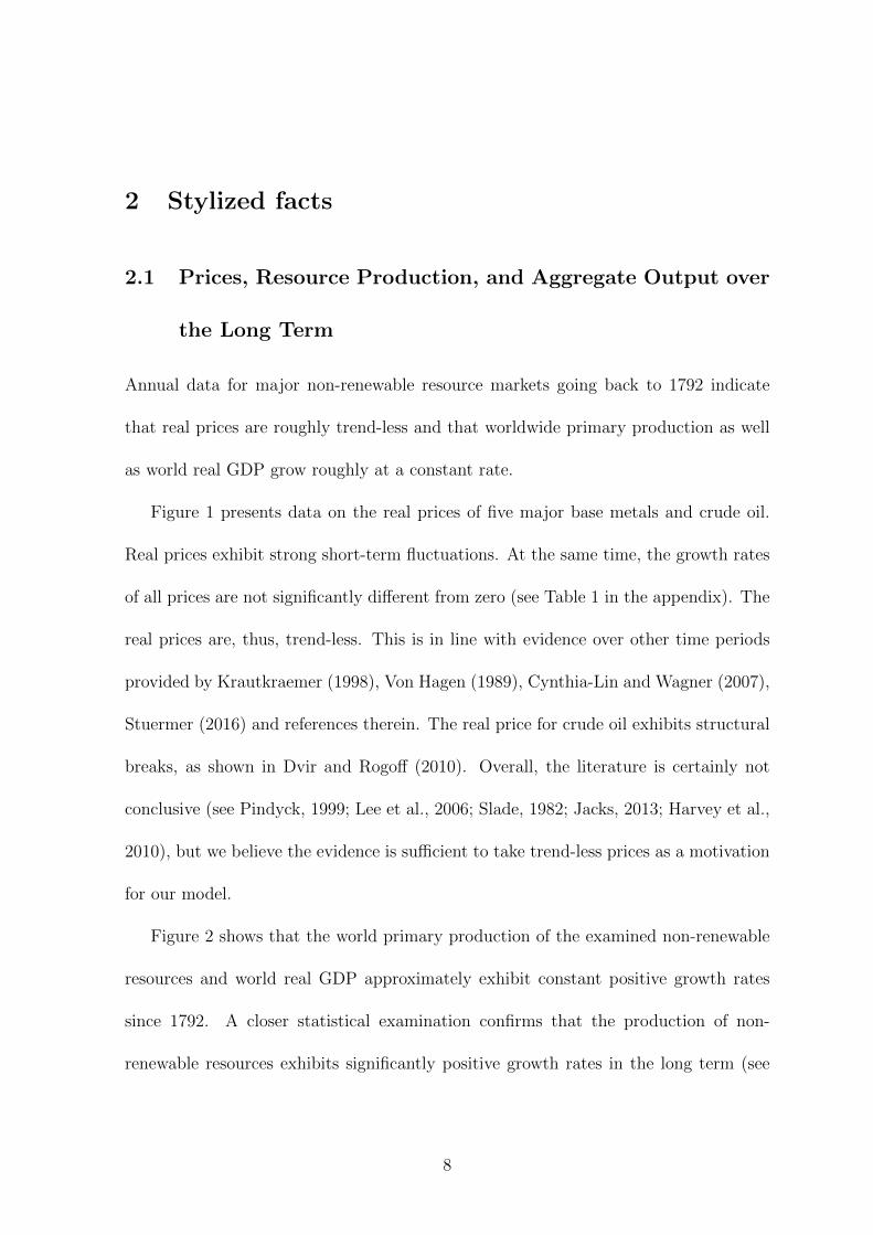
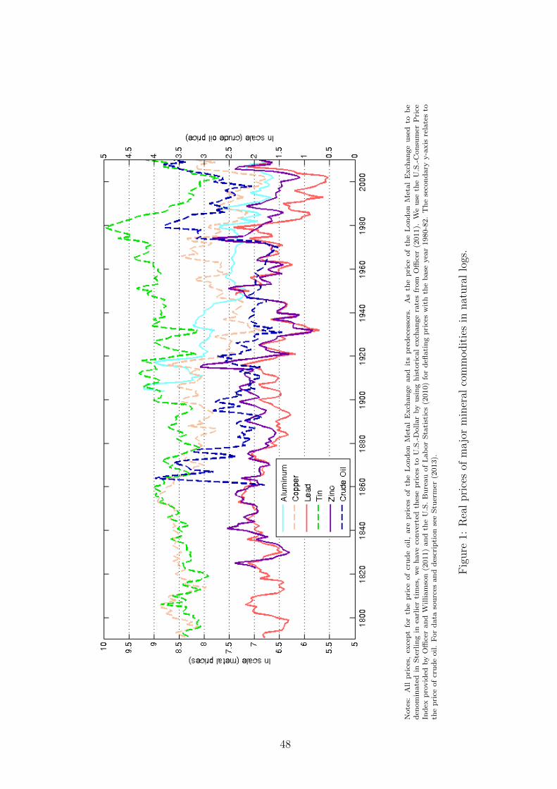
Figure 1 presents data on the real prices of five major base metals and crude oil.

Real prices exhibit strong short-term fluctuations. At the same time, the growth rates

of all prices are not significantly di↵erent from zero (see Table 1 in the appendix). The

real prices are, thus, trend-less. This is in line with evidence over other time periods

provided by Krautkraemer (1998), Von Hagen (1989), Cynthia-Lin and Wagner (2007),

Stuermer (2016) and references therein. The real price for crude oil exhibits structural

breaks, as shown in Dvir and Rogo↵ (2010). Overall, the literature is certainly not

conclusive (see Pindyck, 1999; Lee et al., 2006; Slade, 1982; Jacks, 2013; Harvey et al.,

2010), but we believe the evidence is su�cient to take trend-less prices as a motivation

for our model.

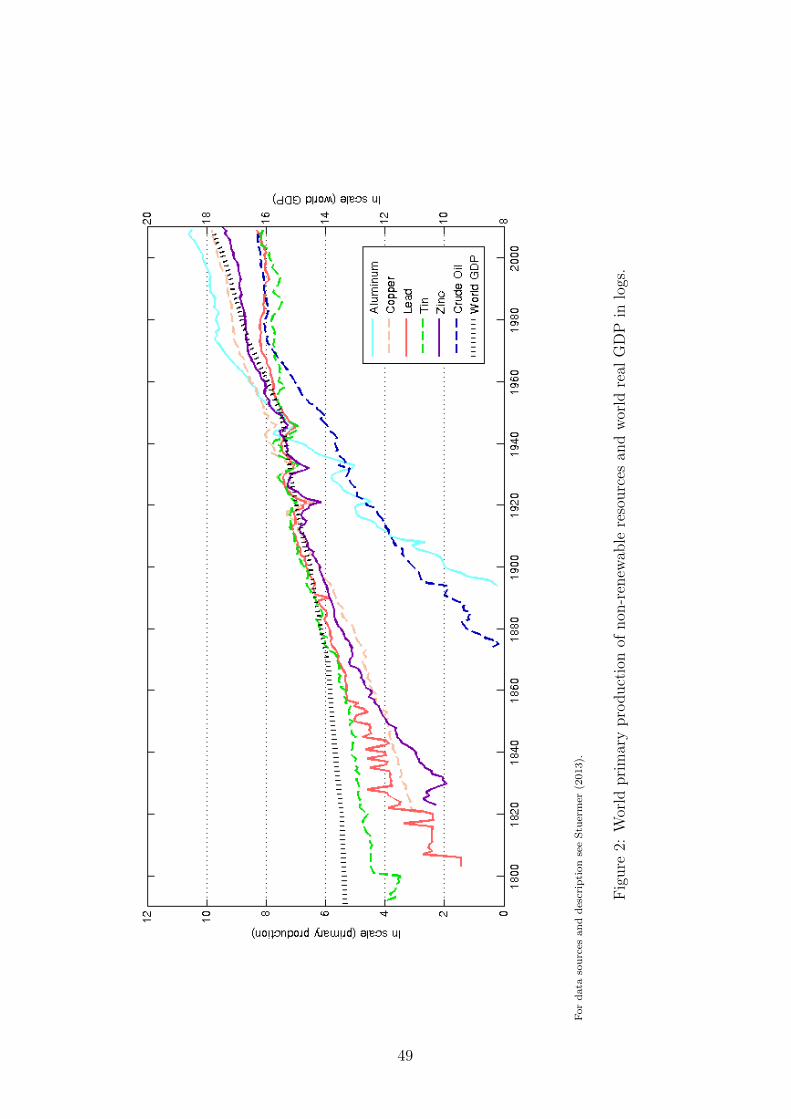
Figure 2 shows that the world primary production of the examined non-renewable

resources and world real GDP approximately exhibit constant positive growth rates

since 1792. A closer statistical examination confirms that the production of non-

renewable resources exhibits significantly positive growth rates in the long term (see

8

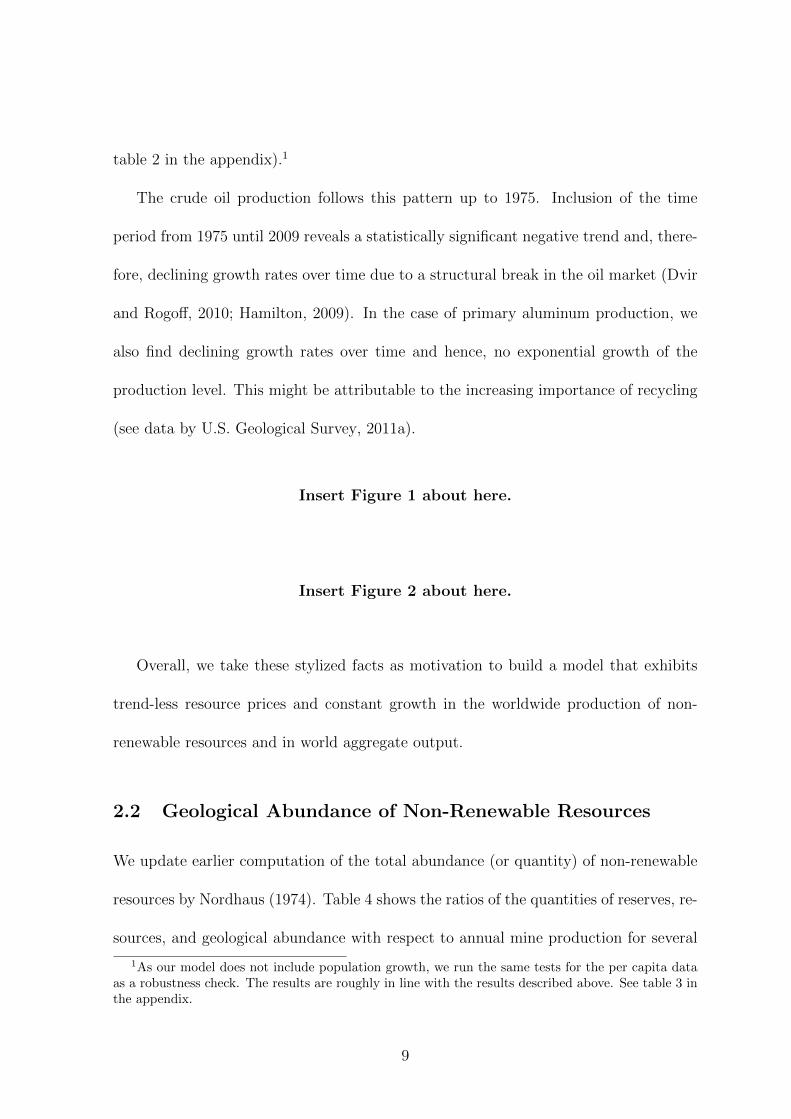
table 2 in the appendix).1

The crude oil production follows this pattern up to 1975. Inclusion of the time

period from 1975 until 2009 reveals a statistically significant negative trend and, there-

fore, declining growth rates over time due to a structural break in the oil market (Dvir

and Rogo↵, 2010; Hamilton, 2009). In the case of primary aluminum production, we

also find declining growth rates over time and hence, no exponential growth of the

production level. This might be attributable to the increasing importance of recycling

(see data by U.S. Geological Survey, 2011a).

Insert Figure 1 about here.


Overall, we take these stylized facts as motivation to build a model that exhibits

trend-less resource prices and constant growth in the worldwide production of non-

renewable resources and in world aggregate output.

2.2 Geological Abundance of Non-Renewable Resources

We update earlier computation of the total abundance (or quantity) of non-renewable

resources by Nordhaus (1974). Table 4 shows the ratios of the quantities of reserves, re-

sources, and geological abundance with respect to annual mine production for several

1As our model does not include population growth, we run the same tests for the per capita dataas a robustness check. The results are roughly in line with the results described above. See table 3 inthe appendix.

9

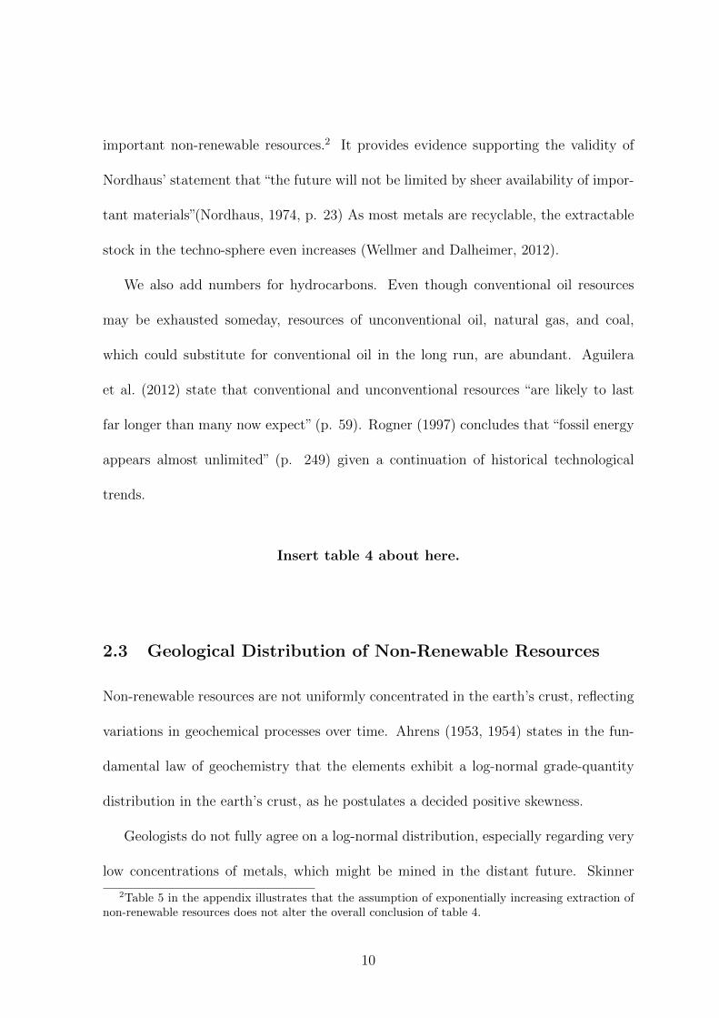
important non-renewable resources.2 It provides evidence supporting the validity of

Nordhaus’ statement that “the future will not be limited by sheer availability of impor-

tant materials”(Nordhaus, 1974, p. 23) As most metals are recyclable, the extractable

stock in the techno-sphere even increases (Wellmer and Dalheimer, 2012).

We also add numbers for hydrocarbons. Even though conventional oil resources

may be exhausted someday, resources of unconventional oil, natural gas, and coal,

which could substitute for conventional oil in the long run, are abundant. Aguilera

et al. (2012) state that conventional and unconventional resources “are likely to last

far longer than many now expect” (p. 59). Rogner (1997) concludes that “fossil energy

appears almost unlimited” (p. 249) given a continuation of historical technological

trends.

Insert table 4 about here.

2.3 Geological Distribution of Non-Renewable Resources

Non-renewable resources are not uniformly concentrated in the earth’s crust, reflecting

variations in geochemical processes over time. Ahrens (1953, 1954) states in the fun-

damental law of geochemistry that the elements exhibit a log-normal grade-quantity

distribution in the earth’s crust, as he postulates a decided positive skewness.

Geologists do not fully agree on a log-normal distribution, especially regarding very

low concentrations of metals, which might be mined in the distant future. Skinner

2Table 5 in the appendix illustrates that the assumption of exponentially increasing extraction ofnon-renewable resources does not alter the overall conclusion of table 4.

10

(1979) and Gordon et al. (2007) propose a discontinuity in the distribution due to the

so-called “mineralogical barrier,” the approximate point below which metal atoms are

trapped by atomic substitution.

Gerst (2008) concludes in his geological study of copper deposits that he can neither

confirm nor refute these two hypotheses. However, based on worldwide data on copper

deposits over the past 200 years, he finds evidence for a log-normal relationship between

copper production and ore grades. Mudd (2007) analyzes the historical evolution of

extraction and grades of deposits for di↵erent base metals in Australia. He finds that

production has increased at a constant rate, while grades have consistently declined.

We recognize that there remains uncertainty about the geological distribution, es-

pecially regarding hydrocarbons with their distinct formation processes. However, we

believe that it is reasonable to assume that a non-renewable resource is distributed

according to a log-normal relationship between the grade of deposits and quantity.

2.4 Technological Change in the Extractive Sector

Technological change in resource extraction o↵sets the depletion of economically ex-

tractable reserves of non-renewable resources (Simpson, 1999, and others). Hence,

reserves are drawn down by extraction, but increase by technological change in ex-

traction technology. The reason for this phenomenon is that non-renewable resources

such as copper, aluminum, and hydrocarbons are extractable at di↵erent costs due to

varying grades, thickness, depths, and other characteristics of mineral deposits. Tech-

nological change makes deposits economically extractable that, due to high costs, have

not been previously extractable (see Simpson, 1999; Nordhaus, 1974, and others).

11

There is ample empirical and narrative evidence for this phenomenon (see for ex-

ample Lasserre and Ouellette, 1991; Mudd, 2007; Simpson, 1999; Wellmer, 2008). For

example, Radetzki (2009) and Bartos (2002) describe how technological changes in

mining equipment, prospecting, and metallurgy have gradually made possible the ex-

traction of copper from lower grade deposits. Figure 4 shows that copper reserves3

have increased by more than 700 percent over the last couple of decades. As a con-

sequence, the average ore grades of copper mines, for example, have decreased from

about twenty percent 5,000 years ago to currently below one percent (Radetzki, 2009).

Figure 3 illustrates this development using the example of U.S. copper mines.

Gerst (2008) and Mudd (2007) come to similar results for worldwide copper mines

and the mining of di↵erent base-metals in Australia. The evidence also shows that

decreases in average mined ore grades have slowed as technological development pro-

gressed. Under the assumption that global R&D investment has stayed constant or

increased in real terms, this suggests that there are decreasing returns to R&D in

terms of making mining from deposits of lower grades economically feasible.



We observe similar developments for hydrocarbons. Using the example of the o↵-

shore oil industry, Managi et al. (2004) show that technological change has o↵set the

3Reserves are those resources for which extraction is considered economically feasible (U.S. Geo-logical Survey, 2011c).

12

cost-increasing degradation of resources. Crude oil has been extracted from ever deeper

sources in the Gulf of Mexico, as Figure 5 in the appendix shows. Furthermore, tech-

nological change and high prices have made it profitable to extract hydrocarbons from

unconventional sources, such as light tight oil, oil sands, and liquid natural gas (Inter-

national Energy Agency, 2012). As a result, oil reserves have doubled since the 1980s

(see figure 6 in the appendix).

Overall, empirical evidence suggests that technological change o↵sets resource de-

pletion by increasing economically extractable reserves. History shows that average

ore grades of mines declined while technological development progressed. Evidence

suggests that the e↵ect of technological change has slowed down in terms of making

deposits of lower grades economically extractable.

3 The Model

We build an endogenous growth model with two sectors, an extractive sector and an

intermediate goods sector, and take the framework by Acemoglu (2002) as a starting

point.

3.1 The Setup

We consider a standard setup of an economy with a representative consumer that has

constant relative risk aversion preferences:4

Z 1

0

C

1�✓t

� 1

1� ✓

e

�⇢tdt . (1)

4For a social planner version of the model, see the online appendix.

13

The variable Ct

denotes the consumption of aggregate output at time t, ⇢ is the discount

rate, and ✓ is the coe�cient of relative risk aversion. To ease notation, we drop time

indexes, whenever possible. The budget constraint of the representative consumer is:

C + I +M Y ⌘h�Z

"�1" + (1� �)R

"�1"

i ""�1

. (2)

On the left hand side, C denotes consumption, I is aggregate investment in produc-

tion, and M denotes aggregate R&D investment both in the extractive sector and the

intermediate goods sector, where M = M

Z

+M

R

. The usual no-Ponzi game conditions

apply.

On the right hand side, aggregate output production uses the non-renewable re-

source R, produced by the extractive sector, and an intermediate good Z, produced

by the intermediate goods sector. The distribution parameter � 2 (0, 1) indicates their

respective importance in producing aggregate output Y . The elasticity of substitution

between the resource and the intermediate good is denoted by ✏ 2 (0,1).

3.2 The Extractive Sector

There is an infinite number of infinitely small extractive firms i, which produce the

non-renewable resource from a geological environment.5

5For an alternative version of the extraction sector (using an approach analogous to the machinetypes in the intermediate sector) see the online appendix.

14

3.2.1 Geology

The geological environment consists of a continuum of deposits of declining grades

d 2 [0, 1], which contain the non-renewable resource R. Mineral deposits exhibit a

multitude of characteristics that a↵ect extraction cost. However, we concentrate on the

grade of deposits. Grade d refers to a measure of quality of the deposits, for example,

ore grades in the case of metals. It may also point to di↵erent types of deposits of

hydrocarbons. For example, we could say that conventional crude oil is extracted from

high grade deposits, while unconventional crude oil is produced from low grade deposits.

Grade d = 1 corresponds to a deposit, which is extractable without any technology.

For example, 7,000 years ago humans picked-up high-grade copper nuggets from the

ground. A deposit of grade zero does not contain any of the non-renewable resource.

We take a local approximation of the log-normal grade-quantity distribution pro-

posed by Ahrens (1953, 1954) (see chapter 2). We assume that the resource quantity

D is a function of the grade d of its deposits according to:

D(d) = ��1 ln(d), �1 2 R+ , (3)

This functional form is also in line with above described historical evidence that the

total quantity of non-renewable resource production has been inversely proportional to

the grades of the deposits. We assume that this relationship is continuous to hold in a

time-frame that is relevant to economic decision-making. The functional form therefore

implies that the quantity of the resource becomes infinitely large for deposits of small

grades.

15

Parameter �1 controls the curvature of the function. If �1 is high, the marginal

e↵ect on the quantity of the non-resources from shifting to deposits of lower grades is

high. It implies that the average concentration of the non-renewable resource is high

in the crustal mass (see also figure 7).


3.2.2 Extraction Technology

Firms fully know about the deposits and the geological distribution of the resource

quantity by grade. Firms invest MR

in terms of total output to develop grade specific

extraction technology and to convert deposits of a specific grade into economically

extractable reserves. Firms can extract the non-renewable resource from reserves at a

constant operational cost. We assume that the operational cost for deposits that are

not classified as reserves is infinitely high.

Each deposit of a certain grade d is associated with a unique state of the accumu-

lated extraction technology N

R

. Technology in the extractive sector is thus vertical.

The grade specific technology di↵uses directly after the invention, but allows a firm to

claim all of the non-renewable resource in the respective deposit. The assumption of

technology di↵usion is reasonable for the long-run and for the global perspective of our

model, as patent protection is often not available or enforced. In oil production, for

example, firms are obliged by law to make partially public the ingredients of fracking

new wells.

16

Based on the stylized facts in chapter 2, we assume that technological development

makes deposits economically extractable, but that there are decreasing returns in terms

of ore grades. We therefore assume the following extraction technology function h:

h(NR

) = e

��2NR, �2 2 R+ . (4)

Figure 8 shows the function. It shows how an increase in the stock of mining

technology N

R

makes deposits of certain grades extractable. The curve starts with

deposits of 100 percent ore grade, which represents the state of the world several

thousand years ago. The functional form is roughly in line with historical data for

U.S. copper mining over the last 100 years, as presented in Figure 3. We assume this

relationship holds continuous in a time-frame that is relevant to economic decision

making. We presume that ore grades only get closer to zero in the long term.

The marginal e↵ect of the extraction technology on converting deposits to econom-

ically extractable reserves declines as grades decrease. �2 is the curvature parameter

of the extraction technology function. If, for example, �2 is high, the average e↵ect of

new technology on converting deposits to reserves in terms of grades is relatively high.


We make use of a simple extraction cost function. Each deposit of a certain grade

d

N

is associated with a unique state of the technology, above which the deposit can be

extracted at cost �NR = E. Extraction is impossible at grades lower than d

N

, because

the cost is assumed to be infinite.

17

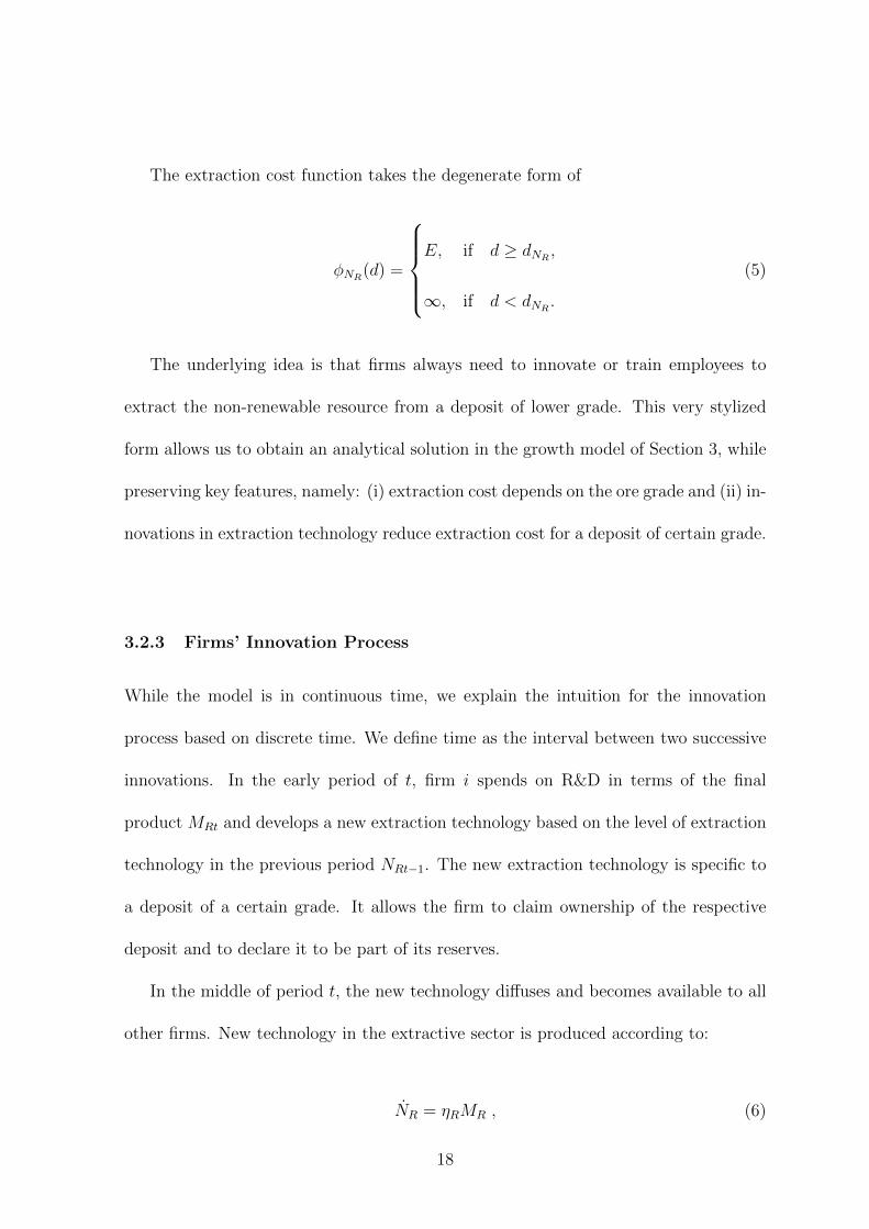
The extraction cost function takes the degenerate form of

�

NR(d) =

8>>><

>>>:

E, if d � d

NR ,

1, if d < d

NR .

(5)

The underlying idea is that firms always need to innovate or train employees to

extract the non-renewable resource from a deposit of lower grade. This very stylized

form allows us to obtain an analytical solution in the growth model of Section 3, while

preserving key features, namely: (i) extraction cost depends on the ore grade and (ii) in-

novations in extraction technology reduce extraction cost for a deposit of certain grade.

3.2.3 Firms’ Innovation Process

While the model is in continuous time, we explain the intuition for the innovation

process based on discrete time. We define time as the interval between two successive

innovations. In the early period of t, firm i spends on R&D in terms of the final

product MRt

and develops a new extraction technology based on the level of extraction

technology in the previous period N

Rt�1. The new extraction technology is specific to

a deposit of a certain grade. It allows the firm to claim ownership of the respective

deposit and to declare it to be part of its reserves.

In the middle of period t, the new technology di↵uses and becomes available to all

other firms. New technology in the extractive sector is produced according to:

N

R

= ⌘

R

M

R

, (6)

18

where ⌘R

is a cost parameter of technological innovation. One unit of final good spent

on R&D will produce ⌘R

new technologies. Technology is derived from R&D investment

in a deterministic way. This reflects a long-term perspective.

In the late period of t, the firm decides whether to extract the non-renewable re-

source from its reserves and sell it. Firms take the price of the non-renewable resource,

p

R

, as given. There is perfect competition due to free market entry and a linear pro-

duction technology.6 One firm extracts the resource at any given point in time.

3.2.4 Firms’ Optimization Problem

Firms in the extractive sector invest in new extraction technology despite the fully

competitive environment, because technology is grade specific. As soon as the cost of

developing a lower-grade technology can be paid for by revenues, firms will invest.

As new technology is specific to a deposit of a certain grade and benefits di↵use

within one period, firms maximize only current profits when making their technology

investment decisions. They generate just enough revenue from selling the resource R

at the given price p

R

to cover the R&D spending on extraction technology M

R

. Firms

have operational costs �NR for extracting one unit of the non-renewable resource. Firms

make zero profits while innovating. Each extraction firm solves a static optimization

problem, where the firm chooses investment into extraction technology optimally:

6We believe that perfect competition is a sensible assumption for non-renewable resource marketsin the long run. There is ample evidence that this is the case when looking at these markets over along period, as supply is elastic in the long run (see e.g. Radetzki, 2008). Perfect competition in theextraction sector results from the inexhaustible character of the resource. If one firm demands a priceabove marginal cost, another firm can develop additional technology, extract the resource from lowerore grades and sell it at a lower price in the long run.

19

maxR

p

R

R� �

NRR�M

R

. (7)

Most similar to this understanding of innovation is Desmet and Rossi-Hansberg

(2014), where non-replicable factors of production ensure technological development

in a perfectly competitive environment. In our case these non-replicable factors are

deposits of a specific grade.

Boiling down a dynamic optimization problem to a static one is key to our theory. It

allows us to make the model solvable and computable. At the same time, the model is

rich enough to derive meaningful theoretical predictions about the relationship between

technological change, geology and economic growth.

Each extractive firm’s reserves evolve according to:

S

t

= X

t

�R

t

, S

t

� 0, Xt

� 0, Rt

� 0 , (8)

A change in the resource quantity in reserves S is the result of two flows: (i) inflows of

new resource quantities X due to technology investment that convert mineral deposits

into reserves, and (ii) outflows of resource quantities R due to extraction and marketing.

Rearranging equation (8), we obtain the production function of the extractive sec-

tor:

R

t

= X

t

� S

t

. (9)

Note that for Xt

= 0, this formulation is the standard Hotelling (1931) setup.

20

3.3 The Intermediate Goods Sector

The intermediate goods sector follows the basic setup of Acemoglu (2002). Firms

produce an intermediate good Z according to the following production function:7

Z =1

1� �

✓ZNz

0

x

z

(j)1��dj

◆L

�

, (10)

where � 2 (0, 1). Firms use labor L, which is in fixed supply, and machines as inputs

to production. x

Z

(j) refers to the number of machines used for each machine variety

j. Machines depreciate fully within one period. We denote the range of machines that

can be used for production by N

z

. The intermediate good market is competitive. The

maximization problem of firms in the intermediate goods sector is:

maxL,{xZ(j)}

p

Z

Z � wL�Z

NZ

0

�

Z

(j)xZ

(j)dj , (11)

where p

Z

denotes the price of the intermediate good, w is the wage rate, and �

Z

(j)

refers to the rental rate for machine type j.

Sector-specific technology firms invent new technologies for which they hold a fully

enforceable patent. They exploit the patent by becoming the sole supplier of the ma-

chine that corresponds uniquely to their technology. The uniqueness provides market

power that they can use to set a price �Z

(j) above marginal cost. This allows them to

derive profits and to finance innovation. The marginal cost of producing a patent for

a new machine in terms of the final good is the same for all machines.

7Like Acemoglu (2002) we assume that the firm level production functions exhibit constant returnsto scale, so there is no loss of generality in focusing on the aggregate production functions.

21

Technology firms in the intermediate goods sector invent new varieties of machines

N

Z

according to

N

Z

= ⌘

Z

M

Z

, (12)

where M

Z

is R&D investment by the technology firms in terms of the final product,

and ⌘

Z

is a cost parameter. For more details, the reader is referred to the appendix

and Acemoglu (2002).

4 Theoretical Implications

We derive six propositions on the interaction between geology and technology and its

impact on the resource price, total output, and the resource intensity of the economy.8

First, the geological function, equation (3), and the technological function, equation

(equation 4), have o↵setting e↵ects. Extraction firms therefore face constant R&D costs

in converting one unit of the resource from a deposit into a new reserve.

Proposition 1 The total resource quantity converted to economically extractable re-

serves develops proportionally to the level of extraction technology N

R

:

D(h(NRt

)) = �1�2NRt

. (13)

The marginal return on extraction technology, NR

, in terms of resource quantities in

new reserves, X, is constant due to o↵setting interaction between technological change

8Proofs for this section are in the Appendix.

22

and geology: (i) new extraction technology exhibits decreasing returns in terms of mak-

ing lower grade deposits extractable; (2) the resource quantity is geologically distributed

such that it implies increasing returns in terms of resource quantities as the grade of

its deposits declines.

X

t

=@D(h(N

Rt

))

@t

= �1�2NRt

. (14)

Equation 14 depends on the shapes of the geological function and the technology

function. If the respective parameters �1 and �2 are high, the marginal return on new

extraction technology will also be high.

The marginal e↵ect of R&D investment on new reserves in terms of resource quan-

tities is also constant. Using equations (6) and (14), we can show that new reserves

X develop in proportion to R&D investment in extraction technology M

R

= 1⌘RN

R

=

1⌘R�1�2

X

t

.

Second, since the marginal e↵ect of R&D investment on new reserves is constant,

extractive firms’ optimization yields the typical result of stock management: inflows

and outflows into reserves balance over time.

Proposition 2 Firms increase the quantity of resources in their reserves due to R&D

in extraction technology X. This equals resource extraction R: X

t

= R

t

.

If we assume stochastic technological change, extractive firms will keep a positive

stock of reserves St

to insure against a series of bad draws in R&D. Reserves will grow

over time in line with aggregate growth. Proposition 2 would, however, remain the

same: In the long term, resource extraction equals resources in new reserves.

23

Third, the resource price equals marginal production costs due to perfect compe-

tition in the resource market. Firms’ marginal production costs consist of their R&D

cost for converting one unit of the resource into new reserves, if we set operational cost

to zero �NR = 0.

Proposition 3 The resource price depends negatively on the average crustal concen-

tration of the non-renewable resource and the average e↵ect of extraction technology:

p

Rt

=1

⌘

R

�1�2. (15)

The intuition is as follows: If, for example, �1 increases, the average crustal concen-

tration of the resource increases (see equation (3)) and the price decreases. If �2 rises,

the average e↵ect of new extraction technology on converting deposits of lower grades

to reserves increases (see equation (4)). This implies lower prices. The resource price

level also depends negatively on the cost parameter of R&D development ⌘R

.

Fourth, substituting equation (15) into the resource demand equation (18) in the

appendix, we obtain the ratio of resource consumption to aggregate output.

Proposition 4 The resource intensity of the economy is positively a↵ected by the aver-

age crustal concentration of the resource and the average e↵ect of extraction technology:

R

Y

= [(1� �)⌘R

�1�2]"

.

24

The elasticity of substitution has a strong negative impact on the resource intensity. If

the resource and the intermediate good are complements, ✏ < 1, the resource intensity

of the economy is relatively high and the resource price is relatively low compared to

the intermediate goods price. If they are substitutes, ✏ > 1, the resource intensity is

significantly lower and the relative resource price is high. The resource intensity also

depends positively on parameter �, which governs the importance of the resource in

the aggregate production function.

Fifth, we turn to the solution of the model. Adding the extractive sector to the

standard model by Acemoglu (2002), changes the interest part of the Euler equation,

g = ✓

�1(r�⇢).9 Instead of two exogenous production factors, the interest rate r in our

model only includes labor, but adds the resource price.

Proposition 5 The growth rate on the balanced growth path of the economy is constant

and given by

g = ✓

�1

0

@�⌘

Z

L

"�

�" �✓1� �

�

◆"

✓1

⌘

R

�1�2

◆1�"# 1

1�"1�

� ⇢

1

A.

The growth rate of the economy depends positively on the average geological concen-

tration of the resource, �1, and the average e↵ect of extractive technology in terms of

lower grades, �2.10

9There is no capital in this model, but agents delay consumption by investing in R&D as a functionof the interest rate.

10When the elasticity of substitution is low and the resource price is high (such that ��" <⇣1��

⌘" ⇣1

⌘R�1�2

⌘1�"a “limits to growth” situation occurs. There is no solution to equation (28)

in this case. The intuition is that developing new technologies to make new reserves extractable isextremely di�cult and substituting the resource by intermediate goods is only limited. Aggregateoutput production may therefore be impossible (see also Dasgupta and Heal, 1979, p. 196).

25

Finally, we derive the growth rates of technology in the two sectors. The stock of

technology in the intermediate goods sector grows at the same rate as the economy.

Proposition 6 The stock of extraction technology grows proportionally to output ac-

cording to:

N

R

= ⌘

R

M

Rt

= (�1�2)"�1(1� �)"⌘

R

Y .

In contrast to the intermediate goods sector, where firms can make use of the en-

tire stock of technology, firms in the extractive sector can only use the flow of new

technology to convert deposits of lower grades into new reserves. Previously devel-

oped technology cannot be employed because it is grade specific, and deposits of that

particular grade have already been depleted. Note also that firms in the extractive

sector need to invest a larger share of total output to attain the same rate of growth

in technology in comparison as firms in the intermediate goods sector.

The e↵ects of the two parameters �1 from the geological function and �2 from the

extraction technology function on N

R

depend on the elasticity of substitution ". If

✏ < 1, the resource and the intermediate good are gross complements, and increases in

�1 or �2 a↵ect NR

negatively. If the two goods are gross substitutes, higher parameter

values for �1 or �2 lead to more R&D investment in the extractive sector and hence a

higher rate of technological development in the extractive sector.

4.1 Discussion

We discuss the assumptions made in section 3, the comparison to the other models with

non-renewable resources, and the question of the ultimate finiteness of the resource.

26

How would other functional forms of the geological function in equation (3) a↵ect

the predictions of the model? First, the predictions are valid for all parameter values

�1 2 R+. Secondly, if D is discontinuous with an unanticipated break at d0, at which

the parameter changes to �01 2 R+, there would be two balanced growth paths: one for

the period before, and one for the period after the break. Both paths would behave

according to the model’s predictions. The paths would di↵er in the extraction cost of

producing the resource, level of extraction, and use of the resource in the economy.

To see this, recall from proposition 1 that X

t

is a function of �1. A non-exponential

form of D would produce results that di↵er from ours. It could feature a scarcity

rent as in the Hotelling (1931) model, as a non-exponential form of D would cause a

positive trend in resource prices. The extraction of deposits of lower ore grade might

also become infeasible. In these cases, the extractive firms consider the opportunity

cost of extracting the resource in the future, in addition to extraction and innovation

cost. Note that such a scarcity rent has not yet been found empirically (see e.g. Hart

and Spiro, 2011).

How does our model compare to other models with non-renewable resources? We

make the convenient assumption that the quantity of non-renewable resources is for all

practical economic purposes infinite. As a consequence, resource availability does not

limit growth. Substitution of capital for non-renewable resources, technological change

in the use of the resource, and increasing returns to scale are therefore not necessary for

sustained growth as in Groth (2007) or Aghion and Howitt (1998). If the resource were

finite in our model, the extractive sector would behave in the same way as in standard

models with a sector based on Hotelling (1931). As Dasgupta and Heal (1980) point

27

out, in this case the growth rate of the economy depends strongly on the degree of

substitution between the resource and other economic inputs. For " > 1, the resource

is non-essential; for " < 1, the total output that the economy is capable of producing

is finite. The production function is, therefore, only interesting for the Cobb-Douglas

case.

Our model suggests that the non-renewable resource can be thought of as a form of

capital: if the extractive firms invest in R&D in extraction technology, the resource is

extractable without limits as an input to aggregate production. This feature marks a

distinctive di↵erence from models such as the one of Bretschger and Smulders (2012).

They investigate the e↵ect of various assumptions about substitutability and a decen-

tralized market on long-run growth, but keep the assumption of a finite non-renewable

resource. Without this assumption, the elasticity of substitution between the non-

renewable resource and other input factors is no longer central to the analysis of limits

to growth.

Some might argue that the relationship described in proposition 1 cannot continue

to hold in the future as the amount of non-renewable resources in the earth’s crust is

ultimately finite. Scarcity will become increasingly important, and the scarcity rent

will be positive even in the present. However, for understanding current prices and

consumption patterns, current expectations about future developments are important.

Given that the quantities of available resources indicated in table 4 are very large,

their ultimate end far in the future should not a↵ect behavior today. The relationship

described in proposition 1 seems to have held in the past and looks likely to hold for the

foreseeable future. Since in the long term, extracted resources equal the resources added

28

to reserves due to R&D in extraction technology, the price for a unit of the resource

will equal the extraction cost plus the per-unit cost of R&D and hence, stay constant

in the long term. This may explain why scarcity rents cannot be found empirically.

5 Conclusion

This paper examines interaction between geology and technology and its impact on

the resource price, total output growth, and the resource intensity of the economy.

We argue that economic growth causes the production and use of a non-renewable

resource to increase at a constant rate. Marginal production costs stay constant in

the long term. Economic growth enables firms to invest in extraction technology R&D,

which makes resources from deposits of lower grades economically extractable. We help

explain the long-term evolution of non-renewable resource prices and world production

for more than 200 years. If historical trends in technological progress continue, it is

possible that non-renewable resources are, within a time frame relevant for humanity,

practically inexhaustible.

Our model makes strong simplifying assumptions, which render our model analyti-

cally solvable. However, we believe that a less simple model would essentially provide

the same results. There are four major simplifications, which should be examined in

more detail in future extensions. First, there is no uncertainty in R&D development,

and therefore no incentive for firms to keep a positive amount of the non-renewable

resource in their reserves. If R&D development is stochastic as in Dasgupta and Stiglitz

(1981), there would be a need for firms to keep reserves.

29

Second, our model features perfect competition in the extractive sector. We could

obtain a model with monopolistic competition in the extractive sector by introducing

explicitly privately-owned deposits. A firm would need to pay a certain upfront cost

or exploration cost in order to acquire a mineral deposit. This upfront cost would give

technology firms a certain monopoly power as they develop machines that are specific

to a single deposit.

Third, extractive firms could face a trade-o↵ between accepting high extraction

costs due to a lower technology level and investing in R&D to reduce extraction costs.

A more general extraction technology function would provide the basis to generalize

this assumption.

Fourth, our model does not include recycling. Recycling has become more important

for metal production over time due to the increasing abundance of recyclable materials

and the comparatively low energy requirements (see Wellmer and Dalheimer, 2012).

Introducing recycling into our model would further strengthen our argument, as it

increases the economically extractable stock of the non-renewable resource.

30

Appendix 1 Proofs

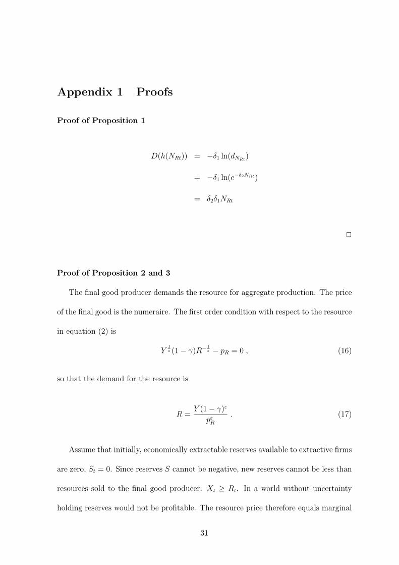
Proof of Proposition 1

D(h(NRt

)) = ��1 ln(dNRt)

= ��1 ln(e��2NRt)

= �2�1NRt

2

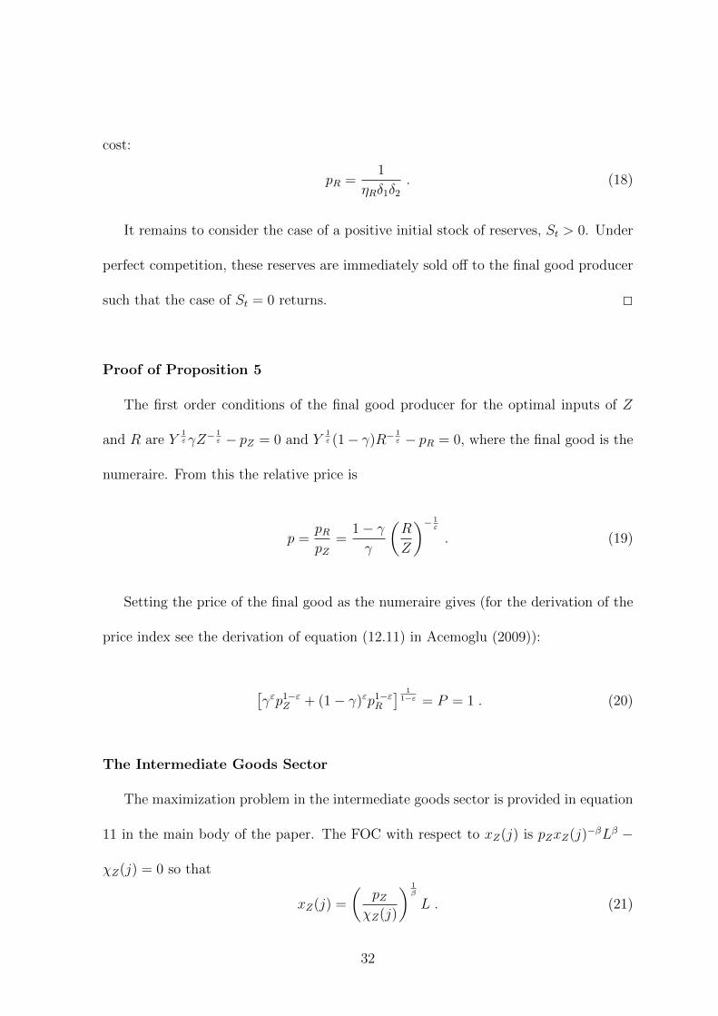
Proof of Proposition 2 and 3

The final good producer demands the resource for aggregate production. The price

of the final good is the numeraire. The first order condition with respect to the resource

in equation (2) is

Y

1" (1� �)R� 1

" � p

R

= 0 , (16)

so that the demand for the resource is

R =Y (1� �)"

p

"

R

. (17)

Assume that initially, economically extractable reserves available to extractive firms

are zero, St

= 0. Since reserves S cannot be negative, new reserves cannot be less than

resources sold to the final good producer: X

t

� R

t

. In a world without uncertainty

holding reserves would not be profitable. The resource price therefore equals marginal

31

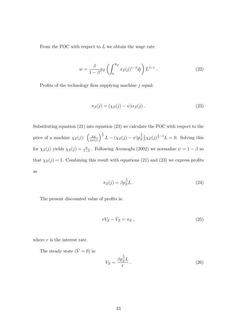
cost:

p

R

=1

⌘

R

�1�2. (18)

It remains to consider the case of a positive initial stock of reserves, St

> 0. Under

perfect competition, these reserves are immediately sold o↵ to the final good producer

such that the case of St

= 0 returns. 2


The first order conditions of the final good producer for the optimal inputs of Z

and R are Y

1"�Z

� 1" � p

Z

= 0 and Y

1" (1� �)R� 1

" � p

R

= 0, where the final good is the

numeraire. From this the relative price is

p =p

R

p

Z

=1� �

�

✓R

Z

◆� 1"

. (19)

Setting the price of the final good as the numeraire gives (for the derivation of the

price index see the derivation of equation (12.11) in Acemoglu (2009)):

⇥�

"

p

1�"Z

+ (1� �)"p1�"R

⇤ 11�" = P = 1 . (20)

The Intermediate Goods Sector

The maximization problem in the intermediate goods sector is provided in equation

11 in the main body of the paper. The FOC with respect to x

Z

(j) is pZ

x

Z

(j)��L� �

�

Z

(j) = 0 so that

x

Z

(j) =

✓p

Z

�

Z

(j)

◆ 1�

L . (21)

32

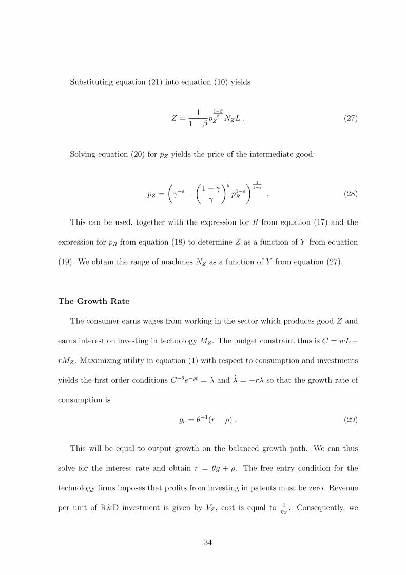
From the FOC with respect to L we obtain the wage rate

w =�

1� �

p

Z

✓ZNZ

0

x

Z

(j)1��dj

◆L

��1. (22)

Profits of the technology firm supplying machine j equal:

⇡

Z

(j) = (�Z

(j)� )xZ

(j) . (23)

Substituting equation (21) into equation (23) we calculate the FOC with respect to the

price of a machine �Z

(j):⇣

pZ

�Z(j)

⌘ 1�L � (�

Z

(j) � )p1�

Z

1�

�

Z

(j)1��1

L = 0. Solving this

for �Z

(j) yields �Z

(j) =

1�� . Following Acemoglu (2002) we normalize = 1� � so

that �Z

(j) = 1. Combining this result with equations (21) and (23) we express profits

as

⇡

Z

(j) = �p

1�

Z

L . (24)

The present discounted value of profits is:

rV

Z

� V

Z

= ⇡

Z

, (25)

where r is the interest rate.

The steady state (V = 0) is:

V

Z

=�p

1�

Z

L

r

. (26)

33

Substituting equation (21) into equation (10) yields

Z =1

1� �

p

1��

Z

N

Z

L . (27)

Solving equation (20) for pZ

yields the price of the intermediate good:

p

Z

=

✓�

�" �✓1� �

�

◆"

p

1�"R

◆ 11�"

. (28)

This can be used, together with the expression for R from equation (17) and the

expression for pR

from equation (18) to determine Z as a function of Y from equation

(19). We obtain the range of machines NZ

as a function of Y from equation (27).

The Growth Rate

The consumer earns wages from working in the sector which produces good Z and

earns interest on investing in technology M

Z

. The budget constraint thus is C = wL+

rM

Z

. Maximizing utility in equation (1) with respect to consumption and investments

yields the first order conditions C�✓e

�⇢t = � and � = �r� so that the growth rate of

consumption is

g

c

= ✓

�1(r � ⇢) . (29)

This will be equal to output growth on the balanced growth path. We can thus

solve for the interest rate and obtain r = ✓g + ⇢. The free entry condition for the

technology firms imposes that profits from investing in patents must be zero. Revenue

per unit of R&D investment is given by V

Z

, cost is equal to 1⌘Z. Consequently, we

34

obtain ⌘Z

V

Z

= 1. Making use of equation (26), we obtain⌘Z�p

1�Z L

r

= 1. Solving this for

r and substituting it into equation (29) we obtain:

g = ✓

�1(�⌘Z

Lp

1�

Z

� ⇢) . (30)

Together with Equations (18) and (28) this yields the growth rate on the balanced

growth path. 2


The expression for NR

follows from equation (14), proposition 2 and equation (17).

2

35

References

Acemoglu, D. (2002). Directed technical change. The Review of Economic Studies,

69(4):781–809.

Acemoglu, D. (2009). Introduction to modern economic growth. Princeton University

Press, Princeton, N.J.

Acemoglu, D., Aghion, P., Bursztyn, L., and Hemous, D. (2012). The environment and

directed technical change. American Economic Review, 102(1):131–66.

Aghion, P. and Howitt, P. (1998). Endogenous growth theory. MIT Press, London.

Aguilera, R., Eggert, R., Lagos C.C., G., and Tilton, J. (2012). Is depletion likely

to create significant scarcities of future petroleum resources? In Sinding-Larsen,

R. and Wellmer, F., editors, Non-renewable resource issues, pages 45–82. Springer

Netherlands, Dordrecht.

Ahrens, L. (1953). A fundamental law of geochemistry. Nature, 172:1148.

Ahrens, L. (1954). The lognormal distribution of the elements (a fundamental law of

geochemistry and its subsidiary). Geochimica et Cosmochimica Acta, 5(2):49–73.

Bartos, P. (2002). SX-EW copper and the technology cycle. Resources Policy, 28(3-

4):85–94.

Bretschger, L. and Smulders, S. (2012). Sustainability and substitution of exhaustible

natural resources: How structural change a↵ects long-term R&D investments. Jour-

nal of Economic Dynamics and Control, 36(4):536 – 549.

British Petroleum (2013). BP statistical review of world energy. http://www.bp.com/

(accessed on March 14, 2014).

Cynthia-Lin, C. and Wagner, G. (2007). Steady-state growth in a Hotelling model of re-

source extraction. Journal of Environmental Economics and Management, 54(1):68–

83.

Dasgupta, P. and Heal, G. (1979). Economic theory and exhaustible resources. Cam-

bridge Economic Handbooks (EUA).

Dasgupta, P. and Heal, G. (1980). Economic theory and exhaustible resources. Cam-

bridge University Press, Cambridge, U.K.

36

Dasgupta, P. and Stiglitz, J. (1981). Resource depletion under technological uncer-

tainty. Econometrica, 49(1):85–104.

Desmet, K. and Rossi-Hansberg, E. (2014). Innovation in space. American Economic

Review, 102(3):447–452.

Dvir, E. and Rogo↵, K. (2010). The three epochs of oil. mimeo.

Federal Institute for Geosciences and Natural Resources (2011). Reserven, Resourcen,

Verfugbarkeit von Energierohsto↵en 2011. Federal Institute for Geosciences and Nat-

ural Resources, Hanover, Germany.

Fourgeaud, C., Lenclud, B., and Michel, P. (1982). Technological renewal of natural

resource stocks. Journal of Economic Dynamics and Control, 4(1):1–36.

Gerst, M. (2008). Revisiting the cumulative grade-tonnage relationship for major cop-

per ore types. Economic Geology, 103(3):615.

Golosov, M., Hassler, J., Krusell, P., and Tsyvinski, A. (2014). Optimal taxes on fossil

fuel in general equilibrium. Econometrica, 82(1):41–88.

Gordon, R., Bertram, M., and Graedel, T. (2007). On the sustainability of metal

supplies: a response to Tilton and Lagos. Resources Policy, 32(1-2):24–28.

Groth, C. (2007). A new growth perspective on non-renewable resources. In Bretschger,

L. and Smulders, S., editors, Sustainable Resource Use and Economic Dynamics,

chapter 7, pages 127–163. Springer Netherlands, Dordrecht.

Hamilton, J. (2009). Understanding crude oil prices. The Energy Journal, 30(2):179–

206.

Hart, R. (2012). The economics of natural resources: understanding and predicting the

evolution of supply and demand. Working Paper of the Department of Economics

of the Swedish University of Agricultural Sciences, 1(3).

Hart, R. and Spiro, D. (2011). The elephant in Hotelling’s room. Energy Policy,

39(12):7834–7838.

Harvey, D. I., Kellard, N. M., Madsen, J. B., and Wohar, M. E. (2010). The Prebisch-

Singer hypothesis: four centuries of evidence. The Review of Economics and Statis-

tics, 92(2):367–377.

Hassler, J. and Sinn, H.-W. (2012). The fossil episode. Technical report, CESifo

Working Paper: Energy and Climate Economics.

37

Heal, G. (1976). The relationship between price and extraction cost for a resource with

a backstop technology. The Bell Journal of Economics, 7(2):371–378.

Hotelling, H. (1931). The economics of exhaustible resources. Journal of Political

Economy, 39(2):137–175.

International Energy Agency (2012). World energy outlook 2012. International Energy

Agency, Paris.

Jacks, D. S. (2013). From boom to bust: A typology of real commodity prices in the

long run. Technical report, National Bureau of Economic Research.

Krautkraemer, J. (1998). Nonrenewable resource scarcity. Journal of Economic Liter-

ature, 36(4):2065–2107.

Lasserre, P. and Ouellette, P. (1991). The measurement of productivity and scarcity

rents: the case of asbestos in canada. Journal of Econometrics, 48(3):287–312.

Lee, J., List, J., and Strazicich, M. (2006). Non-renewable resource prices: determin-

istic or stochastic trends? Journal of Environmental Economics and Management,

51(3):354–370.

Littke, R. and Welte, D. (1992). Hydrocarbon source rocks. Cambridge University

Press, Cambridge, U.K.

Livernois, J. (2009). On the empirical significance of the Hotelling rule. Review of

Environmental Economics and Policy, 3(1):22–41.

Managi, S., Opaluch, J., Jin, D., and Grigalunas, T. (2004). Technological change

and depletion in o↵shore oil and gas. Journal of Environmental Economics and

Management, 47(2):388–409.

Mudd, G. (2007). An analysis of historic production trends in australian base metal

mining. Ore Geology Reviews, 32(1):227–261.

Nordhaus, W. (1974). Resources as a constraint on growth. American Economic

Review, 64(2):22–26.

O�cer, L. (2011). Dollar-Pound exchange rate from 1791. MeasuringWorth.

O�cer, L. and Williamson, S. (2011). The annual consumer price index for the united

states, 1774-2010. http://www.measuringworth.com/uscpi/ (accessed November 2,

2011).

38

Perman, R., Yue, M., McGilvray, J., and Common, M. (2003). Natural resource and

environmental economics. Pearson Education, Edinburgh.

Pindyck, R. (1999). The long-run evolution of energy prices. The Energy Journal,

20(2):1–28.

Radetzki, M. (2008). A handbook of primary commodities in the global economy. Cam-

bridge Univ. Press, Cambridge, U.K.

Radetzki, M. (2009). Seven thousand years in the service of humanity: the history of

copper, the red metal. Resources Policy, 34(4):176–184.

Rogner, H. (1997). An assessment of world hydrocarbon resources. Annual Review of

Energy and the Environment, 22(1):217–262.

Scholz, R. and Wellmer, F. (2012). Approaching a dynamic view on the availability

of mineral resources: what we may learn from the case of phosphorus? Global

Environmental Change, 23(1):11–27.

Simon, J. (1981). The ultimate resource. Princeton University Press, Princeton, N.J.

Simpson, R., editor (1999). Productivity in natural resource industries: improvement

through innovation. RFF Press, Washington, D.C.

Skinner, B. (1979). A second iron age ahead? Studies in Environmental Science,

3:559–575.

Slade, M. (1982). Trends in natural-resource commodity prices: an analysis of the time

domain. Journal of Environmental Economics and Management, 9(2):122–137.

Stuermer, M. (2013). What drives mineral commodity markets in the long run?

PhD thesis, University of Bonn. http://hss.ulb.uni-bonn.de/2013/3313/3313.pdf (ac-

cessed September 4, 2013).

Stuermer, M. (2016). 150 years of boom and bust: What drives mineral commodity

prices? Macroeconomic Dynamics, forthcoming.

Tahvonen, O. and Salo, S. (2001). Economic growth and transitions between renewable

and nonrenewable energy resources. European Economic Review, 45(8):1379–1398.

Tilton, J. and Lagos C.C., G. (2007). Assessing the long-run availability of copper.

Resources Policy, 32(1-2):19–23.

39

U.S. Bureau of Labor Statistics (2010). Consumer price index. All urban consumers.

U.S. city average. All items.

U.S. Bureau of Mines (1991). Minerals yearbook. 1991. Metals and minerals. U.S.

Bureau of Mines, Washington, D.C.

U.S. Geological Survey (2010). Gold statistics. U.S. Geological Survey, Reston, V.A.

U.S. Geological Survey (2011a). Historical statistics for mineral and material com-

modities in the United States. U.S. Geological Survey, Reston, V.A.

U.S. Geological Survey (2011b). Mineral commodity summaries 2011. U.S. Geological

Survey, Reston, V.A.

U.S. Geological Survey (2011c). Minerals yearbook 2010. U.S. Geological Survey,

Reston, V.A.

U.S. Geological Survey (2012a). Historical statistics for mineral and material com-

modities in the United States. U.S. Geological Survey, Reston, V.A.

U.S. Geological Survey (2012b). Mineral commodity summaries 2012. U.S. Geological

Survey, Reston, V. A.

van der Ploeg, F. and Withagen, C. (2012). Too much coal, too little oil. Journal of

Public Economics, 96(1):62–77.

Von Hagen, J. (1989). Relative commodity prices and cointegration. Journal of Busi-

ness & Economic Statistics, 7(4):497–503.

Wellmer, F. (2008). Reserves and resources of the geosphere, terms so often misun-

derstood. Is the life index of reserves of natural resources a guide to the future.

Zeitschrift der Deutschen Gesellschaft fur Geowissenschaften, 159(4):575–590.

Wellmer, F. and Dalheimer, M. (2012). The feedback control cycle as regulator of past

and future mineral supply. Mineralium Deposita, 47:713–729.

40

Appendix 2 Tables

41

Aluminum Copper Lead Tin Zinc Crude Oil

Range 1905-2009 1792-2009 1792-2009 1792-2009 1824-2009 1862-2009Constant Coe↵. -1.774 0.572 0.150 1.800 1.072 8.242

t-stat. (-0.180) (0.203) (0.052) (0.660) (0.205) (0.828)Lin.Trend Coe↵. 0.008 0.009 0.016 0.001 0.014 -0.021

t-stat. (0.137) (0.428) (0.714) (0.069) (0.357) (-0.317)

Range 1905-2009 1850-2009 1850-2009 1862-2009 1850-2009 1850-2009Constant Coe↵. -1.299 0.109 -0.268 2.439 1.894 7.002

t-stat. (-0.200) (0.030) (-0.073) (0.711) (0.407) (1.112)Lin.Trend Coe↵. 0.008 0.020 0.030 -0.004 0.013 -0.021

t-stat. (0.137) (0.518) (0.755) (-0.109) (0.267) (-0.317)

Range 1900-2009 1900-2009 1900-2009 1900-2009 1900-2009 1900-2009Constant Coe↵. -0.903 -1.428 -0.490 1.068 2.764 -1.974

t-stat. (-0.239) (-0.332) (-0.102) (0.269) (0.443) (-0.338)Lin.Trend Coe↵. 0.008 0.055 0.054 0.010 0.010 0.100

t-stat. (0.137) (0.820) (0.713) (0.168) (0.099) (1.106)

Range 1950-2009 1950-2009 1950-2009 1950-2009 1950-2009 1950-2009Constant Coe↵. 2.269 1.556 -3.688 -0.061 -0.515 3.445

t-stat. (0.479) (0.240) (-0.505) (-0.011) (-0.062) (0.354)Lin.Trend Coe↵. -0.055 0.041 0.198 0.049 0.103 0.090

t-stat. (-0.411) (0.225) (0.958) (0.307) (0.441) (0.326)

Range 1875-1975 1875-1975 1875-1975 1875-1975 1875-1975 1875-1975Constant Coe↵. -0.549 1.323 0.370 3.719 1.136 -1.111

t-stat. (-0.088) (0.266) (0.081) (0.812) (0.176) (-0.176)Lin.Trend Coe↵. -0.003 0.011 0.030 -0.012 0.051 0.094

t-stat. (-0.033) (0.135) (0.383) (-0.152) (0.468) (0.875)

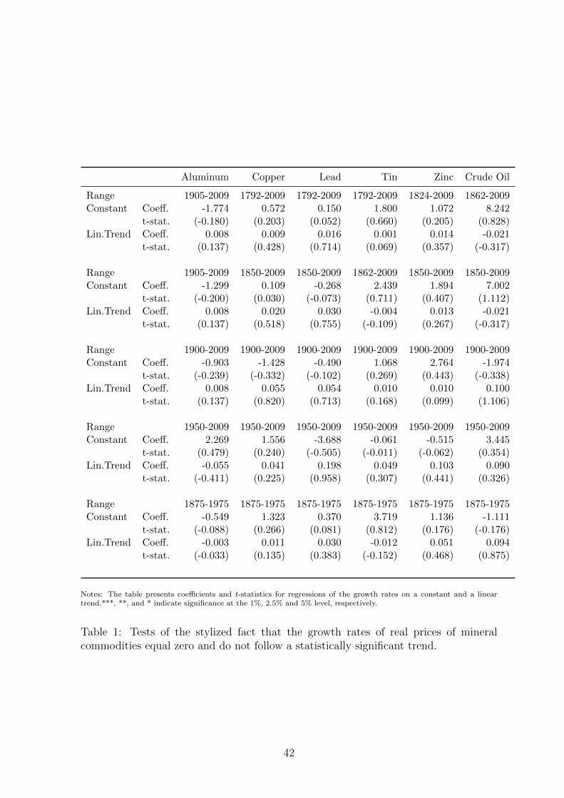
Notes: The table presents coe�cients and t-statistics for regressions of the growth rates on a constant and a lineartrend.***, **, and * indicate significance at the 1%, 2.5% and 5% level, respectively.

Table 1: Tests of the stylized fact that the growth rates of real prices of mineralcommodities equal zero and do not follow a statistically significant trend.

42

Aluminum Copper Lead Tin Zinc Crude Oil World GDP

Range 1855-2009 1821-2009 1802-2009 1792-2009 1821-2009 1861-2009 1792-2009Constant Coe↵. 48.464 4.86 16.045 4.552 30.801 35.734 0.128

t-stat. *** 3.810 *** 2.694 *** 3.275 * 2.231 ** 2.58 *** 4.365 0.959Lin.Trend Coe↵. -0.221 -0.006 -0.087 -0.016 -0.174 -0.182 0.018

t-stat. ** -2.568 -0.439 ** -2.294 -0.999 * -1.975 *** -3.334 *** 16.583


t-stat. *** 3.810 *** 3.461 ***3.371 * 2.185 *** 3.774 *** 4.81 *** 5.49Lin.Trend Coe↵. -0.221 -0.018 -0.038 -0.015 -0.021 -0.182 0.019

t-stat. ** -2.568 -1.007 -1.938 -0.833 -1.308 *** -3.334 *** 9.797


t-stat. *** 5.498 *** 2.651 * 2.043 1.361 * 2.225 *** 6.912 *** 7.8Trend Coe↵. -0.l78 0.035 -0.019 -0.015 -0.018 -0.083 0.018

t-stat. *** 3.174 -0.995 -0.853 -0.464 -0.592 ***-3.711 ***4.549


t-stat. *** 7.169 *** 4.979 *** 2.936 0.028 *** 4.619 *** 9.574 *** 12.89Lin.Trend Coe↵. -0.171 -0.057 -0.48 0.04 -0.078 -0.196 -0.028

t-stat. *** -3.999 -1.978 -1.553 0.768 * -2.255 *** -6.64 *** -2.724


t-stat. *** 4.846 ** 2.543 1.938 1.664 * 2.032 *** 4.060 *** 5.509Lin.Trend Coe↵. -0.53 -0.024 -0.018 -0.026 -0.005 -0.072 0.027

t-stat. *** -2.974 -0.566 -0.536 -0.66 -1.26 -1.403 ***7.045

Notes: The table presents coe�cients and t-statistics for regressions of the growth rates on a constant and a lineartrend. ***, **, and * indicate significance at the 1%, 2.5% and 5% level, respectively.

Table 2: Tests for the stylized facts that growth rates of world primary production andworld real GDP are equal to zero and trendless.

43

Aluminum Copper Lead Tin Zinc Crude Oil World GDP


t-stat. *** 3.824 *** 3.06 *** 3.845 * 2.181 ** 2.584 *** 4.379 0.276Lin.Trend Coe↵. -0.229 -0.018 -0.125 -0.023 -0.182 -0.19 0.01

t-stat. *** -2.677 -1.367 *** -3.025 -1.457 * -2.071 *** -3.499 *** 11.066


t-stat. *** 3.824 *** 3.254 ***3.169 1.961 *** 3.541 *** 4.733 *** 4.052Lin.Trend Coe↵. -0.229 -0.027 -0.047 -0.024 -0.03 -0.19 0.01

t-stat. *** -2.677 -1.523 ** -2.442 -1.348 -1.895 *** -3.499 *** 5.876


t-stat. *** 5.242 * 2.241 1.41 0.918 1.763 *** 6.306 *** 4.862Trend Coe↵. -0.l84 -0.042 -0.027 -0.023 -0.026 -0.09 0.01

t-stat. *** -3.315 -1.214 -1.186 -0.694 -0.404 *** -4.084 *** 3.01

Range 1950-2009 1950-2009 1950-2009 1950-2009 1950-2009 1950-2009 1950-2009Constant Coe↵. 8.583 2.952 1.141 -1.954 3.578 7.716 2.632

t-stat. *** 5.742 *** 2.892 1.04 1.086 *** 2.87 *** 7.493 *** 7.444Lin.Trend Coe↵. -0.156 -0.044 -0.35 0.051 -0.065 -0.18 -0.016

t-stat. *** -3.667 -1.515 -1.129 0.997 -1.819 *** -6.14 -1.551


t-stat. *** 4.81 ** 2.386 1.738 1.480 1.851 *** 3.933 *** 4.509Lin.Trend Coe↵. -0.542 -0.038 -0.032 -0.039 -0.019 -0.086 0.013

t-stat. *** -3.06 -0.908 -0.959 -1.028 -0.517 -1.691 ***4.004

Notes: The table presents coe�cients and t-statistics for regressions of the growth rates on a constant and a lineartrend. ***, **, and * indicate significance at the 1%, 2.5% and 5% level, respectively.

Table 3: Tests for the stylized fact that growth rates of world per capita primaryproduction and world per capita real GDP are equal to zero and trendless.

44

Reserves/ Resources/ Crustal abundance/

Annual production Annual production Annual production

(Years) (Years) (Years)

Aluminum 1391a 263,0001a 48,800,000,000bc

Copper 43a 189a 95,000,000ab

Iron 78a 223a 1,350,000,000ab

Lead 21a 362a 70.000.000ab

Tin 17a “Su�cient”a 144.000ab

Zinc 21a 158a 187.500.000ab

Gold 20d 13d 27,160,000ef

Rare earths2 827a “Very large”a n.a.Coal3 129g 2,900g

} 1,400,0006iCrude oil4 55g 76g

Gas5 59g 410g

Notes: Reserves include all material which can currently be extracted. The definition of resources can be found inSection 2.4. Sources: aU.S. Geological Survey (2012b), bPerman et al. (2003), cU.S. Geological Survey (2011c),dU.S.Geological Survey (2011b),eNordhaus (1974),fU.S. Geological Survey (2010), gFederal Institute for Geosciences andNatural Resources (2011) g

iLittke and Welte (1992). Notes: 1 data for bauxite, 2 rare earth oxide, 3 includes ligniteand hard coal, 4 includes conventional and unconventional oil, 5 includes conventional and unconventional gas, 6 allorganic carbon in the earth’s crust.

Table 4: Availability of selected non-renewable resources in years of production left inthe reserve, resource and crustal mass based on current annual mine production.

45

Reserves/ Resources/ Crustal abundance/

Annual production Annual production Annual production

(Years) (Years) (Years)

Aluminum 651ah 4191ah 838bch

Copper 30ag 77ag 718abg

Iron 44ah 78ah 744abh

Lead 18ah 181ah 1,907abh

Tin 18ah n.a. 3,588abh

Zinc 17ah 74ah 842abh

Gold 18dh 11dh 2,170efh

Rare earths2 127ah n.a. n.a.Coal3 65gk 215gk

} 7296jCrude oil4 46gk 60gk

Natural gas5 41gk 123gk

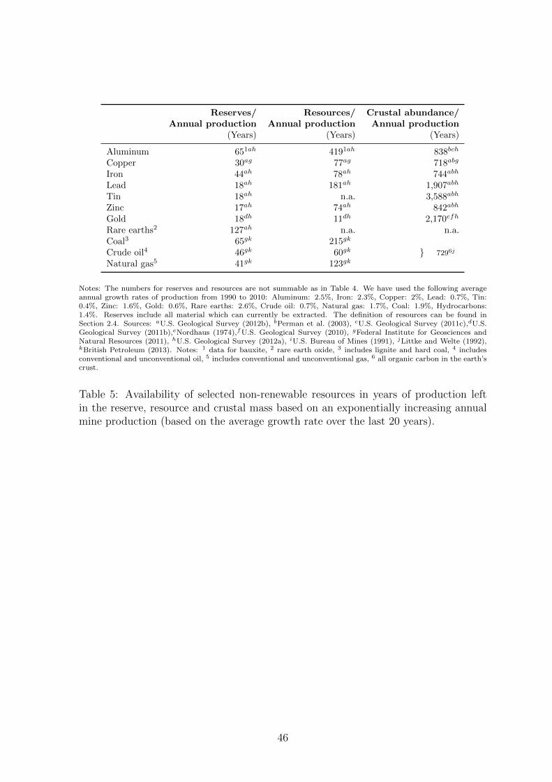
Notes: The numbers for reserves and resources are not summable as in Table 4. We have used the following averageannual growth rates of production from 1990 to 2010: Aluminum: 2.5%, Iron: 2.3%, Copper: 2%, Lead: 0.7%, Tin:0.4%, Zinc: 1.6%, Gold: 0.6%, Rare earths: 2.6%, Crude oil: 0.7%, Natural gas: 1.7%, Coal: 1.9%, Hydrocarbons:1.4%. Reserves include all material which can currently be extracted. The definition of resources can be found inSection 2.4. Sources: aU.S. Geological Survey (2012b), bPerman et al. (2003), cU.S. Geological Survey (2011c),dU.S.Geological Survey (2011b),eNordhaus (1974),fU.S. Geological Survey (2010), gFederal Institute for Geosciences andNatural Resources (2011), hU.S. Geological Survey (2012a), iU.S. Bureau of Mines (1991), jLittke and Welte (1992),kBritish Petroleum (2013). Notes: 1 data for bauxite, 2 rare earth oxide, 3 includes lignite and hard coal, 4 includesconventional and unconventional oil, 5 includes conventional and unconventional gas, 6 all organic carbon in the earth’scrust.

Table 5: Availability of selected non-renewable resources in years of production leftin the reserve, resource and crustal mass based on an exponentially increasing annualmine production (based on the average growth rate over the last 20 years).

46

Appendix 3 Figures

47

Notes:

All

prices,

exceptforth

eprice

ofcrudeoil,

are

pricesof

theLondon

MetalExch

ange

and

itspredecessors.

Asth

eprice

ofth

eLondon

MetalExch

angeused

tobe

den

ominatedin

Sterlingin

earliertimes,wehav

eco

nvertedth

esepricesto

U.S.-Dollarbyusinghistorica

lex

changeratesfrom

O�cer(2011

).W

euse

theU.S.-Con

sumer

Price

Index

provided

byO�cerandW

illiamson(2011

)an

dth

eU.S.Bureau

ofLaborStatistics(2010)

fordefl

atingpriceswithth

ebase

yea

r198

0-82.Theseco

ndary

y-axis

relatesto

theprice

ofcrudeoil.Fordatasources

anddescriptionseeStu

ermer

(2013).

Figure

1:Realpricesof

majormineral

commod

itiesin

naturallogs.

48

Fordata

sources

anddescriptionseeStu

ermer

(201

3).

Figure

2:World

primaryproductionof

non

-renew

able

resources

andworld

real

GDPin

logs.

49

Figure 3: The historical development of mining of various grades of copper in the U.S.Source: Scholz and Wellmer (2012)

50

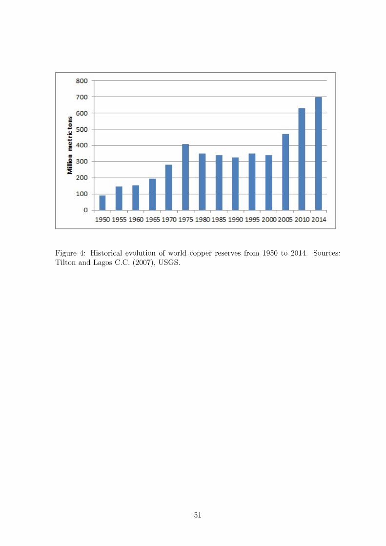
Figure 4: Historical evolution of world copper reserves from 1950 to 2014. Sources:Tilton and Lagos C.C. (2007), USGS.

51

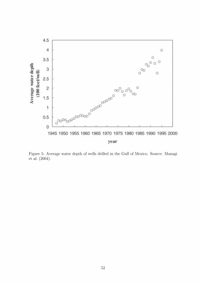
Figure 5: Average water depth of wells drilled in the Gulf of Mexico. Source: Managiet al. (2004).

52

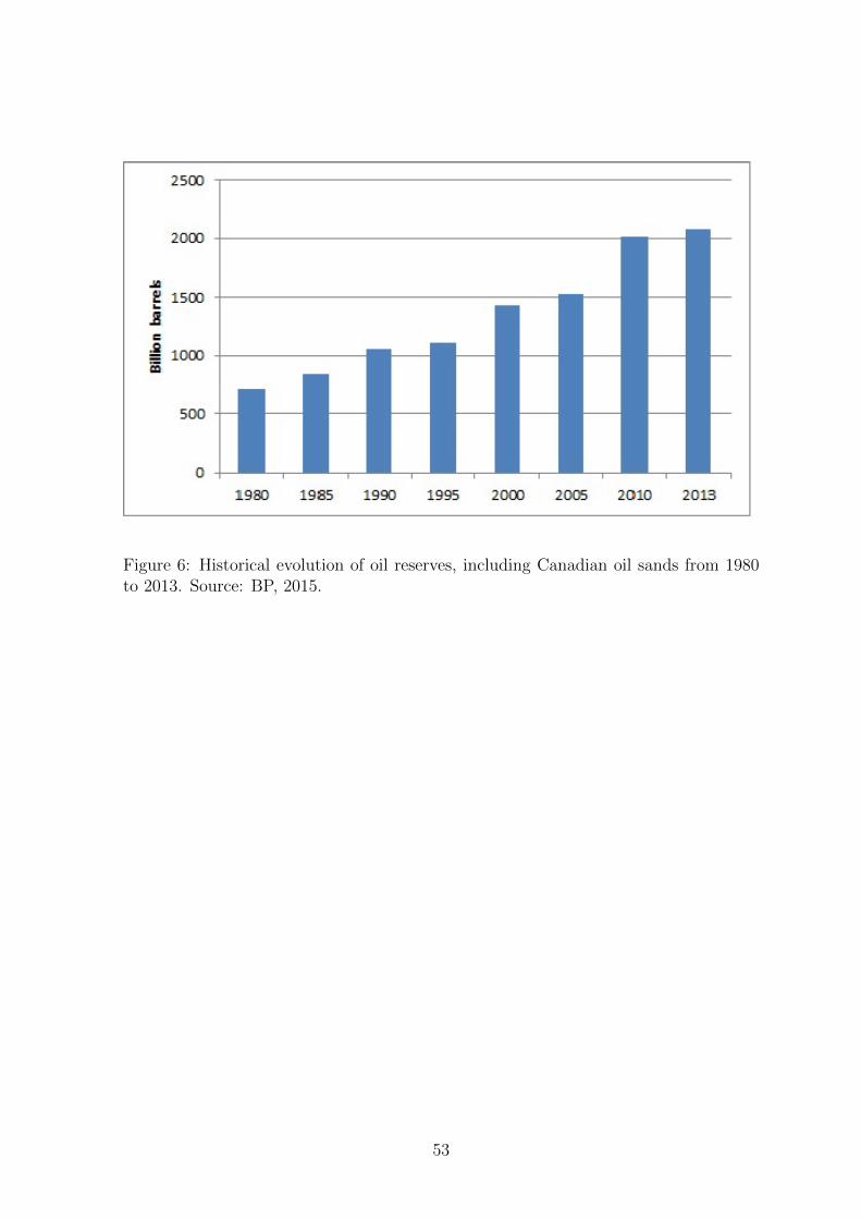
Figure 6: Historical evolution of oil reserves, including Canadian oil sands from 1980to 2013. Source: BP, 2015.

53

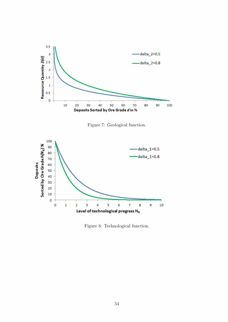
Figure 7: Geological function.

Figure 8: Technological function.

54

non-renewable resources, extraction technology, and ... · non-renewable resources, extraction...

Documents