1

Appendix#3:

Non-linear Curve fitting with Microsoft Excel Solver.1

Calculation of kobs, kreal and Debye-Hückel plot.

I. Kinetics: calculation of kobs and kreal. 1. From File click on New.., then on General Workbook:

1 Written by Dr. Mircea Gheorghiu.

2

2. From File, Save as… the workbook. My preference for file name is Kinetics_MG (MG are my initials) and it is saved in the Personal folder.

3

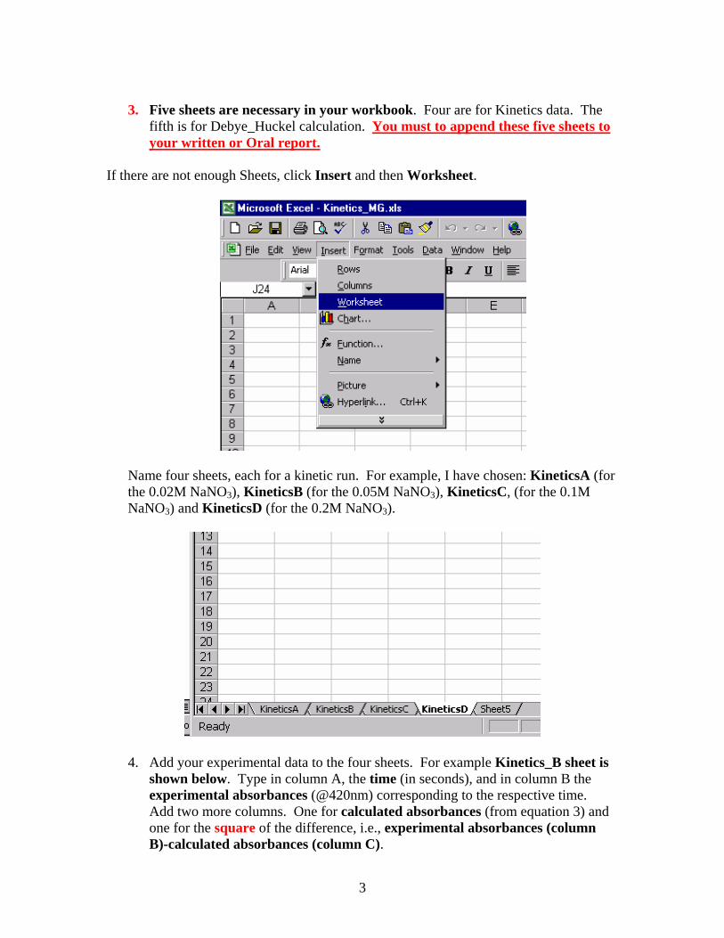
3. Five sheets are necessary in your workbook. Four are for Kinetics data. The

fifth is for Debye_Huckel calculation. You must to append these five sheets to your written or Oral report.

If there are not enough Sheets, click Insert and then Worksheet.

Name four sheets, each for a kinetic run. For example, I have chosen: KineticsA (for the 0.02M NaNO3), KineticsB (for the 0.05M NaNO3), KineticsC, (for the 0.1M NaNO3) and KineticsD (for the 0.2M NaNO3).

4. Add your experimental data to the four sheets. For example Kinetics_B sheet is shown below. Type in column A, the time (in seconds), and in column B the experimental absorbances (@420nm) corresponding to the respective time. Add two more columns. One for calculated absorbances (from equation 3) and one for the square of the difference, i.e., experimental absorbances (column B)-calculated absorbances (column C).

4

5. The second order integrated kinetic equation is given below (see the lecture hand-out):

)tkcexp(A

AA1

1AAobsf

ff

−−

−=

0

0(3)

Integrated second order kinetic equation in terms of absorbance that is curve-fitted to the experimental data.A0= initial absorbanceA = absorbance at time tAf = absorbance when all H2Asc has reacted.

6. Before using Microsoft Excel Solver cells containing two sets of information

must be added to each kinetic sheet. Cells H2 and H3 contain the values of the “fixed” variables A0 and epsilon, respectively. The content of the cells H5 (Af value) and H6 (kobs) changes. Initially, “guess” values are typed in for the variables of Af and kobs. After the minimization process, Solver returns the regression coefficients to cells H5 and H6, respectively. Solver does not provide the standard deviations of the coefficients.

5

7. In order to be automatically plug into the kinetic equation (equation 3), the cells containing the values of A0, epsilon, Af, kobs must be given a name (this is an Excel requirement). First, input the required values.

• For A0, type “=B2” in cell H2 • For epsilon type in cell H3, your value for epsilon (calculated from Lambert-Beer

equation, recorded during day #1). The slope of the least square straight line, calculated from my results, gave ε = 1020.

• Type in cell H5 the best guess value for Af, that is 0.25 (Explain why in your report).

• Type your guess value for kobs in cell H6. My guess is 5.

Next assign “Excel names” to A0, epsilon, Af and kobs. For example to name A0, first click on cell H2. Then click on Insert, Name, Define:

The following window pops-up:

6

Please check the location of the value of A0. In this example A0 is in (according to Excel grammar): KineticsB!$H$2, that is on KineticsB sheet in location H2. Click on add button. Click on OK. Continue naming cells H3:H5. Next, name as t the vector A2:A22. First highlight the column A2:A22, then click on Insert, Name, Define and change the name in the workbook as t (check the Refers to address in order be sure the correct set of cells are defined). The Define Name window will look like:

7

8. Solver optimizes the curve fitting in two steps:

• In the first step, “crude” values of absorbances are calculated. • In the second step, the optimization step, the crude values of calculated

absorbances are refined to best fit the experimental values.

A. The “Crude Calculation” Step: Type in cell C2 =Af/((1-((A0-Af)/A0)*EXP(-kobs*t*Af/epsilon))). Cell H2 is filled with the calculated absorbance for t=0 seconds. According to equation 3 it should equal A0.

To fill cells C3 through C22, click on cell C2. Bring the cursor to the right low corner and press left mouse and drag all the way down to cell C22. Depress the left mouse. All cells (C2:C22) should now be filled in with the calculated (“crude”) Absorbances:

8

B. Optimization step: Non-linear curve fitting step.

9. In cell D2 type “=(B2-C2)^2.” Press Enter key. 10. Click on cell D2. Drag all the way down to cell D22, as described for calculating

absorbances. 11. In cell D23 sum (click on icon Σ) D2 through D22.

9

Then press the Enter key.

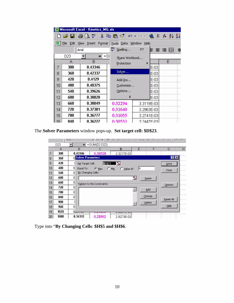
12. Click on cell D23, then click on Tools followed by Solver…

10

The Solver Parameters window pops-up. Set target cell: $D$23.

Type into “By Changing Cells: $H$5 and $H$6.

11

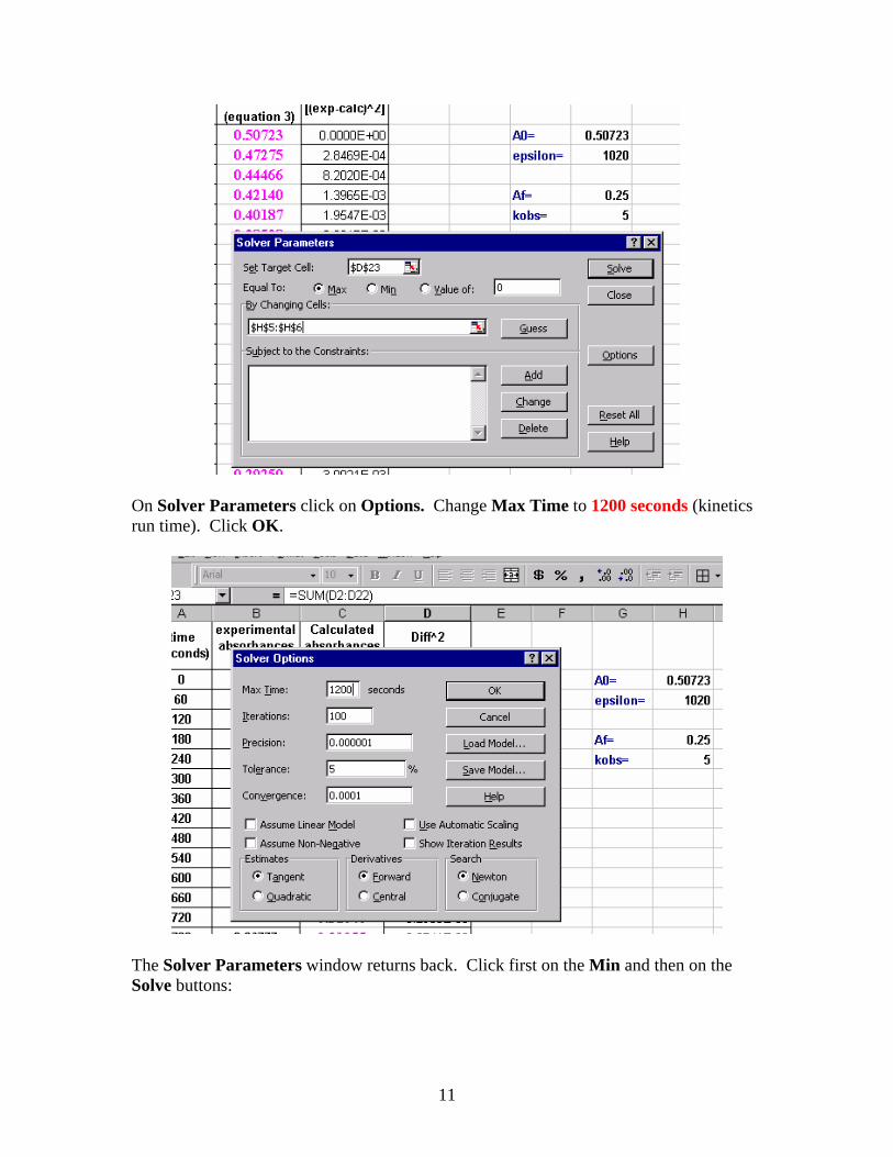
On Solver Parameters click on Options. Change Max Time to 1200 seconds (kinetics run time). Click OK.

The Solver Parameters window returns back. Click first on the Min and then on the Solve buttons:

12

The Solver Results window pops-up. Note that the values in cells H4 and H5 are updated. You know by now the value of kobs is now 2.60. (Note the initial value of kobs, the “guess,” was 5.)

You can next print reports: answer, sensitivity and limits. For example, the Answer Report looks like:

13

Repeat steps 4 through 12 for sheets KineticsA, KineticsC and KineticsD. It will be necessary to change the Reference in the Define Name window to match each sheet. II. Debye-Hückel equation. In the “Kinetics” hand-out, the Debye-Hückel equation is defined as:

21

21

021

21

210 13021

1 /

/

/

/

real II**.klog

IIZ*Z*1.02klogklog

++=

++= (6)

where kreal is given by equation (4):

[ ]1a

obsreal KHkk

+

= (4)

Use sheet#5 (named as Debye-Hückel) to compute and draw the linear plot logkreal (y axis) versus I0.5/(I0.5+1) (x axis). When finished the Debye-Hückel worksheet will look like:

14

1. Build a Table of 7 columns and 5 rows. The order and the content of the headings are suggested above. Remember in Excel x-axis values are left of y-axis values (for example, column A values are on the x-axis, column B values are displayed on the y-axis).

2. Fill in kobs values by using the address from the respective worksheet. Click, for example on cell C2 and type: “=KineticsA!$H$6”. Cell two is filled with the value 2.07. Cell C3: “=KineticsB!$H$6”, cell C4: “=KineticsC!$H$6” and cell C5: “=KineticsD!$H$6”.

15

3. Place the HNO3 molarity in cell B7 and the acidity constant for ascorbic acid (Ka1=6.76*10-5) in cell B8.

4. Type in the column D2 through D5 the calculated kreal (see equation 4). For

example in cell D2 type: “=(C2/$B$8)*0.5*$B$7” (the 0.5 appears because the HNO3 in the UV cuvette is half the concentration of the HNO3 stock solution). Because cells B7 and B8 are referred to by absolute address, for example $B$7, you can generate automatically the content of the subsequent D2:D5 cells. Click on D2, move the cursor to right lower corner and pressing left mouse, drag all the way down to D5. Cells are filled automatically.

16

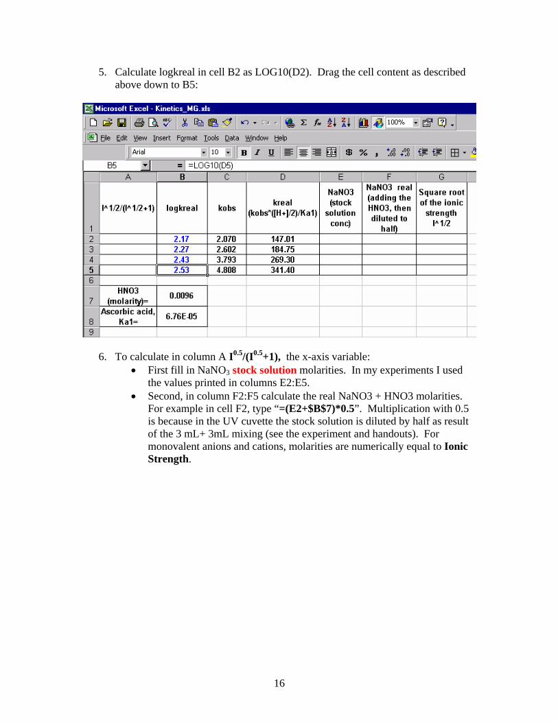
5. Calculate logkreal in cell B2 as LOG10(D2). Drag the cell content as described above down to B5:

6. To calculate in column A I0.5/(I0.5+1), the x-axis variable: • First fill in NaNO3 stock solution molarities. In my experiments I used

the values printed in columns E2:E5. • Second, in column F2:F5 calculate the real NaNO3 + HNO3 molarities.

For example in cell F2, type “=(E2+$B$7)*0.5”. Multiplication with 0.5 is because in the UV cuvette the stock solution is diluted by half as result of the 3 mL+ 3mL mixing (see the experiment and handouts). For monovalent anions and cations, molarities are numerically equal to Ionic Strength.

17

• Third, in cells G2:G5 calculate the square root of value from cell F2:F5. For example, in cell G2 type “=SQRT(F2)” and press Enter.

• Fourth, in cells A2:A5 calculate I0.5/(I0.5+1). For example, in cell A2 type “=G2/(G2+1)” and press Enter. Click on the cell. Drag the lower right corner all the way down to A5.

7. The last step consists of the Debye-Hückel plot. • Highlight columns A2:B5. Click on Insert, then Chart…:

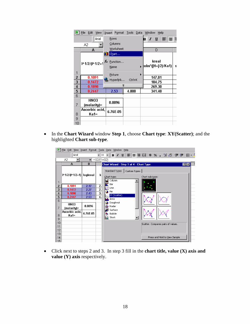
18

• In the Chart Wizard window Step 1, choose Chart type: XY(Scatter); and the highlighted Chart sub-type.

• Click next to steps 2 and 3. In step 3 fill in the chart title, value (X) axis and value (Y) axis respectively.

19

• Click Next and then Finish. • With some editing, the chart appears as:

• The least square straight line is added on the graph, by clicking on Chart, then Add trendline..

20

Under Type: Trend/Regression type, choose Linear.

• Click on Options. Check Display equation on the chart and Display R-squared value on the chart:

21

• The least square straight line below has the equation: y = 2.7835x + 1.8686 and R2=0.9809 (satisfactory, however I am confident that 5.310 students will get a better R2).

8. To compute the slope (1.02*Z1*Z2) and intercept ( ko the rate constant at I=0), and R2, first add these cells (A10:A13; B10:B13) to the Debye-Hückel worksheet.

• Type” =SLOPE(B2:B5,A2:A5)” in cell B10, next to Slope=. • Type “= INTERCEPT(B2:B5,A2:A5)” in cell B11, next to Intercept= • Type “=10^B11” in cell B12, next to k0=

22

• Type “=RSQ(B2:B5,A2:A5)” in cell B13, next to R^2=

9. Finally print copies of all 5 sheets for inclusion with your report.