non-euclidean geometryfaculty.mansfield.edu/hiseri/old courses/sp2013/ma3330... · 2013-01-28 ·...

CHAPTER 5

Non-Euclidean Geometry

1. A model for hyperbolic geometry

When you build an axiom system for something like Euclidean geometry,

you try to gather a basic set of statements that, if assumed to be true, define the

object you’re trying to axiomatize. In the case of Euclidean geometry, one such axiom

system is Hilbert’s. The hope is that if you take the set of theorems you can prove

from Hilbert’s axioms, they are exactly the same as the theorems you would expect

to be true in your vision of Euclidean geometry.

Beyond the issue of getting the correct set of theorems, there are three things you

look for in an axiom system, consistency, independence, and completeness. An axiom

system is consistent, if it does not lead to contradictions. If, in your axiom system,

you could prove that the angle sum of a triangle is always 180◦, and you could also

prove that the angle sum is sometimes not 180◦, then your axiom system would not

be consistent.

An axiom system is independent, if you cannot prove any of your axioms from

the others. In the attempt to prove Euclid’s Fifth Postulate from the other axioms,

the underlying suspicion was that Euclid’s axiom system was not independent. With

independence, we are wanting to ensure that our set of axioms is minimal, and that

every axiom is actually needed.

Finally, an axiom system is complete, if we cannot add another axiom without

losing consistency or independence. Hilbert’s axiom system has been shown to be

incomplete several times since it’s original formulation, and additional axioms were

introduced to fix the various problems. We probably will never be absolutely sure

about the completeness of this axiom system, but it seems like the general assumption

is that Hilbert’s axiom system is complete.

None of these things is easy to prove, but the most important and easiest to

verify is consistency (note the use of verify, since prove would be too strong). In this

86

2. THE POINCARE DISK 87

assignment, we wish to investigate how the axioms of hyperbolic geometry can be

shown to be consistent, and at the same time, determine that the neutral geometry

axiom set is not complete.

1.1. Exercises.

–1– State Euclid’s Axiom.

–2– State the Hyperbolic Axiom.

–3– If you had both Euclid’s Axiom and the Hyperbolic Axiom in the same axiom

system, would that axiom system be consistent?

–4– Assuming that neutral geometry plus Euclid’s Axiom and neutral geometry

plus the Hyperbolic Axiom are both consistent, can neutral geometry be

complete?

–5– From what we’ve been exploring the last couple of weeks, neutral geometry

plus Euclid’s Axiom plus angle sum of a triangle is 180◦ would definitely not

be (consistent, independent, complete).

2. The Poincare Disk

We can test the consistency of hyperbolic geometry by comparing it to some-

thing that we have confidence in. The mathematics we work with today is built on

axioms systems for logic and set theory. I don’t want to get into it too much,

but logic and set theory are simpler than geometry, and their axioms systems were

formulated to be axiom systems (Euclid was not an expert in axioms systems). As

a result, we can be more confident in these modern systems. I have great confidence

in these axiom systems, but it is only confidence. Mathematicians like to think that

mathematics is absolute truth, but at best, we only have faith in our understanding

of logic. Mathematics is not a religion exactly, but at its foundations, we believe in

mathematics with fanatical conviction.

If we can build a mathematical object, a model, within our modern mathematical

structure, and the axioms of hyperbolic geometry are true for our model, then we

can say that hyperbolic geometry, as an axiom system, is as consistent as the rest

of mathematics. That’s what we want to do here. The xy-plane is a model for

Euclidean geometry, and we saw that Euclid’s postulates, and therefore, some of


Hilbert’s axioms, were true in that model. I think it’s safe to assume that all of

Hilbert’s axioms are true in our xy-plane model for Euclidean geometry.

The model for hyperbolic geometry to be discussed in this assignment is called

the Poincare disk. Poincare’s model lives in the xy-plane (a.k.a, R2), and consists

of all of the points inside a fixed circle. For convenience, let’s nail down the circle.

The points in this geometry are the points in the set P defined by

(163) P ={

(x, y) ∈ R2 | x2 + y2 < 1}

.

In words, P is the set of points inside the unit circle, but not including the circle itself.

We might call this an open disk. The lines in this geometry are parts of circles. In

particular, we will consider any circle that intersects the unit circle at right angles.

The intersection of any such circle and P will be a line. It is convenient to think of

a straight line as a circle with infinite radius, and we will do that. Diameters of the

unit circle, therefore, are also lines (not including the endpoints). Figure 1 shows a

few lines in the Poincare Disk. Viewed in terms of the xy-plane, these are straight

lines or circles that meet the boundary at right angles.

Figure 1. Some lines in the Poincare Disk.

Note that near the center of Figure 1 there is a small triangle. Since one of the

edges of this triangle is curved slightly inward, two of the angles are slightly smaller

than they would be if that edge were straight. Since the straight lines only pass

through the center of the disk, we will never have a triangle with three straight sides.

We will measure angles in this geometry as we see them (technically, we measure the

angles between tangent lines).


Basic Principle 4. Since the sides of triangles in the Poincare disk curve in-

ward, their angle sums will be less than 180◦.

There is a horizontal diameter and a quarter circle in the lower left that intersect

on the unit circle on the left. Since the unit circle is not part of P, these two lines

do not intersect. Since according to Euclid’s definition of parallel lines (and ours),

parallel lines are those pairs that do not intersect. Therefore, these two lines are

parallel.

Figure 2. The lines m and n contain P and are parallel to l.

In Figure 2, the lines m and n intersect l at the boundary, so in the model, they

do not actually intersect. Both lines, therefore, are parallel to l. This model satisfies

the Hyperbolic Axiom (there are at least two parallels through P ).

If you were to consider all of the lines through P in Figure 2 some are parallel to

l and some intersect. Imagine taking a single line t through P and rotating it about

P . You will find that t intersects l for awhile, and then it will be parallel. A little

later, it will start intersecting again. During the change, there will be one position

such that everything before is not parallel and everything after is parallel. At this

position itself, is t parallel or does it intersect l? It has to be parallel, because if

not, then there would be a point of intersection. If this happens, then there would

be other points of intersection on either side of it on l, and therefore, there would

be non-parallels on either side of it. In hyperbolic geometry, therefore, we have the

phenomenon of a last parallel.

3. DISTANCE IN THE POINCARE MODEL 90

3. Distance in the Poincare model

One important aspect of this model must be different from how it looks. In

hyperbolic geometry, lines must be infinitely long. In order to satisfy the axioms of

hyperbolic geometry, therefore, we must define distances in a funny way. I won’t give

you the general formula for the distance between any two points (this formula would

be called the metric). I’ll just tell you what the distance between any point and the

point in the center of the model. For any point P ∈ P, if the distance from the center

is r, as we would measure it in the xy-plane, then the hyperbolic distance will be

(164) d(0, r) = ln

(1 + r

1 − r

).

As a point is moved towards the boundary, r would approach 1. Its hyperbolic

distance from the center would therefore approach

(165) limr→1

d(0, r) = limr→1

ln

(1 + r

1 − r

)= ∞.

The hyperbolic distance from the center out to the boundary, therefore, must be

infinite.

3.1. Exercises.

–1– Suppose you were 2-dimensional, and the Poincare disk was your universe.

Suppose also that when you stood on the x-axis at the center, the top of

your head would be at the point (0, 0.1). What is your height in hu’s (hu =

hyperbolic unit)?

–2– If my height were 0.3 hu’s, and I stood on point (0, 0.8) with my head pointing

up the y-axis, I could figure out where my head was. My feet would be

5. IS HYPERBOLIC GEOMETRY REAL? 91

ln(

1.8.2

)= 2.197 hu. My head would be at ln

(1+r1−r

)hu. Therefore,

.3 = ln

(1 + r

1 − r

)− 2.197

2.497 = ln

(1 + r

1 − r

)

e2.497 =1 + r

1 − r

(1 − r)e2.497 = 1 + r

e2.497 − 1 = r + re2.497

e2.497−1 = r(1 + e2.497)

e2.497 − 1

1 + e2.497= r

(166)

Therefore, r = 0.848, and my head would be at (0, 0.848). If you were

standing on the point (0, 0.9) with your head pointing up the y-axis, where

would your head be?

4. What does the Poincare disk tell us?

With the definitions I’ve given you, and a few more, you could show that all the

axioms of neutral geometry are true in this model, and in addition, the Hyperbolic

Axiom is true in this model. It might take you awhile, but you could show that all

of the definitions are well-defined (i.e., don’t give contradictory answers). This would

mean that the Poincare disk is consistent within our modern mathematical system,

and this would imply that the axioms of hyperbolic geometry are as consistent as the

axioms for logic and set theory. In other words, if the axioms of hyperbolic geometry

are bad, then all of mathematics is in trouble. That might be interesting, actually.

As far as independence and completeness are concerned, the axioms of hyperbolic

geometry are probably both independent and complete. I’m not an expert on such

matters, but I don’t think either has been proven.

5. Is hyperbolic geometry real?

Most of us seem to be comfortable with the assumption that our universe is a

3-dimensional Euclidean space, the xyz-space of calculus. In fact, Bertrand Russell

5. IS HYPERBOLIC GEOMETRY REAL? 92

filled a small book, I think it’s called An Essay on the Foundations of Geometry,

“proving” that this was indeed the case. This essay was written around 1900. About

30 years later, Russell states as fact that our universe is a manifold. We’ll get to

manifolds later, but most manifolds are definitely not Euclidean. I’m working from

memory here, but I think the second reference is in something called Principles of

Mathematics. I’m been trying to track these down for awhile.

Now, the Poincare disk lives in the Euclidean plane, so it definitely seems sub-

ordinate to Euclidean geometry. We could, perhaps, put it on more equal footing

by stretching it out so that distances could be measured directly. Since things get

smaller towards the boundary, we would have to stretch the Poincare’s disk more and

more as we move away from the center. If we did this, we would get something called

the hyperbolic plane, and this plane will stretch out to infinity.

What would the hyperbolic plane look like? Well, if you took a small piece

of the Poincare disk, and did the stretching, you would get something that looked

like the picture on page 133 of Bonola’s Non-Euclidean Geometry. Notice that it is

really wrinkly. This is because hyperbolic geometry spreads out faster than Euclidean

geometry spreads out. For example, a circle in hyperbolic geometry has a larger

circumference than a circle in Euclidean geometry with the same radius. So in some

sense, the hyperbolic plane is too big to fit in our supposedly Euclidean space, so it

has to be crammed into our space, and it gets wrinkled in the process. This is not

proof that our space is Euclidean, however. Later, we will describe how hyperbolic

a space is in terms of curvature. We’ll say that the hyperbolic plane has curvature

K = −1. A hyperbolic plane with curvature K = −.003 might look perfectly flat in

our space, because if our universe is hyperbolic, it would have very small curvature.

We’ll spend much of the rest of the semester trying to understand these ideas, but

let me end with this. We have direct experience with the geometry of our universe

only on the surface of the earth, and the visible universe has a radius of only 10-

15 billion light-years. There are an infinite number of distinctly different geometric

spaces consistent with the information we have. One of the problems I have with

Hilbert’s axioms is that they lead to only two of these spaces.

6. ANOTHER MODEL FOR HYPERBOLIC GEOMETRY 93

6. Another model for hyperbolic geometry

Before we move on to a more contemporary view of geometry, I want to finish off

this line of geometric reasoning. So far, we have seen that Euclid came up with a set of

definitions and postulates for what we call Euclidean geometry. Much later, Hilbert

formalized Euclid’s system into a somewhat modern axiom system using Euclid’s

approach as much as possible. For convenience, let’s pretend that Euclid’s system

of postulates and Hilbert’s axiom system are the same, since Hilbert’s work can be

thought of as patching up Euclid’s original attempt.

Until the time of Gauss, Lobachevski, and Bolyai, the general assumption was

that Euclid’s axiom system was not independent. In particular, it was conjectured

that Euclid’s Fifth Postulate/Euclid’s Axiom could be proven from the other axioms.

Gauss, Lobachevski, and Bolyai realized that this was impossible. In fact, there was

another geometry, hyperbolic geometry, that satisfied all of the “other” axioms,

but not Euclid’s Fifth Postulate. This marked the beginning of what is generally

called non-Euclidean geometry. Hyperbolic geometry, after all, is a geometry

that is not Euclidean.

Somewhat oddly, non-Euclidean geometry doesn’t refer to all geometries that

are not Euclidean, but for the most part, only refers to hyperbolic geometry and

something called elliptic geometry. We’ll talk about elliptic geometry later, but

it is very similar to, or exactly the same as (depending on who you’re talking to),

spherical geometry.

As I’ve said before, hyperbolic geometry is sometimes referred to as the geometry

of Lobachevski and/or Bolyai, although Gauss, Cayley, and Klein are important in

its development. The other non-Euclidean geometry, elliptic geometry, is sometimes

referred to as the geometry of Riemann. The names hyperbolic and elliptic are

due to Felix Klein. The study of geometry through axiom systems like Hilbert’s is

called synthetic geometry, and this line of geometric reasoning pretty much comes

to a dead end at the geometries of Euclid, Lobachevski/Bolyai, and Riemann. The

study of geometry through coordinates, equations, and functions is called analytic

geometry, and we will start to head in that direction today.

7. THE HALF-PLANE MODEL FOR HYPERBOLIC GEOMETRY 94

7. The Half-Plane Model for Hyperbolic Geometry

As much as you can, try to think of the hyperbolic plane as an infinite plane

that is no more or less real than the Euclidean plane (i.e., the xy-plane). Our brains

have a very strong Euclidean bias. Try to suppress this geometricism. Because of

this geometrism, it is difficult to visualize the hyperbolic plane, but by deforming the

hyperbolic plane, we can squeeze it into our familiar Euclidean plane as an open disk,

the Poincare disk. This is only one way of visualizing the hyperbolic plane, and I

want to explore another way here.

The set of points in the half-plane model is the set

(167) HP ={

(x, y) ∈ R2 | y > 0}

.

These are all the points above the x-axis, but not including the x-axis itself. In other

words, we have an open upper-half-plane. As we deform the hyperbolic plane into

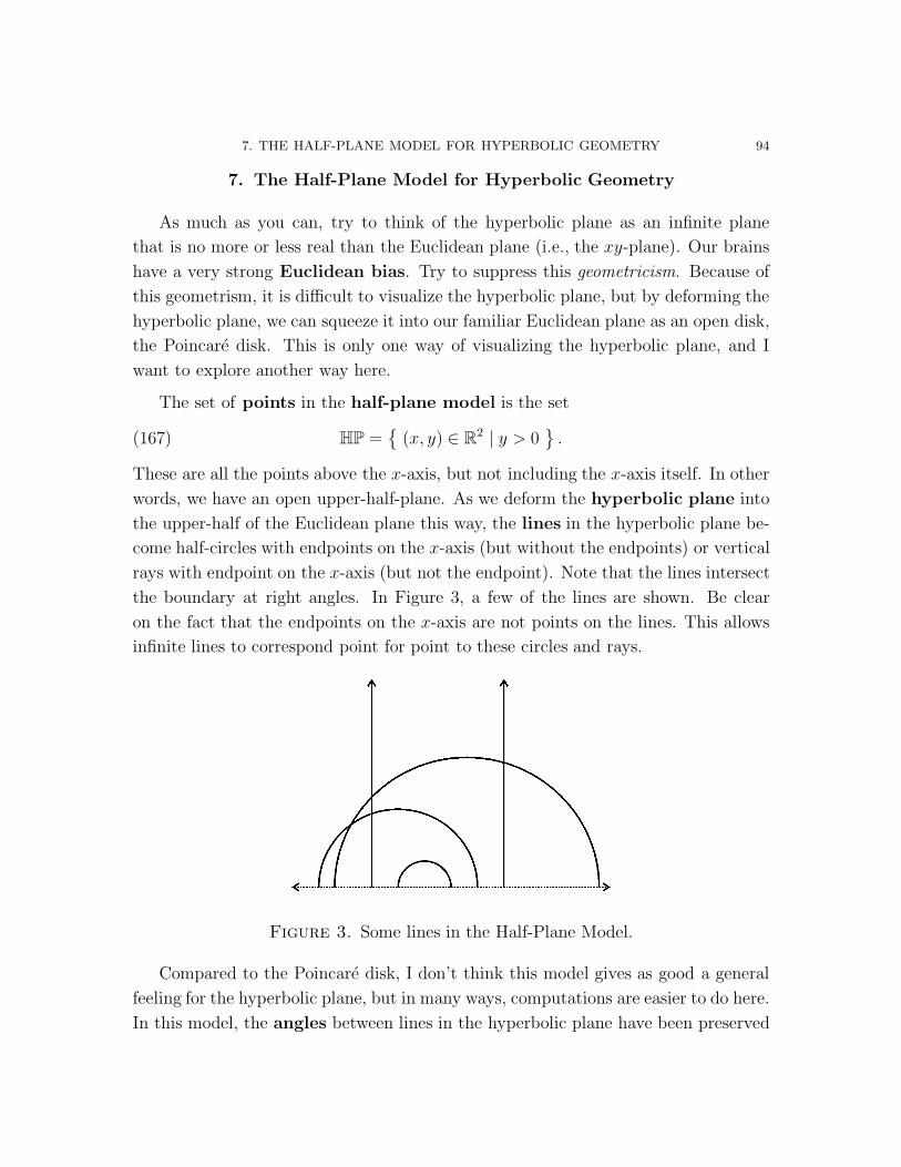
the upper-half of the Euclidean plane this way, the lines in the hyperbolic plane be-

come half-circles with endpoints on the x-axis (but without the endpoints) or vertical

rays with endpoint on the x-axis (but not the endpoint). Note that the lines intersect

the boundary at right angles. In Figure 3, a few of the lines are shown. Be clear

on the fact that the endpoints on the x-axis are not points on the lines. This allows

infinite lines to correspond point for point to these circles and rays.

Figure 3. Some lines in the Half-Plane Model.

Compared to the Poincare disk, I don’t think this model gives as good a general

feeling for the hyperbolic plane, but in many ways, computations are easier to do here.

In this model, the angles between lines in the hyperbolic plane have been preserved


under the deformation. That is, the angles we see are the same as the actual angles.

The distances have been warped, however. They have been changed by a factor of

y, where y is the height above the x-axis. When we transform back to the hyperbolic

plane, therefore, we have to divide distances by y.

ϕ

2

Figure 4. An arc of the circle of radius 2. This would correspond to

a hyperbolic line segment in the hyperbolic plane.

As an example, consider the half-circle of radius 2 in Figure 4. In the Euclidean

plane, the circumference of the entire circle is 2π(2) = 4π. Since there are 2π radians

around the circle, the length of the arc s divided by C must be equal to ϕ2π

. Therefore,

(168) s = 2ϕ.

If ϕ = π6

radians, for example, then s = π3. This is only the length of the segment

as we see it in the Euclidean plane. We want to know the hyperbolic length. The

highest point on the arc is at height y = 2, and the rest of the arc is not too much

lower. We can say, therefore, that the height is approximately y = 2 for the entire

arc. To get an approximation of the length of the corresponding hyperbolic segment,

we need to divide the length of the arc by y = 2, so the hyperbolic length is about π6.

This is only an estimate, however, since the height of the points on the arc are not

all exactly y = 2.

7.1. Computation of hyperbolic length. As we move along a circle, the con-

version factor to hyperbolic length keeps changing. In order to do the conversion,

therefore, we need to do an integration. File this away in your brain: In general, the

conversion between geometries is a calculus problem.


θ

dθ

ds

r

r sin θ

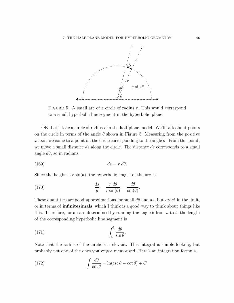
Figure 5. A small arc of a circle of radius r. This would correspond

to a small hyperbolic line segment in the hyperbolic plane.

OK. Let’s take a circle of radius r in the half-plane model. We’ll talk about points

on the circle in terms of the angle θ shown in Figure 5. Measuring from the positive

x-axis, we come to a point on the circle corresponding to the angle θ. From this point,

we move a small distance ds along the circle. The distance ds corresponds to a small

angle dθ, so in radians,

(169) ds = r dθ.

Since the height is r sin(θ), the hyperbolic length of the arc is

(170)ds

y=

r dθ

r sin(θ)=

dθ

sin(θ).

These quantities are good approximations for small dθ and ds, but exact in the limit,

or in terms of infinitesimals, which I think is a good way to think about things like

this. Therefore, for an arc determined by running the angle θ from a to b, the length

of the corresponding hyperbolic line segment is

(171)

∫ b

a

dθ

sin θ.

Note that the radius of the circle is irrelevant. This integral is simple looking, but

probably not one of the ones you’ve got memorized. Here’s an integration formula,

(172)

∫dθ

sin θ= ln(csc θ − cot θ) + C.

8. COMPUTING AREA IN THE HYPERBOLIC PLANE 97

For the arc above, we would have

(173)

∫ 7π/12

5π/12

dθ

sin θ= ln(csc θ − cot θ)

∣∣∣∣7π/12

5π/12

= 0.52968449 . . .

Compare this to π6

= 0.52359877 . . ., which was the approximation we got before.

dxdy

y

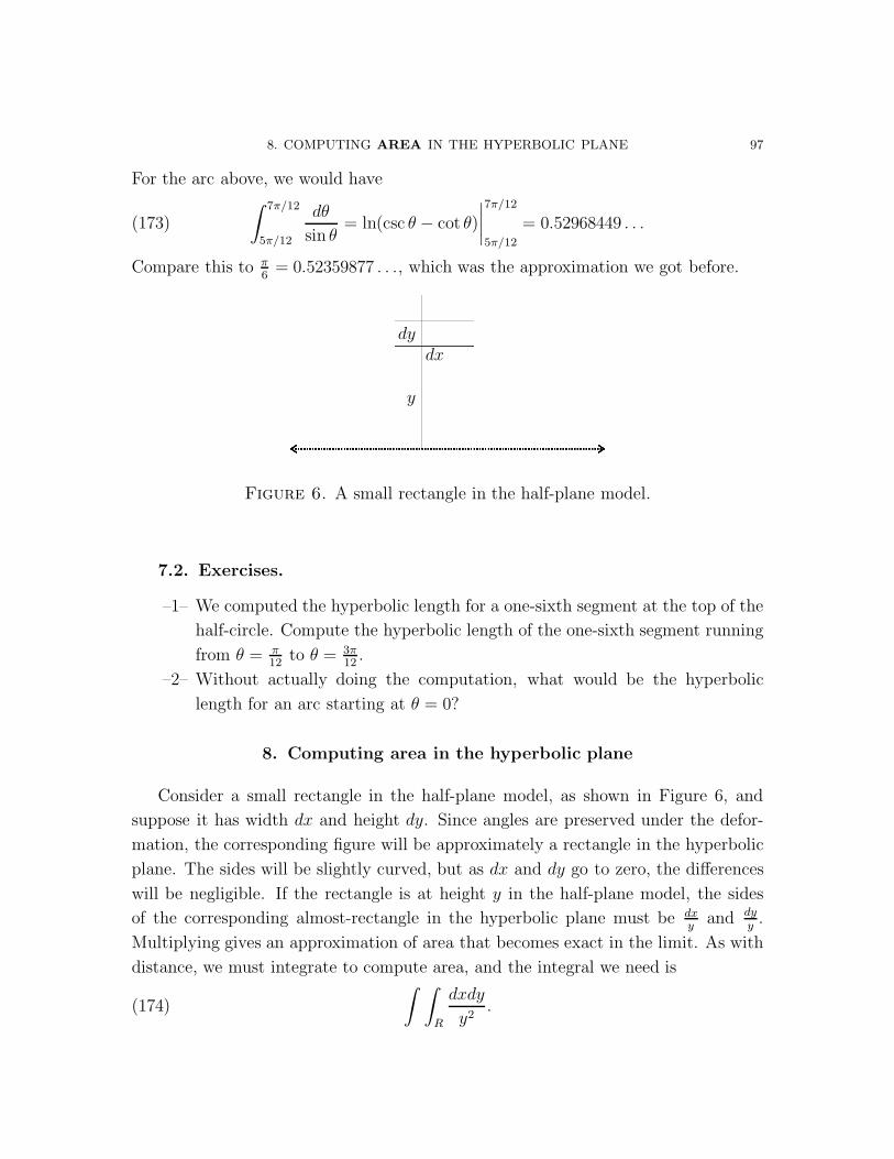
Figure 6. A small rectangle in the half-plane model.

7.2. Exercises.

–1– We computed the hyperbolic length for a one-sixth segment at the top of the

half-circle. Compute the hyperbolic length of the one-sixth segment running

from θ = π12

to θ = 3π12

.

–2– Without actually doing the computation, what would be the hyperbolic

length for an arc starting at θ = 0?

8. Computing area in the hyperbolic plane

Consider a small rectangle in the half-plane model, as shown in Figure 6, and

suppose it has width dx and height dy. Since angles are preserved under the defor-

mation, the corresponding figure will be approximately a rectangle in the hyperbolic

plane. The sides will be slightly curved, but as dx and dy go to zero, the differences

will be negligible. If the rectangle is at height y in the half-plane model, the sides

of the corresponding almost-rectangle in the hyperbolic plane must be dxy

and dyy.

Multiplying gives an approximation of area that becomes exact in the limit. As with

distance, we must integrate to compute area, and the integral we need is

(174)

∫ ∫

R

dxdy

y2.


r

θ

θ

θ

l m

n

inside

Figure 7. A doubly asymptotic triangle.

In Figure 7, we have three hyperbolic lines. One is represented by the half-circle,

and the other two by vertical lines.

The lines m and n intersect forming vertical angles measuring θ. The lines l and

n only intersect at the boundary, so they’re actually parallel in the hyperbolic plane.

The lines l and m are parallel as we see them lying in the half-plane model, and

since they do not intersect, they are also parallel as lines in the hyperbolic plane. In

the model, the distance between the two lines l and m is r + r cos θ. We’re used to

thinking of parallel lines as being a fixed distance apart all along them. That’s not

true in the hyperbolic plane. As we measure the horizontal distance between l and m,

the corresponding hyperbolic distance is obtained by dividing by the height y. That

is, the distance between the lines is

(175)r + cos θ

y,

and this distance goes to zero, as y goes to ∞. As you can see, it’s possible for two

parallel lines to approach each other asymptotically. This happens with l and n, as

well. This is one of the odd things that can happen in the hyperbolic plane. On the

other hand, maybe this isn’t so odd. Have you ever followed a pair of parallel lines

out to infinity? I haven’t.

Since the “upper ends” of l and m are as close as they can get without intersecting,

if we looked at them in the Poincare Disk, they would “intersect” on the boundary.

In fact, the pair l and m and the pair l and n look exactly the same in the hyperbolic

plane. We could even rotate the figure a bit to make these three lines look like Figure


θ

θ

l

m

n

inside

Figure 8. Exactly the same doubly asymptotic triangle as in Figure

7, but rotated a bit.

8. Looking at Figure 8, I’ve positioned the word inside to indicate a triangular region

with curved edges. These edges are straight, however, in the hyperbolic plane, so it

makes sense to call this a triangle. On the other hand, two of the vertices are “at

infinity,” so we’ll call this a doubly asymptotic triangle. The doubly refers to the

two asymptotic vertices. The “ends” of the half-circles meet the boundary at right

angles, so the angle between l and m must be zero (assuming it makes sense to have

a vertex at infinity). The angle between l and n must also be zero. This gives us an

angle sum for this triange of

(176) 0 + 0 + θ = θ.

Hopefully, you answered the last question, zero. Now let us redirect our attention

to Figure 7. This doesn’t look like a triangle, but it’s easier to compute its area, and

we’ll see that the area is very important.

The interior of the triangle lies above the circle of radius r. For convenience, we’ll

assume the circle is centered at the origin. This doesn’t matter, since the x-axis in

this model, is exactly the same as the boundary circle in the Poincare Disk. The

origin can go anywhere.

The equation of the circle is y =√

r2 − x2. The equation of the line l is x = −r,

and the equation of the line m is x = r cos θ. (Don’t forget that r and θ are constants.)

The area of the doubly asymptotic triangle in Figure 7, therefore, is

(177) area =

∫ r cos θ

−r

∫ ∞

√r2−x2

dydx

y2.


Here’s the mess, but it’s important.

area =

∫ r cos θ

−r

∫ ∞

√r2−x2

dydx

y2=

∫ r cos θ

−r

∫ ∞

√r2−x2

y−2 dydx

=

∫ r cos θ

−r

y−1

−1

∣∣∣∞√

r2−x2dx =

∫ r cos θ

−r

−1

y

∣∣∣∞√

r2−x2dx

=

∫ r cos θ

−r

1√r2 − x2

dx = − arccos(x

r

) ∣∣∣r cos θ

−r

= − arccos(cos θ) + arccos(−1)

= −θ + π

(178)

It’s downhill from here.

Note that the r was irrelevant. The important constant is the angle θ. We can

control this by moving the line m to the left or right. As we move the line m towards

x = r on the right, the values for θ tend towards zero, and the area increases. In fact,

the area tends towards

(179) area = −0 + π = π.

The triply asymptotic triangle at the limit has area π.

If m is the line x = 0, right in the middle, θ = π2. The area in this case is

(180) area = −π

2− π =

π

2.

On the other end, as we move m towards x = −r, θ tends towards π (a straight

angle). The area appears to go to zero, and this agrees with our area formula

(181) area = −π + π.

In any case, we have the following relationships for the areas of asymptotic trian-

gles.

Lemma 1. In hyperbolic geometry, a doubly asymptotic triangle has area π − α,

where α is the measure of the non-asymptotic angle.

Lemma 2. In hyperbolic geometry, a triply asymptotic triangle has area π.

9. AREA AND THE ANGLE SUM OF A TRIANGLE 101

9. Area and the angle sum of a triangle

The angle sum of a triangle is closely tied to Euclid’s Fifth Postulate/Euclid’s

Axiom. It’s important here as well, and in fact, it can be used to unify geometry as

we know it. Conquering the inhabited regions of geometry will come later. Now we’ll

invade the plains of hyperbolic geometry. Sorry. Let’s move on.

A

B

C

D

E

F

GH

I

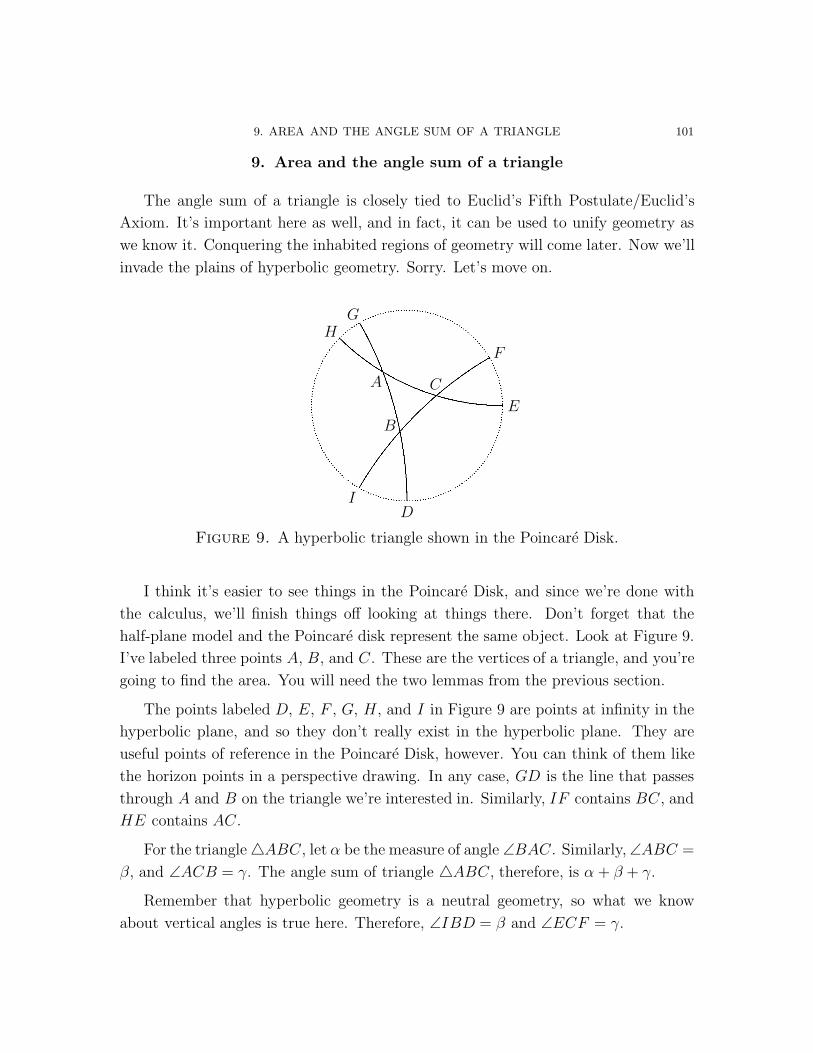
Figure 9. A hyperbolic triangle shown in the Poincare Disk.

I think it’s easier to see things in the Poincare Disk, and since we’re done with

the calculus, we’ll finish things off looking at things there. Don’t forget that the

half-plane model and the Poincare disk represent the same object. Look at Figure 9.

I’ve labeled three points A, B, and C. These are the vertices of a triangle, and you’re

going to find the area. You will need the two lemmas from the previous section.

The points labeled D, E, F , G, H, and I in Figure 9 are points at infinity in the

hyperbolic plane, and so they don’t really exist in the hyperbolic plane. They are

useful points of reference in the Poincare Disk, however. You can think of them like

the horizon points in a perspective drawing. In any case, GD is the line that passes

through A and B on the triangle we’re interested in. Similarly, IF contains BC, and

HE contains AC.

For the triangle 4ABC, let α be the measure of angle ∠BAC. Similarly, ∠ABC =

β, and ∠ACB = γ. The angle sum of triangle 4ABC, therefore, is α + β + γ.

Remember that hyperbolic geometry is a neutral geometry, so what we know

about vertical angles is true here. Therefore, ∠IBD = β and ∠ECF = γ.

9. AREA AND THE ANGLE SUM OF A TRIANGLE 102

So far, we know how to compute the areas of doubly and triply asymptotic trian-

gles, but we’re really interested in triangles that are not asymptotic at all, like our

triangle 4ABC. In order to use what we know, we need to introduce some asymptotic

triangles. One way to do this is shown in Figure 10.

A

B

C

D

E

F

GH

I

Figure 10. Some additional lines are added to Figure 9 form asymp-

totic triangles.

In Figure 10, 4ADE is a doubly asymptotic triangle. Therefore, its area is π−α.

Similarly, the area of the doubly asymptotic triangle ∆CHI is π − γ.

The area of doubly asymptotic triangle 4BID is π − β.

Looking closely at Figure 10, there is a quadruply asymptotic quadrilateral HEDI.

The area inside this quadrilateral is covered by the three areas of triangles 4ADE,

4CHI, and 4BID, except that triangle ∆ABC has been covered twice. If we knew

the area of quadrilateral HEDI, we’d have enough information to compute the area

of ∆ABC.

I’ve added one more line in Figure 11, and it divides quadrilateral HEDI into two

triply asymptotic triangles, each of which we know have area π. The area of HEDI

must be 2π.

OK. Our areas are related as follows.

HEDI = 4ADE + 4CHI + 4BID −4ABC(182)

2π = (π − α) + (π − γ) + (π − β)−4ABC.(183)

Therefore,

(184) 4ABC = π − (α + β + γ).

10. CONCLUSIONS 103

A

B

C

D

E

F

GH

I

Figure 11. With the new line IE, you can compute the area of quadri-

lateral HEDI.

We’ve just proved a really really important theorem in hyperbolic geometry.

Theorem 9. In hyperbolic geometry, if a triangle has angles α, β, and γ measured

in radians, then

(185) α + β + γ = π − area.

In other words, the angle sum of a triangle in hyperbolic geometry is π minus the area

of the triangle.

10. Conclusions

In hyperbolic geometry, the angle sum of a triangle is always less than 180◦. The

difference between the angle sum and 180◦ is called the triangle’s angle sum defect

or angle sum deficit. Expressed in radians, the angle sum defect is always equal to

the triangle’s area.

Since hyperbolic geometry is a neutral geometry, we can now see why it was

impossible to prove that the angle sum of a triangle is 180◦. Basically, because it’s

not necessarily true.

10.1. Exercises.

–1– Suppose I have a hyperbolic triangle and two of its angles measure π3

radians.

If the area of the triangle is π4, what is the measure of the third angle?

11. A MODEL FOR SPHERICAL/ELLIPTIC GEOMETRY 104

–2– Express Theorem 9 in degrees.

11. A model for spherical/elliptic geometry

In a typical modern geometry course, you would have finished about where we

are now, although you would have looked at Hilbert’s axiom system in a lot more

detail, of course. You might also have seen spherical geometry or elliptic geom-

etry at the end. Before we complete this part of the course with spherical/elliptic

geometry, let me give an overview of what we know.

Hilbert’s axiom system goes with Euclidean geometry. This is the same geometry

as the geometry of the xy-plane. Mathematicians have come to view Hilbert’s axioms

as a bunch of very obvious axioms plus one special one, Euclid’s Axiom. The special-

ness of Euclid’s Axiom is partly historical, but there are good mathematical reasons,

as well.

Euclid’s Axiom. Given a line l and a point P not on l, there is at most one

line through P that is parallel to l. (We could have said exactly one line parallel here)

Euclid’s Axiom in the context of neutral geometry is equivalent to the statement,

“The angle sum of a triangle is 180◦.” We’re going to embrace this alternative as

we move on. We can draw a picture of a triangle, but we can’t draw parallel lines

(showing the entire length of the lines). With parallel lines, the important stuff

happens (or doesn’t happen) outside of the picture, and we’ve kind of started to see

that what happens outside of the picture is not as obvious as we think. We’ll see this

more and more.

One big transition in the history of geometry occured when Gauss, Lobachevski,

and Bolyai realized that we could pull Euclid’s Axiom and replace it with something

like the hyperbolic axiom, and we would still have a consistent axiom system.

The Hyperbolic Axiom. Given a line l and a point P not on l, there are at

least two lines through P that are parallel to l. (There are actually two asymptotic

parallels and infinitely many more parallels in between.)

This axiom is equivalent to the statement, “The angle sum of a triangle is less

than 180◦.” In fact, and we’re going to run with this, the angle sum of a triangle (in

radians) plus the area of the triangle always equals π.

12. THE MODELS FOR ELLIPTIC GEOMETRY 105

In the context of these two parallel axioms, we have exactly one parallel in Eu-

clidean geometry and infinitely many parallels in hyperbolic geometry. There is a

third possibility that we have not yet considered. No parallels at all.

The Elliptic Axiom. Given a line l and a point P not on l, there are no lines

through P that are parallel to l. This can be stated more directly. There are no parallel

lines.

Now, we can’t just attach the elliptic axiom to neutral geometry, since we showed

that there are parallels in neutral geometry. It is possible, however, to make small

changes to the axioms of neutral geometry so that the resulting axiom system for

elliptic geometry is consistent. We won’t go there, however. One of the big prob-

lems with Hilbert’s axiom system is that we can’t easily move from one geometry to

another.

Here, we’ll look at two elliptic geometries. We’ll look at spherical geometry

mostly, and in passing, the elliptic geometry that goes with the elliptic axiom

system just mentioned. Each of these are sometimes called the geometry of Riemann,

but according to Bonola (page 147 in Non-Euclidean Geometry), it is not clear which

geometry Riemann actually had in mind. From Riemann’s point of view, in fact, they

are simply different spaces with the same geometry, so he may have actually been

talking about both.

12. The Models for Elliptic Geometry

Axioms will begin fade into the background for us now, and what a synthetic

geometer (i.e., an axiomatic geometer) might regard as only a model, we’ll embrace

as a geometric space. One of these spaces is the sphere, which consists of the points

that lie on the surface of the unit sphere,

(186) S ={

(x, y) ∈ R2 | x2 + y2 = 1}

.

Very important: When I say sphere, I will always mean the surface of the sphere. The

interior points may lie inside the sphere, but they are not part of the sphere. I will use

the word ball for the sphere plus the interior points. The lines in spherical geometry

are the great circles. Great circles are those circles on the sphere that have the

same radius as the sphere (in this case r = 1). They also divide the sphere exactly in

half. The equator is a great circle, and any circle passing through both the north

13. LINES IN SPHERICAL GEOMETRY 106

pole and south pole is a great circle. There are many more lines, of course. We

can immediately see how this cannot be a neutral geometry. Lines are not infinite in

length, although they can be continued indefinitely1. Also, every pair of great circles

intersects in two points2. The other elliptic geometry eliminates this conflict with

the Hilbert-like axioms. The projective plane is the same as the sphere, except

antipodal points are identified. Antipodal points are pairs of points on the sphere

that are exactly opposite each other (e.g., the north and south pole are antipodal

points). By identify, I mean that we think of the two antipodal points as being a

single point. With this identification, great circles now only intersect in a single point

just as lines intersect in Euclidean and hyperbolic geometry. The projective plane

is a really interesting space to visualize, but we won’t worry about that now. Just

remember that the projective plane is a weird space with the same local geometry as

the sphere, and it is a model for the synthetic elliptic geometry.

Note that the sphere is the actual object we’re interested in. In its geometry,

distances are measured along the surface directly, and angles are measured as they

appear. We can visualize spherical geometry in Euclidean space, because elliptic

geometry is in some sense smaller than Euclidean geometry. In fact, if we try to

squeeze the Euclidean plane onto the sphere, we’d have to make it really wrinkly.

Squeezing the hyperbolic plane down onto the Euclidean plane without deforming

distances would make it really wrinkly, as well.

13. Lines in spherical geometry

To get a feeling for spherical geometry, get a ball and put a rubber band around

the middle. It should look like the equator. If you have a world globe, it actually has

the equator marked on it. This is a great circle. The horizontal circles (the latitude

lines) are not great circles except for the equator. Note that they are all different

sizes. The longitude lines (which pass through the north and south poles) are great

circles. Given any great circle, you can roll the ball around so that it sits in the

equator’s position.

Any plane that passes through the center point of the sphere will intersect the

sphere in a great circle.

1Compare this to Euclid’s Second Postulate2Compare this to Euclid’s First Postulate

14. AREA ON THE SPHERE 107

13.1. Exercises.

–1– Given any three distinct points in xyz-space, how many planes contain all

three points? There are two cases.

–2– Given two points on the sphere, how many planes pass through these two

points and the center of the sphere? There are two cases.

–3– Given two points on the sphere, how many great circles contain both points?

There are two cases.

14. Area on the sphere

Recall that the area of a sphere is given by A = 4πr2, so the area of the unit

sphere is 4π. You should remember this number. It is very important.

Figure 12. Not a great picture, but try to see two great circles passing

through the north and south poles and intersecting at right angles.

Look at Figure 12. We have two great circles passing through the north and south

poles and intersecting at right angles. These great circles divide the sphere into four

equal slices called lunes. Since the total area is 4π, the area of each of these lunes

must be π. Note that each lune is bounded by segments of two great circles, which

are the lines in this geometry. Therefore, we could say that a lune is bounded by a

2-gon (in the sense that a triangle is a 3-gon). Furthermore, the angles on each of

these 2-gons is π2

(a right angle).

15. THE ANGLE SUM OF A TRIANGLE 108

Now consider three great circles through the north and south poles, which form

six equal angles at each pole. We have six lunes, each with area 4π6

= 2π3

. Each angle

from the bounding 2-gons measures 2π6

.

With four great circles and eight equal lunes, we get areas of π2

and angles π4.

In general, suppose we have a lune with angles equal to θ (for convenience, imagine

the vertices at the north and south poles). There are 2π radians around the north

pole, and θ occupies some portion of these. The area of the lune makes the same

proportion to the total area of the sphere. In other words,

(187)θ

2π=

area

4π,

and the area of a lune is

(188) area = 2θ.

α

β γ

Figure 13. Three great circles on the sphere forming a triangle. There

is an identical triangle on the other side.

15. The angle Sum of a triangle

As you might suspect, the angle sum of a triangle is not 180◦, nor is it π

radians. You may also suspect that the angle sum of a triangle in spherical geometry

is related to the triangle’s area. Look at the triangle shown in Figure 13. It has angles

measuring α, β, and γ. Note that there is an identical triangle on the other side. We

can find an equation relating the area and angle sum as follows.


The angle sum of this triangle is α+β+γ. Since the sides appear to be bowed out,

we should expect this angle sum to be bigger than π radians or 180◦ (the opposite of

hyperbolic geometry).

The great circles in pairs form pairs of lunes. One pair has angles equal to α, one

pair has angles β, and the third pair has angles γ. These six lunes completely cover

the sphere, although there is some overlap. In particular, each pair of lunes cover

both copies of the triangle, so each triangle is covered three times. The rest of the

sphere is covered only once. Let’s let A be the area of each triangle. We now have

that the total area of the sphere is equal to the sum of the areas of the lunes, minus

the four extra coverings of the triangles. In other words,

(189) 4π = 2 · 2α + 2 · 2β + 2 · 2γ − 4A.

This simplifies to

(190) π = α + β + γ − A

and

(191) α + β + γ = π + A.

Theorem 10. In spherical geometry, (measured in radians) the angle sum of a

triangle minus its area is always equal to π.

This result should shock you. We’ve known since elementary school that the

angle sum of a triangle had something to do with 180◦, and when we learned

about radians, also something to do with π. Now, we see that in hyperbolic geometry

and in elliptic geometry, the difference between the angle sum of a triangle and π is

equal to the area of the triangle. In terms of synthetic geometry, we would think

that the three geometries were fundamentally different, and if anything, Euclidean

geometry and hyperbolic geometry were more closely related.

This relationship is a special case of something called the Gauss-Bonnet the-

orem. In its various forms, the Gauss-Bonnet theorem captures the essense of 2-

dimensional geometry in a way that the various forms of Euclid’s Fifth Postulate

could never do.


15.1. Exercises.

–1– Draw a picture, as best you can, of two great circles through the north and

south poles that meet at right angles. Add the equator. You should get eight

triangles. What is the angle sum and area of each triangle. Does this agree

with Theorem 10?

–2– We have to measure the angles in radians to use theorem 10. What does it

say about angle sums in degrees? In other words,

(192) α + β + γ − what? = 180◦.

non-euclidean geometryfaculty.mansfield.edu/hiseri/old courses/sp2013/ma3330... · 2013-01-28 ·...

Documents