non-equilibrium play in centipede games · 1 introduction the centipede game (cg, hereafter),...

Non-Equilibrium Play in Centipede Games∗

Bernardo Garcıa-Pola† Nagore Iriberri†‡ Jaromır Kovarık†§

December 23, 2017

Abstract

Centipede games represent a classic example of a strategic situation, where

the equilibrium prediction is at odds with human behavior. This study is ex-

plicitly designed to discriminate among the proposed explanations for initial

responses in Centipede games. Using many different Centipede games, our ap-

proach determines endogenously whether one or more explanations are empiri-

cally relevant. We find that non-equilibrium behavior is too heterogeneous to be

explained by a single model. However, most non-equilibrium choices can be fully

explained by level-k thinking and quantal response equilibrium. Preference-based

models play a negligible role in explaining non-equilibrium play.

Keywords : Centipede games, bounded rationality, common knowledge of rational-

ity, quantal response equilibrium, level-k model, experiments, mixture-of-types models.

∗We thank Vincent P. Crawford, Dan Levin, Ignacio Palacios-Huerta, Gabriel Romero, and LuyaoZhang for helpful comments. Financial support from the Departamento Vasco de Educacion, PolıticaLinguıstica y Cultura (IT-869-13 and IT-783-13), Ministerio de Economıa y Competividad and FondoEuropeo de Desarrollo Regional (ECO 2015-64467-R MINECO/FEDER and ECO 2015-66027-P), andGACR (17-25222S) is gratefully acknowledged.†Dpto. Fundamentos del Analisis Economico I & Bridge, University of the Basque Country

UPV-EHU, Av. Lehendakari Aguirre 83, 48015 Bilbao, Spain ([email protected],[email protected], [email protected]).‡IKERBASQUE, Basque Foundation for Research.§CERGE-EI, a joint workplace of Charles University in Prague and the Economics Institute of the

Czech Academy of Sciences, Politickych veznu 7, 111 21 Prague, Czech Republic.

1

1 Introduction

The Centipede Game (CG, hereafter), proposed by Rosenthal (1981), represents one

of the classic contradictions in game theory (Goeree and Holt, 2001) as the unique

subgame perfect Nash equilibrium (SPNE, henceforth) is at odds with both intuition

and human behavior. This has drawn considerable attention of economists. In this

game, two agents decide alternately between two actions, take or pass, for several

rounds and the game ends whenever a player takes. The payoff from taking in a

particular round satisfies two conditions: (i) it is lower than the payoff from taking

in any of the following rounds, which gives incentives to pass; but (ii) it exceeds the

payoff received if the player passes and the opponent ends the game in the next round,

providing incentives to stop the game right away. This payoff structure reflects a tension

between payoff maximization and sequential reasoning, shared with prominent strategic

environments such as the repeated Prisoner’s dilemma (see Dal Bo and Frechette,

2011, Friedman and Oprea, 2012, Bigoni et al., 2015, or Embrey et al., 2017, for

recent advances). Such a tension characterizes other strategic repeated environments

of high economic interest including Cournot competition, public goods provision, or

the tragedy of the commons.

Due to its payoff structure, the CG has a unique SPNE, in which a utility-maximizing

selfish individual stops in every decision node. Experimental tests of the unique predic-

tion in CG confirm game theorists’ intuition, as very few experimental subjects follow

it (McKelvey and Palfrey, 1992; Fey et al., 1996; Nagel and Tang, 1998; Rappaport et

al., 2003; Bornstein et al., 2004).1 Despite the experimental work on CGs, economists

still do not have a clear understanding of the underlying behavioral model that makes

human play diverge from equilibrium play. This is the central question addressed in

this paper.

Many explanations have been proposed for the behavior of people not following the

unique SPNE in the CG, which we broadly classify into three categories: preference-

based explanations, bounded rationality, and non-equilibrium belief-based explana-

tions.

The preference-based approach argues that people do not maximize their own pay-

off, as typically assumed in SPNE. Rather, they may be altruistic, seeking Pareto

1Section 2 reviews the theoretical and empirical literature in more detail.

2

efficiency, or inequity averse (e.g. McKelvey and Palfrey, 1992).2

An alternative explanation is that people are not fully but boundedly rational. For

instance, people might make mistakes when calculating or playing the optimal response

to others’ expected behavior. To model this idea in CGs, Fey et al. (1996) apply the

quantal response equilibrium (QRE, henceforth; McKelvey and Palfrey, 1995), in which

players play mutually consistent strategies but may make mistakes in their choice of

actions. These mistakes have the feature that costlier mistakes are less likely to occur.

Finally, observe that even a selfish, fully rational utility-maximizer should not stop

in the first round if she expects her opponent not to stop in the following round.

In fact, the best response to the typical observed behavior is to pass in the initial

rounds. Hence, people may have non-equilibrium beliefs and/or expect others to have

them. Level-k thinking model relaxes precisely the assumption of equilibrium beliefs:

decision-makers apply a simpler rule, forming their expectations about the behavior of

others, and best respond to their beliefs (Kawagoe and Takizawa, 2012; Ho and Su,

2013).

We therefore consider four classes of model. We test the ability of SPNE to explain

individuals’ behavior as a default model.3 Alternatively, we consider three other behav-

ioral models. First, we allow for models based on preference-based explanations, such

as altruistic types. Second, to model bounded rationality we consider QRE that relaxes

the perfect rationality of individuals, allowing them to make mistakes but keeping equi-

librium beliefs and common knowledge of (ir)rationality. Finally, we test the ability of

level-k thinking model to explain non-equilibrium behavior, which maintains the ratio-

nality assumption but relaxes equilibrium beliefs and, therefore, common knowledge of

rationality.4

The purpose of this study is to discriminate between SPNE and the other three

types of alternative explanations of initial behavior in CGs, combining experimental

and econometric techniques. The experimental design and the econometric technique

2Levitt et al. (2011) raise the possibility that their (relatively sophisticated) subjects view thegame as a game of cooperation, suggesting that non-selfish preferences might be important.

3We use the strategy method in our experiment. Therefore, we actually test the unique Nashequilibrium in the reduced normal-form game. Nevertheless, since both concepts are behaviorallyequivalent in CGs, we abuse the terminology and call it SPNE throughout to preserve the link withthe CG literature. See Section 3.2.1 for a more detailed discussion.

4We also consider alternative specifications of these classes of models, as well as alternative models,as discussed in Section 2 and Section 3.2. We selected a particular set of models for their theoreticaland empirical interest, focusing on those that have been proposed in the literature.

3

are precisely the two features that differentiate our paper from existing work on CGs.

With respect to the experimental design, we show that the two commonly used

CGs, the exponentially increasing-sum variant of McKelvey and Palfrey (1992) and

the constant-sum version by Fey et al. (1996), are not well suited to discriminating

between the four types of explanations. We, therefore, start from a formal definition

and design multiple CGs, some of which depart substantially from the CGs used in the

literature (see Figure 5 for our 16 CGs). We use three criteria to classify our CGs: they

differ in the evolution of the sum of payoffs along the different nodes: increasing-sum,

constant-sum, decreasing-sum, and variable-sum CGs; we have games that start with

an egalitarian division of payoffs and games that start with a non-egalitarian division;

we vary the incentives to pass and the incentives to stop the game right away. The main

criterion in designing our CGs was the greatest possible separation of predictions of the

candidate models, with the objective of identifying the behavioral motives underlying

the non-equilibrium choices.

Observe that our focus on initial responses in CGs induces us to provide no feedback

concerning others’ behavior during the whole experiment, which determines the use of

strategy method or “cold play”, in contrast to the main papers studying behavior in

CGs. There are two potential problems with eliciting behavior in “hot play” when

identifying the behavioral model behind the initial behavior in CGs. First, hot play

makes researchers observe the complete plan of action only of subjects who stop earlier

in extensive-form games. In other words, hot play in CGs endogenously determines

the behavioral types that the researcher observes.5 However, one needs to observe

the complete plan of action of each subject in several games to be able to identify

the underlying behavioral model a particular individual follows. Second, hot play

necessarily conveys feedback from game to game, inducing learning across different

CGs as suggested by previous evidence (see Section 2). Therefore, we use the strategy

method or cold play, whereby subjects simultaneously submit their strategies game

by game without receiving any feedback until all decisions have been made. In CGs,

hot and cold play have been shown to produce similar behavioral patterns (Nagel and

Tang, 1998, and Kawagoe and Takizawa, 2012).6 We also find no differences between

5For example, people following SPNE stop immediately in each CG. Therefore, analyzing solelythe actual play of matched subjects (rather than complete plan of behavior of subjects) might resultin an overestimation of the proportion of SPNE in the population.

6Brandts and Charness (2011) review the experimental literature on all two-person sequential

4

the behavior of our subjects and the initial behavior reported in other studies (see

Appendix A). Therefore, we have no reasons to believe that our results are affected by

the cold play method. Moreover, note that since our subjects cannot observe any past

behavior of any other individual in any game and their behavior is not different from

behavior using hot play, reputation-based explanations of non-equilibrium behavior

can be ruled out in our data.

With respect to the econometric techniques, we apply finite mixture-of-types mod-

els. Game theory has made considerable progress in incorporating the findings of

experimental and behavioral economics but behavioral game theory currently offers

a large number of behavioral approaches, often resting on very different assumptions

and generating very different predictions. Even though most studies compare different

behavioral models on a pairwise basis, the focus has recently shifted toward coexis-

tence and competition between behavioral models (see Camerer and Harless, 1994,

and Costa-Gomes et al., 2001, for early references). We take this latter approach, ex-

ploiting finite mixture models. These models offer two distinctive features. First, in

contrast to the comparison of models on a pairwise basis, they are explicitly designed

to account for heterogeneity, where multiple candidate models are simultaneously al-

lowed. If, for instance, a small fraction of individuals behave according to SPNE while

most people are, say, boundedly rational or if, alternatively, one explanation is enough

to explain individual behavior, this would be detected endogenously at the estimation

stage. Second and more importantly, this technique makes the alternative behavioral

models “compete” for space, because whether a model is empirically relevant, and to

what extent, is determined endogenously and at the cost of the alternative models.

We find that subjects’ behavior is too heterogeneous for one model to explain why

people do not adhere to SPNE in CGs. Consistently with previous findings, only

about 10% of individuals takes in the very first node in most of the 16 games. More

importantly, the behavior of the majority is explained by level-k thinking model and

by QRE. Preference-based models play a negligible role in explaining non-equilibrium

choices in our data. In addition to the fitting exercise, we also show that the estimated

mixture-of-types model, composed of a small fraction of SPNE and a large proportion

of level-k and QRE types, is also successful at predicting behavior across different CGs.

games and conclude that the strategy method does not generally distort subjects’ behavior comparedto direct responses.

5

As a result, researchers should account for behavioral heterogeneity in CGs not only

for a better explanation of behavior as advocated by this paper but also for a better

prediction of choices in out-of-sample games.

These results have two important implications that go beyond the CG. First, several

recent papers have stressed the ability of strategic uncertainty to organize the average

behavior in games that reflect the tension between maximizing payoffs and sequential

rationality (Dal Bo and Frechette, 2011; Calford and Oprea, 2017; Embrey et al.,

2017; Healy, 2017). However, although these studies acknowledge important individual

heterogeneity, they do not ask whether the heterogeneity can be described by a single

behavioral model or whether it requires a mixture of them. We propose combining

experimental techniques, individual-level data on initial responses, and mixture-of-

types model to both qualify and quantify this heterogeneity. The advantage of CGs,

as opposed to e.g. the repeated Prisoner’s dilemma, is that the “stage” payoffs can

be manipulated systematically such that different theories predict different behavior,

the core of our design. Our results show that bounded rationality and the failure

of common knowledge of rationality are particularly relevant, while preference-based

explanations play a minor role.7

Second, many attribute non-equilibrium behavior in many extensive-form games to

their dynamic nature and the failure of backward induction, whereas our study again

shows that it constitutes a more general non-equilibrium phenomenon.8 Our sub-

jects follow SPNE-like behavior in CGs that lowers incentives to pass (constant- and

decreasing-sum CGs), while they systematically violate SPNE’s prediction in games

designed to facilitate passing. More importantly, virtually all non-equilibrium behavior

is best explained by QRE and level-k, two behavioral models, which have been suc-

cessful in explaining behavior in static environments. These findings suggest a unified

perspective on non-equilibrium behavior in both simultaneous-move and extensive-form

games and call for a reevaluation of the aspects that distinguish static from dynamic

7In the repeated Prisoner’s dilemma, Cooper et al. (1996) also show that multiple models arenecessary to explain the behavior and Embrey et al. (2017) conclude that the existence of cooperativetypes has only limited effect on the extent of cooperation, the equivalent of passing in CGs.

8Backward induction, a fundamental concept in game theory, is also frequently at odds with humanbehavior (e.g. Reny, 1988; Aumann, 1992; Binmore et al., 2002; Johnson et al., 2002). However,although CG is commonly associated with the paradox of backward induction in the literature, Nageland Tang (1998) and Kawagoe and Takizawa (2012) show that human behavior also deviates fromSPNE when presented in normal form and Levitt et al. (2011) show that following backward inductionin other games does not make people follow it in CGs.

6

games.

The paper is organized as follows. Section 2 reviews the literature. Section 3 sets

out the theoretical framework. Section 4 introduces our experimental design. Section 5

presents the main estimation results, as well as a battery of robustness tests including

out-of-sample prediction test. Section 6 concludes. The Appendices A and B contain

additional material and the experimental instructions.

2 Literature Review

CG was first proposed by Rosenthal (1981) to point out that backward induction may

be counterintuitive, predicting that human subjects would rarely adhere to the SPNE

prediction in this particular game. The original game has 10 decision nodes and the

payoff sums in each node increase linearly from the initial node to the final one.

Megiddo (1986) and Aumann (1988) introduce a shorter CG with an exponentially

increasing-sum of payoffs in each node, called “Share or quit”. The name centipede is

attributed to Binmore (1987), who designed a 100-node version. Aumann (1992, 1995,

1998) was the first to discuss the implications of rationality and common knowledge

of rationality in CGs. He shows that although rationality alone does not imply SPNE,

common knowledge of rationality does. The epistemic approach to explaining the

paradox using perfectly rational agents has been followed by others (e.g. Reny, 1992,

1993, Ben-Porath, 1997).

McKelvey and Palfrey (1992) pioneered the experimental analysis of the CG. They

apply two modest variants of Aumann’s game, with four and six decision nodes, where

the payoffs increase exponentially. Figure 1 contains the six-node CG. They focus on

exponentially increasing-sum versions to reinforce the conflict between SPNE and the

intuition. Their results indeed confirm that SPNE is a bad prediction for behavior in

the game: only 37 out of 662 games ended in the first terminal node as predicted by

SPNE. The majority of matched subjects ended somewhere in the middle-late nodes of

the game and 23 out of 662 matches reached the final decision node (see Figure 3 for

their distribution of reached terminal nodes in the first round in the game from Figure

1). They also observe little learning over repetitions of the game. They explain their

findings using the “gang of four” model (Kreps and Wilson, 1982; Kreps et al., 1982).

In particular, by assuming the existence (and common knowledge of this existence) of

7

5% of altruistic subjects, defined as individuals who “Always Pass”, and by combining

them with the possibility of noise in both behavior and beliefs.9 Note that although

their approach has elements that resemble the three explanations for non-equilibrium

behavior discussed in this paper, their behavioral models differ from ours significantly.

More importantly, they do not estimate the frequency of each behavioral type in their

data, or allow different explanations to compete in order to identify the underlying

behavioral model that makes human play diverge from equilibrium play.10

Figure 1: Exponentially Increasing-sum CG in McKelvey and Palfrey (1992).

To test the hypothesis of altruism further, Fey et al. (1996) introduce a constant-

sum version of CG, shown in Figure 2. Since the sum of the payoffs of both players in

each node is the same, their and our altruistic type should be indifferent about where

to stop. Less than half of the matched subjects play according to SPNE initially (see

Figure 3 for the first-round behavior) even though people learn to play closer to SPNE

with experience. Fey et al. (1996) find no evidence of altruistic types (individuals

who “Always Pass”) and reject the explanation based on “gang of four” provided in

McKelvey and Palfrey (1992), and propose two models: an “Always Take” behavioral

model, which can be rationalized by SPNE, Maxmin or Egalitarian (our inequity aver-

sion), and QRE. They find evidence for QRE. Later, McKelvey and Palfrey (1998)

again reject the explanation based on “gang of four” and extend QRE to extensive-

form games, named agent-QRE (AQRE, henceforth), and apply it to the exponentially

increasing-sum CG, concluding that it fits individual behavior better than QRE.

Nagel and Tang (1998) test behavior using a 12-node CG. Unlike in previous re-

search, subjects in their experiment played a normal-form CG. In particular, they

9This altruistic behavior, as noted by the authors, can also be rationalized by assuming thataltruistic subjects derive utility not only from their own payoffs but also from the payoffs of theiropponents. In particular, in the exponentially increasing-sum CG, if the weight on their opponent’spayoff is 2/9 and the weight on own payoff is 7/9, altruistic subjects will always pass.

10Their equilibrium type resembles our SPNE with noise (which differs from QRE ) and differencesin beliefs refer to beliefs concerning whether others are altruistic or not. The exception is theiraltruistic type, which is identical to our altruists. Zauner (1999) fits the proposed model to their data.

8

Figure 2: Constant-sum CG in Fey et al. (1996).

Exponentially Increasing-sum Constant-sum

Figure 3: Initial Behavior in Different Studies

propose a reduced normal-form, which collapses all strategies that coincide in the

first stopping node into one behavioral plan. In such a reduced normal-form each

row/column represents the node, at which Player 1/2 stops the game if the node is

reached. Subjects decide simultaneously in their experiment, but to make their ap-

proach as close as possible to a sequential play subjects only receive information about

the final outcome of the game. That is, they never learn the strategy chosen by the

opponent if they stop earlier. Interestingly, their results are very similar to those of

McKelvey and Pafrey (1992), where the majority of subjects did not choose to take

immediately and most ended the game in the middle-late nodes.11 Their findings illus-

trate that non-equilibrium behavior in CGs cannot be attributed solely to the failure of

backward induction but probably represents a more general non-equilibrium behavioral

phenomenon.

In order to test for the relevance of common knowledge of rationality as opposed

11They also observe that people react differently depending on the outcome of the previous round.If they finish one game before the opponent, they tend to pass more in the next one; the oppositehappens if the opponent stops first. Since we focus on the initial play here, this plays no role in ourstudy.

9

to other explanations, Palacios-Huerta and Volij (2009) manipulate the rationality of

subjects and the beliefs about the rationality of opponents, combining students and

chess players. Chess players are not only familiar with backward induction but are also

known to be good at inductive reasoning. Using the exponentially increasing-sum CG

in Figure 1, they find that chess players behave much closer to SPNE than students.

More importantly, they find that chess players play closer to SPNE when matched

with other chess players rather than students. Figure 3 shows the initial behavior of

their students-against-students treatment, which is in line with the original findings by

McKelvey and Palfrey (1992).

Later, Levitt et al. (2011) find that players who play SPNE in other games fail to

do so in their CG, once again disconnecting the puzzling behavior in this game from

backward-induction arguments. They comment on the possibility that their subjects

may view the CG as a game of cooperation between the two players.

More recently, Kawagoe and Takizawa (2012) provide an analysis of the ability of

level-k models vs. AQRE to explain behavior in CGs using new experimental data and

the data from McKelvey and Palfrey (1992), Fey et al. (1996), Nagel and Tang (1998),

and Rapoport et al. (2003). See Figure 3 for the behavior in the extensive-form CGs

from Figures 1 and 2 in Kawagoe and Takizawa (2012). Their pairwise comparison

concludes that level-k thinking model fits the data better than the AQRE model with

altruistic players in the increasing-sum CG, while there is no difference between the

models in the constant-sum CG. Related to this paper, Ho and Su (2013) show that

level-k thinking model explains the behavior in McKelvey and Palfrey (1992) well.

Our contribution over and above that of these two studies is that we allow multiple

behavioral models simultaneously (not only QRE or only level-k thinking model) and

that these alternative models compete with one another in explaining behavior across

multiple CGs (not only the most common CGs as in Kawagoe and Takizawa, 2012, or

only the exponentially increasing-sum CG as in Ho and Su, 2013, where we show that

these two types of CGs are not enough to separate candidate theories). We show that

different CGs are crucial in explaining non-equilibrium behavior in these games.

In a recent contribution, Healy (2017) carries out an epistemic experiment, eliciting

utilities, first and second order beliefs, and actions in three variations of an increasing-

sum CG. He finds important heterogeneity in both utilities and beliefs and rationalizes

non-equilibrium behavior using an incomplete information setting similar in spirit to

10

the original explanation proposed by McKelvey and Palfrey (1992).12 In contrast to our

study, Healy (2017) finds support for social preferences. Nevertheless, he only applies

increasing-sum CGs that seem to exacerbate the role of altruism as pointed out by Fey

et al. (1996).

Although QRE models bounded rationality via mistakes, there are other theories of

bounded rationality that can explain behavior inconsistent with SPNE in CGs. Jehiel

(2005) proposes an analogy-based equilibrium model in which agents have imperfect

perception of the game. In particular, the decision nodes of other players are bundled

into one as long as the set of actions in those nodes is the same (even if the payoff

consequences differ across the decision nodes), forming a unique belief for all the bun-

dled nodes. Depending on which nodes are bundled together, passing in CGs can be

supported in equilibrium if the payoffs increase fast enough as the game develops. An-

other approach assumes that people have limited foresight. One example is Mantovani

(2014), who proposes a model in which individuals only consider a limited number of

subsequent decision nodes and truncate the CG afterwards. He shows that passing in

CGs can be rationalized as long as the incentives for passing are high enough and the

final node is not included in the limited horizon of individuals. We do not include these

alternative bounded rationality models in our main analysis.13

12In line with Dal Bo and Frechette (2011) and Embrey et al. (2017), Healy (2017) employs theterm strategic uncertainty, rather than the failure of common knowledge of rationality.

13Empirically testing Jehiel’s (2005) model is not straightforward with our design based on a strate-gic method to identify initial responses. See e.g. Danz et al. (2016) for such a test. RegardingMantovani (2014), we re-estimate a variation of our main model which includes three additional be-havioral types: players who consider two, three, and four subsequent decision nodes when decidingwhether to take or pass. The predicted behavior of the types that consider two and three subsequentdecision nodes is very similar to that of L1 and L2, but when all models are jointly considered in onemixture-of-types model the shares of L1 and L2 remain virtually unaffected while we find no supportfor these two limited-foresight types. Hence, level-k explains individual behavior better in our data.If foresight is increased to four, such players behave as SPNE in almost all our games. Therefore, fortheir theoretical and empirical interest, we focus on SPNE and opt for QRE as a representation ofbounded rationality.

11

3 Theoretical Framework

3.1 Definition of the Centipede Game

The CG is a two-player extensive-form game of perfect information, in which the players

make decisions in alternating order. We denote by Player 1 the player deciding in the

odd decision nodes, while Player 2 refers to the player who decides in the even decision

nodes. The game can vary in length and we denote the number of decision nodes by

R. In each decision node one player decides between two actions: Take, which ends the

game immediately, and Pass, which leads to the next node, giving the turn to Take or

Pass to the other player. Figure 4 shows an example of a CG with R = 6.

The game differs from similar extensive-form games in the conditions on the payoff

structure. Let xir represent the payoff that the deciding player i receives if she takes

in a decision node r and let xjr be the payoff of the non-deciding player j 6= i in r.

Then, in any CG, for the decision node for player i:

xir < xir+2 for ∀r such that 1 ≤ r ≤ R− 1 (1)

xjr < xjr−1 for ∀r such that 2 ≤ r ≤ R + 1 (2)

Expressions (1) and (2) summarize the trade-off that people face in CGs. The first

inequality represents the incentive to pass and move on in the game, since the payoff

from choosing Take in the next decision node where i decides is higher than in the

current one. By contrast, the second inequality illustrates the incentive to take before

the opponent does.

We refer to the sum of player’ payoffs in a particular decision node r by Sr:

Sr = xir + xjr (3)

Conditions (1) and (2) have some implications for the design of different variation

of CGs. First, xir > xir−1; that is, the payoff in a decision node is higher than in the

previous non-decision node. Second, Sr < xir+2 + xjr−1 in each r player i decides in.

In words, the sum of payoffs in each decision node is lower than the sum of the payoff

resulting from action Take by i in the player’s next decision node and the payoff that

the opponent “sacrifices” by passing in the previous decision node. Third, although

12

the literature has only used CGs with increasing- or constant-sum evolution of payoffs

over the different decision nodes, it is easy to show that (1) and (2) allow for any

evolution of Sr as the game progresses. Hence, there are decreasing-sum versions and

even CGs with variable-sum which show non-monotonic patterns, disregarded in the

previous literature (see Figure 5 for examples; Figures A1 and A2 in the Appendix A

provide an alternative visualization of the same CGs).

Figure 4: Extensive-form (top) and associated reduced normal-form (bottom) repre-sentation of a general six-node CG.

In this study, we focus on CGs with six decision nodes. The upper part of Fig-

ure 4 displays a general version of the six-node CG in extensive form, and the lower

part presents the corresponding reduced normal-form representation.14 In this reduced

normal-form, each player has the following four pure strategies: Take the first time,

Take the second time, Take the third time, and Always pass. A player selecting the

first option finishes the game the first time she plays. That is, Player 1 would finish

the game in node 1 in the upper part of Figure 4. Analogously, Player 2 selecting this

option would finish in node 2. Take the second time corresponds to pass once and

ending the game the second time that the player has a chance to play. Take the third

time consists of passing twice and choosing Take the third time. Finally, Always pass

entails choosing always Pass and reaching the payoffs in the very last node.

14Note that the figure does not contain all the strategy combinations. Rather, each behavioral planin Figure 4 represents all strategies that take for the first time in the same decision node. Nageland Tang (1998) experimentally test the same reduced normal-form, instead of the full normal-formrepresentation. The latter leads to an enormous strategy space where many strategy profiles have thesame payoffs. For a more thorough discussion, see Footnote 1 in Nagel and Tang (1998).

13

3.2 Candidate Explanations of Behavior in Centipede Games

We introduce each behavioral type and describe its predictions in our reduced normal-

form CGs. In some cases, one model is indifferent between different strategies, in which

case we assume that people select uniformly among them. For the predictions of each

behavioral model in the CGs used in this experimental study, see Tables 3 and 4 below.

Figures A3 and A4 in the Appendix A show these same predictions using the game

trees of the different games.

3.2.1 Nash Equilibrium in the Reduced Normal-form, SPNE

Given the payoff structure of the CG described in Section 3.1, the SPNE type should

always choose Take in every decision node. In the reduced normal-form game, there

only exist one Nash equilibrium in pure strategies, where both players choose Take the

first time. Since this behavior is consistent with the SPNE, we abuse the terminology

and refer to this Nash Equilibrium as SPNE throughout the paper. This prediction is

unique and the same for all types of CGs.15

3.2.2 Altruism, A and A(γ)

In contrast to the standard selfish preferences, individuals might care about other

players’ payoffs in an altruistic way. We allow for two alternative models of altruism.

In Section 5.3.2, we present two sets of results, one for each of the two definitions of

altruism.

First, following Costa-Gomes et al. (2001), we assume that altruistic individuals

(A, henceforth) weight their own payoffs as much as the payoffs of the opponent, such

that they are maximizing the sum of payoffs, Sr, independently of how that sum will

be split between the two players. Also, despite taking into account opponents’ payoffs,

A is non-strategic in that she chooses the strategy that leads to the maximum Sr out of

all possible strategies and expects the same behavior from the opponent. Following this

definition, the behavior of A is determined by the progression of the payoff sum in the

CG. A chooses Always pass in increasing-sum CGs, Takes the first time in decreasing-

sum CGs, and is indifferent between the four strategies in constant-sum CGs. The

15All pure strategies in the reduced normal-form CG are rationalizable. Using the extensive-formvariation of rationalizability, only the SPNE is rationalizable.

14

stopping node of A can be manipulated to lie anywhere in the variable-sum CGs.

Second, following how altruism has been modeled in economics and keeping such

type fully strategic, we assume that altruistic individuals’ utility is given by their own

payoff and a weight (γ) on the payoff of the opponent, where 0 ≤ γ ≤ 1. Such a type

assumes that her opponent is of the same type and selects the Nash equilibrium in the

reduced normal-form games expressed in terms of their utilities (rather than payoffs).

We refer to this model by A(γ). Note that for low values of γ this altruistic type is

close to SPNE, with A(0) = SPNE.16.

3.2.3 Pareto Efficiency, PE

Pareto efficiency is another classic concept in economics. A payoff profile in a node

is Pareto efficient if it is not possible to make a player better off without making the

opponent worse off. For the sake of simplicity, we again assume that this type is

non-strategic. In the reduced normal-form, type PE selects the strategy that yields a

Pareto efficient payoff profile.

For instance, only the two payoff profiles in the last decision node are Pareto efficient

in exponentially increasing-sum CGs. Hence, PE -Player 1 chooses Always pass, and

PE Player 2 randomizes between Take in the third and Always pass. In fact it follows

directly from the payoff structure of the game, described in Section 3.1, that the two

payoff profiles in the last decision node are Pareto efficient in any CG. Moreover, the

number of Pareto efficient outcomes and where they are located in the sequence of the

game can vary substantially. By (1), every outcome can potentially be Pareto efficient.

This is indeed the case in all the constant-sum and decreasing-sum CGs.

3.2.4 Inequity Aversion, IA and IA(ρ,σ)

Rather than caring about efficiency or others’ payoffs directly, some people might

care about payoff inequalities. Similar to altruism, we allow for two types of inequity

aversion preferences and present two sets of results in Section 5.3.2, one for each of the

two definitions of inequity aversion.

First, analogously to A, we assume that IA minimizes the difference in payoffs

16In fact, A(γ) = SPNE for roughly γ < 0.12 in our experiment; for assessing the separationbetween SPNE and A(γ), see Table A2

15

between the two players in a non-strategic way.17 IA first calculates the absolute values

of the differences between her payoffs and her opponent’s payoffs for each strategy

combination. Then, she takes the action (or actions if indifferent across more than one

action) that leads to the minimum payoff difference.

For instance, consider IA-Player 1 in the in CG in Figure 1. The action Take

the first time generates a difference of 30 independently of the choice made by Player

2, Take the second time yields the differences of 60, 120, 120, and 120 for the four

respective strategies of Player 2, Take the third time leads to 60, 240, 240 and 240,

and finally Always pass 60, 240, 960, and 1920. An IA-player computes the smallest

differences (30 in the first case vs. 60 in the remaining cases) and selects the strategy

corresponding to the minimum, i.e. Take the first time. The decision-making process

of an inequity-averse Player 2 is characterized analogously.

Second, following more closely Fehr and Schmidt (1999) and Bolton and Ockenfels

(2000) and keeping the type fully strategic, IA(ρ, σ) individuals weight opponent’s

payoff by 0 ≤ ρ ≤ 1 when the opponent is getting a lower payoff than oneself and by

0 ≤ σ ≤ 1 when the opponent is getting a higher payoff than oneself. Other than that,

IA(ρ, σ) is modeled as A(γ). If ρ and σ are small, IA(ρ, σ) behaves very similarly to

SPNE, with IA(0, 0) = SPNE.18

3.2.5 Optimistic, O

We also include a non-strategic type with naıvely optimistic beliefs (as in Costa-Gomes

et al., 2001). These optimists (O) make maximax decisions, maximizing their max-

imum payoff over the other players’ strategies. Such an O-type player assumes that

each strategy yields the maximum payoff over all possible actions of the opponent and

selects the action corresponding to the maximal payoff from among those.19

For instance, in the game shown in Figure 1 O calculates the maximum payoff from

each of her strategies (40 from Take the time, 160 from Take the second time, 640 from

17We follow the equivalent assumption as in the definition of A and assume that IA implicitlybelieves t hat other players are also IA.

18In our experiment, IA(ρ, σ) = SPNE for any σ if ρ ≤ 0.20; for assessing the separation betweenSPNE and IA(ρ, σ), see Table A3.

19One can analogously define a pessimistic type, P, who makes maximin decisions. However, thisbehavioral type is almost indistinguishable from SPNE in CGs. By definition, type P never separatesfrom SPNE for Player 1 and shows only minor separation for Player 2, so we do not include it in ouranalysis.

16

Take the third time, and 2560 from Always pass) and selects the maximum of these

maxima (leading to Always pass). In any CG, an O-Player 1 always passes, while an

O-Player 2 always chooses Take the third time. Notice that this type is often closely

related to A and PE, but their predictions differ enough in our games to be able to

include them all in the analysis (see Table 2 in Section 4 and Tables 3 and 4 in Section

5.1 for particular predictions in the CGs used in our design).

3.2.6 Level-k thinking model, L1, L2, L3

Level-k thinking has proved successful in explaining non-equilibrium behavior in many

experiments (see Crawford et al. (2013) for a review). Level-k types (Lk) represent a

rational strategic type with non-equilibrium beliefs about others’ behavior, in that they

best respond to beliefs but they have a simplified non-equilibrium model of how other

individuals behave. This rule is defined in a hierarchical way, such that an Lk type

believes that others behave as Lk-1 and best-responds to these beliefs. The hierarchy

is specified on the basis of a seed type L0. We set the L0 player as randomizing

uniformly between the four available strategies in the reduced normal-form CG.20 That

is, L0 selects each strategy with probability 0.25. We assume that this type only exists

in the minds of higher types. L1 responds optimally to the behavior of L0,21 L2

assumes that the opponents are L1 and responds optimally to their optimal behavior,

and finally L3 believes that others behave as L2 and best-responds to these beliefs.

Since the empirical evidence reports that such lower-level types are the most relevant

in explaining human behavior (Crawford et al., 2013), we do not include higher levels

in our analysis.

Given the relative complexity of level-k, we illustrate the behavior of the different

levels on the CG in Figure 1. As mentioned above, L0 chooses each strategy in the

normal-form with probability 0.25, independently of whether she is Player 1 or 2.

Considering this behavior of L0, L1 first computes the expected payoff from the four

available strategies and selects the strategy that maximizes the expected payoff. For

20We also tested other L0 specifications. For example, following Kawagoe and Takizawa (2012), wealso consider a dynamic version of level-k, in which L0 uniformly randomizes in each decision node.The simultaneous version of level-k shows a better fit. We have also considered L0 an altruist, whomaximizes the sum of payoffs, Sr, as well as an optimist. We find little evidence in favor of thesealternative specifications in our data.

21L1 is sometimes called Naıve. See e.g. Costa-Gomes et al. (2001).

17

Player 1 in Figure 1, the four strategies yield expected payoffs of 40, 125, 345, and 745,

respectively. Consequently, L1 -Player 1 selects Always pass. L1 -Player 2 and all the

other Lk with k > 1 are defined analogously. In general, Lk types exhibit no particular

pattern of behavior in CGs. Thus, they have to be specified on a game-by-game basis

(see Tables 3 and 4 in Section 5.1 for different predicted behavior by level-k ’s in the

CGs used in our experiment).

3.2.7 Quantal Response Equilibrium, QRE

Lastly, we consider the logistic specification of McKelvey and Palfrey’s (1995) QRE.

In words, the QRE approach assumes that people, rather then being perfect profit

maximizers, make mistakes and that more costly mistakes are less likely to occur.

Moreover, in equilibrium, people also assume that others make mistakes that depend

on the costs of each mistake. Each strategy is played with a positive probability, with

QRE being a fixed point on these noisy best-response distributions. In the logistic

specification, parameter λ reflects the degree of rationality such that if λ = 0 the

behavior is purely random while as λ → ∞ QRE converges to a Nash equilibrium.

The evidence suggests that small λ’s typically fit the data from individuals’ initial

behavior best (McKelvey and Palfrey, 1995). To compute the QRE ’s for our games,

we used Gambit software (McKelvey et al., 2014).22

It is worth stressing that QRE differs from ε-equilibrium, noisy SPNE, and noisy

Lk. ε-equilibrium is defined as a profile of strategies that approximately satisfies the

condition of Nash equilibrium (Radner, 1980). In CGs, the main difference between

ε-equilibrium and QRE is that the former expands the set of Nash equilibria as ε

increases while the latter moves equilibrium play away from Take the first time.23

As for noisy SPNE, such players make mistakes while best-responding to error-free

equilibrium behavior of others, whereas QRE individuals make mistakes and assumes

that others also make mistakes. Hence, both QRE and SPNE with noise embody

the idea of bounded rationality (as opposed to level-k that reflects the idea of non-

22Following McKelvey and Palfrey (1998) and Kawagoe and Takizawa (2012), we have also consid-ered AQRE, the QRE applied to extensive form games, but, as it occurs for the dynamic version oflevel-k, simultaneous QRE shows a better fit.

23We have included ε-equilibrium as an additional behavioral type in our mixture-of-types modeland we find little evidence for its relevance. We estimate very low frequency for this type and theestimated ε is so high that it includes almost any strategy, resembling a purely random type in almostall our CGs.

18

equilibrium beliefs and therefore the absence of common knowledge of rationality).

Moreover, the mistakes in ε-equilibrium and noisy SPNE do not necessarily possess

any economic structure because the errors are specified at the estimation stage, rather

than being part of the model as in QRE. More importantly, even though the three

types predict similar behavior in many cases, they are far enough apart in our CGs.

See Table 2 in Section 4 for an evaluation of the separation between these behavioral

types’, and Tables 3 and 4 in Section 5.1 for predicted behavior in the different CGs

used in our experiment.

4 Experimental Design

4.1 Experimental Procedures

A total of 151 participants were recruited using the ORSEE recruiting system (Greiner,

2015) in four sessions in May 2015.24 We ensured that no subject had participated in

any similar experiment in the past. The sessions were conducted in the Laboratory of

Experimental Analysis (Bilbao Labean; http://www.bilbaolabean.com) at the Univer-

sity of the Basque Country using z-Tree software (Fischbacher, 2007).

Subjects were given instructions explaining three examples of CGs (different from

those used in the main experiment), how they could make their choices, the matching

procedure, and the payment strategy. The instructions were read aloud. Subjects were

allowed to ask any questions they might have during the whole instruction process.

Afterwards, they had to answer several control questions on the computer screen to

be able to proceed. An English translation of the instructions can be found in the

Appendix B.

At the beginning of the experiment, the subjects were randomly assigned to a role,

which they kept during the whole experiment. There were two possible roles: Player

1 and Player 2. To avoid any possible associations from being the first vs. second or

number 1 vs. 2, subjects playing as Player 1 were labeled as red and those playing as

Player 2 were called blue. Each subject played 16 different CGs one by one with no

feedback between games. The games were played in a random order, which was the

24Given the matching mechanism described below, we did not need the number of participants tobe even.

19

same for all subjects (see footnote 25). Subjects made their choices game by game.

They were never allowed to leave a game without making a decision and get back to it

later, and they never knew which games they would face in later stages. There was no

time constraint and the participants were not obliged to wait for others while making

their choices in the 16 games. Our design minimizes reputation concerns and learning

as far as possible. Hence, the choice in each game reflects the initial play and each

subject can be treated as an independent observation.

The CGs were displayed in extensive-form on the screens, as shown in the instruc-

tions in the Appendix B. The behavior was elicited using the strategy-method. More

precisely, the branches corresponding to different options in the game were generally

displayed in black but the branches corresponding to each players’ choice were dis-

played in red for Players 1 and in blue for Players 2. Depending on the player, they

had to click on a square white box that stated either “Stop here” or “Never stop”. To

ensure that subjects thought enough about their choices, once they had made their

decision of whether to stop at a node or never stop by clicking on the corresponding

box, they did not leave the screen immediately. Rather, the chosen option changed

color to red or blue depending on the player and they were allowed to change their

choice as many times as they wished, simply by clicking on a different box. In such

a case, the previously chosen option would turn back to white and the newly chosen

action would change color to either red or blue. To proceed to another game in the

sequence, the subjects had to confirm their decision by clicking on an “OK” button

in the bottom right corner of the screen. They were only allowed to proceed once

they had confirmed. In terms of strategies, for each game and each player type, par-

ticipants faced four different options to click on: Take the first time, Take the second

time, Take the third time, and Always pass, without knowing the strategy chosen by

the other player. The appendix provides some examples of how the different stages

were displayed to the subjects in the experiment.

When all subjects had submitted their choices in the 16 CGs, three games were

randomly selected for payment for each subject. Hence, different participants were

paid for different games. The procedure, which was carefully explained to the subjects

in the instructions, was as follows. The computer randomly selected three games for

each subject and three different random opponents from the whole session, one for

each of these three games. This means that the same participant may have served as

20

an opponent for more than one other participant. Nevertheless, being chosen as an

opponent does not have any payoff consequence. To determine the payoff of a subject

from each selected game, her behavior in each game was matched to the behavior of the

randomly chosen opponent for this game. At the end of the experiment, the subjects

were privately paid the sum of the payoffs from the three games selected, plus a 3 Euro

show-up fee. The average payment was 17.50 Euro, with a standard deviation of 16.93.

At the end of the experiment, the participants were invited to fill in a questionnaire

eliciting information in a non-incentivized way concerning their demographic variables,

cognitive ability, social and risk preferences.

4.2 Experimental Games and Predictions of Behavioral Types

Figure 5 displays the 16 different games, CG 1 - CG 16, that each subjects faced in our

experiment.25 Figures A1 and A2 in the Appendix A provide an alternative graphical

visualization of these games.

For predictions of behavioral types, see Tables 3 and 4, where each behavioral

model’s prescribed choice is shown for each game and player role.26 For instance, in

any of the 16 CGs, both players should stop immediately if they play according to

SPNE. Hence, SPNE is written for both player roles below the choice of Take the first

time. In a few instances, one model is shown to be indifferent between two or more

strategies. In such case, one behavioral model appears in columns corresponding to

different strategies. For example, in any of the 16 CGs, the last two strategies for

Player 2, Take the third time and Always pass, include the PE label. That means that

a PE-Player 2 is indifferent between the two choices Take the third time and Always

pass.27 To make it easier to read the predictions of different behavioral types, we show

the QRE ’s predictions in a separate row. By definition, QRE predicts playing each

strategy with a positive probability and the probabilities depend on the parameter

λ. For the sake of illustration, we show the predicted frequencies of QRE for one

25For the sake of illustration, we display them in a particular order. During the experiment, subjectsplayed the 16 games in the following randomly generated order: CG 6, CG 13, CG 16, CG 1, CG 8,CG 12, CG 3, CG 14, CG 7, CG 10, CG 2, CG 4, CG 11, CG 9, CG 15, CG 5.

26The same information is displayed differently in Figures A3 and A4 in the Appendix A.27Since some types may lead to such indifferences more often than others, one may ask whether

these types may not be artificially favored. Our below empirical approach controls carefully for sucha possibility.

21

particular value of the noise parameter λ = 0.38. Similarly, we show the predictions

for A(γ = 0.22) and IA(ρ = 0.08, σ = 0.55). The values of the parameters were chosen

once the estimations had been made (see below). Most information regarding these

parametric types below will also be reported for their estimated values.

We now explain our games in more detail and comment on the prediction as regards

behavioral models. First, since many studies apply the exponentially increasing-sum

CG from McKelvey and Palfrey (1992) shown in Figure 1 and the constant-sum from

Fey et al. (1996) shown in Figure 2, we also include them in our analysis. The former is

labeled as CG 1 and the latter as CG 9 in Figure 5. Including these two games enables

us to compare the behavior of our subjects with other studies that have analyzed these

games using different experimental procedures. Appendix A shows that the behavior in

these two games in our experiment replicates the patterns of behavior in other studies.

When we look at the behavioral predictions of the different models in CG 1 and CG 9 in

Tables 3 and 4, it is important to observe that using only these two games is not helpful

for separating many candidate explanations. The predictions of most relevant models

are highly concentrated in the middle or late nodes in CG 1, while the same models’

predict stopping at in the initial nodes in CG 9. This makes it hard to discriminate

between many models solely on the basis of behavior in these two games.

Second, as clearly shown by Figures A1 and A2 in the Appendix A, the payoff from

ending the game at the very first decision node is characterized by an unequal split

(40,10) in half of the games (CGs 1, 3, 5, 7, 11, 13, 15, 16), while the initial-node

payoffs are the same for both players (16,16) in the other half (CGs 2, 4, 6, 8, 9, 10,

12, 14). The standard constant-sum CG of Fey et al. (1996) is the only CG in the

literature that starts with an equal split of payoffs. As discussed above, this may make

IA-players look like SPNE and one cannot distinguish between the two types on the

basis of a single game. We therefore vary the payoff distribution across player roles in

the initial node.

Third and more importantly, the games can be classified based on the evolution of

the sum of payoffs, Sr, as the game progresses. This is again cleanly visible in Figures

A1 and A2 in the Appendix A. There are four types: 8 increasing-sum games (CG 1−8),

2 constant-sum (CG 9− 10), 2 decreasing-sum (CG 11− 12) and 4 variable-sum (CG

13−16). The constant- and decreasing-sum CGs provide little room for discrimination,

since most behavioral types predict stopping at early nodes in these games. Therefore,

22

CG 1 CG 2

CG 3 CG 4

CG 5 CG 6

CG 7 CG 8

CG 9 CG 10

CG 11 CG 12

CG 13 CG 14

CG 15 CG 16

Figure 5: The 16 CGs Used in the Experiment.

23

they only represent 25% of the games. The increasing- and variable-sum games provide

the most room for separation of the alternatives, and therefore account for 75% of the

games. For example, the (not necessarily exponentially) increasing-sum CGs are very

successful at separating between Lk and QRE. In particular, CG 3 separates L1 and

QRE for both player roles (see also Figures A3 and A4 in the Appendix A). By contrast,

exponentially increasing-sum CGs are not good at separating A from any Lk. CG

5−8 offer important differences in the payoff path for each player, separating radically

different levels of strategic reasoning. Interestingly, the variable-sum CGs allow for an

arbitrary placement of the predicted stopping probabilities for many behavioral models

and we design these games to exploit this feature. For instance, Sr decreases initially

and increases afterwards in CG 13 and 14, with the very final payoff being greater than

the initial one (S1 < S7). These two games are good at separating well the predictions

of most of our alternatives (see Tables 3 and 4 and Figures A3 and A4 in the Appendix

A). Additionally, CG 13 and 14 are the only games, in which only PE predicts stopping

at the initial and final nodes. CG 16 is the only situation, where A takes earlier than

our Lk types.

Finally, our games vary in the incentives to move forward and those to stop the

game. To give an example, CG 10 has a constant-sum of payoffs in all nodes (as well

as CG 9), but is designed such that Lk and QRE predict stopping as late as possible.

In some games, the incentives to stop or not are different for the two player roles.

For instance, CG 5 and 6 provide incentives for Player 1 to stop the game early and

incentives for Player 2 to proceed. By contrast, CG 7 and 8 have the opposite incentive

structure for the two roles. Figures A1 and A2 in the Appendix A also helps visualizing

the differences in incentives by different player roles.

4.3 Prediction Precision of Different Behavioral Models and

Their Separation

We start by assessing how precise the behavioral models are in their predictions. In

a particular game and for a particular player role, if a behavioral model assigns prob-

ability one to a single strategy we say that the model is the most precise as it can

only accommodate one out of four strategies, while if it assigns a positive probability

to any strategy we say that the model is the least precise as it can accommodate any

24

behavior.

Table 1 summarizes the average imprecision across our 16 CGs for each of the

behavioral models, separated according to player roles. Each number is the average

percentage of strategies predicted to be chosen with a positive probability by the cor-

responding model. For instance, 0.25 means that SPNE makes a single prediction (out

of four) in all games for both players, whereas the 1’s corresponding to QRE reflect

the idea that all strategies are predicted to be played with a positive probability by

this model.

The table reveals that SPNE, O, and L1 make the most precise predictions on av-

erage. Naturally, QRE exhibits the lowest precision, followed by PE and IA. Although

higher imprecision gives a higher probability of success a priori, overall compliance

rates in Section 5.2 and our estimates in Section 5.3.2 show that this is not necessarily

the case. Moreover, the proposed likelihood specification in our estimation method

penalizes such imprecisions; see Section 5.3.1.

Table 1: Average Imprecision in Prediction of Different Models across the 16 CGs (themaximum precision is 0.25, while the minimum precision is 1).

Behavioral Type Player 1 Player 2SPNE 0.25 0.25

A(γ=.22) 0.30 0.31IA(ρ=.08,σ=.55) 0.25 0.34

A 0.41 0.48IA 0.31 0.80

PE 0.53 0.70O 0.25 0.25

L1 0.25 0.25L2 0.25 0.39L3 0.25 0.55

QRE(λ=.38) 1.00 1.00

Since the main criterion applied in the selection of the 16 games was to separate the

predictions of the candidate explanations as far as possible, we now discuss and assess

how suitable the selected CGs are for discriminating between the alternative theories.

To this aim, Table 2 shows the fractions of decisions (out of a total of 32 for both

player roles) in which two different behavioral types predict different strategies.28 The

28Table A4 in the Appendix A provides an alternative view of separability, which we refer to as

25

first row and column list the different behavioral types. A particular cell ij reports

the separation value between the behavioral type in row i and the behavioral type in

column j. The minimum value in a cell is 0 whenever two behavioral types make the

same predictions in all the 32 decisions, while the maximum value would be 1 if two

types differ in their predictions in all the 16 games for both player roles.29

Note that QRE presents some difficulties.30 To simplify matters, the separation

values are thus computed assuming that a QRE -type player has a probability one of

playing the action with the largest predicted probability given λ = 0.38. Obviously,

this simplification is not made in the estimations below; the estimations consider the

exact probabilities of each strategy (as reported in Tables 3 and 4).

It can be seen that the majority of the candidate behavioral types considered are

separated in at least 50% of decisions in our design and the figures are even larger in

most cases.31 However, there are few exceptions on which we comment in what follows.

PE is separated from O in slightly less than 50% and from A in 28%. The table suggest

that there might be separation problems between SPNE and QRE. Nevertheless, note

that separation of QRE is computed differently from other models and SPNE always

predicts one unique strategy that is often the strategy predicted with the highest

probability by QRE. As a result, the real separation between these two models is way

higher than the 33% reported in Table 2.32

separation in payoffs. It leads to the same conclusion as Table 2, so we relegate the table and itsdiscussion into the Appendix A.

29The separation is computed as follows. When two types make a single prediction in a CG, it iseither different or the same, and yields a separation value of 1 or 0, respectively. When at least onetype predicts a distribution over more than one action in a CG, define P = (P1, P2, P3, P4) for one typeand P ′ analogously for the second. Let n = |j : Pj > 0∨P ′j > 0| be the number of strategies predictedto be played with positive probability by at least one of the two types and s = |j : Pj > 0∧P ′j > 0| thenumber of strategies predicted with positive probability by both. Then, the separation value betweenboth types in the CG is (n− s)/n. For example, if type i predicts choosing the actions Take the firsttime, Take the second time, Take the third time, and Always pass with probabilities (1/3,0,1/3,1/3)and type j with probabilities (0,1,0,0), the two types are fully separated, leading to the value of 1.If type j predicts (1/2,1/2,0,0) instead, the value is 3/4 because i’s and j’s predictions differ in onlythree out of four actions predicted by at least one of the model. Finally, if j predicts (0,0,1/2,1/2),the separation is 1/3.

30Since QRE assigns positive probability to all strategies, the usual calculation of separability forQRE would just reflect the relative imprecision of the predictions of the model that you are comparingQRE to.

31The separation between Lk and QRE is particularly interesting. The literature traditionally findsdifficulties in separating these two models, as they prescribe very similar behavior in many games.This is not our case though. Hence, our design enable us to discriminate between these two theories.

32Table A1 in the Appendix A reports the separation values between QRE and all the other models

26

Table 2: Separation in the Decisions between Different Models (the minimal separationis 0, while the maximal is 1).

SPNE A(γ) IA(ρ, σ) A IA PE O L1 L2 L3SPNE 0.00

A(γ=.22) 0.14 0.00IA(ρ=.08,σ=.55) 0.05 0.18 0.00

A 0.88 0.84 0.86 0.00IA 0.58 0.62 0.53 0.72 0.00

PE 0.87 0.81 0.84 0.28 0.63 0.00O 1.00 0.95 0.98 0.61 0.78 0.47 0.00

L1 0.72 0.68 0.70 0.81 0.78 0.73 0.75 0.00L2 0.66 0.61 0.62 0.85 0.73 0.80 0.85 0.60 0.00L3 0.55 0.51 0.53 0.78 0.70 0.77 0.95 0.86 0.54 0.00

QRE(λ=.38) 0.33 0.29 0.33 0.88 0.72 0.85 0.97 0.66 0.54 0.52

The real separability issues arise with A(γ) and IA(ρ, σ) in relation to SPNE

for the estimated values of their parameters. Observe that the behavioral predictions

of SPNE and these two social-preference models are the same in most games and

player roles. As shown in Tables 3 and 4, SPNE and IA(ρ = 0.08, σ = 0.55) are

only separated in two decisions (out of 32) whereas SPNE and A(γ = 0.22) only in

six of them (out of 32). Moreover, both A(γ = 0.22) and IA(ρ = 0.08, σ = 0.55)

predict multiple strategies in all these cases (but one), one of which often is the same

as the one predicted by SPNE (lowering further the separability). Tables A2 and

A3 in the Appendix A evaluate the overall separability of these social-preference types

with SPNE, for different values of their parameters γ, ρ, and σ. The tables reveal

that both models can be very well separated from SPNE if their parameters are high

and relevant enough. In other words, if these preferences types cared enough about

the payoff of others (positively for altruism, or positively and negatively depending on

the relative position for inequity aversion), then social preferences types are very well

separated from SPNE. That is, such a problem only arises for the estimated values. In

other words, the estimated altruistic and inequity-averse types are so similar to selfish

preferences that they are behaviorally almost indistinguishable from SPNE. This will

be important for the interpretation of our estimation results.

for different values of λ.

27

5 Results

We first present an overview of the results of our experiment and the extent of overall

compliance with the different behavioral types. Second, we estimate the distribution

of types from the experimental data.

5.1 Overview of Results

Tables 3 and 4 provide an overview of the behavior observed in our experiment, while

Figures A6 and A7 in Appendix A present the experimental choices of subjects using

histograms. In Tables 3 and 4, each row–corresponding to one of the 16 CGs–is divided

into two parts, one for each player role. The top number in each cell reports the per-

centage of subjects in a particular role who chose the corresponding column strategy.

In each cell, we additionally list all the behavioral models that predict choosing the

corresponding strategy for the corresponding player. Again, QRE predicts each strat-

egy to be played with a positive probability and we report the QRE probabilities for

λ = 0.38. In the tables if, say, 0.01QRE appears in a cell it means that the strategy of

the particular player role should be chosen with probability 1% in the QRE if λ = 0.38.

Similarly, in case of A(γ) and IA(ρ,σ), the table shows values for γ = 0.22, ρ = 0.08,

and σ = 0.55.

In the increasing CGs (CG 1−8) the modal choices are concentrated between Take

the second time or Take the third time for both player roles. However, there are a few

salient exceptions. In CG 5 and 6, the most frequent choices of Players 1 also include

Take the first time and in CG 7 and 8, Players 2 also commonly play Take the first

time. In CG 7 and 8, Players 2 also commonly play Take the first time for similar

reasons. Observe that, in these particular games and player roles, the payoffs exhibit

lower increasing rates than the rest. These variations prove to be crucial in separating

different behavioral types.

In the constant-sum CGs, the modal behavior of Players 1 is Take the second time,

while the modal strategies of Players 2 consist of Take the first time in CG 9 and Take

the second time in CG 10. In the decreasing-sum CG 11 and 12, both roles mostly

select Take the first time, although both roles also choose Take the second time with

non-negligible frequencies in CG 12.

We cannot describe the overall behavior in the variable-sum games well as they

28

Table 3: Observed and Predicted Behavior for all Models (γ = .22, ρ = .08, σ = .55and λ = 0.38): CG 1− 8.

Games Player Take the first time Take the second time Take the third time Always passCG 1 1 3.95% 32.89% 40.79% 22.37%

(increasing) SPNE, IA L2, L3 A, L1, PE, OA(γ), IA(ρ,σ), 0.01QRE 0.86QRE 0.12QRE 0.01QRE

2 18.67% 26.67% 50.67% 4.00%SPNE, IA L3, P, IA L1, L2, PE, O, IA A, PE, IA

A(γ), IA(ρ,σ), 0.76QRE 0.21QRE 0.02QRE 0.00QRECG 2 1 2.63% 34.21% 31.58% 32.58%

(increasing) SPNE, IA L2, L3 A, PE, L1, OIA(ρ,σ), 0.00QRE A(γ), 0.69QRE 0.29QRE A(γ), 0.02QRE

2 8.00% 33.33% 52.00% 6.67%SPNE, IA L3, IA L1, L2, PE, O, IA A, PE, IA

A(γ), IA(ρ,σ), 0.00QRE 0.89QRE A(γ), 0.11QRE 0.01QRECG 3 1 15.79% 57.89% 18.42% 7.89%

(increasing) SPNE, IA L2, L3 L1 A, PE, OA(γ), IA(ρ,σ), 0.78QRE 0.18QRE 0.06QRE 0.01QRE

2 30.67% 49.33% 16.00% 4.00%SPNE, L3, IA L1, L2, IA PE, O, IA A, PE, IA


(increasing) SPNE, IA L2, L3 L1 A, PE, OIA(ρ,σ), 0.39QRE A(γ), 0.45QRE 0.09QRE 0.07QRE

2 37.33% 48.00% 13.33% 1.33%SPNE, L3, IA L1, L2, IA PE, O, IA A, PE, IA


(increasing) SPNE, L1, L3 IA L2 A, PE, OA(γ), IA(ρ,σ), 0.96QRE 0.03QRE 0.00QRE 0.00QRE

2 20.00% 20.00% 36.00% 24.00%SPNE, L2 L2, L3, IA L1, L2, PE, O, IA A, L2, PE, IA

A(γ), IA(ρ,σ), 0.27QRE IA(ρ,σ), 0.24QRE IA(ρ,σ), 0.24QRE IA(ρ,σ), 0.24QRECG 6 1 51.32% 15.79% 19.74% 13.16%

(increasing) SPNE, L1, L3, IA L2 A, PE, OA(γ), IA(ρ,σ), 0.15QRE 0.31QRE 0.41QRE 0.13QRE

2 10.67% 34.67% 40.00% 14.67%SPNE, L2, IA L2, L3, IA L1, L2, PE, O, IA A, L2, PE, IA

A(γ), IA(ρ,σ), 0.00QRE IA(ρ,σ), 0.14QRE IA(ρ,σ), 0.53QRE IA(ρ,σ), 0.32QRECG 7 1 15.79% 21.05% 25.00% 38.16%

(increasing) SPNE, L2 IA L3, IA A, L1, PE, O, IAA(γ), IA(ρ,σ), 0.00QRE 0.25QRE A(γ), 0.38QRE A(γ), 0.37QRE

2 57.33% 24.00% 17.33% 1.33%SPNE, L1, L3, IA L3 L2, L3, PE, O A, L3, PE

A(γ), IA(ρ,σ), 0.60QRE 0.32QRE A(γ), 0.07QRE A(γ), 0.01QRECG 8 1 53.95% 21.05% 14.47% 10.53%

(increasing) SPNE, L2, IA L3 A, L1, PE, OA(γ), IA(ρ,σ), 0.77QRE 0.12QRE 0.05QRE 0.05QRE

2 52.00% 25.33% 22.67% 0.00%SPNE, L1, L3, IA L3, IA L2, L3, PE, O, IA A, L3, PE, IA

A(γ), IA(ρ,σ), 0.77QRE 0.13QRE 0.08QRE 0.02QRE

29

Table 4: Observed and Predicted Behavior for all Models (γ = .22, ρ = .08, σ = .55and λ = 0.38): CG 9− 16.

Games Player Take the first time Take the second time Take the third time Always passCG 9 1 22.37% 59.21% 11.84% 6.58%

(constant) SPNE, A, L2, L3, PE, IA A, L1, PE A, PE A, PE, OA(γ), IA(ρ,σ), 0.43QRE 0.38QRE 0.13QRE 0.06QRE

2 64.00% 26.67% 9.33% 0.00%SPNE, A, L1, L2, L3, PE, IA A, L3, PE, IA A, L3, PE, O, IA A, L3, PE, IA


(constant) SPNE, A, PE, IA A, L2, L3, PE A, L1, PE A, PE, OA(γ), 0.33QRE 0.46QRE 0.16QRE 0.05QRE

2 29.33% 57.33% 12.00% 1.33%SPNE, A, L3, PE, IA A, L1, L2, PE, IA A, PE, O, IA A, PE, IA


(decreasing) SPNE, A, L2, L3, PE L1, PE PE PE, O, IAA(γ), IA(ρ,σ), 0.43QRE 0.39QRE 0.05QRE 0.12QRE

2 70.67% 16.00% 10.67% 2.67%SPNE, A, L1, L2, L3, PE L3, PE L3, PE, O, IA L3, PEA(γ), IA(ρ,σ), 0.42QRE 0.24QRE 0.22QRE 0.13QRE

CG 12 1 55.26% 32.89% 7.89% 3.95%(decreasing) SPNE, A, L2, L3, PE, IA L1, PE PE PE, O

A(γ), IA(ρ,σ), 0.53QRE 0.29QRE 0.12QRE 0.06QRE2 66.67% 24.00% 9.33% 0.00%

SPNE, A, L1, L2, L3, PE, IA L3, PE, IA L3, PE, O, IA L3, PE, IAA(γ), IA(ρ,σ), 0.57QRE 0.23QRE 0.12QRE 0.08QRE

CG 13 1 50.00% 17.11% 22.37% 10.53%(variable) SPNE, PE L2, L3 L1, IA A, PE, O, IA


SPNE, L3, PE L1, L2, IA PE, O A, PEA(γ), IA(ρ,σ), 0.44QRE A(γ), 0.32QRE 0.15QRE 0.09QRE

CG 14 1 31.58% 39.47% 15.79% 13.16%(variable) SPNE, PE, IA L2, L3 L1 A, PE, IA


SPNE, L3, PE, IA L1, L2, IA PE, O, IA A, PE, IAA(γ), IA(ρ,σ), 0.48QRE 0.31QRE 0.14QRE 0.08QRE

CG 15 1 72.37% 10.53% 14.47% 2.63%(variable) SPNE, L1, L2, L3 PE, IA A, PE PE, O


SPNE, L1, L2, L3 A, L2, L3, PE, IA L2, L3, PE, O, IA L2, L3, PE, IAA(γ), IA(ρ,σ), 0.36QRE 0.23QRE 0.20QRE 0.20QRE

CG 16 1 39.47% 40.79% 10.53% 9.21%(variable) SPNE, A, L3, PE L1, L2, PE IA PE, O, IA


SPNE, A, L2, L3, PE L1,L3, PE, IA PE, O, IA PEA(γ), IA(ρ,σ), 0.67QRE 0.22QRE 0.10QRE 0.07QRE

30

differ in important aspects, but the most common choices in these games are Take the

first time and Take the second time for both roles.

Tables 3 and 4 also illustrate how misleading it can be to identify behavioral types

on the basis of a single game. For instance, note that 3.95% of Player 1 subjects take

at the first decision node in CG 1. This provides little support for SPNE or IA, the

two theories that predict stopping at the first node. By contrast, the behavior in CG

11 seems to adhere to SPNE for both player roles. However, a closer look at the table

reveals that this behavior in CG 11 is also consistent with a large number of other

behavioral theories. Therefore, our experimental design uses multiple CGs designed to

separate the predicted behavior of different behavioral types as much as possible.

5.2 Overall Compliance with Behavioral Types

To discriminate across the candidate explanations, we first ask to what extent behavior

complies with each behavioral type in absolute terms. Note that we have 151 subjects

making choices in 16 different CGs. This results in a total of 2416 decisions (151×16).

Table 5 lists the compliance rates for each model, on aggregate and disaggregated

across the types of games. For instance, 0.38 for SPNE reflects that 38% of the

choices (out of the 2416) correspond to actions predicted by SPNE with positive

probability and can thus be rationalized by this model. Since all strategies are played

with positive probabilities in QRE, any behavior is in-line with this prediction. To allow

comparison with other types, Table 5 only count the number of times that subjects

selected strategies with the largest predicted probability by QRE conditional on λ.

What do we learn from the reported numbers? First, no rule explains the majority

of decisions; this points to substantial behavioral heterogeneity. Second, the compli-

ance rates illustrate that many rules could explain large proportion of choices in the

experiment. However, a closer look at the compliance rates across different types of

CGs in Table 5 reveals that some models exhibit considerable variation in compli-

ance across the game types. For example, SPNE explains up to 64% of decisions in

decreasing-sum games but only 28% in increasing-sum CGs. By contrast, L1 ’s com-

pliance varies little across the different types of CGs. This shows that some behavioral

types may “appear” highly relevant if one focuses only on one game or even on one

type of game. Hence, careful selection of games is crucial if behavior in CGs is to be

31

Table 5: Compliance Rates of All Models across Different Types of Centipede Games

Behavioral Type All games Increasing Constant Decreasing VariableSPNE 0.38 0.28 0.32 0.64 0.47A(0.22) 0.47 0.44 0.32 0.64 0.53IA(0.08,0.55) 0.43 0.39 0.32 0.64 0.47A 0.37 0.12 1.00 0.80 0.34IA 0.53 0.61 0.58 0.44 0.40PE 0.53 0.27 1.00 1.00 0.58O 0.17 0.24 0.08 0.08 0.13L1 0.42 0.40 0.49 0.45 0.42L2 0.50 0.46 0.53 0.64 0.50L3 0.52 0.46 0.55 0.80 0.48QRE (0.38) 0.45 0.38 0.53 0.64 0.47

explained successfully.

The information in Table 5 should be interpreted with care. First, a decision may

be compatible with several behavioral types (i.e. the proportions do not add up to

one). That is, the candidate behavioral types do not compete against each other when

compliance rates are calculated. Second and more importantly, these compliance mea-

sures impose no restriction on the consistency of each behavioral explanations within

subjects. In this table, an individual could comply with one behavioral model in a cer-

tain number of CGs and with another in the rest. Lastly, rules that frequently predict

more than one option (e.g. IA or PE; see Table 1) obtain higher compliance scores.

These issues are absent in the mixture-of-types econometric approach introduced in

the next section.

5.3 Estimation Framework

Our design enables us to use individual behavior across the 16 CGs to identify the

behavioral type behind each subject’s revealed choices. Table A5 (in the Appendix A)

quantifies how many experimental subjects behave consistently with each behavioral

type, for different minimal numbers of CGs in which they are required to comply.

We observe that the choices of some subjects across the 16 CGs fully reveal their

type. In particular, the decisions of 69 out of our 151 subjects (46%) comply with

some behavioral type considered in at least 10 (out of 16) games. Disregarding A(γ)

and IA(ρ, σ), 67 of these subjects could potentially be classified without relying on

32

mixture-model techniques: 25 of them best comply with SPNE, 1 with A, 3 with O,

22 with L1, 11 with L2, and 5 with L3. However, two of these 69 subjects best comply

with both L2 and L3 simultaneously. Moreover, for reasons explained in Section 4.3,

almost all the subjects best complying with SPNE are equally compatible with A(γ)

and IA(ρ, σ).33 Last, the remaining 82 out of our 151 subjects are not classifiable that

easily and the actual estimation method is required.

Unlike other approaches, finite mixture-of-types models estimate the distribution

of behavioral types in the population, requiring consistency of behavior within subjects

and making the candidate models compete with each other.34 Below, we first describe

in detail the maximum likelihood function and then present the estimation results.

Readers familiar with mixture-of-types models may prefer to skip the next section and

go directly to the estimation results.

5.3.1 Maximum Likelihood under Uniform and Spike-Logit Error Specifi-

cations

Let i index the subjects in the experiment, i = 1, ..., 151, k the behavioral types

considered, k = 1, 2, ...K, and g the CG from a set G = {1, 2, ..., 16}. In each g, each

subject has four available strategies j = 1, 2, 3, 4. We assume that individuals comply

with their types but make errors. We will present two sets of results, one in which we

consider the extreme non-parameterized social-preference types A and IA and one in

which we instead use the more flexible parameterized models A(γ) and IA(ρ, σ). In the

latter case, the additional parameters are estimated jointly with the other parameters

of our mixture models. For each of these alternatives, we estimate two model variations,

differing in our assumptions regarding the underlying error structure.

Uniform errors. Under our benchmark specification, we assume that a subject

employing rule k makes type-k’s decision with probability (1− εk), but with probabil-

ity εk ∈ [0, 1] she makes a mistake. In such a case, she plays each strategy uniformly

at random from the four available strategies. As in most mixture-of-types model ap-

33These examples illustrate why the numbers reported in Table A5 are generally higher than thosementioned here. Some subjects could equally comply with more than one model (not necessarily inthe same games) and less separated behavioral models tend to include the same subjects, while herewe only refer to the model that best explains the behavior of each individual.

34Our approach closely follows that of Stahl and Wilson (1994, 1995), Harless and Camerer (1994),El-Gamal and Grether (1995), Costa-Gomes et al. (2001), Camerer et al. (2004), Costa-Gomes andCrawford (2006), and Crawford and Iriberri (2007a,b).

33

plications, we assume that errors are identically and independently distributed across

games and subjects and that they are type-specific.35 The first assumption facilitates

the statistical treatment of the data, while the second considers that some types may

be more cognitively demanding and thus lead to larger error rates than others.

The likelihood of a particular individual of a particular type can be constructed

as follows. Let P g,jk be type-k’s predicted choice probability for strategy j in game g.

Some rules may predict more than one strategy in a CG. This is reflected in the vector

P gk = (P g,1

k , P g,2k , P g,3

k , P g,4k ) with

∑j P

g,jk = 1.36 The probability that an individual i

will choose a particular strategy j if she is of type k 6= QRE is

(1− εk)P g,jk +

εk4

.

Note that, since P g,jk > 0 for strategies predicted by k while P g,j

k = 0 otherwise, the

probability of choosing one particular strategy inconsistent with rule k 6= QRE is εk4

.

For each individual in each game, we observe the choice and whether it is or not

consistent with k. Let xg,ji = 1 if action j is chosen by i in game g in the experiment

and xg,ji = 0 otherwise. The likelihood of observing a sample xi = (xg,ji )g,j given type

k and subject i is then

Lki (εk|xi) =∏

g

∏j

[(1− εk)P g,j

k +εk4

]xg,ji. (4)

In the variation of the model, in which–instead of A and IA–we apply A(γ) and

IA(ρ, σ), the predicted choice probabilities depend on the parameters of each model and

we write P gA(γ) and P g

IA(ρ, σ), respectively. The expression (4) for A(γ) and IA(ρ, σ)

then becomes:

Lki (εk, θ|xi) =∏

g

∏j

[(1− εk)P g,j

k (θ) +εk4

]xg,ji, (5)

where θ = γ for A(γ) and θ = (ρ, σ) for IA(ρ, σ).

35See e.g. El-Gamal and Grether (1995), Crawford et al. (2001), Iriberri and Rey-Biel (2013), orKovarik et al. (2018) among many others.

36The particular probabilities for each type considered here are listed in Tables 3 and 4 (and dis-played visually in Figures A3 and A4 in the Appendix A). As an example, P g

SPNE = (1, 0, 0, 0) foreach g. That is, SPNE stops with probability one at the first decision node of each CG. Note thatfor the remaining models, the predictions are not symmetric across the player roles so we should alsospecify P for different player roles. Since the notation is already cumbersome in the current form, weomit the dependency of P g,j

k on player role in the presentation of the model.

34

Matters are different for QRE. In this case, P gk = P g

k (λ). Hence,

LQREi (λ|xi) =∏

g

∏j

(P g,jQRE(λ)

)xg,ji , (6)

where λ is a free parameter to estimate, inversely related to the level of error, and

P gQRE(λ) =

[P g,1QRE(λ), P g,2

QRE(λ), P g,3QRE(λ), P g,4

QRE(λ)]

are the QRE probabilities of each

action in game g. Abusing slightly the notation, denote by P gQRE(λ) a (mixed) strategy

profile in game g and let πg(j, P gQRE(λ)) be the expected payoff from choosing j in game

g against the profile P gQRE(λ). We follow the literature and work with the logistic QRE

specification. Thus, the vector P gQRE(λ) in each game is the solution to the following

set of four equations: for j = 1, 2, 3, 4,

P g,jQRE(λ) =

exp[λπg(j, P g

QRE(λ))]∑

l exp[λπg(l, P g

QRE(λ))] . (7)

As mentioned above, one might think that behavioral models that predict more

than one strategy may be artificially favored by appearing more successful. However,

this is not the case with our likelihood specifications, since models predicting more

actions are punished in (4), (5), and (6) through lower P g,jk . Consequently, whenever

someone takes a strategy predicted by these models, it is taken as evidence for them

to a lower extent compared to models that generate more precise predictions.

Adding up for all k (including QRE ) and i, and assigning probabilities p = (p1, p2, ..., pK)

to each k yields one log-likelihood function of the whole sample:

lnL(p, (εk)k 6=QRE, λ|x) =∑

iln[∑

k 6=QREpkL

ki (εk|x

g,ji ) + pQREL

QREi (λ|xg,ji )

]. (8)

In case of A(γ) and IA(ρ, σ), the log-likelihood (8) changes to

lnL(p, (εk)k 6=QRE, γ, ρ, σ, λ|x) =∑

iln[∑

kpkL

ki (.)]

. (9)

Spike-logit errors. Observe that, by construction, QRE is treated differently

in (8) and (9) from other rules. Nevertheless, the logistic-error structure can also be

specified for the error of any behavioral model, except those rules that do not involve

any type of optimization. This only concerns PE in our case so we drop this type for

35

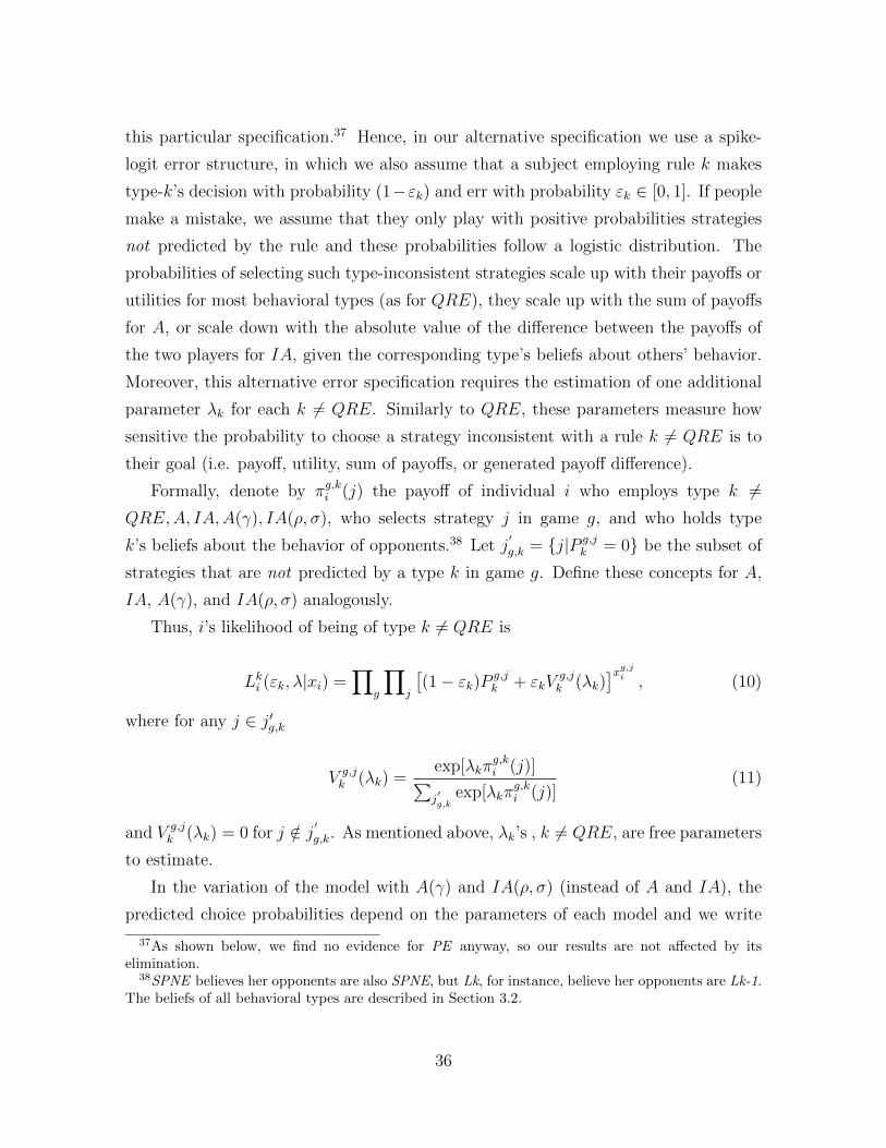
this particular specification.37 Hence, in our alternative specification we use a spike-

logit error structure, in which we also assume that a subject employing rule k makes

type-k’s decision with probability (1−εk) and err with probability εk ∈ [0, 1]. If people

make a mistake, we assume that they only play with positive probabilities strategies

not predicted by the rule and these probabilities follow a logistic distribution. The

probabilities of selecting such type-inconsistent strategies scale up with their payoffs or

utilities for most behavioral types (as for QRE), they scale up with the sum of payoffs

for A, or scale down with the absolute value of the difference between the payoffs of

the two players for IA, given the corresponding type’s beliefs about others’ behavior.

Moreover, this alternative error specification requires the estimation of one additional

parameter λk for each k 6= QRE. Similarly to QRE, these parameters measure how

sensitive the probability to choose a strategy inconsistent with a rule k 6= QRE is to

their goal (i.e. payoff, utility, sum of payoffs, or generated payoff difference).

Formally, denote by πg,ki (j) the payoff of individual i who employs type k 6=QRE,A, IA,A(γ), IA(ρ, σ), who selects strategy j in game g, and who holds type

k’s beliefs about the behavior of opponents.38 Let j′

g,k = {j|P g,jk = 0} be the subset of

strategies that are not predicted by a type k in game g. Define these concepts for A,

IA, A(γ), and IA(ρ, σ) analogously.

Thus, i’s likelihood of being of type k 6= QRE is

Lki (εk, λ|xi) =∏

g

∏j

[(1− εk)P g,j

k + εkVg,jk (λk)

]xg,ji , (10)

where for any j ∈ j′g,k

V g,jk (λk) =

exp[λkπg,ki (j)]∑

j′g,k

exp[λkπg,ki (j)]

(11)

and V g,jk (λk) = 0 for j /∈ j ′g,k. As mentioned above, λk’s , k 6= QRE, are free parameters

to estimate.

In the variation of the model with A(γ) and IA(ρ, σ) (instead of A and IA), the

predicted choice probabilities depend on the parameters of each model and we write

37As shown below, we find no evidence for PE anyway, so our results are not affected by itselimination.

38SPNE believes her opponents are also SPNE, but Lk, for instance, believe her opponents are Lk-1.The beliefs of all behavioral types are described in Section 3.2.

36

P gk (θ) being θ = γ and θ = (ρ, σ), respectively. The expression (10) then becomes:

Lki (εk, θ, λk|xi) =∏

g

∏j

[(1− εk)P g,j

k (θ) + εkVg,jk (λk)

]xg,ji , (12)

The QRE probabilities are defined as in (6) and (7) and, by analogy, the log-

likelihood of the whole sample under A and IA is

lnL(p, (εk)k 6=QRE, λ|x) =∑

iln[∑

k 6=QREpkL

ki (εk, λk|x

g,ji ) + pQREL

QREi (λQRE|xg,ji )

].

(13)

In case of A(γ) and IA(ρ, σ), the log-likelihood (13) changes to

lnL(p, (εk)k 6=QRE, γ, ρ, σ, λ|x) =∑

iln[∑

pkLki (.)]

. (14)

5.3.2 Estimation Results

We estimate two sets of parameters: frequency of behavioral types within the subject

population p = (p1, p2, ..., pK) and the error-related parameters, one or two for each

behavioral type depending on the error specification. Under uniform errors, the error-

related parameters are εk for k 6= QRE and the inverse error rate λ for QRE. In

contrast, under the spike-logit specification, there are two error-related parameters per

model, with the exception of QRE. More precisely, εk for k 6= QRE and a vector

λ = (λ1, ..., λK) that includes λQRE. Last, if A(γ) and IA(ρ, σ) are applied, we also

estimate their parameters. Under mild conditions satisfied by the functions (8), (9),

(13), and (14), the maximum likelihood estimation produces consistent estimates of

the parameters (Leroux, 1992).

Tables 6A and 6B present the estimation results for both error specifications. Table

6A corresponds to estimations with A and IA; Table 6B to those with the parameter-

ized A(γ) and IA(ρ, σ). Columns (1− 4) in Table 6A and columns (1− 6) in Table 6B

contain the uniform-error specification estimates, while columns (5− 10) and (7− 14),

respectively, show those for spike-logit errors. Standard errors shown in parentheses

below each estimate and the corresponding significance levels (**p > 0.01, *p > 0.05)

were computed using bootstrapping with 100 replications (Efron and Tibshirani, 1994).

For the frequency parameters pk, the inverse error rates λQRE, and for parameters γ,

37

ρ, and σ, we simply report their significance levels. However, the error rates are well

behaved if they are close to zero and far from one. Therefore, we test whether each εk

differs significantly from one (rather than zero). The standard errors and significance

levels reported jointly with the estimated εk’s in Tables 6A and 6B correspond to these

tests.39

There are several differences between the uniform and spike-logit error specifica-

tions. They mainly differ in how they treat choices inconsistent with a type k. The

former treats all mistakes in the same way, while the latter punishes more costly mis-

takes more than less costly ones. The consequence of the payoff-dependent errors is

that the spike-logit specification uses more information, since it regards the payoffs.40

Rather than favoring one error specification over the other, we let readers decide, in

which assumptions they wish to place more confidence.

We first discuss in detail the results from Table 6A. First, consider the models that

include all the behavioral types introduced in Section 3.2, shown in columns (1 − 2)

and (5 − 7) in Table 6A. Observe that both error specifications yield qualitatively

similar results. First, non-strategic and preference-based behavioral models (A, IA,

PE, O) all explain less than 5%. IA and PE additionally exhibit very high error rates.

The O type is an exception in that, despite explaining only 3% of the population, its

estimated fractions are significant and the error rates very low. Moreover, its estimates

are highly robust to the model specification. Second, SPNE explains the behavior of

about 10% of subjects well, consistently across the two models, and SPNE ’s estimated

error rates are actually among the lowest. Third, the rest of the behavior–in fact,

most of the behavior of subjects inconsistent with SPNE–is best explained by level-k

thinking and QRE. Under both error specifications, level-k thinking is estimated to

represent around 55% of the subject population, while QRE represents about 30%.

Level-k thinking model also shows a familiar pattern compared to other estimation

results with most subjects concentrated in L1, followed by L2 and L3 (see Crawford et

39We perform no statistical tests for the λk’s corresponding to the models different from QRE inthe spike-logit specification because these only tell how sensitive the mistakes are to each type’s goal,but they are irrelevant for telling with which probability people make mistakes. These probabilitiesare determined by the estimated εk.

40Another potential difference might arise due to the joint estimation of λ with the other parametersif the estimated λ differs across the two models. The value of λ affects the degree of separabilitybetween QRE and the other candidates (see Table A1) and different separability may effect theestimated type frequencies. Since the estimated λ’s are very similar in all our estimations, thisconcern does not apply here.

38

Table 6A: Estimation Results I: Non-Parameterized Specification for Social Preferences

Uniform Error Spike-Logit ErrorFull Selected Full Selected

Type pk εk, λ pk εk, λ pk εk λk pk εk λk(1) (2) (3) (4) (5) (6) (7) (8) (9) (10)

SPNE 0.09** 0.32** 0.08** 0.31** 0.10** 0.27** 1.00 0.11** 0.29** 0.98(0.03) (0.09) (0.03) (0.08) (0.03) (0.05) (0.02) (0.04) (0.06) (0.08)

A 0.02 0.38** 0.01 0.19** 0.02(0.01) (0.19) (0.01) (0.04) (0.20)

IA 0.03** 1.00 0.02 0.80** 0.00(0.01) (0.20) (0.01) (0.06) (0.05)

PE 0.00 0.75*(0.02) (0.15)

O 0.03* 0.06** 0.03* 0.06** 0.03* 0.05** 0.08 0.03* 0.05** 0.08(0.01) (0.11) (0.01) (0.17) (0.01) (0.08) (0.14) (0.01) (0.07) (0.14)

L1 0.29** 0.59** 0.31** 0.60** 0.41** 0.49** 0.01 0.43** 0.51** 0.01(0.05) (0.04) (0.05) (0.05) (0.07) (0.03) (0.05) (0.07) (0.03) (0.06)

L2 0.18** 0.61** 0.21** 0.66** 0.08** 0.36** 0.19 0.08** 0.36** 0.19(0.06) (0.06) (0.06) (0.04) (0.02) (0.04) (0.08) (0.03) (0.04) (0.08)

L3 0.10* 0.59** 0.11* 0.62** 0.06* 0.43** 0.01 0.06* 0.44** 0.00(0.04) (0.08) (0.04) (0.07) (0.04) (0.12) (0.02) (0.04) (0.12) (0.01)

QRE 0.28** 0.38** 0.27** 0.42** 0.29** 0.39** 0.29** 0.37**(0.05) (0.12) (0.05) (0.15) (0.05) (0.09) (0.06) (0.09)

al., 2013). However, the main difference between both error specifications comes from

the proportions of each level. Under uniform errors, around half of the population best

explained by level-k is classified as L1, while L1 absorbs half of the shares of L2 and

L3 in the spike-logit specification.

Given that several models systematically fail to explain the behavior in our exper-

iment, we estimate reduced models with some selected behavioral types. One widely

debated and so far unresolved issue is the over-parameterization of mixture-of-types

models and the related model selection (MacLachlan and Peel, 2000; Cameron and

Trivendi, 2005, 2010).41 Cameron and Trivendi (2005) propose using the natural in-

terpretation of the parameters and MacLachlan and Peel (2000) argue that the best

model minimizes the number of components selected if their proportions differ and all

are different from zero. We take an approach that combines these recommendations.

We require two conditions to hold for a type k to be included in our reduced model:

pk >> 0 and εk << 1 (λk >> 0 for QRE). In words, we require the share of each type

41Standard criteria for model selection (such as Aikake or Bayesian Information criteria or thelikelihood ratio test) may perform unsatisfactorily in finite mixture models (Cameron and Trivendi,2005, 2010).

39

k selected to be high enough and its error rate low enough (the inverse error rate high

enough for QRE) to suggest that the decisions of people classified as k are made on

purpose rather than by error.42

For both specifications, we eliminate those rules with negligible shares or high error

rates. In particular, we estimate a reduced form of both (8) and (13), in which we only

include the relevant behavioral types O, QRE, level-k, and SPNE. Columns (3−4) and

(8− 10) in Table 6A report the results. The estimates of the selected behavioral types

are stable as we move from the full to the reduced model. Moreover, all the parameters

estimated are well behaved. Under the uniform specification, the types excluded are

entirely absorbed by L1 and L2. As a result, their error rates slightly increase. The

estimates suggest that the composition of the population is 3% of O, 8% of SPNE, 27%

of QRE, and 63% of level-k. Under the spike-logit specification, the types excluded are

entirely absorbed by L1 and SPNE and their error rates thus slightly increase. The

estimates suggest that the composition of the population is 3% of O, 11% of SPNE,

29% of QRE, and 57% of level-k reasoning, figures very similar to the uniform-error

specification.43

Let us now turn the attention to Table 6B, in which we consider the flexible models

of social preferences A(γ) and IA(ρ, σ). In Table 6B, the uniform-error specification

is positioned in the top of the table while the spike-logit specification in the bottom.

Observe that the estimates of each estimation are displayed in three columns; columns

(1− 3) and (7− 10) correspond to the full models and columns (4− 6) and (11− 14)

to the selected ones. In line with Table 6A, the estimates are robust to the error

specification and the elimination of rules from the full model. Most importantly, the

majority of non-equilibrium behavior is still explained by level-k and QRE and their

estimated parameters are virtually unaffected.

42This approach follows Kovarik et al. (2018) who propose a related model-selection algorithm and,using Monte-Carlo simulations, show that such an algorithm successfully recovers the data-generatingprocesses as long as the error rates are not too high.

43It might be thought that our comparison between QRE and level-k could favor the latter, as level-k allows for multiple types while we estimate a single QRE. Therefore, we re-estimate our uniformmodel with two QRE types (with different λ’s). The estimation results are shown in Table A6 in theAppendix A. Compared to the original pQRE = 0.27 and λQRE = 0.42, the introduction of anotherQRE type leads to pQRE1 = 0.22 with λQRE1 = 0.38 and pQRE2 = 0.06 with λQRE2 = 0.32, while theestimated frequencies of the rest of the types being virtually unaffected. Therefore, the proportion ofpeople classified in each rule is unaffected by considering one or two QRE types and our benchmarkmodel does not seem to favor level-k over QRE.

40

Table 6B: Estimation Results II: Parameterized Specification for Social Preferences

Uniform ErrorFull Selected

Type pk εk, λ γ, ρ, σ pk εk, λ γ, ρ, σ(1) (2) (3) (4) (5) (6)

SPNE 0.01 0.00**(0.01) (0.15)

A 0.08** 0.38** 0.21** 0.08** 0.38** 0.22**(0.03) (0.07) (0.04) (0.03) (0.07) (0.04)

IA 0.06** 0.20** 0.07**,0.55** 0.06** 0.18** 0.08**,0.55**(0.02) (0.03) (0.02),(0.12) (0.03) (0.04) (0.02),(0.13)

PE 0.01 0.45**(0.02) (0.23)

O 0.03* 0.06** 0.03* 0.06**(0.01) (0.07) (0.01) (0.10)

L1 0.28** 0.59** 0.29** 0.59**(0.04) (0.04) (0.05) (0.04)

L2 0.20** 0.65** 0.21** 0.67**(0.06) (0.08) (0.05) (0.07)

L3 0.08* 0.63** 0.08* 0.62**(0.04) (0.13) (0.04) (0.14)

QRE 0.24** 0.37** 0.24** 0.38**(0.04) (0.09) (0.05) (0.09)

Spike-Logit ErrorFull Selected

Type pk εk λk γ, ρ, σ pk εk λk γ, ρ, σ(7) (8) (9) (10) (11) (12) (13) (14)

SPNE 0.06** 0.93** 0.49 0.06** 0.93** 0.34(0.01) (0.03) (0.03) (0.01) (0.04) (0.03)

A 0.10** 0.39** 0.01 0.29** 0.10** 0.11** 0.00 0.19**(0.01) (0.01) (0.01) (0.00) (0.02) (0.05) (0.10) (0.01)

IA 0.06** 0.12** 0.51 0.02,0.76** 0.06** 0.11** 0.53 0.02,0.80**(0.01) (0.01) (0.02) (0.00),(0.00) (0.00) (0.01) (0.04) (0.01),(0.00)

O 0.03** 0.05** 0.08 0.03** 0.05** 0.08(0.01) (0.04) (0.02) (0.01) (0.02) 0.04

L1 0.37** 0.47** 0.01 0.37** 0.47** 0.01(0.01) (0.02) (0.01) (0.08) (0.02) (0.05)

L2 0.09** 0.37** 0.14 0.09** 0.37** 0.14(0.01) (0.02) (0.03) (0.00) (0.03) (0.03)

L3 0.00 0.63** 0.10**(0.00) (0.03) (0.03)

QRE 0.29** 0.34** 0.29** 0.34**(0.02) (0.06) (0.06) (0.03)

41

The main difference between Tables 6A and 6B concerns SPNE and the social-

preference types. We find no evidence for A and IA in Table 6A, whereas 14% of

subjects are classified as either A(γ) or IA(ρ, σ) and their error rates are well behaved

in Table 6B. We can observe that these shares come at the cost of SPNE, which

receives no support in the full model and is, therefore, eliminated in the selected one.

However, a closer look at the estimated γ, ρ, and σ of subjects classified into these

social-preference types reveals the reason: they exhibit almost no social concerns and

their behavior matches closely that of SPNE. As shown in Tables 2, 3, and 4, SPNE

and IA(ρ = 0.08, σ = 0.55) predict exactly the same strategy in 30 decisions (out of 32)

whereas SPNE and A(γ = 0.22) in 26 of them. Moreover, in the remaining cases (with

one exception) both A(γ = 0.22) and IA(ρ = 0.08, σ = 0.55) predict multiple actions,

one of which is typically the same as the one prescribed by SPNE. That is, even if

A(γ) and IA(ρ, σ) could theoretically be well separated from SPNE (simply by being

truly non-selfish; see Tables A2 and A3 in the Appendix A), the actually estimated

altruistic and inequity-averse types become behaviorally almost indistinguishable in

order to explain about 14% of the population. They thus account for a very small part

of non-equilibrium choices in our data. Most importantly though, since these social-

preference types only compete for space with SPNE and never with the other non-

SPNE theories, the conclusions that most non-equilibrium choices can be explained

by the failure of common knowledge of rationality (level-k) and bounded rationality

(QRE) and preference-based arguments play at most a negligible role in explaining non-

equilibrium play in CGs still hold even if we allow for more flexible social-preference

types.

An issue linked naturally to the objectives of finite-mixture modeling is whether the

estimations generate a well separated, non-overlapping classification of subjects at the

individual level. In particular, a desirable property of type mixtures is that individuals

are ex-post classified to one and only one of the candidate types, rather than, say,

50% QRE and 50% level-k. Therefore, we compute posterior probabilities of each

individual belonging to a certain type (see MacLachlan and Peel, 2000). Given that our

two specifications in Tables 6A and Tables 6B deliver qualitatively and quantitatively

similar results, this exercise is only performed for the selected model under uniform

errors in Table 6A. If people are accurately classified at the individual level then those

posterior probabilities are close to one for a single behavioral model and close to zero

42

for the remaining ones for each individual. This is indeed the case here (see Figure

A8) so we conclude that our classification is also successful at the individual level. As

a result, two departures from SPNE seem to be crucial for non-equilibrium behavior

in CGs and, as shown by this posterior-probabilities exercise, each model is relevant

for different individuals.

5.3.3 Robustness 1: Estimation by Player Role and Omitted Types

In this section, we provide two additional exercises. First, we estimate the selected

models separately for the two player roles. Second, we report an exercise testing for

omitted behavioral types. Since all our model specifications deliver similar messages,

the robustness checks in this section are only performed for the selected models from

Table 6A.

Estimation by player role. There is some evidence that people adapt their so-

phistication to their strategic situations (see e.g. Kovarik et al., 2018, or Mengel and

Grimm, 2012).44 Since this might potentially also apply to different roles in the same

game, we would like to make sure that our conclusions still hold if we re-estimate our

selected models separately for each player role. Table 7 reports the estimates for both

the uniform and spike-logit error specifications. Observe that our main conclusions are

qualitatively unaffected by only considering one player type: a relatively small fraction

of subjects is classified as SPNE, while the majority is best described by either QRE

or level-k. Again, level-k is the most relevant model, classifying most people as L1.

However, we observe two systematic quantitative differences across the player roles. In

particular, Players 2 exhibit higher estimated shares of L1 and lower shares of L3. In

fact, the estimates suggest that no subject in role 2 can be classified as L3.45

To see whether the type composition changes across the two player roles, we for-

mally test whether the parameters estimated differ across the two models, using the

uniform error specification. Brame et al. (1998) propose a statistical test for the equal-

ity of maximum-likelihood regression coefficients between two independent equations.

Despite the differences mentioned above, these tests detect no difference between the

corresponding pairs of estimated coefficients across the two models at the conventional

44Gill and Prowse (2016) document that some people change their degree of sophistication dependingon the sophistication of their opponents in Beauty Context Games.

45The available data do not allow us to explore the reason behind the differences.

43

5% level, with the exception of the error rate of L1, εL1. These tests thus support the

idea that the above classification differ neither qualitatively nor quantitatively across

the two player roles.

Table 7: Estimation Results by Subjects’ Role: Player 1 and Player 2

Uniform Error Spike-Logit ErrorPlayer 1 Player 2 Player 1 Player 2

Type pk εk, λ pk εk, λ pk εk λ pk εk λSPNE 0.05* 0.33** 0.05 0.16** 0.05 0.23** 1.00 0.14** 0.26** 0.93

(0.03) (0.09) (0.06) (0.15)) (0.03) (0.17) (0.03) (0.05) (0.09) (0.10)O 0.05* 0.33** 0.05 0.16** 0.03* 0.00** 0.26 0.03 0.09** 0.08

(0.03) (0.09) (0.06) (0.15)) (0.01) (0.20) (0.17) (0.02) (0.12) (0.11)L1 0.31** 0.81** 0.44** 0.54** 0.31** 0.61** 0.01 0.44** 0.44** 0.05

(0.07) (0.04) (0.09) (0.05)) (0.08) (0.04) (0.04) (0.06) (0.02) (0.06)L2 0.10* 0.60** 0.23** 0.66** 0.10* 0.41** 0.16 0.06* 0.26** 0.42

(0.06) (0.14) (0.08) (0.09)) (0.05) (0.05) (0.09) (0.02) (0.11) (0.15)L3 0.22** 0.58** 0.05 0.69* 0.21* 0.45** 0.01 0.00 0.51** 0.05

(0.09) (0.03) (0.03) (0.15)) (0.10) (0.08) (0.02) (0.00) (0.15) (0.07)QRE 0.33** 0.38** 0.23** 0.67** 0.31** 0.38** 0.33** 0.27

(0.07) (0.10) (0.05) (0.15)) (0.06) (0.10) (0.06) (0.17)

Omitted types. One important question inherent in finite mixture-of-types mod-

els is the selection of the candidate types. What if there is a type that explains a

relevant part of our subjects’ behavior but is not included in the set of candidate

explanations?

To test for this possibility, we perform the following “omitted type” exercise. We

re-estimate our models separately for each player role 76 and 75 times for Player 1 and

Player 2, respectively. In each of these 151 estimations, we add to the set of considered

models an additional type, whose predicted behavior is identical to the experimental

behavior of one particular subject’s choices. That is, each subject represents one type

in one these 151 estimations. If someone’s behavior approximates the behavior of many

others well and is sufficiently different from any of the theories considered, this would

provide evidence for a relevant type being missing from our set. Note that this exercise

is only possible under the uniform error specification because we take the behavioral

profile as a type without actually observing the underlying optimization problem of

such subjects.

For such an omitted type to be relevant, two criteria are applied. First, we require

the type to attract a non-negligible frequency. In particular, we look for subjects

who attract a share of at least 10% the population. Second, we require the type to be

44

sufficiently separated from any candidate explanation already considered. In particular,

types must be separated in at least half of the 16 CGs. It turns out that there are five

subjects who play as Player 1 (subjects 10, 17, 39, 67 and 72) and three who play as

Player 2 (subjects 100, 140, 151), who satisfy both conditions. A closer look at their

behavior reveals that they all behave as hybrids between different consecutive types

of level-k. When we add those two combinations as possible behavioral types, L1 -L2

and L2 -L3, which consist of either one type or the other, none of the predictions of

the omitted types survives the application of the separation criteria mentioned above.

Hence there are some subjects whose behavior taken as a behavioral type could po-

tentially explain that of a non-negligible part of other subjects. However, these omitted

types hybridize level-k and mostly affect the share of different level-k types, such that

they still maintain the assumption of perfect rationality and relax the common knowl-

edge of rationality.46 Therefore, their existence does not affect our main conclusions

in that equilibrium behavior is represented by a minority and that the majority of

individuals can be explained by either level-k or QRE.

5.3.4 Robustness 2: Out-of-Sample Predictions

The ability to predict out-of-sample is a desirable feature of any model. In this section,

we assess the extent to which the selected uniform-error mixture model (columns (3 -

4) in Table 6A) that best fits the behavior of subjects in some games, referred to as

in-sample games, is able to predict both individual and population-level behavior in

other games, referred to as out-of-sample games. For this model to generate successful

out-of-sample predictions, we require two things. First, the estimated composition

of the population, as well as the individual posterior probabilities of belonging to

a particular behavioral type must be stable across different in-sample games. This

would actually show how robust the estimates of our mixture-of-types model in Table

6A is to the removal of one particular game. Second, this model must predict behavior

successfully in and consistently across different out-of-sample games, at both individual

and population level.47

46See Gill and Prowse (2016) for further evidence on these hybrid types. A finer analysis of thesehybrid types is out of the scope of the present paper.

47There only exists scarce evidence of whether subjects’ behavior is stable across different games.Georganas et al. (2015) examine whether level-k model generates stable cross-game predictions at theindividual level in two types of games (undercutting games and two-person guessing games). They

45

The individual- and population-level out-of-sample prediction exercises that we

carry out exploit the behavioral variation across the 16 different CGs used in our

experiment and have the following common basis. First, we estimate 16 variations of

the model with 15 games only (rather than 16 as in Table 6A). Since we remove a

different game each time from each estimation, this yields 16 different population-level

estimations, reported in Tables A7 and A8 in the Appendix A.

We first check the robustness of the estimates to such removals. At the population

level, we formally test whether any of the parameters estimated in these 16 models

is significantly different from its counterpart in the benchmark model in columns (3

- 4) in Table 6A. It is remarkable that none of the 16 × 12 = 192 parameters is

significantly different at conventional 5% from its original estimation with 16 games.48

At the individual level, we employ the parameters estimated in the 16 models based on

15 games and compute the posterior probabilities of our 151 subjects belonging to each

behavioral type.49 For each of the 16 models, we assign each individual to the type

that best explains his/her behavior in the in-sample games. This enables us to assess

the individual-level stability and consistency of our classification from the previous

section. We observe that 42% of the subjects (63 out of 151) are fully consistent, such

that they are classified in the same behavioral type across all 16 estimations; 77%

(117 out of 151) are consistently classified in at least 12 out of 16 (75%) games. Most

of our subjects are thus consistently classified into the same behavioral model at the

individual level even in subsets of our games. Therefore, our main estimation results

are highly robust to the removal of any single game at both the population and the

individual level.

Individual-level out-of-sample predictions. We use the above individual-level

classification of subjects based on the 15 in-sample games and predict the strategy

that each subject should take in the out-of-sample CG excluded while making the

classification. Our individual-level test compares this predicted behavior with the

action actually taken by the corresponding subject in the corresponding game. This

exercise generates a 151 × 16 matrix of “hits”, or “probability of hits” for QRE, for

report stable classification within types but large instability across game types. Given these results,our out-of-sample exercise solely focuses on different CGs.

48We do not report the details of these 192 tests here. They are available upon request from theauthors.

49This would lead to 16 four-panel graphs similar to Figure A8 in the Appendix A.

46

the 151 subjects in the 16 CGs, which enables us to assess the ability of the mixture-

of-types model to predict the behavior of each subject in the out-of-sample CGs.

To provide a relative prediction performance of our mixture model, we repeat this

procedure for each relevant behavioral type (SPNE, QRE, O, and level-k) in isolation.

For SPNE and O, we simply take the average compliance between their predictions

and actual individual behavior across the 16 CGs. For QRE we estimate 16 models

that assume that all subjects are classified as QRE using their observed behavior in the

in-sample games, yielding one λ per estimation. With the estimated λ’s, we assess the

average ability of QRE to predict the observed behavior in the out-of-sample CGs. For

level-k, we estimate 16 mixture models with three types, L1, L2, and L3, and compute

accordingly the average individual-level ability of this level-k mixture to predict out of

sample.

The left panel of Figure 6 reports the average improvement in the ability to predict

individual behavior out of sample (in percentage terms) in each model, be it our mixture

model or one of the four one-type models described above, compared to a pure random

hit of 0.25. The latter corresponds to a purely random type that selects each strategy

with probability one fourth. The figures reported should thus be interpreted as how

much better in percentage points the out-of-sample prediction of a particular model

is than a pure random selection of action. The vertical bars reflect standard errors

of the 16 improvements and reflect how sensitive the ability of each model to predict

individual out-of-sample behavior is to different out-of-sample CGs. A good model

should on average exhibit significantly greater improvements with respect to random

behavior and the average improvement should not be too sensitive to which game

is being predicted. Our mixture and the mixture of different level-k’s exhibit the

largest improvements compared to random prediction, but a comparison between them

shows that allowing non-level-k types in our mixture model improves the ability to

predict individual behavior significantly. Our mixture model improves the prediction

ability of a radnom type by almost 90%, compared to less than 80% in case of level-

k. Additionally, our mixture-of-types model and QRE reveal the lowest sensitivity to

which CG is being predicted. However, our mixture-of-types model largely outperforms

QRE. We thus conclude that jointly considering alternative explanations of behavior

significantly enhances the ability of a model to predict individual behavior in out-of-

sample games.

47

Population-level out-of-sample predictions. This test is again based on the

16 estimations with the 15 in-sample games described above.50 With the estimates in

hand, we compute the log-likelihood (8) for the observed behavior of our subjects in

the out-of-sample game. This generates 16 log-likelihood values. Again, to be able to

assess the relative ability of the mixture-of-types model in columns (3 - 4) in Table

6A to predict out of sample vis-a-vis the individual explanations of behavior in the

in-sample games, we apply the estimated parameters and compute the loglikelihood

of the observed behavior in the out-of-sample CG. As before, we preform the same

exercise for a random type, which selects each strategy with probability one fourth,

and use it for normalization. More precisely, we compute the difference between the

log-likelihood of each model (once again either our mixture model or all the one-type

models) and the log-likelihood of the uniform model divided by the log-likelihood of

the uniform model, which gives the percentage improvement in log-likelihoods of each

model with respect to random behavior. The right-hand panel of Figure 6 reports the

average percentage improvement of the log-likelihood values with respect to random

behavior (see Table A9 for more details). The vertical bars reflect the standard errors

of these 16 improvements and again reflect how sensitive the ability of each model to

predict is to the CG considered. A good model should on average exhibit significantly

greater improvement with respect to random behavior and the average improvement

should not be too sensitive to which game is being predicted. In the latter case, if the

standard errors are large the particular model predicts well for some games but fails to

predict successfully for others. Observe that the first condition is only satisfied for the

mixture-of-types model and a mixture of level-k. That is, QRE, SPNE, and O alone

are not significantly better at predicting the behavior of our subjects out-of-sample

than a random selection of an action. Furthermore, the mixture-of-types model on

average outperforms the level-k alone.

As for standard errors, the mixture-of-types model is also the most stable at pre-

dicting behavior, while all the others show greater sensitivity to the out-of-sample

games. In fact, our mixture-of-types model is the only one that always outperforms

the random type (see Table A9). The remaining models always predict the behavior

50This exercise is motivated by Wright and Leyton-Brown (2010) except that we predict the behaviorof the same subjects in different games, rather than using one part of the subject pool for predictingthe behavior of other part of the pool.

48

Mix

ture

-of-t

ypes

QRE

SPNE O

Level-k

−0.2

0

0.2

0.4

0.6

0.8

1

Individual-level

Mix

ture

-of-t

ypes

QRE

SPNE O

Level-k

−0.1

0

0.1

Population-level

Figure 6: Average Percentage Improvement in the Ability to Predict (left) and Log-likelihood (right) over the Random Behavior, when Comparing the Observed Behaviorin out-of-sample Games Using in-sample Games for Estimation.

worse than a pure random type for at least two games.51 This includes the mixture of

level-k.

We thus conclude that, at both the individual and population levels, our mixture-

of-types model is the most successful in predicting behavior and the least dependent on

which out-of-sample game is chosen to predict. As a result, researchers should account

for behavioral heterogeneity in CGs not only for a better explanation of behavior as

advocated by this paper, but also for a better prediction of choices in out-of-sample

games.

6 Conclusions

We report a study designed to explain initial behavior in CGs, combining experimental

and econometric techniques. Our approach enables us to classify people into different

behavioral explanations and discriminate between them. Crucially, this approach deter-

mines endogenously whether one or multiple explanations are empirically relevant. We

show that people are largely heterogeneous and more than one explanation is required

to both explain and predict individual behavior in CGs. Independently of our model

51O is an exception but it is because the estimated error is εo = 1. Therefore, it always performsas the random behavioral type.

49

specification, roughly 10% of people behave close to SPNE and most non-equilibrium

behavior seems to be due to two reasons: either the failure of common knowledge of

rationality, as advocated by Aumann (1992, 1995) and modeled via level-k thinking

model in our setting, or bounded reasoning abilities of subjects, simulated by QRE.

The reported results may stimulate future research in two directions. Our study

contributes to the “competition” between level-k models and QRE as two behavioral

alternatives to standard equilibrium approaches. Some authors argue for the former

while others prefer the latter, but empirical literature has found difficulties in discrim-

inating between the two approaches because both theories often predict very similar

behavior. As a result, most studies compare their abilities to explain behavior using

the representative-agent approach. Our design allows us to separate the predictions

of the two theories and we show that–at least in our setting–both level-k models and

QRE are empirically relevant for the explanation of non-equilibrium choices but each

model explains the behavior of different subjects. Future research should determine

how these conclusions extend to other strategic contexts.

Second, the behavior in CGs and other extensive-form games have been attributed

to their dynamic nature and the failure of backward induction, whereas our study

again shows that it may be a more general non-equilibrium phenomenon. Since most

non-equilibrium choices in our experiment are best explained by QRE and level-k that

have been successful in explaining behavior in static environments, our findings call

for a reevaluation of the aspects that distinguish static from dynamic games in the

analysis of non-equilibrium behavior.

References

[1] Aumann, R. (1988). Preliminary notes on integrating irrationality into game the-

ory. In International Conference on Economic Theories of Politics, Haifa.

[2] Aumann, R. J. (1992). Irrationality in Game Theory. In Economic Analysis of

Markets and Games: Essays in Honor of Frank Hahn, ed. Partha Dasgupta, Dou-

glas Gale, Oliver Hart and Eric Maskin, 214-27. Cambridge: MIT Press.

[3] Aumann, R. J. (1995). Backward Induction and Common Knowledge of Rational-

ity. Games and Economic Behavior 8: 6-19.

50

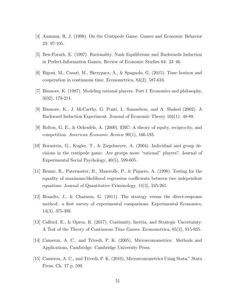
[4] Aumann, R. J. (1998). On the Centipede Game. Games and Economic Behavior

23: 97-105.

[5] Ben-Porath, E. (1997). Rationality, Nash Equilibrium and Backwards Induction

in Perfect-Information Games. Review of Economic Studies 64: 23–46.

[6] Bigoni, M., Casari, M., Skrzypacz, A., & Spagnolo, G. (2015). Time horizon and

cooperation in continuous time. Econometrica, 83(2), 587-616.

[7] Binmore, K. (1987). Modeling rational players: Part I. Economics and philosophy,

3(02), 179-214.

[8] Binmore, K., J. McCarthy, G. Ponti, L. Samuelson, and A. Shaked (2002). A

Backward Induction Experiment. Journal of Economic Theory 104(1): 48-88.

[9] Bolton, G. E., & Ockenfels, A. (2000). ERC: A theory of equity, reciprocity, and

competition. American Economic Review 90(1), 166-193.

[10] Bornstein, G., Kugler, T., & Ziegelmeyer, A. (2004). Individual and group de-

cisions in the centipede game: Are groups more “rational” players?. Journal of

Experimental Social Psychology, 40(5), 599-605.

[11] Brame, R., Paternoster, R., Mazerolle, P., & Piquero, A. (1998). Testing for the

equality of maximum-likelihood regression coefficients between two independent

equations. Journal of Quantitative Criminology, 14(3), 245-261.

[12] Brandts, J., & Charness, G. (2011). The strategy versus the direct-response

method: a first survey of experimental comparisons. Experimental Economics,

14(3), 375-398.

[13] Calford, E., & Oprea, R. (2017). Continuity, Inertia, and Strategic Uncertainty:

A Test of the Theory of Continuous Time Games. Econometrica, 85(3), 915-935.

[14] Cameron, A. C., and Trivedi, P. K. (2005), Microeconometrics: Methods and

Applications, Cambridge: Cambridge University Press.

[15] Cameron, A. C., and Trivedi, P. K, (2010), Microeconometrics Using Stata,” Stata

Press, Ch. 17 p. 599.

51

[16] Cooper, R., DeJong, D. V., Fosythe, R. & Ross, T. W. (1996), Cooperation with-

out reputation: experimental evidence from prisoners dilemma games, Games

and Economic Behavior 12(2), 187218.

[17] Costa-Gomes, M. A., V. P. Crawford, and B. Broseta (2001), “Cognition and

behavior in normal-form games: An experimental study,” Econometrica, 69: 1193–

1235.

[18] Crawford, V.P., M. A. Costa-Gomes and N. Iriberri (2013), “Structural Models of

Non-equilibrium Strategic Thinking:Theory, Evidence, and Applications,” Journal

of Economic Literature, 51:1: 5–62.

[19] Dal Bo, P., & Frechette, G. R. (2011). The evolution of cooperation in infinitely

repeated games: Experimental evidence. The American Economic Review, 101(1),

411-429.

[20] Danz, D., Huck, S., & Jehiel, P. (2016). Public Statistics and Private Experi-

ence: Varying Feedback Information in a Take-or-Pass Game. German Economic

Review, 17(3), 359-377.

[21] Efron, B. and Tibshirani, R. J., (1994), An Introduction to the Bootstrap, Chap-

man & Hall/CRC.

[22] El-Gamal M.A. and D.M. Grether (1995) Are People Bayesian? Uncovering Be-

havioral Strategies. Journal of the American Statistical Association 90: 1137–1145.

[23] Embrey, M., Frechette, G. R., & Yuksel, S. (2017). Cooperation in the finitely

repeated prisoner’s dilemma. Quarterly Journal of Economics, forthcoming.

[24] Fey, M., R.D. McKelvey and T. Palfrey, (1996), “An Experimental Study of

Constant-sum Centipede Games,” International Journal of Game Theory, 25:

269–287.

[25] Fischbacher, U., (2007), “z-Tree: Zurich toolbox for ready-made economic exper-

iments,” Experimental Economics, 10(2): 171–178.

[26] Friedman, D., & Oprea, R. (2012). A continuous dilemma. The American Eco-

nomic Review, 102(1), 337-363.

52

[27] Gill, D., & Prowse, V. L. (2016). Cognitive ability, character skills, and learning to

play equilibrium: A level-k analysis. Journal of Political Economy, forthcoming.

[28] Goeree, J.K. and Holt, C.A., (2001), Ten little treasures of game theory and ten

intuitive contradictions. American Economic Review 91: 1402-1422.

[29] Greiner, B., (2015), “Subject Pool Recruitment Procedures: Organizing Experi-

ments with ORSEE,” Journal of the Economic Science Association, 1(1): 114–125.

[30] Grimm, V., and Mengel, F. (2012). An experiment on learning in a multiple games

environment. Journal of Economic Theory, 147(6), 2220-2259.

[31] Harless, D. W., & Camerer, C. F. (1994). The predictive utility of generalized

expected utility theories. Econometrica 62, 1251-1289.

[32] Healy, P.J. (2017). Epistemic Experiments: Utilities, Beliefs, and Irrational Play,

mimeo, Ohio State University.

[33] Georganas, S., P. J. Healy, and R. Weber. (2015). On the Persistence of Strategic

Sophistication. Journal of Economic Theory 159, 369-400.

[34] Ho, T. H., and Su, X. (2013). A dynamic level-k model in sequential games.

Management Science, 59(2), 452-469.

[35] Iriberri, N., and Rey-Biel, P. (2013). Elicited beliefs and social information in

modified dictator games: what do dictators believe other dictators do. Quantitative

Economics 4: 515-547.

[36] Jehiel, P. (2005). Analogy-based expectation equilibrium. Journal of Economic

theory, 123(2), 81-104.

[37] Johnson, E. J., C. Camerer, S. Sen, and T. Rymon (2002). Detecting Failures

of Backward Induction: Monitoring Information Search in Sequential Bargaining.

Journal of Economic Theory 104: 16-47.

[38] Kawagoe, T., & Takizawa, H. (2012). Level-k analysis of experimental centipede

games. Journal Of Economic Behavior & Organization, 82(2), 548-566.

53

[39] Kovarık, J., Mengel F., and Romero J.G. (2018). Learning in Network Games,

Quantitative Economics, forthcoming.

[40] Kreps, D. M., & Wilson, R. (1982). Reputation and imperfect information. Journal

of economic theory, 27(2), 253-279.

[41] Kreps, D. M., Milgrom, P., Roberts, J., & Wilson, R. (1982). Rational cooperation

in the finitely repeated prisoners’ dilemma. Journal of Economic theory, 27(2),

245-252.

[42] Leroux B. G., (1992), Consistent Estimation of a Mixing Distribution,” The An-

nals of Statistics 20, 3, 1350-1360.

[43] Levitt, S. D., List, J. A., & Sadoff, S. E. (2011). Checkmate: Exploring Backward

Induction among Chess Players. American Economic Review 101(2), 975-90.

[44] Mantovani, M. (2014). Limited backward induction. Mimeo, University of Milan

- Bicocca.

[45] Megiddo, N. (1986). Remarks on bounded rationality. IBM Corporation.

[46] McKelvey, R.D. and T.R. Palfrey, (1992), “An Experimental Study of the Cen-

tipede Game,” Econometrica, 60(4): 803–836.

[47] McKelvey, R.D. and T.R. Palfrey (1995). Quantal Response Equilibrium for

Normal-Form Games. Games and Economic Behavior 10: 6–38.

[48] McKelvey, R. D., and Palfrey, T. R. (1998). Quantal response equilibria for ex-

tensive form games. Experimental economics, 1(1): 9–41.

[49] McKelvey, R. D., McLennan, A. M., and Turocy, Theodore L. (2014). Gambit:

Software Tools for Game Theory, Version 14.1.0. http://www.gambit-project.org.

[50] McLachlan, G. J. and D. Peel (2000), Finite mixture models, New York: Wiley.

[51] Nagel, R. and F.F. Tang, (1998), “Experimental Results on the Centipede Game

in Normal Form: An Investigation on Learning,” Journal of Mathematical Psy-

chology, 42: 356–384.

54

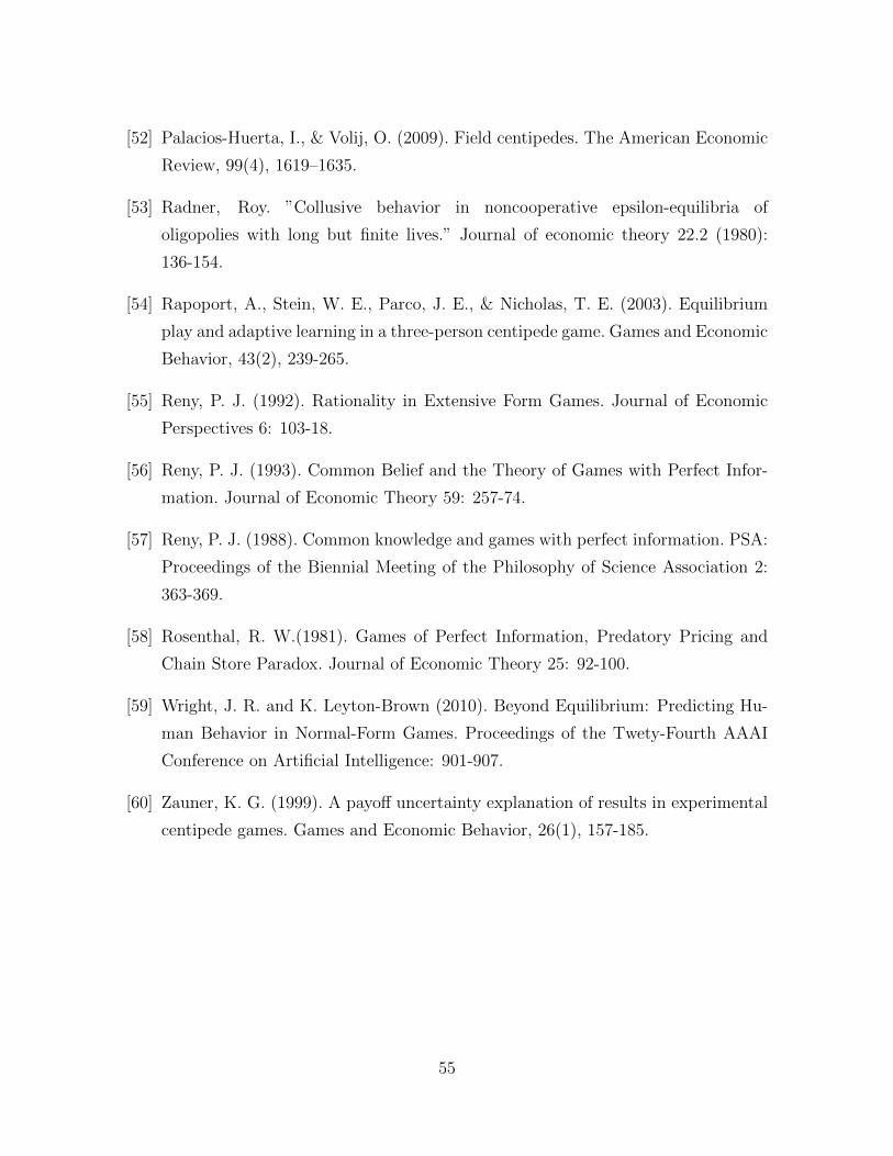
[52] Palacios-Huerta, I., & Volij, O. (2009). Field centipedes. The American Economic

Review, 99(4), 1619–1635.

[53] Radner, Roy. ”Collusive behavior in noncooperative epsilon-equilibria of

oligopolies with long but finite lives.” Journal of economic theory 22.2 (1980):

136-154.

[54] Rapoport, A., Stein, W. E., Parco, J. E., & Nicholas, T. E. (2003). Equilibrium

play and adaptive learning in a three-person centipede game. Games and Economic

Behavior, 43(2), 239-265.

[55] Reny, P. J. (1992). Rationality in Extensive Form Games. Journal of Economic

Perspectives 6: 103-18.

[56] Reny, P. J. (1993). Common Belief and the Theory of Games with Perfect Infor-

mation. Journal of Economic Theory 59: 257-74.

[57] Reny, P. J. (1988). Common knowledge and games with perfect information. PSA:

Proceedings of the Biennial Meeting of the Philosophy of Science Association 2:

363-369.

[58] Rosenthal, R. W.(1981). Games of Perfect Information, Predatory Pricing and

Chain Store Paradox. Journal of Economic Theory 25: 92-100.

[59] Wright, J. R. and K. Leyton-Brown (2010). Beyond Equilibrium: Predicting Hu-

man Behavior in Normal-Form Games. Proceedings of the Twety-Fourth AAAI

Conference on Artificial Intelligence: 901-907.

[60] Zauner, K. G. (1999). A payoff uncertainty explanation of results in experimental

centipede games. Games and Economic Behavior, 26(1), 157-185.

55

Appendix A: Additional Tables and Figures

CG 1 CG 2

CG 3 CG 4

CG 5 CG 6

CG 7 CG 8

Figure A1: Alternative Representation of the Centipede Games used in the Experiment(1-8).

56

CG 9 CG 10

CG 11 CG 12

CG 13 CG 14

CG 15 CG 16

Figure A2: Alternative Representation of the Centipede Games used in the Experiment(9-16).

57

CG 1 CG 2

CG 3 CG 4

CG 5 CG 6

CG 7 CG 8

CG 9 CG 10

CG 11 CG 12

CG 13 CG 14

CG 15 CG 16

Figure A3: The 16 CGs used in the Experiment with the Predictions of the IndividualModels except QRE, A(γ) and IA(ρ, σ) (see Figure A4).

58

CG 1 CG 2

CG 3 CG 4

CG 5 CG 6

CG 7 CG 8

CG 9 CG 10

CG 11 CG 12

CG 13 CG 14

CG 15 CG 16

Figure A4: The 16 CGs Used in the Experiment with the Predictions of QRE, A(γ)and IA(ρ, σ) for the values λ = 0.38, ρ = 0.22 and σ = 0.55.

59

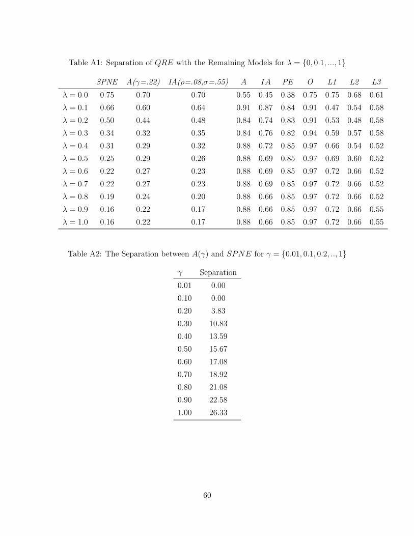
Table A1: Separation of QRE with the Remaining Models for λ = {0, 0.1, ..., 1}

SPNE A(γ=.22) IA(ρ=.08,σ=.55) A IA PE O L1 L2 L3

λ = 0.0 0.75 0.70 0.70 0.55 0.45 0.38 0.75 0.75 0.68 0.61

λ = 0.1 0.66 0.60 0.64 0.91 0.87 0.84 0.91 0.47 0.54 0.58

λ = 0.2 0.50 0.44 0.48 0.84 0.74 0.83 0.91 0.53 0.48 0.58

λ = 0.3 0.34 0.32 0.35 0.84 0.76 0.82 0.94 0.59 0.57 0.58

λ = 0.4 0.31 0.29 0.32 0.88 0.72 0.85 0.97 0.66 0.54 0.52

λ = 0.5 0.25 0.29 0.26 0.88 0.69 0.85 0.97 0.69 0.60 0.52

λ = 0.6 0.22 0.27 0.23 0.88 0.69 0.85 0.97 0.72 0.66 0.52

λ = 0.7 0.22 0.27 0.23 0.88 0.69 0.85 0.97 0.72 0.66 0.52

λ = 0.8 0.19 0.24 0.20 0.88 0.66 0.85 0.97 0.72 0.66 0.52

λ = 0.9 0.16 0.22 0.17 0.88 0.66 0.85 0.97 0.72 0.66 0.55

λ = 1.0 0.16 0.22 0.17 0.88 0.66 0.85 0.97 0.72 0.66 0.55

Table A2: The Separation between A(γ) and SPNE for γ = {0.01, 0.1, 0.2, .., 1}

γ Separation

0.01 0.00

0.10 0.00

0.20 3.83

0.30 10.83

0.40 13.59

0.50 15.67

0.60 17.08

0.70 18.92

0.80 21.08

0.90 22.58

1.00 26.33

60

Table A3: The Separation between IA(ρ, σ) and SPNE for ρ = {0.01, 0.1, 0.2, .., 1}and σ = {0.01, 0.1, 0.2, .., 1}

ρ/σ 0.01 0.10 0.20 0.3 0.40 0.50 0.60 0.70 0.80 0.90 1.00

0.01 0.00 0.00 0.75 1.50 1.50 1.50 1.50 1.50 1.50 1.50 1.50

0.10 0.50 0.50 1.25 1.25 1.25 1.25 1.25 2.00 2.00 2.00 2.00

0.20 3.00 3.17 3.00 3.00 3.00 3.00 3.00 3.00 3.00 3.00 3.00

0.30 5.92 5.75 5.25 5.25 5.25 5.25 5.25 5.25 5.25 5.25 5.25

0.40 7.58 6.92 6.75 6.25 6.25 6.25 6.25 6.25 6.25 6.25 6.25

0.50 10.92 10.17 8.75 8.25 8.25 8.25 8.25 8.25 8.25 8.25 8.25

0.60 12.75 11.00 9.92 9.42 8.42 8.42 8.42 8.42 8.42 8.42 8.42

0.70 19.33 14.25 11.58 11.00 11.00 9.75 9.58 9.58 9.58 9.58 9.58

0.80 20.92 16.08 14.67 12.83 11.58 11.58 11.58 10.25 10.25 10.17 10.17

0.90 21.92 19.58 16.00 14.17 13.17 13.17 11.58 11.58 11.58 10.25 10.25

1.00 21.08 20.75 16.00 14.33 14.33 14.33 13.33 13.33 11.75 11.75 11.75

Separation in Payoffs. This part provides an alternative look at how well the

predictions of the candidate explanations are separated in our CGs, taking into account

the incentives of each behavioral type to behave as a different type. More precisely,

Table A4 compares the incentives of each behavioral type to follow its predictions in

our 16 CGs vs. the predictions of any alternative theory, measured according to the

goal of each type (e.g. the sum of payoffs of both players for A, payoff difference for

IA, and simply payoffs or utilities for the other types). The first row and column list

the different behavioral types; the upper (lower) part of the table corresponds to Player

1(2). A particular cell ij reports the aggregate payoff that the behavioral type in row i

earns in the 16 CGs if she behaves true to type in column j and her opponents behave

in line with the beliefs of type i. In particular, if i = j the cell contains the total payoff

over the 16 CGs of a subject who is of type i always behaves as predicted by rule i and

the opponents always behave according to the beliefs of type i. For example, a Player

1 who adheres to SPNE always ends the game at her first decision node, leading to

8× 40 + 8× 16 = 448 experimental points. For i 6= j, the cells contain the total payoff

in the 16 CGs that type i obtains if she keeps the beliefs of type i but behaves as type

j instead. As example, consider a SPNE player with SPNE beliefs who behaves as

A. Since such a player expects the opponent to behave according to SPNE, the cell

61

(SPNE,A) contains 20 + 10 + 20 + 10 + 2 + 1 + 38 + 1 + 13 + 15.25 + 40 + 16 +

33 + 11 + 10 + 39.25 = 279.5. Note that no such analysis can be carried out for PE

as they are not following an optimization problem, although it is possible to calculate

the payoff that other behavioral types would earn if they followed the PE prescription

rather than their own optimal strategy.

Table A4: Separation in Payoffs between Different Models

Player 1SPNE A(γ) IA(ρ,σ) A IA PE O L1 L2 L3 QRE(λ = 0.38)

SPNE 448.00 434.67 448.00 279.50 368.00 280.33 271.00 354.00 329.00 366.00 380.41A(γ=.22) 492.82 655.28 492.82 681.26 490.62 684.13 673.95 733.67 633.42 732.46 618.81

IA(ρ=.08,σ=.55) 429.34 368.06 429.34 45.11 352.50 44.35 31.12 181.97 181.91 202.36 264.52A 656.00 1856.67 656.00 6859.00 831.67 6827.42 6856.00 6408.00 2165.00 2191.00 1403.06IA 240.00 323.33 240.00 436.50 141.00 447.42 427.00 397.00 424.00 415.00 366.31O 448.00 1423.33 448.00 5283.28 587.00 5258.69 5307.20 5133.00 1571.00 1703.00 1065.40L1 448.00 796.25 448.00 1781.78 484.08 1783.61 1755.95 1861.75 1028.00 1122.00 776.19L2 448.00 664.67 448.00 851.25 383.00 863.75 830.00 902.00 1571.00 1542.00 1 816.95L3 448.00 729.33 448.00 1011.13 495.25 1024.08 992.50 1034.00 1539.50 1703.00 910.26

QRE(λ = 0.38) 448.00 539.28 448.00 466.69 437.23 472.25 443.48 512.85 517.39 541.97 553.37

Player 2SPNE A(γ) IA(ρ,σ) A IA PE O L1 L2 L3 QRE(λ = 0.38)

SPNE 208.00 208.00 208.00 208.00 208.00 208.00 208.00 208.00 208.00 208.00 208.00A(γ) 381.00 580.72 381.00 740.04 572.11 740.04 740.04 744.56 756.49 462.75 490.55

IA(ρ,σ) 76.25 76.25 76.25 76.25 76.25 76.25 76.25 76.25 76.25 76.25 76.25A 876.00 1436.00 991.75 6859.00 3302.50 5432.33 4037.00 3685.00 3771.75 1557.75 1480.50IA 218.00 215.67 201.50 189.75 141.00 181.75 158.00 159.00 187.00 191.50 184.71O 595.00 962.17 680.75 1661.10 1635.27 2304.93 3009.20 2847.00 2774.75 1031.60 1029.40L1 498.25 592.83 526.50 700.04 740.45 860.08 1027.33 1106.25 1054.00 662.54 632.86L2 487.00 853.17 487 1284.25 1278.50 1806.08 2299.00 2565.00 2584.00 840.00 773.69L3 499.00 531.00 536.75 584.00 621.58 591.67 581.00 581.00 582.75 942.00 700.51

QRE(λ = 0.38) 396.19 401.73 409.12 346.52 377.21 347.05 330.05 335.18 412.13 384.42 427.23

By construction, the comparison of the i = j values with i 6= j illustrate the

incentives of a subject of a particular type to comply or not with her type. In the

table, the highest values (lowest payoff difference for IA) are in bold. As expected,

almost all types maximize their goal if they follow the prescriptions of their type, while

alternative decision rules typically yield a lower payoff (higher payoff difference in case

of IA).52 The behavioral types that show the widest separation in payoffs is those of A

and O, while SPNE and QRE show the smallest separation.

Replication of Behavior. Compared to earlier experimental studies on CGs,

we have changed several features in the procedures in carrying out our experiment.

First and most importantly, we apply the strategy method rather than the direct hot-

hand method. Second, our subjects played several CGs and we only elicit the initial

responses in each game. Third, we only pay for three randomly chosen games. As a

result, we first ask whether these features do not distort subjects’ behavior vis-a-vis

52If Player 1 behaves according to SPNE Player 2’s behavior is irrelevant. Hence, the 208 experi-mental points in all columns for SPNE -Player 2.

62

other studies.

Exponentially Increasing-sum Constant-sum

Figure A5: Comparison of Behavior across Different Studies

Our exponentially increasing-sum CG 1 belongs to the most commonly tested varia-

tions of CGs. We compare the behavior of our 151 subjects who played the no-feedback,

cold version of the game with three other studies. First, we contrast their behavior with

the initial lab behavior of students in Palacios-Huerta and Volij (2009). Their subjects

(like ours) came from the University of the Basque Country. There were 80 students

(40 in each role, as opposed to our 151, 76 as Player 1 and 75 as Player 2) and none

of their students came from Economics or Business (whereas ours mostly come from

these two fields). Second, we also compare our subjects’ behavior with those of the 58

subjects (29 in each player role) in McKelvey and Palfrey (1992). Third, we contrast

our data with the obtained in Kawagoe and Takizawa (2012). They do not report the

exact number of subjects; we approximate it from the information on the number of

sessions and participants in each session. Given the different elicitation methods, we

cannot directly compare the behavior. To be able to compare them, we create 100,000

random sub-samples from our data to match the number of subjects in Palacios-Huerta

and Volij (2009) and McKelvey and Palfrey (1992), and the approximate number of

subjects in Kagawoe and Takizawa (2012), respectively. For each sub-sample, we ran-

domly pair Players 1 and 2 and record the behavior that we would observe if these two

individuals interacted. Each of the 100,000 sub-samples thus generates one possible

distribution of behavior if our subjects participated in an experiment under the condi-

tions of the studies in the comparison. The white bars in Figure A5, on the left, report

the average simulated stopping frequencies at a particular decision node in the 100,000

63

simulated sub-samples corresponding to the conditions of Palacios-Huerta and Volij

(2009). The black and grey bars show the observed stopping frequencies in Palacios-

Huerta and Volij (2009), McKelvey and Palfrey (1992), and Kawagoe and Takizawa

(2012), in this order. The horizontal bars present the 95% percentiles of the simulated

distributions of behavior under Palacios-Huerta and Volij (2009)’s conditions.53 It can

be seen that the behavior in our experiment is relatively similar to that in the study

by to Palacios-Huerta and Volij (2009). When it differs, it typically deviates towards

the frequencies observed in McKelvey and Palfrey (1992) or Kawagoe and Takizawa

(2012), where there is a general tendency to stop somewhat later.

The right-hand side of Figure A5 also compares the corresponding simulated be-

havior in CG 9 with the initial behavior of the 58 subjects in Fey et al. (1996) and

the behavior of the 40-48 (approximated by 44) subjects presented in Kawagoe and

Takizawa (2012). The behavior is very similar in all cases.

We thus conclude that the behavior in our CG 1 and 9 is comparable to that of

other studies.54 In CG 1, our observed behavior is particularly close to the one observed

in the experiment by Palacios-Huerta and Volij (2009), conducted few years earlier at

the same University; in CG 9, our observed behavior is very close to both Fey et al.

(1996) and Kawagoe and Takizawa (2012). Hence, our design features do not seem to

distort subjects’ behavior.

53For the sake of readability, we omit the corresponding simulated behavior for McKelvey andPalfrey’s (1992) and Kawagoe and Takizawa (2012) conditions in the figure and only use them for thestatistical tests below. Since there are more observations in Palacios-Huerta and Volij (2009), theirconditions generate less variability in the simulated behavior and thus present a more conservativecomparison.

54We performed Pearson chi-square tests of independence with two alternative null hypotheses.First, the test of the null hypothesis that the simulated play of different ending nodes in our experimentis not different from the behavior in other studies yields p-values of 0.38, 0.34, 0.64, 0.00 and 0.56 for thecomparison with Palacios-Huerta and Volij (2009), McKelvey and Palfrey (1992), Fey et al. (1996),and the increasing- and constant-sum treatments of Kawagoe and Takizawa (2012), respectively.Second, the test of the null hypothesis that the behavior from other studies come from our simulatedplay yields p-values of 0.09, 0.07, 0.49, 0.00 and 0.35 respectively. No test is rejected at conventional5% significance, with the exception of the increasing-sum treatment of Kawagoe and Takizawa (2012)where subjects stop significantly later than in our and the other studies. Since this difference alsoarises in the comparison of Kawagoe and Takizawa (2012) with McKelvey and Palfrey (1992) andPalacios-Huerta and Volij (2009), we conclude that the behavior of our subjects does not differ fromthat in other studies.

64

CG 1 CG 2

CG 3 CG 4

CG 5 CG 6

CG 7 CG 8

Figure A6: Observed Aggregate Behavior in CGs 1-8.

65

CG 9 CG 10

CG 11 CG 12

CG 13 CG 14

CG 15 CG 16

Figure A7: Observed Aggregate Behavior in CGs 9-16.

66

Table A5: Consistency for Different Criteria (Each cell shows the number of subjects(out of 151) who comply with a behavioral model in the corresponding column in acertain number of CGs or more, defined in the first column)

SPNE A(γ=.22) IA(ρ=.08,σ=.55) A IA PE O L1 L2 L3 QRE(0.38)

0 151 151 151 151 151 151 151 151 151 151 151

1 142 144 142 150 147 151 124 151 149 149 151

2 139 141 139 95 133 124 92 150 148 138 149

3 128 127 127 54 117 78 57 148 145 128 142

4 108 113 108 25 63 35 39 134 136 117 129

5 96 95 94 13 32 10 33 116 123 101 96

6 79 80 77 8 12 7 19 100 110 81 77

7 65 64 62 6 5 3 14 79 85 63 48

8 49 50 47 5 2 3 8 61 53 46 19

9 39 38 36 4 0 2 6 34 24 30 4

10 29 26 26 3 0 2 4 26 9 16 0

11 19 16 17 2 0 0 4 15 4 5 0

12 12 7 12 0 0 0 4 5 2 1 0

13 6 2 5 0 0 0 4 3 0 0 0

14 4 1 2 0 0 0 3 1 0 0 0

15 1 0 0 0 0 0 3 0 0 0 0

16 1 0 0 0 0 0 3 0 0 0 0

Table A6: Estimation Results with two QRE types.

Original Results Two QREType pk εk, λ pk εk, λ

SPNE 0.08 0.31 0.09 0.06O 0.03 0.06 0.03 0.60L1 0.31 0.60 0.31 0.66L2 0.21 0.66 0.21 0.62L3 0.11 0.62 0.10 0.76

QRE 1 0.27 0.42 0.22 0.38QRE 2 0.06 0.32

67

0 0.2 0.4 0.6 0.8 10

0.2

0.4

0.6

0.8

1

QRE

0 0.2 0.4 0.6 0.8 10

0.2

0.4

0.6

0.8

1

SPNE

0 0.2 0.4 0.6 0.8 10

0.2

0.4

0.6

0.8

1

Optimistic

0 0.2 0.4 0.6 0.8 10

0.2

0.4

0.6

0.8

1

Level-k

Figure A8: Distribution of per-subject Posterior Probabilities of Belonging to EachModel, Computed for the Reduced Model with the Uniform-error Specification (3-4) in Table 6A. The table shows that a vast majority of subjects is classified withprobability close to 1 to one unique rule, suggesting a clean segregation of behavioraltypes in our data.

68

Table A7: Estimations with 15 in-sample Games. Out-sample CGs 1-8.

Out-sample CGType 1 2 3 4 5 6 7 8

SPNE (pk) 0.10 0.07 0.09 0.09 0.07 0.08 0.09 0.09(0.04) (0.03) (0.03) (0.03) (0.03) (0.03) (0.03) (0.03)

O (pk) 0.03 0.03 0.03 0.03 0.03 0.03 0.03 0.03(0.01) (0.01) (0.01) (0.01) (0.01) (0.01) (0.01) (0.01)

L1 (pk) 0.30 0.31 0.31 0.34 0.30 0.29 0.25 0.31(0.06) (0.06) (0.06) (0.06) (0.06) (0.05) (0.05) (0.06)

L2 (pk) 0.13 0.20 0.17 0.18 0.26 0.25 0.22 0.19(0.06) (0.06) (0.06) (0.05) (0.07) (0.06) (0.05) (0.05)

L3 (pk) 0.08 0.12 0.09 0.09 0.09 0.05 0.03 0.15(0.05) (0.05) (0.05) (0.05) (0.04) (0.04) (0.04) (0.06)

QRE (pk) 0.36 0.27 0.30 0.28 0.25 0.31 0.39 0.24(0.05) (0.05) (0.05) (0.04) (0.05) (0.05) (0.06) (0.05)

SPNE (εk) 0.31 0.24 0.35 0.33 0.26 0.27 0.33 0.33(0.09) (0.14) (0.08) (0.08) (0.07) (0.06) (0.07) (0.09)

O (εk) 0.07 0.07 0.07 0.07 0.07 0.07 0.07 0.07(0.13) (0.09) (0.10) (0.14) (0.11) (0.08) (0.14) (0.14)

L1 (εk) 0.60 0.60 0.61 0.65 0.60 0.58 0.57 0.59(0.04) (0.10) (0.04) (0.04) (0.05) (0.05) (0.05) (0.04)

L2 (εk) 0.60 0.65 0.68 0.63 0.59 0.60 0.64 0.66(0.11) (0.17) (0.12) (0.05) (0.05) (0.05) (0.08) (0.12)

L3 (εk) 0.89 0.62 0.62 0.65 0.79 0.92 0.99 0.58(0.17) (0.05) (0.15) (0.13) (0.17) (0.18) (0.19) (0.10)

QRE (λ) 0.32 0.43 0.41 0.43 0.44 0.38 0.25 0.42(0.09) (0.08) (0.07) (0.11) (0.11) (0.09) (0.08) (0.14)

69

Table A8: Estimations with 15 in-sample Games. Out-sample CGs 9-16

Out-sample gameType 9 10 11 12 13 14 15 16

SPNE (pk) 0.08 .011 0.09 0.09 0.07 0.07 0.04 0.08(0.04) (0.03) (0.03) (0.03) (0.03) (0.03) (0.03) (0.03)

O (pk) 0.03 0.03 0.03 0.03 0.03 0.03 0.03 0.03(0.01) (0.01) (0.01) (0.01) (0.01) (0.01) (0.01) (0.01)

L1 (pk) 0.28 0.33 0.30 0.30 0.30 0.34 0.29 0.30(0.05) (0.05) (0.05) (0.05) (0.05) (0.06) (0.05) (0.05)

L2 (pk) 0.23 0.18 0.21 0.18 0.21 0.20 0.25 0.23(0.07) (0.06) (0.06) (0.06) (0.07) (0.07) (0.06) (0.06)

L3 (pk) 0.14 0.05 0.03 0.10 0.15 0.10 0.15 0.10(0.06) (0.04) (0.04) (0.05) (0.05) (0.05) (0.06) (0.05)

QRE (pk) 0.25 0.30 0.35 0.30 0.24 0.27 0.23 0.26(0.05) (0.06) (0.05) (0.05) (0.05) (0.05) (0.06) (0.05)

SPNE (εk) 0.32 0.32 0.34 0.34 0.29 0.30 0.19 0.31(0.10) (0.06) (0.08) (0.09) (0.08) (0.07) (0.11) (0.11)

O (εk) 0.07 0.07 0.05 0.04 0.07 0.07 0.05 0.07(0.10) (0.10) (0.15) (0.15) (0.20) (0.16) (0.11) (0.13)

L1 (εk) 0.59 0.62 0.60 0.60 0.59 0.62 0.61 0.56(0.04) (0.05) (0.04) (0.04) (0.04) (0.04) (0.04) (0.04)

L2 (εk) 0.65 0.66 0.65 0.66 0.62 0.63 0.66 0.69(0.09) (0.09) (0.06) (0.06) (0.08) (0.08) (0.06) (0.08)

L3 (εk) 0.58 0.61 0.99 0.69 0.60 0.59 0.65 0.55(0.12) (0.16) (0.15) (0.12) (0.12) (0.15) (0.08) (0.11)

QRE (λ) 0.43 0.26 0.26 0.27 0.43 0.42 0.58 0.38(0.15) (0.10) (0.10) (0.13) (0.14) (0.14) (0.14) (0.12)

70

Table A9: The Percentual Improvement of the Log-likelihoods Explaining Behaviorout-of-sample, with respect to Random Behavior. Each column corresponds to one out-of-sample game; the rows list the different models. Level-k corresponds to a mixtureof L1, L2, and L3.

Game predicted1 2 3 4 5 6 7 8 9 10

Mixture 0.05 0.12 0.05 0.13 0.13 0.04 0.10 0.11 0.17 0.15QRE -0.60 -1.00 -0.06 0.17 0.13 -0.08 -0.22 0.13 0.19 0.15SPNE -0.10 -0.14 -0.04 -0.04 0.05 0.00 0.02 0.09 0.05 -0.05O 0.00 0.00 0.00 0.00 0.00 0.00 0.00 0.00 0.00 0.00Lk 0.04 0.05 0.07 0.10 0.08 0.06 0.03 0.04 0.21 0.14

11 12 13 14 15 16 Mean St.dev. St.Er.Mixture 0.18 0.22 0.09 0.08 0.24 0.13 0.12 0.06 0.01QRE 0.09 0.18 0.11 0.08 0.32 0.12 -0.02 0.34 0.08SPNE 0.14 0.12 0.05 0.01 0.15 0.05 0.02 0.08 0.02O 0.00 0.00 0.00 0.00 0.00 0.00 0.00 0.00 0.00Lk 0.18 0.22 -0.10 -0.04 0.28 0.03 0.09 0.10 0.02

Appendix B: Instructions in English (original in Spanish)

THANK YOU FOR PARTICIPATING IN OUR EXPERIMENT!

This is an experiment, so there is to be no talking, looking at what other participants

are doing or walking around the room. Please, turn off your phone. If you have any

questions or you need help, please raise your hand and one of the researchers will

assist you. Please, do not write on these instructions. If you fail to follow these rules,

YOU WILL BE ASKED TO LEAVE THE EXPERIMENT AND YOU WILL NOT

BE PAID. Thank you.

The University of the Basque Country has provided the funds for this experiment.

You will receive 3 Euros for arriving on time. Additionally, if you follow the instructions

correctly you have the chance of earning more money. This is a group experiment.

Different participants may earn different amounts. How much you can win depends on

your own choices, on other participants choices, and on chance.

No participant can identify any other participant by his/her decisions or earnings

in the experiment. The researchers can observe each participant earnings, but they

will not associate your decisions with the name of participant name.

During the experiment you can win experimental points. At the end, these exper-

imental points will be converted into cash at a rate of 1 experimental point = 0.05

euros. Everything you earn will be paid in cash, in a strictly private way at the end of

71

the experimental session.

Your final earnings will be the sum of the 3 Euros that you get just for participating

and the amount that you earn during the experiment.

Each experimental point earns you 5 Euro cents, so 20 experimental points make 1

euro (20 x 0,05 = 1 Euro).

For example, if you obtain a total of 160 experimental points you will earn a total

of 11 Euros (3 for participating plus 8 from converting the 160 experimental points

into cash).


of 7.5 Euros (90 x 0.05 = 4.5 + 3 = 7.5)


of 22 euros (380 x 0.05 = 19 + 3 = 22)

Groups:

All participants in these sessions will be randomly divided in two different groups,

the RED group and the BLUE group. Before you start making decisions, you will

be informed if you are RED or BLUE, and you will maintain that status throughout

the experiment. Each participant in the RED group will be randomly matched with a

BLUE participant.

Game and options:

The experiment will consist of 16 games. In each game you will be matched ran-

domly with a participant form other group. Nobody will know the identity of the

participant with whom you are matched, nor will it be possible to identify him/her by

his/her decisions during or after the experiment.

A description of the games follows. Every game has the same format, as represented

in graphic form below.

If you are a RED participant, you will see this version of the game, where you can

choose between the red circles only.

If you are a BLUE participant, you will see this other version of the game, where

you can choose between the blue circles only.

In each game, each participant, RED or BLUE, has three chances to determine

the earnings of both participants, in which he/she can one of two actions: stop or

continue. In the graphic representation, the circles colored, RED and BLUE, identify

which participant chooses. As the direction of the arrows shows, the game should

72

Figure A9: ROJO

Figure A10: AZUL

be read from left to right. The earnings of the two participants are represented by

X and Y, which in each circle of each game will be different numbers, representing

experimental points.

The RED participant has the first chance to choose: he/she can “Stop here” or

continue. In the graphic representation the downward arrow in the first RED circle

represents “Stop” and the rightward arrow represents continue. If the RED participant

chooses “Stop here”, the RED participant receives X1 and the BLUE participant Y1,

and the game ends. If the RED participant does not choose “Stop here”, then the

game continues and it is the BLUE participant who chooses in the first blue circle.

The BLUE participant can choose “Stop” or continue. In the graphic represen-

tation, the downward arrow in the first BLUE circle represents “Stop here” and the

rightward arrow represents continue. If the BLUE participant chooses “Stop here” the

RED participant receives X2 and the BLUE participant Y2, and the game ends. If the

BLUE participant does not choose “Stop here”, then the game continues and it is the

RED participant who chooses again in the second red circle

This description is repeated in the second red and blue circles, until the last chance

is reached by the RED and BLUE participants.

In the last chance for the RED participant, represented by the third and last red

circle, the RED participant can choose “Stop here” or “Never stop”. If the RED partic-

ipant chooses “Stop here” the RED participant receives X5 and the BLUE participant

73

Y5, and the game ends. If the RED participant chooses “Never stop”, then it is the

BLUE participant who chooses for the last time.

In the last chance for the BLUE participant, represented by the third and last blue

circle, the game ends. If the BLUE participant chooses ”Stop here” each participant

receives, X6 for the RED and Y6 for the BLUE, and the game ends. If the BLUE

participant chooses “Never stop” the game ends and the quantities that the participants

receive are X7 for the RED and Y7 for the BLUE.

In summary, in each game you have to choose where to stop or whether not to stop.

That means that in each game you can choose between four different options: stop in

the first circle of your color, stop in the second circle of your color, stop in the third

circle of your color, or “Never stop”. The quantities change on each occasion and the

participant who chooses “Stop here” before the other participant is the one who ends

the game and determines the experimental points earned by both participants.

In order to make the game easier to understand, three examples are shown below.

In the examples we show a choice by the RED participant (shaded in red) and one by

the BLUE (shaded in blue) for a hypothetical game, and we identify the earnings for

each participant.

Example 1:

Figure A11: Ejemplo 1(ROJO)

Figure A12: Ejemplo 1(AZUL)

The RED participant has chosen “Stop”in the first red circle and the BLUE par-

74

ticipant has chosen “Stop”in the first blue circle. Because the RED participant has

stopped before the BLUE participant:

The RED participant earns: 40

The BLUE participant earns: 10

Example 2:



The RED participant has chosen “Stop”in the second red circle and the BLUE

participant has chosen “Never stop”. Because the RED participant has stopped before

the BLUE participant:



Example 3:


The RED participant has chosen “Never stop” and the BLUE participant has chosen

stop in the third blue circle. Because the BLUE participant has stopped before the

RED participant:

75




Note: These examples are just an illustration. The experimental points that appear

are examples, i.e. they are not necessarily the ones that will appear in the 16 games.

In addition, the examples ARE NOT intended to suggest how anyone should choose

between the different options.

How the computer works: In each game, you will see 4 white boxes, one for each

of your possible options. To choose an option, click on the corresponding box. When

you have selected an option, the box will change color, as shown in the examples. This

choice is not final: you can change it whenever you want by clicking on other box as

long as you have not yet clicked the “OK” button that will appear in the bottom-left

corner of each screen. Once you click “OK” your choice will be final and you will move

on to the next game. You cannot pass on to the next game until you have chosen an

option and have clicked “OK”.

Earnings:

Once you have submitted your choices in the 16 games, the computer chooses three

games at random for each participant for payment. You will be paid depending on the

actions that you chose and the ones that the participant you were matched with chose

in each of those three games.

Summary:

• The computer will choose randomly whether you are a RED or BLUE participant

for the whole experiment.

• You will participate in 16 different games and in each of them you will be matched

randomly with a participant of the other color.

• In each game, each participant can choose between four different options: stop in

the first circle of his/her color, stop in the second circle of his/her color, stop in

76

the third circle of his/her color or “Never stop”. The quantities change on each

occasion and the participant that chooses “Stop here” before the other participant

is the one that ends the game and determines the experimental points for both

participants.

• At the end, the computer will randomly choose 3 of the 16 games for each player,

and you will be paid depending on the actions chosen by you and by the partic-

ipant you were matched to in each of those three games.

The experiment will start shortly. If you have any questions or you need help,

please, raise your hand and one of the researchers will help you.

77

non-equilibrium play in centipede games · 1 introduction the centipede game (cg, hereafter),...

Documents