experimental results on the centipede game in normal form: an

Journal of Mathematical Psychology 42, 356�384 (1998)

Experimental Results on the Centipede Game inNormal Form: An Investigation on Learning

Rosemarie Nagel*

Department of Economics, Universitat Pompeu Fabra, Barcelona, SpainE-mail: nagel�upf.es

and

Fang Fang Tang

Department of Economics and Statistics, National University of Singapore,E-mail: ecstff�nus.edu.sg

We analyze behavior of an experiment on the centipede game played in thereduced normal form. In this game two players decide simultaneously whento split a pie which increases over time. The subjects repeat this game 100times against randomly chosen opponents. We compare several static modelsand quantitative learning models, among them a quantal response, modelreinforcement models and fictitious play. Furthermore, we structure behaviorfrom period to period according to a simple cognitive process, called learningdirection theory. We show that there is a significant difference in behaviorfrom period to period whether a player has decided to split the pie before orafter the opponent. � 1998 Academic Press

INTRODUCTION

In this study, we report experimental results on centipede games in reducednormal form, played repeatedly against changing opponents. The main purpose ofthis study is to compare different learning models. Originally, the centipede game

Article No. MP981225

3560022-2496�98 �25.00Copyright � 1998 by Academic PressAll rights of reproduction in any form reserved.

* Corresponding author: Rosemarie Nagel, Department of Economics, Universitat Pompeu Fabra,Ramon Trias Fargas 24-27, 08005 Barcelona, Spain, E-mail: nagel�upf.es. We thank Antonio Cabrales,Colin Camerer, Gary Charness, Ido Erev, Nick Feltovitch, Michael Mitzkewitz, Alvin Roth, AbdolkarimSadrieh, Reinhard Selten, and two anonymous referees for helpful comments, Tibor Neugebauer forproviding his computerprogram for this experiment and organizing the experiments. Special thanks alsoto the Bonn Laboratorium fuer experimentelle Wirtschaftsforschung for their support running theexperiments. We thank Serguei Maliar and Nick Feltovitch for providing parts of the simulations andRichard McKelvey for the computations of the quantal response equilibria. Financial support fromthe German Science Foundation through SFB303 (University of Bonn) to Nagel and Tang and thepostdoctoral fellowship of the University of Pittsburgh to Nagel are gratefully acknowledged.

(Rosenthal, 1981) has been discussed mainly in extensive form in the theoretic andexperimental literature. The game in extensive form is as follows (see also Fig. 1):two players, called player A and player B, decide sequentially whether to split agiven pie in a predetermined way or whether to pass the splitting option to theother player. If a player passes the decision to the other player, the pie increases insize. Passing can be done only a finite number of times. Once a player splits the pie,the game is over with that player gaining the higher share of the pie and the otherplayer obtaining the smaller share. All standard game-theoretic equilibriumconcepts predict that the pie is split at the first decision node of player A, the firstplayer.

In the reduced normal form game, which is strategically equivalent to the extensiveform game, players decide simultaneously at which of his decision nodes to ``take''the opportunity to split the pie. This form of decision making has an advantage forstudying learning in centipede games. The experimenter is informed about theintended ``Take-node'' by both players. Thus, in the repeated normal form gameswe are able to study the change of behavior of a player from round to round in amore precise way than can be done in the extensive form game. Furthermore, thiskind of structure allows us to repeat long centipede games much faster than repeatedsequential move games. However, while there might be substantial differences inbehavior in the extensive form game and in the normal form game, we do notaddress this question here and leave that to a later study. Here we only concentrateon learning in the normal form game. Since after each period the players onlyobtain information as in the extensive form game, we hope that the structure ofbehavior we find will be valuable for the understanding of behavior in the extensiveform centipede games. The centipede game in extensive form has gained attentionin game theory in the discussion on the limitations of common knowledge ofrationality and backward induction (see, e.g., Aumann, 1992; Binmore, 1988).Cressman and Schlag (1996) and Ponti (1996) discuss stability criteria of anevolutionary model in the centipede game.

McKelvey and Palfrey (1992), Fey, McKelvey, and Palfrey (1994), Zauner(1996), and McKelvey and Palfrey (1995b) have analyzed actual behavior in theextensive-form centipede game. As in our experiments, behavior is quite differentfrom the game theoretic solution. These authors explain the data in terms of equili-brium models with errors. Learning is discussed as reduction of errors or reductionof uncertainty over time. As a consequence of that kind of learning, behavior shouldconverge to the Nash-equilibrium of the stage game. We apply the quantal responsemodel (McKelvey 6 Palfrey, 1995a) for our data set and compare it with othermodels, some static models, a class of simple adaptive models, called reinforcementlearning models, and fictitious play. Furthermore, we formulate hypotheses accordingto a qualitative learning direction model, in the spirit of Selten and Stoecker (1986).Testing these hypotheses we reveal features of period to period behavior that havenot been discussed in other studies on the centipede game. There seems to be aclear-cut separation of behavior whether a player has chosen the lower number orhas chosen the higher number of the match. Learning is not necessarily related toconvergence to equilibrium. All models we consider have been applied by differentauthors to various experimental games in the economic literature.

357RESULTS ON THE CENTIPEDE GAME

The paper is organized as follows. Section 2 presents the game under considera-tion and Section 3 the experimental design. Section 4 gives a summary statistic ofthe data. Section 5 discusses quantitative static models and learning models andcompares the performance of these models in the light of the data. Section 6 analysesthe actual data and the basic reinforcement model with respect to hypotheses of aqualitative learning theory��learning direction theory. Section 7 concludes.

1. THE GAME UNDER CONSIDERATION

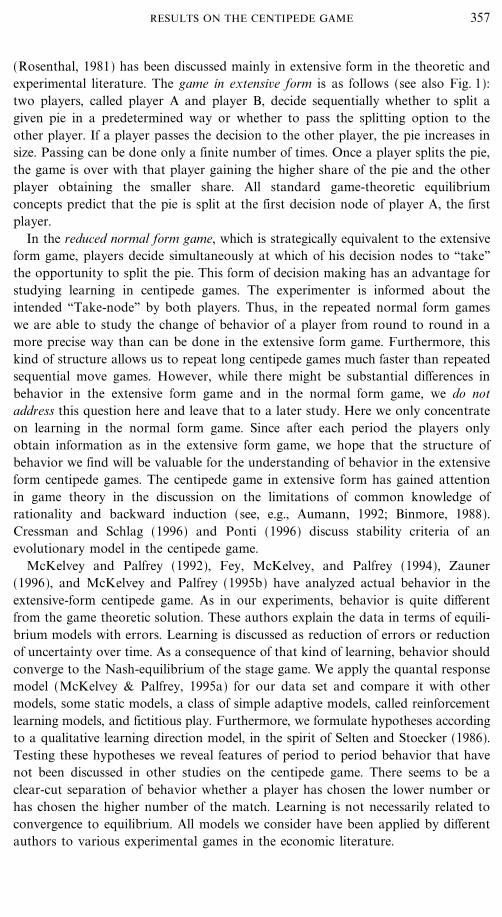
Consider the extensive form game displayed in Fig. 1. At each node (numberedfrom 1 to 12) either player A or player B has to decide whether to ``take'' or to``pass.'' Once a player chooses ``take,'' the game is over and the payoffs are deter-mined by the payoff vector at that ``Take-node.''

FIG. 1. The centipede game in extensive game form (*=Nash-equilibrium payoffs).

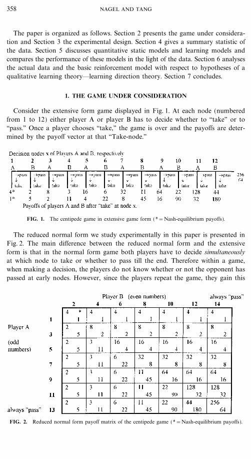
The reduced normal form we study experimentally in this paper is presented inFig. 2. The main difference between the reduced normal form and the extensiveform is that in the normal form game both players have to decide simultaneouslyat which node to take or whether to pass till the end. Therefore within a game,when making a decision, the players do not know whether or not the opponent haspassed at early nodes. However, since the players repeat the game, they gain this

FIG. 2. Reduced normal form payoff matrix of the centipede game (*=Nash-equilibrium payoffs).

358 NAGEL AND TANG

experience from game to game instead within a game. The simultaneity removesany explicit sequential ``reciprocity.'' If a player played repeatedly against the sameopponent, there could be reciprocity from period to period.

The strategies : (for the row (A)-player are odd numbers between 1 and 13,: # [1, 3, ..., 13]; and the strategies ; for the column (B)-player are even numbersbetween 2 and 14, ; # [2, 4, ..., 14]; numbers 1 to 12 indicate the take node of theextensive form. Strategies 13 and 14 correspond to the strategy ``always pass'' in theextensive form, resulting in the highest payoff for player A.1 Since some cellscontain the same payoff vectors, players cannot always infer what an opponent haschosen; in the extensive form game, a player who takes before his opponent, doesnot know opponent's move, except at node 12. We maintain this information of theextensive form game by not telling the subjects what the other player has done ifhe cannot infer it from the matrix.

Both games are strategically equivalent and have a unique outcome. In the exten-sive form game, the players have to take at their first opportunity following thebackward induction logic. The equilibrium is subgame-perfect. There are also mixedequilibria with the same outcome, player A ``takes'' the first node and player Bmixes between later nodes with a positive probability such that player A has noreason to deviate from his strategy. In the normal form game, the players choosestrategy 1 and 2, respectively. There is only one form of elimination process toreach this equilibrium2: Strategy 14 is a weakly dominated strategy (see normalform payoffs for player B). Thus, player B will not play 14. If player A believes that,he can delete 13, assuming that player B is rational. Then, player B should eliminate12 and so on. This process is called iterative elimination of weakly dominated strategieswith strategies 1 and 2 being singled out. However, always ``passing'' by both playersor player A always ``passing'' and player B taking strategy 12 (taking at the last node)are the Pareto optimal strategy combination. If the game is finitely repeated against thesame opponent or repeated against changing opponents, the pure one shot equilibriumis maintained and there are no other pure equilibria.

2. EXPERIMENTAL DESIGN

We ran five sessions of the centipede game in reduced normal form with payoffsas shown in Fig. 2. Both the first endnode and the last endnode have the samepayoff vector as in the 6-move game in McKelvey and Palfrey (1992). Each playerhas seven choices; player A chooses an odd number from 1 to 13 and player B aneven number from 2 to 14.3 Each session involved 12 subjects (six for type A and


1 In the nonreduced normal form game, a player has to decide for each of his node whether to takeor to pass. This is according to the definition of a strategy in the extensive form game, allowing for anenormously large strategy space. However, all strategies with the same first intended Take node producethe same payoff. Passes at later nodes have no influence on the outcome. McKelvey and Palfrey runpilot studies on the nonreduced normal form. More than 950 of the chosen strategies were monotonicin Take behavior, i.e., after the first intended Take node all other nodes were followed by a Take.

2 See also Glazer and Rubinstein (1996) who discuss the equivalence of solving normal form andextensive form games.

3 We also ran five sessions of a game with four actions for each player, with the same payoff structureas in the 6-move game of McKelvey and Palfrey (1992). We will not discuss the results here.

six for type B) from various departments of the University of Bonn. Each subjectparticipated only in one session maintaining the same role throughout the session.The interaction between subjects was via computer terminals. After the assistanthad read the instructions aloud (see Appendix), subjects were randomly allocatedto one of the two types (type A or type B). Subjects were informed that the sameone-shot game was repeated for 100 periods and in each period, a player of onetype was randomly matched with a player from the other type without identifyingthe players to each other. Instead of displaying the normal form, we presented andexplained a table as shown in the instructions (see Appendix): The lower number(column 1) of a matched pair determines the payoff for each player, which is shownin column 3 for player A and column 4 for player B. Since 14 can never be thelower node, it is not shown in the table. Column 2 presents the possible choicesof the opponent in case he chooses the higher number. For example, if the lowernumber is 9, player A must have chosen it, and player B has chosen either 10, 12,or 14. This way we reduce the normal form to the diagonal cells and one cell ofeach row below the diagonal. In the last column the total sum of the pie is stated.We additionally mentioned that the pie increases by about 400 with each increasinglower number. The person who chooses the lower number of the match receives about800 of the pie.

During a session, columns 1, 3, and 4 of the table in the instructions were alwaysdisplayed on the screen. Player A had seven colored buttons numbered 1, 3,..., 13 tochoose from by clicking one button with the mouse or pressing the number on thekeyboard. The choices from player B were also displayed as gray buttons, withno consequence if pressed by a mouse button. Player B screen was similar withnumbers 2, 4,..., 14 as colored buttons.

After each round, each player is informed of the lower number of his match (thishe can also infer from the payoffs), the corresponding payoffs to both players, andhis own cumulative payoff. Thus, the player who chooses the lower number is notinformed about the choice of the opponent, as in the centipede game in extensiveform. During the session their own complete history was displayed if requested bya mouse click.4

At the end of a session the total points were converted into DM (2 points=0.01DM), and paid privately to each subject. Each session lasted about 1 to 1 1�2 h.Average payoffs were 17.70 DM (about 812.60). Note that the sessions by M�P(1992) who repeated each six-move game 10 periods took also 1 h.

3. POOLED RESULTS

Many patterns of the behavior found in the extensive form game study byMcKelvey and Palfrey (M�P, 1992) and repeated in Zauner (1996) can also berecognized in our study. Table I shows the relative frequencies of choices of playersA and B for each session.

360 NAGEL AND TANG

4 Subjects examined their history about 60 of the time, both in the first 50 periods and the last 50periods.

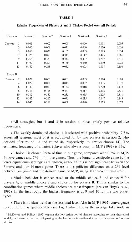
TABLE I

Relative Frequencies of Players A and B Choices Pooled over All Periods

Player A Session 1 Session 2 Session 3 Session 4 Session 5 All

Choices 1 0.005 0.002 0.008 0.000 0.008 0.0053 0.005 0.008 0.035 0.000 0.030 0.0165 0.053 0.022 0.107 0.003 0.083 0.0547 0.325 0.073 0.347 0.117 0.445 0.2619 0.258 0.333 0.342 0.427 0.297 0.331

11 0.192 0.293 0.130 0.380 0.130 0.22513 0.162 0.268 0.032 0.073 0.007 0.108

Player B

Choices 2 0.022 0.003 0.005 0.003 0.010 0.0094 0.027 0.008 0.012 0.002 0.035 0.0176 0.140 0.053 0.132 0.018 0.220 0.1138 0.313 0.118 0.467 0.317 0.438 0.331

10 0.312 0.382 0.282 0.355 0.225 0.31112 0.143 0.217 0.095 0.215 0.047 0.14314 0.043 0.218 0.008 0.090 0.025 0.077

v All strategies, but 1 and 3 in session 4, have strictly positive relativefrequencies.

v The weakly dominated choice 14 is selected with positive probability (7.70

across all sessions; most of it is accounted for by two players in session 2, whodecided after round 12 and round 44, respectively, to always choose 14). Theestimated frequency of altruists (player who always pass) in M�P (1992) is 50.5

v Choice 1 is chosen 0.50 of time in our game, compared with 0.70 in M�P-6-move games and 70 in 4-move games. Thus, the longer a centipede game is, thefewer equilibrium strategies are chosen, although this is not significant between the6-move and our 14-move game. There is a significant difference on a 20 levelbetween our game and the 4-move game of M�P, using Mann�Whitney�U-test.

v Modal behavior is concentrated at the middle choice 7 and choice 9 forplayers A, or middle choice 8 and choice 10 for players B. This is similar to thecoordination games where middle choices are most frequent (see van Huyck et al.,1992). In the first round the highest frequency is at 9 and 10 for the two playertypes.

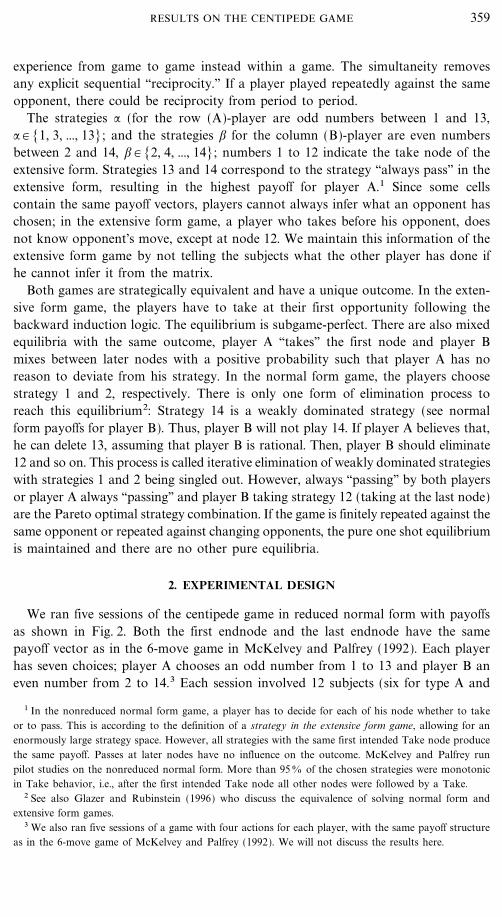
v There is no clear trend at the sessional level. Also in M�P (1992) convergenceto equilibrium is questionable (see Fig. 3 which shows the average take node in


5 McKelvey and Palfrey (1992) explain this low estimation of altruists according to their theoreticalmodel; the reason is that part of passing at the last move is attributed to errors in action and not toaltruism.

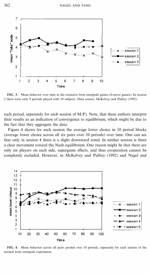
FIG. 3. Mean behavior over time in the extensive form centipede games (6-move games). In session2 there were only 9 periods played with 18 subjects. Data source: McKelvey and Palfrey (1992).

each period, separately for each session of M�P). Note, that these authors interprettheir results as an indication of convergence to equilibrium, which might be due tothe fact that they aggregate the data.

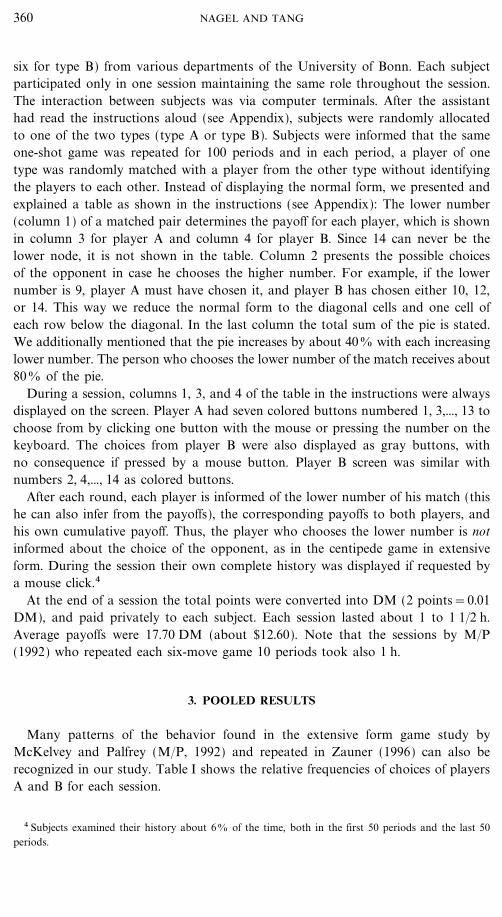
Figure 4 shows for each session the average lower choice in 10 period blocks(average lower choice across all six pairs over 10 periods) over time. One can seethat only in session 4 there is a slight downward trend. In neither session is therea clear movement toward the Nash equilibrium. One reason might be that there areonly six players on each side, supergame effects, and thus cooperation cannot becompletely excluded. However, in McKelvey and Palfrey (1992) and Nagel and

FIG. 4. Mean behavior across all pairs pooled over 10 periods, separately for each session of thenormal form centipede experiment.

362 NAGEL AND TANG

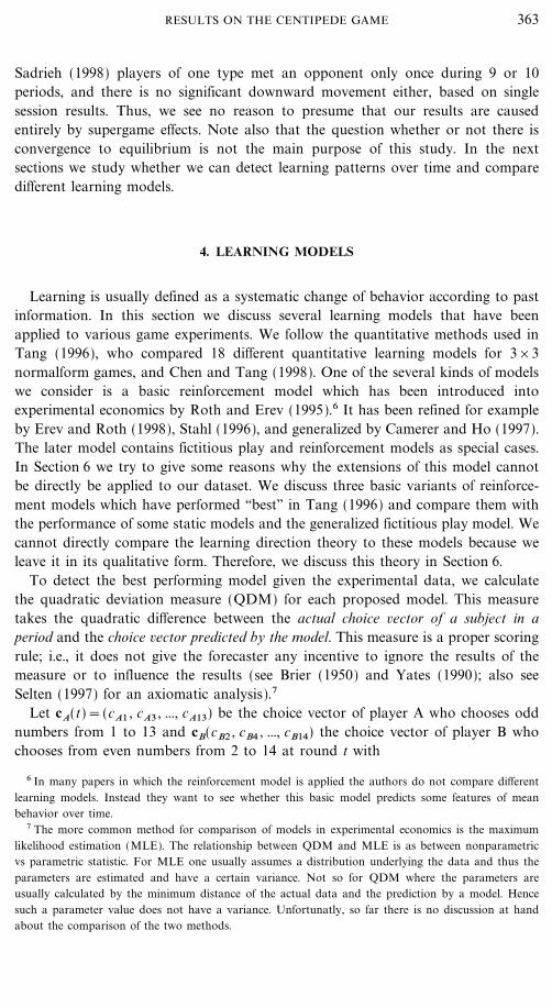
Sadrieh (1998) players of one type met an opponent only once during 9 or 10periods, and there is no significant downward movement either, based on singlesession results. Thus, we see no reason to presume that our results are causedentirely by supergame effects. Note also that the question whether or not there isconvergence to equilibrium is not the main purpose of this study. In the nextsections we study whether we can detect learning patterns over time and comparedifferent learning models.

4. LEARNING MODELS

Learning is usually defined as a systematic change of behavior according to pastinformation. In this section we discuss several learning models that have beenapplied to various game experiments. We follow the quantitative methods used inTang (1996), who compared 18 different quantitative learning models for 3_3normalform games, and Chen and Tang (1998). One of the several kinds of modelswe consider is a basic reinforcement model which has been introduced intoexperimental economics by Roth and Erev (1995).6 It has been refined for exampleby Erev and Roth (1998), Stahl (1996), and generalized by Camerer and Ho (1997).The later model contains fictitious play and reinforcement models as special cases.In Section 6 we try to give some reasons why the extensions of this model cannotbe directly be applied to our dataset. We discuss three basic variants of reinforce-ment models which have performed ``best'' in Tang (1996) and compare them withthe performance of some static models and the generalized fictitious play model. Wecannot directly compare the learning direction theory to these models because weleave it in its qualitative form. Therefore, we discuss this theory in Section 6.

To detect the best performing model given the experimental data, we calculatethe quadratic deviation measure (QDM) for each proposed model. This measuretakes the quadratic difference between the actual choice vector of a subject in aperiod and the choice vector predicted by the model. This measure is a proper scoringrule; i.e., it does not give the forecaster any incentive to ignore the results of themeasure or to influence the results (see Brier (1950) and Yates (1990); also seeSelten (1997) for an axiomatic analysis).7

Let cA(t)=(cA1 , cA3 , ..., cA13) be the choice vector of player A who chooses oddnumbers from 1 to 13 and cB(cB2 , cB4 , ..., cB14) the choice vector of player B whochooses from even numbers from 2 to 14 at round t with


6 In many papers in which the reinforcement model is applied the authors do not compare differentlearning models. Instead they want to see whether this basic model predicts some features of meanbehavior over time.

7 The more common method for comparison of models in experimental economics is the maximumlikelihood estimation (MLE). The relationship between QDM and MLE is as between nonparametricvs parametric statistic. For MLE one usually assumes a distribution underlying the data and thus theparameters are estimated and have a certain variance. Not so for QDM where the parameters areusually calculated by the minimum distance of the actual data and the prediction by a model. Hencesuch a parameter value does not have a variance. Unfortunatly, so far there is no discussion at handabout the comparison of the two methods.

cA:(t)={1,0,

if strategy : is chosen in round totherwise

;

cB;(t)={1,0,

if strategy ; is chosen in round totherwise.

Let pA(t)=( pA1 , pA3 , ..., pA13), similarly for B, denote the predicted choiceprobability vector of a particular model for player A at round t. Then the quadraticdeviation for subject A in round t is

QDMA(t)= :13

:=1

[cA:(t)&pA:(t)]2, \A # [1, 2, ..., 6], : # [1, 3, ..., 13], (1)

similarly for B # [7, 8, ..., 12], ; # [2, 4, ..., 14]. QDM(t) of a player is between 0and 2, since the choice of a player can coincide completely with the strategy pre-dicted by a model or at worst if the model predicts that a strategy has to be chosenwith probability 1 and the actual choice of a player does not coincide with it, thedeviation reaches the maximum 2. The average quadratic deviation measure perplayer and period for an entire session is

QDM=QDMA+QDMB=_:A

:100

t=1

QDMA(t)+:B

:100

t=1

QDMB(t)&<12*100. (2)

Clearly, the smaller the QDM score of a model, the better is its prediction.

4.1. Four Static Benchmark Models

The following four static models are strictly speaking not learning models, butmay serve as benchmark models to judge the relative performance of the dynamiclearning models. The static models are the equilibrium model, a quantal responsemodel, the uniform random model, and the individual-observed frequency model.

To analyze behavior in economic experiments, we usually start with the questionhow well the game theoretic solution describes actual behavior. Here we use thestage game subgame-perfect equilibrium, given that the players repeatedly play thesame game against changing opponents in finite times. To calculate the equilibriumthe entire structure of the game has to be considered.

The calculation of the QDM for the subgame-perfect equilibrium model persession and period is straightforward:

pA:(t)={1,0,

if :=1otherwise,

pB;(t)={1,0,

if ;=2otherwise;

therefore, QDM=(200&100*( f1+f2))�100, where f1 and f2 are the relativefrequencies of equilibrium strategies 1 and 2 within a session. Note that the valueof QDM(t) for a player is either 0 or 2.

Another equilibrium model is the quantal response model (McKelvey and Palfrey(M�P, 1995a)). It assumes that players do not play the equilibrium strategies of the

364 NAGEL AND TANG

original game, but make mistakes which can be interpreted as calculation errors ofexpected payoffs. Given the error rate which is common knowledge, an equilibriumis calculated. For any given *�0, the logit quantal response function is used, whichis also known in the study of individual choice behavior (Luce, 1959):

pA:(t)=e*?A:(t)

�13}=1 e*?A}(t) \A, :, and similarly for B, (3)

where * is a parameter inversely related to the error rate. For *=0 the uniformrandom distribution results and for * � �, the equilibrium of the original game isapproached. ?A: is the expected payoff for strategy : given the probability distribu-tion of strategies ;. M�P (1995b) examine the dynamics of behavior with thequantal response model by calculating *-values for period blocks 1�10, 11�20, etc.,and check the evolution of the values. We also did this and did not find that the* parameters increase over time.

The next useful benchmark model is the uniform random model, which assumesthat a player chooses each of his seven strategies with the same probability in everyround. Any selected or preferred model should certainly perform better than thismodel since it does not rely on the structure of the underlying game or situation.The vector of predicted choice probability is pA(t)=( 1

7 , 17 , 1

7 , 17 , 1

7 , 17 , 1

7) \A \t andsimilarly for B. Hence, the quadratic deviation measure for a session is

QDM={:A

:100

t=1

:13

:=1

[cA:(t)& 17]2+:

B

:100

t=1

:14

;=2

[cB;(t)& 17]2=<12*100

=[(1& 17)2+6(0& 1

7)2]=0.86. (4)

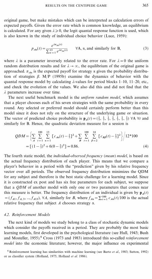
The fourth static model, the individual-observed frequency (mean) model, is based onthe actual frequency distribution of each player. This means that we compare aplayer's behavior in a period with the ``prediction'' given by his relative frequencyvector over all periods. The observed frequency distribution minimizes the QDMfor any subject and therefore is the best static challenge for a learning model. Sinceit is constructed ex post and has six free parameters for each subject, we supposethat a QDM of another model with only one or two parameters that comes nearthis measure is better. The frequency distribution of an individual is given by pA(t)=( fA1 , fA, 3 , ..., fA13), \A, similarly for B, where fA:=�100

t=1 cA:(t)�100 is the actualrelative frequency that subject A chooses strategy :.

4.2. Reinforcement Models

The next kind of models we study belong to a class of stochastic dynamic modelswhich consider the payoffs received in a period. They are probably the most basiclearning models, first developed in the psychological literature (see Hull, 1943; Bushand Mosteller, 1955).8 Cross (1973 and 1983) introduced this so-called reinforcementmodel into the economic literature; however, the major influence on experimental


8 Reinforcement learning has similarities with machine learning (see Barto et al., 1983; Sutton, 1992)or as classifier system (Holland, 1975; Holland et al. 1986).

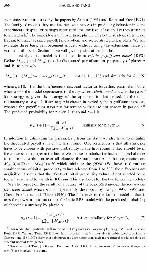
economics was introduced by the papers by Arthur (1991) and Roth and Erev (1995).The family of models they use has met with success in predicting behavior in someexperiments, despite (or perhaps because of) the low level of rationality they attributeto individuals.9 The basic idea is that over time, players play better strategies (strategiesleading to higher realized payoffs) more often, and worse strategies less often. We willevaluate three basic reinforcement models without using the extensions made byvarious authors. In Section 7 we will give a justification for this.

The first dynamic model is the linear form relative-payoff-sum model (RPS).Define MA:(t) and MB;(t) as the discounted payoff sum or propensity of player Aand B, respectively,

MA:(t)=qMA:(t&1)+cA:(t) ?A:(t), : # [1, 3, ..., 13] and similarly for B, (5)

where q # [0, 1] is the time�memory discount factor or forgetting parameter. Note,when q=0, the model degenerates to the repeat last choice model. ?A: is the payofffor strategy :, given the strategy of the opponent in that period. In the mostrudimentary case q=1, if strategy : is chosen in period t, the payoff sum increases,whereas the payoff sum stays put for strategies that are not chosen in period t.10

The predicted probability for player A at round t+1 is

pA:(t+1)=MA:(t)

�13k=1 MAk(t)

; similarly for player B. (6)

In addition to estimating the parameter q from the data, we also have to initializethe discounted payoff sum of the first round. One restriction is that all strategieshave to be chosen with positive probability in the first round if they should be inthe choice-set of a player in the future. We choose to initialize the first round probabilitiesto uniform distribution over all choices; the initial values of the propensities areMA:(0)=50 and MB;(0)=50 which minimize the QDM. (We have tried variouscombinations of initial propensity values selected from 1 to 500; the differences arenegligible. It seems that the effects of initial propensity values, if not selected to betoo extreme, tend to vanish in 100 runs. This also holds for the two following models).

We also report on the results of a variant of the basic RPS model, the power-rein-forcement model which was independently developed by Tang (1995, 1996) andChen, Friedman, and Thisse (1996). The difference to the former model is that ituses the power transformation of the basic RPS model with the predicted probabilityof choosing a strategy by player A,

pA:(t+1)=[MA:(t)]r

�13k=1 [MAk(t)]r \A, :; similarly for player B, (7)

366 NAGEL AND TANG

9 This model does particular well in mixed motive games (see, for example, Tang, 1996; and Erev andRoth, 1998). Yan and Tang (1998) show that it is better than fictitious play in public good experiments.Camerer and Ho (1997) show that reinforcement does worse than their more general model for data ondifferent normal form games.

10 See Chen and Tang (1998) and Erev and Roth (1998) for adjustment of the model if negativepayoffs are involved in a game.

where r is a nonnegative constant. When r=1, the probabilities are as in the RPSmodel. When r=0, the model degenerates to the uniform random model. Whenr>1, the relative weight of the discounted payoff sum is scaled up and when r<1it is scaled down.

The third reinforcement model we consider is the exponentialized-RPS modelwith the predicted probability

pA:(t+1)=e*MA: (t)

�13k=1 e*MAk (t) \A, :, (8)

where *�0 can be interpreted in a similar way as the power parameter r; when*=0, the uniform random model results.

Chen and Tang (1998) mention that an advantage of this functional form is thatnegative payoffs can be treated the same as positive payoffs. In our case (with non-negative payoffs) the model performs worse than the other two reinforcementmodels. This model has also been applied by Camerer and Ho (1997), Mookherjeeand Sopher (1996), and Weisbuch, Kirman, and Herreiner (1996). It can be inter-preted as a dynamic version of the quantal response model of McKelvey andPalfrey (1995a). However, it is not an equilibrium model, since the probabilitypA:(t) does not depend on the probability distribution of the opponent and no fixedpoint is calculated.

For the RPS model, the optimal discount factor q minimizing QDM was searchedat the grid size 0.05 which is fine enough; the power parameter r for the power-RPSmodel and * were searched at a grid size of 0.001 for the static quantal responsemodel and the exp.-RPS.

4.3. Generalized Fictitious Play

Fictitious play (Brown, 1951; Robinson, 1951) is a dynamic learning model oralgorithm that predicts convergence in the centipede game towards the equilibriumwithin some finite number of rounds. The reason is straightforward; in each perioda best response to the frequency distribution of the entire past is calculated. There-fore the highest choice can never be best response; 14 will not be selected, exceptmaybe in the initial rounds where each choice has a positive probability. Hence,strategy 14 will sooner or later die out. Then 13 will not be best response anymoreand so on. Slowly, but surely the choices will become lower and lower over time.We already know that the data does not show this characteristic. However, sinceit is a learning model with a long tradition in economic theory we do not want toignore it. Another reason for its application is that it contains the Cournot modelas a special case. This is also an important benchmark learning model which statesthat in each period a player gives best response to the opponent's choice of theprevious period.

According to Brown (1951) and Robinson (1951), in each period, a player makesa best response to the frequency distribution of the opponent(s) he observed in theentire past. Due to the random matching scheme we used, we will not follow thisapproach but instead calculate player's best response to the frequency distribution


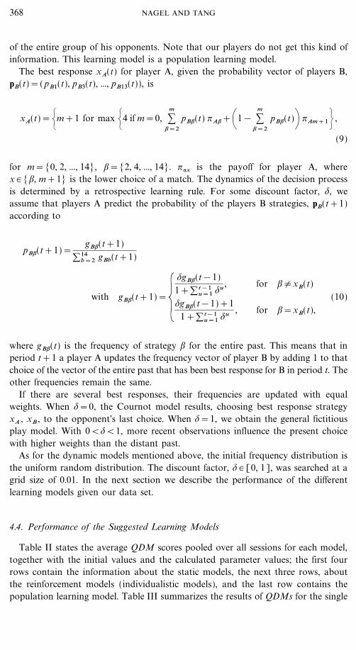
of the entire group of his opponents. Note that our players do not get this kind ofinformation. This learning model is a population learning model.

The best response xA(t) for player A, given the probability vector of players B,pB(t)=( pB1(t), pB3(t), ..., pB13(t)), is

xA(t)={m+1 for max {4 if m=0, :m

;=2

pB;(t) ?A;+\1& :m

;=2

pB;(t)+ ?Am+1= ,

(9)

for m=[0, 2, ..., 14], ;=[2, 4, ..., 14]. ?:x is the payoff for player A, wherex # [;, m+1] is the lower choice of a match. The dynamics of the decision processis determined by a retrospective learning rule. For some discount factor, $, weassume that players A predict the probability of the players B strategies, pB(t+1)according to

pB;(t+1)=gB;(t+1)

�14b=2 gBb(t+1)

with gB;(t+1)={$gB;(t&1)1+� t&1

u=1 $u ,

$gB;(t&1)+11+� t&1

u=1 $u ,

for ;{xB(t)

for ;=xB(t),(10)

where gB;(t) is the frequency of strategy ; for the entire past. This means that inperiod t+1 a player A updates the frequency vector of player B by adding 1 to thatchoice of the vector of the entire past that has been best response for B in period t. Theother frequencies remain the same.

If there are several best responses, their frequencies are updated with equalweights. When $=0, the Cournot model results, choosing best response strategyxA , xB , to the opponent's last choice. When $=1, we obtain the general fictitiousplay model. With 0<$<1, more recent observations influence the present choicewith higher weights than the distant past.

As for the dynamic models mentioned above, the initial frequency distribution isthe uniform random distribution. The discount factor, $ # [0, 1], was searched at agrid size of 0.01. In the next section we describe the performance of the differentlearning models given our data set.

4.4. Performance of the Suggested Learning Models

Table II states the average QDM scores pooled over all sessions for each model,together with the initial values and the calculated parameter values; the first fourrows contain the information about the static models, the next three rows, aboutthe reinforcement models (individualistic models), and the last row contains thepopulation learning model. Table III summarizes the results of QDMs for the single

368 NAGEL AND TANG

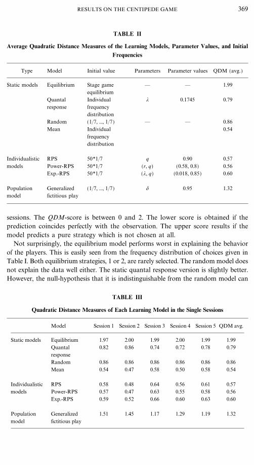
TABLE II

Average Quadratic Distance Measures of the Learning Models, Parameter Values, and InitialFrequencies

Type Model Initial value Parameters Parameter values QDM (avg.)

Static models Equilibrium Stage game �� 1.99equilibrium

Quantal Individual * 0.1745 0.79response frequency

distributionRandom (1�7, ..., 1�7) �� 0.86Mean Individual 0.54

frequencydistribution

Individualistic RPS 50*1�7 q 0.90 0.57models Power-RPS 50*1�7 (r, q) (0.58, 0.8) 0.56

Exp.-RPS 50*1�7 (*, q) (0.018, 0.85) 0.60

Population Generalized (1�7, ..., 1�7) $ 0.95 1.32model fictitious play

sessions. The QDM-score is between 0 and 2. The lower score is obtained if theprediction coincides perfectly with the observation. The upper score results if themodel predicts a pure strategy which is not chosen at all.

Not surprisingly, the equilibrium model performs worst in explaining the behaviorof the players. This is easily seen from the frequency distribution of choices given inTable I. Both equilibrium strategies, 1 or 2, are rarely selected. The random model doesnot explain the data well either. The static quantal response version is slightly better.However, the null-hypothesis that it is indistinguishable from the random model can

TABLE III

Quadratic Distance Measures of Each Learning Model in the Single Sessions

Model Session 1 Session 2 Session 3 Session 4 Session 5 QDM avg.

Static models Equilibrium 1.97 2.00 1.99 2.00 1.99 1.99Quantal 0.82 0.86 0.74 0.72 0.78 0.79responseRandom 0.86 0.86 0.86 0.86 0.86 0.86Mean 0.54 0.47 0.58 0.50 0.58 0.54

Individualistic RPS 0.58 0.48 0.64 0.56 0.61 0.57models Power-RPS 0.57 0.47 0.63 0.55 0.58 0.56

Exp.-RPS 0.59 0.52 0.66 0.60 0.63 0.60

Population Generalized 1.51 1.45 1.17 1.29 1.19 1.32model fictitious play


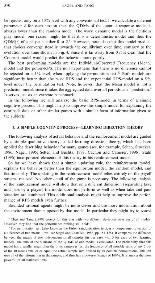
be rejected only on a 100 level with any conventional test. If we calculate a differentparameter * for each session then the QDMs of the quantal response model isalways lower than the random model. The worst dynamic model is the fictitiousplay model; one reason might be that it is a deterministic model and thus theQDM(t) of a player is either 0 or 2.11 However, note also that this model predictsthat choices converge steadily towards the equilibrium over time, contrary to theevolution over time shown in Fig. 4. Since $ is far away from 0 it is clear that theCournot model would predict the behavior more poorly.

The best performing models are the Individual-Observed Frequency (Mean)model and the power-RPS. The null hypothesis that there is no difference cannotbe rejected on a 50 level, when applying the permutation test.12 Both models aresignificantly better than the basic RPS and the exponential RPS-model on a 50

level under the permutation test. Note, however, that the Mean model is not aprediction model, since it takes the aggregated data over all periods as a ``prediction.''It serves just as an extreme benchmark.

In the following we will analyze the basic RPS-model in terms of a simplecognitive process. This might help to improve this simple model for explaining thecentipede data or other similar games with a similar form of information given tothe subjects.

5. A SIMPLE COGNITIVE PROCESS��LEARNING DIRECTION THEORY

The following analysis of actual behavior and the reinforcement model are guidedby a simple qualitative theory, called learning direction theory, which has beenapplied for describing behavior for many games (see, for example, Selten, Stoecker,1986; Nagel, 1995; Selten and Buchta, 1998; Cachon and Camerer, 1996). Stahl(1996) incorporated elements of this theory in his reinforcement model.

So far we have shown that a simple updating rule, the reinforcement model,explains the behavior better than the equilibrium model, the random model, andfictitious play. The updating in the reinforcement model relies entirely on the payoffstreams realized. No other detail of the game is necessary. The following analysisof the reinforcement model will show that on a different dimension (separating takeand pass by a player) the model does not perform as well as when take and passsituation are combined. This additional analysis might help to improve the perfor-mance of RPS models even further.

Bounded rational agents might be more clever and use more information aboutthe environment than supposed by that model. In particular they might try to search

370 NAGEL AND TANG

11 Chen and Tang (1998) correct for this bias with two different deviation measures of all models.However, they find that the performance ranking still holds.

12 For permutation test (also know as the Fisher randomization test), is a nonparametric version ofa difference of two means t-test (see Siegel and Castellan, 1988, pp. 151�155). It compares the differencebetween the means of two independent small samples (in our case with 5 for each of two learningmodel). The sum of the 5 means of the QDMs of one model is calculated. The probability that thismodel has a smaller mean than the other sample is just the frequency of all possible sums of any 5 outof the 10 means smaller or equal the actual sample sum divided by all possible permutations. This testuses all of the information in the sample, and thus has a power-efficiency of 1000. It is among the mostpowerful of all statistical tests.

for better strategies given the information in a period. This is the basic element ofa simple theory which has been called ``learning direction theory'' developed inSelten and Stoecker (1986) in experiments on repeated prisoners' dilemma super-games. This kind of reasoning can be incorporated into quantitative models as doneby Stahl (1996) for a beauty contest game and Camerer and Ho (1997) for othernormal form games. Here, we want to look at the hypotheses in isolation in orderto get a full picture of the reasoning process. Furthermore, we will explain why themodel used by Camerer and Ho (1997) reduces to the basic reinforcement modelwhen applied to our experiment.

The basic idea of the simple cognitive reasoning process is the following: Observinghis payoff in the previous period and obtaining all additional information according tothe rules of the game, a player considers in an ex-post reasoning process whether hecould have improved his payoff by a different strategy, x; i.e., was there a better strategyx<xt&1 or x>xt&1 , given the behavior of the opponent(s)? If a player intends tochange his strategy he should change it in the ``right'' direction. Since other influencesmight also guide the behavior, one might only expect a weak conformance to direc-tional learning; that is, in case of a change, more choices will go in the right directionthan in the wrong direction (see also Selten 6 Buchta, 1998). For this kind of reason-ing, the structure of the payoff function has to be known to the player. However,the player does not need to know where exactly the optimum is. It is supposed thatthe player only uses the information of the previous period.

In the centipede game each player is informed after a match whether or not hehas chosen the lower number; in extensive form language he knows whether hetook earlier (``take'') or later (``pass'') than the opponent.

After ``take'' he knows that a lower choice would have produced a lower payoff.Since he is not informed about the opponent's choice, he does not know whetherhe has already chosen the optimal number or whether higher payoffs would havebeen possible by a higher choice. He can only make a guess. Of course, after achoice 12 and 13, the players A and B, respectively, have no uncertainty, and 14can never be the lower choice. After lower choice 1 or 2 a player cannot decreasehis choice. We formulate the following hypothesis13:

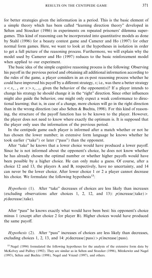
Hypothesis (1). After ``take'' decreases of choices are less likely than increases(excluding observations after choices 1, 2, 12, and 13): p(increase | take)>p(decrease | take).

After ``pass'' he knows exactly what would have been best: his opponent's choiceminus 1 (except after choice 2 for player B). Higher choices would have producedthe same payoff.

Hypothesis (2). After ``pass'' increases of choices are less likely than decreases,excluding choices 1, 2, 13, and 14: p(decrease | pass)>p(increase | pass).


13 Nagel (1994) formulated the following hypotheses for the analysis of the extensive form data byMcKelvey and Palfrey (1992). They are similar as in Selten and Stoecker (1996), Mitzkewitz and Nagel(1993), Selten and Buchta (1998), Nagel and Vriend (1997), and others.

These two formulations can also be found for the analysis of behavior in repeatedprisoner's dilemma supergames by Selten and Stoecker (1986, p. 54). Take is replacedby ``player deviates sooner than his opponent after a string of cooperation'' and passis replaced by ``player intended to deviate later than his opponent.''

We also test the hypothesis whether decreases are more likely after ``pass'' thanafter ``take'' and increases are more likely after ``take'' than after ``pass'':

Hypothesis 3. p(increase | take)>p(increase | pass).

Hypothesis 4. p(decrease | pass)>p(decrease | take).

In the next section we analyze the data with respect to the proposed hypothesesand also analyze simulations of the reinforcement model in the light of thehypotheses.

5.1. Hypotheses Testing of the Actual Data and the Reinforcement Model

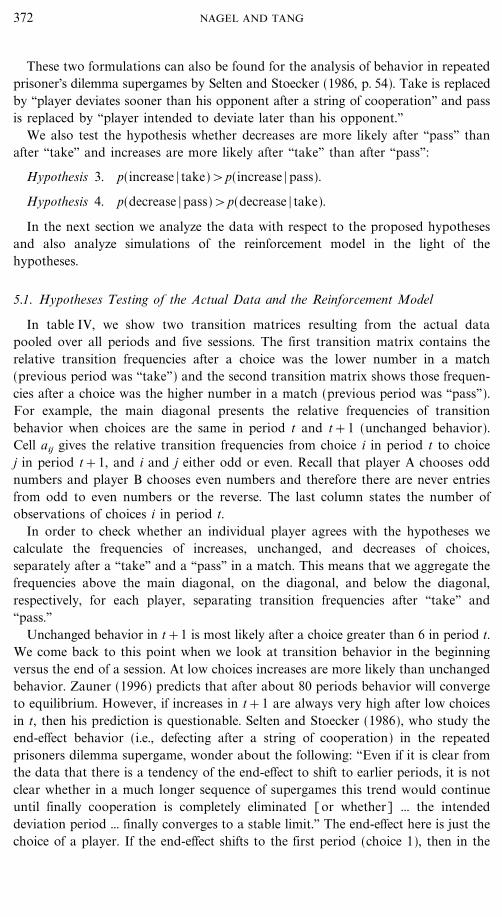
In table IV, we show two transition matrices resulting from the actual datapooled over all periods and five sessions. The first transition matrix contains therelative transition frequencies after a choice was the lower number in a match(previous period was ``take'') and the second transition matrix shows those frequen-cies after a choice was the higher number in a match (previous period was ``pass'').For example, the main diagonal presents the relative frequencies of transitionbehavior when choices are the same in period t and t+1 (unchanged behavior).Cell aij gives the relative transition frequencies from choice i in period t to choicej in period t+1, and i and j either odd or even. Recall that player A chooses oddnumbers and player B chooses even numbers and therefore there are never entriesfrom odd to even numbers or the reverse. The last column states the number ofobservations of choices i in period t.

In order to check whether an individual player agrees with the hypotheses wecalculate the frequencies of increases, unchanged, and decreases of choices,separately after a ``take'' and a ``pass'' in a match. This means that we aggregate thefrequencies above the main diagonal, on the diagonal, and below the diagonal,respectively, for each player, separating transition frequencies after ``take'' and``pass.''

Unchanged behavior in t+1 is most likely after a choice greater than 6 in period t.We come back to this point when we look at transition behavior in the beginningversus the end of a session. At low choices increases are more likely than unchangedbehavior. Zauner (1996) predicts that after about 80 periods behavior will convergeto equilibrium. However, if increases in t+1 are always very high after low choicesin t, then his prediction is questionable. Selten and Stoecker (1986), who study theend-effect behavior (i.e., defecting after a string of cooperation) in the repeatedprisoners dilemma supergame, wonder about the following: ``Even if it is clear fromthe data that there is a tendency of the end-effect to shift to earlier periods, it is notclear whether in a much longer sequence of supergames this trend would continueuntil finally cooperation is completely eliminated [or whether] ... the intendeddeviation period ... finally converges to a stable limit.'' The end-effect here is just thechoice of a player. If the end-effect shifts to the first period (choice 1), then in the

372 NAGEL AND TANG

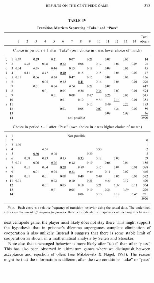
TABLE IV

Transition Matrices Separating ``Take'' and ``Pass''

Total1 2 3 4 5 6 7 8 9 10 11 12 13 14 observ

Choice in period t+1 after ``Take'' (own choice in t was lower choice of match)

c 1 0.07 0.29 0.21 0.07 0.21 0.07 0.07 14h 2 0.28 0.08 0.32 0.08 0.12 0.04 0.08 25o 3 0.04 0.09 0.44 0.13 0.18 0.09 0.02 45i 4 0.11 0.11 0.40 0.15 0.15 0.06 0.02 47c 5 0.01 0.06 0.20 0.47 0.15 0.08 0.03 156e 6 0.05 0.32 0.41 0.14 0.06 0.01 296

7 0.01 0.04 0.60 0.28 0.07 617i 8 0.01 0.05 0.56 0.36 0.02 0.01 594n 9 0.01 0.08 0.62 0.26 0.03 545

10 0.01 0.12 0.73 0.14 0.01 353t 11 0.17 0.60 0.23 173

12 0.03 0.05 0.07 0.83 0.02 5913 0.09 0.91 4614 not possible 2970

Choice in period t+1 after ``Pass'' (own choice in t was higher choice of match)

c 1 Not possibleh 2 0o 3 1.00 1i 4 0.50 0.50 2c 5 0.60 0.20 0.20 5e 6 0.08 0.23 0.15 0.33 0.18 0.03 39

7 0.01 0.06 0.25 0.48 0.10 0.06 0.04 156i 8 0.01 0.04 0.29 0.49 0.15 0.04 0.01 388n 9 0.01 0.04 0.33 0.48 0.11 0.02 446

10 0.01 0.01 0.08 0.40 0.40 0.06 0.03 572t 11 0.01 0.02 0.10 0.31 0.43 0.12 490

12 0.01 0.03 0.10 0.21 0.54 0.11 36413 0.01 0.05 0.10 0.34 0.50 27614 0.06 0.10 0.19 0.65 231

2970

Note. Each entry is a relative frequency of transition behavior using the actual data. The underlinedentries are the modal off diagonal frequencies. Italic cells indicate the frequencies of unchanged behaviour.

next centipede game, the player most likely does not stay there. This might supportthe hypothesis that in prisoner's dilemma supergames complete elimination ofcooperation is also unlikely. Instead it suggests that there is some stable limit ofcooperation as shown in a mathematical analysis by Selten and Stoecker.

Note also that unchanged behavior is more likely after ``take'' than after ``pass.''This has also been observed in ultimatum games where we distinguish betweenacceptance and rejection of offers (see Mitzkewitz 6 Nagel, 1993). The reasonmight be that the information is different after the two conditions ``take'' or ``pass''


in the centipede game or ``acceptance'' or ``rejection.'' After a ``pass'' it is clear thata decrease of the choice would have been better. In ultimatum games after``rejection'' it is clear that an increase of an offer would have increased the likeli-hood of acceptance. This is not true after a ``take'' or an ``acceptance of an offer.''In these cases one knows for sure that decreases of take nodes or increases of offersshould not be done and the going in the opposite direction only might improvepayoffs.

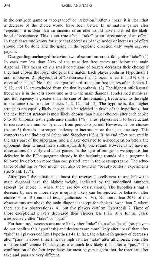
Disregarding unchanged behavior, two observations are striking after ``take'': (1)In each row less than 200 of the transition frequencies are below the maindiagonal. This means only a small percentage of players decreases their choices ifthey had chosen the lower choice of the match. Each player confirms Hypothesis 1and, moreover, 21 players out of 60 decrease their choices in less than 20 of thecases after ``take.'' Note that comparisons of transition frequencies after choices 1,2, 12, and 13 are excluded from the first hypothesis. (2) The highest off-diagonalfrequency is in the cells above and next to the main diagonal (underlined numbers)and its frequency is greater than the sum of the remaining frequencies to the rightin the same row (not for choices 1, 2, 12, and 13). The hypothesis, that higherstrategies are equally likely chosen, can be rejected in favor of the hypothesis, thatthe next highest strategy is more likely chosen than higher choices, after each choice5 to 10 (binomial test, significance smaller 10). Thus, players seem to be reluctantto increase their number by much from period to period. However, at low choices(below 5) there is a stronger tendency to increase more than just one step. Thisconnects to the findings of Selten and Stoecker (1986). If the end effect occurred inthe later part of the supergame and a player deviated to noncooperation before theopponent, then he most likely shifts upwards by one round. However, they have noobservations for early end effect games. In the light of our game we suppose thatdefection in the PD-supergame already in the beginning rounds of a supergame isfollowed by defection more than one period later in the next supergame. The reluc-tance of shifting by ``too much'' can also be found in ``beauty-contest'' experiments(see Stahl, 1996).

After ``pass'' the situation is almost the reverse: (1) cells next to and below themain diagonal have the highest weight, indicated by the underlined numbers(except for choice 6, where there are few observations). The hypothesis that adecrease by one or more steps is equally likely can be rejected for behavior afterchoices 6 to 13 (binomial test, significance <10). No more than 200 of theobservations are above the main diagonal (except for choices lower than 7, wherethere are few observations). All but five players confirm Hypothesis 2. Three ofthose exceptional players decreased their choices less than 100 for all cases,irrespectively after ``take'' or ``pass.''

Furthermore, increases are more likely after ``take'' than after ``pass'' (six playersdo not confirm this hypothesis) and decreases are more likely after ``pass'' than after``take'' (all players confirm Hypothesis 4). In fact, the relative frequency of decreasesafter ``pass'' is about three times as high as after ``take'' after all choices; even aftera ``successful'' choice 13, decreases are much less likely than after a ``pass.'' Theconfirmation of the four hypotheses for most players suggest that the reactions aftertake and pass are very different.

374 NAGEL AND TANG

Note that the patterns of learning direction theory do not necessarily imply learningto play closer to the equilibrium strategy (i.e., to decrease a choice). Furthermore, ifplayers give the best reply to a belief of the existence of altruistic players and errors,as assumed in McKelvey and Palfrey (1992) the difference of behavior betweenTake and Pass should not be that sharp. Mixed strategies cannot explain thesedifferences either. McKelvey and Palfrey (1992, p. 811) pointed out the behavior oftwo subjects who in fact behave as described by the learning direction theory.However, M�P did not notice that pattern. Instead, they called that an ``interestingnonpattern in the data, ... inconsistent with the use of a single pure strategy ... .Fairly common irregularities of this sort, ... would seem to require some degree ofrandomness to explain. While some sort of this behavior may indicate evidence ofthe use of mixed strategies, some such behavior is impossible to rationalize, even byresorting to the possibility of altruistic individuals or Bayesian updating acrossgames.''

In the following we analyze the basic reinforcement model with respect to thehypotheses of our simple cognitive process. In order to do so we run 200 simula-tions of the basic reinforcement model, with the parameter q=0.9, initial uniformfrequency distribution, and propensity weights 50 for each strategy as in Section 5.The updating after each period is similar as in the formula of the basic reinforce-ment model in Section 5. However, instead of updating the discounted payoff-sumwith the payoff resulting from the actual choice of a player in a session, the updatingfollows from the choice resulting of the draw according to the probability distributionafter each period,14

MAi(t)=qM:(t&1)+c$A:(t) ?Ai:(t), : # [1, 3, ..., 13]; similarly for B, (11)

where c$Ai:(t)=1 results from the draw of the probability distribution:

pA:(t)=MA:(t&1)

�13k=1 MAk(t&1)

\A, :; similarly for player B. (12)

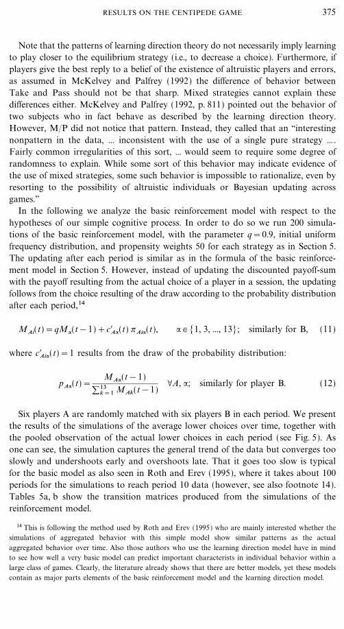
Six players A are randomly matched with six players B in each period. We presentthe results of the simulations of the average lower choices over time, together withthe pooled observation of the actual lower choices in each period (see Fig. 5). Asone can see, the simulation captures the general trend of the data but converges tooslowly and undershoots early and overshoots late. That it goes too slow is typicalfor the basic model as also seen in Roth and Erev (1995), where it takes about 100periods for the simulations to reach period 10 data (however, see also footnote 14).Tables 5a, b show the transition matrices produced from the simulations of thereinforcement model.


14 This is following the method used by Roth and Erev (1995) who are mainly interested whether thesimulations of aggregated behavior with this simple model show similar patterns as the actualaggregated behavior over time. Also those authors who use the learning direction model have in mindto see how well a very basic model can predict important characterists in individual behavior within alarge class of games. Clearly, the literature already shows that there are better models, yet these modelscontain as major parts elements of the basic reinforcement model and the learning direction model.

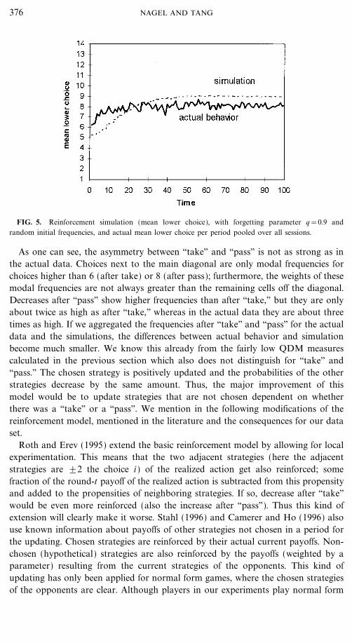
FIG. 5. Reinforcement simulation (mean lower choice), with forgetting parameter q=0.9 andrandom initial frequencies, and actual mean lower choice per period pooled over all sessions.

As one can see, the asymmetry between ``take'' and ``pass'' is not as strong as inthe actual data. Choices next to the main diagonal are only modal frequencies forchoices higher than 6 (after take) or 8 (after pass); furthermore, the weights of thesemodal frequencies are not always greater than the remaining cells off the diagonal.Decreases after ``pass'' show higher frequencies than after ``take,'' but they are onlyabout twice as high as after ``take,'' whereas in the actual data they are about threetimes as high. If we aggregated the frequencies after ``take'' and ``pass'' for the actualdata and the simulations, the differences between actual behavior and simulationbecome much smaller. We know this already from the fairly low QDM measurescalculated in the previous section which also does not distinguish for ``take'' and``pass.'' The chosen strategy is positively updated and the probabilities of the otherstrategies decrease by the same amount. Thus, the major improvement of thismodel would be to update strategies that are not chosen dependent on whetherthere was a ``take'' or a ``pass''. We mention in the following modifications of thereinforcement model, mentioned in the literature and the consequences for our dataset.

Roth and Erev (1995) extend the basic reinforcement model by allowing for localexperimentation. This means that the two adjacent strategies (here the adjacentstrategies are \2 the choice i ) of the realized action get also reinforced; somefraction of the round-t payoff of the realized action is subtracted from this propensityand added to the propensities of neighboring strategies. If so, decrease after ``take''would be even more reinforced (also the increase after ``pass''). Thus this kind ofextension will clearly make it worse. Stahl (1996) and Camerer and Ho (1996) alsouse known information about payoffs of other strategies not chosen in a period forthe updating. Chosen strategies are reinforced by their actual current payoffs. Non-chosen (hypothetical) strategies are also reinforced by the payoffs (weighted by aparameter) resulting from the current strategies of the opponents. This kind ofupdating has only been applied for normal form games, where the chosen strategiesof the opponents are clear. Although players in our experiments play normal form

376 NAGEL AND TANG

TABLE V

Transition Matrices Separating ``Take'' and ``Pass''

Total1 2 3 4 5 6 7 8 9 10 11 12 13 14 observ

Choice in period t+1 after ``Take'' (own choice in t was lower choice of match)

c 1 0.10 0.11 0.12 0.17 0.18 0.18 0.15 60h 2 0.10 0.11 0.12 0.18 0.21 0.17 0.12 64o 3 0.09 0.11 0.11 0.17 0.19 0.18 0.16 64i 4 0.07 0.12 0.13 0.19 0.22 0.16 0.11 78c 5 0.05 0.06 0.27 0.17 0.19 0.14 0.12 102e 6 0.04 0.05 0.23 0.22 0.21 0.16 0.09 162

7 0.02 0.02 0.04 0.64 0.11 0.09 0.08 341i 8 0.01 0.02 0.05 0.49 0.23 0.15 0.04 521n 9 0.01 0.01 0.02 0.04 0.81 0.06 0.05 539

10 0.01 0.01 0.03 0.13 0.61 0.17 0.04 531t 11 0.01 0.01 0.01 0.03 0.05 0.84 0.05 292

12 0.01 0.01 0.03 0.10 0.18 0.62 0.04 20513 0.02 0.03 0.03 0.04 0.06 0.07 0.76 4314 Not possible 3000

Choice in period t+1 after ``Pass'' (own choice in t was higher choice of match)

c 1 Not possibleh 2 0.10 0.14 0.15 0.15 0.20 0.14 0.12 5o 3 0.10 0.13 0.11 0.20 0.19 0.11 0.16 6i 4 0.11 0.13 0.13 0.20 0.17 0.13 0.14 14c 5 0.09 0.11 0.20 0.15 0.16 0.16 0.13 15e 6 0.08 0.10 0.19 0.21 0.18 0.13 0.12 29

7 0.05 0.06 0.08 0.53 0.11 0.09 0.09 65i 8 0.02 0.04 0.09 0.49 0.20 0.11 0.05 177n 9 0.02 0.02 0.03 0.07 0.77 0.06 0.04 320

10 0.02 0.02 0.05 0.19 0.55 0.13 0.04 481t 11 0.01 0.01 0.02 0.05 0.06 0.81 0.04 585

12 0.01 0.02 0.04 0.14 0.22 0.53 0.04 55313 0.01 0.02 0.02 0.05 0.07 0.07 0.76 56914 0.05 0.05 0.09 0.18 0.25 0.19 0.18 180

3000

Note. Each entry is a relative frequency of transition behavior using the reinforcement simulations.The underlined entries are the modal off diagonal frequencies. Italic cells indicate the frequencies ofunchanged behaviour.

games, they cannot always deduce from the payoff matrix what their opponentchose. This is the case for the player who chooses the lower choice in a match.However, one could apply Camerer and Ho's mechanism to restrict the updatingto the observed information of the players: In a match in which a player has chosenthe lower number, only those of his strategies equal to and below his current choicecan be updated since the player knows these payoffs in that case. Of course, lower(hypothetical) choices produce lower payoffs. In case a player has chosen the highernumber of his match, all strategies are updated, since he knows what the opponent


has chosen. The payoffs for (hypothetical) choices above his actual choice are thesame as for his actual choice. The highest payoff is obtained for the choice just onebelow the opponents choice. This kind of updating would mean that after ``take''decreases become more likely than increases, and after ``pass'' best response choicesbecome most strongly updated. These choices might not be next and below themain diagonal. A similar point has been made by Vriend (1997) in connection withultimatum games. A promising extension suggested by Camerer and Ho which wasinspired by discussions about our data is to reinforce unchosen strategies after``take'' by some elements of the set of forgone payoffs. This means, that after take,choices above the chosen take nodes are updated by for, e.g. the median payoff, ora combination of minimum or maximum payoff possibly gained with these higherchoices. This will generate transition probabilities similar to those reported inTable 4 after take.

Another aspect which we feel worth mentioning is the transition behavior overtime, that is, at the beginning versus at the end of the experiment. From the psycho-logical literature, it is well known that learning takes place in the beginning of a

FIG. 6. Transition behavior of actual choices pooled over 10-periods, separately for ``take'' (a) and``pass'' (b). E.g., the decrease line after ``pass'' for example means how many players in 0 chose a lowernode after observing that their choice was higher choice of match.

378 NAGEL AND TANG

new situation. In order to put this hypothesis in operation, we pool transition behavioracross 10 periods and aggregate the relative frequencies of increased, decreased, orunchanged behavior across choices, respectively, separately for ``previous periodwas take'' and for ``previous period was pass.'' In other words we aggregate the cellsabove, the cells below the main diagonal and the diagonal cells, respectively foreach block of 10-period transition matrix. Figure 6 shows the development of thetransition behavior (increased, decreased, unchanged) for each of the 10-periodblocks pooled over all sessions, separately for ``take'' and ``pass.''

In the opening periods behavior according to learning direction theory has thehighest frequency, which is the sum of relative frequencies of increases after takeand those of decreases after pass. This holds for all five sessions, separately as well.A similar feature has been observed in Duffy and Nagel (1997). In the centipedegame unchanged behavior receives increasing importance with highest frequencyafter about 50 periods in all sessions, except after ``pass'' in session 3. Thus, in thecentipede game, most learning takes place in the beginning. This is an observation

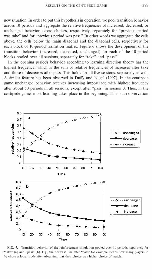
FIG. 7. Transition behavior of the reinforcement simulation pooled over 10-periods, separately for``take'' (a) and ``pass'' (b). E.g., the decrease line after ``pass'' for example means how many players in0 chose a lower node after observing that their choice was higher choice of match.


which is called the law of effect. Only after pass there is still substantial movementtowards the equilibrium (see relative frequencies of decreases after pass). If unchangedbehavior increased even more in a longer time horizon, it is questionable whetheractual behavior would ever converge towards the one-stage equilibrium, as suggestedby Zauner (1996). Clearly, the reinforcement model also predicts an increase ofunchanged behavior. However, increases after Take and decreases after Pass are toomuch reduced and the difference between right or wrong direction is less sharp,especially after Take (see Fig. 7).

6. CONCLUSION

We have analyzed behavior on the centipede game played in the reduced normalform. The main advantage of the strategic form over the extensive form is thatplayers have to reveal the intended take node, information that is interesting tostudy the adaptation of a player from period to period. We have compared differentlearning models which have been predominant in the experimental literature.

McKelvey and Palfrey (1992), Fey, McKelvey, and Palfrey (1994), and McKelveyand Palfrey (1996b) explain the behavior in centipede games by ex-ante rationalityand by using equilibrium models with errors in beliefs or actions. We show that thetwo equilibrium models, the standard Nash equilibrium and the quantal responsemodel (McKelvey 6 Palfrey (1996a) perform much worse than simple reinforcementmodels. This model is also better than fictitious play.

Another important aspect of this paper was to analyze behavior in terms of asimple ex-post reasoning process which prescribes in which direction the behaviorshould be changed from period to period. Because of the structure of the centipedegame, we were able to discuss the qualitative learning direction theory in muchgreater depth than in any of the previous papers, where this theory has beenapplied. In particular, we were able to disaggregate transition behavior from periodt to period t+1 after each possible choice in period t and also the transitionbehavior in earlier periods, in comparison to later periods. We found that mostsubjects conform on average to the qualitative learning theory. In the first periodsthis holds more often than in later periods, when unchanged behavior tends todominate. The most robust finding is that decreases after Pass occur almost threetimes as much as after Take at each node; after Take increases are more likely thandecreases and after Pass decreases are more likely than increases. This calls us toquestion the interpretation of the data by McKelvey and Palfrey (1992) that playersadjust their behavior according to a model of incomplete information about altruists.Because unchanged behavior increases over time, Zauner's predictions of convergencetowards the equilibrium is also questionable. At least we showed that they do notconverge within 100 periods as he hypothesized. The extension to a simple reinfor-cement model introduced by Roth and Erev (1995) and Camerer and Ho (1997)cannot explain the differences of transition behavior after take and pass either. Thelater so far applies only to normalform games with exact information of opponentsstrategies. A modification of their model to extensive form games or games withextensive form information as in our game should be possible.

380 NAGEL AND TANG

Since we gave the extensive form information to the subjects, we hope that ouranalysis will inspire improvements of learning models for experiments of gamesplayed in extensive form or with extensive form information as in ours. The maindifficulty of improving learning models for extensive form games is that a playermight not receive information of behavior of opponents in subgames not reachedin a period. This means that the updating of unchosen choices might have to bebased on unobservable information.

APPENDIX

Instructions

�� Each participant has to make a decision in each of 100 rounds.

�� There are two different types: six participants are of type A and six are oftype B.

�� At the beginning of the experiment you will know your type, which is thesame for the entire experiment.

�� A type A always meets a type B and a type B always meets a type A.

�� In each round, it is randomly determined which type A meets which type B.

�� A and B simultaneously choose a number out of the following numbers:

�� A chooses a number from [1, 3, 5, 7, 9, 11, 13],

�� B chooses a number from [2, 4, 6, 8, 10, 12, 14].

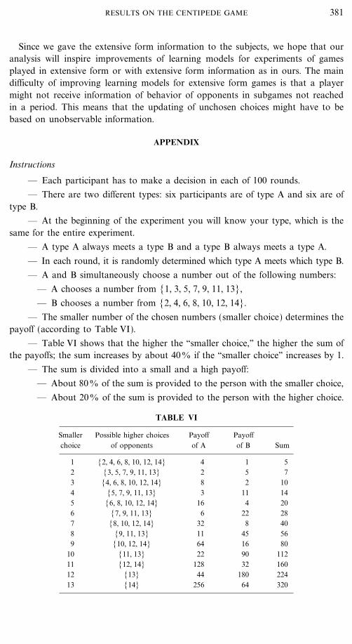
�� The smaller number of the chosen numbers (smaller choice) determines thepayoff (according to Table VI).

�� Table VI shows that the higher the ``smaller choice,'' the higher the sum ofthe payoffs; the sum increases by about 400 if the ``smaller choice'' increases by 1.

�� The sum is divided into a small and a high payoff:

�� About 800 of the sum is provided to the person with the smaller choice,

�� About 200 of the sum is provided to the person with the higher choice.

TABLE VI

Smaller Possible higher choices Payoff Payoffchoice of opponents of A of B Sum

1 [2, 4, 6, 8, 10, 12, 14] 4 1 52 [3, 5, 7, 9, 11, 13] 2 5 73 [4, 6, 8, 10, 12, 14] 8 2 104 [5, 7, 9, 11, 13] 3 11 145 [6, 8, 10, 12, 14] 16 4 206 [7, 9, 11, 13] 6 22 287 [8, 10, 12, 14] 32 8 408 [9, 11, 13] 11 45 569 [10, 12, 14] 64 16 80

10 [11, 13] 22 90 11211 [12, 14] 128 32 16012 [13] 44 180 22413 [14] 256 64 320


Information

�� At the end of each round, each participant is informed about his result ofthe round:

�� the lower choice

�� the payoffs to A and B.

�� You will not know with whom you were matched. You will know onlyabout the choice of the other, if his number was the lower choice.

Payoffs

�� The sum of the payoffs of all rounds of a participant is his total gain.

�� The exchange rate is 0.01 DM for 2 points, thus 1000 points is 5 DM.

REFERENCES

Arthur, B. (1991). Designing economic agents that act like human agents: A behavioral approach tobounded rationality. American Economic Review, Papers and Proceedings, 81, 353�409.

Aumann, B. (1992). Irrationality in Game Theory. In P. Dasgupta, D. Gale, O. Hart, 6 E. Maskin(Eds.), Economic analysis of markets and games, pp. 214�227. Cambridge, MA: MIT Press.

Binmore, K. (1988). Modeling rational players, I, II. Economics and Philosophy, 3, 179�214; 4, 9�55.

Barto, A. G., Sutton, R. S., 6 Anderson, C. W. (1983). Neuronlike adaptive elements that can solvedifficult learning control problems. IEEE Transactions on Systems, Man, and Cybernetics, 13(5),834�846.

Brier, G. W. (1950). Verification of forecasts expressed in terms of probability. Monthly Weather Review,78, 1�3.

Brown, G. (1951). Iterative solution of games by fictitious play. In T. Koopsmans (Ed.), Activity analysisof production and allocation, pp. 374�376. New York: Wiley.

Bush, R. R., 6 Mosteller, F. (1955). Stochastic models of learning. New York: Wiley.

Cason, 6 Camerer, C. (1996). The sunk cost fallacy, forward induction and behavior in coordinationgames. Quarterly Journal of Economics, 111, 165�194.

Camerer, C., 6 Ho, T. (1997). Experience-weighted attraction learning in games: A unifying approach.Caltech working paper 1003.

Chen, Y., 6 Tang, F. F. (1998). Learning and incentive compatible mechanism for public goodsprovision: An experimental study. Journal of Political Economics.

Chen, H., Friedman, J., 6 Thisse, J.-F. (1996). Boundedly rational Nash-equilibrium: A probabilisticapproach. Games and Economic Behavior.

Cressmann, R., 6 Schlag, K. H. (1996). The dynamic (in)stability of backwards induction. University ofBonn, mimeo.

Cross, J. G. (1973). A stochastic learning model of economic behavior, Quarterly Journal of Economics,87, 239�266.

Cross, J. G. (1983). A theory of adaptive economic behavior. Cambridge: Cambridge University Press.

Duffy, J., 6 Nagel, R. (1997). On the robustness of behaviour in experimental ``beauty-contest games'',Economic Journal, 107, 1684�1700.

Erev, I., 6 Roth, A. (1998), On the need for low rationality, cognitive game theory: Reinforcementlearning in experimental games with unique mixed strategy equilibria. American Economic Review.

382 NAGEL AND TANG

Fey, M., Mckelvey, R. D., 6 Palfrey, T. R. (1994). Experiments on the constant-sum centipede game.Caltech working paper.

Glazer, J., 6 Rubinstein, A. (1996). An extensive game as a guide for solving a normal game. Games andEconomic Behavior, 70, 32�42.

Gueth, W., Ockenfels, P., 6 Wendel, M. (1993). Efficiency by trust in fairness? Multiperiod ultimatumbargaining experiments with an increasing cake. International Journal of Game Theory, 22, 51�73.

Van Huyck, J. B., Battalio, R. C., 6 Beil, R. O. (1990). Tacit coordination games, strategic uncertainty,and coordination failure. American Economic Review, 80, 234�248.

Holland, J. H. (1975). Adaptation in natural and artificial systems. Ann Arbor: University of MichiganPress.

Holland, J. H., Holyoak, K. J., Nisbett, R. E., 6 Thagard, P. R. (1986). Induction: Processes of inference,learning, and discovery, Cambridge, MA: MIT Press.

Hull, C. L. (1943). Principles of behavior. New York: Appleton�Century�Crofts.

Kreps, D., Milgrom, P., Roberts, T., 6 Wilson, R. (1982). Rational cooperation in the finitely repeatedprisoners' dilemma. Journal of Economic Theory, 27, 245�252.

Luce, R. D. (1959). Individual choice behavior. New York: Wiley.

Mckelvey, R. D., 6 Palfrey, T. R. (1992). An experimental study of the centipede game. Econometrica,60, 803�836.

Mckelvey, R. D., 6 Palfrey, T. R. (1995a). Quantal response equilibria for normal form games. Gamesand Economic Behavior, 10, 6�38.

Mckelvey, R. D., 6 Palfrey, T. R. (1995b). Quantal response equilibria for extensive form games.Caltech, mimeo.

Mookherjee, D., 6 Sopher, B. (1996). Learning and decision costs in experimental constant sum games.Mimeo.

Mitzkewitz, M., 6 Nagel, R. (1993). Experimental results on ultimatum games with incomplete information.International Journal of Games Theory, 22, 171�198.

Nagel, R. (1994). Reasoning and learning in guessing games and ultimatum games with incompleteinformation: An experimental investigation. University Bonn disseration.

Nagel, R. (1995). Unraveling in guessing games: An experimental study. American Economic Review85(5), 1313�1326.

Nagel, R., 6 Vriend, N. (1997). A study of adaptive behavior in oligopolistic market games, WorkingPaper 230, Universitat Pompeu Fabra.

Nagel, R., 6 Sadrieh (1998). A comparison of behavior in extensive form 6 normal form centipedegames. In preparation.

Neugebauer, T. (1994). Experimente mit dem ``Centipede''-spiel in normalform, Diplomarbeit, Universityof Bonn.

Ponti, G. (1996). Cycles of learning in the centipede game. University College London. mimeo.

Robinson, J. (1951). An iterative method of solving a game. Annals of Mathematics, 54, 296�301.

Rosenthal, R. (1981). Games of perfect information, predatory pricing, and the chain store paradox.Journal of Economic Theory, 25, 92�100.

Roth, A. E., 6 Erev, I. (1995). Learning in extensive-form games: Experimental data and simple dynamicmodels in the intermediate term. Games and Economic Behavior, 8, 164�212.

Selten, R. (1997). Axiomatic characterization of the quadratic scoring rule, Discussion Paper No. B-390,University of Bonn.

Selten, R., 6 Stoecker, R. (1986). End behavior in sequences of finite prisoner's dilemma supergames,a learning theory approach. Journal of Economic Behavior, 47�70.

Selten, R., 6 Buchta, J. (1998). Experimental sealed bid first price auction with directly observed bidfunctions. In D. Budescu, I. Erev, 6 R. Zwick (Eds.), Games and human behavior, essays in honor ofAmnon Rapoport. Hillsdale, NJ: Erlbaum.


Siegel, S., 6 Castellan, N. J. (1988). Nonparametric statistics for the behavioral sciences. New York:McGraw�Hill.

Stahl, D. O. (1996). Bounded rational rule-learning in a guessing game. Games and Economic Behavior,16(2), 303�330.

Sutton, R. S. (1992). Introduction: The challenge of reinforcement learning. Machine Learning, 8, 3�4,225�227.

Tang, F. F. (1996). Anticipatory learning in two-person games: an experimental study. Part II. Learning.Sfb-Discussion Paper B-363, University of Bonn.

Vriend, N. (1997). Will reasoning improve learning? Economics Letters, 1997, 55(1), pp. 9�18.

Weisbuch, G., Kirman, A., 6 Herreiner, D. (1996). Market organization, mimeo.

Yates, F. J. (1990). Judgment and decision making. Englewood Cliffs, NJ: Prentice�Hall.

Zauner, K. G. (1996). A payoff uncertainty explanation of results in experimental centipede games. Workingpaper 96-030, University of New South Wales.

Received March 16, 1998

384 NAGEL AND TANG

experimental results on the centipede game in normal form: an

Documents