Noise Figure Measurement Accuracy –The Y-Factor Method

Application Note 57-2

2

Table of contents1 Introduction.....................................................................................................................................................4

2 Noise figure measurement ...........................................................................................................................5

2.1 Fundamentals ..............................................................................................................................................5

2.1.1 What is noise figure? ..........................................................................................................................5

2.1.2 What is noise temperature? ..............................................................................................................6

2.1.2.1 Thermal noise power .............................................................................................................6

2.1.2.2 Noise temperature..................................................................................................................6

2.1.3 Noise figure in multi-stage systems .................................................................................................8

2.2 Y-factor measurement.................................................................................................................................8

2.2.1 Excess Noise Ratio (ENR)..................................................................................................................9

2.2.2 Y-factor .................................................................................................................................................9

2.2.3 Calibration .........................................................................................................................................10

2.2.4 Measurement with DUT...................................................................................................................10

2.2.5 Calculation of gain............................................................................................................................11

2.2.6 Second stage correction...................................................................................................................11

2.2.7 Summary ............................................................................................................................................11

3 Avoidable measurement errors .................................................................................................................12

3.1 Prevent interfering signals.......................................................................................................................12

3.2 Select the appropriate noise source.......................................................................................................13

3.2.1 Frequency coverage..........................................................................................................................13

3.2.2 Identity check....................................................................................................................................14

3.2.3 Use low ENR whenever possible ....................................................................................................14

3.2.4 When NOT to use low ENR..............................................................................................................14

3.2.5 Avoid adapters ..................................................................................................................................15

3.3 Use a preamplifier where necessary......................................................................................................15

3.4 Minimize mismatch uncertainties ..........................................................................................................15

3.4.1 Use an isolator or attenuator pad..................................................................................................16

3.4.2 Minimize change in ρ of noise source ...........................................................................................16

3.4.3 Measures of mismatch .....................................................................................................................16

3.4.3.1 VSWR: Voltage Standing Wave Ratio.................................................................................16

3.4.3.2 Reflection coefficient...........................................................................................................17

3.4.3.3 Return loss ............................................................................................................................17

3.4.3.4 S parameters.........................................................................................................................17

3.4.4 Mismatch-related errors ..................................................................................................................17

3.5 Use averaging to avoid display jitter ......................................................................................................18

3.6 Avoid non-linearity or unstable performance ......................................................................................20

3.6.1 Non-linearity......................................................................................................................................20

3

3.6.2 Unstable performance......................................................................................................................20

3.7 Choose the appropriate measurement bandwidth ..............................................................................21

3.8 Account for frequency conversion..........................................................................................................22

3.8.1 Double sideband or single sideband measurement?...................................................................22

3.8.2 Estimating SSB noise figure from a DSB measurement.............................................................23

3.8.3 Local oscillator noise and leakage .................................................................................................24

3.8.4 What to check....................................................................................................................................25

3.9 Account for any other insertion losses..................................................................................................25

3.10 Correct for physical temperatures .....................................................................................................26

3.10.1 Noise source.......................................................................................................................................26

3.10.2 Noise generated in resistive losses ................................................................................................27

4 Loss and temperature corrections ...........................................................................................................27

4.1 Losses before the DUT..............................................................................................................................28

4.2 Losses after the DUT ................................................................................................................................28

4.3 Combined corrections ..............................................................................................................................28

4.4 Temperature of noise source ...................................................................................................................28

5 Calculating unavoidable uncertainties ....................................................................................................29

5.1 Example system.........................................................................................................................................29

5.2 Example of uncertainty calculation .......................................................................................................30

5.3 Step by step................................................................................................................................................31

5.4 Software tools ............................................................................................................................................33

5.4.1 RSS calculations................................................................................................................................34

5.4.2 TAG4 calculations .............................................................................................................................34

5.5 Effects of loss corrections on uncertainty ............................................................................................34

6 Practical implications..................................................................................................................................36

6.1 Sources of uncertainty .............................................................................................................................36

6.2 Instrument noise figure and instrument errors...................................................................................37

6.3 Uncertainty versus DUT noise figure and gain ....................................................................................38

6.4 A possible solution – re-define the ‘DUT’ .............................................................................................38

6.5 How to use a preamplifier .......................................................................................................................39

6.5.1 When to use a preamplifier.............................................................................................................39

6.5.2 When not to use a preamplifier......................................................................................................39

6.5.3 How to calibrate the system............................................................................................................39

6.6 Solutions – reduce ENR uncertainty......................................................................................................40

7 Checklist for improving measurement accuracy ...................................................................................41

Appendix A: Symbols and abbreviations.........................................................................................................42

Appendix B: Derivation of the RSS uncertainty equation ..........................................................................43

Appendix C: Connector care ..............................................................................................................................44

4

1 IntroductionWhy is noise figure important?Noise figure is a key performance parameter inmany RF systems. A low noise figure providesimproved signal/noise ratio for analog receivers,and reduces bit error rate in digital receivers. As a parameter in a communications link budget, a lower receiver noise figure allows smaller antennas or lower transmitter power for the same system performance.

In a development laboratory, noise figure measurements are essential to verify new designs and support existing equipment.

In a production environment, low-noise receiverscan now be manufactured with minimal need for adjustment. Even so, it is still necessary tomeasure noise figure to demonstrate that the product meets specifications.

Why is accuracy important?Accurate noise figure measurements have significant financial benefits. For many products, aguaranteed low noise figure commands a premiumprice. This income can only be realized, however,if every unit manufactured can be shown to meetits specification.

Every measurement has limits of accuracy. If a premium product has a maximum specified noisefigure of 2.0dB, and the measurement accuracy is±0.5dB, then only units that measure 1.5dB orlower are marketable. On the other hand, if theaccuracy is improved to ±0.2dB, all products measuring up to 1.8dB could be sold at the premium price.

Customers need accurate noise figure measure-ments to confirm they are getting the performancethey have paid for. Using the same example, anaccuracy of ±0.5dB for measuring a product that amanufacturer has specified as ‘2.0dB maximum’would require the acceptance of units measuringas high as 2.5dB. An improved accuracy of ±0.2dBsets the acceptance limit at 2.2dB.

Speed of measurement is also an issue. High-valueproducts favor accuracy; high-volume productsfavor speed. Due to the random nature of noiseand the statistical aspects of measuring it, there is always a trade-off between speed and accuracy.

To optimize the trade-off, it is necessary to eliminate all avoidable errors and to quantify the uncertainties that remain.

This Application Note demonstrates how toimprove noise figure measurement accuracy by following a three-stage process:

1. Avoid mistakes when making measurements

2. Minimize uncertainties wherever that is possible

3. Quantify the uncertainties that remain.

This Application Note covers the following topics:

• Fundamentals of noise figure measurement using the Y-factor method. (Chapter 2)

• Noise figure mistakes to avoid (Chapter 3)

• Measurement corrections to improve accuracy (Chapter 4)

• Calculation of the remaining uncertainties – including software tools (Chapter 5)

• Other techniques that can reduce uncertainties (Chapter 6)

• Checklist for improving accuracy (Chapter 7).

Agilent Technologies Application Note 57-1,‘Fundamentals of RF and Microwave Noise FigureMeasurements’ covers basic concepts behind making noise figure measurements. These basicconcepts covered in Application Note 57-1 areexpanded on in Chapter 2 of this Application Note.

This Application Note is specific to instrumentsthat use the Y-factor method for noise figure meas-urement. Various features of Agilent Technologiesproducts are mentioned as illustrative examples ofthe newest generation of noise figure analyzers and noise sources. Other products, however, maybe used with the techniques discussed in this document.

5

2 Noise figure measurementThis chapter outlines the fundamental features of the Y-factor measurement technique for noisefigure. Many instruments use the Y-factor technique, including:

• Agilent Technologies NFA Series noise figure analyzers

• Agilent Technologies PSA Series spectrum analyzer with noise figure measurement personality

• Agilent Technologies ESA-E Series spectrum analyzer with noise figure measurement personality

• Spectrum analyzers with ‘noise figure measurement personality’ software.

The equations developed in this chapter follow the internal calculation route of the AgilentTechnologies NFA series noise figure analyzers.The calculation routes of other noise figure instruments that use the Y-factor method areinevitably similar.

This chapter departs from previous explanationsof noise figure calculations by making extensiveuse of the noise temperature concept. Althoughnoise temperature may be less familiar, it gives atruer picture of how the instruments actually work– and most important, how they apply correctionsto improve accuracy.

2.1 Fundamentals2.1.1 What is noise figure?As explained in Agilent Technologies ApplicationNote 57-1, ‘Fundamentals of RF and MicrowaveNoise Figure Measurements’, the fundamental definition of noise figure F is the ratio of:

(signal/noise power ratio at the input of the device under test)(signal/noise power ratio at the output of the device under test)

Or alternatively:

F = (Sin/Nin)/(Sout/Nout) (2-1)

Noise figure represents the degradation insignal/noise ratio as the signal passes through adevice. Since all devices add a finite amount ofnoise to the signal, F is always greater than 1.Although the quantity F in equation (2-1) has historically been called ‘noise figure’, that name is now more commonly reserved for the quantityNF, expressed in dB:

NF = 10 log10F dB (2-2)

Agilent Technologies literature follows the contemporary convention that refers to the ratio F as ‘noise factor’, and uses ‘noise figure’ to referonly to the decibel quantity NF.

From the fundamental definition in equation (2-1)a number of useful secondary equations for noisefigure can be derived. Equally fundamental is theconcept of noise temperature. Many of the internalcomputations of an automatic noise figure analyzerare carried out in terms of noise temperature, so it is important to understand this concept well(see Section 2.1.2: What is noise temperature?).

Expressed in terms of noise temperature, the noisefactor F is given by:

F = 1 + Te/T0 (2-3)

Te is the effective (or equivalent) input noise temperature of the device. Equation (2-3) alsointroduces a reference temperature T0 which isdefined as 290K (16.8°C, 62.2°F). See ApplicationNote 57-1 for details of this derivation. The tablebelow shows a few comparisons between NF, F and Te.

Noise Noise Noise figure factor temperature

NF F Te

0dB 1 0K(absolute zero)

1dB 1.26 75.1K 3dB 2.00 290K

10dB 10 2,610K 20dB 100 28,710K

6

2.1.2 What is noise temperature?Anyone concerned with noise measurementsshould thoroughly understand the concepts ofnoise figure, noise temperature and their relationship.

Any electrical conductor contains electrons whichare somewhat free to move around – more so ingood conductors, less so in near-insulators. At normal temperatures, electrons are in randommotion, although on average there is no net motionunless an electromotive force is applied. This random motion of electrons constitutes a fluctuating alternating current that can be detected as random noise.

At any temperature above absolute zero (where allrandom motion stops) the thermal noise powergenerated in a conductor is proportional to itsphysical temperature on the absolute scale (measured in kelvin, K). Thermal noise is spreadevenly over the electromagnetic spectrum (tobeyond 5,000 GHz), and therefore the noise power detected by a receiver is proportional to the bandwidth in which the noise is measured.

2.1.2.1 Thermal noise powerThe basic relationship between thermal noisepower PN, temperature T and bandwidth is:

PN = kTB (2-4)where PN is the noise power (watts)

k is Boltzmann’s constant, 1.38 x 10-23 J/K (joules per kelvin)B is the bandwidth (hertz)

For example, the thermal noise power generated in a resistor at 290K (close to room temperature) is 1.38 x 10-23 x 290 x B watts. This represents athermal noise power of 4.00 x 10-21W that is generated in every hertz of the bandwidth B,across the electromagnetic spectrum. PN is independent of the ohmic value of the resistor.Every circuit component, from near-perfect conductors to near-perfect insulators, generatesthermal noise; however, only a tiny fraction of theavailable noise power is normally detected. This isbecause the impedances of most individual circuitcomponents are grossly mismatched to typicaldetection systems.

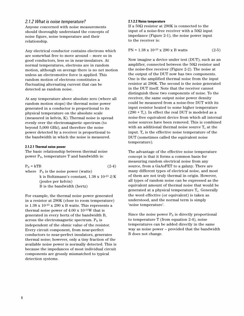
2.1.2.2 Noise temperatureIf a 50Ω resistor at 290K is connected to the input of a noise-free receiver with a 50Ω inputimpedance (Figure 2-1), the noise power input to the receiver is:

PN = 1.38 x 10-23 x 290 x B watts (2-5)

Now imagine a device under test (DUT), such as anamplifier, connected between the 50Ω resistor andthe noise-free receiver (Figure 2-2). The noise atthe output of the DUT now has two components.One is the amplified thermal noise from the input resistor at 290K. The second is the noise generatedin the DUT itself. Note that the receiver cannot distinguish these two components of noise. To thereceiver, the same output noise power densitycould be measured from a noise-free DUT with itsinput resistor heated to some higher temperature(290 + Te). In effect the real DUT is modeled as anoise-free equivalent device from which all internalnoise sources have been removed. This is combinedwith an additional thermal noise source Te at theinput. Te is the effective noise temperature of theDUT (sometimes called the equivalent noise temperature).

The advantage of the effective noise temperatureconcept is that it forms a common basis for measuring random electrical noise from anysource, from a GaAsFET to a galaxy. There aremany different types of electrical noise, and mostof them are not truly thermal in origin. However,all types of random noise can be expressed as theequivalent amount of thermal noise that would be generated at a physical temperature Te. Generallythe word effective (or equivalent) is taken asunderstood, and the normal term is simply ‘noise temperature’.

Since the noise power PN is directly proportional to temperature T (from equation 2-4), noise temperatures can be added directly in the sameway as noise power – provided that the bandwidthB does not change.

7

An example of this is calculating the noise performance of a complete receiving system,including the antenna. As a one-port device thatdelivers noise power, an antenna has an effectivenoise temperature TANT. If the receiver is designedto operate from the source impedance of the antenna (commonly 50Ω or 75Ω) TANT can beadded directly to the receiver noise temperatureTRX to give the system noise temperature TSYS:

TSYS = TANT + TRX (2-6)

This analysis using noise temperatures providesuseful insights into the overall system perform-ance, and can demonstrate whether TSYS is dominated by TANT (which usually cannot bechanged) or by TRX (which often can be improved).Note that such an analysis is not possible usingnoise figure. This is because the fundamental definition of noise figure cannot apply to a one-port device such as an antenna.

The noise temperature concept also has to be usedin the correction of noise figure measurements forresistive losses before or after the device undertest (Sections 4.1 and 4.2).

Noise measuring receiver

50ΩT = 290K

Noise measuring receiver

50ΩT = 290K

Same noise power

Noiseless DUT

Real DUT

Figure 2-1 A resistor at any temperature above absolute zero willgenerate thermal noise.

Figure 2-2 Effective noise temperature is the additional temperature ofthe resistor that would give the same output noise power density as anoiseless DUT.

8

2.1.3 Noise figure in multi-stage systemsThe noise figure definition outlined in Section 2.1.1 may be applied to individual components,such as a single transistor, or to complete multi-stage systems such as a receiver.1 The overall noise figure of the system can be calculatedif the individual noise figures and gains of the system components are known.

Figure 2-3 shows how the noise builds up in a two-stage system. The input noise source is shownas a resistor at the reference temperature T0

(290K). Each stage is characterized by its band-width B, gain G and the noise Na that it adds. The system noise factor F12 is then given by:

F12 = F1 + [(F2 - 1)/G1] (2-7)

(See Application Note 57-1 for the detailed derivation.)

Notice that the bandwidth B has canceled fromequation (2-7). This demonstrates one of theadvantages of the noise figure and noise tempera-ture concept: it is independent of bandwidth.2

The quantity [(F2 -1)/G1] in equation (2-7) is oftencalled the second stage contribution. If the firststage gain G1 is high, that will make the secondstage contribution small so that F12 will be mostlydetermined by F1 alone. This is why a low-noisereceiver almost invariably begins with a low-noise,high-gain RF amplifier or preamplifier.

Equation (2-7) can be re-written to find F1 if all theother quantities are known:

F1 = F12 - [(F2 - 1)/G1] (2-8)

The same equation in terms of noise temperature is:

T1 = T12 - T2/G1 (2-9)

Equations (2-8) and (2-9) are the basis for mostautomatic noise figure analyzers and similar measurement instruments. The device under test(DUT) is always ‘Stage 1’ and the instrumentationconnected to the DUT output is ‘Stage 2’ (Figure 2-4).

2.2 Y-factor measurementThe Y-factor technique is the most commonmethod of measuring the quantities required by equations (2-8) or (2-9) to calculate the noisefactor F1 of the DUT.

This section begins by defining two importantquantities: the Excess Noise Ratio (ENR) of a noise source, and the Y-factor itself.

Sections 2.2.3 through 2.2.7 then explain how thecomplete Y-factor measurement is made.

Figure 2-3. How noise builds up in a two-stage system.

1. Note that noise figure of a receiving system can only extend to the receiver input – it does not include the antenna. See What is noise temperature? (2.1.2) for explanation.2. Unless the bandwidth changes within the system being measured (see Section 3.7)

9

2.2.1 Excess Noise Ratio (ENR)The Y-factor technique involves the use of a noisesource that has a pre-calibrated Excess Noise Ratio(ENR). This is defined as:

ENR = (TSON - TS

OFF) / T0 (2-10)

or more commonly in decibel terms as:

ENRdB = 10 log10 [(TSON - TS

OFF) / T0] (2-11)

TSON and TS

OFF are the noise temperatures of thenoise source in its ON and OFF states. T0 is the reference temperature of 290K that appears in thedefinition of noise figure (equation 2-3).

This definition of ENR supersedes an earlier definition, ENR = [(TS

ON - T0) / T0], which implicitly assumed that TS

OFF was always 290K.The new definition clarifies the fact that TS

OFF

and T0 are usually two different temperatures.Even so, the calibrated ENR of a noise source isalways referenced to TS

OFF = T0 = 290K. Sections3.10 and 4.4 explain how to correct for the common situation where TS

OFF is higher or lowerthan the reference temperature.

2.2.2 Y-factorY-factor is a ratio of two noise power levels, onemeasured with the noise source ON and the otherwith the noise source OFF:

Y = NON/NOFF (2-12)

Because noise power is proportional to noise temperature, it can be stated:

Y = TON/TOFF (2-13)

The instruments mentioned above are designed tomeasure Y-factor by repeatedly pulsing the noisesource ON and OFF. NON and NOFF are thereforemeasured several times, so that an averaged value of Y can be computed.

Figure 2-4. Noise figure measurement uses a two-stage system.

10

2.2.3 CalibrationThe complete Y-factor measurement of DUT noisefigure and gain consists of two steps, as shown inFigure 2-5.

The first step is called calibration (Figure 2-5a)and is done without the DUT in place. The noisesource is usually connected directly to the input of the instrument.3

If the noise temperature of the instrument (stage 2) is T2 then, according to equation (2-12),the Y-factor measured by connecting the noisesource directly to its input will be:

Y2 = N2ON / N2

OFF = (TSON + T2) / (TS

OFF + T2) (2-14)

or

T2 = (TSON - Y2TS

OFF) / (Y2 - 1) (2-15)

TSOFF is the physical temperature of the noise

source, and TSON is computed from the noise

source ENRdB using equation (2-11).

At the end of calibration, the instrument stores the measured values of N2

ON and N2OFF, and the

computed values of Y2 and T2. It then normalizesits noise figure and gain displays to 0 dB, ready for the next step involving the DUT.

2.2.4 Measurement with DUTNext, the DUT is inserted (Figure 2-5b) and the Y-factor measurement is repeated. The system now comprises the DUT (stage 1) followed by the instrument (stage 2) as shown in Figure 2-4.The combined Y-factor Y12 is given by:

Y12 = N12ON / N12

OFF (2-16)

Following equation (2-15), the combined noise temperature T12 of the DUT followed by the instrument is given by:

T12 = (TSON - Y12TS

OFF) / (Y12 - 1) (2-17)

Figure 2-5. The Y-factor noise figure measurement requires two steps: (a) Calibration, (b) Measurement of DUT.

(a) Calibration

(b) Measurement

Noise source

Noise source

DUT

3. The calibration step is comparable to the normalization step when using a network analyzer – before the DUT is inserted, the instrument first ‘measures itself.’

Measurement reference plane

11

2.2.5 Calculation of gainSince the instrument now has values for N12

ON andN12

OFF as well as the previously stored values forN2

ON and N2OFF it can compute the gain of the DUT:

G1 = (N12ON - N12

OFF) / (N2ON - N2

OFF) (2-18)

Usually the instrument displays G1 in dB:

G1,dB = 10 log10G1 dB (2-19)

2.2.6 Second stage correctionThe instrument has now measured T2, T12 and G1.Equation (2-9) has determined that:

T1 = T12 - T2/G1 (2-9)

The instrument now has all the information itneeds to compute T1, the noise temperature of theDUT, corrected for the noise contribution of theinstrument itself.

Most automatic (computing) noise figure instru-ments can display the results in terms of eithernoise temperature T (in K), noise factor F (ratio)or noise figure NF (in dB). The conversions aremade using equations (2-1), (2-2) and (2-3).

2.2.7 SummaryThis section has described in some detail the measurements and internal computations carriedout by an automatic noise figure instrument thatuses the Y-factor method. This information willhelp in understanding the information covered inthe next three chapters:

• Avoidable measurement errors (Chapter 3)

• Loss and temperature corrections (Chapter 4)

• Calculating unavoidable uncertainties (Chapter 5).

12

3 Avoidable measurement errorsThis chapter explains:

• Common errors to avoid when making noise figure measurements

• Routine precautions to minimize common errors

• Practical hints

3.1 Prevent interfering signalsAs explained in Chapter 2, all noise figure instruments measure a sequence of different RFnoise power levels. Any RF interference, eitherradiated or conducted, will masquerade as noisepower and affect measurement accuracy.Interfering RF signals can cause errors of any size in noise figure and gain. Small errors mayescape unnoticed unless an operator is alert to the possibility of interference.

Figure 3-1 shows the kinds of stray signals thatcould be coupled into the signal path and affect the measurement. Fluorescent lights, nearbyinstruments and computers, two-way radios, cellular telephones, pocket pagers and local TV orradio transmitters can all interfere with accuratenoise measurements.

The path by which RF interference enters themeasurement system can be either:

• Direct radiation, with voltages and currents being induced by the electrostatic, magnetic or electromagnetic field.

• Conduction through signal, power, and control cables.

Measurements on receiver components are especially vulnerable to interference from thetransmitters they are designed to receive. Forexample, if testing a cellular telephone receiver,check particularly for interference from cellularphones and base stations nearby. A frequency-swept measurement is more likely to reveal interference than a single-frequency measurement.This is because the sweep often shows clear anomalies at frequencies where interference ispresent. The interference may also change betweensweeps, so that measurements seem to be unstableat certain frequencies only. Once the possibility of interference has been identified, a spectrumanalyzer or a receiver can be used to investigatemore closely.

Figure 3-1. Avoid these interference sources that can affect noise figure measurements.

13

To avoid interference problems, check the following items:

• Use threaded connectors in the signal path whenever possible. (Non-threaded connectors such as BNC or SMB have lower contact forces on the outer shield, which may affect shielding integrity.)

• Ensure that mating connectors are clean and notworn or damaged. Ensure that readings remain stable when lightly shaking the cables and connectors.

• Use double shielded coaxial cables (some regularcoaxial cables have inadequate shielding for these sensitive measurements). Try to avoid using flexible cables at the interface where the signal levels are lowest. If the DUT has gain, connect the noise source directly to its input. If the DUT has loss, connect its output directly to the input of the measurement instrument.

• Use shielded GP-IB cables to prevent radiation or pickup of interference from the control network.

• Avoid making measurements on an open PC breadboard. Use shielding, especially if there is a nearby transmitter that has any output within the measurement bandwidth.

• Relocate the whole setup to a screened room if the DUT and measurement system cannot be shielded adequately on an open bench. It may benecessary to attenuate stray signals as much as 70 to 80 dB.

• Skip over the frequencies of discrete interfering signals when making a swept NF measurement, if the instrumentation and the measurement protocol allow.

• Avoid interference from the instrument itself by using a noise figure analyzer with low RF emissions.4

3.2 Select the appropriate noise sourceNoise sources are available to cover frequencies upto 50 GHz and beyond, with choices of waveguideor co-axial connectors. Most commercial noisesources are supplied with a calibration table ofENR values at specific frequencies.

The ENR calibration uncertainties vary over thefrequency range of the noise source, and will contribute to the overall uncertainty in the noisefigure measurement – often almost dB-for-dB (see Chapter 5).

For high quality noise sources this uncertainty isabout ±0.1dB, which is adequate for most purposes.Noise sources can be specially calibrated to reducethis uncertainty. This is not a cost-effective optionuntil all other possibilities for reducing uncertaintyhave been considered.

3.2.1 Frequency coverage• Use a noise source whose calibration covers the

frequency of the measurement.

The ENR of a well designed noise source changesonly gradually with frequency, and there are nomarked resonances, so linear interpolationbetween calibrated frequencies is acceptable.

If the DUT is a mixer or other frequency-convertingdevice, the noise source should preferably coverboth the input frequency and the output frequencyof the DUT. A full-featured noise figure analyzerwill select the correct ENR data for the calibrationand measurement steps.

If one noise source cannot cover both frequencies,the calibration step and the DUT measurementstep must use two different noise sources. The difference in ENR must be accounted for. Someautomatic noise figure instruments can make thiscorrection but may need to be ‘told’ when thenoise source has been changed.5

4. Agilent Technologies has designed the NFA Series of instruments so that RF emissions from the instrument itself can have little or no impact on the NF measurement. The instruments are also highly immune to radiated or conducted RF interference – except, of course, through the INPUT port.

5. The latest generation of noise sources , identify themselves to the instrument automatically, and upload their own individual ENR table to the instrument. These noise sources operate with noise figure analyzers such as the NFA Series and ESA-E Series spectrum analyzers.

14

3.2.2 Identity checkIf more than one noise source is available, checkthat the noise figure instrument is using the correct ENR calibration table.5

3.2.3 Use low ENR whenever possibleNoise sources are commonly available with nominal ENR values of 15dB and 6dB.

Use a 6dB ENR noise source to measure noise figures up to about 16-18dB, and particularly to minimize measurement uncertainties if:

• The DUT noise figure is very low; and/orthe gain of the device is especially sensitive to changes in the noise source impedance.

A low ENR noise source has the following advantages:

• If the device noise figure is low enough to be measured with a 6dB ENR noise source, the noise power levels inside the noise figure instrument will be lower. This reduces potential errors due to instrument non-linearity (see Section 3.6).

• The impedance match between the noise source and the DUT changes slightly when the source is switched between ON and OFF. The noise output and gain of some active devices (especially GaAsFETs) are particularly sensitive to changes in input impedance. This can cause errors in both gain and noise figure measurement. The 6dB ENR noise sources contain a built-in attenuator that both reduces the ENR and limits the changes in reflection coefficient between ON and OFF states. Section 3.4.2 gives more details.

• The instrument’s own noise figure is a significant contributor to the overall measure-ment uncertainty (see Chapters 2 and 5). The lower the instrument’s internal noise figure, the lower the uncertainty. Many automatic noise figure instruments will insert internal attenuators to handle higher noise input levels. This attenuation will increase the instrument’s noise figure. With a low ENR noise source, the instrument will use less internal attenuation, which will minimize this part of the measurement uncertainty.

Avoid overdriving the instrument beyond its calibrated input range when using a 6dB ENRnoise source with a DUT that has very high gain.

A noise figure instrument that is not auto-rangingcan be driven into non-linearity by a DUT withvery high gain. This results in the measurementerrors described in Section 3.6.1.

Auto-ranging noise figure instruments are less vulnerable to this problem because they automati-cally insert internal attenuators if necessary. Aminor problem is that a low ENR noise sourcemight not allow the instrument to self-calibrate onall of its internal attenuation ranges. If the DUThas more than about 40dB gain, the instrumentmay have to use higher attenuation ranges thathave not been calibrated.6

In both cases, the solution is still to use the lowENR noise source, but to insert a fixed attenuatorafter the DUT to reduce its gain. This attenuatormust not be included in the calibration loop; itmust be accounted for separately (see Section 4.2for details).

3.2.4 When NOT to use low ENRDo not use a 6dB ENR noise source for measurement of noise figures significantly above 16dB. Use a 15dB ENR source instead.

When the DUT noise figure is high and the noisesource ENR is low, the difference in noise levelsbetween the noise source ON and OFF becomesvery small and difficult to measure accurately.This affects the instrument uncertainty(δNFInstrument in Section 5.3, Step 4) in a way that isdifficult to quantify. Also, very long averagingtimes are needed to prevent jitter from making asignificant contribution to the overall measuringuncertainty (see Section 3.5).

There is no sharp limit on DUT noise figure whereuncertainty suddenly becomes excessive. Accuracydeteriorates progressively with increasing difference between the DUT noise figure and the noise source ENR.

6. The Agilent Technologies NFA series noise figure analyzers indicate this condition on the display.

15

A noise source is suitable for accurate measure-ment of noise figures up to about (ENR + 10)dB,with increasing care as this level is approached or exceeded. Thus a 6dB ENR source is generallycapable of good accuracy in measuring noise figures up to about 16dB, and a 15dB ENR source up to about 25dB.

If the DUT noise figure is 15dB above the ENR, orhigher, measurement accuracy is likely to be poor.

3.2.5 Avoid adaptersThe calibrated ENR of a noise source is quoted atits output connection plane. If it is necessary touse adapters between the noise source and theDUT, a correction must be applied for the adapterlosses at the input of the DUT (Section 4.1). Anyuncertainty in the value of this correction will contribute dB-for-dB to the overall measurementuncertainty. It is always preferable to obtain anoise source with the correct connector to matedirectly to the DUT.

3.3 Use a preamplifier where necessaryThis recommendation is closely related to choosingthe appropriate noise source. It applies particularlyto spectrum analyzers that are used with a noisefigure measurement personality.7 This personalitycan convert a spectrum analyzer into a highly effective noise figure analyzer, except that theinstrument noise figure of a spectrum analyzer issignificantly higher than that of a modern purpose-built noise figure analyzer. Therefore, if a spectrumanalyzer is being used to measure low noise figures

using a low ENR noise source, it will generallyrequire a low-noise preamplifier to minimize measurement uncertainties.8

A preamplifier may also be needed with oldernoise figure meters that have a relatively highinstrument noise figure, or with other instrumentsthat can be used to measure noise power level (see Application Note 57-1 for more informationabout these alternative techniques).

A noise figure analyzer that has a low internalnoise figure will not require an external preampli-fier unless the DUT has an unfavorable combina-tion of low noise figure and low gain. Section 6.5will explain how to calculate the uncertaintieswith or without a preamplifier, and hence how to decide whether the preamplifier is needed.

3.4 Minimize mismatch uncertaintiesMismatch at any interface plane will create reflections of noise power in the measurementpath and the calibration path (as shown in Figure 3-2). Mismatch uncertainties will combinevectorially and will contribute to the total measurement uncertainty.

The best measurement technique is to minimize all avoidable mismatch uncertainties, and then use the information in Chapter 5 to account for the uncertainties that remain.

Figure 3-2. Example of mismatch effects.

7. For example, the Agilent Technologies ESA-E Series and PSA Series spectrum analyzers with noise figure measurement personality.8. For example, the Agilent Technologies option 1DS for the PSA Series or ESA-E Series when working below 3GHz.

16

3.4.1 Use an isolator or attenuator padAn isolator is a one-way device that transmits incident RF power with only a small insertion loss,but absorbs any reflected power in a matched load.Placing an isolator between the noise source andthe DUT can prevent reflections from reaching thenoise source where they could reflect again andcombine with the incident signal. Isolators, however,operate over restricted frequency ranges. A wide-band frequency-swept measurement may need tobe stopped several times to change isolators, and acontinuous frequency sweep will not be possible.Also, each isolator has its own frequency-dependentinput/output mismatch and insertion loss.Therefore each isolator must be accurately characterized using a network analyzer, and frequency-dependent corrections applied in thenoise figure calculation (see Section 4.1).9

Another method to reduce mismatch between thenoise source and the DUT is to insert a resistiveattenuator pad between the two. This has the effectof attenuating reflections each time they passthrough the pad. For example, a perfectly matched10dB attenuator will have a return loss of 20dB forreflected signals.10 Unlike an isolator, a resistiveattenuator has the advantage of broadbandresponse. The disadvantage is that an attenuatorreduces the ENR of the noise source (as seen bythe DUT) by its insertion loss. To avoid ENR uncertainties, the insertion loss of the attenuatormust therefore be accurately characterized acrossthe required frequency range, and a correctionapplied in the noise figure calculation (see Section 4.1).9

A better alternative, where possible, is to use a lowENR noise source which has a built-in attenuatorwhose effects are already included in the ENR calibration (see Section 3.2.3). In this case, no losscorrection is required.

3.4.2 Minimize change in ρ of noise sourceSome low-noise devices (notably GaAsFETs) have aparticularly high input reflection coefficient. Evena small change in the output reflection coefficientof the noise source between its ON and OFF conditions can cause significant errors in themeasured noise figure. Even worse, if the input

circuit of a low noise amplifier is being adjusted to the minimum noise figure, changes in noisesource reflection coefficient can result in a falseminimum. To minimize these effects, an attenuatorpad or isolator must be used between the noisesource and the DUT. Fortunately, low-noise devicesare best measured using a low ENR noise source,which already contains a built-in attenuator.

No correction for the change in noise source reflection coefficient is possible without extremelydetailed information about the effects of inputreflections on the noise and gain performance ofthe DUT. Usually, the only workable strategy is tominimize the changes.

3.4.3 Measures of mismatchThere are several ways to express how well an RF impedance is matched to the system designimpedance (usually 50Ω but sometimes some otherresistive impedance such as 75Ω). The four common quantities used are VSWR, reflection coefficient, return loss and the S-parameters S11

or S22. RF engineers tend to use these terms interchangeably, depending on the type of deviceor the network property they wish to emphasize.11

3.4.3.1 VSWR: voltage standing wave ratio

This relates to the standing wave that is formed on a transmission line by the interaction betweenthe forward and reflected travelling voltage waves.VSWR is literally VMAX / VMIN for the standing wave.At suitable frequencies, VSWR can be measureddirectly by a slotted-line probe in either a coaxialline or waveguide. Alternatively a bridge or directional coupler can resolve the forward and reflected waves on the line (VFWD and VREFL) and then:

VSWR = (VFWD + VREFL) / (VFWD - VREFL) (3-1)

VSWR is ideally 1 on a matched line, and greaterthan 1 in practice. VSWR is a scalar quantity – it describes the magnitude of a mismatch but contains no information about the phase.

9. The Agilent Technologies analyzers with noise figure capability have a loss compensation facility to correct for losses between the noise source and the input of the DUT.

10. See section 3.4.3: Measures of mismatch.11. ‘S-Parameter Design’, Agilent Technologies Application Note 154, March 1990 (5952-1087). and ‘S-Parameter Techniques for Faster, More Accurate

Network Design’, Agilent Technologies Application Note 95-1, 1996 (5952-1130); also available as Agilent Interactive Application Note 95-1, http://www.tm.agilent.com/data/static/eng/tmo/Notes/interactive/an-95-1/

17

3.4.3.2 Reflection coefficientReflection coefficient ρ (the Greek letter rho) isdefined simply as lVREFL / VFWDl, so:

VSWR = (1 + ρ) / (1 - ρ) or (3-2)

ρ = (VSWR - 1) / (VSWR +1) (3-3)

ρ is a scalar quantity that is ideally zero on amatched line and greater than zero in practice. The quantity (VREFL / VFWD) is the complex reflec-tion coefficient Γ (the Greek capital letter gamma);it is a vector quantity with both magnitude andassociated phase angle.

3.4.3.3 Return lossReturn loss is the ratio in dB of forward and reflected power:

RLdB = -10 log10(PREFL / PFWD) = -20 log10(VREFL / VFWD) = -20 log10(ρ) (3-4)

The higher the return loss, the better the impedance match. Return loss from an ideallymatched line is infinite. A return loss of 0dB represents total reflection from a complete mismatch. Return loss can either be a scalar quantity or a vector quantity.

3.4.3.4 S-parametersS (scattering) parameters are a method of describing the behavior of incident and reflectedwaves at the ports of a network. In a two-port network, S11 is the input reflection coefficient andS22 is the output reflection coefficient (S21 is theforward transfer parameter, and S12 describes the reverse transfer). S-parameters are almostinvariably measured as vector quantities with bothmagnitude and an associated phase angle, so S11

and S22 are complex reflection coefficients like Γ.

3.4.4 Mismatch-related errorsInsertion loss can generally be divided into two parts:

• Dissipative (resistive) loss• Reflection (mismatch) loss.

In noise figure measurements, dissipative mechanisms are recognized as a source of bothinsertion loss and thermal noise (Sections 4.1-4.3).Reflection mechanisms do not generate thermalnoise, but they are a source of uncertainty. This isbecause scalar measurements of insertion loss andVSWR (or reflection coefficient) cannot predicthow the vector reflection coefficients will combinewhen two imperfectly matched components areconnected.

One approach, taken in some network analyzersthat also have the capability of noise figure measurement, is to measure the vector mismatchesand apply a correction. Unfortunately this is not afull correction because it overlooks an extremelyimportant fact: the mismatch changes the actualnoise figure of the DUT. To make a valid correctionfor mismatch errors, it is necessary to know howthe DUT noise figure is affected by a range of complex source and load impedances.

Neither a noise figure analyzer nor a network analyzer with noise figure capability can generatethis information on its own. It requires a special-ized automated test set that uses stub tuners topresent the DUT with a range of complex imped-ances and incorporates a noise figure analyzer tomap the effects on gain and noise figure. As shownin Figure 3-3, a test set can generate a Smith chart showing circular contours of noise figure in thecomplex impedance. It is important to note thatnoise figure contours are almost never centered on the 50Ω reference impedance at the center ofthe chart or on the conjugate match to the deviceinput impedance.

18

Without the complete map of noise figure contours – which cannot be measured by a network analyzer – there is no way to be sure that the correction for a vector impedance mismatch will actually decrease the error of themeasurement. The error could even be increased.

It is invalid to attempt mismatch corrections for noise figure measurements made using either a noise figure analyzer or a network analyzer with noise figure capability. Instead, impedancemismatch should be minimized in the design of themeasurement, and any residual mismatch shouldproperly be treated as an uncertainty (Chapter 5).Designers of modern noise figure analyzers haveconcentrated on minimizing all other sources of measurement uncertainty so that the total uncertainty budget can almost always be reducedto acceptably low values.

In uncommon cases where mismatch errors areboth unavoidable and significant, the only effectivesolution requires full mapping of noise figure contours in the complex impedance plane using atest set such as one available from ATN Microwave(www.atnmicrowave.com).

3.5 Use averaging to avoid display jitterNoise is a result of a series of random independentelectrical events. In principle, the time required tofind the true mean noise level would be infinite.Noise measurement captures a finite series ofthese random events within the measurementbandwidth, and therefore the results inherentlydisplay random fluctuations or jitter. Averagingmany readings over an extended time period willreduce the displayed jitter, and bring the resultcloser to the true long-term mean.

There is a trade-off between reduction of jitter and the measurement time required. To obtain asufficiently accurate result, a suitable number ofreadings must be averaged. Most computing noisefigure instruments have a facility for automaticdigital averaging over a selected number of inter-nal readings (N), generally displaying a ‘rolling’average over the last N readings.

Assuming that the noise being measured has agaussian probability distribution, averaging of Nreadings will decrease the jitter by the square rootof N. As shown in the table below, by averaging 10readings the jitter can be reduced to about 30% ofthe value for a single reading (see Table 3-1).

Figure 3-3 The noise figure of most devices depends on the input impedance presented to the device. Without full knowledge of the noise figure contours on a Smith chart, mismatch corrections can be uncertain and may introduce more error.

19

As explained in Section 3.7, it is sometimes necessary to make measurements in a reducedbandwidth. In that case, the number of readingsaveraged must be proportionally increased in orderto achieve the same level of jitter. For example, ifthe bandwidth is reduced from 4MHz to 100kHz (a factor of 40), readings must be averaged for 40times as long to achieve the same level of jitter.

If speed is not the first priority (e.g. in an R&Denvironment) the instrument should generally be set to average sufficient readings to make theresidual jitter a minor component of the overallmeasurement uncertainty (see Chapter 5). If speedis a high priority (e.g. in a production environ-ment) and the number of readings is low enough to leave a significant uncertainty due to jitter, a jitter contribution must be added to the overallmeasurement uncertainty.

Jitter in the calibration step will add to the uncertainty of all subsequent measurements.Therefore a long averaging time should be used for calibration in order to reduce this source ofuncertainty to a negligible level. This is an efficient use of time because it benefits all subsequent measurements.

In frequency-sweep mode, two modes may be available for updating the display while averaging is taking place.12 ‘Point averaging’ takes all the nec-essary readings for each frequency before averaging them and then moving on to the next frequency. The average at each frequency is notdisplayed until the measurement at that frequencyis complete. ‘Trace averaging’ takes one reading ateach frequency across the whole frequency sweep,and then repeats the whole sweep as many timesas necessary, updating the display as it goes. Bothmodes of averaging give the same result. Traceaveraging quickly displays a rough measurementover the entire frequency range. Point averaging isfaster overall because the analyzer does not haveto change frequency after each reading.

Use trace averaging first. Watch a few sweepsacross the display and look for indications of RFinterference such as a spike in the response at asingle frequency, or even a small step in theresponse. If there are no problems, change to point averaging for faster measurements.

12. The Agilent Technologies NFA Series noise figure analyzers have both averaging modes.

Number of readings averaged % reduction

(N) √(N) in jitter % residual jitter

1 1 0 100

4 2 50.0 50.0

10 3.16 68.4 31.6

16 4 75.0 25.0

64 8 87.5 12.5

100 10 90.0 10.0

256 16 93.75 6.25

Table 3-1

20

3.6 Avoid non-linearity or unstable performance

Accurate noise figure measurements rely on thelinearity and stability of the entire measurementsystem. This includes both the DUT and the noisefigure instrument itself.

3.6.1 Non-linearityAvoid operating either the DUT or the noise figure instrument in a situation that would causenon-linear behavior. In particular:

• Do not attempt to measure devices that are specifically designed to be non-linear, such as logarithmic amplifiers or limiting amplifiers. Thetechniques described in this Application Note are not suitable for such devices. Similarly, do not attempt to measure devices that need an input signal in order to operate correctly (e.g. systems that phase-lock to an input signal); these require specialist techniques to measure noise figure.

• Avoid operating the DUT near its saturated output power level where limiting occurs. Accurate measurements require less than 0.05dBgain difference between the ON and OFF states of the noise source.

• Disable any AGC circuits in the DUT, and take manual control of the gain to establish the required conditions for the measurement. Be aware that AGC-controlled amplifiers may have alimited linear range when operated without AGC.Also, some systems control the gain by techniques that can themselves introduce non-linearity. If applying a temporary control voltage, do not introduce hum or noise that will modulate the gain.

• Do not attempt to measure circuits that self-oscillate or feed significant levels of local oscillator leakage through to the noise figure instrument; these will cause either RF inter-ference or non-linearity. Even if far removed from the measurement frequency, all signals of this type should be regarded as RF interference (see Section 3.1) and either suppressed within the DUT or removed by an external filter.

• Use a low ENR noise source whenever the DUT noise figure is low enough to be measured accurately with such a source (see Section 3.2). The noise power levels inside the noise figure instrument will be lower, which reduces potential errors due to instrument non-linearity.

• Insert in-line attenuation after a DUT with high gain to avoid driving the noise figure instrument beyond its linear range. The instrument specifica-tion will indicate the maximum total gain that can be handled between the noise source and theinstrument’s input. If attenuation is needed afterthe DUT, it must be accurately characterized using a network analyzer and a correction must be applied in the noise figure calculation (Section 4.2).13

3.6.2 Unstable performanceTo avoid unstable or drifting performance, use regulated power supplies for the DUT. Allow theDUT and the noise figure instrument to warm upand stabilize before starting measurements.

Consider keeping a ‘reference’ device that can bemeasured at the beginning of each day. This willverify that the same result is obtained as on previousdays as well as confirm that the measurementinstrument is warmed up and has stabilized.

13. The Agilent Technologies analyzers with noise figure capability have a loss compensation facility to correct for losses between the output of the DUT and the input port of the instrument. As already noted, there is a separate compensation facility for losses between the noise source and the input of the DUT.

21

Figure 3-4 A narrowband DUT can cause errors. Use a resolution bandwidth narrower than the bandwidth of the DUT.

3.7 Choose the appropriate measurement bandwidth

The typical internal bandwidth of a noise figureinstrument is 3–4 MHz. Errors can arise if the DUTcontains filters that have a narrower bandwidththan the instrument itself. During calibration theinstrument measures the total noise power withinits own internal bandwidth. However, during themeasurement the bandwidth is restricted by theDUT (see Figure 3-4). This causes an error in theDUT gain measurement, which affects the correction for the instrument’s own noise figure (Section 2.2.6).

The error becomes insignificant if the gain of the DUT is high enough to be several orders ofmagnitude greater than the ratio of the band-widths during calibration and DUT measurement.The DUT gain criterion is therefore:

[GDUT, dB] >> [10 log10(BCALIBRATION / BMEASUREMENT)] (3-5)

If the DUT gain criterion cannot be met, choose aresolution bandwidth that is significantly less thanthe bandwidth of the DUT. Take into account thepossibility of relative drift between the two passbands during the measurement. Both the calibration and the measurement must use thesame bandwidth.

The modern full-featured NFA Series noise figureanalyzer, with digital signal processing, allows theresolution bandwidth to be reduced from the IFbandwidth of 4MHz down to 100kHz. A PSA Seriesor ESA Series spectrum analyzer with the noisefigure measurement personality also has the facilityto reduce the IF bandwidth down to 1 Hz/1 kHzrespectively.

Alternatively, a suitably narrow bandpass filter canbe inserted between the DUT and the input of thenoise figure instrument. The instrument shouldthen be calibrated with the filter in place. Theinsertion loss of the filter, however, will increasethe effective noise figure of the instrument. It maybe necessary to use a low-noise preamplifier toavoid introducing new sources of uncertainty (see Section 3.3).

Whichever technique is used for reducing band-width, it will always increase the averaging timerequired to achieve the same low level of jitter (see Section 3.5). This is because the number ofrandom noise events being averaged is reduced in proportion to the bandwidth.14

14. For swept-frequency measurements with narrow bandwidth, the Agilent Technologies NFA Series noise figure analyzers can make blocks of simultaneous measurements in adjacent channels that cover a total of almost 4MHz. The necessary averaging time remains the same for each channel, but the simultaneous measurement feature can often reduce the time required for the complete frequency sweep.

22

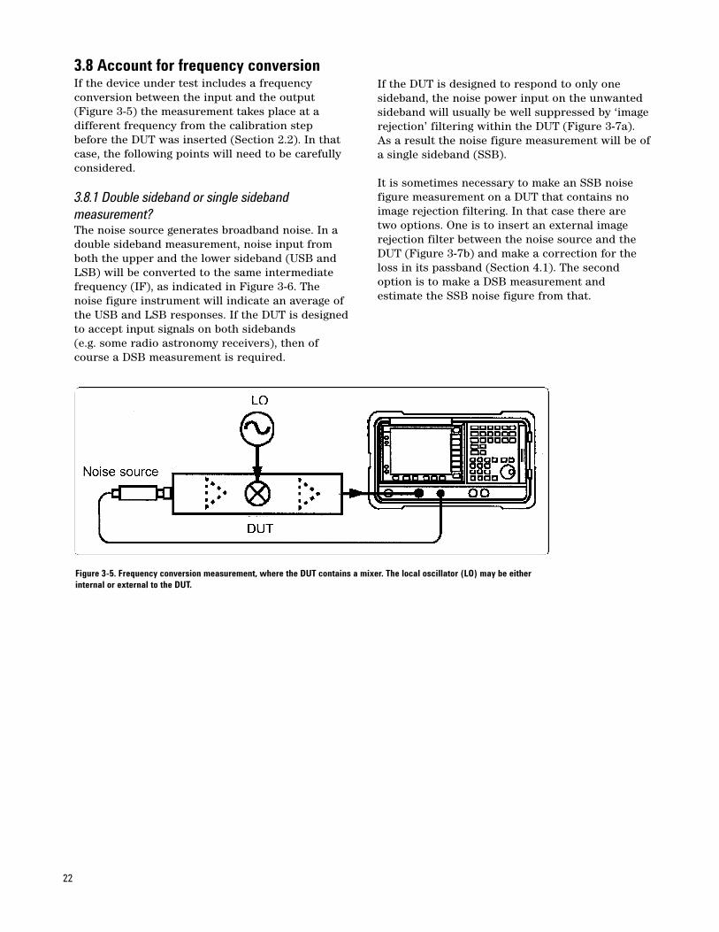
3.8 Account for frequency conversionIf the device under test includes a frequency conversion between the input and the output(Figure 3-5) the measurement takes place at a different frequency from the calibration stepbefore the DUT was inserted (Section 2.2). In thatcase, the following points will need to be carefullyconsidered.

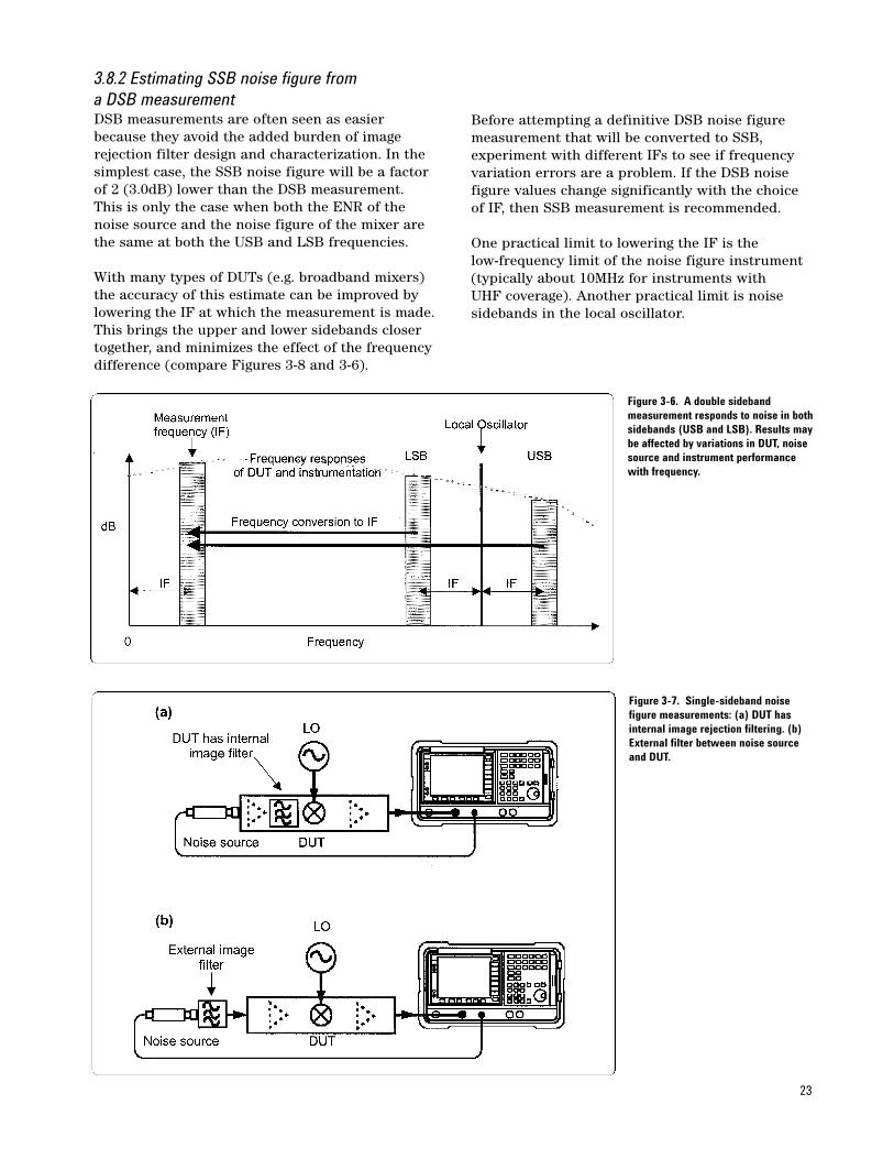
3.8.1 Double sideband or single sideband measurement?The noise source generates broadband noise. In adouble sideband measurement, noise input fromboth the upper and the lower sideband (USB andLSB) will be converted to the same intermediatefrequency (IF), as indicated in Figure 3-6. Thenoise figure instrument will indicate an average ofthe USB and LSB responses. If the DUT is designedto accept input signals on both sidebands (e.g. some radio astronomy receivers), then ofcourse a DSB measurement is required.

If the DUT is designed to respond to only one sideband, the noise power input on the unwantedsideband will usually be well suppressed by ‘imagerejection’ filtering within the DUT (Figure 3-7a). As a result the noise figure measurement will be ofa single sideband (SSB).

It is sometimes necessary to make an SSB noisefigure measurement on a DUT that contains noimage rejection filtering. In that case there are two options. One is to insert an external imagerejection filter between the noise source and theDUT (Figure 3-7b) and make a correction for theloss in its passband (Section 4.1). The secondoption is to make a DSB measurement and estimate the SSB noise figure from that.

Figure 3-5. Frequency conversion measurement, where the DUT contains a mixer. The local oscillator (LO) may be eitherinternal or external to the DUT.

23

Figure 3-7. Single-sideband noisefigure measurements: (a) DUT hasinternal image rejection filtering. (b)External filter between noise sourceand DUT.

Figure 3-6. A double sideband measurement responds to noise in bothsidebands (USB and LSB). Results maybe affected by variations in DUT, noisesource and instrument performancewith frequency.

3.8.2 Estimating SSB noise figure from a DSB measurementDSB measurements are often seen as easierbecause they avoid the added burden of imagerejection filter design and characterization. In thesimplest case, the SSB noise figure will be a factorof 2 (3.0dB) lower than the DSB measurement.This is only the case when both the ENR of thenoise source and the noise figure of the mixer arethe same at both the USB and LSB frequencies.

With many types of DUTs (e.g. broadband mixers)the accuracy of this estimate can be improved bylowering the IF at which the measurement is made.This brings the upper and lower sidebands closertogether, and minimizes the effect of the frequencydifference (compare Figures 3-8 and 3-6).

Before attempting a definitive DSB noise figuremeasurement that will be converted to SSB, experiment with different IFs to see if frequencyvariation errors are a problem. If the DSB noisefigure values change significantly with the choiceof IF, then SSB measurement is recommended.

One practical limit to lowering the IF is the low-frequency limit of the noise figure instrument (typically about 10MHz for instruments with UHF coverage). Another practical limit is noisesidebands in the local oscillator.

24

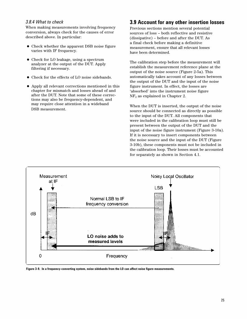
3.8.3 Local oscillator noise and leakageNo oscillator produces a single, pure frequency. In particular, the LO that is used in a noise figuremeasurement with frequency conversion willalways generate noise sidebands on both sides ofthe carrier frequency. Typically the noise sidebandlevel reduces with frequency offset from the carrier,eventually reaching an almost constant noise floorlevel that can be very broadband. As shown inFigure 3-9, high levels of the LO noise sidebands or noise floor may contribute to the measurednoise power and may cause erroneous results.

The importance of LO noise entering the noise figure instrument will depend on several factors:

• The noise sideband level (measured in dBc/Hz, i.e. relative to the carrier level and normalized toa 1Hz bandwidth). The noise sideband power density is a function of:

- the LO design, and many of its operatingparameters, especially level and frequency

- the IF, which is the offset between the measurement frequency and the LO frequency;the smaller this offset, generally the higher is the noise sideband level

- the measurement bandwidth.

• The broadband noise floor level.

• The mixer’s LO to IF port isolation. A well-balanced mixer may give a rejection of 30dB or better for LO noise sidebands, but non-balanced mixer configurations may have zero LO-IF isolation.

• The noise figure and gain of the DUT.

As a general rule, the LO noise level at the IF separation from the carrier should not exceed -130dBm/Hz. More specifically:

[LO power level (dBm) - LO phase noise suppression (dBc/Hz)] should not exceed[ -174 dBm/Hz + expected NF (dB) + Gain of DUT (dB)] (3-6)

Another important factor is the level of LO leakage through the DUT and into the noise figureinstrument. As noted in Sections 3.1 and 3.6, thiscan cause errors by appearing as RF interferenceand/or by overdriving the instrument into anuncalibrated or non-linear region.

Figure 3-8. Reducing the IF for a DSB measurement can also reduce the effect of differences in noise figure (and/or ENR of noise source)between the LSB and USB. Compare against Figure 3-5.

25

Figure 3-9. In a frequency-converting system, noise sidebands from the LO can affect noise figure measurements.

3.8.4 What to checkWhen making measurements involving frequencyconversion, always check for the causes of errordescribed above. In particular:

• Check whether the apparent DSB noise figure varies with IF frequency.

• Check for LO leakage, using a spectrum analyzer at the output of the DUT. Apply filtering if necessary.

• Check for the effects of LO noise sidebands.

• Apply all relevant corrections mentioned in thischapter for mismatch and losses ahead of and after the DUT. Note that some of these correc-tions may also be frequency-dependent, and may require close attention in a wideband DSB measurement.

3.9 Account for any other insertion lossesPrevious sections mention several potentialsources of loss – both reflective and resistive (dissipative) – before and after the DUT. As a final check before making a definitive measurement, ensure that all relevant losses have been determined.

The calibration step before the measurement willestablish the measurement reference plane at theoutput of the noise source (Figure 2-5a). This automatically takes account of any losses betweenthe output of the DUT and the input of the noisefigure instrument. In effect, the losses are‘absorbed’ into the instrument noise figure NF2 as explained in Chapter 2.

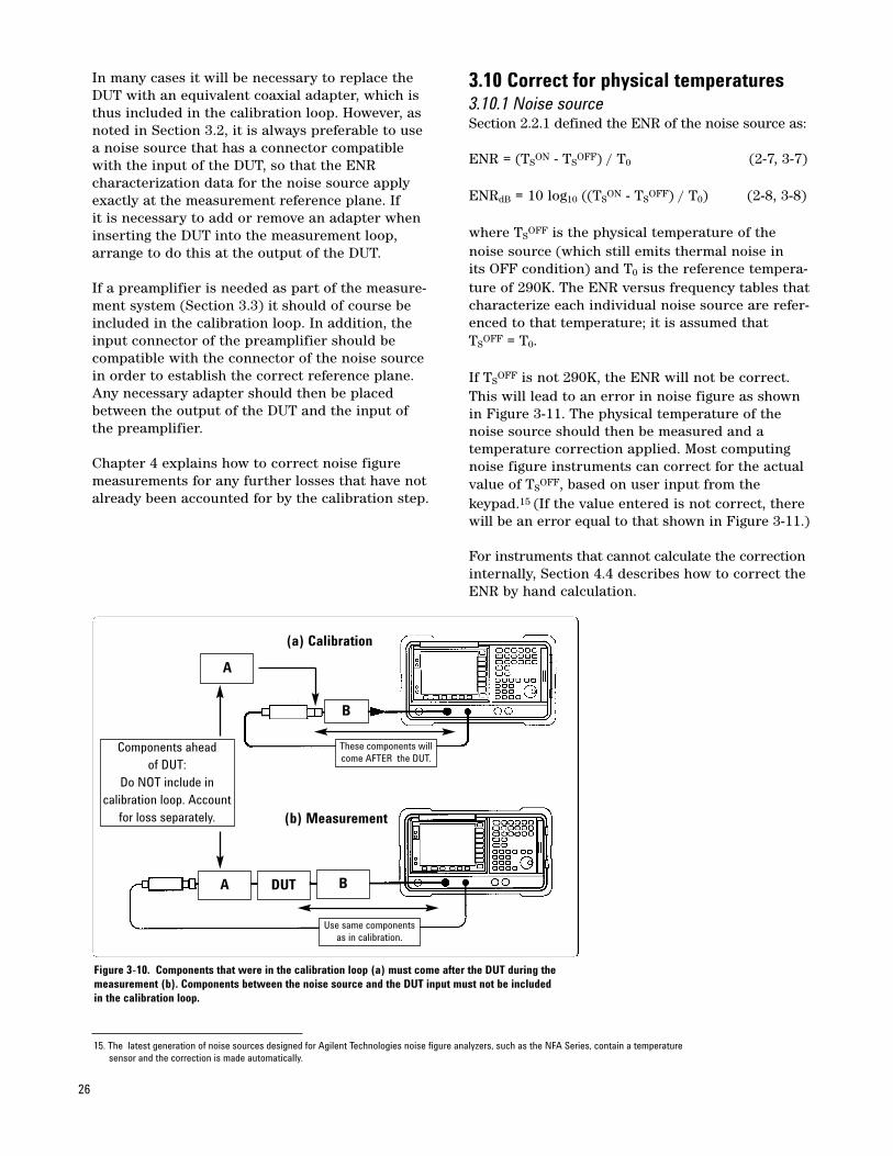
When the DUT is inserted, the output of the noisesource should be connected as directly as possibleto the input of the DUT. All components that were included in the calibration loop must still bepresent between the output of the DUT and theinput of the noise figure instrument (Figure 3-10a).If it is necessary to insert components between the noise source and the input of the DUT (Figure3-10b), these components must not be included inthe calibration loop. Their losses must be accountedfor separately as shown in Section 4.1.

26

In many cases it will be necessary to replace theDUT with an equivalent coaxial adapter, which isthus included in the calibration loop. However, asnoted in Section 3.2, it is always preferable to usea noise source that has a connector compatiblewith the input of the DUT, so that the ENR characterization data for the noise source applyexactly at the measurement reference plane. If it is necessary to add or remove an adapter wheninserting the DUT into the measurement loop,arrange to do this at the output of the DUT.

If a preamplifier is needed as part of the measure-ment system (Section 3.3) it should of course beincluded in the calibration loop. In addition, theinput connector of the preamplifier should be compatible with the connector of the noise sourcein order to establish the correct reference plane.Any necessary adapter should then be placedbetween the output of the DUT and the input ofthe preamplifier.

Chapter 4 explains how to correct noise figuremeasurements for any further losses that have notalready been accounted for by the calibration step.

3.10 Correct for physical temperatures3.10.1 Noise sourceSection 2.2.1 defined the ENR of the noise source as:

ENR = (TSON - TS

OFF) / T0 (2-7, 3-7)

ENRdB = 10 log10 ((TSON - TS

OFF) / T0) (2-8, 3-8)

where TSOFF is the physical temperature of the

noise source (which still emits thermal noise in its OFF condition) and T0 is the reference tempera-ture of 290K. The ENR versus frequency tables thatcharacterize each individual noise source are refer-enced to that temperature; it is assumed that TS

OFF = T0.

If TSOFF is not 290K, the ENR will not be correct.

This will lead to an error in noise figure as shownin Figure 3-11. The physical temperature of thenoise source should then be measured and a temperature correction applied. Most computingnoise figure instruments can correct for the actualvalue of TS

OFF, based on user input from the keypad.15 (If the value entered is not correct, therewill be an error equal to that shown in Figure 3-11.)

For instruments that cannot calculate the correctioninternally, Section 4.4 describes how to correct theENR by hand calculation.

Figure 3-10. Components that were in the calibration loop (a) must come after the DUT during themeasurement (b). Components between the noise source and the DUT input must not be includedin the calibration loop.

(a) Calibration

(b) Measurement

A DUT B

Use same components as in calibration.

Components ahead of DUT:

Do NOT include in calibration loop. Account

for loss separately.

A

B

These components willcome AFTER the DUT.

15. The latest generation of noise sources designed for Agilent Technologies noise figure analyzers, such as the NFA Series, contain a temperature sensor and the correction is made automatically.

3.10.2 Noise generated in resistive lossesAny components in the test setup that have resistive losses (attenuators, cables etc.) will generate thermal noise in their own right. Thissource of temperature-related error is often overlooked. As well as allowing for the loss itself, a complete correction needs to take account of thenoise generation in the components involved. Thisin turn requires measurement of their physicaltemperatures. Sections 4.1 and 4.2 show how tomake the corrections.

Corrections for physical temperature do not applyto the DUT itself. Its physical temperature isassumed to be part of the DUT test conditions, sothe measured noise figure and gain are applicableat that physical temperature.

4 Loss and temperature corrections

This chapter explains how to make corrections for the residual errors due to losses, either aheadof or following the DUT. Closely related to this is the correction for the physical temperature of the noise source and the temperature of lossy components.

The equations for the corrections are given interms of noise temperature because that is theparameter most directly affected. For more information on noise temperature, see Chapter 2.

All of the corrections described in this chapter arefrequency-dependent. Frequency-swept measure-ments may need a table of corrections versus frequency. A modern full-featured noise figure analyzer has the capability to make the correctionsdescribed in this chapter automatically if it is supplied with frequency-dependent tables of loss data.

27

Figure 3-11. Magnitude of error in noise figure measurement if TSOFF is not 290K. If the noise figure

instrument can correct for the actual value of TSOFF an equal error arises if the value input to the

instrument is not correct.

28

4.1 Losses before the DUTThe reference plane for the ENR characterizationof the DUT is the output of the noise source(Figure 2-5a). Any additional losses between thatreference plane and the input of the DUT must betaken into consideration..

Section 2.2 derived the equation to calculate thenoise temperature T1 of the DUT, with a correctionfor the ‘second stage’ contribution from the instrument itself (T2/G1):

T1 = T12 - T2/G1 (2-6, 4-1)

For this loss correction, the ‘input’ loss LIN needsto be expressed as a ratio greater than 1, so that:

LIN = antilog10(LINdB/10) (4-2)

The correction for input loss changes the originalvalue of T1 to T1

IN. If the input loss ahead of theDUT is LIN (as a ratio greater than 1, not dB) then:

T1IN = [T1/LIN] - [(LIN - 1)TL/LIN] (4-3)

where T1 is the original displayed value of noisetemperature, and T1

IN is the new value correctedfor input losses.

Equation (4-3) has two terms. The first representsthe direct effect of LIN upon T1. The second term isthe added noise contribution from thermal noise inany resistive loss at a physical temperature TL. IfLIN is purely reflective (non-dissipative) in character, omit the second term.

4.2 Losses after the DUTAs noted in Sections 3-9 and 3-10, correction for‘losses after the DUT must only be applied to com-ponents that had not been included in the calibra-tion loop (Figure 3-10). For output losses thecorrection is to T2, the noise temperature of theinstrument (as already modified by componentsincluded in the calibration loop).

T2OUT = [T2/LOUT] - [(LOUT - 1)TL/LOUT] (4-4)

As in equation (4-2), LOUT is a ratio greater than 1 and TL is the physical temperature of anydissipative losses. Once again, if LOUT is purelyreflective (non-dissipative) in character, omit thesecond term.

The modified value T2OUT is inserted into

equation (4-1) to calculate a new value of T1OUT,

which is the original value of T1 corrected for output losses:

T1OUT = T12 - T2

OUT/G1 (4-5)

4.3 Combined correctionsThe separate corrections for input and output losses can of course be combined to give T1

IN, OUT

which is the value of T1 after both corrections havebeen applied:

T1IN, OUT = T12 - [T2 / LOUT - (LOUT - 1) TL / LOUT]

/G1 / LIN - (LIN - 1) TL / LIN (4-6)

A modern full-featured noise figure analyzer has the capability to make these corrections automatically if it is supplied with frequency-dependent tables of loss data.

4.4 Temperature of noise sourceContinuing from Section 3.10.1, if TS

OFF is not290K, the physical temperature of the noise sourceshould be measured and the following temperaturecorrection applied.

ENRCORR = ENRCAL + [(T0 - TSOFF) / T0] (4-7)

ENRdBCORR = 10 log10 [antilog10[ENRdB

CAL / 10] + [(T0 - TS

OFF) / T0] (4-8)

where

• ENRCORR, ENRdBCORR are the corrected

ENR values (ratio or dB, respectively)

• ENRCAL, ENRdBCAL are the original

calibrated ENR values (ratio or dB, respectively)

• TSOFF is the actual physical temperature of the

noise source (K)

• T0 is 290K.

29

Figure 5-1 Model for uncertainty calculation.

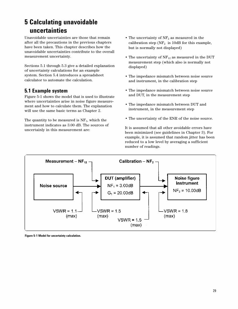
5 Calculating unavoidable uncertainties

Unavoidable uncertainties are those that remainafter all the precautions in the previous chaptershave been taken. This chapter describes how theunavoidable uncertainties contribute to the overallmeasurement uncertainty.

Sections 5.1 through 5.3 give a detailed explanationof uncertainty calculations for an example system. Section 5.4 introduces a spreadsheet calculator to automate the calculation.

5.1 Example systemFigure 5-1 shows the model that is used to illustratewhere uncertainties arise in noise figure measure-ment and how to calculate them. The explanationwill use the same basic terms as Chapter 2.

The quantity to be measured is NF1, which theinstrument indicates as 3.00 dB. The sources ofuncertainly in this measurement are:

• The uncertainty of NF2 as measured in the calibration step (NF2 is 10dB for this example, but is normally not displayed)

• The uncertainty of NF12 as measured in the DUT measurement step (which also is normally not displayed)

• The impedance mismatch between noise source and instrument, in the calibration step

• The impedance mismatch between noise source and DUT, in the measurement step

• The impedance mismatch between DUT and instrument, in the measurement step

• The uncertainty of the ENR of the noise source.

It is assumed that all other avoidable errors havebeen minimized (see guidelines in Chapter 3). Forexample, it is assumed that random jitter has beenreduced to a low level by averaging a sufficientnumber of readings.

30

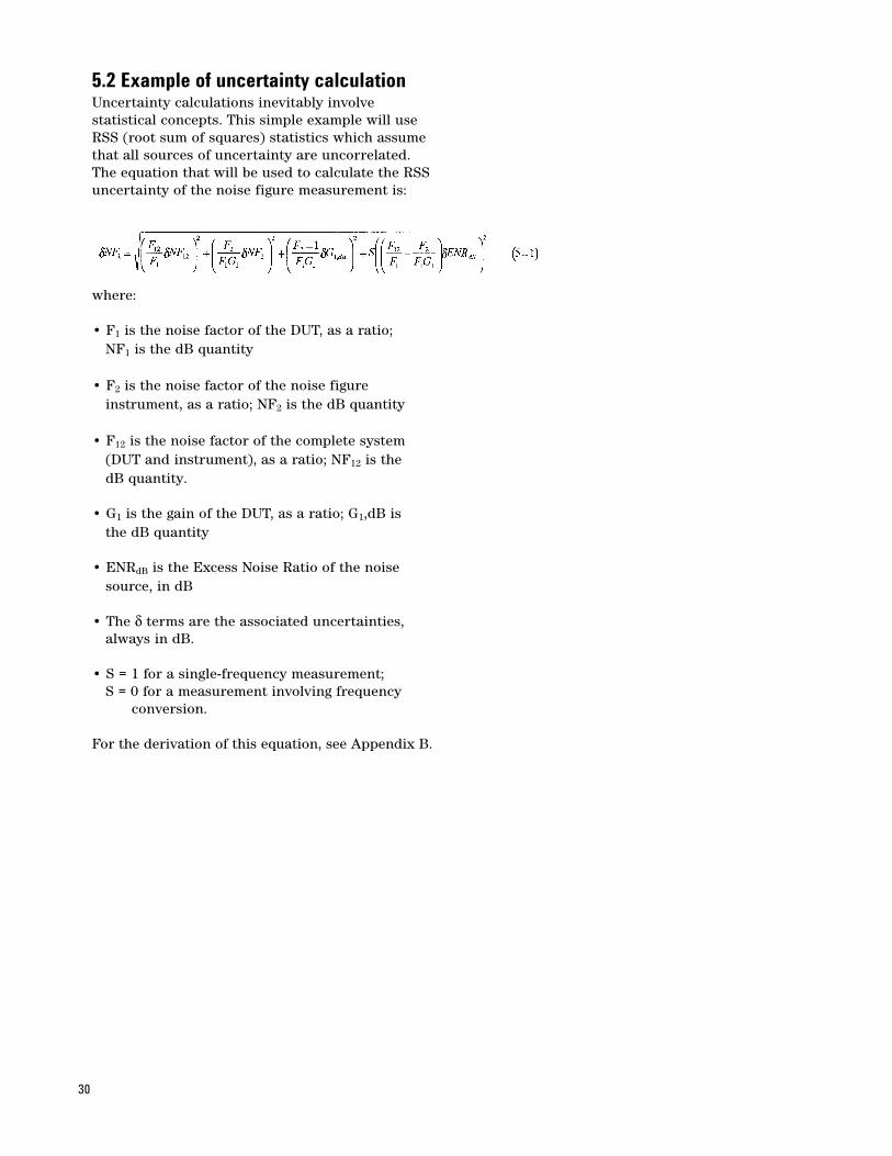
5.2 Example of uncertainty calculationUncertainty calculations inevitably involve statistical concepts. This simple example will useRSS (root sum of squares) statistics which assumethat all sources of uncertainty are uncorrelated.The equation that will be used to calculate the RSSuncertainty of the noise figure measurement is:

where:

• F1 is the noise factor of the DUT, as a ratio; NF1 is the dB quantity

• F2 is the noise factor of the noise figure instrument, as a ratio; NF2 is the dB quantity

• F12 is the noise factor of the complete system (DUT and instrument), as a ratio; NF12 is the dB quantity.

• G1 is the gain of the DUT, as a ratio; G1,dB is the dB quantity

• ENRdB is the Excess Noise Ratio of the noise source, in dB

• The δ terms are the associated uncertainties, always in dB.

• S = 1 for a single-frequency measurement; S = 0 for a measurement involving frequency

conversion.

For the derivation of this equation, see Appendix B.

31

5.3 Step by stepThis section works through the uncertainty calculation, step by step. This is usually done by a computer. However, when learning about theprocess it is valuable to explore the reasoningbehind each step.

Check boxes like this will mark each practical operation. An automatic (computing) noise figure instrument is assumed.

Step 1 – Measurements Referring to the user documentation for a noise

figure instrument, calibrate the instrument (thiswill zero the noise figure and gain displays).

Insert the DUT and measure the DUT gain (G1) and corrected DUT noise figure (NF1)

Determine NF2, the noise figure of the instru-ment. Because the instrument normalizes its noise figure and gain displays to zero after the calibration step, this would not normally be displayed. To gain access to NF2, switch off the instrument’s auto-ranging with the DUT still in place; this will lock the internal attenuators in their present settings. Remove the DUT and repeat a calibration-type measurement. The instrument will now display its own internal noise figure NF2.

Step 2 – Calculate noise figure and gain quantities Convert all the dB values into linear equivalents

and insert them into the table below:

• NF12,dB ⇒ noise factor F12

• NF2,dB ⇒ noise factor F2

• G1,dB ⇒ gain ratio G1

Also calculate F12 as shown in the following table:

RatioQuantity dB = antilog10(dB/10)

F1 3 1.995F2 10 10G1 20 100F12 = F1 + (F2-1)/G1 3.19 2.085

Calculate the following quantities, for later use in Step 5:

Quantity Value

F12 / F1 1.045F2 / F1G1 0.050(F2-1) / F1G1 0.045(F12/F1) - (F2/F1G1) 0.995

Step 3 – Calculate mismatch uncertainties Convert the maximum VSWR at each interface

into a reflection coefficient (ρ). Use either measured values or the maximum values quotedin the instrument specifications.

Calculate the various matching uncertainties, based on the reflection coefficients.

• The negative uncertainty is equal to:

–20 log(1-ρSourceρLoad) dB

• The positive uncertainty is equal to:

+20 log(1+ρSourceρLoad) dB

• Choose whichever of the two is the greater (underlined).

Interface VSWR Reflection Coefficientρ= (VSWR-1) / (VSWR+1)

Noise source output 1.1 0.048DUT input 1.5 0.200

DUT output 1.5 0.200Instrument input 1.8 0.286

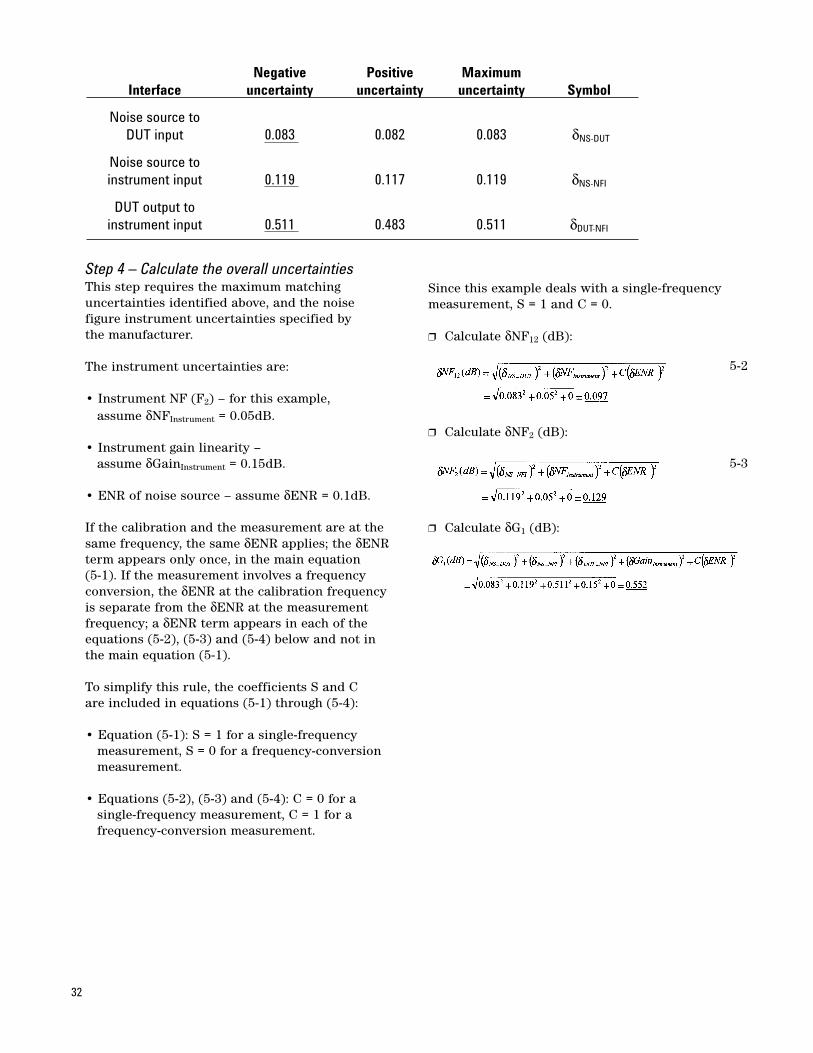
32

Step 4 – Calculate the overall uncertaintiesThis step requires the maximum matching uncertainties identified above, and the noise figure instrument uncertainties specified by the manufacturer.

The instrument uncertainties are:

• Instrument NF (F2) – for this example, assume δNFInstrument = 0.05dB.

• Instrument gain linearity – assume δGainInstrument = 0.15dB.

• ENR of noise source – assume δENR = 0.1dB.

If the calibration and the measurement are at thesame frequency, the same δENR applies; the δENRterm appears only once, in the main equation (5-1). If the measurement involves a frequency conversion, the δENR at the calibration frequencyis separate from the δENR at the measurement frequency; a δENR term appears in each of theequations (5-2), (5-3) and (5-4) below and not inthe main equation (5-1).

To simplify this rule, the coefficients S and C are included in equations (5-1) through (5-4):

• Equation (5-1): S = 1 for a single-frequency measurement, S = 0 for a frequency-conversion measurement.

• Equations (5-2), (5-3) and (5-4): C = 0 for a single-frequency measurement, C = 1 for a frequency-conversion measurement.

Since this example deals with a single-frequencymeasurement, S = 1 and C = 0.

Calculate δNF12 (dB):

Calculate δNF2 (dB):

Calculate δG1 (dB):

Negative Positive MaximumInterface uncertainty uncertainty uncertainty Symbol

Noise source to DUT input 0.083 0.082 0.083 δNS-DUT

Noise source to instrument input 0.119 0.117 0.119 δNS-NFI

DUT output to instrument input 0.511 0.483 0.511 δDUT-NFI

5-2

5-3

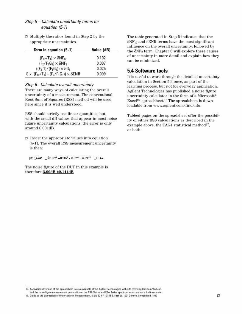
33

Step 5 – Calculate uncertainty terms for equation (5-1)

Multiply the ratios found in Step 2 by the appropriate uncertainties.

Term in equation (5-1) Value (dB)

(F12/F1) × δNF12 0.102(F2/F1G1) × δNF2 0.007

((F2-1)/(F1G1)) × δG1 0.025S x ((F12/F1) - (F2/F1G1)) × δENR 0.099

Step 6 - Calculate overall uncertaintyThere are many ways of calculating the overalluncertainty of a measurement. The conventionalRoot Sum of Squares (RSS) method will be usedhere since it is well understood.

RSS should strictly use linear quantities, but with the small dB values that appear in most noisefigure uncertainty calculations, the error is onlyaround 0.001dB.

Insert the appropriate values into equation (5-1). The overall RSS measurement uncertainty is then:

The noise figure of the DUT in this example istherefore 3.00dB ±0.144dB

The table generated in Step 5 indicates that theδNF12 and δENR terms have the most significantinfluence on the overall uncertainty, followed bythe δNF2 term. Chapter 6 will explore these causesof uncertainty in more detail and explain how theycan be minimized.

5.4 Software toolsIt is useful to work through the detailed uncertaintycalculation in Section 5.3 once, as part of thelearning process, but not for everyday application.Agilent Technologies has published a noise figureuncertainty calculator in the form of a Microsoft®Excel™ spreadsheet.16 The spreadsheet is down-loadable from www.agilent.com/find/nfu.

Tabbed pages on the spreadsheet offer the possibil-ity of either RSS calculations as described in theexample above, the TAG4 statistical method17, or both.

16. A JavaScript version of the spreadsheet is also available at the Agilent Technologies web site (www.agilent.com/find/nf), and the noise figure measurement personality on the PSA Series and ESA Series spectrum analyzers has a built-in version.

17. Guide to the Expression of Uncertainty in Measurement, ISBN 92-67-10188-9, First Ed. ISO, Geneva, Switzerland, 1993

34

5.4.1 RSS calculationsFigure 5-2 shows the spreadsheet in use for thesame RSS uncertainty calculation as detailed inSection 5.3. The uncertainty result is of course the same as in the hand calculation.

Enter the input data in the outlined yellow cells onthe spreadsheet. Compare Figures 5-1 and 5-2 tosee where to enter each item. In the “ImpedanceMismatch” area, the spreadsheet will correctlyinterpret numerical entries in the form of VSWR(≥1), reflection coefficient (<1) or return loss (negative, no dB units required).

If the box labeled Frequency-converting DUT? ischecked, the spreadsheet ensures that the ENRuncertainty is applied correctly. This is equivalentto changing coefficients S and C in equations (5-1)through (5-4).

5.4.2 TAG4 calculationsThe RSS method of calculation assumes that all the random variables are uncorrelated. This isprobably correct, but is normally an unverifiedassumption. The TAG4 method17 offers potentiallymore accurate estimation of uncertainties by calcu-lating and using any correlations that are present.The disadvantage of the TAG4 method is that a fullimplementation requires data from several sets ofreadings in order to extract the correlations.

The Agilent Technologies noise figure uncertaintycalculator offers a simplified method of TAG4 cal-culation, using statistically justifiable assumptionsto calculate standard uncertainties and covariancewhen multiple data sets are not available. In mostcases the RSS and simplified TAG4 results will bealmost identical – compare Figures 5-2 and 5-3.

The data for the TAG4 calculation are entered inthe same way as for the RSS calculation (Figure 5-2). A third tabbed page on the spreadsheet givesthe results from both methods from the same set of input data.

Agilent Technologies will continue to developmethods of uncertainty calculation for noise figuremethods, so it is advisable to check the web siteperiodically.

5.5 Effects of loss corrections on uncertaintyThe loss corrections described in Chapter 4 willintroduce further uncertainties of their own.

The uncertainty in correcting for the input loss LIN (Section 4.1) will add directly to δENR, the calibration uncertainty of the noise source.The uncertainty in correcting for the output lossLOUT (Section 4.2) will add directly to the gainuncertainty δG, and also to the instrument noisefigure uncertainty δNF2. If the DUT has significantgain, both of these terms will be small.

35

Figure 5-2. Spreadsheet for the RSS uncertainty calculation using the example in Sections 5.1–5.3.

Figure 5-3. An alternative manner to obtain the result would be to utilize the noise figurespreadsheet calculator. Using the same data as Figure 5-2 both methods provide thesame results, and both methods can be found at http://www.agilent.com/find/nfu. The difference being that the noise figure uncertainty calculator can be used to providegraphic results allowing a number of the modeled parameters to be swept, while thespreadsheet provides all the information on a single page.

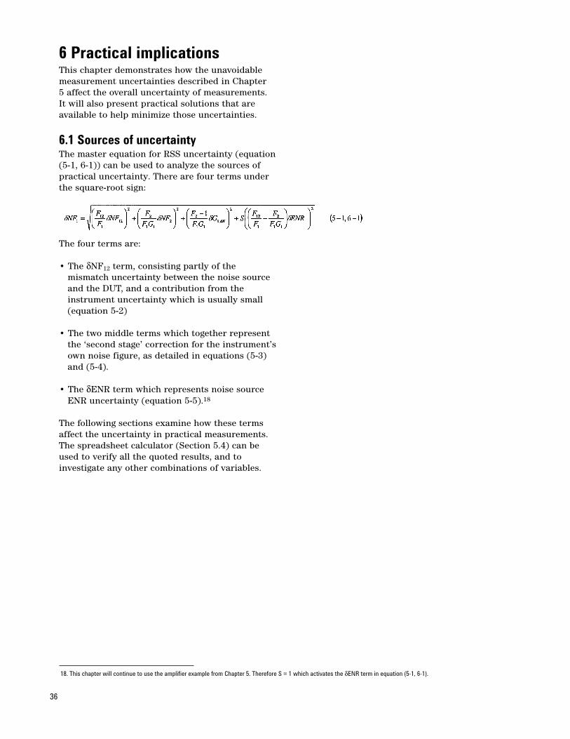
36

6 Practical implicationsThis chapter demonstrates how the unavoidablemeasurement uncertainties described in Chapter 5 affect the overall uncertainty of measurements. It will also present practical solutions that areavailable to help minimize those uncertainties.

6.1 Sources of uncertaintyThe master equation for RSS uncertainty (equation(5-1, 6-1)) can be used to analyze the sources ofpractical uncertainty. There are four terms underthe square-root sign:

The four terms are:

• The δNF12 term, consisting partly of the mismatch uncertainty between the noise source and the DUT, and a contribution from the instrument uncertainty which is usually small (equation 5-2)

• The two middle terms which together represent the ‘second stage’ correction for the instrument’sown noise figure, as detailed in equations (5-3) and (5-4).

• The δENR term which represents noise source ENR uncertainty (equation 5-5).18

The following sections examine how these termsaffect the uncertainty in practical measurements.The spreadsheet calculator (Section 5.4) can beused to verify all the quoted results, and to investigate any other combinations of variables.

18. This chapter will continue to use the amplifier example from Chapter 5. Therefore S = 1 which activates the δENR term in equation (5-1, 6-1).

37

Figure 6-1. Uncertainty versus instrument NF and instrument errors (DUT gain 10dB, other variables atdefault values used in spreadsheet).

6.2 Instrument noise figure and instrument errors

In cases where the second-stage correction isimportant, usually because the DUT gain is low, the instrument’s own noise figure can make a significant contribution to the overall uncertainty.In equation (5-1, 6-1) this appears mostly in theuncertainty term δNF2.

Figure 6-1 shows a typical trend of uncertaintyincreasing with the instrument noise figure (note that the overall uncertainty is shown on anunusual log-decibel scale to expand the detail atlower values). Figure 6-1 uses mostly the defaultvalues in the spreadsheet calculator. This meansthat the minimum possible uncertainty is deter-mined largely by the ENR uncertainty of 0.1dB,plus combined mismatch uncertainties of about0.04dB. The spreadsheet calculator can be used to investigate other combinations of parameter values.

The main conclusion from Figure 6-1 is that a high instrument noise figure can be a significantcontribution to the total uncertainty. The solutionsto this are either to use an instrument with a lowernoise figure, or to reduce the instrument noise figure by means of a low-noise preamplifier. There

are limits however to the effectiveness of the preamplifier solution. This will as will beaddressed in more detail in Section 6.5. Figure 6-1 shows that the noise figure instrument’sown errors are almost always a small part of thetotal uncertainty. In equation (6-1) these errorsappear mostly in the δNF12 term. The main sourcesof instrument errors are:

• In the measurement of noise figure, first during calibration and then when measuring the DUT.

• In the measurement of gain, which is also used in the correction for the instrument noise figure.

The solid curve in Figure 6-1 represents the ideal-ized case where instrument errors are zero. Thecurve marked ‘Spreadsheet default’ is for typicalerror levels in a modern noise figure instrument(0.05dB in noise figure, 0.15dB in gain). Comparingthe ‘Spreadsheet default’ curve against the ‘Zero errors’ curve, the contribution to the totaluncertainty is almost negligible. The third curve isfor doubled values of those two instrument errors.Even with this pessimistic assumption the contribution to the total uncertainty is small.

38

Figure 6-2. 3-D plot of typical RSS uncertainty versus DUT noise figure and gain.

6.3 Uncertainty versus DUT noise figure and gain

Figure 6-2 shows how the RSS uncertainty of a typical noise figure measurement depends on thenoise figure and gain of the DUT. The data werederived using the noise figure spreadsheet, usingthe default values for the other parameters.

The 3-D surface in Figure 6-2 has a large region oflow uncertainty where the DUT noise figure andgain are both reasonably high. The uncertaintyincreases when both of these parameters are low.In the most favorable region, the uncertainty isdominated by:

• The δENR term which represents noise source ENR uncertainty (equation (5-5).

• The δNF12 term in equation (5-1, 6-1). Equation (5-2) shows this is partly due to the mismatch uncertainty between the noise source and the DUT, with a generally small contribution from instrument errors.

In the most favorable region of Figure 6-2, the twomiddle terms in equation (5-1, 6-1) are relativelysmall. Together these two terms represent the ‘second stage’ correction for the instrument noisefigure, as detailed in equations (5-3) and (5-4). Thissituation represents almost the lowest uncertaintyachievable, since it is difficult to improve on thetwo remaining terms, δNF12 and δENR.

If the DUT gain G1 is quite high (e.g. 20dB), thetotal uncertainty remains quite low, down to verylow values of DUT noise figure. However, if G1 islow, the uncertainty increases dramaticallybecause the second-stage correction grows larger.All the terms in equation (5-1, 6-1), especially the δG1 term, will then increase. In extreme casesthe uncertainty can even exceed the measuredvalue of noise figure, so these regions are clearly to be avoided.

6.4 A possible solution – re-define the ‘DUT’

There is sometimes a very simple solution to the problem of low gain in the DUT– change the definition of ‘what is the DUT’.

For example, if a diode ring mixer (with negativegain) is always followed by an IF preamplifier,uncertainties can be reduced by making the measurement on the combined module rather than the low-gain mixer on its own.

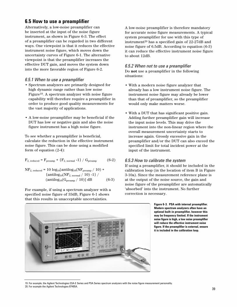
39

6.5 How to use a preamplifierAlternatively, a low-noise preamplifier can be inserted at the input of the noise figure instrument, as shown in Figure 6-3. The effect of a preamplifier can be regarded in two differentways. One viewpoint is that it reduces the effectiveinstrument noise figure, which moves down theuncertainty curves of Figure 6-1. The alternativeviewpoint is that the preamplifier increases theeffective DUT gain, and moves the system downinto the more favorable region of Figure 6-2.

6.5.1 When to use a preamplifier• Spectrum analyzers are primarily designed for

high dynamic range rather than low noise Figure19. A spectrum analyzer with noise figure capability will therefore require a preamplifier inorder to produce good quality measurements for the vast majority of applications.

• A low-noise preamplifier may be beneficial if the DUT has low or negative gain and also the noise figure instrument has a high noise figure.

To see whether a preamplifier is beneficial, calculate the reduction in the effective instrumentnoise figure. This can be done using a modifiedform of equation (2-4):

F2, reduced = Fpreamp + F2, normal -1 / Gpreamp (6-2)

NF2, reduced = 10 log10[antilog10(NFpreamp / 10) + antilog10(NF2, normal / 10) -1 /(antilog10(Gpreamp / 10)] dB (6-3)

For example, if using a spectrum analyzer with aspecified noise figure of 33dB, Figure 6-1 showsthat this results in unacceptable uncertainties.

A low-noise preamplifier is therefore mandatoryfor accurate noise figure measurements. A typicalsystem preamplifier for use with this type ofinstrument20 has a specified gain of 22-27dB andnoise figure of 6.5dB. According to equation (6-3)it can reduce the effective instrument noise figureto about 12dB.

6.5.2 When not to use a preamplifierDo not use a preamplifier in the following situations:

• With a modern noise figure analyzer that already has a low instrument noise figure. The instrument noise figure may already be lower than that of preamplifier, so the preamplifier would only make matters worse.

• With a DUT that has significant positive gain. Adding further preamplifier gain will increase the input noise levels. This may drive the instrument into the non-linear region where the overall measurement uncertainty starts to increase again. Grossly excessive gain in the preamplifier and/or the DUT can also exceed thespecified limit for total incident power at the input of the instrument.

6.5.3 How to calibrate the systemIf using a preamplifier, it should be included in thecalibration loop (in the location of item B in Figure3-10a). Since the measurement reference plane is at the output of the noise source, the gain andnoise figure of the preamplifier are automatically‘absorbed’ into the instrument. No further correction is necessary.

Figure 6-3. PSA with internal preamplifier.Modern spectrum analyzers often have anoptional built-in preamplifier, however thismay be frequency limited. If the instrumentnoise figure is high, a low noise preamplifierwill reduce the effective instrument noisefigure. If the preamplifier is external, ensureit is included in the calibration loop.

19. For example, the Agilent Technologies ESA-E Series and PSA Series spectrum analyzers with the noise figure measurement personality.20. For example the Agilent Technologies 87405A.

40

6.6 Solutions – reduce ENR uncertaintyThe 0.1dB uncertainty specified for AgilentTechnologies noise sources is adequate for mostmeasurement purposes. For the 346 Series noisesources, the ENR calibration and some of its uncertainty are traceable to the US NationalInstitute of Standards and Technology (NIST).Calibration of the latest generation of noisesources, the SNS Series, designed for the AgilentTechnologies noise figure measuring analyzerssuch as the NFA Series, is traceable to the BritishNational Physical Laboratory (NPL). Both nationalstandards laboratories collaborate to maintainworldwide uniformity of noise power calibrations.

These commercially available noise sources areremoved from NIST or NPL by two or three calibration generations (depending on frequency).Each calibration generation introduces a smalladditional uncertainty.

If the application is especially demanding and all other sources of errors and unavoidable uncertainties are already minimized, then it may be worthwhile to remove some of the ENR uncertainty. Noise source recalibration servicesare available that can typically eliminate one calibration generation, bringing the calibrationcloser to the relevant national standards laboratory.21

21. The Agilent Technologies Standards Laboratory offers such a service (contact the nearest Agilent Technologies service center for details). NPL and NIST also offer commercial calibration services for noise sources (contact those bodies directly).

41

7 Checklist for improving measurement accuracy

Prevent interfering signals (Section 3.1) Use threaded connectors whenever possible. Ensure that mating connectors are clean,

sound and not worn (see Appendix C, Connector care).

Lightly shake all cables and connectors, and ensure that readings remain stable.

Use double shielded coaxial cables. If the DUT has gain, be sure to connect the noise source directly to its input.

Use shielded GP-IB cables to prevent radiation or pickup of interference on the control network.

Avoid making measurements on an open PC breadboard.

Use a screened room if necessary. If allowable, skip over the frequencies of

interfering signals when making a swept NF measurement.

Select the appropriate noise source (Section 3.2) Check frequency coverage. Confirm correct noise source identity. Use a low ENR noise source whenever

possible.

Do not use a low ENR source if the DUT noisefigure is significantly greater than (ENR + 10)dB.

Avoid adapters between the noise source and the DUT

Use a preamplifier where necessary (Section 3.3, 6.5)

Minimize mismatch uncertainties (Section 3.4) Use an isolator or attenuator pad Minimize change in ρ of noise source

Use averaging to avoid display jitter (Section 3.5, 3.7)

Avoid non-linearity or unstable performance (Section 3.6)

Choose the appropriate measurement band-width (Section 3.7)

Account for frequency conversion (Section 3.8) Double sideband or single sideband

measurement?

Check whether the apparent DSB noise figurevaries with IF frequency.

Check for LO leakage, using a spectrum analyzer at the output of the DUT. Apply filtering if necessary.

Check for the effects of LO noise sidebands. Apply all relevant corrections for losses

ahead of and after the DUT. Note that some of these corrections may also be frequency-dependent.

Account for any other insertion losses (Section 3.9, Chapter 4)

Correct for physical temperatures (Section 3.10, Chapter 4)

42

Appendix A: Symbols and abbreviationsThis list includes major symbols only. Other symbols are defined locally where used.

For a complete Glossary of terms related to noisefigure measurement, see Agilent TechnologiesApplication Note 57-1, ‘Fundamentals of RF andMicrowave Noise Figure Measurements’.

AGC Automatic gain control

B Bandwidth (Hz)

C ‘Switch’ coefficient for δENR; 0 or 1

dBc Decibels relative to carrier power

DSB Double sideband

DUT Device under test

ENR Excess noise ratio (power ratio)

ENRdB Excess noise ratio (dB)

F Noise factor (power ratio)

F1 Noise factor (power ratio) of first stage (DUT)

F12 Combined noise factor (powerratio) of cascaded first and second stages (DUT and noise figure instrument)

F2 Noise factor (ratio) of second stage(often noise figure instrument)

G Gain (power ratio)

G1 Gain (power ratio) of first stage (DUT)

G1,dB Gain (dB) of first stage (DUT)

K kelvin (unit of absolute temperature)

k Boltzmann’s constant, 1.38 x 10–23 J/K

LIN / LOUT Losses before the DUT input / after the DUT output

LO Local oscillator

N Noise power

NON / NOFF Noise powers measured when noise source is ON / OFF

NF, NFdB Noise figure (dB)

P Power

PN Noise power

RLdB Return loss (dB)

RSS Root sum of squares

S ‘Switch’ coefficient for δENR; 1 or 0

S11 / S22 Input / output scattering parameters (reflection coefficients)

SSB Single sideband

T, Te Effective (or equivalent) noise temperature

T0 Reference temperature (290K)

T1 Noise temperature of first stage(often DUT)

T1IN T1 corrected for the effects of LIN

(uncalibrated losses between thenoise source and the input of theDUT)

T1OUT T1 corrected for the effects of LOUT

(uncalibrated losses between theoutput of the DUT and the input ofthe noise figure instrument)

T1IN,OUT T1 corrected for the effects of both

LIN and LOUT

T12 Combined noise temperature ofcascaded first and second stages(DUT and noise figure instrument)

T2 Noise temperature of second stage(often noise figure instrument)

TL Physical temperature of a component with dissipative (resistive) loss

TON / TOFF Noise temperatures measured when noise source is ON / OFF

TSON Noise temperature of noise source

in its ON state

TSOFF Noise temperature of noise

source in its OFF state, equal to itsphysical temperature

TAG4 ISO statistical method

VSWR Voltage standing wave ratio

Y Y-factor: ratio of noise power levelswhen noise source is ON / OFF

δ terms Uncertainties associated with therespective quantities (dB) (delta)

Γ Complex reflection coefficient (capital gamma)

ρ Scalar reflection coefficient (rho);magnitude of Γ

43

Appendix B: Derivation of theRSS uncertainty equationThe general equation for the noise figure of twocascaded stages is:

We are interested in the uncertainty of F1, thenoise figure of the DUT, so re-arranging:

Because F1 is dependent on the three independentvariables F12, F2 and G1, Taylor’s Theorem can beapplied to find the uncertainty of F1:

From equation 2:

So:

What is required is an equation which gives theuncertainty relative to F1. To achieve this, all thenoise factors (F, ratio) in Equation 4 are first converted into noise figures (NF, dB) and G1 islikewise converted into dB. The terms in Equation4 can then be manipulated into the desired formusing the following standard differential coefficientfor a log quantity:

Therefore:

Substituting the above into Equation 4 and simplifying:

The three δ terms in Equation 5 are due to thenoise figure instrument and the DUT. However,noise figure instruments rely on a calibrated noisesource with a specified Excess Noise Ratio (ENR).Clearly there will be an uncertainty associatedwith this ENR (δENR) and this will contribute tothe overall uncertainty equation.

If the calibration and the measurement are at thesame frequency, the same δENR applies, so the following term appears in the overall uncertaintyequation 6:

If the measurement involves a frequency conversion,the δENR at the calibration frequency is separatefrom the δENR at the measurement frequency. A single δENR term is no longer possible, so aδENR contribution appears in each of the otherterms instead. See the main text for further details.

Since the causes of the uncertainties in the four d terms are different, the terms can be combinedin a RSS (Root Sum of Squares) fashion, whichgives a realistic overall uncertainty value.The equation for the overall RSS noise figureuncertainty is therefore:

Equation 6 is the source of equations (5-1) and (6-1) in the main text.

(B - 1)

(B - 2)

(B - 3)

(B - 4)

(B - 5)

(B - 6)

Appendix C: Connector care Avoid dirtEven a small amount of dirt on a connector can cause poor contact that will:

• Cause a mismatch• Attenuate wanted signals• Invalidate instrument calibration • Allow interference to enter.

It only takes one dirty connector to spread dirt to many others. If there is visible dirt on a connector, clean it with a cotton swab and isopropyl alcohol.

Avoid damageA damaged connector can cause all the same problems as a dirty one. Likewise, it can spreaddamage to many other connectors, and the onlysolution is replacement.

Avoid wearConnectors do not last forever – they wear, andeventually they wear out. Connectors with wornplating on the mating surfaces of the inner andouter conductors should be replaced before theystart to cause intermittent connections or physicaldamage to other connectors.

With threaded connectors:

Always mate the threads carefully – take care not to spread thread damage to other connectors

Never rotate the body of a component to tighten the connector thread – keep the two component bodies still and rotate only the connector nut.

Always use the correct wrench to tighten a connector nut.

Always finish tightening the connector nut with a torque wrench adjusted to the correct value.

For further information, see ‘Principles ofMicrowave Connector Care (for Higher Reliabilityand Better Measurements)’; Agilent ApplicationNote 326, literature number 5954-1566.

Agilent Technologies’ Test and Measurement Support, Services, and AssistanceAgilent Technologies aims to maximize the value you receive, while minimizing yourrisk and problems. We strive to ensure that you get the test and measurementcapabilities you paid for and obtain the support you need. Our extensive supportresources and services can help you choose the right Agilent products for yourapplications and apply them successfully. Every instrument and system we sell has a global warranty. Support is available for at least five years beyond the production life of the product. Two concepts underlie Agilent’s overall support policy:“Our Promise” and “Your Advantage.”

Our PromiseOur Promise means your Agilent test and measurement equipment will meet itsadvertised performance and functionality. When you are choosing new equipment, we will help you with product information, including realistic performance specifications and practical recommendations from experienced test engineers.When you use Agilent equipment, we can verify that it works properly, helpwith product operation, and provide basic measurement assistance for theuse of specified capabilities, at no extra cost upon request. Many self-help toolsare available.

Your AdvantageYour Advantage means that Agilent offers a wide range of additional expert testand measurement services, which you can purchase according to your unique technical and business needs. Solve problems efficiently and gain a competitiveedge by contracting with us for calibration, extra-cost upgrades, out-of-warrantyrepairs, and onsite education and training, as well as design, system integration,project management, and other professional engineering services. ExperiencedAgilent engineers and technicians worldwide can help you maximize your productivity,optimize the return on investment of your Agilent instruments and systems, andobtain dependable measurement accuracy for the life of those products.

www.agilent.com/find/emailupdatesGet the latest information on the products and applications you select.

Agilent T&M Software and ConnectivityAgilent’s Test and Measurement software and connectivity products, solutions anddeveloper network allows you to take time out of connecting your instruments toyour computer with tools based on PC standards, so you can focus on your tasks,not on your connections. Visit www.agilent.com/find/connectivityfor more information.

By internet, phone, or fax, get assistance with all your test & measurement needs

Online Assistance:www.agilent.com/find/assist

Product specifications and descriptions in this document subject to change without notice.

© Agilent Technologies, Inc. 2001, 2004Printed in USA March 19, 20045952-3706E

Phone or FaxUnited States:(tel) 800 829 4444Canada:(tel) 877 894 4414(fax) 905 282 6495China:(tel) 800 810 0189(fax) 800 820 2816Europe:(tel) (31 20) 547 2323(fax) (31 20) 547 2390Japan:(tel) (81) 426 56 7832(fax) (81) 426 56 7840

Korea:(tel) (82 2) 2004 5004 (fax) (82 2) 2004 5115Latin America:(tel) (305) 269 7500(fax) (305) 269 7599Taiwan:(tel) 0800 047 866 (fax) 0800 286 331Other Asia Pacific Countries:(tel) (65) 6375 8100 (fax) (65) 6836 0252Email: tm_asia@agilent.com

Agilent Email Updates