nineteen dubious ways to compute the exponential of a ....pdf · nineteen dubious ways to compute...
TRANSCRIPT

SIAM REVIEW c© 2003 Society for Industrial and Applied MathematicsVol. 45, No. 1, pp. 3–000
Nineteen Dubious Ways toCompute the Exponential of aMatrix, Twenty-Five YearsLater∗
Cleve Moler†
Charles Van Loan‡
Abstract. In principle, the exponential of a matrix could be computed in many ways. Methods involv-ing approximation theory, differential equations, the matrix eigenvalues, and the matrixcharacteristic polynomial have been proposed. In practice, consideration of computationalstability and efficiency indicates that some of the methods are preferable to others, butthat none are completely satisfactory.Most of this paper was originally published in 1978. An update, with a separate bibliog-raphy, describes a few recent developments.
Key words. matrix, exponential, roundoff error, truncation error, condition
AMS subject classifications. 15A15, 65F15, 65F30, 65L99
PII. S0036144502418010
1. Introduction. Mathematical models of many physical, biological, and eco-nomic processes involve systems of linear, constant coefficient ordinary differentialequations
x(t) = Ax(t).
Here A is a given, fixed, real or complex n-by-n matrix. A solution vector x(t) issought which satisfies an initial condition
x(0) = x0.
In control theory, A is known as the state companion matrix and x(t) is the systemresponse.
In principle, the solution is given by x(t) = etAx0 where etA can be formallydefined by the convergent power series
etA = I + tA +t2A2
2!+ · · · .
∗Published electronically February 3, 2003. A portion of this paper originally appeared in SIAMReview, Volume 20, Number 4, 1978, pages 801–836.
http://www.siam.org/journals/sirev/45-1/41801.html†The MathWorks, Inc., 3 Apple Hill Drive, Natick, MA 01760-2098 ([email protected]).‡Department of Computer Science, Cornell University, 4130 Upson Hall, Ithaca, NY 14853-7501
1

2 CLEVE MOLER AND CHARLES VAN LOAN
The effective computation of this matrix function is the main topic of this survey.We will primarily be concerned with matrices whose order n is less than a few
hundred, so that all the elements can be stored in the main memory of a contemporarycomputer. Our discussion will be less germane to the type of large, sparse matriceswhich occur in the method of lines for partial differential equations.
Dozens of methods for computing etA can be obtained from more or less classicalresults in analysis, approximation theory, and matrix theory. Some of the methodshave been proposed as specific algorithms, while others are based on less constructivecharacterizations. Our bibliography concentrates on recent papers with strong algo-rithmic content, although we have included a fair number of references which possesshistorical or theoretical interest.
In this survey we try to describe all the methods that appear to be practical, clas-sify them into five broad categories, and assess their relative effectiveness. Actually,each of the “methods” when completely implemented might lead to many differentcomputer programs which differ in various details. Moreover, these details might havemore influence on the actual performance than our gross assessment indicates. Thus,our comments may not directly apply to particular subroutines.
In assessing the effectiveness of various algorithms we will be concerned with thefollowing attributes, listed in decreasing order of importance: generality, reliability,stability, accuracy, efficiency, storage requirements, ease of use, and simplicity. Wewould consider an algorithm completely satisfactory if it could be used as the basisfor a general purpose subroutine which meets the standards of quality software nowavailable for linear algebraic equations, matrix eigenvalues, and initial value problemsfor nonlinear ordinary differential equations. By these standards, none of the algo-rithms we know of are completely satisfactory, although some are much better thanothers.
Generality means that the method is applicable to wide classes of matrices. Forexample, a method which works only on matrices with distinct eigenvalues will notbe highly regarded.
When defining terms like reliability, stability and accuracy, it is important todistinguish between the inherent sensitivity of the underlying problem and the errorproperties of a particular algorithm for solving that problem. Trying to find theinverse of a nearly singular matrix, for example, is an inherently sensitive problem.Such problems are said to be poorly posed or badly conditioned. No algorithm workingwith finite precision arithmetic can be expected to obtain a computed inverse that isnot contaminated by large errors.
An algorithm is said to be reliable if it gives some warning whenever it introducesexcessive errors. For example, Gaussian elimination without some form of pivoting isan unreliable algorithm for inverting a matrix. Roundoff errors can be magnified bylarge multipliers to the point where they can make the computed result completelyerroneous, but there is no indication of the difficulty.
An algorithm is stable if it does not introduce any more sensitivity to perturbationthan is inherent in the underlying problem. A stable algorithm produces an answerwhich is exact for a problem close to the given one. A method can be stable andstill not produce accurate results if small changes in the data cause large changes inthe answer. A method can be unstable and still be reliable if the instability can bedetected. For example, Gaussian elimination with either partial or complete pivotingmust be regarded as a mildly unstable algorithm because there is a possibility thatthe matrix elements will grow during the elimination and the resulting roundoff errors

THE EXPONENTIAL OF A MATRIX 3
will not be small when compared with the original data. In practice, however, suchgrowth is rare and can be detected.
The accuracy of an algorithm refers primarily to the error introduced by trun-cating infinite series or terminating iterations. It is one component, but not the onlycomponent, of the accuracy of the computed answer. Often, using more computertime will increase accuracy provided the method is stable. For example, the accuracyof an iterative method for solving a system of equations can be controlled by changingthe number of iterations.
Efficiency is measured by the amount of computer time required to solve a par-ticular problem. There are several problems to distinguish. For example, computingonly eA is different from computing etA for several values of t. Methods which usesome decomposition of A (independent of t) might be more efficient for the secondproblem. Other methods may be more efficient for computing etAx0 for one or severalvalues of t. We are primarily concerned with the order of magnitude of the workinvolved. In matrix eigenvalue computation, for example, a method which requiredO(n4) time would be considered grossly inefficient because the usual methods requireonly O(n3).
In estimating the time required by matrix computations it is traditional to esti-mate the number of multiplications and then employ some factor to account for theother operations. We suggest making this slightly more precise by defining a basicfloating point operation, or “flop”, to be the time required for a particular computersystem to execute the FORTRAN statement
A(I, J) = A(I, J) + T ∗A(I, K).
This involves one floating point multiplication, one floating point addition, a fewsubscript and index calculations, and a few storage references. We can then say,for example, that Gaussian elimination requires n3/3 flops to solve an n-by-n linearsystem Ax = b.
The eigenvalues of A play a fundamental role in the study of etA even thoughthey may not be involved in a specific algorithm. For example, if all the eigenvalueslie in the open left half plane, then etA → 0 as t → ∞. This property is often called“stability” but we will reserve the use of this term for describing numerical propertiesof algorithms.
Several particular classes of matrices lead to special algorithms. If A is sym-metric, then methods based on eigenvalue decompositions are particularly effective.If the original problem involves a single, nth order differential equation which hasbeen rewritten as a system of first order equations in the standard way, then A is acompanion matrix and other special algorithms are appropriate.
The inherent difficulty of finding effective algorithms for the matrix exponentialis based in part on the following dilemma. Attempts to exploit the special propertiesof the differential equation lead naturally to the eigenvalues λi and eigenvectors vi ofA and to the representation
x(t) =n∑
i=1
αieλitvi.
However, it is not always possible to express x(t) in this way. If there are confluenteigenvalues, then the coefficients αi in the linear combination may have to be poly-nomials in t. In practical computation with inexact data and inexact arithmetic, the

4 CLEVE MOLER AND CHARLES VAN LOAN
gray area where the eigenvalues are nearly confluent leads to loss of accuracy. On theother hand, algorithms which avoid use of the eigenvalues tend to require considerablymore computer time for any particular problem. They may also be adversely effectedby roundoff error in problems where the matrix tA has large elements.
These difficulties can be illustrated by a simple 2-by-2 example,
A =[λ α
0 µ
].
The exponential of this matrix is
etA =
eλt αeλt − eµt
λ− µ
0 eµt
.
Of course, when λ = µ, this representation must be replaced by
etA =[eλt αteλt
0 eλt
].
There is no serious difficulty when λ and µ are exactly equal, or even when theirdifference can be considered negligible. The degeneracy can be detected and theresulting special form of the solution invoked. The difficulty comes when λ − µ issmall but not negligible. Then, if the divided difference
eλt − eµt
λ− µ
is computed in the most obvious way, a result with a large relative error is produced.When multiplied by α, the final computed answer may be very inaccurate. Of course,for this example, the formula for the off-diagonal element can be written in otherways which are more stable. However, when the same type of difficulty occurs innontriangular problems, or in problems that are larger than 2-by-2, its detection andcure is by no means easy.
The example also illustrates another property of etA which must be faced by anysuccessful algorithm. As t increases, the elements of etA may grow before they decay.If λ and µ are both negative and α is fairly large, the graph in Figure 1 is typical.
Several algorithms make direct or indirect use of the identity
esA = (esA/m)m.
The difficulty occurs when s/m is under the hump but s is beyond it, for then
‖esA‖ ¿ ‖esA/m‖m.
Unfortunately, the roundoff errors in the mth power of a matrix, say Bm, are usuallysmall relative to ‖B‖m rather than ‖Bm‖. Consequently, any algorithm which triesto pass over the hump by repeated multiplications is in difficulty.
Finally, the example illustrates the special nature of symmetric matrices. A issymmetric if and only if α = 0, and then the difficulties with multiple eigenvaluesand the hump both disappear. We will find later that multiple eigenvalue and humpproblems do not exist when A is a normal matrix.

THE EXPONENTIAL OF A MATRIX 5
tss/m
(etA (
Fig. 1 The “hump”.
It is convenient to review some conventions and definitions at this time. Un-less otherwise stated, all matrices are n-by-n. If A = (aij) we have the notions oftranspose, AT = (aji), and conjugate transpose, A∗ = (aji). The following types ofmatrices have an important role to play:
A symmetric ↔ AT = A,
A Hermitian ↔ A∗ = A,
A normal ↔ A∗A = AA∗,Q orthogonal ↔ QT Q = I,
Q unitary ↔ Q∗Q = I,
T triangular ↔ tij = 0, i > j,
D diagonal ↔ dij = 0, i 6= j.
Because of the convenience of unitary invariance, we shall work exclusively withthe 2-norm:
‖x‖ =
[n∑
i=1
|xi|2]1/2
, ‖A‖ = max‖x‖=1
‖Ax‖.
However, all our results apply with minor modification when other norms are used.The condition of an invertible matrix A is denoted by cond(A) where
cond(A) = ‖A‖‖A−1‖.Should A be singular, we adopt the convention that it has infinite condition. Thecommutator of two matrices B and C is [B, C] = BC − CB.
Two matrix decompositions are of importance. The Schur decomposition statesthat for any matrix A, there exists a unitary Q and a triangular T , such that
Q∗AQ = T.
If T = (tij), then the eigenvalues of A are t11, · · · , tnn.

6 CLEVE MOLER AND CHARLES VAN LOAN
The Jordan canonical form decomposition states that there exists an invertible Psuch that
P−1AP = J.
where J is a direct sum, J = J1 ⊕ · · · ⊕ Jk, of Jordan blocks
Ji =
λi 1 0 · · · 00 λi 1 · · · 0...
......1
0 0 0 · · · λi
(mi-by-mi).
The λi are eigenvalues of A. If any of the mi are greater than 1, A is said to bedefective. This means that A does not have a full set of n linearly independenteigenvectors. A is derogatory if there is more than one Jordan block associated witha given eigenvalue.
2. The Sensitivity of the Problem. It is important to know how sensitive aquantity is before its computation is attempted. For the problem under considerationwe are interested in the relative perturbation
φ(t) =‖et(A+E) − etA‖
‖etA‖ .
In the following three theorems we summarize some upper bounds for φ(t) which arederived in Van Loan [32].
Theorem 1. If α(A) = max{Re(λ)|λ an eigenvalue of A} and µ(A) = max{µ|µan eigenvalue of (A∗ + A)/2}, then
φ(t) 5 t‖E‖ exp[µ(A)− α(A) + ‖E‖]t (t = 0).
The scalar µ(A) is the “log norm” of A (associated with the 2-norm) and has manyinteresting properties [35], [36], [37], [38], [39], [40], [41], [42]. In particular, µ(A) =α(A).
Theorem 2. If A = PJP−1 is the Jordan decomposition of A and m is thedimension of the largest Jordan block in J , then
φ(t) 5 t‖E‖MJ (t)2eMJ (t)‖E‖t (t = 0),
where
MJ (t) = m cond(P ) max05j5m−1
tj/j!.
Theorem 3. If A = Q(D + N)Q∗ is the Schur decomposition of A with Ddiagonal and N strictly upper triangular (nij = 0, i = j), then
φ(t) 5 t‖E‖MS(t)2eMS(t)‖E‖t (t = 0),
where
MS(t) =n−1∑
k=0
(‖N‖t)k/k!.

THE EXPONENTIAL OF A MATRIX 7
As a corollary to any of these theorems one can show that if A is normal, then
φ(t) 5 t‖E‖e‖E‖t.
This shows that the perturbation bounds on φ(t) for normal matrices are as small ascan be expected. Furthermore, when A is normal, ‖esA‖ = ‖esA/m‖m for all positiveintegers m implying that the “hump” phenomenon does not exist. These observationslead us to conclude that the eA problem is “well conditioned” when A is normal.
It is rather more difficult to characterize those A for which etA is very sensitiveto changes in A. The bound in Theorem 2 suggests that this might be the case whenA has a poorly conditioned eigensystem as measured by cond(P ). This is related toa large MS(t) in Theorem 3 or a positive µ(A) − α(A) in Theorem 1. It is unclearwhat the precise connection is between these situations and the hump phenomena wedescribed in the Introduction.
Some progress can be made in understanding the sensitivity of etA by definingthe “matrix exponential condition number” ν(A, t):
ν(A, t) = max‖E‖=1
∥∥∥∥∫ t
0
e(t−s)AEesA ds
∥∥∥∥‖A‖‖etA‖ .
A discussion of ν(A, t) can be found in [32]. One can show that there exists a pertur-bation E such that
φ(t) ∼= ‖E‖‖A‖ν(A, t).
This indicates that if ν(A, t) is large, small changes in A can induce relatively largechanges in etA. It is easy to verify that
ν(A, t) = t‖A‖,
with equality if and only if A is normal. When A is not normal, ν(A, t) can grow likea high degree polynomial in t.
3. Series Methods. The common theme of what we call series methods is thedirect application to matrices of standard approximation techniques for the scalarfunction et. In these methods, neither the order of the matrix nor its eigenvalues playa direct role in the actual computations.
Method 1. Taylor series. The definition
eA = I + A + A2/2! + · · ·
is, of course, the basis for an algorithm. If we momentarily ignore efficiency, we cansimply sum the series until adding another term does not alter the numbers stored inthe computer. That is, if
Tk(A) =k∑
j=0
Aj/j!
and fl[Tk(A)] is the matrix of floating point numbers obtained by computing Tk(A) infloating point arithmetic, then we find K so that fl[TK(A)] = fl[TK+1(A)]. We thentake TK(A) as our approximation to eA.

8 CLEVE MOLER AND CHARLES VAN LOAN
Such an algorithm is known to be unsatisfactory even in the scalar case [4] and ourmain reason for mentioning it is to set a clear lower bound on possible performance. Toillustrate the most serious shortcoming, we implemented this algorithm on the IBM370 using “short” arithmetic, which corresponds to a relative accuracy of 16−5 ∼=0.95 · 10−6. We input
A =[−49 24−64 31
]
and obtained the output
eA '[ −22.25880 −1.432766−61.49931 −3.474280
].
A total of K = 59 terms were required to obtain convergence. There are severalways of obtaining the correct eA for this example. The simplest is to be told how theexample was constructed in the first place. We have
A =[1 32 4
] [−1 00 −17
] [1 32 4
]−1
,
and so
eA =[1 32 4
] [e−1 00 e−17
] [1 32 4
]−1
,
which, to 6 decimal places is,
eA '[−0.735759 0.551819−1.471518 1.103638
].
The computed approximation even has the wrong sign in two components.Of course, this example was constructed to make the method look bad. But
it is important to understand the source of the error. By looking at intermediateresults in the calculation we find that the two matrices A16/16! and A17/17! haveelements between 106 and 107 in magnitude but of opposite signs. Because we areusing a relative accuracy of only 10−5, the elements of these intermediate resultshave absolute errors larger than the final result. So, we have an extreme example of“catastrophic cancellation” in floating point arithmetic. It should be emphasized thatthe difficulty is not the truncation of the series, but the truncation of the arithmetic.If we had used “long” arithmetic which does not require significantly more time butwhich involves 16 digits of accuracy, then we would have obtained a result accurateto about nine decimal places.
Concern over where to truncate the series is important if efficiency is being con-sidered. The example above required 59 terms giving Method 1 low marks in thisconnection. Among several papers concerning the truncation error of Taylor series,the paper by Liou [52] is frequently cited. If δ is some prescribed error tolerance, Liousuggests choosing K large enough so that
‖TK(A)− eA‖ 5( ‖A‖K+1
(K + 1)!
)(1
1− ‖A‖/(K + 2)
)5 δ.

THE EXPONENTIAL OF A MATRIX 9
Moreover, when etA is desired for several different values of t, say t = 1, · · · ,m, hesuggests an error checking procedure which involves choosing L from the same in-equality with A replaced by mA and then comparing [TK(A)]mx0 with TL(mA)x0. Inrelated papers Everling [50] has sharpened the truncation error bound implementedby Liou, and Bickhart [46] has considered relative instead of absolute error. Unfor-tunately, all these approaches ignore the effects of roundoff error and so must fail inactual computation with certain matrices.
Method 2. Pade approximation. The (p, q) Pade approximation to eA isdefined by
Rpq(A) = [Dpq(A)]−1Npq(A),
where
Npq(A) =p∑
j=0
(p + q − j)!p!(p + q)!j!(p− j)!
Aj
and
Dpq(A) =q∑
j=0
(p + q − j)!q!(p + q)!j!(q − j)!
(−A)j .
Nonsingularity of Dpq(A) is assured if p and q are large enough or if the eigenvaluesof A are negative. Zakian [76] and Wragg and Davies [75] considered the advantagesof various representations of these rational approximations (e.g. partial fraction, con-tinued fraction) as well as the choice of p and q to obtain prescribed accuracy.
Again, roundoff error makes Pade approximations unreliable. For large q, Dqq(A)approaches the series for e−A/2 whereas Nqq(A) tends to the series for eA/2. Hence,cancellation error can prevent the accurate determination of these matrices. Similarcomments apply to general (p, q) approximants. In addition to the cancellation prob-lem, the denominator matrix Dpq(A) may be very poorly conditioned with respectto inversion. This is particularly true when A has widely spread eigenvalues. To seethis again consider the (q, q) Pade approximants. It is not hard to show that for largeenough q, we have
cond[Dqq(A)] ' cond(e−A/2) = e(α1−αn)/2
where α1 = · · · = αn are the real parts of the eigenvalues of A.When the diagonal Pade approximants Rqq(A) were computed for the same ex-
ample used with the Taylor series and with the same single precision arithmetic, it wasfound that the most accurate was good to only three decimal places. This occurredwith q = 10 and cond[Dqq(A)] was greater than 104. All other values of q gave lessaccurate results.
Pade approximants can be used if ‖A‖ is not too large. In this case, there areseveral reasons why the diagonal approximants (p = q) are preferred over the offdiagonal approximants (p 6= q). Suppose p < q. About qn3 flops are required toevaluate Rpq(A), an approximation which has order p+q. However, the same amountof work is needed to compute Rqq(A) and this approximation has order 2q > p + q.A similar argument can be applied to the superdiagonal approximants (p > q).
There are other reasons for favoring the diagonal Pade approximants. If all theeigenvalues of A are in the left half plane, then the computed approximants with

10 CLEVE MOLER AND CHARLES VAN LOAN
p > q tend to have larger rounding errors due to cancellation while the computedapproximants with p < q tend to have larger rounding errors due to badly conditioneddenominator matrices Dpq(A).
There are certain applications where the determination of p and q is based on thebehavior of
limt→∞
Rpq(tA).
If all the eigenvalues of A are in the open left half plane, then etA → 0 as t →∞ andthe same is true for Rpq(tA) when q > p. On the other hand, the Pade approximantswith q < p, including q = 0, which is the Taylor series, are unbounded for large t.The diagonal approximants are bounded as t →∞.
Method 3. Scaling and squaring. The roundoff error difficulties and thecomputing costs of the Taylor and Pade approximants increases as t‖A‖ increases,or as the spread of the eigenvalues of A increases. Both of these difficulties can becontrolled by exploiting a fundamental property unique to the exponential function:
eA = (eA/m)m.
The idea is to choose m to be a power of two for which eA/m can be reliably andefficiently computed, and then to form the matrix (eA/m)m by repeated squaring.One commonly used criterion for choosing m is to make it the smallest power of twofor which ‖A‖/m 5 1. With this restriction, eA/m can be satisfactorily computedby either Taylor or Pade approximants. When properly implemented, the resultingalgorithm is one of the most effective we know.
This approach has been suggested by many authors and we will not try to at-tribute it to any one of them. Among those who have provided some error analysisor suggested some refinements are Ward [72], Kammler [97], Kallstrom [116], Scraton[67], and Shah [56], [57].
If the exponential of the scaled matrix eA/2j
is to be approximated by Rqq(A/2j),then we have two parameters, q and j, to choose. In Appendix A we show that if‖A‖ 5 2j−1 then
[Rqq(A/2j)]2j
= eA+E ,
where
‖E‖‖A‖ 5 8
[‖A‖2j
]2q ((q!)2
(2q)!(2q + 1)!
).
This “inverse error analysis” can be used to determine q and j in a number of ways.For example, if ε is any error tolerance, we can choose among the many (q, j) pairsfor which the above inequality implies
‖E‖‖A‖ 5 ε.
Since [Rqq(A/2j)]2j
requires about (q + j + 13 )n3 flops to evaluate, it is sensible to
choose the pair for which q+j is minimum. The table below specifies these “optimum”pairs for various values of ε and ‖A‖. By way of comparison, we have included thecorresponding optimum (k, j) pairs associated with the approximant [Tk(A/2j)]2
j
.
THE EXPONENTIAL OF A MATRIX 11
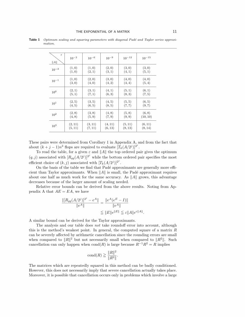
Table 1 Optimum scaling and squaring parameters with diagonal Pade and Taylor series approxi-mation.
ε
10−3 10−6 10−9 10−12 10−15
‖A‖
10−2 (1, 0)(1, 0)
(1, 0)(2, 1)
(2, 0)(3, 1)
(3, 0)(4, 1)
(3, 0)(5, 1)
10−1 (1, 0)(3, 0)
(2, 0)(4, 0)
(3, 0)(4, 2)
(4, 0)(4, 4)
(4, 0)(5, 4)
100 (2, 1)(5, 1)
(3, 1)(7, 1)
(4, 1)(6, 3)
(5, 1)(8, 3)
(6, 1)(7, 5)
101 (2, 5)(4, 5)
(3, 5)(6, 5)
(4, 5)(8, 5)
(5, 5)(7, 7)
(6, 5)(9, 7)
102 (2, 8)(4, 8)
(3, 8)(5, 9)
(4, 8)(7, 9)
(5, 8)(9, 9)
(6, 8)(10, 10)
103 (2, 11)(5, 11)
(3, 11)(7, 11)
(4, 11)(6, 13)
(5, 11)(8, 13)
(6, 11)(8, 14)
These pairs were determined from Corollary 1 in Appendix A, and from the fact thatabout (k + j − 1)n3 flops are required to evaluate [Tk(A/2j)]2
j
.To read the table, for a given ε and ‖A‖ the top ordered pair gives the optimum
(q, j) associated with [Rqq(A/2j)]2j
while the bottom ordered pair specifies the mostefficient choice of (k, j) associated with [Tk(A/2j)]2
j
.On the basis of the table we find that Pade approximants are generally more effi-
cient than Taylor approximants. When ‖A‖ is small, the Pade approximant requiresabout one half as much work for the same accuracy. As ‖A‖ grows, this advantagedecreases because of the larger amount of scaling needed.
Relative error bounds can be derived from the above results. Noting from Ap-pendix A that AE = EA, we have
‖[Rqq(A/2j)]2j − eA‖
‖eA‖ =‖eA(eE − I)‖
‖eA‖5 ‖E‖e‖E‖ 5 ε‖A‖eε‖A‖.
A similar bound can be derived for the Taylor approximants.The analysis and our table does not take roundoff error into account, although
this is the method’s weakest point. In general, the computed square of a matrix Rcan be severely affected by arithmetic cancellation since the rounding errors are smallwhen compared to ‖R‖2 but not necessarily small when compared to ‖R2‖. Suchcancellation can only happen when cond(R) is large because R−1R2 = R implies
cond(R) = ‖R‖2‖R2‖ .
The matrices which are repeatedly squared in this method can be badly conditioned.However, this does not necessarily imply that severe cancellation actually takes place.Moreover, it is possible that cancellation occurs only in problems which involve a large

12 CLEVE MOLER AND CHARLES VAN LOAN
hump. We regard it as an open question to analyze the roundoff error of the repeatedsquaring of eA/m and to relate the analysis to a realistic assessment of the sensitivityof eA.
In his implementation of scaling and squaring Ward [72] is aware of the possibilityof cancellation. He computes an a posteriori bound for the error, including the effectsof both truncation and roundoff. This is certainly preferable to no error estimate atall, but it is not completely satisfactory. A large error estimate could be the result ofany of three distinct difficulties:
(i) The error estimate is a severe overestimate of the true error, which is actuallysmall. The algorithm is stable but the estimate is too pessimistic.
(ii) The true error is large because of cancellation in going over the hump, but theproblem is not sensitive. The algorithm is unstable and another algorithmmight produce a more accurate answer.
(iii) The underlying problem is inherently sensitive. No algorithm can be expectedto produce a more accurate result.
Unfortunately, it is currently very difficult to distinguish among these three situations.Method 4. Chebyshev rational approximation. Let cqq(x) be the ratio of
two polynomials each of degree q and consider max05x<∞ |cqq(x)− e−x|. For variousvalues of q, Cody, Meinardus, and Varga [62] have determined the coefficients of theparticular cqq which minimizes this maximum. Their results can be directly translatedinto bounds for ‖cqq(A)− eA‖ when A is Hermitian with eigenvalues on the negativereal axis. The authors are interested in such matrices because of an application topartial differential equations. Their approach is particularly effective for the sparsematrices which occur in such applications.
For non-Hermitian (non-normal) A, it is hard to determine how well cqq(A) ap-proximates eA. If A has an eigenvalue λ off the negative real axis, it is possible forcqq(λ) to be a poor approximation to eλ. This would imply that cqq(A) is a poorapproximation to eA since
‖eA − cqq(A)‖ = |eλ − cqq(λ)|.
These remarks prompt us to emphasize an important facet about approxima-tion of the matrix exponential, namely, there is more to approximating eA than justapproximating ez at the eigenvalues of A. It is easy to illustrate this with Padeapproximation. Suppose
A =
0 6 0 00 0 6 00 0 0 60 0 0 0
.
Since all of the eigenvalues of A are zero, R11(z) is a perfect approximation to ez atthe eigenvalues. However,
R11(A) =
1 6 18 540 1 6 180 0 1 60 0 0 1
,

THE EXPONENTIAL OF A MATRIX 13
whereas
eA =
1 6 18 360 1 6 180 0 1 60 0 0 1
and thus,
‖eA −R11(A)‖ = 18.
These discrepancies arise from the fact that A is not normal. The example illustratesthat non-normality exerts a subtle influence upon the methods of this section eventhough the eigensystem, per se, is not explicitly involved in any of the algorithms.
4. Ordinary Differential Equation Methods. Since etA and etAx0 are solutionsto ordinary differential equations, it is natural to consider methods based on numeri-cal integration. Very sophisticated and powerful methods for the numerical solutionof general nonlinear differential equations have been developed in recent years. Allworthwhile codes have automatic step size control and some of them automaticallyvary the order of approximation as well. Methods based on single step formulas, mul-tistep formulas, and implicit multistep formulas each have certain advantages. Whenused to compute etA all these methods are easy to use and they require very littleadditional programming or other thought. The primary disadvantage is a relativelyhigh cost in computer time.
The o.d.e. programs are designed to solve a single system
x = f(x, t), x(0) = x0,
and to obtain the solution at many values of t. With f(x, t) = Ax the kth columnof etA can be obtained by setting x0 to the kth column of the identity matrix. Allthe methods involve a sequence of values 0 = t0, t1, · · · , tj = t with either fixed orvariable step size hi = ti+1− ti. They all produce vectors xi which approximate x(ti).
Method 5. General purpose o.d.e. solver. Most computer center librariescontain programs for solving initial value problems in ordinary differential equations.Very few libraries contain programs that compute etA. Until the latter programs aremore readily available, undoubtedly the easiest and, from the programmer’s point ofview, the quickest way to compute a matrix exponential is to call upon a general pur-pose o.d.e. solver. This is obviously an expensive luxury since the o.d.e. routine doesnot take advantage of the linear, constant coefficient nature of our special problem.
We have run a very small experiment in which we have used three recently devel-oped o.d.e. solvers to compute the exponentials of about a dozen matrices and havemeasured the amount of work required. The programs are:
(1) RKF45. Written by Shampine and Watts [108], this program uses the Fehlbergformulas of the Runge–Kutta type. Six function evaluations are required per step.The resulting formula is fifth order with automatic step size control. (See also [4].)
(2) DE/STEP. Written by Shampine and Gordon [107], this program uses variableorder, variable step Adams predictor-corrector formulas. Two function evaluations arerequired per step.
(3) IMPSUB. Written by Starner [109], this program is a modification of Gear’sDIFSUB [106] and is based on implicit backward differentiation formulas intended forstiff differential equations. Starner’s modifications add the ability to solve “infinitely

14 CLEVE MOLER AND CHARLES VAN LOAN
Table 2 Work as a function of subroutine and local error tolerance.
10−6 10−9 10−12
RKF45 217 832 3268
DE/STEP 118 160 211
IMPSUB 173 202 1510
stiff” problems in which the derivatives of some of the variables may be missing. Twofunction evaluations are usually required per step but three or four may occasionallybe used.
For RKF45 the output points are primarily determined by the step size selectionin the program. For the other two routines, the output is produced at user specifiedpoints by interpolation. For an n-by-n matrix A, the cost of one function evaluationis a matrix-vector multiplication or n2 flops. The number of evaluations is determinedby the length of the integration interval and the accuracy requested.
The relative performance of the three programs depends fairly strongly on theparticular matrix. RKF45 often requires the most function evaluations, especiallywhen high accuracy is sought, because its order is fixed. But it may well requirethe least actual computer time at modest accuracies because of its low overhead.DE/STEP indicates when it thinks a problem is stiff. If it doesn’t give this indication,it usually requires the fewest function evaluations. If it does, IMPSUB may requirefewer.
Table 2 gives the results for one particular matrix when we arbitrarily declare tobe a “typical” nonstiff problem. The matrix is of order 3, with eigenvalues λ = 3, 3, 6;the matrix is defective. We used three different local error tolerances and integratedover [0, 1]. The average number of function evaluations for the three starting vectorsis given in the table. These can be regarded as typical coefficients of n2 for the singlevector problem or of n3 for the full matrix exponential; IBM 370 long arithmetic wasused.
Although people concerned with the competition between various o.d.e. solversmight be interested in the details of this table, we caution that it is the result ofonly one experiment. Our main reason for presenting it is to support our contentionthat the use of any such routine must be regarded as very inefficient. The scalingand squaring method of section 3 and some of the matrix decomposition methods ofsection 6 require on the order of 10 to 20 n3 flops and they obtain higher accuraciesthan those obtained with 200 n3 or more flops for the o.d.e. solvers.
This excessive cost is due to the fact that the programs are not taking advantageof the linear, constant coefficient nature of the differential equation. They mustrepeatedly call for the multiplication of various vectors by the matrix A because, asfar as they know, the matrix may have changed since the last multiplication.
We now consider the various methods which result from specializing general o.d.e.methods to handle our specific problem.
Method 6. Single step o.d.e. methods. Two of the classical techniques forthe solution of differential equations are the fourth order Taylor and Runge–Kutta
THE EXPONENTIAL OF A MATRIX 15
methods with fixed step size. For our particular equation they become
xj+1 =(
I + hA + · · ·+ h4
4!A4
)xj = T4(hA)xj
and
xj+1 = xj + 16k1 + 1
3k2 + 13k3 + 1
6k4,
where k1 = hAxj , k2 = hA(xj + 12k1), k3 = hA(xj + 1
2k2), and k4 = hA(xj + k3). Alittle manipulation reveals that in this case, the two methods would produce identicalresults were it not for roundoff error. As long as the step size is fixed, the matrixT4(hA) need be computed just once and then xj+1 can be obtained from xj with justone matrix-vector multiplication. The standard Runge–Kutta method would require4 such multiplications per step.
Let us consider x(t) for one particular value of t, say t = 1. If h = 1/m, then
x(1) = x(mh) ' xm = [T4(hA)]mx0.
Consequently, there is a close connection between this method and Method 3 whichinvolved scaling and squaring [54], [60]. The scaled matrix is hA and its exponentialis approximated by T4(hA). However, even if m is a power of 2, [T4(hA)]m is usuallynot obtained by repeated squaring. The methods have roughly the same roundofferror properties and so there seem to be no important advantages for Runge–Kuttawith fixed step size.
Let us now consider the possibility of varying the step size. A simple algorithmmight be based on a variable step Taylor method. In such a method, two approxi-mations to xj+1 would be computed and their difference used to choose the step size.Specifically, let ε be some prescribed local relative error tolerance and define xj+1 andx∗j+1 by
xj+1 = T5(hjA)xj ,
x∗j+1 = T4(hjA)xj .
One way of determining hj is to require
‖xj+1 − x∗j+1‖ ' ε‖xj‖.
Notice that we are using a 5th order formula to compute the approximation, and a4th order formula to control step size.
At first glance, this method appears to be considerably less efficient than one withfixed step size because the matrices T4(hjA) and T5(hjA) cannot be precomputed.Each step requires 5 n2 flops. However, in those problems which involve large “humps”as described in section 1, a smaller step is needed at the beginning of the computationthan at the end. If the step size changes by a factor of more than 5, the variable stepmethod will require less work.
The method does provide some insight into the costs of more sophisticated inte-grators. Since
xj+1 − x∗j+1 =h5
jA5
5!xj ,
16 CLEVE MOLER AND CHARLES VAN LOAN
we see that the required step size is given approximately by
hj '[
5!ε‖A5‖
]1/5
.
The work required to integrate over some fixed interval is proportional to the inverseof the average step size. So, if we decrease the tolerance ε from, say 10−6 to 10−9,then the work is increased by a factor of (103)1/5 which is about 4. This is typical ofany 5th order error estimate—asking for 3 more figures roughly quadruples the work.
Method 7. Multistep o.d.e. solver. As far as we know, the possibilityof specializing multistep methods, such as those based on the Adams formulas, tolinear, constant coefficient problems has not been explored in detail. Such a methodwould not be equivalent to scaling and squaring because the approximate solution ata given time is defined in terms of approximate solutions at several previous times.The actual algorithm would depend upon how the starting vectors are obtained, andhow the step size and order are determined. It is conceivable that such an algorithmmight be effective, particularly for problems which involve a single vector, output atmany values of t, large n, and a hump.
The problems associated with roundoff error have not been of as much concernto designers of differential equation solvers as they have been to designers of matrixalgebra algorithms since the accuracy requested of o.d.e. solvers is typically less thanfull machine precision. We do not know what effect rounding errors would have in aproblem with a large hump.
5. Polynomial Methods. Let the characteristic polynomial of A be
c(z) = det(zI −A) = zn −n−1∑
k=0
ckzk.
From the Cayley–Hamilton theorem c(A) = 0 and hence
An = c0I + c1A + · · ·+ cn−1An−1.
It follows that any power of A can be expressed in terms of I, A, · · · , An−1:
Ak =n−1∑
j=0
βkjAj .
This implies that etA is a polynomial in A with analytic coefficients in t:
etA =∞∑
k=0
tkAk
k!=
∞∑
k=0
tk
k!
n−1∑
j=0
βkjAj
=n−1∑
j=0
[ ∞∑
k=0
βkjtk
k!
]Aj
≡n−1∑
j=0
αj(t)Aj .
The methods of this section involve this kind of exploitation of the characteristicpolynomial.

THE EXPONENTIAL OF A MATRIX 17
Method 8. Cayley–Hamilton. Once the characteristic polynomial is known,the coefficient βkj which define the analytic functions αj(t) =
∑βkjt
k/k! can begenerated as follows:
βkj =
δkj (k < n)cj (k = n)c0βk−1,n−1 (k > n, j = 0)cjβk−1,n−1 + βk−1,j−1 (k > n, j > 0).
One difficulty is that these recursive formulas for the βkj are very prone to roundofferror. This can be seen in the 1-by-1 case. If A = (α) then βk0 = αk and α0(t) =∑
(αt)k/k! is simply the Taylor series for eαt. Thus, our criticisms of Method 1 apply.In fact, if αt = −6, no partial sum of the series for eαt will have any significant digitswhen IBM 370 short arithmetic is used.
Another difficulty is the requirement that the characteristic polynomial must beknown. If λ1, · · · , λn are the eigenvalues of A, then c(z) could be computed fromc(z) =
∏n1 (z − λi). Although the eigenvalues could be stably computed, it is unclear
whether the resulting cj would be acceptable. Other methods for computing c(z) arediscussed in Wilkinson [14]. It turns out that methods based upon repeated powers ofA and methods based upon formulas for the cj in terms of various symmetric functionsare unstable in the presence of roundoff error and expensive to implement. Techniquesbased upon similarity transformations break down when A is nearly derogatory. Weshall have more to say about these difficulties in connection with Methods 12 and 13.
In Method 8 we attempted to expand etA in terms of the matrices I, A, · · · , An−1.If {A0, · · · , An−1} is some other set of matrices which span the same subspace, thenthere exist analytic functions βj(t) such that
etA =n−1∑
j=0
βj(t)Aj .
The convenience of this formula depends upon how easily the Aj and βj(t) can begenerated. If the eigenvalues λ1, · · · , λn of A are known, we have the following threemethods.
Method 9. Lagrange interpolation.
etA =n−1∑
j=0
eλjtn∏
k=1k 6=j
(A− λkI)(λj − λk)
.
Method 10. Newton interpolation.
etA = eλ1tI +n∑
j=2
[λ1, · · · , λj ]j−1∏
k=1
(A− λkI).
The divided differences [λ1, · · · , λj ] depend on t and are defined recursively by
[λ1, λ2] = (eλ1t − eλ2t)/(λ1 − λ2),
[λ1, · · · , λk+1] =[λ1, · · · , λk]− [λ2, · · · , λk+1]
λ1 − λk+1(k = 2).

18 CLEVE MOLER AND CHARLES VAN LOAN
We refer to MacDuffee [9] for a discussion of these formulae in the confluent eigenvaluecase.
Method 11. Vandermonde. There are other methods for computing thematrices
Aj =n∏
k=1k 6=j
(A− λkI)(λj − λk)
which were required in Method 9. One of these involves the Vandermonde matrix
V =
1 1 · · · 1λ1 λ2 · · · λn...
......
λn−11 λn−1
2 · · · λn−1n
.
If νjk is the (j, k) entry of V −1, then
Aj =n∑
k=1
νjkAk−1,
and
etA =n∑
j=1
eλjtAj .
When A has repeated eigenvalues, the appropriate confluent Vandermonde matrix isinvolved. Closed expressions for the νjk are available and Vidysager [92] has proposedtheir use.
Methods 9, 10, and 11 suffer on several accounts. They are O(n4) algorithmsmaking them prohibitively expensive except for small n. If the spanning matricesA0, · · · , An−1 are saved, then storage is n3 which is an order of magnitude greaterthan the amount of storage required by any “nonpolynomial” method. Furthermore,even though the formulas which define Methods 9, 10, and 11 have special form inthe confluent case, we do not have a satisfactory situation. The “gray” area of nearconfluence poses difficult problems which are best discussed in the next section ondecomposition techniques.
The next two methods of this section do not require the eigenvalues of A andthus appear to be free of the problems associated with confluence. However, equallyformidable difficulties attend these algorithms.
Method 12. Inverse Laplace transforms. If L[etA] is the Laplace trans-form of the matrix exponential, then
L[etA] = (sI −A)−1.
The entries of this matrix are rational functions of s. In fact,
(sI −A)−1 =n−1∑
k=0
sn−k−1
c(s)Ak,
where c(s) = det(sI −A) = sn −∑n−1k=0 cksk and for k = 1, · · · , n:
cn−k = −trace(Ak−1A)/k, Ak = Ak−1A− cn−kI (A0 = I).

THE EXPONENTIAL OF A MATRIX 19
These recursions were derived by Leverrier and Faddeeva [3] and can be used toevaluate etA:
etA =n−1∑
k=0
L−1[sn−k−1/c(s)]Ak,
The inverse transforms L−1[sn−k−1/c(s)] can be expressed as a power series in t. Liou[102] suggests evaluating these series using various recursions involving the ck. Wesuppress the details of this procedure because of its similarity to Method 8. There areother ways Laplace transforms can be used to evaluate etA [78], [80], [88], [89], [93].By and large, these techniques have the same drawbacks as Methods 8–11. They areO(n4) for general matrices and may be seriously effected by roundoff error.
Method 13. Companion matrix. We now discuss techniques which involvethe computation of eC where C is a companion matrix:
C =
0 1 0 · · · 00 0 1 · · · 0...
......1
c0 c1 c2 · · · cn−1
.
Companion matrices have some interesting properties which various authors have triedto exploit:
(i) C is sparse.(ii) The characteristic polynomial of C is c(z) = zn −∑n−1
k=0 ckzk.(iii) If V is the Vandermonde matrix of eigenvalues of C (see Method 11), then
V −1CV is in Jordan form. (Confluent Vandermonde matrices are involved in themultiple eigenvalue case.)
(iv) If A is not derogatory, then it is similar to a companion matrix; otherwiseit is similar to a direct sum of companion matrices.
Because C is sparse, small powers of C cost considerably less than the usual n3
flops. Consequently, one could implement Method 3 (scaling and squaring) with areduced amount of work.
Since the characteristic polynomial of C is known, one can apply Method 8 orvarious other techniques which involve recursions with the ck. However, this is notgenerally advisable in view of the catastrophic cancellation that can occur.
As we mentioned during our discussion of Method 11, the closed expression forV −1 is extremely sensitive. Because V −1 is so poorly conditioned, exploitation ofproperty (iii) will generally yield a poor estimate of eA.
If A = Y CY −1, then from the series definition of the matrix exponential it is easyto verify that
eA = Y eCY −1.
Hence, property (iv) leads us to an algorithm for computing the exponential of ageneral matrix. Although the reduction of A to companion form is a rational process,the algorithm for accomplishing this are extremely unstable and should be avoided[14].
We mention that if the original differential equation is actually a single nth orderequation written as a system of first order equations, then the matrix is already in

20 CLEVE MOLER AND CHARLES VAN LOAN
companion form. Consequently, the unstable reduction is not necessary. This is theonly situation in which companion matrix methods should be considered.
We conclude this section with an interesting aside on computing eH where H =(hij) is lower Hessenberg (hij = 0, j > i + 1). Notice that companion matrices arelower Hessenberg. Our interest in computing eH stems from the fact that any realmatrix A is orthogonally similar to a lower Hessenberg matrix. Hence, if
A = QHQT , QT Q = I,
then
eA = QeHQT .
Unlike the reduction to companion form, this factorization can be stably computedusing the EISPACK routine ORTHES [113].
Now, let fk denote the kth column of eH . It is easy to verify that
Hfk =n∑
i=k−1
hikfi (k = 2),
by equating the kth columns in the matrix identity HeH = eHH. If none of thesuperdiagonal entries hk−1,k are zero, then once fn is known, the other fk followimmediately from
fk−1 =1
hk−1,k
[Hfk −
n∑
i=k
hikfi
].
Similar recursive procedures have been suggested in connection with computing eC
[104]. Since fn equals x(1) where x(t) solves Hx = x, x(0) = (0, · · · , 0, 1)T , it couldbe found using one of the o.d.e. methods in the previous section.
There are ways to recover in the above algorithm should any of the hk−1,k be zero.However, numerically the problem is when we have a small, but non-negligible hk−1,k.In this case rounding errors involving a factor of 1/hk−1,k will occur precluding thepossibility of an accurate computation of eH .
In summary, methods for computing eA which involve the reduction of A tocompanion or Hessenberg form are not attractive. However, there are other matrixfactorizations which can be more satisfactorily exploited in the course of evaluatingeA and these will be discussed in the next section.
6. Matrix Decomposition Methods. The methods which are likely to be mostefficient for problems involving large matrices and repeated evaluation of etA are thosewhich are based on factorizations or decompositions of the matrix A. If A happensto be symmetric, then all these methods reduce to a simple very effective algorithm.
All the matrix decompositions are based on similarity transformations of the form
A = SBS−1.
As we have mentioned, the power series definition of etA implies
etA = SetBS−1.
The idea is to find an S for which etB is easy to compute. The difficulty is that Smay be close to singular which means that cond(S) is large.

THE EXPONENTIAL OF A MATRIX 21
Method 14. Eigenvectors. The naive approach is to take S to be the matrixwhose columns are eigenvectors of A, that is, S = V where
V = [v1| · · · |vn]
and
Avj = λjvj , j = 1, · · · , n.
These n equations can be written
AV = V D.
where D = diag(λ1, · · · , λn). The exponential of D is trivial to compute assuming wehave a satisfactory method for computing the exponential of a scalar:
etD = diag(eλ1t, · · · , eλnt).
Since V is nonsingular we have etA = V etDV −1.In terms of the differential equation x = Ax, the same eigenvector approach takes
the following form. The initial condition is a combination of the eigenvectors,
x(0) =n∑
j=1
αjvj ,
and the solution x(t) is given by
x(t) =n∑
j=0
αjeλjtvj .
Of course, the coefficients αj are obtained by solving a set of linear equations V α =x(0).
The difficulty with this approach is not confluent eigenvalues per se. For example,the method works very well when A is the identity matrix, which has an eigenvalueof the highest possible multiplicity. It also works well for any other symmetric matrixbecause the eigenvectors can be chosen orthogonal. If reliable subroutines such asTRED2 and TQL2 in EISPACK [113] are used, then the computed vj will be orthog-onal to the full accuracy of the computer and the resulting algorithm for etA has allthe attributes we desire—except that it is limited to symmetric matrices.
The theoretical difficulty occurs when A does not have a complete set of linearlyindependent eigenvectors and is thus defective. In this case there is no invertiblematrix of eigenvectors V and the algorithm breaks down. An example of a defectivematrix is
[1 10 1
].
A defective matrix has confluent eigenvalues but a matrix which has confluent eigen-values need not be defective.
In practice, difficulties occur when A is “nearly” defective. One way to makethis precise is to use the condition number, cond(V ) = ‖V ‖‖V −1‖, of the matrixof eigenvectors. If A is nearly (exactly) defective, then cond(V ) is large (infinite).

22 CLEVE MOLER AND CHARLES VAN LOAN
Any errors in A, including roundoff errors in its computation and roundoff errorsfrom the eigenvalue computation, may be magnified in the final result by cond(V ).Consequently, when cond(V ) is large, the computed etA will most likely be inaccurate.For example, if
A =[1 + ε 1
0 1− ε
],
then
V =[1 −10 2ε
],
D = diag(1 + ε, 1− ε),
and
cond(V ) = O
(1ε
).
If ε = 10−5 and IBM 370 short floating point arithmetic is used to compute theexponential from the formula eA = V eDV −1, we obtain
[2.718307 2.750000
0 2.718254
].
Since the exact exponential to six decimals is[2.718309 2.718282
0 2.718255
],
we see that the computed exponential has errors of order 105 times the machineprecision as conjectured.
One might feel that for this example eA might be particularly sensitive to pertur-bations in A. However, when we apply Theorem 3 in section 2 to this example, wefind
‖e(A+E) − eA‖‖eA‖ 5 4‖E‖e2‖E‖,
independent of ε. Certainly, eA is not overly sensitive to changes in A and so Method14 must be regarded as unstable.
Before we proceed to the next method it is interesting to note the connectionbetween the use of eigenvectors and Method 9, Lagrange interpolation. When theeigenvalues are distinct the eigenvector approach can be expressed
etA = V diag(eλjt)V −1 =n∑
j=1
eλjtvjyTj ,
where yTj is the jth row of V −1. The Lagrange formula is
etA =n∑
j=1
eλjtAj ,

THE EXPONENTIAL OF A MATRIX 23
where
Aj =n∏
k=1k 6=j
(A− λkI)(λj − λk)
.
Because these two expressions hold for all t, the individual terms in the sum must bethe same and so
Aj = vjyTj .
This indicates that the Aj are, in fact, rank one matrices obtained from the eigen-vectors. Thus, the O(n4) work involved in the computation of the Aj is totallyunnecessary.
Method 15. Triangular systems of eigenvectors. An improvement inboth the efficiency and the reliability of the conventional eigenvector approach canbe obtained when the eigenvectors are computed by the QR algorithm [14]. Assumetemporarily that although A is not symmetric, all its eigenvalues happen to be real.The idea is to use EISPACK subroutines ORTHES and HQR2 to compute the eigen-values and eigenvectors [113]. These subroutines produce an orthogonal matrix Q anda triangular matrix T so that
QT AQ = T.
Since Q−1 = QT , this is a similarity transformation and the desired eigenvalues occuron the diagonal of T . HQR2 next attempts to find the eigenvectors of T . This resultsin a matrix R and a diagonal matrix D, which is simply the diagonal part of T , sothat
TR = RD.
Finally, the eigenvectors of A are obtained by a simple matrix multiplication V = QR.The key observation is that R is upper triangular. In other words, the
ORTHES/HQR2 path in ISPACK computes the matrix of eigenvectors by first com-puting its “QR” factorization. HQR2 can be easily modified to remove the final multi-plication of Q and R. The availability of these two matrices has two advantages. First,the time required to find V −1 or to solve systems involving V is reduced. However,since this is a small fraction of the total time required, the improvement in efficiencyis not very significant. A more important advantage is that cond(V ) = cond(R) (inthe 2-norm) and that the estimation of cond(R) can be done reliably and efficiently.
The effect of admitting complex eigenvalues is that R is not quite triangular, buthas 2-by-2 blocks on its diagonal for each complex conjugate pair. Such a matrix iscalled quasi-triangular and we avoid complex arithmetic with minor inconvenience.
In summary, we suspect the following algorithm to be reliable:(1) Given A, use ORTHES and a modified HQR2 to find orthogonal Q, diagonal
D, and quasi-triangular R so that
AQR = QRD.
(2) Given x0, compute y0 by solving
Ry0 = QT x0.
Also estimate cond(R) and hence the accuracy of y0.

24 CLEVE MOLER AND CHARLES VAN LOAN
(3) If cond(R) is too large, indicate that this algorithm cannot solve the problemand exit.
(4) Given t, compute x(t) by
x(t) = V etDy0.
(If we want to compute the full exponential, then in Step 2 we solve RY = QT forY and then use etA = V etDY in Step 4.) It is important to note that the first threesteps are independent of t, and that the fourth step, which requires relatively littlework, can be repeated for many values of t.
We know there are examples where the exit is taken in Step 3 even though theunderlying problem is not poorly conditioned implying that the algorithm is unstable.Nevertheless, the algorithm is reliable insofar as cond(R) enables us to assess theerrors in the computed solution when that solution is found. It would be interestingto code this algorithm and compare it with Ward’s scaling and squaring program forMethod 3. In addition to comparing timings, the crucial question would be how oftenthe exit in Step 3 is taken and how often Ward’s program returns an unacceptablylarge error bound.
Method 16. Jordan canonical form. In principle, the problem posed bydefective eigensystems can be solved by resorting to the Jordan canonical form (JCF).If
A = P [J1 ⊕ · · · ⊕ Jk]P−1
is the JCF of A, then
etA = P [etJ1 ⊕ · · · ⊕ etJk ]P−1.
The exponentials of the Jordan blocks Ji can be given in closed form. For example, if
Ji =
λi 1 0 00 λi 1 00 0 λi 10 0 0 λi
,
then
etJi = eλit
1 t t2/2! t3/3!
0 1 t t2/2!0 0 1 t0 0 0 1
.
The difficulty is that the JCF cannot be computed using floating point arithmetic.A single rounding error may cause some multiple eigenvalue to become distinct or viceversa altering the entire structure of J and P . A related fact is that there is no apriori bound on cond(P ). For further discussion of the difficulties of computing theJCF, see the papers by Golub and Wilkinson [110] and Kagstrom and Ruhe [111].
Method 17. Schur. The Schur decomposition
A = QTQT
with orthogonal Q and triangular T exists if A has real eigenvalues. If A has complexeigenvalues, then it is necessary to allow 2-by-2 blocks on the diagonal of T or to
THE EXPONENTIAL OF A MATRIX 25
make Q and T complex (and replace QT with Q∗). The Schur decomposition canbe computed reliably and quite efficiently by ORTHES and a short-ended version ofHQR2. The required modifications are discussed in the EISPACK guide [113].
Once the Schur decomposition is available,
etA = QetT QT .
The only delicate part is the computation of etT where T is a triangular or quasi-triangular matrix. Note that the eigenvectors of A are not required.
Computing functions or triangular matrices is the subject of a recent paper byParlett [112]. If T is upper triangular with diagonal elements λ1, · · · , λn, then it isclear that etT is upper triangular with diagonal elements eλ1t, · · · , eλnt. Parlett showshow to compute the off-diagonal elements of etT recursively from divided differencesof the eλit. The example in section 1 illustrates the 2-by-2 case.
Again, the difficulty is magnification of roundoff error caused by nearly confluenteigenvalues λi. As a step towards handling this problem, Parlett describes a general-ization of his algorithm applicable to block upper triangular matrices. The diagonalblocks are determined by clusters of nearby eigenvalues. The confluence problems donot disappear, but they are confined to the diagonal blocks where special techniquescan be applied.
Method 18. Block diagonal. All methods which involve decompositions ofthe form
A = SBS−1
involve two conflicting objectives:1. Make B close to diagonal so that etB is easy to compute.2. Make S well conditioned so that errors are not magnified.
The Jordan canonical form places all the emphasis on the first objective, while theSchur decomposition places most of the emphasis on the second. (We would regardthe decomposition with S = I and B = A as placing even more emphasis on thesecond objective.)
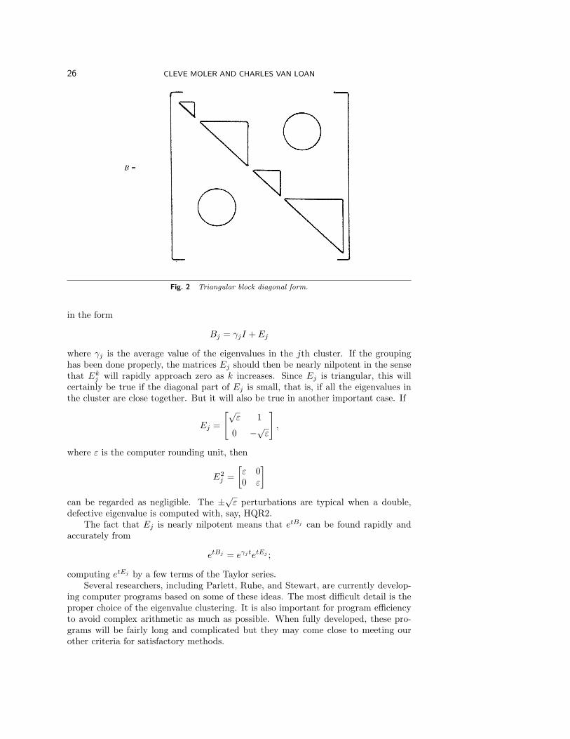
The block diagonal method is a compromise between these two extremes. Theidea is to use a nonorthogonal, but well conditioned, S to produce a B which istriangular and block diagonal as illustrated in Figure 2.
Each block in B involves a cluster of nearly confluent eigenvalues. The numberin each cluster (the size of each block) is to be made as small as possible whilemaintaining some prescribed upper bound for cond(S), such as cond(S) < 100. Thechoice of the bound 100 implies roughly that at most 2 significant decimal figures willbe lost because of rounding errors when etA is obtained from etB via etA = SetBS−1.A larger bound would mean the loss of more figures while a smaller bound wouldmean more computer time—both for the factorization itself and for the evaluation ofetB .
In practice, we would expect almost all the blocks to be 1-by-1 or 2-by-2 andthe resulting computation of etB to be very fast. The bound on cond(S) will meanthat it is occasionally necessary to have larger blocks in B, but it will insure againstexcessive loss of accuracy from confluent eigenvalues.
G. W. Stewart has pointed out that the grouping of the eigenvalues into clustersand the resulting block structure of B is not merely for increased speed. There canbe an important improvement in accuracy. Stewart suggests expressing each block Bj
26 CLEVE MOLER AND CHARLES VAN LOAN
Fig. 2 Triangular block diagonal form.
in the form
Bj = γjI + Ej
where γj is the average value of the eigenvalues in the jth cluster. If the groupinghas been done properly, the matrices Ej should then be nearly nilpotent in the sensethat Ek
j will rapidly approach zero as k increases. Since Ej is triangular, this willcertainly be true if the diagonal part of Ej is small, that is, if all the eigenvalues inthe cluster are close together. But it will also be true in another important case. If
Ej =
[√ε 1
0 −√ε
],
where ε is the computer rounding unit, then
E2j =
[ε 00 ε
]
can be regarded as negligible. The ±√ε perturbations are typical when a double,defective eigenvalue is computed with, say, HQR2.
The fact that Ej is nearly nilpotent means that etBj can be found rapidly andaccurately from
etBj = eγjtetEj ;
computing etEj by a few terms of the Taylor series.Several researchers, including Parlett, Ruhe, and Stewart, are currently develop-
ing computer programs based on some of these ideas. The most difficult detail is theproper choice of the eigenvalue clustering. It is also important for program efficiencyto avoid complex arithmetic as much as possible. When fully developed, these pro-grams will be fairly long and complicated but they may come close to meeting ourother criteria for satisfactory methods.

THE EXPONENTIAL OF A MATRIX 27
Most of the computational cost lies in obtaining the basic Schur decomposition.Although this cost varies somewhat from matrix to matrix because of the iterativenature of the QR algorithm, a good average figure is 15 n3 flops, including the furtherreduction to block diagonal form. Again we emphasize that the reduction is indepen-dent of t. Once the decomposition is obtained, the calculation of etA requires about 2n3 flops for each t. If we require only x(t) = etAx0 for various t, the equation Sy = x0
should be solved once at a cost of n3/3 flops, and then each x(t) can be obtained withn2 flops.
These are rough estimates. There will be differences between programs based onthe Schur decomposition and those which work with the block diagonal form, but thetimings should be similar because Parlett’s algorithm for the exponential is very fast.
7. Splitting Methods. A most aggravating, yet interesting, property of the ma-trix exponential is that the familiar additive law fails unless we have commutivity:
etBetC = et(B+C) ⇔ BC = CB.
Nevertheless, the exponentials of B and C are related to that of B + C, for example,by the Trotter product formula [30]:
eB+C = limm→∞
(eB/meC/m)m.
Method 19. Splitting. Our colleagues M. Gunzburger and D. Gottleib sug-gested that the Trotter result be used to approximate eA by splitting A into B + Cand then using the approximation
eA ' (eB/meC/m)m.
This approach to computing eA is of potential interest when the exponentials of Band C can be accurately and efficiently computed. For example, if B = (A + AT )/2and C = (A−AT )/2 then eB and eC can be effectively computed by the methods ofsection 5. For this choice we show in Appendix B that
(7.1) ‖eA − (eB/meC/m)m‖ 5 ‖[AT , A]‖4m
eµ(A),
where µ(A) is the log norm of A as defined in section 2. In the following algorithm,this inequality is used to determine the parameter m.
(a) Set B = (A + AT )/2 and C = (A − AT )/2. Compute the factorizationB = Q diag(µi)QT (QT Q = I) using TRED2 and TQL2 [113]. Variations ofthese programs can be used to compute the factorization C = UDUT whereUT U = I and D is the direct sum of zero matrices and real 2-by-2 blocks ofthe form
[0 a
−a 0
]
corresponding to eigenvalues ±ia.(b) Determine m = 2j such that the upper bound in (7.1) is less than some
prescribed tolerance. Recall that µ(A) is the most positive eigenvalue of Band that this quantity is known as a result of step (a).

28 CLEVE MOLER AND CHARLES VAN LOAN
(c) Compute X = Q diag(eµi/m)QT and Y = UeD/mUT . In the latter compu-tation, one uses the fact that
exp[
0 a/m
−a/m 0
]=
[cos(a/m) sin(a/m)
− sin(a/m) cos(a/m)
]
(d) Compute the approximation, (XY )2j
, to eA by repeated squaring.If we assume 5n3 flops for each of the eigenvalue decompositions in (a), then
the overall process outlined above requires about (13 + j)n3 flops. It is difficult toassess the relative efficiency of this splitting method because it depends strongly onthe scalars ‖[AT , A]‖ and µ(A) and these quantities have not arisen in connectionwith any of our previous eighteen methods. On the basis of truncation error bounds,however, it would seem that this technique would be much less efficient than Method3 (scaling and squaring) unless µ(A) were negative and ‖[AT , A]‖ much less than ‖A‖.
Accuracy depends on the rounding errors which arise in (d) as a result of therepeated squaring. The remarks about repeated squaring in Method 3 apply also here:there may be severe cancellation but whether or not this only occurs in sensitive eA
problems is unknown.For a general splitting A = B + C, we can determine m from the inequality
(7.2) ‖eA − (eB/meC/m)m‖ 5 ‖[B, C]‖2m
e‖B‖+‖C‖,
which we establish in Appendix B.To illustrate, suppose A has companion form
A =
0 1 0 · · · 0...
...1
c0 c1 · · · cn−1
.
If
B =
[0 In−1
0 0
]
and C = encT where cT = (c0, · · · , cn−1) and eTn = (0, 0, · · · , 0, 1), then
eB/m =n−1∑
k=0
[B
m
]k 1k!
and
eC/m = I +ecn−1/m − 1
cn−1encT .
Notice that the computation of these scaled exponentials require only O(n2) flops.Since ‖B‖ = 1, ‖C‖ = ‖c‖, and ‖[B, C]‖ 5 2‖c‖, (7.2) becomes
‖eA − (eB/meC/m)m‖ 5 e1+‖c‖‖c‖m
.
The parameter m can be determined from this inequality.
THE EXPONENTIAL OF A MATRIX 29
8. Conclusions. A section called “conclusions” must deal with the obvious ques-tion: Which method is best? Answering that question is very risky. We don’t knowenough about the sensitivity of the original problem, or about the detailed perfor-mance of careful implementations of various methods to make any firm conclusions.Furthermore, by the time this paper appears in the open literature, any given conclu-sion might well have to be modified.
We have considered five general classes of methods. What we have called poly-nomial methods are not really in the competition for “best”. Some of them requirethe characteristic polynomial and so are appropriate only for certain special problemsand others have the same stability difficulties as matrix decomposition methods butare much less efficient. The approaches we have outlined under splitting methods arelargely speculative and untried and probably only of interest in special settings. Thisleaves three classes in the running.
The only generally competitive series method is Method 3, scaling and squaring.Ward’s program implementing this method is certainly among the best currentlyavailable. The program may fail, but at least it tells you when it does. We don’tknow yet whether or not such failures usually result from the inherent sensitivity ofthe problem or from the instability of the algorithm. The method basically computeseA for a single matrix A. To compute etA for p arbitrary values of t requires aboutp times as much work. The amount of work is O(n3), even for the vector problemetAx0. The coefficient of n3 increases as ‖A‖ increases.
Specializations of o.d.e. methods for the eA problem have not yet been imple-mented. The best method would appear to involve a variable order, variable stepdifference scheme. We suspect it would be stable and reliable but expensive. Itsbest showing on efficiency would be for the vector problem etAx0 with many valuesof t since the amount of work is only O(n2). It would also work quite well for vec-tor problems involving a large sparse A since no “nonsparse” approximation to theexponential would be explicitly required.
The best programs using matrix decomposition methods are just now being writ-ten. They start with the Schur decomposition and include some sort of eigenvalueclustering. There are variants which involve further reduction to a block form. In allcases the initial decomposition costs O(n3) steps and is independent of t and ‖A‖. Af-ter that, the work involved in using the decomposition to compute etAx0 for differentt and x0 is only a small multiple of n2.
Thus, we see perhaps three or four candidates for “best” method. The choice willdepend upon the details of implementation and upon the particular problem beingsolved.
Appendix A. Inverse Error Analysis of Pade Matrix Approximation.Lemma 1. If ‖H‖ < 1, then log(I + H) exists and
‖ log(I + H)‖ 5 ‖H‖1− ‖H‖ .
Proof. If ‖H‖ < 1 then log(I + H) =∑∞
k=1(−1)k+1(Hk/k) and so
‖ log(I + H)‖ 5∞∑
k=1
‖H‖k
k5 ‖H‖
∞∑
k=0
‖H‖k =‖H‖
1− ‖H‖ .
Lemma 2. If ‖A‖ 5 12 and p > 0, then ‖Dpq(A)−1‖ 5 (q + p)/p.

30 CLEVE MOLER AND CHARLES VAN LOAN
Proof. From the definition of Dpq(A) in section 3, Dpq(A) = I + F where
F =q∑
j=1
(p + q − j)!q!(p + q)!(q − j)!
(−A)j
j!.
Using the fact that
(p + q − j)!q!(p + q)!(q − j)!
5[
q
p + q
]j
we find
‖F‖ 5q∑
j=1
[q
p + q‖A‖
]j 1j!
5 q
p + q‖A‖(e− 1) 5 q
p + q
and so ‖Dpq(A)−1‖ = ‖(I + F )−1‖ 5 1/(1− ‖F‖) 5 (q + p)/p.Lemma 3. If ‖A‖ 5 1
2 , q 5 p, and p = 1, then Rpq(A) = eA+F where
‖F‖ 5 8‖A‖p+q+1 p!q!(p + q)!(p + q + 1)!
.
Proof. From the remainder theorem for Pade approximants [71],
Rpq(A) = eA − (−1)q
(p + q)!Ap+q+1Dpq(A)−1
∫ 1
0
e(1−u)Aup(1− u)q du,
and so e−ARpq(A) = I + H where
H =(−1)q+1
(p + q)!Ap+q+1Dpq(A)−1
∫ 1
0
e−uAup(1− u)q du.
By taking norms, using Lemma 2, and noting that (p + q)/pe.5 5 4 we obtain
‖H‖ 5 1(p + q)!
‖A‖p+q+1 p + q
p
∫ 1
0
e.5up(1− u)q du
5 4‖A‖p+q+1 p!q!(p + q)!(p + q + 1)!
.
With the assumption ‖A‖ 5 12 it is possible to show that for all admissible p and q,
‖H‖ 5 12 and so from Lemma 1,
‖ log(I + H)‖ 5 ‖H‖1− ‖H‖ 5 8‖A‖p+q+1 p!q!
(p + q)!(p + q + 1)!.
Setting F = log(I + H), we see that e−ARpq(A) = I + H = eF . The lemma nowfollows because A and F commute implying Rpq(A) = eAeF = eA+F .
Lemma 4. If ‖A‖ 5 12 then Rpq(A) = eA+F where
‖F‖ 5 8‖A‖p+q+1 p!q!(p + q)!(p + q + 1)!
.
THE EXPONENTIAL OF A MATRIX 31
Proof. The case p = q, p = 1 is covered by Lemma 1. If p + q = 0, then F = −Aand the above inequality holds. Finally, consider the case q > p, q = 1. From Lemma3, Rqp(−A) = e−A+F where F satisfies the above bound. The lemma now followsbecause ‖ − F‖ = ‖F‖ and Rpq(A) = [Rqp(−A)]−1 = [e−A+F ]−1 = eA−F .
Theorem 4. If ‖A‖/2j 5 12 , then [Rpq(A/2j)]2
j
= eA+E where
‖E‖‖A‖ 5 8
(‖A‖2j
)p+qp!q!
(p + q)!(p + q + 1)!5
(12
)p+q−3p!q!
(p + q)!(p + q + 1)!.
Proof. From Lemma 4, Rpq(A/2j) = eA/2j+F where
‖F‖ 5 8[‖A‖
2j
]p+q+1p!q!
(p + q)!(p + q + 1)!.
The theorem follows by noting that if E = 2jF , then
[Rpq
(A
2j
)]2j
= [eA/2j+F ]2j
= eA+E .
Corollary 1. If ‖A‖/2j 5 12 , then [Tk(A/2j)]2
j
= eA+E where
‖E‖‖A‖ 5 8
(‖A‖2j
)k
· 1k + 1
5(
12
)k−3 1k + 1
.
Corollary 2. If ‖A‖/2j 5 12 , then [Rqq(A/2j)]2j = eA+E, where
‖E‖‖A‖ 5 8
(‖A‖2j
)2q
· (q!)2
(2q)!(2q + 1)!5
(12
)2q−3 (q!)2
(2q)!(2q + 1)!.
Appendix B. Accuracy of Splitting Techniques. In this appendix we derive theinequalities (7.1) and (7.2). We assume throughout that A is an n-by-n matrix andthat
A = B + C.
It is convenient to define the matrices
Sm = eA/m,
and
Tm = eB/meC/m,
where m is a positive integer. Our goal is to bound ‖Smm − Tm
m ‖. To this end we shallhave to exploit the following properties of the log norm µ(A) defined in section 2:
(i) ‖etA‖ 5 eµ(A)t (t = 0)(ii) µ(A) 5 ‖A‖(iii) µ(B + C) 5 µ(B) + ‖C‖.

32 CLEVE MOLER AND CHARLES VAN LOAN
These and other results concerning log norms are discussed in references [35]–[42].Lemma 5. If Θ = max{µ(A), µ(B) + µ(C)} then
‖Smm − Tm
m ‖ 5 meΘ(m−1)/m‖Sm − Tm‖.Proof. Following Reed and Simon [11] we have
Smm − Tm
m =m−1∑
k=0
Skm(Sm − Tm)Tm−1−k
m .
Using log norm property (i) it is easy to show that both ‖Sm‖ and ‖Tm‖ are boundedabove by eΘ/m and thus
‖Smm − Tm
m ‖ 5m−1∑
k=0
‖Sm‖k‖Sm − Tm‖‖Tm‖m−1−k
≤ ‖Sm − Tm‖m−1∑
k=0
eΘk/meΘ(m−1−k)/m,
from which the lemma immediately follows.In Lemmas 6 and 7 we shall make use of the notation
F (t)|t=t1t=t0
= F (t1)− F (t0),
where F (t) is a matrix whose entries are functions of t.Lemma 6.
Tm − Sm =∫ 1
0
etB/m
[e(1−t)A/m,
1m
C
]etC/m dt.
Proof. We have Tm − Sm = etB/me(1−t)A/metC/m|t=1t=0 and thus
Tm − Sm =∫ 1
0
{d
dt[etB/me(1−t)A/metC/m]
}dt.
The lemma follows since
d
dt[etB/me(1−t)A/metC/m] = etB/m
[e(1−t)A/m,
1m
C
]etC/m.
Lemma 7. If X and Y are matrices then
‖[eX , Y ]‖ 5 eµ(X)‖[X, Y ]‖.Proof. We have [eX , Y ] = etXY e(1−t)X |t=1
t=0 and thus
[eX , Y ] =∫ 1
0
{d
dt[etXY e(1−t)X ]
}dt.
Since d/dt[etXY e(1−t)X ] = etX [X, Y ]e(1−t)X we get
‖[eX , Y ]‖ 5∫ 1
0
‖etX‖‖[X, Y ]‖‖e(1−t)X‖ dt
5 ‖[X, Y ]‖∫ 1
0
eµ(X)teµ(X)(1−t) dt

THE EXPONENTIAL OF A MATRIX 33
from which the lemma immediately follows.Theorem 5. If Θ = max{µ(A), µ(B) + µ(C)}, then
‖Smm − Tm
m ‖ 5 12m
eΘ‖[B, C]‖.
Proof. If 0 5 t 5 1 then an application of Lemma 7 with X ≡ (1 − t)A/m andY ≡ C/m yields
‖[e(1−t)A/m, C/m]‖ 5 eµ(A)(1−t)/m‖[(1− t)A/m,C/m]‖
≤ eΘ(1−t)/m (1− t)m2
‖[B,C]‖.
By coupling this inequality with Lemma 6 we can bound ‖Tm − Sm‖:
‖Tm − Sm‖ 5∫ 1
0
‖etB/m‖‖[e(1−t)A/m, C/m]‖‖etC/m‖ dt
5∫ 1
0
eµ(B)t/meΘ(1−t)/m (1− t)m2
‖[B, C]‖eµ(C)t/m dt
5 12eΘ/m ‖[B, C]‖
m2.
The theorem follows by combining this result with Lemma 5.Corollary 3. If B = (A + A∗)/2 and C = (A−A∗)/2 then
‖Smm − Tm
m ‖ 5 14m
eµ(A)‖[A∗, A]‖.
Proof. Since µ(A) = µ(B) and µ(C) = 0, we can set Θ = µ(A). The corollary isestablished by noting that [B, C] = 1
2 [A∗, A].Corollary 4.
‖Smm − Tm
m ‖ 5 12m
eµ(B)+‖C‖‖[B, C]‖ 5 12m
e‖B‖+‖C‖‖[B, C]‖.
Proof. max{µ(A), µ(B) + µ(C)} 5 µ(B) + ‖C‖ 5 ‖B‖+ ‖C‖.Acknowledgments. We have greatly profited from the comments and suggestions
of so many people that it is impossible to mention them all. However, we are partic-ularly obliged to B. N. Parlett and G. W. Stewart for their very perceptive remarksand to G. H. Golub for encouraging us to write this paper. We are obliged to Pro-fessor Paul Federbush of the University of Michigan for helping us with the analysisin Appendix B. Finally, we would like to thank the referees for their numerous andmost helpful comments.
REFERENCES
Background.[1] R. Bellman, Introduction to Matrix Analysis, McGraw-Hill, New York, 1969.[2] C. Davis, Explicit functional calculus, J. Linear Algebra Appl., 6 (1973), pp. 193–199.[3] V. N. Faddeeva, Computational Methods of Linear Algebra, Dover, New York, 1959.[4] G. E. Forsythe, M. A. Malcolm and C. B. Moler, Computer Methods for Mathematical
Computations, Prentice-Hall, Englewood Cliffs, NJ, 1977.

34 CLEVE MOLER AND CHARLES VAN LOAN
[5] J. S. Frame, Matrix functions and applications, Part II: Functions of matrices, IEEE Spec-trum, 1 (April, 1964), pp. 102–108.
[6] J. S. Frame, Matrix functions and applications, Part IV: Matrix functions and constituentmatrices, IEEE Spectrum, 1 (June, 1964), pp. 123–131.
[7] J. S. Frame, Matrix functions and applications, Part V: Similarity reductions by rational ororthogonal matrices, IEEE Spectrum, 1 (July, 1964), pp. 103–116.
[8] F. R. Gantmacher, The Theory of Matrices, Vols. I and II, Chelsea Publishing Co., NewYork, 1959.
[9] C. C. MacDuffee, The Theory of Matrices, Chelsea, New York, 1956.[10] L. Mirsky, An Introduction to Linear Algebra, Oxford University Press, London, 1955.[11] M. Reed and B. Simon, Functional Analysis, Academic Press, New York, 1972.[12] R. F. Rinehart, The equivalence of definitions of a matrix function, Amer. Math. Monthly,
62 (1955), pp. 395–414.[13] P. C. Rosenbloom, Bounds on functions of matrices, Amer. Math. Monthly, 74 (1967),
pp. 920–926.[14] J. H. Wilkinson, The Algebraic Eigenvalue Problem, Oxford University Press, Oxford, 1965.
Properties and representations.[15] T. M. Apostol, Some explicit formulas for the matrix exponential, Amer. Math. Monthly,
76 (1969), pp. 284–292.[16] R. W. Atherton and A. E. De Gance, On the evaluation of the derivative of the matrix
exponential function, IEEE Trans. Automatic Control, AC-20 (1975), pp. 707–708.[17] A. Bradshaw, The eigenstructure of sample data systems with confluent eigenvalues, Inter-
nat. J. Systems Sci., 5 (1975), pp. 607–613.[18] R. Bellman, Perturbation Techniques in Mathematics, Physics, and Engineering, Holt, Rine-
hart, and Winston, New York, 1964.[19] J. C. Cavendish, On the norm of a matrix exponential, SIAM Rev., 17 (1975), pp. 174–175.[20] C. G. Cullen, Remarks on computing eAt, IEEE Trans. Automatic Control, AC-16 (1971),
pp. 94–95.[21] F. Fer, Resolution de l’equation matricelle dU/dt = pU par produit infini d’exponentielles,
Acad. Roy. Belg. Bull. Cl. Sci., 44 (1958), pp. 819–829.[22] E. P. Fulmer, Computation of the matrix exponential, Amer. Math. Monthly, 82 (1975),
pp. 156–159.[23] B. Kagstrom, Bounds and perturbation bounds for the matrix exponential, BIT, 17 (1977),
pp. 39–57.[24] T. Kato, Perturbation Theory for Linear Operators, Chap. 9, Springer-Verlag, New York,
1966.[25] R. B. Kirchner, An explicit formula for eAt, Amer. Math. Monthly, 74 (1967), pp. 1200–
1204.[26] H. O. Kreiss, Uber Matrizen die beschrankte Halbgruppen erzeuge, Math. Scand., 7 (1959),
pp. 71–80.[27] D. L. Powers, On the eigenstructure of the matrix exponential, Internat. J. Systems Sci., 7
(1976), pp. 723–725.[28] E. J. Putzer, Avoiding the Jordan canonical form in the discussion of linear systems with
constant coefficients, Amer. Math. Monthly, 73 (1966), pp. 2–7.[29] N. M. Rice, More explicit formulas for the exponential matrix, Queen’s Mathematical
Reprints 1970–21, Queen’s University, Kingston, Ontario, 1970.[30] H. F. Trotter, Product of semigroups of operators, Proc. Amer. Math. Soc., 10 (1959),
pp. 545–551.[31] C. F. Van Loan, A study of the matrix exponential, Numerical Analysis Report 7, Department
of Mathematics, University of Manchester, Manchester, England, 1975.[32] C. F. Van Loan, The sensitivity of the matrix exponential, SIAM J. Numer. Anal., 14 (1977),
pp. 971–981.[33] G. H. Weiss and A. A. Maradudin, The Baker–Hausdorff formula and a problem in crystal
physics, J. Math. and Phys., 3 (1962), pp. 771–777.[34] A. D. Ziebur, On determining the structure of A by analyzing eAt, SIAM Rev., 12 (1970),
pp. 98–102.
Log norms and stability.[35] W. A. Coppel, Stability and Asymptotic Behavior of Differential Equations, D. C. Heath,
Boston, 1965.[36] G. Dahlquist, Stability and error bounds in the numerical integration of ordinary differential

THE EXPONENTIAL OF A MATRIX 35
equations, Transactions of the Royal Institute of Technology 130, Stockholm, Sweden,1959.
[37] C. A. Desoer and H. Haneda, The measure of a matrix as a tool to analyze computeralgorithms for circuit analysis, IEEE Trans. Circuit Theory, CT-19 (1972), pp. 480–486.
[38] E. Deutsch, On matrix norms and logarithmic norms, Numer. Math., 24 (1975), pp. 49–51.[39] C. V. Pao, Logarithmic derivatives of a square matrix, J. Linear Algebra Appl., 6 (1973),
pp. 159–164.[40] C. V. Pao, A further remark on the logarithmic derivatives of a square matrix, J. Linear
Algebra Appl., 7 (1973), pp. 275–278.[41] T. Strom, Minimization of norms and logarithmic norms by diagonal similarities, Comput-
ing, 10 (1972), pp. 1–9.[42] T. Strom, On logarithmic derivatives, SIAM J. Numer. Anal., 12 (1975), pp. 741–753.
Survey articles.[43] M. Healey, Study of methods of computing transition matrices, Proc. IEEE, 120 (1973),
pp. 905–912.[44] C. B. Moler, Difficulties in computing the exponential of a matrix, Proceedings of the
Second USA–Japan Computer Conference, A.F.I.P.S., Montvale, NJ, 1975, pp. 79–82.
Truncated Taylor series.[45] L. Y. Bahar and A. K. Sinha, Matrix exponential approach to dynamic response, Computers
and Structures, 5 (1975), pp. 159–165.[46] T. A. Bickart, Matrix exponential: Approximation by truncated power series, Proc. IEEE,
56 (1968), pp. 372–373.[47] G. J. Bierman, Power series evaluation of transition and covariance matrices, IEEE Trans.
Automatic Control, AC-17 (1972), pp. 228–231.[48] D. A. Calahan, Numerical solution of linear systems with widely separated time constants,
Proc. IEEE, 55 (1967), pp. 2016–2017.[49] K. C. Daly, Evaluating the matrix exponential, Electron. Lett., 8 (1972), p. 390.[50] W. Everling, On the evaluation of eAt by power series, Proc. IEEE, 55 (1967), p. 413.[51] D. A. Gall, The solution of linear constant coefficient ordinary differential equations with
APL, Comput. Methods Mechanics and Engrg., 1 (1972), pp. 189–196.[52] M. L. Liou, A novel method of evaluating transient response, Proc. IEEE, 54 (1966), pp. 20–
23.[53] J. B. Mankin and J. C. Hung, On roundoff errors in computation of transition matrices,
Reprints of the Joint Automatic Control Conference, pp. 60–64, University of Colorado,Boulder, CO, 1969.
[54] E. J. Mastascusa, A relation between Liou’s method and fourth order Runge–Kutta methodfor evaluation of transient response, Proc. IEEE, 57 (1969), pp. 803–804.
[55] J. B. Plant, On the computation of transient matrices for time invariant systems, Proc.IEEE, 56 (1968), pp. 1397–1398.
[56] M. M. Shah, On the evaluation of eAt, Cambridge Report CUED/B-Control TR8, Cambridge,England, 1971.
[57] M. M. Shah, Analysis of roundoff and truncation errors in the computation of transitionmatrices, Cambridge Report CUED/B-Control TR12, Cambridge, England, 1971.
[58] C. J. Standish, Truncated Taylor series approximation to the state transition matrix of acontinuous parameter Markov chain, J. Linear Algebra Appl., 12 (1975), pp. 179–183.
[59] D. E. Whitney, Propagated error bounds for numerical solution of transient response, Proc.IEEE, 54 (1966), pp. 1084–1085.
[60] D. E. Whitney, More similarities between Runge–Kutta and matrix exponential methods forevaluating transient response, Proc. IEEE, 57 (1969), pp. 2053–2054.
Rational approximation.[61] J. L. Blue and H. K. Gummel, Rational approximations to the matrix exponential for sys-
tems of stiff differential equations, J. Comput. Phys., 5 (1970), pp. 70–83.[62] W. J. Cody, G. Meinardus and R. S. Varga, Chebyshev rational approximation to exp(−x)
in [0, +∞] and applications to heat conduction problems, J. Approx. Theory, 2 (1969),pp. 50–65.
[63] W. Fair and Y. Luke, Pade approximations to the operator exponential, Numer. Math., 14(1970), pp. 379–382.
[64] S. P. Norsett, C-polynomials for rational approximation to the exponential function, Numer.Math., 25 (1975), pp. 39–56.

36 CLEVE MOLER AND CHARLES VAN LOAN
[65] E. B. Saff, On the degree of best rational approximation to the exponential function, J.Approx. Theory, 9 (1973), pp. 97–101.
[66] E. B. Saff and R. S. Varga, On the zeros and poles of Pade approximants to exp(z), Numer.Math., 25 (1975), pp. 1–14.
[67] R. E. Scraton, Comment on rational approximants to the matrix exponential, Electron.Lett., 7 (1971), pp. 260–261.
[68] J. L. Siemieniuch, Properties of certain rational approximations to e−z , BIT, 16 (1976),pp. 172–191.
[69] G. Siemieniuch and I. Gladwell, On time discretizations for linear time dependent par-tial differential equations, Numerical Analysis Report 5, Department of Mathematics,University of Manchester, England, 1974.
[70] D. M. Trujillo, The direct numerical integration of linear matrix differential equations usingPade approximations, Internat. J. Numer. Methods Engrg., 9 (1975), pp. 259–270.
[71] R. S. Varga, On higher order stable implicit methods for solving parabolic partial differentialequations, J. Math. Phys., 40 (1961), pp. 220–231.
[72] R. C. Ward, Numerical computation of the matrix exponential with accuracy estimate, SIAMJ. Numer. Anal., 14 (1977), pp. 600–610.
[73] A. Wragg and C. Davies, Evaluation of the matrix exponential, Electron. Lett., 9 (1973),pp. 525–526.
[74] A. Wragg and C. Davies, Computation of the exponential of a matrix I: Theoretical con-siderations, J. Inst. Math. Appl., 11 (1973), pp. 369–375.
[75] A. Wragg and C. Davies, Computation of the exponential of a matrix II: Practical consid-erations, J. Inst. Math. Appl., 15 (1975), pp. 273–278.
[76] V. Zakian, Rational approximants to the matrix exponential, Electron. Lett., 6 (1970),pp. 814–815.
[77] V. Zakian and R. E. Scraton, Comments on rational approximations to the matrixexponential, Electron. Lett., 7 (1971), pp. 260–262.
Polynomial methods.[78] G. J. Bierman, Finite series solutions for the transition matrix and covariance of a time-
invariant system, IEEE Trans. Automatic Control, AC-16 (1971), pp. 173–175.[79] J. A. Boehm and J. A. Thurman, An algorithm for generating constituent matrices, IEEE
Trans. Circuit Theory, CT-18 (1971), pp. 178–179.[80] C. F. Chen and R. R. Parker, Generalization of Heaviside’s expansion technique to transi-
tion matrix evaluation, IEEE Trans. Educ., E-9 (1966), pp. 209–212.[81] W. C. Davidon, Exponential Function of a 2-by-2 Matrix, Hewlett-Packard HP65 Library
Program.[82] S. Deards, On the evaluation of exp(tA), Matrix Tensor Quart., 23 (1973), pp. 141–142.[83] S. Ganapathy and R. S. Rao, Transient response evaluation from the state transition matrix,
Proc. IEEE, 57 (1969), pp. 347–349.[84] I. C. Goknar, On the evaluation of constituent matrices, Internat. J. Systems Sci., 5 (1974),
pp. 213–218.[85] I. I. Kolodner, On exp(tA) with A satisfying a polynomial, J. Math. Anal. Appl., 52 (1975),
pp. 514–524.[86] Y. L. Kuo and M. L. Liou, Comments on “A novel method of evaluating eAt in closed
form”, IEEE Trans. Automatic Control, AC-16 (1971), p. 521.[87] E. J. Mastascusa, A method of calculating eAt based on the Cayley–Hamilton theorem, Proc.
IEEE, 57 (1969), pp. 1328–1329.[88] K. R. Rao and N. Ahmed, Heaviside expansion of transition matrices, Proc. IEEE, 56 (1968),
pp. 884-886.[89] K. R. Rao and N. Ahmed, Evaluation of transition matrices, IEEE Trans. Automatic Con-
trol, AC-14 (1969), pp. 779–780.[90] B. Roy, A. K. Mandal, D. Roy Choudhury, A. K. Choudhury, On the evaluation of the
state transition matrix, Proc. IEEE, 57 (1969), pp. 234–235.[91] M. N. S. Swamy, On a formula for evaluating eAt when the eigenvalues are not necessarily
distinct, Matrix Tensor Quart., 23 (1972), pp. 67–72.[92] M. Vidysager, A novel method of evaluating eAt in closed form, IEEE Trans. Automatic
Control, AC-15 (1970), pp. 600–601.[93] V. Zakian, Solution of homogeneous ordinary linear differential equations by numerical
inversion of Laplace transforms, Electron. Lett., 7 (1971), pp. 546–548.
Companion matrix methods.
THE EXPONENTIAL OF A MATRIX 37
[94] A. K. Choudhury, et al., On the evaluation of eAt, Proc. IEEE, 56 (1968), pp. 1110–1111.[95] L. Falcidieno and A. Luvinson, A numerical approach to computing the companion matrix
exponential, CSELT technical report 4, 1975, pp. 69–71.[96] C. J. Harris, Evaluation of matrix polynomials in the state companion matrix of linear time
invariant systems, Internat. J. Systems Sci., 4 (1973), pp. 301–307.[97] D. W. Kammler, Numerical evaluation of exp(At) when A is a companion matrix, unpub-
lished manuscript, University of Southern Illinois, Carbondale, IL, 1976.[98] I. Kaufman, Evaluation of an analytical function of a companion matrix with distinct eigen-
values, Proc. IEEE, 57 (1969), pp. 1180–1181.[99] I. Kaufman, A note on the “Evaluation of an analytical function of a companion matrix with
distinct eigenvalues”, Proc. IEEE, 57 (1969), pp. 2083–2084.[100] I. Kaufman and P. H. Roe, On systems described by a companion matrix, IEEE Trans.
Automatic Control, AC-15 (1970), pp. 692–693.[101] I. Kaufman, H. Mann and J. Vlach, A fast procedure for the analysis of linear time invariant
networks, IEEE Trans. Circuit Theory, CT-18 (1971), pp. 739–741.[102] M. L. Liou, Evaluation of the transition matrix, Proc. IEEE, 55 (1967), pp. 228–229.[103] A. K. Mandal, et al., Numerical computation method for the evaluation of the transition
matrix, Proc. IEEE, 116 (1969), pp. 500–502.[104] W. E. Thomson, Evaluation of transient response, Proc. IEEE, 54 (1966), p. 1584.
Ordinary differential equations.[105] B. L. Ehle and J. D. Lawson, Generalized Runge–Kutta processes for stiff initial value
problems, J. Inst. Math. Appl., 16 (1975), pp. 11–21.[106] C. W. Gear, Numerical Initial Value Problems in Ordinary Differential Equations, Prentice-
Hall, Englewood Cliffs, NJ, 1971.[107] L. F. Shampine and M. K. Gordon, Computer Solution of Ordinary Differential Equations—
The Initial Value Problem, W. H. Freeman and Co., San Francisco, 1975.[108] L. F. Shampine and H. A. Watts, Practical solution of ordinary differential equations by
Runge–Kutta methods, Sandia Lab Report SAND 76-0585 Albuquerque, NM, 1976.[109] J. Starner, Numerical solution of implicit differential-algebraic equations, Ph. D. Thesis,
University of New Mexico, Albuquerque, NM, 1976.
Matrix decomposition methods.[110] G. H. Golub and J. H. Wilkinson, Ill-conditioned eigensystems and the computation of the
Jordan canonical form, SIAM Rev., 18 (1976), pp. 578–619.[111] B. Kagstrom and A. Ruhe, An algorithm for numerical computation of the Jordan normal
form of a complex matrix, Report UMINF 51.74, Department of Information Processing,University of Umea, Umea, Sweden, 1974. Subsequently published in ACM Trans. Math.Software, 6 (1980), pp. 398–419.
[112] B. N. Parlett, A recurrence among the elements of functions of triangular matrices, LinearAlgebra Appl., 14 (1976), pp. 117–121.
[113] B. T. Smith, J. M. Boyle, J. J. Dongarra, B. S. Garbow, Y. Ikebe, V. C. Klema, C. B.Moler, Matrix Eigensystem Routines: EISPACK Guide, 2nd ed., Lecture Notes inComput. Sci. 6, Springer-Verlag, New York, 1976.
Integrals involving eAt.[114] E. S. Armstrong and A. K. Caglayan, An algorithm for the weighting matrices in the
sampled-data optimal linear regulator problem, NASA Technical Note, TN D-8372, 1976.[115] J. Johnson and C. L. Phillips, An algorithm for the computation of the integral of the state
transition matrix, IEEE Trans. Automat. Control, AC-16 (1971), pp. 204–205.[116] C. Kallstrom, Computing exp(A) and
Rexp(As) ds, Report 7309, Division of Automatic
Control, Lund Institute of Technology, Lund, Sweden, 1973.[117] A. H. Levis, Some computational aspects of the matrix exponential, IEEE Trans. Automat.
Control, AC-14 (1969), pp. 410–411.[118] C. F. Van Loan, Computing integrals involving the matrix exponential, Cornell Computer
Science Report TR 76-270, 1976, Subsequently published in IEEE Trans. Auto. Cont.AC-23 (1978), pp. 395–404
Selected applications.[119] F. H. Branin, Computer methods of network analysis, Proc. IEEE, 55 (1967), pp. 1787–1801.[120] R. Brockett, Finite Dimensional Linear Systems, John Wiley, New York, 1970.[121] K. F. Hansen, B. V. Koen and W. W. Little, Stable numerical solutions of the reactor

38 CLEVE MOLER AND CHARLES VAN LOAN
kinetics equations, Nuclear Sci. Engrg., 22 (1965), pp. 51–59.[122] J. A. W. da Nobrega, A new solution of the point kinetics equations, Nuclear Sci. Engrg.,
46 (1971), pp. 366–375.
9. Update, twenty-five years later. Since the publication of Nineteen Waystwenty-five years ago, the field of matrix computations has matured in several im-portant directions:
• There is a greater appreciation for non-normality and related issues of condi-tioning.
• Krylov-type methods for large sparse problems have been developed that arevery effective.
• Many structure-exploiting variants of the basic algorithms have been devel-oped which work well in specific application areas.
• High-performance methods have been developed for computers that have aheirarchical memory and/or multiple processing units.
All these developments have affected the matrix exponential “business”, somemore than others. This brief account of the past twenty-five years is not the distillationof an exhaustive literature search. Instead, we have chosen to highlight just a fewresearch threads, especially those that complement and expand upon the key ideas inNineteen Ways. We trust that our very incomplete bibliography provides adequatepointers for the interested reader.
A good place to begin the discussion is with the scaling and squaring methodthat is based upon Pade approximation (Method 3). It continues to attract a lotof attention relative to the other methods presented in Nineteen Ways. Bochev andMarkov [124] discuss its execution using interval arithmetic while Arioli, Codenatti,and Fassino [123] offer analyses for several important structured examples.
While on the topic of Pade approximation and scaling and squaring it is interest-ing to note that analogous algorithmic techniques have been developed for the matrixlogarithm problem. See Cheng, Higham, Kenney, and Laub [129] and Higham [137].Intelligent “eA thinking” has effected how researchers approach other matrix functionproblems that arise in application areas such as conrol engineering and signal pro-cessing. Early studies of the condition of the matrix exponential problem promptedothers to investigate similar issues for general matrix functions, e.g., Kenny and Laub[141, 142] and Mathias [145]. The sensitivity of the map A → eA requires the analysisof the underlying Frechet derivative. See Najfeld and Havel [147], Mathias [146], andand Dieci and Papini [131].
Methods 5 through 7 are based on using numerical ODE solvers to approximatethe matrix exponential. Conversely, the matrix exponential can be used to solvedifferential equations. This has been an increasingly popular approach recently, par-ticularly for stiff problems. For example, Hochbruck, Lubich, and Selhofer [139] showthat using Krylov space methods for the matrix exponentiation (as discussed in sec-tion 2 below), iterations for the matrix exponential may converge faster than thosefor the system of linear equations that would arise with a traditional implicit ODEmethod. See also the paper by Edwards, Tuckerman, Friesner, and Sorensen [134].
Several authors have developed new approaches to the exponentiation of the Schurcanonical form thereby adding new dimensions to Methods 17 and 18. Dieci andPapini [130] work with Pade approximation on a block triangular structure whileKenny and Laub [143] exploit some practical connections to the Frechet derivative.
The splitting method (Method 19) was a purely speculative inclusion in NineteenWays. We had no experience in using it but thought that it was interesting to include

THE EXPONENTIAL OF A MATRIX 39
a technique that worked around “the great matrix exponential tragedy”, namely, thefact that eA+B does not generally equal eAeB . It turns out that there is heightenedinterest in the exponential splitting idea in various numerical partial differential equa-tion settings. See Celledoni and Iserles [127, 128], Sheng [150], Jahnke and Lubich[140], and Zanna and Munthe-Kaas [158].
As mentioned in the fourth bullet item above, changes in hardware have prompteda major reevaluation of many algorithms in the matrix computation field. For ex-ample, data reuse issues have elevated interest in methods that are rich in matrixmultiplication. Thus, matrix exponentiation methods (such as scaling and squaring)that are rich in this operation have an even greater appeal than they did twenty-fiveyears ago. A few remarks about Level-2 and Level-3 Blas as they apply to the matrixlog problem can be found in Higham [137]. Partial fraction approximants to the ex-ponential have also attracted attention because of their appeal in parallel computingsettings. See Calvetti, Gallopoulos, and Reichel [126].
10. Method 20: Krylov space methods. If we were to revise thoroughly Nine-teen Ways, we would have to revise the title because Krylov space methods constitutea twentieth approach!
In many applications one does not need the full matrix eA, only the product eAvfor some given vector v. This is true, for example, when solving the initial valueproblem
x = Ax, x(0) = x0
with solution x(t) = eAtv. Often A is large and sparse, in particular if this ordi-nary differential equation arises from the spatial discretization of a partial differentialequation. Since eA will typically be dense even if A is sparse, we would like to avoidcomputing this matrix.
One of the most significant changes in numerical linear algebra in the past 25years is the rise of iterative methods for sparse matrix problems, in which only matrix-vector products are needed. A powerful class of methods that are applicable to manyproblems are the Krylov space methods, in which approximations to the solution areobtained from the Krylov spaces spanned by the vectors {v, Av, A2v, . . . , Amv} forsome m that is typically small compared to the dimension of A. The Lanczos methodfor solving symmetric eigenvalue problems is of this form, and for nonsymmetricmatrices the Arnoldi iteration can be used. In this method the eigenvalues of a largematrix are approximated by the eigenvalues of a Hessenberg matrix of dimension m.After m steps in Arnoldi with starting vector v (assumed to have unit length) we havethe partial Hessenberg reduction
AVm = VmHm + hm+1,mvm+1eTm
where Vm has m orthonormal columns, H is m-by-m and upper Hessenberg, em is thelast column of Im, and vm+1 is a unit vector that satisfies V T
m vm+1 = 0. Returningto te problem of matrix exponentiation, it turns out that
eAv ≈ VmeHme1
where e1 is the first column of Im.Very good approximations are often obtained with relatively small m, and com-
putable error bounds exist for the approximation. Thus, the large sparse eA problemis replaced with a small dense eHm problem.
40 CLEVE MOLER AND CHARLES VAN LOAN
For some interesting analysis and applications, see Knizhnerman [144], Druskinand Knizhnerman [132], Druskin, Greenbaum, and Knizhnerman [133], Gallopoulosand Saad [136], Hochbruck, Lubich and Selhofer [138] Hochbruck and Lubich [139],Nour-Omid [148], Saad [149], and Stewart and Leyk [154].
11. Matrix Exponential in MATLAB. The first version of MATLAB was beingdeveloped at the same time Nineteen Ways was being written in the late 1970’s.Even though the original MATLAB had only 80 functions, one of them was the matrixexponential. The first MathWorks MATLAB, released in 1984, included both exp(A),the element-by-element array exponential, and expm(A), the matrix exponential.
MATLAB was initially intended for the academic numerical linear algebra com-munity, but researchers and practitioners in the control design community soon foundit useful. The matrix exponential is an important computational tool in control the-ory, so availability of expm(A) in early versions of MATLAB quite possibly contributedto the system’s technical and commercial success.
The expm function is used by MATLAB in its Control Toolbox, System Identifi-cation Toolbox, Neural Net Toolbox, Mu-Analysis and Synthesis Toolbox, and ModelPredictive Control toolbox, as well as in Simulink. It is also used in MATLAB itselffor a Newton-step correction in computing logm.
The expm function in MATLAB is built-in, so the source code is not distributed.However, the help entry says
EXPM(A) is the matrix exponential of A. EXPM is computed usinga scaling and squaring algorithm with a Pade approximation.
In other words, MATLAB uses methods 3 and 2 from Nineteen Ways.The MATLAB demos directory contains three M-files, expm1, expm2 and expm3,
that implement three different methods for computing the matrix exponential. Thefirst of these, expm1, is essentially an M-file description of the built-in algorithm. Thefunction begins by determining the appropriate scaling.
function E = expm1(A)[f,e] = log2(norm(A,’inf’));s = max(0,e+1);A = A/2^s;
For a floating point number x, the statement [f,e] = log2(x) finds the fraction f ,with 1/2 ≤ |f | < 1, and integer exponent e so that x = f · 2e. This leads to a scalingparameter s so that the scaled matrix has ‖A/2s‖∞ < 1/2. The next section of code inexpm1.m finds the numerator E and denominator D of the (6, 6) Pade approximation.
X = A;c = 1/2;E = eye(size(A)) + c*A;D = eye(size(A)) - c*A;q = 6; p = 1;for k = 2:q
c = c * (q-k+1) / (k*(2*q-k+1));X = A*X;cX = c*X;

THE EXPONENTIAL OF A MATRIX 41
E = E + cX;if p, D = D + cX;else, D = D - cX; endp = ~p;
end
The computation of D−1E is done with the MATLAB backslash operator.
E = D\E;
The computation is completed by squaring the approximant s times.
for k=1:s, E = E*E; end
The second MATLAB demo function, expm2, implements method 1, Taylor Series.This function is accurate, but not very efficient, for matrices with ‖A‖ < 1. Theaccuracy deteriorates and the execution time increases as ‖A‖ increases.
function E = expm2(A)E = zeros(size(A));F = eye(size(A));k = 1;while norm(E+F-E,1) > 0
E = E + F;F = A*F/k;k = k+1;
end
The third MATLAB demo function, expm3, implements method 14, eigenvectors.This function is accurate and efficient for symmetric, orthogonal and other normalmatrices. The accuracy deteriorates as cond(V), the condition number of the matrix ofeigenvectors, increases. It fails completely, and without warning, when A is defective.
function E = expm3(A)[V,D] = eig(A);E = V * diag(exp(diag(D))) / V;
12. Pseudospectra and EigTool. We now know that the behavior of the matrixexponential is closely related to various matrix properties that express its nonnormal-ity. These include quantities like the condition numbers of eigenvalues and eigenvec-tors, the field of values, the polynomial numerical hulls of various degrees, and thepseudospectra. The study of pseudospectra has been led by L. N. Trefethen[155, 156].The Pseudospectra Gateway Web page[135] includes a bibliography with, at the timeof this writing, nearly 200 entries.
Let Λ(A) denote the set of eigenvalues of A. The ε-pseudospectrum of a matrix A,denoted by Λε(A), is a set in the complex plane that depends upon a scalar parameterε, and that converges to Λ(A) as ε → 0. There are three equivalent definitions. Oneinvolves the resolvent.
Λε(A) = {z : ‖(zI −A)−1‖ = ε−1}
42 CLEVE MOLER AND CHARLES VAN LOAN
A second definition involves perturbations of the matrix.
Λε(A) = {z : z ∈ Λ(A + E), ‖E‖ 5 ε}A third definition involves pseudo-eigenvectors
Λε(A) = {z : ‖(A− zI)v‖ 5 ε, ‖v‖ = 1}If A is normal, then Λε(A) is simply the set of disks of radius ε around the
eigenvalues. But if A is not normal, then Λε(A) can be a much larger and moreinteresting set. The size and structure of this set determines the behavior of etA, andof many of the methods for computing it.
EigTool is a MATLAB toolkit and graphical interface developed by Tom Wright[157]at Oxford University and available via the Pseudospecta Gateway. Once EigTool hasbeen installed, the MATLAB command
eigtool(A)plots the boundary of Λε(A) for several values of ε. A graphical interface providesa number of related quantities and options, including graphs of ‖Ak‖ and ‖etA‖ asfunctions of k and t, together with lower bounds for these quantities based on thepseudospectra.
EigTool uses a close cousin of Method 3, scaling and squaring, to compute thegraph of ‖etA‖. A step size h must be chosen. No attempt is made to automaticallydetermine a “good” value. The default value is h = 0.1. The matrix E1 = ehA iscomputed using the MATLAB function expm. Then matrices En, which approximateenhA, are computed by repeated multiplication
En = E1 · En−1, n = 2, . . .
The only errors in this approach are the truncation error in the initial Pade approxi-mation and the roundoff error in the repeated matrix multiplication. The magnitudeof the error at each step is on the order floating point accuracy, relative to the quan-tities involved in that step.
13. ExpoKit. The most extensive software for computing the matrix exponentialthat we are aware of is ExpoKit, developed by Roger Sidje[151, 152]. Both Fortran andMATLAB versions are available. In addition to computing the matrix-valued functionetA for small, dense matrices A, Expokit has functions for computing the vector-valuedfunction etAx0 for both small, dense matrices and large, sparse matrices. There arealso functions for computing the solution to inhomogeneous, constant coefficient linearordinary differential equations
x = Ax + u, x(0) = x0
for both dense and sparse A. Transient states of Markov chains are given specialattention in the package.
The methods for dense matrices use Chebyshev approximations instead of Padeapproximations. The methods for sparse matrices use Krylov sequences and onlyrequire operator-vector products, Av, for various vectors v.
14. Transient example. Figure 3 illustrates the hump phenomenon with thegraph of ‖etA‖ for a matrix adapted from the transient demo example in EigTool.The hump is not very large; the graph reaches a height of only slightly over 250before it decays to zero.
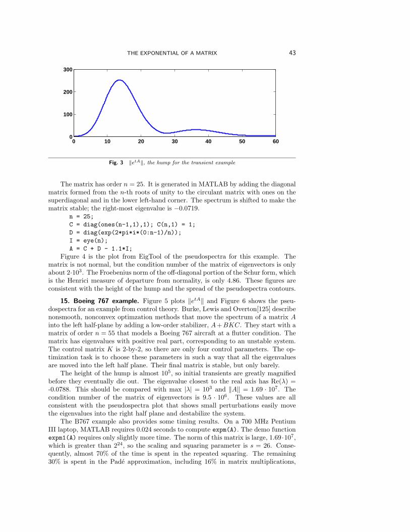
THE EXPONENTIAL OF A MATRIX 43
0 10 20 30 40 50 600
100
200
300
Fig. 3 ‖etA‖, the hump for the transient example
The matrix has order n = 25. It is generated in MATLAB by adding the diagonalmatrix formed from the n-th roots of unity to the circulant matrix with ones on thesuperdiagonal and in the lower left-hand corner. The spectrum is shifted to make thematrix stable; the right-most eigenvalue is −0.0719.
n = 25;C = diag(ones(n-1,1),1); C(n,1) = 1;D = diag(exp(2*pi*i*(0:n-1)/n));I = eye(n);A = C + D - 1.1*I;
Figure 4 is the plot from EigTool of the pseudospectra for this example. Thematrix is not normal, but the condition number of the matrix of eigenvectors is onlyabout 2·103. The Froebenius norm of the off-diagonal portion of the Schur form, whichis the Henrici measure of departure from normality, is only 4.86. These figures areconsistent with the height of the hump and the spread of the pseudospectra contours.
15. Boeing 767 example. Figure 5 plots ‖etA‖ and Figure 6 shows the pseu-dospectra for an example from control theory. Burke, Lewis and Overton[125] describenonsmooth, nonconvex optimzation methods that move the spectrum of a matrix Ainto the left half-plane by adding a low-order stabilizer, A+BKC. They start with amatrix of order n = 55 that models a Boeing 767 aircraft at a flutter condition. Thematrix has eigenvalues with positive real part, corresponding to an unstable system.The control matrix K is 2-by-2, so there are only four control parameters. The op-timization task is to choose these parameters in such a way that all the eigenvaluesare moved into the left half plane. Their final matrix is stable, but only barely.
The height of the hump is almost 105, so initial transients are greatly magnifiedbefore they eventually die out. The eigenvalue closest to the real axis has Re(λ) =-0.0788. This should be compared with max |λ| = 103 and ‖A‖ = 1.69 · 107. Thecondition number of the matrix of eigenvectors is 9.5 · 106. These values are allconsistent with the pseudospectra plot that shows small perturbations easily movethe eigenvalues into the right half plane and destabilize the system.
The B767 example also provides some timing results. On a 700 MHz PentiumIII laptop, MATLAB requires 0.024 seconds to compute expm(A). The demo functionexpm1(A) requires only slightly more time. The norm of this matrix is large, 1.69 ·107,which is greater than 224, so the scaling and squaring parameter is s = 26. Conse-quently, almost 70% of the time is spent in the repeated squaring. The remaining30% is spent in the Pade approximation, including 16% in matrix multiplications,

44 CLEVE MOLER AND CHARLES VAN LOAN
−3 −2.5 −2 −1.5 −1 −0.5 0 0.5−2
−1.5
−1
−0.5
0
0.5
1
1.5
2
dim = 25−4
−3.5
−3
−2.5
−2
−1.5
−1
Fig. 4 ε-pseudospectra for the transient example
0 10 20 30 40 50 600
2
4
6
8
10x 10
4
Fig. 5 ‖etA‖, the hump for the stabilized Boeing 767
A*X, and 11% in the “matrix division”, D\E. By way of comparison, the computa-tion of eigenvalues and eigenvectors with [V,D] = eig(A) on this machine requires0.020 seconds, so for this example, computation of the exponential of a matrix takesabout the same time as computation of its eigenvalues and eigenvectors. However, ast increases, the time required to compute expm(t*A) also increases, while the timerequired to compute eig(t*A) does not change very much.
Acknowledgments. Thanks to the editors of SIAM Review for republishing Nine-teen Ways and, especially, to Randy LeVeque for his valuable contributions.

THE EXPONENTIAL OF A MATRIX 45
−100 −50 0 50−100
−80
−60
−40
−20
0
20
40
60
80
100
dim = 55−5
−4.5
−4
−3.5
−3
−2.5
−2
Fig. 6 ε-pseudospectra for the stabilized Boeing 767
REFERENCES
[123] M. Arioli, B. Codenotti, and C. Fassino, The Pade method for computing the matrixexponential, Lin. Alg. Applic. 240 (1996), 111–130.
[124] P. Bochev and S. Markov, A self-validating numerical method for the matrix exponential,J. Computing, 43 (1989), pp. 59–72.
[125] J. V. Burke, A. S. Lewis and M. L. Overton, A Nonsmooth, Nonconvex OptimizationApproach to Robust Stabilization by Static Output Feedback and Low-Order Controllers,submitted to 4th IFAC Symposium on Robust Control Design (2003).
[126] D. Calvetti, E. Gallopoulos, and L. Reichel, Incomplete partial fractions for parallelevaluation of rational matrix functions, J. Comput. Appl. Math., 59 (1995), pp. 349–380.
[127] E. Celledoni and A. Iserles, Approximating the exponential from a Lie algebra to a Liegroup, Math. Comp. 69 (2000), pp. 1457–1480.
[128] E. Celledoni and A. Iserles, Methods for the approximation of the matrix exponential in aLie-algebraic setting, IMA J. Numer. Anal., 21 (2001), pp. 463–488.
[129] S.H. Chung, N.J. Higham, C.S. Kenney, and A.J. Laub, Approximating the logarithm of amatrix to specified accuracy, SIAM J. Matrix Anal. Appl., 22 (2001), pp. 1112–1125.
[130] L. Dieci and A. Papini, Pade Approximation for the Exponential of a Block Triangular Matrix,Lin. Alg. Applic., 308 (2000), pp. 183-202.
[131] L. Dieci and A. Papini, Conditioning of the Exponential of a Block Triangular Matrix, J.Num. Alg., 28 (2001), pp. 137-150.
[132] V. L. Druskin and L. A. Knizhnerman, Krylov space approximations of eigenpairs andmatrix functions in exact and computer arithmetic, Numer. Linear Algebra Appl. 2 (1995),pp. 205-217.
[133] V. Druskin, A. Greenbaum, and L. Knizhnerman, Using nonorthogonal Lanczos vectors inthe computation of matrix functions, SIAM J. Sci. Comput., 19 (1998), pp. 38–54.
[134] W.S. Edwards, L.S. Tuckerman, R.A. Friesner, and D.C. Sorensen, Krylov methods forthe incompressible Navier Stokes equations, J. Comput. Phys., 110 (1994), pp. 82–102.
46 CLEVE MOLER AND CHARLES VAN LOAN
[135] M. Embree and L. N. Trefethen, Pseudospectra Gateway,http://web.comlab.ox.ac.uk/pseudospectra
[136] E. Gallopoulos and Y. Saad, Efficient solution of parabolic equations by Krylov approxi-mation methods, SIAM J. Sci. Statist. Comput, 13 (1992), pp. 1236–1264.
[137] N. J. Higham, Evaluating Pade approximants of the matrix logarithm, SIAM J. Matrix Anal.Appl., 22 (2001), pp. 1126–1135.
[138] M. Hochbruck and C. Lubich, On Krylov subspace approximations to the matrix exponential,SIAM J. Numer. Anal., 34 (1997), pp. 1911–1925.
[139] M. Hochbruck, C. Lubich and H. Selhofer, Exponential integrators for large systems ofdifferential equations, SIAM J. Sci. Comput., 19 (1998), pp. 1552–1574.
[140] T. Jahnke and C. Lubich, Error bounds for exponential operator splittings, BIT 40 (2000),pp. 735–744.
[141] C. Kenney and A. J. Laub, Condition estimates for matrix functions, SIAM J. Matrix Anal.Appl., 10 (1989), pp. 191–209.
[142] C. Kenney and A. J. Laub, Small-sample statistical condition estimates for general matrixfunctions, SIAM J. Sci. Comput., 15 (1995), pp. 36–61.
[143] C. S. Kenney and A. J. Laub, A Schur–Frechet Algorithm for Computing the Logarithm andExponential of a Matrix, SIAM J. Mat. Anal., 19 (1998), pp. 640-663.
[144] L. A. Knizhnerman, Calculation of functions of unsymmetric matrices using Arnoldi’smethod, Comput. Math. and Math. Phys., 31 (1991), pp. 1–9.
[145] R. Mathias, Condition estimation for matrix functions via the Schur decomposition, SIAMJ. Matrix Anal. Appl., 16 (1995), pp. 565–578.
[146] R. Mathias, Evaluating the Frechet derivative of the matrix exponential, Numer. Math., 63(1992), pp. 213–226.
[147] I. Najfeld and T.F. Havel, Derivatives of the matrix exponential and their computation,Adv. Appl. Math., 16 (1995), pp. 321–375.
[148] B. Nour-Omid, Applications of the Lanczos algorithm, Comput. Phys. Comm., 53 (1989), pp.157–168.
[149] Y. Saad, Analysis of some Krylov subspace approximations to the matrix exponential operator,SIAM J. Numer. Anal., 29 (1992), pp. 209–228.
[150] Q. Sheng, Global error estimates for exponential splitting, IMA J. Numer. Anal. 14 (1993),pp. 27–56.
[151] R. B. Sidje, Expokit: Software Package for Computing Matrix Exponentials, ACM Trans.Math. Software, 24 (1998), pp. 130–156.
[152] R. B. Sidje, Expokit software, http://www.maths.uq.edu.au/expokit.[143] R. B. Sidje and W.J. Stewart, A Survey of Methods for Computing Large Sparse Matrix
Exponentials Arising in Markov Chains, Computational Statistics and Data Analysis 29(1999), 345–368.
[154] D.E. Stewart and T.S. Leyk, Error estimates for Krylov subspace approximations of matrixexponentials, J. Comput. Appl. Math. 72 (1996), pp. 359–369.
[155] L. N. Trefethen, Pseudospectra of linear operators, SIAM Review 39 (1997), pp. 383-406.[156] L. N. Trefethen, Computation of pseudospectra, in Acta Numerica (1999), pp. 247-295,
Cambridge University Press.[157] T. G. Wright, EigTool software package,
http://web.comlab.ox.ac.uk/projects/pseudospectra/eigtool/.[158] A. Zanna and H.Z. Munthe-Kaas, Generalized polar decompositions for the approximation
of the matrix exponential, SIAM J. Matrix Anal. Appl., 23 (2002), pp. 840–862.