GEOLOGI FOR SAMFUNNETGEOLOGY FOR SOCIETY

NGUNorges geologiske undersøkelseGeological Survey of Norway

Geological Survey of Norway

Postboks 6315 Sluppen

NO-7491 Trondheim, Norway

Tel.: 47 73 90 40 00

Telefax 47 73 92 16 20 REPORT

Report no.: 2014.052

ISSN 0800-3416

Grading: Open

Title:

Helicopter-borne magnetic, electromagnetic and radiometric geophysical survey in the Hjartdal-Rjukan-

Flesberg area, Telemark and Buskerud.

Authors: Alexei Rodionov, Frode Ofstad,

Alexandros Stampolidis & Georgios Tassis.

Client:

NGU

County:

Telemark and Buskerud Municipalities:

Hjartdal, Tinn, Notodden, Rollag og Flesberg

Map-sheet name (M=1:250.000)

SKIEN Map-sheet no. and -name (M=1:50.000)

1614 I Tinnsjø, 1614 II Gransherad, 1614 III Flatdal.

1614 IV Rjukan, 1714 III Notodden, 1714 IV Flesberg

Deposit name and grid-reference:

Tinnoset UTM 32 W 501800 – 6620800

Number of pages: 29 Price (NOK): 120,- Map enclosures:

Fieldwork carried out:

October-November 2013

October-November 2014

Date of report:

December 2014 Project no.:

342900 Person responsible:

Summary:

NGU conducted an airborne geophysical survey in the Hjartdal-Rjukan-Flesberg area area in

October-November 2013, October-November 2014 as a part of the MINS project. This report describes

and documents the acquisition, processing and visualization of recorded datasets. The geophysical survey

results reported herein are 9700 line km, covering an area of 1940 km2.

The NGU modified Geotech Ltd. Hummingbird frequency domain system supplemented by optically

pumped Cesium magnetometer and a 1024 channels RSX-5 spectrometer was used for data acquisition.

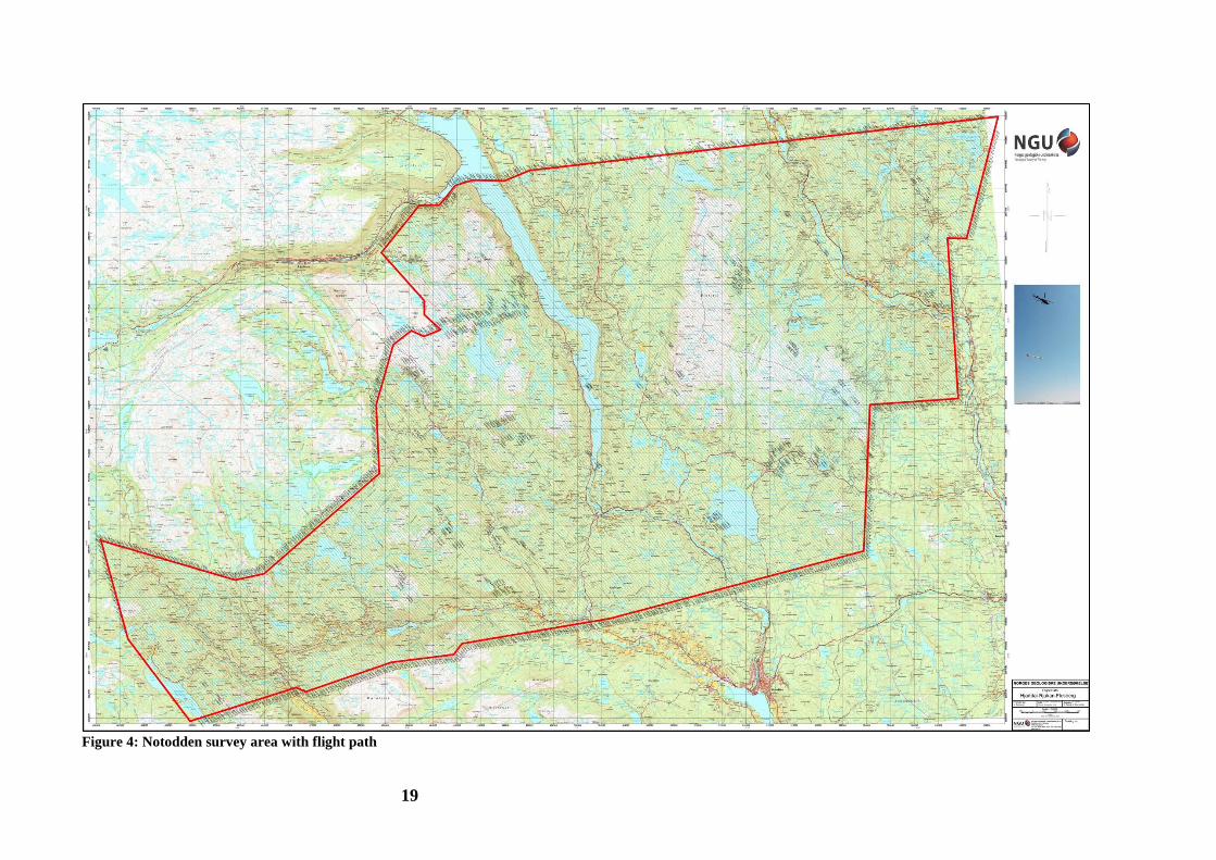
The survey was flown with 200 m line spacing, line direction 320o (Northeast to Southwest), 140

o

(Northwest to Southeast) and average speed 74 km/h. The average terrain clearance of the bird was 57 m.

Collected data were processed by AR Geoconsulting using Geosoft Oasis Montaj software. Raw total

magnetic field data were corrected for diurnal variation and levelled using standard micro levelling

algorithm. Final grid was filtered using Butterworth filter.

EM data were filtered and levelled using both automated and manual levelling procedure. Apparent

resistivity was calculated from in-phase and quadrature data for two high frequencies (6606 and 7001

Hz), separately using homogeneous half space model. Apparent resistivity grids were filtered using 3x3

convolution filter. Resistivity was not calculated for low frequencies (880 and 980 Hz) due to low

signal/noise ratio and survey results presented as profile plots of in-phase and quadrature responses.

Radiometric data were processed using standard procedures recommended by International Atomic

Energy Association.

Data were gridded with the cell size of 50 x 50 m and presented as a shaded relief maps at the scale of

1:50000.

Keywords: Geophysics

Airborne

Magnetic

Electromagnetic

Gamma spectrometry

Radiometric

Technical report

Table of Contents 1. INTRODUCTION ............................................................................................................ 4 2. SURVEY SPECIFICATIONS ........................................................................................ 5

2.1 Airborne Survey Parameters .................................................................................... 5

2.2 Airborne Survey Instrumentation ........................................................................... 6

2.3 Airborne Survey Logistics Summary ...................................................................... 6

3. DATA PROCESSING AND PRESENTATION ........................................................... 7

3.1 Total Field Magnetic Data ........................................................................................ 7

3.2 Electromagnetic Data ................................................................................................ 9

3.3 Radiometric data ..................................................................................................... 10

4. PRODUCTS .................................................................................................................... 14 5. REFERENCES ............................................................................................................... 15

Appendix A1: Flow chart of magnetic processing.............................................................. 16 Appendix A2: Flow chart of EM processing ....................................................................... 16

Appendix A3: Flow chart of radiometry processing .......................................................... 16

FIGURES

Figure 1: Hjartdal-Rjukan-Flesberg area survey area ......................................................... 4

Figure 2: Hummingbird system in air .................................................................................... 7

Figure 3: Gamma-ray spectrum with the K, Th, U and Total count windows................. 10 Figure 4: Notodden survey area with flight path ................................................................ 19

Figure 5: Total Magnetic Field ............................................................................................. 20 Figure 6: Magnetic Vertical Derivative ................................................................................ 21 Figure 7: Magnetic Tilt Derivative ....................................................................................... 22 Figure 8: Apparent resistivity. Frequency 6600 Hz, Coplanar coils ................................. 23

Figure 9: In-phase and quadrature response. Frequency 880 Hz, coplanar coils ............ 24 Figure 10: Apparent resistivity. Frequency 7000 Hz, Coaxial coils .................................. 25

Figure 11: In-phase and quadrature response. Frequency 980 Hz, Coaxial coils ............ 26 Figure 12: Uranium ground concentration .......................................................................... 27 Figure 13: Thorium ground concentration .......................................................................... 28

Figure 14: Potassium ground concentration ........................................................................ 29

Figure 15: Radiometric Ternary map .................................................................................. 30

TABLES

Table 1. Instrument Specifications ......................................................................................... 6 Table 2. Hummingbird electromagnetic system, frequency and coil configurations ......... 6

Table 3: Specified channel windows and energy spectrum for the RSX-5 systems used in

this survey ............................................................................................................................... 11 Table 4. Maps in scale 1:50000 available from NGU on request. ...................................... 14

4

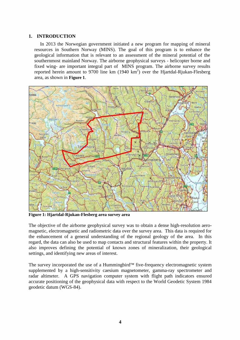
1. INTRODUCTION

In 2013 the Norwegian government initiated a new program for mapping of mineral

resources in Southern Norway (MINS). The goal of this program is to enhance the

geological information that is relevant to an assessment of the mineral potential of the

southernmost mainland Norway. The airborne geophysical surveys - helicopter borne and

fixed wing- are important integral part of MINS program. The airborne survey results

reported herein amount to 9700 line km (1940 km2) over the Hjartdal-Rjukan-Flesberg

area, as shown in Figure 1.

Figure 1: Hjartdal-Rjukan-Flesberg area survey area

The objective of the airborne geophysical survey was to obtain a dense high-resolution aero-

magnetic, electromagnetic and radiometric data over the survey area. This data is required for

the enhancement of a general understanding of the regional geology of the area. In this

regard, the data can also be used to map contacts and structural features within the property. It

also improves defining the potential of known zones of mineralization, their geological

settings, and identifying new areas of interest.

The survey incorporated the use of a Hummingbird five-frequency electromagnetic system

supplemented by a high-sensitivity caesium magnetometer, gamma-ray spectrometer and

radar altimeter. A GPS navigation computer system with flight path indicators ensured

accurate positioning of the geophysical data with respect to the World Geodetic System 1984

geodetic datum (WGS-84).

5

2. SURVEY SPECIFICATIONS

2.1 Airborne Survey Parameters

NGU used a modified Hummingbird electromagnetic and magnetic helicopter survey

system designed to obtain low level, slow speed, detailed airborne magnetic and

electromagnetic data (Geotech 1997). The system was supplemented by 1024 channel

gamma-ray spectrometer which was used to map ground concentrations of U, Th and K.

The airborne survey began on October 16th

2013 and was cancelled on November 11th

due to

bad weather. It was continued on October 12th

2014 and completed on November 5th

2014. A

Eurocopter AS350-B3 helicopter from helicopter company HeliScan AS was used to tow the

bird. The survey lines were spaced 200 m apart. Lines were oriented at a 140 azimuth (UTM

zone 32W coordinates).

The magnetic and electromagnetic sensors are housed in a single 7.5 m long bird, which was

maintained at an average of 57 m above the topographic surface. A gamma-ray spectrometer,

installed under the belly of the helicopter, registered natural gamma ray radiation

simultaneously with the acquisition of magnetic/EM data.

Just before the start of the first survey of 2014 field season, instrumental problems were

discovered. The highest frequency (34 kHz) was not stable, and this instability influenced on

the quality of the other frequencies. To be able to collect data for the four lowest frequencies,

it was decided not to transmit on 33.4 kHz.

Rugged terrain and abrupt changes in topography affected the aircraft pilot’s ability to ‘drape’

the terrain; therefore the average instrumental height was higher than the standard survey

instrumental height, which is defined as 30 m plus a height of obstacles (trees, power lines

etc.) for EM and magnetic sensors.

The ground speed of the aircraft varied from 35 – 110 km/h depending on topography, wind

direction and its magnitude. On average, the ground speed during measurements is calculated

to 74 km/h. Magnetic data were recorded at 0.2 second intervals resulting in approximately

4 m point spacing. EM data were recorded at 0.1 second intervals resulting in data with a

sample increment of 2 m along the ground in average. Spectrometry data were recorded every

1 second giving a point spacing of approximately 20 meters. The above parameters allow

recognizing sufficient detail in the data to detect subtle anomalies that may represent

mineralization and/or rocks of different lithological and petrophysical composition.

A base magnetometer to monitor diurnal variations in the magnetic field was located at

Notodden (UTM 510500 – 6602800) in 2013 and at Jondalen (UTM 531200 – 6619200) in

2014. GEM GSM-19 station magnetometer data were recorded once every 3 seconds. The

CPU clock of the base magnetometer and the helicopter magnetometer were both

synchronized to UTC (Universal Time Coordinates) through the built-in GPS receiver to

allow correction of diurnals.

Navigation system uses GPS/GLONASS satellite tracking systems to provide real-time WGS-

84 coordinate locations for every second. The accuracy achieved with no differential

corrections is reported to be less than 5 m in the horizontal directions. The GPS receiver

antenna was mounted externally to the tail tip of the helicopter.

6

For quality control, the electromagnetic, magnetic and radiometric, altitude and navigation

data were monitored on four separate windows in the operator's display during flight while

they were recorded in three data ASCII streams to the PC hard disk drive. Spectrometry data

were also recorded to an internal hard drive of the spectrometer. The data files were

transferred to the field workstation via USB flash drive. The raw data files were backed up

onto USB flash drive in the field.

2.2 Airborne Survey Instrumentation

Instrument specification is given in table 1. Frequencies and coil configuration for the

Hummingbird EM system is given in table 2.

Table 1. Instrument Specifications

Instrument Producer/Model Accuracy Sampling

frequency/interval

Magnetometer Scintrex Cs-2 0,002 nT 5 Hz

Base magnetometer GEM GSM-19 0.1 nT 3 sec

Electromagnetic Geotech Hummingbird 1 – 2 ppm 10 Hz

Gamma spectrometer Radiation Solutions

RSX-5

1024 channels, 16

liters down, 4 liters

up

1 Hz

Radar altimeter Bendix/King KRA 405B ± 3 % 0 – 500 feet

± 5 % 500 – 2500

feet

1 Hz

Pressure/temperature Honeywell PPT ± 0,03 % FS 1 Hz

Navigation Topcon GPS-receiver ± 5 meter 1 Hz

Acquisition system PC based in house

software

Table 2. Hummingbird electromagnetic system, frequency and coil configurations

Coils: Frequency Orientation Separation

A 7700 Hz Coaxial 6.20 m

B 6600 Hz Coplanar 6.20 m

C 980 Hz Coaxial 6.025 m

D 880 Hz Coplanar 6.025 m

2.3 Airborne Survey Logistics Summary

Traverse (survey) line spacing: 200 metres

Traverse line direction: 140 NE-SW

Nominal aircraft ground speed: 30 - 110 km/h

Average sensor terrain clearance EM+Mag: 57 metres

Average sensor terrain clearance Rad: 87 metres

Sampling rates: 0.2 seconds - magnetometer

0.1 seconds - electromagnetics

1.0 second - spectrometer, GPS, altimeter

7

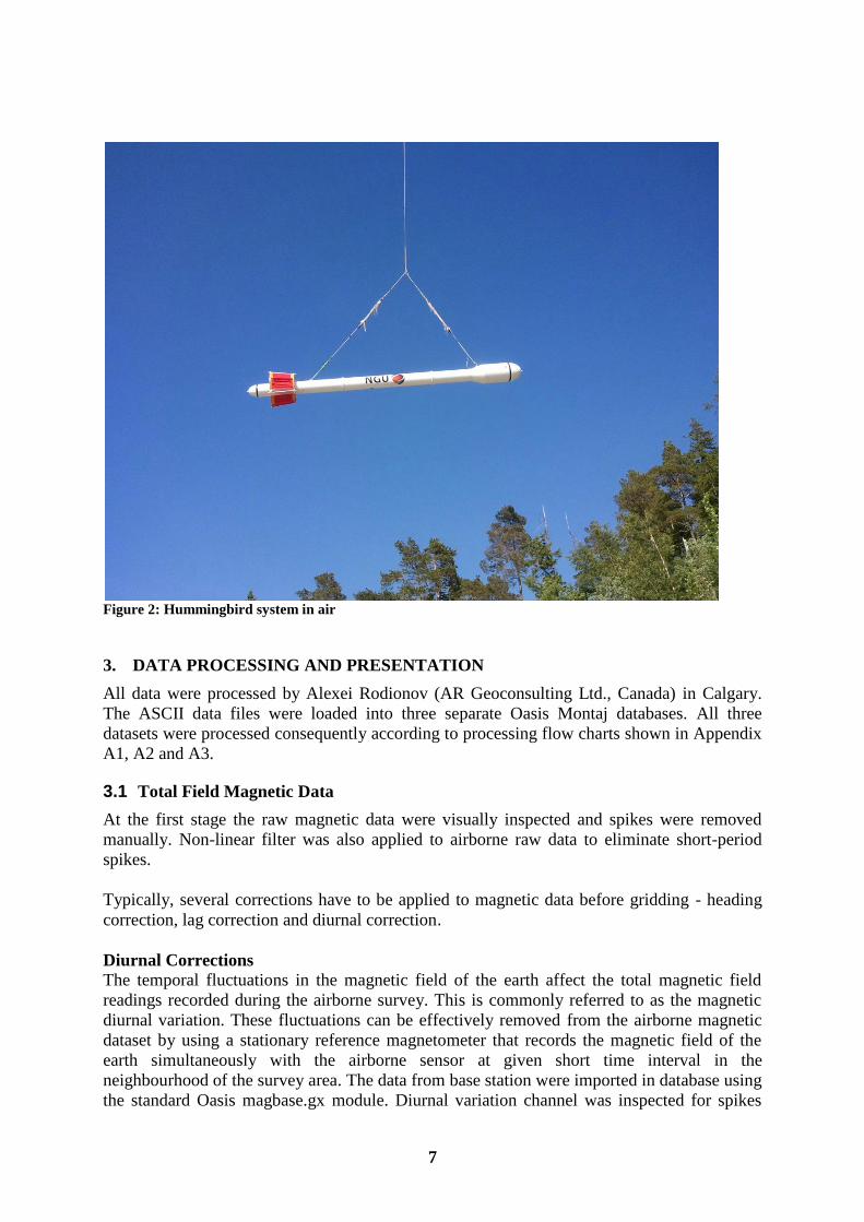
Figure 2: Hummingbird system in air

3. DATA PROCESSING AND PRESENTATION

All data were processed by Alexei Rodionov (AR Geoconsulting Ltd., Canada) in Calgary.

The ASCII data files were loaded into three separate Oasis Montaj databases. All three

datasets were processed consequently according to processing flow charts shown in Appendix

A1, A2 and A3.

3.1 Total Field Magnetic Data

At the first stage the raw magnetic data were visually inspected and spikes were removed

manually. Non-linear filter was also applied to airborne raw data to eliminate short-period

spikes.

Typically, several corrections have to be applied to magnetic data before gridding - heading

correction, lag correction and diurnal correction. Diurnal Corrections

The temporal fluctuations in the magnetic field of the earth affect the total magnetic field

readings recorded during the airborne survey. This is commonly referred to as the magnetic

diurnal variation. These fluctuations can be effectively removed from the airborne magnetic

dataset by using a stationary reference magnetometer that records the magnetic field of the

earth simultaneously with the airborne sensor at given short time interval in the

neighbourhood of the survey area. The data from base station were imported in database using

the standard Oasis magbase.gx module. Diurnal variation channel was inspected for spikes

8

and spikes were removed manually if necessary. Magnetic diurnals data were within the

standard NGU specifications during the entire survey (Rønning 2013).

Diurnal variations were measured with GEM GSM-19 magnetometer. The recorded data are

merged with the airborne data and the diurnal correction is applied according to equation (1).

BBTTc B BBB , (1)

where:

readingsstation Base

level base datum Average

readings field totalAirborne

readings field totalairborne Corrected

B

BB

T

Tc

B

B

B

Corrections for Lag and heading

Neither a lag nor cloverleaf tests were performed before the survey. According to previous

reports the lag between logged magnetic data and the corresponding navigational data was 1-2

fids. Translated to a distance it would be no more than 10 m - the value comparable with the

precision of GPS. A heading error for a towed system is usually either very small or non-

existent. So no lag and heading corrections were applied.

Magnetic data processing, gridding and presentation

The total field magnetic anomaly data ( TAB ) were calculated from the diurnal corrected data

( TcB ) after subtracting the IGRF for the surveyed area calculated for the data period (eq.2)

IGRFTcTA BB (2)

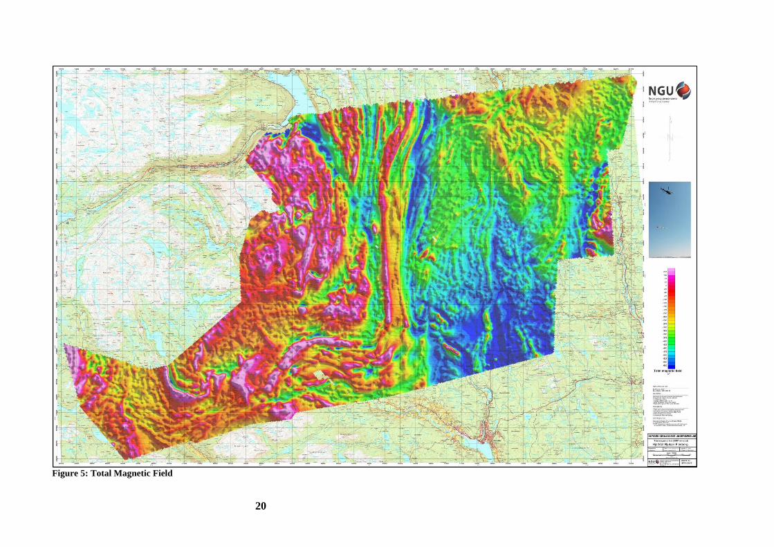
The total field anomaly data were gridded using a minimum curvature method with a grid cell

size of 50 meters. This cell size is equal to one quarter of the 200 m average line spacing. In

order to remove small line-to-line levelling errors that were detected on the gridded magnetic

anomaly data, the Geosoft Micro-levelling technique was applied on the flight line based

magnetic database. Then, the micro-levelled channel was gridded using again a minimum

curvature method with 50 m grid cell size. Finally, Butterworth filter was applied to reduce

“ringing” effect of gridding and smooth the grid.

The processing steps of magnetic data presented so far, were performed on point basis. The

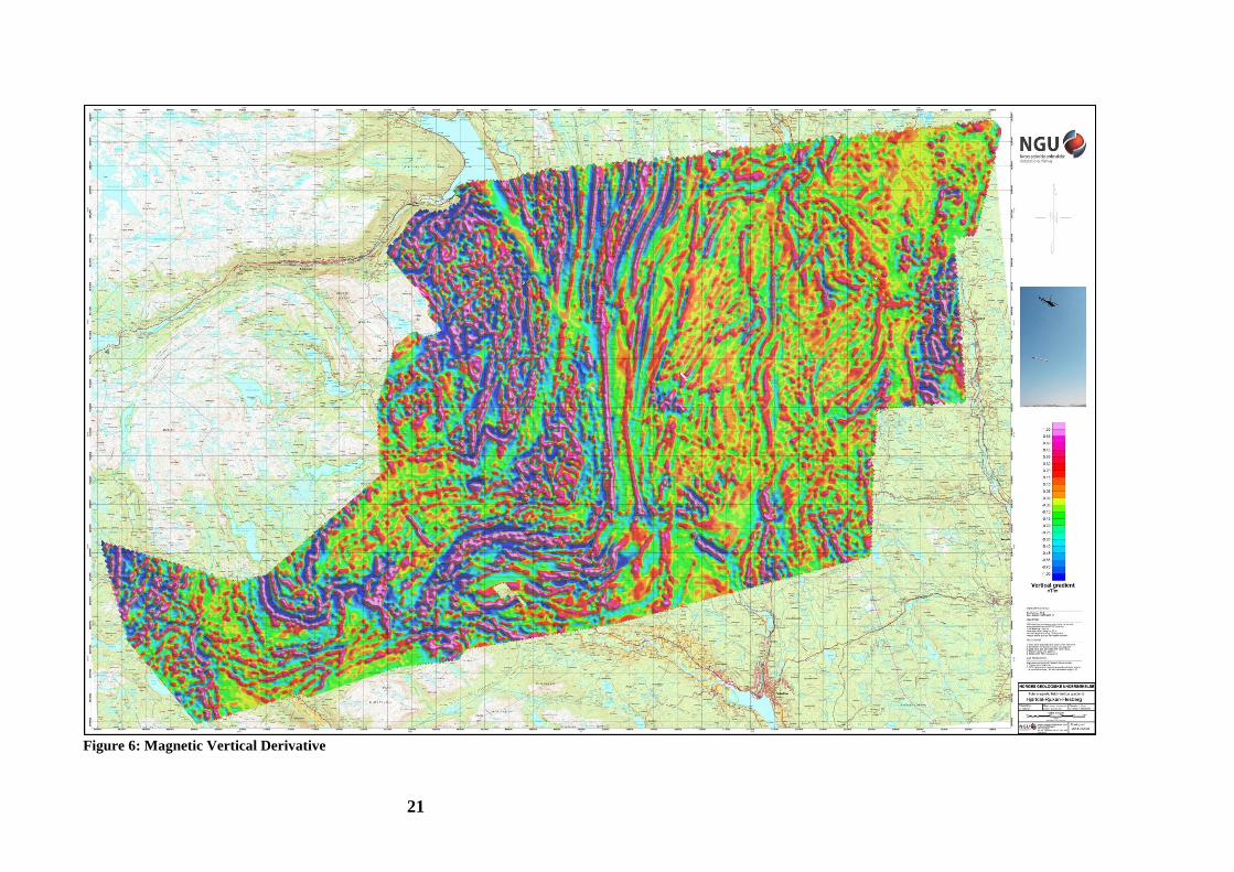
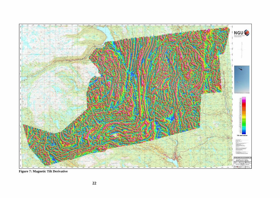
following steps are performed on grid basis. Vertical Gradient along with the Tilt Derivative

of the total magnetic anomaly was calculated from the micro-levelled total magnetic anomaly

grid. The Tilt derivative (TD) was calculated according to the equation (3)

HG

VGTD 1tan (3)

The results are presented in coloured shaded relief maps:

A. Total field magnetic anomaly

B. Vertical gradient of total magnetic anomaly

C. Tilt angle (or Tilt Derivative) of the total magnetic anomaly

9

These maps are representative of the distribution of magnetization over the surveyed areas.

The list of the produced maps is shown in Table 4.

3.2 Electromagnetic Data

The DAS computer records both an in-phase and a quadrature value for each of the four coil

sets of the electromagnetic system. Instrumental noise and drift should be removed before

computation of an apparent resistivity.

Instrumental noise

Noise level on all frequencies was above the survey specification during the whole survey.

Partially it was the result of swaying of the bird. The pendulum effect of a swaying was clear

visible on records especially on 880 Hz data. Presence of numerous habitations and power

lines introduced so called “cultural noise” which especially affected high frequencies. Lastly,

electronics malfunction also contributed to elevation of noise level. Traditionally used

combination of short non-linear filter and low pass filter could not suppress the noise. The

period of bird swaying – 3-8 sec. made application of low pass filter not effective. Low pass

filter, eliminating noise, also distorted a shape and amplitude of anomalies. To achieve

satisfactory results, spline approximation (B-spline filter) was applied to all data. Parameters

of filter were individually chosen for each flight and sometimes for separate lines.

Shifts of 7000 Ip and Q records, with amplitude of 15-20 ppm, was observed almost in all

flights, especially, in mountainous areas. Shifts were edited manually where it was possible.

Instrument Drift

In order to remove the effects of instrument drift caused by gradual temperature variations in

the transmitting and receiving circuits, background responses are recorded during each flight.

To obtain a background level the bird is raised to an altitude of at least 1000 ft above the

topographic surface so that no electromagnetic responses from the ground are present in the

recorded traces. The EM traces observed at this altitude correspond to a background (zero)

level of the system. If these background levels are recorded at 20-30 minute intervals, then the

drift of the system (assumed to be linear) can be removed from the data by resetting these

points to the initial zero level of the system. The drift must be removed on a flight-by-flight

basis, before any further processing is carried out. Geosoft HEM module was used for

applying drift correction. Residual instrumental drift, usually small, but non-linear, was

manually removed on line-to-line basis.

Instrumental drift during this survey was non-linear even in short time (3-5 min) intervals and

not within specifications (Rønning 2013) due to malfunction of Hummingbird electronics.

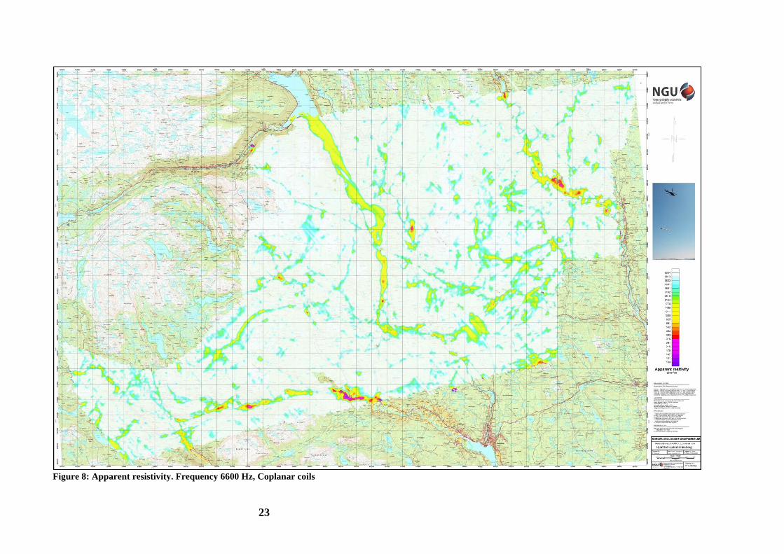
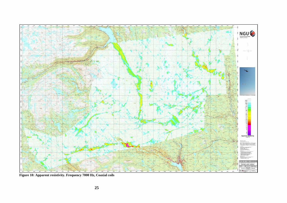
Apparent resistivity calculation and presentation

When levelling of the EM data was complete, apparent resistivity was calculated from in-

phase and quadrature EM components using a homogeneous half space model of the Earth

(Geosoft HEM module) for four frequencies 6600 and 7000 Hz. A threshold value of 1 ppm

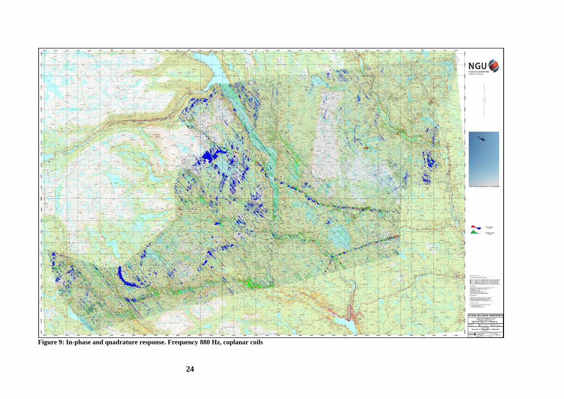
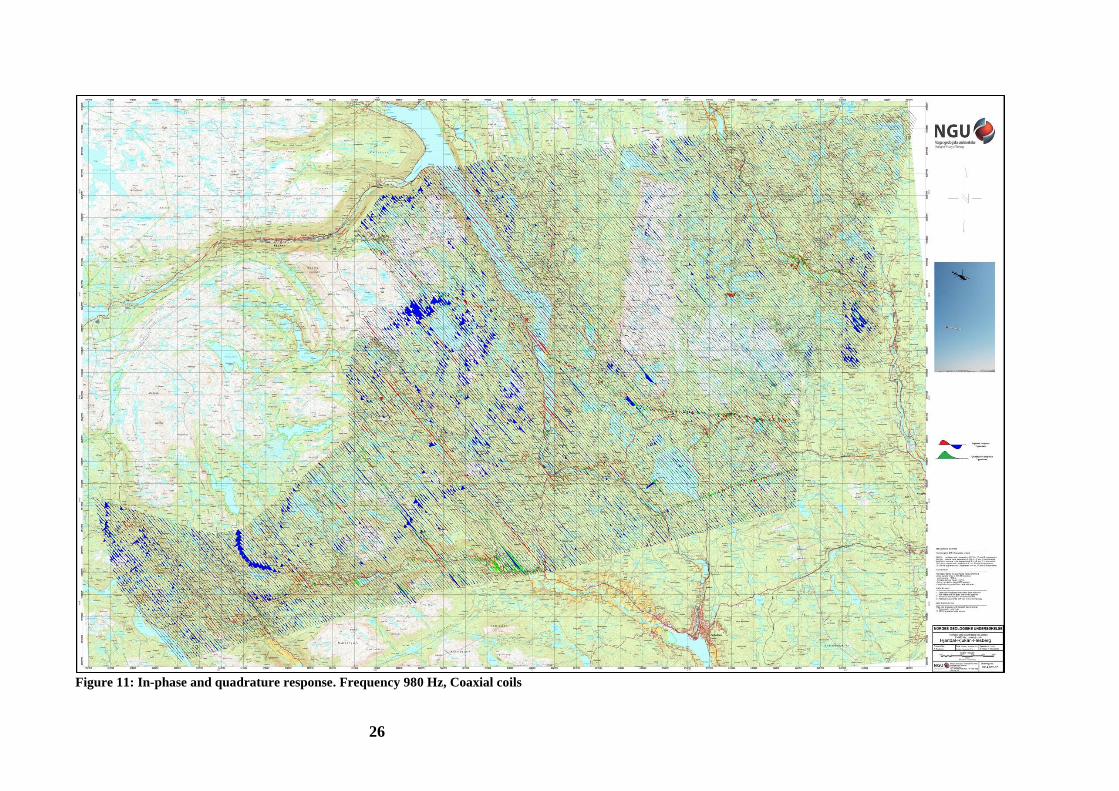
was set for inversion. Due to low signal to noise ratio, resistivity for 880 and 980 Hz was not

calculated. The 880 and 980 Hz data are presented as profile plots of in-phase and quadrature

responses. Note: Negative readings of in-phase component are controlled by high magnetic

susceptibility of rocks. 34000 Hz data covers only part of the survey area (2013 year survey)

and its results are not included in this report.

10

Secondary electromagnetic field decays rapidly with the distance (height of the sensors) – as

z-2

– z

-5 depending on the shape of the conductors and, at certain height, signals from the

ground sources become comparable with instrumental noise. Levelling errors or precision of

levelling can lead sometimes to appearance of artificial resistivity anomalies when data were

collected at high instrumental altitude. Application of threshold allows excluding such data

from an apparent resistivity calculation, though not completely. It’s particularly noticeable in

low frequencies datasets. Resistivity data were visually inspected; artificial anomalies

associated with high altitude measurements were manually removed.

Data, recorded at the height above 100 m were considered as non-reliable and removed from

presentation. Remaining resistivity data were gridded with a cell size 50 m and 3x3

convolution filter was applied to smooth resistivity grids.

3.3 Radiometric data

Airborne gamma-ray spectrometry measures the abundance of Potassium (K), Thorium (eTh),

and Uranium (eU) in rocks and weathered materials by detecting gamma-rays emitted due to

the natural radioelement decay of these elements. The data analysis method is based on the

IAEA recommended method for U, Th and K (International Atomic Energy Agency, 1991;

2003). A short description of the individual processing steps of that methodology as adopted

by NGU is given bellow:

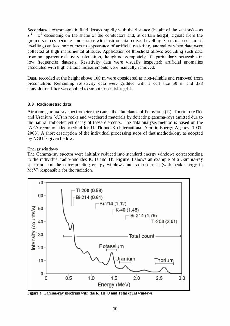
Energy windows

The Gamma-ray spectra were initially reduced into standard energy windows corresponding

to the individual radio-nuclides K, U and Th. Figure 3 shows an example of a Gamma-ray

spectrum and the corresponding energy windows and radioisotopes (with peak energy in

MeV) responsible for the radiation.

Figure 3: Gamma-ray spectrum with the K, Th, U and Total count windows.

11

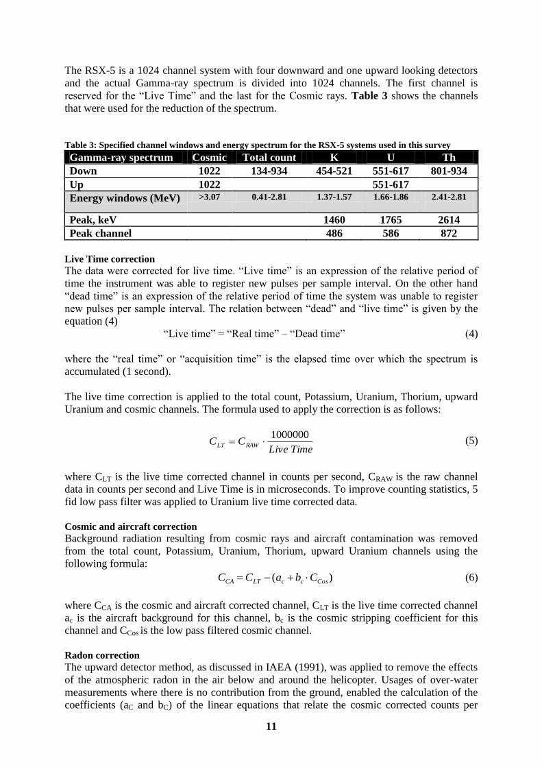
The RSX-5 is a 1024 channel system with four downward and one upward looking detectors

and the actual Gamma-ray spectrum is divided into 1024 channels. The first channel is

reserved for the “Live Time” and the last for the Cosmic rays. Table 3 shows the channels

that were used for the reduction of the spectrum.

Table 3: Specified channel windows and energy spectrum for the RSX-5 systems used in this survey

Gamma-ray spectrum Cosmic Total count K U Th

Down 1022 134-934 454-521 551-617 801-934

Up 1022 551-617

Energy windows (MeV) >3.07 0.41-2.81 1.37-1.57 1.66-1.86 2.41-2.81

Peak, keV 1460 1765 2614

Peak channel 486 586 872

Live Time correction

The data were corrected for live time. “Live time” is an expression of the relative period of

time the instrument was able to register new pulses per sample interval. On the other hand

“dead time” is an expression of the relative period of time the system was unable to register

new pulses per sample interval. The relation between “dead” and “live time” is given by the

equation (4)

“Live time” = “Real time” – “Dead time” (4)

where the “real time” or “acquisition time” is the elapsed time over which the spectrum is

accumulated (1 second).

The live time correction is applied to the total count, Potassium, Uranium, Thorium, upward

Uranium and cosmic channels. The formula used to apply the correction is as follows:

TimeLiveCC RAWLT

1000000 (5)

where CLT is the live time corrected channel in counts per second, CRAW is the raw channel

data in counts per second and Live Time is in microseconds. To improve counting statistics, 5

fid low pass filter was applied to Uranium live time corrected data.

Cosmic and aircraft correction

Background radiation resulting from cosmic rays and aircraft contamination was removed

from the total count, Potassium, Uranium, Thorium, upward Uranium channels using the

following formula:

)( CosccLTCA CbaCC (6)

where CCA is the cosmic and aircraft corrected channel, CLT is the live time corrected channel

ac is the aircraft background for this channel, bc is the cosmic stripping coefficient for this

channel and CCos is the low pass filtered cosmic channel.

Radon correction

The upward detector method, as discussed in IAEA (1991), was applied to remove the effects

of the atmospheric radon in the air below and around the helicopter. Usages of over-water

measurements where there is no contribution from the ground, enabled the calculation of the

coefficients (aC and bC) of the linear equations that relate the cosmic corrected counts per

12

second of Uranium channel with total count, Potassium, Thorium and Uranium upward

channels over water. Data over-land was used in conjunction with data over-water to calculate

the a1 and a2 coefficients used in equation (7) for the determination of the Radon component

in the downward uranium window:

ThU

UThCACACAU

aaaa

bbaThaUaUupRadon

21

221 (7)

where Radonu is the radon component in the downward uranium window, UupCA is the

filtered upward uranium, UCA is the filtered Uranium, ThCA is the filtered Thorium, a1, a2, aU

and aTh are proportional factors and bU an bTh are constants determined experimentally.

The effects of Radon in the downward Uranium are removed by simply subtracting RadonU

from UCA. The effects of radon in the other channels are removed using the following

formula:

)( CUCCARC bRadonaCC (8)

where CRC is the Radon corrected channel, CCA is the cosmic and aircraft corrected channel,

RadonU is the Radon component in the downward uranium window, aC is the proportionality

factor and bC is the constant determined experimentally for this channel from over-water data.

Compton Stripping

Potassium, Uranium and Thorium Radon corrected channels, are subjected to spectral overlap

correction. Compton scattered gamma rays in the radio-nuclides energy windows were

corrected by window stripping using Compton stripping coefficients determined from

measurements on calibrations pads at the Geological Survey of Norway in Trondheim (for

values, see Appendix A3).

The stripping corrections are given by the following formulas:

bbggA aa11 (9)

1

1

A

gbKbUgThU RCRCRC

ST

(10)

1

aa1

A

bgKbUgThTh RCRCRC

ST

(11)

1

a1a

A

KUThK RCRCRC

ST

(12)

where URC, ThRC, KRC are the radon corrected Uranium, Thorium and Potassium and a, b, g,

α, β, γ are Compton stripping coefficients.

Reduction to Standard Temperature and Pressure

The radar altimeter data were converted to effective height (HSTP) using the acquired

temperature and pressure data, according to the expression:

25.101315.273

15.273 P

THH STP

(13)

13

where H is the smoothed observed radar altitude in meters, T is the measured air temperature

in degrees Celsius and P is the measured barometric pressure in millibars.

Height correction

Variations caused by changes in the aircraft altitude relative to the ground was corrected to a

nominal height of 60 m. Data recorded at the height above 150 m were considered as non-

reliable and removed from processing. Total count, Uranium, Thorium and Potassium

stripped channels were subjected to height correction according to the equation:

STPht HC

STm eCC

60

60 (14)

where CST is the stripped corrected channel, Cht is the height attenuation factor for that

channel and HSTP is the effective height.

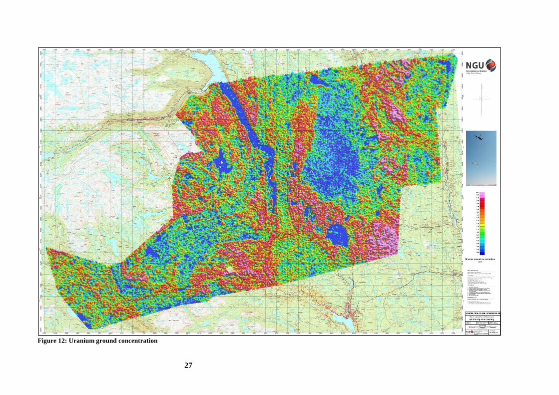
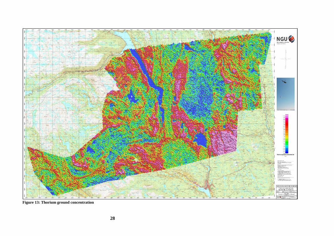
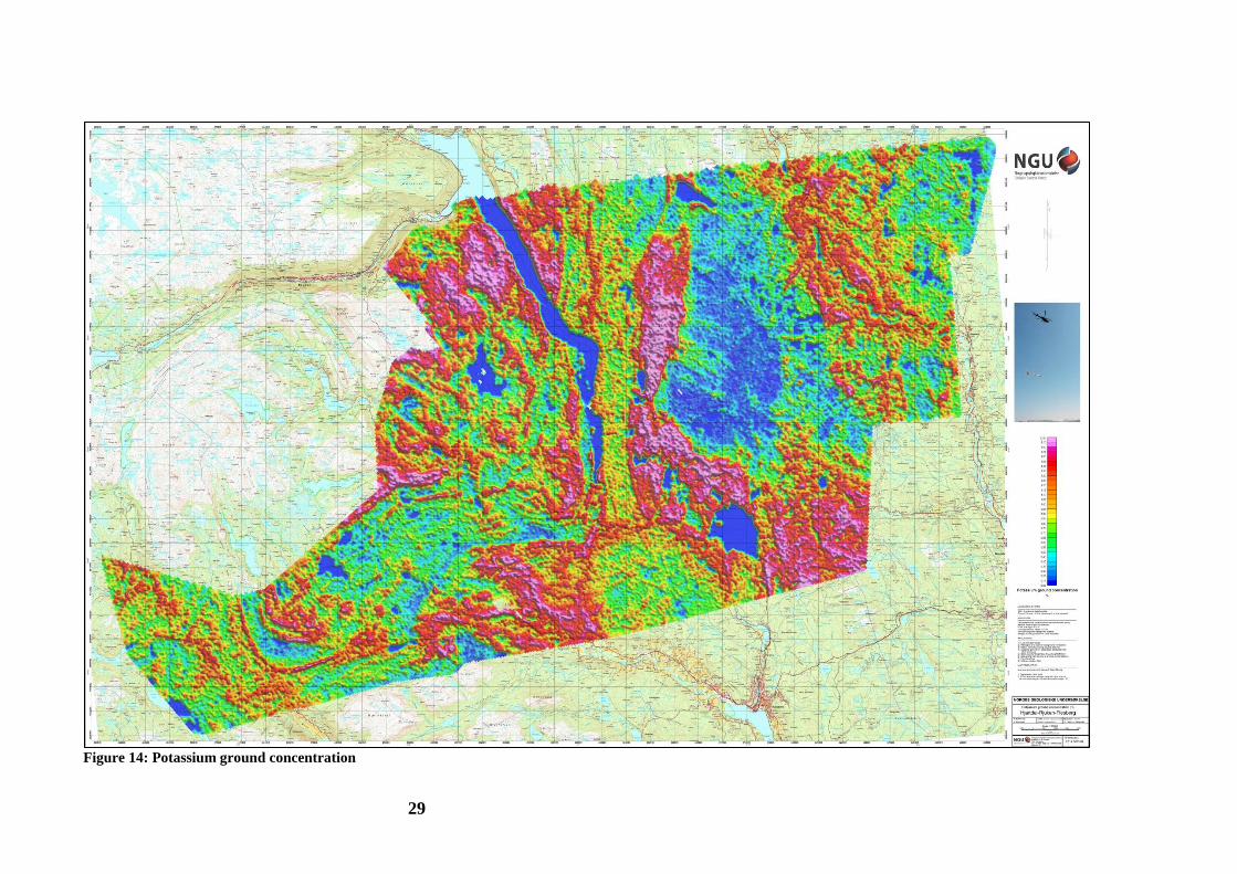
Conversion to ground concentrations

Finally, corrected count rates were converted to effective ground element concentrations

using calibration values derived from calibration pads at the Geological Survey of Norway in

Trondheim (for values, see Appendix A3). The corrected data provide an estimate of the

apparent surface concentrations of Potassium, Uranium and Thorium (K, eU and eTh).

Potassium concentration is expressed as a percentage, equivalent Uranium and Thorium as

parts per million (ppm). Uranium and Thorium are described as “equivalent” since their

presence is inferred from gamma-ray radiation from daughter elements (214

Bi for Uranium, 208

TI for Thorium). The concentration of the elements is calculated according to the following

expressions:

mSENSmCONC CCC 60_60 / (15)

where C60m is the height corrected channel, CSENS_60m is experimentally determined sensitivity

reduced to the nominal height (60m).

Spectrometry data gridding and presentation

Gamma-rays from Potassium, Thorium and Uranium emanate from the uppermost 30 to 40

centimetres of soil and rocks in the crust (Minty, 1997). Variations in the concentrations of

these radioelements largely related to changes in the mineralogy and geochemistry of the

Earth’s surface.

The spectrometry data were stored in a database and the ground concentrations were

calculated following the processing steps. A list of the parameters used in these steps is given

in Appendix A3.

Then the data were split in lines and ground concentrations of the three main natural radio-

elements Potassium, Thorium and Uranium and total gamma-ray flux (total count) were

gridded using a minimum curvature method with a grid cell size of 50 meters. In order to

remove small line-to-line levelling errors appeared on those grids, the data were micro-

levelled as in the case of the magnetic data, and re-gridded with the same grid cell size.

Finally, a 3x3 convolution filter was applied to Uranium grid to smooth the microlevelled

concentration grids.

Quality of the radiometric data was within standard NGU specifications (Rønning 2013). For

further reading regarding standard processing of airborne radiometric data, we recommend the

publications from Minty et al. (1997).

14

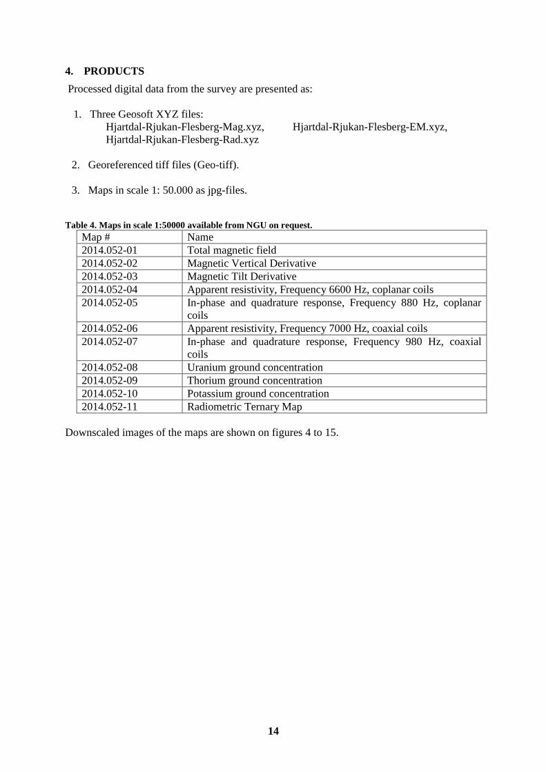
4. PRODUCTS

Processed digital data from the survey are presented as:

1. Three Geosoft XYZ files:

Hjartdal-Rjukan-Flesberg-Mag.xyz, Hjartdal-Rjukan-Flesberg-EM.xyz,

Hjartdal-Rjukan-Flesberg-Rad.xyz

2. Georeferenced tiff files (Geo-tiff).

3. Maps in scale 1: 50.000 as jpg-files.

Table 4. Maps in scale 1:50000 available from NGU on request.

Map # Name

2014.052-01 Total magnetic field

2014.052-02 Magnetic Vertical Derivative

2014.052-03 Magnetic Tilt Derivative

2014.052-04 Apparent resistivity, Frequency 6600 Hz, coplanar coils

2014.052-05 In-phase and quadrature response, Frequency 880 Hz, coplanar

coils

2014.052-06 Apparent resistivity, Frequency 7000 Hz, coaxial coils

2014.052-07 In-phase and quadrature response, Frequency 980 Hz, coaxial

coils

2014.052-08 Uranium ground concentration

2014.052-09 Thorium ground concentration

2014.052-10 Potassium ground concentration

2014.052-11 Radiometric Ternary Map

Downscaled images of the maps are shown on figures 4 to 15.

15

5. REFERENCES

Geosoft 2010: Montaj MAGMAP Filtering, 2D-Frequency Domain Processing of Potential Field

Data, Extension for Oasis Montaj v 7.1, Geosoft Corporation

Grasty, R.L., Holman, P.B. & Blanchard 1991: Transportable Calibration pads for ground and

airborne Gamma-ray Spectrometers. Geological Survey of Canada, Paper 90-23: 62 pp.

IAEA 1991: Airborne Gamma-Ray Spectrometry Surveying, Technical Report No 323, Vienna,

Austria, 97 pp.

IAEA 2003: Guidelines for radioelement mapping using gamma ray spectrometry data. IAEA-

TECDOC-1363, Vienna, Austria, 173 pp.

Minty, B.R.S. 1997: The fundamentals of airborne gamma-ray spectrometry. AGSO Journal of

Australian Geology and Geophysics, 17 (2): 39-50.

Minty, B.R.S., Luyendyk, A.P.J. and Brodie, R.C. 1997: Calibration and data processing for

gamma-ray spectrometry. AGSO Journal of Australian Geology and Geophysics, 17(2): 51-62.

Naudy, H. and Dreyer, H. 1968: Non-linear filtering applied to aeromagnetic profiles. Geophysical

Prospecting, 16(2): 171-178.

Rønning, J.S. 2013: NGUs helikoptermålinger. Plan for sikring og kontroll av datakvalitet. NGU

Intern rapport 2013.001, (38 sider).

16

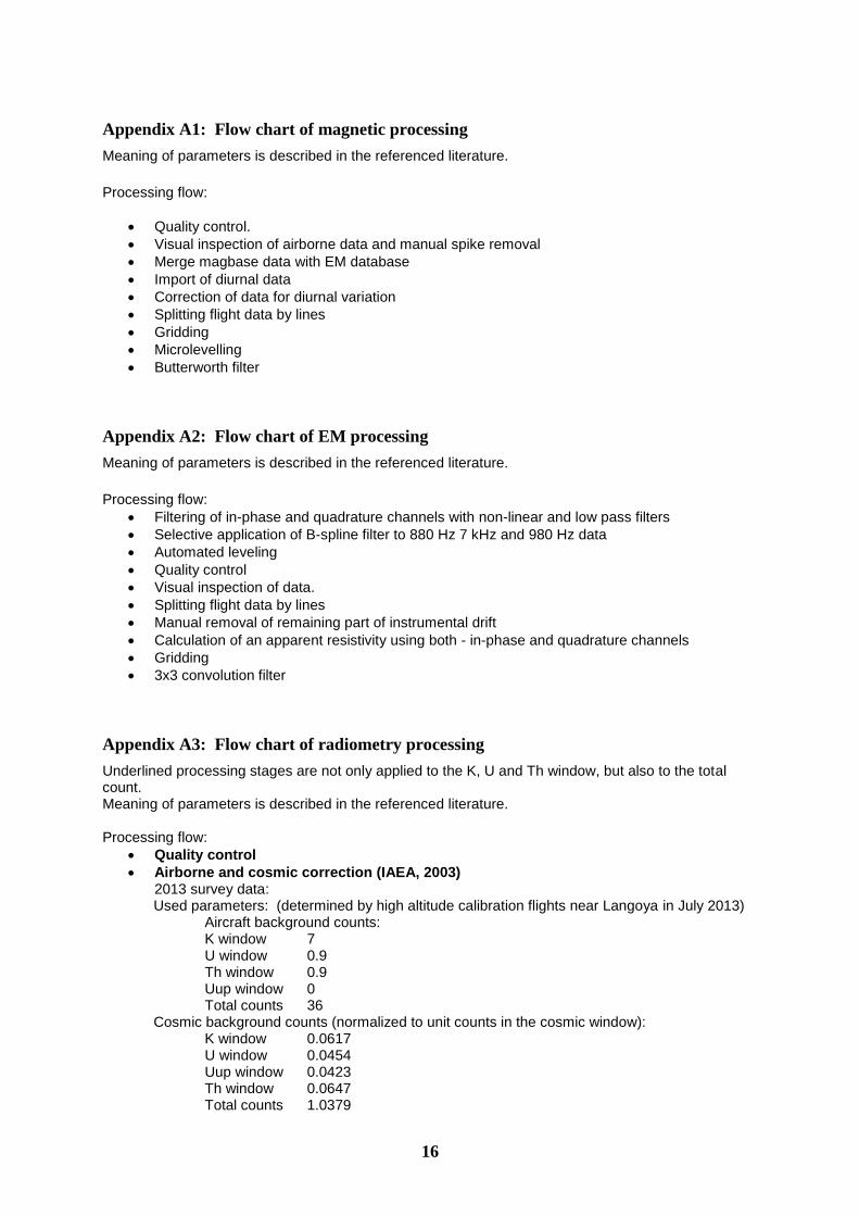
Appendix A1: Flow chart of magnetic processing

Meaning of parameters is described in the referenced literature.

Processing flow:

Quality control.

Visual inspection of airborne data and manual spike removal

Merge magbase data with EM database

Import of diurnal data

Correction of data for diurnal variation

Splitting flight data by lines

Gridding

Microlevelling

Butterworth filter

Appendix A2: Flow chart of EM processing

Meaning of parameters is described in the referenced literature.

Processing flow:

Filtering of in-phase and quadrature channels with non-linear and low pass filters

Selective application of B-spline filter to 880 Hz 7 kHz and 980 Hz data

Automated leveling

Quality control

Visual inspection of data.

Splitting flight data by lines

Manual removal of remaining part of instrumental drift

Calculation of an apparent resistivity using both - in-phase and quadrature channels

Gridding

3x3 convolution filter

Appendix A3: Flow chart of radiometry processing

Underlined processing stages are not only applied to the K, U and Th window, but also to the total count. Meaning of parameters is described in the referenced literature. Processing flow:

Quality control

Airborne and cosmic correction (IAEA, 2003) 2013 survey data:

Used parameters: (determined by high altitude calibration flights near Langoya in July 2013) Aircraft background counts: K window 7 U window 0.9 Th window 0.9 Uup window 0 Total counts 36 Cosmic background counts (normalized to unit counts in the cosmic window): K window 0.0617

U window 0.0454 Uup window 0.0423 Th window 0.0647 Total counts 1.0379

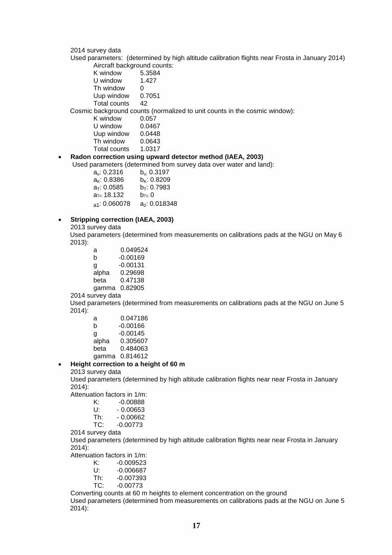
17

2014 survey data Used parameters: (determined by high altitude calibration flights near Frosta in January 2014)

Aircraft background counts: K window 5.3584 U window 1.427 Th window 0 Uup window 0.7051 Total counts 42 Cosmic background counts (normalized to unit counts in the cosmic window): K window 0.057

U window 0.0467 Uup window 0.0448 Th window 0.0643 Total counts 1.0317

Radon correction using upward detector method (IAEA, 2003) Used parameters (determined from survey data over water and land): au: 0.2316 bu: 0.3197 aK: 0.8386 bK: 0.8209 aT: 0.0585 bT: 0.7983 aTc: 18.132 bTc: 0

a1: 0.060078 a2: 0.018348

Stripping correction (IAEA, 2003) 2013 survey data Used parameters (determined from measurements on calibrations pads at the NGU on May 6 2013): a 0.049524 b -0.00169 g -0.00131 alpha 0.29698 beta 0.47138 gamma 0.82905 2014 survey data Used parameters (determined from measurements on calibrations pads at the NGU on June 5 2014): a 0.047186 b -0.00166 g -0.00145 alpha 0.305607 beta 0.484063 gamma 0.814612

Height correction to a height of 60 m 2013 survey data Used parameters (determined by high altitude calibration flights near near Frosta in January 2014): Attenuation factors in 1/m: K: -0.00888 U: - 0.00653 Th: - 0.00662 TC: -0.00773 2014 survey data Used parameters (determined by high altitude calibration flights near near Frosta in January 2014): Attenuation factors in 1/m: K: -0.009523 U: -0.006687 Th: -0.007393 TC: -0.00773 Converting counts at 60 m heights to element concentration on the ground Used parameters (determined from measurements on calibrations pads at the NGU on June 5 2014):

18

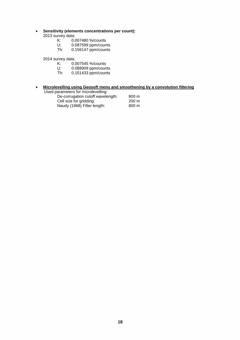
Sensitivity (elements concentrations per count): 2013 survey data:

K: 0.007480 %/counts U: 0.087599 ppm/counts Th: 0.156147 ppm/counts 2014 survey data:

K: 0.007545 %/counts U: 0.088909 ppm/counts Th: 0.151433 ppm/counts

Microlevelling using Geosoft menu and smoothening by a convolution filtering Used parameters for microlevelling:

De-corrugation cutoff wavelength: 800 m Cell size for gridding: 200 m Naudy (1968) Filter length: 800 m

19

Figure 4: Notodden survey area with flight path

20

Figure 5: Total Magnetic Field

21

Figure 6: Magnetic Vertical Derivative

22

Figure 7: Magnetic Tilt Derivative

23

Figure 8: Apparent resistivity. Frequency 6600 Hz, Coplanar coils

24

Figure 9: In-phase and quadrature response. Frequency 880 Hz, coplanar coils

25

Figure 10: Apparent resistivity. Frequency 7000 Hz, Coaxial coils

26

Figure 11: In-phase and quadrature response. Frequency 980 Hz, Coaxial coils

27

Figure 12: Uranium ground concentration

28

Figure 13: Thorium ground concentration

29

Figure 14: Potassium ground concentration

30

Figure 15: Radiometric Ternary map

Geological Survey of NorwayPO Box 6315, Sluppen7491 Trondheim, Norway

Visitor addressLeiv Eirikssons vei 39, 7040 Trondheim

Tel (+ 47) 73 90 40 00Fax (+ 47) 73 92 16 20E-mail ngu@ngu.no Web www.ngu.no/en-gb/

Norges geologiske undersøkelsePostboks 6315, Sluppen7491 Trondheim, Norge

BesøksadresseLeiv Eirikssons vei 39, 7040 Trondheim

Telefon 73 90 40 00Telefax 73 92 16 20E-post ngu@ngu.no Nettside www.ngu.no

NGUNorges geologiske undersøkelseGeological Survey of Norway