Proceedings of the 5th International Conference on Inverse Problems in Engineering: Theory and Practice,Cambridge, UK, 11-15th July 2005

NEW SET-MEMBERSHIP TECHNIQUES FOR PARAMETER ESTIMATION IN PRESENCE OFMODEL UNCERTAINTY

I. BRAEMS1, N. RAMDANI2, A. BOUDENNE2, L. JAULIN3, L. IBOS2, E. WALTER4 and Y. CANDAU2

1 LEMHE, UMR 8647, CNRS-Université Paris-Sud, Bt.410, 91405 Orsay, France.e-mail : isabelle.braems@lemhe.u-psud.fr2 CERTES, EA3481 Université Paris XII-Val-de-Marne, 61 avenue du Général de Gaulle, 94010 Créteil, Francee-mail : {ramdani, boudenne, ibos, candau}@univ-paris12.fr3 E3I2, ENSIETA 2, rue François Verny 29806 Brest, Cedex 9e-mail : jaulinlu@ensieta.fr4 L2S, UMR 8506, CNRS-Supélec-Université Paris XI, 91192 Gif-sur-Yvette, Francee-mail : eric.walter@lss.supelec.fr

Abstract – This paper introduces new methods for estimating parameters and their uncertainty in the contextof inverse problems. The new techniques are capable of dealing with both measurement and modelling errors butalso with uncertainty in parameters of the model that are assumed known. All the uncertain quantities are takenas unknown but bounded. In such a bounded-error context, reliable set-membership techniques are used tocharacterize, in a guaranteed way, the set of the unknown physical parameters that are compatible with thecollected experimental data, the model and the prior error bounds. This ensures that no solution is lost. Themethodology described will be applied to the simultaneous identification of thermal conductivity and diffusivityof polymer materials by a periodic method from actual experimental data. The guaranteed approaches provide anatural description of the uncertainty associated with the identified parameters.

1 INTRODUCTIONThis paper introduces new methods for estimating parameters and their uncertainty in the context of inverseproblems. These methods are capable of dealing not only with both measurement and modelling errors but alsowith uncertainty in parameters of the model that are not to be estimated (nuisance parameters).

The parameter estimation problem is usually solved with the widespread least-square approach, whichminimizes an eventually weighted quadratic norm of the difference between the vector of collected data and themodel output. Because the models employed are often nonlinear with regard to the unknown parameters, thisminimization is most often performed by local iterative search algorithms such as the Newton, Gauss-Newton,Levenberg-Marquardt, quasi-Newton or conjugate gradients technique [1], even though it is common knowledgethat the resulting estimate is very sensitive to initialization. Indeed, the search method may get trapped near alocal minimum or stop before reaching the actual global minimum. Alternative global optimization techniquesbased on random search may partly overcome this problem, but again the results are obtained with no guarantee.

Moreover, the measurement of physical parameters by identification should be regarded in a same way asany experimental measurement technique, which means that an uncertainty region for the estimated parametersshould always be provided. The Cramèr-Rao bound, given by the inverse of the Fisher information matrix, iscommonly used to quantify this uncertainty. It corresponds to the asymptotic variance of the maximum-likelihood estimate under the hypothesis that the data are corrupted by a noise with known probabilisticdistribution and that the knowledge model is valid [1]. Unfortunately, the number of collected experimental datamight be small, the measurement uncertainty may be partly due to some deterministic systematic errors, nocredible probability distribution may be available for the noise, and the knowledge models are most often basedon some important simplifying hypotheses (such that those about radiative or convective heat fluxes, forinstance). It is therefore more natural to assume all the uncertain quantities as unknown but bounded. In such abounded-error context, the solution is no longer a point but is the set of all acceptable values of the parametervector, which render model output consistent with actual data and prior error bounds.

The first aim of this paper is to introduce this new approach, known as bounded-error estimation, or setmembership estimation (see e.g. [2-6] and references therein) which characterizes the set of all acceptable valuesof the parameter vector. The size of this set quantifies naturally the uncertainty associated with the estimatedparameters. Moreover, as all the acceptable values of the parameter vector are enclosed, this approach allows theprior identifiability study, i.e. the issue of identified parameters unicity, to be bypassed and potentiallyunidentifiable parameters to be estimated. This relatively new technique has been developed in the fields ofcontrol and signal processing and has been recently used in electrochemistry [7] and robot localization [8]. It hasbeen investigated for the first time by the authors for a guaranteed characterization of a thermal experimental set-up [9-11].

The second aim of this paper is to deal with the fact that the knowledge-based model involves other uncertainparameters than those to be estimated. Usually, these parameters, to be called nuisance parameters from now on,are assumed to be known. In fact, they are subject to uncertainty corresponding to imprecise measurement,insufficient knowledge or strong modelling simplification. Obviously, this uncertainty can be expected to affectboth the identified parameters and their uncertainty. In order to take into account this disturbance, Fadale [12]has proposed an extended maximum-likelihood estimator in which the above nuisance parameters are modelledas normal random variables with known variance. The uncertainty associated which the identified parameters isthen derived from the asymptotic variance of the estimator. The use of the asymptotic variance with fewexperimental data has already been criticized above. In addition, the prior distribution of the nuisance parametersis not always known, except for the optimistic case where they are actually measured in repeated experiments. Inthe general case, only a range of values is available. Last, characterizing uncertainty by random variables maynot be a valid approach as modelling error may induce systematic errors which cannot be taken into account bystochastic variables. Consequently, the uncertainty in the nuisance parameters will be also characterized byintervals in the following. We shall show that set-membership estimation can reliably account for this type ofuncertainty.

Section 2 details the framework of bounded-error set estimation. Section 3 introduces interval analysis andconstraint propagation techniques, which allow the set estimation algorithms presented in section 4 to be reliable.The method is illustrated in section 5 with the simultaneous estimation of thermal conductivity and diffusivity ofa polymeric sample material via a periodic method and actual experimental data.

2. SET-MEMBERSHIP ESTIMATIONIn the sequel two types of parameters will be distinguished. The parameters of interest, i.e., those to beidentified, are in the parameter vector p. The other non-essential parameters are gathered in a vector q called thenuisance parameter vector. It is assumed that pŒP and qŒQ ,where P and Q are known prior domains.

Let e be the model output error e = y – f(p,q), where y is the vector of the collected data and f(.,.) thecorresponding model output. In bounded-error estimation (or set-membership estimation), one looks for the setof all parameter vectors such that the error stays within some known feasible domain E, i.e., eŒE (see [4-5] andthe references therein). The set estimate then contains all values of the parameter vector that are acceptable, i.e.,consistent with the model and the collected data y, given what is deemed an acceptable error. The size of this setquantifies the uncertainty associated with the estimated parameters.

Assume first that the value q* taken by the nuisance parameter vector q is known. The set C to be estimatedis the set of all the acceptable parameter vectors p

( ){ }, , *= ∈ ∈C P Yp f p q (1)

where Y = y + E. Characterizing C is a set-inversion problem, as (1) can be rewritten as( )1−

= ∩C Y Pg (2)where g(.) = f(.,q*). It can be solved in a guaranteed way using the algorithm SIVIA [13-15], see Section 3.

Suppose now that q* is unknown. One may of course choose to estimate the set( ) ( ){ }, | ,= ∈ × ∈S P Q Yp q f p q (3)

which can again be seen as a set-inversion problem. However, characterizing S will be much more difficult thanestimating C, since the dimension of S is larger than that of C and the volume of S may be very large, if theparameters in (p, q) are not identifiable.

Since the value of q is not considered essential, an alternative simpler approach is to characterize the set Π ofall the acceptable parameter vectors p under the assumption that q belongs to its prior domain, i.e.,

( ){ }| , ,Π = ∈ ∃ ∈ ∈P Q Yp q f p q (4)

The estimation of the acceptable values of q is then given up to simplify computation. While C is a cut of S,Π is the projection of S onto the p-space (see Figure 1)

Π =PSproj (5)

Remark 1. The inclusion C Ã Π, illustrates the fact that when q is uncertain, the uncertainty on p increases.

The basic tools for the characterization of Π will now be presented.

p1

S

p2

q

P

�

q*

C

Q

Figure 1 : The sets to be characterized

3. INTERVAL ANALYSISInterval analysis was initially developed to account for the quantification errors introduced by the rationalrepresentation of real numbers with computers and was extended to validated numerics [15-16-17]. A realinterval ,a a a[ ] = [ ] is a connected and closed subset of R. The set of all real intervals of R is denoted by IR.

Real arithmetic operations are extended to intervals [16]. Consider an operator ∑ Œ {+ , - , * , § } and [a] and [a]two intervals, then

[ ] [ ] [ ] [ ]{ },= ∈ ∈� �a b x y x a y b (6)

Let : →R Rn mf , the range of the function f over an interval vector [a] is given by:

[ ]( ) ( ) [ ]{ }| ∈f a f x x a��� (7)

The interval function [f] from IRn to IRm is an inclusion function for f if[ ] [ ]( ) [ ] [ ]( ),∀ ∈ ⊆IR

na f a f a (8)

An inclusion function of f can be obtained by replacing each occurrence of a real variable by its correspondinginterval and by replacing each standard function by its interval evaluation. Such a function is called the naturalinclusion function. In practice the inclusion function is not unique, it depends on how f is written.

For the sake of brevity, the same notation will be used for the ranges of the used functions and their inclusionfunctions.

Constraints satisfaction problem, contractorsConsider n variables xi ∈ R, i ∈ {1,2,…,n}, linked by nf relations of the form

1 2( , , , ) 0=…j nf x x x (9)and where each variable xi is known to belong to a prior interval domain [xi]0 ; define the vector

T1 2 = ( , , , )… nx x xx and the function T

1 2 = ( , , , )…

fnf f ff x x x x( ) ( ) ( ) ( ) , then equation (9) can be written as aconstraint satisfaction problem CSP [15] :

H : = , ∈f x 0 x x 0( ) [ ] (10)Interval CSPs can be solved with contractors. An operator CH is a contractor for the CSP H defined by (10)

if, for any box [x] in [x]0, it satisfiesa) the contractance property : [ ]( ) [ ]⊂HC x x

b) and the correctness property : [ ]( ) [ ]∩ = ∩HC x xS S

where ∩ is the intersection of two boxes and S a solution set for H. A solver for the CSP defined by (10) is analgorithm Ψ such that:

( ) ( )= ⇔ = Ψf x 0 x x (11)According to the fixed-point theorem and using (11), if the series 1 ( )

+= Ψk kx x converges towards

∞x , then

∞x shall contain the solution of H. Several punctual solvers such as the Newton method, the Gauss-Siedel or theKrawczyk operators have been extended to intervals, and are used to solve efficiently even non-linear CSPs [15-17]. However, they remain limited to problems where the number of constraints is equal to the number ofvariables.

When the number of constraints and the number of variables are different, one can use an alternate contractorrelying on interval propagation techniques. These techniques combine the constraint propagation techniquesclassically used in the domain of artificial intelligence [18] and interval analysis. They have been brought toautomatic control in [19], for solving set inversion problems in a bounded-error context. The algorithm used forconstraint propagation is based on the interval extension of the local Waltz filtering [18-19]. In fact, therelationships (9) between the variables can be viewed as a network where the nodes are connected with theconstraints. In order to spread the consequences of each node throughout the network, the main idea is to dealwith a local group of constraints and nodes and then record the changes in the network. Further deductions willmake use of these changes to make further changes. The inconsistent values for the state vector are thusremoved. If the network exhibits no cycles, then optimal filtering can be achieved by performing only oneforward and one backward propagation: this is known as the forward-backward contractor [15-19]. Figure 2illustrates several types of contractors.

CC([ ])p

[ ]p

CC([ ])p

[ ]p

CeC([ ])p

[ ]p

CeC([ ])p

[ ]p

C

Figure 2 : Contractors.

Set inversion via interval analysisConsider the problem of determining a solution set for the unknown quantities u defined by:

( ) [ ]{ } [ ]( )1| −

= ∈ Ψ ∈ = Ψ ∩u u y yS U U (12)

where [ ]y is known a priori, U is an a priori search set for u and ψψψψ a nonlinear function not necessarilyinvertible in the classical sense. Equation (12) involves computing the reciprocal image of ΨΨΨΨ, it is a set inversionproblem which can be solved using SIVIA (Set Inversion Via Interval Analysis). SIVIA [13-14] is a recursivealgorithm which explores all the search space without losing any solution. This algorithm makes it possible toderive a guaranteed enclosure of the solution set S as follows

⊆ ⊆S S S (13)The inner enclosure S is composed of the boxes that have been proved feasible. To prove that a box [u] is

feasible it is sufficient to prove that Ψ ⊆u y([ ]) [ ] . Contrariwise, if it can be proved that Ψ ∩ =∅u y([ ]) [ ] , thenthe box [u] is unfeasible. Otherwise, no conclusion can be reached and the box [u] is said undetermined. Thelatter is then bisected and tested again until its size reaches a threshold ε > 0 to be tuned by the user. Such atermination criterion ensures that SIVIA terminates after a finite number of iterations. The outer enclosure S isdefined by

= ∪∆S S S (14)where ∆S is an uncertainty layer given by the union of all the undetermined boxes (with their widths not largerthan ε ).

Set projection via interval analysisWhen only Π is to be characterized, one can use another algorithm called PROJECT [9,10,11,19]. Thisalgorithm computes inner and outer approximations Π and Π of the set Π defined by (4). As only the p-spaceis partitioned, the memory and computational time required are much smaller than for a full characterization ofS. Obviously, the main difference between PROJECT and SIVIA lies in the tests to be implemented. In SIVIA,the outer approximation [g]([p]) is directly used to test the acceptability of all elements of [p]. Here, tocharacterize Π , [p] will be said acceptable if there exists q∈Q such that f([p],q)⊂Y. Feasible point finders thenrequire specific approaches. In order to allow consideration of higher dimensions, the procedure implemented inPROJECT uses contractors (see [19] for details). As only the p-space is partitioned, the memory andcomputational time required are much smaller than for a full characterization of S.

4. APPLICATION

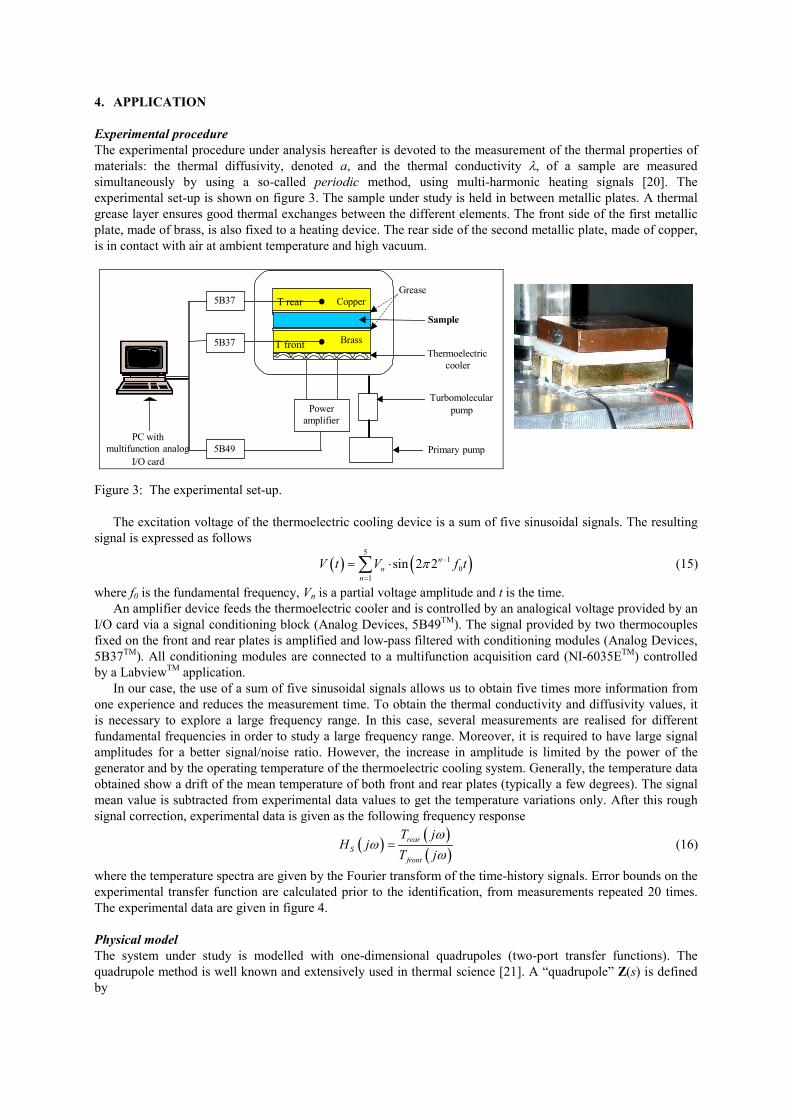
Experimental procedureThe experimental procedure under analysis hereafter is devoted to the measurement of the thermal properties ofmaterials: the thermal diffusivity, denoted a, and the thermal conductivity λ, of a sample are measuredsimultaneously by using a so-called periodic method, using multi-harmonic heating signals [20]. Theexperimental set-up is shown on figure 3. The sample under study is held in between metallic plates. A thermalgrease layer ensures good thermal exchanges between the different elements. The front side of the first metallicplate, made of brass, is also fixed to a heating device. The rear side of the second metallic plate, made of copper,is in contact with air at ambient temperature and high vacuum.

5B37

5B37

Poweramplifier

5B49

Turbomolecularpump

Primary pumpPC with

multifunction analogI/O card

Copper

Sample

BrassThermoelectric

cooler

Grease

Figure 3: The experimental set-up.

The excitation voltage of the thermoelectric cooling device is a sum of five sinusoidal signals. The resultingsignal is expressed as follows

( ) ( )5

10

1sin 2 2π

−

=

= ⋅∑n

nn

V t V f t (15)

where f0 is the fundamental frequency, Vn is a partial voltage amplitude and t is the time.An amplifier device feeds the thermoelectric cooler and is controlled by an analogical voltage provided by an

I/O card via a signal conditioning block (Analog Devices, 5B49TM). The signal provided by two thermocouplesfixed on the front and rear plates is amplified and low-pass filtered with conditioning modules (Analog Devices,5B37TM). All conditioning modules are connected to a multifunction acquisition card (NI-6035ETM) controlledby a LabviewTM application.

In our case, the use of a sum of five sinusoidal signals allows us to obtain five times more information fromone experience and reduces the measurement time. To obtain the thermal conductivity and diffusivity values, itis necessary to explore a large frequency range. In this case, several measurements are realised for differentfundamental frequencies in order to study a large frequency range. Moreover, it is required to have large signalamplitudes for a better signal/noise ratio. However, the increase in amplitude is limited by the power of thegenerator and by the operating temperature of the thermoelectric cooling system. Generally, the temperature dataobtained show a drift of the mean temperature of both front and rear plates (typically a few degrees). The signalmean value is subtracted from experimental data values to get the temperature variations only. After this roughsignal correction, experimental data is given as the following frequency response

( )( )

( )

ω

ω

ω

=

rearS

front

T jH j

T j(16)

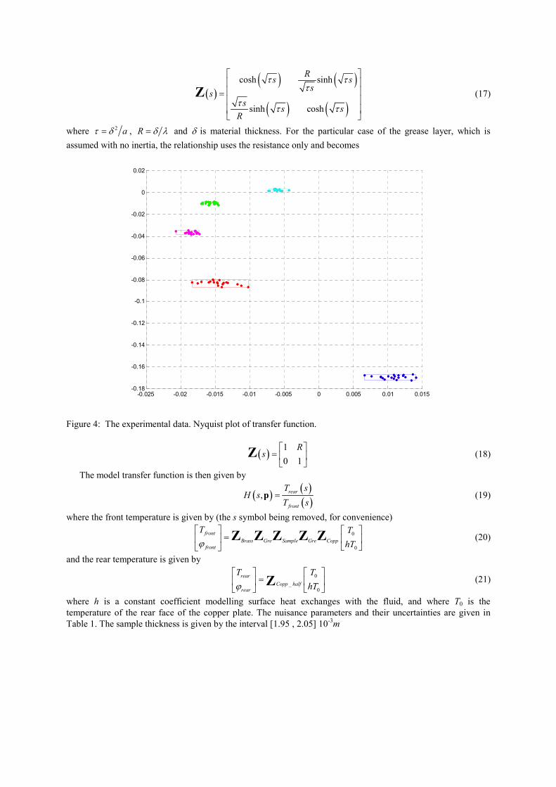
where the temperature spectra are given by the Fourier transform of the time-history signals. Error bounds on theexperimental transfer function are calculated prior to the identification, from measurements repeated 20 times.The experimental data are given in figure 4.

Physical modelThe system under study is modelled with one-dimensional quadrupoles (two-port transfer functions). Thequadrupole method is well known and extensively used in thermal science [21]. A “quadrupole” Z(s) is definedby

T rear

T front

( )( ) ( )

( ) ( )

cosh sinh

sinh cosh

τ τ

τ

τ

τ τ

=

Rs sss

s s sR

Z (17)

where 2τ δ= a , δ λ=R and δ is material thickness. For the particular case of the grease layer, which is

assumed with no inertia, the relationship uses the resistance only and becomes

-0.025 -0.02 -0.015 -0.01 -0.005 0 0.005 0.01 0.015-0.18

-0.16

-0.14

-0.12

-0.1

-0.08

-0.06

-0.04

-0.02

0

0.02

Figure 4: The experimental data. Nyquist plot of transfer function.

( )10 1

=

RsZ (18)

The model transfer function is then given by

( )( )

( ), =

rear

front

T sH s

T sp (19)

where the front temperature is given by (the s symbol being removed, for convenience)

0

0ϕ

=

frontBrass Gre Sample Gre Copp

front

T ThT

Z Z Z Z Z (20)

and the rear temperature is given by

0_

0ϕ

=

rearCopp half

rear

T ThTZ (21)

where h is a constant coefficient modelling surface heat exchanges with the fluid, and where T0 is thetemperature of the rear face of the copper plate. The nuisance parameters and their uncertainties are given inTable 1. The sample thickness is given by the interval [1.95 , 2.05] 10-3m

Material Parameters Scale Nominalvalue

Uncertaintyinterval

Diffusivity, a 10-6 m2.s-1 34.0 [33 , 35]Conductivity, λ W.m-1.K-1 112.5 [100 , 125]

Brass plateFront side

Brass thermocouple – sample interface distance 10-3 m 5.0 [4.225 , 5.775]Diffusivity, a 10-6 m2.s-1 115.5 [114 , 117]Conductivity, λ W.m-1.K-1 395.5 [389 , 402]Copper thermocouple – sample interface distance 10-3 m 4.5 [3.725 , 5.275]

Copper plateRear side

Thickness 10-3 m 9.0 [8.89 , 9.01]Grease Thermal resistance 10-6 K.m2.W-1 115.0 [80 , 150]Fluid Surface heat exchange coefficient W.m-2.K-1 5 [5 , 10]

Table 1: Nuisance model parameters..5. RESULTS

In this section, two cases are studied. First, the parameters are estimated while assuming the nuisance parametersperfectly known, then the latter are assumed uncertain. In both cases, the prior search space for the parameters istaken as:

[ ]1, 30τ ∈p s1/2 and 410 , 5− ∈ pR m2.K.W-1 (22)

Bounded-error identification with set inversion, nuisance parameters assumed knownSIVIA with a contractor, ε = 0.001 derives in 2 s the inner and outer approximations plotted in figure 5. Theprojection of the outer approximation C onto the parameter axes provides an outer approximation of theuncertainty associated with each of the identified parameters

88.167 10 8.3%−

= ⋅ ±a m2.s-1 (23)and 0.201 4.6%λ = ± W.m-1.K-1 (24)

Figure 5: Inner (dark boxes) and outer approximation of posterior feasible set C.(Light grey boxes are the uncertainty layer ∆C)

Compare (23)-(24) with the estimated parameters given by least square estimation, i.e.88.767 10 1.9%−

= ⋅ ±a m2.s-1 (25)and 0.179 0.4%λ = ± W.m-1.K-1 (26)

The reader can see that the estimated uncertainty in the identified parameters is much smaller for leastsquares results. Still, the value identified for the diffusivity parameter a with set inversion is consistent with theone given by least squares.

Rp ( m2KW-1)

( )12

p sτ

However, the values identified for the conductivity parameter λ with both methods are significantlydifferent. In order to explain this result, we have checked both identified models outputs: we found that theoutput of the model identified with least squares is not included in the prior bounds for experimental data at thelowest frequency, which is possible because this was not the purpose of least squares estimation. At thecontrary, the output of the model given by set inversion is indeed included in the prior bounds for experimentaldata as this was the purpose of the bounded error estimation technique.

Bounded-error identification with set projection, nuisance parameters assumed uncertainNow assume the nuisance parameters are uncertain, PROJECT derives in 300s the inner and outerapproximations plotted in figure 6. The large thickness of the uncertainty layer is due to the pessimism of thecontractors and inclusion functions employed, which limits the quality of the results.

The projection of the outer approximation Π onto the parameter axes provides an outer approximation of theuncertainty associated with each of the identified parameters

88.13 10 22%−

= ⋅ ±a m2.s-1 (27)and 0.205 15%λ = ± W.m-1.K-1 (28)

As expected, the uncertainty in the nuisance parameters leads to much larger uncertainties in the identifiedparameters.

Figure 6: Inner (dark boxes) and outer approximation of posterior feasible set Π.(Light grey boxes are the uncertainty layer ∆Π).

CONCLUSIONIn this paper we have addressed the problem of reliable parameter estimation in presence of model uncertaintyresulting from nuisance parameters.

In the first part of this paper, we assumed that the nuisance parameter vector was accurately known.Assuming that the errors on model output were bounded but otherwise unknown, we have showed thatestimating the parameters in such a framework is a set inversion problem. The algorithm SIVIA has been usedwith data taken from an actual experimental thermal set-up. The new method generates inner and outerapproximations for the solution set which provides a simple evaluation of the estimation uncertainty.

In the second part of this paper, we have addressed the problem of estimating the feasible parameter set whenthe nuisance parameter are uncertain. We have shown that estimating the parameters in this framework amounts

Rp ( m2KW-1)

12

p sτ

to projecting the solution set onto the space of the parameters of interest. We characterized this projection withthe algorithm PROJECT. The volume of this projected set is larger than the one derived when the nuisanceparameters are assumed accurately known: taking into account uncertainty increases the uncertainty associatedwith the estimation. One is now capable of accounting for bounded uncertainty in nuisance parameters in areliable and guaranteed way.

REFERENCES

1. P. Eykhoff, System Identification, John Wiley And Sons, 1979.

2. M. Milanese, J. Norton, H. Piet-Lahanier, and E. Walter, editors. Bounding Approaches to SystemIdentification. Plenum Press, New York, NY, 1996.

3. G. Belforte, B. Bona, and V. Cerone, Parameter estimation algorithms for a set-membership description ofuncertainty, Automatica, 26(5):887-898, 1990.

4. J. P. Norton, editor, Special Issue on Bounded-Error Estimation: Issue 2. 1995, International Journal ofAdaptive Control and Signal Processing 9(1):1-132.

5. M. Milanese and A. Vicino, Estimation theory for nonlinear models and set membership uncertainty,Automatica, 27(2):403-408, 1991.

6. E. Walter, editor. Special Issue on Parameter Identification with Error Bounds, 1990, Mathematics andComputers in Simulation 32(5-6):447-607.

7. I. Braems, F. Berthier, L. Jaulin, M. Kieffer, and E. Walter. Guaranteed estimation of electrochemicalparameters by setinversion using interval analysis, Journal of Electroanalytical Chemistry, 495(1):1-9,2001.

8. M. Kiffer, L. Jaulin, E. Walter, and D. Meizel, Robust autonomous robot localization using intervalanalysis, Reliable Computing, 6(3):337-362, 2000.

9. I. Braems, Méthodes ensemblistes garanties pour l'estimation de grandeurs physiques, PhD dissertation,Université Paris-Sud, Orsay, France, 2002.

10. I. Braems, N.Ramdani, M. Kieffer & E. Walter, Caractérisation garantie d'un dispositif de mesure degrandeurs thermiques, APII-Journal Européen des Systèmes Automatisés, 37(9) :1129-1143, 2003.

11. I.Braems, L.Jaulin, M.Keiffer, N.Ramdani & E.Walter, Reliable parameter Estimation in Presence ofUncerainty, 13th IFAC Symposium on System Identification, Rotterdam, SYSID 2003, pp.1856-1861.

12. T.D. Fadale, A.V. Nenarokomov, and A.F. Emery, Uncertainties in parameter estimation: The inverseproblem, The International Journal of Heat and Mass Transfer, 38(3):511-518, 1995.

13. L. Jaulin and E. Walter, Guaranteed nonlinear parameter estimation from bounded-error data via intervalanalysis. Mathematics and Computers in Simulation, 35(2):123-137, 1993.

14. L. Jaulin and E. Walter, Set inversion via interval analysis for nonlinear bounded-error estimation,Automatica, 29(4):1053-1064, 1993.

15. L. Jaulin, M. Kieffer, O. Didrit, and E. Walter, Applied Interval Analysis, Springer-Verlag, London, 2001.

16. R. E. Moore, Interval Analysis, Prentice-Hall, Englewood Cliffs, NJ, 1966.

17. A. Neumaier, Interval methods for systems of equations, Cambridge University Press, Cambridge, 1990.

18. E. Davis, Constraint propagation with interval labels, Artificial Intelligence (32), 1987, 281-331.

19. L. Jaulin, I. Braems, and E. Walter, Interval methods for nonlinear identification and robust control, In41st IEEE Conference on Decision and Control, pages 4676-4681, Las Vegas, 2002.

20. A. Boudenne, L. Ibos, E. Gebin, and Y. Candau, A simultaneous characterization of thermal conductivityand diffusivity of polymer materials by a periodic method, Journal of Physics D: Applied Physics, 37:132-139, 2004.

21. H. Wang, A. Degiovanni, and C. Moyne, Periodic thermal contact: a quadrupole model and an experiment,International Journal of Thermal Science, 41:125-135, 2002.