new sensorless, efficient optimized and stabilized v/f
TRANSCRIPT

Scholars' Mine Scholars' Mine
Masters Theses Student Theses and Dissertations
Fall 2013
New sensorless, efficient optimized and stabilized V/f control for New sensorless, efficient optimized and stabilized V/f control for
PMSM machines PMSM machines
Seyed Hesam Jafari
Follow this and additional works at: https://scholarsmine.mst.edu/masters_theses
Part of the Electrical and Computer Engineering Commons
Department: Department:
Recommended Citation Recommended Citation Jafari, Seyed Hesam, "New sensorless, efficient optimized and stabilized V/f control for PMSM machines" (2013). Masters Theses. 5439. https://scholarsmine.mst.edu/masters_theses/5439
This thesis is brought to you by Scholars' Mine, a service of the Missouri S&T Library and Learning Resources. This work is protected by U. S. Copyright Law. Unauthorized use including reproduction for redistribution requires the permission of the copyright holder. For more information, please contact [email protected].


NEW SENSORLESS, EFFICIENT OPTIMIZED AND STABILIZED V/F CONTROL FOR PMSM MACHINES
by
SEYED HESAM JAFARI
A THESIS
Presented to the Faculty of the Graduate School of the
MISSOURI UNIVERSITY OF SCIENCE AND TECHNOLOGY
In Partial Fulfillment of the Requirements for the Degree
MASTER OF SCIENCE IN ELECTRICAL ENGINEERING
2013
Approved by
Dr. Jonathan Kimball, Advisor Dr. Keith Corzine, Co Advisor
Dr. Mehdi Ferdowsi

2013
Seyed Hesam Jafari
All Rights Reserved

iii
ABSTRACT
With the rapid advances in power electronics and motor drive technologies in
recent decades, permanent magnet synchronous machines (PMSM) have found extensive
applications in a variety of industrial systems due to its many desirable features such as
high power density, high efficiency, and high torque to current ratio, low noise, and
robustness. In low dynamic applications like pumps, fans and compressors where the
motor speed is nearly constant, usage of a simple control algorithm that can be
implemented with least number of the costly external hardware can be highly desirable
for industry.
In recent published works, for low power PMSMs, a new sensorless volts-per-
hertz (V/f) controlling method has been proposed which can be used for PMSM drive
applications where the motor speed is constant. Moreover, to minimize the cost of motor
implementation, the expensive rotor damper winding was eliminated. By removing the
damper winding, however, instability problems normally occur inside of the motor which
in some cases can be harmful for a PMSM drive. As a result, to address the instability
issue, a stabilizing loop was developed and added to the conventional V/f.
By further studying the proposed sensorless stabilized V/f, and calculating power
loss, it became known that overall motor efficiency still is needed to be improved and
optimized. This thesis suggests a new V/f control method for PMSMs, where both
efficiency and stability problems are addressed. Also, although in nearly all recent related
research, methods have been applied to low power PMSM, for the first time, in this
thesis, the suggested method is implemented for a medium power 15 kW PMSM.
A C2000 F2833x Digital Signal Processor (DSP) is used as controller part for the
student custom built PMSM drive, but instead of programming the DSP in Assembly or
C, the main control algorithm was developed in a rapid prototype software environment
which here Matlab Simulink embedded code library is used.

iv
ACKNOWLEDGMENTS
First and foremost I would like to say thanks to my advisors Dr. Jonathan Kimball
and Dr. Keith Corzine for their time, patience, and dedication to my higher learning. I
highly appreciate them trusting me and utilizing their vast knowledge of electrical
engineering to aid in my advancement of becoming a better researcher and a professional
engineer prepared to work in industry.
I should also say thanks to my thesis committee Dr. Mehdi Ferdowsi for the
valuable advice he gave to me through these last years. Here, at MST I took nearly all my
courses with my thesis committee members where they helped me to increase my
knowledge and develop a solid background in the area of power electronic, electrical
vehicle and motor drive.
This work was supported by the Department of Energy under contract DE-
EE0002012.
Next, I would like to thank God that gave me enough power to write this thesis
and then my parents for their support and direction through my journey of this master’s
program. I owe them all of my life successes and accomplishments and always thankful
to them because they sacrificed their life for me and my sister.

v
TABLE OF CONTENTS
Page
ABSTRACT ....................................................................................................................... iii
ACKNOWLEDGMENTS ................................................................................................. iv
LIST OF ILLUSTRATIONS ............................................................................................ vii
LIST OF TABLES .............................................................................................................. x
NOMENCLATURE .......................................................................................................... xi
SECTION
1. INTRODUCTION ...................................................................................................... 1
1.1. MOTIVATION ................................................................................................... 1
1.2. PERMANENT MAGNET SYNCHRONOUS MACHINES (PMSM) .............. 1
2. CONTROL METHOD ............................................................................................... 4
2.1. REVIEW OF THE SENSORLESS CONTROLLING METHOD OF PMSM .. 4
2.2. VOLTAGE CONTROL METHOD AND STABILITY ANALYSIS ................ 5
2.3. STABILITY ANALYSIS ................................................................................... 8
2.4. FREQUENCY MODULATION TECHNIQUE ............................................... 12
2.5. EFFICIENCY OPTIMIZATION OF THE STABILIZED V/F CONTROL .... 14
3. DSP IMPLEMENTATION USING MATLAB/SIMULINK .................................. 17
3.1. INTRODUCTION ............................................................................................ 17
3.2. TOP LEVEL ..................................................................................................... 18
3.3. ADC UNIT AND SUBSYSTEM ..................................................................... 23
3.4. MAIN PROGRAM SUBSYSTEM................................................................... 25
3.5. EPWM UNIT .................................................................................................... 30
3.6. ECAN UNIT ..................................................................................................... 35
3.6.1. Basics.. .................................................................................................... 36
3.6.2. Message Frame Architecture.. ................................................................ 38
3.6.3. Message Broadcasting and Error Detection... ........................................ 40
3.6.4. Canoe Software… .................................................................................. 41
3.6.5. Can Using Simulink’s Embedded Coder.. .............................................. 42
4. SIMULATION AND EXPERIMENTAL RESULTS ............................................. 47

vi
4.1. SIMULATION .................................................................................................. 47
4.2. EXPERIMENTAL RESULTS.......................................................................... 54
4.3. ISSUES ENCOUNTERED DURING THE IMPLEMENTATION................. 60
4.3.1. Software Issue. . .................................................................................... 60
4.3.2. Debugging. ............................................................................................. 61
5. CONCLUSIONS ...................................................................................................... 63
BIBLIOGRAPHY ............................................................................................................. 64
VITA. ……………………………………………………………………………………66

vii
LIST OF ILLUSTRATIONS
Page
Figure 1.1. Diagram of conceptual drive system ................................................................ 2
Figure 1.2. Two poles salient PMSM ................................................................................. 3
Figure 2.1. Steady-state vector diagram of the PMSM in synchronized reference frame .. 6 Figure 2.2. Calculation of the voltage command ................................................................ 8
Figure 2.3. Primary drive configuration with V/f control method ...................................... 8
Figure 2.4. Loci of the rotor poles under different load conditions, as a function of the applied frequency ........................................................................................... 11
Figure 2.5. Measured rotor speeds at different frequencies, under no load ...................... 13
Figure 2.6. Derivation of the frequency modulation signal 𝛥𝑤𝑃 ..................................... 14
Figure 2.7. Vector diagram of PMSM with maximum torque per amp ............................ 15
Figure 2.8. Final control diagram for PMSM after adding the stabilized and efficiency loop to the preliminary configuration .......................................................... 16
Figure 3.1. The top level in the implementation of DSP program in the Matlab/ Simulink, left window, and the properties of the Hardware Interrupt block, right window .................................................................................................. 19
Figure 3.2. Target Preferences block can be fine in Simulink Library Embedded Coder >> Embed Targets ......................................................................................... 20
Figure 3.3. Configuration Parameters (simulation tab in Simulink) ................................. 21
Figure 3.4. Interrupt vector table ...................................................................................... 23
Figure 3.5. ADC subsystem implementing measurement and scaling ............................. 24
Figure 3.6. Unit delay implementation using 6 unit delay blocks .................................... 25
Figure 3.7. Show the properties of the ADC module ....................................................... 25
Figure 3.8. Implementation of sensor less stabilized efficient V/f for PMSM drive in Main Program subsystem .............................................................................. 26
Figure 3.9. Calculating the electrical angle from the motor speed and program sampling time ................................................................................................. 27
Figure 3.10. Finding voltage magnitude from frequency and a-b phases current ............ 28
Figure 3.11. Park transformation ...................................................................................... 29
Figure 3.12. Stabilization loop implementation ................................................................ 29
Figure 3.13. Efficiency loop implementation ................................................................... 30
Figure 3.14. Display of ePWM unit inside of the main program ..................................... 31

viii
Figure 3.15. Property panels of ePWM unit ..................................................................... 32
Figure 3.16. Property panels of ePWM unit ..................................................................... 33
Figure 3.17. A typical configuration to drive a 3-phase system consist of a DC bus and 3- phase full bridge ................................................................................. 34
Figure 3.18. Dead-band waveforms for typical cases ....................................................... 35
Figure 3.19. Comparison between older multi-wire setup and typical Can bus set up .... 37
Figure 3.20. CAN node example ...................................................................................... 38
Figure 3.21. CAN data frame for 29-Bit extended format ................................................ 39
Figure 3.22. CANoe configuration window ..................................................................... 42
Figure 3.23. CAN A preferences ...................................................................................... 43
Figure 3.24. Vector CAN box ........................................................................................... 44
Figure 3.25. D-sub pin out ................................................................................................ 44
Figure 3.26. CAN Pack Block .......................................................................................... 45
Figure 3.27. eCAN Transmit block .................................................................................. 46
Figure 4.1. Measured rotor speeds at different frequencies, under no load, without stabilizing loop in the system ........................................................................ 48
Figure 4.2. Measured rotor speeds at different frequencies, under no load, with stabilizing loop in the system ........................................................................ 49
Figure 4.3. Comparison of input real power ..................................................................... 51
Figure 4.4. Comparison of input reactive power .............................................................. 51
Figure 4.5. Comparison of stator voltage magnitude ........................................................ 52
Figure 4.6. Comparison of stator current magnitude ........................................................ 52
Figure 4.7. Comparison of stator current q component .................................................... 53
Figure 4.8. Comparison of stator current d component .................................................... 53
Figure 4.9. Comparison of rotor mechanical speed .......................................................... 54
Figure 4.10. Lab set up for efficient and stabilized V/f for PMSM machine ................... 55
Figure 4.11. Comparison of input real power. .................................................................. 56
Figure 4.12. Comparison of input reactive power. ........................................................... 56
Figure 4.13. Comparison of stator current magnitude. ..................................................... 57
Figure 4.14. Comparison of stator voltage magnitude. ..................................................... 57
Figure 4.15. Comparison of stator current q component. ................................................. 58
Figure 4.16. Comparison of stator current d component. ................................................. 58
Figure 4.17. Comparison of rotor mechanical speed. ....................................................... 59

ix
Figure 4.18. Comparison of applied load torque. ............................................................. 59

x
LIST OF TABLES Page
Table 2.1. PMSM motor parameters which its loci plot is shown in Figure 1.6 ………11
Table 2.2. PMSM motor parameters which were used in experimental tests….……... 47

xi
NOMENCLATURE
Symbol Description
l Length of the Conductor
F Exerted Force
B Magnetic Field
ϕ0 Power Factor Angle
Is Magnitude of the Current
Es Magnitude of the Voltage Vector
rs Stator Winding Resistance
λm Rotor Permanent-Magnet Flux
fo Applied frequency
ωe Electrical Speed
Bm Viscous Friction Coefficient
Vs Stator Voltage Magnitude
J Inertia of the Motor and the Load System
Vrated Rated Voltage Phase to Phase
Tlrated Load Torque
n Number of Poles of the Motor
iqsr Rotor q Axes Current
idsr Rotor d Axes Current
L Motor Inductance
vdc DC Power Supply
d Modulation Index
CAN Communication Area Network
PMSM Permanent Magnet Synchronized Motor
ADC Analog to Digital Converter
DSP Digital Signal Processor

1. INTRODUCTION
1.1. MOTIVATION
When PMSM drives are used for applications like pumps and fans, where high
dynamic performance is not a demand, a simple control strategy can be used instead of
the sensorless field-oriented- control approach that is heavily dependent on the rotor
position sensor. Furthermore, the PMSM damper windings in the rotor assure the
synchronization of motion of the rotor with the stator applied frequency, which is the
fundamental requirement for synchronous machine control. This allows a stable control
of this type of PMSM in an open-loop manner. However, due to the high manufacturing
cost and the difficulty to design rotors with damper windings for some type of PMSMs
the PMSMs are not generally available with damper windings in the rotor. The PMSMs
without damper windings in the rotor do not assure the synchronization of motion of the
rotor with stator applied frequency under the open-loop control approach. This causes
instability problems in those PMSMs under the open-loop control approach and an
additional signal is required to the controller in order to assure the synchronization and
the stable operation. Moreover, a PMSM using a damper winding may not have stability
issue but its functionality and operations may not be efficient and acceptable. Further
study shows that only 𝑚𝑞 stator current can contribute in effective torque generation
while 𝑚𝑑 stator current can increase the overall motor loss therefore the efficiency issue
needs to be addressed for any PMSM.
1.2. PERMANENT MAGNET SYNCHRONOUS MACHINES (PMSM)
The permanent-magnet synchronous machine (PMSM) drive has emerged as a top
competitor for a full range of motion control applications [1, 2, 3]. For example, the
PMSM is widely used in machine tools, robotics, actuators, and is being considered in
high-power applications such as vehicular propulsion and industrial drives. It is also
becoming viable for commercial/residential applications. The PMSM is known for
having high efficiency, low torque ripple, superior dynamic performance, and high power
density.

These drives often are the best choice for high-performance applications and are
expected to see expanded use as manufacturing costs decrease. The PMSM is a
synchronous machine in the sense that it has a multiphase stator and the stator electrical
frequency is directly proportional to the rotor speed in the steady state. However, it
differs from a traditional synchronous machine in that it has permanent magnets in place
of the field winding and otherwise has no rotor conductors. The use of permanent
magnets in the rotor facilitates efficiency, eliminates the need for slip rings, and
eliminates the electrical rotor dynamics that complicate control (particularly vector
control). The permanent magnets have the drawback of adding significant capital cost to
the drive, although the long term cost can be less through improved efficiency. The
PMSM also has the drawback of requiring rotor position feedback by either direct means
or by a suitable estimation system. Since many other high performance drives utilize
position feedback, this is not necessarily a disadvantage. A conceptual drive system is
pictured in Figure 1.1. There, a speed, position, or torque command is input to the drive
system. The motion controller implements feedback control based on mechanical sensors
(or estimators). The controller generates commands for the electrical variables to obey.
The electrical control block converts its input commands into commands for the power
converter/modulator block and sometimes utilizes feedback of voltage or current. The
power converter block imposes the desired electrical signals onto the PMSM machine
with the connected load.
Figure 1.1. Diagram of conceptual drive system

3
As in all electrical motors, a PMSM has two principle parts, a moving part and a
stationary part which are called rotor and stator. The phase windings are found in the
stator and can be configured in different ways, for example as sinusoidal, trapezoidal or
the more common concentrated winding. There are usually three phase windings since
most PMSMs are three phase motors, thus each winding is excited by a different phase.
When a current runs through windings a force is exerted on the current due to the
magnetic field of the rotor. This phenomena is called the Lorentz force and is described
by equation
F = l⃗ ∙ ( I⃗ × B��⃗ ) (1)
Here F is the force exerted, 𝑃 is length of the conductor, 𝐼 is the current flowing in the
conductor and B is the external magnetic field present. The counter force to equation (1)
is that causes the rotation of the rotor and transform electrical energy to mechanical
energy.
In Figure 1.2 the cross section of a simplified PMSM with concentrated winding
is depicted. The three phase windings are presented by u, v, w respectively and the rotor
is modeled as a simple magnet bar, thus this motor has two poles. The max torque
generation can achieved when the current and the magnetic vectors field are orthogonal.
Therefore, the goal of any motor control algorithm should be to keep the current flowing
in the stator winding orthogonal to the magnetic field of the rotor.
Figure 1.2. Two poles salient PMSM

4
2. CONTROL METHOD
2.1. REVIEW OF THE SENSORLESS CONTROLLING METHOD OF PMSM
With the rapid advances in power electronics and motor drive technologies in
recent decades, permanent magnet synchronous machines (PMSM) have found extensive
applications in a variety of industrial systems due to their many desirable features such as
high power density, high efficiency, and high torque to current ratio, low noise, and
robustness. However, using a PMSM also is associated with some limitations. One major
drawback of the most commonly used PMSM drive systems is that the control algorithm
requires the knowledge of the rotor position or speed, which requires the usage of an
encoder or a resolver, increasing the final machine cost and decreasing system reliability.
The use of these rotational transducers escalates the complexity of the motor
construction, complicates the production process, and increases the final machine cost,
while at the same time decreases system reliability. Sensorless control for PMSM has
been a desired field of study of researchers in recent years, and a large number of
sensorless control methods have been proposed over the years [4, 5, 6, 7, 8, 9, 10].
Among those methods, some utilize the position dependence of the back electromotive
force (EMF), some rely on rotor saliency characteristics, and the injection of various
kinds of test signals is used in some of recent papers. In [9], the authors proposed a novel
modified back EMF observer for rotor speed estimation based on sliding mode observer
theory using Lyapunov stability criteria. In [10], the sensorless operation of PMSM was
extended to all four quadrants and at significantly low speed, by measuring the current
derivative during the zero voltage switching vectors. The majorities of those methods are
based on the involved algorithms, and are proposed for the high dynamic application.
However, for applications where high dynamic performance is not a demand, such as
pump and fan motor drive systems, an inexpensive, a simpler and more robust method is
often desired. Moreover, due to the high manufacturing cost and difficulty to design rotor
with damper winding for some type of PMSMs, the PMSMs are not generally available
with damper winding on the rotor. As a result, using the open-loop V/f control approach
causes some instability problems in the PMSM performance. In [11], Perera et al. address
the inherent instability issue associated with the open-loop V/f control for PMSM that do

5
not have damper windings in the rotor, and then proposed such a sensorless control
technique that was integrated into a V/f control method in order to resolve the mentioned
problem. By modulating the applied voltage frequency proportional to the perturbations
in the input power, the method achieved a stable control in a wide frequency range while
maintaining a constant stator flux linkage of the motor.
Further detailed study of the method proposed by Perera et al. revealed that
although the suggested stabilized sensorless control is very effective, the overall PMSM
drive control is not optimized. Especially, in certain operating conditions, the non-
optimal choice of the stator flux linkage can lead to low motor efficiency. In this thesis,
an efficiency improvement method is proposed that can be combined with the sensorless
stable control in [11] to attain efficient V/f operation of PMSM. The proposed method is
easy to implement and does not require any additional hardware changes or measurement
signals.
2.2. VOLTAGE CONTROL METHOD AND STABILITY ANALYSIS
In the proposed V/f control method, the magnitude of the voltage is calculated in
order to keep a stator flux linkage constant in the PMSM. With a constant stator flux
linkage, the PMSM has the same torque-producing capability in all operating frequency
ranges. The steady-state vector diagram of the PMSM is shown in Figure. 2.1 can be used
to explain the calculation of the voltage magnitude.
In the triangle OAB shown in Figure 2.1, AC is drawn perpendicular to OB. From
the OAB triangle the steady-state magnitude of the voltage vector can be obtained as
𝑉𝑠 = BC + CO = Isrscosϕ0 + �Es2 − Is2rs2 sin2 ϕ0 (2)
Where 𝐼𝑠 is the magnitude of the current and the vector 𝐸𝑠 is the magnitude of the
voltage vector induced by stator flux linkage, and 𝜙0 is the power factor angle, the
phase difference between current and voltage ; all are in steady state. 𝑟𝑠 is the stator
winding resistance per phase. Using trigonometric relationship, we can simplify the
above mathematical equation like

6
Figure 2.1. Steady-state vector diagram of the PMSM in synchronized reference frame
Vs = Isrscosϕ0 + �Es2 + Is2rs2 cos2 ϕ0 − Is2rs2 (3)
The stator-flux-induced Voltage 𝐸𝑠 in previous equation can be calculated from the
required steady-state constant stator flux. The constant magnitude of the stator flux vector
is selected as the rotor permanent-magnet flux 𝜆𝑚. With this selection of the magnitude
of the stator flux, can be calculated from:
Es = 2 π f0λm (4)
In above equation, 𝑓𝑜 is the frequency applied to the machine. Furthermore, the term
𝐼𝑠cos 𝜑 in (3) is the stator current component along with the stator voltage vector. By
transforming the measured phase currents to the stator voltage fixed reference frame this
term can instantaneously be calculated as
𝑚𝑠𝑐𝑃𝑠𝜙 =23
� 𝑚𝑎𝑠𝑐𝑃𝑠𝜃𝑒 + 𝑚𝑏𝑠 𝑐𝑃𝑠 �𝜃𝑒 −2𝜋3� − (𝑚𝑎𝑠 + 𝑚𝑏𝑠) 𝑐𝑃𝑠 �𝜃𝑒 +
2𝜋3�� (5)
7
Where 𝑚𝑠 and 𝜙 are the instantaneous values of the magnitude of the current vector and
the power-factor angle, respectively. Moreover, 𝑚𝑎𝑠 and 𝑚𝑏𝑠 are the measured phase
currents and 𝜃𝑒 is the position of the voltage vector in the stationary reference frame.
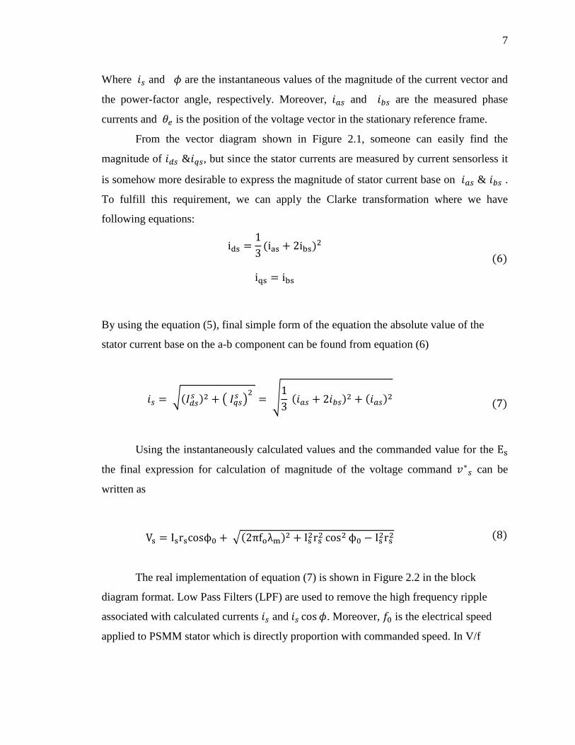
From the vector diagram shown in Figure 2.1, someone can easily find the
magnitude of 𝑚𝑑𝑠 &𝑚𝑞𝑠, but since the stator currents are measured by current sensorless it
is somehow more desirable to express the magnitude of stator current base on 𝑚𝑎𝑠 & 𝑚𝑏𝑠 .
To fulfill this requirement, we can apply the Clarke transformation where we have
following equations:
ids =13
(ias + 2ibs)2
iqs = ibs
(6)
By using the equation (5), final simple form of the equation the absolute value of the
stator current base on the a-b component can be found from equation (6)
𝑚𝑠 = �(𝐼𝑑𝑠𝑠 )2 + � 𝐼𝑞𝑠𝑠 �2
= �13
(𝑚𝑎𝑠 + 2𝑚𝑏𝑠)2 + (𝑚𝑎𝑠)2
(7)
Using the instantaneously calculated values and the commanded value for the Es
the final expression for calculation of magnitude of the voltage command 𝑣∗𝑠 can be
written as
Vs = Isrscosϕ0 + �(2πfoλm)2 + Is2rs2 cos2 ϕ0 − Is2rs2 (8)
The real implementation of equation (7) is shown in Figure 2.2 in the block
diagram format. Low Pass Filters (LPF) are used to remove the high frequency ripple
associated with calculated currents 𝑚𝑠 and 𝑚𝑠 cos𝜙. Moreover, 𝑓0 is the electrical speed
applied to PSMM stator which is directly proportion with commanded speed. In V/f

8
controlling method the ratio of the applied stator voltage and frequency is fixed and
constant.
Figure 2.2. Calculation of the voltage command
The preliminary drive configuration with the above-discussed voltage control
method is shown in Figure 2.3.
2.3. STABILITY ANALYSIS
One of the most important aspect of PMSM drive performance is its dynamic
response which means that whether it can exhibit a smooth and stable response to
different inputs at many various conditions which the PMSM may encounter in
practice.
Figure 2.3. Primary drive configuration with V/f control method
As an example, in this case, it must be verified in the case when the frequency of
applied voltage and current get changed, the output of system such as rotor speed should

9
gradually reach to the final value very smoothly although before reaching to this point it
may exhibit a negligible oscillatory behavior. In this part, stability analysis is going to be
performed for PMSM motor which does not have damper winding. To analyze the
stability of the PMSM under constant stator flux linkage control, the linearized PMSM
model is used. The eigenvalues of the state transition matrix of the linearized PMSM
model will reveal the stability behavior of the PMSM for all scenarios. Using the
linearized form of the equation accurate for PMSM, we will have the following
equations:
piqs =−iqsστs
− ωr
σ�λmLd
+ ids� + vs cos(δ)σLd
(9)
(
pids =−idsτs
− � σωr iqs� − vs sin(δ)
Ld (10)
(
pωr = 32J�n2�2�λmiqs + Ld(1 − σ)iqsids� − 1
J Bmωr −
n2J
Tl (11)
In (8) - (11):
τs = Ld/rs , σ =LqLd
(12)
The machine linear state equations (8)–(12) have the state form
𝑥̇ = 𝑓( 𝑥,𝑢) (13)
where is the vector of the machine state variables and is the nonlinear function of the
state and the inputs . The linearized system equations of this nonlinear system have the
form
𝛥𝑥̇ = 𝐴(𝑥)Δ𝑥 + 𝐵(𝑥)Δ𝑢 (14)

10
in which Δx is the perturbations matrix for state variables, A(x) is the state transition
matrix, Δu is the input perturbation matrix, and B(x) is the input matrix, finally, The
obtained linearized PMSM model can be written as in the matrix equation (13),
moreover, When deriving this model, it is considered that the input voltage and the
frequency to the PMSM are constant steady state values, i.e., perturbations Δvs=0 and
Δωe=0.
Using equation (13) which its derivation process is explained in [11] , some
inherent characteristic of the system such as stability issue can be studied from equation
(15).
The state transition matrix in (15) can be solved by using machine parameters and
the steady-state value of the machine variables (voltage, current, etc.) presented in table
2.1. In this thesis, machine parameters are chosen from [11], which are:
𝑝
⎣⎢⎢⎢⎢⎢⎡𝛥𝑚𝑞𝑠𝑟
𝛥𝑚𝑑𝑠𝑟
𝛥𝜔𝑟
𝛥𝛿 ⎦⎥⎥⎥⎥⎥⎤
=
⎣⎢⎢⎢⎢⎢⎢⎡ −
1𝜎𝜏𝑠
−𝜔0
𝜎−
1𝜎
(𝜆𝑚𝐿𝑑
+ 𝐼𝑑𝑠𝑟 ) −𝑉𝑠𝜎𝐿𝑑
sin (𝛿0)
𝜎𝜔0 −1𝜏𝑠
𝜎𝐼𝑞𝑠𝑟 −𝑉𝑠𝐿𝑑
cos (𝛿0)
32�𝑚2�
2
𝐽[ 𝜆𝑚 + 𝐿𝑑(1 − 𝜎)𝐼𝑑𝑠𝑟 ]
32 �𝑚2�
2
𝐽 𝐿𝑑(1− 𝜎)𝐼𝑞𝑠𝑟 −
𝐵𝑚𝐽
0
0 0 −1 0 ⎦⎥⎥⎥⎥⎥⎥⎤
�
𝛥𝑚𝑞𝑠𝑟
𝛥𝑚𝑑𝑠𝑟𝛥𝜔𝑟𝛥𝛿
�

11
Table 2.1. PMSM motor parameters which its loci plot is shown in Figure 1.6
𝑃𝑟𝑎𝑡𝑒𝑑 = 2.2 𝑘𝑘
𝑉𝑟𝑎𝑡𝑒𝑑 = 380 𝑉 𝜆𝑚 = . 48 𝑉. 𝑠. 𝑟𝑟𝑑−1
𝑇𝑙𝑟𝑎𝑡𝑒𝑑 = 12 N. m
𝑟𝑠 = 3.3𝛺 𝑃𝑃𝑃𝑃𝑠 = 6
𝐿𝑞 = 57.09 𝑚𝑚
𝐿𝑑 = 41.59 𝑚𝑚
𝐵𝑚 = 20.44 ∗ 10−4𝑁.𝑚. 𝑠. 𝑟𝑟𝑑−1
𝐽 = 10.07 ∗ 10−3𝑘𝑘.𝑚2
𝜔𝑟𝑎𝑡𝑒𝑑 = 1750𝑟𝑚𝑚𝑚
The paper also plots the calculated eigenvalues of the state transition matrix of
A(X) in (15), under no load, i.e., 𝑣𝑠 = 𝐸𝑚 (back electromotive force (EMF) produced by
rotor permanent magnets), as a function of the applied frequency. Figure 2.4 shows Loci
of the rotor poles under different load conditions. From below figure, the system goes
unstable when the electrical frequency greater than 15 Hz which means that if rotor
speed start increasing once time it pass this frequency the motor become unstable and its
speed get back to the zero)
Figure 2.4. Loci of the rotor poles under different load conditions, as a function of the
applied frequency

12
2.4. FREQUENCY MODULATION TECHNIQUE
The PMSM’s instability behavior after exceeding a certain applied frequency
observed in previous section is due to the nonexistence of rotor circuits (i.e., damper
windings) and, therefore, the weak coupling between electrical and mechanical modes of
the machine. The stator and rotor poles move away from each other and, after exceeding
a certain applied frequency, the poles of the system cross over to the instability region of
the s plane (right side of imaginary axis), having a small positive real part. Improvement
of instability issue can be achieved by a proper modulation of the applied frequency of
the machine.
The system becomes unstable during transient state where the motor tries to
follow an increase in speed. If the control system employed for PMSM drive just relies
on the open loop V/f method, the electrical speed and frequency are predefined and they
increase linearly without considering the transient and instantaneous condition PMSM
may face (there is not any simultaneous adjustment, and no flexibility), and in many
cases the real PMSM is not able to follow the predefined function which leads the system
toward instability condition. However, if the commanded electrical speed being able to
adjust itself base on its internal parameters perturbation, a stable behavior can be seen
from the system, the key parameter having dramatic changes during transient mode is
input power disturbance, and due to the fact that this parameter has direct relation with
rotor speed, stabilization loop can be implemented base on the idea of changing
commanded speed base on the input real power distribution. Therefore, 𝜔𝑒 is a new
variable added into the old A(x) matrix meaning that by choosing the appropriate
parameters a new transfer function can be derived. To find a new state space where
electrical speed is one its state, using input real power can be a good starting point. As a
matter of the fact, the applied frequency should be modulated as:
𝛥𝜔𝑒 = −𝑘𝑝𝛥𝑝𝑒 (16)
In the simulation,𝐾𝑝 = 2.4 is used. 𝛥𝑝𝑒 is the AC component of real input power which
must be filter out from DC value. Therefore, a HPF which has small cut off frequency
can be implemented to extract the AC component. 𝛥𝑝𝑒 can be written as

13
Δpe = ss+ 1
τh
Pe (17)
Pe = 32
Vs[iqsr cosδ − idsr sinδ] (18)
Where τhis the high-pass filter time constant, and in this simulation its value should be
τh= .064. Substituting Δpe from (17) in (16), and using equation (18) which present real
input power for a salient pole PMSM, the new state transition matrix can be calculated
which is fully described given in [11], and using the eigenvalues of new state space
matrix, it is easily possible to study the effectiveness of the stabilizing loop, which
modulates the applied frequency of the system. Figure 2.5 shows the rotor poles of the
system, which are obtained from the new A′(x), under different load conditions as a
function of the applied frequency.
Figure 2.5. Measured rotor speeds at different frequencies, under no load

14
Comparing Figures. 1.6 and 1.7 helps readers sense easily the effectiveness of the
stabilizing loop in the system, and it is obvious that adding stabilized loop which
modulate the input frequency of the input parameters of the motor can improve the motor
performance, and solve stability issue. Finally, Figure 2.6 show the block diagram of
stability loop.
The stability analysis described here is carried out for a salient PMSM which is a
general case. Therefore, performing the same procedures for round rotor PMSM, the
same results can be found.
2.5. EFFICIENCY OPTIMIZATION OF THE STABILIZED V/F CONTROL
In the previous section, it was shown that even with large load torque sudden
changes, the control was capable of maintaining stable operation in a wide frequency
range. However, further study indicated that the control is not optimized in terms of
overall system efficiency. The goal of this part is to improve the efficiency of the system
without sacrificing its stability features. Considering a round rotor PMSM, the torque
equation can be found from
𝑇𝑒 =3𝑃2
𝜆𝑚′ 𝑚𝑞 (19)
Figure 2.6. Derivation of the frequency modulation signal 𝛥𝑤𝑒

15
From the above equation, it can be seen that only q-axis current contribute in torque
production, and any d-axis current component only contributes to machine losses. As a
result, to improve the efficiency by keeping the d-axis current component close to zero,
nearly all of the currents absorbs by the PMSM have contribution in torque production.
The vector diagram of a PMSM in such an operating mode is shown in Figure 2.7. From
the vector diagram in Figure 2.7, it can be seen that if the d-axis current di is zero, the
current vector sI is aligned with 'mrλω . The reactive power also can be calculated from
equation (20).
Figure 2.7. Vector diagram of PMSM with maximum torque per amp
Qin =32
� Vqsiqs� = 32
� Vsiqs� (20)
(
Thus the current vector can be aligned with the back EMF vector by keeping the reactive
power drawn by the PMSM at zero. Since the reactive power in the electrical machines
are controlled by adjusting the magnitude of the stator voltage magnitude, a proportional-
integral (PI) controller can be used to generate the adjustment 𝛥𝑣𝑠∗ from input reactive
power which was found in equation (20).
16
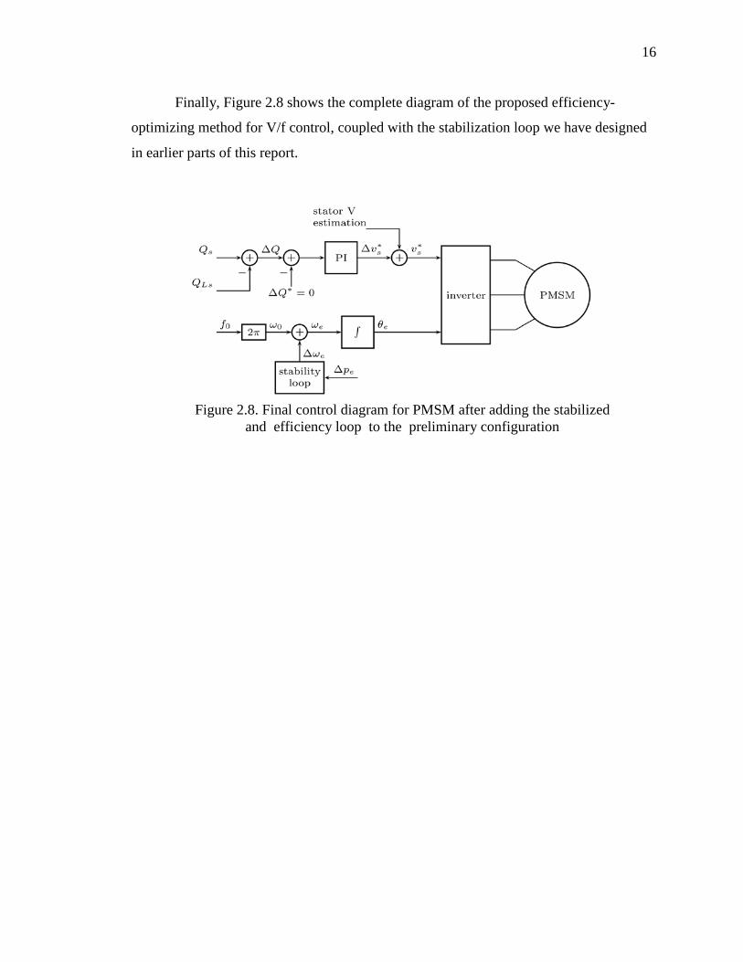
Finally, Figure 2.8 shows the complete diagram of the proposed efficiency-
optimizing method for V/f control, coupled with the stabilization loop we have designed
in earlier parts of this report.
Figure 2.8. Final control diagram for PMSM after adding the stabilized and efficiency loop to the preliminary configuration

17
3. DSP IMPLEMENTATION USING MATLAB/SIMULINK
3.1. INTRODUCTION
In the present day, time efficiency and flexibility are getting considered highly
important in research and product development throughout all industry fields. It also
applies to the development, implementation and testing of control algorithms for the
electrical motors. The rapid development in computer technology, computer science and
electronic during last decades allow electrical engineers and field researchers to easily
bring new, complex and efficient motors control algorithms into the practice which now
days mainly are implemented on microprocessors. As a result, it has led to a more energy
efficient use of electrical motors. Something that can help to the vast energy savings in
industrialized countries in which 30% to 40% of the electrical energy consumption is due
to the usage of electrical motors.
The process of programming a microprocessor and microcontroller for real time
applications is a tedious and time consuming task which must be done with aid of some
computer languages like C or Assembly. Furthermore, due to the lack of computer
programming skill, many power electrical engineers have difficulties with
implementation of a new efficient controlling method for a particular electrical machine.
However, during last decade a new approach for microcontroller programming has been
developed which is denoted Computer Automated Control System Design (CACSD) and
it mainly put emphasis on that embedded system programming should be performed in a
graphical environment and thus intuitive. As a matter of fact, in this new scheme, any
algorithms are implemented using graphical blocks containing invisible C or Assembly
codes and out of this, scheme code is auto generated by the CACSD program
environment. In general, this approach is a lot faster than writing the code by hand,
something allows developers to spend more time on improving the performance of their
programs instead of wasting the time to write and debug their C code errors.
The purpose of this chapter is to examine a rapid prototyping approach using a
CACSD to develop and implement a new motor control algorithm on a Digital Signal
Processor (DSP), but instead of programming the DSP in Assembly or C, the main
control algorithm will be performed in the Matlab/Simulink environment which is

18
developed by MathWorks𝑇𝑀. The control algorithm is implemented as block scheme in
Simulink, and out of this Simulink, Matlab can auto generate C-code needed to program
an embedded target like a DSP. Moreover, we also need to use Real-Time Workshop
(RTW) Embedded Coder to program our DSP.
It is worthy to mention here that the prime objective of this project is not to
develop a very efficient implementation in terms of motor step response and speed
reference tracking, but rather to develop a real time test platform that is easy to
understand and to evaluate the Mathworks CACSD environment from a user perspective.
The stabilized and efficient sensorless V/f method was implemented on a system
which Matlab & Simulink 2012b was installed on it. The additional packages required
for target specific code generation for the TI C2000 family are; Real Time Workshop
v8.0, Real Time Workshop Embedded Coder v5.0, Link to code composer v4.1 and
Target for TI C2000. In addition to the Matlab software, in order to program DSP, Code
Composer Studio v4 is needed to load generated C-code on the DSP.
An implementation of stabilized and efficient sensorless V/f in Matlab/Simulink
adapted for code generation with RTW can easily result in a model which is difficult to
follow its details. Therefore the model developed in the following sections is divided into
several subsystems, where each one is explained individually to make overall model
more intuitive and easy to follow.
3.2. TOP LEVEL
The overall DSP program for a stabilized and efficient sensorless V/f is shown in
Figure 3.1. The target preference block, here it is F28335 which is shown in grey color
block, specifies the setting of the processor. As a matter of the fact, this block tells EC
what sort of DSP is being programmed so that it initializes the right peripherals, uses the
correct operation frequency, knows how much memory is available, etc. It is important to
note that the placement of this block is important. When it is placed on the main screen,
everything in the simulation file will be built and compiled. However, if it be used inside
of a subsystem block, only that subsystem block will be built and compiled.
Figure 3.2 shows inside of eZdsp unit where user can chose his desired
microcontroller from wide range of different microcontrollers supporting rapid

19
prototyping of Matlab/ Simulink. It is also highly important to choose a proper CPU
clock which eventually has effect on the PWM switching frequency and ADC sampling
time. As a traditional method of C code programming of DSP in the code composer, we
normally import some predefined programs and some math libraries like
DSP2833x_PieCtril.c and DSP2833x_SysCtril.c and DSP2833x_Interrupt.c, mainly
written and developed by Texas Instrument and control default settings for different
peripheral units in a DSP, need to be load on DSP alongside of user main C program.
Finally, the Peripherals panel can be seen in Figure 3.2, is one of the most valuable
features of rapid prototyping which allow users to easily control such important variables
like defining eCAN bitrate and setting up I2C graphically through this panel. For more
information please refer to [12].
Figure 3.1. The top level in the implementation of DSP program in the Matlab/Simulink, left window, and the properties of the Hardware Interrupt block, right window

20
The block should also make a number of changes to the configuration parameters,
so the user should always double-check and make sure the parameters are correct. By
opening the configuration parameters, which is shown in Figure 3.3, from simulation tab
in Simulink, we can have access to broad hardware and software settings. But as simple
checking, user needs to ensure that the solver is set to Fixed-step and discrete, the fixed-
step size should remain auto. The hardware implementation page should show Texas
Instruments, C2000, and Little Endian. By expanding the code generation tree and
making sure that the system target file is “idelink_ert.tlc” on the code generation page.
Finally, the user needs to open the IDE Link page and select “Build” for the build action
option.
Figure 3.2. Target Preferences block can be fine in Simulink Library Embedded Coder>> Embed Targets

21
For the application where code efficiency has a high priority for the designer,
there are a couple of other things that can be done to improve the code output. For one we
can set objectives for the generated output code, such as execution efficiency, ROM
efficiency, and RAM efficiency.
In Figure 3.1, there are two function call subsystems in the scheme, the right side
one which is the main program is the part of the program in which the stabilized and
efficient sensorless V/f algorithm is implemented. The next block on the left side is ADC,
which is responsible to collect sample current data through the current sensors which are
located inside of the PMSM drive. ADC unit do scale and prepare current information for
the main program block. From Figure 2.1, someone can also easily find out that
subsystems are hooked up to the Hardware Interrupt block which it process interrupt
request issued by subsystems in the DSP program and will send trigger signals for
subsystem. In the Hardware interrupt block, see again Figure 3.1, the designer can set the
Interrupt Service Routine (ISR’s) that are to be used in the program and how these shall
be prioritized. The ISR generated by the Hardware Interrupt block are connected to the
Main program and ADC units which are triggered to be executed asynchronously once its
Figure 3.3. Configuration Parameters (simulation tab in Simulink)

22
interrupt is thrown. Since subsystems in our program are executed asynchronously all
blocks placed inside of them must have their sample time set to -1, which implies that the
sample time is inherited.
The right part of Figure 3.1 shows the properties pane of the Hardware Interrupt
Block. To generate an ISR the designer should choose the four parameters, specified on
row one to four, that are used by Matlab to describe an interrupt. The first two parameters
are the CPU and PIE interrupt numbers, found on row one and two separately. These
numbers correspond to a position in the F28335 interrupt table which is shown in Figure
3.4.
In right window of Figure 3.1, two ISR are initialized, here presented in
coordinated form (CPU number, PIE number). The first interrupt has coordinates (1, 1),
which corresponds to an event coming from the ADC module. Interrupt number two has
coordinates (3, 1) which correspond to an event coming from the first ePWM module and
it triggers the execution of the Main Program subsystem. Moreover, on the third row the
Simulink task priority is set, a low value correspond to a high priority. Here the Main
Program subsystem has a higher priority since it is the main task and thus forms the base
rate of the model. Figure 3.4 shows F2833x PIE interrupt assignment table which specify
related peripheral units interrupt numbers, for more information about interrupt unit
inside of the C2000 F2833x please see [13]. The reader should also be aware that
process of setting the interrupt units is not yet over because what have been discussed up
to this point are related to top level part of a DSP program. To set up the interrupt
request, we shall go into subsystem under layer where major DSP peripheral units like
ADC, ePWM and CAN are located.
Finally, on the top level page, it can be seen that there are rate transition blocks
connected between output and input of ADC and Main Program subsystems. This is a
requirement for all signal paths between blocks running on different sample rates. The
rate transition block improves the data integrity in the system.

23
Figure 3.4. Interrupt vector table
3.3. ADC UNIT AND SUBSYSTEM
Figure 3.5 depict inside of ADC subsystem. As it was mentioned in the previous
part, C280/C2833x ADC peripheral block inside of ADC unit first start reading the
current signals, and then scale them up to their actual current magnitude and as last and
most important step filter out undesirable noises associate with current signals. To do
noise cancelation, a LPF with 5 Hz cut off frequency is employed. However, even using
this low pas filter; we still observe a major noise component on current signal. Therefore,
to better address and alleviate undesirable noise effect, a series of unit delay blocks are
employed at the output side of LPF. Figure 3.6 clearly shows how these block is
implemented using some delay units. As a matter of the fact, using delay units, which
their delay time is defined by trigger unit. Having access to about 25 sample points make
it possible to find the sum and then calculate the average value. Therefore, after using
these noise cancelation strategies what we expect to see at the output of the ADC
subsystem is pure sinusoidal waveforms with very small proportion of noise.
On Figure 3.7, properties panel of the ADC module is shown. C280/C2833x ADC
consist from two independent ADC channels A/B which have their own control time base
and they are capable to operate in Simultaneous mode and sequence mode. By selecting

24
Simultaneous Sampling for the sampling mode we can convert 2 independent analogue
input signals simultaneously.
If Sequential Sampling is chosen only one multiplexed input channel (for example
A) is converted at the time. By selecting Single Sequence Mjode (or “Start/Halt - Mode”)
the Auto sequencer starts at the first input trigger signal, performs the predefined number
of conversions and stops at the end of this conversion sequence then to wait for a second
trigger. In continuous mode the Auto sequencer starts all over again at the end of the first
conversion sequence without waiting for another trigger input signal.. The conversation
mode is sequential and will post interrupt at the end of conversation meaning that it will
stop converting analog data to digital until it receives a new trigger signal. Furthermore,
ePWMxA (orange block in Figure 2.5.) should issue an interrupt request for the ADC
unit to get a trigger signal from top layer of DSP program. Further discussion will come
up in the next section where the main program will be explained in great details. For
obtaining more information about C2000 F2833x ADC please see [14].
Figure 3.5. ADC subsystem implementing measurement and scaling

25
Figure 3.6. Unit delay implementation using 6 unit delay blocks
3.4. MAIN PROGRAM SUBSYSTEM
Figure 3.8 represents the main stabilized and efficient V/f algorithm implemented
for a PMSM machine drive. For the sake of easiness in understanding the main
functionality of the program, we explain the program in detail step by step.
Figure 3.7. Show the properties of the ADC module

26
Figure 3.8. Implementation of sensor less stabilized efficient V/f for PMSM drive in Main Program subsystem
Since a sensorless method is being used, we should estimate the electrical rotor
position from the commanded speed, but it is highly important for the reader to know that
this angle is not necessarily same as the real rotor position. Therefore, it could be possible
that the electrical angle is different than real rotor position, but in steady state value
should be the same. In Figure 2.8, the parameter fb defines the maximum rotor speed as a
step function, it is connected to an adjustable rate limiter controlling the desirable rise
time of PMSM rotor. In here, the purpose of rise time is the amount of time rotor should
spend to accelerate from zero speed to get maximum speed which is defined by fb. After

27
importing the electrical speed into the program, in the following the calculation of
electrical angle is implemented which is shown in Figure 3.9.
Figure 3.9. Calculating the electrical angle from the motor speed and program sampling
time
The following equation is used in electrical angle calculation:
θe,t = θe,t −1 + ωeTsec (21)
The unit delay will keep the previous sample point and send it for comparison unit. Using
a switch block we can reset electrical angle whenever its value reaches 2π . The output
will be electrical angle which will be used in other subsystems inside of the main
program.
As it was discussed in the first section, voltage magnitude must be calculated
from speed command and current magnitude which can be derived from following
equation
Vs = Isrscosϕ0 + �(2πfoλm)2 + Is2rs2 cos2 ϕ0 − Is2rs2 (22)
Equation (21) is implemented inside of the voltage magnitude subsystem which is shown
in Figure 3.10. It is noteworthy to mention here that all blocks have inherited (-1)
1Qe
z
1
>= single
0
2*piT_sec
1we

28
sampling time. The IF function block assure that all the time the term under square is
positive. The assigned value for 𝜆𝑚 and 𝑟𝑠 is presented in section 2 where all PMSM
motor parameters is presented detail.
Figure 3.10. Finding voltage magnitude from frequency and a-b phases current
In equation (21), 𝐼𝑠 𝑐𝑃𝑠 𝜙0 𝑟𝑚𝑑 𝐼𝑠 𝑠𝑚𝑚 𝜙0 are q and d stator current components
which are calculated using abc/dq transformation block which is depicted in downside of
the Figure 3.5. Finally, this block will give 𝐼𝑞and 𝐼𝑑 which are critical parameters for V/f
algorithm. As a matter of the fact the real and reactive power will be calculate using them
and in the later part in which we implement efficiency loop, we will see that by
regulating𝐼𝑑 we can make it goes to zero. Figure 3.11 is showing abc/dq transformation
and relevant equations.
Stabilization loop is also implemented based on the expected functionally which
was described earlier in the first chapter. It must filter out undesirable DC component of
the input real power in order to be capable of generating 𝛥𝜔𝑒, which is required for
stabilization of PMSM, based on perturbation in the input real power. Figure 3.12 shows
how 𝛥𝜔𝑒 is generated from AC portion of input real power and commanded speed.

29
Figure 3.11. Park transformation
Figure 3.12. Stabilization loop implementation
Efficiency loop also is developed from the idea that by controlling the reactive
power, 𝐼𝑑 current can be controlled and set to the zero. A PI controller can fulfill the need
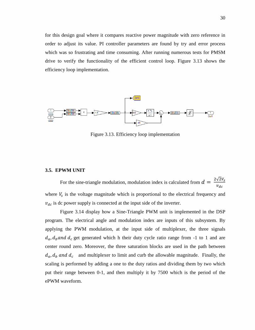
30
for this design goal where it compares reactive power magnitude with zero reference in
order to adjust its value. PI controller parameters are found by try and error process
which was so frustrating and time consuming. After running numerous tests for PMSM
drive to verify the functionality of the efficient control loop. Figure 3.13 shows the
efficiency loop implementation.
Figure 3.13. Efficiency loop implementation
3.5. EPWM UNIT
For the sine-triangle modulation, modulation index is calculated from 𝑑 = 2√2𝑉𝑠𝑣𝑑𝑐
where 𝑉𝑠 is the voltage magnitude which is proportional to the electrical frequency and
𝑣𝑑𝑐 is dc power supply is connected at the input side of the inverter.
Figure 3.14 display how a Sine-Triangle PWM unit is implemented in the DSP
program. The electrical angle and modulation index are inputs of this subsystem. By
applying the PWM modulation, at the input side of multiplexer, the three signals
𝑑𝑎,𝑑𝑏𝑟𝑚𝑑 𝑑𝑐 get generated which h their duty cycle ratio range from -1 to 1 and are
center round zero. Moreover, the three saturation blocks are used in the path between
𝑑𝑎,𝑑𝑏 𝑟𝑚𝑑 𝑑𝑐 and multiplexer to limit and curb the allowable magnitude. Finally, the
scaling is performed by adding a one to the duty ratios and dividing them by two which
put their range between 0-1, and then multiply it by 7500 which is the period of the
ePWM waveform.

31
Figure 3.14. Display of ePWM unit inside of the main program
In machine drive application, it is common to choose switching frequency
somewhere between 5 kHz-10 kHz, for this application chosen switching frequency is
10 kHz. It was mentioned earlier that the CPU clock is set for 150MHz inside of the
F28335 eZdsp block, therefore in order to generate signal of 10 kHz at line ePWM1-6A,
the TPRD which define signal frequency should be calculated from following equation:
TBPRD =12
×fSYSCLKOUT
fPWM × CLKDIV × HSPCLKDIV=
150M2 ∗ 10K
= 7500 (23)
In the last equation, due to the fact that ePWM counting mode is set in Up-Down mode, a
2 factor is used in the denominator. The properties of the PWM block are shown in
Figure 3.15. Here it is possible to set practically all features belonging to the PWM
module of the F2833xin a simple graphical way. The controllable features ranges from
setting of timer period, duty cycle, dead band generation, symmetrical/ unsymmetrical
waveforms, to the control of then in the PWM cycle ADC conversations are to occur.
In Figure 3.15, left window shows a pane in which the basic ePWM settings
needed to activate an ePWM unit are located. Register TBPRD defines the length of a
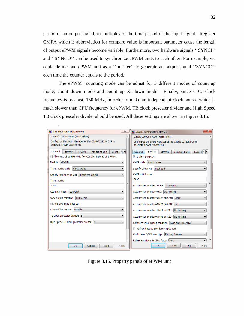
32
period of an output signal, in multiples of the time period of the input signal. Register
CMPA which is abbreviation for compare value is important parameter cause the length
of output ePWM signals become variable. Furthermore, two hardware signals ‘’SYNCI’’
and ‘’SYNCO’’ can be used to synchronize ePWM units to each other. For example, we
could define one ePWM unit as a ‘’ master’’ to generate an output signal ‘’SYNCO’’
each time the counter equals to the period.
The ePWM counting mode can be adjust for 3 different modes of count up
mode, count down mode and count up & down mode. Finally, since CPU clock
frequency is too fast, 150 MHz, in order to make an independent clock source which is
much slower than CPU frequency for ePWM, TB clock prescaler divider and High Speed
TB clock prescaler divider should be used. All these settings are shown in Figure 3.15.
.
Figure 3.15. Property panels of ePWM unit

33
Furthermore, Right window in Figure 3.15 also show the action qualifier unit. Whenever
the ePWM counter value reach to the compare value which is specified by CMPA
register, the unit can change the value of the output signals Figure 3.16, the event trigger
pane determine the source of the interrupt and manage interrupt request
In switched mode power electronics, a typical configuration to drive a 3-phase
system is shown in the Figure 3.17. A typical system consists of a 3-phase current or
voltage injection circuit, in which a pair of power switches per phase is controlled by a
sequence of PWM - pulses. A phase current flows either from a DC bus voltage through a
top switch into the winding of a motor or via a bottom switch from the motor winding
back to ground. Of course, we have to prevent both switches from conducting at the same
Figure 3.16. Property panels of ePWM unit

34
time. A minor problem arises from the fact that power switches usually turn on faster
than they turn off. If we would apply an identical but complementary pulse pattern to the
top and bottom switch of a phase, we would end up in a short period in time with a shoot-
through situation.
Figure 3.17. A typical configuration to drive a 3-phase system consist of a DC bus and
3- phase full bridge
Dead-band control provides a convenient means of combating current “shoot-
through” problems in a power converter. “Shoot-through” occurs when both the upper
and lower transistors in the same phase of a power converter are on simultaneously. This
condition shorts the power supply and results in a large current draw. Shoot-through
problems occur because transistors turn on faster than they turn off and also because
high-side and low-side power converter transistors are typically switched in a
complimentary fashion. Although the duration of the shoot-through current path is finite
during PWM cycling, (i.e. the transistor will eventually turn off), even brief periods of a
short circuit condition can produce excessive heating and stress the power converter and
power supply. To address this issue, the best approach to shoot-through control separates
transitions on complimentary PWM signals with a fixed period of time. This is called
C A B

35
dead-band. While it is possible to perform software implementation of dead-band, the
F2833x offers on-chip hardware for this purpose that requires no additional CPU
overhead. Compared to the passive approach, dead-band offers more precise control of
gate timing requirements.
In Figure 3.18, complementary pulse sequences having different patterns can be
selected from dead band polarity and dead band value will be defined using RED and
FED registers. Figure 3.18 also contains all definable pattern can be used for different
application. Finally, for getting more information about ePWM unit please see [15].
3.6. ECAN UNIT
Finally, in order to see whether the proposed stabilized and efficient V/f control
algorithm for PMSM is functional, some critical parameters like input real power,
reactive power and q component of stator current need to be calculated and be compared
for different cases where the stabilized and the efficiency loop may or may not be used.
Figure 3.18. Dead-band waveforms for typical cases

36
Due to the fact that some of these parameters are math defined elements and also
some other like input real power or reactive power cannot be measured by oscilloscope,
user must be capable to communicate directly with DSP using one way from different
defined communication protocol for DSP. The F28335 DSP supports three different
communication protocols that can be used in communication between the DSP and
Matlab. These are CAN, SCI and RTDX (Real Time Data Exchange). For these thesis,
the CAN communication is selected due to its advantages it has over others
communication methods. This portion of the thesis is dedicated to explain ECAN
peripheral unit which was used in the DSP program.
3.6.1. Basics. Controller Area Network (CAN) is a serial network technology that
was originally designed for automotive industry, especially for European cars, but has
also become a popular communication protocol in industrial automation as well as other
applications. The CAN bus is primarily used in embedded systems, and as its name
implies, is a network technology that provides fast communication among
microcontrollers up to real-time requirements which eliminate the need for the much
more expensive and complex technology of a Dual-Ported RAM. It also grants high
speed real-time communication and noise immunity in the noisy environment commonly
found in a vehicle. [16] CAN is a two-wire, half duplex, high-speed network system, that
is far superior to conventional serial technologies such as RS232 in regards to
functionality and reliability and yet CAN implementations are more cost effective.
In general Controller Area Network has the following features:
• Is a high-integrity serial data communications bus for real-time applications
• Is more cost effective than any other serial bus system including RS232 and
TCP/IP
• Provides better ease of use than any other serial bus system
• Operates at data rates of up to 1 Megabit per second
• Has excellent error detection and fault confinement capabilities
• Has the ability to function in difficult electrical environments
• Is now being used in many other industrial automation

37
A typical physical CAN bus consist of two wires terminated at both ends by 120
Ω resistors in addition to a reference wire. The system uses this three wire setup for
differential signals for better noise immunity. The old and obsolete system used flat
ribbon cables for communication; each cable was directly connected to its destination.
The use of multi-wire systems leads to higher weight, higher cost, higher complexity and
lower reliability due to the number of wires. Figure 3.19 displays a comparison between
CAN bus set up and older multi-wire setup.
Figure 3.19. Comparison between older multi-wire setup and typical Can bus set up

38
So with this network system, each sensor or controller is now a node on the bus
and can communicate to any other node on the network. Figure 3.20 shows a typical node
setup, where the system have a CAN controller and CAN transceiver in each node. The
CAN controller is where the message database is kept, which decodes and encodes all of
the data being sent and received from that node to the network. The CAN transceiver
actually transmits and receives the messages on the bus.
Figure 3.20. CAN node example
3.6.2. Message Frame Architecture. Various types of messages, or frames, exist
in the CAN protocol. These types include: data, remote, error, overload, and inter space
frames. Only the data and remote frames are set by the user, everything else is set by the
hardware and come into the action whenever there is a fault or error on the CAN bus in
order to protect form data accuracy and integrity. In Figure 2.21, standard data frame is
shown, or message. Each message has a unique ID, a data field, and other header
information.

39
SOF (1 Bit)
The dominant Start of Frame (SOF) bit represents the start of a Data/Remote
Frame. A CAN node, before attempting to access the bus, must wait until the bus is idle.
An idle bus is detected by a sequence of 11 recessive bits ( 11 zero bits) which is the
sequence of ACK Delimiter bit in the Acknowledgement Field (1 bit), the End of Frame
Field (7 bits) and the Intermission Field (3 bits).(Figure 3.21)
Arbitration field ( 12 or 32 bit)
The arbitration field contains of two components:
• 11/29 Bit Message Identifier, first Bit is MSB, and the CAN message ID can be
11 or 29 bits long. RTR (Remote Transmission Request) indicates either the
transmission of a Data Frame (RTR = 0) or a Remote-Request Frame (RTR = 1).
A low message ID number represents a high message priority. For example, a
message that its ID number is 0x000 must be the most important message in CAN
database library which have the highest priority to access the CAN bus for data
submission. The total length of the arbitration field is 12 bits when an 11 bit message
identifier is used. As shown in picture 3, the total length of the arbitration field will be 32
bit with a 29 bit identifier
Figure 3.21. CAN data frame for 29-Bit extended format

40
Control Field ( 6 Bits)
The 4 LSB bits of the Control Field specify the length of the data block (DLC =
Data Length Code), the MSB bit (IDE = Identifier Extension) indicates either standard
11-Bit format (Bit = 0) or 29-Bit extended format (Bit = 1). The Data Length Code
(DLC) is normally set to a value between 0 and 8 indicating a data field length between 0
and 8 bytes.
Data Field ( 8 Bits)
Data field is most important part of data frame message carrying information from
different nodes of different subsystems. The data must be imported in hex format. As we
will show in the later part, in real application, it is common t message o packed signals
into a single message in order to minimize the message numbers defined for CAN
database; therefore, the start bit of each signal is critical for a receiver node to easily
distinguish and unpacked its relevant signals out of a specific message.
3.6.3. Message Broadcasting and Error Detection. The broadcasting of
messages in a CAN network is based on a producer-consumer principle. One node, when
sending a message, will be the producer while all other nodes are the consumers. All
nodes in a CAN network receive the same message at the same time. Each node “listens”
to the network bus and will receive every transmitted message on the CAN bus. The
CAN protocol supports message filtering meaning that the receiving nodes will only react
to data that is relevant to them and are defined in their database library otherwise nodes
ignore the irrelevant messages. CAN assume that all messages are compliant with the
defined standard and if they do not, there will be a corresponding response by all nodes in
the network for Error Detection. If the consistency is not acknowledged by any or all
nodes in the network, the transmitter of the frame will post an error message to the bus
and will not grant permission to nodes for their message transmission. Moreover, If
either one or more nodes are unable to decode a message, either detect an error in the
message or are unable to read the message due to an internal malfunction, the entire bus
will be notified of the error condition.

41
3.6.4. Canoe Software. Each node attached to the CAN bus needs a Host
Processor, CAN Controller, and Transceiver in order to receive and send CAN messages.
The Host Processor decodes the messages using a database which is defined by user to
extract real data from received binary digits. For this project The Vector CANoe software
along with a Vector CANcaseXL hardware interface was used to monitor and analyze the
on-line operation of the CAN network. CANoe is a development and testing software
tool from Vector Informatik GmbH. The software is primarily used by automotive
manufacturers and electronic control unit (ECU) suppliers for development, analysis,
simulation, testing, diagnostics and start-up of ECU networks and individual ECUs.
Figure 3.22 shows inside of the CANOE software where the user can import any CAN
database into the software which means that any message exist on the Can bus and is not
defined for the CAN database cannot be motorized and be measured by the user.
Moreover, I- Generator is a block in which user can manually define a CAN message out
of the CAN data base library. As an example, the reader can imagine that in the DSP
program where the user should define a commanded speed for PMSM, instead of using a
constant Simulink block, it is possible to import CAN message from CANoe into the
DSP program. Moreover, the user doesn’t supposed to build a new DSP program for each
new commanded speed, which is time consuming process, and he can simultaneously
change the speed command while the DSP program is running to verify the V/f
algorithm functionality for different speeds. The CAN database for the system was
developed using the Vector CANdb++ software. The CANdb++ is a data management
program which can be used to create and modify CAN databases. The CAN Controller
stores received data bits serially until an entire message is available and then transfers it
to the Host Processor. The Transceiver acts as a voltage level shifter and adapts signal
levels from the bus voltage level to the voltage level that the CAN controller expects.
For further information about making up a CAN database using CANdb++ and setting
up the CANoe software for monitoring the CAN messages, please refer to the following
references [17, 18].

42
Figure 3.22. CANoe configuration window
3.6.5. Can Using Simulink’s Embedded Coder. This section will provide a
basic guide to get the F28335 DSP programmed to use CAN using Simulink’s
embedded coder. As a first step the user is supposed to set a baud rate which he has
already defined for CANoe software. By opening up the target preferences block in
Simulink and navigating to the eCAN_A section under the Peripherals tab the baud rate
can be define for the CAN bus, as shown in Figure 3.23. To get idea about how to set a
particular bite rate please see the reference [12].

43
Figure 3.23. CAN A preferences
Next users need to setup the Vector CANcaseXL box ,Figure. 3.24, to operate at a
1 Mbps baud rate as well. To do this, please hook up the box to the PC and open the
Vector Hardware application. Backing to the Figure 3.22, by double clicking on the
Network can bus; the baud rate can be also defined for the software. Finally a CAN
harness 2 wire cable attached to the 9 pin D-sub pin out which is shown in figure 3.25
should be connected between DSP and CAN vector box.

44
Figure 3.24. Vector CAN box
Fig. 20: D-sub pinout
CAN communication with Embedded Coder is done using four blocks: CAN Figure 3.25. D-sub pin out

45
CAN communication with Embedded Coder is done using four blocks: CAN
Pack, CAN Unpack, eCAN Transmit, and eCAN Receive. The first two blocks are found
in the Target Communication submenu of the C2000 branch in Simulink’s library
browser. The latter two blocks are found in the C28x3x submenu. The CAN Pack block
(Figure 3.26) takes Simulink values and packs them into a message that is transferred
over the network using the eCAN Transmit block. If the user be lucky enough to be using
a 32-bit version of Matlab/Simulink there is an option to load the .dbc file you created
earlier to fill in all these options; otherwise you have to fill them in by hand.
Figure 3.26. CAN Pack Block

46
By selecting “manually specified signals” from the “data is input as” drop-down menu
then all the information you enter has to match what was entered into your database file.
The eCAN Transmit block settings are also pretty straight forward. The dialog
menu shown in Figure 3.27 should have similar setup options to what you will be using.
Mailbox number is a given number from 1-12, and it can be random number. The user
can choose between the A and B CAN bus. The message identifier should be the same
message ID in hex, minus the “0x” from the database file which was defined by
CANdb++ and was imported into the CANoe software. The box ‘’ post interrupt when
message is transmitted’’ should also be checked [15] help to set up a eCAN unit for DSP.
Figure 3.27. eCAN Transmit block

47
4. SIMULATION AND EXPERIMENTAL RESULTS
4.1. SIMULATION
In order To verify the accuracy and performance of the both stabilized loop and
proposed efficiency-optimizing control technique, simulation tests have been conducted
using the Simulink of the MATLAB. The PMSM parameters used in the simulation is
presented in the table 2.2.
Table 2. 2. PMSM motor parameters which were used in experimental tests
𝐿𝑑 = 𝐿𝑞 = 1.9𝑚𝑚 𝑅𝑟𝑡𝑃𝑑 𝑃𝑃𝑤𝑃𝑟 = 15 𝐾𝑤 𝑟𝑟𝑡𝑃𝑑
𝜆𝑚 = . 278 𝑆𝑝𝑃𝑃𝑑 = 1750 𝑟/𝑚𝑚𝑚
𝐽 = 15 ∗ 10−3𝑘𝑘.𝑚2 number of poles= 6
𝐵𝑚 = 20.4 ∗ 10−3𝑁.𝑚. 𝑠 𝑟𝑠= . 149
𝐼𝑟𝑎𝑡𝑒𝑑= 50 A
As it was discussed in the first chapter, PMSM motors that are not equipped with
damper winding have serious stability problems during transient conditions like for
example, during time motor start up , the rotor may capable to drive out from zero
speed, but before reaching to the commanded speed it will lose synchronization. Another
common instability scenario is when the amount of load torque exerted on PMSM rotor
shaft suddenly and abruptly get changed, commonly happen in field of motor application
leading motor into the instability situation. Therefore, the first test is to examine the
effect of stability loop on the PMSM start up using stabilized loop. Figure 4.1 shows the
measured rotor speed of the machine, when the machine is ramped up to different
frequencies under no load, for the sensorless V/f controller where the stabilization loop is
not utilized From Figure 1.3, the stable operation of the machine at low frequencies and
the unstable operation at high frequencies is evident, as expected from the stability
analysis and the loci diagram was shown in Figure 2.5.

48
The same test was carried out with the drive configuration shown in Figure 2.6,
with the stabilizing loop in the system. The stabilizing loop parameters which were used
to calculate the eigenvalue plots in Figure 2.5 were used in the drive system. Since the
stable operation of the machine was possible at low frequencies the stabilizing loop was
added to the system. Figure 4.2 shows the results. Comparing this figure with Figure 4.1,
the effect of stabilized loop should be tangible for the readers indicating stabilization loop
is correspond to the damper winding on rotor cage of synchronized electrical machines.
Figure 4.1. Measured rotor speeds at different frequencies, under no load, without stabilizing loop in the system
f = 10 Hz
f = 43.75 Hz
f = 87.5 Hz

49
In the next simulation test, the effect of adding efficiency loop to a stabilized V/f
sensorless control method for PMSM is studied by measuring various motor parameters
for two different scenarios. In the first case, a stabilized V/f is not utilized with efficiency
loop while in the second test efficiency loop is employed in control loop.
In the first scenario, the machine is started at zero speed and load torque, it then
ramps up the speed towards half of the rated value, which corresponds to an electrical
frequency of 98.43 Hz which is equivalent to 940 rpm. At t = 3 seconds, the load torque
is stepped to the rated value of 15 N.m. Later on, at t=5 the load torque magnitude
increase to 25 N. Finally, at t = 7 seconds, the load torque is stepped back to zero. The
simulation results are presented in Figures 4.3 - 4.9 and in all these figure the green line
diagram represent the results of test in which efficiency loop is employed.
f = 87.5 Hz
f = 43.75
f = 10 Hz
Figure 4.2. Measured rotor speeds at different frequencies, under no load, with stabilizing loop in the system

50
Figure 4.3, support our earlier claim that by controlling the reactive power and
keeping its value to the zero, we should able to see changers in magnitude of input real
power. It is noteworthy to mention that as the amount of load torque applying on motor
shaft increase, the magnitude of input real power increase consequently and the benefit of
using efficiency loop become more apparent due to the fact that power losses get much
smaller compare to the low and light load torque. By making comparison between 2
diagrams in Figure 4.3, it is clear that by using the second method, it is possible to save
up the input power up to the 10%, and reduce the machine losses. Because the q-axis
current is directly proportional to the electrical torque, zero d-axis current means that the
stator current magnitude is at its minimum. Moreover, Base on the result presented in
Figure 4.5, in order to control the reactive power, the voltage magnitude need to be
regulated. In fact, in any type of synchronized machine starter voltage magnitude is
proportional with reactive power.
Base on simulation results of Figure 4.7 and 4.8, at 25 N.m torque, the q-axis
current has a significant magnitude. However, the d-axis current is also very large, even
though it does not have any contribution to torque generation, and it cause inclination in
power loss, but in the next test, the efficiency optimization algorithm is added to the
simulation and the same test procedure is followed as in the first test. Comparing results
in Figure 4.7 has almost identical waveforms for rotor speed, torque, and q-axis stator
current. One of the differences lies in the waveforms of the d-axis current, which is
maintained at near zero in Figure 4.8.
Finally, as can be seen from Figure 4.9, after the speed ramp, the motor is able to
maintain a constant speed even with large step changes in load torque. The operation is
stable in the whole speed and torque range regardless of efficiency loop usage in the
control loop. In all following graphs, the green color one shows the stabilized V/f which
efficiency loop controller is employed while the blue one represent the stabilized V/f
without efficiency loop controller.

51
Time [s]
Time [s]
Figure 4.4. Comparison of input reactive power
Figure 4.3. Comparison of input real power

52
Time [s]
Time [s]
Figure 4.6. Comparison of stator current magnitude
Figure 4.5. Comparison of stator voltage magnitude

53
Time [s]
Time [s]
Figure 4.7. Comparison of stator current q component
Figure 4.8. Comparison of stator current d component

54
4.2. EXPERIMENTAL RESULTS
Figure 4.10 and 4.11 show the lab experimental set up for this thesis. The Matlab
2012 has been installed on the lab computers with all the toolboxes and subsystems
which are required for C2000 DSP rapid prototyping. Moreover, the dc motor is driven
by a DCS800 ABB drive while the PMSG drive is a custom made drive built by the team
using a TMS320F28335 DSP from Texas Instrument and a Semikron SKS 83F B6CI 44
V 12 inverter.
To be able to run PMSM and control it based on the program running on its DSP,
a 320 V dc supply must feed the PSMSM drive which is provided by constant dc power
supply shown in Figure 4.10. Both PMSM drive and DC drive support the CAN
communication, and the PMMS calculated and measured motor parameters are read out
of the CAN port was integrated into the PMSM drive. Furthermore, it was very crucial
for the experimental tests that being able to apply load torque on PMSM shaft abruptly to
examine the dynamic behavior of PMSM machine under heavy load torque changes
while a sensorless V/f is supposed to control its speed. For this purpose, Advanced
Time [s]
Figure 4.9. Comparison of rotor mechanical speed

55
DCS800 ABB drive allow the user to communicate with dc machines by reading dc
machines measured signals like mechanical speed or by sending the user command such
as load torque ,which is our primary concern in this case, through the CAN protocol
communication.
Finally, the experimental results are presented in Figures 4.11 – 4.18, all the
signals are measured and recorded in CANOE software originally, but to improve result
quality and make it more appealing for the readers the recorded data was transformed into
the Matlab and was plotted regain. In all following graphs, the green color one shows the
stabilized V/f which efficiency loop controller is employed while the blue one represent
the stabilized V/f without efficiency loop controller.
Figure 4.10. Lab set up for efficient and stabilized V/f for PMSM machine

56
Time [s]
Time [s] Figure 4.12. Comparison of input reactive power
Figure 4.11. Comparison of input real power

57
Time [s]
Time [s]
Figure 4.14. Comparison of stator voltage magnitude
Figure 4.13. Comparison of stator current magnitude

58
Time [s]
Time [s]
Figure 4.16. Comparison of stator current d component
Figure 4.15. Comparison of stator current q component

59
Time [s]
Time [s]
Figure 4.18. Comparison of applied load torque
Figure 4.17. Comparison of rotor mechanical speed

60
4.3. ISSUES ENCOUNTERED DURING THE IMPLEMENTATION
When working with a relatively new technology such as automated generation for
embedded targets some problematic issues are to be expected. Here, it is important to
distinguish issues and the problems they cause from one another.
The most important issue is the reliability of the generated cod, i.e. that the code
actually has the anticipated functionality. This has never been a problem through this
project; the generated code has always functioned correctly and there have never been
any compilation errors. This is most likely due to the Target Language Complier (TLC)
in RTW which generates the code for all the different processor family packages, of
which Target for TI C2000 is one. Hence a lot of development effort has been spent on
the TLC and it appears to be very mature technology.
4.3.1. Software Issue. What has been an issue in the project are which blocks
that are supported by code generation and which are not. The main problem is that all
Simulink blocks that support code generation are not gathered in one or several block
sets. Of course all the blocks that supports code generation, but to design the model more
blocks are need such as summing and delay blocks, these blocks are found in the standard
Simulink libraries. One illustrative example is that the unit delay block is supported but
the integer delay block is not, even though they are basically identical in functionality.
In the case that user wants to use a fixed point DSP, another problem can happen
through project development. The problem is that some of the standard Simulink blocks
that support code generation does not support fixed point numbers. When using these
clocks the signal must first be converted to integer or floating point then passed on to the
block and then after the block be converted back to fixed point, something that of course
highly degrades the efficiency of the generated code for the fixed point digital signal
processor families. However the major issues encountered has not been regarding
whether or not blocks support code generation or not but rather which DSP settings that
are supported in the code generation. A tangible example of this problem is how the two
hardware interrupt were initialized in the model that was developed. The interrupt
generated in the ADC module, see section, and was initialized by selecting the post
interrupt at end of conversion option in the properties pane of the ADC block.

61
The interrupt generated by the ePWM module was initialized in completely
different and not very intuitive way, as described in section 2.2. This inconsistency in
which settings that are implemented in different modules is quite confusing and
disturbing for the designer.
When working in a rapid prototyping approach it is desirable for the designer to
have the possibility to alter parameter values in real time or at least to alter them without
rebuilding the entire program. This feature is possible in Matlab when using Simulink
external mode, see [19], which enable logging and parameter tuning. However, this
feature is only available using the CAN communication protocol which is getting used
for implementation in this project. Particular for this project, using the CAN
communication, the user easily can change the commanded speed of PMSM at any time
after code generation whiles the test running.
It is noteworthy to mention here that parameter tuning and external mode is not
compatible with IQmath/DMC blocks even when using CAN communication. This
means that when the gains in for example a PID controller is to be changed, the whole
program has to be regenerated.
4.3.2. Debugging. The debugging process when working with automated code
generation is as anticipated fairly different compared to code written in the usual way. In
the standard design process most syntax errors are found during the compilation of the
program and are corrected in an iterative process unit the code compiles with the design
rules.
In Matlab the syntax errors are found before the code is compiled, as Matlab
executes the build command it checks the Simulink model and controls whether design
rules are obeyed before he code is generated. Instead of an error message from the
compiler the designer gets an error message from Simulink and the build process is halted
before the code generation starts. Therefore there are seldom compilation errors.
The second part of the debugging process concerns the code functionality. Here
the automated code generation has both advantages and disadvantages. The main
advantage is the fact the code is auto generated. Thus registers, counters and memory
sections are initialized correctly and without human mistakes. Since these are the main
sources of functionality errors this is clearly an advantage and saves a lot of time and

62
effort for the designer. However, the main disadvantage is also due to the fact that the
code is auto generated. The code generation is not perfect and if the generated code has
errors these are very hard to find, although it appears to happen very rarely.
The most common debugging that has to be done when using automated code
generation is to located functionality errors in the algorithm implemented in Simulink.
These errors should generally be found during simulations before code generation.
However, if they remain after the simulations they can be hard to be found by user since
it is quite complicated to use break points in Matlab.

63
5. CONCLUSIONS
The idea of sensorless stable V/f control method for permanent-magnet
synchronous motor (PMSM) drives was taken from earlier works where the idea was
developed for low power permanent synchronized machine. The stabilized loop behavior
is pretty much similar to the damper winding functionality which is not used in this
application. Then a new optimization method suggested for a sensorless stabilized of the
V/f control by minimizing the d-axis current which is proportional to the reactive power
in the machine to reduce the motor losses, and supplied input power. The proposed
sensorless method only needs machine terminal signals and does not require any
additional motor parameters measurements. Minimization of the d-axis current is
accomplished through computed reactive power.
The purpose of this thesis was also to examine a rapid prototyping approach using
a CACSD to develop and implement a new motor control algorithm on a Digital Signal
Processor (DSP), but instead of programming the DSP in Assembly or C, the main
control algorithm will be performed in the Matlab/Simulink environment which is
developed by the MathWorks𝑇𝑀. Therefore, The DSP program was implemented using
embedded code toolbox and Simulik/ Matlab. Moreover, the CAN communication was
used in this work to communicate with DSP for reading the motor parameters ad sending
commanded signal for dc drive.
Finally, the new developed algorithm was implemented for a PMSG drive which
is a custom made drive built by the student design team using a TMS320F28335 DSP
from Texas Instrument and a Semikron SKS. The program was run and tested for a
15 kW PMSM machine which directly connected to a dc machine controlled by a
DCS800 ABB drive.

64
BIBLIOGRAPHY
[1] P. C. Krause, O. Wasynczuk, and S. D. Sudhoff, "Analysis of Electric Machinery, " IEEE Press, Piscataway,NJ, 1996.
[2] P. a. R. Krishnan, "Modeling of permanent magnet motor drives," IEEE , vol. 35(4), pp. 537-541, 1988.
[3] B. K. Bose, Ed., "Power Electronics and Variable Frequency Drives, " IEEE Press, Piscataway, NJ, 1997, chap. 6.
[4] T.D. Batzel, K.Y. Lee, "Electric propulsion with the sensorless permanent magnet synchronous motor: model and approach," IEEE Transactions on Energy Conversion, volume 20, number 4, pages 818-825, December 2005.
[5] K. Tatematsu; D. Hamada, "Sensorless permanent magnet synchronous motor drive with reduced order observer," IEEE Applied Power Electronics Conference volume 1, pages 75-80, February 1998.
[6] A. Piippo, J. Salomaki, J. Luomi, "Signal Injection in Sensorless PMSM Drives Equipped With Inverter Output Filter," IEEE Transactions on Industry Applications, volume 44, number 5, pages 1614-620, September/October 2008.
[7] S. Bolognani, L. Tubiana, M. Zigliotto, "Extended Kalman filter tuning in sensorless PMSM drives," IEEE Transactions on Industry Applications, volume 39, number 6, pages 1741-1747, November/December 2003.
[8] V.C. Ilioudis and N.I. Margaris, "PMSM sensorless speed estimation based on sliding mode observers," IEEE Power Electronics Specialist Conference, pages 2838-2843, 2008.
[9] R. Raute, C. Caruana, "Operation of a Sensorless PMSM Drive without Additional Test Signal Injection," IET Conference on PEMD, pages 616-620, April 2008.
[10] R.S. Colby and D.W. Novotny, "An efficiency-optimizing permanent-magnet.
[11] P.D.C. Perera, F. Blaabjerg, J.K. Pedersen, P.Thogersen , "A sensorless, stable V/f
control method for permanent-magnet synchronous motor drives," IEEE Transactions on Industry Applications, volume 39, number 3, pages 783-791. M /J 2003 [12] Matlab Help file section Embedded IDEs and Embedded Targets>> Working with Texas instrument C2000 Processors>> Configuring Timing Parameters for CAN.
[13] "C2000 TMS320x28x DSP System Control and Interrupts – Reference Guide, " Literature Number: SPRU078G, Texas Instrument, Revised August 2012.

65
[14] "TMS320x28x Analog-to-Digital Converter (ADC) – Reference Guide, " Literature Number: SPRU060, Texas Instrument.
[15] " TMS320x28x, Enhanced Controller Area Network (EV) – Reference Guide, " Literature Number: SPRU074, Texas Instrument. Revised June 2007.
[16] Copperhill Media Corporation, "A Comprehensible Guide to Controller Area Network , " Wilfried Voss , 2nd Edition, 2006.
[17] Vector Informatik GmbH , "CAN db++ Manual, " Version 2.7.
[18] Vector Informatik GmbH , "CANoe Software User guide, " .
[19] '' Target Support Package TC23'', the MathWorks, March 2008.

66
VITA
Seyed Hesam Jafari was born in Tehran, Iran. He received his Bachelor of
Science degree in Power Electrical Engineering from Shahid Beheshti University,
Tehran, Iran in February 2011. He started his Master of Science program in Electrical
Engineering at Missouri University of Science and Technology in August 2011 and
received his Master of Science degree in Electrical Engineering from Missouri University
of Science and Technology in December 2013. His research interest includes Electrical
machines drives, embedded systems and control and application of power electronic
converters.
