new information processing theory and methods for exploiting

NEW INFORMATION PROCESSING THEORY AND METHODS FOR

EXPLOITING SPARSITY IN WIRELESS SYSTEMS

by

Waheed Uz Zaman Bajwa

A dissertation submitted in partial fulfillment of

the requirements for the degree of

Doctor of Philosophy

(Electrical Engineering)

at the

UNIVERSITY OF WISCONSIN – MADISON

2009

c© Copyright by Waheed Uz Zaman Bajwa 2009

All Rights Reserved

i

To those two beautiful souls who are not here today to cherishthis moment with me:

My father, Muhammad Zia Ullah Bajwa, and my brother Badi Uz Zaman Bajwa.

— May the two of you rest in peace —

ii

ACKNOWLEDGEMENTS

This section has unexpectedly turned out to be the most challenging aspect of writing this

dissertation. This is because far too many people have helped me—directly or indirectly and

academically or nonacademically—over too many years to name them all here without accidentally

omitting someone. Still, I have to try and express my gratitude to all those who have enabled me

to be where I am today. It goes without saying that any omissions in the following are purely

accidental and truly regrettable.

First and foremost, I would like to thank my advisors, Prof. Robert Nowak and Prof. Akbar

Sayeed, for their encouragement, guidance, and support during the past six years. To state that Rob

and Akbar have contrasting styles of advising would be an understatement for anyone who knows

them really well. Nevertheless, their unique styles are precisely what made my experience as a

graduate student all the more enriching and I am greatly indebted to them for providing me with

this wonderful opportunity. In addition, I would also like to thank Rob separately for financially

supporting my graduate studies and for instilling in me the love of “all things signal processing.”

I would also like to thank the other three members of my dissertation committee, Prof. Stark

Draper, Prof. Barry Van Veen, and Prof. Stephen Wright, for their careful reading of the disserta-

tion draft and numerous helpful suggestions. I would in particular like to thank Steve (and Prof.

Mario Figueiredo) for always being there with the latest andgreatest software code that I needed

for my simulations, and Stark for his advice, support, and help on a number of academic and

nonacademic matters. In addition, I would also like to express my sincerest gratitude to the profes-

sors at the University of Wisconsin-Madison, including Professors Nigel Boston, James Bucklew,

John Gubner, Robert Nowak, Akbar Sayeed, Barry Van Veen, andStephen Wright, who taught me

the very basics of scientific thinking and reasoning.

iii

Next, I would like to gratefully acknowledge a few selfless individuals who were highly instru-

mental in ensuring that a person with humble beginnings can boast today to have a Ph.D. degree

from one of the best research universities in the world. These include John and Tashia Morgridge

(for generously supporting my first year of graduate studies), Prof. Farrukh Kamran and Prof.

Muhammad Maud (for their unwavering trust in my abilities and for arranging financial support

for my bachelor’s degree), and Dr. Sohail Naqvi (for his support and mentorship).

I would also like to thank all my current and former colleagues in the Department of Elec-

trical and Computer Engineering for their rather enviable companionship. I would in particular

like to express my gratitude to Laura Balzano, Rui Castro, Brian Eriksson, Jarvis Haupt, Vasan-

than Raghavan, Aarti Singh, and Thiagarajan Sivanadyan formaking my stay at the department

so enjoyable. I would also like to thank Jarvis separately for being an excellent collaborator and

an enthusiastic poker teacher. In addition, I would especially like to thank the staff of Interna-

tional Reach at the University of Wisconsin-Madison and theMuslim community and Pakistani

community in Madison area for making my life outside campus so fun and colorful.

Last but not least, I would like to thank all my friends and family members—both within and

outside the United States—for their constant support and encouragement. I would in particular like

to thank my brother Qasim Uz Zaman Bajwa, my sister, Amina Jamil, and their spouses for their

incessant love and for always being there for the “younglingof the house.” In addition, I would

also like to thank my in-laws, who—barely three weeks into mymarriage—allowed me to take

their daughter so far away from them for such a long time.

Finally, it is often said that behind every successful man isa woman. In my case, however,

this success of mine is attributable to two wonderful women and two charming girls: My mother,

Nasim Zia, who has always placed the desires of her children before her own desires; the love of

my life, Khadija Waheed, who is a remarkably strong woman, a wonderful human being, and an

extremely loving wife; and my daughters, Sheza Bajwa and Shanzay Bajwa, who can bright up

the darkest of days with their smiles.Ammi, Khadija, Sheza, and Shanzay: Thank you for all your

sacrifices during the course of this degree and for bringing so much joy and happiness to my life!

In the end, I conclude by reminding myself that “All praise be to God, the Lord of the Worlds.”

iv

TABLE OF CONTENTS

Page

ACKNOWLEDGEMENTS . . . . . . . . . . . . . . . . . . . . . . . . . . . . . . . . . . ii

LIST OF TABLES . . . . . . . . . . . . . . . . . . . . . . . . . . . . . . . . . . . . . . . vii

LIST OF FIGURES . . . . . . . . . . . . . . . . . . . . . . . . . . . . . . . . . . . . . . viii

ABSTRACT . . . . . . . . . . . . . . . . . . . . . . . . . . . . . . . . . . . . . . . . . . xi

1 Introduction . . . . . . . . . . . . . . . . . . . . . . . . . . . . . . . . . . . . . . . . 1

1.1 Motivation . . . . . . . . . . . . . . . . . . . . . . . . . . . . . . . . . . . . . .. 11.2 Thesis Statement . . . . . . . . . . . . . . . . . . . . . . . . . . . . . . . . .. . 21.3 Major Contributions . . . . . . . . . . . . . . . . . . . . . . . . . . . . . .. . . . 31.4 Notational Convention . . . . . . . . . . . . . . . . . . . . . . . . . . . .. . . . 71.5 Dissertation Outline . . . . . . . . . . . . . . . . . . . . . . . . . . . . .. . . . . 9

2 Theory of Compressed Sensing: A Brief Overview. . . . . . . . . . . . . . . . . . . 10

2.1 Introduction . . . . . . . . . . . . . . . . . . . . . . . . . . . . . . . . . . . .. . 102.2 Necessary and Sufficient Conditions for Recovery of Sparse Signals . . . . . . . . 122.3 Sufficient Conditions for Practical Recovery of Sparse Signals . . . . . . . . . . . 14

2.3.1 Compressed Sensing Matrices . . . . . . . . . . . . . . . . . . . . .. . . 162.3.2 Remark on Minimumℓ2-Norm Reconstruction . . . . . . . . . . . . . . . 18

2.4 Sufficient Conditions for Reliable Reconstruction of Sparse Signals . . . . . . . . 182.4.1 Reconstruction in the Presence of Bounded Noise . . . . .. . . . . . . . . 192.4.2 Reconstruction in the Presence of Stochastic Noise . .. . . . . . . . . . . 20

2.5 Appendix . . . . . . . . . . . . . . . . . . . . . . . . . . . . . . . . . . . . . . . 242.5.1 Proof of Theorem 2.1 . . . . . . . . . . . . . . . . . . . . . . . . . . . . .242.5.2 Proof of Theorem 2.4 . . . . . . . . . . . . . . . . . . . . . . . . . . . . .252.5.3 Proof of Lemma 2.15 . . . . . . . . . . . . . . . . . . . . . . . . . . . . . 252.5.4 Proof of Lemma 2.16 . . . . . . . . . . . . . . . . . . . . . . . . . . . . . 26

v

Page

3 Compressed Sensing with Structured Matrices. . . . . . . . . . . . . . . . . . . . . 28

3.1 Introduction . . . . . . . . . . . . . . . . . . . . . . . . . . . . . . . . . . . .. . 283.2 Structured Compressed Sensing Matrices . . . . . . . . . . . . .. . . . . . . . . 293.3 On the RIP of Toeplitz Matrices . . . . . . . . . . . . . . . . . . . . . .. . . . . 31

3.3.1 Main Results . . . . . . . . . . . . . . . . . . . . . . . . . . . . . . . . . 323.4 On the RIP of Gabor Matrices . . . . . . . . . . . . . . . . . . . . . . . . .. . . 38

3.4.1 Main Result . . . . . . . . . . . . . . . . . . . . . . . . . . . . . . . . . . 393.5 On the RIP of Structurally-Subsampled Unitary Matrices. . . . . . . . . . . . . . 42

3.5.1 Main Result . . . . . . . . . . . . . . . . . . . . . . . . . . . . . . . . . . 453.6 Discussion . . . . . . . . . . . . . . . . . . . . . . . . . . . . . . . . . . . . . .. 54

3.6.1 Toeplitz Matrices . . . . . . . . . . . . . . . . . . . . . . . . . . . . . .. 543.6.2 Gabor Matrices . . . . . . . . . . . . . . . . . . . . . . . . . . . . . . . . 563.6.3 Structurally-Subsampled Unitary Matrices . . . . . . . .. . . . . . . . . . 57

3.7 Appendix . . . . . . . . . . . . . . . . . . . . . . . . . . . . . . . . . . . . . . . 593.7.1 Proof of Lemma 3.8 . . . . . . . . . . . . . . . . . . . . . . . . . . . . . 59

4 Estimation of Sparse Multipath Channels. . . . . . . . . . . . . . . . . . . . . . . . 60

4.1 Introduction . . . . . . . . . . . . . . . . . . . . . . . . . . . . . . . . . . . .. . 604.1.1 Background . . . . . . . . . . . . . . . . . . . . . . . . . . . . . . . . . . 604.1.2 Chapter Outline . . . . . . . . . . . . . . . . . . . . . . . . . . . . . . . .63

4.2 Multipath Wireless Channel Modeling . . . . . . . . . . . . . . . .. . . . . . . . 644.2.1 Physical Characterization of Multipath Wireless Channels . . . . . . . . . 644.2.2 Virtual Representation of Multipath Wireless Channels . . . . . . . . . . . 68

4.3 Sparse Multipath Wireless Channels . . . . . . . . . . . . . . . . .. . . . . . . . 724.3.1 Modeling . . . . . . . . . . . . . . . . . . . . . . . . . . . . . . . . . . . 724.3.2 Sensing . . . . . . . . . . . . . . . . . . . . . . . . . . . . . . . . . . . . 784.3.3 Reconstruction . . . . . . . . . . . . . . . . . . . . . . . . . . . . . . . .79

4.4 Compressed Channel Sensing: Main Results . . . . . . . . . . . .. . . . . . . . . 824.5 Compressed Channel Sensing: Single-Antenna Channels .. . . . . . . . . . . . . 86

4.5.1 Estimating Sparse Frequency-Selective Channels . . .. . . . . . . . . . . 864.5.2 Estimating Sparse Doubly-Selective Channels . . . . . .. . . . . . . . . . 91

4.6 Compressed Channel Sensing: Multiple-Antenna Channels . . . . . . . . . . . . . 974.6.1 Estimating Sparse Nonselective Channels . . . . . . . . . .. . . . . . . . 974.6.2 Estimating Sparse Frequency-Selective Channels . . .. . . . . . . . . . . 1014.6.3 Estimating Sparse Doubly-Selective Channels . . . . . .. . . . . . . . . . 105

4.7 Discussion . . . . . . . . . . . . . . . . . . . . . . . . . . . . . . . . . . . . . .. 109

vi

Page

5 Estimation of Sparse Networked Data. . . . . . . . . . . . . . . . . . . . . . . . . . 112

5.1 Introduction . . . . . . . . . . . . . . . . . . . . . . . . . . . . . . . . . . . .. . 1125.1.1 Chapter Outline . . . . . . . . . . . . . . . . . . . . . . . . . . . . . . . .114

5.2 System Model and Assumptions . . . . . . . . . . . . . . . . . . . . . . .. . . . 1155.2.1 Networked Data Model . . . . . . . . . . . . . . . . . . . . . . . . . . . .1165.2.2 Communication Setup . . . . . . . . . . . . . . . . . . . . . . . . . . . .119

5.3 Optimal Distortion Scaling in a Centralized System . . . .. . . . . . . . . . . . . 1225.3.1 Compressible Signals . . . . . . . . . . . . . . . . . . . . . . . . . . .. . 1225.3.2 Sparse Signals . . . . . . . . . . . . . . . . . . . . . . . . . . . . . . . . 123

5.4 Distributed Projections in Wireless Sensor Networks . .. . . . . . . . . . . . . . 1245.5 Distributed Estimation from Noisy Projections: Known Subspace . . . . . . . . . . 129

5.5.1 Estimation of Compressible Signals . . . . . . . . . . . . . . .. . . . . . 1305.5.2 Estimation of Sparse Signals . . . . . . . . . . . . . . . . . . . . .. . . . 1395.5.3 Communicating the Projection Vectors to the Network .. . . . . . . . . . 143

5.6 Distributed Estimation from Noisy Projections: Unknown Subspace . . . . . . . . 1445.6.1 Compressive Wireless Sensing . . . . . . . . . . . . . . . . . . . .. . . . 1455.6.2 Power-Distortion-Latency Scaling Laws . . . . . . . . . . .. . . . . . . . 149

5.7 Impact of Fading and Imperfect Phase Synchronization . .. . . . . . . . . . . . . 1505.7.1 Distributed Projections in Wireless Sensor Networks. . . . . . . . . . . . 1505.7.2 Distributed Estimation from Noisy Projections: Known Subspace . . . . . 1535.7.3 Compressive Wireless Sensing . . . . . . . . . . . . . . . . . . . .. . . . 154

5.8 Simulation Results . . . . . . . . . . . . . . . . . . . . . . . . . . . . . . .. . . 1555.9 Discussion . . . . . . . . . . . . . . . . . . . . . . . . . . . . . . . . . . . . . .. 1585.10 Appendix . . . . . . . . . . . . . . . . . . . . . . . . . . . . . . . . . . . . . . .164

5.10.1 In-Network Collaboration: Power-Distortion Trade-off Revisited . . . . . . 164

REFERENCES . . . . . . . . . . . . . . . . . . . . . . . . . . . . . . . . . . . . . . . . . 169

vii

LIST OF TABLES

Table Page

4.1 Classification of wireless channels on the basis of channel and signaling parameters . . 66

4.2 Summary and comparison of CCS results for the signaling and channel configurationsstudied in Chapter 4 . . . . . . . . . . . . . . . . . . . . . . . . . . . . . . . . . .. 84

viii

LIST OF FIGURES

Figure Page

4.1 Schematic illustration of the virtual representation of a frequency-selective single-antenna channel. Each physical propagation path has associated with it a complexgain βn (represented by an impulse of height|βn| in the delay space) and a delayτn ∈ [0, τmax]. The virtual channel coefficientsHv(ℓ) correspond to samples of asmoothed version of the channel response taken at the virtual delaysτℓ = ℓ/W inthe delay space (represented by×’s in the schematic). . . . . . . . . . . . . . . . . . 71

4.2 Schematic illustration of the virtual channel representation (VCR) and the channelsparsity pattern (SP). Each square represents a resolutionbin associated with a dis-tinct virtual channel coefficient. The total number of thesesquares equalsD. Theshaded squares represent the SP,Sd, corresponding to thed ≪ D nonzero chan-nel coefficients, and the dots represent the paths contributing to each nonzero coeffi-cient. (a) VCR and SP in delay-Doppler:Hv(ℓ,m)Sd

. (b) VCR and SP in angle:Hv(i, k)Sd

. (c) VCR and SP in angle-delay-Doppler:Hv(i, k, ℓ,m)Sd. The paths

contributing to a fixed nonzero delay-Doppler coefficient,Hv(ℓo, mo), are further re-solved in angle to yield the conditional SP in angle:Hv(i, k, ℓo, mo)Sd(ℓo,mo). . . . . 74

4.3 Sparsity comparisons of the virtual representations ofBrazil B channel [122] undertwo different signaling bandwidths (only real parts of the complex gains are shown).(a) Realization of the physical response of Brazil B channelin the delay space(τ1 =0 µs, τ2 = 0.3 µs, τ3 = 3.5 µs, τ4 = 4.4 µs, τ5 = 9.5 µs, andτ6 = 12.7 µs). (b)Virtual channel representation corresponding toW = 25 MHz. (c) Virtual channelrepresentation corresponding toW = 5 MHz. . . . . . . . . . . . . . . . . . . . . . . 77

5.1 Sensor network with a fusion center (FC). Black dots denote sensor nodes. FC cancommunicate to the network over a high-power broadcast channel but the multiple-access channel (MAC) from the network to the FC is power constrained. . . . . . . . . 113

5.2 L-channel use snapshot of the sensor network per source observation. The superscriptcorresponding to the time index has been dropped in the figureto simplify notation. . . 120

ix

Figure Page

5.3 Power-distortion-latency scaling relationship of compressible signals in the knownsubspace case. The scaling exponents ofPtot andD are plotted againstβ ∈ (0, 1) fordifferent values ofα. The filled black square on each curve corresponds to the op-erating point for optimal distortion scaling (β = β∗), with bias-limited and variance-limited regimes corresponding to the curve on its left and right side, respectively. . . . 137

5.4 Power-Density trade-off for compressible signals in the known subspace case. Variouspower and distortion scaling curves, each one corresponding to a different value ofβ,are plotted on a log-log scale against the number of nodes forα = 1. The dashedcurves are the cut-off scalings for consistent signal estimation(β ց 0). . . . . . . . . 137

5.5 Power-distortion-latency scaling relationship of sparse signals in the known subspacecase. The scaling exponents ofPtot andD are plotted against the scaling exponentof M (≍ nµ) for 0 ≤ µ < 1, while the scaling exponent ofL is the same as thatof M . The solid curves correspond to the optimal distortion scaling exponents andthe corresponding total network power scaling exponents, while the dotted curvescorrespond to various power-limited regime (PLR) scalingsthat result in consistentsignal estimation. The dashed curves are the cut-off scalings for consistent signalestimation. . . . . . . . . . . . . . . . . . . . . . . . . . . . . . . . . . . . . . . . .142

5.6 Distortion scaling of a fixed lengthα-compressible signal as a function of number ofprojectionsL under both known and unknown subspace assumptions (log-logscale):number of sensor nodesn = 8192;α = 1 (in Haar basis); baseline MSE(σ2

w) = 1;measurement SNR = 20 dB; received communication SNR per projection =0 dB. . . . 157

5.7 Distortion scaling of a fixed lengthα-compressible signal as a function of numberof projectionsL for various values of received communication SNR per projectionunder both known and unknown subspace assumptions (log-logscale): number ofsensor nodesn = 8192;α = 1 (in Haar basis); baseline MSE(σ2

w) = 1; measurementSNR = 20 dB. . . . . . . . . . . . . . . . . . . . . . . . . . . . . . . . . . . . . . . . 157

5.8 Distortion scaling of anM-sparse signal as a function of number of sensor nodesnunder both known and unknown subspace assumptions (log-logscale): number ofnonzero coefficientsM ≍ n1/3 (in Haar basis); baseline MSE(σ2

w) = 1; measure-ment SNR = 20 dB; received communication SNR per projection =0 dB; number ofprojections—Known subspace case reconstruction:L = M ≍ n1/3, CWS reconstruc-tion: L ≍ log(n)n1/2M ≍ log(n)n5/6. . . . . . . . . . . . . . . . . . . . . . . . . . 159

x

Figure Page

5.9 Distortion scaling of anM-sparse signal as a function of number of sensor nodesnunder the effects of fading and phase synchronization errors (Known subspace casereconstruction only): number of nonzero coefficientsM ≍ n1/3 (in Haar basis);baseline MSE(σ2

w) = 1; measurement SNR = 20 dB; received communication SNRper projection =0 dB; fading envelope: Rayleigh distributed; number of projectionsL = M ≍ n1/3. . . . . . . . . . . . . . . . . . . . . . . . . . . . . . . . . . . . . . . 159

5.10 Distortion scaling of a fixed lengthα-compressible signal as a function of numberof projectionsL under the effects of fading and phase synchronization errors (CWSreconstruction only): number of sensor nodesn = 8192,α = 1 (in Haar basis), base-line MSE (σ2

w) = 1, measurement SNR = 20 dB, received communication SNR perprojection =0 dB; fading envelope: Rician distributed (K-factor of 7.5). . . . . . . . . 160

xi

ABSTRACT

The work presented in this dissertation revolves around three major research thrusts: (i) effi-

cient acquisition of data from physical sources, (ii) reliable transmission of data from one point

to another, and (iii) optimal extraction of meaningful information from given data. The common

theme underlying these (often intertwined) research thrusts is what can be termed as the “blessing

of sparsity”:while real-world data might live in a very high-dimensionalspace, the critical infor-

mation conveyed by that data is often embedded in a much lower-dimensional (often non-linear)

manifold of the observation space.

The thesis of this dissertation is that “Joint exploitation of the sparsity of real-world data by

the acquisition, transmission, and information extraction (processing) operations allows design of

new computationally efficient and nearly optimal information processing algorithms that—despite

being agnostic to the underlying information embeddings—can reduce the amount of data col-

lected without incurring any reduction in the information content as measured by some fidelity

criterion.” In order to support our thesis, we have developed new theory and methods in the dis-

sertation for some of the fundamental problems arising in wireless systems that involve sparse (or

approximately sparse) data. In the process, we have also made a number of significant scholarly

contributions in the diverse areas of compressed sensing, wireless communications, and wireless

sensor networks.

First, as part of our contribution in the area of compressed sensing, we have abstractly studied

in the dissertation three classes of “structured sensing vectors” that are given by the rows of either

Toeplitz matrices, Gabor matrices, or “low-rank projections” of unitary matrices. Collectively,

these three sensing-vector classes arise naturally in manyapplication areas and we have rigorously

proved using various tools from linear algebra, statistics, and probability theory in Banach spaces

xii

that collections of sensing vectors belonging to these classes can also successfully encode and

decode high-dimensional sparse data.

Second, as part of our contribution in the area of wireless communications, we have formalized

the notion of sparse multipath channels and developed a new framework in the dissertation for es-

timating sparse channels in time, frequency, and space. In particular, we have established that the

proposed channel estimation framework—which is based on our work on structured sensing vec-

tors and is accordingly termed as “compressed channel sensing”—achieves a target reconstruction

error using far less energy and, in many instances, latency and bandwidth than that dictated by the

traditional training-based channel estimation methods.

Finally, as part of our contribution in the area of wireless sensor networks, we have proposed

and analyzed new distributed algorithms in the dissertation that are capable of efficiently accom-

plishing the task of information extraction in resource-constrained wireless sensor networks using

minimal energy and bandwidth. The basic idea behind our proposed approach is to combine pro-

cessing and communication into a single operation designedto maximize the potential gain in

informationper operation. Using this procedure, we have shown that critical information in sen-

sor network data can be reliably obtained at a distant fusioncenter as long as the total number of

“information processing operations” carried out in the network is proportional to the “intrinsic”

dimension of the information embedding.

1

Chapter 1

Introduction

“Something marvelous has been happening to humankind. Information is moving

faster and becoming more plentiful, and people everywhere are benefiting from this

change. But there’s a surprising postscript to this story. When it comes to informa-

tion, it turns out that one can have too much of a good thing.”

— David Shenk, Author ofData Smog(1997)

1.1 Motivation

While the expression “we live in an information age” has undoubtedly become one of the most

worn out cliches of the 21st century, there is no denying thefact that the information revolution

has had a profound impact on the lives of ordinary people and scientific researchers alike. The

dominant trend underscoring the evolution of this phenomenon can be summed up in one phrase:

Data, data, and more data. Thanks to spectacular technological advances of the last two decades,

scientists and engineers have been able to build devices andstudy systems that are capable of gen-

erating massive quantities of data, on scales considered unimaginable until recently. Paradoxically,

however, this sheer abundance of (raw) data is also threatening to become the Achilles’ heel of the

information revolution: Computational and analytical tools developed in the 20th century for the

extraction of information from data are fast becoming irrelevant in the face of large problem sizes

necessitated by today’s applications. Therefore, the challenge facing us today is to devise a new

computationally efficient set ofinformation processingtools that can effectively cope with this

relentless barrage of data.

2

It is generally recognized in this regard that the basic operations of acquisition, transmission,

and processing are interdependent and—in order to attain optimal performance—they must be

jointly optimized in problems involving large collectionsof data. Despite the need for joint opti-

mization, however, our fundamental understanding of this complex problem is very limited, owing

in part to the absence of a well-developed mathematical theory. As a result, information process-

ing tools over the last few decades have been largely developed by separating them from the data

acquisition and transmission. Despite the past success of this modular approach, however, there

is now an imminent need for a reconnection between acquisition, transmission, and processing if

we are to successfully manage the 21st century data deluge. Only by looking at these three opera-

tions through a unified lens can we characterize the relationships among them, reveal fundamental

trade-offs between the sizes of data compilations and the quality of retained information, and de-

vise radically new, but highly efficient, approaches to information extraction bysimultaneously

exploiting data redundancy atall stages of the problem. This dissertation is one such small, but

nonetheless significant, undertaking in this direction.

1.2 Thesis Statement

The work presented in this dissertation revolves around three major research thrusts: (i) effi-

cient acquisition of data from physical sources, (ii) reliable transmission of data from one point

to another, and (iii) optimal extraction of meaningful information from given data. The common

theme underlying these (often intertwined) research thrusts is what can be termed as thebless-

ing of sparsity. The task of gleaning information from data, aptly termed information processing,

hinges on our ability to gather a large collection of observations that adequately capture the under-

lying phenomenon of interest. The more observations we gather, however, the harder it becomes

to make sense out of the collected data. The phrase “curse of dimensionality” is often used in

scientific and engineering circles to describe this paradox. Nevertheless, it has long been ob-

served that data in the real-world are often approximately sparse: While the data might live in a

very high-dimensional space, the critical information conveyed by the data is often embedded in

a much lower-dimensional (often non-linear) manifold of the observation space. Intuitively, this

3

means that one needs to focus resources only on this lower-dimensional manifold of the data, pro-

vided the information embedding can be learned in a computationally efficient manner. This has

been the key idea behind the success of many information processing tools used for compression,

estimation, data mining, pattern recognition, etc.

Classical information processing methods, however, were not designed to cope with the kind

of explosive data growth that we are seeing today. In particular, the effectiveness of these methods

is getting constrained by their inability to learn the lower-dimensional information embeddings (in

large data sets) in a computationally tractable manner. This necessitates a fundamental rethinking

of the data gathering and information processing problem, which brings us to the thesis of this

dissertation, stated as follows:

Joint exploitation of the sparsity of real-world data by theacquisition, transmission,

and processing operations allows design of new computationally efficient and nearly

optimal information processing algorithms that—despite being agnostic to the under-

lying information embeddings—can reduce the amount of datacollected without incur-

ring any reduction in the information content as measured bysome fidelity criterion.

1.3 Major Contributions

In order to support our thesis, we have developed new theory and methods in the dissertation

for some of the fundamental problems arising in wireless systems that involve sparse (or approx-

imately sparse) data. In the process, we have also made a number of significant scholarly contri-

butions in the diverse areas of compressed sensing, wireless communications, and wireless sensor

networks. Below, we highlight some of the primary aspects ofthese contributions.

Compressed Sensing

Compressed sensing is a relatively new area of theoretical research that lies at the intersection of

a number of other research areas such as signal processing, statistics, and computational harmonic

analysis, and describes a new acquisition paradigm in whichsparse (or approximately sparse),

4

high-dimensional data can be well-approximated by a small number of its (nonadaptive, linear)

projections onto a collection of sensing vectors [1–5]. At an abstract level, there are two main

ingredients to a compressed sensing problem:

[1] Designing a collection of sensing vectors that can adequately capture critical information in

the high-dimensional data.

[2] Designing computationally efficient reconstruction methods that can faithfully reproduce

data from the resulting projections.

In particular, with regard to[1], some of the earliest work in the compressed sensing literature has

established the sufficiency of using either independent realizations of certain zero-mean random

variables or rows of certain unitary matrices as sensing vectors [6–12]. From an implementation

viewpoint, however, it is not always possible to use theseunstructuredsensing vectors for acquisi-

tion purposes in many application areas due to the physics ofthe underlying problems.

It is in this context that we abstractly study in the dissertation three specific classes ofstructured

sensing vectorsthat are given by the rows of either Toeplitz matrices, Gabormatrices, or “low-rank

projections” of unitary matrices.1 Collectively, these three sensing-vector classes arise naturally in

many application areas such as time-invariant and time-varying linear system identification [13–

15], time-frequency analysis [16], coded aperture imaging[17], sampling theory [18], and radar

and seismic imaging [19,20]. As part of ourfirst major contribution , which appears inChapter 3

of the dissertation, we rigorously prove using various tools from linear algebra, statistics, and

probability theory in Banach spaces that collections of sensing vectors belonging to these classes

can also successfully encode and decode high-dimensional sparse data.

Wireless Communications

Wireless communication systems have emerged as the vital backbone of information revolu-

tion over the last two decades. In particular, coherent communication systems are generally far

1Note that the termprojectionis not being used here in the usual linear algebra sense; see Section 3.5 for furtherdetails on this.

5

more efficient than the non-coherent ones, but require that the channel response be known at the

receiver [21,22]. In practice, however, the channel response is seldom—if ever—available to com-

munication systems a priori and the channel needs to be (periodically) estimated at the receiver to

reap the benefits of coherent communication. As such, training-based methods—which probe the

channel in time, frequency, and space with known signals andreconstruct the channel response

from the output signals—are most commonly used to accomplish this task [23].

Traditional training-based channel estimation methods, typically comprising of linear recon-

struction techniques (such as the maximum likelihood or theminimum mean squared error estima-

tors), are known to be optimal for rich multipath channels [24–32]. However, physical arguments

and growing experimental evidence suggest that wireless channels encountered in practice exhibit

a sparse structure that gets pronounced as the signal space dimension gets large (e.g., due to large

bandwidth or large number of antennas) [33–37]. Suchsparse channelscan be characterized with

significantly fewer parameters compared to the maximum number dictated by the angle-delay-

Doppler spread of the channel. Abstractly, all the relevantinformation about a sparse channel is

embedded in an unknown low-dimensional manifold of the high-dimensional channel space and

the challenge is to learn this embedding without resorting to probing the entire channel space.

As part of oursecond major contribution, which appears inChapter 4 of the dissertation,

we formalize the notion of sparse multipath channels and develop a new framework for estimat-

ing sparse channels in time, frequency, and space. In particular, we establish that the proposed

channel estimation framework—which is based on our work on structured compressed sensing

vectors (matrices) and is accordingly termed ascompressed channel sensing—achieves a target

reconstruction error using far less energy and, in many instances, latency and bandwidth than that

dictated by the traditional training-based methods.

Wireless Sensor Networks

Sensor networking is an emerging technology that promises an unprecedented ability to moni-

tor the physical world via a spatially distributed network of small and inexpensive wireless devices

6

that have the ability to self-organize into a well-connected network [38]. A wide range of applica-

tions of sensor networks are being envisioned in a number of areas, including geographical moni-

toring (e.g., habitat monitoring, precision agriculture), industrial control (e.g., in a power plant or

a submarine), business management (e.g., inventory tracking with radio frequency identification

tags), homeland security (e.g., tracking and classifying moving targets) and health care (e.g., pa-

tient monitoring, personalized drug delivery) [39]. The essential task in many such applications of

sensor networks is to extract relevant information about the sensed data—which we callnetworked

data to emphasize both the distributed nature of the data and the fact that the data may be shared

over the underlying communications infrastructure of the network—and deliver it with a desired

fidelity to a (usually) distant fusion center. The overall goal in the design of sensor networks is to

execute this task with least consumption of network resources—energy and bandwidth being the

most limited resources, typically.

As part of ourthird major contribution , which appears inChapter 5 of the dissertation, we

develop new distributed algorithms that are capable of efficiently accomplishing the task of in-

formation extraction in resource-constrained wireless sensor networks. Our approach represents a

departure from existing methodologies from an architectural and protocol viewpoint, and involves

a novel combination of techniques from nonparametric statistics, compressed sensing, and wire-

less communications to effectively straddle the two extremes of: (i) in-network data processing

followed by transmission of sufficient statistics to the fusion center, and (ii) communication of raw

data to the fusion center followed by out-of-network information extraction. The basic idea be-

hind the proposed approach—inspired by recent results in wireless communications [40–43]—is

to combine processing and communication into a single operation designed to maximize the poten-

tial gain in informationper operation. Using this procedure, we show that critical information in

the networked data can be obtained at the fusion center as long as the total number of “information

processing operations” carried out in the network is proportional to theintrinsic dimension of the

information embedding.

A few other remarkable features of the proposed framework include: (i) it requires almost no

explicit collaboration among sensing nodes, (ii) consistent estimates can be obtained at the fusion

7

center under mild assumptions on the structure of the networked data even if the total network

power consumption tends to zero asymptotically, and (iii) consistent (though necessarily subopti-

mal) estimates can be obtained at the fusion center even if noprior knowledge is assumed about

the structure of the networked data.

1.4 Notational Convention

Here, we present some general and basic notation that we havetried to use coherently through-

out this dissertation. Any exceptions to this notational convention, while rare, are explicitly men-

tioned in the body of the dissertation.

• Set and Function Notation: We useR,C, andN to denote the sets of all real numbers,

complex numbers, and positive integers (usually starting from 1), respectively. Given a

collection of setsXini=1, we useX1×· · ·×Xn to denote their cartesian product. Given two

integersn andm, we use the shorthand notation[n . . .m] to denote the set of all consecutive

integers between (and including)n andm: [n . . .m]def=n, n+1, . . . , m

, where the symbol

def= means “equality by-virtue-of definition.” Given anyx ∈ R, we use⌊x⌋ and⌈x⌉ to denote

the largest integer less than or equal tox and the smallest integer greater than or equal tox,

respectively. Given anyz ∈ C, we usez∗ to denote the conjugate ofz. We also use| · | to

denote both the magnitude of a real- or complex-valued quantity x and the cardinality of a

finite setX . Given any constantc > 1, we sometimes use the shorthand notationpolylog(x)

to denote the functionlogc(x). In addition, we define the indicator function1X (x) to take

the value1 if x ∈ X and 0 otherwise, while we useδij to denote the Kronecker delta,

which takes value1 if i = j and0 otherwise. Finally, we usex ∼ F (a, b) to denote a

random variablex with the cumulative distribution functionF (a, b). In particular, we use

F (a, b) = N (m1, σ21) to denote a Gaussian distribution with meanm1 and varianceσ2

1,

while we useF (a, b) = CN (m2, σ22) to denote a circularly symmetric, complex-Gaussian

distribution with meanm2 and varianceσ22 .

8

• Linear Algebra Notation: We use bold-faced, upper-case letters, such asA andB, to de-

note matrices. Similarly, we use bold-faced, lower-case letters, such asx andy, to denote

vectors. Further, unless explicitly stated, we take all thevectors to be column vectors. Given

anyn ×m matrixA, we userank(A), trace(A), andvec(A) to denote the rank ofA, the

trace ofA, and thenm × 1 vectorized version ofA (obtained by stacking all its columns),

respectively. We also use‖A‖2, ‖A‖F , and‖A‖max to denote the spectral norm ofA (the

largest singular value ofA), the Frobenius norm ofA, and the max norm ofA (absolute

value of the largest-magnitude entry ofA), respectively. Sometimes, we also use the short-

hand notationA ∈ Cn×m to denote a complex-valued matrixA that hasn rows andm

columns. Given anyn × 1 vectorx, we use‖x‖p, ‖x‖0, anddiag(x) to denote the usual

ℓp-norm ofx, the number of nonzero entries ofx, and then× n diagonal-matrix version of

x (obtained by placing its entries on the main diagonal of a square matrix), respectively. We

further useIn,On, 1n, and0n to denoten × n identity matrices,n × n all-zeros matrices,

n × 1 all-ones vectors, andn × 1 all-zeros vectors, respectively. In addition, we use the

superscripts(·)T, (·)H, and(·)† to denote the operations of transposition, conjugate transpo-

sition, and (Moore–Penrose) pseudoinverse, respectively. Finally, we use〈·, ·〉 to denote an

inner product between two vectors that is linear in the first argument, while we use⊗ and⊙to denote the Kronecker product and the Hadamard product, respectively.

• Scaling Notation: We establish scaling relationships between different quantities using

Landau’s notation. Specifically, iff(x) andg(x) are positive-valued functions ofx ∈ R,

then we writef(x) = O(g(x)

)and g(x) = Ω

(f(x)

)if there exist someco > 0 and

somexo ∈ R such thatf(x) ≤ co g(x) ∀ x ≥ xo, while we writef(x) = Θ(g(x)

)if

f(x) = O(g(x)

)andg(x) = O

(f(x)

). Occasionally, with a slight abuse of notation, we

also writef(x) = O(g(x)

)even though we really meanf(x) = Θ

(g(x)

). In addition, we

sometimes also express the scaling relationships using Hardy’s notation for compactness:

f(x) g(x), f(x) g(x), andf(x) ≍ g(x) in place off(x) = O(g(x)

), f(x) = Ω

(g(x)

),

and f(x) = Θ(g(x)

), respectively. Finally, we writef(x) ∼ g(x) if there exists some

positive-valued functionh(x) such thatf(x) h(x) andg(x) h(x).

9

1.5 Dissertation Outline

The rest of this dissertation is organized as follows. In Chapter 2 of the dissertation, we briefly

review the key compressed sensing results that are the most relevant to our discussion in the rest

of the dissertation.

In Chapter 3 of the dissertation, we prove using tools from linear algebra, statistics, and prob-

ability theory in Banach spaces that collections of structured sensing vectors given by the rows of

certain Toeplitz matrices, Gabor matrices, and low-rank projections of unitary matrices can also

successfully encode and decode high-dimensional sparse data.

In Chapter 4 of the dissertation, we motivate the idea of compressed channel sensing for esti-

mating sparse single- and multiple-antenna channels and, using results from Chapter 2 and Chap-

ter 3, rigorously establish that compressed channel sensing achieves a target reconstruction error

using far less energy and, in many instances, latency and bandwidth than that dictated by the tra-

ditional training-based methods.

Finally, in Chapter 5 of the dissertation, we develop and analyze an energy efficient distributed

architecture for estimation of both sparse and approximately sparse networked data in resource-

constrained wireless sensor networks.

Together, Chapters 3–5 constitute the major original research contributions of the dissertation.

As an organizational convention, we have tried to make each of these chapters as self-contained as

possible and—instead of the more general practice of concluding the dissertation with a discussion

chapter—we have opted to conclude each chapter with a discussion section of its own.

10

Chapter 2

Theory of Compressed Sensing: A Brief Overview

2.1 Introduction

In signal processing, the purpose of sampling (or sensing) is to accurately capture the salient

information in a signal of interest using as few samples as possible. A question that often comes up

then in designing sampling systems is:what is the minimum number of samples needed to ensure

perfect recovery of the original signal?The Nyquist–Shannon sampling theorem, which forms the

basis of modern-day signal processing, provides a satisfactory answer to this question for the class

of bandlimited signals:signals that are bandlimited toW Hz can be perfectly recovered from their

samples as long as the (uniform) sampling rate exceedsW samples per second.The theory of

compressed sensing (CS) can be thought of as a generalization of this traditional sampling theory

(applicable only to bandlimited signals) to a much broader class of signals.

In order to rigorously motivate and carefully review the theoretical underpinnings of CS, we

begin with the following classical linear measurement model

νi = aHi β , i = 1, . . . , n (2.1)

whereaHi ∈ Cp is a known row vector, termed as asensing vector, andβ ∈ Cp is a nonzero,

deterministic but unknown vector. The model (2.1) corresponds to a nonadaptive measurement

process that senses a discrete signalβ ∈ Cp by takingn linear measurements of the signal. This

measurement model can also be written compactly using the matrix-vector representation

ν = Aβ (2.2)

11

whereν ∈ Cn is termed as theobservationor measurement vector, and thesensing matrixA ∈C

n×p is comprised of then sensing vectors as its rows. The goal then is to reliably recoverβ from

the knowledge ofν andA.

Conventional wisdom in solving (2.2) forβ follows the basic principle of elementary linear

algebra [44]: one needsn ≥ p to ensure a successful (and unique) recovery ofβ from ν. This

conventional wisdom is indeed true in general. However, CS—a relatively new area of theoretical

research that lies at the intersection of a number of other research areas such as signal processing,

statistics, and computational harmonic analysis—suggests that the conditionn ≥ p can be relaxed

under certain circumstances. Specifically, if one assumes thatβ is intrinsically low-dimensional—

in the sense that only a few entries ofβ are nonzero—then one can seeksparsesolutions to (2.2).

The search for sparse solutions of (2.2) completely transforms the problem at hand and can lead to

successful recovery ofβ even whenn is much smaller thanp.

At a fundamental level, the theory of CS—sometimes also referred to as the theory of sparse

approximation or the theory of sparse signal representation—deals with the case ofn ≪ p and

attempts to answer the following questions:

[Q1] What conditions doesA need to satisfy to ensure successful recovery of a sparseβ?

[Q2] Can the solution to (2.2) be reliably obtained in practice using polynomial-time solvers?

[Q3] What performance guarantees can be given for various practical solvers whenν is corrupted

by either stochastic noise or deterministic perturbation?

A number of researchers have successfully addressed these questions, and their extensions to

less restrictive notions of sparsity, over the past few years. In particular, the celebrated success of

CS theory—as evidenced by its applications in areas as diverse as coding and information theory

[6,45], sampling theory [18,46], imaging [47,48], and sensor networks [49–53]—can primarily be

attributed to the following research breakthroughs:

[1] A relatively small number—typically much smaller thanp—of appropriately designed sens-

ing vectors can capture most of the salient information in a signal β that is either sparse

12

(has only a few nonzero entries) or approximately sparse (when reordered by magnitude, its

entries decay rapidly).

[2] The signalβ in this case can be reliably reconstructed from (noiseless or noisy)ν by making

use of tractable convex optimization programs, efficient greedy algorithms, or fast iterative

thresholding methods.

At this point, the CS literature is growing so rapidly that itis difficult to do any justice to its

achievements and results in this chapter alone. Instead, webriefly review the key CS results in this

chapter that are the most relevant to our discussion in the dissertation; we refer the reader to [1,2,4]

for a tutorial overview of some of the foundational developments and to [5] for some of the recent

advances in this field.

2.2 Necessary and Sufficient Conditions for Recovery of Sparse Signals

We begin by revisiting the problem of recoveringβ from ν with the added constraint thatβ

is S-sparse (i.e., no more thanS entries ofβ are nonzero). Mathematically, this can be expressed

using the so-called “ℓ0-norm” notation

‖β‖0def= #i : |βi| 6= 0 ≤ S. (2.3)

Note that an implicit assumption underlying this notion of signal sparsity is thatS ≪ p (in par-

ticular, we have thatS < 0.5p). Now suppose that either the null-space ofA containsβ, i.e.,

Aβ = 0, or A maps another distinctS-sparse signal, sayβ′, to the same observation vectorν,

i.e., Aβ′ = ν = Aβ. One could not possibly hope to recoverβ in this case since the measure-

ment vector does not provide (i) any information aboutβ in the former scenario, and (ii) enough

information aboutβ in the latter scenario. We therefore have the following theorem and corollary

from linear algebra.

Theorem 2.1 Any arbitraryS-sparse signalβ can be uniquely recovered fromν = Aβ only if

everyn× 2S submatrix ofA has full column rank.

13

Corollary 2.2 Any arbitraryS-sparse signalβ can be uniquely recovered fromν = Aβ only if

the number of observationsn ≥ 2S.

The proof of Theorem 2.1 is rather elementary in nature and isgiven in Section 2.5.1. Also, recall

that the rank of a matrix is upper bounded by the minimum of thenumber of rows and the number

of columns of the matrix. Corollary 2.2 therefore follows trivially from Theorem 2.1.

The property that everyn×2S submatrix ofA has full column rank was studied in [54,55] for

the uniqueness of sparse solutions of underdetermined systems of equations. We term this property

as theunique representation property(URP) following the terminology in [54].

Definition 2.3 (Unique Representation Property)An n× p matrixA is said to have the URP of

order2S if everyn× 2S submatrix ofA has full column rank.

The importance of URP for the study of the uniqueness of sparse solutions was first unraveled

in [54]. In particular, it was shown in [54, 55] that URP of order 2S is also a sufficient condition

for unique recovery ofS-sparseβ from (2.2). Specifically, define the combinatorial optimization

program (P0) as

β0 = arg minβ∈Cp

‖β‖0 subject to ν = Aβ (P0)

then we have the following theorem regarding the equivalence ofβ0 and the trueβ.

Theorem 2.4 If the sensing matrixA satisfies URP of order2S then any arbitraryS-sparse signal

β can be uniquely recovered fromν = Aβ as a solution to the optimization program (P0).

The proof of this theorem is given in Section 2.5.2 for the sake of completion; similar versions of

the proof can also be found in [54,55].

Unfortunately, a straightforward approach to solving (P0) seems hopeless since it is an NP-

hard problem [56]. The computational intractability of (P0) has over the years led researchers to

develop many heuristic (tractable) approximations of the problem, including convex relaxations

of (P0) [54, 57], greedy algorithms [58, 59], and iterative thresholding methods [60, 61]. The

results achieved so far in the CS literature range from identifying conditions under which (P0) has

14

the same solution as its heuristic approximations, to conditions under which the approximations

yield a reliable sparse solution even whenβ is not truly sparse, to conditions under which the

approximations yield a robust solution in a stochastic or anadversarial noise setting. Some of the

strongest results in this regard have been obtained for the convex optimization based approach to

solving (2.2) for a sparseβ. As such, we focus only on those recovery/reconstruction methods in

the sequel that are based on (or inspired by) convex relaxation of (P0)—see [5] for the references

of approximate solutions based on greedy algorithms and iterative thresholding methods.

2.3 Sufficient Conditions for Practical Recovery of Sparse Signals

In the literature, a frequently discussed alternative to the computational intractability of (P0)

is to regularize the problem by replacing the (highly discontinuous)ℓ0-norm with anℓp- “norm”

for somep ∈ (0, 1] [54]. While this is a practical strategy, little can be guaranteed in terms of

whether a local minimum of the resulting problem will actually be a good approximation to the

global minimum of (P0). Instead, a better strategy is toconvexifythe problem by replacing the

ℓ0-norm with theℓ1-norm


‖β‖1 subject to ν = Aβ (BP)

which results in a global minimum because of the convex nature of the problem [62]. This opti-

mization program, which goes by the name ofbasis pursuitin the signal processing literature, is

computationally tractable because it can also be recast as alinear program [57].

We now discuss the performance guarantees of basis pursuit and specify the conditions under

which solving (BP) is equivalent to solving (P0). Clearly, this equivalence cannot be expected for

all sensing matricesA that satisfy URP of order2S, since this would contradict the known NP-

hardness of (P0) in the general case. Nevertheless, the initial success of CS theory is largely in part

due to the seminal works of Candes and Tao [6, 8], Candes, Romberg and Tao [7, 9], and Donoho

[10] that established that (BP) can produce the globally optimal solution of (P0) under mildly

stronger conditions onA. Proofs of these remarkable initial results all rely on the same property

of the sensing matrix, namely that any collection of2S columns of (appropriately normalized)

15

A should behave almost like an isometry. One concise way to state this condition is through the

restricted isometry property(RIP), first introduced in [6]. The RIP, defined below, can be leveraged

to establish a series of fundamental results in CS.

Definition 2.5 (Restricted Isometry Property) An n× p matrixA having unitℓ2-norm columns

is said to have the RIP of orderS with parameterδS if there exists someδS ∈ (0, 1) such that

(1 − δS)‖β‖22 ≤ ‖Aβ‖2

2 ≤ (1 + δS)‖β‖22 (2.4)

holds for allS-sparse vectorsβ. In this case, we sometimes make use of the shorthand notation

A ∈ RIP (S, δS) to state thatA satisfies the RIP of orderS with parameterδS.

The initial contributions to the theory of CS established, essentially, that (BP) and (P0) have

identical solutions for allS-sparse signalsβ if an appropriately normalizedA satisfies the RIP of

order2S with a sufficiently small parameterδ2S. The following theorem—a generalization of the

earlier results—also describes the recovery of signals that are not exactly sparse.

Theorem 2.6 (Noiseless Recovery [63])Let ν = Aβ be ann × 1 vector of observations of any

deterministic but unknown signalβ ∈ Cp. Assume that the columns ofA have unitℓ2-norms and

further letA ∈ RIP (2S, 0.3). Then the vectorβ1 obtained as the solution of (BP) satisfies

‖β1 − β‖22 ≤ c0

‖β − βS‖21

S(2.5)

whereβS is the vector formed by setting all but theS largest (in magnitude) entries ofβ to zero,

andc0 > 0 is a constant given by

c0 = 4

(1 + δ2S

1 − 3δ2S

)2

. (2.6)

Remark 2.7 The statement of Theorem 2.6 is a slight variation on [63, Theorem 1.2], which arises

due to the complex-valued setup here as opposed to the real-valued one in [63]. Specifically, in the

case of a real-valued setup, one only requires thatA ∈ RIP (2S, 0.41) and the constantc0 in that

case can be given by

c0 = 4

(1 − δ2S +

√2δ2S

1 − δ2S −√

2δ2S

)2

. (2.7)

16

Note that Theorem 2.6 guarantees that the recovery ofβ is exact in the case whenβ has no

more thanS nonzero entries (sinceβS = β in that case). It is worth mentioning at this point that

the idea to use theℓ1-norm as a sparsity-inducing objective function existed asearly as in 1973

in the geophysics literature [64]. In fact, Santosa and Symes developed this idea further in 1986

and proved that a variation of (BP) (termed basis pursuit denoising) succeeds in recovering sparse

spike trains under moderate restrictions [19]. However, itis only recently that researchers have

been able to get the most rigorous results concerning the equivalence between (BP) and (P0).

2.3.1 Compressed Sensing Matrices

It is clear from the definition of RIP that the conditionA ∈ RIP (2S, 0.3) is essentially a

statement about the singular values of alln×2S submatrices ofA. However, the definition of RIP

and the statement of Theorem 2.6 make no mention of either (i)how to design sensing matrices that

satisfy the RIP of order2S or (ii) how to check if a given sensing matrix satisfies the RIPof order

2S. Nevertheless, while no algorithms are known to date that can check the RIP for a given matrix

in polynomial time, one of the reasons that has led to the widespread applicability of CS theory

in various application areas is the revelation that certainprobabilistic constructions of matrices

satisfy the RIP with high probability. In this regard, the following theorems are representative of

the relevant results that can be found in the CS literature.

Theorem 2.8 (Independent and Identically Distributed Matrices [11]) Let A be ann× p ma-

trix whose entries are drawn in an independent and identically distributed (i.i.d.) fashion from one

of the following zero-mean distributions, each having variance1/n:

• ai,ji.i.d.∼ N (0, 1/n),

• ai,ji.i.d.∼

1/√n with probability1/2

−1/√n with probability1/2

,

• ai,ji.i.d.∼

√3/n with probability1/6

0 with probability2/3

−√

3/n with probability1/6

.

17

For each integerS ∈ N, and for anyδS ∈ (0, 1) and anyc1 < δ2S(3 − δS)/48, set

c2 =192 log (12/δS)

3δ2S − δ3

S − 48c1. (2.8)

Then whenevern ≥ c2S log p, A ∈ RIP (S, δS) with probability exceeding1 − exp (−c1n).

Theorem 2.9 (Subsampled Unitary Matrices [12])Let U be anyp × p unitary matrix. Choose

a subsetΩ of cardinalityndef= |Ω| uniformly at random from the set[1 . . . p]. Further, letA be the

n×pmatrix obtained by samplingn rows ofU corresponding to the indices inΩ and renormalizing

the resulting columns so that they have unitℓ2-norms. For each integerp, S > 2, and for anyt > 1

and anyδS ∈ (0, 1), let

n ≥ (c3 µ2U tS log p) log(tS log p) log2 S (2.9)

then the subsampled matrixA ∈ RIP (S, δS) with probability exceeding1 − 10 exp(−c4δ2St).

Here,µU

def=

√pmaxi,j |ui,j| is termed as thecoherenceof the unitary matrixU, andc3, c4 > 0

are absolute constants that do not depend onn, p, orS.

Corollary 2.10 (Polynomial Probability of Success [12])LetU be anyp×p unitary matrix with

entries of magnitudeO(1/√p). Then for each integerp, S > 2, and for anyδS ∈ (0, 1), the

(appropriately normalized) matrixA obtained by samplingn = Ω(S log5 p) rows ofU uniformly

at random satisfiesRIP (S, δS) with probability exceeding1 − p−O(δ2S).

Remark 2.11 The original specification of the results in [12] assumed that µU = O(1/√p) and

δS = 0.5, but the proofs actually provide more general results for arbitraryµU andδS. In addition,

the subsetΩ in [12] corresponds to Bernoulli sampling of the set[1 . . . p]. That is, letζ1, . . . , ζp be

independent Bernoulli random variables taking the value1 with probabilityn/p. Then,

Ω = i : ζi = 1. (2.10)

Nevertheless, it has been shown in [7] that if the subsampledunitary matrixA ∈ RIP (S, δS) with

probability1− η for the Bernoulli sampling model, thenA ∈ RIP (S, δS) with probability1− 2η

for the uniformly-at-random sampling model. Hence, the statement of Theorem 2.9 above.

18

Note that Corollary 2.10 trivially follows from Theorem 2.9by taking t = Θ(log p). The

preceding discussion in this section and Theorem 2.6 essentially guarantee thatpractical recovery

of sparse signals from (2.2) is possible (with high probability) using onlyn = Ω (S × polylog(p))

observations. In this sense, the near-optimality of noiseless CS is evident.

2.3.2 Remark on Minimum ℓ2-Norm Reconstruction

Another classical approach to the computational intractability of (P0) is to convexify the prob-

lem by replacing theℓ0-norm with theℓ2-norm


‖β‖2 subject to ν = Aβ (P2)

which also results in a global minimum because of the convex nature of the problem. Geomet-

rically, the collection of all solutions to (2.2) is an affinesubspace ofCp and (P2) selects that

element of this subspace which is the closest to the origin. As such,β2 is sometimes also called

theminimum-energy solution.

The key advantage that (P2) has over other convex approximations of (P0) is that it has a nice

closed-form solution given by the Moore–Penrose pseudoinverse ofA: β2 = A†ν. However, (P2)

has two key problems that make it highly unsuitable for recovery of sparse signals [57]:

[1] Because of the geometry of the problem,β2 is not very likely to be sparse.

[2] Little can be guaranteed in terms of whetherβ2 will be a good approximation toβ.

2.4 Sufficient Conditions for Reliable Reconstruction of Sparse Signals

From an implementation viewpoint, one cannot expect to measure a real-world signalβ without

any errors. Instead, a more plausible scenario is to assume that the observation vectorν is corrupted

by some additive noise

ν = Aβ + η (2.11)

whereη ∈ Cn is either a deterministic (but unknown) perturbation, or itis a vector whose entries

are i.i.d. realizations of some zero-mean random variable.This problem has been studied by a

19

number of researchers in the recent past [9, 65–70] and it turns out that the CS theory can be used

in either case to obtain results that are in some sense parallel to those in the noiseless case. The

only difference here being that the notion of exact recoveryno longer applies—it is replaced by

the notion of reliable reconstruction. Below, we briefly discuss some of what is currently known

in the context of reliable reconstruction of sparse signals.

2.4.1 Reconstruction in the Presence of Bounded Noise

We begin by considering that the observation vectorν is corrupted with a bounded perturbation

vectorη : ‖η‖2 ≤ ǫ and study conditions under whichβ can be reliably reconstructed fromν. In

this case, one may reconsider (P0) and define an error-tolerant version of it as follows


‖β‖0 subject to ‖ν − Aβ‖2 ≤ ǫ . (P ǫ0 )

Loosely speaking, (P ǫ0 ) aims to do roughly the same thing as (P0) would do on noiseless observa-

tionsAβ. Results establishing the stability and near-optimality of (P ǫ0 ) can be found in [66,71].

Similar to the case of (P0), however, (P ǫ0 ) is impractical to solve in general. Following the

rationale of the previous section, we can instead replace the ℓ0-norm in (P ǫ0 ) with theℓ1-norm and

get the following error-tolerant variant of (BP)


‖β‖1 subject to ‖ν − Aβ‖2 ≤ ǫ . (BPIC)

This optimization program, which we term as thebasis pursuit with inequality constraint, is con-

vex in nature and can be solved in a computationally tractable manner by recasting it as a linear

optimization problem under quadratic inequality constraints [72]. Finally, the following theorem

establishes that (BPIC) guarantees stable reconstructionof β from (2.11) in a deterministic (or

adversarial) noise setting.

Theorem 2.12 (Noisy Reconstruction [63])Let ν = Aβ+ η be ann× 1 vector of observations

of any deterministic but unknown signalβ ∈ Cp, where the noise vector satisfies‖η‖2 ≤ ǫ.

Assume that the columns ofA have unitℓ2-norms and further letA ∈ RIP (2S, 0.3). Then the

20

vectorβ1 obtained as the solution of (BPIC) satisfies

‖β1 − β‖22 ≤ c0

(c′0ǫ+

‖β − βS‖1√S

)2

(2.12)

wherec0 andβS are as defined earlier in Theorem 2.6, andc′0 > 0 is a constant given by

c′0 = 2 (1 + δ2S)−12 . (2.13)

2.4.2 Reconstruction in the Presence of Stochastic Noise

In many applications of practical interest, it is typicallyassumed that the observation vector

ν is corrupted by a stochastic noise vectorη whose entries are i.i.d. realizations of a zero-mean,

circularly complex, Gaussian random variable with varianceσ2. One of the first theoretical results

in the (real) stochastic noise setting was established in [67] using an unconstrained error-tolerant

version of (P0), given by


(1

2‖ν −Aβ‖2 + λ‖β‖0

)(P λ

0 )

where the parameterλ > 0 is a function ofp andσ2. It is worth mentioning at this point that

(P λ0 ) is the Lagrangian of (P ǫ

0 ) and the two are related in the sense that any solution of (P λ0 ) for a

particularλ corresponds to a solution of (P ǫ0 ) with an appropriate choice ofǫ. Strictly speaking,

however, (P ǫ0 ) and (P λ

0 ) are two distinct optimization programs.

Since (P λ0 ) requires solving a combinatorial program much like (P0), a practical solution is to

use an unconstrained error-tolerant version of (BP) by replacingℓ0 with theℓ1-norm in (P λ0 )


(1

2‖ν − Aβ‖2 + λ‖β‖1

). (BPDN)

This optimization program goes by the name ofbasis pursuit denoisingin the signal processing

community [57], while it is known aslassoin the statistics literature [73]. The solution to (BPDN)

can be found in a computationally tractable manner using standard convex optimization techniques

since its objective is an unconstrained convex function [72]. Convex programs of the form (BPDN)

have been extensively studied by researchers in the past in many different application areas [19,

57, 60, 73, 74]. However, very little attention has been paidin these and similarly related works

21

to develop a rigorous correspondence between (P λ0 ) and (BPDN) in the stochastic setting. In

particular, while (BPDN) has been known to perform well in practice in a number of situations,

results suggesting that (BPDN) gives reconstruction errorbounds similar to those of (P λ0 ) have

been reported only very recently in the literature [69,70].

We now present another constrained optimization based method, which is in some sense related

to (BPDN), for reliable reconstruction ofβ from (2.11) in the stochastic noise setting

β1,∞ = arg minβ∈Cp

‖β‖1 subject to ‖AH(ν − Aβ)‖∞ ≤ λ . (DS)

This convex optimization program—which goes by the name ofDantzig selector—guarantees

near-optimal reconstruction ofβ based on the RIP characterization of the sensing matrix [68].

Before stating the theoretical performance of (DS), however, it is worth pointing out the main

reasons that make the Dantzig selector an integral part of our discussion on reliable reconstruction

of sparse signals in the presence of stochastic noise:

[1] It is one of the few reconstruction methods in the CS literature that are guaranteed to perform

near-optimally vis-a-vis stochastic noise—the others being (P λ0 ) and (BPDN).

[2] Unlike the combinatorial optimization program (P λ0 ), it is highly computationally tractable

since it can be recast as a linear program.

[3] It comes with the cleanest and most interpretable reconstruction error bounds that we know

for both sparse and approximately sparse signals.

Finally, note that some of the recent results in the literature seem to suggest that (BPDN)

also enjoys many of the useful properties of (DS), includingthe reconstruction error bounds that

appear very similar to those of (DS) [69,70]. As such, makinguse of (BPDN) in practical settings

can sometimes be more computationally attractive because of the availability of a wide range of

efficient software packages, such as GPSR [75] and SpaRSA [76], for solving it. However, since

a RIP-based characterization of (BPDN) that parallels thatof (DS) does not exist to date, we limit

ourselves in this chapter to discussing the results for (DS)only. The original specification of the

22

following theorem in [68] in this regard assumed a specific signal class, but the proof actually

provides a more general oracle result.

Theorem 2.13 (The Dantzig Selector [68])Letν = Aβ+η be ann×1 vector of observations of

any deterministic but unknown signalβ ∈ Cp, where the entries ofη are independently distributed

asCN (0, σ2). Assume that the columns ofA have unitℓ2-norms and further letA ∈ RIP (2S, 0.3)

for some integerS ≥ 1. Chooseλ =√

2σ2(1 + a) log p for anya ≥ 0. Then the vectorβ1,∞

obtained as the solution of (DS) satisfies

‖β1,∞ − β‖22 ≤ c′′0 min

1≤m≤S

(λ√m+

‖β − βm‖1√m

)2

(2.14)

with probability exceeding1 − 2(√

π(1 + a) log p · pa)−1

. The constantc′′0 = 16/ (1 − 3δ2S)2,

and as in Theorem 2.6,βm is the vector formed by setting all but them largest (in magnitude)

entries of the true signalβ to zero.

Remark 2.14 Notice that the reconstruction error in (2.14) is essentially comprised of two factors.

One factor is due to the “estimation error” (or variance) that arises from determiningm unknown

quantities from noisy data, while the other is due to the “approximation error” (or bias) arising

from estimating the unknown signalβ using onlym components. For a given signal class, the best

rate of error decay is obtained by balancing the two terms. That is, the best choice ofm is the value

m∗ such that

‖β − βm∗‖1 ≈ λm∗. (2.15)

Thus, to make the optimal rates achievable, the sensing matrix should be chosen to satisfy RIP of

order2S such thatS is at least as large as the “effective sparsity”m∗.

Note that Theorem 2.13 differs in two key respects from the results stated in [68] for the Dantzig

selector. First, the probability of failure in Theorem 2.13is twice the probability of failure obtained

in [68]. This difference stems from the fact that the resultsin [68] are established only for the real-

valued setup. In particular, [68, Section 3] proves for the case ofηii.i.d.∼ N (0, σ2) that

Pr(β1,∞ does not satisfy (2.14)

)≤ Pr

(‖ATη‖∞ > λ

)<(√

π(1 + a) log p · pa)−1

(2.16)

23

for the choice ofλ in Theorem 2.13. The arguments underlying Theorem 2.13 for the complex

case are almost the same as those for the real case. The only difference in the arguments in the

complex case is due to the fact thatηii.i.d.∼ CN (0, σ2), which results in

Pr(β1,∞ does not satisfy (2.14)

)≤ Pr

(‖AHη‖∞ > λ

)< 2

(√π(1 + a) log p · pa

)−1

. (2.17)

The second inequality in (2.17) is a consequence of the following lemma, proved in Section 2.5.3.

Lemma 2.15 Let A be ann × p matrix having unitℓ2-norm columns. Further, letη be ann × 1

vector having entries independently distributed asCN (0, σ2). Then for anyu > 0

Pr(‖AHη‖∞ > σu

)<

4p√2π

· exp(−u2/2)

u. (2.18)

Second, the sufficient condition stated in the original result in [68] for (DS) to succeed in

reconstructingβ is thatA ∈ RIP (2S, δ2S) such thatδ2S + θS,2S < 1, whereθS,2S is called the

S, 2S-restricted orthogonality constant(ROC) ofA. In general, theS, S ′-ROC ofA is defined as

the smallest quantity such that

∣∣〈Aα,Aα′〉∣∣ ≤ θS,S′‖α‖2‖α′‖2 (2.19)

holds for all vectorsα andα′ having no more thanS andS ′ nonzero entries, respectively, such

that the nonzero entries ofα andα′ occur at disjoint indices. Nevertheless, the modified condition

A ∈ RIP (2S, 0.3) stated in Theorem 2.13 is a simple consequence of the following lemma, which

can be used to bound theS, 2S-ROC usingδ2S. The proof of this lemma appears in Section 2.5.4.

Lemma 2.16 Let A be ann× p matrix having unitℓ2-norm columns and assume without loss of

generality thatS ′ ≥ S. Then theS, S ′-ROC ofA can be upper bounded as

θS,S′ ≤ C δS+⌈S′

2 ⌉ (2.20)

whereC =√

2 in a real-valued setup, whileC = 2 in a complex-valued setup.

Finally, we conclude our review of CS by pointing out that Theorem 2.13 differs significantly

from Theorem 2.12. Indeed, applying the deterministic noise results of Theorem 2.12 directly to

24

the stochastic noise setting (in which case‖η‖2 ∼ √nσ) only guarantees that the resulting error

scales like thenumber of observationstimes the noise power:‖β1 − β‖22 = O(nσ2). On the other

hand, Theorem 2.13 results in a much better reconstruction error bound, with the error scaling like

the sparsity leveltimes the noise power. In other words, the estimation error bound of (DS) is

adaptive to the sparsity level, while the error bound of (BPIC) is not. The difference in the two

reconstruction error bounds could be significant, especially when the number of observations is far

greater than the sparsity (or effective sparsity) of the signal.

2.5 Appendix

2.5.1 Proof of Theorem 2.1

LetT ⊂ [1 . . . p] be a subset of cardinality2S and assume that there exists ann×2S submatrix

AT of A that does not have full column rank. Here,T corresponds to the indices of the columns

of A that make up the submatrixAT . Note that the assumptionrank(AT ) < 2S means that there

exists a2S-sparse vectorβ′ such thatAβ′ = 0 andi : |β ′i| 6= 0 = T .

Next, partitionT into two disjoint setsT1 andT2 of cardinalityS each. That is,T1 ∪ T2 = T ,

T1 ∩ T2 = φ, and|T1| = |T2| = S. Further, defineS-sparse vectorsβ1 andβ2 using the setsT1

andT2, respectively, as follows

β1,idef=

β ′i , if i ∈ T1;

0 , otherwise;and β2,i

def=

β ′i , if i ∈ T2;

0 , otherwise.(2.21)

It then follows from the definitions ofβ1 andβ2 that

Aβ′ = A(β1 + β2) = 0 =⇒ Aβ1 = Aβ′2 (2.22)

whereβ′2

def= −β2 is also anS-sparse vector. The relation (2.22) shows that if anyn×2S submatrix

of A does not have full column rank then there exist more than oneS-sparse vector inCp that get

mapped to the same vector inCn by the matrixA. Therefore, everyn× 2S submatrix ofA must

have full column rank to ensure unique recovery of any arbitraryS-sparse signalβ from ν = Aβ.

This completes the proof of the theorem.

25

2.5.2 Proof of Theorem 2.4

We prove this theorem by contradiction. Suppose thatA satisfies URP of order2S butβ0 6= β.

This means that‖β0‖ ≤ S (otherwiseβ0 cannot be a solution to (P0)) and

Aβ = Aβ0 =⇒ Aβ′ = 0 (2.23)

whereβ′ def= β − β0 is at most a2S-sparse vector (since bothβ andβ0 areS-sparse vectors).

Next, letT ⊂ [1 . . . p] be such thati ∈ T if and only if |β ′i| 6= 0 and defineAT to be a submatrix

obtained by collecting all the columns ofA corresponding to the indices inT . Note that|T | ≤ 2S

and it is clear from the definition of URP that ifA satisfies URP of order2S then it also satisfies

URP of order|T |. But we have from (2.23) thatAT has a nontrivial null space (sinceβ′ 6= 0),

which is a contradiction of the assumption thatA satisfies URP of order|T |. Hence,β0 = β and

this completes the proof of the theorem.

2.5.3 Proof of Lemma 2.15

Assume without loss of generality thatσ = 1, since the general case follows from a simple

rescaling argument. Leta1, . . . , ap ∈ Cn be thep columns ofA and define

zidef= aH

i η, i = 1, . . . , p. (2.24)

Note that thezi’s are identically (but not independently) distributed aszi ∼ CN (0, 1), which

follows from the fact thatηii.i.d.∼ CN (0, 1) and the columns ofA have unitℓ2-norms. The rest of

the proof is pretty elementary and follows from the facts that

Pr(‖AHη‖∞ > u

) def= Pr

(max

i=1,...,p|zi| > u

)

(a)

≤ p · Pr(|Re(z1)|2 + |Im(z1)|2 > u2

)

(b)

≤ 2p · Pr

(|Re(z1)| >

u√2

)= 2p · 2Q(u)

(c)<

4p√2π

· exp(−u2/2)

u. (2.25)

26

Here,(a) follows by taking a union bound over the event⋃

i|zi| > u, (b) follows from taking a

union bound over the event|Re(z1)| > u/√

2 ∪ |Im(z1)| > u/√

2 and noting that the real and

imaginary parts ofzi’s are identically distributed asN (0, 12), and(c) follows by upper bounding

thecomplementary cumulative distribution functionasQ(u) < 1√2πu

exp(−12u2) [77].


The proof of this lemma relies on thepolarization identity[78], which expresses the inner

product〈·, ·〉 in a vector space over a fieldK in terms of its induced norm‖x‖ def=√

〈x,x〉 as

follows

〈x,y〉 =

14(‖x + y‖2 − ‖x − y‖2) , K = R ,

14

[(‖x + y‖2 − ‖x − y‖2) + j (‖x + jy‖2 − ‖x − jy‖2)

], K = C .

(2.26)

We begin by focussing on the case ofK = C, since the proof forK = R follows from similar

arguments. LetT ⊂ [1 . . . p] be a subset of cardinalityS ′ corresponding to the indices of nonzero

entries ofα′. Next, partitionT into disjoint setsT1 andT2 of cardinality⌈

S′

2

⌉and(S ′ −

⌈S′

2

⌉),

respectively. That is,T1 ∪ T2 = T , T1 ∩ T2 = φ, and|T1| =⌈

S′

2

⌉and|T2| = (S ′ −

⌈S′

2

⌉). Further,

define a|T1|-sparse vectorα1 and a|T2|-sparse vectorα2 as follows

α1,idef=

α′i , if i ∈ T1;

0 , otherwise;and α2,i

def=

α′i , if i ∈ T2;

0 , otherwise.(2.27)

It then follows from the triangle inequality and the definitions ofα1 andα2 that

∣∣〈Aα,Aα′〉∣∣ ≤

∣∣〈Aα,Aα1〉∣∣+∣∣〈Aα,Aα2〉

∣∣. (2.28)

Next, focus initially on∣∣〈Aα,Aα1〉

∣∣ and observe that because of the disjoint supports ofα

andα1, we have similar to the case in [68, Lemma 2.1]

(1 − δS+|T1|)(‖α‖22 + ‖α1‖2

2) ≤ ‖Aα±Aα1‖22 ≤ (1 + δS+|T1|)(‖α‖2

2 + ‖α1‖22). (2.29)

27

Paralleling the proof of [68, Lemma 2.1], we have from the polarization identity (2.26) and the

above expression that

∣∣∣Re(〈Aα,Aα1〉

)∣∣∣ =1

4

∣∣∣‖Aα+ Aα1‖22 − ‖Aα− Aα1‖2

2

∣∣∣

≤ δS+|T1|2

· (‖α‖22 + ‖α1‖2

2). (2.30)

Further, we can also get an expression similar to (2.29) for‖Aα ± jAα1‖22, which leads to the

following upper bound due to (2.26)

∣∣∣Im(〈Aα,Aα1〉

)∣∣∣ ≤ δS+|T1|2

· (‖α‖22 + ‖α1‖2

2). (2.31)

The two upper bounds (2.30) and (2.31) can now be combined together to yield

∣∣〈Aα,Aα1〉∣∣ =

√∣∣∣Re(〈Aα,Aα1〉

)∣∣∣2

+∣∣∣Im(〈Aα,Aα1〉

)∣∣∣2

≤ δS+|T1|√2

· (‖α‖22 + ‖α1‖2

2)(a)=

√2δS+|T1|‖α‖2‖α1‖2 (2.32)

where(a) follows by noticing the simple fact that∣∣〈Aα,Aα1〉

∣∣ = ‖α‖2

‖α1‖2

∣∣〈‖α1‖2

‖α‖2Aα,Aα1〉

∣∣. Sim-

ilarly, by following identical arguments, it can be shown that

∣∣〈Aα,Aα2〉∣∣ ≤

√2δS+|T2|‖α‖2‖α2‖2. (2.33)

Finally, we can upper bound∣∣〈Aα,Aα′〉

∣∣ using (2.28), (2.32), and (2.33) as follows

∣∣〈Aα,Aα′〉∣∣ ≤

√2δS+|T1|‖α‖2‖α1‖2 +

√2δS+|T2|‖α‖2‖α2‖2

(b)

≤√

2δS+|T1|‖α‖2

(‖α1‖2 + ‖α2‖2

)

(c)

≤ 2δS+|T1|‖α‖2‖α′‖2. (2.34)

Here,(b) is a consequence of the fact thatδS+|T2| ≤ δS+|T1| (since|T2| ≤ |T1|) and(c) follows from

the fact that‖α1‖2 + ‖α2‖2 ≤√

2‖α′‖2 for α1 andα2 have disjoint supports. The lemma can

now be established from the fact that, by definition, theS, S ′-ROC ofA is the smallest quantity

that satisfies the last inequality in (2.34).

28

Chapter 3

Compressed Sensing with Structured Matrices

3.1 Introduction

The field of sparse approximation—or compressed sensing (CS), as it is commonly called

today—was arguably born almost 30 years ago out of the desireto solve underdetermined inverse

problems in some application areas, such as seismic imaging[64], NMR spectroscopy [79], and

array signal processing [54]. The apparent success of the applied community in solving these

seemingly ill-posed problems spurred the research community’s surge of interest in understanding

the fundamental theoretical limits of these problems. And—coming back full circle to where

we began—recent mathematical contributions of the research community (some of which were

outlined in Chapter 2) have now inspired dozens of applied publications on reconstruction of sparse

signals in various application areas—far too many to be listed here (see, e.g., [5,Applications of

Compressive Sensing]).

Despite these advancements, however, a number of key technical challenges still need to be

overcome in order to fully bridge the gap between theory and practice in many application areas

of interest. In particular, given a linear or a nonlinear inverse problem involving sparse signals, the

following two questions need to be satisfactorily answeredbefore the practitioner can confidently

make use of CS-based signal reconstruction methods:

[Q1] Can the inverse problem be transformed into the canonical CSobservation model (2.2)?

[Q2] Can the ensuing sensing matrix be guaranteed to have the requisite conditions set forth in

the CS literature for reliable signal reconstruction?

29

We focus exclusively on[Q2] in this part of the dissertation; we return to[Q1] in Chapter 4

and Chapter 5 of the dissertation in the context of estimation of sparse multipath channels and

estimation of sparse networked data, respectively.

3.2 Structured Compressed Sensing Matrices

In many application areas, such as coding theory [6], imaging [47], and sensor networks [52], it

turns out that transforming a given problem into the canonical CS setting requires the most amount

of work. Once this transformation is carried out successfully, guaranteeing that the resulting sens-

ing matrix satisfies conditions such as the restricted isometry property (RIP) is an easy consequence

of fundamental results such as Theorem 2.8 and Theorem 2.9 inthe CS literature. However, in a

number of other application areas, such as linear system identification [14, 15], coded aperture

imaging [17], and sampling theory [18], the sensing matrices tend to have a lot more structure to

them due to the physics of the underlying problems. We use thetermstructured compressed sens-

ing matricesfor such matrices so as to distinguish them from the canonical (i.i.d. and subsampled

unitary) CS matrices studied in Chapter 2.

The peculiar nature of structured CS matrices implies that existing results pertaining to i.i.d.

and subsampled unitary matrices are not applicable in theircase. In the past, researchers have often

resorted to numerical simulations to prove the efficacy of structured CS matrices arising in various

practical settings [13, 80, 81]. Nevertheless, rigorouslyproving the theoretical limits of structured

CS matrices seems important for the credibility of the proposed research. It is in this context that

we abstractly study three specific classes of structured CS matrices, namely,Toeplitz matrices,

Gabor matrices, andstructurally-subsampled unitary matrices, in this chapter. Collectively, these

three matrix classes arise naturally in many application areas such as time-invariant and time-

varying linear system identification [13–15], time-frequency analysis [16], coded aperture imaging

[17], sampling theory [18], and radar and seismic imaging [19, 20], and our goal is to prove that

sensing matrices belonging to these classes satisfyRIP (2S, 0.3) with high probability. As shown

in Chapter 2, this will be sufficient to guarantee reliable reconstruction of sparse signals using

structured CS matrices belonging to the aforementioned matrix classes.

30

Before proceeding further, however, let us introduce some notation (originally used by Rudel-

son and Vershynin in [12]) that will greatly facilitate the mathematical analysis in the sequel.

Recall from Chapter 2 that ann× p matrixA ∈ RIP (S, δS) when the following inequality holds

for some constantδS ∈ (0, 1)

max‖β‖0≤S

β6=0

∣∣∣‖Aβ‖22 − ‖β‖2

2

∣∣∣

‖β‖22

≤ δS ⇐⇒ max‖β‖0≤S

β6=0

∣∣∣βH(AHA− Ip)β

∣∣∣

βHβ

≤ δS . (3.1)

The expression on the right-hand side of (3.1) looks intriguingly similar to a bound on the spectral

norm of thep × p matrix (AHA − Ip), except that the maximum is taken over only a restricted

subset ofCp [44]. Nevertheless, it is easy to see that

max‖β‖0≤S

β6=0

∣∣∣βH(AHA− Ip)β

∣∣∣

βHβ

≤ δS ⇐⇒ maxT⊂[1...p]|T |≤S

∥∥AHTAT − I|T |

∥∥2≤ δS (3.2)

whereAT denotes ann × |T | submatrix ofA obtained by collecting all the columns ofA corre-

sponding to the indices in setT . We can write this expression in a compact form with the help of

a non-negative function‖ · ‖T,S : Cp×p → [0,∞) defined as follows

‖M‖T,Sdef= max

T⊂[1...p]|T |≤S

∥∥MT×T

∥∥2

(3.3)

whereMT×T denotes a|T | × |T | submatrix ofM obtained by collecting all the entries ofM

corresponding to the indices in setT × T . Going back to (3.2), we can alternatively say that an

n× p matrixA ∈ RIP (S, δS) for some constantδS ∈ (0, 1) when

‖AHA − Ip‖T,S ≤ δS (3.4)

and we will strive to prove this inequality in the sequel for the three matrix classes. Finally, we con-

clude this section with a lemma that will be extremely helpful in proving the RIP for structurally-

subsampled unitary matrices. The proof of the following lemma is a trivial consequence of the

definition of‖ · ‖T,S and is therefore omitted here.

Lemma 3.1 The function‖ · ‖T,S : Cp×p → [0,∞) defines a norm—which we term as(T, S)-

norm—on the vector spaceCp×p. Hence,B def= (Cp×p, ‖ · ‖T,S) is a Banach space.

31

3.3 On the RIP of Toeplitz Matrices

We begin our discussion of structured CS matrices by first studying Toeplitz matrices. Recall

that a Toeplitz matrix is a matrix in which every (left to right) diagonal is constant. Therefore,

Toeplitz matrices are completely specified by the entries intheir first rows and first columns. Since

convolution between two discrete-time sequences can be construed as a matrix-vector multiplica-

tion, with one of the sequences converted into a Toeplitz matrix, such matrices frequently arise in

applications involving linear, time-invariant systems [82].

In this section, we primarily focus on two—somewhat related, but still distinct—forms of

Toeplitz matrices. Specifically, letAkdef= ai ∈ Ck

i=1 denote ak-lengthgenerating sequence

for somek ∈ N. The first form of Toeplitz matrices considered in this section, which we term as

“full” Toeplitz matrices, is generated from the sequenceAk for k ≥ 1 as follows

A =

a1 0

a2. . .

.... . . a1

ak a2

. . ....

0 ak

. (3.5)

Here, the full Toeplitz matrixA has dimensionsn×p such thatndef= k+(p−1). The second form

of Toeplitz matrices considered in this section, which we term as “partial” Toeplitz matrices, more

closely resembles the canonical underdetermined setting in the CS literature and is generated from

the sequenceAk for k ≥ p as follows

A =

ap ap−1 . . . a2 a1

ap+1 ap . . . a3 a2

......

......

...

ak ak−1 . . . an+1 an

. (3.6)

The partial Toeplitz matrix in the above expression has dimensionsn×p such thatndef= k−(p−1).

Notice that whenk ≥ p, the partial Toeplitz matrix described in (3.6) above is a submatrix of the

32

full Toeplitz matrix in (3.5). In contrast, whenk < p, every row of the full Toeplitz matrix has at

least one zero entry, and it is just a scaled version ofIp in the limiting case ofk = 1.

The main question we address in this section is whether full and partial Toeplitz matrices gen-

erated from aRademacher sequenceAk satisfy RIP. Here, we term a sequence as a Rademacher

sequence if its elements independently take the values±c with probability 1/2 for some quan-

tity c > 0 (in other words, if the elements of the sequence are independent symmetric Bernoulli or

Rademacher random variables). Note that initial results inthe CS literature that considered random

sensing matrices either required statistical independence among the entries ofA [11] or—at the

very least—required statistical independence among the rows ofA [12, 83]. The problem consid-

ered in this section, however, is significantly more challenging since the Toeplitz structure in (3.5)

and (3.6) introduces statistical dependence among the rowsof A and hence, existing techniques

can no longer be used to address this problem. Instead, we develop a novel technique in the sequel

that facilitates analysis in the presence of such dependencies among the rows of a sensing matrix.

3.3.1 Main Results

Before establishing the main claims of this section—that (full or partial) Toeplitz matrices with

entries drawn independently from a Rademacher distribution satisfy RIP—we recall the simplified

definition of RIP from (3.4) of Section 3.2

‖AHA − Ip‖T,S = maxT⊂[1...p]|T |≤S

∥∥AHTAT − I|T |

∥∥2≤ δS. (3.7)

In other words, to establish RIP for a given sensing matrixA, one needs to bound the spectral

norms of all square submatrices of(AHA − Ip) having no more thanS rows/columns. Trivially

from the definition of the spectral norm, however, we have that

∥∥AHT ′AT ′ − I|T ′|

∥∥2≤∥∥AH

TAT − I|T |∥∥

2(3.8)

for anyT ′ ⊂ T . Therefore, we only need to bound the spectral norms of allS × S submatrices of

(AHA− Ip). We now state one of the most useful and easily applied tools—known asGersgorin’s

disc theorem—that can give bounds for the spectral norm of a matrix. The following result—stated

33

as a lemma without proof—seems to have first appeared in 1931 in [84] and its proof can be found

in any standard text on matrix analysis such as [44].

Lemma 3.2 (Gersgorin) Let M ∈ CS×S andmi,j , i, j = 1, . . . , S, denote the entries ofM. Then

every eigenvalue ofM lies in at least one of theS discs defined below

Di(M)def=z ∈ C : |z −mi,i| ≤

S∑

j=1j 6=i

|mi,j|, i = 1, . . . , S. (3.9)

The Gersgorin’s disc theorem allows us to prove a very powerful auxiliary lemma that relates

the(T, S)-norm of(AHA − Ip) to ‖AHA − Ip‖max as follows.

Lemma 3.3 Let A be ann× p matrix having unitℓ2-norm columns. Then

‖AHA − Ip‖T,S ≤ (S − 1)‖AHA − Ip‖max. (3.10)

Proof: To prove this lemma, consider any arbitraryT ⊂ [1 . . . p] of cardinality|T | = S and

let G(T )def= (AH

TAT − IS). It is easy to see that each entrygi,j(T ), i, j = 1, . . . , S, of G(T )

corresponds to one of the entries in thehollow Gram matrixGdef= (AHA − Ip). Therefore, we

have the trivial inequality

‖G(T )‖max ≤ ‖G‖max. (3.11)

Further, we have that the main-diagonal entriesgi,i(T ), i = 1, . . . , S, of G(T ) are zero since

the main-diagonal entriesgi,i, i = 1, . . . , p, of G are zero—a simple consequence of the fact that

each column ofA has unitℓ2-norm. Therefore, the centers of all Gersgorin’s discs associated with

G(T ) are zero and, from (3.11), their radii are upperbounded by(S−1)‖G‖max. Finally, note that

this assertion is true regardless of the choice ofT . That is,1

Di(G(T )) ⊂ x ∈ R : |x| ≤ (S − 1)‖G‖max, i = 1, . . . , S, ∀ T (3.12)

which implies that‖G(T )‖2 ≤ (S − 1)‖G‖max ∀ T . This completes the proof of the lemma since

this leads to‖AHA − Ip‖T,S = maxT

‖G(T )‖2 ≤ (S − 1)‖G‖max.

1Note that Gersgorin’s discs in the complex plane are in factGersgorin’s intervalson the real line in this case sincewe are dealing with Hermitian matrices.

34

An immediate consequence of Lemma 3.3 is that it allows us to prove that a given (appro-

priately normalized) sensing matrixA ∈ RIP (S, δS) by showing that‖AHA − Ip‖max is close

to δS/S (with high probability). Next, we provide a lemma that will be helpful in the proofs in

describing the tail behavior of the distribution of‖AHA − Ip‖max. The following result—known

asHoeffding’s inequality—first appeared in this form in 1963 in [85].

Lemma 3.4 (Hoeffding’s Inequality) Let x1, x2, . . . , xN be (real-valued) independent bounded

random variables satisfyingai ≤ xi ≤ bi, i = 1, . . . , N , almost surely. DefineSN =N∑

i=1

xi, then

for anyt > 0

Pr(∣∣SN − E[SN ]

∣∣ ≥ t)≤ 2 exp

(− 2t2∑N

i=1(bi − ai)2

). (3.13)

We are now ready to establish RIP for the full Toeplitz matrices described in (3.5) when the

generating sequenceAk is a Rademacher sequence.

Theorem 3.5 Let the elements of the generating sequenceAk = aiki=1 be i.i.d. realizations of

Rademacher random variables taking values±1/√k with probability1/2. Let A—as defined in

(3.5)—be then × p full Toeplitz matrix generated by the sequenceAk, wherendef= k + (p − 1).

Then for anyδS ∈ (0, 1), there exist constantsc1 andc2 depending only onδS such that whenever

k ≥ c2S2 log p, A ∈ RIP (S, δS) with probability exceeding1 − exp (−c1k/S2).

Proof: Trivially, since the columns ofA have—by construction—unitℓ2-norms, we have from

Lemma 3.3 that‖AHA − Ip‖T,S ≤ (S − 1)‖AHA − Ip‖max . Therefore, we only need to study

‖AHA− Ip‖max in order to prove thatA ∈ RIP (S, δS). Next, note that

‖AHA − Ip‖max = maxi6=j

∣∣〈aj , ai〉∣∣

(a)= max

i<j

∣∣〈aj , ai〉∣∣ (3.14)

whereai ∈ Cn denotes thei-th column ofA and(a) follows since∣∣〈aj, ai〉

∣∣ =∣∣〈ai, aj〉

∣∣. We can

explicitly write an expression for the inner product〈aj, ai〉, assuming1 ≤ i < j ≤ p, as

〈aj , ai〉 =k−∆∑

q=1

aqaq+∆ (3.15)

35

where∆def= (j − i). Observe that

∣∣〈aj , ai〉∣∣ cannot be bounded through the use of Hoeffding’s

inequality since the terms in the above sum are not mutually independent. For example, consider

the case ofi = 1, j = 2, andk = 5. Then〈a2, a1〉 = a1a2 + a2a3 + a3a4 + a4a5, and the first two

terms are dependent (due toa1), as are the second and third terms (due toa2), etc. Notice, however,

that the first and third terms and the second and fourth terms are independent, which suggests that

the entire sum can be written as two sums of mutually independent terms.

We now prove that this is true in general. That is,〈aj , ai〉 for anyi < j can always be written

as two sums having mutually independent terms. To establishthis claim, rearrange the summands

in (3.15) as follows

〈aj , ai〉 =∆∑

q=1

⌊k−q∆ ⌋∑

r=1

aq+(r−1)∆ aq+r∆

= S1,∆ + S2,∆ + · · · + S∆,∆ (3.16)

whereSq,∆def=

⌊k−q∆ ⌋∑

r=1

aq+(r−1)∆ aq+r∆, q = 1, . . . ,∆. Notice that (i) allSq,∆’s in the above expres-

sion are mutually independent since every element of the generating sequenceAk only appears in

at most one of theSq,∆’s, and (ii) every term within anySq,∆ is only dependent with its adjacent

terms in the sameSq,∆. Consequently, if we index the individual summands in (3.16) from 1 to

(k − ∆) then it is easy to see that all the odd-indexed terms in (3.16)will be mutually indepen-

dent, as will be the even-indexed ones. Finally, partitioning the indexed sum (3.16) into odd- and

even-indexed terms, followed by a reindexing yields

〈aj , ai〉 =

⌈k−∆2 ⌉∑

q1=1

a′q1

︸︷︷︸Sk1,∆

+

⌊k−∆2 ⌋∑

q2=1

a′q2

︸︷︷︸Sk2,∆

(3.17)

wherea′q1 anda′q2

consist ofk1def= max

0, ⌈k−∆

2⌉

andk2def= max

0, ⌊k−∆

2⌋

i.i.d. Rade-

macher random variables, respectively, that take values±1/k with probability1/2.

36

We are now ready to bound∣∣〈aj , ai〉

∣∣ by applying Lemma 3.4 to its components sumsSk1,∆

andSk2,∆ havingk1 andk2 terms, respectively, as follows

Pr

(∣∣〈aj , ai〉∣∣ > δS

S

)≤ Pr

(|Sk1,∆| >

δS2S

∪|Sk2,∆| >

δS2S

)

(b)

≤ 2 max

Pr(|Sk1,∆| >

δS2S

),Pr

(|Sk2,∆| >

δS2S

)

(c)

≤ 2 max

2 exp

(− k2δ2

S

8k1S2

), 2 exp

(− k2δ2

S

8k2S2

). (3.18)

Here,(b) follows from a simple union bounding argument and(c) follows from Lemma 3.4. Next,

notice from the definitions ofk1 andk2 thatk/2 ≥ k1 ≥ k2 for any∆ ≥ 1. Therefore, we can

further simplify (3.18) as follows

Pr

(∣∣〈aj, ai〉∣∣ > δS

S

)≤ 4 exp

(−kδ

2S

4S2

). (3.19)

We have now established that∣∣〈aj , ai〉

∣∣ ≤ δS/S with probability exceeding1 − 4 exp(−kδ2S

4S2 )

for any i < j. To prove thatA ∈ RIP (S, δS), however, we need to evaluate the probability that

‖AHA− Ip‖max ≤ δS/S. To this end, we make use of (3.14) and obtain

Pr

(‖AHA − Ip‖max >

δSS

)= Pr

(maxi<j

∣∣〈aj , ai〉∣∣ > δS

S

)

(d)

≤ 2p(p− 1) exp

(−kδ

2S

4S2

)(3.20)

where(d) follows from taking union bound over a total ofp(p− 1)/2 events. This implies that for

c1 < δ2S/4 andk ≥ (12/(δ2

S −4c1))S2 log p, we have‖AHA−Ip‖T,S ≤ (S−1)‖AHA−Ip‖max <

δS with probability exceeding1 − exp (−c1k/S2), which is what we needed to show.

Given the structural similarities between full and partialToeplitz matrices, the tools and tech-

niques used in the proof of the previous theorem can also be applied in the case of partial Toeplitz

matrices. This leads us to the second main result of this section.

Theorem 3.6 Let the elements of the generating sequenceAk = aiki=1 be i.i.d. realizations of

Rademacher random variables taking values±1/√n with probability1/2. Let A—as defined in

(3.6)—be then× p partial Toeplitz matrix generated by the sequenceAk, wherendef= k− (p− 1).

37

Then for anyδS ∈ (0, 1), there exist constantsc′1 andc′2 depending only onδS such that whenever

n ≥ c′2S2 log p, A ∈ RIP (S, δS) with probability exceeding1 − exp (−c′1n/S2).

Proof: The proof of this theorem proceeds in a similar fashion to theproof of Theorem 3.5. In

particular, the inner product〈aj , ai〉, assuming1 ≤ i < j ≤ p, in this case can be expressed as

〈aj, ai〉 =

n∑

q=1

aq+∆1 aq+∆1+∆2 (3.21)

where∆1def= (p− j) and∆2

def= (j − i). Further, (3.21) can also be shown to consist of two sums

having mutually independent terms by rearranging the summands in the expression as follows

〈aj , ai〉 =

∆2∑

q=1

jn+∆2−q

∆2

k∑

r=1

aq+∆1+(r−1)∆2 aq+∆1+r∆2

= S1,i,j + S2,i,j + · · · + S∆2,i,j (3.22)

whereSq,i,jdef=

jn+∆2−q

∆2

k∑r=1

aq+∆1+(r−1)∆2 aq+∆1+r∆2 , q = 1, . . . ,∆2. It is easy to see in this case

too that if we index the summands in (3.22) from1 to n then all the odd-indexed terms in the

resulting sum will be mutually independent, as will be the even-indexed ones. Finally, partitioning

the indexed sum (3.22) into odd- and even-indexed terms yields

〈aj , ai〉 =

⌈n2 ⌉∑

q1=1

a′q1

︸︷︷︸Sn1,i,j

+

⌊n2 ⌋∑

q2=1

a′q2

︸︷︷︸Sn2,i,j

(3.23)


in this case consist ofn1def= ⌈n

2⌉ andn2

def= ⌊n

2⌋ i.i.d. Rademacher random

variables, respectively, that take values±1/n with probability1/2.

We can now bound∣∣〈aj , ai〉

∣∣ by once again applying Lemma 3.4 to its components sumsSn1,i,j

andSn2,i,j as follows

Pr

(∣∣〈aj, ai〉∣∣ > δS

S

)≤ 2 max

Pr(|Sn1,i,j| >

δS2S

),Pr

(|Sn1,i,j| >

δS2S

)

≤ 2 max

2 exp

(− n2δ2

S

8n1S2

), 2 exp

(− n2δ2

S

8n2S2

). (3.24)

38

Finally, notice from the definitions ofn1 andn2 thatn > n1 ≥ n2. Therefore, we can further

simplify (3.24) and obtain the following probabilistic bound for‖AHA− Ip‖max

Pr

(‖AHA − Ip‖max >

δSS

)= Pr

(maxi<j

∣∣〈aj , ai〉∣∣ > δS

S

)

≤ 2p(p− 1) exp

(−nδ

2S

8S2

). (3.25)

The above expression implies that forc′1 < δ2S/8 andn ≥ (24/(δ2

S − 8c′1))S2 log p, we have

‖AHA − Ip‖T,S ≤ (S − 1)‖AHA − Ip‖max < δS with probability exceeding1 − exp (−c′1n/S2),

sinceA has unitℓ2-norm columns. This completes the proof of the theorem.

3.4 On the RIP of Gabor Matrices

In this section, we continue our discussion of structured CSmatrices by focusing on the class

of Gabor matrices, which is a natural extension of the class of Toeplitz matrices. Specifically, let

Akdef= ai ∈ Ck

i=1 denote ak-length generating sequence for somek ∈ N. Further, letL ≥ 1 and

M ≥ 0 be two integer parameters such thatM ≤ (k − 1)/2, and defineT to be ann× L Toeplitz

matrix that is generated from the sequenceAk as follows

T =

a1 0

a2. . .

.... . . a1

ak a2

. . ....

0 ak

(3.26)

wherendef= k + (L − 1). Finally, letωm

def=[ej0ωm,k . . . ej(n−1)ωm,k

]Tdenote the collection

of n samples of a discrete sinusoid with frequencyωm,kdef= 2πm

k, m ∈ [−M . . .M ], and define

correspondingn × n diagonalmodulation matricesasWm = diag(ωm). Then the “full” Gabor

matrix generated from the sequenceAk is a block matrix of the form

A =[W−MT . . . W0T . . . WMT

]. (3.27)

39

Here, the Gabor matrixA—or Gabor system matrix, as it is sometimes called in the literature

[86]—has dimensionsn × p such thatpdef= L(2M + 1). In words, whereas the columns of a

Toeplitz matrix are given by downward linear shifts ofAk, the columns of a Gabor matrix are

given by downward linear shiftsand modulations(frequency shifts) of the generating sequence. In

particular, it is trivial to see from (3.5) and (3.27) that a Gabor matrix reduces to a Toeplitz matrix

for the case ofM = 0.

Gabor matrices of the form (3.27) naturally arise in applications involving linear, time-varying

systems, and are frequently encountered by researchers working in the areas of communications,

signal and image processing, and optics [87]. Similar to thecase of Toeplitz matrices, the main

question we address in this section is whether Gabor matrices generated from a Rademacher se-

quenceAk satisfy RIP. In particular, note that since a Gabor matrix generated from a random

sequence has statistical dependence both amongand within its rows (unlessM = 0), it is quite

reasonable to expect—when compared with Toeplitz matrices—a stricter requirement onk for Ga-

bor matrices to satisfy RIP. Using some of the tools described in the last section, however, we prove

in the sequel that Gabor matrices also only requirek = Ω(S2 log p) in order to satisfy RIP of order

S, despite the fact that they tend to have more structural dependencies.

Remark 3.7 It is instructive to note here that—unlike the case of full Toeplitz matrices—Gabor

matrices can be either underdetermined or overdetermined depending on the choice of the param-

etersk (the length of the generating sequence),L (the number of shifts), andM (the number of

one-sided modulations). In particular, for the special case ofM = (k − 1)/2 andk = L > 1, we

have that then× p Gabor matrices are highly underdetermined withn ≈ √p/2.

3.4.1 Main Result

The main tool that we will be using to establish the claim thata Gabor matrixA with entries

drawn independently from a Rademacher distribution satisfies RIP is again Lemma 3.3. Before

proceeding with a formal proof of the claim, however, it is helpful to state a complex version of

Hoeffding’s inequality that will be used in the proof to describe the tail behavior of the distribution

40

of ‖AHA − Ip‖max. The following lemma is an easy consequence of the original Hoeffding’s

inequality and its proof is given in Section 3.7.1.

Lemma 3.8 (Complex Hoeffding’s Inequality) Let x1, x2, . . . , xN be complex-valued indepen-

dent random variables satisfying|xi| ≤ ai, i = 1, . . . , N , almost surely. DefineSN =N∑

i=1

xi, then

for anyt > 0


∣∣ ≥ t)≤ 4 exp

(− t2

4∑N

i=1 a2i

). (3.28)

We are now ready to establish RIP for Gabor matrices of the form (3.27) when the generating

sequenceAk is a Rademacher sequence.

Theorem 3.9 Let the elements of the generating sequenceAk = aiki=1 be i.i.d. realizations

of Rademacher random variables taking values±1/√k with probability1/2. Let A—as defined

in (3.27)—be then × p Gabor matrix generated by the sequenceAk, wherendef= k + (L − 1)

andpdef= L(2M + 1) for integersL ≥ 1 andM ≥ 0 such thatM ≤ (k − 1)/2. Then for any

δS ∈ (0, 1), there exist constantsc3 andc4 depending only onδS such that wheneverk ≥ c4S2 log p,

A ∈ RIP (S, δS) with probability exceeding1 − exp (−c3k/S2).

Proof: In the following, we useam,ℓ ∈ Cn to denote theℓ-th column of them-th block,WmT,

of the Gabor matrixA, where−M ≤ m ≤ M and1 ≤ ℓ ≤ L. It can be easily seen from the

definition ofA in (3.27) that

‖am,ℓ‖22 =

k∑

q=1

∣∣aq ej(ℓ+q−2)ωm,k

∣∣2 = 1. (3.29)

Therefore, we have from Lemma 3.3 that‖AHA− Ip‖T,S ≤ (S−1)‖AHA− Ip‖max and—similar

to the case of Theorem 3.5—we only need to study

‖AHA − Ip‖max = max(m,ℓ)6=(m′,ℓ′)

∣∣〈am′,ℓ′, am,ℓ〉∣∣ (3.30)

in order to prove thatA ∈ RIP (S, δS). Further, note that since∣∣〈am′,ℓ′, am,ℓ〉

∣∣ =∣∣〈am,ℓ, am′,ℓ′〉

∣∣,

the following relationship also holds trivially∣∣〈am′,ℓ′, am,ℓ〉

∣∣ : (m, ℓ) 6= (m′, ℓ′)

=∣∣〈am′,ℓ′, am,ℓ〉

∣∣ : m 6= m′, ℓ = ℓ′⋃∣∣〈am′,ℓ′, am,ℓ〉

∣∣ : ℓ < ℓ′. (3.31)

41

The above expression suggests that there are two main cases that we need to evaluate here in

order to calculate‖AHA − Ip‖max. In the first case, corresponding tom 6= m′andℓ = ℓ′, we have

the following equality from the orthogonality of discrete sinusoids

〈am′,ℓ′, am,ℓ〉 =k∑

q=1

a2q e

j(ℓ+q−2)(ωm′,k−ωm,k)

=1

k

k−1∑

n=0

ejnω(m′−m),k = 0. (3.32)

In the second case, corresponding toℓ < ℓ′, define∆def= (ℓ′−ℓ) and note that the inner product

〈am′,ℓ′, am,ℓ〉 in this case can be written as

〈am′,ℓ′, am,ℓ〉 =

k−∆∑

q=1

aqaq+∆ ej(ℓ′+q−2)ωm′,ke−j(ℓ+q+∆−2)ωm,k

(a)=

k−∆∑

q=1

aqaq+∆ ej(ℓ′+q−2)ω(m′−m),k (3.33)

where(a) simply follows from the observation thatℓ′ = ℓ + ∆. Notice that we are once against

faced with the situation that the terms contributing to the inner product〈am′,ℓ′, am,ℓ〉 are not mutu-

ally independent. It is instructive at this point to compare(3.33) with (3.15). Given the similarities

between the two expressions, it is easy to see that—similar to the case of (3.15)—the sum in (3.33)

can also be written as two sums having mutually independent terms as follows

〈am′,ℓ′, am,ℓ〉 =

⌈k−∆2 ⌉∑

q1=1

a′q1ejφq1

︸︷︷︸Sk1

+

⌊k−∆2 ⌋∑

q2=1

a′q2ejφq2

︸︷︷︸Sk2

(3.34)


consist ofk1def= max

0, ⌈k−∆

2⌉

andk2def= max

0, ⌊k−∆

2⌋

i.i.d. Rade-

macher random variables, respectively, that take values±1/k with probability1/2, andφq1 and

φq2 are some arbitrary (but deterministic) phase factors. Notethat while the component sums

Sk1 andSk2 in (3.34) depend upon the parametersm,m′, ℓ, andℓ′, we have suppressed this explicit

dependence so as not to clutter the notation.

42

We can now bound∣∣〈am′,ℓ′, am,ℓ〉

∣∣ for the caseℓ < ℓ′ by applying Lemma 3.8 toSk1 andSk2

havingk1 andk2 terms, respectively, as follows

Pr

(∣∣〈am′,ℓ′, am,ℓ〉∣∣ > δS

S

)≤ Pr

(|Sk1| >

δS2S

∪|Sk2 | >

δS2S

)

(b)

≤ 2 max

Pr(|Sk1| >

δS2S

),Pr

(|Sk2| >

δS2S

)

(c)

≤ 2 max

4 exp

(− k2δ2

S

16k1S2

), 4 exp

(− k2δ2

S

16k2S2

). (3.35)

Here,(b) follows from a simple union bounding argument and(c) follows from the complex Ho-

effding’s inequality. Next, notice from the definitions ofk1 andk2 that k/2 ≥ k1 ≥ k2 for any

∆ ≥ 1. Therefore, we can further simplify (3.35) as follows

Pr

(∣∣〈am′,ℓ′, am,ℓ〉∣∣ > δS

S

)≤ 8 exp

(−kδ

2S

8S2

). (3.36)

We now have from (3.32) and (3.36) that∣∣〈am′,ℓ′, am,ℓ〉

∣∣ ≤ δS/S with probability exceeding

1 − 8 exp(−kδ2S

8S2 ) for any(m, ℓ) 6= (m′, ℓ′). Finally, to prove thatA ∈ RIP (S, δS), we can make

use of (3.30) to evaluate the probability that‖AHA − Ip‖max ≤ δS/S as follows

Pr

(‖AHA− Ip‖max >

δSS

)(d)

≤ 4p(p− 1) exp

(−kδ

2S

8S2

)

where(d) follows from taking union bound over a total ofp(p− 1)/2 events (since the cardinality

of the set∣∣〈am′,ℓ′, am,ℓ〉

∣∣ : (m, ℓ) 6= (m′, ℓ′)

is p(p − 1)/2). This implies that forc3 < δ2S/8 and

k ≥ (32/(δ2S − 8c3))S

2 log p, we have‖AHA − Ip‖T,S ≤ (S − 1)‖AHA − Ip‖max < δS with

probability exceeding1 − exp (−c3k/S2), which is what we needed to show.

3.5 On the RIP of Structurally-Subsampled Unitary Matrices

In this section, we further our discussion of structured CS matrices by studying the class of

structurally-subsampled unitary matrices, which—as we will shortly see—is a generalization of

the class of subsampled unitary matrices. Specifically, letApdef= ai ∈ Cp

i=1 denote ap-length

generating sequence. Further, let1 ≤ k ≤ p be an integer parameter that dividesp and define

mdef= p/k. Next, defineR to be anm× p row-mixing matrixthat is generated from the sequence

43

Ap as follows

R =

a1 . . . ak 0

ak+1 . . . a2k

. . . . . . . . . . . .

0 ap−k+1 . . . ap

. (3.37)

Finally, letU be anyp× p unitary matrix and choose a subsetΩ of cardinalityndef= |Ω| uniformly

at random from the set[1 . . .m]. Then the structurally-subsampled unitary matrixA generated

from (Ap,U) is a submatrix ofXdef= RU obtained by samplingn rows ofX corresponding to the

indices inΩ and renormalizing the resulting columns so that they have unit ℓ2-norms. It is trivial

to see from this description that a structurally-subsampled unitary matrix reduces to a subsampled

unitary matrix for the case ofa1 = · · · = ap = 1 andk = 1. In order to better motivate the use of

structurally subsampled unitary matrices in CS applications, however, let us revisit the context in

which subsampled unitary matrices arise in the CS literature.

Subsampled unitary matrices were originally introduced—and partially analyzed—in the mod-

ern CS literature in [7]. Initially, the focus in [7] was on sensing matrices that correspond to sub-

sampled Fourier matrices. Later, the analysis was advancedfurther by Candes and Tao and Rudel-

son and Vershynin in [8] and [12], respectively, where they established—among other things—that

the idea that a small (random) collection of transform-domain samples suffice to encode a sparse

signal extends well beyond the Fourier domain. Together, the results of [7,8,12] form the basis of

the so-calledprinciple of incoherent measurements, stated as follows.

It is best to acquire samples of a sparse signal in a maximallyincoherent transform

domainU, where the incoherence is measured by the coherence parameter µU—the

smaller the coherence parameter, the greater the incoherence.2

The statement of Theorem 2.9 makes this principle mathematically precise by requiring a randomly

subsampled unitary matrix to haven = Ω(µ2US×polylog(p)) rows in order for it to satisfy RIP with

2The coherence parameter gets its name from the fact that we can write µU

def=

√pmaxi,j |〈ui, ej〉|, whereui

denotes thei-th column ofUH andej denotes thej-th column ofIp.

44

high probability. Note that sinceµU

def=

√pmaxi,j |ui,j|, we have that (i) the coherence of a unitary

matrix cannot be smaller than1, and (ii) unitary matrices with entries of magnitudeO(1/√p) are

maximally incoherent. In other words, transform domains such as Fourier, composition of Fourier

and wavelet, and Hadamard are all maximally incoherent and are, therefore, particularly well-

suited for acquisition of sparse signals.

It turns out that a number of real-world signal acquisition systems already adhere to the princi-

ple of incoherent measurements due to various physical and/or technological reasons. For example,

data acquired by magnetic resonance imaging (MRI) scannersnaturally correspond to Fourier-

domain samples of the object being imaged [88]. Similarly, channel measurements collected by a

communications receiver using multicarrier modulation inherently correspond to Fourier-domain

samples of the channel being estimated [89]. As such, there is a natural fit between the theory

of subsampled unitary matrices and these two applications,as noted in, e.g., [14, 48]. If the ob-

ject being imaged happens to be sparse in the spatial domain then applying Theorem 2.9 to MRI

can potentially speed up the scan time by reducing the numberof samples required for successful

image reconstruction [48]. Similarly, if the (single-antenna) channel being estimated happens to

have a sparse impulse response then applying Theorem 2.9 to channel estimation can potentially

increase the efficiency of the communications system by reducing the number of measurements

required for successful channel estimation [14].

Contrary to these examples, however, our interest in this section is in acquisition systems that—

despite sensing sparse signals in an incoherent domain—cannot sampleindividual coefficients

in the transform domain. This indeed happens in a number of real-world systems because of

a multitude of physical constraints and/or technological limitations. For example, the impulse

response of a multiple-antenna channel generally lives in athree-dimensional (3-D) space but a

communications receiver using multicarrier modulation can only acquire 2-D projections of its

3-D Fourier-domain samples (physical constraint). Similarly, it is generally desirable to project an

ultrawideband signal with limited spectral content onto a smaller spectral band before sampling

it since random nonuniform sampling to acquire the signal can be very sensitive to timing errors

(technological constraint).

45

In the parlance of CS, the sensing matrices in both the aforementioned cases now correspond

to subsampled versions ofX = RU (instead ofU), whereR is the row-mixing matrix andU is

the transform domain matrix. In particular, it is easy to seethat the theory of subsampled unitary

matrices is not easily extendable to structurally-subsampled unitary matrices, except for the trivial

case ofR being a diagonal matrix (in other words,k = 1). As such, the main question we address

in this section is whether structurally-subsampled unitary matrices generated from(Ap,U) satisfy

RIP for the nontrivial case ofk > 1 whenAp is a Rademacher sequence.

3.5.1 Main Result

The main tools that we will be using to establish the claim that a structurally-subsampled uni-

tary matrixA with entries drawn independently from a Rademacher distribution satisfies RIP come

from the classical theory of probability in Banach spaces [90]. The general roadmap for the proof

is similar to [12, Theorem 3.3], which is now a well-established technique in the CS literature for

establishing RIP of subsampled matrices [18, 91]. In particular, the proof relies heavily on an up-

per bound on expected(T, S)-norm of sum of independent rank-one matrices that was established

in [12, Lemma 3.8]. In the following, we describe the basic steps taken to establish a formal proof

of our stated claim.

First, we assume that the elements of the generating sequence Ap = aipi=1 are i.i.d. real-

izations of Rademacher random variables taking values±1 with probability 1/2, and the sens-

ing matrix A is generated from(Ap,U) according to a Bernoulli sampling model. That is, let

ζ1, . . . , ζm be independent Bernoulli random variables taking the value1 with probabilityn/m,

wheremdef= p/k for some positive integerk that dividesp. Then,

Ωdef= i : ζi = 1 (3.38)

and the structurally-subsampled unitary matrixA is a (normalized)|Ω|×p submatrix ofXdef= RU

obtained by sampling|Ω| rows of X corresponding to the indices inΩ and renormalizing the

resulting columns by√m/n. Here,R is them × p row-mixing matrix of the form (3.37). Note

that—unlike the uniformly-at-random sampling model—the cardinality ofΩ in Bernoulli sampling

46

model is a random variable withE[|Ω|] = n. We then have the following lemma that shows that

the Gram matrixAHA = Ip in expectation.

Lemma 3.10 Let A be ann × p structurally-subsampled unitary matrix generated from a Rade-

macher sequenceAp according to a Bernoulli sampling model (as described above). Then,

E[AHA] = Ip. (3.39)

Proof: Let aHi ∈ Cp denote thei-th row ofA. Then it is easy to see thatAHA can be written

as a sum of rank-one matrices as follows

AHA =

|Ω|∑

i=1

aiaHi =

m

n

p∑

i=1

ζixixHi ⇒ E[AHA] = E[XHX] (3.40)

wherexHi denotes thei-th row of X. Next, from the definition ofX, we can write an expression

for xHi in terms of elements of the generating sequenceAp and the rows ofU as follows

xHi =

k∑

ℓ=1

a(i−1)k+ℓ uH(i−1)k+ℓ , i = 1, . . . , m (3.41)

whereuHi denotes thei-th row of U. With the help of the above expression, we can further write

the(i, j)-th entry ofX as

xi,j =k∑

ℓ=1

a(i−1)k+ℓ u(i−1)k+ℓ,j , i = 1, . . . , m, j = 1, . . . , p (3.42)

whereui,j denotes the(i, j)-th entry ofU. It is then easy to see from this expression that

E[x∗i,jxi,j′] =

k∑

q=1

k∑

r=1

E[a(i−1)k+q a(i−1)k+r

]u∗(i−1)k+q,j u(i−1)k+r,j′

=k∑

q=1

u∗(i−1)k+q,j u(i−1)k+q,j′, j, j′ = 1, . . . , p. (3.43)

Finally, define the Gram matrixGdef= XHX and note from (3.43) that the expected value of

the(i, j)-th entry ofG, gi,j =∑m

ℓ=1 x∗ℓ,ixℓ,j, is given by

E[gi,j] =m∑

ℓ=1

E[x∗ℓ,ixℓ,j] =m∑

ℓ=1

k∑

q=1

u∗(ℓ−1)k+q,i u(ℓ−1)k+q,j

=

p∑

ℓ=1

u∗ℓ,iuℓ,j(a)= δij , i, j = 1, . . . , p (3.44)

47

where(a) follows from the fact thatU is a unitary matrix. This completes the proof of the lemma

since (3.44) implies thatE[G] = Ip ⇒ E[AHA] = Ip from (3.40).

Second, we use Lemma 3.10 to establish that‖AHA−Ip‖T,S cannot be too large in expectation

for large-enough values ofn. The proof of this result, however, is a little more involvedand makes

use of a number of auxiliary lemmas. The most important lemmathat we will need in this regard

is the following one, due to Rudelson and Vershynin [12, Lemma 3.8].

Lemma 3.11 (Rudelson–Vershynin)Let z1, . . . , zr, r ≤ p, be vectors inCp with uniformly

bounded entries,‖zi‖∞ ≤ K for all i. Further, letεi be i.i.d. Rademacher random variables

taking values±1 with probability1/2. Then

E

[∥∥∥r∑

i=1

εizizHi

∥∥∥T,S

]≤ B(r) ·

∥∥∥r∑

i=1

zizHi

∥∥∥1/2

T,S(3.45)

whereB(r)def= c5K

√S log (S)

√log p

√log r for some absolute constantc5 > 0.

In order to make use of Lemma 3.11, however, we require the entries ofA to be uniformly

bounded by some numberK. To this end, we will make use of the classical Khintchine inequality

for i.i.d. Rademacher random variables [90, Lemma 4.1].

Lemma 3.12 (Khintchine Inequality) Let εi be i.i.d. Rademacher random variables taking

values±1 with probability1/2. For anys ∈ (0,∞), there exist positive finite constantsCs andDs

depending ons only such that for any finite sequenceαi of complex numbers

Cs

(∑

i

|αi|2)1/2

≤(

E

[∣∣∣∑

i

εiαi

∣∣∣s])1/s

≤ Ds

(∑

i

|αi|2)1/2

. (3.46)

In the sequel, we will only be concerned with the upper bound in Khintchine inequality. In that

regard, Haagerup proved in [92] that the best constantDs in (3.46) for the case of real numbers is

D∗s

def=

1, if 0 < s ≤ 2,

21/2(

Γ((s+1)/2)√π

)1/s

, if 2 < s <∞,

(3.47)

whereΓ(z)def=∫∞0tz−1e−tdt is the Gamma function. Note thatD∗

s is also a valid constant in

the case of complex numbers, since if the upper bound in the Khintchine inequality holds for real

48

numbers with some constant then it also holds for complex numbers with the same constant. We are

now ready to prove that the entries of the structurally-subsampled unitary matrixA cannot be too

large. The technique used to establish the following lemma is very similar to that of [18, Lemma 5].


macher sequenceAp according to a Bernoulli sampling model (as described earlier). Then for any

integerp > 2 and anyr ∈ [2, 2 log p], we have

(E[‖A‖r

max

])1/r

≤√m

n

(E[‖X‖r

max

])1/r

≤√

16µ2U log p

n. (3.48)

Proof: Note that sinceA is just a normalized submatrix ofX, the first inequality in the lemma

is a trivial consequence of the definition ofA. The second inequality in the lemma can be estab-

lished by first focusing on the(i, j)-th entry of the matrixX = RU. It is easy to see from the

definition ofxi,j in (3.42) that for anys ∈ [2,∞)

(E[|xi,j|s

])1/s (a)

≤ D∗s

( k∑

ℓ=1

∣∣u(i−1)k+ℓ,j

∣∣2)1/2

(b)

≤ D∗sµU√m

, i = 1, . . . , m, j = 1, . . . , p (3.49)

where(a) follows from the Khintchine inequality (Lemma 3.12) and(b) follows from the fact that

|ui,j| ≤ µU/√p ∀ i, j = 1, . . . , p. Next, we make use of the above inequality and the Holder’s

inequality to bound ther-th moment of‖X‖max. Note that for any2 ≤ r ≤ s, the following holds

(E[‖X‖r

max

])1/r (c)

≤(

E[‖X‖s

max

])1/s

(d)

≤ (mp)1/s∥∥∥E[|X|s

]1/s∥∥∥

max

(e)

≤ (mp)1/sD∗sµU√

m. (3.50)

Here, the notationE[|X|s

]1/sis meant to signify anm × p matrix obtained by taking entry-wise

s-th absolute moments ofX. Note that(c) in the above expression is a simple consequence of the

Holder’s inequality,(d) follows from the fact that(E[‖X‖s

max

])1/s

≤(∑

i,j E[|xi,j|s

])1/s

, and

49

(e) simply follows from (3.49). Now chooses to be the smallest even integer such that it satisfies

s ≥ 2 log p ≥ r, then we have from Stirling’s formula

D∗s =

(s!

2s/2 · (s/2)!

)1/s

≤ 21/2s√s/e

(f)

≤ 25/4√

log p/e (3.51)

where(f) mainly follows from the fact that, by definition, we haves ≤ 2 log p + 2 ≤ 4 log p for

anyp > 2. Finally, note that since2 log p ≤ s ⇒ (mp)1/s ≤ p2/s ≤ e. This trivial observation,

combined with (3.50) and (3.51), gives us the second inequality in the lemma.

All the pieces are now in place to boundE[‖AHA−Ip‖T,S

]using Lemma 3.11 and techniques

developed in probability in Banach spaces [90].


macher sequenceAp according to a Bernoulli sampling model (as described earlier). Then for any

integerp > 2 and anyǫ ∈ (0, 1), we have

E[‖AHA − Ip‖T,S

]≤ ǫ (3.52)

providedn ≥ c6 ǫ−2µ2

U S log3 p log2 S for some absolute constantc6 > 0.

Proof: To establish this lemma, first defineEdef= E

[‖AHA − Ip‖T,S

]. Next, we have from

Lemma 3.10 thatE[AHA] = Ip. Therefore, it follows from (3.40) that

Ip = Eζ′,x′

[m

n

p∑

i=1

ζ ′ix′ix

′Hi

](3.53)

whereζ ′i

andx′H

i

are independent copies of the Bernoulli random variables

ζi

and the

(random) row vectorsxH

i

, respectively. Consequently, we have from (3.40) and (3.53) that

E = Eζ,x

[∥∥∥∥m

n

p∑

i=1

(ζixix

Hi − Eζ′,x′

[ζ ′ix

′ix

′Hi

])∥∥∥∥T,S

]

(a)

≤ Eζ,ζ′,x,x′

[∥∥∥∥m

n

p∑

i=1

(ζixix

Hi − ζ ′ix

′ix

′Hi

)∥∥∥∥T,S

]

(b)= Eζ,ζ′,x,x′,ε

[∥∥∥∥m

n

p∑

i=1

εi

(ζixix

Hi − ζ ′ix

′ix

′Hi

)∥∥∥∥T,S

]

(c)

≤ 2 Eζ,x,ε

[∥∥∥∥m

n

p∑

i=1

εiζixixHi

∥∥∥∥T,S

]. (3.54)

50

Here, εi are i.i.d. Rademacher random variables taking values±1 with probability 1/2 that

are independent of all other random variables. Note that(a) in the above expression follows

from Jensen’s inequality since‖ · ‖T,S is a norm (Lemma 3.1),(b) follows from the fact thatζixix

Hi − ζ ′ix

′ix

′Hi

is a sequence of independent, symmetric (matrix-valued) random variables

and therefore has the same distribution asεi

(ζixix

Hi − ζ ′ix

′ix

′Hi

)[90, pp. 150-151], and(c)

follows from the triangle inequality (again, since‖·‖T,S is a norm) and the fact that the distributions

ofζ ′i

andx′H

i

coincide with the distributions of

ζi

andxH

i

, respectively.

We can now once again appeal to (3.40) and writemn

∑pi=1 εiζixix

Hi =

∑|Ω|i=1 εiaia

Hi . Therefore,

we have from (3.54) and Lemma 3.11 that

E ≤ 2 Eε,a

[∥∥∥∥|Ω|∑

i=1

εiaiaHi

∥∥∥∥T,S

]≤ 2 Ea

[B(|Ω|) ·

∥∥∥|Ω|∑

i=1

aiaHi

∥∥∥1/2

T,S

](3.55)

whereB(|Ω|) = c5 ‖A‖max

√S log (S)

√log p

√log |Ω|. Next, we can use Cauchy-Schwarz in-

equality and Lemma 3.13 to obtain

E

[B(|Ω|) ·

∥∥∥|Ω|∑

i=1

aiaHi

∥∥∥1/2

T,S

]≤ c5

√S log (S)

√log p ×

×√m

n

(E[‖X‖2

max

])1/2(E[log |Ω|

])1/2(

E

[∥∥∥|Ω|∑

i=1

aiaHi

∥∥∥T,S

])1/2

. (3.56)

Further, we also have from Lemma 3.13 that√

mn

(E[‖X‖2

max

])1/2

≤√

16µ2U

log p

n, from Jensen’s

inequality thatE[log |Ω|

]≤ log n, and from triangle inequality (by adding and subtracting an

identity matrix inside the norm) that∥∥∑|Ω|

i=1 aiaHi

∥∥T,S

≤∥∥∑|Ω|

i=1 aiaHi − Ip

∥∥T,S

+ 1. Collecting all

these facts together, we can rewrite (3.55) as

E ≤ 8c5µU

√S log (S) log (p)

√logn√

n· (E + 1)1/2 (3.57)

which implies thatE ≤ ǫ whenevern ≥ c6 ǫ−2µ2

U S log3 p log2 S, where the constantc6def= 256 c25.

Here, the last assertion follows from the simple observation that z ≤ b√z + 1 ⇒ z ≤ 2b,

wheneverb ≤ 1. This completes the proof of the lemma.

Finally, we show that‖AHA − Ip‖T,S concentrates around its mean with high probability. To

establish this fact, however, we need one additional classical result from the theory of probability in

51

Banach spaces. The following result is originally due to Ledoux and Talagrand [90, Theorem 6.17]

and appears in the following form in [12, Theorem 3.10].

Theorem 3.15 (Ledoux–Talagrand)LetB def= (X, ‖·‖X) be a Banach space. Further, letYiN

i=1

be independent, symmetric random variables inB such that‖Yi‖X ≤ B for everyi almost surely.

Finally, defineYdef=∥∥∑N

i=1 Yi

∥∥X

. Then for any integersr ≥ q, any t > 0, and some absolute

constantc7 > 0, Y satisfies

Pr(Y ≥ 8qE[Y ] + 2rB + t

)≤(c7q

)r

+ 2 exp

(− t2

256qE[Y ]2

). (3.58)

We are now ready to establish RIP for structurally-subsampled unitary matrices generated from

(Ap,U) whenAp is a Rademacher sequence.

Theorem 3.16 Let the elements of the generating sequenceAp = aipi=1 be i.i.d. realizations of

Rademacher random variables taking values±1 with probability1/2. Further, letR—as defined

in (3.37)—be them×p row-mixing matrix generated by the sequenceAp, wheremdef= p/k for an

integer parameterk ∈ [1 . . . p] that dividesp. Choose a subsetΩ of cardinalityndef= |Ω| uniformly

at random from the set[1 . . .m]. Finally, let U be anyp × p unitary matrix, and letA be the

n × p matrix obtained by samplingn rows ofXdef= RU corresponding to the indices inΩ and

renormalizing the resulting columns by√m/n. Then for each integerp, S > 2, and for anyz > 1

and anyδS ∈ (0, 1), there exist absolute constantsc8 andc9 such that whenever

n ≥ c8zµ2US log3 p log2 S (3.59)

the matrixA ∈ RIP (S, δS) with probability exceeding1 − 20 max

exp (−c9δ2Sz) , p

−1

.

Proof: We begin by recalling the result established in [7, Section 2.3], which states that if it

can be shown that subsampled matrices in a particular class satisfy RIP with probability exceeding

1 − η for the Bernoulli sampling model, then it follows that subsampled matrices belonging to the

same class satisfy RIP with probability exceeding1 − 2η for the uniformly-at-random sampling

model. As such, we initially assume that the structurally-subsampled unitary matrixA is generated

from (Ap,U) according to a Bernoulli sampling model.

52

Next, consider the Banach spaceB def= (Cp×p, ‖ · ‖T,S) and define random variables

Yi

p

i=1

andYi

p

i=1that take values inB as follows

Yidef=

m

nζixix

Hi − 1

pIp, and Yi

def=

m

n

(ζixix

Hi − ζ ′ix

′ix

′Hi

), i = 1, . . . , p (3.60)

where, as before,ζi

are the Bernoulli random variables arising in the Bernoullisampling model,xH

i

denote the rows ofX = RU, and

ζ ′i

andx′H

i

are independent copies of

ζi

andxH

i

,

respectively. In other words, each random variableYidef= Yi − Y′

i is a symmetric version of the

corresponding random variableYi, whereY′i denotes an independent copy ofYi. In particular,

we have that the random variable∑p

i=1 Yi in B is a symmetric version of∑p

i=1 Yi and, as a

consequence, the following symmetrization inequalities hold for all u > 0 [90, Chapter 6]

E

[∥∥∥p∑

i=1

Yi

∥∥∥T,S

]≤ 2E

[∥∥∥p∑

i=1

Yi − E[ p∑

i=1

Yi

]∥∥∥T,S

], (3.61)

Pr

(∥∥∥p∑

i=1

Yi

∥∥∥T,S

> 2E

[∥∥∥p∑

i=1

Yi

∥∥∥T,S

]+ u

)≤ 2 Pr

(∥∥∥p∑

i=1

Yi

∥∥∥T,S

> u

). (3.62)

There are two key observations that can be made here. First, we can bound the expected value

of Ydef= ‖∑p

i=1 Yi‖T,S using (3.61) and Lemma 3.14 since (i)E[∑p

i=1 Yi

]= 0 (Lemma 3.10),

and (ii) Ydef= ‖∑p

i=1 Yi‖T,S = ‖AHA − Ip‖T,S. Second, we can obtain a large-deviation bound

for Y using (3.62) and Theorem 3.15 since—by construction—Yi

p

i=1are independent, symmet-

ric random variables inB. Before can use Thereom 3.15 to characterize the tail behavior of Y,

however, we need to establish thatmaxi ‖Yi‖T,S ≤ B for someB.

To this end, we first establish thatmaxi

√mn‖xH

i ‖∞,√

mn‖x′H

i ‖∞

cannot be too large with

high probability. Specifically, note from Lemma 3.13 that wehave forr = 2 log p

Pr

(√m

n

∥∥X∥∥

max>

√16 eµ2

U log p

n

)≤ Pr

(∥∥X∥∥

max>

√e(E[‖X‖r

max

])1/r)

= Pr(∥∥X

∥∥r

max> er/2 · E

[‖X‖r

max

])

(a)

≤ E[‖X‖r

max

]

er/2 · E[‖X‖r

max

] = p−1 (3.63)

53

where(a) follows from a simple application of Markov’s inequality. Next, defineB1def=

16 eµ2U

log p

n.

Then we have from (3.63) that

Pr

(√m

n

∥∥X∥∥

max>√B1

⋃√

m

n

∥∥X′∥∥max

>√B1

)(b)

≤ 2p−1 (3.64)

whereX′ is comprised ofx′H

i

as its rows (in other words,X′ is an independent copy ofX), and

(b) follows from a simple union bounding argument. Further, we also have

maxi

∥∥∥Yi

∥∥∥T,S

= maxi

∥∥∥m

n

(ζixix

Hi − ζ ′ix

′ix

′Hi

)∥∥∥T,S

(c)

≤ maxi

∥∥∥m

nxix

Hi

∥∥∥T,S

+∥∥∥m

nx′

ix′Hi

∥∥∥T,S

(d)

≤ maxi

S(√m

n‖xH

i ‖∞)2

+ S(√m

n‖x′H

i ‖∞)2

(e)

≤ S(mn

∥∥X∥∥2

max+m

n

∥∥X′∥∥2

max

)(3.65)

where(c) mainly follows from triangle inequality,(d) is a simple consequence of the definition

of (T, S)-norm, and(e) follows from the fact that∥∥X∥∥

max

def= maxi ‖xH

i ‖∞ (and in the same

way,∥∥X′∥∥

max

def= maxi ‖x′H

i ‖∞). It is then easy to see from (3.63) and (3.65) that we have

maxi ‖Yi‖T,S ≤ 2SB1 with probability exceeding1 − 2p−1.

Finally, define the eventEdef=

maxi ‖Yi‖T,S ≤ 2SB1

. Then, conditioned on this event, we

have from (3.61), Lemma 3.14 and Theorem 3.15 that whenevern ≥ c6 ǫ−2µ2

U S log3 p log2 S

Pr(Y ≥ 16qǫ+ 4rSB1 + t

∣∣E)<

(c7q

)r

+ 2 exp

(− t2

1024qǫ2

)(3.66)

for any integerr ≥ q, any t > 0, and anyǫ ∈ (0, 1). Next, chooseq = ⌈ec7⌉, t = 32√qηǫ,

andr = ⌈ t2SB1

⌉ for someη > 1. Further, define a new constantc8def= max

e√q, c6

and let

n ≥ c8 ǫ−2µ2

U S log3 p log2 S. Note that this choice ofn ensuresr ≥ q, resulting in

Pr(Y ≥ (16q + 96

√qη)ǫ

∣∣E)< exp

(−

√qηǫn

3µ2US log p

)+ 2 exp

(−η2

). (3.67)

We can now get rid of the conditioning in the above expressionby noting thatPr(Ec) ≤ 2p−1,

which in turn implies

Pr(Y ≥ (16q + 96

√qη)ǫ

)< exp

(−

√qηǫn

3µ2US log p

)+ 2 exp

(−η2

)+ 2p−1. (3.68)

54

In the end, what remains to be shown is thatY = ‖∑pi=1 Yi‖T,S = ‖AHA − Ip‖T,S ≤ δS

with high probability. To this end, note that ifn ≥ c8 ǫ−2µ2

U S log3 p log2 S thenE[Y] ≤ ǫ from

Lemma 3.14. Consequently, we get from (3.62) and (3.68) that

Pr(Y ≥ (2 + 16q + 96

√qη)ǫ

)< 2 exp

(−

√qηǫn

3µ2US log p

)+ 4 exp

(−η2

)+ 4p−1. (3.69)

Finally, definec′6def= (2 + 16q + 96

√q) and note thatc′6η ǫ > (2 + 16q + 96

√qη)ǫ sinceη > 1. If

we now chooseη = δS

c′6ǫthen

√qηǫn

3µ2U

S log p> η2 and, therefore, (3.69) can be simplified as

Pr(Y ≥ δS

)< 10 max

exp

(−c9δ2

Sz), p−1

(3.70)

wherec9def= 1/c′6 andz

def= 1/ǫ2. The claim of the theorem now trivially follows from the discus-

sion at the start of the proof.

3.6 Discussion

3.6.1 Toeplitz Matrices

We have established in Section 3.3 of this chapter that full and partial Toeplitz matrices gen-

erated from a Rademacher sequenceAk satisfy RIP. However, note that similar results also hold

in settings where the entries of the generating sequence areindependently drawn from either any

bounded zero-mean distribution or certain unbounded zero-mean distributions, such as the Gaus-

sian distribution [93]. Similarly, it is easy to see that theresults of Theorem 3.5 and Theorem 3.6

also apply directly to Hankel matrices, which are Toeplitz-structured matrices whose entries are

constant along anti-diagonals. In addition, the proof technique utilized to obtain the results of The-

orem 3.6 can also be used to establish RIP for right-shifted (or left-shifted)n× p partial circulant

matrices that are generated from a random sequenceAk for k = p ≥ n as follows

A =

ap ap−1 . . . . . . . . . a3 a2 a1

a1 ap . . . . . . . . . a4 a3 a2

......

......

......

......

an−1 an−2 . . . a1 ap . . . an+1 an

. (3.71)

55

It is also instructive to note at this point that using Lemma 3.3 to establish the RIP of a sensing

matrix is not without its limitations. Specifically, for a generaln × p matrixA with unit ℓ2-norm

columns andn < p, it can be verified that [94, Theorem 2.3]

‖AHA− Ip‖max ≥√

p− n

n(p− 1)≈ 1√

n(3.72)

which would essentially imply—at best—ann = Ω(S2) requirement on the number of observa-

tions forA to satisfy RIP, similar to what we obtain in the proof of Theorem 3.6. In particular,

Lemma 3.3 in conjunction with (3.72) leads to the requirement thatΩ(S2) observations are needed

in order for an i.i.d. random matrix to satisfy RIP. On the other hand, we know from Theorem 2.8

thatΩ(S log p) observations suffice to guarantee RIP for i.i.d. random matrices.

Therefore, while one might be tempted to conclude that the highly structured nature of Toeplitz

matrices results in an increase in the number of observations required for RIP to be guaranteed

(compared to canonical CS matrices), such a conclusion doesnot follow from the results estab-

lished in Section 3.3. In fact, it is quite possible that Toeplitz matrices do satisfy RIP when

k (or n) = Ω (S × polylog(p)), but the mathematical tools currently at our disposal are insuf-

ficient to establish this stronger result. The takeaway message here is that Lemma 3.3 provides a

relatively straightforward—but possibly suboptimal—approach to establishing RIP for structured

sensing matrices.

In the end, we conclude the discussion of our results on Toeplitz matrices with a brief overview

of the connections between the results of Section 3.3 and some related existing works. To the

best of our knowledge, Toeplitz-structured matrices were introduced in the modern CS literature

by Tropp et al. in [80] in the context ofrandom filters. (It is worth noting though that Toeplitz

matrices have been considered in the sparse approximation literature even before the advent of

CS—see, e.g., [95].) Nevertheless, no theoretical guarantees were provided by the authors in [80]

and the results reported therein relied exclusively on numerical simulations.

The first theoretical results for using Toeplitz-structured matrices in CS applications were es-

tablished by us in [96]. In particular, using a novel combination of existing results on i.i.d. CS

matrices and equitable coloring of graphs, we showed in [96,Theorem 1] thatn×p partial Toeplitz

matrices satisfy RIP of orderS with high probability, providedn = Ω (S3 log p). This sufficient

56

condition is of course more restrictive than what we established in Section 3.3, where we reduced

the exponent onS by one order of magnitude.

Finally, the work that is perhaps most closely related to theresults presented in Section 3.3 is

that of DeVore [97]. Specifically, it has been shown in [97] that certain deterministic constructions

of n × p sensing matrices satisfy RIP of orderS, providedn = q2 andp = qr+1 for some prime

integerq and some integerr ∈ (0, q), andn = Ω (S2 log p). Among these deterministic construc-

tions is also a special type of a sensing matrixA that has the property that the elements of the

matrixA satisfy

ai+1,j+ℓ = ai,j (3.73)

for ℓdef= p/n, where the arithmetic on the indices is done modulop. However, note that such

a construction leads toblock-circulant matricesin which every row corresponds toℓ right cyclic

shifts of the row above it, as opposed to the generalization of Theorem 3.6 discussed in this section,

which applies to the “traditional” circulant matrices in which every row corresponds to asingle

cyclic shift of the row above.

3.6.2 Gabor Matrices

In Section 3.4 of this chapter, we successfully establishedthat (underdetermined or overde-

termined) Gabor matrices generated from a Rademacher sequence satisfy RIP. In particular, we

showed in Theorem 3.9 that Gabor matrices generated from a sequenceAk perform as well as

Toeplitz matrices generated from the same sequence (modulosome constants), despite the fact that

Gabor matrices tend to have a lot more structure to them. Thisis somewhat surprising, especially

since the proof of Theorem 3.9 relies heavily on some of the analytical techniques developed in

Section 3.3.1 in the context of Toeplitz matrices. Note thatbecause of this very reason, some of

the previous comments regarding fundamental limits of Toeplitz matrices also apply to Gabor ma-

trices. Specifically, while Theorem 3.9 asserts thatk = Ω(S2 log p) is sufficient to guarantee RIP

for Gabor matrices, the analysis carried out in Section 3.4 is inconclusive as far as the necessity of

this condition is concerned.

57

Finally, with regards to the connections with CS literature, the work in Section 3.4 is closely

related to the recent work of Pfander et al. [98], and Herman and Strohmer [20]. Both [98] and

[20] study the problem of identifying matrices that have a sparse representation in somematrix

dictionary (basis); [98] looks at this problem in an abstract setting, while [20] studies it from

a radar perspective. In particular, the authors in [20, 98] examine—as part of their analysis—

some properties of matrix dictionaries comprising of time-frequency shift matrices, which are

nothing but Gabor matrices. Nevertheless, the work in [20, 98] differs from the work presented in

Section 3.4 in three important respects.

First, then × p Gabor matrices studied in [20, 98] are restricted to have thenumber of rows

n =√p, which corresponds ton = L = (2M + 1). Second, both [20, 98] assume that the

columns ofA correspond to downwardcyclic shiftsof Ak, as opposed to downwardlinear shifts

considered in this work. In other words, then×L Toeplitz matrixT in (3.26) is actually ann× n

circulant matrix in [20,98]. Third, and perhaps this is the most important difference, the emphasis

in [20, 98] is on finding the coherence [66] of Gabor matrices,while we focus on showing that

Gabor matrices satisfy RIP. Consequently, while we have established in Section 3.4 that—given

an appropriate generating sequence—Gabor matrices can successfully reconstructany sparse or

approximately sparsesignal, the results in [20, 98] only guarantee successful reconstruction of

mostsparse signals supported on arandom setT ⊂ [1 . . . p].

3.6.3 Structurally-Subsampled Unitary Matrices

In Section 3.5 of this chapter, we introduced and analyzed a new class of structured CS mat-

rices—termed as structurally-subsampled unitary matrices—that can be thought of as a general-

ization of the class of subsampled unitary matrices. In particular, we successfully established in

Theorem 3.16 that structurally-subsampled unitary matrices generated from(Ap,U), with Ap be-

ing a Rademacher sequence, performnearlyas well as subsampled unitary matrices generated from

the same unitary matrixU. Specifically, Theorem 3.16 for structurally-subsampled unitary matri-

ces differs from Theorem 2.9 for subsampled unitary matrices by only a factor oflog p. Note that

this difference is primarily a consequence of the fact that the maximum magnitude of the entries in

58

a subsampled unitary matrix is trivially given byµU/√n, whereas we could only bound the maxi-

mum magnitude of the entries in structurally-subsampled unitary matrices byµU

√log p/n. How-

ever, it remains to be seen whether this is a fundamental characteristic of structurally-subsampled

unitary matrices or just an artifact of the proof technique employed in Lemma 3.13. It is also

instructive to note at this point that since the results for structurally-subsampled unitary matrices

should coincide with those for subsampled unitary matricesfor the case ofk = 1, it is heuristically

plausible to conjecture that the performance of structurally-subsampled unitary matrices should

deviate from that of subsampled unitary matrices by a factorthat is a function ofk (instead ofp).

Such a conclusion, however, does not follow from the resultsestablished in Section 3.5.

Finally, we conclude this chapter with a brief discussion ofthe connections between the results

of Section 3.5 and some existing works. As noted earlier, thework in Section 3.5 is closely related

in terms of the general proof technique to the work of Romberg[91] and Tropp et al. [18] in

general, and Rudelson and Vershynin [12] in particular. This is primarily a consequence of the fact

that the arguments used by Rudelson and Vershynin in [12] aresubstantially simpler (and tighter)

than, for instance, the ones used in [8] to establish RIP of subsampled matrices.

In terms of the actual problem, however, our work on structurally-subsampled unitary matrices

is most closely related to the recent work of Tropp et al. [18], where they propose a sub-Nyquist

sampling architecture—termedrandom demodulator—to acquire sparse bandlimited signals. In

particular, it is shown in [18] that the overall action of therandom demodulator on a sparse ban-

dlimited signal can be accurately described in terms of a sensing matrix, which the authors term as

a random demodulator matrix. However, it is easy to see from [18, Section IV-B] that a random

demodulator matrix is just a structurally-subsampled unitary matrix withU being a Fourier matrix

andk = p/n (in other words, no subsampling). In this regard, our work inSection 3.5 can also be

thought of a generalization of the RIP analysis of a random demodulator matrix carried out in [18].

Based on the preceding discussion, it is perhaps best to think of structurally-subsampled unitary

matrices as filling the void between the two extremes of subsampled unitary matrices (maximum

subsampling) and random demodulator matrices (no subsampling) through the choice of the design

parameterk (with k ranging from1 to p/n).

59

3.7 Appendix


To establish this lemma, first defineSN,Rdef=

N∑i=1

Re(xi) andSN,Idef=

N∑i=1

Im(xi). Further, notice

that since|xi| ≤ ai, i = 1, . . . , N , we equivalently have that|Re(xi)| ≤ ai, i = 1, . . . , N , and

|Im(xi)| ≤ ai, i = 1, . . . , N . Therefore,


∣∣ ≥ t)

= Pr((SN,R − E[SN,R]

)2+(SN,I − E[SN,I ]

)2 ≥ t2)

(a)

≤ Pr(∣∣SN,R − E[SN,R]

∣∣ ≥ t√2

)+ Pr

(∣∣SN,I − E[SN,I ]∣∣ ≥ t√

2

)

(b)

≤ 2 exp

(− t2

4∑N

i=1 a2i

)+ 2 exp

(− t2

4∑N

i=1 a2i

)(3.74)

Here,(a) follows from a simple union bounding argument and(b) follows from the original Ho-

effding’s inequality. This completes the proof of the lemma.

60

Chapter 4

Estimation of Sparse Multipath Channels

4.1 Introduction

Wireless technology has had and continues to have a profoundimpact on our society. It is ar-

guably one of the leading drivers of the Information Revolution in the 21st century and is expected

to play an increasingly important role in the global economic growth as the world transitions from

a manufacturing-based economy to an information-based economy. Despite having a history of

more than a century of rapid technological advancements, the field of wireless communications

remains far from mature. A number of key technical challenges still need to be overcome in or-

der to realize our vision of a future with ubiquitous wireless connectivity. Foremost among these

challenges is designing wireless systems that not only support data rates comparable to that of

wired systems, but also enable increased mobility while maintaining constant, reliable connec-

tivity under resource constraints—energy, latency, and bandwidth constraints being the strictest

among them. Successfully addressing this and similar challenges requires significant technical ad-

vances on multiple fronts. One such front is the developmentof signal processing techniques for

estimating multipath wireless channels using minimal resources, and this chapter summarizes the

findings of some of our recent efforts in this direction.

4.1.1 Background

In a typical terrestrial environment, a radio signal emitted from a transmitter is reflected,

diffracted, and scattered from the surrounding objects, and arrives at the receiver as a superpo-

sition of multiple attenuated, delayed, and phase- and/or frequency-shifted copies of the original

61

signal. This superposition of multiple copies of the transmitted signal, called multipath signal

components, is the defining characteristic of terrestrial wireless systems, and is both a curse and

a blessing from a communications viewpoint. On the one hand,this multipath signal propagation

leads to fading—fluctuations in the received signal strength—that severely impacts the rate and

reliability of communication [21, 99]. On the other hand, research in the last decade has shown

that multipath propagation also results in an increase in the number of degrees of freedom (DoF)

available for communication, which—if utilized effectively—can lead to significant gains in the

rate (multiplexing gain) and/or reliability (diversity gain) of communication [22,100]. The impact

of fading versus diversity/multiplexing gain on performance critically depends on the amount of

channel state information (CSI) available to the system. For example, knowledge of instantaneous

CSI at the receiver (coherent reception) enables exploitation of delay, Doppler, and/or spatial di-

versity to combat fading, while further gains in rate and reliability are possible if (even partial) CSI

is available at the transmitter as well [21].

In practice, CSI is seldom—if ever—available to communication systems a priori and the chan-

nel needs to be (periodically) estimated at the receiver in order to reap the benefits of additional

DoF afforded by multipath propagation. As such, two classesof methods are commonly employed

to estimate multipath channels at the receiver. Intraining-based channel estimationmethods, the

transmitter multiplexes signals that are known to the receiver (henceforth referred to as training

signals) with data-carrying signals in time, frequency, and/or code domain, and CSI is obtained

at the receiver from knowledge of the training and received signals. Inblind channel estimation

methods, CSI is acquired at the receiver by making use of the statistics of data-carrying signals

only. Although theoretically feasible, blind estimation methods typically require complex signal

processing at the receiver and often entail inversion of large data-dependent matrices, which also

makes them highly prone to error propagation in rapidly-varying channels. Training-based meth-

ods, on the other hand, require relatively simple receiver processing and lead to decoupling of the

data-detection module from the channel-estimation moduleat the receiver, which reduces receiver

complexity even further. As such, training-based methods are widely prevalent in modern wireless

62

systems [23] and we therefore focus exclusively on them in the sequel; see [101] for an overview

of blind approaches to channel estimation.

One of the first analytical studies of training-based estimation methods for multipath channels

was authored by Cavers in 1991 [24]. Since then, there has been a growing body of literature de-

voted to the design and analysis of training-based methods for various classes of channels. These

works often highlight two salient aspects of training-based methods, namely,sensingandrecon-

struction. Sensing corresponds to the design of training signals usedby the transmitter to probe

the channel, while reconstruction is the problem of processing the corresponding channel output at

the receiver to recover the CSI. The ability of a training-based method to accurately estimate the

channel depends critically on both the design of training signals and the application of effective

reconstruction strategies. Much of the work in the channel estimation literature is based on the im-

plicit assumption of arich underlying multipath environment in the sense that the number of DoF

in the channel are expected to scale linearly with the signalspace dimension (product of signaling

bandwidth, symbol duration, and minimum of the number of transmit and receive antennas). As a

result, training-based methods proposed in such works are mainly comprised of linear reconstruc-

tion techniques, which are known to be optimal for rich multipath channels, thereby more or less

reducing the problem of channel estimation to that of designing optimal training signals for various

channel classes [24–32].

Numerous experimental studies undertaken by various researchers in the recent past have

shown though that physical wireless channels encountered in practice tend to exhibitsparsestruc-

tures at high signal space dimension in the sense that majority of the channel DoF end up be-

ing either zero or nearly zero when operating at large bandwidths and symbol durations and/or

with large plurality of antennas [33–37]. However, traditional training-based methods—relying

on linear reconstruction schemes at the receiver—seem incapable of exploiting the inherent low-

dimensionality of such sparse channels, thereby leading tooverutilization of the key communica-

tion resources of energy, latency, and bandwidth. Recently, a number of researchers have tried to

address this problem and proposed training signals and reconstruction strategies that are tailored

to the anticipated characteristics of sparse multipath channels [13, 95, 102–106]. But much of the

63

emphasis in these studies has been directed towards establishing the feasibility of the proposed

sparse-channel estimation methods numerically rather than analytically. A major drawback of this

approach is that the methods detailed in the previous investigations lack a quantitative theoretical

analysis of their performance in terms of the reconstruction error.

4.1.2 Chapter Outline

By leveraging key ideas from the theory of compressed sensing (some of which were discussed

in Chapter 2 and Chapter 3), we recently proposed new training-based estimation methods for var-

ious classes of sparse single- and multiple-antenna channels that are provably more effective than

their traditional counterparts [14,15,107]. In particular, we analytically showed in [14,15,107] that

the proposed training-based methods achieve a target reconstruction error using far less energy and,

in many instances, latency and bandwidth than that dictatedby the traditional methods. As in the

case of previous research, the exact nature of training signals employed by our proposed methods

varies with the type of signaling waveforms used for sensing(e.g., single- or multi-carrier signaling

waveforms) and the class to which the underlying multipath channel belongs (e.g., frequency- or

doubly-selective channel). However, a common theme underlying all our training-based methods

is the use of sparsity-inducing mixed-norm optimization criteria such as the Dantzig selector and

the lasso (or basis pursuit denoising) for reconstruction at the receiver. These criteria, which have

arisen out of recent advances in the theory of compressed sensing, have been discussed in extensive

detail in Chapter 2 of the dissertation. In the spirit of compressed sensing, we term this particular

approach to estimating sparse multipath channels ascompressed channel sensing(CCS); the anal-

ogy here being that CCS requires far fewer communication resources to estimate sparse channels

than do the traditional training-based methods.

The goal of this chapter is to complement our existing work onsparse-channel estimation by

providing an expanded view of the key ideas underlying the theory of CCS. In order to accom-

plish this goal, we focus on five specific classes of multipathchannels within the chapter, namely,

frequency- and doubly-selective single-antenna channels, and nonselective, frequency-selective,

64

and doubly-selective multiple-antenna channels. For eachof these five channel classes, the discus-

sion in the chapter focusses on the nature of the training signals used for probing a sparse channel,

the reconstruction method used at the receiver for recovering the CSI, and quantification of the

reconstruction error in the resulting estimate. In terms ofmodeling of the sparse channels within

each channel class, we use a virtual representation of physical multipath channels that represents

the expansion of the time-frequency response of a channel interms of multi-dimensional Fourier

basis functions. It is worth noting though that the main ideas presented in the chapter can be

generalized to channel models that make use of a basis other than the Fourier one, provided the

expansion basis effectively exposes the sparse nature of the underlying multipath environment and

can be made available to the receiver a priori.

4.2 Multipath Wireless Channel Modeling

Signal propagation in a wireless channel over multiple spatially distributed paths gives rise to

a large number of propagation parameters. However, exact knowledge of these parameters is not

critical for reliable communication of data over the channel. Rather, from a purely communication-

theoretic perspective, we are only interested in characterizing the interactionbetween the physi-

cal propagation environment and the spatio-temporal signal space associated with the transmitter

and the receiver. In this section, we review a virtual modeling framework for multipath wireless

channels that captures this interaction through Nyquist sampling of the physical propagation en-

vironment in the angle-delay-Doppler space. As we will later see, this framework plays a key

role in subsequent developments in the chapter since it not only exposes the relationship between

the distribution of physical paths within the angle-delay-Doppler space and the sparsity of chan-

nel DoF, but also sets the stage for the application of compressed sensing theory and methods to

sparse-channel estimation.

4.2.1 Physical Characterization of Multipath Wireless Channels

Consider, without loss of generality, a multiple-antenna wireless channel with half-wavelength

spaced uniform linear arrays (ULAs) at the transmitter and receiver. LetNT andNR denote the

65

number of transmit and receive antennas, respectively. It is customary to model a multipath wire-

less channelH as a linear, time-varying system [21, 22, 99, 108]. The corresponding (complex)

baseband transmitted signal and (noiseless) channel output are related as

H(x(t)) =

∫

R

H(t, f)X(f)ej2πftdf (4.1)

whereH(x(t)) is theNR-dimensional channel output,X(f) is the (element-wise) Fourier trans-

form of theNT -dimensional transmitted signalx(t), andH(t, f) is theNR × NT time-varying

frequency responsematrix of the channel. Note that temporal variations of the channel frequency

response arise due to the relative motion between the transmitter, receiver, and the multipath prop-

agation environment.

Channel and Signaling Parameters

Bello did some seminal work on the characterization of linear, time-varying systems [108] and

introduced an equivalent representation ofH(t, f), termed as thedelay-Doppler spreading function

C(ν, τ), by exploiting time-frequency duality theory. Specifically, it was established in [108] that

the time-varying frequency responseH(t, f) and the delay-Doppler spreading functionC(ν, τ) of

a linear, time-varying system constitute a two-dimensional Fourier transform pair

H(t, f) =

∫∫

R2

C(ν, τ)ej2πνte−j2πτfdνdτ ⇐⇒ C(ν, τ) =

∫∫

R2

H(t, f)e−j2πνtej2πτfdtdf. (4.2)

The delay-Doppler spreading function of a wireless channelcan be used to define two key

channel parameters:

[1] Thedelay spreadof a channel,τmax, is defined as the range of values ofτ over whichC(ν, τ)

is essentially nonzero:C(ν, τ) = 0 for all τ 6∈ [0, τmax].

[2] The (two-sided)Doppler spreadof a channel,νmax, is defined as the range of values ofν

over whichC(ν, τ) is essentially nonzero:C(ν, τ) = 0 for all ν 6∈ [−νmax/2, νmax/2].

Note that sinceH(t, f) is a time-frequency dual ofC(ν, τ), the Doppler spread and the delay

spread of a channel are a measure of the variations ofH(t, f) in time and frequency. Specifically,

66

Table 4.1 Classification of wireless channels on the basis ofchannel and signaling parameters

Channel Classification Wτmax Tνmax

Nonselective Channels ≪ 1 ≪ 1

Frequency-Selective Channels ≥ 1 ≪ 1

Time-Selective Channels ≪ 1 ≥ 1

Doubly-Selective Channels ≥ 1 ≥ 1

the larger the values ofνmax andτmax, the faster the variations ofH(t, f) in time and frequency,

respectively, and vice versa. The product of the delay spread and the Doppler spread,τmaxνmax,

is termed as thespread factorof the channel. The channel spread factor is a measure of the area

of channel’s (rectangular) support in the delay-Doppler space and estimating a channel having

τmaxνmax > 1 can often be an ill-posed problem, even in the absence of noise [109, 110]. Instead,

we limit the discussion in this chapter tounderspread channels, characterized byτmaxνmax ≪ 1,

which is fortunately true of most wireless channels [99].1

Finally, throughout this chapter we implicitly consider signaling over wireless channels using

symbols of durationT and (two-sided) bandwidthW , x(t) = 0NTfor all t 6∈ [0, T ] andX(f) =

0NTfor all f 6∈ [−W/2,W/2], thereby giving rise to atemporal signal spaceof dimensionNo

def=

TW [112]. In addition, we assume thatT ≫ τmax andW ≫ νmax so that intersymbol interference

in time and frequency is negligible. Note that the signalingparametersT andW , together with

the delay spread and the Doppler spread of a channel, can be used to broadly classify wireless

channels as nonselective, frequency selective, time selective, or doubly selective; see Table 4.1 for

a definition of each of these channel classes. As noted earlier, we limit ourselves in the sequel

to primarily discussing frequency-selective and doubly-selective channels in the single-antenna

setting (NT = NR = 1) and to nonselective, frequency-selective, and doubly-selective channels in

the multiple-antenna setting.

1It is worth mentioning here though that part of the discussion in this chapter is also applicable to underwateracoustic communication channels, even though they may not be underspread [111].

67

Discrete-Path Physical Model

Due to scattering from objects in the surrounding environment, multipath wireless channels

give rise to multiple attenuated, delayed, Doppler- and phase-shifted copies of the transmitted

signal at the receiver. This physical reality can be accurately reflected through the use of a discrete-

path channel model in whichH(t, f) is expressed in terms of the underlying physical paths as

H(t, f) =

Np∑

n=1

βnaR(θR,n)aHT (θT,n)ej2πνnte−j2πτnf (4.3)

⇒ H(x(t)) =

Np∑

n=1

βnaR(θR,n)aHT (θT,n)ej2πνntx(t− τn) (4.4)

corresponding to signal propagation from the transmitter to the receiver overNp physical paths;

here,βn is the complex path gain,θR,n the normalized angle of arrival (AoA) at the receiver,θT,n

the normalized angle of departure (AoD) at the transmitter,τn ∈ [0, τmax] the (relative) delay, and

νn ∈ [−νmax/2, νmax/2] the Doppler shift associated with then-th path.

TheNT × 1 vectoraT (θT ) and theNR × 1 vectoraR(θR) in (4.3) denote the array steering and

response vectors, respectively, for transmitting/receiving a signal in the directionθT /θR. These

vectors are periodic inθ with unit period and are given by [113–115]

aT (θT )def=

1√NT

[1 e−j2πθT . . . e−j2π(NT −1)θT

]T(4.5)

aR(θR)def=

1√NR

[1 e−j2πθR . . . e−j2π(NR−1)θR

]T(4.6)

while the normalized AoD and AoA,θT andθR, are related to the physical (measured with respect

to array broadside) AoD and AoA,φT andφR, as

θT =sin(φT )

2and θR =

sin(φR)

2, (4.7)

respectively, under the assumption of half-wavelength spaced ULAs at the transmitter and re-

ceiver. We further assume maximumangular spreadfor physical AoDs and AoAs,(φT,n, φR,n) ∈[−π/2, π/2] × [−π/2, π/2], which means that(θT,n, θR,n) ∈ [−1/2, 1/2] × [−1/2, 1/2] and that

there is a one-to-one correspondence between the physical and the normalized angles.

68

4.2.2 Virtual Representation of Multipath Wireless Channels

While the discrete-path channel model (4.3) is an accurate reflection of the physical reality, it is

difficult to analyze and estimate owing to itsnonlineardependence on a potentially large number

of parameters(βn, θR,n, θT,n, τn, νn). However, while accurate (nonlinear) estimation of AoAs,

AoDs, delays, and Doppler shifts is critical in radar applications, it is not crucial in a commu-

nications context. Instead, because of the finite (transmitand receive) array apertures, signaling

bandwidth, and symbol duration,H(t, f) can be well-approximated by a linear (in parameters)

counterpart, known as avirtual channel model, with the aid of a four-dimensional Fourier series

expansion [108,115–118].

Sampling in Angle-Delay-Doppler

On an abstract level, virtual representation of a multipathwireless channelH provides a dis-

cretized approximation of its time-varying frequency response by uniformly sampling the angle-

delay-Doppler space at the Nyquist rate:

∆θRdef= 1/NR , ∆θT

def= 1/NT , ∆τ

def= 1/W , ∆ν

def= 1/T . (4.8)

Specifically, note that even though the physical time-varying frequency responseH(t, f) may ex-

hibit arbitrarily high spectral and temporal variations, the receivereffectivelysees only its restric-

tion to [0, T ] and[−W/2,W/2] in time and frequency, respectively,H(t, f)1[−W/2,W/2](f)1[0,T ](t),

because of the finite signaling bandwidth and symbol duration. Further, the restricted channel re-

sponseH(t, f)1[−W/2,W/2](f)1[0,T ](t) also admits a four-dimensional Fourier series representation,

since it has a finite support in the spatio-spectral-temporal space.

Mathematically speaking, the virtual representation ofH, given by [108,115–118]

H(t, f) =

NR∑

i=1

NT∑

k=1

L−1∑

ℓ=0

M∑

m=−M

Hv(i, k, ℓ,m)aR

(i

NR

)aH

T

(k

NT

)ej2π m

Tte−j2π ℓ

Wf (4.9)

is simply a truncation of the Fourier series expansion ofH(t, f)1[−W/2,W/2](f)1[0,T ](t), where the

truncation is justified on the basis of the fact that the Fourier series coefficientsHv(i, k, ℓ,m)of H(t, f)1[−W/2,W/2](f)1[0,T ](t) are significantly nonvanishing only for(i, k, ℓ,m) ∈ [1 . . .NR]×

69

[1 . . . NT ]× [0 . . . L− 1] × [−M . . .M ]. As such, the virtual representationH(t, f) approximates

the channel time-varying frequency responseH(t, f) in the sense that

H(x(t)) =

∫

R

H(t, f)X(f)ej2πftdf ≈∫

R

H(t, f)X(f)ej2πftdf . (4.10)

It is interesting to note that due to the fixed angle-delay-Doppler sampling ofH(t, f), which

defines the spatio-spectral-temporal Fourier basis functions in (4.9),H(t, f) is a linear channel

representation that is completely characterized by thevirtual channel coefficientsHv(i, k, ℓ,m).

These virtual channel coefficients can be computed fromH(t, f) as

Hv(i, k, ℓ,m) =1

TW

∫ T

0

∫ W2

−W2

aHR

(i

NR

)H(t, f) aT

(k

NT

)e−j2π m

Ttej2π ℓ

Wfdtdf (4.11)

and the total number of these channel coefficients from (4.9)is given byDdef= NRNTL(2M + 1),

whereNR, NT , Ldef= ⌈Wτmax⌉ + 1, andM

def= ⌈Tνmax/2⌉ represent the maximum number of

resolvableAoAs, AoDs, delays, and (one-sided) Doppler shifts within the angle-delay-Doppler

spread of the channel, respectively.2 In the literature,L andM are sometimes also referred to as

thediscretedelay spread and (one-sided)discreteDoppler spread of the channel, respectively.

Path Partitioning in Angle-Delay-Doppler

An important and insightful property of the virtual representationH(t, f) is that its coefficients

Hv(i, k, ℓ,m) partition theNp physical propagation paths into approximately disjoint subsets.

Specifically, define the following subsets of paths, associated with each coefficientHv(i, k, ℓ,m),

based on the resolution in angle, delay, and Doppler:

SR,idef= n : θR,n ∈ (i/NR − 1/2NR, i/NR + 1/2NR] ,

ST,kdef= n : θT,n ∈ (k/NT − 1/2NT , k/NT + 1/2NT ] ,

Sτ,ℓdef= n : τn ∈ (ℓ/W − 1/2W, ℓ/W + 1/2W ] ,

Sν,mdef= n : νn ∈ (m/T − 1/2T,m/T + 1/2T ] . (4.12)

2With a slight abuse ofceiling notation, we use the convention here that⌈Wτmax⌉ = 0 and⌈Tνmax/2⌉ = 0 forWτmax ≪ 1 andTνmax ≪ 1, respectively.

70

For example,Sτ,ℓ denotes the set of all paths whosephysicaldelays lie within the resolution bin

(ℓ/W − 1/2W, ℓ/W + 1/2W ] of size∆τ centered around theℓ-th virtual delay τℓdef= ℓ/W in

(4.9). Then, by substituting the discrete-path physical model (4.3) in (4.11), it can be shown that

the virtual channel coefficients in (4.11) are related to thephysical propagation paths as [115,118]

Hv(i, k, ℓ,m) =

Np∑

n=1

βn fNR(i/NR − θR,n)f ∗

NT(k/NT − θT,n)e−jπ(m−Tνn) ×

× sinc(m− Tνn) sinc(ℓ−Wτn) ≈∑

n∈SR,i∩ST,k∩Sτ,ℓ∩Sν,m

βn (4.13)

where a phase and attenuation factor has been absorbed in theβn’s in (4.13). The smoothing

kernelsfNR(θR) andfNT

(θT ) in (4.13) are the Dirichlet kernels, defined as

fN (θ)def=

1

N

N−1∑

i=0

e−j2πiθ (4.14)

while thesinc kernel is defined assinc(x)def= sin(πx)/(πx). Note that the approximation in (4.13)

is due to the sidelobes of the Dirichlet andsinc kernels induced by the finite signaling parameters,

and the approximation gets more accurate with increasingT ,W ,NR, andNT .

The relation (4.13) signifies that each virtual channel coefficientHv(i, k, ℓ,m) is approximately

equal to the sum of the complex gains of all physical paths whose angles, delays, and Doppler shifts

lie within anangle-delay-Doppler resolution binof size∆θR×∆θT ×∆τ×∆ν centered around the

sampling point(θR,i, θT,k, τℓ, νm)def= (i/NR, k/NT , ℓ/W,m/T ) in the angle-delay-Doppler space.

In other words, the virtual representationH(t, f) effectively captures the underlying multipath

environment comprising ofNp physical paths throughD resolvable paths, thereby reducing the

task of estimating a multipath wireless channelH to that of reconstructing its virtual channel

coefficientsHv(i, k, ℓ,m).

Special Case: Frequency-Selective Single-Antenna Channels

The development in this chapter has so far been carried out for the general case of a multipath

wireless channel with arbitrary delay and Doppler spreads,and possibly having multiple antennas

71

Figure 4.1 Schematic illustration of the virtual representation of a frequency-selective single-an-tenna channel. Each physical propagation path has associated with it a complex gainβn (rep-resented by an impulse of height|βn| in the delay space) and a delayτn ∈ [0, τmax]. The virtualchannel coefficientsHv(ℓ) correspond to samples of a smoothed version of the channel responsetaken at the virtual delaysτℓ = ℓ/W in the delay space (represented by×’s in the schematic).

at the transmitter and/or receiver. Nevertheless, the preceding discussion and analysis can be easily

specialized to any class of multipath wireless channels.

As an illustration, first consider the special case of a frequency-selective single-antenna chan-

nel: NT = NR = 1,Wτmax > 1, andTνmax ≪ 1. SinceTνmax ≪ 1 in this case, there

is negligible temporal variation of the channel frequency response over the symbol duration,

H(t, f) ≈ H(f), and the physical channel model and its corresponding virtual representation

reduce to [cf. (4.3), (4.4), (4.9), and (4.10)]

H(x(t)) =

Np∑

n=1

βnx(t− τn) ≈L−1∑

ℓ=0

Hv(ℓ)x

(t− ℓ

W

). (4.15)

Further, as illustrated in Figure 4.1, the virtual channel coefficientsHv(ℓ) in this case are related

to the physical propagation paths as [cf. (4.13)]

Hv(ℓ) =

Np∑

n=1

βnsinc(ℓ−Wτn) ≈∑

n∈Sτ,ℓ

βn . (4.16)

In other words, a frequency-selective single-antenna channel resolves physical paths in the delay

space only and the total number of the resolvable paths (channel coefficients) in this case is given

byD = L = ⌈Wτmax⌉ + 1.

Special Case: Nonselective Multiple-Antenna Channels

Next, consider the special case of a nonselective multiple-antenna channel:NT and/orNR > 1,

andWτmax andTνmax ≪ 1. In this case, there is negligible spectral and temporal variation of the

72

channel frequency response over the signaling bandwidth and symbol duration,H(t, f) ≈ H, and

the physical channel model and its corresponding virtual representation reduce to

H(x(t)) =

Np∑

n=1

βnaR(θR,n)aHT (θT,n)x(t) ≈

NR∑

i=1

NT∑

k=1

Hv(i, k)aR

(i

NR

)aH

T

(k

NT

)x(t) . (4.17)

The relation (4.17) signifies that a nonselective multiple-antenna channel resolves physical paths

in the transmit- and receive-angle space only. The total number of resolvable paths (channel co-

efficients) in this case is given byD = NRNT , while the relationship between the virtual channel

coefficientsHv(i, k) and the physical paths is given by

Hv(i, k) =

Np∑

n=1

βn fNR(i/NR − θR,n)f ∗

NT(k/NT − θT,n) ≈

∑

n∈SR,i∩ST,k

βn . (4.18)

4.3 Sparse Multipath Wireless Channels

4.3.1 Modeling

The virtual representation (4.9) of a multipath wireless channelH signifies that the maximum

number of DoF in the channel is

D = NRNTL(2M + 1) ≈ τmaxνmaxNRNTTW (4.19)

which corresponds to the maximum number of angle-delay-Doppler resolution bins in the virtual

representation, and reflects the maximum number of resolvable paths within the four-dimensional

channel spread. However, the level of diversity and/or multiplexing gain afforded byH is governed

by the number of nonvanishingHv(i, k, ℓ,m). Therefore, theactualnumber of DoF,d, in the

channel corresponds to the number of nonvanishing virtual channel coefficients.

Definition 4.1 (Channel Degrees of Freedom)Let ddef=∣∣(i, k, ℓ,m) : |Hv(i, k, ℓ,m)| > 0

∣∣

denote the number of nonvanishing virtual channel coefficients that significantly contribute to the

channel power. Thend reflects the actual (or effective) number of DoF in the channel.

73

Remark 4.2 In a communications context, “nonvanishing” is a relative term that can only be qual-

ified on the basis of the operating received signal-to-noiseratio (SNR). For the sake of this exposi-

tion, and because it suffices to illustrate the principles, we make the simplified assumption that all

butd of the virtual channel coefficients are identically zero.

Trivially, we have that the channel DoFd ≤ D; also, by virtue of (4.13),d = D if there are

at leastNp ≥ D physical paths distributed in a way within the channel spread such that each

angle-delay-Doppler resolution bin is populated by at least one path (see Figure 4.2).

Much of the work in the existing channel estimation literature is based on the implicit as-

sumption of a rich scattering environment in which there aresufficiently many paths uniformly

distributed within the angle-delay-Doppler spread of the channel so thatd ≈ D for any choice of

the signaling parameters. This assumption can be traced back to the seminal works of Bello [108]

and Kennedy [119] on the wide-sense stationary uncorrelated scattering channel model, and more

recently to the independent and identically distributed (i.i.d.) model for multiple-antenna channels

proposed by Telatar [120], and Foschini and Gans [121].

However, numerous past and recent channel measurement campaigns have shown that prop-

agation paths in many physical channels tend to be distributed as clusters within their respective

channel spreads [33–37]. These clusters of paths physically correspond to large-scale objects in

the scattering environment (e.g., buildings and hills in anoutdoor propagation environment), while

multipath components within a cluster arise as a result of scattering from small-scale structures of

the corresponding large-scale reflector (e.g., windows of abuilding or trees on a hill). As we vary

the spatio-temporal signaling parameters in such multipath-cluster channels by increasing the num-

ber of antennas, signaling bandwidth, and/or symbol duration, a point comes where∆θR,∆θT ,∆τ ,

and/or∆ν become smaller than the interspacings between the multipath clusters, thereby leading

to the situation depicted in Figure 4.2 where not every resolution bin of size∆θR×∆θT ×∆τ×∆ν

contains a physical path. This implies that wireless channels with clustered multipath components

tend to have far fewer thanD nonzero virtual channel coefficients when operated at largeband-

widths and symbol durations and/or with large plurality of antennas. We refer to such wireless

74

(a) (b)

(c)

Figure 4.2 Schematic illustration of the virtual channel representation (VCR) and the channel spar-sity pattern (SP). Each square represents a resolution bin associated with a distinct virtual channelcoefficient. The total number of these squares equalsD. The shaded squares represent the SP,Sd,corresponding to thed ≪ D nonzero channel coefficients, and the dots represent the paths con-tributing to each nonzero coefficient. (a) VCR and SP in delay-Doppler:Hv(ℓ,m)Sd

. (b) VCRand SP in angle:Hv(i, k)Sd

. (c) VCR and SP in angle-delay-Doppler:Hv(i, k, ℓ,m)Sd. The

paths contributing to a fixed nonzero delay-Doppler coefficient,Hv(ℓo, mo), are further resolved inangle to yield the conditional SP in angle:Hv(i, k, ℓo, mo)Sd(ℓo,mo).

75

channels assparse multipath channelsand formalize this notion of multipath sparsity in the fol-

lowing definition.

Definition 4.3 (Sparse Multipath Wireless Channels)Letd denote the number of DoF of a mul-

tipath wireless channelH. We say that the channel isd-sparse if it satisfiesd≪ D.

Sparse multipath channels correspond to a sparse distribution of resolvable paths in the angle-

delay-Doppler space. Sparsity in angle-delay-Doppler leads tocorrelationor coherencein space-

frequency-time due to the duality between the angle-delay-Doppler and the space-frequency-time

domains. The nature of this channel correlation in space, time, and frequency is influenced by the

locationsof the d nonzero channel coefficients within theD resolution bins in the angle-delay-

Doppler space. This information about a multipath wirelesschannel can be captured through the

notion of thechannel sparsity pattern.

Definition 4.4 (Channel Sparsity Pattern) The setSddef=(i, k, ℓ,m) : |Hv(i, k, ℓ,m)| > 0

is

termed as the channel sparsity pattern of ad-sparse channel. That is,Sd is the set of indices of the

d = |Sd| nonzero virtual channel coefficients ofH.

Essentially, the sparsity patternSd characterizes thed-dimensional subspace of theD-dimensional

channel space that is excited by thed nonzero virtual channel coefficientsHv(i, k, ℓ,m)Sdrep-

resenting the DoF in the channel (see Figure 4.2). This meansthat the instantaneous CSI of sparse

channels is completely characterized byHv(i, k, ℓ,m)Sd.

Finally, while statistical characterization of a sparse multipath channelH is critical from a

communication-theoretic viewpoint, either Bayesian (random) or non-Bayesian formulation ofH

suffice from the channel estimation perspective. In this chapter, we stick to the non-Bayesian

paradigm and assume that both the channel sparsity patternSd and the corresponding virtual coef-

ficientsHv(i, k, ℓ,m)Sdare deterministic but unknown.

Special Case: Delay Sparsity

In order to further motivate the idea of multipath sparsity,take the simple example of a single-

antenna transmitter-receiver pair communicating at largebandwidth in a static environment. The

76

underlying (frequency-selective) multipath channel in this setting is best described as a linear,

time-invariant system whose channel response consists of only a few dominant echoes (due to the

reflections of the transmitted signal from the surrounding objects such as buildings and hills).

In this case, the channel frequency response is given byH(f) =∑Np

n=1 βne−j2πτnf and its

virtual representation can be expressed asH(f) =∑L−1

ℓ=0 Hv(ℓ)e−j2π ℓ

Wf . Here,Hv(ℓ) is approx-

imately equal to the sum of gains of all echoes (paths) whose delays lie within the resolution bin

Bτ,ℓ = ( ℓW

− 12W, ℓ

W+ 1

2W] and there are a total ofD (= L) = ⌈Wτmax⌉ + 1 of these virtual

channel coefficients. However, since the channel consists of only a few dominant echoes (or clus-

ters of echoes), a large number of the resolution binsBτ,ℓ would contain no echoes under the

assumption of large-enough signaling bandwidth. Therefore, majority of the channel coefficients

in this case would be zero,d =∣∣ℓ : |Hv(ℓ)| > 0

∣∣≪ L, and we accordingly term the underlying

multipath channel asd-sparse.

Remark 4.5 It is worth mentioning at this point that sparsity in multipath wireless channels is in-

herently tied to the choice of signaling parameters: channels with small-enough values ofNR, NT ,

T , andW are bound to haved ≈ D. Consider, for example, the case of the so-called Brazil

B channel [122]—a digital television channel with six dominant echoes and a delay spread of

12.7 µs—as an illustration of this fact. Figure 4.3(b) and Figure 4.3(c) compare two virtual repre-

sentations of a particular realization of the Brazil B channel [see Figure 4.3(a)] under the signaling

bandwidths of25 MHz and5 MHz, respectively. For the sake of this illustration, we have as-

sumed an operating received SNR of30 dB and shown only the channel coefficients in the two

representations that are above the corresponding noise floor. It can be easily seen from the two

figures that while only14% of the virtual channel coefficients are nonvanishing atW = 25 MHz,

this number increases to78% when the signaling bandwidth is reduced to5 MHz. Nevertheless,

the trend in modern wireless systems is to operate at high spatio-temporal signal space dimension

(defined as:Nsdef= minNT , NR TW ). As such, sparse channels are becoming more and more

ubiquitous in today’s communications landscape.

77

0 2 4 6 8 10 12

x 10−6

−1.6

−1.4

−1.2

−1

−0.8

−0.6

−0.4

−0.2

0

0.2

0.4

Delay (secs) →

Am

plitu

de (

real

par

t) →

(a)

0 50 100 150 200 250 300−1

−0.8

−0.6

−0.4

−0.2

0

0.2

0.4

Channel Coefficient Index →

Am

plitu

de (

real

par

t) →

(b)

0 10 20 30 40 50 60−1

−0.8

−0.6

−0.4

−0.2

0

0.2

0.4

Channel Coefficient Index →

Am

plitu

de (

real

par

t) →

(c)

Figure 4.3 Sparsity comparisons of the virtual representations of Brazil B channel [122] undertwo different signaling bandwidths (only real parts of the complex gains are shown). (a) Real-ization of the physical response of Brazil B channel in the delay space(τ1 = 0 µs, τ2 = 0.3 µs,τ3 = 3.5 µs, τ4 = 4.4 µs, τ5 = 9.5 µs, andτ6 = 12.7 µs). (b) Virtual channel representationcorresponding toW = 25 MHz. (c) Virtual channel representation corresponding toW = 5 MHz.

78

4.3.2 Sensing

In wireless systems that rely on training-based methods forchannel estimation, the transmis-

sion of a symbol takes the form

x(t) = xtr(t) + xdata(t) , 0 ≤ t ≤ T (4.20)

wherextr(t) andxdata(t) represent the training signal and data-carrying signal, respectively. Be-

cause of the linearity ofH, and under the assumption ofxtr(t) being orthogonally multiplexed

with xdata(t) in time, frequency, and/or code domain, the resulting signal at the receiver can be

partitioned into two noninterfering components: one corresponding toxtr(t) and the other corre-

sponding toxdata(t). In order to estimateH, training-based methods ignore the received data and

focus only on the training component of the received signal,given by

ytr(t) = H(xtr(t)) + ztr(t) , 0 ≤ t ≤ T + τmax (4.21)

whereztr(t) is anNR-dimensional complex additive white Gaussian noise (AWGN)signal intro-

duced by the receiver circuitry.

As a first step towards estimatingH, the (noisy) received training signalytr(t) is matched

filtered with the transmitted waveforms at the receiver to obtain an equivalent discrete-time repre-

sentation of (4.21). The exact form of this representation depends on a multitude of factors such as

selectivity of the channel (nonselective, frequency selective, etc.), type of the signaling waveform

used for sensing (single- or multi-carrier), and number of transmit and receive antennas. While

this gives rise to a large number of possible scenarios to be examined, each one corresponding to

a different combination of these factors, it is shown in Section 4.5 and Section 4.6 that algebraic

manipulations of the matched-filtered output in each case result in the following general linear

form at the receiver[y1 . . . yNR

]

︸︷︷︸Y

=

√ENT

X[hv,1 . . . hv,NR

]

︸︷︷︸Hv

+[z1 . . . zNR

]

︸︷︷︸Z

. (4.22)

The quantityE here denotes the total transmit energy budget for training purposes, defined as

E def=

∫ T

0

∥∥xtr(t)∥∥2

2dt (4.23)

79

while E/NT is defined as theaveragetraining energy budgetper transmit antenna. Further, the

vectorshv,i, i = 1, . . . , NR, in (4.22) areNTL(2M + 1)-dimensional complex vectors comprising

of the channel coefficientsHv(i, k, ℓ,m), and we let the AWGN matrixZ have zero-mean, unit-

variance, independent complex-Gaussian entries. In otherwords,E is taken to be a measure of

the training SNR at each receive antenna. Finally, thesensing matrixX in (4.22) is a complex-

valued matrix havingD/NR = NTL(2M + 1) columns that are normalized in a way such that

‖X‖2F = D/NR. The exact form and dimensions ofX (and hence the dimensions ofY andZ) are

completely determined byxtr(t) and the class to whichH belongs; concrete representations ofX

corresponding to the various training signals and channel configurations studied in the chapter can

be found in Section 4.5 and Section 4.6.

Example 4.6 (Sensing of Frequency-Selective Single-Antenna Channels) In order to further il-

lustrate the ideas presented in this section, consider again the case of a frequency-selective single-

antenna channel. The general linear form (4.22) in this casecan be expressed as

y =√E Xhv + z (4.24)

wherehv is anL-dimensional complex vector consisting of the channel coefficientsHv(ℓ). In

addition, due to the linear, time-invariant nature of the channel, it is easy to see that if single-carrier

waveforms are used for signaling in this setting thenX has a Toeplitz form. On the other hand,

if multi-carrier waveforms are used for signaling thenX corresponds to a (scaled) submatrix of

anNo × No unitary discrete Fourier transform (DFT) matrix. The two signaling scenarios are

discussed further in extensive details in Section 4.5.1.

4.3.3 Reconstruction

As noted in Section 4.1.1, training-based channel estimation methods are characterized by the

two distinct—but highly intertwined—operations of sensing and reconstruction. The reconstruc-

tion aspect of a training-based method involves designing either a linear or a nonlinear procedure

that produces an estimate ofHv at the receiver from the knowledge ofE ,X, andY:

Hestv

def= Hest

v (E ,X,Y) (4.25)

80

where the notation is meant to signify the dependence ofHestv on E ,X, andY. The resulting

estimate also has associated with it a reconstruction errorgiven byE[‖Hv − Hest

v ‖2F

], whereE

denotes the expectation with respect to the distribution ofZ. The corresponding sensing com-

ponent at the transmitter involves probing the channel witha training signal that minimizes this

reconstruction error3

xopttr (t)

def= arg min

xtr(t)

E[∆(Hest

v

)](4.26)

where we have used the shorthand notation∆(H)def= ‖Hv − H‖2

F in the above equation. As

a measure of its spectral efficiency, the resulting trainingsignal also has associated with it the

concept oftemporal training dimensions, defined as

Ntrdef= #

temporal signal space dimensions occupied byx

opttr (t)

.

Since each one of theNo = TW temporal signal space dimensions utilized for training means

one less dimension available for communication, the effectiveness of a particular training-based

method for a fixed training SNRE is measured in terms of both the (temporal) training dimensions,

Ntr, dedicated toxopttr (t) and the ensuing reconstruction errorE[∆(Hest

v (xopttr ))].

Traditional training-based methods, such as those in [24–32], have been developed under the

implicit assumption that the number of DoF,d, in H is roughly the same as the maximumpossible

number of its DoF:d ≈ D. One direct consequence of this assumption has been that linear

procedures have become the de-facto standard for reconstruction in much of the existing channel

estimation literature. In particular, with a few exceptions such as [13, 95, 102–106], nearly all

training-based methods proposed in the past make use of the minimum least squares (LS) error

criterion—or its Bayesian counterpart, the minimum mean squared error criterion, for a Bayesian

formulation ofH—to obtain an estimate ofHv from Y

HLSv = arg min

H

∥∥∥∥∥Y −√

ENT

XH

∥∥∥∥∥

2

F

. (4.27)

3Recall thatHestv depends on the training signalxtr(t) throughX.

81

This is a well-known problem in the statistical estimation literature (see, e.g., [123, Chapter 8])

and its closed-form solution is given by

HLSv =

√NT

E X†Y (4.28)

whereX† is the Moore–Penrose pseudoinverse ofX. In order to ensure that (4.27) returns a physi-

cally meaningful estimate—in the sense thatHLSv returnsHv in the noiseless case—reconstruction

methods based on the LS error criterion further require thatthe sensing matrixX has at least as

many rows asD/NR, resulting in the following form forHLSv

HLSv =

√NT

E (XHX)−1XHY (4.29)

where it is assumed that the training signalxtr(t) is such thatX has full column rank. The re-

construction error of a LS-based channel estimation methodin this case can be lower bounded in

terms of the following theorem.

Theorem 4.7 Given the general linear form (4.22), and under the assumption that the sensing

matrixX has full column rank, the reconstruction error ofHLSv is lower bounded as

E[∆(HLS

v

)]≥ D ·NT

E (4.30)

with equality if and only ifX has orthonormal columns.

Proof: To establish this theorem, substitute (4.22) in (4.29) and note that

E[∆(HLS

v

)]= E

∥∥∥∥∥

√NT

E (XHX)−1XHZ

∥∥∥∥∥

2

F

(a)=NT

E · E[trace

((XHX)−1XHZZHX(XHX)−1

)]

(b)=NTNR

E · trace((XHX)−1

). (4.31)

Here,(a) is simply the definition of the Frobenius norm and(b) follows from (a) since the inner

product of any two rowszHi andzH

j of the AWGN matrixZ is zero in expectation:E[zHi zj] = NRδij .

82

Next, note that the Gram matrixXHX is positive definite under the assumption ofX being full

column rank and letλi denote the collection ofD/NR (strictly positive) eigenvalues ofXHX.

Since it is assumed that‖X‖2F = D/NR, we have from the definition of Frobenius norm that

D/NR∑

i=1

λi =D

NR

. (4.32)

Then, from elementary linear algebra, we have

trace((XHX)−1

)=

D/NR∑

i=1

1

λi=

D

NR

D/NR∑i=1

1λi

DNR

(c)

≥ D

NR

DNR

D/NR∑i=1

λi

(d)=

D

NR

(4.33)

where(c) follows from the arithmetic-harmonic means inequality [124], while(d) is a consequence

of (4.32). Substituting (4.33) in (4.31) yields the desiredinequality in (4.30). Finally, from the

arithmetic-harmonic means inequality, the equality in(c) in (4.33) holds if and only ifλ1 = λ2 =

· · · = λD/NR[124], resulting in the condition thatX must have orthonormal columns for the

equality to hold in (4.30). This completes the proof of the theorem.

Note that an immediate consequence of Theorem 4.7 is that an optimal training signalxopttr (t)

for LS-based estimation methods is the one that leads toXHX = INT L(2M+1). As such, much of the

emphasis in the previously proposed channel estimation methods has been on designing training

signals that are spectrally efficient and that result in sensing matrices having either orthonormal or

nearly-orthonormal columns [24–32].

4.4 Compressed Channel Sensing: Main Results

The preceding discussion brings forth several salient characteristics of traditional training-

based methods. Below, we recount three specific ones that we perceive to be the most relevant

to our discussion in the sequel:

83

[1] Traditional training-based methods more or less rely on LS-based linear reconstruction strat-

egies, such as the one in (4.29), at the receiver to obtain an estimate ofHv.

[2] Because of their reliance on linear reconstruction procedures, the training signals used in

traditional methods must be such that the resulting sensingmatrix X has at leastD/NR

rows. As noted in Table 4.2, depending upon the type of signaling waveforms used for

training and the channel class to whichH belongs, this requirement often translates into the

condition that the number of temporal training dimensions dedicated toxtr(t) must be at

least as large as the maximum number of DoF per receive antenna in H: Ntr = Ω(

DNR

);

see Section 4.5 and Section 4.6 for further details on this condition.

[3] Finally, regardless of the eventual choice of training signals, the reconstruction error in tra-

ditional methods is given byE[∆(HLSv )] = Ω

(D·NT

E).

In the light of the above observations, a natural question toask is: how good is the per-

formance of traditional training-based methods?In fact, if one assumes thatH is not sparse

(in other words,d = D) then it is easy to argue the optimality of these methods:

[1] In the case of nonsparse channels, the LS estimateHLSv is also the maximum-likelihood

estimate ofHv (see, e.g., [123, Chapter 8]).

[2] The reconstruction error lower bound (4.30) in this case is also the Cramer–Rao lower

bound [123, Chapter 3], which—as noted in Theorem 4.7—can beachieved in most in-

stances through an appropriate choice of the training signal.

However, it is arguable whether LS-based channel estimation methods are also optimal for the

case whenH is d-sparse. In particular, note that sparse channels are completely characterized by

2d parameters—corresponding to the locations and values of nonzero virtual channel coefficients.

Our estimation theory intuition therefore suggests that perhapsE[∆(Hestv )] = Ω

(d·NT

E)

and, for

signaling and channel configurations that requireNtr = Ω(

DNR

)in the case of LS-based estimation

methods,Ntr = Ω(

dNR

)are the actual fundamental limits in sparse-channel estimation.

84

Table 4.2 Summary and comparison of CCS results for the signaling and channel configurations studied in Chapter 4

Channel Classification SignalingTraditional Methods Compressed Channel Sensing

Recon. Error Condition Recon. Error Conditiona

Frequency-Selective Single-Antenna(D = L)

Single-Carrier DE — d

E · logD No d2 · logD

Multi-Carrier DE Ntr D d

E · logD Ntr d · log5No

Doubly-Selective Single-Antenna(D = L(2M + 1))

Single-Carrier DE — d

E · logD No d2 · logD

Multi-Carrier DE Ntr D d

E · logD Ntr d · log5No

Nonselective Multiple-Antenna(D = NRNT )

— D·NT

E Ntr DNR

d·NT

E · logD Ntr dNR

· logNT

Frequency-Selective Multiple-Antenna(D = NRNTL)

Multi-Carrier D·NT

E Ntr DNR

d·NT

E · logD Ntr dNR

· log6No

Doubly-Selective Multiple-Antenna(D = NRNTL(2M + 1))

Multi-Carrier D·NT

E Ntr DNR

d·NT

E · logD Ntr dNR

· log6No

a The last three conditions are for the case when the conditional sparsity of each AoA equals the average AoA sparsity.

85

In Section 4.5 and Section 4.6, we present new training-based estimation methods for seven

particular signaling and channel configurations (see Table4.2) and show that our intuition is in-

deed correct (modulo polylogarithmic factors). In particular, a key feature of our approach to

estimating sparse multipath channels—originally proposed in [14] for frequency-selective single-

antenna channels and later generalized in [15, 107] to some of the other channel classes—is the

use of a sparsity-inducing mixed-norm optimization criterion for reconstruction at the receiver that

is based on recent advances in the theory of compressed sensing (cf. Chapter 2). This makes our

approach—termed as compressed channel sensing (CCS)—fundamentally different from the tradi-

tional training-based methods: the former relies on a nonlinear reconstruction procedure while the

latter utilizes linear reconstruction techniques. Note that a number of researchers in the recent past

have also proposed various training-based methods for sparse multipath channels that are based on

nonlinear reconstruction techniques [13, 95, 102–106]. The thing that distinguishes CCS from the

prior work is that the CCS framework is highly amenable to analysis.

Specifically, in order to give a summary of the results to come, define theconditionalsparsity

pattern associated with thei-th resolvable AoA to beSd(i)def= (i, k, ℓ,m) : (i, k, ℓ,m) ∈ Sd.

Then it is shown in the sequel that:

[R1] The performance of CCS in terms of the reconstruction error is provably better than the

traditional methods. The training signals and reconstruction procedures specified by CCS

for the signaling and channel configurations studied in thischapter ensure that the CCS

reconstruction error∆(Hccsv ) = O

(d·NT

E · logD)

with high probability.

[R2] CCS is provably more spectrally efficient than the traditional methods. Assume that the

conditional sparsity of each resolvable AoA is equal to the average AoA sparsity; in other

words,|Sd(i)| = dNR, i = 1, . . . , NR. Then while traditional methods require that the number

of training dimensionsNtr = Ω(

DNR

)for certain signaling and channel configurations, CCS

only requires thatNtr = Ω(

dNR

× polylog factor)

for the same configurations.

86

Conversely,[R1] and [R2] together imply that CCS achieves a target reconstruction error using

far less energy and, in many instances, latency and bandwidth than that dictated by the traditional

training-based methods.

Table 4.2 provides a compact summary of the CCS results as they pertain to the seven signaling

and channel configurations studied in this chapter and compares them to the corresponding results

for traditional training-based methods. One thing to pointout in this table is the CCS condition

No = Ω(d2 · logD) when using single-carrier signaling waveforms for estimating single-antenna

channels. This conditionseemsto be nonexistent for traditional methods. Note, however, that in

order to make the columns ofX as close to orthonormal as possible—a necessary condition for

the LS-based reconstruction to achieve the lower bound of (4.30)—traditional methods implicitly

require that the temporal signal space dimensions be as large as possible:No ր ∞. As such, the

CCS condition is in fact a relaxation of this implicit requirement for traditional methods.

As is evident from the preceding discussion and analysis, the performance of CCS is a signifi-

cant improvement over that of traditional training-based methods when it comes to sparse-channel

estimation. And while we have purposely avoided providing concrete details of the CCS frame-

work up to this point so as not to clutter the presentation, the rest of the chapter is primarily devoted

to discussing the exact form of training signals and reconstruction procedures used by CCS for the

configurations listed in Table 4.2. However, since CCS builds on top of the theoretical framework

provided by compressed sensing, the reader may want to revisit at this point Chapter 2 in general

and Chapter 3 in particular before proceeding further.

4.5 Compressed Channel Sensing: Single-Antenna Channels

4.5.1 Estimating Sparse Frequency-Selective Channels

For a single-antenna channel that is frequency-selective (also, see “Special Case: Frequency-

Selective Single-Antenna Channels”), the virtual representation (4.9) of the channel reducesto

H(f) =

L−1∑

ℓ=0

Hv(ℓ)e−j2π ℓ

Wf (4.34)

87

and the corresponding received training signal is given by [cf. (4.21)]

ytr(t) ≈L−1∑

ℓ=0

Hv(ℓ)xtr(t− ℓ/W ) + ztr(t) , 0 ≤ t ≤ T + τmax. (4.35)

In general, two types of signaling waveforms are commonly employed to communicate over a

frequency-selective channel, namely, (single-carrier)spread spectrum(SS) waveforms and (multi-

carrier)orthogonal frequency division multiplexing(OFDM) waveforms. We begin our discussion

of the CCS framework for sparse frequency-selective channels by focusing first on SS signaling

and then on OFDM signaling.

Spread Spectrum Signaling

In the case of SS signaling, the training signalxtr(t) can be represented as

xtr(t) =√E

No−1∑

n=0

xng(t− nTc) , 0 ≤ t ≤ T (4.36)

whereg(t) is thechip waveformhaving unit energy(∫|g(t)|2dt = 1), Tc ≈ 1/W is the chip

duration, andxn ∈ C

is theNo-dimensional spreading code associated with the training signal,

also having unit energy(∑

n |xn|2 = 1). In this case, chip-matched filtering the received training

signal (4.35) yields an equivalent discrete-time representation [22]

yn =√E

L−1∑

ℓ=0

Hv(ℓ)xn−ℓ + zn, n = 0, 1, . . . , No − 1 (4.37)

wherezn

is a zero-mean, unit-variance, complex AWGN sequence andNo

def= (No + L − 1).

This input-output relation can also be expressed as a matrix-vector product

y0

y1

...

...

yNo−2

yNo−1

=√E

x0 0

x1. . .

.... . . x0

xNo−1 x1

. . ....

0 xNo−1

Hv(0)

Hv(1)...

Hv(L− 1)

+

z0

z1......

zNo−2

zNo−1

︸︷︷︸y=

√E Xhv+z

(4.38)

88

wherehv ∈ CL represents the vector of channel coefficientsHv(ℓ)

, X denotes anNo × L full

Toeplitz (convolutional) matrix generated by the spreading codexn

, andz is an AWGN vector

that is distributed asCN (0No, INo

).

Note that (4.38) is the single-antenna version of the standard form (4.22). Therefore, from

(4.30), the reconstruction error of LS-based training methods in this case is simply given by

E[∆(hLSv )] = Ω(L/E). We now describe the CCS approach to estimating frequency-selective

channels using SS signaling, and show that ford-sparse channels it leads to an improvement of a

factor of aboutL/d in the reconstruction error (modulo a logarithmic factor).

[CCS -1

]– SS Training and Reconstruction

Training: Pick the spreading codexn

No−1

n=0associated withxtr(t) to be a sequence of i.i.d.

Rademacher random variables taking values+1/√No or−1/

√No with probability1/2 each.

Reconstruction: Fix anya ≥ 0 and pickλ =√

2E(1 + a) logL. The CCS estimate ofhv is then

given as a solution to the Dantzig selector

hccsv = arg min

h∈CL

∥∥h∥∥

1subject to

∥∥∥√E XH

(y −

√E Xh

)∥∥∥∞

≤ λ . (4.39)

We now summarize the performance of[CCS -1

]in terms of the reconstruction error.

Theorem 4.8 Suppose that the number of temporal signal space dimensionsNo ≥ 4c2 d2 logL.

Then for anyδ2d ∈ (0, 0.3], the CCS estimate ofhv satisfies

∆ (hccsv ) ≤ c20 ·

d

E · logL (4.40)

with probability exceeding1 − 2 max

2(π(1 + a) logL · L2a

)−1/2, exp(− c1No

4d2 )

. Here, the con-

stantsc1 > 0 and c2 > 0 are the same as in Theorem 3.5(with δ2d in place ofδS), while the

constantc0 = 4√

2(1 + a)/(1 − 3δ2d).

Proof: The proof of this theorem is a trivial consequence of Theorem2.13 and Theorem 3.5.

Specifically, fix someδ2d ∈ (0, 0.3] and note that the frequency-selective channel beingd-sparse

89

means that‖hv‖0 ≤ d ≪ L. Therefore, we have from Theorem 2.13 that the reconstruction

error satisfies (4.40) with probability exceeding1−2(√

π(1 + a) logL · La)−1

, provided the full

Toeplitz matrixX ∈ RIP (2d, δ2d). On the other hand, Theorem 3.5 guarantees that the matrix

X ∈ RIP (2d, δ2d) with probability exceeding1 − exp(− c1No

4d2 ), providedNo ≥ 4c2 d2 logL. The

claim of the theorem therefore follows by taking a union bound over the twofailure events.

OFDM Signaling

If OFDM signaling is used instead of SS signaling for training and communication purposes

then the training signal takes the form

xtr(t) =

√ENtr

∑

n∈Str

g(t)ej2π nT

t, 0 ≤ t ≤ T (4.41)

whereg(t) is a prototype pulse having unit energy,Str ⊂ S def= [0 . . .No − 1] is the set of indices

of pilot tonesused for training, andNtr—the number of temporal training dimensions—denotes

the total number of pilot tones,Ntrdef= |Str|, and is a measure of the spectral efficiency ofxtr(t).

In this case, matched filtering the received training signal(4.35) with the OFDM basis waveformsg(t)ej2π n

TtStr

yields [22]

yn =√EHn + zn, n ∈ Str (4.42)

wherezn

again is a zero-mean, unit-variance, complex AWGN sequence, while theOFDM

channel coefficientsHn

are given by [cf. (4.34)]

Hn ≈ 1√Ntr

H(f)∣∣f= n

T

=1√Ntr

uTnhv, n ∈ Str. (4.43)

Here, similar to the case of SS signaling,hv ∈ CL is the vector of channel coefficientsHv(ℓ)

,

whereasuTn

def=[e−j0ωn,No . . . e−j(L−1)ωn,No

]denotes the collection ofL samples of a discrete

sinusoid with frequencyωn,No

def= 2π n

No, n ∈ Str. It is then easy to see from (4.42) and (4.43)

that stacking the received training datayn

Str

into anNtr-dimensional vectory again yields the

standard linear form

y =√E Xhv + z. (4.44)

90

The main difference here being that the sensing matrixX is now anNtr×Lmatrix that is comprised

of

1√Ntr

uTn : n ∈ Str

as its rows, while the AWGN vectorz is distributed asCN (0Ntr , INtr).

The important thing to note from (4.44) is that the form ofX in the case of OFDM signal-

ing imposes the condition thatNtr ≥ L for X to have full column rank. In order to estimate a

frequency-selective channel using OFDM signaling, traditional methods—such as [25]—therefore

require thatNtr = Ω(L) and, from (4.30), at best yieldE[∆(hLSv )] = Ω(L/E). In contrast, we now

outline the CCS approach to this problem and quantify its advantage over traditional methods for

sparse channels. Note that an implicit assumption we will bemaking in the sequel is thatNo ≫ L,

which follows from the fact that a basic premise in OFDM systems is thatT ≫ τmax [21].

[CCS -2

]– OFDM Training and Reconstruction

Training: PickStr—the set of indices of pilot tones—to be a set ofNtr indices sampled uniformly

at random (without replacement) from the setS = [0 . . . No − 1].


2E(1 + a) logL. The CCS estimate ofhv is then

given as a solution to the Dantzig selector

hccsv = arg min

h∈CL

∥∥h∥∥

1subject to

∥∥∥√E XH

(y −

√E Xh

)∥∥∥∞

≤ λ . (4.45)

Below, we summarize the performance of[CCS -2

]in terms of both the spectral efficiency and the

reconstruction error.

Theorem 4.9 Suppose thatNo, d > 2, and let the number of pilot tonesNtr ≥ 2c3d log5No. Then

for anyδ2d ∈ (0, 0.3], the CCS estimate ofhv satisfies

∆ (hccsv ) ≤ c20 ·

d

E · logL (4.46)

with probability exceeding1−2 max

2(π(1+a) logL·L2a

)−1/2, 10N

−c4δ22d

o

. Here, the constants

c3 > 0 andc4 > 0 are the same as in Theorem 2.9, while the constantc0 = 4√

2(1 + a)/(1−3δ2d).

91

Proof: The proof of this theorem is a consequence of Theorem 2.9 and Theorem 2.13. Specif-

ically, fix someδ2d ∈ (0, 0.3] and note that since we are assuming‖hv‖0 ≤ d ≪ L, Theo-

rem 2.13 asserts that the reconstruction error trivially satisfies (4.46) with probability exceeding

1 − 2(√

π(1 + a) logL · La)−1

, provided the sensing matrixX ∈ RIP (2d, δ2d). On the other

hand, observe thatX in this case simply corresponds to anNtr×L column submatrixof anNtr×No

(randomly) subsampled unitary matrixA generated from anNo × No unitary (Fourier) matrixU

that consists of

1√No

[e−j0ωn,No . . . e−j(No−1)ωn,No

]: n = 0, 1, . . . , No − 1

as its rows. Therefore, by takingtdef= logNo (and sinceµU = 1 in this case), Theorem 2.9

guarantees thatA ∈ RIP (2d, δ2d) with probability exceeding1 − 10N−c4δ2

2do , provided we have

Ntr ≥ 2c3d log5No. Finally, note from the definition of RIP that sinceX is a column submatrix of

A, A ∈ RIP (2d, δ2d) implies thatX ∈ RIP (2d, δ2d). The claimed probability bound therefore

trivially follows by taking a union bound over the two failure events.

4.5.2 Estimating Sparse Doubly-Selective Channels

In the case of a single-antenna channel that is doubly selective, the virtual representation of the

channel reduces to [cf. (4.9)]

H(t, f) =L−1∑

ℓ=0

M∑

m=−M

Hv(ℓ,m)e−j2π ℓW

fej2π mT

t (4.47)

and the corresponding received training signal can be written as

ytr(t) ≈L−1∑

ℓ=0

M∑

m=−M

Hv(ℓ,m)ej2π mT

txtr(t− ℓ/W ) + ztr(t) , 0 ≤ t ≤ T + τmax . (4.48)

Signaling waveforms that are often used to communicate overa doubly-selective channel can be

broadly categorized as (single-carrier) SS waveforms and (multi-carrier)short-time Fourier(STF)

waveforms—a generalization of OFDM waveforms for doubly-selective channels [125, 126]. Be-

low, we discuss the specifics of the CCS framework for sparse doubly-selective channels as it

pertains to both SS and STF signaling waveforms.

92

Spread Spectrum Signaling

The SS training signalxtr(t) in the case of a doubly-selective channel has exactly the same

form as given in (4.36). The difference here is that the chip-matched-filtered output in this case

looks different from the one in (4.37). Specifically, define againNodef= No + L − 1. Then chip-

matched filtering the received training signal (4.48) yields [13]

yn =√E

L−1∑

ℓ=0

M∑

m=−M

Hv(ℓ,m)ej2π mNo

nxn−ℓ + zn , n = 0, 1, . . . , No − 1. (4.49)

Now, in order to represent this received training data into the standard form (4.22), first define an

No-length sequence of vectorsxn ∈ CL

comprising of the spreading code

xn

as follows

xTn

def=[xn xn−1 . . . xn−(L−1)

], n = 0, 1, . . . , No − 1 (4.50)

where the notational understanding is thatxidef= 0 for anyi 6= [0 . . . No − 1]. Next, define

Hdef=

Hv(0,−M) Hv(0,−M + 1) . . . Hv(0,M)

Hv(1,−M) Hv(1,−M + 1) . . . Hv(1,M)...

......

Hv(L− 1,−M) Hv(L− 1,−M + 1) . . . Hv(L− 1,M)

(4.51)

to be theL×(2M+1) matrix of channel coefficients. Note that each column of thischannel matrix

represents the impulse response of the doubly-selective channel corresponding to afixedDoppler

shift. Finally, letun ∈ C

2M+1

denote anNo-length sequence ofmodulation vectorsgiven by

uTn =

[e−jMωn,No e−j(M−1)ωn,No . . . ejMωn,No

], n = 0, 1, . . . , No − 1 (4.52)

where we again haveωn,No

def= 2π n

No. Then it is easy to see that the sequence

yn

in (4.49) can

also be expressed as

yn =√E xT

nHun + zn(a)=

√E(uT

n ⊗ xTn

)vec(H) + zn

=√E(uT

n ⊗ xTn

)hv + zn, n = 0, 1, . . . , No − 1 (4.53)

93

wherehvdef= vec(H) ∈ CL(2M+1) is the vector of virtual channel coefficients, and(a) simply

follows from the basic identity that relates thevec-function with the Kronecker product [44]:

vec(ABC) = (CT ⊗A)vec(B) for arbitrary (complex- or real-valued) matricesA,B, andC.

The expression (4.53) suggests that the input-output relation (4.49) can also be expressed as a

matrix-vector product by stacking the received training datayn

as follows

y0

y1

...

yNo−2

yNo−1

=√E

uT0 ⊗ xT

0

uT1 ⊗ xT

1

...

uTNo−2

⊗ xTNo−2

uTNo−1

⊗ xTNo−1

Hv(0,−M)

Hv(1,−M)...

Hv(L− 1,M)

+

z0

z1...

zNo−2

zNo−1

︸︷︷︸y=

√E Xhv+z

(4.54)

where the sensing matrixX has dimensionsNo × L(2M + 1), while the AWGN vectorz is dis-

tributed asCN (0No, INo

). Note that under the assumption that the doubly-selective channel is

underspread(τmaxνmax ≪ 1), we have thatTW ≫ τmaxνmaxTW ⇒ No > L(2M + 1). This

fact—combined with the form ofX—ensures that the sensing matrix in this case has full column

rank and training-based methods can use the LS criterion (4.27) without further conditions, re-

sulting inE[∆(hLSv )] = Ω(L(2M + 1)/E). Below, we describe the CCS approach to estimating

doubly-selective channels using SS signaling, which is markedly similar to[CCS -1

], and provide

an upper bound on the corresponding reconstruction error for d-sparse channels that is significantly

better thanΩ(L(2M + 1)/E).

[CCS -3

]– SS Training and Reconstruction

Training: Same as in the case of[CCS -1

].


2E(1 + a) logL(2M + 1). The CCS estimate of

hv is then given as a solution to the Dantzig selector

hccsv = arg min

h∈CL(2M+1)

∥∥h∥∥

1subject to

∥∥∥√E XH

(y −

√E Xh

)∥∥∥∞

≤ λ . (4.55)

94

Theorem 4.10 Suppose that the number of temporal signal space dimensionssatisfies the con-

straintNo ≥ 4c4 d2 logL(2M + 1). Then for anyδ2d ∈ (0, 0.3], the CCS estimate ofhv satisfies

∆ (hccsv ) ≤ c20 ·

d

E · logL(2M + 1) (4.56)

with probability≥ 1− 2 max

2(π(1 + a) logL(2M + 1) ·

(L(2M + 1)

)2a)−1/2

, exp(− c3No

4d2 )

.

Here, the constantsc3 > 0 andc4 > 0 are the same as in Theorem 3.9(with δ2d in place ofδS),

while the constantc0 = 4√

2(1 + a)/(1 − 3δ2d).

Proof: The key ingredient in the proof of this theorem is the observation that the sensing

matrix X in (4.54) is in fact an overdetermined Gabor matrix (with parametersL andM) that

is generated from the spreading codexn

(cf. Section 3.4). The statement of the theorem then

follows trivially from Theorem 2.13 and Theorem 3.9 using arguments similar to those made in

the proof of Theorem 4.8.

STF Signaling

In the case of STF signaling, which is a generalization of OFDM signaling to counteract the

time selectivity of doubly-selective channels [125,126],the training signalxtr(t) is of the form

xtr(t) =

√ENtr

∑

(r,s)∈Str

g(t− rTo)ej2πsWot , 0 ≤ t ≤ T (4.57)

whereg(t) is again a prototype pulse having unit energy,Str ⊂ S def= [0 . . .Nt −1]× [0 . . . Nf −1]

is the set of indices of STF pilot tones used for training, andNtr—a measure of the spectral

efficiency ofxtr(t)—denotes the total number of pilot tones:Ntrdef= |Str|. Here, the parameters

To ∈ [τmax, 1/νmax] andWo ∈ [νmax, 1/τmax] correspond to the time and frequency separation

of the STF basis waveformsg(t− rTo)e

j2πsWot

Sin theNo-dimensional time-frequency plane,

respectively, and are chosen so thatToWo = 1 (which gives rise to an orthogonal STF basis [126]).

Note that the total number of STF basis waveforms available for communication and training

purposes in this case isNtNf = No, whereNtdef= T/To andNf

def= W/Wo.4

4Note that signaling over an orthogonal STF basis can be thought of as block OFDM signaling with OFDM symboldurationTo and block lengthNt = T/To.

95

One of the main advantages of signaling over doubly-selective channels using STF waveforms

is that the basis functionsg(t−rTo)e

j2πsWot

serve as approximate eigenfunctions for sufficiently

underspread channels [126]. Specifically, matched filtering the received training signal (4.48) in

this case with the STF basis waveformsg(t− rTo)e

j2πsWot

Str

yields [126]

yr,s =√E Hr,s + zr,s , (r, s) ∈ Str (4.58)

wherezr,s

is a zero-mean, unit-variance, complex AWGN sequence, while theSTF channel

coefficientsHr,s


Hr,s ≈1√Ntr

H(t, f)∣∣(t,f)=(rTo,sWo)

=1√Ntr

uTf,sHut,r

=1√Ntr

(uT

t,r ⊗ uTf,s

)vec(H) =

1√Ntr

(uT

t,r ⊗ uTf,s

)hv , (r, s) ∈ Str (4.59)

whereH is theL×(2M+1) channel matrixdefined earlier in (4.51),hvdef= vec(H) ∈ CL(2M+1) is

the vector of virtual channel coefficients, and the vectorsuTt,r ∈ C2M+1 anduT

f,s ∈ CL are defined

asuTt,r

def=[e−jMωr,Nt . . . ejMωr,Nt

]anduT

f,s

def=[e−j0ωs,Nf . . . e−j(L−1)ωs,Nf

], respectively.5

It can now be seen from (4.58) and (4.59) that stacking the received training datayr,s

in this

case into anNtr-dimensional vectory yields the standard linear form

y =√E Xhv + z (4.60)

where the AWGN vectorz is distributed asCN (0Ntr , INtr), while theNtr × L(2M + 1) sensing

matrixX is comprised of

1√Ntr

(uT

t,r ⊗ uTf,s

): (r, s) ∈ Str

as its rows. Consequently, traditional

methods impose the conditionNtr = Ω(L(2M + 1)) in order to satisfy the requirement thatX

has full column rank in this setting and yield—at best—E[∆(hLSv )] = Ω(L(2M + 1)/E). We now

describe the CCS approach to estimatingd-sparse doubly-selective channels using STF signaling,

which not only has a lower reconstruction error than the LS-based approach but is also spectrally

more efficient.

5It is instructive to remind the reader at this point thatTo ∈ [τmax, 1/νmax] andWo ∈ [νmax, 1/τmax] imply herethatNt ≥ 2M + 1 andNf ≥ L, respectively.

96

[CCS - 4

]– STF Training and Reconstruction

Training: Pick Str—the set of indices of pilot tones—to be a set ofNtr ordered pairs sampled

uniformly at random (without replacement) from the setS = [0 . . .Nt − 1] × [0 . . .Nf − 1].


2E(1 + a) logL(2M + 1). The CCS estimate of

hv is then given as a solution to the Dantzig selector

hccsv = arg min

h∈CL(2M+1)

∥∥h∥∥

1subject to

∥∥∥√E XH

(y −

√E Xh

)∥∥∥∞

≤ λ . (4.61)

Theorem 4.11 Suppose thatNo, d > 2, and let the number of pilot tonesNtr ≥ 2c3d log5No.

Then for anyδ2d ∈ (0, 0.3], the CCS estimate ofhv satisfies

∆ (hccsv ) ≤ c20 ·

d

E · logL(2M + 1) (4.62)

with probability≥ 1 − 2 max

2(π(1 + a) logL(2M + 1) ·

(L(2M + 1)

)2a)−1/2

, 10N−c4δ2

2do

.

Here, the constantc0 = 4√

2(1 + a)/(1 − 3δ2d), while the constantsc3 > 0 andc4 > 0 are the

same as in Theorem 2.9.

Proof: To begin with, consider anNt ×Nt unitary (Fourier) matrixUt that consists of

1√Nt

[e−jMωr,Nt . . . ej(Nt−M−1)ωr,Nt

]: r = 0, 1, . . . , Nt − 1

as its rows. In a similar fashion, consider anotherNf ×Nf unitary matrixUf that consists of

1√Nf

[e−j0ωs,Nf . . . e−j(Nf−1)ωs,Nf

]: s = 0, 1, . . . , Nf − 1

as its rows. Next, letUdef= Ut ⊗ Uf be the Kronecker product of these two unitary matrices.

The key thing to note here is that since the Kronecker productof two unitary matrices is a unitary

matrix [44], theNo × No matrix U is also a unitary matrix (recall thatNtNf = No). It is then

easy to see from (4.59) and (4.60) thatX in this case simply corresponds to anNtr × L(2M + 1)

column submatrix of anNtr × No (randomly) subsampled unitary matrixA generated from the

97

No ×No unitary matrixU. The statement of the theorem then follows trivially from Theorem 2.9

and Theorem 2.13 using arguments similar to those made in theproof of Theorem 4.9.

This concludes our discussion of the CCS framework for single-antenna channels; see Table 4.2

for a summary of the results presented in this section.

4.6 Compressed Channel Sensing: Multiple-Antenna Channels

4.6.1 Estimating Sparse Nonselective Channels

For a multiple-antenna (MIMO) channel that is nonselective(also, see “Special Case: Nonse-

lective Multiple-Antenna Channels”), the virtual representation (4.9) of the channel reducesto

H =

NR∑

i=1

NT∑

k=1

Hv(i, k)aR

(i

NR

)aH

T

(k

NT

)= ARHT

vAHT . (4.63)

Here,AR andAT areNR ×NR andNT ×NT unitary (Fourier) matrices that are defined as

ARdef=[aR

(1

NR

)aR

(2

NR

). . . aR

(1)], AT

def=[aT

(1

NT

)aT

(2

NT

). . . aT

(1)]

(4.64)

whereasHv =[hv,1 . . . hv,NR

]is anNT × NR matrix of virtual channel coefficients in which

thei-th columnhv,i ∈ CNT consists of all channel coefficientsHv(i, k)

that are associated with

thei-th resolvable AoA.

Generally speaking, the vector-valued training signal used to probe a nonselective MIMO chan-

nel can be written as

xtr(t) =

√ENT

Ntr−1∑

n=0

xn g(t− n

W

), 0 ≤ t ≤ Ntr

W(4.65)

whereg(t) is a prototype pulse having unit energy,xn ∈ C

NT

is the (vector-valued) training se-

quence having energy∑

n ‖xn‖22 = NT , andNtr—the number of temporal training dimensions—

denotes the total number of time slots dedicated to trainingin this setting. Trivially, matched fil-

tering the received training signalytr(t) = Hxtr(t) + ztr(t) in this case with time-shifted versions

of the prototype pulse yields

yn =

√ENT

Hxn + zn , n = 0, . . . , Ntr − 1 (4.66)

98

whereyn ∈ CNR

is the (vector-valued) received training sequence and the AWGN vectors

zn

are independently distributed asCN (0NR, INR

). Next, the received training vectorsyn

can be

row-wise stacked into anNtr ×NR matrix to obtain the following system of equations

yT0

yT1

...

yTNtr−1

=

√ENT

xT0

xT1

...

xTNtr−1

A∗THvA

TR +

zT0

zT1

...

zTNtr−1

︸︷︷︸eY=q

E

NT

eXA∗

T HvATR+eZ . (4.67)

Finally, post-multiplying theNtr ×NR matrix Y with A∗R yields the standard linear form (4.22)

Y =

√ENT

XHv + Z. (4.68)

Here,Ydef= YA∗

R, Xdef= XA∗

T , andZdef= ZA∗

R. Further, note that sinceA∗R is a unitary matrix,

the entries of the matrixZ are still independently distributed asCN (0, 1).

It is easy to see from the structure of the sensing matrixX in the above expression that the

number of rows ofX is exactly equal to the number of temporal training dimensions,Ntr. In

order to estimate nonselective MIMO channels, traditionaltraining-based methods such as those

in [29, 30] therefore require thatNtr = Ω(NT ) so as to ensure thatX has full column rank and

produce an estimate that satisfiesE[∆(HLSv )] = Ω(NRN

2T/E). In contrast, we now describe the

CCS approach to this problem ford-sparse channels and quantify its performance in terms of the

reconstruction error and spectral efficiency. Before proceeding further, however, it is instructive

to recall that the conditional sparsity pattern associatedwith the i-th resolvable AoA is defined

asSd(i)def=(i, k) : (i, k) ∈ Sd

, while themaximumconditional AoA sparsity is accordingly

defined asddef= maxi

∣∣Sd(i)∣∣.

[CCS - 5

]– Training and Reconstruction

Training: Pick the training sequencexn, n = 0, . . . , Ntr − 1

associated withxtr(t) to be a

sequence of i.i.d. Rademacher random vectors in which each entry independently takes the value

+1/√Ntr or−1/

√Ntr with probability1/2 each.

99


2E(1 + a)(logNRNT )/NT . Next, define

hccsv,i = arg min

h∈CNT

∥∥h∥∥

1subject to

∥∥∥∥

√ENT

XH(yi −

√ENT

Xh)∥∥∥∥

∞≤ λ, i = 1, . . . , NR

whereyi ∈ CNtr denotes thei-th column of the matrixY. The CCS estimate ofHv is then simply

given as follows:Hccsv =

[hccs

v,1 . . . hccsv,NR

].

Theorem 4.12 Suppose that the number of training time slots (temporal training dimensions) sat-

isfiesNtr ≥ 2c2d logNT . Then for anyδ2d ∈ (0, 0.3], the CCS estimate ofHv satisfies

∆ (Hccsv ) ≤ c20 ·

d ·NT

E · logNRNT (4.69)

with probability exceeding1 − 2 max

2(π(1 + a) logNRNT · (NRNT )2a

)−1/2

, exp(−c1Ntr)

.

Here, the constantsc1 > 0 andc2 > 0 are the same as in Theorem 2.8(with δ2d in place ofδS),

while the constantc0 = 4√

2(1 + a)/(1 − 3δ2d).

Proof: The claims of this theorem can be established using Theorem 2.8 and a slight modifi-

cation of the proof of Theorem 2.13 in [68]. To begin with, fix someδ2d ∈ (0, 0.3] and note that

since theNtr ×NR matrix X in (4.67) consists of the training vectorsxn

as its row, the condi-

tionNtr ≥ 2c2d logNT implies that the i.i.d. (binary) matrixX ∈ RIP (2d, δ2d) with probability

exceeding1 − exp(−c1Ntr) (cf. Theorem 2.8). This, in turn, implies that the matrixX = XA∗R

also satisfiesRIP (2d, δ2d) with the same probability, sinceA∗R is a unitary matrix [11].

Next, notice that thei-th column of the matrixY can be expressed as [cf. (4.67), (4.68)]

yi =

√ENT

Xhv,i + zi, i = 1, . . . , NR (4.70)

wherehv,i is thei-th column ofHv, while the vectorzi ∼ CN (0Ntr , INtr) denotes thei-th column

of the AWGN matrixZ. It is also instructive to note here that—by definition—we have the con-

straints‖hv,i‖0 ≤ d, i = 1, . . . , NR. We now revisit a technical detail in the proof of Theorem 2.13

in [68, Section 3]. Specifically, defineci(h)def=∥∥∥√

ENT

XH(yi −

√E

NTXh)∥∥∥

∞, i = 1, . . . , NR.

Then it follows from the preceding discussion and [68, Section 3] that

‖hccsv,i − hv,i‖2

2 ≤ c20 ·‖hv,i‖0 ·NT

E · logNRNT (4.71)

100

providedci(hv,i) ≤ λ, i = 1, . . . , NR. Therefore, since∆ (Hccsv ) =

∑NR

i=1 ‖hccsv,i − hv,i‖2

2 and also

since∑NR

i=1 ‖hv,i‖0 = d, it is easy to conclude from this analysis thatHccsv satisfies the reconstruc-

tion error bound (4.69) with probability exceeding

1 − Pr

( NR⋃

i=1

ci(hv,i) > λ

⋃X 6∈ RIP (2d, δ2d)

). (4.72)

Finally, since we already have thatPr(X 6∈ RIP (2d, δ2d)) ≤ exp(−c1Ntr), the only remaining

thing is to upperbound the probability of the event⋃NR

i=1

ci(hv,i) > λ

. To this end, first define

wi,jdef= 〈zi,xj〉, i = 1, . . . , NR, j = 1, . . . , NT (4.73)

wherexj ∈ CNtr denote thej-th column ofX. Note that thewi,j ’s are identically (but not inde-

pendently) distributed asCN (0, 1), which follows from the fact thatzi ∼ CN (0Ntr , INtr) and the

columns ofX have—by construction—unitℓ2-norms. Next, observe thatci(hv,i) > λ if and only

if ‖XHzi‖∞ >√

2(1 + a) logNRNT and, therefore, we have

Pr

(NR⋃

i=1

ci(hv,i) > λ

)

= Pr(max

i‖XHzi‖∞ >

√2(1 + a) logNRNT

)

= Pr

(max

i,j|wi,j| >

√2(1 + a) logNRNT

)

(a)

≤ 2NRNT · Pr(∣∣Re(w1,1)

∣∣ >√

(1 + a) logNRNT

)

(b)< 2(π(1 + a) logNRNT · (NRNT )2a

)−1/2

(4.74)

where(a) follows from a simple union bounding argument (applied twice), while(b) mainly fol-

lows from the fact thatPr(|x| > u) < 2√2πu

exp(−1

2u2)

for x ∼ N (0, 1) andu > 0 [77]. The

claimed probability bound in the theorem now follows by taking a final union bound over the

events⋃NR

i=1

ci(hv,i) > λ

and

X 6∈ RIP (2d, δ2d)

.

Remark 4.13 It is worth mentioning here that the statement of Theorem 4.12 remains unchanged

if the training sequencexn, n = 0, . . . , Ntr−1

described in

[CCS - 5

]probes the MIMO channel

in the so-calledbeamspace(instead of in theantenna space):xn = ATxn, n = 0, . . . , Ntr − 1

,

where now the beamspace vectorsxn ∈ CNT are i.i.d. Rademacher random vectors in which

101

each entry independently takes the value+1/√Ntr or −1/

√Ntr with probability 1/2 each. In

addition, we can also describe a variant of[CCS - 5

]in which a completely different (non-binary)

training sequence is used without significantly altering the statement of Theorem 4.12. Specifically,

let Str be a (sorted) set ofNtr = 2c3d log5NT indices sampled uniformly at random (without

replacement) from the set[1 . . . NT ], and define theNtr vectors in the training sequence to bexn = ei : i ∈ Str

. Here, the constantc3 > 0 is the same as in Theorem 2.9, whileei is used

to denote thei-th column ofINT. Then it can be shown that the reconstruction error bound (4.69)

still holds in this case—the only difference here being thatthe second term in themax expression

in Theorem 4.12 changes to10N−c4δ2

2d

T , where the constantc4 > 0 is given in Theorem 2.9.

Finally, before concluding this discussion, it is worth evaluating the minimum number of tem-

poral training dimensions required for the CCS approach to succeed in the case of sparse nonse-

lective MIMO channels. From the structure of the training sequence in[CCS - 5

]and the state-

ment of Theorem 4.12, we have that CCS requires the number of training dimensions to satisfy

Ntr = Ω(d logNT ), which—modulo the logarithmic factor—is never worse thanNtr = Ω(NT )

for traditional methods. In fact, for the case when the scattering geometry is such that the condi-

tional AoA sparsity is equal to the average AoA sparsity(d = d/NR), we have that CCS requires

the number of training dimensions to satisfyNtr = Ω(

dNR

· logNT

).

4.6.2 Estimating Sparse Frequency-Selective Channels

In the case of a MIMO channel that is frequency selective, thevirtual representation of the

channel can be written as [cf. (4.9)]

H(f) =L−1∑

ℓ=0

ARHTv(ℓ)A

HT e

−j2π ℓW

f (4.75)

whereHv(ℓ)def=[hv,1(ℓ) . . . hv,NR

(ℓ)], ℓ = 0, . . . , L − 1, areNT × NR matrices in which

thei-th columnhv,i(ℓ) ∈ CNT consists of the coefficientsHv(i, k, ℓ)

, while AR andAT are the

unitary (Fourier) matrices defined in (4.64).

As in the case of single-antenna channels, both SS and OFDM waveforms can be used to

communicate over a frequency-selective MIMO channel. For the sake of this exposition, however,

102

we limit ourselves to OFDM signaling only. Paralleling the OFDM formulation for single-antenna

channels, the corresponding training signal in the case of MIMO channels can be expressed as

xtr(t) =

√ENT

∑

n∈Str

xn g(t)ej2π n

Tt, 0 ≤ t ≤ T (4.76)

whereNtr here again denotes the total number of pilot tones (equivalently, the number of temporal

training dimensions),Str ⊂ S def= [0 . . .No − 1] is the corresponding set of indices of pilot tones

used for training(|Str| = Ntr), andxn ∈ CNT is the (vector-valued) training sequence having

energy∑

Str‖xn‖2

2 = NT . Matched filtering the received training signalytr(t) = H(xtr(t)) +

ztr(t) with the OFDM basis waveformsg(t)ej2π n

TtStr

yields in this case [21]

yn =

√ENT

Hnxn + zn, n ∈ Str (4.77)

where the AWGN vectorszn

are independently distributed asCN (0NR

, INR), while the (matrix-

valued) OFDM channel coefficientsHn


Hn ≈ H(f)∣∣f= n

T

=

L−1∑

ℓ=0

ARHTv(ℓ)A

HTe

−j2π ℓNo

n, n ∈ Str. (4.78)

Next, in order to represent the received training data (4.77) into the standard form (4.22), define

row vectorsyT

n

def= yT

nA∗R

Str

and note from (4.77) and (4.78) that

yTn =

√ENT

xTnA

∗T

L−1∑

ℓ=0

Hv(ℓ)e−j2π ℓ

Non + zT

n, n ∈ Str (4.79)

where entries of the transformed noise vectorszT

n

def= zT

nA∗R

Str

are still (mutually) independently

distributed asCN (0, 1) due to the unitary nature ofA∗R. Now letyn(i), i = 1, . . . , NR, denote the

i-th entry ofyTn, then it can be seen from (4.79) that

yn(i) =

√ENT

xTnA

∗T

L−1∑

ℓ=0

hv,i(ℓ)e−j2π ℓ

Non + zn(i)

=

√ENT

xTnA

∗THv,iun + zn(i)

(a)=

√ENT

(uTn ⊗ xT

nA∗T )vec(Hv,i) + zn(i)

(b)=

√ENT

xTn(uT

n ⊗ A∗T )hv,i + zn(i), i = 1, . . . , NR, n ∈ Str. (4.80)

103

Here,zn(i) denotes thei-th entry ofzTn, the matrixHv,i

def=[hv,i(0) hv,i(1) . . . hv,i(L− 1)

]

is anNT × L matrix that consists of all channel coefficientsHv(i, k, ℓ)

that are associated

with the i-th resolvable AoA,uTn

def=[e−j0ωn,No . . . e−j(L−1)ωn,No

]denotes the collection ofL

samples of a discrete sinusoid with frequencyωn,No

def= 2π n

No, andhv,i

def= vec(Hv,i) is just a

vectorized version ofHv,i. Finally, note that(a) in (4.80) follows from the identityvec(ABC) =

(CT ⊗A)vec(B), while (b) follows from the identity(A ⊗ B)(C⊗ D) = AC ⊗BD [44].

It can now be easily seen from (4.79) and (4.80) that stackingthe rows vectorsyT

n

Str

into an

Ntr ×NR matrixY yields the standard linear form

Y =

√ENT

XHv + Z (4.81)

whereHv =[hv,1 . . . hv,NR

]is theNTL×NR channel matrix whosei-th columnhv,i ∈ C

NT L

consists of all channel coefficientsHv(i, k, ℓ)

that are associated with thei-th resolvable AoA,

while the matrixX is anNtr × NTL matrix comprising ofxT

n(uTn ⊗ A∗

T ) : n ∈ Str

as its rows.

The key things to note here are that (i) the form of the sensingmatrixX here once again dictates

thatNtr = Ω(NTL) for the traditional methods such as those in [31, 32] to obtain a meaningful

estimate ofHv, and (ii) we have from (4.30) thatE[∆(HLSv )] = Ω(NRN

2TL/E) in that case. In

contrast, we now provide the CCS approach to estimatingd-sparse frequency-selective MIMO

channels using OFDM signaling and quantify its performanceadvantage over traditional methods.

The following discussion once again makes use of the definition of maximum conditional sparsity

within the AoA spread of the channel:ddef= maxi

∣∣(i, k, ℓ) : (i, k, ℓ) ∈ Sd

∣∣.

[CCS - 6

]– OFDM Training and Reconstruction

Training: Pick Str—the set of indices of pilot tones—to be a set ofNtr indices sampled uni-

formly at random (without replacement) from the setS = [0 . . .No − 1]. Further, define the

corresponding sequence of training vectorsxn, n ∈ Str

associated withxtr(t) to be a sequence

of i.i.d. Rademacher random vectors in which each entry independently takes the value+1/√Ntr

or−1/√Ntr with probability1/2 each.

104


2E(1 + a)(logNRNTL)/NT . Next, define

hccsv,i = arg min

h∈CNT L

∥∥h∥∥

1subject to

∥∥∥∥

√ENT

XH(yi −

√ENT

Xh)∥∥∥∥

∞≤ λ, i = 1, . . . , NR

whereyi ∈ CNtr denotes thei-th column of the matrixY. The CCS estimate ofHv is then simply

given as follows:Hccsv =

[hccs

v,1 . . . hccsv,NR

].

Theorem 4.14 Suppose thatNo, d > 2, and let the number of pilot tonesNtr ≥ (2c8/c9)d log6No.

Then for anyδ2d ∈ (0, 0.3], the CCS estimate ofHv satisfies

∆ (Hccsv ) ≤ c20 ·

d ·NT

E · logNRNTL (4.82)

with probability exceeding1−4 max

(π(1+a) logNRNTL·(NRNTL)2a

)−1/2

, 10N−δ2

2do

. Here,

the constantsc8, c9 > 0 are the same as in Theorem 3.16, whilec0 = 4√

2(1 + a)/(1 − 3δ2d).

Proof: To begin with, consider anNo ×No unitary (Fourier) matrixUf that consists of

1√No

[e−j0ωn,No . . . e−j(No−1)ωn,No

]: n = 0, 1, . . . , No − 1

as its rows. Next, letUdef= Uf ⊗ A∗

T be the Kronecker product of the two unitary matrices

Uf andA∗T . Note thatU itself is a unitary matrix since it is the Kronecker product of two uni-

tary matrices. Now the key thing to observe here is that the sensing matrixX comprising ofxT

n(uTn ⊗A∗

T ) : n ∈ Str

as its rows is just anNtr × NTL column submatrix of anNtr ×NTNo

structurally-subsampled unitary matrixA (with parametersk = NT andn = Ntr) that is gener-

ated from theNTNo ×NTNo unitary matrixU and a Rademacher sequence (cf. Section 3.5). The

statement of the theorem then follows from Theorem 3.16 and aslight modification of the proof of

Theorem 2.13 in [68] using arguments similar to those made inthe proof of Theorem 4.12.

One key observation from the description of the training signal in[CCS - 6

]is that CCS re-

quiresNtr = Ω(d · log6No) for d-sparse frequency-selective MIMO channels. In particular, for

the case of conditional AoA sparsity being equal to the average AoA sparsity, this implies that

CCS requiresNtr = Ω( dNR

· log6No) in this setting as opposed toNtr = Ω(NTL) for traditional

methods—a significant improvement in terms of the training spectral efficiency when operating at

large bandwidths and with large plurality of antennas since, by definition,d≪ NTL.

105

4.6.3 Estimating Sparse Doubly-Selective Channels

In the most general case of a MIMO channel that is doubly selective, the virtual representation

of the channel can be written as [cf. (4.9) and Figure 4.2(c)]

H(t, f) =

L−1∑

ℓ=0

M∑

m=−M

ARHTv(ℓ,m)AH

T ej2π m

Tte−j2π ℓ

Wf (4.83)

whereHv(ℓ,m)def=[hv,1(ℓ,m) . . . hv,NR

(ℓ,m)], ℓ = 0, . . . , L − 1, m = −M, . . . ,M , are

NT ×NR matrices in which thei-th columnhv,i(ℓ,m) ∈ CNT consists of the channel coefficientsHv(i, k, ℓ,m)

, while AR andAT are the unitary (Fourier) matrices defined in (4.64).

As in the case of frequency-selective MIMO channels, we limit our discussion in this section

to multi-carrier signaling only, even though both single- and multi-carrier waveforms can be used

to communicate over doubly-selective MIMO channels. In particular, paralleling the multi-carrier

formulation for single-antenna channels, theNT -dimensional STF training signal in the case of

MIMO channels can be expressed as

xtr(t) =

√ENtr

∑

(r,s)∈Str

xr,s g(t− rTo)ej2πsWot , 0 ≤ t ≤ T (4.84)

whereNtr here again denotes the total number of STF pilot tones used for training, the correspond-

ing setStr ⊂ S def= [0 . . .Nt−1]×[0 . . . Nf −1] is the set of indices of the pilot tones(|Str| = Ntr),

andxr,s ∈ C

NT is the (vector-valued) training sequence having energy∑

Str‖xr,s‖2

2 = NT . Fi-

nally, as in Section 4.5.2, the STF basis parametersTo ∈ [τmax, 1/νmax] andWo ∈ [νmax, 1/τmax]

are chosen here so thatToWo = 1, resulting in a total ofNtNf = No STF basis functions, where

Ntdef= T/To andNf

def= W/Wo.

Next, under the assumption that the doubly-selective MIMO channel is sufficiently underspread

so that the STF basis functions serve as approximate eigenfunctions of the channel, the received

training signalytr(t) = H(xtr(t)) + ztr(t) can be matched filtered withg(t− rTo)e

j2πsWot

to

yield [126]

yr,s =

√ENT

Hr,sxr,s + zr,s, (r, s) ∈ Str (4.85)

106

where the AWGN vectorszr,s

are independently distributed asCN (0NR

, INR), while the STF

channel coefficientsHr,s


Hr,s ≈ H(t, f)∣∣(t,f)=(rTo,sWo)

=

L−1∑

ℓ=0

M∑

m=−M

ARHTv(ℓ,m)AH

Tej2π m

Ntre−j2π ℓ

Nfs, (r, s) ∈ Str. (4.86)

Now define row vectorsyT

r,s

def= yT

r,sA∗R

, and note from (4.85) and (4.86) that

yTr,s =

√ENT

xTr,sA

∗T

L−1∑

ℓ=0

M∑

m=−M

Hv(ℓ,m)ej2π m

Ntre−j2π ℓ

Nfs

︸︷︷︸H

r,sv

+zTr,s, (r, s) ∈ Str (4.87)

where the entries of the transformed noise vectorszT

r,s

def= zT

r,sA∗R

Str

are again independently

distributed asCN (0, 1) due to the unitary nature ofA∗R.

In order to represent the received training data (4.87) intothe standard form (4.22), we first

focus on theNT × NR matrix Hr,sv defined in (4.87). Specifically, if we lethr,s

v (k, i) denote the

k-th entry of thei-th column ofHr,sv

def=∑ℓ,m

Hv(ℓ,m)ej2π m

Ntre−j2π ℓ

Nfs

then it is easy to see that

hr,sv (k, i) =

L−1∑

ℓ=0

M∑

m=−M

Hv(i, k, ℓ,m)ej2π m

Ntre−j2π ℓ

Nfs

= uTf,sHv,i,kut,r =

(uT

t,r ⊗ uTf,s

)vec(Hv,i,k)

=(uT

t,r ⊗ uTf,s

)hv,i,k , k = 1, . . . , NT , i = 1, . . . , NR, (r, s) ∈ Str (4.88)

where the vectorsuTt,r ∈ C2M+1 anduT

f,s ∈ CL are defined asuTt,r

def=[e−jMωr,Nt . . . ejMωr,Nt

]

anduTf,s

def=[e−j0ωs,Nf . . . e−j(L−1)ωs,Nf

], respectively, the matrixHv,i,k is anL × (2M + 1)

matrix that consists of all channel coefficientsHv(i, k, ℓ,m)

that are associated with thei-th

resolvable AoA andk-th resolvable AoD

Hv,i,kdef=

Hv(i, k, 0,−M) Hv(i, k, 0,−M + 1) . . . Hv(i, k, 0,M)

Hv(i, k, 1,−M) Hv(i, k, 1,−M + 1) . . . Hv(i, k, 1,M)...

......

Hv(i, k, L− 1,−M) Hv(i, k, L− 1,−M + 1) . . . Hv(i, k, L− 1,M)

(4.89)

107

andhv,i,kdef= vec(Hv,i,k) ∈ CL(2M+1) is just a vectorized version ofHv,i,k. Therefore, if we use

hr,sv,i ∈ C

NT to denote thei-th column of the matrixHr,sv , then it follows from (4.88) that

hr,sv,i =

hTv,i,1

hTv,i,2

...

hTv,i,NT

︸︷︷︸Hv,i

(ut,r ⊗ uf,s) (4.90)

where theNT × L(2M + 1) matrix Hv,i defined in the above expression consists of all channel

coefficientsHv(i, k, ℓ,m)

that are associated with thei-th resolvable AoA.6

Finally, if we letyr,s(i), i = 1, . . . , NR, denote thei-th entry of the row vectoryTr,s, then it can

be see from (4.87) and (4.90) that

yr,s(i) =

√ENT

xTr,sA

∗THv,i (ut,r ⊗ uf,s) + zr,s(i)

=

√ENT

((uT

t,r ⊗ uTf,s

)⊗ xT

r,sA∗T

)vec(Hv,i) + zr,s(i)

(a)=

√ENT

xTr,s

(uT

t,r ⊗ uTf,s ⊗ A∗

T

)hv,i + zr,s(i), (r, s) ∈ Str. (4.91)

Here,zr,s(i) denotes thei-th entry ofzTr,s, while hv,i

def= vec(Hv,i) ∈ CNT L(2M+1) is just a vector-

ized version ofHv,i. Note that(a) in (4.91) mainly follows from the identity(A⊗B)(C⊗ D) =

AC ⊗ BD and the fact that the Kronecker product is associative [44].It can now be easily seen

from (4.87) and (4.91) that stacking the row vectorsyT

r,s

Str

in this case into anNtr ×NR matrix

Y again yields the standard linear form

Y =

√ENT

XHv + Z (4.92)

whereHv =[hv,1 . . . hv,NR

]is theNTL(2M + 1) × NR channel matrix whosei-th column

hv,i ∈ CNT L(2M+1) consists of all channel coefficients

Hv(i, k, ℓ,m)

that are associated with the

6The reader can easily verify from the definition of⊗ that the operation of transposition is distributive over theKronecker product [44]:(A ⊗ B)

T= A

T ⊗ BT.

108

i-th resolvable AoA, while the sensing matrixX is anNtr ×NTL(2M + 1) matrix comprising ofxT

r,s

(uT

t,r ⊗ uTf,s ⊗ A∗

T

): (r, s) ∈ Str

as its rows.

Note that, similar to the case of nonselective and frequency-selective MIMO channels, the

expression (4.92) requires thatNtr = Ω(NTL(2M +1)) for the traditional methods to reliably use

the LS criterion (4.27) in the case of doubly-selective MIMOchannels. Further, even when this

condition is satisfied, we have from (4.30) thatE[∆(HLSv )] = Ω(NRN

2TL(2M + 1)/E) at the very

best. Instead, we now provide the CCS approach to estimatingd-sparse doubly-selective MIMO

channels using STF signaling and quantify its performance advantage over traditional methods

in terms of both the spectral efficiency and the reconstruction error. Before proceeding further,

however, recall that the maximum conditional sparsity within the AoA spread of the channel is

defined asddef= maxi

∣∣(i, k, ℓ,m) : (i, k, ℓ,m) ∈ Sd

∣∣.

[CCS - 7

]– STF Training and Reconstruction

Training: Pick Str—the set of indices of pilot tones—to be a set ofNtr ordered pairs sampled

uniformly at random (without replacement) fromS = [0 . . . Nt − 1] × [0 . . . Nf − 1]. Further,

define the corresponding sequence of training vectorsxr,s, (r, s) ∈ Str

associated withxtr(t) to

be a sequence of i.i.d. Rademacher random vectors in which each entry independently takes the

value+1/√Ntr or−1/

√Ntr with probability1/2 each.

Reconstruction: Fix somea ≥ 0 and pickλ =√

2E(1 + a)(logNRNTL(2M + 1))/NT . Further,

defineNTL(2M + 1)-dimensional vectors

hccsv,i = arg min

h∈CNT L(2M+1)

∥∥h∥∥

1subject to

∥∥∥∥

√ENT

XH(yi −

√ENT

Xh)∥∥∥∥

∞≤ λ, i = 1, . . . , NR

whereyi ∈ CNtr denotes thei-th column of the matrixY. The CCS estimate of the MIMO channel

matrixHv is then simply given as follows:Hccsv =

[hccs

v,1 . . . hccsv,NR

].

Theorem 4.15 Suppose thatNo, d > 2, and let the number of pilot tonesNtr ≥ (2c8/c9)d log6No.

Then for anyδ2d ∈ (0, 0.3], the CCS estimate ofHv satisfies

∆ (Hccsv ) ≤ c20 ·

d ·NT

E · logNRNTL(2M + 1) (4.93)

109

with probability≥ 1 − 4 max(π(1 + a) logNRNTL(2M + 1) ·

(NRNTL(2M + 1)

)2a)−1/2

,

10N−δ2

2do

. Here, the constantsc8 > 0 andc9 > 0 are the same as in Theorem 3.16, while the

constantc0 = 4√

2(1 + a)/(1 − 3δ2d).

Proof: To begin with, consider anNt ×Nt unitary (Fourier) matrixUt that consists of

1√Nt

[e−jMωr,Nt . . . ej(Nt−M−1)ωr,Nt

]: r = 0, 1, . . . , Nt − 1

as its rows. In a similar fashion, consider anotherNf ×Nf unitary matrixUf that consists of

1√Nf

[e−j0ωs,Nf . . . e−j(Nf−1)ωs,Nf

]: s = 0, 1, . . . , Nf − 1

as its rows. Next, letUdef= Ut ⊗ Uf ⊗ A∗

T be the Kronecker product of the unitary matrices

Ut, Uf , andA∗T . Note thatU is also a unitary matrix since it is the Kronecker product of three

unitary matrices. Now, similar to the proof of Theorem 4.14,the key thing to observe here is that

the sensing matrixX comprising ofxT

r,s

(uT

t,r ⊗ uTf,s ⊗A∗

T

): (r, s) ∈ Str

as its rows is just an

Ntr ×NTL(2M +1) column submatrix of anNtr ×NTNo structurally-subsampled unitary matrix

A (with parametersk = NT andn = Ntr) that is generated from theNTNo × NTNo unitary

matrixU and a Rademacher sequence (cf. Section 3.5). The statement of the theorem then follows

from Theorem 3.16 and a slight modification of the proof of Theorem 2.13 in [68] using arguments

similar to those made in the proof of Theorem 4.12.

This concludes our discussion of the CCS framework for MIMO channels; see Table 4.2 for a

summary of the results presented in this section.

4.7 Discussion

There is a large body of physical evidence that suggests thatmultipath signal components in

many wireless channels tend to be distributed as clusters within their respective channel spreads.

Consequently, as the world transitions from single-antenna communication systems operating at

small bandwidths (typically in the megahertz range) to multiple-antenna ones operating at large

bandwidths (possibly in the gigahertz range), the representation of such channels in appropriate

110

bases starts to look sparse. This has obvious implications for the design and implementation of

training-based channel estimation methods. Since—by definition—the intrinsic dimension,d, of

sparse multipath channels tends to be much smaller than their extrinsic dimension,D, one expects

to estimate them using far fewer communication resources than that dictated by traditional methods

based on the LS criterion. Equally importantly, however, sparsity of multipath channels also has

implications for the design and implementation of the communication aspects of a wireless system

that is equipped with a limited-rate feedback channel. First, if the channel-estimation module at

the receiver yields a sparse estimate of the channel (something which LS-based reconstruction

fails to accomplish) then—even at a low rate—that estimate can also be reliably fed back to the

transmitter. Second, this reliable knowledge of the channel sparsity structure at both the transmitter

and the receiver can be exploited by agile transceivers, such as the ones in [127], for improved

communication performance.

In this chapter, we have described a new approach to estimating multipath channels that have a

sparse representation in the Fourier basis. Our approach isbased on some of the recent advances in

the theory of compressed sensing and is accordingly termed as compressed channel sensing (CCS).

Ignoring polylogarithmic factors, two distinct features of CCS are: (i) it has a reconstruction error

that scales likeO(d) as opposed toΩ(D) for traditional methods, and (ii) it requires the number of

temporal training dimensions,Ntr, to scale likeNtr = Ω(d/NR) for certain signaling and channel

configurations as opposed toNtr = Ω(D/NR) for traditional methods.

Before concluding our discussion, it is also worth commenting on some theoretical and prac-

tical aspects of CCS that have not been addressed earlier in this chapter. First, while there is no

discussion of the optimality of CCS in here, we have established in [14, 15] that its performance

for single-antenna sparse channels comes within a (poly)logarithmic factor of an (unrealizable)

training-based method that clairvoyantly knows the channel sparsity pattern (also, see the accom-

panying numerical simulations in [14, 15]). Somewhat similar arguments can be made to argue

the near-optimal nature of CCS for multiple-antenna sparsechannels also. Second, the main ideas

underlying the theory of CCS can be easily generalized to channel representations that make use

of a basis other than the Fourier one and to other applicationareas such as high-resolution radar

111

imaging. Third, one expects the representation of real-world multipath channels in certain bases

to be often approximately sparse because of the so-calledleakageeffect. While our primary focus

in this chapter has been on characterizing the performance of CCS for exactly sparse channels,

it works equally well for approximately sparse channels thanks to the near-optimal nature of the

Dantzig selector; see, e.g., Theorem 2.13. Finally, and perhaps most importantly for the success of

the envisioned wireless systems, we believe that CCS can be leveraged to design efficient training-

based methods for estimating sparsenetworkchannels—a critical component of the emerging area

of cognitive radio in which wireless transceivers sense andadapt to the wireless environment for

enhanced spectral efficiency and interference management [128].

112

Chapter 5

Estimation of Sparse Networked Data

5.1 Introduction

Sensor networking is an emerging technology that promises an unprecedented ability to moni-

tor the physical world via a spatially distributed network of small and inexpensive wireless devices

that have the ability to self-organize into a well-connected network. A typical wireless sensor net-

work (WSN), as shown in Figure 5.1, consists of a large numberof wireless sensor nodes, spatially

distributed over a region of interest, that can sense (and potentially actuate) the physical environ-

ment in a variety of modalities, including acoustic, seismic, thermal, and infrared [38]. A wide

range of applications of sensor networks are being envisioned in a number of areas, including ge-

ographical monitoring (e.g., habitat monitoring, precision agriculture), industrial control (e.g., in a

power plant or a submarine), business management (e.g., inventory tracking with radio frequency

identification tags), homeland security (e.g., tracking and classifying moving targets) and health

care (e.g., patient monitoring, personalized drug delivery) [39].

The essential task in many such applications of sensor networks is to extract relevant infor-

mation about the sensed data—which we callnetworked datato emphasize both the distributed

nature of the data and the fact that the data may be shared overthe underlying communications

infrastructure of the network—and deliver it with a desiredfidelity to a (usually) distant desti-

nation, termed as the fusion center (FC). The overall goal inthe design of sensor networks is to

execute this task with least consumption of network resources—energy and bandwidth being the

most limited resources, typically. In this regard, the relevant metrics of interest are: (i) the average

total network power consumptionPtot for estimating the networked data, (ii) the distortionD in the

113

Sensor Network

Fusion Center

High-power FC-to-network broadcast channel

Low-power network-to-FC MAC

Figure 5.1 Sensor network with a fusion center (FC). Black dots denote sensor nodes. FC cancommunicate to the network over a high-power broadcast channel but the multiple-access channel(MAC) from the network to the FC is power constrained.

estimate, and (iii) the latencyL incurred in obtaining the estimate (which is defined as the number

of network-to-FC channel uses per estimate). It is also generally recognized that jointly optimizing

the operations of sensing, processing, and communication can often lead to very energy efficient

operation of sensor networks.

In this chapter, we propose a distributed joint source-channel communication architecture for

energy efficient estimation of sensor field data at the FC. Under mild assumptions on thespatial

smoothnessof the signal field (cf. Section 5.2), we analyze the corresponding relationships be-

tween power, distortion, and latency as well as their scaling behavior with the number of sensor

nodes. Our approach is inspired by recent results in wireless communications [40,42,43] and rep-

resents a new, non-traditional attack on the problem of sensing, processing, and communication in

distributed wireless sensing systems. Rather than digitally encoding and transmitting samples from

individual sensors, we consider an alternate encoding paradigm based on the projections of sam-

ples from many sensors onto appropriate spatial basis functions (e.g., local polynomials, wavelets).

The joint source-channel communication architecture at the heart of our approach is an energy effi-

cient method for communicating such projections to the FC—the projections are communicated in

a phase-coherent fashion over the network-to-FC multiple-access channel (MAC). This architec-

ture was first proposed and analyzed by us in [43] in the context of spatially homogeneous signal

fields. In this chapter, we generalize that approach to a broader class of signals classified as either

compressibleor sparse(see Section 5.2).

114

The power of our proposed approach is that, in principle, onecan choose to acquire samples

in the domain of any basis that is particularly well-suited to the spatial structure of the signal

field being sensed (e.g., smooth signals tend to be well-approximated in the Fourier basis and

wavelet bases tend to be well-suited for the approximation of piecewise smooth signals [129]).

Thus, if one has reasonable prior knowledge about the signal(e.g., spatial statistics or smoothness

characteristics of the sensed field), then each sensing operation maximizes the potential gain in

information per sample. More generally, however, we may have little prior knowledge about the

sensed field. And, in some applications, the physical phenomenon of interest may contain time-

varying spatial edges or boundaries that separate very different physical behaviors in the measured

signal field (e.g., an oceanic oil spill, limited spatial distributions of hazardous biochemical agents).

To handle such scenarios, we introduce the concept ofcompressive wireless sensing(CWS) in the

later part of the chapter that is inspired by results in the theory of compressed sensing and fits

perfectly into our proposed source-channel communicationarchitecture.

The key idea in CWS is that neither the sensor nodes nor the FC need to know/specify the

optimal basis elements in advance, and rests on the fact thata relatively small number of random

projections of a compressible or sparse signal contain mostof its salient information. Thus, in

essence, CWS is a universal scheme based on delivering random projections of the networked data

to the FC in an efficient manner. Under the right conditions, the FC can recover a good approxima-

tion of the data from these random projections. Nevertheless, thisuniversalitycomes at the cost of

a less favorable power-distortion-latency relationship that is a direct consequence of not exploiting

prior knowledge of the signal field in the choice of projections that are communicated to the FC.

This trade-off between universality and prior knowledge inCWS is quantified in Section 5.6.

5.1.1 Chapter Outline

The rest of this chapter is organized as follows. In Section 5.2, we describe the system model

and associated assumptions on the networked data and the communication channel. In particular,

in Section 5.2.1, we formalize the notions of compressible and sparse signals. In Section 5.3, we

review the optimal distortion scaling benchmarks for compressible and sparse signals under the

115

assumption that the sensor measurements are available to the FC without any added cost or noise

due to communications. In Section 5.4, we develop the basic building block in our source-channel

communication architecture for computing and communicating projections of the networked data

to the FC. Using this basic building block, we describe and analyze an energy efficient distributed

estimation scheme in Section 5.5 that achieves the distortion scaling benchmarks of Section 5.3

for both compressible and sparse signals under the assumption of sufficient prior knowledge about

the compressing (and sparse) basis. In Section 5.6, we introduce the concept of CWS for the case

when sufficient prior knowledge about the compressing/sparse basis is not available and analyze

the associated power-distortion-latency scaling laws. Upto this point, we operate under the as-

sumptions that the network is fully synchronized and transmissions from the sensor nodes do not

undergo fading. We relax these assumptions in Section 5.7 and study the impact of fading and

imperfect phase synchronization on the scaling laws obtained in Sections 5.4, 5.5, and 5.6. Finally,

we present some simulation results in Section 5.8 to illustrate the proposed methodologies and

concluding remarks are provided in Section 5.9.

5.2 System Model and Assumptions

We begin by considering a WSN withn nodes observing some physical phenomenon in space

and discrete-time1, where each node takes a noisy sample at time indexk of the form

xkj = sk

j + wkj , j = 1, . . . , n, k ∈ N (5.1)

and the noiseless samplessk

j , k ∈ N

at each sensor correspond to a deterministicbut unknown

sequence inR. We further assume that|skj | ≤ B (∀ j = 1, . . . , n, k ∈ N) for some known constant

B > 0 that is determined by the sensing range of the sensors, and the measurement errorswk

j

are zero-mean (real-valued) Gaussian random variables with varianceσ2w that are independent and

identically distributed (i.i.d.) across space and time.

Note that the observed dataxk

j = skj + wk

j

n

j=1at timek can be considered as a vectorxk ∈ Rn

such thatxk = sk + wk, wheresk ∈ Rn is the noiseless networked data andwk ∼ N (0n, σ2wIn)

1The discrete-time model is an abstraction of the fact that the field is being temporally sampled at some rate ofTs

seconds that depends upon the physics of the observed phenomenon.

116

is the measurement noise vector. Therefore, the physical phenomenon under observation can be

characterized by the deterministic but unknown sequence ofn-dimensional vectors

Sdef=sk

k∈N=s1, s2, . . .

. (5.2)

Furthermore, we assume no dependence between different time snapshots of the physical phe-

nomenon. Note that if we were to modelS as a stochastic signal, this would be equivalent to

saying thatS is a discrete (vector-valued) memoryless source.

5.2.1 Networked Data Model

It is a well-known fact in the field of transform coding that real-world signals can often be effi-

ciently approximated and encoded in terms of Fourier, wavelet or other related transform represen-

tations [130–134]. For example, smooth signals can be accurately approximated using a truncated

Fourier or wavelet series, and signals and images of boundedvariation can be represented very

well in terms of a relatively small number of wavelet coefficients [10, 129, 135]. Indeed, features

such as smoothness and bounded variation are found in images, video, audio, and various other

types of data, as evident from the success of familiar compression standards such as JPEG, MPEG

and MP3 that are based on Fourier and wavelet transforms.

We take the transform coding point of view in modeling the signal observed by the sensor

nodes. Specifically, we assume that the physical phenomenondescribed byS is (deterministic

and) spatially compressible in the sense that each noiseless snapshotsk is well-approximated by a

linear combination ofm vectors taken from an orthonormal basis ofRn. We formalize this notion

in the following definition.

Definition 5.1 (Compressible Signals)LetΨdef= ψin

i=1 be an orthonormal basis ofRn. Denote

the coefficients ofsk in this basis (inner products betweensk and the basis vectorsψi) by writing

θki

def= ψi

Tsk =∑n

j=1 ψijskj . Re-index these coefficients ofsk and the corresponding basis vectors

such that

|θk1 | ≥ |θk

2 | ≥ · · · ≥ |θkn|. (5.3)

117

Thebestm-term approximationof sk in terms ofΨ is given by

sk,(m) def=

m∑

i=1

θki ψi (5.4)

and we say thatS isα-compressible inΨ (or thatΨ is theα-compressing basis ofS) if the average

squared-errorbehaves like

1

n

∥∥sk − sk,(m)∥∥2

2

def=

1

n

n∑

j=1

(sk

j − sk,(m)j

)2

≤ Com−2 α, k ∈ N (5.5)

for some constantsCo > 0 andα ≥ 1/2 , where the parameterα governs the degree to whichS is

compressible with respect toΨ .

In addition, we will also consider the special case where, instead of being merely compressible,

S is spatially sparse in the sense that each noiseless temporal samplesk can be fully described by

a fewΨ -coefficients. We formalize this notion as follows.

Definition 5.2 (Sparse Signals)We say thatS isM-sparse inΨ (or thatΨ is theM-sparse basis

of S) if the following holds

sk =∑

i∈Ik

θki ψi , k ∈ N (5.6)

whereIk ⊂ [1 . . . n], k ∈ N, andmaxk

|Ik| ≤ M < n, i.e., each networked data vectorsk has at

mostM < n nonzero coefficients corresponding to some basisΨ of Rn.

Remark 5.3 An equivalent definition of compressibility or sparsity maybe defined by assuming

that, for some0 < p ≤ 1 and someR = R(n) > 0, theΨ -coefficients ofsk belong to anℓp ball of

radiusR [8,10,136], i.e.,(

n∑

j=1

|θkj |p)1/p

≤ R, k ∈ N . (5.7)

To see that this is indeed an equivalent definition, first notethat (5.7) can hold only if the cardinality

of the setθkj : |θk

j | > 1/N, N ∈ N, j = 1, 2, . . . , n is upper bounded byRN1/p [136, 137].

118

Hence, theℓp constraint of (5.7) in turn requires that thej-th largest (and re-indexed according to

magnitude) coefficientθkj is smaller than or equal toR j−1/p, resulting in

∥∥sk − sk,(m)∥∥2

2=

n∑

j=m+1

|θkj |2

≤ CpR2m1−2/p, k ∈ N (5.8)

for some constantCp that depends only onp [8, 10, 136]. Thus, our definition of compressible

signals is equivalent to assuming that the orderedΨ -coefficients of each networked data vectorsk

exhibit a power law decay

|θkj | ≤ R j−1/p, j = 1, . . . , n, k ∈ N (5.9)

where1/p = α + 1/2 andR =√

n Co

Cpin our case [cf. (5.5), (5.8)]. Indeed, power law decays like

this arise quite commonly in nature and we refer the readers to [8, 10, 131, 137] for some of those

instances. Finally, with regard to the notion of sparsity, note that theℓp constraint of (5.7) simply

reduces to measuring the number of nonzeroΨ -coefficients asp→ 0 and thus, corresponds to our

definition of sparse signals withR = M .2

Remark 5.4 The above networked data model can be relaxed to allow temporal dependence be-

tween time snapshots of the physical phenomenon by assumingspatio-temporalcompressibility

(or sparsity) of the source signal in an appropriate space-time basis. While a detailed analysis of

this setup is beyond the scope of this chapter, some of the techniques presented in this chapter can

be extended to incorporate this scenario.

Remark 5.5 Note that while we are not concerned in this chapter with the issue of sensor place-

ment (sampling) in the signal field, the choice of a good compressing basis is inherently coupled

with the sensors’ locations within the WSN. For example, while Fourier basis would suffice as a

compressing basis for a sensor network observing a smooth signal field in which sensors are placed

on a uniform grid, random (irregular) placement of sensors within the same field may warrant the

use of an irregular wavelet transform as the appropriate compressing basis [138].

2For anM -sparse signal, no particular decay structure is assumed for theM nonzero coefficients ofsk in Ψ .

119

5.2.2 Communication Setup

Given the observation vectorxk at timek, the aim of the sensor nodes (and the network as a

whole) is to communicate a reliable-enough estimatesk of the networked data vectorsk to a distant

FC, where the reliability is measured in terms of the mean-squared error (MSE). Before proceeding

further, however, we shall make the following assumptions concerning communications between

the sensor nodes and the FC:

[1] Each sensor and the FC are equipped with a single omni-directional antenna and sensors

communicate to the FC over a narrowband additive white Gaussian noise (AWGN) multiple-

access channel (MAC), where each channel use is characterized by transmission over a pe-

riod of Tc seconds. Furthermore, the FC can communicate to the sensor nodes over an

essentially noise-free broadcast channel.

[2] Transmissions from the sensor nodes to the FC do not suffer any fading [139–141], which

would indeed be the case in many remote sensing applications, such as desert border mon-

itoring, with little or no scatterers in the surrounding environment and static sensor nodes

having a strong line-of-sight connection to the FC [21].

[3] Each sensor knows its distance from the FC and thus, can calculate the channel path gain√hj given by [139–141]

√hj

def=

1

djζ/2

, j = 1, 2, . . . , n (5.10)

where1 ≤ dj ≤ du < ∞ is the distance between the sensor at locationj and the FC, and

ζ ≥ 2 is the path-loss exponent [21, 142]. In principle, even whenthe distances and/or path

loss exponent are unknown, these channel gains could be estimated at the FC using received

signal strength and communicated back to the sensors duringnetwork initialization.

[4] The network is fully synchronized with the FC in the following sense [140, 141]: (i)Car-

rier Synchronization: All sensors have a local oscillator synchronized to the receiver carrier

frequency; (ii)Time Synchronization: For each channel use, the relative timing error be-

tween sensors’ transmissions is much smaller than the channel symbol durationTc ; and (iii)

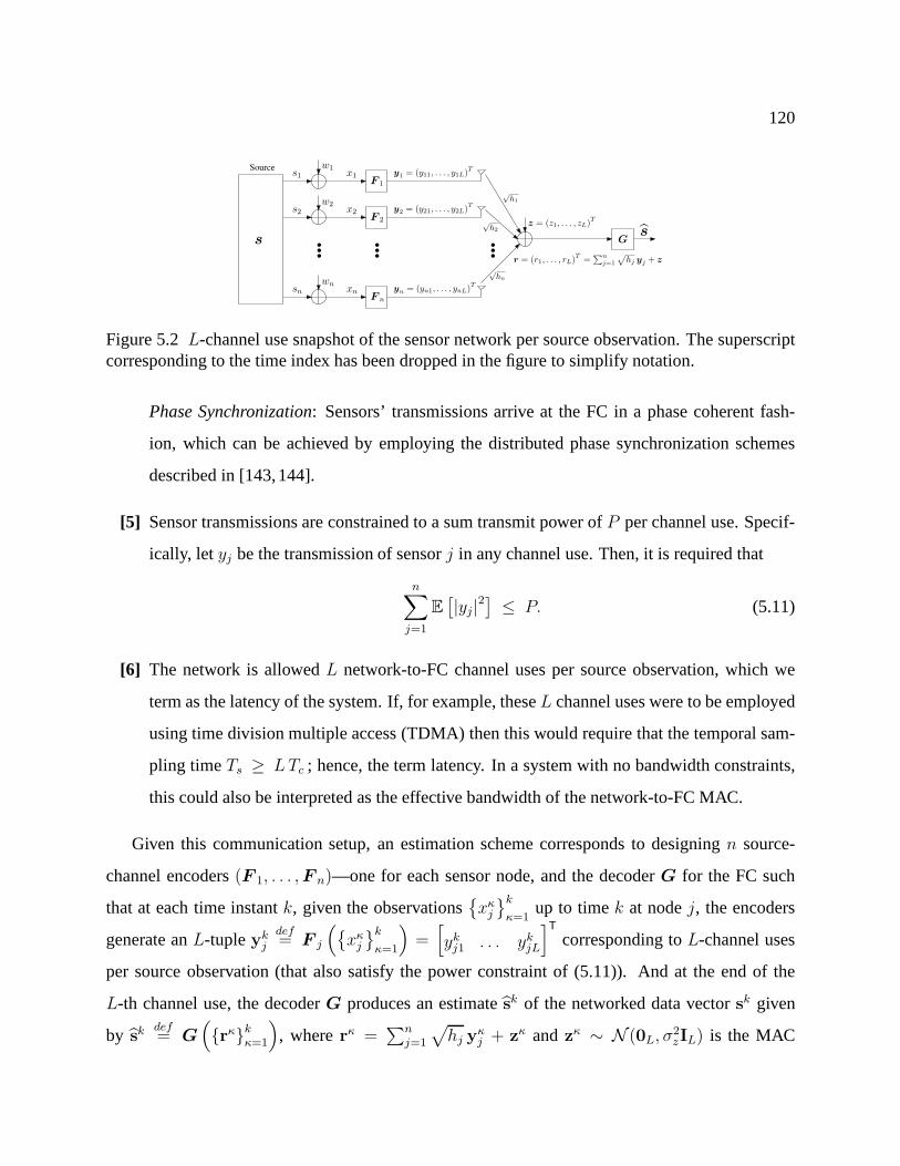
120

... ... ...s

Sources1

s2

sn

w1

w2

wn

x1

x2

xn

F 1

F 2

F n

G

y2

= (y21, . . . , y2L)T

z = (z1, . . . , zL)T

yn = (yn1, . . . , ynL)T

y1

= (y11, . . . , y1L)T

s

r = (r1, . . . , rL)T

=∑n

j=1

√hj yj + z

√

h1

√

h2

√

hn

Figure 5.2L-channel use snapshot of the sensor network per source observation. The superscriptcorresponding to the time index has been dropped in the figureto simplify notation.

Phase Synchronization: Sensors’ transmissions arrive at the FC in a phase coherentfash-

ion, which can be achieved by employing the distributed phase synchronization schemes

described in [143,144].

[5] Sensor transmissions are constrained to a sum transmit power of P per channel use. Specif-

ically, let yj be the transmission of sensorj in any channel use. Then, it is required that

n∑

j=1

E[|yj|2

]≤ P. (5.11)

[6] The network is allowedL network-to-FC channel uses per source observation, which we

term as the latency of the system. If, for example, theseL channel uses were to be employed

using time division multiple access (TDMA) then this would require that the temporal sam-

pling timeTs ≥ LTc ; hence, the term latency. In a system with no bandwidth constraints,

this could also be interpreted as the effective bandwidth ofthe network-to-FC MAC.

Given this communication setup, an estimation scheme corresponds to designingn source-

channel encoders(F 1, . . . ,F n)—one for each sensor node, and the decoderG for the FC such

that at each time instantk, given the observationsxκ

j

k

κ=1up to timek at nodej, the encoders

generate anL-tupleykj

def= F j

(xκ

j

k

κ=1

)=[yk

j1 . . . ykjL

]Tcorresponding toL-channel uses

per source observation (that also satisfy the power constraint of (5.11)). And at the end of the

L-th channel use, the decoderG produces an estimatesk of the networked data vectorsk given

by sk def= G

(rκk

κ=1

), whererκ =

∑nj=1

√hj yκ

j + zκ andzκ ∼ N (0L, σ2zIL) is the MAC

121

AWGN vector corresponding to theL-channel uses at time instantκ (see Figure 5.2), and the goal

of the sensor network is to minimize (i) the average total network power consumption per source

observation

Ptotdef= lim

K→∞

1

K

K∑

k=1

L∑

ℓ=1

n∑

j=1

E

[∣∣ykjℓ

∣∣2]; (5.12)

(ii) the mean-squared error distortion measure

Ddef= lim

K→∞

1

K

K∑

k=1

E

[1

n

∥∥sk − sk∥∥2

2

]; (5.13)

and (iii) the latencyL (# of channel uses per source observation) of the system.3 Thus, for a

fixed number of sensor nodesn, the performance of any estimation scheme is characterizedby the

triplet (Ptot(n), D(n), L(n)) and rather than obtaining an exact expression for this triplet, our goal

would be to analyze how do these three quantities scale withn for a given scheme. Moreover,

minimization of all three quantities in the triplet is sometimes a conflicting requirement and there

is often a trade-off involved between minimizingPtot,D andL, and we shall also be analyzing this

power-distortion-latency trade-off as a function ofn.

Remark 5.6 Notice that implicit in this formulation is the fact that no collaboration among the

sensor nodes is allowed for the purposes of signal estimation, i.e., encoderF j does not have access

to the inputs of any sensor other than sensorj.

Remark 5.7 Note that while stating the performance metrics of power andlatency, we have ig-

nored the cost of initializing the sensor network (primarily corresponding to the cost of channel

gain estimation/phase synchronization algorithms under the current communication setup and the

cost of initial route/topology discovery algorithms underthe more traditional multi-hop commu-

nication setups). This is because the average cost of this initialization (over time) tends to zero as

k—the time scale of the network operation—tends to infinity. Of course, in practice, a one-time

initialization may not suffice and these procedures may haveto be repeated from time to time, but

3Notice that with the distortion metric as defined in (5.13), the MSE of any arbitrary length signal can at worst be

a constant sincelimK→∞

1

K

∑K

k=1E

[1

n

∥∥sk∥∥2

2

]≤ B2.

122

we will assume that the corresponding costs are negligible compared to the routine sensing and

communication operations.

5.3 Optimal Distortion Scaling in a Centralized System

In this section, we consider a system in which the sensor measurementsxk

j

n

j=1at each time

instantk are assumed to be available at the FC with no added cost or noise due to communications,

and we review the corresponding classical estimation theory results (see, e.g., [123,131,145]). Note

that such a system corresponds to a sensor network with a noise-free network-to-FC MAC and thus,

the optimal distortion scaling achievable under thiscentralizedsetting serves as a benchmark for

assessing the distortion related performance of any schemeunder the original setup.

5.3.1 Compressible Signals

Given the observation vectorxk at the FC, an optimal centralized estimator for anα-compress-

ible signal can be easily constructed by projectingxk onto them basis vectors ofΨ corresponding

tom largest (in the absolute sense)Ψ -coefficients ofsk (see, e.g., [131]), i.e., ifΨkm is then ×m

matrix of those basis vectors, where the superscriptk indicates that the re-indexing in (5.3) may be

a function of the time indexk, thensk can be estimated as

skcen

def= Ψ k

m

(Ψk

m

Txk)

= sk,(m) + Ψkm

(Ψ k

m

Twk)

(5.14)

which results in

E

[1

n

∥∥sk − skcen

∥∥2

2

]=

1

n

∥∥sk − sk,(m)∥∥2

2+

1

nE

[∥∥∥Ψ km

(Ψ k

m

Twk)∥∥∥

2

2

](5.15)

≤ Com−2α +

(mn

)σ2

w . (5.16)

Furthermore, from (5.15), we also have the trivial lower bound of

E

[1

n

∥∥sk − skcen

∥∥2

2

]≥ 1

nE

[∥∥∥Ψkm

(Ψ k

m

Twk)∥∥∥

2

2

]=(mn

)σ2

w (5.17)

and combining the upper and lower bounds of (5.16) and (5.17), we obtain(mn

)σ2

w ≤ E

[1

n

∥∥sk − skcen

∥∥2

2

]≤ Com

−2α +(mn

)σ2

w . (5.18)

123

From this expression, we see that the choice ofm affects the classic bias-variance trade-off [145]:

increasingm causes the boundCom−2α on the approximation error1

n

∥∥sk − sk,(m)∥∥2

2(the squared

“bias”) to decrease, but causes the stochastic component ofthe error due to the measurement noise

1n

E

[∥∥∥Ψ km

(Ψk

m

Twk)∥∥∥

2

2

]=(

mn

)σ2

w (the “variance”) to increase. The upper bound is tight, in

the sense that there exist signals for which the upper bound is achieved, and in such cases the

upper bound is minimized (by choice ofm) by making the approximation error and the stochastic

component of the error scale at the same rate, i.e.,

m−2α ≍ m

n⇐⇒ m ≍ n1/(2α+1) (5.19)

resulting in the following expression for optimal distortion scaling of anα-compressible signal in

a centralized system4

D∗cen = lim

K→∞

1

K

K∑

k=1

E

[1

n

∥∥sk − skcen

∥∥2

2

]≍ n−2α/(2α+1). (5.20)

5.3.2 Sparse Signals

Similar to a compressible signal, an optimal centralized estimator for anM-sparse signal cor-

responds to projecting the observation vector onto theM basis vectors ofΨ corresponding toM

nonzeroΨ -coefficients ofsk (see, e.g., [123]), i.e., ifΨ kM is then × M matrix of those basis

vectors, thensk can be estimated as

skcen

def= Ψk

M

(Ψk

M

Txk)

= sk + Ψ kM

(Ψ k

M

Twk)

(5.21)

which results in the usual parametric rate

E

[1

n

∥∥sk − skcen

∥∥2

2

]=

1

nE

[∥∥∥Ψ kM

(Ψk

M

Twk)∥∥∥

2

2

]=

(M

n

)σ2

w (5.22)

resulting in the following expression for optimal distortion scaling of anM-sparse signal in a

centralized system

D∗cen =

(M

n

)σ2

w ≍ M

n. (5.23)

4∗ in D∗

cen refers to the fact that this is theoptimalcentralized distortion scaling.

124

Note that it might very well be thatM—the number of degrees of freedom (DoF) of anM-sparse

signal—scales with the number of nodesn in the network. For example, two-dimensional piece-

wise constant fields with one-dimensional boundaries separating constant regions can be com-

pressed using the discrete wavelet transform and haveM ≍ n1/2 log(n) nonzero wavelet coeffi-

cients [146]. Therefore, we modelM asM ≍ nµ, where0 ≤ µ < 1 and hence, the inclusion of

M in the scaling relation in (5.23).

Remark 5.8 Note that the optimal distortion scaling relations of (5.20) and (5.23) for compress-

ible and sparse signals have been obtained under the assumption that the FC has precise knowledge

of the ordering of coefficients ofsk in the compressing basis (indices of nonzero coefficients ofsk

in the sparse basis). This is not necessarily a problem in a centralized setting and in cases where

this information is not available, coefficient thresholding methods can be used to automatically

select the appropriate basis elements from the noisy data, and these methods obey error bounds

that are within a constant or logarithmic factor of the ones given above (see, e.g., [147,148]).

5.4 Distributed Projections in Wireless Sensor Networks

In this section, we develop the basic communication architecture that acts as a building block of

our proposed estimation scheme. As evident from the previous section, each DoF of a compressible

or sparse signal corresponds to projection of networked data onto ann-dimensional vector inRn

and at the heart of our approach is a distributed method of communicating such projections to the

FC in a power efficient manner by exploiting the spatial averaging inherent in an AWGN MAC.

To begin, assume that the goal of the sensor network is to obtain an estimate of the projection

of networked data, corresponding to each observation of thephysical phenomenon, onto a vector

in Rn at the FC. That is, let us suppose that at each time instantk, we are interested in obtaining

an estimateυk of

υk def= ϕTsk =

n∑

j=1

ϕjskj (5.24)

whereϕ ∈ Rn. One possibility for realizing this goal is to nominate a clusterhead in the net-

work and then, assuming all the sensor nodes know their respective ϕj ’s and have constructed

125

routes which form a spanning tree through the network to the clusterhead, each sensor node can

locally computeϕjxkj = ϕj(s

kj + wk

j ) and these values can be aggregated up the tree to obtain

υk =∑n

j=1 ϕjxkj at the clusterhead, which can then encode and transmit this estimate to the FC.

However, even if we ignore the communication cost of delivering υk from the clusterhead to the

FC, it is easy to check that such a scheme requires at leastn transmissions. For a similar reason,

gossip algorithms such as the ones described in [149, 150], while known for their robustness in

the face of changing network topology, might not be the schemes of first choice for these types of

applications.

Another, more promising, alternative is to exploit recent results concerning uncoded (analog)

coherent transmission schemes in WSNs [40–43]. The proposed distributed joint source-channel

communication architecture requires only one channel use per source observation (Lυ = 1) and is

based on the notion of so-called “matched source-channel communication” [42, 43]: the structure

of the network communication architecture should “match” the structure of the optimal estimator.

Under the current setup, this essentially involves phase-coherent, low-power, analog transmission

of appropriately weighted sample values directly from the nodes in the network to the FC via the

AWGN network-to-FC MAC and the required projection is implicitly computed at the FC as a

result of the spatial averaging in the MAC. In light of the communication setup of Section 5.2, full

characterization of this architecture essentially entails characterization of the correspondingscalar-

output source-channel encoders(F1, . . . , Fn) at the sensor nodes and thescalar-inputdecoder

G at the FC, where scalar nature of the encoders and the decoderis owing to the fact that (by

construction)Lυ = 1 in this scenario.

To begin with, each sensor encoderFj in this architecture corresponds to simply multiplying

the sensor measurementxkj with

(√ρhjϕj

)to obtain5

ykj

def= Fj

(xκ

j

k

κ=1

)=

√ρ

hjϕjx

kj , j = 1, . . . , n (5.25)

whereρ > 0 is a scaling factor used to satisfy sensors’ sum transmit power constraintP , and all

the nodes coherently transmit their respectiveykj ’s in an analog fashion over the network-to-FC

5Practical schemes of how each sensor encoder might get access to its respectiveϕj is discussed in Section 5.5.3.

126

MAC. Under the synchronization assumption of Section 5.2 and the additive nature of an AWGN

MAC, the corresponding received signal at the FC is given by

rk =n∑

j=1

√hj y

kj + zk =

√ρ

n∑

j=1

ϕjxkj + zk

=√ρ υk +

(√ρ ϕTwk + zk

)(5.26)

wherezk ∼ N (0, σ2z) is the MAC AWGN at timek (independent ofwk). In essence, the encoders

(F1, . . . , Fn) correspond to delivering to the FC a noisy projection ofsk ontoϕ that is scaled by√ρ [cf. (5.26)]. Givenrk, the decoderG corresponds to a simple re-scaling of the received signal

υk def= G

(rκk

κ=1

)=

rk

√ρ

= υk +ϕTwk +zk

√ρ. (5.27)

We are now ready to characterize the power-distortion-latency triplet (Ptot,υ , Dυ , Lυ) of the pro-

posed joint source-channel communication architecture for computing distributed projections of

networked data.6

Theorem 5.9 Letϕ ∈ Rn and letυk = ϕTsk. Given the sensor network model of Section 5.2, the

joint source-channel communication scheme described by the encoders in (5.25) and the decoder

in (5.27) can achieve the following end-to-end distortion by employing only one channel use per

source observation

Dυdef= lim

K→∞

1

K

K∑

k=1

E

[∣∣υk − υk∣∣2]

= σ2w ‖ϕ‖2

2 +

(σ2

z duζ (B2 + σ2

w)

λP

)‖ϕ‖2

2 (5.28)

whereυk is the estimate ofυk at the FC,σ2w is the measurement noise variance,σ2

z is the channel

noise variance,B is the bound on|skj |, du is the bound on the maximum distance between the

sensor nodes and the FC,ζ is the path-loss exponent,P is the sum transmit power constraint per

6(Ptot,υ , Dυ , Lυ) triplet here corresponds to power, distortion, and latencyof the projection coefficient as opposedto (Ptot, D, L) in Section 5.2 that corresponds to power, distortion, and latency required to estimate the entire signal.

127

channel use, andλ = λ(n) ∈ (0, 1] is a design parameter used to control total network power

consumption. Moreover, the total network power consumption per source observation associated

with achieving this distortion is given by

λP

(σ2

w

duζ (B2 + σ2

w)

)≤ Ptot,υ

def= lim

K→∞

1

K

K∑

k=1

n∑

j=1

E

[∣∣ykj

∣∣2]≤ λP. (5.29)

Proof: To establish this theorem, first observe that (5.27) impliesthat∀ k ∈ N

E

[∣∣υk − υk∣∣2]

= E

[∣∣∣∣ϕTwk +

zk

√ρ

∣∣∣∣2]

= σ2w ‖ϕ‖2

2 +σ2

z

ρ(5.30)

resulting in the following expression for the projection coefficient MSE

Dυ = σ2w ‖ϕ‖2

2 +σ2

z

ρ. (5.31)

As for obtaining an expression forPtot,υ , note that (5.25) implies that∀ k ∈ N,

ρ σ2w

n∑

j=1

|ϕj|2 ≤n∑

j=1

E

[∣∣ykj

∣∣2]

=n∑

j=1

E

[ρ

hj

(sk

j + wkj

)2 |ϕj|2]

≤ ρ duζ(B2 + σ2

w

) n∑

j=1

|ϕj|2 (5.32)

and, therefore,

ρ = λP

(1

duζ (B2 + σ2

w) ‖ϕ‖22

)(5.33)

would suffice to satisfy the sum transmit power constraint of(5.11), whereλ = λ(n) ∈ (0, 1]

is a power scaling factor to be used by the designer of a WSN to control total network power

consumption. This in turn results in the following expression for total network power consumption

per source observation

λP

(σ2

w

duζ (B2 + σ2

w)

)≤ Ptot,υ ≤ λP. (5.34)

128

Finally, substituting the value ofρ from (5.33) in (5.31) yields (5.28), thereby completing theproof

of the theorem.

Notice that the projection coefficient distortionDυ achieved by the proposed joint source-

channel communication architecture has been expressed in terms of two separate contributions

[cf. (5.28), (5.31)], the first of which is independent of theproposed communication scheme. This

term is solely due to the noisy observation process (σ2w 6= 0) and scales like‖ϕ‖2

2. The second

contribution is primarily due to the noisy communication channel and scales like‖ϕ‖22/λ. More-

over, given the observation model of Section 5.2, it is easy to check thatD∗υ ≍ ‖ϕ‖2

2 is the best

that any (centralized or distributed) scheme can hope to achieve in terms of an order relation for

distortion scaling [123]. Therefore, for optimal distortion scaling, it is sufficient that the second

term in (5.31) also scales like‖ϕ‖22 and hence,λ = O(1) would suffice to ensure that

Dυ ≍ ‖ϕ‖22 ≍ D∗

υ . (5.35)

Consequently, the total network power consumption associated with achieving this optimal distor-

tion scaling would be given byPtot,υ = O (1) [cf. (5.34)]. We summarize this insight as follows.

Corollary 5.10 Let ϕ ∈ Rn and letυk = ϕTsk. Given the sensor network model of Section 5.2

and assuming that the system parameters(B, σ2w, σ

2z , du, ζ, P ) do not vary with the number of nodes

n in the network, the joint source-channel communication scheme described by the encoders in

(5.25) and the decoder in (5.27) can obtain an estimateυk of υk at the FC, such thatDυ ≍ ‖ϕ‖22 ≍

D∗υ , by employing only one channel use per source observation,Lυ = 1, and using a fixed amount

of total network power,Ptot,υ = O (1).

Observation 1 While the original problem has been setup under afixedsum transmit power con-

straintP , one of the significant implications of the preceding analysis is that even if one allows

P to grow with the number of nodes in the network—say, e.g.,P = O(n)—one cannot improve

on the distortion scaling law ofO (‖ϕ‖22). In other words, when it comes to estimating a single

projection coefficient in the presence of noise, using more than a fixed amount of total power per

channel use is wasteful as the distortion due to the measurement noise (first term in (5.31)) is the

limiting factor in the overall distortion scaling.

129

Observation 2 Even though the joint source-channel communication architecture described in

this section is meant to be a building block for the signal estimation scheme, the architecture is

important in its own right too. Often times, for example, rather than obtaining an estimate of the

networked data at the FC, the designer of a WSN is merely interested in obtaining the estimates of

a few of its linear summary statistics. And, given that any linear summary statistic is nothing but

the projection of networked data onto a vector inRn, preceding analysis implies that one can obtain

such linear summary statistics at the FC with minimal distortion (and latency) and consumption of

only a small amount of total network power.

Example 5.11 (Networked Data Average)To illustrate this idea further, consider a specific case

where the designer of a WSN is interested in obtaining an estimate of the averagesk = 1n

∑nj=1 s

kj

of networked data at each time instantk. This would correspond to the projection vector being

given byϕ =[1/n . . . 1/n

]Tand thus, using the communication architecture described in this

section, an estimate ofsk can be obtained at the FC such thatDs ≍ 1/n ≍ D∗s (the parametric

rate),Ls = 1, andPtot,s = O (1).

5.5 Distributed Estimation from Noisy Projections: Known Subspace

In this section, we build upon the joint source-channel communication architecture of Sec-

tion 5.4 and using it as a basic building block, present a completely decentralized scheme for

efficient estimation of networked data at the FC. The analysis in this section is carried out under

the assumption that the designer of the WSN has complete knowledge of the basis in whichS

is compressible (or sparse) as well as precise knowledge of the ordering of its coefficients in the

compressing basis (indices of nonzero coefficients in the sparse basis) at each time instantk. We

refer to this scenario as theknown subspacecase and, under this assumption, analyze the corre-

sponding power-distortion-latency scaling laws of the proposed scheme as a function of number

of sensor nodes in the network. As to the question of whether the known subspace assumption is

a reasonable one, the answer depends entirely on the underlying physical phenomenon. For exam-

ple, if the signal is smooth or bandlimited, then the Fourieror wavelet coefficients can be ordered

(or partially ordered) from low frequency/resolution to high frequency/resolution. Alternatively, if

130

the physical phenomenon under observation happened to be spatially Holder smooth at each time

instantk, then it would be quite reasonable to treat the resulting networked data under the known

subspace category (see, e.g., [43,151]).

5.5.1 Estimation of Compressible Signals

To begin with, letΨ = ψini=1 be the compressing basis ofS such that1

n

∥∥sk − sk,(m)∥∥2

2=

O(m−2α) ∀ k ∈ N. In Section 5.4, we showed that using the communication scheme described

by the encoders in (5.25) and the decoder in (5.27), one projection per snapshot can be efficiently

communicated to the FC by employing only one channel use (Lυ = 1). By a simple extension of

the encoders/decoder structure of Section 5.4, however, the network can equally well communicate

L (> 1) projections per snapshot inL consecutive channel uses (one channel useper projection

per snapshot). Essentially, at each time instantk, theL-tuples generated by the encodersF j are

given by (cf. Section 5.2, Figure 5.2)

ykj = F j

(xκ

j

k

κ=1

)=[yk

j1 . . . ykjL

]T

=

√ρ

hj

[ψ1j x

kj . . . ψLj x

kj

]T, j = 1, . . . , n (5.36)

whereρ = (λP )/(duζ(B2 +σ2

w)), and at the end of theL-th channel use, the received signal at the

input of the decoderG is given by

rk =n∑

j=1

√hj yk

j + zk

=√ρ[∑n

j=1 ψ1j xkj . . .

∑nj=1 ψLj x

kj

]T+ zk

=√ρθk

L +(√

ρΨkL

Twk + zk

)(5.37)

whereΨ kL is then × L matrix of the basis vectors corresponding toL largest (in magnitude)Ψ -

coefficients ofsk, θkL

def=[θk1 . . . θk

L

]T= Ψk

L

Tsk andzk ∼ N (0L, σ

2zIL) is the MAC AWGN

vector (independent ofwk). Thus, at the end of theL-th channel use, the decoder has access toL

scaled, noisy projections ofsk ontoL distinct elements ofΨ and, using these noisy projections, it

131

produces an estimate of the networked data vectorsk given by

sk = G(rκk

κ=1

)= Ψ k

L

(rk

√ρ

)

= sk,(L) + Ψ kL

(Ψ k

L

Twk)

+Ψ k

L zk

√ρ

. (5.38)

Notice the intuitively pleasing similarity betweensk andskcen [cf. (5.14), (5.38)]: the first two terms

in the above expression correspond identically to the centralized estimate of a compressible signal

(with m replaced byL) and the last term is introduced due to the noisy MAC communication. In

particular, this results in the following expression for distortion of a compressible signal at the FC

(L

n

)σ2

w +

(L

n

)(σ2

z duζ (B2 + σ2

w)

λP

)≤ D ≤ Co L

−2α +

+

(L

n

)σ2

w +

(L

n

)(σ2

z duζ (B2 + σ2

w)

λP

). (5.39)

Finally, simple manipulations along the lines of the ones inSection 5.4 result in the following

expression for total network power consumption

λLP

(σ2

w

duζ (B2 + σ2

w)

)≤ Ptot ≤ λLP. (5.40)

The above two expressions essentially govern the interplaybetweenPtot,D, andL of the proposed

distributed estimation scheme and we shall analyze this interplay in further details in the sequel.

Minimum Power and Latency for Optimal Distortion Scaling

Similar to the case of distortion scaling in the centralizedsetting, (5.39) shows that the choice

of number of projections per snapshot in the distributed setting also results in a bias-variance

trade-off: increasingL causes the boundCo L−2α on the approximation error1

n

∥∥sk − sk,(L)∥∥2

2

to decrease, but causes the stochastic components of the error due to the measurement noise

1n

E

[∥∥∥Ψ kL

(Ψ k

L

Twk)∥∥∥

2

2

]=(

Ln

)σ2

w and the communication noise1n

E

[∥∥Ψ kL zk/

√ρ∥∥2

2

]=(

Ln

)·

(σ2

z duζ(B2+σ2

w)λP

)to increase. Consequently, the tightest upper bound scaling in (5.39) is attained

by making the approximation error, the measurement noise error, and the communication noise

132

error scale (as a function ofn) at the same rate. That is, assuming that the system parameters

(Co, B, σ2w, σ

2z , du, ζ, P ) do not depend onn,

L−2α ≍ L

n≍ L

λn(5.41)

implying thatL must be chosen, independently ofλ, as

L ≍ n1/(2α+1) (5.42)

which in turn requires thatλ = O(1), resulting in the following expression for optimal distortion

scaling

D∗ ≍ L−2α ≍ n−2α/(2α+1) (5.43)

that has the same scaling behavior as that ofD∗cen [cf. (5.20)]. Moreover, the total network power

consumption associated with achieving this optimal distortion scaling is given by [see (5.40)]

Ptot ≍ L ≍ n1/(2α+1). (5.44)

Combining (5.42), (5.43), and (5.44), we can also compactlycharacterize the relationship between

optimal distortion scaling and the associated power and latency requirements in terms of the fol-

lowing expression

D∗ ∼ Ptot−2α ∼ L−2α. (5.45)

Note that this expression does not mean that a WSN with fixed number of sensor nodes using

more power and/or latency can provide better accuracy. Rather, power, distortion, and latency

are functions of the number of nodes and the above relation indicates how the three performance

metrics behave with respect to each other as the density of nodes increases.

Remark 5.12 Equation (5.44) shows that the total network power requirement of our proposed

scheme for optimal distortion scaling(D∗ ≍ n−2α/(2α+1)) is given byPtot ≍ n1/(2α+1). A natural

question is:How good is this scheme in terms of power scaling?While a comparison with all

conceivable schemes does not seem possible, in order to givean idea of the performance of our

133

proposed scheme we compare it to a setup where all the nodes inthe network noiselessly commu-

nicate their measurements to a designated cluster of1 ≤ n ≤ n nodes. Each node in the cluster

computes the requiredL projections of the measurement data for each snapshot and then all the

n nodes coherently transmit these (identical) projections to the FC over the MAC; in this case,

the n × 1 MAC is effectively transformed into a point-to-point AWGN channel with ann-fold

power-pooling (beamforming) gain. One extreme,n = 1, corresponds to a single clusterhead

(no beamforming gain), whereas the other extreme,n = n, corresponds to maximum beamform-

ing gain. Note that in our proposed scheme, nodes transmit coherently (and hence benefit from

power-pooling) but there is no data exchange between them. An exact comparison of our scheme

with the above setup involving in-network data exchange is beyond the scope of this exposition

since quantifying the cost of required in-network communication is challenging and requires mak-

ing additional assumptions. Thus, we ignore the cost of in-network communication and provide a

comparison just based on the cost of communicating the projections to the FC—though, in general,

we expect the in-network cost to increase with the sizen of the cluster. Under this assumption, the

analysis in Section 5.10.1 shows that our scheme requires less communication power compared

to the n = 1 case, whereas it requires more power compared to then = n case. In particular,

the power scaling achieved by our proposed scheme (for optimal distortion scaling) is identical

to that in the case when there aren = nL≍ n2α/(2α+1) nodes in the designated cluster to coher-

ently communicate the requiredL ≍ n1/(2α+1) projection coefficients to the FC. Note that since

n2α/(2α+1) ր n for highly compressible signals(α ≫ 1), the performance of our proposed esti-

mation scheme in this case approaches that of then = n extreme, without incurring any overhead

of in-network communication.

Power-Distortion-Latency Scaling Laws for Consistent Estimation

Preceding analysis shows that in order to achieve the optimal centralized distortion scaling

n−2α/(2α+1), the network must expend powerPtot and incur latencyL that scale (withn) at a

sublinear rate ofn1/(2α+1). This may pose a bottleneck in deploying dense WSNs for certain types

of applications that might require extended battery life orfaster temporal sampling of the physical

134

phenomenon. Cursory analysis of (5.39) and (5.40), however, shows that it is possible to lower

these power and latency requirements at the expense ofsub-optimaldistortion scaling, and in the

sequel, we shall be analyzing these power-distortion-latency scaling regimes.

Notice that under the assumption of system parameters(Co, B, σ2w, σ

2z , du, ζ, P ) not varying

with n, L andλ are the only two quantities that bear upon the required network power and achiev-

able distortion of the estimation scheme [see (5.39), (5.40)]. Therefore, we begin by treatingL

(effective number of projections per snapshot) as an independent variable and model its scaling

behavior asL ≍ nβ for β ∈ (0, 1), while we model the scaling behavior ofλ asλ ≍ n−δ for

δ ∈ [0,∞) (recall, 0 < λ ≤ 1).7 Note thatβ = β∗ def= 1/(2α + 1) has already been solved

previously (resulting inδ = δ∗def= 0) and corresponds to the optimal distortion scaling of (5.43).

Bias-Limited Regime. Recall thatL ≍ n1/(2α+1) is the critical scaling of the number of pro-

jections at which point the distortion component due to the approximation error scales at the same

rate as the distortion component due to the measurement noise [cf. (5.41), (5.42)]. If, however, we

let L (≍ nβ) scale at a rate such thatβ < β∗, then the first term in the upper bound in (5.39) that

is due to the approximation error (bias term) starts to dominate the second term that is due to the

measurement noise and, ignoring constants, the resulting distortion at the FC scales as

n−1+β+δ D n−2αβ + n−1+β+δ (5.46)

and the corresponding choice ofoptimalδ is given by

δ = 1 − (2α+ 1)β (5.47)

where optimal here refers to the fact that (i)δ < 1−(2α+1)β is wasteful of power since distortion

component due to the approximation error (first term in the upper bound in (5.46)) in that case

decays slower than the distortion component to the communication noise (second term in the upper

bound in (5.46)), and (ii)δ > 1−(2α+1)β is wasteful of projections (i.e., latency) since distortion

component due to the approximation error in that case decaysfaster than the distortion component

7There is nothing particular about choosingL as the independent variable except that it makes the analysis slightlyeasier. Nevertheless, we might as well start off by treatingλ as the independent variable and reach exactly the sameconclusions.

135

due to the communication noise. With this balancing ofL andλ, distortion goes to zero at the rate

D ≍ n−2αβ (5.48)

as long as the chosenβ ∈(0, 1/(2α+1)

), and the corresponding total network power consumption

is given by [cf. (5.40)]

Ptot ≍ n(2α+2)β−1 (5.49)

resulting in the following expression for power-distortion-latency scaling relationship in the bias-

limited regime

D ∼ Ptot

−2αβ(2α+2)β−1 ∼ L−2α. (5.50)

Variance-Limited Regime. On the other hand, if we letL scale at a rate such thatβ > β∗,

then the second term in the upper bound in (5.39) that is due tothe measurement noise (variance

term) starts to dominate the bias term and the resulting distortion at the FC scales as

D ≍ n−1+β + n−1+β+δ (5.51)

and the corresponding choice of optimalδ is given byδ = 0 (= δ∗). This implies that as long as

the chosenβ ∈(1/(2α+ 1), 1), distortion in the variance-limited regime goes to zero at the rate

D ≍ n−1+β (5.52)

and the corresponding total network power consumption is given by

Ptot ≍ nβ (5.53)

resulting in the following expression for the power-distortion-latency scaling relationship in the

variance-limited regime

D ∼ Ptot− 1

β+1 ∼ L− 1

β+1. (5.54)

Notice that asβ → β∗, both (5.50) and (5.54) collapse to the power-distortion-latency scaling

relationship of (5.45), indicating that the optimal distortion scalingD∗ corresponds to the transition

136

point between the bias-limited and variance-limited regimes. Thus, (5.50) and (5.54) completely

characterize the power-distortion-latency scaling relationship of the proposed distributed estima-

tion scheme for a compressible signal in the known subspace case. This scaling relationship is also

illustrated in Figure 5.3, where the scaling exponents ofPtot andD are plotted againstβ ∈ (0, 1)

(the chosen scaling exponent ofL) for different values ofα.

Observation 3 Analysis of (5.50), (5.54), and Figure 5.3 shows that (i) anydistortion scaling

that is achievable in the variance-limited regime is also achievable in the bias-limited regime,

and (ii) scaling ofPtot in the variance-limited regime is uniformly worse than in the bias-limited

regime. This implies that any WSN observing anα-compressible signal in the known subspace

case should be operated only either in the bias-limited regime or at the optimal distortion scaling

point, i.e.,β ∈ (0, 1/(2α + 1)]. Thus, givenα and a target distortion scaling ofD ≍ n−γ,

0 < γ ≤ 2α/(2α + 1), the number of projections computed by the WSN per snapshot needs to

be scaled asL ≍ nβ , whereβ = γ/2α [cf. (5.50)], and the corresponding total network power

consumption would be given by (5.49). Alternatively, the designer of a WSN could also reverse the

roles ofD andL by specifying a target latency scaling and obtaining the corresponding distortion

(and power) scaling expression.

Observation 4 Another implication of the analysis carried out in this section is that the more

compressible a signal is in a particular basis (i.e., the higher the value ofα), the easier it is to

estimate that signal in the bias-limited regime/at the optimal distortion scaling point (easier in

terms of an improved power-distortion-latency relationship). On the other hand, note that the

power-distortion-latency scaling in the variance-limited regime is completely independent of the

parameterα [cf. (5.54)].

Observation 5 One of the most significant implication of the preceding analysis is that, while

operating in the bias-limited regime, ifβ is chosen to be such thatβ < 1/(2α+2) then the scaling

exponent ofPtot would be negative (cf. (5.49), Figure 5.3). This is remarkable since it shows that,

in principle, consistent signal estimation is possible (D ց 0 asn → ∞) even if the total network

power consumptionPtot goes to zero!

137

0 0.1 0.2 0.3 0.4 0.5 0.6 0.7 0.8 0.9 1−1

−0.8

−0.6

−0.4

−0.2

0

0.2

0.4

0.6

0.8

1

Latency Scaling Exponent (β)

Pow

er &

Dis

tort

ion

Sca

ling

Exp

onen

ts

Pow. Scaling Exp. − α = 1Pow. Scaling Exp. − α = 2Pow. Scaling Exp. − α = 4Dist. Scaling Exp. − α = 1Dist. Scaling Exp. − α = 2Dist. Scaling Exp. − α = 4

Optimal Distortion Scaling Exponents (Correspond to β = 1/(2α + 1))

Power Scaling Exponents Corresponding to Optimal Distortion Scaling

Figure 5.3 Power-distortion-latency scaling relationship of compressible signals in the knownsubspace case. The scaling exponents ofPtot andD are plotted againstβ ∈ (0, 1) for differentvalues ofα. The filled black square on each curve corresponds to the operating point for optimaldistortion scaling (β = β∗), with bias-limited and variance-limited regimes corresponding to thecurve on its left and right side, respectively.

100

101

102

103

104

10−2

10−1

100

Number of Nodes n

Dis

tort

ion

D(n

)

Optimal Dist. ScalingFeasible Dist. ScalingCut−off Dist. Scaling

β Decreasing(from β* to 0)

(a) Different scaling curves forD

100

101

102

103

104

10−4

10−3

10−2

10−1

100

101

Number of Nodes n

Tot

al N

etw

ork

Pow

er P

tot(n

)

Optimal Power ScalingFeasible Power ScalingCut−off Power Scaling

β Decreasing (from β* to 0)

(b) Different scaling curves forPtot

Figure 5.4 Power-Density trade-off for compressible signals in the known subspace case. Variouspower and distortion scaling curves, each one corresponding to a different value ofβ, are plottedon a log-log scale against the number of nodes forα = 1. The dashed curves are the cut-offscalings for consistent signal estimation(β ց 0).

138

Power-Density Trade-off

Viewed in a different way, Observation 5 also reveals a remarkable power-density trade-off

inherent in our approach:increasing the sensor density, while keeping the latency requirements the

same, reduces the total network power consumption requiredto achieve a target distortion level.

This essentially follows from the fact that the power-distortion scaling law in the bias-limited

regime (including the optimal distortion scaling point) follows a conservation relation given by

[cf. (5.48), (5.49)]

PtotD ≍ n2β−1. (5.55)

Specifically, letβ2 < β1 denote two latency scalings in the bias-limited regime and let n2 > n1

denote the corresponding number of nodes needed to achieve atarget distortion levelD(n1, β1) =

D(n2, β2) = Do. Then, we have from (5.48) that

D(n1, β1) = D(n2, β2) ⇒ n−2αβ11 = n−2αβ2

2 (5.56)

and therefore, the corresponding latency requirements arerather trivially related to each other as

L2(n2, β2)

L1(n1, β1)=

nβ2

2

nβ1

1

= 1. (5.57)

Moreover, it follows from (5.55) that the total network power consumptions in the two cases are

related by

Ptot(n2, β2)

Ptot(n1, β1)=

n2β2−12

n2β1−11

=n1

n2

(5.58)

where we have used the fact that (5.56) implies thatn2β1

1 = n2β2

2 . Relations (5.57) and (5.58)

show that increasing the sensor density by a factor ofN , while keeping the number of projections

(per snapshot) communicated by the network to the FC the same, reduces the total network power

required to attain a given target distortion by a factor ofN .

This power-density trade-off is also illustrated in Figure5.4, where various power and distor-

tion scaling curves (corresponding to different values ofβ) are plotted on a log-log scale against

the number of nodes forα = 1. For the sake of illustration, these plots assume that the constants of

139

proportionality in the scaling relations are unity. In order to illustrate the power-density trade-off,

suppose that we want to attain a target distortion ofDo = 0.02. With optimal distortion scaling

(solid curve in Figure 5.4(a) corresponding toβ1 = β∗ = 1/3), the desired distortion can be at-

tained withn1 ≈ 353 nodes, consuming a total network powerPtot(n1, β1) ≈ 7.07, as calculated

from the solid curve in Figure 5.4(b). On the other hand, however, if we operate on a sub-optimal

distortion scaling curve (say, e.g., the third dotted feasible curve from the bottom in Figure 5.4(a)

corresponding toβ2 = 8/33), we would attain the desired distortion ofDo = 0.02 with n2 ≈ 3192

nodes—roughly a factor of 9 increase in sensor density—but would only consume a total network

power ofPtot(n2, , β2) ≈ 0.78, as calculated from the third dotted feasible curve from thetop in

Figure 5.4(b). Thus, as predicted, increasing the sensor density roughly by a factor of 9 reduces

the total network power consumption by a factor of 9, while the latency requirements stay exactly

the same(nβ1

1 = nβ2

2 ).

5.5.2 Estimation of Sparse Signals

The analysis for the estimation of anM-sparse signal in the known subspace case using the

joint source-channel communication architecture of Section 5.4 can be carried out along almost the

same lines as for compressible signals in Section 5.5.1, with the only obvious difference being that

S now lies exactly in anM-dimensional subspace ofRn and therefore,L has to be taken exactly

equal toM , i.e., is no longer a variable parameter in the hands of the designer of a WSN. This

results in the following expressions for the end-to-end distortion at the FC and the corresponding

total network power consumption and system latency

D =

(M

n

)σ2

w +

(M

n

)(σ2

z duζ (B2 + σ2

w)

λP

), (5.59)

λMP

(σ2

w

duζ (B2 + σ2

w)

)≤ Ptot ≤ λMP, (5.60)

L = M. (5.61)

Next, recall that while the scaling behavior ofM is modeled asM ≍ nµ, 0 ≤ µ < 1, the

choice ofµ is not in our hands in this case and, instead, depends upon theunderlying physical

phenomenon. Essentially,µ here plays the role analogous to that ofα in the compressible case.

140

Therefore, unlike the compressible signal case, the only controllable parameter in this case is the

power scaling factorλ, modeled asλ ≍ n−δ for δ ∈ [0,∞), and in the sequel, we analyze the

effect of various scaling behaviors ofλ on the power-distortion-latency scaling relationship of the

proposed estimation scheme.

Power-Distortion-Latency Scaling Laws for Consistent Estimation

We start out by first analyzing the optimal distortion scaling that is achievable for anM-sparse

signal. Notice that for fastest distortion reduction, the first term (due to the measurement noise) in

(5.59) should scale at the same rate as the second term (due tothe communication noise). This in

turn requires thatλ = O(1) (or δ = δ∗def= 0), resulting in the following expression for optimal

distortion scaling

D∗ ≍ M

n≍ n−1+µ (5.62)

which has the same scaling behavior as that ofD∗cen [cf. (5.23)]. Moreover, the total network power

consumption associated with achieving this optimal distortion scaling is given by

Ptot ≍ L = M ≍ nµ. (5.63)

Equations (5.61), (5.62) and (5.63) can also be combined together forµ ∈ (0, 1) to express the rela-

tionship between optimal distortion scaling and the corresponding power and latency requirements

in terms of the following expression

D∗ ∼ Ptot− 1

µ+1 ∼ L− 1

µ+1 . (5.64)

Notice that the above relationship has the same form as that of (5.54) (the power-distortion-latency

relationship of a compressible signal in the variance-limited regime) which is precisely what one

would expect since there is no bias related distortion component for a sparse signal [cf. (5.59)].

Remark 5.13 Equations (5.61), (5.62), and (5.63) show that for the case of µ = 0, i.e.,M = O(1),

optimal distortion scalingD∗ ≍ n−1 can be obtained by consuming only a fixed amount of total

network power and incurring a fixed latency, i.e.,Ptot = L = O(1). This result is similar in spirit

141

to the one obtained in [42] that primarily studies the case analogous to that of a sparse signal with

non-scaling DoF(M = O(1)), albeit assuming Gaussian sources and multiple FCs (see Theorem 1

and Theorem 3 therein).

Power-limited Regime.On the other hand, if we takeδ > 0 then the distortion component due

to the communication noise (second term in (5.59)) starts todominate the distortion component due

to the measurement noise (first term in (5.59)) and, ignoringthe constant parameters, the resulting

distortion at the FC scales as

D ≍ n−1+µ+δ (5.65)

in the power-limited regime. This implies that as long asδ ∈ (0, 1 − µ), distortion can still be

driven to zero, albeit at a slower,sub-optimalrate ofn−1+µ+δ (≻ D∗). In particular, this means

thatD can be asymptotically driven to zero even if the total network powerPtot (≍ nµ−δ) scales

just a little faster thann2µ−1 [cf. (5.60)]. This observation is similar in spirit to the one made for

compressible signals since it shows that, in principle, consistent signal estimation is possible in the

limit of a large number of nodes forµ ∈ [0, 1/2] (i.e., the number of DoFM scaling at most as

fast as√n) even if the total network powerPtot goes to zero. Finally, this power-distortion-latency

scaling relationship in the power-limited regime can be expressed as

D ∼ Ptot−1+µ+δ

µ−δ ∼ L−1+δ

µ+1. (5.66)

Discussion

While quite similar in spirit, there are still some key differences between the power-distortion-

latency scaling laws of the proposed estimation scheme for compressible and sparse signals. To

begin with, unlike for compressible signals, the latency scaling requirements for sparse signals are

dictated by the underlying physical phenomenon(L = M ≍ nµ) and cannot be traded-off for

power and/or distortion without making further assumptions on the decay characteristics of theM

nonzero coefficients ofS. Secondly, the scenario of consistent signal estimation ofsparse signals

with decaying total network power consumption exists if andonly if the number of DoFM scales

142

0 0.1 0.2 0.3 0.4 0.5 0.6 0.7 0.8 0.9 1−1

−0.8

−0.6

−0.4

−0.2

0

0.2

0.4

0.6

0.8

1

Scaling Exponent of M (µ)

Pow

er &

Dis

tort

ion

Sca

ling

Exp

onen

ts

Optimal Pow. ScalingOptimal Dist. ScalingPLR: Feasible Pow.PLR: Feasible Dist.PLR: Cut−off Pow.PLR: Cut−off Dist.

Figure 5.5 Power-distortion-latency scaling relationship of sparse signals in the known subspacecase. The scaling exponents ofPtot andD are plotted against the scaling exponent ofM (≍ nµ) for0 ≤ µ < 1, while the scaling exponent ofL is the same as that ofM . The solid curves correspondto the optimal distortion scaling exponents and the corresponding total network power scalingexponents, while the dotted curves correspond to various power-limited regime (PLR) scalingsthat result in consistent signal estimation. The dashed curves are the cut-off scalings for consistentsignal estimation.

143

at a rate less than or equal to√n, i.e.,µ ≤ 1/2 (see Figure 5.5).8 And finally, as a flip side to this

observation, the power-density trade-off for sparse signals exists only when0 ≤ µ < 1/2, happens

to be a function ofµ, and is not as pronounced for0 < µ < 1/2. Specifically, for an increase in

the sensor density by a factor ofN , the total network power consumption requirements can only

be reduced by a factor ofN1−2µ, 0 ≤ µ < 1/2, in order to attain the same target distortion for a

sparse signal [cf. (5.65)].

5.5.3 Communicating the Projection Vectors to the Network

Recall that an implicit requirement for employing the proposed distributed estimation scheme

in the known subspace case is that the sensor encoders have access to the respective projection

vectors’ elements at each time instantk [cf. (5.36)]. In this subsection, we address the issue of

how one might communicate this information to the sensor nodes. One viable option in this regard

could be the pre-storage of relevant information in each sensor node. However, pre-storage of the

entire compressing (sparse) basisΨ or a subset of it,ψiLi=1, where1 ≤ L ≤ n, in each sensor

node is not feasible in large-scale WSNs since this would require at leastn storage elements per

sensor node. Instead, a better alternative is to store only the correspondingnonzeroelements of

theL projection vectors,ψij : ψij 6= 0Li=1, in the j-th sensor node. In the context of [43], for

example, this would mean having onlyO(1) storage elements per sensor node, since the structure

of the proposed projection vectors in [43] is such that the cardinality of the setψij : ψij 6= 0Li=1

is identically equal to one∀ j = 1, . . . , n. Other instances when pre-storage might be a feasible

option could be, for example, when the projection vectors’ elements come from an analytical

expression. Pre-storage, however, suffers from the drawback that sensor nodes pre-stored with one

compressing (sparse) basis vectors might not be readily deployable in signal fields compressible

(sparse) in some other basis.

Another more feasible, but not always practical, approach to the communication of projection

vectors to the network could be that the FC transmits this information over the FC-to-network8Recall that for compressible signals, this observation holds true for allα.

144

broadcast channel at either the start of the estimation process or at the start of each network-to-

FC channel use. For basisΨ whose vectors have some sort of spatial regularity in their structure

such that they do not require addressing each sensor node individually (e.g., vectors describable

by a few parameters such as in [43]), this could be readily accomplished by broadcasting a few

command signals from the FC to the network. One could also increase the addressing resolution of

the FC by equipping it with multiple transmit antennas and using some of the techniques described

in [152]. However, depending upon the structure of the compressing (sparse) basis, this approach

may require the FC to be able to address each sensor node individually which may or may not be

practical in large-scale dense WSNs. We will show in Section5.6, however, that one benefit of

compressive wireless sensingis a straightforward treatment of this issue.

5.6 Distributed Estimation from Noisy Projections: Unknown Subspace

In Section 5.5, we proposed an efficient distributed estimation scheme that achieves the optimal

centralized distortion scalingD∗cen for both compressible and sparse signals under the assumption

that the WSN has complete knowledge of the basis in whichS is compressible or sparse. Generally

speaking, however, even if the basis in whichS is compressible (sparse) is known, it is quite likely

that the precise ordering of its coefficients (indices of itsnonzero coefficients) in that basis at each

time instantk might not be known ahead of time—a scenario that we refer to asthe unknown

subspaceor adaptive subspacecase. As an example, consider the following simple case. Suppose

S is very sparse in some basisΨ = ψini=1 such that each temporal samplesk has only one

nonzero coefficient of amplitude√nB corresponding tosomeelementψi of Ψ andi is drawn at

random from the set[1 . . . n]. This is an example of the case where we know the basis in whichS

is sparse but do not know the indices of its nonzero coefficients in that basis.

One naıve approach to this problem would be to use the distributed estimation scheme de-

scribed in Section 5.5. However, since the network does not have a precise knowledge of the index

of the true basis vector, it would need to be determined by trial and error (e.g., deterministically

or randomly selecting basis vectors in some fashion). As an illustration, consider a randomized

selection process: the network computes the projection of the sensor data ontoψi andi is selected

145

L times uniformly at random (without replacement) from the set [1 . . . n]. Ignoring the distortion

due to the measurement and communication noise, the squareddistortion error would be 0 at the

FC if the spike in theΨ domain corresponds to one of the uniformly pickedψi’s andB2 otherwise,

and the probability of not finding the spike inL trials is∏L−1

i=0

(1 − 1

n−i

). If n is large enough and

L ≪ n, we can approximate the resulting distortion byD ≈(1 − 1

n

)LB2 ≈ e−L/nB2 → B2 as

n→ ∞, i.e., equivalent to the MSE that is achievable even withoutany information.

Another more general, and perhaps relevant, example is a situation in which the signal field is

spatially piecewise smooth. Signals of this type do lie in a low-dimensional subspace of the wavelet

domain, but precisely which subspace depends on the locations of the change points in the signal,

which of course are unlikely to be known a priori. Broadly speaking, any signal that is generally

spatially smooth apart from some localized sharp changes oredges will essentially lie in a low-

dimensional subspace of a multiresolution basis such as wavelets or curvelets, but the subspace

will be a function of the time indexk and thus, will preclude the use of methods like the one in

Section 5.5 that require prior specification of the basis vectors to be used in the projection process.

This is where theuniversalityof compressive wireless sensing (CWS) scheme, presented inthis

section, comes into play. As we shall see, CWS provides us with a consistent estimation scheme

(Dց0 as node density increases), even if little or no prior knowledge about the networked data is

assumed, whilePtot andL grow at most sub-linearly with the number of nodes in the network.

5.6.1 Compressive Wireless Sensing

Recall that ifυk = ϕTsk =∑n

j=1 ϕjskj is the projection ofsk onto a vectorϕ ∈ Rn then,

using the communication architecture described in Section5.4 and consuming onlyO(1) amount

of power, the FC can obtain an estimate ofυk in one channel use that is given by

υk = υk +ϕTwk + zk (5.67)

wherezk ∼ N (0, σ2z/ρ) is the scaled MAC AWGN [cf. (5.27)]. The basic idea behind CWSis

that instead of projecting the sensor network data onto a subset of a deterministic basis ofRn, the

FC tries to reconstructsk from random projectionsof the sensor network data. Specifically, let

146

φi ∈ Rnni=1 be an i.i.d. sequence of (normalized) Rademacher random vectors, i.e.,φijn

j=1 =

±1/√n, each with probability1/2, and the FC tries to reconstructsk by projectingxk ontoL of

these random vectors.9 Because the entries of each projection vectorφi are generated at random,

observations of this form are called random projections of the signal.

Remark 5.14 An important consequence of using Rademacher random vectors for projection pur-

poses is that each sensor can locally draw the elements of theprojection vectorsφiLi=1 in an

efficient manner by simply using its network address as the seed of a pseudo-random number

generator (see, e.g., [153]). Moreover, given these seed values and the number of nodes in the

network, the FC can also easily reconstruct the vectorsφiLi=1. Therefore, in addition to being

a universal estimation scheme, CWS has an added advantage that no extended information con-

cerning the projection vectors needs to be communicated to (or stored inside) the sensor nodes

(cf. Section 5.5.3).

After employingL random (Rademacher) projections, the corresponding projection estimates

at the FC are simply given by

υki = φT

i sk + φT

i wk + zk

i , i = 1, . . . , L (5.68)

wherewk =[wk

1 . . . wkn

]T, andwk

j nj=1 andzk

i Li=1 are i.i.d. zero-mean Gaussian random

variables, independent of each other andφij, with variancesσ2w andσ2

z/ρ, respectively. The re-

construction process can be described as follows—letSq denote a countable collection of candidate

reconstruction vectors such that

Sq ⊂ y ∈ Rn : |yj| ≤ B, j = 1, . . . , n (5.69)

and define a CWS estimatesk as

sk = arg mins∈Sq

R(s) +

c(s) log(2)

Lǫ

. (5.70)

9The L Rademacher vectors are to be generated independently at each time instantk. However, we omit thesuperscript corresponding to the time index to simplify thenotation.

147

The first term in the objective function is the empirical risk, defined as

R(s)def=

1

L

L∑

i=1

(υk

i − φTi s)2

(5.71)

which measures the average (Euclidean) distance between the observationsυki L

i=1 and the pro-

jections of a given candidate vectors onto the corresponding Rademacher vectorsφiLi=1. The

quantityc(s) in the second term is a non-negative number assigned to each candidate vector in

Sq such that∑

s∈Sq2−c(s) ≤ 1, and is designed to penalize candidate vectors proportional to their

complexity [see (5.76)]. Finally,ǫ > 0 is a constant (independent ofL andn) that controls the

relative contribution of the complexity term to the objective function. In the context of [67, Theo-

rem 1],σ2w = 0 and soǫ depends only the sample boundB and the noise varianceσ2

z/ρ .

In order to apply the results of [67] to the observation model(5.68), the effect of theprojected

noisetermsφTi w

kLi=1 needs to be determined. First, suppose that the projection vectorsφiL

i=1

were mutually orthogonal. In that case, it is easy to see thatthe projected noises are equivalent (in

distribution) to i.i.d. zero-mean Gaussian noises with varianceσ2w. In addition, note thatφT

i wk

andφij are independent. To see this, notice that for any fixed vectorg ∈ Rn, the joint charac-

teristic function ofφTi w

k andφTi g can be factored into the product of the individual characteristic

functions, i.e.,

E

[ejν1φT

i wk+jν2φT

i g]

= E

[ejν1φT

i wk]· E

[ejν2φT

i g], (5.72)

and takingg to be a vector that has one at location ‘j’ and zero at all other locations establishes

the independence ofφTi w

k andφij. In this case, if we pick

ρ =P

duζ (B2 + σ2

w)(5.73)

then the observations in (5.68) would be equivalent (in distribution) to observations of the form

υki = φT

i sk + ηk

i , i = 1, . . . , L, (5.74)

whereηki L

i=1 are i.i.d. zero-mean Gaussian random variables—independentof φij—with vari-

anceσ2 = σ2w + σ2

z duζ (B2 + σ2

w) /P , and the results of [67, Theorem 1] can be applied directly.

148

On the other hand, our model only assumes that the vectorsφiLi=1 are mutually orthogonal

in expectation; hence, the projected noise is colored—ifΦ is theL × n matrix whose rows are

φTi L

i=1 then, givenΦ, the projected noise vectorΦwk is a zero-mean Gaussian vector with co-

variance matrixΦΦTσ2w. Without loss of generality, however, we can assume that theprojected

noiseφTi w

kLi=1 behaves approximately like white Gaussian noise and consequently, use the ob-

servation model of (5.74) for further analysis. This approximation is motivated by the asymptotic

results presented in [8, Section IV-B] which show that the extreme eigenvalues ofΦΦT are al-

most surely (a.s.) contained in the interval[(1 −√

c)2, (1 +

√c)

2]

in the limit asL, n→ ∞ with

L/n→ c. Since we assumeL grows sublinearly withn soL/n→ 0 in our case and consequently,

all the eigenvalues ofΦΦT tend to1 a.s. In other words,φiLi=1 become mutually orthogonal

asymptotically, and the degree of coloring becomes negligible for large values ofn (this approxi-

mation is also shown to work well in practice—see Section 5.8).

Explicit bounds on the reconstruction error using the CWS estimate of (5.70) can then be ob-

tained by first assuming that we can find a basisΨ at the FC in which the signalS isα-compressible

and then, using this compressing basis in the reconstruction process by definingSq and c(s) in

terms ofΨ . Specifically, let

Θqdef=θ ∈ R

n : |(Ψθ)j| ≤ B, θj uniformly quantized tonq levels, j = 1, . . . , n

(5.75)

be a set of quantized candidate solutions in the transform domainΨ , so thatSq = s ∈ Rn : s =

Ψθ, θ ∈ Θq. Furthermore, let the penalty termc(s) = c(θ) be

c(θ)def= (1 + q) log(n)‖θ‖0. (5.76)

Then, the optimization problem (5.70) essentially reducesto solving the problem

θk

= arg minθ∈Θq

∥∥∥υkL −ΦT

LΨθ∥∥∥

2

2+

(1 + q) log(2) log(n)

ǫ‖θ‖0

(5.77)

whereυkL

def=[υk

1 . . . υkL

]T,ΦL is then× L matrix of Rademacher projection vectorsφiL

i=1,

andθk

is the estimate of the representation ofsk in the compressing basisΨ , i.e., sk def= Ψθ

k. As

149

shown in [67], for anα-compressibleS, such an estimate would satisfy10

D (

L

log(n)

)−2α/(2α+1)

(5.78)

while, for anM-sparse signal, this would result in

D (

L

M log(n)

)−1

. (5.79)

5.6.2 Power-Distortion-Latency Scaling Laws

Recall that in order to achieve the distortion scaling of (5.78) and (5.79), the network had to

employL network-to-FC MAC uses per source observation, each one corresponding to a projection

of sk onto a random Rademacher vector. And while the projection vectors in this case happened

to be random as opposed to the analysis carried out in Section5.4, it is a simple exercise to show

that with the scaling factorρ as given in (5.73), each projection of the noisy networked data onto

a (random) Rademacher vector still consumes onlyO(1) amount of power. Therefore, power-

distortion-latency scaling relationship of the CWS schemefor the case whenS is α-compressible

can be given by

D ∼(

Ptot

log(n)

)−2α/(2α+1)

∼(

L

log(n)

)−2α/(2α+1)

(5.80)

while for anM-sparse signal withM andL scaling asM ≍ nµ, 0 ≤ µ < 1, andL ≍ nβ,

0 < β < 1, it can be given by

D ∼ log(n)Ptot−1+ µ

β ∼ log(n)L−1+ µβ . (5.81)

Comparison of these power-distortion-latency relationships with the ones achievable in Sec-

tion 5.5 yields an interesting insight: regardless of the compressibility (sparsity) ofS, if there is

enough prior knowledge about the underlying physical phenomenon, the distortion achievable un-

der CWS would always be greater than the one achievable in theknown subspace case, when using

10The stated results hold for allq ≥ 1; the explicit dependencies of the leading constants on the quantizationparameterq are derived in [67].

150

the same amount of power and latencyand identical reconstruction basis. As an example, whereas

one can obtain a distortion scaling ofD ≍ n−2α/(2α+1) by employing(Ptot ≍)L ≍ n1/(2α+1) pro-

jections for the estimation of anα-compressible signal in the known subspace case, the distortion

scaling in the unknown subspace case, when using the same number of projections can only be

given byD n−2α/(2α+1)2—a significantly slower decay [cf. (5.45), (5.80)].

On the other hand, by virtue of a toy example, we have already seen at the start of this section

what could happen to the distortion scaling in the known subspace case if the known subspace

assumption is false and that is where the universality of CWScomes into play: given sufficient prior

knowledge about the underlying signal field, CWS can be far from optimal but under circumstances

where there islittle or no knowledge available about the signal field, CWS should be thescheme

of choice for estimating compressible or sparse networked data.

5.7 Impact of Fading and Imperfect Phase Synchronization

The joint source-channel communication architecture presented in Section 5.4 for computing

distributed projections in WSNs (and extended to estimation of compressible/sparse signals in

Sections 5.5 and 5.6) is analyzed under the assumptions thatthe network is fully synchronized

and transmissions from the sensor nodes do not undergo fading. This assumption may not hold in

practice for sensor network deployments in scattering environments and due to drifts in phases of

sensor oscillators. Therefore, we relax these assumptionsin this section and study the impact of

fading and imperfect phase synchronization on the previously obtained scaling laws. In particular,

we establish that (i) the power-distortion-latency laws ofSections 5.4 and 5.5 continue to hold as

long as the random channel gains of received signals at the FC(due to fading and phase synchro-

nization errors) have a nonzero mean, and (ii) the CWS scaling laws continue to hold as long as

the mean of these random channel gains is not too small.

5.7.1 Distributed Projections in Wireless Sensor Networks

We begin by analyzing the impact of fading and imperfect phase synchronization on the power-

distortion-latency scaling law of the proposed communication scheme for computing distributed

151

projections (cf. Theorem 5.9). This is accomplished by assuming that the communication scheme

is still described by the encoders in (5.25) but, as a result of narrowband fading and phase syn-

chronization errors, each sensor’s transmitted signal is received at the FC after multiplication by

a random channel gainγkj

def= gk

j cos(∆kj ), j = 1, 2, . . . , n, where the random variablesgk

j and

∆kj are i.i.d. (across sensors), which are also assumed to be independent of each other [21,142].11

Note thatgkj are non-negative valued random variables—typically modeled as Rayleigh, Rician

or log-normal distributed—and correspond to random fadingenvelopes of received signals at the

FC, whereas∆kj model the combined effect of random phase-shifts due to multipath scattering

and imperfect phase synchronization between the sensors and the FC. We assume that the precise

values and distributions of these random variables are not available to the sensors or the FC, but

their means are known at the FC.

Consequently, as a result of fading and imperfect phase synchronization, the FC receives

rk =

n∑

j=1

√hj γ

kj y

kj + zk =

√ρ

n∑

j=1

ϕjγkj x

kj + zk

=√ρ ϕT

(γk ⊙ sk

)+(√

ρ ϕT(γk ⊙wk

)+ zk

)(5.82)

whereγk def=[γk

1 . . . γkn

]T, ⊙ represents a Hadamard product (element-wise multiplication),

andρ is still given by the expression in (5.33). Clearly, this coincides with the received signal in

(5.26) if and only ifγk = 1n, where1n denotes ann-dimensional vector of all ones. However, by

a slight modification of the decoder in (5.27), it can be shownthat the scaling law established in

Theorem 5.10 is still achievable as long as the distributionof random channel gains is such that the

network remains at least “barely synchronized” in the sensethatE[γkj ]

def= γ 6= 0. This condition

would be satisfied, e.g., if∆kj ∼ unif[−π + ǫ, π − ǫ] for anyǫ > 0. The modified decoderG in

this scenario is given by

υk = G(rk)

=rk

γ√ρ

= ϕT(γ

k ⊙ sk)

+ϕT(γ

k ⊙ wk)

+zk

γ√ρ

(5.83)

11Recall that we are doing real-signaling; the random channelgains are, therefore, given byγkj = gk

j cos(∆kj )

instead ofγkj = gk

j ej∆kj .

152

whereγk def=[

γk1

γ. . . γk

n

γ

]T, and the achievable distortion using this modified decoder can be

characterized by the following result.

Theorem 5.15 Letϕ ∈ Rn and letυk = ϕTsk. Suppose that the random channel gainsγkj due

to fading and imperfect phase synchronization are i.i.d across sensors and have a nonzero mean

(E[γkj ] = γ 6= 0).12 Then, given the sensor network model of Section 5.2, the joint source-channel

communication scheme described by the encoders in (5.25) and the modified decoder in (5.83)

can achieve the following end-to-end distortion by employing only one channel use per source

observation

Dυ ≤(σ2

w γ +B2(γ − γ2

)

γ2

)‖ϕ‖2

2 +

(σ2

z duζ (B2 + σ2

w)

λγ2P

)‖ϕ‖2

2 (5.84)

whereυk is the estimate ofυk at the FC andγdef= E[|γk

j |2] ≤ 1 (mainly because of the law of

conservation of energy).

Proof: To establish this theorem, note that (5.83) implies that∀ k ∈ N

E

[∣∣υk − υk∣∣2]

= E

[∣∣∣(ϕT(γ

k ⊙ sk)− ϕTsk

)+ϕT

(γ

k ⊙ wk)

+zk

γ√ρ

∣∣∣2]

(a)= E

[∣∣∣ϕT((γ

k − 1n

)⊙ sk

)∣∣∣2]

+σ2

w γ

γ2 ‖ϕ‖22 +

σ2z

γ2ρ

=

n∑

j=1

(ϕjs

kj

)2E

[(γkj

γ− 1)2]

+σ2

w γ

γ2 ‖ϕ‖22 +

σ2z

γ2ρ

(b)

≤ B2(γ − γ2

)

γ2 ‖ϕ‖22 +

σ2w γ

γ2 ‖ϕ‖22 +

σ2z

γ2ρ(5.85)

where(a) essentially follows from the fact that the random channel gain vectorγk is independent

of the zero-mean measurement noise vectorwk and zero-mean communication noisezk, and(b)

primarily follows from the fact that|skj | ≤ B. Finally, to complete the proof of the theorem, we

substitute in (5.85) the value ofρ from (5.33) and take the limit ink to obtain (5.84).

12At the expense of some extra notation, the scaling laws stated in this section can be obtained even whenγkj are

not identically distributed (as long as they are independent across sensors and have nonzero means). For the sake ofthis exposition, however, and because it suffices to illustrate the principles, we focus only on the i.i.d. case.

153

Remark 5.16 A corresponding lower bound on the projection coefficient distortionDυ under the

modified decoder of (5.83) is given by (5.28). This follows trivially from (a) in (5.85) and the fact

thatγ2 ≤ γ ≤ 1.

Remark 5.17 Since the structure of source-channel encoders(F1, . . . , Fn) remains unchanged

under fading and imperfect phase synchronization, the total network power consumption associated

with achieving the distortion in (5.84) is still given by (5.34).

Notice that even under the effects of fading and imperfect synchronization, the projection co-

efficient distortionDυ achieved by the proposed joint source-channel communication architecture

(using the modified decoder of (5.83)) is given by a sum of two separate terms, the first of which

scales like‖ϕ‖22, while the second term that is primarily due to the noisy communication channel

scales like‖ϕ‖22/λ (cf. (5.84), Remark 5.16). Comparing this observation withthe scaling law

established in Section 5.4 shows that Theorem 5.15 describes the same distortion scaling behavior

as Theorem 5.9, with the only difference being that the scaling constants are now different (they

depend upon the second-order statistics of channel gains).In particular,Lυ = 1 andPtot,υ = O (1)

is still sufficient to ensure thatDυ ≍ ‖ϕ‖22 ≍ D∗

υ, as long asγ 6= 0 (cf. Corollary 5.10).

5.7.2 Distributed Estimation from Noisy Projections: Known Subspace

Similar to the case of estimation of a single projection coefficient under the effects of fading

and imperfect phase synchronization, it is a simple exercise to show that by using the joint source-

channel communication scheme described by the encoders in (5.36) and under a slightly modified

decoderG given by

sk = G(rk) def

= Ψ kL

(rk

γ√ρ

)(5.86)

the end-to-end distortion of anα-compressible signal at the FC in the presence of fading and phase

synchronization errors can be upper bounded by

D ≤ Co L−2α +

(L

n

)(σ2

w γ +B2(γ − γ2

)

γ2

)+

(L

n

)(σ2

z duζ (B2 + σ2

w)

λγ2P

)(5.87)

154

and lower bounded by the expression in the lower bound of (5.39), as long asγkj are i.i.d.

across sensors andγ 6= 0. Ignoring constants, this implies that the resulting distortion of anα-

compressible signal in this scenario still scales as(L

n

)+

(L

λn

) D L−2α +

(L

n

)+

(L

λn

)(5.88)

i.e., has the same scaling behavior as that ofD in (5.39). Similarly, it can be shown that using

the modified decoder of (5.86) (withL replaced byM), the end-to-end distortion of anM-sparse

signal in this scenario would scale as [cf. (5.59)]

D ≍(M

n

)+

(M

λn

). (5.89)

Moreover, given that the structure of source-channel encoders(F 1, . . . ,F n) remains unchanged

under fading and imperfect phase synchronization, the total network power consumption per source

observation associated with achieving these distortion scalings for compressible and sparse signals

would still be given by (5.40) and (5.60), respectively. Comparison of these results with the ones

obtained in Section 5.5 shows that the previously established power-distortion-latency scaling laws

for estimation of compressible and sparse signals in the known subspace case continue to hold

under the effects of fading and imperfect phase synchronization, providedγkj have a nonzero

mean and the FC uses the modified decoder of (5.86).

Remark 5.18 Note that these results are similar in spirit to some of the earlier results obtained

in the context of joint source-channel communication for distributed estimation of sources—see,

e.g., [42,154–156]. In particular, those results also indicate that fading (and/or imperfect synchro-

nization) tends to have no effect on the distortion scaling as long as the random channel gains have

nonzero means.

5.7.3 Compressive Wireless Sensing

In the presence of phase synchronization errors only (no fading, i.e.,γkj = cos(∆k

j ) only), CWS

observations are given by(∀ i = 1, . . . , L)

υki = φT

i

(γ

k ⊙ sk)

+ φTi

(γ

k ⊙ wk)

+zk

i

γ√ρ

(5.90)

155

whereγk =[

γk1

γ. . . γk

n

γ

]T[see (5.68)]. Defining the vectorγk asγk def

= 1n+δk and substituting

into the above gives

υki = φT

i sk + φT

i wk + φT

i

(δk ⊙ (sk + wk)

)+

zki

γ√ρ

(5.91)

whereδk is a zero-mean random vector with i.i.d. entries given byδkj = γk

j − 1, j = 1, . . . , n.

Comparing this with (5.68), we see that the net effect of phase synchronization errors is the intro-

duction of a new noise-like term of the formφTi

(δk ⊙ (sk +wk)

). Foregoing a rigorous theoretical

analysis of the effects of this contribution, we instead assume (by the Central Limit Theorem) that

it is approximately Gaussian distributed, in which case it can be treated like the projected noise

φTi w

k, as in Section 5.6.1. Further, assuming that∆kj

i.i.d.∼ unif[−b, b] and thatb is small, we

can use a one-term Taylor series approximation of the variance of the new zero-mean noise contri-

bution. The result is that each CWS observation is again given by (5.74) but the equivalent noise

variance is given byσ2 = σ2w + σ2

z duζ (B2 + σ2

w) /(γ2P ) + (B2 + σ2w)b4/45, the last term in the

expression being the contribution of the new phase synchronization error term.

More generally, if we also define the fading envelope of each sensor’s transmissions asgkj

def=

1 + ǫkj , then the overall random channel gain of each received signal becomesγkj = gk

j cos(∆kj ) =

(1 + ǫkj )(1 + δkj ) = 1 + ǫkj + δk

j + ǫkj δkj . The net result of this is a new noise-like term of the form

φTi

((ǫk + δk + ǫkδk) ⊙ (sk + wk)

). With appropriate modeling of theǫkj terms, the additional

variance due to this contribution can also be computed and the optimization problem in (5.77) can

be updated accordingly. This approach was used in the simulations and appears to work well in

practice for a range of phase synchronization errors, with or without mild fading, as can be seen

from Figure 5.10.

5.8 Simulation Results

In this section, we present a few simulation results to numerically demonstrate some of the

power-distortion-latency relationships of our scheme under both known and unknown/adaptive

subspace assumptions. All signals discussed in this section are contaminated with zero-mean ad-

ditive white Gaussian measurement noise of varianceσ2w = 1, i.e., the baseline MSE of all signals

156

is taken to be1. Moreover, the measurement SNR of all signals, defined to be(‖sk‖2

2/n)/σ2

w, is

given by SNRmeas= 20 dB, and the received communication SNR for each projection,defined to

beρ/σ2z , is given by SNRcomm = 0 dB (unless otherwise stated).

The first simulation result, corresponding to Figure 5.6, illustrates the distortion scalingD of

a spatially piecewise smooth signal field with the number of projectionsL using both CWS and

known subspace case reconstructions, where the signal fieldis sampled byn = 8192 sensor nodes

in a noisy manner. Such signals tend to be compressible in theHaar domain withα = 1 and this

value ofα was also verified numerically. For the purposes of known subspace reconstruction, the

observation vector is projected ontoL Haar basis elements corresponding toL largest coefficients

of the noiseless vector using the scheme described in Section 5.5, while for the case of CWS recon-

struction, the observation vector is projected ontoL random Rademacher vectors. The resultant

reconstruction MSEs are shown in the figure using solid curves (on a log-log scale), while the

dotted curve and dashed curve in the figure correspond to linear fit of CWS distortion curve and

reconstruction MSE in a centralized setting (i.e.,σ2z = 0), respectively. Finally, the total network

power consumption for both CWS and known subspace case reconstructions is given byPtot ≍ L ,

owing to the fact that we have chosenλ = O(1) in this simulation.

As predicted by the theory, distortion curve for known subspace reconstruction in Figure 5.6

hits its minimum at a point where the distortion due to the approximation error is balanced by

the distortion due to the observation and communication noise, and starts to rise afterL ≈ 70

projections since each subsequent projection contributesonly a small amount of signal but a larger

amount of noise. Note that minimum distortion in the centralized setting is attained forL ≈90 projections. This is because distortion scaling constantsin the known subspace case depend

uponσ2w andσ2

z/ρ [see (5.39)], whileσ2z = 0 in the centralized case. For the case of CWS,

distortion scaling follows a slope of−1.48 that turns out to be better than the expected value of

−2α/(2α + 1) = −2/3 [see (5.78)]. This, however, does not contradict the results reported in

Section 5.6 since we only have upper bounds for distortion scaling in the CWS case. Finally,

Figure 5.7 illustrates the fact that varying the received communication SNR per projection has no

157

102

103

10−2

10−1

100

101

102

Number of projections (L)

Dis

tort

ion

(D)

Compressive Wireless Sensing Recon.CWS Dist. Scaling w/ L: Slope ≈ −1.48Known Subspace Case ReconstructionMinimum Distortion for KS (L ≈ 70)Centralized Reconstruction MSEMinimum Centralized Dist. (L ≈ 90)

Bias−limited Regime (BLR)

Variance−limited Regime (VLR)

Figure 5.6 Distortion scaling of a fixed lengthα-compressible signal as a function of number ofprojectionsL under both known and unknown subspace assumptions (log-logscale): number ofsensor nodesn = 8192;α = 1 (in Haar basis); baseline MSE(σ2

w) = 1; measurement SNR = 20 dB;received communication SNR per projection =0 dB.

102

103

10−2

10−1

100

101

102


Dis

tort

ion

(D)

CWS Recon.: Comm. SNR = −10 dBCWS Recon.: Comm. SNR = −5 dBCWS Recon.: Comm. SNR = 0 dBKS Recon.: Comm. SNR = −10 dBKS Recon.: Comm. SNR = −5 dBKS Recon.: Comm. SNR = 0 dBCentralized Reconstruction MSE

Figure 5.7 Distortion scaling of a fixed lengthα-compressible signal as a function of number ofprojectionsL for various values of received communication SNR per projection under both knownand unknown subspace assumptions (log-log scale): number of sensor nodesn = 8192;α = 1 (inHaar basis); baseline MSE(σ2

w) = 1; measurement SNR = 20 dB.

158

effect on the scaling behavior of known subspace and CWS reconstruction MSEs (except a change

in the scaling constants).

The second simulation result, corresponding to Figure 5.8,illustrates the distortion scalingD

of anM-sparse signal field with the number of sensor nodes using both CWS and known subspace

case reconstructions, where we also scale the number of DoF in the signal asM ≍ nµ = n1/3

in the Haar basis. For the purposes of known subspace case reconstruction, the observation vec-

tor is projected ontoL = M Haar basis elements corresponding to theM nonzero coefficients

of the noiseless vector using the scheme described in Section 5.5, while for the case of CWS

reconstruction, the observation vector is projected ontoL ≍ log(n)n1/2M ≍ log(n)n5/6 ran-

dom Rademacher vectors. The resultant reconstruction MSEsare shown in the figure using solid

curves (on a log-log scale), while the dotted and dashed curves in the figure correspond to lin-

ear fit of known subspace/CWS distortion curves and reconstruction MSE in a centralized setting,

respectively. Finally, the total network power consumption for CWS and known subspace case

reconstructions is given byPtot ≍ log(n)n5/6 andPtot ≍ n1/3, respectively, owing to the fact that

we have chosenλ = O(1) in this simulation.

As predicted by the theory, the distortion scaling curve forknown subspace reconstruction in

this case tends to follow a slope of−1 + µ ≈ −0.64 [see (5.62)]. Similarly, the distortion scaling

curve for CWS reconstruction in this case can be expressed asD ≍ M log(n)/L ≈ n−0.52—

again in accordance with the theory [see (5.79)]. Finally, Figure 5.9 and Figure 5.10 illustrate the

robustness of our proposed scheme to a range of phase synchronization errors, with or without

fading, under both known and unknown/adaptive subspace assumptions.

5.9 Discussion

In this chapter, we have presented a distributed joint source-channel communication architec-

ture for estimation of networked data at the FC and analyzed the corresponding power-distortion-

latency relationships as a function of the number of sensor nodes. Our approach is built on dis-

tributed computation of appropriately chosen projectionsof the sensor data at the fusion center.

159

103

104

10−3

10−2

10−1

100

Number of sensor nodes (n)

Dis

tort

ion

(D)

Compressive Wireless Sensing Recon.CWS Dist. Scaling w/ n: Slope ≈ −0.52Known Subspace Case ReconstructionKS Distortion Scaling w/ n: Slope ≈ −0.64Optimal Centralized Reconstruction MSE

Figure 5.8 Distortion scaling of anM-sparse signal as a function of number of sensor nodesnunder both known and unknown subspace assumptions (log-logscale): number of nonzero coef-ficientsM ≍ n1/3 (in Haar basis); baseline MSE(σ2

w) = 1; measurement SNR = 20 dB; receivedcommunication SNR per projection =0 dB; number of projections—Known subspace case recon-struction:L = M ≍ n1/3, CWS reconstruction:L ≍ log(n)n1/2M ≍ log(n)n5/6.

103

104

10−4

10−3

10−2

10−1

100

101

Number of sensor nodes (n)

Dis

tort

ion

(D)

KS w/ Fading & Sync. Errors: φj ∼ unif [−π/2, π/2]



KS w/ Sync. Errors Only: φj ∼ unif [−π/2, π/2]



KS Recon. without Fading and Sync. ErrorsOptimal Centralized Reconstruction MSE

Figure 5.9 Distortion scaling of anM-sparse signal as a function of number of sensor nodesnunder the effects of fading and phase synchronization errors (Known subspace case reconstructiononly): number of nonzero coefficientsM ≍ n1/3 (in Haar basis); baseline MSE(σ2

w) = 1; mea-surement SNR = 20 dB; received communication SNR per projection = 0 dB; fading envelope:Rayleigh distributed; number of projectionsL = M ≍ n1/3.

160

102

103

10−1

100

101

102


Dis

tort

ion

(D)

CWS w/ Fading & Sync. Errors: φj ∼ unif [−π/4, π/4]



CWS w/ Sync. Errors Only: φj ∼ unif [−π/3, π/3]



CWS Recon. without Fading and Sync. Errors

Figure 5.10 Distortion scaling of a fixed lengthα-compressible signal as a function of number ofprojectionsL under the effects of fading and phase synchronization errors (CWS reconstructiononly): number of sensor nodesn = 8192,α = 1 (in Haar basis), baseline MSE(σ2

w) = 1, measure-ment SNR = 20 dB, received communication SNR per projection =0 dB; fading envelope: Riciandistributed (K-factor of 7.5).

161

Phase-coherent transmissions from the sensors enable exploitation of the distributed beamform-

ing gain for dramatic reductions in power consumption. A fewdistinct features of our approach

are: 1) processing and communication are combined into one distributed projection operation, 2) it

requires almost no in-network processing and communication, and 3) given sufficient prior knowl-

edge about the networked data, asymptotically consistent signal estimation is possible even if the

total network power consumption goes to zero.

In addition, we have also introduced and analyzed a universal estimation scheme—compressive

wireless sensing (CWS)—that provides asymptotically consistent signal estimates, even if little or

no prior knowledge about the networked data is assumed. Furthermore, power and latency require-

ments in CWS grow at most sub-linearly with the number of nodes in the network. This universal-

ity, however, comes at the cost of less favorable power-distortion-latency relationship: the absence

of sufficient prior knowledge about the signal field leads to probing the entiren-dimensional space

using random projections instead of focusing on the subspace of interest. However, for precisely

the same reason, CWS has the ability to capture part of signalunder all circumstances and does

not require reprogramming of the network for different sensing scenarios—different hypotheses on

the signal field structure can be tested at the fusion center via the reconstruction algorithms. Fur-

thermore, projecting the sensor network data onto a fixed subspace may result in a distortion much

greater than the one achievable by CWS if prior information about the signal field is inaccurate.

Therefore, we contend that CWS should be the estimation scheme of choice in cases when either

little prior knowledge about the sensed field is available orconfidence level about the accuracy of

the available knowledge is low.

Finally, we conclude this chapter with a brief overview of the connections between the results

of this chapter and some related existing works. First, let us comment on the signal model used

in this chapter. We assume that the physical phenomenon under observation is characterized by

an unknown but deterministic sequence of vectors inRn, where each vector in the sequence is

α-compressible orM-sparse in some orthonormal basis ofRn (see Section 5.2). Alternative as-

sumptions that are commonly used in previous work are that the signal field is either a realization

of a stationary (often bandlimited) random field with some known correlation function [157–160],

162

or it is fully described by a certain number of degrees of freedom (often less thann) that are ran-

dom in nature [42, 161]. All of these signal models, however,express a notion of smoothness or

complexity in the signal field, and the decay characteristics of the correlation function (e.g., the rate

of decay) or the number of DoF in the field play a role analogousto that ofα andM in this work.

Essentially, the choice between a deterministic or a stochastic model is mostly a matter of taste and

mathematical convenience, the latter being more prevalentwhen it comes to information-theoretic

analysis of the problem (also, see [131] and the discussion therein). However, the deterministic

formulation can be more readily generalized to include inhomogeneities, such as boundaries, in

the signal field [146].

Second, it is generally recognized that the basic operations of sensing (acquisition), processing

(computation), and communication in sensor networks are interdependent and, in general, they

must be jointly optimized to attain optimal trade-offs between power, distortion, and latency. This

joint optimization may be viewed as a form of distributed joint source-channel communication

(or coding), involving both estimation (compression) and communication. Despite the need for

optimized joint source-channel communication, our fundamental understanding of this complex

problem is very limited, owing in part to the absence of a well-developed network information the-

ory [162]. As a result, a majority of research efforts have tried to address either the compression

or the communication aspects of the problem. Recent resultson joint source-channel communi-

cation for distributed estimation or detection of sources in sensor networks [40–43,155,161,163],

although relatively few, are rather promising and indicatethat limited node cooperation can some-

times greatly facilitate optimized source-channel communication and result in significant energy

savings that more than offset the cost of cooperation. Essentially, for a given signal field, the

structure of the optimal estimator dictates the structure of the corresponding communication archi-

tecture. To the best of our knowledge, the most comprehensive treatment of this problem to date (in

the context of WSNs) has been carried out by Gastpar and Vetterli in [42] (see also [161]). While

some of our work is inspired by and similar in spirit to [42], Gastpar and Vetterli have primarily

studied the case of finite number of independent sources thatis analogous to that of anM-sparse

signal, albeit assuming Gaussian DoF and multiple FCs. Moreover, the number of DoF in [42] is

163

assumed to be fixed and does not scale with the number of nodes in the network. Our work, in

contrast, not only extends the results of [42] to the case when the number of DoF of anM-sparse

signal scales withn, but also applies to a broader class of signal fields and givesnew insights

into the power-distortion-latency relationships for bothcompressible and sparse signals (cf. Sec-

tion 5.5). Furthermore, we also present extensions of our methodology to situations in which very

limited prior information about the signal field is available.

Third, in the context of compressed sensing theory, while the idea of using random projections

for the estimation of networked data has recently received some attention in the research commu-

nity, the focus has primarily been on the compression or estimation aspects of the problem (see,

e.g., [51, 67, 164, 165]), and our work is the first to carefully investigate the potential of using

random projections from a source-channel communication perspective (cf. Section 5.6).

Finally, from an architectural and protocol viewpoint, most existing works in the area of sen-

sor data estimation emphasize the networking aspects by focusing on multi-hop communication

schemes and in-network data processing and compression (see, e.g., [146, 157, 159, 160]). This

typically requires a significant level of networking infrastructure (e.g., routing algorithms), and ex-

isting works generally assume this infrastructure as given. Our approach, in contrast to these meth-

ods, eliminates the need for in-network communications andprocessing, and instead requires phase

synchronization among nodes that imposes a relatively small burden on network resources and can

be achieved, in principle, by employing distributed synchronization/beamforming schemes, such

as those described in [143, 144]. Although we use the common term “sensor network” to refer to

such systems, the systems we envision often act less like networks and more like coherent ensem-

bles of sensors and thus, our proposed wireless sensing system is perhaps more accurately termed

a “sensor ensemble” that is appropriately queried by an “information retriever” (FC) to acquire the

desired information about the networked data.

164

5.10 Appendix

5.10.1 In-Network Collaboration: Power-Distortion Trade-off Revisited

Analysis in Sections 5.5.1 and 5.5.2 shows thatλ = O(1) is necessary for optimal distor-

tion scaling in estimation of compressible and sparse signals, resulting inPtot ≍ n1/(2α+1) and

Ptot ≍ M , respectively. In this appendix we partially address the question: How good is the

power-distortion scaling of our proposed scheme?While a comparison with all conceivable dis-

tributed estimation schemes does not seem possible, we compare the performance of the proposed

scheme (which does not require data exchange between nodes)to a more favorable and idealized

setup where the nodes in the network can communicate their observations in an error-free manner

to a designated cluster of1 ≤ n ≤ n nodes. We do not make any assumptions on the nature of

in-network communication and also ignore the incurred coston energy consumption (since quan-

tifying this cost requires making additional system-specific assumptions). Thus, our performance

comparison is solely based on the power required for network-to-FC communication to achieve

optimal distortion scaling. Note thatn = 1 corresponds to all nodes routing their measurements

to a single clusterhead in the network (using perhaps multi-hop communications), whilen = n

corresponds to all the nodes in the network noiselessly sharing their data with each other (using

perhaps gossip algorithms). Oncen nodes in the network have access to the entire observation vec-

tor xk following each snapshot, they compute the requiredL projection coefficients (with respect

to a given basis) and then coherently transmit the resultingprojection coefficients to the FC using a

sum transmit power ofP per channel use. This effectively transforms the cluster-to-FC MAC into

a point-to-point AWGN channel withn-fold power-pooling gain due to coherent beamforming of

identical data.

We focus on estimation ofα-compressible signals. Specifically, we assume thatn nodes in the

designated cluster have access to identical estimates of the requiredL Ψ-coefficients at the end of

the data-exchange stage, i.e.,

θkℓ = ψT

ℓ xk = θk

ℓ +ψTℓ w

k, ℓ = 1, . . . , L. (5.92)

165

By a simple extension of the encoder structure of Section 5.5, the transmitting cluster ofn nodes

coherently beamforms theseL projection coefficients per snapshot inL consecutive channel uses

as follows

ykj = F j

(θk

ℓ Lℓ=1

)=[yk

j1 . . . ykjL

]T

=1√hj

[√ρ1θ

k1 . . .

√ρL θ

kL

]T, j = 1, . . . , n (5.93)

whereρℓLℓ=1 are scaling factors used to satisfy the sum power constraintP in each of theL

channel uses. At the end of theL-th channel use, the received signal at the input of the decoderG

is simply given by

rk =

n∑

j=1

√hj yk

j + zk

= n[√

ρ1 θk1 . . .

√ρL θ

kL

]T+ zk

= nΓθkL + nΓ

(Ψ k

L

Twk)

+ zk (5.94)

whereΓdef= diag(

√ρ1, . . . ,

√ρL ), θk

L = (θk1 , . . . , θ

kL)T, zk ∼ N (0L, σ

2zIL) is an AWGN vector,

andn is the power-pooling gain of identical coherent transmissions fromn nodes. An estimate of

the noiseless networked data can be formed at the FC as

sk = G(rk)

= Ψ kL

(Γ−1rk

n

)

= sk,(L) + Ψ kL

(Ψ k

L

Twk)

+ Ψ kL

(Γ−1zk

n

). (5.95)

As for fixing the values ofρℓ, note that (5.93) implies that∀ ℓ = 1, . . . , L,

n∑

j=1

E

[∣∣ykjℓ

∣∣2]

=n∑

j=1

E

[ρℓ

hj

∣∣∣θkℓ

∣∣∣2]

= E

[∣∣θkℓ +ψT

ℓ wk∣∣2] n∑

j=1

ρℓ

hj

≤ n ρℓ duζ

(nCo

Cp

ℓ−2α−1 + σ2w

)(5.96)

166

where the upper bound essentially follows from the fact thatthe squared magnitudes of the ordered

coefficientsθkℓ in the case of compressible signals are bounded as|θk

ℓ |2 ≤ n Co

Cpℓ−2α−1 [see (5.9)].

This implies that

ρℓ =λP

n duζ(n Co ℓ−2α−1 + σ2

w

) , ℓ = 1, . . . , L (5.97)

would suffice to satisfy the sum power constraint ofP for each of theL channel uses, where

Codef= Co/Cp andλ ∈ (0, 1] is again the power scaling factor for controlling total network power

consumption. We are now ready to state the distortion achievable for anα-compressible signal

under the assumption of in-network collaboration.

Theorem 5.19 Given the sensor network model of Section 5.2 for anα-compressible signal and

under the assumption of in-network collaboration enablingn nodes in the network to have access

to the entire observation vectorxk at each time instantk, the beamforming strategy described by

the encoders in (5.93) and the decoder in (5.95) can achieve the following end-to-end distortion by

employingL channel uses per source observation(L

n

)σ2

w +

(1

n

)(σ2

z Co

λP

)≤ D ≤ Co L

−2α +

+

(L

n

)σ2

w

(1 + σ2

z duζ)

+

(1

n

)(2 σ2

z duζ Co

λP

). (5.98)

Proof: To establish this theorem, first observe that (5.95) impliesthat∀ k ∈ N

E

[1

n

∥∥sk − sk∥∥2

2

]≤ Co L

−2α +

(L

n

)σ2

w +

(1

n

) L∑

ℓ=1

σ2z

n2 ρℓ

= CoL−2α +

(L

n

)σ2

w +

(σ2

z duζ Co

n λ P

)L∑

ℓ=1

ℓ−2α−1 +

(L

n n

)σ2

z duζ σ2

w

≤ Co L−2α +

(L

n

)σ2

w

(1 + σ2

z duζ)

+

(1

n

)(2 σ2

z duζ Co

λP

)(5.99)

where the last inequality follows from the fact that

L∑

ℓ=1

ℓ−2α−1 ≤ 1 +

∫ L

1

x−2α−1dx ≤ 2 (5.100)

167

and Ln n

≤ Ln. Furthermore, from (5.95), we also have a lower bound of

E

[1

n

∥∥sk − sk∥∥2

2

]≥(L

n

)σ2

w +

(1

n

) L∑

ℓ=1

σ2z

n2 ρℓ

≥(L

n

)σ2

w +

(1

n

)(σ2

z Co

λP

). (5.101)

Finally, combining the upper and lower bounds of (5.99) and (5.101), and taking the limit ink

yields (5.98), thus completing the proof of the theorem.

Remark 5.20 Under the assumption ofn nodes coherently transmitting the identical data, the

cluster-to-FC MAC is effectively transformed into a point-to-point multiple-input single-output

AWGN channel. Consequently, while the distortion expression in (5.98) has been obtained cor-

responding to an analog beamforming strategy of (5.93), a similar expression for distortion can

be obtained by appropriately transforming the compressible source model into a stochastic one,

and employing standard rate-distortion and capacity-costanalysis (in other words, by employing

“digital” beamforming).

Remark 5.21 Note that the last term in the upper and lower bounds in (5.98)corresponds to

the distortion component due to the noisy communication channel. The factor ofn in that term

corresponds to the power-pooling gain due to coherent transmission of identical data: the greater

the number of nodes coherently beamforming the identical data, the greater the power-pooling gain.

Comparing this communication noise term to the last term in the upper and lower bounds in (5.39)

shows that, in terms of scaling, the performance of the proposed estimation scheme of Section 5.5

is equivalent to that of an in-network collaboration based system that has a beamforming cluster

consisting ofn = nL

nodes.

Analysis of (5.98) reveals that for optimal distortion scaling under the in-network collabora-

tion assumption,L ≍ n1/(2α+1) and the distortion component due to the communication noise

should also scale at least asLn≍ n−2α/(2α+1). Consequently, this implies that as long as the extent

of in-network collaboration is such thatn < n2α/(2α+1), one cannot achieve the optimal distor-

tion scaling under a fixed transmit power constraint ofP : the power constraint itself needs to be

168

scaled up asP ≍ n2α/(2α+1)/n to achieve optimal distortion scaling. On the other hand, ifthe

extent of in-network collaboration is such thatn > n2α/(2α+1) then, in fact,λ need not be given by

λ = O(1). Rather, in that situation, it can be scaled down asλ ≍ n2α/(2α+1)/n. Going back to

the two extremes ofn = 1 andn = n, this means that for the case of a single clusterhead in the

network, we havePtot = O(λLP ) = O(n) and for the case where all the nodes in the network act

as a big clusterhead, we havePtot = O(λLP ) = O(1). Essentially, as the cardinality of the beam-

forming clustern scales up as1 ր n, the total network power scales down fromO(n) to O(1).

Remarkably, the proposed estimation scheme of Section 5.5 achieves the performance equivalent

to that of a cluster withn = n2α/(2α+1) nodes, without requiring any in-network collaboration.

Furthermore, while we have ignored the cost of in-network communication, we expect that it will

increase monotonically with increase in the size of the beamforming clustern.

169

REFERENCES

[1] J. A. Tropp, “Topics in sparse approximation,” Ph.D. dissertation, The University of Texasat Austin, Austin, TX, 2004.

[2] E. J. Candes, “Compressive sampling,” inProc. Int. Congr. of Mathematicians, vol. III,Madrid, Spain, Aug. 2006, pp. 1433–1452.

[3] IEEE Signal Processing Mag., Special Issue on Compressive Sampling, vol. 25, no. 2, Mar.2008.

[4] A. M. Bruckstein, D. L. Donoho, and M. Elad, “From sparse solutions of systems of equa-tions to sparse modeling of signals and images,”SIAM Review, vol. 51, no. 1, pp. 34–81,Feb. 2009.

[5] (2009) The compressive sensing resources webpage. RiceUniversity. [Online]. Available:http://www.dsp.ece.rice.edu/cs

[6] E. J. Candes and T. Tao, “Decoding by linear programming,” IEEE Trans. Inform. Theory,vol. 51, no. 12, pp. 4203–4215, Dec. 2005.

[7] E. J. Candes, J. Romberg, and T. Tao, “Robust uncertainty principles: Exact signal re-construction from highly incomplete frequency information,” IEEE Trans. Inform. Theory,vol. 52, no. 2, pp. 489–509, Feb. 2006.

[8] E. J. Candes and T. Tao, “Near-optimal signal recovery from random projections: Universalencoding strategies?”IEEE Trans. Inform. Theory, vol. 52, no. 12, pp. 5406–5425, Dec.2006.

[9] E. J. Candes, J. Romberg, and T. Tao, “Stable signal recovery from incomplete and inac-curate measurements,”Commun. Pure Appl. Math., vol. 59, no. 8, pp. 1207–1223, Mar.2006.

[10] D. L. Donoho, “Compressed sensing,”IEEE Trans. Inform. Theory, vol. 52, no. 4, pp. 1289–1306, Apr. 2006.

170

[11] R. Baraniuk, M. Davenport, R. A. DeVore, and M. B. Wakin,“A simple proof of the re-stricted isometry property for random matrices,” inConstructive Approximation. NewYork, NY: Springer, 2008.

[12] M. Rudelson and R. Vershynin, “On sparse reconstruction from Fourier and Gaussian mea-surements,”Commun. Pure Appl. Math., no. 8, pp. 1025–1045, Aug. 2008.

[13] W. Li and J. C. Preisig, “Estimation of rapidly time-varying sparse channels,”IEEE J.Oceanic Eng., vol. 32, no. 4, pp. 927–939, Oct. 2007.

[14] W. U. Bajwa, J. Haupt, G. Raz, and R. Nowak, “Compressed channel sensing,” inProc.42nd Annu. Conf. Information Sciences and Systems (CISS ’08), Princeton, NJ, Mar. 2008,pp. 5–10.

[15] W. U. Bajwa, A. M. Sayeed, and R. Nowak, “Learning sparsedoubly-selective channels,”in Proc. 45th Annu. Allerton Conf. Communication, Control, and Computing, Monticello,IL, Sep. 2008, pp. 575–582.

[16] L. Cohen,Time-Frequency Analysis. Upper Saddle River, NJ: Prentice-Hall, 1994.

[17] R. F. Marcia and R. M. Willett, “Compressive coded aperture superresolution image recon-struction,” inProc. IEEE Int. Conf. Acoustics, Speech and Signal Processing (ICASSP ’08),Las Vegas, NV, Apr. 2008, pp. 833–836.

[18] J. A. Tropp, J. N. Laska, M. F. Duarte, J. K. Romberg, and R. G. Baraniuk, “BeyondNyquist: Efficient sampling of sparse bandlimited signals,” submitted. [Online]. Available:arXiv:0902.0026v1

[19] F. Santosa and W. W. Symes, “Linear inversion of band-limited reflection seismograms,”SIAM J. Sci. Statist. Comput., vol. 7, no. 4, pp. 1307–1330, Oct. 1986.

[20] M. A. Herman and T. Strohmer, “High-resolution radar via compressed sensing,”IEEETrans. Signal Processing, vol. 57, no. 6, pp. 2275–2284, Jun. 2009.

[21] A. Goldsmith,Wireless Communications. New York, NY: Cambridge University Press,2005.

[22] D. Tse and P. Viswanath,Fundamentals of Wireless Communication. Cambridge, U.K.:Cambridge University Press, 2005.

[23] L. Tong, B. M. Sadler, and M. Dong, “Pilot-assisted wireless transmissions,”IEEE SignalProcessing Mag., vol. 21, no. 6, pp. 12–25, Nov. 2004.

[24] J. K. Cavers, “An analysis of pilot symbol assisted modulation for Rayleigh fading chan-nels,” IEEE Trans. Veh. Technol., vol. 40, no. 4, pp. 686–693, Nov. 1991.

171

[25] R. Negi and J. Cioffi, “Pilot tone selection for channel estimation in a mobile OFDM sys-tem,” IEEE Trans. Consumer Electron., vol. 44, no. 3, pp. 1122–1128, Aug. 1998.

[26] M.-A. R. Baissas and A. M. Sayeed, “Pilot-based estimation of time-varying multipathchannels for coherent CDMA receivers,”IEEE Trans. Signal Processing, vol. 50, no. 8,pp. 2037–2049, Aug. 2002.

[27] X. Ma, G. B. Giannakis, and S. Ohno, “Optimal training for block transmissions over doublyselective wireless fading channels,”IEEE Trans. Signal Processing, vol. 51, no. 5, pp. 1351–1366, May 2003.

[28] A. P. Kannu and P. Schniter, “Design and analysis of MMSEpilot-aided cyclic-prefixedblock transmissions for doubly selective channels,”IEEE Trans. Signal Processing, vol. 56,no. 3, pp. 1148–1160, Mar. 2008.

[29] T. L. Marzetta, “BLAST training: Estimating channel characteristics for high capacityspace-time wireless,” inProc. 37th Annu. Allerton Conf. Communication, Control, andComputing, Monticello, IL, Sep. 1999.

[30] B. Hassibi and B. M. Hochwald, “How much training is needed in multiple-antenna wirelesslinks?” IEEE Trans. Inform. Theory, vol. 49, no. 4, pp. 951–963, Apr. 2003.

[31] I. Barhumi, G. Leus, and M. Moonen, “Optimal training design for MIMO OFDM systemsin mobile wireless channels,”IEEE Trans. Signal Processing, vol. 51, no. 6, pp. 1615–1624,Jun. 2003.

[32] H. Minn and N. Al-Dhahir, “Optimal training signals forMIMO OFDM channel estima-tion,” IEEE Trans. Wireless Commun., vol. 5, no. 5, pp. 1158–1168, May 2006.

[33] A. Saleh and R. Valenzuela, “A statistical model for indoor multipath propagation,”IEEE J.Select. Areas Commun., vol. 5, no. 2, pp. 128–137, Feb. 1987.

[34] A. F. Molisch, “Ultrawideband propagation channels-Theory, measurement, and modeling,”IEEE Trans. Veh. Technol., vol. 54, no. 5, pp. 1528–1545, Sep. 2005.

[35] Z. Yan, M. Herdin, A. M. Sayeed, and E. Bonek, “Experimental study of MIMO chan-nel statistics and capacity via the virtual channel representation,” University of Wisconsin-Madison, Tech. Rep., Feb. 2007.

[36] N. Czink, X. Yin, H. Ozcelik, M. Herdin, E. Bonek, and B. H. Fleury, “Cluster character-istics in a MIMO indoor propagation environment,”IEEE Trans. Wireless Commun., vol. 6,no. 4, pp. 1465–1475, Apr. 2007.

[37] L. Vuokko, V.-M. Kolmonen, J. Salo, and P. Vainikainen,“Measurement of large-scale clus-ter power characteristics for geometric channel models,”IEEE Trans. Antennas Propagat.,vol. 55, no. 11, pp. 3361–3365, Nov. 2007.

172

[38] D. Estrin, R. Govindan, J. Heidemann, and S. Kumar, “Next century challenges: Scalablecoordination in sensor networks,” inProc.5th Annu. ACM/IEEE Int. Conf. Mobile Comput-ing and Networking (MobiCom ’99), Seattle, WA, Aug. 1999, pp. 263–270.

[39] I. F. Akyildiz, W. Su, Y. Sankarasubramaniam, and E. Cayirci, “Wireless sensor networks:A survey,”Computer Networks, vol. 38, no. 4, pp. 393–422, Mar. 2002.

[40] M. Gastpar and M. Vetterli, “Source-channel communication in sensor networks,” inProc.2nd Int. Workshop Information Processing in Sensor Networks(IPSN ’03), Palo Alto, CA,Apr. 2003, pp. 162–177.

[41] K. Liu and A. M. Sayeed, “Optimal distributed detectionstrategies for wireless sensor net-works,” inProc.42nd Annu. Allerton Conf. Communication, Control, and Computing, Mon-ticello, IL, Oct. 2004.

[42] M. Gastpar and M. Vetterli, “Power, spatio-temporal bandwidth, and distortion in largesensor networks,”IEEE J. Select. Areas Commun., vol. 23, no. 4, pp. 745–754, Apr. 2005.

[43] W. U. Bajwa, A. M. Sayeed, and R. Nowak, “Matched source-channel communication forfield estimation in wireless sensor networks,” inProc.4th Int. Symp. Information Processingin Sensor Networks (IPSN ’05), Los Angeles, CA, Apr. 2005, pp. 332–339.

[44] P. Lancaster and M. Tismenetsky,The Theory of Matrices, 2nd ed. Orlando, FL: AcademicPress, 1985.

[45] M. Akcakaya and V. Tarokh, “A frame construction and a universal distortion bound forsparse representations,”IEEE Trans. Signal Processing, vol. 56, no. 6, pp. 2443–2450, Jun.2008.

[46] M. Mishali and Y. C. Eldar, “Blind multiband signal reconstruction: Compressed sensingfor analog signals,”IEEE Trans. Signal Processing, vol. 57, no. 3, pp. 993–1009, Mar. 2009.

[47] M. F. Duarte, M. A. Davenport, D. Takhar, J. N. Laska, T. Sun, K. F. Kelly, and R. G.Baraniuk, “Single-pixel imaging via compressive sampling,” IEEE Signal Processing Mag.,vol. 25, no. 2, pp. 83–91, Mar. 2008.

[48] M. Lustig, D. L. Donoho, J. M. Santos, and J. M. Pauly, “Compressed sensing MRI,”IEEESignal Processing Mag., vol. 25, no. 2, pp. 72–82, Mar. 2008.

[49] W. U. Bajwa, J. Haupt, A. M. Sayeed, and R. Nowak, “A universal matched source-channelcommunication scheme for wireless sensor ensembles,” inProc. IEEE Int. Conf. Acoustics,Speech, and Signal Processing (ICASSP ’06), vol. 5, Toulouse, France, May 2006, pp. 1153–1156.

[50] ——, “Compressive wireless sensing,” inProc. 5th Int. Conf. Information Processing inSensor Networks (IPSN ’06), Nashville, TN, Apr. 2006, pp. 134–142.

173

[51] M. Rabbat, J. Haupt, A. Singh, and R. Nowak, “Decentralized compression and predistri-bution via randomized gossiping,” inProc.5th Int. Conf. Information Processing in SensorNetworks (IPSN ’06), Nashville, TN, Apr. 2006, pp. 51–59.

[52] W. U. Bajwa, J. Haupt, A. M. Sayeed, and R. Nowak, “Joint source–channel communicationfor distributed estimation in sensor networks,”IEEE Trans. Inform. Theory, vol. 53, no. 10,pp. 3629–3653, Oct. 2007.

[53] J. Haupt, W. U. Bajwa, M. Rabbat, and R. Nowak, “Compressed sensing for networkeddata,”IEEE Signal Processing Mag., vol. 25, no. 2, pp. 92–101, Mar. 2008.

[54] I. F. Gorodnitsky and B. D. Rao, “Sparse signal reconstruction from limited data using FO-CUSS: A re-weighted minimum norm algorithm,”IEEE Trans. Signal Processing, vol. 45,no. 3, pp. 600–616, Mar. 1997.

[55] D. L. Donoho and M. Elad, “Optimally sparse representation in general (nonorthogonal)dictionaries viaℓ1 minimization,” Proc. Natl. Acad. Sci., vol. 100, no. 5, pp. 2197–2202,Mar. 2003.

[56] B. K. Natarajan, “Sparse approximate solutions to linear systems,”SIAM J. Comput., vol. 24,no. 2, pp. 227–234, Apr. 1995.

[57] S. S. Chen, D. L. Donoho, and M. A. Saunders, “Atomic decomposition by basis pursuit,”SIAM J. Scientific Comput., vol. 20, no. 1, pp. 33–61, Jan. 1998.

[58] S. G. Mallat and Z. Zhang, “Matching pursuits with time-frequency dictionaries,”IEEETrans. Signal Processing, vol. 41, no. 12, pp. 3397–3415, Dec. 1993.

[59] Y. C. Pati, R. Rezaiifar, and P. S. Krishnaprasad, “Orthogonal matching pursuit: Recursivefunction approximation with applications to wavelet decomposition,” inProc.27th AsilomarConf. Signals, Systems and Computers, Pacific Grove, CA, Nov. 1993, pp. 40–44.

[60] I. Daubechies, M. Defrise, and C. De Mol, “An iterative thresholding algorithm for linearinverse problems with a sparsity constraint,”Commun. Pure Appl. Math., vol. 57, no. 11,pp. 1413–1457, Aug. 2004.

[61] M. Fornasier and H. Rauhut, “Iterative thresholding algorithms,”Appl. Comput. Harmon.Anal., vol. 25, no. 2, pp. 187–208, 2008.

[62] J. Nocedal and S. J. Wright,Numerical Optimization, 2nd ed. Springer, 2006.

[63] E. J. Candes, “The restricted isometry property and its implications for compressed sensing,”in C. R. Acad. Sci., Ser. I, Paris, 2008, vol. 346, pp. 589–592.

[64] J. F. Claerbout and F. Muir, “Robust modeling with erratic data,”Geophysics, vol. 38, no. 5,pp. 826–844, Oct. 1973.

174

[65] J.-J. Fuchs, “Recovery of exact sparse representations in the presence of bounded noise,”IEEE Trans. Inform. Theory, vol. 51, no. 10, pp. 3601–3608, Oct. 2005.

[66] D. L. Donoho, M. Elad, and V. N. Temlyakov, “Stable recovery of sparse overcompleterepresentations in the presence of noise,”IEEE Trans. Inform. Theory, vol. 52, no. 1, pp.6–18, Jan. 2006.

[67] J. Haupt and R. Nowak, “Signal reconstruction from noisy random projections,”IEEE Trans.Inform. Theory, vol. 52, no. 9, pp. 4036–4048, Sep. 2006.

[68] E. J. Candes and T. Tao, “The Dantzig selector: Statistical estimation whenp is much largerthann,” Ann. Statist., vol. 35, no. 6, pp. 2313–2351, Dec. 2007.

[69] P. J. Bickel, Y. Ritov, and A. B. Tsybakov, “Simultaneous analysis of lasso and Dantzigselector,”Ann. Statist., vol. 37, no. 4, pp. 1705–1732, Aug. 2009.

[70] Z. Ben-Haim, Y. C. Eldar, and M. Elad, “Near-oracle performance of basis pursuit underrandom noise,” submitted. [Online]. Available: arXiv:0903.4579v1

[71] R. Gribonval, R. M. Figueras i Ventura, and P. Vandergheynst, “A simple test to check theoptimality of a sparse signal approximation,”Signal Processing, vol. 86, no. 3, pp. 496–510,2006.

[72] S. Boyd and L. Vandenberghe,Convex Optimization. Cambridge, U.K.: Cambridge Uni-versity Press, 2004.

[73] R. Tibshirani, “Regression shrinkage and selection via the lasso,”J. Roy. Statist. Soc. Ser. B,vol. 58, no. 1, pp. 267–288, 1996.

[74] J.-J. Fuchs, “Extension of the Pisarenko method to sparse linear arrays,”IEEE Trans. SignalProcessing, vol. 45, no. 10, pp. 2413–2421, Oct. 1997.

[75] M. A. T. Figueiredo, R. D. Nowak, and S. J. Wright, “Gradient projection for sparse recon-struction: Application to compressed sensing and other inverse problems,”IEEE J. Select.Topics Signal Processing, vol. 1, no. 4, pp. 586–597, Dec. 2007.

[76] S. J. Wright, R. D. Nowak, and M. A. T. Figueiredo, “Sparse reconstruction by separableapproximation,”IEEE Trans. Signal Processing, vol. 57, no. 7, pp. 2479–2493, Jul. 2009.

[77] S. M. Kay,Fundamentals of Statistical Signal Processing: DetectionTheory. Upper SaddleRiver, NJ: Prentice Hall, 1998.

[78] E. Kreyszig,Introductory Functional Analysis with Applications. New York, NY: JohnWiley and Sons, Inc., 1978.

175

[79] G. Wagner, P. Schmieder, A. S. Stern, and J. C. Hoch, “Application of nonlinear samplingschemes to COSY-type spectra,”J. Biomolecular NMR, vol. 3, no. 5, pp. 569–576, Sep.1993.

[80] J. A. Tropp, M. B. Wakin, M. F. Duarte, D. Baron, and R. G. Baraniuk, “Random filters forcompressive sampling and reconstruction,” inProc. IEEE Int. Conf. Acoustics, Speech andSignal Processing (ICASSP ’06), Toulouse, France, May 2006, pp. 872–875.

[81] M. E. Gehm, R. John, D. J. Brady, R. M. Willett, and T. J. Schulz, “Single-shot compres-sive spectral imaging with a dual-disperser architecture,” Opt. Express, vol. 15, no. 21, pp.14 013–14 027, 2007.

[82] R. M. Gray,Toeplitz and Circulant Matrices: A Review. Hanover, MA: Now Publishers,2006.

[83] M. J. Wainwright, “Sharp thresholds for high-dimensional and noisy sparsity recovery usingℓ1-constrained quadratic programming (Lasso),”IEEE Trans. Inform. Theory, vol. 55, no. 5,pp. 2183–2202, May 2009.

[84] S. A. Gersgorin, “Uber die Abgrenzung der Eigenwerte einer Matrix,”Izv. Akad. Nauk SSSRSer. Fiz.-Mat., vol. 6, pp. 749–754, 1931.

[85] W. Hoeffding, “Probability inequalities for sums of bounded random variables,”J. Amer.Statist. Assoc., vol. 58, no. 301, pp. 13–30, Mar. 1963.

[86] J. Lawrence, G. E. Pfander, and D. Walnut, “Linear independence of Gabor systems in finitedimensional vector spaces,”J. Fourier Anal. Appl., vol. 11, no. 6, pp. 715–726, Dec. 2005.

[87] H. G. Feichtinger and T. Strohmer, Eds.,Gabor Analysis and Algorithms: Theory and Ap-plications. Cambridge, MA: Birkhauser Boston, 1998.

[88] G. A. Wright, “Magnetic resonance imaging,”IEEE Signal Processing Mag., vol. 14, no. 1,pp. 56–66, Jan. 1997.

[89] J. A. C. Bingham, “Multicarrier modulation for data transmission: An idea whose time hascome,”IEEE Commun. Mag., vol. 28, no. 5, pp. 5–14, May 1990.

[90] M. Ledoux and M. Talagrand,Probability in Banach Spaces. New York, NY: Springer-Verlag, 1991.

[91] J. Romberg, “Compressive sensing by random convolution,” submitted. [Online]. Available:http://users.ece.gatech.edu/∼justin/Publications.html

[92] U. Haagerup, “The best constants in the Khintchine inequality,” Studia Math., vol. 70, no. 3,pp. 231–283, 1981.

176

[93] J. Haupt, W. U. Bajwa, G. Raz, and R. Nowak, “Toeplitz compressed sensingmatrices with applications to sparse channel estimation,”submitted. [Online]. Available:http://www.ece.wisc.edu/∼nowak/sub08toep.pdf

[94] T. Strohmer and R. Heath, “Grassmanian frames with applications to coding and communi-cation,”Appl. Comput. Harmon. Anal., vol. 14, no. 3, pp. 257–275, May 2003.

[95] S. F. Cotter and B. D. Rao, “Sparse channel estimation via matching pursuit with applicationto equalization,”IEEE Trans. Commun., vol. 50, no. 3, pp. 374–377, Mar. 2002.

[96] W. U. Bajwa, J. Haupt, G. Raz, S. J. Wright, and R. Nowak, “Toeplitz-structured compressedsensing matrices,” inProc.14th IEEE/SP Workshop Statistical Signal Processing (SSP ’07),Madison, WI, Aug. 2007, pp. 294–298.

[97] R. A. DeVore, “Deterministic constructions of compressed sensing matrices,”J. Complexity,vol. 23, pp. 918–925, Aug. 2007.

[98] G. E. Pfander, H. Rauhut, and J. Tanner, “Identificationof matrices having a sparse repre-sentation,”IEEE Trans. Signal Processing, vol. 56, no. 11, pp. 5376–5388, Nov. 2008.

[99] J. G. Proakis,Digital Communications, 4th ed. New York, NY: McGraw-Hill, 2001.

[100] L. Zheng and D. N. C. Tse, “Diversity and multiplexing:A fundamental tradeoff in multiple-antenna channels,”IEEE Trans. Inform. Theory, vol. 49, no. 5, pp. 1073–1096, May 2003.

[101] L. Tong and S. Perreau, “Multichannel blind identification: From subspace to maximumlikelihood methods,”Proc. IEEE, vol. 86, no. 10, pp. 1951–1968, Oct. 1998.

[102] S. F. Cotter and B. D. Rao, “The adaptive matching pursuit algorithm for estimation andequalization of sparse time-varying channels,” inProc.34th Asilomar Conf. Signals, Systemsand Computers, vol. 2, Pacific Grove, CA, Oct./Nov. 2000, pp. 1772–1776.

[103] W. Dongming, H. Bing, Z. Junhui, G. Xiqi, and Y. Xiaohu,“Channel estimation algorithmsfor broadband MIMO-OFDM sparse channel,” inProc. 14th IEEE Int. Symp. Personal,Indoor and Mobile Radio Communications (PIMRC ’02), vol. 2, Beijing, China, Sep. 2003,pp. 1929–1933.

[104] C. Carbonelli, S. Vedantam, and U. Mitra, “Sparse channel estimation with zero tap detec-tion,” IEEE Trans. Wireless Commun., vol. 6, no. 5, pp. 1743–1753, May 2007.

[105] G. Taubock and F. Hlawatsch, “A compressed sensing technique for OFDM channel esti-mation in mobile environments: Exploiting channel sparsity for reducing pilots,” inProc.IEEE Int. Conf. Acoustics, Speech and Signal Processing (ICASSP ’08), Las Vegas, NV,Apr. 2008, pp. 2885–2888.

177

[106] M. Sharp and A. Scaglione, “Application of sparse signal recovery to pilot-assisted channelestimation,” inProc. IEEE Int. Conf. Acoustics, Speech and Signal Processing (ICASSP’08), Las Vegas, NV, Apr. 2008, pp. 3469–3472.

[107] W. U. Bajwa, A. M. Sayeed, and R. Nowak, “Compressed sensing of wireless channels intime, frequency, and space,” inProc.42nd Asilomar Conf. Signals, Systems and Computers,Pacific Grove, CA, Oct. 2008, pp. 2048–2052.

[108] P. Bello, “Characterization of randomly time-variant linear channels,”IEEE Trans. Com-mun., vol. 11, no. 4, pp. 360–393, Dec. 1963.

[109] T. Kailath, “Measurements on time-variant communication channels,”IRE Trans. Inform.Theory, vol. 8, no. 5, pp. 229–236, Sep. 1962.

[110] P. Bello, “Measurement of random time-variant linearchannels,”IEEE Trans. Inform. The-ory, vol. 15, no. 4, pp. 469–475, Jul. 1969.

[111] D. B. Kilfoyle and A. B. Baggeroer, “The state of the artin underwater acoustic telemetry,”IEEE J. Oceanic Eng., vol. 25, no. 1, pp. 4–27, Jan. 2000.

[112] D. Slepian, “On bandwidth,”Proc. IEEE, vol. 64, no. 3, pp. 292–300, Mar. 1976.

[113] B. D. Van Veen and K. M. Buckley, “Beamforming: A versatile approach to spatial filtering,”IEEE ASSP Mag., vol. 5, no. 2, pp. 4–24, Apr. 1988.

[114] H. Krim and M. Viberg, “Two decades of array signal processing research: The parametricapproach,”IEEE Signal Processing Mag., vol. 13, no. 4, pp. 67–94, Jul. 1996.

[115] A. M. Sayeed, “Deconstructing multiantenna fading channels,”IEEE Trans. Signal Process-ing, vol. 50, no. 10, pp. 2563–2579, Oct. 2002.

[116] A. M. Sayeed and B. Aazhang, “Joint multipath-Dopplerdiversity in mobile wireless com-munications,”IEEE Trans. Commun., vol. 47, no. 1, pp. 123–132, Jan. 1999.

[117] A. M. Sayeed and V. Veeravalli, “The essential degreesof freedom in space-time fadingchannels,” inProc.13th IEEE Int. Symp. Personal, Indoor and Mobile Radio Communica-tions (PIMRC ’02), vol. 4, Lisbon, Portugal, Sep. 2002, pp. 1512–1516.

[118] A. M. Sayeed, “A virtual representation for time- and frequency-selective correlated MIMOchannels,” inProc. IEEE Int. Conf. Acoustics, Speech and Signal Processing (ICASSP ’03),vol. 4, Hong Kong, Apr. 2003, pp. 648–651.

[119] R. S. Kennedy,Fading Dispersive Communication Channels. Wiley-Interscience, 1969.

[120] I. E. Telatar, “Capacity of multi-antenna Gaussian channels,” Eur. Trans. Telecommun.,vol. 10, no. 6, pp. 585–595, Nov. 1999.

178

[121] G. J. Foschini and M. J. Gans, “On limits of wireless communications in a fading environ-ment when using multiple antennas,”Wireless Pers. Commun., vol. 6, no. 3, pp. 311–335,Mar. 1998.

[122] “Final report on the comparative trials of the digitaltelevision systems,” SET/ABERT Study,Brazilian Telecommunications Agency (Anatel), Jun. 2000.

[123] S. M. Kay, Fundamentals of Statistical Signal Processing: Estimation Theory. UpperSaddle River, NJ: Prentice Hall, 1993.

[124] G. H. Hardy, J. E. Littlewood, and G. Polya,Inequalities, 2nd ed. Cambridge, U.K.:Cambridge University Press, 1988.

[125] W. Kozek and A. F. Molisch, “Nonorthogonal pulseshapes for multicarrier communicationsin doubly dispersive channels,”IEEE J. Select. Areas Commun., vol. 16, no. 8, pp. 1579–1589, Oct. 1998.

[126] K. Liu, T. Kadous, and A. M. Sayeed, “Orthogonal time-frequency signaling over doublydispersive channels,”IEEE Trans. Inform. Theory, vol. 50, no. 11, pp. 2583–2603, Nov.2004.

[127] A. M. Sayeed and V. Raghavan, “Maximizing MIMO capacity in sparse multipath withreconfigurable antenna arrays,”IEEE J. Select. Topics Signal Processing, vol. 1, no. 1, pp.156–166, Jun. 2007.

[128] S. Haykin, “Cognitive radio: Brain-empowered wireless communications,”IEEE J. Select.Areas Commun., vol. 23, no. 2, pp. 201–220, Feb. 2005.

[129] M. Vetterli, “Wavelets, approximation, and compression,” IEEE Signal Processing Mag.,vol. 18, no. 5, pp. 59–73, Sep. 2001.

[130] R. A. DeVore, B. Jawerth, and B. J. Lucier, “Image compression through wavelet transformcoding,” IEEE Trans. Inform. Theory, vol. 38, no. 2, pp. 719–746, Mar. 1992.

[131] D. L. Donoho, M. Vetterli, R. A. DeVore, and I. Daubechies, “Data compression and har-monic analysis,”IEEE Trans. Inform. Theory, vol. 44, no. 6, pp. 2435–2476, Oct. 1998.

[132] S. Mallat,A Wavelet Tour of Signal Processing, 2nd ed. Academic Press, 1999.

[133] V. K. Goyal, Single and Multiple Description Transform Coding with Bases and Frames.Philadelphia, PA: SIAM, 2001.

[134] A. Cohen, I. Daubechies, O. G. Guleryuz, and M. T. Orchard, “On the importance of com-bining wavelet-based nonlinear approximation with codingstrategies,”IEEE Trans. Inform.Theory, vol. 48, no. 7, pp. 1895–1921, Jul. 2002.

179

[135] R. A. Devore, “Nonlinear approximation,” inActa Numerica, A. Iserles, Ed. Cambridge,U.K.: Cambridge University Press, 1998, vol. 7, pp. 51–150.

[136] A. Cohen, W. Dahmen, and R. A. Devore, “Compressed sensing and bestk-term approxi-mation,”J. Amer. Math. Soc., vol. 22, no. 1, p. 211231, Jan. 2009.

[137] D. L. Donoho, “Sparse components of images and optimalatomic decompositions,” inCon-structive Approximation. New York, NY: Springer, Jan. 2001, vol. 17, no. 3, pp. 353–382.

[138] R. Wagner, H. Choi, R. Baraniuk, and V. Delouille, “Distributed wavelet transform for irreg-ular sensor network grids,” inProc. 13th IEEE/SP Workshop Statistical Signal Processing(SSP ’05), Bordeaux, France, Jul. 2005, pp. 1196–1201.

[139] L.-L. Xie and P. R. Kumar, “A network information theory for wireless communication:Scaling laws and optimal operation,”IEEE Trans. Inform. Theory, vol. 50, no. 5, pp. 748–767, May 2004.

[140] M. Gastpar and M. Vetterli, “On the capacity of large Gaussian relay networks,”IEEE Trans.Inform. Theory, vol. 51, no. 3, pp. 765–779, Mar. 2005.

[141] H. El-Gamal, “On the scaling laws of dense wireless sensor networks: The data gatheringchannel,”IEEE Trans. Inform. Theory, vol. 51, no. 3, pp. 1229–1234, Mar. 2005.

[142] T. S. Rappaport,Wireless Communications: Principles and Practice. Upper Saddle River,NJ: Prentice-Hall, 2002.

[143] R. Mudumbai, J. Hespanha, U. Madhow, and G. Barriac, “Scalable feedback control fordistributed beamforming in sensor networks,” inProc. Int. Symp. Information Theory (ISIT’05), Sep. 2005, pp. 137–141.

[144] ——, “Distributed transmit beamforming using feedback control,” submitted. [Online].Available: arXiv:cs/0603072v1

[145] L. Wasserman,All of Nonparametric Statistics, ser. Springer Texts in Statistics. New York,NY: Springer-Verlag, 2006.

[146] R. Nowak, U. Mitra, and R. Willett, “Estimating inhomogeneous fields using wireless sensornetworks,”IEEE J. Select. Areas Commun., vol. 22, no. 6, pp. 999–1006, Jun. 2004.

[147] D. L. Donoho and I. M. Johnstone, “Ideal spatial adaptation by wavelet shrinkage,”Biometrika, vol. 81, no. 3, pp. 425–455, 1994.

[148] D. L. Donoho and J. M. Johnstone, “Ideal denoising in anorthonormal basis chosen from alibrary of bases,” inC. R. Acad. Sci., Ser. I, Paris, 1994, vol. 319, pp. 1317–1322.

180

[149] S. Boyd, A. Ghosh, B. Prabhakar, and D. Shah, “Gossip algorithms: Design, analysis andapplications,” inProc. IEEE Conf. Computer Communications (INFOCOM ’05), vol. 3,Miami, FL, Mar. 2005, pp. 1653–1664.

[150] A. G. Dimakis, A. D. Sarwate, and M. Wainwright, “Geographic gossip : Efficient aggrega-tion for sensor networks,” inProc.5th Int. Conf. Information Processing in Sensor Networks(IPSN ’06), Nashville, TN, Apr. 2006, pp. 69–76.

[151] A. P. Korostelev and A. B. Tsybakov,Minimax Theory of Image Reconstruction, ser. LectureNotes in Statistics. New York, NY: Springer-Verlag, 1993, vol. 82.

[152] T. Sivanadyan and A. M. Sayeed, “Active wireless sensing for rapid information retrieval insensor networks,” inProc.5th Int. Conf. Information Processing in Sensor Networks (IPSN’06), Nashville, TN, Apr. 2006, pp. 85–92.

[153] P. L’Ecuyer, “Random number generation,” inHandbook of Computational Statistics: Con-cepts and Methods, J. E. Gentle, W. Hardle, and Y. Mori, Eds. Springer-Verlag, 2004, ch.II.2, pp. 35–70.

[154] K. Liu, H. El-Gamal, and A. M. Sayeed, “On optimal parametric field estimation in sen-sor networks,” inProc. 13th IEEE/SP Workshop Statistical Signal Processing (SSP ’05),Bordeaux, France, Jul. 2005, pp. 1170–1175.

[155] G. Mergen and L. Tong, “Type-based estimation over multiaccess channels,”IEEE Trans.Signal Processing, vol. 54, no. 2, pp. 613–626, Feb. 2006.

[156] P. Gao and C. Tepedelenlioglu, “Practical issues in parameter estimation over fading chan-nels with TBMA wireless sensor networks,” inProc. 49th IEEE GLOBECOM TechnicalConference, San Francisco, CA, Nov. 2006.

[157] S. D. Servetto, “On the feasibility of large-scale wireless sensor networks,” inProc. 40thAnnu. Allerton Conf. Communication, Control, and Computing, Monticello, IL, 2002.

[158] S. S. Pradhan, J. Kusuma, and K. Ramchandran, “Distributed compression in a dense mi-crosensor network,”IEEE Signal Processing Mag., vol. 19, no. 2, pp. 51–60, Mar. 2002.

[159] D. Marco, E. Duarte-Melo, M. Liu, and D. Neuhoff, “On the many-to-one transport capacityof a dense wireless sensor network and the compressibility of its data,” in Proc. 2nd Int.Workshop Information Processing in Sensor Networks (IPSN ’03), Apr. 2003, pp. 1–16.

[160] P. Ishwar, A. Kumar, and K. Ramchandran, “Distributedsampling for dense sensor net-works: A bit-conservation principle,” inProc.2nd Int. Workshop Information Processing inSensor Networks (IPSN ’03), Apr. 2003, pp. 17–31.

[161] M. Gastpar, M. Vetterli, and P. L. Dragotti, “Sensing reality and communicating bits: Adangerous liaison,”IEEE Signal Processing Mag., vol. 23, no. 4, pp. 70–83, Jul. 2006.

181

[162] T. M. Cover and J. A. Thomas,Elements of Information Theory. New York, NY: JohnWiley and Sons, Inc., 1991.

[163] S. Cui, J. Xiao, A. Goldsmith, Z. Q. Luo, , and H. V. Poor,“Energy-efficient joint estimationin sensor networks: Analog vs. digital,” inProc. IEEE Int. Conf. Acoustics, Speech andSignal Processing (ICASSP ’05), Philadelphia, PA, Mar. 2005, pp. 745–748.

[164] D. Baron, M. B. Wakin, M. F. Duarte, S. Sarvotham, and R.G. Baraniuk, “Distributedcompressive sensing,” submitted. [Online]. Available: arXiv:0901.3403v1

[165] M. F. Duarte, M. B. Wakin, D. Baron, and R. G. Baraniuk, “Universal distributed sensingvia random projections,” inProc.5th Int. Conf. Information Processing in Sensor Networks(IPSN ’06), Nashville, TN, Apr. 2006, pp. 177–185.

new information processing theory and methods for exploiting

Documents