new algorithms in real time solution of the …
TRANSCRIPT

COMMUNICATIONS IN INFORMATION AND SYSTEMS c© 2008 International PressVol. 8, No. 3, pp. 303-332, 2008 006
NEW ALGORITHMS IN REAL TIME SOLUTION OF THE
NONLINEAR FILTERING PROBLEM∗
STEPHEN S. T. YAU†
Abstract. It is well known that the filtering theory has important applications in both military
and commercial industries. The Kalman–Bucy filter has been used in many areas such as navigational
and guidance systems, radar tracking, solar mapping, and satellite orbit determination. However, the
Kalman–Bucy filter has limited applicability because of the linearity assumptions of the drift term
and observation term as well as the Gaussian assumption of the initial value. Therefore there has
been an intensive interest in solving the nonlinear filtering problem. The central problem of nonlinear
filtering theory is to solve the DMZ equation in real time and memoryless way. In this paper, we
shall describe three methods to solve the DMZ equation: Brockett-Mitter estimation algebra method,
direct method, and new algorithm method. The first two methods are relatively easy to implement
in hardware and can solve a large class of nonlinear filtering problems. We shall present the recent
advance in the third method which solves all the nonlinear filtering problems in a real-time manner
in theory.
1. Introduction. It is well known that the filtering theory has important ap-
plications in both military and commercial industries. The Kalman–Bucy filter has
been used in many areas such as navigational and guidance systems, radar tracking,
solar mapping, and satellite orbit determination. However, the Kalman–Bucy filter
has limited applicability because of the linearity assumptions of the drift term and
observation term as well as the Gaussian assumption of the initial value. Therefore
there has been an intensive interest in solving the nonlinear filtering problem. The
nonlinear filtering problem involves the estimation of a stochastic process x = xt(called the signal or state process) that cannot be observed directly. Information con-
taining x is obtained from observations of a related process y = yt (the observation
process). The goal of nonlinear filtering is to determine the conditional density ρ(t, x)
of xt given the observation history of ys : 0 6 s 6 t. In the late 1960s, Duncan [Du],
Mortensen [Mo] and Zakai [Za] independently derived the Duncan–Mortensen–Zakai
(DMZ) equation for the nonlinear filtering theory which the conditional probability
density ρ(t, x) must satisfy. The central problem of nonlinear filtering theory is to
solve the DMZ equation in real time and memoryless way. In this paper, we shall
describe three methods to solve the DMZ equation: Brockett–Mitter estimation al-
gebra method, direct method, and new algorithm method. The first two methods
are relatively easy to implement in hardware and can solve a large class of nonlinear
filtering problems. We shall present the recent advance in the third method which
solves all the nonlinear filtering problems in a real-time manner theoretically.
∗Dedicated to Roger Brockett on the occasion of his 70th birthday.†Department of Mathematics, Statistics and Computer Science, University of Illinois at Chicago,
851 S. Morgan Street, Chicago, IL 60607-7045, USA. E-mail: [email protected]
303

304 STEPHEN S. T. YAU
The first method began in the late seventies. Brockett and Clark [Br-Cl], Brockett
[Br], and Mitter [Mi] proposed the idea of using estimation algebras to construct finite-
dimensional nonlinear filters. There is an excellent survey paper by Marcus [Ma] of
earlier results before 1984. In 1994, Chiou and Yau [Chi-Ya] introduced the concept
of maximal rank estimation algebra. In a series of papers [Ya1], [Ch-Ya1], [Ch-Ya2],
[H-Y-C], [W-Y-H], [Y-W-W], and [Ya-Hu3], Yau and his co-workers have classified all
finite-dimensional estimation algebras with maximal rank. The self-contained proof
of the classification of finite-dimensional estimation algebras of maximal rank can
be found in [Ya3], [Ya4]. Ten years ago, Wong and Yau [Wo-Ya] wrote a survey
paper of results before 1998, which was dedicated to Brockett on the occasion of his
60th birthday. In this survey paper, Wong and Yau had a detailed discussion on the
importance of the papers [T-W-Y] and [D-T-W-Y] in understanding the structure of
exact estimation algebra. Therefore we shall not discuss the classification of maximal
rank finite dimensional estimation algebras, which was done before 1998, in this paper.
Despite the success of the classification of finite-dimensional estimation alge-
bras with maximal rank, the problem of classification of non-maximal rank finite-
dimensional estimation algebras is still wide open except for the case of state space
dimension 2 which was finished recently by Wu and Yau [Wu-Ya] and some con-
struction of non-maximal rank finite-dimensional estimation algebras by Rasoulian
and Yau [Ra-Ya]. There are several reasons to tackle the problem of classification of
non-maximal rank finite-dimensional estimation algebras. The first one is that the
theory of estimation algebra provides a systematic tool to deal with questions con-
cerning finite-dimensional filters. It has led to a number of new results concerning
finite-dimensional filters and to a deeper understanding of the structure of nonlinear
filtering in general. It explains convincingly in [Bu-Pa] and [H-M-S] why it is easy to
find exact recursive filters for linear dynamical models, while it is very hard to handle
the cubic sensor problem. The second reason is that the solution of this problem may
give us many new classes of finite-dimensional estimation algebras and hence many
new classes of finite-dimensional filters. More importantly, the finite-dimensionality
of the estimation algebra guarantees the explicit construction of the finite-dimensional
recursive filter, and the filter so constructed is universal in the sense of [Ch-Mi]. Due
to the difficulty of the problem, Brockett suggested that one should understand the
low-dimensional estimation algebras first. In [Ya-Ra] Yau and Rasoulian have classi-
fied estimation algebras of dimension at most four. In [C-C-Y], Chiou, Chiueh and
Yau gave a structure theorem for estimation algebras of dimension 5.
The second approach to solve the nonlinear filtering problem is the direct method
introduced by Yau and Yau [Ya-Ya1], [Ya-Ya2] and generalized by Hu and Yau
[Hu-Ya], [Ya-Hu1], [Ya-Hu2]. Recall that in the Wei–Norman approach of using the
estimation algebras to solve the DMZ equation one has to know explicitly the basis
of a vector space of the estimation algebra in order to reduce the DMZ equation to

REAL TIME SOLUTION OF THE NONLINEAR FILTERING PROBLEM 305
a finite system of ordinary differential equation, Kolmogorov equation, and several
first-order linear partial differential equations. Classically one knows the explicit ba-
sis for the estimation algebra only in the case that it has maximal rank. The new
direct method offers several advantages. It is easy and the derivation no longer needs
the maximal rank condition of the estimation algebras. Thus, the algorithm is uni-
versal for any Yau filtering model [Ch] which includes the linear filtering model and
the Benes filtering model as special cases. Furthermore, it eliminates the necessity
of integrating n first-order linear partial differential equations, as was the case in the
estimation algebra method. Finally, the number of sufficient statistics required to
compute the conditional probability density of the state in this direct method is n.
The main purpose of this paper is to describe the third approach which enables us
to solve the nonlinear filtering problem completely. The filtering problem considered
here is based on the following continuous signal observation model described by the
vector Ito stochastic differential equation
(1.1)
dxt = f(xt, t) dt + G(xt, t) dvt,
dyt = h(λt, t) dt + dwt
where xt and f are n-vectors, G is an n × r matrix, and vt is an r-vector Brownian
motion process with E[dvtdvTt ] = Q(t)dt, yt and h are m-vectors and wt is an m-vector
Brownian motion process with E[dwtdwTt ] = R(t)dt and R(t) > 0. We assume that
vt, t > 0, wt, t > 0, and x0 are independent. Recently Yau and Yau [Ya-Ya3],
[Ya-Ya4] studied the above model with the following assumptions: (1) f , G and h
are functions of the state xt only; (2) G is an orthogonal matrix, i.e., GGT = I;
(3) vt, t > 0 and wt, t > 0 are standard Brownian motion processes, i.e., R(t) =
Q(t) = I. In 2000, Yau and Yau [Ya-Ya3] proposed a novel algorithm to solve the
DMZ equation in real time and memoryless way under the assumptions that the drift
term of the state equation, and its first and second derivatives, and the drift term of
the observation equation and its first derivatives, have linear growth. They showed
that the solution obtained from their algorithm converges to the true solution of the
DMZ equation. Although this approach is very successful, so far it cannot handle
the famous cubic sensor problem in engineering, which is well known that there is no
finite dimensional filter.
The breakthrough in the subject is the recent paper [Ya-Ya4] which appeared
in SIAM Control and Optimization. Yau and Yau showed that under very mild
conditions (which essentially say that the growth of the observation |h| is greater
than the growth of the drift |f |), the DMZ equation admits a unique nonnegative
weak solution u which can be approximated by a solution uR of the DMZ equation
on the ball BR with uR|∂BR= 0. The error of this approximation is bounded by
a function of R which tends to zero as R goes to infinity. The solution uR can
in turn be approximated efficiently by an algorithm depending only on solving the

306 STEPHEN S. T. YAU
observation-independent Kolmogorov equation on BR. In theory, their algorithm can
solve practically all engineering problems in real time. Specifically, they show that
the solution obtained from their algorithms converges to the solution of the DMZ
equation in the L1-sense. Equally important, they have a precise error estimate of
this convergence, which is important in numerical computation. Most recently, Yan
and Yau [Yan-Ya] generalize the Yau–Yau algorithm so that it can solve the general
filtering model without the above assumptions (1), (2) and (3). Basically for the
general filtering model, we can again solve the robust DMZ equation by means of the
Kolmogorov equation which is independent of observation
In section 2, we shall recall some basic concepts and results in nonlinear filtering
theory. In section 3, we shall describe the recent results on finite dimensional non-
maximal rank estimation algebras. In section 4, we shall discuss the direct method
and explain how it solves the DMZ equation arising from the Yau filtering model.
In section 5, we shall describe the last approach which solves theoretically all the
engineering problems in nonlinear filtering.
We are very grateful to Professor Brockett for his continuous support on this
research project. It is our great pleasure to dedicate this paper to him on the occasion
of his 70th birthday. We wish him a healthy and active life for another seventy years!
2. Some Basic Concepts and Results. The filtering problem considered in
§3, §4 and part of §5 is based on the signal observation model
(2.1)
dx(t) = f(x(t)) dt + g(x(t)) dv(t), x(0) = x0
dy(t) = h(x(t)) dt + dw(t), y(0) = 0.
Here x, v, y and w are respectively Rn, R
n, Rm and R
m valued processes, and v and
w have components which are independent, standard Brownian processes. We assume
that f , h are C∞ smooth, and g is an orthogonal matrix. We refer to x(t) as the state
of the system at time t and to y(t) as the observation at time t.
Let ρ(t, x) denote the conditional probability density of the state given the obser-
vation y(t) : 0 6 s 6 t. It is well known (see, e.g., [Da-Ma]) that ρ(t, x) is given by
normalizing σ(t, x), which satisfies the DMZ equation:
(2.2)dσ(t, x) = L0σ(t, x) dx +
m∑
i=1
Liσ(t, x) dyi(t)
σ(0, x) = σ0
where
L0 =1
2
n∑
i=1
∂2
∂xi2−
n∑
i=1
fi
∂
∂xi
−n∑
i=1
∂fi
∂xi
− 1
2
m∑
i=1
hi2
and, for i = 1, . . . , m, Li is the zero degree differential operator of multiplication by
hi. The term σ0 is the probability density of the initial point x0.

REAL TIME SOLUTION OF THE NONLINEAR FILTERING PROBLEM 307
Equation (2.2) is a stochastic partial differential equation (with probability space
a space of paths y) and as such a solution is in principle only defined apart from
a set of measure zero. On the other hand, actual observations will always consist
of piecewise smooth sample paths y(t) and the class of all such paths is of measure
zero. Thus there arises the question whether there exists a version of (2.2) which can
be interpreted pathwise for all y(t) and for which the solution of (2.2) for piecewise
smooth y(t) carry (approximate) information. This means that in real applications,
we are interested in constructing robust state estimators from observed sample paths
with some property of robustness. Davis [Da] studied this problem and proposed some
robust algorithms. In our case, his basic idea reduces to defining a new unnormalized
density
(2.3) u(t, x) = exp(−
m∑
i=1
hi(x)yi(t))
σ(t, x)
Davis reduced (2.2) to the following time-varying partial differential equation, which
is called the robust DMZ equation:
∂u
∂t(t, x) = L0 u(t, x) +
∑mi=1 yi(t)[Lm, Li]u(t, x)
+1
2
m∑
i,j=1
yi(t) yj(t)[[L0, Li], Lj ] u(t, x)
(2.4)
u(0, x) = σ0(x).
Here we have used the following notation.
Definition 2.1. If X and Y are differential operators, the Lie bracket of X and
Y , [X, Y ] is defined by [X, Y ]φ = X(Y φ) − Y (Xφ) for any C∞ function φ.
Recall that a real vector space F , with an operation F×F → F denoted (x, y) →[x, y] (called the Lie bracket of x and y) is called a Lie algebra if the following axioms
are satisfied:
(i) The Lie bracket operation is bilinear
(ii) [x, x] = 0 for all x ∈ F(iii) [x, [y, z]] + [y, [z, x]] + [z, [x, y]] = 0 (x, y, z ∈ F).
Definition 2.2. The estimation algebra E of a filtering model (2.1) is defined
as the Lie algebra generated by L0, Li, . . . , Lm denoted by L0, L1, . . . , LmL.A.. E
is said to be an estimation algebra of maximal rank if, for any 1 6 i 6 n, there exists
a constant ci such that xi + ci is in E.
Example 2.1. Consider the filtering model (2.1) with n = m = 2 and f ≡ 0.
Case 1. h1 = x1, h2 = x2. In this case the estimation algebraa E generated by
L0, x1, x2 is an estimation algebra of maximal rank. In fact, E is of dimension 6.
It consists of elements 1, x1, x2, D1, D2, and L0.
Case 2. h1 = x1, h2 = 0. In this case the estimatin algebra E generated by

308 STEPHEN S. T. YAU
L0, x1 is not of maximal rank. In fact, E is of dimension 4. It consists of elements
1, x1, D1 and L0.
Definition 2.3. Wong’s matrix of a filtering model (2.1) is a n × n matrix
Ω = (ωij) defined by
(2.5) ωij =∂fj
∂xi
− ∂fi
∂xj
1 6 i, j 6 n
We remark that clearly Ω is a skew symmetric matrix with the cyclic conditions
∂ωjk
∂xi
+∂ωki
∂xj
+∂ωij
∂xk
= 0, ∀ 1 6 i, j, k 6 n.
Define
(2.6) Di =∂
∂xi
− fi and η =
n∑
i=1
∂fi
∂xi
+
n∑
i=1
f2i +
m∑
i=1
h2i .
Then
(2.7) L0 =1
2
( n∑
i=1
D2i − η
)
The following theorem due to Ocone [Oc] is the first result which allows us to
understand what kind of functions can appear in a finite dimensional estimation al-
gebra.
Theorem 2.1 (Ocone [Oc]). Let E be a finite-dimensional estimation algebra.
If a function ξ is in E, then ξ is a polynomial of degree at most two.
It follows by (2.6) that the underdetermined partial differential equation
(2.8)
n∑
i=1
∂fi
∂xi
+
n∑
i=1
f2i = F
provides a characterization of the realization of such nonlinear filtering models. There-
fore, it is of primary interest to investigate the solution and solution properties for
this class of equations. In (2.8), f1, . . . , fn and F are C∞ functions on Rn. F is given
and fi, . . . , fn are treated as unknown. Although there is only one equation with n
unknowns, (2.8) may not have solutions. The following important result can be found
in [Ya2].
Theorem 2.2 (See [Ya2]). Let F (x1, . . . , xm) be a C∞ function on Rn. Suppose
that there exists a path c : R → Rn and δ > 0 such that limt→∞ ‖c(t)‖ = ∞ and
limt→∞ supBδ(c(t)) F = −∞, where Bδ(c(t)) = x ∈ Rn : ‖x − c(t)‖ < δ. Then there
are no C∞ functions f1, f2, . . . , fn on Rn satisfying (2.8).
The following results are applications of Theorem 2.2 that will be used in the
classification of estimation algebras.
REAL TIME SOLUTION OF THE NONLINEAR FILTERING PROBLEM 309
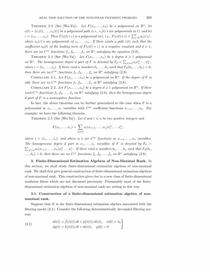
Theorem 2.3 (See [Wu-Ya]). Let F (x1, . . . , xn) be a polynomial on Rn, let
c(t) = (c1(t), . . . , cn(t)) be a polynomial path (i.e., ci(t)’s are polynomials in t), and let
ε = (ε1, . . . , εn). Then F (c(t)+ε) is a polynomial in t, i.e., F (c(t)+ε) =∑d
j=0 aj(ε)tj,
where aj(ε)’s are polynomials of ε1, . . . , εn. If there exists a path c(t) such that the
coefficient ad(t) of the leading term of F (c(t) + ε) is a negative constant and d > 1,
there are no C∞ functions f1, f2, . . . , fn on Rn satisfying the equation (2.8).
Theorem 2.4 (See [Wu-Ya]). Let F (x1, . . . , xn) be a degree d > 1 polynomial
on Rn. The homogeneous degree d part of F is denoted by Fd =
∑|i|=d aix
i11 . . . xin
n ,
where i = (i1, . . . , in). If there exist n numbers b1, . . . , bn such that Fd(b1, . . . , bn) < 0,
then there are no C∞ functions f1, f2, . . . , fn on Rn satisfying (2.8).
Corollary 2.1. Let F (x1, . . . , xn) be a polynomial on Rn. If the degree of F is
odd, there are no C∞ functions f1, f2, . . . , fn in Rn satisfying (2.8).
Corollary 2.2. Let F (x1, . . . , xn) be a degree d > 1 polynomial on Rn. If there
exist C∞-functions f1, f2, . . . , fn on Rn satisfying (2.8), then the homogeneous degree
d part of F is a nonnegative function.
In fact, the above theorems can be further generalized to the case when F is a
polynomial in x1, . . . , xr variables with C∞ coefficient functions xr+1, . . . , xn. For
example, we have the following theorem.
Theorem 2.5 (See [Wu-Ya]). Let d and r 6 n be two positive integers and
F (x1, . . . , xn) =∑
|i|6d
ai(xr+1, . . . , xn)xi11 , . . . xir
r ,
where i = (i1, . . . , ir), and where ai’s are C∞ functions in xr+1, . . . , xn variables.
The homogeneous degree d part in x1, . . . , xr variables of F is denoted by Fd =∑
|i|=d ai(xr+1, . . . , xn)xi11 . . . xir
r . If there exist n numbers b1, . . . , bn such that Fd(b1,
. . . , bn) < 0, then there are no C∞ functions f1, f2, . . . , fn on Rn satisfying (2.8).
3. Finite-Dimensional Estimation Algebras of Non-Maximal Rank. In
this section, we shall study finite-dimensional estimation algebras of non-maximal
rank. We shall first give general construction of finite-dimensional estimation algebras
of non-maximal rank. This construction gives rise to a new class of finite-dimensional
nonlinear filters which are not discussed previously. Presumably most of the finite-
dimensional estimation algebras of non-maximal rank are arising in this way.
3.1. Construction of a finite-dimensional estimation algebra of non-
maximal rank.
Suppose that E is the finite-dimensional estimation algebra associated with the
filtering model (2.1). Consider the following deterministically decoupled filtering sys-
tem:
(3.1)dx(t) = f(x(t)) dt + g(x(t)) dv(t), x(0) = x0
dy(t) = h(x(t)) dt + dw(t), y(0) = 0

310 STEPHEN S. T. YAU
Here x = (x1, . . . , xn, xn+1, . . . , xn+k), f(x(t)) = (f1(x1, . . . , xn), . . . , fn(x1, . . . , xn),
fn+1(xn+1, . . . , xn+k), . . . , fn+k(xn+1, . . . , xn+k)), g(x(t)) = orthogonal matrix,
h(x(t)) = h(x1, . . . , xn), and v and w have components which are independent, stan-
dard Brownian processes.
Let E be the estimation algebra associated with (3.1). We shall show that E is
isomorphic to E as a Lie algebra. Observe that
ωij =∂fj
∂xi
− ∂fi
∂xj
=
∂fj
∂xi
(x) − ∂fi
∂xj
(x) = ωij if 16 i, j6n
0 if i>n, j6n or i6n, j > n,
∂fj
∂xi
(xn+1, . . . , xn+k)
− ∂fi
∂xj
(xn+1, . . . , xn+k), i, j>n,
L0 =1
2
( n+k∑
i=1
Di2−η
),
where
Dn+i =∂
∂xn+i
− fn+i(xn+1, . . . , xn+k), 1 6 i 6 k,
η(x) = η(x) +
n+k∑
i=n+1
∂fj
∂xi
(xn+1, . . . , xn+k) +
n+k∑
i=n+1
fi2(xn+1, . . . , xn+k).
Lemma 3.1. If F is a differential operator in x1, . . . , xn variables of order r,
then [F, η(x1, . . . , xn, xn+1, . . . , xn+k)] = [F, η(x1, . . . , xn)] is a differential operator of
order r − 1 in x1, . . . , xn variables.
Lemma 3.2. Let F be a differential operator of order r in x1, . . . , xn variables.
Then for n + 1 6 j 6 n + k, [Dj2, F ] = 0.
Lemma 3.3. For any differential operator F in x1, . . . , xn variables, [L0, F ] =
[L0, F ].
Theorem 3.1 (Rasoulian–Yau [Ra-Ya]). The estimation algebra E associated
with the filtering model (3.1) is isomorphic to the estimation algebra E associated
with the filtering model (2.1), and E consists of a basis such that all elements in
this basis are differential operators in x1, . . . , xn variables except L0. Furthermore,
Ω =(
∂fj
∂xi− ∂fi
∂xj
)is given by Ω = ( Ω 0
0 A ), where Ω is the n × n matrix(
∂fj
∂xi− ∂fi
∂xj
)
associated with (2.1) and A is a k× k matrix with (i, j)-entry(
∂fn+j
∂xn+i− ∂fn+i
∂xn+j
)(xn+1,
. . . , xn+k).
Remark 3.1. (1) The finite-dimensional estimation algebra E is of non-maximal
rank if k > 0. Observe that A is quite arbitrary. (2) We would like to emphasize that
the orthogonal matrix g(x1, . . . , xn, xn+1, . . . , xn+k) is arbitrary and is not necessarily

REAL TIME SOLUTION OF THE NONLINEAR FILTERING PROBLEM 311
of the form
(g(x1, . . . , xn) 0
0 g(xn+1, . . . , xn+k)
).
So (3.1) is not a direct sum of two filtering systems. This is a central point of Theo-
rem 3.1.
3.2. Classification of finite-dimensional estimation algebras of dimen-
sion less than or equal to four.
Let E =L0, h1, h2, . . . , hm
L.A.
be the estimation algebra associated with the
filtering model (2.1). By Ocone’s theorem, h1, h2, . . . , hm are polynomials at most
degree two. Let h1, h2, . . . , hk, k 6 m be linearly independent and the other hi′s,
k + 1 6 i 6 m be linear combinations of h1, . . . , hk. If k = 1 and h1 = constant, it is
obvious that E is 1-dimensional if and only if h1 = 0, and E is 2-dimensional if and
only if h1 = 1. Thus we have the following proposition.
Proposition 3.1. Let E be the estimation algebra associated with the filtering
model (2.1). Then
(1) dimE = 1 if and only if E = 〈L0〉(2) dimE = 2 if and only if E = 〈L0, 1〉.Theorem 3.2 (Yau–Rasoulian [Ya-Ra]). Let E be the estimation algebra asso-
ciated with the filtering model (2.1). Then dimE 6= 3.
The following theorem gives a structure of 4-dimensional estimation algebras.
Theorem 3.3 ([Ya-Ra]). Suppose that state space of the filtering model (2.1)
is of a dimension greater than one. Then the observation function h(x) is linear
and the linear span of ∇h1, . . . ,∇hm is 1-dimensional. Assume h1(x) = x1. Then
the 4-dimensional estimation algebra has a basis given by 1, x1, D1 = ∂∂x1
− f1 and
L0 = 12
(∑ni=1 D2
i − η). Moreover, ω12 = ω13 = · · · = ω1n = 0, [L0, x1] = D1,
[D1, x1] = 1, [L0, D1] = 12
∂η∂x1
= αx1 + β. where α, β are constants. Also, η =
αx12 + 2βx1 + g(x2, . . . , xn), where g(x2, . . . , xn) is in C∞(Rn−1). In particular,
f1, . . . , fn have to satisfy the equation
(3.2)
n∑
i=1
∂fi
∂xi
+
n∑
i=1
fi2 = (α − 1)x2
1 + 2βx1 + g(x2, . . . , xn)
where α > 1.
3.3. Structure theorem for five-dimensional estimation algebras.
The following lemmas plays an important role in understanding estimation algebra
of non-maximal rank.
Lemma 3.4 (Chiou–Chiueh–Yau [C-C-Y]). For any 1 6 l 6 n, if γi, i = 1, . . . , l,
are polynomials in x1, . . . , xl with coefficients in C∞ functions of xl+1, . . . , xn satis-

312 STEPHEN S. T. YAU
fying
(3.3)∂γj
∂xi
+∂γi
∂xj
= 0 for all 1 6 i, j 6 l,
then each γi is necessarily of the form
(3.4) γi =∑
16j6l
cji (xl+1, . . . , xn)xj + di(xl+1, . . . , xn)
where cji (xl+1, . . . , xn) and di(xl+1, . . . , xn) are C∞ functions and c
ji = −ci
j.
Lemma 3.5. If dimE = 5, then E cannot contain two linear independent degree
one polynomials.
Theorem 3.4 (Chiou–Chiueh–Yau [C-C-Y]). If dimE = 5, then E cannot
contain any degree two polynomial.
Theorem 3.4, above, together with Theorem 3.3 asserts the following Mitter con-
jecture is true for estimation algebras with dimension at most five.
Mitter Conjecture 1. Let E be a finite-dimensional estimation algebra. Then
any function in E is a polynomial of degree at most one.
Now we are ready to state the structure theorem of five-dimensional estimation
algebras.
Theorem 3.5 (Chiou–Chiueh–Yau [C-C-Y]). Suppose that the state space of the
filtering model (2.1) is of dimension at least two. Then the five-dimensional estimation
algebra is isomorphic to to Lie algebra generated by L0 and an observation function
h = x1 with a basis given by 1, x1, D1 = ∂∂x1
− f1(x1, . . . , xn), Y1 = [L0, D1] =∑n
i=1 ωi1Di + 12
∂η∂x1
, L0 = 12
(∑ni=1 Di
2 − η). Moreover, the following holds:
(1) ω1i 6= 0 for some i = 2, . . . , n and each ω1i is of the form
(3.5) ω1i =
n∑
k=2
eikxk + ei for 2 6 i 6 n,
(3.6) eij = −eji, 2 6 i, j 6 n,
where eij and ei are constants.
(2) η is of the form
(3.7) η =( n∑
j=2
ω2ij + c3
)x1
2 + β(x2, . . . , xn)x1 + γ(x2, . . . , xn),
where c3 > 1 is a constant and β(x2, . . . , xn) and γ(x2, . . . , xn) are C∞ func-
tions
(3) There exists a constant c1 such that
(3.8)n∑
j=1
ω1jωji +1
2
∂2y
∂xi∂x1= c1ω1i, 2 6 i 6 n

REAL TIME SOLUTION OF THE NONLINEAR FILTERING PROBLEM 313
(4) There exists constants c0 and c2 such that
(3.9) −1
2
n∑
i,j=1
∂ω1j
∂xi
ωji +1
2
n∑
j=1
ω1j
∂η
∂xj
= c0x1 +c1
2
∂η
∂x1+ c2.
In particular, f1, . . . , fn have to satisfy the following equation:
(3.10)
n∑
i=1
∂fi
∂xi
+
n∑
i=1
fi2 =
( n∑
j=2
ω21j + c3 − 1
)x1
2
+ β(x2, . . . , xn)x1 + γ(x2, . . . , xn).
Moreover, the five-dimensional estimation algebra has the following multiplication ta-
ble.
E 1 x1 D1 Y1 L0
1 0 0 0 0 0
x1 0 0 −1 0 −D1
D1 0 1 0 c3 −Y1
Y1 0 0 −c3 0 −c0x1−c1Y1−c2−c3D1
L0 0 D1 Y1 c0x1+c1Y1+c2+c3D1 0
Corollary 3.1. Suppose that the state space of the filtering model (2.1) is of
dimension at least two. If ω1j, 2 6 j 6 n, are constants, then the five-dimensional
estimation algebra is isomorphic to a Lie algebra generated by L0 and x1 with a basis
given by 1, x1, D1 = ∂∂x1
− f1(x1, . . . xn), Y1 = [L0, D1] =∑n
i=1 ωi1Di + 12
∂η∂x1
,
L0 = 12
(∑ni=1 D2
i − η). Moreover, the following holds:
(1) η is of the form
(3.11) η = ax12 + β(x2, . . . , xn)x1 + γ(x2, . . . , xn)
for some constant a > 1 and C∞ functions β(x2, . . . , xn) and γ(x2, . . . , xn).
(2) There exists constant d1 such that
(3.12)1
2
∂β
∂xi
(x2, . . . , xn) = d1ω1i +
n∑
j=1
ω1jωij for 2 6 i 6 n.
(3) There exist constants d2 and d3 such that
(3.13)n∑
j=1
ω1j
∂β
∂xj
(x2, . . . , xn) = d2
(3.14)n∑
j=1
ω1j
∂γ
∂xj
(x2, . . . , xn) = d1β(x2, . . . , xn) + d3.

314 STEPHEN S. T. YAU
We shall give an example of five-dimensional estimation algebras by using Theo-
rem 3.5. Example 3.1 below is a new class of finite-dimensional estimation algebras.
Example 3.1. Consider the filtering model
dx(t) = f(x(t)) dt + g(x(t)) dv(t)
dy(t) = h(x(t)) dt + dw(t)
where f1 = ax1, f2 = bx1x3, f3 = −bx1x2, fi = gi(x4, . . . , xn), 4 6 i 6 n, h(x) = x1,
and a, b are nonzero constants. Then
ω12 =∂f2
∂x1− ∂f1
∂x2= bx3, ω13 =
∂f3
∂x1− ∂f1
∂x3= −bx2
ω23 =∂f3
∂x2− ∂f2
∂x3= −2bx1, ω1j =
∂fj
∂x1− ∂f1
∂xj
= 0, 4 6 i 6 n.
n∑
i=1
fi2 +
n∑
i=1
∂fi
∂xi
= a2x12 + b2x1
2x32 + b2x1
2x22
+n∑
i=4
gi2(x4, . . . , xn) + a +
n∑
i=4
∂gi
∂xi
(x4, . . . , xn)
=( n∑
i=1
ω1i2 + a2
)x1
2 +
n∑
i=4
gi2(x4, . . . , xn) + a
+n∑
i=4
∂gi
∂xi
(x4, . . . , xn).
It is easy to check that ω1i, 1 6 i 6 n, satisfy (3.5), η is of the form (3.7) with
c3 = a2 + 1 satisfying (3.8) and (3.9) with c0 = 2b2, c1 = c2 = 0. The estimation
algebra E is five-dimensional with basis 1, x1, D1, Y1 = bx3D2 − bx2D3 + (a2 + 1 +
b2x22 + b2x3
2)x1, L0.
3.4. Classification of estimation algebras with state dimension 2.
In this subsection, we shall fix the state dimension 2 and consider all finite-
dimensional estimation algebras.
Theorem 3.6 (Wu–Yau [Wu-Ya]). Suppose that the state dimension of the fil-
terings model (2.1) is two. Assume dim E < ∞ and Y = p(x)D2 + function is an
element in E. Then p is a polynomial in x1, x2, of degree at most one.
Theorem 3.7 (Wu–Yau [Wu-Ya]). Suppose that the state space dimension of
the filtering model (2.1) is two. If dimE < ∞ and φ ∈ E, then φ is a polynomial of
degree at most one.
Theorem 3.8 (Wu–Yau [Wu-Ya]). Suppose that the state dimension of the fil-
tering model (2.1) is two. If E has linear rank 1 and is finite-dimensional, then the
Wong matrix Ω has constant entries

REAL TIME SOLUTION OF THE NONLINEAR FILTERING PROBLEM 315
We are now read to classify all finite-dimensional estimation algebras with state
dimension 2. First assume E has linear rank 1. By Theorem 3.7, hi’s must be degree
at most 1 polynomial in x1. By Theorem 3.8, ω12 is a constant.
(i) ω12 = 0, [L0, D1] = 12
∂η∂x1
∈ E. Thus, η must be a degree 2 polynomial in x1
plus a C∞-function in x2. E = Lo, x1, D1, 1. For example, f1 = x1, f2 = sin x2,
h1 = x1, η = 2x12 + 1 + cosx2 + sin2 x2.
(ii) If ω12 6= 0, let
(3.15) A1 := [L0, D1] = ω12D2 +1
2
∂η
∂x1∈ E
(3.16) A2 := [D1, A1] = −ω212 +
1
2
∂2η
∂x12∈ E
A3 := [L0, A1] =
(1
2
∂2η
∂x12− ω2
12
)D1 +
1
2
∂2η
∂x1∂x2D2
+1
2ω12
∂η
∂x2+
1
4
∂3η
∂x13
+1
4
∂3η
∂x1∂x22∈ E(3.17)
By (3.16), η = d0x13 + d1x1
2 + e2(x2)x1 + e3(x2). By Theorem 2.5, d0 = 0. By (3.17)
and D1 ∈ E.
(3.18)1
2
∂2η
∂x1∂x2D2 +
1
2ω12
∂η
∂x2+
1
4
∂3η
∂x1∂x22∈ E.
By Theorem (3.6), ∂2η∂x1∂x2
= e′2(x2) is a polynomial of degree at most 1. Thus e2 is a
polynomial of degree at most 2 in x2. By substituting e2 and e3 into η and removing
D1, x1, and 1 from (3.15) and (3.18), one has
A1 = ω12D2 +1
2e2 ∈ E(3.19)
A3 =1
2e′2D2 +
1
2ω12(e
′2x1 + e′3) ∈ E(3.20)
If e2 is a degree 2 polynomial in x2, then [A1, A3] − 12e′′2A1 = 1
2ω212e
′′3 − 1
4 (e2e′′2 +
e′2e′2) + 1
2ω212e
′′2x1 ∈ E. Since the degree 2 term of e2e
′′2 + e′2e
′2 will never be zero,
e3(x2) must be a degree 4 polynomial. Now, consider
B1 = [L0, A3]
=1
2e′′1D2
2 +1
2ω12(e
′′2x1 + e′′3)D2 +
1
4e′2(e
′2x1 + e′3) +
1
4ω12e
′′3 ∈ E
B2 = [L0, B1] =1
2e′′2[L0, D2
2]+ [L0,
1
2ω12(e
′′2x1 + e′′3)D2]
=1
2ω12e
′′3D2
2 − 1
2ω12e
′′2D2D1 + function ∈ E.
From the discussion of the proof of Lemma 4.13 (iii) in [Wu-Ya], e′′′3 must be a con-
stant, Contradiction! Hence e2 must be a degree 1 polynomial.

316 STEPHEN S. T. YAU
Consider ω12A3 − 12e′1A1 = 1
2ω212e
′2x1 + 1
2ω212e
′3 − 1
4e′2e2 ∈ E ⇒ 12ω2
12e′3 − 1
4e′2e2
is independent of x2 and e3 must be a degree 2 polynomial. Hence, η is a degree 2
polynomial in x1 and x2. E is of dimension 5 and E = L0, x1, D1, D2 + cx2, 1.For example, f1 = 5x1 − 3x2, f2 = 4x2, h1 = x1. Then ω12 = 3 and η =
26x12 − 30x1x2 + 25x2
2 + 9. It is easy to show that E = L0, x1, D1, D2 − 5x2, 1.If E has linear rank 0, hi’s must be constants, and E = L0 or E = L0, 1.If E has linear rank 2, E is of maximal rank. The Ω-matrix must have constant
entries and E = L0, x1, x2, D1, D2, 1 by the theorem of Yau and Hu [Ya-Hu3]. In
summary, we have the following.
Theorem 3.9 (Wu–Yau [Wu-Ya]). Let n = 2. If E is finite-dimensional, then
(1) if hi’s are constants, E = L0 or E = L0, 1;(2) otherwise, Ω-matrix has constant entries. hi’s must be affine in x1 and x2.
E has dimension of either 4, 5, or 6.
Moreover, from the above discussion, it is easy to see that if E is finite-dimension-
al, it has only elements with order less than or equal to 2. Thus, the Levine conjecture
holds for the finite-dimensional estimation algebras with state dimension 2.
4. Direct Method of Solving the DMZ Equation. The direct method was
first introduced by Yau–Yau [Ya-Ya1][Ya-Ya2] to solve DMZ equations arising from a
linear filtering model or an exact filtering model. This direct method was generalized
by Yau–Hu [Ya-Hu1] [Ya-Hu2] to treat a more general filtering system.
Recall that in 1990, Yau [Ya1] (cf. [Ya2] for detailed version) first studied the
filtering model (2.1) with the following conditions:
(c′1)∂fj
∂xi
− ∂fi
∂xj
= constant cij for all 1 6 i, j 6 n.
This was called the Yau filtering model in [Ch]. The Yau filtering model includes
linear filtering model and exact filtering model. By Theorem 3.3, we know that (c′1)
is equivalent to the following condition:
(4.1) (c1) fi(x) = li(x) +∂F
∂xi
(x), 1 6 i 6 n
where li(x) =∑n
j=1 dijxj + di for 1 6 i 6 n and F is a C∞ function.
A theorem in [Ya2] tells us that h1, . . . , hm are polynomials of degree at most one
if the Yau filtering model has a finite-dimensional estimation algebra. So we list the
following condition:
(4.2) (c2) hi(x) =
n∑
j=1
cijxj + ci, 1 6 i 6 m
where cij and ci are constants.

REAL TIME SOLUTION OF THE NONLINEAR FILTERING PROBLEM 317
Moreover, by a theorem in [Ya2], we know that η(x) is a polynomial of degree at
most two for Yau filtering models with finite-dimensional estimation algebra. Hence
we assume the following condition:
(4.3) (c3) η(x) =
n∑
i,j=1
ηijxixj +
n∑
i=1
ηixi + η0
where ηij , ηi, and η0 are constants.
Lemma 4.1 (Yau–Hu [Ya-Hu2]). Equation (2.4) is equivalent to the following
equation
(4.4)
∂u
∂t(t, x) =
1
2∆u(t, x) +
n∑
i=1
θi(t, x)∂u
∂x2(t, x) + θ(t, x)u(t, x)
u(0, x) = σ0(x)
where
θi(t, x) =
m∑
j=1
yj(t)∂hj
∂xi
(x) − fi(x),
θ(t, x) =1
2
( n∑
i=1
θi2(t, x) +
n∑
i=1
∂θi
∂xi
(t, x) − η(x)).
Theorem 4.1 (Yau–Hu [Ya-Hu2]). Suppose u(t, x) is a solution of (4.4) and
(4.5) u(t, x) = eΛ(t,x)u(t, x + b(t))
Then u(t, x) is the solution of the following Kolmogorov equation:
(4.6)
∂u
∂t(t, x) =
1
2∆u(t, x) −
n∑
i=1
Hi(x)∂u
∂xi
(t, x) − P (x)u(t, x)
u(0, x) = eΛ(0,x)u(0, x + b(0)).
if we can choose Hi(x) and P (x) such that Λ(t, x) satisfy the following systems:
(4.7) b′i(t) −∂Λ
∂xi
(t, x) + H(x) + θi(t, x + b(t)) ≡ 0 1 6 i 6 n
(4.8)∂Λ
∂t(t, x) − 1
2
n∑
i=1
(b′i(t))2 −
n∑
i=1
θi(t, x + b(t))b′n(t) − 1
2η(x + b(t))
+1
2
n∑
i=1
Hi2(x) − 1
2
n∑
i=1
∂Hi
∂xi
(x) + P (x) ≡ 0
Moreover, if u,∂u
∂x1, . . . ,
∂u
∂xn
are linearly independent, then (4.7) and (4.8) are also
necessary conditions for (4.6).

318 STEPHEN S. T. YAU
Next if we assume that condition (c3) holds, then
(4.9) η(x + b(t)) = η(x) +
n∑
i=1
Bi(t)xi + B(t)
where
Bi(t) =
n∑
j=1
(nij + ηji)bj(t),
B(t) =
n∑
i,j=1
nijbi(t)bj(t) +
n∑
i=1
ηibi(t)
The following theorem says that in many situations if the solution of (4.4) can be
represented in the form of (4.5) and (4.6), then condition (c1) in (4.1) holds.
Theorem 4.2 (Yau–Hu [Ya-Hu2]). Assume conditions (c2) and (c3) hold. Sup-
pose u(t, x) is a solution of (4.4) and
u(t, x) = eΛ(t,x)u(t, x + b(t))
where b′i(t), 1 6 i 6 n, are linearly independent and u(t, x) is the solution of the
following Kolmogorov equation:
∂u
∂t(t, x) =
1
2∆u(t, x) −
n∑
i=1
Hi(x)∂u
∂xi
(t, x) − P (x)u(t, x)
u(0, x) = eΛ(0,x)u(0, x + b(0)).
Furthermore, let
Λ(t, x) = c(t) + G(x) +
n∑
i=1
aj(t)xj − F (x + b(t)).
If we can choose H(x), G(x), and P (x) such that
(4.10)1
2
n∑
i=1
Hi2(x) − 1
2
n∑
i=1
∂H
∂xi
(x) − 1
2η(x) + P (x) ≡ 0,
then
fi(x) =∂F
∂xi
(x) + li(x), 1 6 i 6 n,
where li(x) =∑n
j=1 dijxj + di, dij and di are constants, i.e., condition (c1) holds.
The following theorem plays an important role in our direct method.
Theorem 4.3 (Yau-Hu [Ya-Hu2]). Consider the filtering model (2.1) with con-
ditions (c1), (c2), and (c3). Then the solution u(t, x) for the DMZ equation (2.4) or
(4.4) is reduced to the solution of u(t, x) for the Kolmogorov equation
∂u
∂t(t, x) =
1
2∆u(t, x) −
n∑
i=1
Hi(x)∂u
∂xi
(t, x) − P (x)u(t, x)
u(0, x) = eG(x)−F (x)σ0(x)
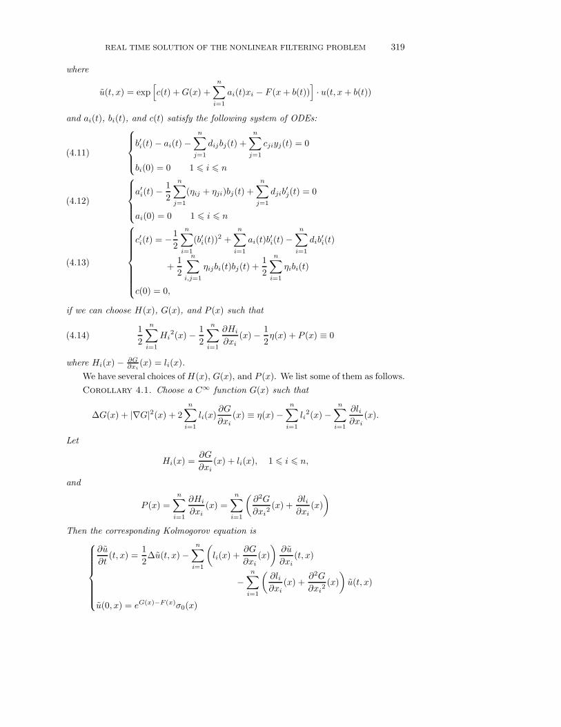
REAL TIME SOLUTION OF THE NONLINEAR FILTERING PROBLEM 319
where
u(t, x) = exp[c(t) + G(x) +
n∑
i=1
ai(t)xi − F (x + b(t))]· u(t, x + b(t))
and ai(t), bi(t), and c(t) satisfy the following system of ODEs:
b′i(t) − ai(t) −n∑
j=1
dijbj(t) +
n∑
j=1
cjiyj(t) = 0
bi(0) = 0 1 6 i 6 n
(4.11)
a′i(t) −
1
2
n∑
j=1
(ηij + ηji)bj(t) +
n∑
j=1
djib′j(t) = 0
ai(0) = 0 1 6 i 6 n
(4.12)
c′i(t) = −1
2
n∑
i=1
(b′i(t))2 +
n∑
i=1
ai(t)b′i(t) −
n∑
i=1
dib′i(t)
+1
2
n∑
i,j=1
ηijbi(t)bj(t) +1
2
n∑
i=1
ηibi(t)
c(0) = 0,
(4.13)
if we can choose H(x), G(x), and P (x) such that
(4.14)1
2
n∑
i=1
Hi2(x) − 1
2
n∑
i=1
∂Hi
∂xi
(x) − 1
2η(x) + P (x) ≡ 0
where Hi(x) − ∂G∂xi
(x) = li(x).
We have several choices of H(x), G(x), and P (x). We list some of them as follows.
Corollary 4.1. Choose a C∞ function G(x) such that
∆G(x) + |∇G|2(x) + 2n∑
i=1
li(x)∂G
∂xi
(x) ≡ η(x) −n∑
i=1
li2(x) −
n∑
i=1
∂li
∂xi
(x).
Let
Hi(x) =∂G
∂xi
(x) + li(x), 1 6 i 6 n,
and
P (x) =
n∑
i=1
∂Hi
∂xi
(x) =
n∑
i=1
(∂2G
∂xi2(x) +
∂li
∂xi
(x)
)
Then the corresponding Kolmogorov equation is
∂u
∂t(t, x) =
1
2∆u(t, x) −
n∑
i=1
(li(x) +
∂G
∂xi
(x)
)∂u
∂xi
(t, x)
−n∑
i=1
(∂li
∂xi
(x) +∂2G
∂xi2(x)
)u(t, x)
u(0, x) = eG(x)−F (x)σ0(x)

320 STEPHEN S. T. YAU
where
u(t, x) = exp[c(t) + G(x) +
n∑
i=1
ai(t)xi − F (x + b(t))]· u(t, x + b(t))
and ai(t), bi(t), and c(t) satisfy ODEs (4.11), (4.12) and (4.13).
Corollary 4.2. Choose
G(x) ≡ 0
P (x) =1
2η(x) − 1
2
n∑
i=1
li2(x) − 1
2
n∑
i=1
∂li
∂xi
(x)
Hi(x) = li(x), 1 6 i 6 n.
Then the corresponding Kolmogorov equation becomes
∂u
∂t(t, x) =
1
2∆u(t, x) −
n∑
i=1
li(x) +∂u
∂xi
(t, x)
− 1
2
( n∑
i=1
li2(x) −
n∑
i=1
∂li
∂xi
(x) − η(x))u(t, x)
u(0, x) = e−F (x)σ0(x)
where
u(t, x) = exp
[c(t) +
n∑
i=1
ai(t)xi − F (x + b(t))
]· u(t, x + b(t))
and ai(t), bi(t), and c(t) satisfy ODEs (4.11), (4.12) and (4.13).
Corollary 4.3. Choose a C∞ function G(x) such that ∂G∂xi
(x) = −li(x) if
dij = dji for 1 6 i, j 6 n. Let P (x) = 12η(x) and Hi(x) ≡ 0, 1 6 i 6 n. Then the
corresponding Kolmogorov equation becomes
∂u
∂t(t, x) =
1
2∆u(t, x) − 1
2η(x)u(t, x)
u(0, x) = eG(x)−F (x)σ0(x).
where
u(t, x) = exp[c(t) + G(x) +
n∑
i=1
ai(t)xi − F (x + b(t))]· u(t, x + b(t))
and ai(t), bi(t), and c(t) satisfy ODEs (4.11), (4.12) and (4.13).
Corollary 4.4. Choose
G(x) = F (x)
P (x) =1
2η(x) − 1
2
n∑
i=1
fi2(x) +
1
2
n∑
i=1
∂fi
∂xi
(x)
Hi(x) = fi(x), 1 6 i 6 n.

REAL TIME SOLUTION OF THE NONLINEAR FILTERING PROBLEM 321
Then the corresponding Kolmogorov equation becomes
∂u
∂t(t, x) =
1
2∆u(t, x) −
n∑
i=1
fi(x) +∂u
∂xi
(t, x)
+1
2
( n∑
i=1
fi2(x) −
n∑
i=1
∂fi
∂xi
(x) − η(x))u(t, x)
u(0, x) = σ0(x)
where
u(t, x) = exp[c(t) +
n∑
i=1
ai(t)xi + F (x) − F (x + b(t))]· u(t, x + b(t))
and ai(t), bi(t), and c(t) satisfy ODEs (4.11), (4.12) and (4.13).
5. New Algorithms in Real Time Solution of the Nonlinear Filtering
Problem. The purpose of this section is to describe our new algorithms which can
solve all engineering problems in real time. In section 5.1, we give some detail why
the solution arising from our algorithm converges to the true solution of the DMZ
equation for the filtering model (2.1). In section 5.2, we describe how our algorithm
works for the general filtering model (1.1).
5.1. Yau–Yau algorithm of solving nonlinear filtering problems.
The direct method described in the previous section works very nicely for the Yau
filtering system and it is very easy to implement. However, in all the direct methods
in [Ya-Ya1] [Ya-Ya2] [Ya-Hu1][Ya-Hu2], they need to assume that all the observation
terms hi(x), 1 6 i 6 m, are degree one polynomials. On the other hand, in many
practical examples, e.g., tracking problem, the observation terms may be nonlinear. In
2000, we [Ya-Ya3] proposed a novel algorithm to solve the DMZ equation in real time
and memoryless way. Under the assumptions that the drift terms fi(x), 1 6 i 6 n,
and their first and second derivatives, and the observation terms hi(x), 1 6 i 6 m,
and their first derivatives, have linear growth, we showed that the solution obtained
from our algorithms converges to the true solution of the DMZ equation. Recently we
[Ya-Ya4] show that under very mild conditions which essentially say that the growth
of |h| is greater than the growth of |f |, the DMZ equation admits a unique nonnegative
solution u which can be approximated by solutions uR of DMZ equation on the ball
BR with uR|∂BR= 0. The rate of convergence can be efficiently estimated in L1-norm.
The solutions uR can in turn be approximated efficiently by an algorithm depending
only on solving the time independent Kolmogorov equation on BR. Our algorithm
can solve practically all engineering problems including the cubic sensor problem in
real time and memoryless manner.
It is shown in [Ya-Ya3] that the robust DMZ equation can be written in the
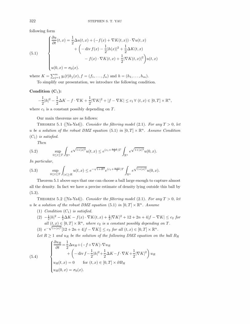
322 STEPHEN S. T. YAU
following form
(5.1)
∂u
∂t(t, x) =
1
2∆u(t, x) + (−f(x) + ∇K(t, x)) · ∇u(t, x)
+
(− div f(x) − 1
2|h(x)|2 +
1
2∆K(t, x)
− f(x) · ∇K(t, x) +1
2|∇K(t, x)|2
)u(t, x)
u(0, x) = σ0(x).
where K =∑m
j=1 yi(t)hj(x), f = (f1, . . . , fn) and h = (h1, . . . , hm).
To simplify our presentation, we introduce the following condition.
Condition (C1):
−1
2|h|2 − 1
2∆K − f · ∇K +
1
2|∇K|2 + |f −∇K| ≤ c1 ∀ (t, x) ∈ [0, T ]× R
n,
where c1 is a constant possibly depending on T .
Our main theorems are as follows:
Theorem 5.1 ([Ya-Ya4]). Consider the filtering model (2.1). For any T > 0, let
u be a solution of the robust DMZ equation (5.1) in [0, T ] × Rn. Assume Condition
(C1) is satisfied.
Then
(5.2) sup0≤t≤T
∫
Rn
e√
1+|x|2u(t, x) ≤ e(c1+n+12
)T
∫
Rn
e√
1+|x|2u(0, x).
In particular,
(5.3) sup0≤t≤T
∫
|x|≥R
u(t, x) ≤ e−√
1+R2
e(c1+n+1
2)T
∫
Rn
e√
1+|x|2u(0, x).
Theorem 5.1 above says that one can choose a ball large enough to capture almost
all the density. In fact we have a precise estimate of density lying outside this ball by
(5.3).
Theorem 5.2 ([Ya-Ya4]). Consider the filtering model (2.1). For any T > 0, let
u be a solution of the robust DMZ equation (5.1) in [0, T ]× Rn. Assume
(1) Condition (C1) is satisfied.
(2) − 12 |h|2 − 1
2∆K − f(x) · ∇K(t, x) + 12 |∇K|2 + 12 + 2n + 4|f −∇K| ≤ c2 for
all (t, x) ∈ [0, T ]× Rn, where c2 is a constant possibly depending on T .
(3) e−√
1+|x|2[12 + 2n + 4|f −∇K|] ≤ c3 for all (t, x) ∈ [0, T ]× Rn.
Let R ≥ 1 and uR be the solution of the following DMZ equation on the ball BR
(5.4)
∂uR
∂t=
1
2∆uR+(−f +∇K)·∇uR
+
(− div f− 1
2|h|2+
1
2∆K−f · ∇K+
1
2|∇K|2
)uR
uR(t, x) = 0 for (t, x) ∈ [0, T ]× ∂BR
uR(0, x) = σ0(x).

REAL TIME SOLUTION OF THE NONLINEAR FILTERING PROBLEM 323
Let v = u − uR. Then v ≥ 0 for all (t, x) ∈ [0, T ]× BR and
(5.5)
∫
BR
φv(T, x) ≤ ec2T − 1
c2c3e
−Re(c1+n+1
2)T
∫
Rn
e√
1+|x|2u(0, x)
where φ(x) = e|x|4
R3 − 2|x|2
R − e−R. In particular
(5.6)
∫
B R2
v(T, x)
≤ 2(ec2T − 1)
c2c3e
− 916
Re(c1+n+1
2)T
∫
Rn
e√
1+|x|2u(0, x).
Theorem 5.2 above says that we can approximate u by uR. The approximation
is good if R is large enough. In fact we have a precise error estimate of this approxi-
mation by (5.6).
Theorem 5.3 ([Ya-Ya4]). Let Ω be a bounded domain in Rn. Let F : [0, T ]×Ω →
Rn be a family of vector fields C∞ in x and Holder continuous in t with exponent α
and J : [0, T ]×Ω → R be a C∞ function in x and Holder continuous in t with exponent
α such that the following properties are satisfied
(5.7) | divF (t, x)| + 2|J(t, x)| + |F (t, x)| ≤ c for (t, x) ∈ [0, T ]× Ω
(5.8) |F (t, x) − F (t, x)| + | div F (t, x) − div F (t, x)|+ |J(t, x) − J(t, x)| ≤ c1|t − t|α
for (t, x), (t, x) ∈ [0, T ]× Ω.
Let u(t, x) be the solution on [0, T ]× Ω of the equation
(5.9)
∂u
∂t(t, x) =
1
2∆u(t, x) + F (t, x) · ∇u(t, x) + J(t, x)u(t, x)
u(0, x) = σ0(x)
u(t, x)∣∣∂Ω
= 0.
For any 0 ≤ τ ≤ T , let Pk = 0 = τ0 < τ1 < τ2 < · · · < τk = τ be a partition of [0, τ ]
where τi = iτk. Let ui(t, x) be the solution on [τi−1, τi] × Ω of the following equation
(5.10)
∂ui
∂t(t, x) =
1
2∆ui(t, x) + F (τi−1, x) · ∇ui(t, x)
+ J(τi−1, x)ui(t, x)
ui(τi−1, x) = ui−1(τi−1, x)
ui(t, x)∣∣∂Ω
= 0.

324 STEPHEN S. T. YAU
Here we use the convention u0(t, x) = σ(x). Then the solution u(t, x) of (5.9) can
be computed by means of the solution ui(t, x) of (5.10). More specifically, u(τ, x) =
limk→∞
uk(τk, x) in L1-sense on Ω and the following estimate holds
(5.11)
∫
Ω
|u − uk|(τk, x) ≤ 2c2
α + 1
T α+1ecT
kα
where
(5.12) c2 =c1ecT+c1
√Vol (Ω)ec2T
√2c2T
∫
Ω
u2(0, x)+
∫
Ω
|∇u(0, x)|2.
The right hand side of (5.11) goes to zero as k → ∞.
In case (5.9) and (5.10) are DMZ equations, i.e., F (t, x) = −f(x) + ∇K and
J(t, x) = − div f − 12 |h|2 + 1
2∆K − f · ∇K + 12 |∇K|2, where K =
∑mj=1 yj(t)hj(x),
by Proposition 5.1 below (which is similar to Proposition 3.1 of [Ya-Ya3]), ui(τi, x)
can be computed by ui(τi, x) where ui(t, x) for τi−1 ≤ t ≤ τi satisfies the following
Kolmogorov equation
(5.13)
∂ui
∂t(t, x)=
1
2∆ui(t, x)−
n∑
j=1
fj(x)∂ui
∂xj
(t, x)
−(divf(x)+
1
2
m∑
j=1
h2j(x)
)ui(t, x)
ui(τi−1, x)= exp( m∑
j=1
(yj(τi−1)−yj(τi−2))hj(x))ui−1(τi−1, x).
In fact
(5.14) ui(τi, x) = exp(−
m∑
j=1
yj(τi−1)hj(x))ui(τi, x).
Therefore theoretically to solve the DMZ equation in a real time manner, we only
need to compute the following Kolmogorov equations off-line
∂u
∂t(t, x) =
1
2∆u(t, x) −
n∑
j=1
fj(x)∂u
∂xj
(t, x)
−(
div f(x) +1
2
m∑
j=1
h2j(x)
)u(t, x)
u(0, x) = φi(x)
where φi(x) is an orthonormal base in L2(Rn). The only real time computation
here is to express arbitrary initial condition φ(x) as the linear combination of φi(x).
But this can be done by means of parallel computation.
The following Proposition 5.1 plays a fundamental role in our real time solution
to the robust DMZ equation (5.1) in memoryless manner.

REAL TIME SOLUTION OF THE NONLINEAR FILTERING PROBLEM 325
Proposition 5.1. u(t, x) satisfies the following Kolmogorov equation
∂u
∂t(t, x) =
1
2∆u(t, x) − f(x) · ∇u(t, x)
−(
div f(x) +1
2
m∑
i=1
h2i (x)
)u(t, x)(5.15)
for τℓ−1 ≤ t ≤ τℓ if and only if
(5.16) u(t, x) = e−
m∑i=1
yi(τℓ−1)hi(x)u(t, x)
satisfies the robust DMZ equation with observation being frozen at y(τℓ−1)
∂u
∂t(t, x) =
1
2∆u(t, x) + (−f(x) + ∇K(τℓ−1, x)) · ∇u(t, x)
+
(− div f(x) − 1
2|h(x)|2 +
1
2∆K(τℓ−1, x)(5.17)
−f(x) · ∇K(τℓ−1, x) +1
2|∇K(τℓ−1, x)|2
)u(t, x).
We remark that (5.17) is obtained from the robust DMZ equation by freezing the
observation term y(t) to y(τℓ−1). We shall show that the solution of (5.17) approxi-
mates the solution of the robust DMZ equation very well in L1-sense.
Suppose that u(t, x) is the solution of the robust DMZ equation and we want to
compute u(τ, x). Let Pk = 0 = τ0 < τ1 < τ2 < . . . < τk = τ be a partition of [0, τ ]
where τi = iτk
. Let ui(t, x) be a solution of the following partial differential equation
for τi−1 ≤ τ ≤ τi:
(5.18)
∂ui
∂t(t, x) =
1
2∆ui(t, x) + (−f(x) + ∇K(τi−1, x)) · ∇ui(t, x)
+
(− div f(x) − 1
2|h(x)|2
+1
2∆K(τi−1, x)
− f(x) · ∇K(τi−1, x)
+1
2|∇K(τi−1, x)|2
)ui(t, x)
ui(τi−1, x) = ui−1(τi−1, x).
By Theorem 5.3 we have that u(τ, x) = limk→∞
uk(τk, x) in L1-sense. By Proposition
5.1, u1(τ1, x) can be computed by u1(τ1, x) where u1(t, x) for 0 ≤ t ≤ τ1 satisfies
equation (5.15) with initial condition
(5.19) u1(0, x) = σ0(x).
In fact
(5.20) u1(τ1, x) = u1(τ1, x).

326 STEPHEN S. T. YAU
In general Proposition 5.1 tells us that for i ≥ 2, ui(τi, x) can be computed by ui(τi, x),
where ui(t, x) for τi−1 ≤ t ≤ τi satisfies equation (5.15) with initial condition
(5.21) ui(τi−1, x) = exp[ m∑
j=1
(yj(τi−1) − yj(τi−2))hj(x)]ui−1(τi−1, x)
where the last initial condition comes from
ui(τi−1, x)
= ui(τi−1, x) exp( m∑
j=1
yj(τi−1)hj(x))
= ui−1(τi−1, x) exp( m∑
j=1
yj(τi−1)hj(x))
= exp(−
m∑
j=1
yj(τi−2)hj(x))ui−1(τi−1, x) exp
( m∑
j=1
yj(τi−1)hj(x))
= exp[ m∑
j=1
(yj(τi−1) − yj(τi−2)hj(x)]ui−1(τi−1, x).
In fact,
(5.22) ui(τi, x) = exp(−
m∑
j=1
yj(τi−1)hj(x))ui(τi, x)
Theorem 5.4 ([Ya-Ya4]). Let uR be the solution of (5.4) the DMZ equation
on BR. Assume that
(1) f(x) and h(x) have at most polynomial growth.
(2) For any 0 ≤ t ≤ T , there exist positive integer m and positive constants c′
and c′′ independent of R such that the following two inequalities hold on Rn.
(a) m2
2 |x|2m−2− m2 (m+n−2)|x|m−2−m|x|m−2x · (f −∇K)− ∆K
2 − 12 |h|2−
f · ∇K + 12 |∇K|2 ≥ −c′
(b)∣∣m2|x|2m−2
2 − m(m+n−2)2 |x|m−2 − m|x|m−2(f −∇K) · x
∣∣≤ m(m+1)
2 |x|2m−2 + c′′
(3) − 12 |h|2 − 1
2∆K −n∑
j=1
fj∂K∂xj
+ 12 |∇K|2 ≤ c1 for all (t, x) ∈ [0, T ] × R
n where
c1 is a constant possibly depending on T .
Then for any R0 < R,∫
BR0
(e−|x|m − e−Rm
0
)uR(T, x)
≥ e−c′T
∫
BR0
(e−|x|m − e−Rm0 )σ0(x)
+e−Rm
0
c′
(m(m + 1)
2R2m−2
0 + c′′)(
1 − ec′T)∫
BR
σ0(x).

REAL TIME SOLUTION OF THE NONLINEAR FILTERING PROBLEM 327
In particular, the solution u of the robust DMZ equation on Rn has the following
estimate
∫
Rn
e−|x|mu(T, x) ≥ e−c′T
∫
Rn
e−|x|mσ0(x).
In practical nonlinear filtering computation, it is important to know how much
density remains within the given ball. Theorem 5.4 provides such a lower estimate.
In particular, the solution u of the DMZ equation in Rn obtained by taking lim
R→∞uR,
where uR is the solution of the DMZ equation in the ball BR, is a nontrivial solution.
5.2. Extended Yau–Yau Algorithm for General Nonlinear Filtering
Model.
The purpose of this subsection is to describe the extended Yau–Yau algorithm for
general nonlinear filtering model (1.1) developed by Yan and Yau [Yan-Ya]. For the
system (1.1), the unnormalized density σ(x, t) of xt conditioned on the observation
history Yt = ys, 0 6 s 6 t is given by the following DMZ equation
(5.23)
dσ(x, t) = Lσ(x, t)dt + σ(x, t)hT (x, t)R−1(t)dyt
σ(x, 0) = σ0(x)
in which σ0(x) is the probability density of the initial point x0, and
(5.24) L(∗) ≡ 1
2
n∑
i,j=1
∂2
∂xi∂xj
[(GQGT )ij∗
]−
n∑
i=1
∂(fi∗)∂xi
The DMZ equation (5.23) is a stochastic partial differential equation due to the
term with dyt, there is no easy way to derive a recursive algorithm for solving this
equation. In real applications, we are interested in constructing robust state estima-
tors from observed sample paths with some property of robustness. Using Rozovsky’s
transformation [Ro]
(5.25) σ(x, t) = exp[hT (x, t)R−1(t)yt
]ρ(x, t),
we obtain the following robust DMZ equation for ρ(x, t) which involves yt only in the
coefficients:
(5.26)
∂ρ
∂t+
∂
∂t
(hT R−1
)Tytρ
= exp(−hT R−1yt
) [L− 1
2hT R−1h
][exp
(hT R−1yt
)ρ]
ρ(x, 0)=σ0(x)
Proposition 5.2 ([Yan-Ya]). The robust DMZ equation (5.26) is equivalent to

328 STEPHEN S. T. YAU
the following partial differential equation,
(5.27)
∂ρ
∂t+
∂
∂t
(hT R−1
)Tytρ
=1
2
n∑
i,j=1
(GQGT
) ∂2ρ
∂xi∂xj
+
n∑
i=1
[n∑
j=1
∂
∂xj
(GQGT
)ij
+
n∑
j=1
(GQGT
)ij
(∂h
∂xj
R−1yt
)− fi
]∂ρ
∂xi
+
1
2
n∑
i,j=1
∂2
∂xi∂xj
(GQGT
)ij
+
n∑
i,j=1
∂
∂xi
(GQGT
)ij
(∂h
∂xj
R−1yt
)
+1
2
n∑
i,j=1
(GQGT
)ij
[(∂2h
∂xi∂xj
R−1yt
)
+
(∂h
∂xi
R−1yt
)(∂h
∂xj
R−1yt
)]
−n∑
i=1
∂fi
∂xi
−n∑
i=1
fi
(∂h
∂xi
R−1yt
)− 1
2
(hT R−1h
)
ρ
ρ(x, 0) = σ0(x)
where for h being an m × 1 column vector, we define
∂h
∂t≡[∂h1
∂t
∂h2
∂t. . .
∂hm
∂t
],
∂h
∂xi
≡[∂h1
∂xi
∂h2
∂xi
. . .∂hm
∂xi
]
∂2h
∂xi∂xj
≡[
∂2h1
∂xi∂xj
∂2h2
∂xi∂xj
. . .∂2hm
∂xi∂xj
]
The fundamental problem of nonlinear filtering theory is how to solve the robust
DMZ equation (5.26) or (5.27) in real time and in memoryless manner. In this section
we shall describe the extended Yau–Yau algorithm which achieves this goal for any
filtering system with arbitrary initial distribution.
Let Pi = 0 = τ0 < τ1 < τ2 · · · < τi = T be a partition of [0, T ]. Let ρi(x, t) be
a solution of the following partial differential equation for τi−1 6 t 6 τi,
(5.28)
∂ρi
∂t+
∂
∂t
(hT R−1
)Tyτi−1
ρi
= exp(−hT R−1yτi−1
)(L − 1
2hT R−1h
)[exp
(hT R−1yτi−1
)ρi
]
ρi(x, τi−1)=ρi−1(x, τi−1)
Define the norm of the partition Pk by |Pk| = sup16i6k|τi − τi−1|. As |Pk| → 0
we have
(5.29) ρ(x, t) = ρi(x, t)

REAL TIME SOLUTION OF THE NONLINEAR FILTERING PROBLEM 329
where ρ(x, t) is the solution of the robust DMZ equation (5.26) or (5.27). As shown
in [Ya-Ya4] (See section 4 above), the solutionof (5.28) approximates the solution of
robust DMZ equation (5.26) or (5.27) very well in both pointwise sense and L2 sense
for the model (2.1). For the most general (1.1), the proof of (5.29) can be done in a
similar way, but it is substantially more difficult.
Proposition 5.3. For τi−1 6 t 6 τi, ρi(x, t) satisfies (5.28) if and only if
(5.30) ui(x, t) = exp[hT (x, t)R−1(t)yτi−1
]ρi(x, t)
satisfies the following Kolmogorov-type equation
(5.31)∂ui
∂t(x, t) =
(L − 1
2hT R−1h
)ui(x, t)
Observe (5.25), (5.29) and (5.30) for time interval τi−1 6 t 6 τi, at t = τi−1, the
left hand of time interval, we have
σ(x, τi−1) = exp[hT (x, τi−1)R
−1(τi−1)yτi−1
]ρ(x, τi−1)
ρ(x, τi−1) = ρi(x, τi−1)
ui(x, τi−1) = exp[hT (x, τi−1)R
−1(τi−1)yτi−1
]ρ(x, τi−1)
(5.32)
⇒ ui(x, τi−1) = σ(x, τi−1)(5.33)
at t = τi, the right hand of the time interval, we have
σ(x, τi) = exp[hT (x, τi)R
−1(τi)yτi
]ρ(x, τi)
ρ(x, τi) = ρi(x, τi)
ui(x, τi) = exp[hT (x, τi)R
−1(τi)yτi−1
]ρi(x, τi)
(5.34)
⇒ σ(x, τi) = exp[hT (x, τi)R
−1(τi)(yτi
− yτi−1
)]ui(x, τi)(5.35)
Our main idea is given as follows. First, to solve the DMZ equation (5.23) is
equivalent to solve the robust DMZ equation (5.26) or (5.27). Second, the solutions
of the robust DMZ equation (5.26) or (5.27) can be obtained approximately by solving
(5.28) on each time interval τi−1 6 t 6 τi. Finally, to solve (5.28) is equivalent to the
Kolmogorov-type equation (5.31) through Proposition 5.3.
On each time interval τi−1 6 t 6 τi, (5.33) can be treated as the initial condition
of (5.31) ui(x, τi) can be treated as the prediction of unnormalized density when
the observation yτi−1is given, but yτi
is not available. (5.35) on the one hand, is the
update unnormalized density when the observation yτiis available; on the other hand,
it is the initial condition for next time step.
Proof. [Conclusion:] The Yan–Yau algorithm can be described as follows: for

330 STEPHEN S. T. YAU
0 6 t 6 τ1, u1(x, t) can be calculated through
∂u1
dt(x, t) =
(L − 1
2hT R−1h
)u1(x, t)
u1(x, 0) = σ0(x)
(5.36)
and σ(x, τ1) = exp[hT (x, τ1)R
−1(τ1)yτ1
]u1(x, τ1)(5.37)
For i > 2 and τi−1 6 t 6 τi, ui(x, t) can be calculated through
(5.38)
∂ui
dt(x, t) =
(L − 1
2hT R−1h
)ui(x, t)
ui(x, τi−1) = σ(x, τi−1)
and σ(x, τi) is obtained by (5.35).
Observe that in our algorithm at time step i, we only need the observation at time
τi−1 and τi to calculate σ(x, τi). We do not need any other previous observation data.
Observe also that the partial differential equation (5.31) is independent of observation
yt. It can be computed off-line.
REFERENCES
[Br] R. W. Brockett, Nonlinear systems and nonlinear estimation theory, The Mathematics of
Filtering and Identification and Applications (M. Hazewinkel and J. C. Willems, eds.),
Reidel, Dordrecht, 1981.
[Br-Cl] R. W. Brockett and J. M. C. Clark, The geometry of the conditional density functions,
Analysis and Optimization of Stochastic Systems (O. L. R. Jacobs et al., eds.), Academic
Press, New York, 1980, pp. 299–309.
[Bu-Pa] R. S. Bucy and J. Pages, A prior error bounds for the cubic sensor problems, IEEE
Transactions on Automatic Control, 24(1979), pp. 948–953.
[Ch-Mi] M. Chaleyat-Maurel and D Michel, Des resultats de non existence de filtre de dimension
finie, Stochastics, 13(1984), pp. 83–102.
[Ch] J. Chen, On uniquity of Yau filters, Proceedings of the American Control Conference (Balti-
more, MD, USA), 1994, pp. 252–254.
[Ch-Ya1] J. Chen and S. S.-T. Yau, Finite-dimensional filters with nonlinear drift VI: Linear
structure of Ω, Mathematics of Control, Signals and Systems, 9(1996), pp. 370–385.
[Ch-Ya2] , Finite-dimensional filters with nonlinear drift VII: Mitter conjecture and structure
of η, SIAM Journal of Control and Optimization, 35(1997), pp. 1116–1131.
[C-Y-L1] J. Chen, S. S.-T. Yau, and C. W. Leung, Finite-dimensional filters with nonlinear drift
IV: Classification of finite-dimensional estimation algebras of maximal rank with state
space dimension 3, SIAM Journal of Control and Optimization, 34(1996), pp. 179–198.
[C-Y-L2] , Finite-dimensional filters with nonlinear drift VII: Classification of finite-
dimensional estimation algebras of maximal rank with state space dimension 4, SIAM
Journal of Control and Optimization, 35(1997), pp. 1132–1141.
[C-C-Y] W.-L. Chiou, W.-R. Chiueh, and S. S.-T. Yau, Structure theorem for five-dimensional
estimation algebras, Systems and Control Letters, 55(2006), pp. 275–281.

REAL TIME SOLUTION OF THE NONLINEAR FILTERING PROBLEM 331
[Chi-Ya] W. L. Chiou and S. S.-T. Yau, Finite-dimensional filters with nonlinear drift II: Brock-
ett’s problem on classification of finite-dimensional estimation algebras, SIAM Journal of
Control and Optimization, 32(1994), pp. 297–310.
[Da] M. H. A. Davis, On a multiplicative functional transformation arising in nonlinear filtering
theory, Zeitschrift fur Wahrscheinlichkeitstheorie und verwandte Gebiete, 54(1980), pp.
125–139.
[Da-Ma] M. H. A. Davis and S. I. Marcus, An introduction to nonlinear filter, The Mathematics
of Filtering and Identification and Applications (M. Hazewinkel and J. S. Willems, eds.),
Reidel, Dordrecht, 1981, pp. 53–75.
[D-T-W-Y] R. T. Dong, L. F. Tam, W. S. Wong, and S. S.S.-T. Yau, Structure and classification
theorems of finite-dimensional exact estimation algebras, SIAM Journal of Control and
Optimization, 29(1991), pp. 866–877.
[Du] T. E. Duncan, Probability densities for diffusion processes with applications to nonlinear
filtering theory, Ph.D. thesis, Stanford, 1967.
[H-M-S] M. Hazewinkel, S. I. Marcus, and H. J. Sussmann, Nonexistence of finite dimensional
filters for conditional statistics of the cubic sensor problem, Systems and Control Letters,
3(1983), pp. 331–340.
[Hu-Ya] G. Q. Hu and S. S.-T. Yau, Finite-dimensional filters with nonlinear drift XV: New di-
rect method for construction of universal finite-dimensional filter, IEEE Transactions on
Aerospace and Electronic Systems, 38:1(2002), pp. 50–57.
[H-Y-C] G. Q. Hu, S. S.-T. Yau, and W.-L. Chiou, Finite dimensional filters with nonlinear drift
XIII: classification of finite-dimensional estimation algebras of maximal rank with state
space dimension five, Asian Journal of Mathematics, 4(2000), pp. 915–932.
[Ka] R. E. Kalman, A new approach to linear filtering and prediction problem, Transactions on
ASME, Series D, Journal of Basic Engineering, 82(1960), pp. 35–45.
[Ka-Bu] R. E. Kalman and R. S. Bucy, New results in linear filtering and prediction theory,
Transactions on ASME, Series D, Journal of Basic Engineering, 83(1961), pp. 95–108.
[Ma] S. I. Marcus, Algebraic and geometric methods in nonlinear filtering, SIAM J. Control Optim.,
22(1984), pp. 817–844.
[Mi] S. K. Mitter, On the analogy between mathematical problems of nonlinear filtering and quan-
tum physics, Ricerche Automatica, 10(1979), pp. 163–216.
[Mo] R. E. Mortensen, Optimal control of continuous time stochastic systems, Ph.D. thesis, Uni-
versity of California, Berkeley, CA, USA, 1996.
[Oc] D. Ocone, Topics in nonlinear filtering theory, Ph.D. thesis, Massachusetts Institute of Tech-
nology, MA, USA, 1980.
[Ra-Ya] A. Rasoulian and S. S.-T. Yau, Finite-dimensional filters with nonlinear drift IX: Con-
struction of finite-dimensional estimation algebra of non-maximal rank, Systems and Con-
trol Letters, 30(1997), pp. 109–118.
[Ro] B. L. Rozovsky, Stochastic partial differential equations arising in nonlinear filtering prob-
lems, Usp. Mat. Nauk., 27(1972), pp. 213–214.
[T-W-Y] L. F. Tam, W. S. Wong, and S. S.-T. Yau, On a necessary and sufficient condition for
finite dimensionality of estimation algebras, SIAM Journal of Control and Optimization,
28(1990), pp. 173–185.
[We-No] J. Wei and E. Norman, On the global representation of the solutions of linear differential
equations as a product of exponentials, Proceedings of American Mathematical Science,
15(1964), pp. 327–334.
[Wo1] W. S. Wong, Theorems on the structure of finite dimensional estimation algebras, Systems
and Control Letters, 9(1987), pp. 117–124.
[Wo2] , On a new class of finite-dimensional estimation algebras, Systems and Control Let-
ters, 9(1987), pp. 79–83.

332 STEPHEN S. T. YAU
[Wo-Ya] W. S. Wong and S. S.-t. Yau, The estimation algebra of nonlinear filtering systems,
Mathematical Control Theory, Special Volume Dedicated to 60th Birthday of Brockett
(J. Bailliaeul and J. C. Willems, eds.), Springer Verlag, (1998), 33–65.
[Wu-Ya] X. Wu and S. S.-T. Yau, Classification of estimation algebras with state dimension 2,
SIAM Journal of Control and Optimization, 45:3(2006), pp. 1039–1073.
[W-Y-H] X. Wu, S. S.-T. Yau, and G. Q. Hu, Finite dimensional filters with nonlinear drift
XII: linear and constant structure of Ω, stochastic theory and control, Proceedings of the
Workshop held in Lawrence, Kansas (B. Pasik-Duncan, ed.), Lecture Notes in Control and
Information Sciences, no. 280, Springer Verlag, 2002, pp. 507–518.
[Yan-Ya] C. L. Yan and S. S-T. Yau, Real time solution of nonlinear filtering problem without
memory III: Extended Yau’s Algorithm, submitted for publication.
[Ya1] S. S.-T. Yau, Recent results on nonlinear filtering: new class of finite dimensional filters,
Proceedings of the 29th Conference on Decision and Control (Honolulu, Hawaii, USA),
1990, pp. 231–233.
[Ya2] , Finite dimensional filters with nonlinear drift I: A class of filters including both
Kalman–Bucy filters and Benes filters, Journal of Mathematical Systems, Estimation and
Control, 4(1994), pp. 181–203.
[Ya3] , Brockett’s problem on nonlinear filtering theory, Lectures on Systems, Control, and
Information, Studies in Advanced Mathematics, vol. 17, AMS/IP, 2000, pp. 177–212.
[Ya4] , Complete classification of finite-dimensional estimation algebras of maximal rank,
International Journal of Control, 76:7(2003), pp. 657–677.
[Ya-Hu1] S. S.-T. Yau and G.-Q. Hu, Direct method without Riccati equation for Kalman–Bucy
filtering system with arbitrary initial conditions, Proceedings of the 13th World Congress
IFAC (San Francisco, CA), vol. H, June 30–July 5 1996, pp. 469–474.
[Ya-Hu2] , Finite-dimensional filters with nonlinear drift X: Explicit solution of DMZ equa-
tion, IEEE Transactions on Automatic Control, 46:1(2001), pp. 142–148.
[Ya-Hu3] , Classification of finite-dimensional estimation algebras of maximal rank with
arbitrary state-space dimension and Mitter conjecture, International Journal of Control,
78:10(2005), pp. 689–705.
[Ya-Ra] S. S.-T. Yau and A. Rasoulion, Classification of four-dimensional estimation algebras,
IEEE Transactions on Automatic Control, 44(1999), pp. 2312–2318.
[Y-W-W] S. S.-T. Yau, X. Wu, and W. S. Wong, Hessian Matrix Non-decomposition Theorem,
Mathematical Research Letters, 6(1999), pp. 1–11.
[Ya-Ya1] S. S.-T. Yau and S. T. Yau, New direct method for Kalman–Bucy filtering system with
arbitrary initial condition, Proceedings of the 33rd conference on Decision and Control,
Lake Buena Vista, FL, December 14–16 1994, pp. 1221–1225.
[Ya-Ya2] , Finite dimensional filters with nonlinear drift III. Duncan–Mortensen–Zakai
equation with arbitrary initial condition for linear filtering system and the Benes filtering
system, IEEE Transactions on Aerospace and Electronic Systems, 33(1997), pp. 1277–1294.
[Ya-Ya3] , Real time solution of nonlinear filtering problem without memory I, Mathematical
Research Letters, 7(2000), pp. 671–693.
[Ya-Ya4] , Real time solution of nonlinear filtering problem without memory II, SIAM Journal
of Control and Optimization, 47:1(2008), pp. 163–195.
[Za] M. Zakai, On the optimal filtering of diffusion processes, Zeitschrift fur Wahrscheinlichkeits-
theorie und verwandte Gebiete, 11(1969), pp. 230–243.