system reduction and solution algorithms for singular ... · pdf filesystem reduction and...
TRANSCRIPT

Computational Economics 20: 57–86, 2002.© 2002 Kluwer Academic Publishers. Printed in the Netherlands.
57
System Reduction and Solution Algorithmsfor Singular Linear Difference Systems underRational Expectations
ROBERT G. KING 1 and MARK W. WATSON 2
1Boston University, Department of Economics, 270 Bay State Road, MA 02215, Boston, U.S.A.;2Princeton University �
Abstract. A first-order linear difference system under rational expectations is,
AEyt+1|It = Byt + C(F)Ext |It ,where yt is a vector of endogenous variables; xt is a vector of exogenous variables; Eyt+1|It isthe expectation of yt+1 given date t information; and C(F)Ext |It = C0xt + C1Ext+1|It + · · · +CnExt+n|It . If the model is solvable, then yt can be decomposed into two sets of variables: dynamicvariables dt that evolve according to Edt+1|It = Wdt +�d(F)Ext |It and other variables that obeythe dynamic identities ft = −Kdt − �f (F)Ext |It . We develop an algorithm for carrying out thisdecomposition and for constructing the implied dynamic system. We also provide algorithms for (i)computing perfect foresight solutions and Markov decision rules; and (ii) solutions to related modelsthat involve informational subperiods.
Key words: system reduction, algorithm, models, solutions, in practice
1. Introduction
Many dynamic linear rational expectations models can be cast in the form:
AEyt+1|It = Byt + C0xt + C1Ext+1|It + · · · + CnExt+n|It , t = 0, 1, 2, . . . (1)
where A, B and {Ci} are matrices of constants; yt is a column vector of endogenousvariables; xt is a column vector of exogenous variables; and E · |It denotes the
� The authors are also affiliated with the National Bureau of Economic Research and the FederalReserve Bank of Richmond. This article combines results from two of our earlier working papers(1995a, b). We have had useful support on this research project from many people. Examples ofsingularities in real business cycle models provided by Marianne Baxter, Mario Crucini, and SergioRebelo were one of the motivations for this research. Matthew Van Vlack and Pierre Sarte aided in theinitial development of the MATLAB programs that tested our algorithms and Julie Thomas helpedus refine them. Michael Kouparitsas and Steven Lange worked on the translations into GAUSS.Financial support was provided by the National Science Foundation through grants SES-91-22463and SBR-94-09629.
58 ROBERT G. KING AND MARK W. WATSON
(rational) expectation conditional on It . While seemingly special, this frameworkis general enough to accommodate models with (i) expectations of variables morethan one period into the future, (ii) lags of endogenous variables, (iii) lags of expec-tations of endogenous variables, and many other complications. Accordingly, (1)has proven to be a convenient representation for analyzing properties of rationalexpectations models, such as the existence and uniqueness of solutions. It furtherprovides a useful starting point for the design of methods for computing suchrational expectations solutions.
In general, economic models give rise to matrices A and B which are singular,so that (1) is called a singular linear difference system under rational expectations.The analysis of Blanchard and Kahn (1980) studied the existence and uniquenessof stable rational expectations solutions to (1) under the assumption that A wasnonsingular and their analysis also suggested how to compute such solutions in thiscase. This article describes a general system reduction algorithm that simplifiesthe solution and analysis of (1), by isolating a reduced-dimension, nonsingulardynamic system in a subset of variables, dt , of the full vector of endogenous vari-ables yt . Once the rational expectations solution to this smaller system is obtained,it is easy to also calculated the solution for the remaining variables, ft , as theseare governed by dynamic identities. This article also discusses two algorithms forcomputing the rational expectations solution to the reduced system and shows aswell how to solve related ‘timing’ models, i.e., variants of (1) in which there aredistinct informational subperiods.
Before turning to the details, it is important to stress that system reduction haslong been a standard component of the analysis of linear rational expectationsmodels (and dynamic systems, more generally). For example, in their study of thebusiness cycle implications of the neoclassical growth model, King, Plosser andRebelo (1988a, b) studied a model that included output, consumption, investment,labor supply and the capital stock. Transformations of these endogenous variables,together with a Lagrange multiplier (the shadow value of a unit of capital) madeup the vector yt , and the exogenous variables xt where real shocks including thelevel of total factor productivity and government purchases. One of the first stepsin their analysis was to show that output, consumption, investment and the laborsupply could be solved out of the model. This allowed them to analyze a smallerdynamical system that included only two endogenous variables: the capital stockand its shadow value. In the notation of the last paragraph, their system reductionused a decomposition where ft included output, consumption, investment and thelabor supply, and dt included the capital stock and its shadow value.
System reduction in this King–Plosser–Rebelo (KPR) model was relatively easy– a few lines of algebra – both because the number of variables in the model wassmall and because the workings of the model were relatively simple. However,modern quantitative macroeconomic models are much larger (sometimes involvingmore than a hundred equations) and much more complicated. In these models, itcan become very difficult to know which of the endogenous variables belong in ft
SYSTEM REDUCTION AND SOLUTION ALGORITHMS 59
and which belong in dt , how to eliminate ft from the model, and the form of theresulting dynamic system for dt .
The plan of the article is as follows. Section 2 uses two basic real business cyclemodels to provide motivate the representation (1) and to illustrate the problemswhich can arise in application of the conventional approach to system reductionemployed in KPR and in many other studies. We prove that if (1) has a uniquesolution, then there exists a reduced-dimension dynamical system for dt satisfiesthe Blanchard–Kahn (1980) conditions for solvability. Section 3 presents the com-putational algorithm for carrying out system reduction that we have found to beboth fast and numerically stable, even in very large models. The algorithm is iter-ative and we show that it converges in a finite number of iterations if there existsany solution to (1). Section 4 details how to solve the reduced and complete modelunder rational expectations and Section 5 extends the method to ‘timing’ models.Finally, Section 6 provides a brief summary and conclusion.
2. Background
Let F denote the expectations lead operator (Sargent, 1979), defined asFhEwt+n|It = Ewt+n+h|It for any variable wt . (Notice that the operator shiftsthe dating of the variable but does not change the dating of the conditioninginformation.) Using this operator (1) can be written more compactly as
AEyt+1|It = Byt + C(F)Ext |It , t = 0, 1, 2, . . . (2)
Throughout, we will assume that (yt , xt , It−1) are contained in It as well as otherinformation to be specified in more detail below (we also sometimes write expecta-tions as Etyt+1). Some of the endogenous variables in the model are predetermined,i.e., do not respond at t to shifts in xt : we call these variables kt and assume thatthey are ordered last in the vector yt .
2.1. APPROXIMATING RECURSIVE MODELS
The behavioral equations of many other macroeconomic models – notably recur-sive optimizing models – can be expressed as a nonlinear system of expectationalequations,
EtF (Yt+1, Yt , Xt+1, Xt) = 0. (3)
In this expression Yt is a column vector of endogenous variables and Xt is a columnvector of exogenous variables. Models of the form (3) are typically solved by linearor loglinear approximation around a stationary point at which F(Y, Y,X,X) = 0.A linear approximation of F = 0 about (Y,X) is
0 = F1(Yt+1 − Y ) + F2(Yt − Y )
+F3(Xt+1 − X) + F4(Xt − X) ,

60 ROBERT G. KING AND MARK W. WATSON
where F1 denotes the matrix of partial derivatives of the model equations withrespect to the elements of Yt+1 and so forth. Accordingly, any model of the genericform (3) has a related approximate linear rational expectations system of the formAEtyt+1 = Byt + C0xt + C1Etxt+1, with suitable redefinitions of variables (asdeviations from stationary levels yt = Yt − Y and xt = Xt − X) and suitableredefinitions of matrices (so that A = F1, B = −F2, C1 = −F3, and C0 = −F4).
A basic example of this class of models is the basic neoclassical model usedin real business cycles. Its general structure is discussed in King, Plosser andRebelo (1988a, b). The approximation and the solution of the basic RBC modelis discussed in the KPR technical appendix published elsewhere in this volume,which we henceforth call KPR-TA. In the next subsection, we review the modelanalyzed by KPR-TA, focusing in particular on their system reduction. We thenpresent a generalization of this model to two locations of production and displaythe complications that this introduces in the system reduction step. Complicationslike this motivate the general algorithm presented in Section 3.
2.2. THE STOCHASTIC GROWTH MODEL
It is convenient to use dynamic programming to describe the KPR-TA versionof the neoclassical model because this leads naturally to recursive behavioralequations of the form (3).1
The Bellman equation is
v(kt,ξt ) = maxci ,it
{u(ct) + βEtv(kt+1, ξt+1)} ,
where ct is consumption, it is investment, and kt is the predetermined capitalstock. The value function v depends on capital and on information that is usefulfor forecasting the exogenous variables of the model, which we call ξt , and istaken to evolve according to a Markov process. The expectation Etv(kt+1, ξt+1)
is short-hand for Ev(kt+1, ξt+1)|(kt , ξt ).This maximization is subject to two constraints. The resources available for
consumption and investment are affected by productivity shocks (at ), which isassumed for simplicity to be the sole source of uncertainty:
ct + it = atf (kt ) .
The capital stock evolves as the result of investment less depreciation, which occursat proportional rate δ:
kt+1 − kt = it − δkt .
SYSTEM REDUCTION AND SOLUTION ALGORITHMS 61
2.2.1. Restrictions on Macroeconomic Variables
To find restrictions on the paths of efficient consumption, investment and capital, itis convenient to form the Lagrangian
L = u(ct ) + βEtv(kt+1, ξt+1)
+pt [atf (kt ) − ct − it ]+ λt [(1 − δ)kt + it − kt+1]
and the resulting first order conditions are
ct : 0 = Du(ct) − pt
it : 0 = −pt + λtpt : 0 = atf (kt ) − ct − it
kt+1 : 0 = −λt + βEt∂v(kt+1,ξt+1)
∂kt+1
λt : 0 = (1 − δ)kt + it − kt+1
The capital efficiency condition can be rewritten as λt = βEt {λt+1(1 − δ) +pt+1at+1Df (kt+1)]} using the envelope theorem.
Consequently, one sector stochastic growth model fits neatly into the generalform (3), which is EtF (Yt+1, Yt , Xt+1, Xt) = 0, and there are five conditions thatrestrict the evolution of the vector endogenous variables Yt = [ct , it , pt , λt , kt ]′given the vector of exogenous variables Xt = [at ].
2.2.2. A Loglinear Approximation
Using the circumflex notation of KPR-TA to denote proportionate deviations fromstationary values, the first three equations are approximated as
ct =(
− 1
σ
)pt (4)
pt = λt (5)
at + skkt = siit + scct . (6)
The parameters si and sc are the output shares of investment and consumption; skis the capital income share; and (1/σ ) is the intertemporal substitution elasticity inpreferences.
Similarly, the last two equations are approximated as
Et kt+1 = (1 − δ)kt + δit (7)
γ ηEt kt+1 + γEt at+1 + γEtpt+1 + (1 − γ )Et λt+1 = λt , (8)
where γ = 1 −β(1 − δ) and η = kD2f (k)/Df (k) is the elasticity of the marginalproduct of capital with respect to the capital stock.

62 ROBERT G. KING AND MARK W. WATSON
2.2.3. Writing the System in Standard Form
Taken together, (4)–(8) can be written in the first-order form AEtyt+1 = Byt +C0xt + C1Etxt+1 as:
0 0 0 0 00 0 0 0 00 0 0 0 00 0 0 0 10 0 γ 1 − γ δγ
Et
ct+1
it+1
pt+1
λt+1
kt+1
=
1 0 1/σ 0 00 0 1 −1 0sc si 0 0 −sk0 1 0 0 1 − δ
0 0 0 1 0
ctitpt
λtkt
+
00
−100
Et at +
0000
−γ
Et at+1
Inspecting this expression, note that the A matrix for the system is singular, asit contains rows of zeros. Thus, the model is ‘singular’. But, a system reductionapproach can easily isolate a reduced-dimension nonsingular system in this model.
The classical system reduction method, used in KPR-TA, is to look for a vectorof controls, flows, and point-in-time shadow prices. In the current context, thisvector is ft = (ct it pt )
′. The first three loglinear equations of the model ((4)through (6)) have rows of zeros in the A matrix: thus, one can use these equations to‘solve out’ for the three ft variables as functions of xt and the remaining variablesdt = (λt kt )
′. When these solutions are substituted into the remaining equations,the results is a two variable nonsingular system in dt : this is the system reductionstep in KPR-TA.
Applied to the one sector growth model, the system reduction method describedin the next section will implement this approach automatically, enabling a re-searcher to simply specify behavioral equations in an arbitrary order and not todistinguish between ft and dt . However, it is useful to note that there is not aunique method for system reduction or a unique ‘reduced’ representation of (2).For example, in this one sector growth model, one can select any two of ct , pt andλt to be ft elements and the third to be the element of dt . This indeterminacy isa familiar one, as it is reflected in the differing, but formally equivalent analyticalpresentations of the global dynamics of the growth model which alternatively usethe phase plane in (c, k) space or in (λ, k) space. While the reduced systems aredifferent, the RE solutions based on such alternative reductions will be identical.
2.3. CONVENTIONAL SYSTEM REDUCTION
As we have emphasized, system reduction involves writing the model in a waythat decomposes the vector of endogenous variables yt into a vector ft that iseasily solved out of the model and another vector dt that summarizes the model’s

SYSTEM REDUCTION AND SOLUTION ALGORITHMS 63
intrinsic dynamics. In the one sector growth model analysis in KPR-TA, as well asin many other contexts in economics and engineering, this decomposition followsfrom detailed knowledge about how the dynamic system works for all parametervalues. For example, the analysis in the KPR-TA example used two related ideas.First, some behavioral equations contain no elements of Etyt+1, i.e., involved rowsof zeros in A. Second, from aspects of the economic problem, some elements ofyt are controls and point-in-time shadow prices and, therefore, it is natural to thinkabout solving out for these variables using the ‘non dynamic’ subset of modelequations. Using this decomposition of yt (2) has the form:[
0 0Adf Add
]Et
[ft+1
dt+1
]=
[Bff Bf d
Bdf Bdd
] [ftdt
]+
[Cf (F)Cd(F)
]Etxt . (9)
Notice that this general system, like the example, has a singular A matrix due torows of zeros: conventional system reduction assumes that there are as many suchequations, n(f ), as there are elements of ft .2 Notice also that there is a subset ofvariables, ft , which are ordered first.
The conventional system reduction procedure solves the equations for ft
ft = −B−1ff Bfddt − B−1
ff Cf (F)Etxt
and uses this solution to obtain the reduced dynamical system:
aEtdt+1 = bdt + �d(F)Etxt , (10)
where a = [Add −AdfB−1ff Bfd ]; b = [Bdd −BdfB
−1ff Bf d]; and �d(F) = [Cd(F)−
BdfB−1ff Cf (F) + AdfB
−1ff Cf (F)F].
This process requires two important constraints on the model. First, Bff mustbe nonsingular. Second, reduction of the dynamic system is typically completedby inverting a to get a dynamic system in the form Edt+1|It = a−1bdt +a−1�d(F)Ext |It ; this requires that a is nonsingular. Finally, note that the reductionprocess typically adds a lead, i.e., there is an additional power of F in �d(F) in(10).
This discussion of system reduction has stressed that some of the variables aresolved out of the model. However, conventional system reduction may alternativelybe viewed as the application of T (F) = GF + H to the dynamic system with
T (F) = GF + H =[
0 0AdfB
−1ff 0
]F +
[B−1ff 0
−BdfB−1ff I
].
That is, the dynamic system (AF−B)Etyt = C(F)Etxt is transformed into a newsystem by multiplying both sides by T (F). Notice that since |T (z)| = |B−1
ff | =τ , the characteristic polynomial of the transformed system, |T (z)(Az − B)| =τ |Az − B|, has the same roots as the characteristic polynomial of the originalsystem. It is also notable that the application of T (F) to the dynamic system[AF − B]Eyt |It = C(F)Ext |It has different effects on the order of the system’s
64 ROBERT G. KING AND MARK W. WATSON
internal and exogenous dynamics. Since there is a special structure to T (F), itfollows that T (F)[AF −B] = [A∗F − B∗], i.e., premultiplication does not changethe first-order nature of the difference equation because of the nature G and H .However, T (F)C(F) is typically higher order than C(F), which is another way ofstating that a lead is added by conventional system reduction.
The discussion below switches between these two notions of system re-duction: ‘solving equations’ is generally more intuitive, but ‘multiplication bymatrix polynomials in F’ can be more revealing about the consequences of theseoperations.
2.4. TWO LOCATIONS IN THE GROWTH MODEL
To motivate the need for a general system reduction algorithm, it is useful to dis-cuss an extension of the growth model to two locations of economic activity. Thisprovides a concrete example of the problems that can arise using the conventionsystem reduction outlined in the last subsection.3 Specifically, consider a modelwith two locations of production of the same final consumption/investment goodwith relative sizes π1 and π2, with π1 + π2 = 1. There are then two capitalstocks k1t and k2t , two investment flows i1t and i2t which augment these capitalstocks, two shadow values of capital λ1t and λ2t , two productivity levels a1t anda2t . Assume that the final consumption/investment good can be costlessly movedacross locations of economic activity.
The Bellman equation for optimal consumption, investment and capital accu-mulation is
v(k1t,k2t , ξt ) = maxci ,i1t ,i2t
{u(ct ) + βEtv(k1,t+1,k2,t+1, ξt+1)}
subject to production and capital accumulation constraints. The Lagrangian formof the dynamic program is
L = u(ct ) + βEtv(k1,t+1,k2,t+1, ξt+1)
+pt [π1a1t f (k1t ) + π2a2t f (k2t ) − ct − π1i1t − π2i2t ]+ λ1tπ1[(1 − δ)k1t + i1t − k1,t+1]+ λ2tπ2[(1 − δ)k2t + i2t − k2,t+1] .
Since this a direct generalization of the previous model, the full set of approximateequations that describe the model’s dynamics will not be presented. The key pointis that, given this is a two location generalization of the standard growth model,then a natural way of writing the vector ft is ft = (ct i1t i2tpt )
′, i.e., using thefact that these are the controls and point-in-time shadow prices. Correspondingly,a natural way of writing dt is dt = (λ1tλ2t k1t k2t )
′, since these are the states andcostates.

SYSTEM REDUCTION AND SOLUTION ALGORITHMS 65
The four efficiency conditions corresponding to elements of ft are
ct : Du(ct ) − pt = 0
i1t : π1[−pt + λ1t] = 0
i2t : π2[−pt + λ2t] = 0
pt : [π1a1t f (k1t ) + π2a2tf (k2t ) − ct − π1i1t − π2i2t ] = 0
which take the log-linear approximate forms,
ct : ct = (− 1σ
)pt
i1t : pt − λ1t = 0
i2t : pt − λ2t = 0
pt : [π1(a1t + skk1t ) + π2(a1t + skk1t ) − scct − π1si i1t − π2si i2t ] = 0 .
Each of these corresponds to a row of zeros in the A matrix of the 8 by 8approximate linear system, which is consistent with the idea that ft = (ct i1t i2tpt )
′.Conventional system reduction fails using these definitions of f and d: when
the model is written in the form (9), the equations 0 = Bff ft +Bfddt +Cf (F )Etxtinclude the pair of equations pt = λ1t and pt = λ2t . Thus, Bff is singular, violatingone of the necessary constraints for conventional system reduction. (The economicsbehind this singularity is clear: the two investment goods are perfect substitutesfrom the standpoint of resource utilization so that their shadow prices must beequated if there is a positive amount of each investment, i.e., λ1t = λ2t .).4
2.5. RE SOLVABILITY AND SYSTEM REDUCTION
These examples have shown that, in general, macroeconomic models may im-ply that both the matrices A and B are singular. The next section describes ageneralized system reduction algorithm that finds a reduced dynamic system,
Edt+1|It = Wdt + �d(F)Ext |It (11)
with other variables that evolve according to
ft = −Kdt − �f (F)Ext |It . (12)
This representation is constructed by re-ordering the non-predetermined elementsof yt .5
Before presenting that algorithm, we present a result that provides a useful linkbetween the properties of the reduced system and the original system. In particularit answers the following question. Suppose that there is a unique solution to (2).Then, will it always be possible to find a representation like (11)–(12) and, if so,what characteristics will it share with the original model?6
66 ROBERT G. KING AND MARK W. WATSON
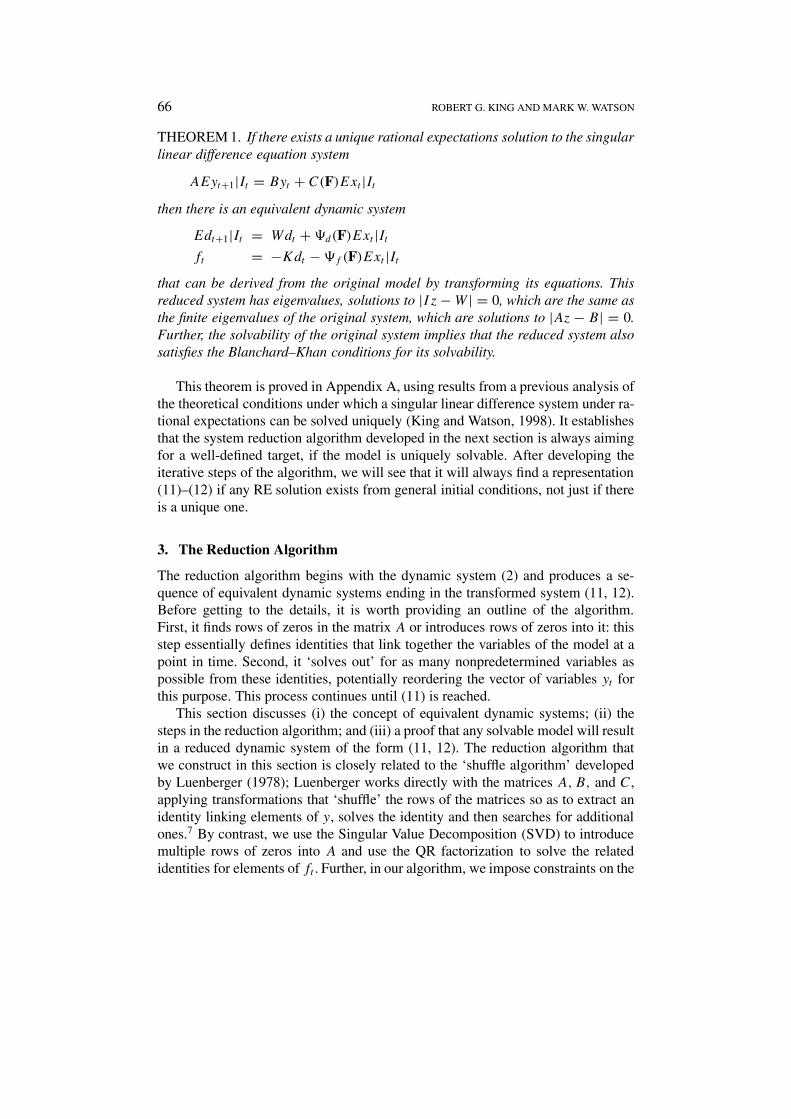
THEOREM 1. If there exists a unique rational expectations solution to the singularlinear difference equation system
AEyt+1|It = Byt + C(F)Ext |Itthen there is an equivalent dynamic system
Edt+1|It = Wdt + �d(F)Ext |Itft = −Kdt − �f (F)Ext |It
that can be derived from the original model by transforming its equations. Thisreduced system has eigenvalues, solutions to |Iz−W | = 0, which are the same asthe finite eigenvalues of the original system, which are solutions to |Az − B| = 0.Further, the solvability of the original system implies that the reduced system alsosatisfies the Blanchard–Khan conditions for its solvability.
This theorem is proved in Appendix A, using results from a previous analysis ofthe theoretical conditions under which a singular linear difference system under ra-tional expectations can be solved uniquely (King and Watson, 1998). It establishesthat the system reduction algorithm developed in the next section is always aimingfor a well-defined target, if the model is uniquely solvable. After developing theiterative steps of the algorithm, we will see that it will always find a representation(11)–(12) if any RE solution exists from general initial conditions, not just if thereis a unique one.
3. The Reduction Algorithm
The reduction algorithm begins with the dynamic system (2) and produces a se-quence of equivalent dynamic systems ending in the transformed system (11, 12).Before getting to the details, it is worth providing an outline of the algorithm.First, it finds rows of zeros in the matrix A or introduces rows of zeros into it: thisstep essentially defines identities that link together the variables of the model at apoint in time. Second, it ‘solves out’ for as many nonpredetermined variables aspossible from these identities, potentially reordering the vector of variables yt forthis purpose. This process continues until (11) is reached.
This section discusses (i) the concept of equivalent dynamic systems; (ii) thesteps in the reduction algorithm; and (iii) a proof that any solvable model will resultin a reduced dynamic system of the form (11, 12). The reduction algorithm thatwe construct in this section is closely related to the ‘shuffle algorithm’ developedby Luenberger (1978); Luenberger works directly with the matrices A,B, and C,applying transformations that ‘shuffle’ the rows of the matrices so as to extract anidentity linking elements of y, solves the identity and then searches for additionalones.7 By contrast, we use the Singular Value Decomposition (SVD) to introducemultiple rows of zeros into A and use the QR factorization to solve the relatedidentities for elements of ft . Further, in our algorithm, we impose constraints on the
SYSTEM REDUCTION AND SOLUTION ALGORITHMS 67
admissible transformations that rule out moving any of the predetermined variables(k) into f .
3.1. EQUIVALENT DYNAMIC SYSTEMS
The various systems produced by the system reduction algorithm are equivalent inthe sense that there is one-to-one transformation connecting them. Specifically, twotypes of transformations are used in the algorithm. The first type of transformationsinvolves non-singular matrices T and V designed to introduce rows of zeros intoA. That is: it transforms the equations (T ) and the variables (V ) of the model:
T [AF − B]V −1VEyt |It = T C(F)Ext |It ,to yield a new dynamic system of the form,
[A∗F − B∗]Ey∗t |It = C∗(F)Ext |It ,
with [A∗F−B∗] = T [AF−B]V −1, C∗(F) = T C(F), and new variables, Ey∗t |It =
V Eyt |It . Since T and V are non-singular, the transformation produces an equiv-alent system. Further, both the new system and the original system have the sameroots to their determinantal polynomials, since |A∗z − B∗| = |T ||Az − B||V −1|.The algorithm restricts V to simply reorder the variables so that the reduced di-mension system is in terms of the model’s original variables. The second set oftransformations are those of conventional system reduction. Section (2.3) showedhow this transformation could be summarized by multiplying the model’s equa-tions by a specific polynomial T (F) =GF + H , with two key properties. First,|T (z)| = τ = 0, so that again, this transformation does not alter the roots of themodel’s determinantal equation. Second, the matrices G and H are chosen so thatthe system remains first order.
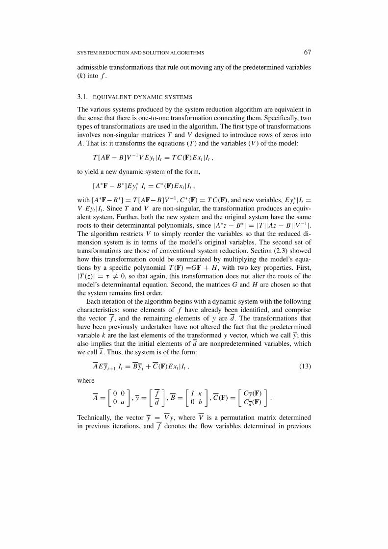
Each iteration of the algorithm begins with a dynamic system with the followingcharacteristics: some elements of f have already been identified, and comprisethe vector f , and the remaining elements of y are d. The transformations thathave been previously undertaken have not altered the fact that the predeterminedvariable k are the last elements of the transformed y vector, which we call y; thisalso implies that the initial elements of d are nonpredetermined variables, whichwe call λ. Thus, the system is of the form:
AEyt+1|It = Byt + C(F)Ext |It , (13)
where
A =[
0 00 a
], y =
[f
d
], B =
[I κ
0 b
], C(F) =
[Cf (F)Cd(F)
].
Technically, the vector y = V y, where V is a permutation matrix determinedin previous iterations, and f denotes the flow variables determined in previous
68 ROBERT G. KING AND MARK W. WATSON
iterations. The vector d is partitioned as d = (λ′
k′)′, so that the predeterminedvariables k always appear as the final n(k) elements. The iteration then proceedsby moving some of the elements of λ into f . The algorithm terminates when this isno longer possible. As we show below, the resulting value of a will be non-singularif the original system satisfies the restriction |Az − B| = 0 and a solution to themodel exists.
3.2. THE ALGORITHM STEPS
The algorithm includes five steps:
Step 1: Initialization
Begin by setting y = d = y, A = a = A, B = b = B, C(F) = Cd(F) = C(F) andCf (F) = 0. Since f is initially absent from the model, n(f ) = 0 and n(d) = n(y).If a is non-singular, proceed to Step 5, otherwise proceed to Step 2.
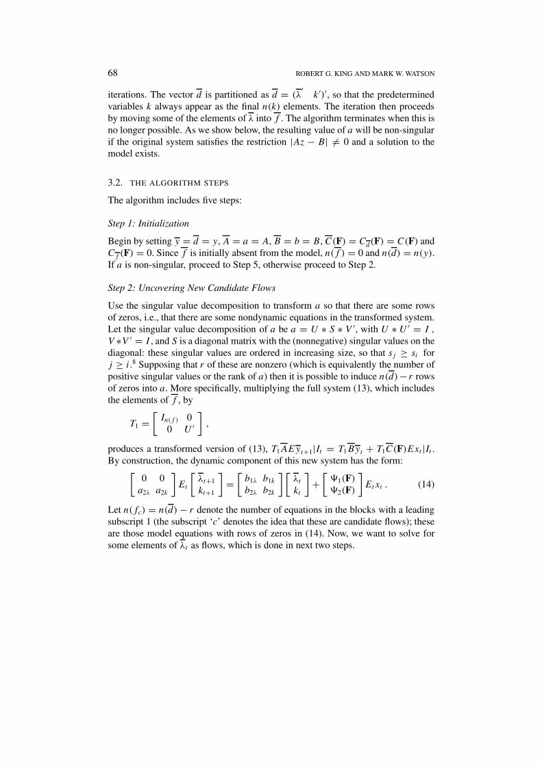
Step 2: Uncovering New Candidate Flows
Use the singular value decomposition to transform a so that there are some rowsof zeros, i.e., that there are some nondynamic equations in the transformed system.Let the singular value decomposition of a be a = U ∗ S ∗ V ′, with U ∗ U ′ = I ,
V ∗V ′ = I , and S is a diagonal matrix with the (nonnegative) singular values on thediagonal: these singular values are ordered in increasing size, so that sj ≥ si forj ≥ i.8 Supposing that r of these are nonzero (which is equivalently the number ofpositive singular values or the rank of a) then it is possible to induce n(d)− r rowsof zeros into a. More specifically, multiplying the full system (13), which includesthe elements of f , by
T1 =[In(f ) 0
0 U ′
],
produces a transformed version of (13), T1AEyt+1|It = T1Byt + T1C(F)Ext |It .By construction, the dynamic component of this new system has the form:[
0 0a2λ a2k
]Et
[λt+1
kt+1
]=
[b1λ b1k
b2λ b2k
][λtkt
]+
[�1(F)�2(F)
]Etxt . (14)
Let n(fc) = n(d) − r denote the number of equations in the blocks with a leadingsubscript 1 (the subscript ‘c’ denotes the idea that these are candidate flows); theseare those model equations with rows of zeros in (14). Now, we want to solve forsome elements of λt as flows, which is done in next two steps.

SYSTEM REDUCTION AND SOLUTION ALGORITHMS 69
Step 3: Isolating New Flows
Focusing on the first block of equations of (14): b1λλt + b1k kt = −�1(F)Etxt ,first determine the implied number of linearly independent restrictions on λt (callthis n(fn) for the number of new flows). Transform the equations and variablesso as to facilitate the solution of the equations using the QR factorization of b1λ:QR = b1λP .9 Since P is an n(λ) × n(λ) permutation matrix, this factorizationimplies that the elements of λt can be reordered by multiplying by P ′. Thus, forthe full vector y, the reordering is produced by:
V1 = I 0 0
0 P ′ 00 0 I
.
That is, rewrite the dynamic system T1AEyt+1|It = T1Byt + T1C(F)Ext |It asT1AEV −1
1 V1yt+1|It = T1BV −11 V1yt + T1C(F)Ext |It . While reordering λ, V1 pre-
serves the ordering of f and k. Also reorganize the system’s equations using theQR factorization of b1λ
T2 = I 0 0
0 Q′ 00 0 I
.
Hence, the transformations of the system through Step 2 are: T2T1AEV −11 V1yt+1|It
= T2T1BV−1
1 V1yt + T2T1C(F)Ext |It .
Step 4: Conventional System Reduction
It follows that there are n(fn) = rank(b1λ) new flows. Put alternatively, if n(f ) isthe number of pre-existing flows then the (n(f )+n(fn))× (n(f )+n(fn)) leadingsubmatrix of T2T1BV
−11 is of the form
Bff =[I 00 R11
],
where R11 is the (n(fn)) by (n(fn)) submatrix of the R matrix in the QR fac-torization of b1λ. The matrix is Bff is clearly invertible (since R11 is invertible)and, hence, we can employ the conventional system reduction procedure detailedin Section (2.3). This yields a new system in the form of (13), but with a smallermatrix a.
Step 5: Terminating the Iterative Scheme
If the resulting new value a is singular, then the sequence of Steps 2–4 is repeated.10
Otherwise, the resulting dynamic system is aEdt+1|It = bdt +Cd(F)Ext |It , whichcan be rewritten as Edt+1|It = Wdt + �d(F)Ext |It with W = a−1b and �d(F) =a−1Cd(F).

70 ROBERT G. KING AND MARK W. WATSON
3.3. CONVERGENCE OF THE ALGORITHM
We now establish that this algorithm will produce a non-singular reduced systemof the form (11) with p ≤ n(y) iterations, i.e., the construction and applicationof p transformations T (F) for equations and L (reordering transformations) forvariables. This results requires two conditions: (i) that there is a non-zero determi-nantal polynomial, |Az − B| = 0 for some z and (ii) that for every set of initialconditions (each vector k0) there exists a solution, i.e., there is a stochastic process{yt}∞
t=0 such that the equations of the original model are satisfied at each date.The first of these conditions is readily verifiable: it can be checked prior to
starting on the algorithm. The second of these conditions is an assumption, whichis discussed further below. The convergence result is stated formally as:
THEOREM 2. The singular linear difference equation system A Etyt+1 = B
yt + C(F) Etxt has an equivalent dynamic system representation comprised offt + K dt + �f (F) Etxt = 0 and Etdt+1 = Wdt + �d(F) Etxt , where f andd are vectors containing the elements of y, if: (i) the determinental polynomial,|Az−B|, is not zero for all values of z; and (ii) there exists a solution to the singularlinear difference equation system from every set of initial conditions k0. Further,the system reduction algorithm will compute this equivalent, reduced system in anumber of iterations p that is no more than the number of variables.
The theorem is proved as follows. First, note that each algorithm iteration involvesapplication of a matrix polynomial T (F) with nonzero determinant τ to the dy-namic system: this operation does not alter condition (i) since |Az−B| = 0 implies|A∗z − B∗| = |T (z)||Az − B| = τ |Az − B| = 0. Second, if {yt }∞
t=1 is a solutionto the original model, then it is also a solution to any transformed model obtainedvia such a T (F) operation. (If the original model implies A Etyt+1 − B yt − C(F)Etxt = 0 then application of T (F) = GF + H implies that A∗ Et yt+1 − B∗yt − T (F)C(F) Etxt = 0 with A∗F − B∗ = T (F)[AF − B] so that {yt}∞
t=1 is asolution to the transformed model.)
The next parts of the proof of the theorem involve details of the algorithm. Asstressed above, each iteration eliminates some elements of y from d and movesthem into f so long as it is possible to construct another T (F). Thus it is direct toestablish an upper bound on the number of algorithm iterations: with one or moreelements moved on each iteration, the algorithm must converge in less than n(y)
iterations.The construction of a T (F) at each iteration of the algorithm will be possible
unless n(fn) = 0 in Step 3, i.e., unless it is impossible to isolate one or more newflows. Since n(fn) = rank(b1λ), if n(fn) = 0 then this implies that the matrix b1λ
contains only zeros. That is, an equation of the transformed model is:
b1λλt + b1kkt = 0λt + b1kkt = �1(F)Etxt . (16)

SYSTEM REDUCTION AND SOLUTION ALGORITHMS 71
Now, suppose that, in addition b1k = 0: then there is a row of zeros in Az−B and,hence, 0 = |Az − B| = |Az − B|. In this equality, the first equality follows fromthe implied rows of zeros in T1A and T1B, and the second equality follows becausethe roots of the determinantal equation are unaltered by any of the transformationsused in the reduction algorithm. Thus, condition (i) is violated in this case. Thus,condition (i) implies b1k = 0 if b1λ = 0.11
On the other hand, if b1λ = 0 and b1k = 0, then b1kkt = �1(F)Etxt makes it ispossible to solve for a subset of the predetermined variables kt at each date t thatare a function of the other predetermined variables and a distributed lead of theexpected values of the xt ’s. This outcome violates condition (ii), since it imposesconstraints on the initial conditions for the predetermined variables. Hence, underconditions (i) and (ii), there cannot be an equation of the form (16). As a result,each successive iteration of the algorithm eliminates some new flows and ultimateconvergence is guaranteed.
The theorem of this section is useful for two related purposes. First, it providesa useful interpretation of the failure of the algorithm in Step 3 in the context ofa specific model: if the algorithm fails at this stage and it has been verified that|Az − B| = 0, then this failure implies that no solution of the model exists fromall initial conditions. Second, the theorem establishes that the algorithm can finda reduced dynamic system of the form (11, 12) even when there is not a unique,stable solution of the form studied by Blanchard and Kahn (1980) and King andWatson (1998). Since Theorem 2 only postulates a solution from a set of arbitraryinitial conditions, then the solution might include unstable dynamics of economicinterest (for example, unit roots) or it might involve a multiplicity of RE equilibriaalong the lines of Farmer (1993). Hence, Theorem 2 broadens the range of modelsto which the system reduction algorithm can be applied.
4. Solving the Model
After application of the system reduction algorithm, the transformed dynamicsystem takes the form:
ft = −[KfλKfk][λtkt
]− �f (F)Ext |It (17)
Et
[λt+1
kt+1
]=
[Wλλ Wλk
Wkλ Wkk
][λtkt
]+
[�λ(F)�k(F)
]Etxt . (18)
This is a nonsingular dynamic system of the form studied by Blanchard and Kahn(1980) and which is at the heart of the model solution approach in KPR-TA.
The solution of this model is discussed in three steps. First, the implications ofstability for the initial conditions on λt are determined. Second, the constructionof perfect foresight solutions is considered. Finally, dynamic decision rules areconstructed.

72 ROBERT G. KING AND MARK W. WATSON
4.1. INITIAL CONDITIONS ON λt
The treatment of the determination of the initial conditions on λt follows Blanchardand Kahn (1980). To begin, we let Vu be a (n(u) by n(d)) matrix that isolates theunstable roots of W .12 That is, Vu has the property that
VuW = µVu ,
where µ is a lower triangular (n(u) by n(u)) matrix with the unstable eigenvalueson its diagonal. Applying Vu to (18), then Vu Etdt+1 = Vu Wdt +Vu �d(F)Etxt =µ Vu dt + Vu�d(F)Etxt .13 The dynamics of ut = Vudt are then:
Etut+1 = µut + Vu�d(F)Etxt . (19)
This expression can be used to generate formulae for (a) perfect foresight solutions;and (b) Markov decision rules. In each case, ut is chosen so that there is a stablesystem despite the existence of unstable roots. Following Sargent (1979) and Blan-chard and Kahn (1980), this is accomplished by unwinding unstable roots forward.Practically, in the computer code discussed below, unstable roots are defined asfollows. Suppose that there is a discount factor, β. Then, a root µi is unstable ifβµi > 1. This version of the requirement allows us to treat unit roots as stable.14
The solutions for u can be used to uniquely determine the date t behaviorof the non-predetermined variables λt . As stressed by Blanchard–Kahn (1980)this requires that there be the same number of elements of u as there are non-predetermined variables. In terms of the condition ut = Vudt = Vuλλt + Vukkt ,this requirement means that we have an equal number of equations and unknowns.However, it is also the case that a unique solution mandates that the (square) matrixVuλ is of full rank. This condition on Vuλ is an implication of the more general rankcondition that Boyd and Dotsey (1993) give for higher order linear rational expec-tations models. Essentially, the rank condition rules out matrices W with unstableroots associated with the predetermined variables rather than nonpredeterminedvariables.
4.2. PERFECT FORESIGHT (SEQUENCE) SOLUTIONS
Perfect foresight solutions, i.e., the response of the economy to a specifiedsequence of x : {xs}∞
s=t , are readily constructed. Expression (19) implies that:
ut = −[I − µ−1F]−1[µ−1Vu�d(F)]Etxt . (20)
Call the result of evaluating the right-hand side of this expression ut = �u(F)Etxt .Then, ut = Vuλλt + Vuλkt, implies that the initial condition on λt is
λt = −V −1uλ Vukkt + V −1
uλ �u(F)Etxt . (21)
With knowledge of λt , expressions (17) and (18) imply that:
ft = −[Kfk − KfλV−1uλ Vuk]kt − [KfλV
−1uλ �u(F) + �f (F)]Etxt (22)
SYSTEM REDUCTION AND SOLUTION ALGORITHMS 73
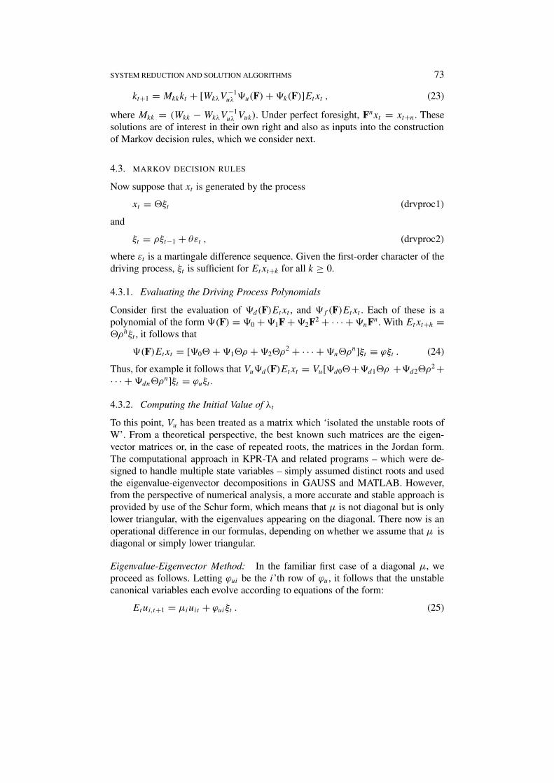
kt+1 = Mkkkt + [WkλV−1uλ �u(F) + �k(F)]Etxt , (23)
where Mkk = (Wkk − WkλV−1uλ Vuk). Under perfect foresight, Fnxt = xt+n. These
solutions are of interest in their own right and also as inputs into the constructionof Markov decision rules, which we consider next.
4.3. MARKOV DECISION RULES
Now suppose that xt is generated by the process
xt = ?ξt (drvproc1)
and
ξt = ρξt−1 + θεt , (drvproc2)
where εt is a martingale difference sequence. Given the first-order character of thedriving process, ξt is sufficient for Etxt+k for all k ≥ 0.
4.3.1. Evaluating the Driving Process Polynomials
Consider first the evaluation of �d(F)Etxt , and �f (F)Etxt . Each of these is apolynomial of the form �(F) = �0 + �1F + �2F2 + · · · + �nFn. With Etxt+h =?ρhξt , it follows that
�(F)Etxt = [�0? + �1?ρ + �2?ρ2 + · · · + �n?ρ
n]ξt ≡ ϕξt . (24)
Thus, for example it follows that Vu�d(F)Etxt = Vu[�d0?+�d1?ρ +�d2?ρ2 +
· · · + �dn?ρn]ξt = ϕuξt .
4.3.2. Computing the Initial Value of λt
To this point, Vu has been treated as a matrix which ‘isolated the unstable roots ofW’. From a theoretical perspective, the best known such matrices are the eigen-vector matrices or, in the case of repeated roots, the matrices in the Jordan form.The computational approach in KPR-TA and related programs – which were de-signed to handle multiple state variables – simply assumed distinct roots and usedthe eigenvalue-eigenvector decompositions in GAUSS and MATLAB. However,from the perspective of numerical analysis, a more accurate and stable approach isprovided by use of the Schur form, which means that µ is not diagonal but is onlylower triangular, with the eigenvalues appearing on the diagonal. There now is anoperational difference in our formulas, depending on whether we assume that µ isdiagonal or simply lower triangular.
Eigenvalue-Eigenvector Method: In the familiar first case of a diagonal µ, weproceed as follows. Letting ϕui be the i’th row of ϕu, it follows that the unstablecanonical variables each evolve according to equations of the form:
Etui,t+1 = µiuit + ϕuiξt . (25)
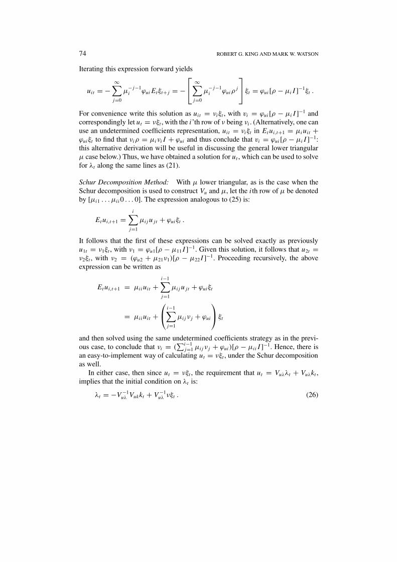
74 ROBERT G. KING AND MARK W. WATSON
Iterating this expression forward yields
uit = −∞∑j=0
µ−j−1i ϕuiEtξt+j = −
∞∑
j=0
µ−j−1i ϕuiρ
j
ξt = ϕui[ρ − µiI ]−1ξt .
For convenience write this solution as uit = νiξt , with vi = ϕui[ρ − µiI ]−1 andcorrespondingly let ut = νξt , with the i’th row of ν being νi . (Alternatively, one canuse an undetermined coefficients representation, uit = νiξt in Etui,t+1 = µiuit +ϕuiξt to find that νiρ = µiνiI + ϕui and thus conclude that vi = ϕui[ρ − µiI ]−1:this alternative derivation will be useful in discussing the general lower triangularµ case below.) Thus, we have obtained a solution for ut , which can be used to solvefor λt along the same lines as (21).
Schur Decomposition Method: With µ lower triangular, as is the case when theSchur decomposition is used to construct Vu and µ, let the ith row of µ be denotedby [µi1 . . . µii0 . . . 0]. The expression analogous to (25) is:
Etui,t+1 =i∑
j=1
µij ujt + ϕuiξt .
It follows that the first of these expressions can be solved exactly as previouslyu1t = ν1ξt , with ν1 = ϕu1[ρ − µ11I ]−1. Given this solution, it follows that u2t =ν2ξt , with ν2 = (ϕu2 + µ21ν1)[ρ − µ22I ]−1. Proceeding recursively, the aboveexpression can be written as
Etui,t+1 = µiiuit +i−1∑j=1
µij ujt + ϕuiξt
= µiiuit + i−1∑
j=1
µij νj + ϕui
ξt
and then solved using the same undetermined coefficients strategy as in the previ-ous case, to conclude that νi = (
∑i−1j=1 µij νj + ϕui)[ρ − µiiI ]−1. Hence, there is
an easy-to-implement way of calculating ut = νξt , under the Schur decompositionas well.
In either case, then since ut = νξt , the requirement that ut = Vuλλt + Vuλkt ,implies that the initial condition on λt is:
λt = −V −1uλ Vukkt + V −1
uλ νξt . (26)

SYSTEM REDUCTION AND SOLUTION ALGORITHMS 75
4.3.3. Solutions for the Other Variables
With knowledge of this solution for λt , expressions (17) and (18) imply that:
ft = [Kfk − KfλV−1uλ Vuk]kt + [KfλV
−1uλ ν + ϕf ]ξt (27)
kt+1 = Mkkkt + [WkλV−1uλ ν + ϕk]ξt , (28)
where Mkk = (Wkk − WkλV−1uλ Vuk) as above and ϕf and ϕk are the evaluations of
the �f and �k polynomials (as in (24)).
4.3.4. The RE Solution in State Space Form
These solutions can be grouped together with other information to produce a statespace system, i.e., a pair of specifications Zt = FSt and St+1 = M St + Net+1.The specific form is:
ftλtktxt
=
[Kfk − KfλV−1uλ Vuk] [KV −1
uλ ν + ϕf ]−V −1
uλ Vuk V −1uλ ν
I 00 ?
[ktξt
](29)
[kt+1
ξt+1
]=
[Mkk [WkλV
−1uλ ν + ϕk]
0 ρ
] [ktξt
]+
[0θ
]εt+1 . (30)
Further, given
[ftdt
]= Lyt , it is easy to restate this representation in terms of the
original ordering of the variables.
4.4. HOW IT WORKS IN PRACTICE
The algorithms described above are available in MATLAB and GAUSS.15 In eachcase, the researcher specifies the dynamic system of the form (2), specifying thematrices A,B, [C0 . . . Cl]; the location of the predetermined variables in the vectoryt ; and the number of leads l in the C polynomial. The researcher also specifies thedriving process (4.3, 4.3). The programs return a solution in the state space form(29, 30), which makes it easy to compute impulse responses, spectra, populationmoments and stochastic simulations. This solution is also a convenient one forestimation and model evaluation.
We make it easy for the researcher to check the necessary condition for modelsolvability, |Az − B| = 0. If the model solution package fails when this conditionis satisfied, it must then be for one of two other reasons:
(1) the reduction algorithm terminates without reaching a solution. In our ex-perience, this failure has nearly always meant that the model is misspecified, most

76 ROBERT G. KING AND MARK W. WATSON
likely as a result of a programming error, so that new flows cannot be isolated. Veryoccasionally, we have included a behavioral equation of the form,
b1λλt + b1kkt = eλt + b1kkt = −�1(F)Etxt ,
where e is a very small number or a vector containing zeros and very small num-bers. Then, we must decide whether e = 0 so that the model is not solvable or toadjust tolerance values to treat this as an equation to be solved for some new flows.
(2) the model solution algorithms reports the wrong number of unstable rootsrelative to the number of predetermined variables. After excluding the possibilitythat the locations of the predetermined variables has been erroneously specified,there are two remaining possibilities. First, stability is defined in our code in arelative rather than absolute sense: an adjustment of the critical value for stability,the parameter β, may be necessary. Second, the model may actually not have anRE equilibrium or there may be a multiplicity of equilibria.16
5. Extension to Timing Models
An important class of macroeconomic models views the discrete time period t asdivided into subperiods that are distinguished by differing information sets. Forexample, analyses of the real effects of monetary disturbances in flexible pricemodels frequently make such assumptions, as in Svensson (1985) or Christianoand Eichenbaum (1992). An extension of the approach outlined above can be usedfor these models as well.17 Thus, consider the a generic timing model in the form:
A0Eyt+1|I0t + A1Eyt+1|I1t + · · · + AJEyt+1|IJ t= B0Eyt |I0t + B1Eyt |I1t + · · · + BJEyt |IJ t+C0(F)Ext |I0t + C1(F)Ext |I1t + · · · + CJ (F)Ext |IJ t ,
(31)
where I0t is no current information, IJ t is full current information, and the infor-mation sets are ordered as increasing in information (I0 ⊂ I1t . . . ⊂ Ijt . . . ⊂ IJ t ).
In this expression, as earlier in this article, F is the lead operator defined so as toshift the dating of the variable but not of the information set, so that Cj(F)Ext |Ijtrepresents the distributed lead C0jExt+1|Ijt+C1jExt+1|Ijt+· · ·+CJjExt+J |Ijt .18
There is a simple two-stage strategy for solving such timing models. First, onesolves a common information model that is derived by conditioning on I0t : thissolution is straightforward given the results in this paper and constitutes the harderpart of the RE solution. Second, one uses that solution to solve for the influencesof the particular timing model under study.
SYSTEM REDUCTION AND SOLUTION ALGORITHMS 77
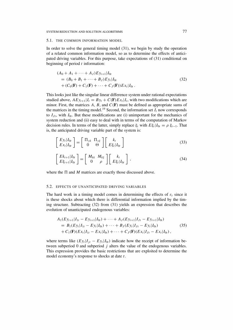
5.1. THE COMMON INFORMATION MODEL
In order to solve the general timing model (31), we begin by study the operationof a related common information model, so as to determine the effects of antici-pated driving variables. For this purpose, take expectations of (31) conditional onbeginning of period t information:
(A0 + A1 + · · · + AJ )Eyt+1|I0t
= (B0 + B1 + · · · + BJ )Eyt |I0t
+ (C0(F) + C1(F) + · · · + CJ (F))Ext |I0t .
(32)
This looks just like the singular linear difference system under rational expectationsstudied above, AEyt+1|It = Byt + C(F)Ext |It , with two modifications which areminor. First, the matrices A, B, and C(F) must be defined as appropriate sums ofthe matrices in the timing model.19 Second, the information set It now correspondsto IJ t , with I0t . But these modifications are (i) unimportant for the mechanics ofsystem reduction and (ii) easy to deal with in terms of the computation of Markovdecision rules. In terms of the latter, simply replace ξt with Eξt |I0t = ρ ξt−1. Thatis, the anticipated driving variable part of the system is:[
Eyt |I0t
Ext |I0t
]=
[Fyk Fyξ
0 ?
] [kt
Eξt |I0t
](33)
[Ekt+1|I0t
Eξt+1|I0t
]=
[Mkk Mkξ
0 ρ
][kt
Eξt |I0t
], (34)
where the F and M matrices are exactly those discussed above.
5.2. EFFECTS OF UNANTICIPATED DRIVING VARIABLES
The hard work in a timing model comes in determining the effects of εt since itis these shocks about which there is differential information implied by the tim-ing structure. Subtracting (32) from (31) yields an expression that describes theevolution of unanticipated endogenous variables:
A1(Eyt+1|I1t − Eyt+1|I0t ) + · · · + AJ (Eyt+1|IJ t − Eyt+1|I0t )
= B1(Eyt |I1t − Eyt |I0t ) + · · · + BJ (Eyt |IJ t − Eyt |I0t )
+C1(F)(Ext |I1t − Ext |I0t ) + · · · + CJ (F)(Ext |IJ t − Ext |I0t ) ,
(35)
where terms like (Eyt |Ijt − Eyt |I0t ) indicate how the receipt of information be-tween subperiod 0 and subperiod j alters the value of the endogenous variables.This expression provides the basic restrictions that are exploited to determine themodel economy’s response to shocks at date t .

78 ROBERT G. KING AND MARK W. WATSON
It is useful if these restrictions are written in the following ‘one subperiod aheadinnovation’ form:
A1(Eyt+1|I1t − Eyt+1|I0t ) + · · · + AJ(Eyt+1|IJ t − Eyt+1|IJ−1,t )
= B1(Eyt |I1t − Eyt |I0t ) + · · · + BJ (Eyt |IJ t − Eyt |IJ−1,t )
+C1(F)(Ext |I1t − Ext |I0t ) + · · · + CJ (F)(Ext |IJ t − Ext |IJ−1,t ) ,
(36)
where Aj = (Aj +· · ·+AJ ); Bj = (Bj +· · ·+BJ ); and Cj(F) = (Cj(F)+· · ·+CJ (F)).
This expression implies that we can concentrate on finding the solution to
Aj(Eyt+1|Ijt − Eyt+1|Ij−1,t )
= Bj (Eyt |Ijt − Eyt |Ij−1,t )
Cj (F)(Ext |Ijt − Ext |Ij−1,t )
(37)
for each j = 1, 2, . . . J .
5.2.1. Solving for the Effects of Shocks in Subperiod j
This subsection discusses how to use (37) to determine the effects of shocks in sub-period j . It is useful to partition the vector y into parts that are nonpredetermined
(K) and parts that are predetermined (k). That is, write y =[K
k
].
Since kt is predetermined, it does not respond to shocks within any of the sub-periods j of period t . Hence, the term Bj(Eyt |Ijt −Eyt |Ij−1,t ) in (37) simplifies toBj,K(EKt |Ijt −EKt |Ij−1,t ), where Bj,K involves the relevant columns of Bj . Fur-ther, from (34), Eyt+1|Ijt = E[Eyt+1|I0,t+1]|Ijt = FykEkt+1|Ijt + FyξEξt+1|Ijtand Eξt+1|Ijt = ρEξt |Ijt = ρ(ρξt−1 +θEεt |Ijt ) given the driving process in (4.3)above. Accordingly, it follows that:
Aj(Eyt+1|Ijt − Eyt+1|Ij−1,t )
= AjFyk(Ekt+1|Ijt − Ekt+1|Ij−1,t )
+AjFyξρθ(Eεt |Ijt − Eεt |Ij−1,t ) .
(38)
Since Cj(F) = Cj,0 + Cj,1F + · · · +Cj,pFp, it is direct that Cj(F)(Ext |Ijt −Ext |Ij−1,t ) = (Cj,0? + Cj,1?ρ+ · · · +Cj,p?ρ
p) (Eεt |Ijt − Eεt |Ij−1,t ): call thissolution �j(Eεt |Ijt − Eεt |Ij−1,t ).
Combining these results, (37) can be written as:
[ −Bj,K AjFyk
] [EKt |Ijt − EKt |Ij−1,t
Ekt+1|Ijt − Ekt+1|Ij−1,t
]= [
�j − AjFyρθ] [Eεt |Ijt − Eεt |Ij−1,t
].
(39)
Solving (39), determines the variables at t as functions of shocks, taking as givenaspects of the future solution (as provided by Fyk and Fyξ ).

SYSTEM REDUCTION AND SOLUTION ALGORITHMS 79
What is known about subperiod j that is useful in considering the solution to(39)? The specification of the economic problem shows which variables have beendetermined in subperiods prior to j , i.e., which elements of
qjt =[
EKt |Ijt − EKt |Ij−1,t
Ekt+1|Ijt − Ekt+1|Ij−1,t
]are zero by the structure of the model. Further, the model also supplies theinformation that is revealed in the subperiod, i.e., Eεt |Ijt − Eεt |Ij−1,t .
From a mathematical point of view, (39) contains more equations (n(y)) thanunknowns since some of the elements of qjt are determined prior to subperiodj . This is accommodated as follows. First, write (39) as Mqjt = N(Eεt |Ijt −Eεt |Ij−1,t ) and use the fact that there is a permutation matrix Pq which makes thefirst p elements of qjt the predetermined ones.20 Second, translate the system to:(M P ′
q)(Pqqjt ) = N(Eεt |Ijt−Eεt |Ij−1,t ). Third, partition M ≡ M P ′q as [M1M2],
with the first p columns of M being those that are attached to the predeterminedvariables, q1
j t , and the last n(y) − p columns being those attached to the variablesdetermined in subperiod j and later, q2
j t . Thus, the system takes the form:
M2q2j t = N(Eεt |Ijt − Eεt |Ij−1,t ) .
This system is n(y) equations in n(y)−p unknowns, which are coefficients ηj thatdescribe how the elements of q2
j t respond to the shocks Eεt |Ijt − Eεt |Ij−1,t . Thissystem can be solved using the QR factorization, checking in the process that thereis indeed a consistent solution (by determining that the last p rows of Q′N are allzeros, where Q is the lead matrix in the QR factorization of M2).
Proceeding similarly through subperiods j = 1, 2, . . . J yields a matrix η:[Kt − EKt |I0t
kt+1 − Ekt+1|I0t
]= η(εt − Eεt |I0t ) ,
where η contains many zeros due to the subperiod structure. Partition this matrixas:
η =[ηKηk
]and use these matrices in augmenting the solutions for the anticipated components.The overall solution for the observable variables is thus:[
ytxt
]=
[Fyk Fyξ
0 ?
] [kt
ρξt−1
]+
[ηy0
]εt ,
where ηy =[ηK0
]with the last lines of zeros corresponding to the elements of k.
The predetermined variables and driving variables evolve according to:[kt+1
ξt+1
]=
[Mkk Mkξ
0 ρ
] [kt
ρξt−1
]+
[ηk0
]εt +
[0I
]εt+1

80 ROBERT G. KING AND MARK W. WATSON
These equations may easily be placed in a state space form. The observables evolveaccording to:
zt =[ytxt
]=
[Fyk Fyξρ ηy
0 ?ρ ?
] kt
ξt−1
εt
and the states evolve according to: kt+1
ξtεt+1
=
Mkk Mkξρ ηk
0 ρ I
0 0 0
kt
ξt−1
εt
+
0
0I
εt+1 .
6. Conclusions
In this article, we described an algorithm for the reduction of singular linear differ-ence systems under rational expectations of the form (1) and alternative algorithmsfor the solution of the resulting reduced dimension system. We also described anextension to ‘timing models’, i.e., to variants of (1) with distinct informationalsubperiods. This set of methods is flexible and easy to use.
Appendix: Proof of Theorem 1
The proof relies on results in King and Watson (1998). That paper developed theconditions under which singular linear difference system can be uniquely solvedunder rational expectations. There were two necessary and sufficient conditions.First, |Az − B| = 0 for some z. Second, a particular matrix VUK had full rank:this matrix requirement was necessary to link non-predetermined variables K tounstable canonical variables U , where the definition of unstable canonical variablescontained both finite and infinite eigenvalues. For the convenience of a readermaking the transition from King and Watson (1998), the notation in this sectionfollows that paper and not the main text.
Begin with the solvable dynamic system written in a canonical form employedin King and Watson (1998):21
(A∗F − B∗)V Etyt = C∗Etxt ,
where V is a variable transformation matrix and
[A∗F − B∗] =[(NF − I ) 0
0 (FI − J )
].
with N being a nilpotent matrix.22 King and Watson (1998, particularly Ap-pendix A) show that such an equivalent system can always be constructed for

SYSTEM REDUCTION AND SOLUTION ALGORITHMS 81
any model that possesses a unique, stable rational expectations solution. Thetransformed variables in this canonical form are[
Ut
st
]≡
it
utst
= V Etyt
with the partition defined by the magnitude of the eigenvalues. First, there are asmany elements of s as there are stable eigenvalues of J . Second, there are as manyelements of it as there are columns of N . As explained in King and Watson (1998),these are canonical variables associated with ‘infinite’ eigenvalues.
The intuition behind the proof of Theorem 1 is that the infinite canonical vari-ables, it , of King and Watson (1998) are governed by dynamic identities and,consequently, can be related to the ft variables of the present article. Once thisrelationship is established and exploited to eliminate the ft , the remaining variablesdt are governed by a reduced dimension dynamic system that depends on ut , st inthe same way as the original model.
Linking it and ft
Premultiplication of the canonical dynamic system by
η(F) =[(NF − I )−1 0
0 I
]results in[
I 00 (FI − J )
]V Etyt = η(F)C∗Etxt .
Now, partition the transformation of variables matrix V as follows
V =[Vif Vid
Vδf Vδd
]=
Vif Viλ Vik
Vuf Vuλ Vuk
Vsf Vsλ Vsk
,
using the notation d ′ = [λ′k′] to denote the dynamic variables and δ′ = [u′s′]. Let
VUK =[Vif Viλ
Vuf Vuλ
].
where λ are those elements K left after the removal of ft that are thus part of thedynamic vector d. Without loss of generality, we will assume that the elements ofy are ordered so that Vif is square and nonsingular. This is always possible giventhat VUK is nonsingular.
Using the first partitions of V , the dynamic system can be written[Vif Vid
(FI − J )Vδf (FI − J )Vδd
]Etyt = η(F)C∗Etxt .

82 ROBERT G. KING AND MARK W. WATSON
Notice that there are no lead operators in the first n(i) = n(f ) rows of thistransformed system.
Construction of Reduced System
Now we proceed to construct a reduced dimension dynamic system. To accomplishthis, we premultiply by a matrix polynomial T (F) that is partitioned as[
T11(F) T12(F)T21(F) T22(F)
]with components that satisfy:
T11(F)Vif + T12(F)(FI − J )Vδf = I
T11(F)Vid + T12(F)(FI − J )Vδd = K
T21(F)Vif + T22(F)(FI − J )Vδf = 0
T21(F)Vid + T22(F)(FI − J )Vδd = [FI − W ] ,where K and W are unknown matrices.
The first two of these conditions may be used to set
T11(F) = V −1if
T12(F) = 0
which jointly imply that K = V −1if Vid .
Employing the third and fourth condition together
T22(F){(FI − J )[Vδd − Vδf V−1if Vid]} = FI − W .
Standard results on the determinants and inverses of partitioned matrices imply thatV = [Vδd − Vδf V
−1if Vid] is an invertible matrix. Accordingly, this condition may
be satisfied with
T22(F) = V −1
and
W = V −1J V .
A further implication is then that
T21(F) = −V −1(FI − J )Vδf V−1if .
Hence, it follows that
T (F) =[
V −1if 0
−V −1(FI − J )Vδf V−1if V −1
]
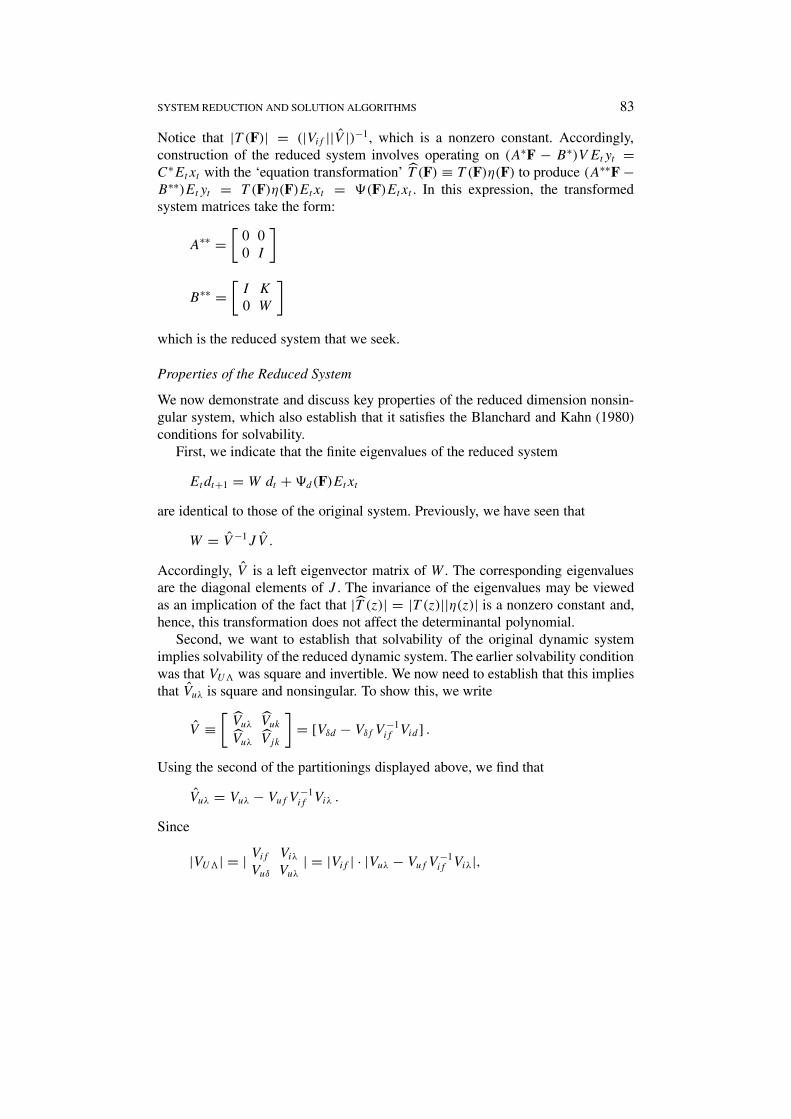
SYSTEM REDUCTION AND SOLUTION ALGORITHMS 83
Notice that |T (F)| = (|Vif ||V |)−1, which is a nonzero constant. Accordingly,construction of the reduced system involves operating on (A∗F − B∗)VEtyt =C∗Etxt with the ‘equation transformation’ T (F) ≡ T (F)η(F) to produce (A∗∗F −B∗∗)Etyt = T (F)η(F)Etxt = �(F)Etxt . In this expression, the transformedsystem matrices take the form:
A∗∗ =[
0 00 I
]
B∗∗ =[I K
0 W
]
which is the reduced system that we seek.
Properties of the Reduced System
We now demonstrate and discuss key properties of the reduced dimension nonsin-gular system, which also establish that it satisfies the Blanchard and Kahn (1980)conditions for solvability.
First, we indicate that the finite eigenvalues of the reduced system
Etdt+1 = W dt + �d(F)Etxt
are identical to those of the original system. Previously, we have seen that
W = V −1J V .
Accordingly, V is a left eigenvector matrix of W . The corresponding eigenvaluesare the diagonal elements of J . The invariance of the eigenvalues may be viewedas an implication of the fact that |T (z)| = |T (z)||η(z)| is a nonzero constant and,hence, this transformation does not affect the determinantal polynomial.
Second, we want to establish that solvability of the original dynamic systemimplies solvability of the reduced dynamic system. The earlier solvability conditionwas that VUK was square and invertible. We now need to establish that this impliesthat Vuλ is square and nonsingular. To show this, we write
V ≡[Vuλ Vuk
Vuλ Vjk
]= [Vδd − Vδf V
−1if Vid ] .
Using the second of the partitionings displayed above, we find that
Vuλ = Vuλ − VufV−1if Viλ .
Since
|VUK| = | Vif Viλ
Vuδ Vuλ| = |Vif | · |Vuλ − VufV
−1if Viλ|,
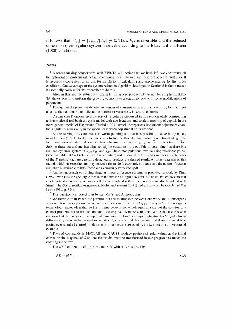
84 ROBERT G. KING AND MARK W. WATSON
it follows that |Vuλ| = |VUK|/|Vif | = 0. Thus, Vuλ is invertible and the reduceddimension (nonsingular) system is solvable according to the Blanchard and Kahn(1980) conditions.
Notes
1 A reader making comparisons with KPR-TA will notice that we have left two constraints onthe optimization problem rather than combining them into one and therefore added a multiplier. Itis frequently convenient to do this for simplicity in calculating and approximating the first orderconditions. One advantage of the system reduction algorithm developed in Section 3 is that it makesit essentially costless for the researcher to do this.
Also, in this and the subsequent example, we ignore productivity trends for simplicity. KPR-TA shows how to transform the growing economy to a stationary one with some modifications ofparameters.
2 Throughout the paper, we denote the number of elements in an arbitrary vector wt by n(w). Wealso use the notation ns to indicate the number of variables s in several contexts.
3 Crucini (1991) encountered the sort of singularity discussed in this section while constructingan international real business cycle model with two locations and costless mobility of capital. In themore general model of Baxter and Crucini (1993), which incorporates investment adjustment costs,the singularity arises only in the special case when adjustment costs are zero.
4 Before leaving this example, it is worth pointing out that it is possible to solve it ‘by hand’,as in Crucini (1991). To do this, one needs to first be flexible about what is an elment of ft . Thefirst three linear equations above can clearly be used to solve for ct , pt , and λ1t as functions of λ2t .Solving these out and manipulating remaining equations, it is possible to determine that there is areduced dynamic system in λ2t , k1t , and k2t . These manipulations involve using relationships be-tween variables at t +1 (elements of the A matrix) and relationships between variables at t (elementsof the B matrix) that are carefully designed to produce the desired result. A further analysis of thismodel, which stresses the interplay between the model’s economic structure and the nature of systemreduction is available at http://people.bu.edu/rking/kwre/irbc2.pdf
5 Another approach to solving singular linear difference systems is provided in work by Sims(1989), who uses the QZ-algorithm to transform the a singular system into an equivalent system thatcan be solved recursively. All models that can be solved with our technology can also be solved withSims’. The QZ-algorithm originates in Moler and Stewart (1971) and is discussed by Golub and VanLoan (1989, p. 394).
6 This question was posed to us by Kei Mu Yi and Andrew John.7 We thank Adrian Pagan for pointing out the relationship between our work and Luenberger’s
work on ‘descriptor systems’, which are specifications of the form Ayt+1 = Byt+Cxt . Luenberger’sterminology makes clear that he has in mind systems for which equilibria are not the solution to acontrol problem, but rather contain some ‘descriptive’ dynamic equations. While this accords withour view that the analysis of ‘suboptimal dynamic equilibria’ is a major motivation for ‘singular lineardifference systems under rational expectations’, it is worthwhile stressing that there are benefits toposing even standard control problems in this manner, as suggested by the two location growth modelexample.
8 The svd commands in MATLAB and GAUSS produce positive singular values as the initialentries on the diagonal of S so that the results must be transformed in our programs to match theordering in the text.
9 The QR factorization of a p × m matrix M with rank r is given by
QR = MP , (15)

SYSTEM REDUCTION AND SOLUTION ALGORITHMS 85
where P is an m by m permutation matrix (i.e., P can be constructed by reordering the rows of Im);Q is a p by p unitary matrix; and R is a p by m matrix such that
R =[R11 R12
0 0
].
where R11 is an r by r upper diagonal, nonsingular matrix and R12 is an r by (m − r) matrix.The QR factorization is useful because it allows us to solve the equation system My = N for
r of the elements of y in terms of the remaining (m − r) elements of y and the parameters N . Thatis, we can write the equation My = N as RP ′y = Q′N and partition P ′y = [y′
1y′2]′. Then, the
solution is y1 = R−111 (G1 − R12y2), where G1 is the first r rows of Q′M . The equation system is
consistent only if G2 = 0, where G2 is the last (m − r) rows of Q′N .10 The matrix a is not necessarily nonsingular because because we may have solved for a smaller
number of new flows than actual flows. Or, in some cases, the transformations that eliminate someflows may themselves induce new singularities. To see this latter point, consider the example
pt = λt−Etpt+1 + Etλt+1 = pt − xt
The associated 2 × 2 A matrix has rank 1, so that the first step is to eliminate pt = λt . But when oneuses this implication, the resulting 1 × 1 a matrix is 0, so that it has rank 0. The resulting reducedsystem involves no dynamic variables, but is simply the pair of equations pt = xt and λt = xt .
11 Luenberger (1978) uses an argument like this one to establish the inevitable convergence of his‘shuffle’ algorithm when |Az − B| = 0.
12 Notice that the eigenvalue-eigenvector or Schur decomposition may involve complex numbers.At the same time, the resulting rational expectations solutions are constrained to involve real numbersonly. As a double check, our computer programs test for the presence of non-negligible imaginarycomponents.
13 One interpretation of this transformation is that ut = Vudt is the vector of unstable canonicalvariables and that Vu is the matrix of left eigenvectors that corresponds to the unstable eigenvalues;in this case, µ is a Jordan matrix with the entries below the main diagonal corresponding to repeatedunstable roots. However, a better computational method is to use the Schur decomposition. In thiscase µ is a lower triangular matrix with the unstable eigenvalues on the diagonal.
14 It is also consistent with the implications of transversality conditions in dynamic optimizingmodels, where the requirement is typically that β1/2µi > 1.
15 The core programs in GAUSS and MATLAB as well as many example applications are availableat http://people.bu.edu/rking/kwre.html.
16 Given the nature of our reduction algorithm, it is fairly straightforward to calculate restric-tions that rational expectations imposes on the solution of the reduced system, Etdt+1 = Wdt +�d(F)Etxt , in the case of multiple equilibria. But we have not yet written code for this purpose.
17 This approach was employed in King and Watson (1996) to study the empirical implications offinancial market frictions models in the style of Christiano and Eichenbaum (1992).
18 We make use of the fact that IJ t = I0,t+1 in some of the derivations below.19 We assume that this common information model is solvable in the sense discussed above. This
requires that |Az−B| = 0, which may be verified prior to the solution of the model in question, andalso that additional ‘rank’ conditions are satisfied, which are verified during the solution process.
20 These are not the same matrices M and N which enter in the state equations.21 For the theoretical characterization of solutions and the purposes of this appendix, the restriction
to only current xt is immaterial. This is because its is the properties of A and B that govern theproperties of the solutions and the existence of a reduced dimension dynamic subsystem.
86 ROBERT G. KING AND MARK W. WATSON
22 A nilpotent matrix has zero elements on and below its main diagonal, with zeros and onesappearing abitrarily above the diagonal. Accordingly, there is a number l such that Nl is a matrixwith all zero elements.
References
Baxter, Marianne and Crucini, Mario J. (1993). Explaining saving-investment correlations. AmericanEconomic Review, 83(3), 416-436.
Blanchard, Olivier J. and Kahn, Charles (1980). The solution of linear difference models underrational expectations. Econometrica, 48(5), 1305–1311.
Boyd, John H. III and Dotsey, Michael (1993). Interest rate rules and nominal determinacy. FederalReserve Bank of Richmond, Working Paper, revised February 1994.
Christiano, Lawrence J. and Eichenbaum, Martin (1992). Liquidity effects and the monetarytransmission mechanism. American-Economic-Review 82(2), 346–353.
Crucini, Mario (1991). Transmission of business cycles in the open economy. Ph.D. dissertation,University of Rochester.
Farmer, Roger E.A. (1993). The Macroeconomics of Self-Fulfilling Prophecies, MIT Press.Golub, G.H. and Van Loan, C.F. (1989). Matrix Computations, 2nd edn., Johns Hopkins University
Press, Baltimore.King, R.G., Plosser, C.I., and Rebelo, S.T. (1988a). Production, growth and business cycles, I: The
basic neoclassical model. Journal of Monetary Economics, 21(2/3), 195–232.King, R.G., Plosser, C.I., and Rebelo, S.T. (1988b). Production, growth and business cycles, technical
appendix. University of Rochester Working Paper.King, R.G. and Watson, M.W. (1996). Money, interest rates, prices and the business cycle. Review of
Economics and Statistics.King, R.G. and Watson, M.W. (1998). The solution of singular linear difference systems under
rational expectations. IER.King, R.G. and Watson, M.W. (1995a). The solution of singular linear difference systems under
rational expectations. Working Paper.King, R.G. and Watson, M.W. (1995b). Research notes on timing models.Luenberger, David (1977). Dynamic equations in descriptor form. IEEE Transactions on Automatic
Control, AC-22(3), 312–321.Luenberger, David, (1978). Time invariant descriptor systems. Automatica, 14(5), 473–480.Luenberger, David (1979). Introduction to Dynamic Systems: Theory, Models and Applications, John
Wiley and Sons, New York.McCallum, Bennett T. (1983). Non-uniqueness in rational expectations models: An attempt at
perspective. Journal of Monetary Economics, 11(2), 139–168.Moler, Cleve B. and Stewart, G.W. (1973). An algorithm for generalized matrix eigenvalue problems.
SIAM Journal of Numerical Analysis, 10(2), 241–256.Sargent, Thomas J. (1979). Macroeconomic Theory. Academic Press, New York.Sims, Christopher A. (1989). Solving non-linear stochastic optimization problems backwards.
Discussion Paper 15, Institute for Empirical Macroeconomics, FRB Minneapolis.Svensson, Lars E.O. (1985). Money and asset prices in a cash in advance economy. Journal of
Political Economy, 93, 919–944.