Neutrino mass bound in the standard scenario for

supernova electronic antineutrino emission

G. Pagliaroli

INFN, Laboratori Nazionali del Gran Sasso, Assergi (AQ), ItalyICTP, Strada Costiera 11, I-34014 Trieste, Italy

F. Rossi-Torres

Instituto de F́ısica “Gleb Wataghin” - UNICAMP, 13083-970 Campinas SP, BrazilINFN, Laboratori Nazionali del Gran Sasso, Assergi (AQ), Italy

F. Vissani

INFN, Laboratori Nazionali del Gran Sasso, Assergi (AQ), ItalyICTP, Strada Costiera 11, I-34014 Trieste, Italy

Abstract

Based on recent improvements of the supernova electron antineutrino emis-sion model, we update the limit on neutrino mass from the SN1987A datacollected by Kamiokande-II, IMB and Baksan. We derive the limit of 5.8 eVat 95% CL, that we show to be remarkably insensitive to the astrophysicaluncertainties. Also we evaluate the ultimate mass sensitivity of this methodfor a detector like Super-Kamiokande. We find that the bound lies in thesub-eV region, 0.8 eV at 95 % CL being a typical outcome, competitive withthe values that are presently probed in laboratory. However, this bound issubject to strong statistical fluctuations, correlated to the characteristics ofthe first few events detected. We briefly comment on the prospects offeredby future detectors.

INFN preprint LNGS/TH-01/10

1. Introduction

The interest in measuring the, presently unknown, absolute mass scaleof neutrinos has been renewed by the experimental evidences of neutrino

Preprint submitted to Elsevier February 5, 2010

oscillation [1, 2].

It is known since long [3] that neutrinos from supernova can contributevaluable information on the mass of neutrinos. In fact, the stringent limit ofmν < 5.7 eV at 95 % CL has been obtained by Loredo and Lamb [4] usingSN1987A neutrinos [5, 6, 7]; another important result in this connection isthe one obtained by Nardi and Zuluaga, who argue that future supernovawill permit us to probe the sub-eV region [8, 9, 10].

In the present paper, we aim at updating both these results: namely, weimprove the bound on neutrinos from SN1987A and we evaluate the ultimatesensitivity of the method to probe neutrino masses introduced by Zatsepin.

2. The limit from SN1987A

2.1. The reasons of an updated analysis

The limit from SN1987A [4] is quoted in the PDG report but it is consid-ered “no longer comparable with the limits from tritium beta decay” [11]. Infact, in the 3 neutrino context it can be compared with the limit obtained inlaboratory [12, 13]; the value of the latter is 2 eV, about three times tighterthan the former.

Nevertheless, the analysis on neutrino mass of Lamb and Loredo [4] main-tains a big methodological merit, being the only one based on a theoreticallymotivated model for the emission of neutrinos. Their model is capable ofreproducing the expected (main) features of neutrino emission and, in par-ticular, it includes an initial phase of intense luminosity. This phase, calledaccretion, is the crucial ingredient for theories that attempt to explain theexplosion of the star, based on the “delayed scenario” [14, 15]–see [16] for areview. As we will show in the following, this phase is the theoretical ingredi-ent that allowed to obtain the comparably strong limit on the mass recalledpreviously.

There are two specific considerations that make a reanalysis necessary:1) it has been noted that the likelihood function adopted by Lamb and Loredohas a statistical bias [17]; 2) in addition, an improved model for the emissionof neutrinos (which overcomes certain shortcomings and involves significantchanges in the astrophysical parameters resulting from SN1987A data anal-ysis) has been recently introduced in the scientific literature [18, 19].

2

2.2. Procedure of analysis

The method used in this paper to investigate the neutrino mass is basedon punctual comparison between the features of the collected data [5, 6, 7]and the expectations resulting from a specific theoretical model [18, 19].This model describes the expected flux of electron antineutrinos, taking intoaccount that the main reaction leading to observable events is ν̄ep → e+nboth in water Cherenkov than in scintillator detectors.

We assume that the shape of the flux is known up to nine free parametersthat are obtained fitting the data. Let us explain their meaning: The firstsix parameters belong to two emission phases (accretion and cooling) and areused to take into account the large astrophysical uncertainties. Each emissionphase is characterized by its intensity, its duration and the average energyof the emitted neutrinos. The three parameters of the accretion phase arethe initial mass (Ma), the time scale (τa) and the initial temperature (Ta);those of the cooling phase are the radius (Rc), the time scale (τc) and theinitial temperature (Tc). For details and analytical expressions see [18, 19].The other three parameters are called “offset times”; each one of them is theabsolute delay of the first observed event in each detector, more explicitlydescribed below. We need to include three different offset times because theclocks of Kamiokande-II, IMB and Baksan were not synchronized [5, 7].

Now we include the effects of neutrino mass. The antineutrino flux,Φν̄e(t, Eν), is a parametric function that depends on the time of emission(t) and on the energy of the antineutrino (Eν), see in particular Eqs. 10, 13,19 and 20 in reference [18]. Of course this function must vanish for t ≤ 0.Using the same notation of ref. [18] (see in particular Eq. 8 there) we canwrite the emission time for the i-th event as follow:

ti = δti + toff −∆ti. (1)

The first term in the right hand side, δti, is the relative time between thei-th and the first observed event in the considered detector, which is knowndirectly from the data without significant error. The second one, toff, isthe offset time parameter which is the sum of the emission time of the firstneutrino detected, t1, and of its delay due to the velocity of propagation,

3

∆t1, namely toff = t1 + ∆t1. Finally, the last term,

∆ti =D

2c

(mν

Eν,i

)2

, (2)

is the delay of the neutrino due to a non-zero mass [3], where D is thedistance of propagation. The neutrino energy Eν,i of the i-th event can bereconstructed from the measured energy of the positron, Ei, which is knownup to its error, δEi. The numerical value of the delay when D = 50 kpc (asfor SN1987A), Eν = 10 MeV (a typical value) and mν = 10 eV is ∆t = 2.6s, which is five times longer than the duration of the phase of accretion.

The scope of the statistical analysis is to extract from the fit toff and mν

at the same time. It is quite evident that these two terms work in oppositesense, see Eq. (1) and recall the condition ti ≥ 0. This makes the extractionof these two parameters more difficult, especially in the case of SN1987A,when the number of observed events is small. We adopt the same likelihoodfunction L constructed in [18] including in it the expression for the timesti given in Eq. (1). This is a function of 10 parameters, namely the nineparameters previously discussed plus the neutrino mass.

2.3. Results and remarks

Using the definition L = exp(−χ2/2) we obtain the function that allowsus to estimate the neutrino mass

∆χ2(mν) = χ2(mν)− χ2best fit, (3)

This function is plotted in Fig. 1. The two continuous curves show the resultsof SN1987A data analysis. The thick line is obtained, for any fixed value ofthe neutrino mass, maximizing the likelihood with respect to the other 9free parameters. The curve is somewhat bumpy, reflecting the presence ofmultiple maxima that compete in the likelihood with similar height. Theexistence of these maxima has been already remarked in [18] and causes nu-merical difficulties. To avoid these problems we bound the mass of accretingmaterial Ma, which regulates the intensity of neutrinos emission in the ac-cretion phase, to be lower than 0.6 M� [4, 18]. The thin line, instead, ariseswhen the 6 astrophysical parameters are set to the best-fit values obtainedin [18]. In this case only the 3 offset times are allowed to fluctuate freelyto maximize the likelihood. The comparison of the two curves reveals someinteresting features:

4

0 2 4 6 8mΝ@eVD

1

2

3

4

5

6

7DΧ

2

Figure 1: The curves show various ∆χ2(mν) obtained by analyzing supernova neu-trino data as a function of the neutrino mass. The two continuous curves areobtained from SN1987A data; the thick one includes the astrophysical uncertain-ties, the thin one assumes instead that the astrophysical parameters of neutrinoemission are known. For comparison, we include the result of the analysis of sim-ulated data set, collected in a detector a la Super-Kamiokande (SK), for a futuresupernova exploding at 10 kpc from us (leftmost dashed curve). This curve, dis-cussed in detail later, illustrates the ultimate sensitivity of the method.

• In spite of the really different assumptions, namely the complete knowl-edge of the supernova ν̄e emitted flux or only of its shape (up to 6parameters), the two curves are quite similar. This shows that thelarge uncertainties in the astrophysics of the emission are not the mainlimitation in this type of analysis.

• In both curves, the minimum is located at mν 6= 0, however, thisis not statistically significant.1 This is linked to a clustering of theevents #1,2,4,6 of Kamiokande-II for mν ∼ 3.5 eV, already remarkedby several authors, e.g., [21].

From our statistical analysis, we obtain as limit on neutrino mass fromSN1987A data the value

mν < 5.8 eV at 95% CL. (4)

1We note that the presentation using mν rather than m2ν–which is the quantity that is

actually probed, see Eq. (1)–emphasizes somewhat artificially the region close to mν ∼ 0.

5

As already noted, this does not change much if we assume that the astro-physics of the emission is perfectly known; in this case, in fact, the limitbecomes mν < 5.6 eV at 95% CL: see Fig. 1.

From Eqs. (1) and (2) and from the previous discussion, it is quite evidentthat the information on the presence of the neutrino mass is mainly containedin the earlier events and, in particular, in those with low energy. Theseconsiderations select, as the most relevant data, the six events collected byKamiokande-II in the first second [5], that incidentally, are also the mostrelevant ones to determine the presence of an accretion phase [4, 18].

3. The sensitivity of the method

These findings led us to the question of evaluating the ultimate sensi-tivity of this method for a future galactic supernova event. For this aim,we will analyze in this section simulated data, extracted from the generatordescribed in [19] upgraded to describe the propagation of massive neutrinos,focussing mostly on the possibilities of the existing detectors. We will in-troduce and critically examine the assumptions used to derive the bound,comment on their statistical meaning, and overview the prospects offered byfuture detectors.

3.1. Statistical procedure

The expected counting rate of the signal is a function of the emissiontime t, neutrino energy Eν , detector mass Md, distance of the supernova Dand of the astrophysical parameters that describe the electron antineutrinoemission, namely

R(t, Eν) = 6.7× 1031 Md

1 ktonσν̄ep(Eν)Φ̃ν̄e(t, Eν)ε(Ee+), (5)

that depends on the supernova distance through the electron antineutrinoflux, i.e., Φν̄e ∝ 1/D2. We will consider a SN exploding at a distance ofD = 10 kpc, typical of a galactic event [22, 23]. Here, σν̄ep(Eν) is the crosssection of the interaction process [24]; the function ε(Ee+) is the detectorefficiency that we set to 98% above a threshold of 6.5 MeV; we approximateEe = Eν −∆ with ∆ = 1.293 MeV.

6

0.00 0.05 0.10 0.15 0.20t@secD

10

20

30

40

50Evis@MeVD

0.00 0.05 0.10 0.15 0.20t@secD

10

20

30

40

50Evis@MeVD

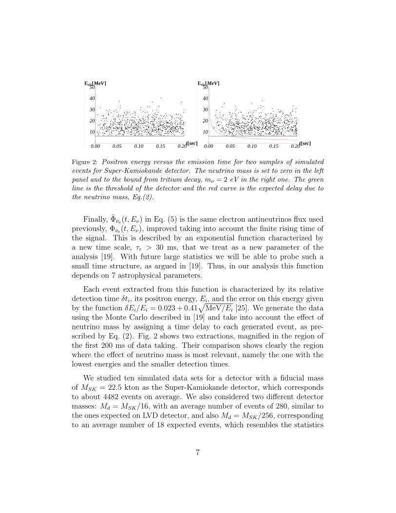
Figure 2: Positron energy versus the emission time for two samples of simulatedevents for Super-Kamiokande detector. The neutrino mass is set to zero in the leftpanel and to the bound from tritium decay, mν = 2 eV in the right one. The greenline is the threshold of the detector and the red curve is the expected delay due tothe neutrino mass, Eq.(2).

Finally, Φ̃ν̄e(t, Eν) in Eq. (5) is the same electron antineutrinos flux usedpreviously, Φν̄e(t, Eν), improved taking into account the finite rising time ofthe signal. This is described by an exponential function characterized bya new time scale, τr > 30 ms, that we treat as a new parameter of theanalysis [19]. With future large statistics we will be able to probe such asmall time structure, as argued in [19]. Thus, in our analysis this functiondepends on 7 astrophysical parameters.

Each event extracted from this function is characterized by its relativedetection time δti, its positron energy, Ei, and the error on this energy givenby the function δEi/Ei = 0.023 + 0.41

√MeV/Ei [25]. We generate the data

using the Monte Carlo described in [19] and take into account the effect ofneutrino mass by assigning a time delay to each generated event, as pre-scribed by Eq. (2). Fig. 2 shows two extractions, magnified in the region ofthe first 200 ms of data taking. Their comparison shows clearly the regionwhere the effect of neutrino mass is most relevant, namely the one with thelowest energies and the smaller detection times.

We studied ten simulated data sets for a detector with a fiducial massof MSK = 22.5 kton as the Super-Kamiokande detector, which correspondsto about 4482 events on average. We also considered two different detectormasses: Md = MSK/16, with an average number of events of 280, similar tothe ones expected on LVD detector, and also Md = MSK/256, correspondingto an average number of 18 expected events, which resembles the statistics

7

collected for SN1987A.

We calculate the bound on the mass by assuming that:

• The astrophysical parameters are precisely known; we use those inref. [18], that agree with the expectations of a standard collapse andset τr = 50 ms.

• The offset time is known without significant error (more discussionlater).

These are very optimistic assumptions as appropriate to evaluate the ultimatesensitivity of the method. We discuss the weight of these assumptions in thefollowing and their implications on the understanding of SN1987A results.

We note in passing that the neutrino mass enters the likelihood throughEq. (2), in the form m2

νD; moreover, the interaction rate in Eq. (5) dependson the combination Md/D

2: thus, the likelihood obeys the exact scaling law

L(Md, D,mν) = L(α2Md, αD,mν/√α). (6)

This means, e.g., that once we know the value of the neutrino mass boundfor Md = MSK/16, we get the bound for Md = MSK and D = 40 kpc simplyhalving it. From here, we also conclude that the bound on the mass canbe written as mν < f(Md/D

2)/ 4√Md, where the function f depends on the

selected statistical level on the adopted test and on the specific data set.

3.2. Results and discussion

The 95% CL neutrino mass bounds, obtained with fixed astrophysicalparameters, are reported in Fig. 3 for each analyzed data set.

The case of low statistics and SN1987A. As first step, we discuss the dia-monds points corresponding to a detector with mass Md = MSK/256. Theaverage number of events in this case is very similar to the one observed forSN1987A, so we can explore the fluctuations due to the features of the datain a small data set. The values of the neutrino mass bound fall in the intervalof 1.6 eV < mν < 6.4 eV showing that each particular data set contains verydifferent information about the neutrino mass presence.

8

ææ

æ

æ

ææ

æ

æ

æ

æ

àààà

à

ààà

à

à

ì

ì

ì

ìì

ì

ì

ì

ì

ì

10 30 100 300 1000 3000Nev

0.5

1.0

2.5

5.0

10.

mΝ@eVD

Figure 3: The dots represent the 95% CL bounds on neutrino mass from the analysisof simulated data; for each of the three value of the average numbers of expectedevents we extracted and analyzed 10 simulated data set. Circles (dots in the right),squares (center) and diamonds (left) correspond to the results in detectors withmasses Md = MSK , MSK/16 and MSK/256, respectively. The continuous anddashed curves describe the bounds given by Eq. (10) and discussed in the text.

We used these simulations to investigate the weight of the various as-sumptions of the analysis on the resulting bound. For a typical simulateddata set, we analyzed the data using three different procedures:

1. We suppose to know all the astrophysical parameters without errorsand also the offset time. In other words, the only free parameter ofthe likelihood is the neutrino mass. The resulting 95% CL on neutrinomass in this case is: mν < 4.4 eV.

2. We suppose that the offset time is unknown, whereas the 7 astrophysicalparameters are known from the theory. Namely, the likelihood is afunction of the neutrino mass and of the offset time. The resulting95% CL on neutrino mass in this case is: mν < 7.2 eV.

3. Finally, we suppose that we do not know any of the 9 parameters.Namely, only the shape of the signal in known from the theory andall parameters have to be estimated from the likelihood analysis. Theresulting 95% CL on neutrino mass in this case is: mν < 7.4 eV.

This study shows that the knowledge of the offset time significantly affectsthe value of the mass bound. Instead the comparison of the last two resultsconfirms that the knowledge of the astrophysical parameters is less criticalfor the analysis, in agreement with what we found for SN1987A data analysis.

9

We are ready for the comparison with the SN1987A results. This ispossible using the scaling relation of Eq. (6). Using α = 5, we translate therange 1.6 − 6.4 eV in the range 0.7 eV < mν < 2.9 eV when D = 50 kpcand for a detector mass Md 'MKII . For a fair comparison, we still need totake into account that the offset times and the astrophysical parameters areunknown in SN1987A analysis. So, comparing mν < 4.4 eV and mν < 7.4eV, we multiply this range by the factor 7.4/4.4 obtaining 1.2 eV < mν <4.9 eV. The bound from SN1987A, mν < 5.8 eV, is not far from this range.The residual difference can be attributed to the better performances of thesimulated detector. In fact, the improved efficiency implies that more eventsare collected at low energies; moreover, any misidentification of events isforbidden by constructions, due to the postulated absence of backgroundevents above the detection threshold.

The case of high statistics and the ultimate upper limit. Now we discuss theresults for high statistic, i.e., the case when Md = MSK , chosen to representthe observation of a future galactic supernova event. A typical simulateddata set is the one shown in the left panel of Fig. 2; the resulting ∆χ2 is theone given by the dashed line of Fig. 1, that implies:

mν < 0.8 eV at 95% CL (7)

This result confirms the possibility to probe the sub-eV region for neutrinomass using SNe neutrinos, in agreement with the finding of Nardi and Zulu-aga [8, 9, 10]. Also it would be closer to the sensitivity of about 0.2 eV thatwill be probed by the Katrin experiment [20].

An inspection of Fig. 3 shows also quite clearly that the bounds fluctuatestrongly with the individual simulation, even for high statistics. This can beexplained as follows. The emission time of each signal event is subject to thecondition ti > 0 (see Eq. (1)), which implies the condition on the neutrinomass:

mν < m∗ν = Mini

{Eν,i

√toff + δtiD/(2c)

}. (8)

When we replace Eν,i = Ei+ ∆, namely, neglecting the error in the measure-ment of the positron energy, we obtain the bound m∗

ν on the neutrino mass

10

Nev toff(ms) mν(eV) m∗ν(eV)

4328 4.9 0.78 0.944479 2.9 0.82 0.684497 2.9 0.72 0.764473 2.9 1.10 1.104492 4.6 0.84 0.774464 2.9 0.82 0.734488 3.5 0.90 0.724412 2.6 0.82 0.654412 1.2 0.59 0.524399 3.0 1.01 0.77

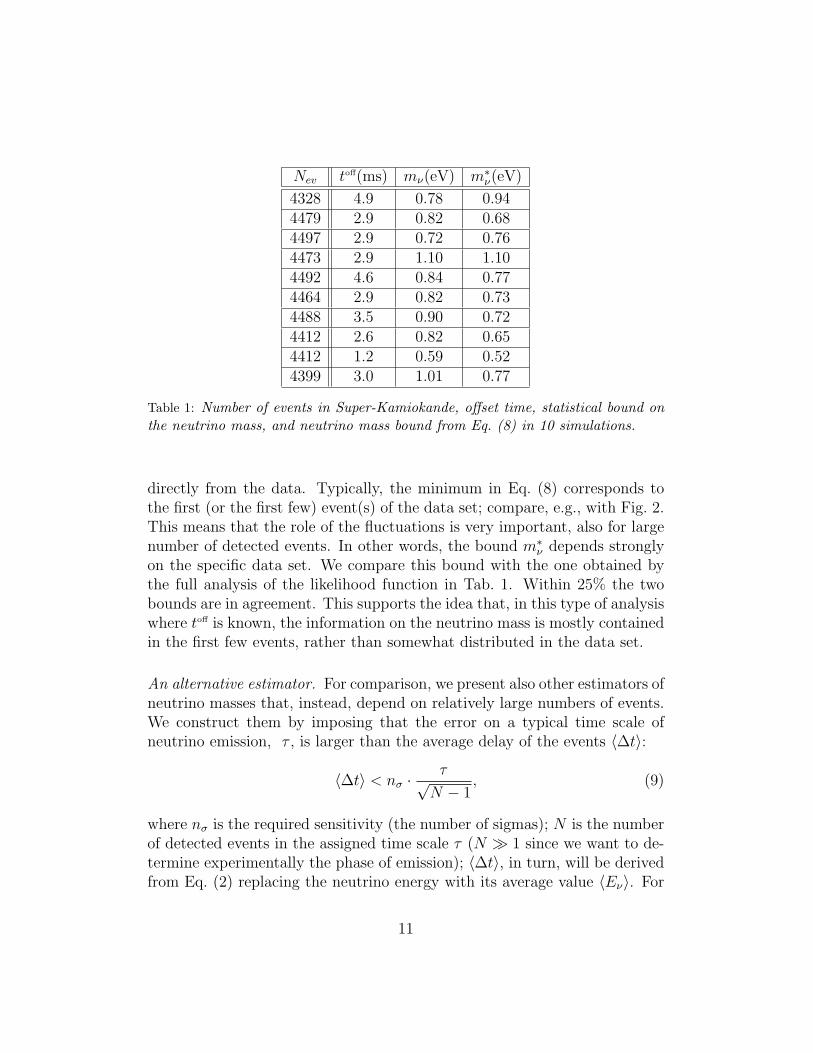
Table 1: Number of events in Super-Kamiokande, offset time, statistical bound onthe neutrino mass, and neutrino mass bound from Eq. (8) in 10 simulations.

directly from the data. Typically, the minimum in Eq. (8) corresponds tothe first (or the first few) event(s) of the data set; compare, e.g., with Fig. 2.This means that the role of the fluctuations is very important, also for largenumber of detected events. In other words, the bound m∗

ν depends stronglyon the specific data set. We compare this bound with the one obtained bythe full analysis of the likelihood function in Tab. 1. Within 25% the twobounds are in agreement. This supports the idea that, in this type of analysiswhere toff is known, the information on the neutrino mass is mostly containedin the first few events, rather than somewhat distributed in the data set.

An alternative estimator. For comparison, we present also other estimators ofneutrino masses that, instead, depend on relatively large numbers of events.We construct them by imposing that the error on a typical time scale ofneutrino emission, τ , is larger than the average delay of the events 〈∆t〉:

〈∆t〉 < nσ ·τ√N − 1

, (9)

where nσ is the required sensitivity (the number of sigmas); N is the numberof detected events in the assigned time scale τ (N � 1 since we want to de-termine experimentally the phase of emission); 〈∆t〉, in turn, will be derivedfrom Eq. (2) replacing the neutrino energy with its average value 〈Eν〉. For

11

a similar proposal, see [26]. Setting nσ = 2, we get the following bound onthe neutrino mass:

mν <2〈Eν〉

4√N − 1

√τ

D/c(10)

We use the value 〈Eν〉 = 13 MeV and D = 10 kpc for numerical purposes andconsider two concrete times scales of emission: the one of the accretion phase,τ = τa = 0.55 s, which corresponds to N = 0.4Nev; the one of the risingfunction, τ = τr = 50 ms, which corresponds instead to N = Nev/40. Theselead to the continuous curve and to the dashed curve of Fig. 3, respectively.As soon the expected number of events is large enough (N � 1), we geta stabler bound on the neutrino mass.2 However, Fig. 3 shows clearly thatthese are very conservative upper bounds, when compared with the truebounds from the full likelihood analysis.

The gravity wave trigger and its limitations. An important remark is in or-der. We evaluated the ultimate sensitivity of the method with the existingneutrino detectors, assuming that the offset time was known without signif-icant error. How can we achieve this? In principle, we could profit of thedetection of gravity waves, assuming they will be seen. However, two addi-tional conditions should be fulfilled: a precise location of the supernova inthe sky is needed; the interval of time between the onsets of gravitationaland neutrino emissions should be known. The first condition is needed ifthe detectors of gravity waves and of neutrinos are not in the same location.Elastic scattering neutrino events can provide such an information, but witha uncertainty of several ms [19], while an astronomical identification wouldmake this error negligible. The second condition has at present an associatedtheoretical 1σ error of about 1 ms [19], which is already limiting the sensitiv-ity of the existing neutrino detectors: see Tab. 1, or consider that IceCUBEuses 2 ms time window. In summary, the key condition for a successfulsearch for neutrino mass by this method is the possibility to implement veryprecise measurements of the time; however, the previous discussion showedthe difficulties to realistically surpass the millisecond time scale. It will be

2Note that in this limit and considering that the number of events scales as 1/D2, thebound in Eq. (10) is independent from the distance. The same occurs with the bound inEq. (8) if toff + δti ∝ D/

√Md, that is satisfied for an initial linear rise of the interaction

rate, R(t) ' ξtMd/D2 (which is the quantity that determines the time of the events).

12

important to take into account these considerations for an analysis of futurereal data, for instance, taking into account the errors on the measurement oftime. Another way to go beyond these limitations would be to rely on largersamples of data; this will be possible by future detectors, which leads us tothe last point of the discussion.

Future prospects. Finally, we comment on the prospects to improve the reachof this method to investigate neutrino masses. A straightforward possibilitywould be to use a bigger detector, say of megaton mass; note incidentally thatthis is mentioned already in the paper of Zapsepin [3]. For example, with anincrease of the number of events expected in Super-Kamiokande (22.5 ktonfiducial volume) by a factor of ∼ 20 one could expect an improvement on m2

ν

as the inverse of the square root of this number, thus reaching mν ≤ 0.4 eVin the most optimistic case. If instead we use the stabler bound of Eq. (10),we find again a value close to the one in Eq. (7).

An alternative possibility would be to identify the very short burst fromearly neutronization; see [27] for an earlier discussion. Its detection couldpermit us to investigate neutrino masses of similar size. In the standard sce-nario of neutrino emission, however, this burst leads to a very small fractionof the total number of events, which leads us again to consider a megatonwater Cherenkov detector. In fact, the elastic scattering events are 1/35 ofthe total sample; the burst comprises some 1/20 of the total energy releasedin νe’s, which, when converted in νµ,τ ’s by oscillations, have a cross section6.5 times smaller. Thus, a conservative estimation of the event fraction fromthe neutronization burst is 1/4500, which means about N =20 (=1) eventsin 450 (22.5) kton of fiducial volume from a supernova at nominal distance of10 kpc. If used in Eq. (10) with τ = 3 ms, this yields mν ≤ 0.7 eV, which isagain similar to the bound of Eq. (10), but possibly more stable and withoutresorting to the gravity wave trigger.3

3For a more precise bound one should keep into account that the elastic scatteringreaction νe→ νe does not allow to reconstruct the neutrino energy precisely.

13

4. Summary

The present work, part of a series of papers on supernova neutrinos [17,18, 19, 22, 24], was devoted to derive and discuss the bound on neutrinomass from supernova electron antineutrinos. Our bound, Eq. (4), agrees wellwith the one obtained by Lamb and Loredo [4], despite the large number ofdifferences in the procedures of analysis.

We argued that the result from SN1987A is relatively insensitive to thedetails of the emission model, as soon as the emission resembles the expec-tations of the standard scenario, that includes an initial phase of intenseantineutrino luminosity. We showed that the knowledge of the time whenneutrino emission begins (‘offset time’) has, instead, a significant impact onthe bound that the existing detectors can obtain.

We derived the ultimate sensitivity that can be provided by supernovaneutrinos with existing detectors. We showed that on average it lies in the in-teresting sub-eV region. However the key role of the first few detected eventsalso implies a large fluctuation on the mass bounds. A crucial requirementis the need to reach very precise measurements of the offset time; we arguedthat the detection of a gravity wave burst could permit to reach the sub-eVsensitivity with the existing neutrino detectors. We briefly commented on theprospect to improve the bound using future, megaton class, water Cherenkovdetectors.

References

[1] Proceedings of the CLXX Enrico Fermi Course “Measurements of Neu-trino Masses”, eds. C. Brofferio, F. Ferroni, F. Vissani, SIF-IOS, 2009.

[2] A. Strumia and F. Vissani, “Neutrino masses and mixings and...,”arXiv:hep-ph/0606054 and subsequent updates; G.L. Fogli, E. Lisi,A. Marrone and A. Palazzo, Prog. Part. Nucl. Phys. 57 (2006) 742;M.C. Gonzalez-Garcia and M. Maltoni, Phys. Rept. 460 (2008) 1.

[3] G.T. Zatsepin, Pisma Zh. Eksp. Teor. Fiz. 8 (1968) 333.

[4] T.J. Loredo and D.Q. Lamb, Phys. Rev. D 65 (2002) 063002.

14

[5] K.S. Hirata et al., Phys. Rev. D 38 (1988) 448; K. Hirata et al.[Kamiokande-II Collaboration], Phys. Rev. Lett. 58 (1987) 1490.

[6] R.M. Bionta et al., Phys. Rev. Lett. 58 (1987) 1494; C.B. Bratton et al.[IMB Collaboration], Phys. Rev. D 37 (1988) 3361.

[7] E.N. Alekseev, L.N. Alekseeva, V.I. Volchenko and I.V. Krivosheina,JETP Lett. 45 (1987) 589; E.N. Alekseev, L.N. Alekseeva,I.V. Krivosheina and V.I. Volchenko, Phys. Lett. B 205 (1988) 209.

[8] E. Nardi and J.I. Zuluaga, Phys. Rev. D 69 (2004) 103002.

[9] E. Nardi and J.I. Zuluaga, Nucl. Phys. B 731 (2005) 140.

[10] J.I. Zuluaga, PhD thesis defended on 2005 at the Univ. de Antioquia,Medellin, astro-ph/0511771v2.

[11] C. Amsler et al. [Particle Data Group], Phys. Lett. B 667 (2008) 1.

[12] C. Weinheimer et al., Phys. Lett. B 460 (1999) 219.

[13] A.I. Belesev et al., Phys. Lett. B 350 (1995) 263.

[14] D.K. Nadyozhin, Astrophys. Space Sci. 53 (1978) 131.

[15] H.A. Bethe and J.R. Wilson, Astrophys. J. 295 (1985) 14.

[16] H.T. Janka, Astronomy and Astrophysics, 368 (2001) 527; H.T. Janka,K. Langanke, A. Marek, G. Martinez-Pinedo and B. Mueller, Phys.Rept. 442 (2007) 38.

[17] A. Ianni, G. Pagliaroli, A. Strumia, F.R. Torres, F.L. Villante andF. Vissani, Phys. Rev. D 80 (2009) 043007.

[18] G. Pagliaroli, F. Vissani, M.L. Costantini and A. Ianni, Astropart. Phys.31 (2009) 163.

[19] G. Pagliaroli, F. Vissani, E. Coccia and W. Fulgione, Phys. Rev. Lett.103 (2009) 031102.

[20] J. Wolf [KATRIN Collaboration], arXiv:0810.3281 [physics.ins-det].

[21] H. Huzita, Mod. Phys. Lett. A 2 (1987) 905.

15

[22] M.L. Costantini, A. Ianni and F. Vissani, Nucl. Phys. Proc. Suppl. 139(2005) 27.

[23] A. Mirizzi, G.G. Raffelt and P.D. Serpico, JCAP 0605 (2006) 012.

[24] A. Strumia and F. Vissani, Phys. Lett. B 564 (2003) 42.

[25] M. Nakahata et al. [Super-Kamiokande Collaboration], Nucl. Instrum.Meth. A 421 (1999) 113.

[26] J.F. Beacom and P. Vogel, Phys. Rev. D 58 (1998) 093012.

[27] N. Arnaud, M. Barsuglia, M.A. Bizouard, F. Cavalier, M. Davier,P. Hello and T. Pradier, Phys. Rev. D 65 (2002) 033010.

16