Aspects of NeutrinoPhysics in the EarlyUniversePh.D. Thesis

Steen HannestadInstitute of Physics and AstronomyUniversity of AarhusOctober 1997

ContentsPreface v1 Introduction 11.1 Neutrinos . . . . . . . . . . . . . . . . . . . . . . . . . . . . . . . 11.2 Primordial Nucleosynthesis . . . . . . . . . . . . . . . . . . . . . 21.3 Thesis Outline . . . . . . . . . . . . . . . . . . . . . . . . . . . . 72 Particle Dynamics in the Expanding Universe 92.1 Global Evolution Equations . . . . . . . . . . . . . . . . . . . . . 92.2 The Boltzmann Equation . . . . . . . . . . . . . . . . . . . . . . 143 Basic Big Bang Nucleosynthesis 193.1 Theory . . . . . . . . . . . . . . . . . . . . . . . . . . . . . . . . . 193.2 Observations . . . . . . . . . . . . . . . . . . . . . . . . . . . . . 224 Dirac and Majorana Neutrino Interactions 294.1 De�nition and Properties of Neutrino Fields . . . . . . . . . . . . 304.2 Neutrino Weak Interactions . . . . . . . . . . . . . . . . . . . . . 334.3 Mixed Neutrinos . . . . . . . . . . . . . . . . . . . . . . . . . . . 364.4 Decaying Neutrinos . . . . . . . . . . . . . . . . . . . . . . . . . . 375 Neutrino decoupling in the Standard Model 435.1 Fundamental Equations . . . . . . . . . . . . . . . . . . . . . . . 445.2 Numerical Results . . . . . . . . . . . . . . . . . . . . . . . . . . 445.3 Discussion and Conclusions . . . . . . . . . . . . . . . . . . . . . 476 Massive Stable Neutrinos in BBN 536.1 Numerical Calculations . . . . . . . . . . . . . . . . . . . . . . . 546.2 Mass Limits . . . . . . . . . . . . . . . . . . . . . . . . . . . . . . 597 Decaying � Neutrinos in BBN 617.1 Necessary formalism . . . . . . . . . . . . . . . . . . . . . . . . . 637.2 Numerical Results . . . . . . . . . . . . . . . . . . . . . . . . . . 647.3 Nucleosynthesis E�ects . . . . . . . . . . . . . . . . . . . . . . . . 667.4 Conclusion . . . . . . . . . . . . . . . . . . . . . . . . . . . . . . 70iii

8 Neutrino Lasing 738.1 The Basic Scenario . . . . . . . . . . . . . . . . . . . . . . . . . . 748.2 The 3-Level Laser . . . . . . . . . . . . . . . . . . . . . . . . . . 768.3 Numerical Results . . . . . . . . . . . . . . . . . . . . . . . . . . 778.4 Discussion . . . . . . . . . . . . . . . . . . . . . . . . . . . . . . . 849 Conclusions 8710 Outlook 91Acknowledgements 93A Mathematical Formalism 95A.1 Dirac Matrices and Their Algebra . . . . . . . . . . . . . . . . . 95A.2 Dirac Spinors . . . . . . . . . . . . . . . . . . . . . . . . . . . . . 96A.3 Creation and Annihilation Operators . . . . . . . . . . . . . . . . 97B Phase-space Integrals 99C English Resum�e 103Bibliography 106

PrefaceThe present thesis is a summation of the work carried out during my Ph.D.study. The bulk of the work has been performed in collaboration with my su-pervisor Jes Madsen at the Institute of Physics and Astronomy at the Universityof Aarhus. However, some of the work has been done during a six month stayat the Max Planck Institut f�ur Physik in Munich during the spring and summerof 1997, where I also had the pleasure of collaborating with Georg Ra�elt in the�eld of supernova neutrino physics.Chapters 1-4 contain an introduction to various key issues connected withneutrino physics and Big Bang nucleosynthesis. Chapters 5-8 are essentiallyreprints of papers as described below.Finally there is a thesis conclusion in Chapter 9 and an outlook to possiblefuture work in Chapter 10. There are three appendices at the end, appendicesA and B contain various mathematical details and Appendix C contains a briefsummary of the thesis work.Note that throughout I use natural units where c = ~ = kB = 1.List of PublicationsI) S. Hannestad and J. Madsen, Neutrino Decoupling in the Early Universe,Published in Phys. Rev. D 52, 1764 (1995).II) S. Hannestad and J. Madsen, Nucleosynthesis and the Mass of the Tau-Neutrino, Published in Phys. Rev. Lett. 76, 2848 (1996). Erratum publishedin Phys. Rev. Lett. 77, 5148 (1996).III) S. Hannestad and J. Madsen, Nucleosynthesis and the Mass of the Tau-Neutrino Revisited, Published in Phys. Rev. D 54, 7894 (1996).IV) S. Hannestad and J. Madsen, A Cosmological Three Level Neutrino Laser,Published in Phys. Rev. D 55, 4571 (1997).v

vi PrefaceV) S. Hannestad, Tau Neutrino Decays and Big Bang Nucleosynthesis, acceptedfor publication in Phys. Rev. D.VI) S. Hannestad, Can Neutrinos be Majorana Particles?, hep-ph/9701216 (notintended for publication).VII) S. Hannestad and G. Ra�elt, Supernova Neutrino Opacity from InverseNucleon-Nucleon Bremsstrahlung, in preparation.The contents of paper I have been described in detail in Chapter 5, papers IIand III have been summarised in Chapter 6, paper IV is contained in Chapter7 and, �nally, Chapter 8 describes paper V. Some of the contents of paper VIhave been included in Chapter 4. Note that paper VII about supernova neutrinophysics has not been included in the thesis. The �eld it covers is somewhatdisjoint from that of the thesis and for this reason I have left it out.

Chapter IIntroductionOne of the most succesful areas of modern physics is the interface between parti-cle physics and astrophysics. This �eld includes such phenomena as supernovae,active galactic nuclei and, perhaps most notably, the early Universe. It is alsoa relatively new �eld that has only existed for less than 50 years, so that thereare still big \white spots" left on the map, making it a very interesting �eld ofresearch.The present thesis deals with di�erent aspects of the physics of the parti-cles called neutrinos in the early Universe, especially in connection with theformation of light elements.1.1 NeutrinosNeutrinos are chargeless spin-1/2 fermions belonging to the family of leptons.There are three known species of neutrinos corresponding to the three knowncharged leptons. They are grouped together in three generations� �ee � � ��� � � ��� � ;with corresponding antiparticles. These three generations correspond to thethree quark generations� ud � � cs � � tb � :It is not known whether there are additional generations of fermions, but sincethe fermion masses increase with generation any new generation would likelybe extremely heavy. In any case they would have to be so in order not to havebeen detected in accelerator experiments.Neutrinos are unique among the known fermions in that they do not possesselectric charge, meaning that they have no electromagnetic interactions at treelevel. The only interactions that neutrinos have are weak interactions and since1

2 Chapter 1. Introductionthe weak coupling constant GF is very small, neutrinos interact only very weaklywith the other fermions.Neutrinos can be produced on earth for example in nuclear reactors. How-ever, the most constant neutrino source we have is the Sun, where electronneutrinos are produced by the nuclear burning of hydrogen via the reaction4p!4He + 2e+ + 2�e; (1.1)yielding a neutrino ux of more than 1010 cm�2s�1 on earth. The most powerfulneutrino sources known are the core collapse (type II) supernovae. They emita burst of neutrinos from the neutronisation reactionp+ e! n+ �e; (1.2)lasting a few seconds. During this period roughly 1053 ergs are emitted inneutrino radiation, giving the supernova a neutrino luminosity comparable tothe optical luminosity of the whole visible Universe.Even though neutrinos are so abundant in the Universe their very weakinteractions mean that they are extremely di�cult to detect in the laboratory.Typically one needs many tons of detection material to achieve a detection rateof a few per day, even with the huge neutrino ux coming from the Sun.For the same reason very little is known about the properties of neutrinos. Inthe standard model of particle physics neutrinos are strictly massless. However,there is no a priori reason why this should be so, and in many extensions of thestandard model neutrinos do indeed have mass. A great number of experimentshave been made in order to constrain fundamental parameters like mass andmagnetic moment of the di�erent neutrino species. However, most of theseexperiments are ine�cient because of the very low counting statistics, and thisis where indirect experiments enter the picture. Neutrinos are thought to beof fundamental importance in triggering the supernova explosions for example.Therefore observations of supernovae yield important information on neutrinoproperties. The other \laboratory" where fundamental neutrino physics can beprobed is the early Universe. Here neutrinos are roughly as abundant as photonsand should therefore contribute signi�cantly to for example the cosmic energydensity. This in turn leads to stringent limits on parameters like neutrino mass.Neutrinos are also of fundamental importance in the formation of light elementsin the early Universe. Constraints on neutrino properties coming from the studyof light element formation form the bulk part of the present work and will bedescribed in much more detail later.1.2 Primordial NucleosynthesisFor many years cosmology was a research �eld strongly lacking in observationalinput. However, during the last decade numerous improvements have beenmade on this. For example the cosmic microwave anisotropies were discoveredin 1992 by the COBE satellite [1] and small scale anisotropies are expected

1.2. Primordial Nucleosynthesis 3to be observed by the next generation of satellites expected to y within 5-10years time. This has opened up a completely new window on the physics ofthe early Universe since the physical composition of the Universe at the time ofcreation of the background radiation is imprinted in these anisotropies. Thus,a new precision determination of such essential parameters as the cosmologicaldensity parameter, , and the Hubble parameter, H , can be expected.Another �eld under rapid development is that of large scale galaxy redshiftsurveys [2]. This is primarily due to new telescope technology and observationaltechniques that automate the processes that earlier had to be done manually.In this way redshifts of millions of galaxies can be obtained and the physicalstructure of the Universe mapped out. This again tells something about thematter content of the Universe because that a�ects the way structures form.If the content of the Universe is mainly in the form of very light (m ' eV)particles, all imhomogeneities on small scales will have been smeared out by thefree streaming of these particles. This means that the �rst structures to form arevery large, roughly on the size of superclusters of galaxies. Only subsequentlywill these huge structures fragment to form galaxies. This type of scenario iscalled hot dark matter (HDM). The other possibility is that the matter contentis mainly in the form of very heavy particles. These are almost at rest so thatno free streaming takes place and therefore the �rst structures to form are ofsubgalactic size. From these subgalactic size initial structures larger and largerstructures are build. This type of scenario is called hierarchical clustering orcold dark matter (CDM). In Chapter 8 we will go into a closer discussion ofthese di�erent models.Both the above techniques use the inhomogeneity and structure in our Uni-verse to say something about its composition. There is a completely di�erenttype of probe that can be used for this purpose, namely that of Big Bang nu-cleosynthesis. These last few years have also seen strong improvements on thedetermination of di�erent nuclear abundances in the Universe, and these pre-cision measurements have had a strong impact on Big Bang nucleosynthesis.Historically, Big Bang nucleosynthesis was �rst discussed by Gamow in 1946[3]. His idea was that as the Universe cools down and expands, nuclear reac-tions would proceed to build up abundances of the di�erent nuclei. Gamowproposed that essentially all the nuclei observed today originated in the BigBang, but it later became clear that this is not possible. The reason is thatthere exist no stable elements with mass numbers 5 and 8 and that heavier el-ements therefore must originate from three body reactions like the triple alphaprocess that occurs in stars. It turns out, however, that the number density ofparticles at the time of nucleosynthesis is much too low for such reactions to bee�ective and that therefore essentially no nuclei heavier than A = 7 are formed.All the heavy elements must therefore have been formed subsequently in starsand supernovae. However, we also know that almost all of the helium in theUniverse today must have been formed in the primordial nucleosynthesis phase,as it turns out that only a very small fraction can have been produced in starslater on.

4 Chapter 1. IntroductionInflation

EW PhaseTransition

QCD PhaseTransition

NeutrinoDecoupling

n−pFreeze−Out

BBN

CMBR

Now

1014

GeV 102 GeV 100 MeV 2 MeV 0.8 MeV 10

−1 MeV 10

−1 eV 10

−4 eV

Figure 1.1: Timeline showing di�erent important events during the evolutionof our Universe. The scale shown is the temperature of the photon plasma, thedrawing is not to scale.The predicted abundances of light elements depend strongly on the physicalcomposition of the Universe at the epoch of nucleosynthesis, meaning that ifthe primordial abundances can be somehow determined observationally we canprobe the Universe at very early times.In Fig. 1.1 we show a timeline marking some of the important events duringthe evolution of the Universe, and in the following we try go give a brief sketchof the event taking place during the epoch of primordial nucleosynthesis [4]. Ata temperature of roughly 100 MeV the plasma of quarks and gluons undergoesa phase transition to a gas consisting of hadrons. Since there is some degree ofbaryon asymmetry in the Universe, some protons and neutrons remain of thisgas even at temperatures much lower than the transition temperature. Theseprotons and neutrons are kept in thermodynamic equilibrium via the � reactionsuntil a temperature of roughly 1 MeV and, since the time-temperature relationis roughly t[s] ' T [MeV]�2; (1.3)this corresponds to a time of roughly 1 s. During this period the neutron toproton ratio is determined by their mass di�erence alone through the Boltzmannfactor np / e�(mn�mp)=T : (1.4)When the temperature drops below 1 MeV, however, the weak reactions aretoo slow to maintain equilibrium and the proton-neutron fraction remains �xedexcept for the free decay of neutrons. At roughly the same time the weakreactions keeping neutrinos in equilibrium with the cosmic plasma of photons,electrons and positrons freeze out and the neutrinos become sterile.

1.2. Primordial Nucleosynthesis 5As the temperature drops to 0.2 MeV the free nucleons start forming lightnuclei in abundance. Deuterium is formed �rst, but is quickly processed into4He and the end result is that roughly 25% of the baryons are in 4He and a muchsmaller fraction (on the 10�5 � 10�4 level) is in the form of nuclei like D, 3Heand 7Li. When the temperature reaches 10�2 MeV nuclear reactions freeze outbecause the number densities become too small and primordial nucleosynthesis�nishes.A theoretical calculation of the expected yields of di�erent nuclei from BigBang nucleosynthesis is rather easily done once the input physics is known.The basic input that is needed to calculate the nucleosynthesis scenario is aspeci�cation of the content of the Universe as a function of time or temperature.By \content" we mean all particle species present and their relative abundanceas well as such more exotic components as vacuum energy etc.Then, if it is possible to determine somehow the primordial abundances fromobservations, this will put strong limits on the possible con�guration of theUniverse during nucleosynthesis. Unfortunately the main problem with usingnucleosynthesis as a probe lies exactly in the observations. What is observabletoday is primarily the element abundances in stellar atmospheres, interstellarclouds etc. This means that the observations are performed in the local Universewhich has an age of roughly 1010 years. If one wants to relate the values observedlocally to the primordial values one has to take into account possible chemicalevolution since primordial nucleosynthesis took place. The element compositionchanges with time because of nuclear burning in stars, supernovae, cosmic rayprocesses etc., and therefore it is usually extremely di�cult to pin down theprimordial values by observations.With the introduction of a new generation of telescopes like the AmericanKeck telescope and the Hubble Space Telescope is has become possible to studylight element abundances in much more distant systems. Until now these ob-servations have concentrated on observing deuterium in what is called QSOabsorption systems. These are huge clouds of gas lying in the line of sight to adistant quasar. When light from the quasar passes through such a system, ab-sorption lines are produced by the material in the clouds, and these can be usedto determine element abundances in the absorbing cloud. The advantage of thisis that the clouds lie at redshifts larger than z = 1 so that they are observedat an earlier epoch than the present Universe. Furthermore these absorptionsystems are thought to be systems that have not yet collapsed to form galaxiesand that there has therefore been very little chemical processing in them. Thisgives rise to the hope that the abundances observed in such systems re ect theprimordial much more closely than those observed locally. In Fig. 1.2 we showan example of a spectrum obtained from this type of observation, reproducedfrom Ref. [5]. Unfortunately the results that have hitherto been obtained arequite controversial and do not agree with each other. The main conclusion mustbe that this type of observations is an extremely promising technique, but thatit is at present too early to use the results at face value. Hopefully the comingfew years will resolve the issue.

6 Chapter 1. Introduction

Figure 1.2: Spectrum obtained by Burles and Tytler at the Lick observatory ofan absorber at redshift z = 2:504. The strong dip to the left is the Lyman limit.This �gure was reprinted from Ref. [5].Now, the standard model of particle physics, together with the theory of gen-eral relativity and the so-called cosmological principle, stating that the Universeshould be homogeneous and isotropic on large scales, constitute what is knownas the standard model of cosmology. Although there are still things that cannotbe explained by this model, like the initial density perturbations needed to seedgalaxy formation and the asymmetry between particles and anti-particles, itdoes account for almost all the observed features of the physical Universe. Atthe time of nucleosynthesis the standard model is that of a plasma of photons,electrons and positrons in complete thermodynamic equilibrium together withthree massless neutrino species that have completely decoupled from the elec-tromagnetically interacting plasma. In addition to this there is a small amountof baryons present, but since the exact amount is unknown the baryon contentis usually expressed in terms of an adjustable parameter� � nB � nBn ; (1.5)where the value of � is roughly 10�10 � 10�9.

1.3. Thesis Outline 7One of the amazing things about Big Bang nucleosynthesis is that the pre-dicted yields are actually very close to the observed abundances of light nuclei.This can be taken as evidence that the standard model is at least fundamen-tally correct. It also puts very strong bounds of any physics beyond the standardmodel during nucleosynthesis and gives us an opportunity to constrain such newphysics by means that are complementary to laboratory experiments. One ex-ample is the limit to the number of massless neutrino species present duringnucleosynthesis. Here, observations are able to give the constraint [6]N� � 4; (1.6)whereas the number of light neutrinos measured at LEP from the decay of Z0is [7] N� = 2:991� 0:016: (1.7)There are numerous other such constraints coming from nucleosynthesis andsome of them will be discussed in more detail in Chapters 5-8. A classic exam-ple is the possibility for a heavy � neutrino, where the mass constraints fromnucleosynthesis can be used to complement the accelerator limits. This is veryimportant to experimentalists trying to measure directly the mass and lifetimeof the � neutrino, because the nucleosynthesis constraints can be used to excludelarge mass-lifetime intervals, thus making direct searches easier.Recently there has been added a twist to this standard picture of primordialnucleosynthesis. As the observations have gradually improved over the yearsthere has been growing evidence that something may not be quite right afterall. The trouble is that it appears that the amount of helium predicted by BBNcalculations is somewhat larger than what is observed [8]. This has led some tothe conclusion that standard BBN is wrong and that some new element mustbe added. However, there still seems to be quite large systematic uncertaintiesin the helium observations so that it may after all turn out that the discrepancyis due to some observational feature rather than new physics. Still, it may alsoturn out that there is indeed such a nucleosynthesis crisis. Therefore it is ofconsiderable interest to explore ways of changing the primordial abundancesrelative to the standard value. One such possibility is the decay of a heavytau neutrino during nucleosynthesis; a possibility discussed in more detail inChapter 7.1.3 Thesis OutlineThe remainder of the thesis is structured in the following way. Chapter 2 con-tains a review of the dynamics of an expanding Universe as well as a discussionof the Boltzmann equation that describes particle interactions between di�erentspecies. Chapter 3 deals with the concepts of Big Bang nucleosynthesis theory.Furthermore it contains a discussion of the observational aspects. In Chapter 4we review the de�nition of Dirac and Majorana neutrinos and discuss the dif-ferent possible interactions of neutrinos, from the standard weak interactions to

8 Chapter 1. Introductionneutrino decays. Armed with the basic physical concepts introduced in Chap-ter 2-4 we proceed in Chapters 5-8 to apply the formalism to actual problems.Chapter 5 is about neutrino freeze-out in the standard model. Chapter 6 dealswith massive, but stable neutrinos in connection with primordial nucleosynthe-sis. By use of nucleosynthesis arguments, the tau neutrino mass is constrainedto be below roughly 0.2 MeV if it is stable during nucleosynthesis. In Chapter7 we go one step further to deal with possible neutrino decays during Big Bangnucleosynthesis. It is shown that such decays can lead to signi�cant changes inthe primordial abundances. Chapter 8 deals with a somewhat di�erent aspectof neutrino physics in the early Universe, namely that of neutrino lasing. Thise�ect comes from the out-of-equilibrium decay of neutrinos to a �nal state thatcontains bosons. Due to the stimulated emission factors in the phase-space in-tegrals for bosons such decays can produce large amounts of very cold bosons,resembling a condensate. Chapters 9 and 10 contain a thesis conclusion and anoutlook to possible future research respectively. Finally there are three appen-dices, the �rst two containing mathematical detail, and the third containing anenglish resum�e of the thesis work.

Chapter IIParticle Dynamics in the Expanding Universe2.1 Global Evolution EquationsOur present understanding of the evolution of our Universe is based on what iscalled the Standard Hot Big Bang model. There are two essential assumptionsthat go into this model, namely that1) Einsteins theory of general relativity is correct,2) The Universe is homogeneous and isotropic on large scales (R � 100Mpc).This is usually referred to as the cosmological principle.The most general structure of the line element ds2 then has the well knownRobertson-Walker shapeds2 = R2(t) � dr21� kr2 + r2d�2 + r2 sin2 �d�2�� dt2; (2.1)where R is a quantity with dimension [l]. R is usually referred to as the scalefactor and it is a measure of the expansion of the Universe. The quantity kmeasures the sign of gaussian curvature of the Universe so that it can take thevalues k = 0;�1. The global evolution of a homogeneous and isotropic Universeis therefore described in terms of R and k alone.Using the two above assumptions the Einstein equationG�� = 8�GT�� (2.2)reduces to two scalar equations in R and k, the 0 � 0 component giving theFriedmann equation _R2R2 + kR2 = 8�G3 �; (2.3)9

10 Chapter 2. Particle Dynamics in the Expanding Universeand the i� i component giving the equation2 �RR + _R2R2 + kR2 = �8�GP: (2.4)The two equations, Eqs. (2.3) and (2.4), assume a perfect uid form of thestress-energy tensor T�� = �U�U� + P (g�� + U�U�); (2.5)where � and P are the cosmic energy density and the pressure respectively.The second of the two above equations, Eq. (2.4), involves the second deriva-tive of the scale factor R. It would be of interest to �nd instead an equationinvolving only the �rst derivative. There are basically two ways to establish therelation between time, temperature and scale factor in the early Universe duringthe epoch of nucleosynthesis, using only �rst order equations. The simplest wayto do it is via entropy conservation.As long as there is thermodynamic equilibrium or all distribution functionsare described by equilibrium distributions (as in the case of totally decoupledmassless neutrinos), entropy is conserved [9].This means that dS = 0 = d� (�+ P )R3T � ; (2.6)where � and P are the total energy density and pressure contributions from allparticle species present. This conservation equation can be used to calculatethe relation between the scale factor and the photon temperature.In the following we shall assume that the neutrinos are completely decou-pled from the electromagnetic plasma long before the electrons and positronsannihilate. This only introduces a small error in the �nal results. An error thatcan be quanti�ed by use of the more correct equation of energy conservationthat is described below.We can then rewrite the entropy conservation equation in the following way.Without loss of generality we can put R(t0) = 1, where t0 is the starting pointof the calculation. By using T� / R�1 we then getR3��e + PeT + 43 �215T 3 + 378 43 �215T 3� (t0)R�3� = Constant; (2.7)where the constant can be determined at the initial time 1 . Thus we now havethe scale factor as a function of photon temperature, but in order to calculateit as a function of time, we parametrise it as R(t) = f(t)t1=2, where f(t) is thedeviation from the standard expansion of a radiation dominated Universe. We1Eq. (2.7) can be used to calculate the �nal temperature of completely decoupled neutrinos.The result is T�=T = (4=11)1=3. If Boltzmann statistics is used for all particle species, Eq.(2.7) reads R3 � �e+PeT + 43 �215 T 3 + 3 43 �215 T 3� (t0)R�3� = Constant, and the result is T�=T =(1=3)1=3 .

2.1. Global Evolution Equations 11make the following (good) approximation f�1df=dt� 12 t�1, and the Friedmannequation, Eq. (2.3), then takes the form�dRdt 1R�2 = 14 t�2 = 8�G�3 : (2.8)This means that we can calculate t(T ) and thus R(t). We have now establisheda relationship between time, temperature and scale factor.However, although the approximations made are very good for massless neu-trinos this is not necessarily the case for massive neutrinos. In this case therecan be signi�cant deviations from the above equations.A procedure that does not involve any approximations on this level is to useenergy conservation. From the conservation of stress-energyT��;� = 0; (2.9)one �nds the following equation if one assumes a perfect uid form of the stress-energy tensor, ddt (�R3) + p ddt (R3) = 0; (2.10)where again � and P are the total energy density and pressure contributions ofall particles. This equation is an expanding Universe equivalent of the 1st lawof thermodynamics.However, we are not necessarily dealing with a perfect uid. Only if allparticle distributions are described by equilibrium distribution functions or allparticle species are either massless or completely non-relativistic (not a mix ofrelativistic and non-relativistic particles) will the uid be perfect. Since we areconsidering the possibility of non-equilibrium processes with semi-relativisticparticles, there is no reason to assume that the perfect uid approximationshould be valid.Phenomena such as heat conduction, shear viscosity and bulk viscosity mayoccur in such a scenario. However, Weinberg [10] has shown that in a homoge-neous and isotropic Universe, only the bulk viscosity can be non-zero.Now, in all that follows, we shall assume that all particle species are describ-able by single particle distribution functions. This approach of course assumesthat the particles do not interact apart from instantaneous collisions, so that asingle particle distribution function makes sense at all. However, we shall alwaysuse this approach in the present work. For massless neutrinos it is de�nitelyjusti�ed, but for massive neutrinos that can oscillate this is not necessarily thecase [11]. Furthermore, we shall assume that all phase space distributions arehomogeneous in coordinate space and isotropic in phase spacef(x;p; t) = f(p; t): (2.11)To see the e�ect of bulk viscosity, we proceed in the following way. We writethe distribution functions as [9]fi = f0i(1 + �i): (2.12)

12 Chapter 2. Particle Dynamics in the Expanding Universef0i is an equilibrium distribution of the normal formf0i = 1exp�E��iTi �� 1 (2.13)and �i parametrises the deviation from equilibrium. There is, however, anambiguity in the de�nition of f0i as there are two unknown parameters, �i andTi. These are usually �xed by lettingZ f0i�id3p = Z f0i�iEd3p = 0; (2.14)so that �0i = �i and n0i = ni [9]. The pressure is not determined by theseconditions. We still havePi = 13 Z f0i(1 + �i)p2E d3p(2�)3 : (2.15)Now, if the �i's are not too large, as would be expected unless some very extremeprocesses were occuring, the deviation from a perfect uid can be described by�rst order term in the stress-energy tensor 2 [10], T �� ,�T�� = ��(g�� + U�U�)U�;�; (2.16)where � is called the coe�cient of bulk viscosity. The total stress-energy tensormust then assume the form [10]T�� = �0U�U� + (P0 � 3� _RR )(g�� + U�U�)= �U�U� + (P0 � 3� _RR )(g�� + U�U�): (2.17)On the other hand, the spatial components of the stress-energy tensor are [9]T aa = 13Xi Z f0i(1 + �i)p2E d3p(2�)3 = P0 + 13Xi Z f0i�i p2E d3p(2�)3 : (2.18)Since we are in a comoving coordinate system, U i = 0 and U0 = 1. This givesT aa = P0 � 3� _RR = P0 + 13Xi Z f0i�i p2E d3p(2�)3 ; (2.19)or � = �19 R_RXi Z f0i�i p2E d3p(2�)3 : (2.20)2When dealing with general relativistic tensors, Greek letter denominate all four spacetimecomponents, whereas Roman letters only denominate the three spatial components.

2.1. Global Evolution Equations 13The energy conservation equation with bulk viscosity is then [10]ddt (�R3) = �3R2 _R(P0 � 3� _RR )= �PTOT ddt (R3): (2.21)Altogether then, the energy conservation equation is unchanged if we just usethe total pressure, de�ned asPTOT =Xi Z 13fi p2E d3p(2�)3 : (2.22)As noted by Fields et al. [12], bulk viscosity can be a potentially serious prob-lem if one uses the standard way of solving the Boltzmann equation, namelyby assuming complete kinetic equilibrium at all times (that is, working onlywith distributions of the f0i form). Using our method, bulk viscosity is not aproblem because we use the true distribution functions fi directly without anyassumptions. Thus, when we calculate the pressure, P , the bulk viscosity is au-tomatically taken into account. We can then still use the conservation equation(2.10) in our non-equilibrium case.We now introduce the quantity r � ln(R3), in which case the conservationequation can be rewritten as drdT = � d�dT �+ P (2.23)In addition to this we again use the Friedmann equationdRdt =r8�G�3 R; (2.24)or, in terms of r, drdt =p24�G�: (2.25)Combining the two equations, we getdT dt = dr=dtdr=dT (2.26)We thus have the two fundamental equations (2.25) and (2.26) describingthe time evolution of temperature and scale factor without any approximations3. One should perhaps also note here that the problem of bulk viscosity doesnot appear in the Friedmann equation since it only involves the energy density� and not the pressure.3Note that we have actually made an approximation by assuming that a �rst order bulkviscosity term is su�cient. If the distributions deviate largely from kinetic shapes, a �rstorder term might not be adequate. Of course there is also still the approximation of a singleparticle distribution function which may not be adequate either

14 Chapter 2. Particle Dynamics in the Expanding Universe2.2 The Boltzmann EquationThe formalism described above describes fully the global expansion of the Uni-verse assuming knowledge of � and P as functions of time. For a completelynon-interacting plasma these quantities are easy to calculate, but since the earlyUniverse consists of a plasma of di�erent interacting species the situation is notso simple. We need a transport equation that describes the coupling of di�er-ent particle species so as to calculate their relative abundances etc. Such anequation together with the evolution equations above is enough to, at least inprinciple, describe the whole evolution of the Universe. The equation neededfor this purpose is the Boltzmann transport equation,L[f ] = Ccoll[f ] + Cdec[f ]; (2.27)for the evolution of the single particle distribution function, f , of a particlespecies. In a homogeneous and isotropic Universe the Boltzmann equation as-sumes a fairly simple form, the left hand side of the above equation is theLiouville operator in an expanding Universe,L[f ] = @f@t � dRdt 1Rp@f@p : (2.28)The right hand side of Eq. (2.27) involves the speci�c physics of the decayprocess as well as possible other collision processes such as elastic scattering andannihilation. This set of equations together with the two equations, Eqs. (2.3)and (2.10), in principle allows us to follow the evolution of all particle speciesas well as the global expansion of the Universe. However, these equations areusually tremendously di�cult to solve, except for a few special cases. For thatreason one usually resorts to approximations for the Boltzmann equation. If welook at su�ciently early times where the electromagnetic interaction timescaleis very short compared to the expansion timescale of the Universe (T � eV) wecan always consider electromagnetically interacting particles such as photonsand e� as being in perfect thermodynamic equilibrium.For particles that do not interact strongly but are not completely decoupledeither, such as neutrinos, the situation is much more complicated. If we restrictourselves to look only on 2 particle reactions; that is, reactions like pair anni-hilation a+ a! b+ b or elastic scattering a+ b! a+ b, the �rst term on theright hand side, Ccoll can be written as a 9-dimensional phase-space integral.Ccoll[f ] = 12E1 Z d3~p2d3~p3d3~p4�(f1; f2; f3; f4)� (2.29)S jM j212!34 �4(p1 + p2 � p3 � p4)(2�)4;where �(f1; f2; f3; f4) = (1 � f1)(1 � f2)f3f4 � (1 � f3)(1 � f4)f1f2 is thephase space factor, including Pauli blocking of the �nal states, and d3~p =d3p=((2�)32E). S is a symmetrisation factor of 1/2! for each pair of iden-tical particles in initial or �nal states [13], and jM j2 is the weak interaction

2.2. The Boltzmann Equation 15matrix element squared, and appropriately spin summed and averaged. pi isthe four-momentum of particle i. The standard way of simplifying the Boltz-mann equation for this case is to assume that elastic scattering reactions arealways much more important than number changing reactions. If this is thecase one may assume that the given species is in kinetic equilibrium, and thatits distribution functions is of equilibrium shape with an added pseudochemi-cal potential. This allows us to look only on the number changing reactions,since the elastic scattering integrals all become zero for distributions in kineticequilibrium (kinetic equilibrium is sometimes also referred to as scattering equi-librium). If one furthermore assumes Boltzmann statistics for all the particlespecies present, f(p) = e�E=T�z; (2.30)where z is the pseudochemical potential, it is possible to arrive at a relativelysimple set of evolution equations (one for each species present) by integratingthe Boltzmann equation,_ni + 3Hni =Xj h�viij ; (n2i;eq � n2i ): (2.31)where neq is the thermodynamic equilibrium number density and the sum isover all annihilation channels. h�jvji is the thermally averaged cross section forthe number changing reactions [14],h�jvjiij = 18m4TK22(m=T ) Z 14m2 dsps(s� 4m2)K1�psT ��CMij (s); (2.32)where it has been assumed that all annihilation products are massless. The Ki'sare modi�ed Bessel functions of the second kind and s is de�ned in the standardway as s � (p1 + p2)2, with pi being the four-momentum of particle i.A step up from this approach is to relax the assumption of Boltzmann statis-tics, which was �rst done by Kainulainen and Dolgov [15], and subsequently de-veloped further by Fields, Kainulainen and Olive [12]. In this case the particledistributions are of the form f(p) = 1eE=T�z � 1 : (2.33)This step is done at the expense of not being able to write the right hand sideof the Boltzmann equation in a simple form. However, since errors induced byusing Boltzmann statistics instead of Fermi-Dirac or Bose-Einstein are typicallyof order 10-20%, it may be necessary to use the full statistics. The Boltzmannequation then takes the form _ni + 3Hni =XCij : (2.34)In this case, the left hand side is [12]_ni + 3Hni = T 3i2�2 �H(J1(xi; zi)� x2i J�1(xi; zi)) (2.35)

16 Chapter 2. Particle Dynamics in the Expanding Universe+ _TiTi J1(xi; zi)� _T J0(xi; zi) dzidT # ;where xi = mi=T andJn(x; z) = Z 10 dyy2(x2 + y2)n=2 epx2+y2+z(1 + epx2+y2+z)2 : (2.36)The right hand side is expressed as an integral of the same type as Eq. (2.29), butintegrated over momentum space for the incoming particle [12]. This integralmust then be evaluated numerically. Even for this more complicated equationthe evolution of particle species is relatively easy to follow numerically becauseone only needs to follow the functions, zi(T ), which are functions of temperaturealone.However, most of the present work deals with possible deviations from thesesimple equations, Eq. (2.31) and Eq. (2.34). If the distribution functions deviatesigni�cantly from kinetic equilibrium one is forced to use the full Boltzmannequation which is numerically rather complicated because one needs to use agrid in momentum space and solve for the distribution function on this grid,meaning that e�ectively one has to solve a huge number of coupled di�erentialequations. Appendix B is devoted to describing the analytical integration of thecollision terms for the case of neutrinos interacting through the weak interaction.We now return to the original Boltzmann equation and look at the secondterm on the right hand side, Cdec. In general this term will have the same formas the collision term, Eq. (2.29), namely a large phase space integral of theinvolved matrix element. However, we shall only need to look at the case wherethe decay is to a two particle �nal state, a! b+ c. We also restrict ourselves tolook only at decays isotropic in the rest frame of the parent particle. In this casethe collision term can be simpli�ed tremendously because the decay strength isfully described by the rest frame decay lifetime, � . The decay spectrum is thendetermined by kinematics alone. To be speci�c, we look at the decayH ! F + �; (2.37)where H and F are both fermions and � is a scalar particle. The decay terms inthe Boltzmann equation have been calculated by Starkman, Kaiser and Malaney[16] to be Cdec[fH ] = � m2H�m0EHpH Z E+�E�� dE��(fH ; fF ; f�); (2.38)Cdec[fF ] = gHgF m2H�m0EF pF Z E+HE�H dEH�(fH ; fF ; f�); (2.39)Cdec[f�] = gHg� m2H�m0E�p� Z E+HE�H dEH�(fH ; fF ; f�); (2.40)

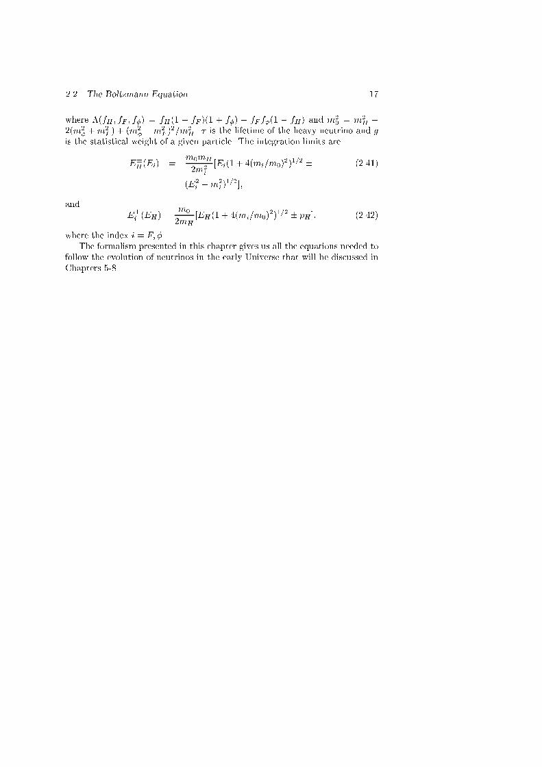
2.2. The Boltzmann Equation 17where �(fH ; fF ; f�) = fH(1 � fF )(1 + f�) � fFf�(1 � fH) and m20 = m2H �2(m2� +m2F ) + (m2� �m2F )2=m2H . � is the lifetime of the heavy neutrino and gis the statistical weight of a given particle. The integration limits areE�H(Ei) = m0mH2m2i [Ei(1 + 4(mi=m0)2)1=2 � (2.41)(E2i �m2i )1=2];and E�i (EH ) = m02mH [EH (1 + 4(mi=m0)2)1=2 � pH ]; (2.42)where the index i = F; �.The formalism presented in this chapter gives us all the equations needed tofollow the evolution of neutrinos in the early Universe that will be discussed inChapters 5-8.

18 Chapter 2. Particle Dynamics in the Expanding Universe

Chapter IIIBasic Big Bang Nucleosynthesis3.1 TheoryAt high temperatures, the baryon content of the Universe is in the form of afree quark-gluon plasma. However, at a temperature of ' 100 MeV this plasmaundergoes a phase transition to a gas of bound quark systems. At �rst, thisplasma consists almost solely of pions, but as the temperature drops, the pionsdisappear and the gas then only consists of neutrons and protons that are \leftover" because of the baryon asymmetry of our Universe. These protons andneutrons are kept in thermodynamic equilibrium by the � reactionsn+ �e $ p+ e�; (3.1)n$ p+ e� + �e; (3.2)n+ e+ $ p+ �e; (3.3)n+ e+ + �e $ p: (3.4)During this era the ratio of protons to neutrons is determined by the Boltzmannfactor np = exp(�(mn �mp)=T ) (3.5)alone. Now, since the rate for these interactions is roughly�� ' G2FT 5 (3.6)and the expansion timescale of the Universe is�H = H�1 =r 38�G�; (3.7)which is proportional to T�2 in a radiation dominated Universe, one arrives atthe relation ����1H ' (T=0:8MeV)3; (3.8)19

20 Chapter 3. Basic Big Bang Nucleosynthesisso that, at a temperature of roughly 1 MeV the average time for n�p conversionwill be longer than the expansion time of the Universe. At this point the con-versions can no longer maintain equilibrium and the neutron to proton fractionfreezes out. From this point on the ratio of neutrons to protons remains con-stant except for the change due to free neutron decays. However, shortly afterthis freeze-out occurs all free neutrons are bound in nuclei thereby preventingfurther neutron decay.Because of the high entropy of the Universe free nucleons are preferred downto very low temperatures, only at T ' 0:2 MeV does deuterium productioncommence. This deuterium is quickly processed into 4He, but at higher A verylittle happens. The reason for this is easy to understand. Because formationof nuclei is suppressed down to very low temperatures the number density isvery low, so that triple reactions are unlikely. Furthermore the Coulomb barrieragainst nuclear reactions is typically very high compared with typical thermalenergies, and there exist no stable A = 5 and A = 8 nuclei. Small amounts of Li,Be and B are produced, but beyond this essentially nothing. In Fig. 3.1 we showthe primary reaction network for primordial nucleosynthesis and in Fig. 3.2 weshow the build-up of light nuclei as the temperature drops.The �nal abundances stemming from BBN depend sensitively on the baryon-to-photon ratio, � � nB � nBn : (3.9)Therefore BBN in principle allows us to determine � if the primordial abun-dances can somehow be determined. Furthermore, the outcome (especially theabundance of 4He) depends on the number of particle species present duringnucleosynthesis. The reason can be seen from the Friedmann equationH2 = 8�G�3 : (3.10)If the number of particle species is increased during nucleosynthesis, this in-creases � and thereby H for given temperature. This again means that ��=His decreased so that the weak interactions decouple earlier than usual. Thus,increasing � during nucleosynthesis has the e�ect of leaving more neutrons tosurvive than normally, meaning that in the end more helium is formed. There-fore one can use Big Bang nucleosynthesis to put limits on novel physics bylimiting the number of particle species that can be present during nucleosyn-thesis. In Fig. 3.3 we show the primordial abundances after nucleosynthesis,both as functions of the baryon-to-photon ratio and of the equivalent number ofneutrinos, N�;eq. This quantity is just a measure of the energy density presentin neutrinos and all other non-electromagnetic interacting particles during nu-cleosynthesis and is de�ned asN�;eq � P ��+X��0 ; (3.11)

3.1. Theory 21

D

n

p3H

4He

7Be

7Li

3He

Figure 3.1: The most important reactions for primordial nucleosynthesis.where �0 indicates a standard massless neutrino species. X indicates novelparticles from physics beyond the standard model that may be present duringnucleosynthesis, such as majorons, axions etc.Finally it should also be mentioned that nucleosynthesis is very sensitiveto the electron neutrino distribution because this enters directly into the �conversion rates through the � process rate integrals of type�n�e!pe = Z f�e(E�e)(1� fe(Ee))jM j2n�e!pe(2�)�5 (3.12)��4(pn + p�e � pp � pe)d3~p�ed3~ped3~pn;where d3~pi = d3pi=(2Ei(2�)3). Thus, one can also put strong limits on physicalprocesses that change the electron neutrino distribution, such as massive orunstable neutrinos. This is a point we shall return to in more detail later.

22 Chapter 3. Basic Big Bang Nucleosynthesis

Figure 3.2: The mass fraction of 4He as well as the number densities of di�erentlight nuclei relative to H as a function of cosmic temperature.3.2 ObservationsA very important but also very di�cult part of this game is the determinationof primordial abundances from observations in the present day Universe. Theobservations are made di�cult by the fact that often the abundances of therelevant elements, such as lithium, are extremely small. However, even moredi�cult is the interpretation of the results. The trouble is that the present dayUniverse has evolved since the Big Bang. Most of the material in the present dayUniverse has been processed through stars and supernovae, changing its chem-ical composition. We will try to give a very brief resum�e of the observationalstatus of the most important Big Bang nucleosynthesis elements.The observation of 4He is relatively easy in the sense that the abundance of4He is large in all astrophysical systems. However, since the primordial heliumabundance is only weakly (logarithmically) dependent on � it is also necessary topin down the primordial fraction to very high precision if one wants to measurethe baryon-to-photon ratio. Since 4He is extremely stable it is very di�cult todestroy and one can assume that it is only produced not destroyed. We alsoknow that no elements with A � 8 are produced in the Big Bang. Therefore

3.2. Observations 23

Figure 3.3: Relic abundances of di�erent nuclei as a function of the baryon-to-photon ratio, �10 � 1010 � nB=n , for di�erent values of N�;eq. The full linesindicate the standard value N� = 3, the dotted ones indicate N�;eq = 2 and thedashed ones N�;eq = 4.

24 Chapter 3. Basic Big Bang Nucleosynthesis

Figure 3.4: Observed abundance of 4He in a number of extragalactic HII regionsas a function of metallicity. The �gure has been reproduced from Ref. [17].if one �nds a system with very low abundance of these heavy elements relativeto the solar values it should indicate that very little processing has taken placeand one may hope that the measured helium abundance in these systems re ectsthe primordial abundance closely. These observations are typically done in largeextragalactic HII regions. In Fig. 3.4 we show a typical example of such a setof observations. The di�culties in pinning down the helium mass fraction,YP � m(4He)=m(H); (3.13)from observations should be obvious looking at the �gure. At present there aretwo papers that re ect the most up to date observational constraints. Unfortu-nately these two papers do not agree with each other on the value found. Firstthere are the results of Olive and Steigman [17] who analyse existing data fromextragalactic HII regions. Doing this they �nd a primordial helium value ofYP � 0:232� 0:003� 0:005; (3.14)where the �rst uncertainty is of purely statistical nature and the second is anestimated systematical uncertainty. The results of Izotov et al. [18] predict amuch higher value for the primordial helium abundanceYP � 0:243� 0:003: (3.15)In Fig. 3.5 we show the results of Izotov et al. corresponding to those shown inFig. 3.4.

3.2. Observations 25

Figure 3.5: The results of Izotov et al. [18] for the abundance of helium. The�gure has been reproduced from Ref. [18].There are two problems in both these results. First of all, the usual way ofgetting the primordial value for helium is to do a linear �t to the observationaldata and interpret the y-axis crossing point as the primordial abundance. Thisassumes that a linear �t makes sense at all, which is by no means obvious. Theother problem is the lack of very metal poor HII regions. Ideally one should�nd just one extremely metal poor object and use the value obtained for heliumin this system as the primordial one. This would eliminate the need for a linear�t using more metal rich objects, but has unfortunately not been possible sofar. Thus, it is not clear what the primordial abundance of helium actually is.Hopefully the coming years will show an increase in the number of metal poorobjects known, so that a more precise value can be found. There are severalongoing projects with this goal.For deuterium the observations used to be done in the solar neighbourhood.However, since D is very fragile and no known process can produce signi�cantamounts of deuterium, these observations give a lower limit to the primordialabundance. The values that have been obtained from such observations aretypically [8] D=H ' 1:6� 10�5: (3.16)In the last few years it has become possible to observe deuterium in quasarabsorption systems at signi�cant redshift. Since these systems have evolved verylittle since the Big Bang one can hope to pin down the primordial deuteriumabundance precisely. Unfortunately the results so far are very controversial.Some of the observations indicate a high deuterium fraction in these clouds

26 Chapter 3. Basic Big Bang Nucleosynthesis[19{21], around D=H ' 2� 10�4: (3.17)However, there are other observations, mainly those by Tytler et al. [22], thatindicate a relatively low deuterium valueD=H ' 3� 10�5; (3.18)which is more consistent with the local value. This low value seems more reli-able since the analysis by Tytler et al. has been extremely careful. Nevertheless,only a few systems have so far been observed and more observations are greatlyneeded. It also appears that there are problems in accomodating a high pri-mordial deuterium value in models of chemical evolution. At present it thusseems very di�cult to draw any conclusions about the primordial value of D.3He has been used together with D in local observations to put an upper limiton the combined abundance of D and 3He. The argument here is that it seemsdi�cult to destroy D without at the same time producing 3He. However, theseresults depend strongly on chemical evolution models and therefore seem nottoo reliable either.For 7Li the situation is also quite muddy. Until the early 80's it was thoughtimpossible to determine the primordial Li abundance from observations becauseLi is both produced and destroyed in astrophysical environments. However in1982 results appeared by Spite and Spite [23], indicating that in a certain groupof very old metal poor halo stars, the 7Li abundance is constant and does notdepend on metallicity. This abundance is then interpreted as the primordialabundance, subject to rather small evolution e�ects compared with normal mainsequence stars. The most recent published determination of the 7Li abundancegives a value of [24]7Li=H = (1:73� 0:05[stat]� 0:2[syst])� 10�10; (3.19)but the systematical uncertainties are, of course, di�cult to estimate since theyinvolve chemical evolution. The trouble is that there may still have been sig-ni�cant depletion even in the plateau stars, so that the value observed there issmaller than the primordial value by some unknown factor. It therefore seemspremature to use 7Li measurements to say anything about the value of �. InFig. 3.6 we show a typical measurement of the 7Li abundance in a group of oldhalo stars. At high masses, almost all Li remains, whereas at lower masses theconvection zone extends deep enough to dissociate Li.In conclusion, there is only one element, namely 4He, whose primordial abun-dance is known to any real precision. However, the trouble is that even herethere is controversy as to the primordial abundance so that a precision deter-mination of � from the observational value of Y is not possible. However, theabundance is still known su�ciently well that one may put rather stringentlimits on new physics. At present, one may fairly certainly conclude that [6]N�;eq � 4 (3.20)

3.2. Observations 27

Figure 3.6: The abundance of 7Li in old halo stars shown as a function ofsurface temperature. The Spite plateau is clearly seen to the left at high surfacetemperatures. The �gure has been reproduced from Ref. [24].so that only the equivalent of one extra neutrino species may be present duringBBN. This bound allows for a fairly large uncertainty in the observational pa-rameters. However, the value of N�;eq favoured is much lower than this, evensomewhat below 3 [8]. The reason for the low value is that the primordial he-lium fraction observed is too low compared to the theoretical predictions. Thismay point to a coming crisis for standard Big Bang nucleosynthesis, so thatnew physics like decaying neutrinos must be invoked to bring consistency. Atthis point, however, it is probably too early to say that there is any real \crisis"for the standard model of primordial nucleosynthesis. Finally, if the primordialvalue of deuterium is ever determined to within a few tens of percent, this willpin down the value of � very accurately because the predicted D abundanceis a very steeply varying function of �. Until then, it is very likely that notmuch progress will be made in determining the baryon-to-photon ratio usingBig Bang nucleosynthesis. Nevertheless, as previously mentioned, there nowseems to be some real hope that it will actually be possible to measure theprimordial deuterium abundance within the foreseeable future.Note that in Chapters 5-8 nucleosynthesis limits will be used several timesto constrain models of neutrinos. However, for historical reasons the limitsused in the di�erent chapters do not necessarily coincide, but rather re ect the

28 Chapter 3. Basic Big Bang Nucleosynthesisobservational status at the time where the speci�c paper was written. Noneof the conclusions change in any signi�cant way by using the most up to dateobservational values.

Chapter IVDirac and Majorana Neutrino InteractionsNeutrinos are an integral part of the standard model of particle physics. Theyare spin-1/2 leptons without electromagnetic charge. As far as we know theyare also massless although there is no fundamental reason why this should be so.In fact there are a number of indications that neutrinos have non-zero masses.These all come from the fact that if neutrinos are massive the di�erent avourstates can mix because these avour states do not necessarily correspond tomass eigenstates.The �rst piece of evidence is from the solar neutrinos [25]. Neutrinos emittedfrom the Sun through the pp reaction can be observed on earth using di�erenttechniques. A common feature of all these experiments is that fewer neutrinosthan expected from standard solar model calculations are seen. It also appearsthat there is no astrophysical solution to this problem in the sense that nosolar models have been able to solve this discrepancy in a satisfactory way. Thetrouble is that the neutrino emission is very sensitive to the central temperatureof the Sun, but if that is changed in order to explain the neutrino ux, othervisible e�ects will occur. The explanation that seems most likely is that theelectron neutrinos emitted from the Sun mix with muon neutrinos which arenot observed on earth, so that this appears as an apparent de�cit in the numberof neutrinos emitted.The second place where evidence for neutrino mass is thought to be seenis the atmospheric neutrinos [26]. These are produced by cosmic rays thatinteract with nuclei in the atmosphere to produce �e, �� and the correspondingantineutrinos. Water Cerenkov detectors like Super-Kamiokande see a strongde�cit in the number of the observed �� � �e ratio compared with the expected ux and this can again be taken as evidence for neutrino oscillations. The lastindication is from the accelerator experiment at the LSND facility [27]. In thiscase evidence for neutrino oscillations is claimed from a �� beam.There has been a large number of terrestrial experiments looking for neutrinomasses. For �e, the endpoint of the tritium decay spectrum is used to look fora non-zero mass, both because the decay is very simple and the Q value is verylow (Q = 14.3 keV) [28]. A small neutrino mass should show up as a de�cit29

30 Chapter 4. Dirac and Majorana Neutrino Interactionsin the electron spectrum near the endpoint energy. However, it turns out thatthere is apparently a small surplus of electrons in this region corresponding toa negative neutrino mass squared. This mystery has been tried resolved forexample by invoking interactions with cosmic background neutrinos, but thise�ect should be too small by many orders of magnitude to explain the observede�ect. So far no good explanation has been produced.For ��, the pion decay �+ ! �+�� has been used to constrain the �� mass.This is done by measuring the decay energy spectrum of the decay productmuons [29].To measure the �� mass, decay of � leptons is used. The speci�c decay is� ! 5���0�� and the measured quantities are the invariant mass as well as theenergy of the hadronic decay products [30]. Altogether, the present upper masslimits are m�e � 15eV[7] (4.1)m�� � 170keV[29] (4.2)m�� � 24MeV[30] (4.3)4.1 De�nition and Properties of Neutrino Fields 1Only two physical neutrino states are known, the left handed neutrino andthe right handed anti neutrino. The other fermions are known to be Diracparticles, having both left and right handed particles and antiparticles, butpossibly neutrinos are describable in a theory containing only two components.We distinguish between these two fundamental ways of building the theory ofneutrinos, the four component Dirac neutrino and the two component Majorananeutrino. Let us start out from the de�nition of the neutrino �elds. The Dirac�eld is de�ned in the same way as for the other fermions D = Z d3p2E(2�)3 Xs hfsuse�ip�x + fysvseip�xi ; (4.4)where u and v are the plane wave solutions to the Dirac equation for positiveand negative energy respectively( �p� �m)us(p) = 0 (4.5)(� �p� �m)vs(p) = 0: (4.6)fs is the particle annihilation operator and fys is the creation operator for an-tiparticles fs(p)jp; si = j0i (4.7)fys(p)j0i = jp; si: (4.8)1This section borrows heavily from Ref. [31].

4.1. De�nition and Properties of Neutrino Fields 31We use the standard normalisation of the Dirac spinorsuys(p)us0(p) = 2E�ss0 (4.9)vys(p)vs0(p) = 2E�ss0 (4.10)vys(p)us0(p) = 0 (4.11)The Majorana �eld, on the other hand, is de�ned using only two components D = Z d3p2E(2�)3 Xs �fsuse�ip�x + �fys vseip�x� ; (4.12)where � is a phase called the creation phase factor. It can be chosen at will, butit is not always advantageous to choose it as � = 1. For this reason it is usuallykept as a free parameter to de�ne. The obvious di�erence between Dirac andMajorana �elds is that the Majorana �eld is de�ned by only two components.Essentially this must also mean that a Majorana particle is its own antiparticle.To show this we need a few de�nitions. We start with a spinor �eld, (x).Under a Lorentz tranformationx0� = x� + !�� x� ; (4.13)the spinor �eld transforms as [32] 0(x0) = exp� i4���!��� (x); (4.14)where ��� = i2[ �; � ]: (4.15)To de�ne a conjugate �eld that transforms in this way it is not enough to use �. The reason is that � does not transform in the same way as underLorentz transformations, instead it obeys the transformation law �0(x0) = exp�� i4����!��� �; (4.16)which is not the same as Eq. (4.14). We de�ne the conjugate �eld as � C 0 0 �; (4.17)where, by �, we mean the column vector � = 0BBB@ y1 y2 y3 y4 1CCCA :

32 Chapter 4. Dirac and Majorana Neutrino InteractionsC 0 is some operator which will, in a moment, be identi�ed with the chargeconjugation operator. For consistency C 0 must obey the condition�C 0 0���� = ���C 0 0: (4.18)So far we have not discussed things in a speci�c representation basis, but wenow shift to the Dirac representation in which 0 = � I 00 �I � i = � 0 �i��i 0 � ; (4.19)where �i are the Pauli matrices. In this basis we can choose C 0 = i 2 0 so thatit obeys the condition, Eq. (4.18). Under the operation of charge conjugationany fermion �eld transforms asC C�1 = ��CC 0 �; (4.20)where �C is a phase factor. Let us now check the e�ect of using our operatorC on the Dirac �eld to see that we can indeed make the identi�cation C 0 = C.We do this by assuming C 0 = C and from there show that this identi�cationmakes sense. The right hand side of Eq. (4.20) gives��CC 0 � = ��Ci 2 � (4.21)and, if we use the plane wave expansion,��CC 0 � = ��C Z d3p2E(2�)3 Xs �fsuseip�x + fys vse�ip�x� ; (4.22)since 2u� = v (4.23) 2v� = u: (4.24)On the other hand, the left hand side givesC DC�1 = Z d3p2E(2�)3 Xs hCfsC�1useip�x + CfysC�1vse�ip�xi : (4.25)Putting the two equations together we obtain the following relations for thecreation and annihilation operatorsCfsC�1 = ��Cfs (4.26)CfysC�1 = �Cfys: (4.27)The e�ect of C on a state jp; si is thenCjp; si = �C jp; si: (4.28)

4.2. Neutrino Weak Interactions 33Altogether then, this means that the e�ect of C 0 is to change a physical stateinto a corresponding state for the antiparticle, justifying our identi�cation ofthe operator C 0 with the charge conjugation operator C.Finally, we are now ready to apply the same procedure to the Majorana�eld. Here, one �nds that C MC�1 = (�C�)� M ; (4.29)where we have used our plane wave de�nition of the Majorana �eld, Eq. (4.12).The Majorana �eld is thus, apart from a phase factor, invariant under chargeconjugation. In exactly the same way as for the Dirac �eld one may show thatthe following relations hold for the creation and annihilation operators,CfsC�1 = �C�fs (4.30)CfysC�1 = �C�f ys : (4.31)If we now apply this to a free Majorana state we getCjp; si = �C�jp; si; (4.32)so we see that a free Majorana state is an eigenstate of charge conjugation.Similar relations apply for CP and CPT , speci�cally for CPT one �nds therelation CPT jp; si = �CPT�(�1)s�1=2jp;�si; (4.33)where �CPT is again a phase. This indeed means that the left and right handedstates are particle and anti particle in the usual sense, since application of theCPT operator on a left handed Majorana state turns it into a right handedstate with the same momentum.4.2 Neutrino Weak InteractionsLet us now look at the interactions of neutrinos to see the di�erence betweenDirac and Majorana neutrinos. At su�ciently low energies, neutrinos interactvia a current-current interaction because of the large masses of the gauge bosons(W�; Z0) so that the weak hamiltonian density to lowest order in the couplingconstant has the form Hweak = GFp2j�(x)j�(x): (4.34)This interaction is described by the standard V �A theory. In the present workwe are only interested in purely leptonic interactions, meaning that the termswe are interested in are the leptonic charged currentjCC� = Xe;�;� i(x) �(1� 5) �i (x); (4.35)

34 Chapter 4. Dirac and Majorana Neutrino Interactionsthe charged fermion neutral currentjNC� = Xe;�;� i(x) �(gV � gA 5) i(x); (4.36)and the neutrino neutral currentjNC� = Xe;�;� �i(x) �(1� 5) �i(x): (4.37)gV and gA are the charged fermion vector and axial vector neutral current cou-plings respectively. They are given in terms of the Weinberg angle, sin2�W =0:2325� 0:0008, as CV = �12 + 2 sin2�W (4.38)CA = �12 : (4.39)The S matrix is then given byS = 1� i Z d4xHweak; (4.40)and from this all matrix elements are calculable.There is no a priori reason why Dirac and Majorana neutrinos should behavethe same under these interactions. However, because of the left handedness ofthe weak interactions it turns out that interactions that are di�erent for Diracand Majorana neutrinos always scale as some power of neutrino mass. Thismeans that for massless neutrinos, Dirac and Majorana neutrinos are indistin-guishable. However, if neutrinos are massive Dirac and Majorana neutrinosbehave di�erently. For example there is no conserved lepton number if neutri-nos are Majorana particles because neutrinos can ip their spin direction andthereby violate lepton number by two units. If we look at Majorana neutri-nos, it is straightforward to show that they possess no neutral current vectorinteractions. This is true because of the relation c � c = � � ; (4.41)which holds for any fermion �eld. However, since the majorana �eld is invariantunder C up to a phase this implies that M � M = � M � M = 0 (4.42)Furthermore, there is the di�erence that the Majorana �eld M can both createand destroy neutrino states as opposed to the Dirac �eld M that only containsthe annihilation operator for neutrinos.One should perhaps think that this di�erence leads to observable e�ects evenfor massless neutrinos. However, for massless neutrinos there is no detectable

4.2. Neutrino Weak Interactions 35di�erence between Majorana and Dirac neutrinos. Neutrinos are either createdin pairs via neutral current reactions or as a single neutrino or anti-neutrino viacharged current reactions. In the case of neutral current reactions, the neutrinopair is not born with de�nite helicity. This has nothing to do with lack of vectorcurrent interactions but is rather an e�ect of wave packet superposition, andis independent of whether neutrinos are of Dirac or Majorana type. We nowlook at the detection of neutrinos created via neutral current reactions. Sincethe charged current is still left handed even for Majorana neutrinos, if theseneutrinos are detected via charged current reactions, only the left handed com-ponent will interact and one therefore detects either particles or antiparticles,but not both. The left handedness of the charged current thus \reintroduces"the vector current for Majorana neutrinos, making them behave as Dirac parti-cles. This means that there is absolutely no detectable di�erence between Diracand Majorana neutrinos in this case. If they are detected via neutral currentreactions, there is no way to measure their helicity anyway and, again, there isno detectable di�erence. Next, we look at neutrinos created via charged currentreactions. These are born with de�nite helicity and, even if detected by neu-tral current reactions, still behave as if they do possess vector neutral currentinteractions because of the de�nite helicity of their initial state.Also, of course, the two super uous states for Dirac neutrinos, the righthanded neutrino and the left handed anti neutrino are completely sterile ifneutrinos are massless because of the (1� 5) factor in the weak current. Thusthey are not relevant for the massless standard model neutrinos.This discussion about the possible di�erences between Dirac and Majorananeutrinos have given rise to some discussion recently [33]. It was claimed thatthe measurement of the �� � e vector neutral current coupling constant by theCHARM II collaboration [35] givingCV = �0:035� 0:017; (4.43)excludes the neutrino as being a Majorana particle [34]. In light of the discussionabove this cannot be the case of course, since the muon neutrinos observed byCHARM II are produced by the charged current decays of charged kaons andpions [35] and therefore they are born with de�nite helicity. Therefore theyare observed as having vector current interactions even if they are Majoranaparticles.For massive neutrinos, the situation is much more complex. Here, all thefour states for Dirac neutrinos are active so that Majorana and Dirac neutrinosbehave di�erently. Also their weak interaction cross sections are di�erent. Inthe early Universe it is therefore important to distinguish between Dirac andMajorana neutrinos if their mass su�ciently large. For Dirac neutrinos, if themass is below roughly 0.2-0.3 MeV the two \sterile" states decouple prior to theQCD phase transition so that their number density is diluted by a large factorbecause of the entropy release from the phase transition. In this case they do notcontribute to the cosmic energy density during nucleosynthesis. Also, the massis then su�ciently low that the Dirac and Majorana annihilation cross sections

36 Chapter 4. Dirac and Majorana Neutrino Interactionsare practically identical until long after they have decoupled. Therefore, atthese low masses the two types are again indistinguishable. For higher massesone needs to do a full calculation for all four states of Dirac neutrinos, andone can expect that Dirac and Majorana neutrinos have a completely di�erentimpact on nucleosynthesis. In Fig. 4.1 we show the relic number density ofmassive neutrinos during nucleosynthesis times neutrino mass. This is a goodmeasure of the energy density contributed during BBN by a massive neutrino,either Majorana or Dirac. It is seen that the Dirac neutrino in most of themass region contributes much more than the corresponding Majorana neutrinobecause it has four interacting states. For large masses, however, the Majoranaannihilation cross section is smaller than the Dirac one so that the Majorananeutrinos actually contribute more to the cosmic energy density. The crosssection for annihilation into massless �nal states is for non-relativistic neutrinosgiven by h�jvjiDirac = G2Fm22� Xi (C2V;i + C2A;i) (4.44)h�jvjiMajorana = G2Fm22� Xi 8�2(C2V;i + C2A;i)=3 (4.45)where � is the relative velocity of the incoming particles. This shows the strongdi�erence between Dirac and Majorana neutrinos in the non-relativistic limit.The cross section is velocity dependent for Majorana neutrinos whereas it is notfor Dirac neutrinos. As the neutrino kinetic energy becomes smaller and smallerrelative to the mass the Dirac cross section is increased relative to the Majoranaone, and this is the reason why very heavy Majorana neutrinos contribute morethan Dirac neutrinos at high mass.In the remainder of this work we shall only be concerned with Majoranatype neutrinos. The good thing about these is that one need only consider thetwo usual states. Furthermore, since there is very little lepton asymmetry in theearly Universe, Majorana neutrinos e�ectively behave as one single unpolarisedparticle species. Interaction cross sections and the like are therefore relativelyeasy to calculate in this case.4.3 Mixed NeutrinosIf neutrinos are massive they may in principle mix. The reason is that thestates produced by the weak interaction are not necessarily mass eigenstates.In general there exists a unitary transformation between the weak interaction( avour) eigenstates and the mass eigenstatesj�f i = U j�mi; (4.46)where U is a unitary matrix. Therefore, if neutrinos have mass, the freelypropagating neutrinos may oscillate between di�erent avours. This is very

4.4. Decaying Neutrinos 37

Figure 4.1: The number relic number density times mass of a massive neutrino,de�ned in units of the number density of a massless neutrino species rm �n=n(m = 0)�m. The full line is for Dirac neutrinos and the dotted for Majorananeutrinos. The discontinuity at m ' 0:3 MeV for Dirac neutrinos indicate thatabove this mass all four states are in equilibrium below the QCD phase transitiontemperature. The �gure has been reprinted from Ref. [36].important for our understanding for example of the solar neutrino problem.They are of course potentially very interesting for BBN as well. However inthe present work we shall not deal with neutrino oscillations at all. We shallbe looking at mixed neutrinos in the context of neutrino decays but neglect thepossible oscillations between avours. This particular area is, however, de�nitelyworthy of further study.4.4 Decaying NeutrinosIn the standard model neutrinos do not have mass and therefore they are ab-solutely stable. However, once a mass term is introduced this is no longer so.Also, if the mass is larger than roughly 100 eV for any neutrino it must beunstable with a lifetime shorter than the Hubble expansion time in order not tooverclose the Universe [36], but there are many possible decay modes for such

38 Chapter 4. Dirac and Majorana Neutrino Interactionsneutrinos. For example within the standard model the decay �i ! �ee+e� ispossible at tree level provided that m�i � 2me and that the mixing amplitudebetween the two neutrino avours is di�erent from zero. Another possibility isthe neutrino radiative decay �i ! �j which is mediated by interactions at looplevel. If there exists a avour violating neutral current there is also the decayto a three neutrino �nal state �i ! �j�k�k. Further beyond the standard modelthere are decays like �i ! �j� where � is some new particle like the majoron.There is a large number of models for physics beyond the standard modelthat predict di�erent neutrino lifetimes to the di�erent decay modes. Our ap-proach will be to discuss the experimental limits to the di�erent decay modes,not so much to go into speci�c physical models of neutrino decays.We start out with the simplest possible decay, namely �i ! �ee+e�. Thisdecay mode is relatively easy to constrain because the decay products interactelectromagnetically. If we restrict ourselves to the three known neutrino gener-ations only the � neutrino mass is not required to be below the threshold forthis decay mode. Within the standard model the decay lifetime is given by [11]��1 = 3:5� 10�5jUe� j2m5MeV�(m2�� =m2e) s�1; (4.47)where jUe� j is the mixing between electron and tau neutrino and � is a phasespace factor dependent on the tau neutrino mass�(q) = (1� 4q)1=2(1� 14q � 2q2 � 12q3) + (4.48)24q2(1� q2) ln�1 + (1� 4q)1=21� (1� 4q)1=2� :Strong limits on this decay come from SN1987A because of the very intensetau neutrino production from this source. Furthermore a tau neutrino with massin the relevant region should decay su�ciently early that the decay products donot overclose the Universe. These limits have been summarised by Ra�elt [11]and e�ectively this decay mode has been excluded by existing data. In Fig. 4.2we show the excluded regions for this decay from both SN1987A, cosmologicaland other constraints.Next we turn to the radiative decay of heavy neutrinos, �i ! �j . Unlessthe neutrino possesses a small electromagnetic charge the radiative decay ofneutrinos proceed via loop graphs. Therefore the decay lifetime is exceedinglylong in all viable models that have so far been constructed. From an argumentusing the cooling of red giant stars it is possible to constrain severely the chargeof neutrinos. The reason is that if neutrinos do possess charge they couple tothe photon at tree level and therefore plasma excitations can produce neutrinopairs at a much higher rate than in the standard model. This leads to a veryfast cooling of stars, in con ict with observations. From this argument anupper bound of q� � 2� 10�14e on the neutrino charge can be derived [11]. Inconclusion it does not seem possible to construct models that predict neutrinoradiative decay lifetimes shorter than the lifetime of the Universe.

4.4. Decaying Neutrinos 39

Figure 4.2: Exclusion plot for the decay �� ! �ee+e�. The excluded regionindicated by the arrow to the right is from limits to the galactic positron anni-hilation line ux. This �gure has been reproduced from Ref. [11].The radiative decay is relatively easy to constrain experimentally becauseof the emitted photon that interacts electromagnetically. In the most generalcase the decay rate can be expressed in terms of an e�ective electromagnetictransition moment, �� , as ��1 = �2�m38� : (4.49)Bounds can be placed on this transition moment from observations of SN1987A.These come from the gamma ray observations made by the solar maximummission satellite and have been discussed in great detail by for example Ra�elt[11].However, the most interesting limits come from cosmological considerations,especially from observations of the cosmic microwave background and the dif-fuse photon background. These mainly concern neutrinos with long lifetime,but since it is probably impossible to construct viable physical models that pre-dict short neutrino lifetimes to radiative decay this is exactly the region we areinterested in constraining. The relevant limits have been compiled by for exam-ple Kolb and Turner [36]. Fig. 4.3 shows the excluded regions reproduced from

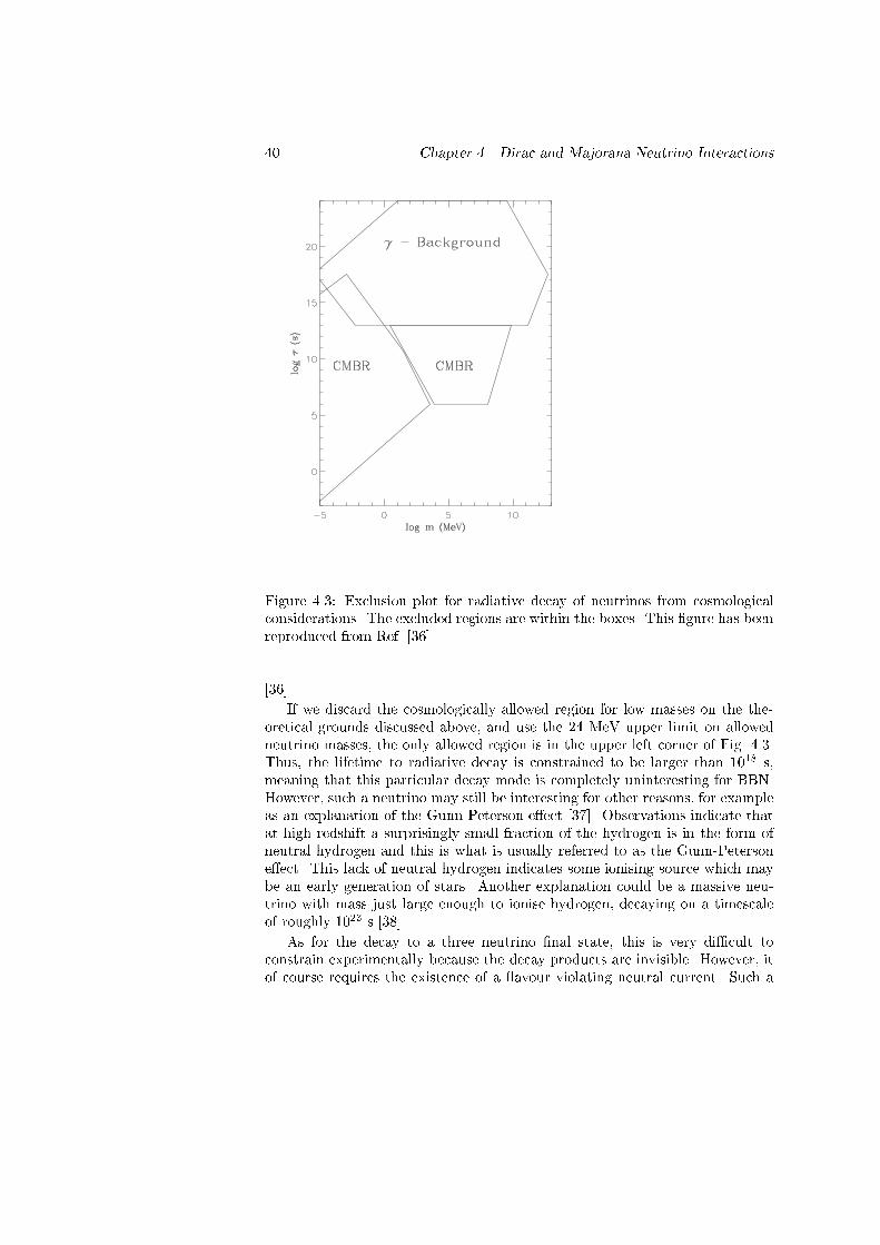
40 Chapter 4. Dirac and Majorana Neutrino Interactions

Figure 4.3: Exclusion plot for radiative decay of neutrinos from cosmologicalconsiderations. The excluded regions are within the boxes. This �gure has beenreproduced from Ref. [36].[36].If we discard the cosmologically allowed region for low masses on the the-oretical grounds discussed above, and use the 24 MeV upper limit on allowedneutrino masses, the only allowed region is in the upper left corner of Fig. 4.3.Thus, the lifetime to radiative decay is constrained to be larger than 1018 s,meaning that this particular decay mode is completely uninteresting for BBN.However, such a neutrino may still be interesting for other reasons, for exampleas an explanation of the Gunn-Peterson e�ect [37]. Observations indicate thatat high redshift a surprisingly small fraction of the hydrogen is in the form ofneutral hydrogen and this is what is usually referred to as the Gunn-Petersone�ect. This lack of neutral hydrogen indicates some ionising source which maybe an early generation of stars. Another explanation could be a massive neu-trino with mass just large enough to ionise hydrogen, decaying on a timescaleof roughly 1023 s [38].As for the decay to a three neutrino �nal state, this is very di�cult toconstrain experimentally because the decay products are invisible. However, itof course requires the existence of a avour violating neutral current. Such a

4.4. Decaying Neutrinos 41current would also give rise to processes like �� ! e�e+e� which are stronglyconstrained experimentally [39]. The best constraints on the decay itself comefrom BBN considerations, the most recent calculation being that of Dodelson,Gyuk and Turner [40]. In general neutrinos with mass in the MeV region areexcluded if their lifetime is too long. For very light neutrinos (m� MeV) BBNdoes not in general exclude this type of decay because it only becomes importantafter BBN has already taken place.Finally, in the present work we shall only deal with neutrino decays of thetype �i ! �j�. Exactly as for the previous decay mode to three neutrinosthis decay mode is of course not easy to constrain since the decay products areinvisible. For the class of models called majoron models the above coupling to� also leads to processes like neutrinoless double beta decay and from this someconstraints can be put on the possible decay strength. However, these are veryweak and at the moment the best constraints come from the BBN considerationsdiscussed in more detail in Chapters 7 and 8.

42 Chapter 4. Dirac and Majorana Neutrino Interactions

Chapter VNeutrino decoupling in the Standard ModelEssentially all of this chapter has appeared as the paper Neutrino Decouplingin the Early Universe, Phys. Rev. D 52, 1764 (1995).Nonequilibrium thermodynamics is fundamental to the understanding of theearly Universe. There are many examples of this, the quark-hadron phase tran-sition, the electroweak phase transition, in ation etc. Another example is thedecoupling of neutrinos from the electromagnetic plasma at a temperature ofa few MeV. The normal assumption [36] is that neutrinos decouple completelybefore the temperature approaches the mass of the electron. When the temper-ature gets below the electron rest mass, the electrons and positrons annihilateand pump energy and entropy into other particles. But since the neutrinos aredecoupled they do not share in this transfer. Their �nal distribution is there-fore still described by an equilibrium distribution, but with a lower temperaturethan the photon temperature, T� = (4=11)1=3T .However, this is not the complete story. The fact that the decoupling tem-perature is of the same order as the electron mass means that neutrinos must,to some degree, share the entropy transfer. This phenomenon is known as neu-trino heating. Because it has consequences for Big Bang Nucleosynthesis, it hasbeen investigated many times in the literature [41{45]. All of these investiga-tions have found that the change in neutrino energy density is of the order 1%, relative to the standard case where total decoupling is assumed. This is toosmall a change to have any noticeable e�ect on nucleosynthesis.One possible problem is, however, that they all assume that Boltzmannstatistics is a good approximation for all particle distribution functions. Thismeans that e�ects that depend on quantum statistics, such as Pauli blockingof �nal states, are neglected. Furthermore they also neglect the electron massin the weak interaction matrix elements. This approximation is valid as longas the temperature is high, but possibly not when it is comparable to, or lowerthan, the electron mass.Since the neutrino distributions are important both for nucleosynthesis and43

44 Chapter 5. Neutrino decoupling in the Standard Modelstructure formation models, it is of considerable interest to see if neutrino heat-ing has any consequences for either.5.1 Fundamental EquationsAs explained in Chapter 2, the equation necessary to describe all the di�er-ent particle interactions is the Boltzmann equation. Since we are looking atstandard weak interactions at low energy, all processes can be calculated usingsimple V-A theory as explained in Chapter 4. To �rst order in the weak couplingconstant, GF , all interactions are two-particle scatterings and annihilations andthe matrix elements therefore are all of the same type. As an example we showthe matrix element for the neutral current process �i�j ! �i�j ,M = GFp2u�i � 1� 52 u�iu�j � 1� 52 u�j : (5.1)All the possible reactions and their corresponding matrix elements have beensummarised in Tables 5.1 and 5.2. Higher order corrections to these matrixelements as well as electromagnetic corrections from plasma processes are ne-glected. The collision integral on the right hand side of the Boltzmann equationthen has the form given in Eq. (2.29). Assuming standard weak interactions asdescribed in Chapter 4, it is possible to analytically integrate this 9 dimensionalintegral down to two dimensions (Appendix B). This makes the integral mucheasier to evaluate numerically.The problem now is to evaluate R(t). This can basically be done in two ways,using either entropy or energy conservation (see Chapter 2). As explained inRef. [46], the end result is almost the same for massless neutrinos.5.2 Numerical ResultsWe have solved the coupled Boltzmann equations together with the entropyconservation equation to obtain numerical results. The equations were solvednumerically by using a grid of 35 points in momentum space and a Runge-Kuttaintegrator to evolve the relevant quantities forward in time. To compare withprevious results, we have solved for several di�erent cases: 1. me 6= 0 andFD statistics; 2. me = 0 and FD statistics; 3. me 6= 0 and MB statistics; 4.me = 0 and MB statistics. In all cases we assume zero chemical potentials forthe particles involved at the initial temperature. Case 4 is the approximationused in previous studies. Case 1 is the correct approach.For each of these scenarios we have calculated the energy density deviation,de�ned as ���=�� = (�� � ��0)=�� , as a function of the photon temperature T .��0 is the energy density of a neutrino species that has decoupled long beforee� annihilation.For electron neutrinos, the result is shown in Fig. 5.1, whereas Fig. 5.2 showsthe result for muon and tau neutrinos. In the limit of MB statistics and zero

5.2. Numerical Results 45Table 5.1: Possible electron neutrino processes and the corresponding matrixelements for massless Dirac neutrinos. 1 is de�ned equal to the particle forwhich we calculate Ccoll. 2 is the other incoming particle. 3 is de�ned as eitherparticle 1 going out (scattering) or the outgoing lepton (annihilation). 4 isde�ned as either particle 2 going out (scattering) or the outgoing antilepton(annihilation). We have introduced the quantities CV = 12 + 2 sin2 �W andCA = 12 , where sin2 �W � 0:23. pi is the four-momentum of particle i.Process S jM j2�e + �e ! �e + �e 128G2F (p1 � p4)(p2 � p3)�e + �e ! �e + �e 32G2F (p1 � p2)(p3 � p4)�e + �i ! �e + �i 32G2F (p1 � p2)(p3 � p4)�e + �i ! �e + �i 32G2F (p1 � p4)(p2 � p3)�e + e� ! �e + e� 32G2F [(CA + CV )2(p1 � p2)(p3 � p4)+(CA � CV )2(p1 � p4)(p2 � p3)�(C2V � C2A)m2e(p1 � p3)]�e + e+ ! �e + e+ 32G2F [(CA + CV )2(p1 � p4)(p2 � p3)+(CA � CV )2(p1 � p2)(p3 � p4)�(C2V � C2A)m2e(p1 � p3)]�e + �e ! e� + e+ 32G2F [(CA + CV )2(p1 � p4)(p2 � p3)+(CA � CV )2(p1 � p3)(p2 � p4)+(C2V � C2A)m2e(p1 � p2)]�e + �e ! �i + �i 32G2F (p1 � p4)(p2 � p3)electron mass (case 4), we reproduce the results of Ref. [41] to within 10-15%. This is quite reassuring, as we use a completely di�erent procedure forsolving the Boltzmann equations. Dodelson and Turner [41] used a �rst orderperturbation expansion, f�i(p; t) = f0(p) + ��i(p; t); (5.2)and T = T�(1 + �(t)): (5.3)They then solved the perturbation equations for ��i(p; t) and �(t).Using the correct quantum statistics and non-zero electron mass (case 1),the �nal result for the deviation in energy density is roughly0:83% for �e0:41% for ��; �� (5.4)Generally, it is seen that the deviation is smaller if Fermi statistics is used. Thisis because the Pauli blocking factors in the collision integral, Eq. (2.30), dampenthe interactions. Furthermore using the correct electron mass also lessens thedeviation because the structure of the matrix elements changes.

46 Chapter 5. Neutrino decoupling in the Standard ModelTable 5.2: Possible �; � neutrino processes and matrix elements. The de�nitionof particle numbers is the same as in table 5.1.Process S jM j2�i + �i ! �i + �i 128G2F (p1 � p4)(p2 � p3)�i + �j ! �i + �j 32G2F (p1 � p4)(p2 � p3)�i + �i ! �i + �i 32G2F (p1 � p2)(p3 � p4)�i + �j ! �i + �j 32G2F (p1 � p2)(p3 � p4)�i + �e ! �i + �e 32G2F (p1 � p4)(p2 � p3)�i + �e ! �i + �e 32G2F (p1 � p2)(p3 � p4)�i + e� ! �i + e� 32G2F [(CV + CA � 2)2(p1 � p2)(p3 � p4)+(CA � CV )2(p1 � p4)(p2 � p3)�[(CV � 1)2 � (CA � 1)2]m2e(p1 � p3)]�i + e+ ! �i + e+ 32G2F [(CV + CA � 2)2(p1 � p4)(p2 � p3)+(CA � CV )2(p1 � p2)(p3 � p4)�[(CV � 1)2 � (CA � 1)2]m2e(p1 � p3)]�i + �i ! e� + e+ 32G2F [(CV + CA � 2)2(p1 � p4)(p2 � p3)+(CA � CV )2(p1 � p3)(p2 � p4)+[(CV � 1)2 � (CA � 1)2]m2e(p1 � p2)]�i + �i ! �e + �e 32G2F (p1 � p4)(p2 � p3)�i + �i ! �j + �j 32G2F (p1 � p4)(p2 � p3)Apart from the changes in energy density, the shape of the distributionfunctions are changed from their equilibrium form. We parametrise this changeby using an e�ective temperature for the neutrino distributions, de�ned as [41]TFDe� (p) � pln(1=f(p)� 1) (5.5)for Fermi-Dirac statistics and TMBe� (p) � �pln f(p) (5.6)for Maxwell-Boltzmann statistics.Fig. 5.3 shows the e�ective temperature using Fermi statistics, both withand without electron mass incorporated. Note that the e�ective temperatureof a completely decoupled neutrino is T� ' 0:714T . Fig. 5.4 shows the same,but using Boltzmann statistics. Notice the general o�set in e�ective tempera-ture compared to Fig. 5.3. This is because the �nal e�ective temperature of adecoupled neutrino is T� ' 0:693T if Boltzmann statistics is used (see Chapter2). We see that, regardless of the statistics used, the e�ective temperature riseswith momentum for medium and high momentum states. As noted in Refs.[41, 42], this is not surprising, because the weak cross sections are much largerfor large momenta. The shape of the e�ective temperature curve is the same in

5.3. Discussion and Conclusions 47

Figure 5.1: The evolution of ���=�� for electron neutrinos. The solid curvecorresponds to case 1, the dashed to case 2, the dotted to case 3, and thedot-dashed to case 4.all four cases, but the actual numerical values are slightly di�erent, being higherif the electron mass is neglected in Ccoll[f ]. This e�ect re ects that the neutrinoenergy density is slightly higher for massless electrons, as seen in Fig. 5.1.5.3 Discussion and ConclusionsWe have calculated the decoupling of massless neutrinos in the early Universeby solving the Boltzmann equations. Our method di�ers from previous studiesin that it makes no approximations for the neutrino distribution functions andthe weak interaction matrix elements. Although our results do not deviatedramatically from these previous calculations, we show that the inclusion of FDstatistics and non-zero electron mass reduce the e�ect of neutrino heating onthe relativistic neutrino energy density by almost 50% for �e, compared to theresults of Dodelson & Turner [41].We �nd that the neutrino distribution after decoupling is non-thermal atthe 1% level. This is also in relatively good agreement with previous results[41, 42]. The e�ective temperature grows with momentum for medium and large

48 Chapter 5. Neutrino decoupling in the Standard Model

Figure 5.2: The evolution of ���=�� for muon and tau neutrinos. The curvelabels are as in Fig. 1.momenta, because of the momentum dependence of the weak interactions.The slight heating of neutrinos relative to the standard scenario has con-sequences for Big Bang nucleosynthesis. We have changed the nucleosynthesiscode of Kawano [47] to include the e�ect of neutrino heating. As discussed inRef. [48], there are several e�ects that combine to change the nucleosynthesisscenario. First of all, the energy density in neutrinos is changed. However, thishas the consequence of lowering the energy density in photons and e�, becauseof energy conservation. The result is, if we use FD statistics and non-zero elec-tron mass, that the photon temperature goes up because of e� annihilations bya factor of 1.3998 instead of the usual 1.4010 (a change of �0:09%). Further-more, the weak rates are changed, because of the di�erent abundances of e� and�e. With the relevant changes to the code, we obtain a change in the primordial4He abundance, YP , of �Y = +1:0�10�4. This is in good agreement with Ref.[48]. They calculate a change of +1:5� 10�4, but with a 50% larger neutrinoheating. Other authors have found similar values [42, 43]. A change in 4Heabundance of = +1:0 � 10�4 is much below current observational accuracies.The systematic uncertainty in the primordial 4He abundance is estimated to beas large as �Ysys = +0:016=� 0:012 [49], or more than a factor of 100 larger

5.3. Discussion and Conclusions 49

Figure 5.3: The e�ective neutrino temperature after complete e� annihilation,using FD statistics. The solid line is for �e and case 1, the dashed is for ��;�also case 1. The dotted is for �e and case 2, the dot-dashed for ��;� and case 2.than the change induced by neutrino heating.Another consequence of neutrino heating is that it increases the numberdensity of neutrinos. If one of the neutrino species has a mass, it will thereforecontribute slightly more than usually expected to , the cosmological densityparameter. In general, it is possible to put a mass limit on a light neutrino thatis completely decoupled long before e� annihilation [50]. The mass density ofsuch a species today is �� = n�m� : (5.7)Expressing this in terms of the photon density, n = 2�(3)T 3 =�2, one gets�� = m� n�n �(3) 2�2 T 3 ; (5.8)where �(x) is the Riemann zeta-function. If the neutrinos decouple long beforee� annihilation, this can be translated into the normal textbook relation�h2 = g�2 m�93:03eV ; (5.9)

50 Chapter 5. Neutrino decoupling in the Standard Model

Figure 5.4: The e�ective neutrino temperature after complete e� annihilation,using MB statistics. The solid line is for �e and case 3, the dashed is for ��;�also case 3. The dotted is for �e and case 4, the dot-dashed for ��;� and case 4.using a present photon temperature of 2.736 K. h is the dimensionless Hubbleconstant, and g� = 2 for one avour of neutrino and antineutrino. Since obser-vations demand that �h2 � 1 [36], we have a mass limit on any given lightneutrino. Because of neutrino heating, this limit is changed by a small amount.Using FD statistics and non-zero me� , the �nal number density of neutrinosafter decoupling deviates from the standard case by �n�=n� � 0:52% for �e and�n�=n� � 0:25% for ��;� . For electron neutrinos this changes Eq. (5.9) to�eh2 = g�e2 m�e92:55eV ; (5.10)whereas for muon or tau neutrinos we �nd��;�h2 = g��;�2 m��;�92:80eV : (5.11)As this is a very small change to the standard value, neutrino heating does notalter the usual conclusion that electron neutrinos can not contribute more thanabout 0.5 (using the current experimental upper limit to its mass, m�e � 15 eV[7]) to , whereas muon and tau neutrinos can.

5.3. Discussion and Conclusions 51The main conclusion is that it is safe to ignore neutrino heating when doingnucleosynthesis and structure formation calculations. However, one should notethat neutrino heating is a non-negligible e�ect if one wants to construct a highprecision BBN code. It should also be noted that since this work was performednew results by Dolgov et al. [51] have appeared. They use the same basicapproach as ours but with much higher numerical precision and their resultscon�rm ours very nicely. Their results for the neutrino energy density changeare ���e=��e = 0:9% and ����=��� = 0:4% compared to our result of ���e=��e =0:83% and ����=��� = 0:41%. They �nd a resulting increase in the primordialHe production of �Y = +1:4� 10�4 which is somewhat larger than our result,�Y = +1:0 � 10�4. However, their implementation into the nucleosynthesiscode di�ers from ours to some extent which may explain this small di�erence.

52 Chapter 5. Neutrino decoupling in the Standard Model

Chapter VIMassive Stable Neutrinos in BBNEssentially all of this chapter has appeared as the paper Nucleosynthesis andthe Mass of the Tau-Neutrino Revisited, Phys. Rev. D 54, 7894 (1996).The possibility of heavy � neutrinos in the MeV region has been investigatedmany times in the literature, primarily because such a neutrino could have veryinteresting consequences for both cosmology and supernovae [52]. In Chapter 4we discussed the mass limits on the di�erent neutrino species. The best currentexperimental limit to the � neutrino mass comes from the ALEPH collabora-tion [30], and is m�� � 24 MeV with 95 % CL. Primordial nucleosynthesis putsstringent limits on the mass and lifetime of the � neutrino [12, 40, 53{60]. Thebounds are most stringent for neutrinos in the MeV region because their massis comparable to the weak decoupling temperature. This can be seen from thefollowing argument. As long as massive neutrinos are kept in weak equilib-rium with the relativistic species their number density is that of a species inthermodynamic equilibrium. That is, if the mass is much smaller than the tem-perature, the number density is roughly equivalent to that of a massless species,whereas if the mass is much larger than the temperature, the number density isexponentially suppressed nnmassless / exp(�m=T ): (6.1)As soon as the massive neutrinos decouple their number density stays constantrelative to that of a massless species. However, their energy density starts grow-ing as the temperature drops because the energy density becomes dominated bythe rest mass term. In this case the energy density scales as�NR / mT 3; (6.2)whereas for relativistic species the energy density scales as�R / T 4; (6.3)53

54 Chapter 6. Massive Stable Neutrinos in BBNbecause of the redshift of the particle wavelength. At late times the rest massterm therefore dominates the cosmic energy density completely.Now, if the rest mass of the neutrino is much smaller than the decouplingtemperature its number density after decoupling is roughly that of a masslessspecies. However, since nucleosynthesis takes place not long after weak freeze-out the rest mass term will not have become important at that time and theneutrino behaves e�ectively as a massless species during nucleosynthesis. Onthe other hand, if the rest mass is much larger than the freeze-out temperaturethe number density is exponentially suppressed by a large factor. Therefore,even though the rest mass is large the number density is su�ciently small thatsuch a neutrino does not play a role during nucleosynthesis. If such a neutrinospecies is one one the three known species we therefore e�ectively have only2 neutrino species present during nucleosynthesis. This is the reason why thee�ect is expected to be strongest for neutrinos with mass m � few MeV.Some of the most recent investigations of the e�ects of a massive Majorana� -neutrino in the MeV region on nucleosynthesis, are those of Kolb et al. [57],Dolgov and Rothstein [58], and Kawasaki et al. [59]. For a standard Majorananeutrino that is stable on the timescale of nucleosynthesis Kolb et al. �nd anexcluded mass interval of 0.5-32 MeV, whereas Kawasaki et al. �nd an exclusioninterval of 0.1-50 MeV. Combined with the experimental data this means thata massive � neutrino with mass greater than 0.1-0.5 MeV and lifetime greaterthan 103 s is excluded by nucleosynthesis. However, these calculations, except[59], use the integrated Boltzmann equation. Furthermore, they assume thatthe distribution functions are kept in kinetic equilibrium at all times by scat-tering reactions [14, 62]. Kawasaki et al. [59] have used the full equations, butassuming only annihilation interactions, no scattering. Furthermore they useBoltzmann statistics. It is therefore important to see how these limits changewhen we use the full set of Boltzmann equations, with all possible interactions.Below we calculate the relic abundance of a massive Majorana � neutrino withlifetime longer than the time of nucleosynthesis (� � 103 s). We then use nucle-osynthesis to put limits on the allowed mass range, and �nd that the resultinglimits are more stringent than those normally obtained from the integratedBoltzmann equation, but less stringent than found from the full Boltzmannequations without inclusion of scattering.6.1 Numerical CalculationsAs discussed in Chapter 2 the fundamental way to go about calculating therelic abundance of massive tau neutrinos is to solve the Boltzmann equation,Eq. (2.27). In addition to this we use the two independent evolution equationsfor the cosmic expansion, the Friedmann equation, Eq. (2.3) and the equationof energy conservation, Eq. (2.10). Now with respect to the right hand sidecollision integral, Eq. (2.30) the matrix element for all the weak processes canbe calculated using the theory outlined in Chapter 4. Since we are looking atMajorana neutrinos and the lepton asymmetry of the early Universe is very

6.1. Numerical Calculations 55small, (L � 10�9), we can, as previously explained, assume these neutrinos tobe e�ectively one single unpolarised species. In this case the interaction matrixelements are rather simple to calculate, and are given in Table 6.1.Table 6.1: Possible neutrino processes and the corresponding matrix elements.1 is de�ned equal to the particle for which we calculate Ccoll. 2 is the otherincoming particle. 3 is de�ned as either particle 1 going out (scattering) orthe outgoing lepton (annihilation). 4 is de�ned as either particle 2 going out(scattering) or the outgoing antilepton (annihilation). We have introduced thequantities CV and CA. If �1 = �e then CV = 12 + 2 sin2 �W and CA = 12 , wheresin2 �W � 0:23. If �1 = ��;� then CV = � 12 + 2 sin2 �W and CA = � 12 . Forprocesses involving � -neutrinos, the parameter m = m�� ; otherwise m = 0. piis the four-momentum of particle i.Process S jM j2�1 + �1 ! �1 + �1 64G2F [(p1 � p2)(p3 � p4)+(p1 � p4)(p2 � p3)+m2(p2 � p4)]�1 + �1 ! �1 + �1 16G2F [(p1 � p2)(p3 � p4)+(p1 � p4)(p2 � p3)+m2(p2 � p4)]�1 + �i ! �1 + �i 16G2F [(p1 � p2)(p3 � p4)+(p1 � p4)(p2 � p3)+m2(p2 � p4)]�1 + �i ! �1 + �i 16G2F [(p1 � p2)(p3 � p4)+(p1 � p4)(p2 � p3)+m2(p2 � p4)]�1 + e� ! �1 + e� 32G2F [f(p1 � p2)(p3 � p4)+(p1 � p4)(p2 � p3)+m2(p2 � p4)g(C2V + C2A)+(C2V � C2A)m2ef�(p1 � p3)� 2m2g]�1 + e+ ! �1 + e+ 32G2F [f(p1 � p2)(p3 � p4)+(p1 � p4)(p2 � p3)+m2(p2 � p4)g(C2V + C2A)+(C2V � C2A)m2ef�(p1 � p3)� 2m2g]�1 + �1 ! e� + e+ 32G2F [f(p1 � p4)(p2 � p3)+(p1 � p3)(p2 � p4)�m2(p3 � p4)g(C2V + C2A)+(C2V � C2A)m2ef(p1 � p2)� 2m2g]�1 + �1 ! �i + �i 16G2F [(p1 � p4)(p2 � p3)+(p1 � p3)(p2 � p4)�m2(p3 � p4)]We parametrise the momenta of all particles in terms of the parameter z =

56 Chapter 6. Massive Stable Neutrinos in BBN

Figure 6.1: The relic number density of massive � neutrinos normalised to amassless species times mass, rm� . The solid curve is calculated using the fullBoltzmann equation and all interactions. Dotted and dashed curves are adoptedfrom [57] and [58].p�=T , and use a grid of 25 points to cover the range in z. The system ofequations is then evolved in time by a Runge-Kutta integrator, giving us thedistribution function of each particle species, as well as the scale factor R, as afunction of photon temperature. By doing it this way, we have the advantagethat we know the speci�c distribution functions for all neutrino species, whereasa treatment using the integrated Boltzmann equation has to make an assumptionof kinetic equilibrium, giving only a rough approximation to the true distributionfunctions.Fig. 6.1 shows the �nal relic density of �� before decay becomes important.rm� is de�ned as rm� = m�n�=n�(m = 0). We have compared our results tothose of Kolb et al. [57] and Dolgov and Rothstein [58], who use the integratedBoltzmann equation. For small masses, it is not important whether we usethe integrated or the full Boltzmann equation. The reason is that the neutrinodecouples before annihilation really commences, therefore the treatment of theannihilation terms is not very important. But for higher masses our resultsexceed those obtained in earlier investigations. This is to be expected since our

6.1. Numerical Calculations 57

Figure 6.2: The distribution of � neutrinos of mass 15 MeV at a photon tem-perature of 0.92 MeV. The solid curve includes all possible interactions whereasthe dashed-dotted curve only includes annihilations. The dotted curve is a ki-netic equilibrium distribution with the same number density as that of the solidcurve and T = T , whereas the dashed curve has the same number- and energydensities as the solid, with T and � adjusted accordingly.inclusion of the full neutrino spectra should reduce the annihilation of neutrinosas discussed below, thereby permitting more � neutrinos to survive. Thus, theinclusion of spectral distortions leads in fact to a strengthening of previous limitson MeV neutrinos from the integrated Boltzmann equation. However, for veryhigh masses there is still a di�erence between our result and those of Kolb etal. [57] and Dolgov and Rothstein [58]. At �rst one should expect the results toconverge because at high masses the deviations from equilibrium are expectedto be small because of the e�ectiveness of elastic scatterings. However, thecalculations of Refs. [57] and [58] use Boltzmann statistics for all particles. Thismeans that Pauli Blocking of �nal states is neglected, increasing the annihilationrate and giving a smaller �nal abundance. Our results appear to agree well withthose of Fields et al. who also use Fermi statistics although a direct comparisonis not possible.In Fig. 6.2 we show the distribution of a 15 MeV �� . The di�erence between

58 Chapter 6. Massive Stable Neutrinos in BBNthe distributions with and without scattering interactions is striking. If onlyannihilations are taken into account, the high momentum states are almostempty, because they cannot be re�lled. On the other hand, the low momentumstates are highly populated, because they annihilate more slowly and cannot bescattered away. That this should be so can be seen directly from the thermallyaveraged annihilation cross section for heavy Majorana neutrinos. In case ofnon-relativistic neutrinos the cross section for pair annihilation into masslessspecies is [57] h�jvjiM = G2Fm22� Xi (C2Vi + C2Ai)8�2=3; (6.4)where � is the relative velocity of the incoming particles and the summationindex i runs over all annihilation channels. The annihilation cross section istherefore strongly increasing with neutrino kinetic energy and thus the highmomentum states annihilate more quickly. Therefore, calculations based on thefull Boltzmann equations without scattering underestimate the annihilation rate[59]. Our neutrino distribution functions now di�er less from kinetic equilibriumthan found in [61]. Deviations by a factor of 2 appear frequently when comparedto a kinetic equilibrium distribution, f� = [exp ((E � �)=T ) + 1]�1, with thesame number density and T = T , as often assumed, whereas the distribution isclose to that of a kinetic distribution with T and � determined by the number-and energy densities.The resulting �e and �� distributions are signi�cantly heated relative to thestandard case with a massless �� . For eV-mass �� or �e this changes the presentday contribution to the cosmic density to �h2 = �m�=93:03eV with � = 1 fora massless �� , and � =1.10(1.13), 1.09(1.14), 1.03(1.05), 1.01(1.02) for �e(��)for m�� =5, 10, 15, 20 MeV (h is the Hubble-parameter in units of 100km s�1Mpc�1). Later decay of �� can further increase the value of �.Furthermore, the �e and �� distribution functions become non-thermal, be-cause the pairs created by annihilation of � neutrinos cannot thermalise suf-�ciently before the electron and muon neutrinos decouple completely. Thisnon-thermality can have a signi�cant e�ect on the production of light elements,especially 4He, because the n-p converting reactions depend not only on theenergy density of neutrinos, but also on the speci�c form of the distributionfunction for �e, which enters in the n-p conversion rate integrals. Overall, theincrease in the cosmic expansion rate due to the extra energy density in � - (andmassless) neutrinos, which increases 4He-production, is to some extent com-pensated by a decrease in neutron-fraction due to the change in the n-p rateintegrals. Notice also that for tau neutrino masses below 1 MeV there is verylittle e�ect from �e heating since almost no tau neutrinos annihilate before weakfreeze-out. For very large masses the e�ect is again small. The reason here isthat although there is a signi�cant non-thermal contribution to the �e distri-bution from �� annihilations this is washed out because the electron neutrinosstay in thermodynamic equilibrium with the photon plasma until long after theannihilations of �� have ceased. The biggest e�ect is in the intermediate regime

6.2. Mass Limits 59where �� annihilations cease roughly at the same time as the electron neutrinosdrop out of equilibrium. Also, one should note that at low tau neutrino masses�Neq found from our approach is roughly the same as that found from bulkheating. The di�erence between bulk heating and our approach is that bulkheating neglects residual annihilations of tau neutrinos after weak decouplingFor low tau neutrino masses the produced electron neutrinos have energy notmuch above Q, the proton-neutron mass di�erence. Therefore they do not dis-turb the neutron-proton ratio very much. On the other hand, for large m�� theelectron neutrinos have energy much larger than Q. Now, since the absorptioncross section at high energy is the same on neutrons and protons and there aremuch fewer neutrons present, the end result is that more neutrons are produced.This again produces more helium and therefore these residual annihilations goin the direction of positive �Neq. For very large masses the e�ect disappearsbecause there are so few of these residual annihilations that they do not e�ectBBN at all.6.2 Mass LimitsIn order to derive mass limits on �� we need to calculate the predicted abun-dances of the di�erent light elements and compare them with observations. Todo this, we have changed the nucleosynthesis code of Kawano [47] to incorporatea massive Majorana � neutrino. As previously mentioned, we assume that decayhas no e�ect during nucleosynthesis (� � 103s). Note that we not only haveto change the energy density of the � neutrino, but also the energy density inmassless neutrinos, as well as the speci�c distribution function, f�e , of electronneutrinos in the nucleosynthesis code.Fig. 6.3 illustrates the consequences for Big Bang nucleosynthesis in termsof the equivalent number of massless neutrinos, Neq, needed to give a similarproduction of 4He at a baryon-to-photon ratio � = 3 � 10�10. The revisedresults with and without inclusion of the change in the �e number density are in�ne agreement with recent results based on the integrated Boltzmann equationby Fields, Kainulainen, and Olive[12]. Including also the actual shape of the�e distribution to some extent compensates for the e�ect on the energy density,a result also found by Dolgov, Pastor, and Valle[60, 63], though we disagree byseveral equivalent neutrino species with the total Neq found in [58], and to someextent also with the di�erential changes in Neq quoted in [60]. We note, that asmall, overall increase in Neq due to these e�ects was estimated in a footnote in[57]. This agrees with our results for large m�� .In conclusion our results show that no MeV � -neutrino with mass in theregion between ' 0.1 MeV and the the experimental upper limit of 24 MeV andlifetime longer than the timescale of nucleosynthesis is permitted unless morethan 4 equivalent massless neutrino avours can be accomodated by nucleosyn-thesis observations. Currently there is a lot of controversy as to the value ofNeq allowed by nucleosynthesis. As discussed in Chapter 3, there appears tobe a consensus that the maximum allowed value is de�nitely not larger than 4.

60 Chapter 6. Massive Stable Neutrinos in BBN

Figure 6.3: Equivalent number of massless neutrinos, shown as �Neq = Neq�3.The dashed curve is without heating of �e, the dotted with only the electronneutrino number density changed, and the solid curve with the full distributionof �e.This means that we can fairly safely say that a tau neutrino with mass largerthan a few tenths of an MeV is not allowed by Big Bang nucleosynthesis if itslifetime is longer than 103 s.

Chapter VIIDecaying � Neutrinos in BBNThe contents of this chapter have been submitted to Phys. Rev. D.In the last chapter we discussed the impact of a massive but stable tau neutrinoon nucleosynthesis. From cosmology, we have the well known limit on stablelow mass (m � GeV) neutrinos [36]�h2 = g�2 m�93:03eV ; (7.1)using a present photon temperature of 2.736 K. h is the dimensionless Hubbleconstant and is the cosmological density parameter. g� = 2 for one avourof neutrino and antineutrino. Since observations demand that �h2 � 1 [36],we have a mass limit on any given stable neutrino 1. Thus, any neutrino withmass in the range 100 eV - 24 MeV is necessarily unstable. In Chapter 4 wediscussed in some detail the possible generic types of neutrino decay. First ofall there is the standard model decay �i ! �je+e� if the mass is larger than2me and the mixing angle between the two neutrinos is di�erent from zero. A avour changing neutral current can also lead to the decay �i ! �j�j�j . Therecan also be other more exotic modes of decay, for example decay via emissionof scalars or pseudo-scalars. This decay mode is generic for example in themajoron models of neutrino mass.The e�ect of such unstable tau neutrinos on nucleosynthesis have been in-vestigated many times in the literature [40, 59, 64{68], the most recent inves-tigations being those of Dodelson, Gyuk and Turner [40] and Kawasaki et al.[59, 68]. Dodelson, Gyuk and Turner have performed a detailed study of severalpossible decay modes in the context of non-relativistic decays, whereas Kawasakiet al. have performed a calculation using the full Boltzmann equation for thedecay mode �� ! ���. In all cases it is found that it is possible to changesigni�cantly the primordial abundances via decay of the tau neutrino.1Note that this relation changes slightly if the heating of neutrinos from e+e� annihilationis included as discussed in Chapter 5. 61

62 Chapter 7. Decaying � Neutrinos in BBNIn the present paper we focus on the decay�� ! �e�; (7.2)where �� is assumed to be a Majorana particle and � is a light scalar or pseu-doscalar particle. This di�ers from the decay �� ! ��� in that it includes anelectron neutrino in the �nal state. Since �e enters directly into the weak inter-actions that interconvert neutrons and protons this decay can potentially alterthe outcome of nucleosynthesis drastically. Indeed the non-relativistic resultsof Dodelson, Gyuk and Turner indicate that the primordial helium abundance,YP , can be changed radically, either increasing or decreasing YP depending onthe mass and lifetime of the tau neutrino.Now, in the last few years, evidence has been gathering that the standardpicture of the way light nuclei are formed in the early Universe may be facinga crisis [8]. The main point is that helium is overproduced relative to the otherlight nuclei so that the standard theoretical predictions are only marginally con-sistent with the observational results [8]. Other measurements of the primordialhelium abundance do yield somewhat higher values [18], and the unknown sys-tematical errors both in observations and in chemical evolution calculations may,however, be larger than presently assumed so that it is perhaps premature totalk of a real \crisis" for Big Bang nucleosynthesis.Our approach will not be so much to discuss the speci�c limits from nu-cleosynthesis since these are still quite uncertain as it will be a discussion ofthe di�erences between our way of solving the Boltzmann equations and thosepreviously used. Nevertheless, in light of the possibility that some new elementis missing from the standard nucleosynthesis calculations we think that it is im-portant to try and �nd methods of changing the nucleosynthesis predictions byincluding plausible new physics in the calculations. One possible way of doingthis is to include a massive and unstable tau neutrino.In order to obtain good �ts to the observational data it is, as just mentioned,necessary to lower the helium abundance somewhat compared to the other lightnuclei. This can be achieved by having relatively low mass tau neutrinos decaywhile they are still relativistic or semi-relativistic. However, this is exactly theregion where the non-relativistic formalism breaks down because it assumes adelta function momentum distribution of the decay products and neglects in-verse decays. It is therefore of signi�cant interest to investigate this decay usingthe full Boltzmann equation in order to calculate abundances in this parameterregion.In the present chapter we calculate the expected primordial abundancesfor a tau neutrino mass in the range 0.1 - 1 MeV. In Sec. 7.1 we describethe necessary formalism needed for this calculation. In Sec. 7.2 we discussour numerical results. Sec. 7.3 contains a description of our nucleosynthesiscalculations compared to the observational data and �nally Sec. 7.4 contains asummary and discussion.

7.1. Necessary formalism 637.1 Necessary formalismAs usual the basic formalism is the one described in chapter 2, namely that ofthe Boltzmann equation. Again, since we only consider 2-particle interactionslike 1 + 2! 3 + 4, Cweak can be written as in Eq. (2.29).Since we are only looking at Majorana neutrinos the decay terms are quitesimple. Since there is almost no net lepton number in the early Universe theMajorana neutrino is e�ectively an unpolarised species. However, this meansthat there can be no preferred direction in the rest frame of the parent particle.Therefore the decay is necessarily isotropic in this reference frame. The decayterms in this case were given in Chapter 2 asCdec[f�� ] = � m2���m0E�� p�� Z E+�E�� dE��(f�� ; f�e ; f�) (7.3)Cdec[f�e ] = g��g�e m2���m0E�ep�e Z E+��E��� dE���(f�� ; f�e ; f�) (7.4)Cdec[f�] = g��g� m2���m0E�p� Z E+��E��� dE���(f�� ; f�e ; f�); (7.5)where �(f�� ; f�e ; f�) = f�� (1 � f�e)(1 + f�) � f�ef�(1 � f�� ), m20 = m2�� �2(m2� +m2�e) + (m2� �m2�e)2=m2�� . � is the lifetime of the heavy neutrino and gis the statistical weight of a given particle. We use g�� = g�e = 2 and g� = 1,corresponding to � = �. This assumption is not signi�cant to the presentinvestigation. Furthermore we shall assume that the masses of �e and � aree�ectively zero during nucleosynthesis.The integration limits are given byE��� (Ei) = m0m��2m2i [Ei(1 + 4(mi=m0)2)1=2 � (7.6)(E2i �m2i )1=2]and E�i (E�� ) = m02mH [E�� (1 + 4(mi=m0)2)1=2 � p�� ] (7.7)where the index i = �e; �.These Boltzmann equations are then solved together with the Friedmannequation and the equation of energy conservation as discussed in Chapter 2.

64 Chapter 7. Decaying � Neutrinos in BBN

Figure 7.1: The electron neutrino distribution at asymptotically low tempera-ture (after complete decay) in units of the distribution of a standard masslessneutrino. The tau neutrino mass is 0.5 MeV. The full line is for � = 1 s, thedotted for � = 10 s, the dashed for � = 100 s and the dot-dashed for � = 1000s.7.2 Numerical ResultsWe have solved the Boltzmann equation for the evolution of distribution func-tions together with the energy conservation equation , Eq. (2.10), and the Fried-mann equation, Eq. (2.3). Speci�cally we have solved for masses of 0.1-1 MeVand lifetimes larger than 0.1 s.In Fig. 7.1 we show the evolution of energy density in neutrinos and thepseudoscalar particle for a tau neutrino mass of 0.5 MeV. The energy densityevolves quite di�erently in the di�erent cases. Since the energy density in anon-relativistic species only decreases as R�3 compared to R�4 for relativisticparticles the rest mass energy of the tau neutrino will dominate completely atlate times if it is stable. If it decays the rest mass energy is transferred intorelativistic energy so that the total energy density no longer increases relativeto that of a single standard massless neutrino species. This di�erence is clearlyseen between di�erent tau neutrino lifetimes.

7.2. Numerical Results 65

Figure 7.2: The electron neutrino distribution at asymptotically low tempera-ture (after complete decay) in units of the distribution of a standard masslessneutrino. The tau neutrino mass is 0.5 MeV. The full line is for � = 1 s, thedotted for � = 10 s, the dashed for � = 100 s and the dot-dashed for � = 1000s. In Fig. 7.2 we show the spectral distribution of the electron neutrino for atau neutrino mass of 0.5 MeV and di�erent lifetimes. To understand this plotbetter we can de�ne a "relativity parameter", �, for the decay��� � m2�� ���9MeV2s : (7.8)A particle shifts from relativistic to non-relativistic at a temperature of roughlyT ' m=3. When the Universe is radiation dominatedt1s ' � T1MeV��2 : (7.9)Therefore, if the decay is relativistic,� < t(T = m=3) ' 9m�2MeV�2 s: (7.10)

66 Chapter 7. Decaying � Neutrinos in BBNThus, if �i < 1 the decay is relativistic, whereas if �i > 1 it is non-relativistic.For lifetimes of 1, 10, 100 and 1000 s the relativity parameters are respectively0.028, 0.28, 2.78 and 27.8. For non-relativistic decays the decay neutrino dis-tribution assumes a rather narrow shape coming from the delta function energydistribution. For very short lifetimes the decay installs an equilibrium between�e, �� and � because of rapid inverse decays. This can lead to a signi�cantdepletion of high momentum electron neutrinos as also noted by Madsen [67]who treated this case of very short lifetimes using equilibrium thermodynamics.7.3 Nucleosynthesis E�ectsIn order to estimate the e�ect on nucleosynthesis, we have employed the nu-cleosynthesis code of Kawano [47], modi�ed in order to incorporate a decayingneutrino. This includes taking into account the changing energy density as wellas the change in electron neutrino distribution.A decaying tau neutrino can a�ect nucleosynthesis in several di�erent ways.Firstly, the cosmic energy density � is changed. Since the cosmic expansion rateis given directly in terms of this energy density via the Friedmann equation, Eq.(2.3), it is also changed. It is a well known fact that increasing the energy densityleads to an earlier freeze-out of the n-p conversion and therefore produces morehelium [36], whereas decreasing the energy density decreases the helium fraction.This is the e�ect discussed by Kawasaki et al. [68], namely that an MeV neutrinodecaying into sterile daughter products while still relativistic or semirelativisticcan actually decrease the cosmic energy density thereby decreasing the heliumabundance.However, there is also another another e�ect stemming from the change inelectron neutrino temperature. Since the electron neutrino enters directly intothe n-p processes this can be called a \�rst order" e�ect and is potentially muchmore important than the \second order" e�ect of changing the energy density.This e�ect of change in the electron neutrino temperature has already beendiscussed by several authors in the context of non-relativistic decays [40, 64].If the decay is non-relativistic, the energy of a produced electron neutrinois m/2. If this energy is signi�cantly above the energy threshold for the twoprocesses p+ �e ! n+ e+ (7.11)and p+ �e + e� ! n; (7.12)the decaying tau neutrinos will act to produce more He [40, 64]. The reasonis that the absorption cross section at high energies is the same on neutronsand protons. Since there are many more protons present than neutrons, moreneutrons will be produced. In the end this leads to a higher helium fraction.However, if the mass of the decaying neutrino is below this threshold the pro-duced electron neutrinos will stimulate the conversion of neutrons into protons

7.3. Nucleosynthesis E�ects 67

Figure 7.3: Helium abundance contours as a function of tau neutrino mass andlifetime for a baryon-to-photon ratio, �, of 3 � 10�10. The full line is YP =0.20, the dotted is YP = 0.22 and the dashed is YP = 0.24. The value in thestandard model for this � is YP = 0.2389.thereby actually decreasing the He abundance. This e�ect then competes withthe rest mass e�ect which increases YP .If the decay is relativistic the electron neutrinos are produced at roughlythermal energies. E�ectively this amounts to increasing the electron neutrinotemperature. This in turn leads to a decrease in helium production. If thedecay takes place at high temperatures it is because beta equilibrium is keptfor a longer time, whereas if the decay takes place at temperatures below thethreshold for proton to neutron conversion it still leads to lower helium abun-dance because an increase in the electron neutrino temperature stimulates theconversion of neutrons to protons over the inverse reaction.In Fig. 7.3 we show contour lines for the helium abundance as function ofneutrino mass and lifetime. It is seen that helium can be signi�cantly suppressedrelative to the standard case if the lifetime is short enough and increased if themass and lifetime are both high. If the mass and lifetime are both su�cientlyhigh the helium abundance is instead increased. Notice also that even for smallmasses of the order 0.1 MeV the helium abundance can be changed signi�cantlycompared to the standard value for rather a large range of lifetimes.Our Fig. 7.3 should be compared with for example the results of Terasawaand Sato [64] or Dodelson, Gyuk and Turner [40] obtained using non-relativistictheory. The most straightforward comparison is with Figs. 2b and 3b in Ref.

68 Chapter 7. Decaying � Neutrinos in BBN[64]. For long lifetimes the di�erence is quite small as would be expected sincethis is the non-relativistic limit. However, for short lifetimes the di�erence issigni�cant. For very short lifetimes, our calculated He abundance is larger thanthat of Terasawa and Sato. The reason is that if one uses the full Boltzmannequation in this case, decays and inverse decays will bring the particle distribu-tions into equilibrium as discussed in Sec. 7.2. Thus, if one keeps on going toshorter and shorter lifetimes nothing new happens since it is already decay inequilibrium. Therefore our curve for He attens out instead of decreasing forvery short lifetimes. For somewhat longer lifetimes our He abundance is on theother hand smaller than that found by Terasawa and Sato. The reason hereis that the decay produces a peak of very low momentum electron neutrinosand that these states are not upscattered because the weak interactions havealready frozen out. In the end this produces a somewhat colder electron neu-trino distribution than would have been obtained using non-relativistic theoryand therefore predicts less helium. This low momentum peak can be seen inFig. 7.2 for the example of a 0.5 MeV � neutrino. For non-relativistic decaysthis peak disappears because low momentum states are not energetically acces-sible. In essence our predicted curve for the He abundance is therefore much atter at short or intermediate lifetimes than what one would obtain using thenon-relativistic formalism. For very long lifetimes our calculation �ts fairly wellwith that obtained by Terasawa and Sato as could be expected.In Fig. 7.4 we show the abundance of D, 3He and 7Li for a speci�c exampleof m = 0.5 MeV. We see that the abundances of these elements only change byrelatively small amounts even for great variations in neutrino lifetime. Thus,the main e�ect of the decay is to lower the helium abundance while leaving theother abundances more or less unchanged.The calculated abundances for di�erent masses and lifetimes are comparedwith observational limits. Unfortunately there is a great deal of controversy con-nected with these. However, since our main emphasis is on the di�erences be-tween our approach to solving the Boltzmann equations and the non-relativisticapproximations previously used, and not so much on the speci�c nucleosynthe-sis limits to tau neutrino mass and lifetime we will not go into too much detailregarding this point. For 4He we use the value calculated by Hata et al. [8] ofYP = 0:232� 0:002� 0:005: (7.13)For deuterium the situation is somewhat complicated. From measurements inthe local interstellar medium one can obtain a deuterium abundance of [8]D=H ' 1:6� 10�5; (7.14)which can be viewed as a lower limit to the primordial abundance. However,some recent results from QSO absorption systems seem to indicate a primordialvalue much higher than this [19]D=H ' 1:9� 2:5� 10�4: (7.15)

7.3. Nucleosynthesis E�ects 69

Figure 7.4: The abundance of D, 3He and 7Li as a function of tau neutrinolifetime. The curves have been calculated for m = 0:5 MeV and � = 3� 10�10.The full line shows (D=H)=10�5 the dashed shows ((D+3He)/H)/10�5 and thedot-dashed shows (7Li=H)=10�11.Other similar observations yield much lower values, closer to the local one [22].In light of the controversy of using deuterium results from these measurements,we use the locally obtainable lower limit in the present paper. From evolu-tion arguments one can also obtain an upper limit to the primordial D+3Heabundance of [70] (D +3 He)=H � 1:1� 10�4: (7.16)Finally for the abundance of 7Li we use a bound of7Li=H = 1:4� 0:3+1:8�0:4 � 10�10 (7.17)obtained by Copi, Schramm and Turner [49].Altogether these are the observational values which the theoretical predic-tions should be able to reproduce. In the standard model the theoretical predic-tions are only marginally consistent with observations because helium is over-produced compared to the other light nuclei. In our scenario this problem isresolved by having the tau neutrino decay during nucleosynthesis into an elec-tron neutrino �nal state.In Fig. 7.5 we show the allowed region of lifetime versus mass for the tauneutrino using the above constraints. In all the mass interval from 0.1-1 MeVit is possible to obtain a �t to the observed abundances. Note however, that

70 Chapter 7. Decaying � Neutrinos in BBN

Figure 7.5: Allowed region of tau neutrino mass and lifetime. The allowedregion is between the two full lines.for masses in the high end of this region a �t can only be obtained in a verynarrow lifetime interval. This is because of the very steep dependence of YPon the lifetime in this region. For lower masses a good �t can be obtained in abroad region of lifetimes.Another important fact is that since the helium abundance is lowered with-out disturbing greatly the other abundances, the upper and lower bound on thebaryon-to-photon ratio, �, is now given essentially only by the limits comingfrom D, 3He and 7Li. This also means that a relatively high value for � can beaccommodated, about 6� 10�10, coming from requiring that 7Li should not beoverproduced.In Fig. 7.6 we show the allowed region of �10 as a function of tau neutrinolifetime for three di�erent masses. We have also plotted the upper and lowerlimits to �10 from the standard calculation.7.4 ConclusionWe have studied the decay of a relatively low mass tau neutrino into an electronneutrino and a scalar or pseudoscalar particle using the full Boltzmann equation.It was found that the primordial helium abundance, YP , can change drasticallycompared to the standard value. This is in concordance with the �ndings ofprevious authors who used a non-relativistic treatment [40, 64]. Our actual

7.4. Conclusion 71

Figure 7.6: Allowed regions of �10 � 1010 � � for di�erent tau neutrino massesand lifetimes. The regions inside the full lines are allowed regions. The verticaldotted lines show the consistency interval for �10 in the standard model for ourchosen observational constraints.numerical values di�er signi�cantly from those previously obtained by use ofnon-relativistic formalism, but the general trend is the same, namely that lowmass neutrinos decaying while relativistic or semi-relativistic lower the heliumabundance.The decay we have studied di�ers completely from the �� ! ��� decaystudied by Kawasaki et al. [59, 68] because the electron neutrinos directly a�ectthe weak reaction rates that interconvert neutrons and protons. Only if muchmore reliable estimates of the primordial abundances are developed will it bepossible to discern between the two di�erent decay modes.Our aim has mainly been to discuss the di�erences between using the fullBoltzmann formalism and using the non-relativistic approximation in doingthese calculations. We have not done very detailed statistical analysis in or-der to obtain strict nucleosynthesis limits.However, it was shown that a good �t to the observed primordial abundancescan be achieved for a large range of di�erent masses and lifetimes. Given thepossibly large unknown systematical errors in the observations and chemicalevolution models it is perhaps too early to talk of a real crisis for Big Bangnucleosynthesis. However, once the observational bounds become more strictthere might very well turn out to be such a crisis.In light of this possible discrepancy between observed and predicted abun-

72 Chapter 7. Decaying � Neutrinos in BBNdances we still feel that it is important to explore possible ways to change thelight element abundances via plausible introduction of new physics. The tauneutrino decay into an electron neutrino �nal state is just such a possibility.Perhaps one should also �nally note that even if the helium abundance turnsout to have been signi�cantly underestimated a tau neutrino decay of the typewe have discussed can still make nucleosynthesis predictions �t the observations,but for completely di�erent values of mass and lifetime.

Chapter VIIINeutrino LasingEssentially all of this chapter has appeared as the paper A Cosmological ThreeLevel Neutrino Laser, Phys. Rev. D 55, 4571 (1997).In this chapter we wish to proceed further with a detailed discussion of neutrinodecays in the early Universe. As discussed in detail in Chapter 4, there areseveral possible decay modes, for example the simple radiative decay �2 ! �1+ or the avour changing neutral current weak decay �2 ! �1�1�1. Anotherpossibility is the decay H ! F + �; (8.1)where H is a heavy neutrino, F is a light neutrino and � is a light scalar particle(for example the majoron). It is not essential that the boson should have spin0, but it simpli�es calculations signi�cantly. All of these decay modes have beeninvestigated in an early Universe context [71]. We choose to focus on the lastdecay type in order to investigate some very interesting non-equilibrium e�ectsthat pertain to this decay. It turns out that under the right circumstances theheavy neutrino will decay by stimulated decay into F and � instead of justdecaying thermally. This runaway process leads to the formation of a very lowmomentum component of the scalar particle, �, while the rest are in an almostthermal distribution. The scenario has been described by Madsen [67] andsubsequently in more detail by Kaiser, Malaney and Starkman [16, 72], the ideabeing that the � particle could make up the dark matter in our Universe. Oneof the currently favoured models of structure formation is the so-called MixedDark Matter (MDM) model [73]. This is essentially a Cold Dark Matter (CDM)model, but with a small matter content of Hot Dark Matter (HDM) that lessenthe uctuations on small scales. The � particles could �t both roles, the coldcomponent acts as cold dark matter and the thermal component as hot darkmatter.There are, however, several problems with this scenario. First of all, thefavoured mixed dark matter models consist of roughly 5% baryons, 25% HDM73

74 Chapter 8. Neutrino Lasingand 70% CDM. If there is too much HDM, structure formation will be a�ectedso as to produce too little clustering on small scales (if normalised to COBEdata). The simple scenario of Refs. [16, 67, 72] predicts only about 35% CDMand 60% HDM, which is incompatible with the observed structure [74].We develop further this model and in Sec. 8.1 we list the relevant equationsfor calculating the particle distribution functions resulting from the decay. InSec. 8.2 we describe a new way of producing neutrino lasing that is very similarto an atomic 3-level laser. Here it is possible to achieve lasing without invokingnew neutrinos and to increase the CDM fraction, which however still remainswell below 70%. Sec. 8.3 contains a description of the numerical results fromour investigation of this 3-level model and, �nally, Sec. 8.4 contains a discussionof the possible consequences of this type of decays as well as a discussion ofvarious astrophysical limits on them. From this discussion it will become clearthat lasing decays are most likely to take place after the epoch of nucleosynthesis(T ' 1�0:1MeV). Of course they are also required to take place before matter-radiation equality (T ' 1eV) if the bosons are to act as ordinary MDM.8.1 The Basic ScenarioAs previously we use the Boltzmann equation, Eq. (2.27), to follow the evolutionof the di�erent species as the Universe expands and cools. We shall assume thatthe term Ccoll can be neglected, but possible limitations to this assumption willbe discussed later. For simplicity we assume that the decay is isotropic in therest-frame (see, however, Refs. [16, 72] for a discussion of the case of anisotropicdecays).The decay terms are then given by Eqs. (2.38), (2.39) and (2.40).Cdec[fa] = � m2a�m0Eapa Z E+�E�� dE��(fa; fF ; f�); (8.2)Cdec[fF ] = gagF m2a�m0EF pF Z E+aE�a dEa�(fa; fF ; f�); (8.3)Cdec[f�] = gag� m2a�m0E�p� Z E+aE�a dEa�(fa; fF ; f�); (8.4)where �(fa; fF ; f�) = fa(1�fF )(1+f�)�fF f�(1�fa), m20 = m2a�2(m2�+m2F )+(m2� �m2F )2=m2a. � is the lifetime of the heavy neutrino and g is the statisticalweight of a given particle. We use ga = gF = 2 and g� = 1, corresponding to� = � 1. The integration limits areE�a (Ei) = m0ma2m2i [Ei(1 + 4(mi=m0)2)1=2 � (8.5)(E2i �m2i )1=2];1All calculations may be redone using g� = 2. The changes are not very signi�cant andtend to lessen the lasing e�ect described below [67, 72].

8.1. The Basic Scenario 75and E�i (Ea) = m02ma [Ea(1 + 4(mi=m0)2)1=2 � pa]; (8.6)where the index i = F; �.For non-relativistic decays, E� ' mH=2� T . This means that the resultingfraction of low momentum bosons is vanishing because they are kinematicallyinaccessible. However, for relativistic decays this is not the case. Here the min-imum boson energy is roughly E�� ' 12pH [2m2�=m2H + 12m2H=p2H ] � EH whichcan be seen from Eq. (2.42). This corresponds to bosons being emitted back-wards relative to the direction of motion of the parent particle. In relativisticdecays it is thus possible to access very low energy boson states. This is essentialfor the phenomenon described below.Something very interesting can happen if there is initially an overabundanceofH over F . To see this, let us look at the structure of the decay term for the bo-son Eq. (2.40). Following Ref. [72] we make the following rough approximation,1 + f� ' f�. The decay term then reduces toCdec[f�] = 2m2H�m0E�p� f� Z E+HE�H dEH [fH � fF ]: (8.7)If fH > fF this indicates an exponential growth of f�. This e�ect has been calledneutrino lasing because it is very similar to normal lasing, the overabundanceof H over F corresponding to a population inversion. Exactly as in a laser, theprocess saturates when fH = fF . The remaining neutrinos will then decay toan almost thermal � distribution as they go non-relativistic 2.Note that in all our actual calculations we use a zero initial abundance ofbosons before the decay commences. This is not essential for the lasing phe-nomenon, but the �nal fraction of cold bosons is decreased if there is an initialthermal population (In Ref. [72] it was assumed that the bosons decoupled priorto the QCD phase transition so that their number density was depleted by afactor of 8 relative to the other species).The e�ect will be larger for low momentum states because of the (E�p�)�1term. This means that if the low momentum states are accessible, the bosonswill cluster in these states and produce something similar to a Bose condensate.For this to happen it is a necessary condition that the decay is relativistic,because otherwise no low momentum states can be accessed.This phenomenon was �rst investigated in Refs. [16, 67, 72]. However, Ref.[67] used a somewhat di�erent approach, namely equilibrium thermodynamics,where the decays can lead to the formation of a true Bose condensate. In theabove scenario, following Refs. [16, 72], no assumption of equilibrium has to bemade.2Note that as mentioned we have only considered isotropic decays, but as mentioned inRef. [72] even if the decay is fully polarised and the bosons are emitted backwards, there willonly be a rather small increase in the number of low momentum bosons. If the bosons arepreferentially emitted in the forward direction there will be no lasing. Refs. [16, 72] have gooddiscussions of these polarisation e�ects.

76 Chapter 8. Neutrino Lasing8.2 The 3-Level LaserIt was assumed in Refs. [16, 72] that F is a hitherto unknown neutrino thatdecouples prior to the QCD phase transition (for example a right handed com-ponent of one of the known neutrinos). This is the only way of achieving lasingin the above 2-level decay. However, it is actually possible to obtain lasingwith only the three known neutrinos. The e�ect is somewhat similar to anatomic 3-level laser, where particles are pumped from the ground state to thetop level. From there they decay rapidly to the lasing state and from the lasingstate they decay by stimulated decay to the ground state. Exactly the samesituation can occur for neutrinos if we have a three generation mass hierarchy,m�e < m�� < m�� (the stable particles �e and � are of course required to havemasses below the cosmological limit for stable particles, m < 30eV, and cantherefore be considered essentially massless in the calculations). Let us assumethat we have the same generic decay mode as before. The possible majoronemitting decays are then 3 �� ! �� + � (8.8)�� ! �e + � (8.9)�� ! �e + �: (8.10)We shall assume that the second decay mode, Eq. (8.9), is suppressed so thatit is negligible relative to the �rst, Eq. (8.8). This assumption is not ruled outby the physical models described later.If the decays are non-relativistic, nothing exciting happens and the decaysare thermal. However, if all the decays are relativistic and the free decay of�� proceeds much faster than that of ��, then we can achieve lasing. The �neutrino now functions as the top level in a normal laser, it feeds particles tothe lasing state, ��. Particles in this state then decay to the ground state, �e, bystimulated decay. The condition for the lasing process to work is that f�� > f�e ,but because of the fast decay of the � neutrino this is automatically ful�lled fora large temperature range between m�� and m�� .Let us for the moment assume that the �� decays completely before �� beginsto decay. It is then easy to see why the amount of lasing increases if �� hasdecayed relativistically. We now start with a non-thermal distribution of muonneutrinos. If �� decays while still relativistic, the distribution of �� will besigni�cantly colder than thermal. If we again look at the structure of Eq. (8.7),we see that for nH given, the integral increases if the distribution of H getscolder because of the p2 factor in the number density integral. This means thatthe relativistic decay to muon neutrinos enhances the lasing from �� to �e. Thee�ect is opposite if the �� decay is non-relativistic, and the lasing diminishes ordisappears completely. Fig. 8.1 shows the momentum distribution of the lightneutrino after complete decay of the heavy neutrino. We see exactly that the3We choose to focus alone on the majoron decays. In principle there might be other relevantdecay modes as mentioned previously.

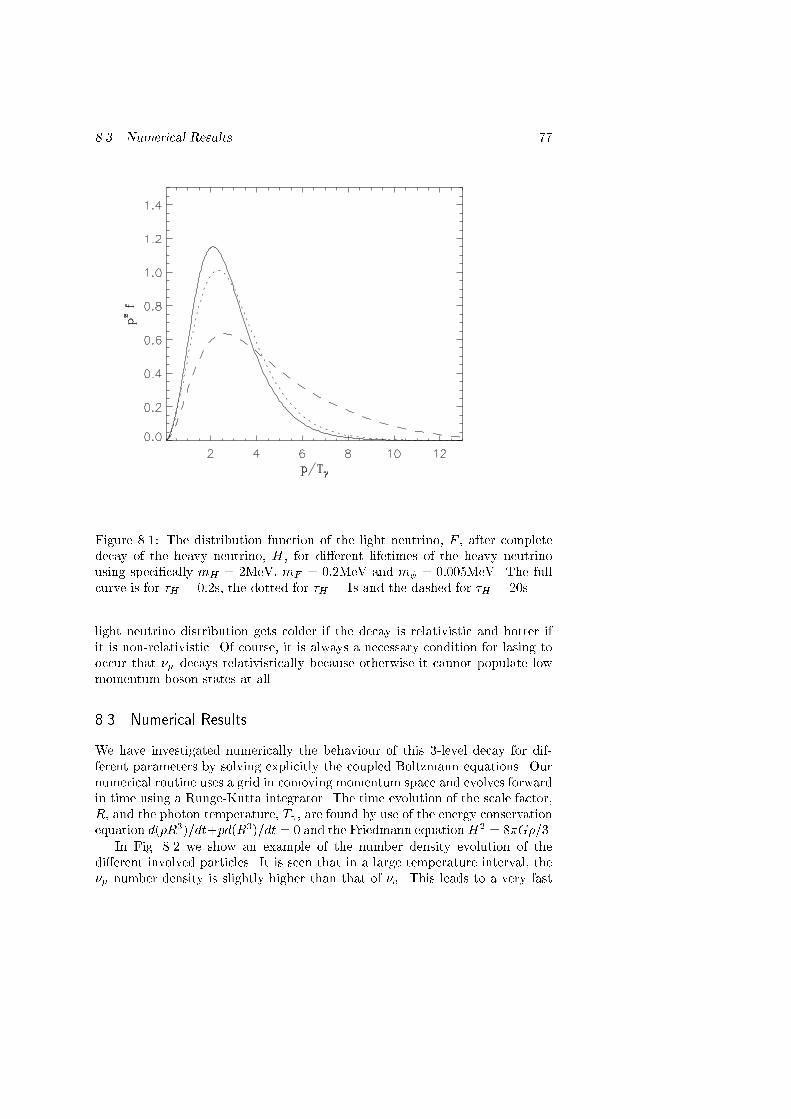
8.3. Numerical Results 77

Figure 8.1: The distribution function of the light neutrino, F , after completedecay of the heavy neutrino, H , for di�erent lifetimes of the heavy neutrinousing speci�cally mH = 2MeV, mF = 0:2MeV and m� = 0:005MeV. The fullcurve is for �H = 0:2s, the dotted for �H = 1s and the dashed for �H = 20s.light neutrino distribution gets colder if the decay is relativistic and hotter ifit is non-relativistic. Of course, it is always a necessary condition for lasing tooccur that �� decays relativistically because otherwise it cannot populate lowmomentum boson states at all.8.3 Numerical ResultsWe have investigated numerically the behaviour of this 3-level decay for dif-ferent parameters by solving explicitly the coupled Boltzmann equations. Ournumerical routine uses a grid in comoving momentum space and evolves forwardin time using a Runge-Kutta integrator. The time evolution of the scale factor,R, and the photon temperature, T , are found by use of the energy conservationequation d(�R3)=dt+pd(R3)=dt = 0 and the Friedmann equationH2 = 8�G�=3.In Fig. 8.2 we show an example of the number density evolution of thedi�erent involved particles. It is seen that in a large temperature interval, the�� number density is slightly higher than that of �e. This leads to a very fast

78 Chapter 8. Neutrino Lasing

Figure 8.2: The evolution of number density for the di�erent involved particles.The full curve is ��, the dotted �e, the dashed �� and the dot-dashed �. Theparameters used are m�� = 2MeV, m�� = 0:5MeV, m� = m�e = 0:005MeV and��� = 0:2s, ��� = 1:0s.growth of the boson number density and is identi�ed with the region wherelasing takes place. The �nal number density of � and �e are the same becauseof neutrino number conservation (neglecting a possible small initial abundanceof �) because even though the �e abundance starts out higher, three �'s areproduced for every two �e.Since both �e and � are almost massless there are essentially four free pa-rameters in our equations. The �rst is the mass scale, de�ned for exampleby the � neutrino mass. This mass scale is unimportant for the shape of thespectra (this is only true if the decays take place below the weak decouplingtemperature Tdec ' 2:3MeV. If the free decay temperature is larger than Tdecthe � distribution will quickly thermalise. Only well below Tdec can the non-equilibrium lasing proceed, but now with an initial thermal � distribution. Inour numerical work we choose that the free decay temperature to be lower thanthe decoupling temperature). In Fig. 8.3 we show an example of changing thenormalisation (m�� ) by a factor of two. This leads to an almost identical �nal

8.3. Numerical Results 79

Figure 8.3: Final boson distribution for two di�erent decay models. The fullcurve is for the parameters m�� = 2MeV, m�� = 0:5MeV, m� = m�e =0:005MeV and ��� = 1:125s, ��� = 18s. The dashed curve is for m�� = 1MeV,m�� = 0:25MeV, m� = m�e = 0:0025MeV and ��� = 4:5s, ��� = 72s. Note thatalthough we have chosen values for m�e and � which is orders of magnitudelarger than the experimental/cosmological limit, this does not in uence the re-sults as long as the values are small compared to all other relevant masses andtemperatures.boson distribution. The other three parameters are��� � � m��3MeV�2 ����1s � (8.11)��� � � m��3MeV�2 ����1s � (8.12)� � m��m�� : (8.13)The �rst two parameters describe how relativistic the free decays of the par-ticles are. A thermal particle shifts from relativistic to non-relativistic at a

80 Chapter 8. Neutrino Lasing

Figure 8.4: The momentum spectrum of � after complete decay for di�erentdecay parameters. The full curve is ��� = 0:09, ��� = 0:01 and � = 0:15. Thedotted is for ��� = 1, ��� = 1 and � = 0:25. The dashed is for ��� = 0:5,��� = 0:5 and � = 0:25. The dot-dashed is for ��� = 1, ��� = 0:03 and� = 0:25. The dot-dot-dot-dashed is for ��� = 0:09, ��� = 1 and � = 0:25. Thelong-dashed is a thermal Bose distribution with the same number density.temperature of roughly T ' m=3. When the Universe is radiation dominatedt1s ' � T1MeV��2 : (8.14)Therefore if the decay is relativistic� < t(T = m=3) ' � m3MeV��2 s: (8.15)Thus, if �i < 1 the decay is relativistic, whereas if �i > 1 it is non-relativistic.The third parameter is just the dimensionless �� mass.Fig. 8.4 shows the �nal boson distribution after complete decay for severaldi�erent choices of decay parameters (for comparison we have also shown athermal Bose distribution with the same number density). It is seen that inorder to get a large fraction of cold particles, we need to have ��� � 1 and

8.3. Numerical Results 81

Figure 8.5: Final momentum distribution of �. The full curve is for ��� = 0:09,��� = 0:03 and � = 0:25. The dotted curve is for ��� = 0:09, ��� = 0:03 and� = 0:15.��� � 1. The reason for this was described in the previous section. Fig. 8.5shows the e�ect of changing the relative mass of the two heavy neutrinos. Wesee here that to get a large cold fraction we also need to have m��=m�� � 1.This is also understandable if we look at the allowed momentum range of theproduced bosons from Eq. (2.42)p��T = 12(1� �2)"sp2��T 2 + m2��T 2 � p��T # : (8.16)If � is close to one we can get very cold bosons. This means that the bosons willtend to cluster in low momentum states, but because of energy conservation weget a very hot �� distribution. On the other hand, if � ! 0, then the lowestboson states are unaccessible and we get instead a colder �� distribution. Thisin turn leads to more lasing in the lasing state and even though the fractionof cold bosons coming from the initial �� decay gets smaller, this is more thancompensated for by the larger fraction coming from the �� decay. This is indeedwhy the cold fraction increases when � decreases.

82 Chapter 8. Neutrino Lasing

Figure 8.6: The temperature evolution of the �-distribution. The decay pa-rameters are ��� = 0:09, ��� = 0:03 and � = 0:25. The dotted curve is atT = 2:3MeV, the dashed at T = 1:1MeV and the dot-dashed at T = 0:5MeV.The full curve is the �nal distribution after complete decay.Thus, if we want to study the region of parameter space with possible in-terest for structure formation scenarios we have essentially limited ourselvesto the region of ultrarelativistic decays with a large mass di�erence betweenthe two heavy neutrinos. It is also interesting to follow the evolution of theboson distributions with temperature to see how the di�erent states populate.Fig. 8.6 shows the temperature evolution of the boson distribution for the decayparameters ��� = 0:09, ��� = 0:03 and � = 0:25.The minimum possible boson energy at a given temperature is given by Eq.(8.16), where instead of �� we use �� and for � we use 0. An approximatelower limit can be calculated by setting p��=T = 3, corresponding roughlyto the mean value from a normal thermal distribution. This lower limit isan increasing function with decreasing temperature and indicates roughly themomentum where the distribution \decouples" (decoupling here means that thestates are kinematically inaccessible) at a given temperature. For the modelshown in Fig. 8.6 we get p�� =T = 0:0039; 0:017; 0:081 for photon temperaturesof 2.3, 1.1 and 0.5 MeV. We see that the lower limit at a given temperature

8.3. Numerical Results 83

Figure 8.7: The temperature evolution of the �� distribution. The decay pa-rameters are as in Fig. 8.6. The full curve is the initial thermal �� distribution.The dotted curve is at T = 2:3MeV, the dashed at T = 1:1MeV and thedot-dashed curve is at T = 0:5MeV.corresponds roughly to the momentum where the distribution decouples. Ofcourse the lower limit will always be somewhat higher than the actual decouplingpoint, but it helps to understand the evolution of the spectra. Fig. 8.7 showsthe corresponding evolution of ��. We see the before mentioned e�ect of ��decay producing a cold �� distribution and thereby enhancing lasing.However, even in the case where the decays are ultrarelativistic and the massratio small, the fraction of cold bosons is only moderate. For example in thecase where ��� = 0:09, ��� = 0:01 and m��=m�� = 0:15, the fraction of bosonswith pH=T < 0:3 is only 44%. If the boson was to act as the dark matterin our Universe, a much larger fraction would be needed. Note, however, thateven if the obtainable cold fraction is too small, it is comparable with or largerthan that obtained in the model of Refs. [16, 67, 72]. Furthermore, it is achievedwithout invoking an unknown neutrino state.

84 Chapter 8. Neutrino Lasing8.4 DiscussionWe have developed further the scenario originally proposed in Refs. [16, 67, 72]by introducing a physically di�erent way of obtaining neutrino lasing. However,this model still su�ers from one of the same shortcomings that the originalmodel did, namely that it is impossible to achieve su�ciently large fractions ofcold bosons for structure formation.An interesting consequence of the 3-level decay is that the number densityof electron neutrinos is increased by a factor of almost three relative to the stan-dard case. If the decay takes place before or during Big Bang Nucleosynthesis(BBN), then it can signi�cantly change the outcome because the electron neu-trinos are very important for the neutron to proton conversion reactions. Thehigher than usual number of electron neutrinos will tend to keep equilibriumlonger than in the standard case, meaning that less neutrons survive to formhelium. The helium abundance will then be lower than in the standard case.Furthermore, the ratio of low energy electron neutrinos is signi�cantly higherthan normal. This favours the neutron to proton reaction because of the massdi�erence between the neutron and the proton and leads to the opposite e�ect ofthe one described by Gyuk and Turner [75], where a massive � neutrino decaysto electron neutrinos, thereby enhancing the neutron fraction and allowing avery high baryon density without violating the BBN constraints. However, intheir scenario, the decaying neutrino is non-relativistic and the resulting electronneutrinos therefore have very high energy (the opposite of our case).Decays producing lasing e�ects are, however, not likely to take place duringBBN. The reason is that neutrinos are kept in equilibrium by the weak reactionuntil roughly T ' 2MeV. All neutrino distributions are then of equilibriumform and no lasing will take place. If the mass of any of the heavy neutrinosis of the same order or larger than this temperature, we will essentially have anon-relativistic decay after decoupling, but this will not produce lasing. Thus,the heaviest neutrino in our scenario must be substantially lighter than 2 MeV,thus making it improbable that it should decay during BBN. In general neutrinodecays a�ecting BBN may well take place, but then they will not produce lasinge�ects. Therefore we have not treated this case in the present paper.If we turn to more speci�c physical models, the most natural candidate forthe light scalar particle, �, is the majoron. There exist several majoron models,all of them designed to explain the very small neutrino masses compared to theother fermions. In the simplest models, the decay �2 ! �1 + � is forbidden attree level [77], making the lifetime too long to be of interest. However, there aremore complicated models where the lifetime can be short. In the simplest casethe majoron couples to the neutrino via a Yukawa interactionL = ig2J�c1 5�2 + h:c: (8.17)From this generic interaction several limits to the coupling strength, g, andtherefore to the lifetime can be derived. For example neutrinoless double �

8.4. Discussion 85decays give an upper limit on g of roughly 10�4 [76]. Other limits can bederived from the neutrino signal of SN1987A [11], but as mentioned in Ref.[11], it is very di�cult to get a clear picture of the current limits. A couplingconstant of 10�4 gives a restframe decay lifetime of [77]� = 32�g2m2 > 10�5s� � m21eV��1 : (8.18)This limit is rather weak and leaves open a large region of parameter space forrelativistic decays in the early Universe. Note that for our model to work thedecay �� ! �e must be suppressed. This corresponds to the coupling g�e beingvery small compared to the other coupling constants.Finally, we have assumed that the scattering and annihilation reactions be-tween neutrinos and majorons are weak compared with the decay reaction. If,as we have assumed, the decay is not forbidden at tree level this is the casebecause the scattering and annihilations all are of order g4, whereas the decaysare of order g2. Were the annihilation and scattering reactions to be impor-tant we would not obtain any cold bosons because the low momentum stateswould not be decoupled. Therefore, it is absolutely necessary that the decaysare stronger than the scattering and annihilation reactions. Note, that even ifthe decay is of order g2 and the scattering and annihilation g4 the decay ratewill be damped by a factor �1 = m=E which can be very large if the decayis extremely relativistic. Thus, in the limit of ! 1 we have to account forscatterings and annihilations, but would have to be extremely large becauseof the very small value of g.As far as the neutrino masses are concerned, they are naturally explainedby see-saw models. Then only the left handed components participate in theinteractions because of the very large mass of the right handed components.The possible Majoron decays are then exactly�i(L) ! �j(L) + � (8.19)�i(L) ! �j(R) + � (8.20)as required in our lasing model.In conclusion, what we have shown is that it is possible to generate large non-equilibrium e�ects, even starting from identical neutrino distributions. Very few\�ne-tunings" are necessary in order to achieve lasing. Thus, these e�ects maybe present many places in early Universe physics, both because the decay typesare generic and because the early Universe is an inherently non-equilibriumenvironment. This was also noted in Ref. [16], but our speci�c model showsthat the relevant range of models is much larger than originally thought. It istherefore of considerable interest to search for other physical scenarios where thelasing process (and other similar non-equilibrium processes) may be e�ective.

86 Chapter 8. Neutrino Lasing

Chapter IXConclusionsIn the present work we have discussed in detail the e�ects of neutrinos on pri-mordial nucleosynthesis. Neutrinos are important in several ways for the way inwhich nucleosynthesis proceeds. First of all they contribute to the cosmic energydensity which in turn controls the expansion rate of the Universe. Furthermorethe electron neutrinos directly enter the weak conversion rates between neu-trons and protons. Since neutrinos in uence nucleosynthesis in such a strongway, primordial nucleosynthesis can be used as an e�ective probe of neutrinophysics.Starting out with physics entirely within the standard model we have per-formed a detailed calculation of the e�ect of neutrinos on nucleosynthesis. Thiscalculation was described in Chapter 5. The point is that, contrary to the usualassumption, neutrinos have not decoupled completely from the cosmic plasmawhen the electrons and positrons annihilate. Therefore they share to some de-gree the entropy transfer that takes place from the e� plasma to the otherspecies. This heats up the neutrino distribution relative to a totally decoupledspecies and in uences nucleosynthesis. The change is minute but neverthelessimportant if one wants to build a very accurate nucleosynthesis code. This typeof calculation has been performed before, but our approach di�ers by the factthat we use the full set of Boltzmann equations without any approximations. Wehave found a somewhat smaller neutrino heating e�ect than the previous state-of-the-art calculation done by Dodelson and Turner [41]. Since our calculationwas performed, new results have appeared by Dolgov, Hansen and Semikoz [51]that con�rm our results. They have used the same approach as us, but withhigher numerical precision.Going beyond the standard model we have looked at neutrinos that aremassive but with lifetime much longer than the timescale for nucleosynthesis.This was done in Chapter 6. Nucleosynthesis limits on massive neutrinos turnout to be complementary to limits obtainable in laboratories and used togetherthey exclude a neutrino mass above ' 0.2 MeV if the neutrino lifetime is longerthan ' 103 s. Again our approach di�ers from earlier calculations in that weuse the full Boltzmann equations. It does turns out, however, that our results87

88 Chapter 9. Conclusionsdo not di�er widely from those obtained by Fields, Kainulainen and Olive [12]who used the integrated Boltzmann equation, but included the correct Fermistatistics for all neutrino species.Since any neutrino with mass above the cosmologically safe limit of roughly100 eV must be unstable with lifetime shorter than the Hubble time, it is naturalto discuss the possibility of neutrinos decaying during nucleosynthesis. Neutrinodecays can be split into a few generic types. Especially there is a di�erencebetween the case where decay products interact electromagnetically and the casewhere they are \invisible". There exist very strong limits on the �rst type ofdecay, making it extremely unlikely that these decays should play any role duringBBN. However, this is not the case for the second type of decay. Such decayshave been discussed in detail, most recently by Dodelson, Gyuk and Turner[40]. However, their approach is to use the integrated Boltzmann equation ina non-relativistic approximation. For neutrinos decaying su�ciently late, whenthey have already become non-relativistic, this is a very good approximation.For relativistic or semi-relativistic decays this not the case. Here one needs tostudy the full Boltzmann equation since there can be signi�cant deviations fromkinetic and chemical equilibrium. This has been done previously for the verysimple decay �� ! ��� by Kawasaki et al. [59, 68]. In Chapter 7 we presentedthe calculation for the case of of �� ! �e�, which is much more complicatedbecause the decay product electron neutrinos enter into the conversion processbetween neutrons and protons, as previously mentioned. In our calculation wehave found signi�cant quantitative di�erences between our calculation and thoseperformed with the non-relativistic approximation. We have also discussed thepossibility that a low mass tau neutrino decaying with short lifetime to anelectron neutrino �nal state can bring nucleosynthesis predictions into betteragreement with observations.Lastly we have looked at a neutrino process which is somewhat more exotic,namely that of neutrino lasing. The fundamental idea was originally introducedby Madsen [67] who studied a possible stimulated decay of some neutrino speciesinto a neutrino plus scalar particle �nal state. If this stimulated decay proceedsin equilibrium it gives rise to the possibility of forming a Bose condensate of thedecay product bosons. This could potentially be very interesting for models ofstructure formation in the early Universe. The reason is that both cold and hotdark matter is apparently needed to �t observations of the present day largescale structure. By having the above mentioned stimulated decay, some of thebosons are in a Bose condensate whereas the rest are in a thermal distribution.If this boson has a small mass it can act as both cold and hot dark matter,thereby explaining these mixed dark matter models with only one new particle.The problem is, however, that only a relatively small fraction of the bosons endup in the condensate, roughly 35%, whereas a fraction closer to 70% is needed to�t observational data. The scenario was calculated through in more detail usingBoltzmann equation formalism by Starkman, Kaiser and Malaney [16]. Theyfound that a true Bose condensate does not form, but that instead there will bea peak of very low momentum bosons in a \pseudo-condensate". The fraction

89of particles in this low momentum peak is roughly the same as that found byMadsen for the equilibrium decay; that is, much too small to be interesting forstructure formation.We have developed a new scenario for the lasing decay using only equilibriuminitial distributions. The trouble for the original scenario was that an initialpopulation inversion is needed between the heavy and light neutrino. Otherwisethe stimulated decay is never initiated and the �nal distribution is thermal.Originally this population inversion was invoked by having the light neutrinodecouple very early (prior to the QCD phase transition) so that its abundancewould be diluted by the entropy released in the subsequent phase transition.However, if there is a three neutrino mass hierarchy we have shown that itis possible to achieve lasing with just the three known neutrino species. Inthis scenario the heaviest neutrino acts as the pumping level in a normal threelevel laser, whereas the next species in the hierarchy is the actual lasing level.When the heaviest species decays while still relativistic it produces a populationinversion between the �rst and second generation so that a lasing mechanismoccurs naturally. We have presented thorough calculations of this scenario inChapter 8. It was found that the amount of cold bosons produced is not muchhigher than in the original scenario so that the model is still not viable as anexplanation of mixed dark matter. However, it does show that the range ofmodels where the lasing phenomenon can occur is much larger than originallythought.In conclusion, the present work has presented detailed calculations of someof the physical mechanisms that can take place during or close to the era ofBig Bang Nucleosynthesis. It was found that neutrinos play a very importantrole for the evolution of our Universe, and that cosmological observations cantherefore be used to probe neutrino physics in regions that terrestrial experi-ments cannot reach. However, there are still signi�cant problems, for examplethe observational determinations of the primordial abundances are still quiteuncertain. This again means that primordial nucleosynthesis is still not at asu�cient level of precision that one may start discussing constraints on �ne-points in the input physics. This issue will hopefully be resolved in the comingfew years as the observations of for example QSO absorption systems are im-proved. By determining the deuterium abundance accurately one should be ableto pin down the baryon-to-photon ratio very precisely so that �rm predictionscan be made for the abundance of the other light elements. We should then bein a position to really start testing the physical composition of the Universe atan age of seconds using Big Bang nucleosynthesis.Finally, a few words should perhaps be said about a possible new approachto determining the fundamental cosmological parameters, namely from the mea-suring of small scale anisotropies in the cosmic microwave background. This willbe done within the next few years by two satellites, the American MAP and theEuropean PLANCK (formerly known as COBRAS/SAMBA) missions.According to expectations these should be able to perform a precision mea-surement of the uctuation amplitude beyond the �rst Dopplerpeak, thereby

90 Chapter 9. Conclusionsenabling an accurate determination of cosmological parameters like �, H , etc.This would yield a value for � independent of nucleosynthesis arguments, sothat the �eld of Big Bang nucleosynthesis would enter a new precision era bymeans of this external input.

Chapter XOutlookThere are a number of issues which have not been addressed at all in the presentwork that may be very interesting for future work. The �rst is entirely withinthe standard model and deals with the precision to which one can really predictthe helium abundance theoretically. During the past year or two, more andmore emphasis has been put on the need to really understand the theoreticaluncertainties in the nucleosynthesis calculations. This point is especially con-cerning when one looks at 4He because this is probably the only light elementwhere we can ever hope to measure the primordial abundance to su�cient ac-curacy. There are a number of uncertainties in the standard nucleosynthesiscalculations that need to be addressed. This was �rst discussed by Dicus etal. [43] some 15 years ago and since then there has been an increasing numberof calculations of these e�ects. Primarily, the error in the standard calculationcomes from neglect of �nite nucleon masses. The neutrino heating e�ect dis-cussed in Chapter 5 is another example of a missing element. However, thereare many more such �ne-points, like medium e�ects etc. The normal calculationassumes that all processes proceed in vacuum which is of course not true. Manythings are changed when physical processes occur in a dense medium, for ex-ample normally massless species like neutrinos and photons acquire an e�ectivemass. Even though many of these e�ects are minute they are still interestingfrom a theoretical point of view and may improve our understanding of physicsin the early Universe.Another important issue is the possibility of neutrino oscillations duringprimordial nucleosynthesis. This is of course potentially important for massiveneutrinos such as a heavy tau neutrino. Especially if electron neutrinos areinvolved in the oscillations, one can obtain quite large e�ects on nucleosynthesis.Last, if we look at neutrino physics more generally it would also be veryinteresting to do studies of neutrinos in the supernova environment. This �eldis somewhat disjoint from neutrino physics in the early Universe; however, manyof the techniques applied are similar. Also, what we can learn from studyingneutrinos in supernovae is in many ways complementary to what one can learnfrom neutrino physics in the early Universe. For this reason this type of study is91

92 Chapter 10. Outlooka very interesting future prospect. In many ways the supernova environment isnot nearly as well understood as the early Universe. Supernova physics couplesa lot of complicated phenomena together in an almost intractable way andprocesses such as the transport of neutrinos in a very dense medium are notwell understood from a theoretical perspective. Thus, a lot of work remains tobe done in this �eld. For instance, presently the precise mechanism that leadsto the visible supernova blast instead of complete collapse to a black hole is notunderstood, but is believed to be connected with the way neutrinos propagatethrough the medium surrounding the young neutron star.

AcknowledgementsThere are a great number of people to whom thanks are due. First of all I wishto thank my thesis supervisor Jes Madsen for his guidance during the years andfor making me choose this �eld of work by being such an inspiring lecturer.The help and guidance of Georg Ra�elt has been invaluable and he alsomade possible my stay at the Max Planck Institut f�ur Physik in Munich for sixmonths during 1997.There are a number of people at the Institute of Physics and Astronomywhom I also wish to thank for interesting discussions and good company ingeneral, my o�ce mates Michael Christiansen and Georg B. Larsen as well asmy other friends at the institute.Del-B of my Ph.D. study has been �nanced by the Theoretical AstrophysicsCenter under the Danish National Research Foundation and they have alsoagreed to hire me after I have �nished my Ph.D.In the non-physics community I wish to thank my parents for all their sup-port and especially my friend Jesper who has been very good at keeping mefrom doing physics all the time. Thanks also to all my other friends.

93

94

Appendix AMathematical FormalismA.1 Dirac Matrices and Their AlgebraThe Dirac matrices are de�ned from the Dirac equation for a free particle( �p� �m) = 0; (A.1)and they obey the commutation relations (Cli�ord algebra)f �; �g = 2g�� : (A.2)From these matrices one can de�ne the a matrix, 5, as 5 � i 0 1 2 3; (A.3)where 5 obeys the relations 25 = 1 (A.4)and f 5; �g = 0; (A.5)so that 5 is its own inverse and furthermore it anticommutes with all the other -matrices.Several di�erent representations are used for the Dirac matrices, depend-ing on convenience in a given calculation. The standard choice is the Diracrepresentation where 0 = � I 00 �I � i = � 0 �i��i 0 � ; (A.6)and 5 = � 0 II 0 � : (A.7)The matrices �i are the usual Pauli spin matrices de�ned as�1 = � 0 11 0 � �2 = � 0 �ii 0 � �3 = � 1 00 �1 � : (A.8)95

96 Appendix A. Mathematical FormalismOther choices than the Dirac representation are possible, for example thechiral representation in which 0 = � 0 �I�I 0 � i = � 0 �i��i 0 � : (A.9)In this representation 5 is 5 = � I 00 �I � : (A.10)There are many di�erent such representations which may be chosen for conve-nience in a given situation.Another quantity which is often important is the commutator between Diracmatrices ��� = i2 [ �; � ]; (A.11)which has the properties � � = g�� � i��� (A.12)and [ 5; ��� ] = 0: (A.13)A.2 Dirac SpinorsFor free particles the solutions to the Dirac equation have the form of planewaves of positive and negative energy +(x) = ue�ip�x (A.14) �(x) = veip�x; (A.15)where u and v are Dirac spinors that are themselves solutions to the Diracequation ( �p� �m)u = 0 (A.16)( �p� +m)v = 0: (A.17)Explicitly these spinors are given byu(p; s) = pE +m� �s��pE+m�s � ; (A.18)v(p; s) = pE +m� ��pE+m�s�s � ; (A.19)where �s is a two-component spinor �eld. s is the helicity which can be �1=2.Therefore the spinor �s can assume the values�+ = � 10 � �� = � 01 � (A.20)

A.3. Creation and Annihilation Operators 97This gives the normalisationuys(p)us0(p) = 2E�ss0 (A.21)vys(p)vs0(p) = 2E�ss0 (A.22)vys(p)us0(p) = 0; (A.23)of the Dirac spinors.A.3 Creation and Annihilation OperatorsThe fermion creation and annihilation operators (fy and f) as well as the cor-responding operators for antiparticles (fy and f) are de�ned so as to obey theanti-commutation relationsff(p; s); f y(p0; s0)g = �ss0�(p� p0) (A.24)ff(p; s); f y(p0; s0)g = �ss0�(p� p0); (A.25)with all other anti-commutators being zero. The action of the creation andannihilation operators on physical states has the following e�ectf(p; s)jp; si = j0i (A.26)fy(p;s)j0i = j(p; s)i (A.27)f(p; s)jp; si = j0i (A.28)fy(p;s)j0i = j(p; s)i; (A.29)where by j0i we mean the vacuum state.

98 Appendix A. Mathematical Formalism

Appendix BPhase-space IntegralsThis appendix shows how to reduce the integral in Eq. (2.29) from 9 to 2 dimen-sions. Except for the inclusion of mass terms, most of what can be found in thisappendix was originally developed by Yueh & Buchler [78] for use in supernovacalculations.The collision integrals all have the form of Eq. (2.29). The innermost integralcan be rewritten using the equalityd3p42E4 = d4p4�(p24 �m24)�(p04): (B.1)The integral over d4p4 is now done using the �-function. Hereafter p4 is �xed asp24 = p21 + p22 + p23 + 2(p1 � p2 � p1 � p3 � p2 � p3): (B.2)Now, the following angles are introducedcos� = p1 � p2p1p2 (B.3)cos � = p1 � p3p1p3 (B.4)cos�0 = p2 � p3p2p3 (B.5)= cos� cos � + sin� sin � cos�:Thus we obtain d3p2 = p22dp2d cos�d� (B.6)d3p3 = p23dp3d cos �d�: (B.7)The integration over d� is carried out using the �-function. We use thatp24 �m24 = f(�): (B.8)99

100 Appendix B. Phase-space IntegralsFrom the standard theory of �-functions we useZ d��(f(�)) =Xi Z d� 1���df(�)d� ����=�i �(� � �i); (B.9)where �i are the roots of f(�) = 0. The derivative is evaluated todf(�)d� = �2p2p3 sin� sin � sin�: (B.10)sin�i is found as �(1� cos2 �i)1=2, wherecos�i = 2E2E3 � 2p2p3 cos� cos � �Q2p2p3 sin� sin � (B.11)� (2E1E2 � 2p1p2 cos�)2p2p3 sin� sin �+(2E1E3 � 2p1p3 cos �)2p2p3 sin� sin � ;and we have introduced Q = m21 +m22 +m23 �m24. The equation for sin�i willhave two solutions, one in the interval [0; �], and one in the interval [�; 2�].Since the r.h.s. of Eq. (B.9) is symmetric in � we can multiply by two andintegrate over [0; �]. The limits on the integral d cos� come from demandingthat cos2(�) � 1. But this means that(2p2p3 sin� sin � sin�)2 � 0: (B.12)Notice, that this is the same as demanding that�df(�)d� �2 � 0: (B.13)Finally we end up withZ 2�0 d��(f(�)) = 2 1���df(�)d� ����=�i� ����df(�)d� ����2�=�i! : (B.14)The derivative can be written as����df(�)d� �����=�i =pa cos2 �+ b cos�+ c; (B.15)where a = p22(�4�+ 8�) (B.16)b = p2(p1 � �=p1)(8 + 4Q+ 8�) (B.17)c = �4 2 � 4 Q�Q2 � 8 �� 4Q�� 4�2 (B.18)+4p22p23(1� cos2 �);

101and we have introduced the following parameters in order to limit the amountof space required to write out the formulae = E1E2 �E1E3 �E2E3 (B.19)� = p1p3 cos � (B.20)� = p21 + p23: (B.21)Notice that Eqs. (B.16), (B.17) and (B.18) reduce to those of Yueh & Buchler[78] in the limit of zero masses.Now, any one of the possible matrix elements only include products of 4-momenta. All the possible products of these momenta are calculated below:p1 � p2 = E1E2 � p1p2 cos� (B.22)p1 � p3 = E1E3 � p1p3 cos � (B.23)p1 � p4 = m21 + (E1E2 � p1p2 cos�) (B.24)�(E1E3 � p1p3 cos �)p2 � p3 = (E1E2 � p1p2 cos�) (B.25)�(E1E3 � p1p3 cos �) +Q=2p2 � p4 = (E1E3 � p1p3 cos �) +m22 �Q=2 (B.26)p3 � p4 = (E1E2 � p1p2 cos�)�m23 +Q=2: (B.27)Because all the above products are analytically integrable over d cos�, the in-tegrals over this parameter can now be carried out by use of the fundamentalrelation Z 1�1 dxpax2 + bx+ c�(ax2 + bx+ c) = �p�a�(b2 � 4ac) (B.28)The step function comes from demanding that there be a real integration inter-val. This actually also insures that the roots of ax2+ bx+ c are not outside thefundamental integration interval of [�1; 1], because the step function singles outthe physical situations, where d cos� can not be outside this interval. Integrat-ing over d� is no problem, as there is no dependency on this parameter. The�nal integration that can be done is the one over d cos �. Any one of the possi-ble products of momenta is analytically integrable over d cos �. The solution ofb2 � 4ac = 0 gives the integration interval. The solutions arecos � = (�2 � 2p22 �Q (B.29)�2p2(2 + p21 + p22 + p23 +Q) 12 )=(2p1p3):If there is to be a real integration interval, both of these solutions must bereal. The fundamental interval is of course [�1; 1], but the real limits are � =sup[�1; cos �min] and � = inf[1; cos �max]. There can only be a real integrationinterval if both � and � are real numbers and � � �.

102 Appendix B. Phase-space IntegralsNote that there are seemingly two places where divergences occur in thecollision integral. The �rst one is for p1 = p3; cos � = 1, but in this case thereis no problem because although the integrand becomes in�nite it is integrablyin�nite [78]. The second place is for p1 ! 0. To see what happens here, we haveto go back to the fundamental integral, Eq. (B.28). If p1 ! 0 then a = �4p22p23,but then there can be no divergence, as p1 no longer appears in any denominator.Clearly there is still the possibility of divergence if m1 ! 0 also, because of the1=E1 term. Fortunately it turns out that b2 � 4ac = 0 if m1; p1 = 0, so thatthe rate becomes equal to 0 in this case, as it ought to be. Finally the collisionintegral can be written asCcoll[f ] = 2(2�)4 12E1 Z p22dp22E2 p23dp32E3 S � (B.30)�(f1; f2; f3; f4)F (p1; p2; p3)�(A);where A is the parameter space allowed (that is, the space de�ned by requiring�; � real and � � �). F is the matrix element integrated over d cos� and d cos �,F (p1; p2; p3) = Z jM j2 d cos�d cos � (B.31)

Appendix CEnglish Resum�eThe goal of the present work has been to investigate aspects of the interfacebetween particle physics and cosmology. This �eld is one of the most promisingin the whole area of modern physics, since in many cases the whole Universe canbe used as a giant particle physics laboratory. We have focused on the particlescalled neutrinos and their importance in the early Universe. Neutrinos areweakly interacting spin-1/2 leptons, essentially equivalent to electrons exceptfor the fact that they apparently do not possess either mass or electric charge.Three generations of neutrinos are known to exist, �e, �� and �� , correspondingto the charged leptons e, � and � . Since neutrinos interact so weakly, very littleis actually known about them. They are extremely di�cult to detect in thelaboratory even though they are present in great abundance everywhere, beingproduced continuously by for example the Sun. For this reason, one must oftenturn to indirect means of studying neutrinos. One such possibility is to use theearly Universe as a neutrino laboratory.There is no a priori reason why neutrinos should be completely massless,and a large part of this thesis has been devoted to the study of massive neu-trinos in cosmology. It turns out that neutrinos are intimately connected withthe formation of light nuclei when the Universe was about 1 second old, thephenomenon usually referred to as Big Bang Nucleosynthesis (BBN). Studies ofthe outcome of BBN can therefore tell us a lot about the properties of neutrinos.Features that are completely unreachable in terrestrial laboratories.The �rst four chapters of the thesis have been devoted to an introduction tothe fundamental concepts needed. Chapter 1 is a general introduction, Chap-ter 2 contains a discussion of the evolution equations for the expansion of theUniverse as well as a review of the Boltzmann equation, the fundamental trans-port equation relating di�erent particle species in the early Universe. Chapter3 reviews Big Bang Nucleosynthesis, both the theoretical and the observationalaspects. In the theoretical section the in uence of neutrinos and other particleson nucleosynthesis is discussed. In the observational part we look at how thedi�erent light element abundances are observed as well as discuss the problemsconnected with these observations. In Chapter 4 the physics of neutrinos is103

104 Appendix C. English Resum�ediscussed. We start out with the de�nitions of quantum neutrino �elds anddiscuss the weak interactions of neutrinos, emphasising the similarities and dif-ferences of Dirac and Majorana neutrinos. In the �nal section neutrino decaysare discussed, primarily the experimental constraints that exist on such decays.In the next four chapters we proceed with a more speci�c discussion of neu-trino physics in the early Universe. Chapter 5 contains a thorough calculation ofthe in uence of massless standard model neutrinos on primordial nucleosynthe-sis. We �nd that the neutrinos distributions are heated slightly relative to thestandard calculations because energy is transferred from electrons and positronsas these become non-relativistic and annihilate. Our calculation has been morecareful than previous ones, taking into account the full quantum statistics ofneutrinos. After our results appeared, new and numerically more precise resultsby Dolgov, Hansen and Semikoz have appeared that con�rm our results.Chapter 6 goes beyond the minimal standard model in that neutrinos areallowed to have mass. However, we still assume that they only possess standardmodel weak interactions and furthermore we assume their lifetime against de-cay to be su�ciently long not to have any e�ect on nucleosynthesis (� � 103s).Massive neutrinos a�ect primordial nucleosynthesis quite dramatically, mainlybecause their non-zero rest mass energy can come to dominate the cosmic en-ergy density at temperatures below the rest mass. This again changes the cosmicexpansion rate and generally leads to a strong increase in helium production.We �nd that tau neutrinos with mass larger than roughly 0.2 MeV are ruledout by combining our nucleosynthesis arguments with the laboratory mass limitof 24 MeV for the tau neutrino. This is consistent with previous results, butour treatment has included use of the full Boltzmann equation, following eachmomentum mode in time instead of the usual approach where one assumes scat-tering equilibrium for the involved neutrinos. Our calculations were performedfor Majorana neutrinos only, but the limits can be expected to be roughly thesame for Dirac neutrinos, also ruling out a massive Dirac neutrino if its restmass is larger than roughly 0.2 MeV, still assuming a su�ciently long lifetimeagainst decay.In Chapter 7 we proceed to look at the possibility of neutrino decays duringnucleosynthesis. This phenomenon has been discussed many times in the liter-ature, but we look at one very interesting range in parameter space that has sofar not been treated properly, namely that of a low mass tau neutrino decayingto an electron neutrino �nal state. For the last few years there have been someindication that the standard picture of BBN may be lacking something. Theproblem is that apparently too much helium is produced to be consistent withobservations. A decay of the type we discuss can help solve this problem sinceit lowers the helium abundance from nucleosynthesis if the mass and lifetime ofthe decaying neutrino are both su�ciently low. Again, we have used the full setof Boltzmann equations as opposed to previous treatments. For the speci�c de-cay we look at, this is the only way to obtain sensible results because the decaydoes not necessarily install equilibrium in the particle distributions. We havefound a large range of allowed neutrino decay lifetimes for masses in the range

1050.1-1 MeV. As in the previous chapter we only looked at Majorana neutrinosbecause there are several additional complications for Dirac neutrinos.Lastly, in Chapter 8 we have looked at a di�erent aspect of neutrino physicsin the early Universe. Here we study the possibility of making dark matterfrom neutrino decays. Dark matter is the generic term for the mass knownto be present in the Universe, but not identi�able as normal baryonic matter.This matter is for example needed to produce the present day structure ofthe Universe, such as galaxies etc. It turns out that to be consistent withobservations most of the dark matter should be in very heavy particles, calledcold dark matter. However, a small fraction of light particles is needed, termedhot dark matter. Some years ago it was suggested by Madsen that this type ofscenario could possibly be produced by stimulated decay of massive neutrinosto a �nal state containing some scalar particle. It turned out, however, that therelative fraction of cold and hot dark matter was wrong, most of the dark matterended up in the form of hot dark matter. We have developed this scenario toa new model with more than one neutrino decay, but it still appears that toomuch hot dark matter is produced.

106 Appendix C. English Resum�e

Bibliography[1] G. F. Smoot et al., Astrophys. J. Lett. 396, L1 (1992).[2] See for example R. Giovanelli and M. P. Haynes, in Annual Review ofAstronomy and Astrophysics 29, 499 (1991).[3] G. Gamow, Phys. Rev. 70, 572 (1946).[4] Much more extensive information can be found in recent reviews such asH. Reeves, Rev. Mod. Phys. 66, 193 (1994); R. A. Malaney and G. J.Mathews, Phys. Rep. 229, 145 (1993); M. S. Smith, L. H. Kawano and R.A. Malaney, Astrophys. J. Suppl. 85, 219 (1993).[5] S. Burles and D. Tytler, Report no. astro-ph/9603070.[6] K. A. Olive and D. Thomas, Astropart. Phys. 7, 27 (1997).[7] R.M. Barnett et al. (Particle Data Group), Phys. Rev. D 54, 1 (1996).[8] N. Hata et al., Phys. Rev. Lett. 75, 3977 (1995).[9] J. Bernstein, Kinetic Theory in the Expanding Universe, Cambridge Uni-versity Press (1988).[10] S. Weinberg, Gravitation and Cosmology, John Wiley and Sons (1972).[11] G. G. Ra�elt, Stars as Laboratories for Fundamental Physics, Universityof Chicago Press (1996).[12] B. D. Fields, K. Kainulainen, and K. A. Olive, Report no. hep-ph/9512321(1995). 107

108 Bibliography[13] R. V. Wagoner, in Physical Cosmology - Les Houches (1979), edited byR. Balian, J. Audouze and D. N. Schramm, Les Houches Summer SchoolProceedings Vol. 32, p. 395.[14] P. Gondolo and G. Gelmini, Nucl. Phys. B360, 145 (1991).[15] K. Kainulainen and A. D. Dolgov, Nucl. Phys. B402, 349 (1993).[16] G. D. Starkman, N. Kaiser and R. A. Malaney, Astrophys. J. 434, 12(1994).[17] K. A. Olive and G. Steigman, Astrophys. J. Suppl. 97, 49 (1997).[18] Y. I. Izotov, T. X. Thuan and V. A. Lipovetsky, Astrophys. J. Suppl. 108,1 (1997).[19] A. Songaila et al., Nature (London) 368, 599 (1994).[20] M. Rugers and C. J. Hogan, Astron. J. 111, 2135 (1996).[21] J. K. Webb et al., Nature 388, 250 (1997).[22] D. Tytler, S. Burles and D. Kirkman, Report no. astro-ph/9612121.[23] F. Spite and M. Spite, Astron. Astrophys. 115, 337 (1982).[24] P. Bonifacio and P. Molaro, Mon. Not. R. Astron. Soc. 847, 285 (1997).[25] see for example J. Bahcall, talk given at 18th Texas Symposium on Rela-tivistic Astrophysics, Chicago IL, Report no. astro-ph/9702057.[26] See for example T. K. Gaisser, Talk given at the 17th International Con-ference on Neutrino Physics and Astrophysics (Neutrino 96), Helsinki, Fin-land, Report no. hep-ph/9611301.[27] C. Athanassopoulos et al., Phys. Rev. Lett. 77, 3082 (1996).[28] K. Grotz and H. V. Klapdor, The Weak Interaction in Nuclear, Particleand Astrophysics, Adam Hilger 1990.

Bibliography 109[29] K. Assamagan et al., Phys. Rev. D 53, 6065 (1996).[30] D. Buskulic et al., Phys. Lett. B 349, 585 (1995).[31] B. Kayser, F. Gibrat-Debu and F. Perrier, The Physics of Massive Neutri-nos, World Scienti�c Lecture Notes in Physics - Vol. 25 (1989).[32] D. Bailin and A. Love, Introduction to Gauge Field Theory, Adam Hilger1986.[33] R. Plaga, Report no. hep-ph/9610545 (1996); S. Hannestad, Report no.hep-ph/9701216 (1997); B. Kayser, Reoprt no. hep-ph/9703294 (1997); A.Hoefer, Report no. hep-ph/9705362 (1997); S. H. Hansen, Report no. hep-ph/9708359 (1997).[34] see the paper by R. Plaga in Ref. [33].[35] P. Vilain et al. (CHARM II collaboration), Phys. Lett. B335, 246 (1994).[36] E.W. Kolb and M.S. Turner, The Early Universe, Addison Wesley (1990).[37] P. J. E. Peebles, Principles of Physical Cosmology, Princeton UniversityPress 1993.[38] see for example A. L. Mellott and D. W. Sciama, Phys. Rev. Lett. 46, 1369(1981).[39] see for example R. N. Mohapatra and P. B. Pal, Massive Neutrinos inPhysics and Astrophysics, World Scienti�c Lecture Notes in Physics -Vol. 41 (1991).[40] S. Dodelson, G. Gyuk and M. S. Turner, Phys. Rev. D 49, 5068 (1994).[41] S. Dodelson and M.S. Turner, Phys. Rev. D 46, 3372 (1992).[42] A. D. Dolgov and M. Fukugita, Phys. Rev. D 46, 5378 (1992).[43] D. A. Dicus et al., Phys. Rev. D 26, 2694 (1982).

110 Bibliography[44] M. A. Herrera and S. Hacyan, Astrophys. J. 336, 539 (1989).[45] N. C. Rana and B. Mitra, Phys. Rev. D 44, 393 (1991).[46] S. Hannestad and J. Madsen, Phys. Rev. D 52, 1764 (1995).[47] L. Kawano, Report no. FERMILAB-Pub-92/04-A (1992) (unpublished).[48] B.D. Fields, S. Dodelson, and M.S. Turner, Phys. Rev. D 47, 4309 (1993).[49] C. J. Copi, D. N. Schramm, and M. S. Turner, Phys. Rev. Lett. 75, 3981(1995).[50] R. Cowsik and J. McClelland, Phys. Rev. Lett. 29, 669 (1972).[51] A. D. Dolgov, S. H. Hansen and D. V. Semikoz, Preprint no. TAC-1997-10,Report no. hep-ph/9703315.[52] For recent reviews, see G. Gyuk and M. S. Turner, Nucl. Phys. B Proc.Suppl. 38, 13 (1995); G. Gelmini and E. Roulet, Rep. Prog. Phys 58, 1207(1995).[53] D. A. Dicus et al., Phys. Rev. D 17, 1529 (1978).[54] E. W. Kolb and R. J. Scherrer, Phys. Rev. D 25, 1481 (1982).[55] R. J. Scherrer and M. J. Turner, Ap. J. 331, 19 (1988).[56] A. D. Dolgov, K. Kainulainen and I. Z. Rothstein, Phys. Rev. D 51, 4129(1995).[57] E. W. Kolb et al., Phys. Rev. Lett. 67, 533 (1991).[58] A. D. Dolgov and I. Z. Rothstein, Phys. Rev. Lett. 71, 476 (1993).[59] M. Kawasaki et al., Nucl. Phys. B419, 105 (1994).[60] A. D. Dolgov, S. Pastor, and J. W. F. Valle, Report no. hep-ph/9602233(1996).

Bibliography 111[61] S. Hannestad and J. Madsen, Phys. Rev. Lett. 76, 2848 (1996).[62] J. Bernstein, L. S. Brown and G. Feinberg, Phys. Rev. D 32, 3261 (1985).[63] In the published version of Ref. [48] the same e�ect will be accounted for,with very good agreement with our results (Kimmo Kainulainen, privatecommunication).[64] N. Terasawa and K. Sato, Phys. Lett. B 185, 412 (1987).[65] E. W. Kolb and R. J. Scherrer, Phys. Rev. D 25, 1481 (1982).[66] R. J. Scherrer and M. S. Turner, Astrophys. J. 331, 19 (1988); R. J. Scherrerand M. S. Turner ibid. 331, 31 (1988).[67] J. Madsen, Phys. Rev. Lett. 69, 571 (1992).[68] M. Kawasaki, K. Kohri and K. Sato, Report no. astro-ph/9705148.[69] S. Hannestad and J. Madsen, Phys. Rev. D 54 7894 (1996).[70] C. J. Copi, D. N. Schramm, and M. S. Turner, FERMILAB-Pub-94/174-A(1994).[71] Recent treatments are M. Kawasaki, G. Steigman, and H.-S. Kang, Nucl.Phys. B403, 671 (1993); G. Gyuk and M. S. Turner, in Neutrino 94, Pro-ceedings of the 16th International Conference on Neutrino Physics and As-trophysics, Eilat, Israel, edited by A. Dar et al. [Nucl. Phys. Proc. Suppl.B 38, 13 (1995)].[72] N. Kaiser, R. A. Malaney, and G. D. Starkman, Phys. Rev. Lett. 71, 1128(1993).[73] See for example A. Klypin, J. Holtzman, J. Primack, and E. Reg�os, Astro-phys. J. 416, 1 (1993).[74] G. B. Larsen and J. Madsen, Phys. Rev. D 53, 2895 (1996).

112 Bibliography[75] G. Gyuk and M. S. Turner, Phys. Rev. D 50, 6130 (1994).[76] Z. G. Berezhiani et al., Phys. Lett. B 291, 99 (1992).[77] See for example C. W. Kim and A. Pevsner, Neutrinos in Physics andAstrophysics, Harwood Academic Publishers (1993).[78] W. R. Yueh and J.R. Buchler, Astrophysics & Space Science, 39, 429(1976).