neuro-genetic system for stock index prediction
TRANSCRIPT

Neuro-genetic system for stock index prediction
Jacek Mandziuk1 and Marcin Jaruszewicz2
1 Faculty of Mathematics and Information Science,
Warsaw University of Technology,
Plac Politechniki 1, 00-661 Warsaw, Poland
Abstract
This goal of the paper is introduction and experimental evaluation of neuro-genetic
system for short-term stock index prediction. The system works according to the
following scheme: first, a pool of input variables are defined through technical data
analysis. Then GA is applied to find an optimal set of input variables for a one day
prediction. Due to the high volatility of mutual relations between input variables,
a particular set of inputs found by the GA is valid only for a short period of time
and a new set of inputs is calculated every 5 trading days. The data is gathered
from the German Stock Exchange (being the target market) and two other markets
(Tokyo Stock Exchange and New York Stock Exchange) together with EUR/USD and
USD/JPY exchange rates.
The method of selecting input variables works efficiently. Variables which are no
longer useful are exchanged with the new ones. On the other hand some, particu-
larly useful, variables are consequently utilized by the GA in subsequent independent
prediction periods. The proposed system works well in cases of both upward or down-
ward trends. The effectiveness of the system is compared with the results of four other
models of stock market trading.
Key words: financial forecasting, stock index prediction, neuro-genetic system, neural
networks, genetic algorithms, time series analysis, trend prediction, technical analysis,
oscillators, pattern extraction.
Published in
Journal of Intelligent & Fuzzy Systems, 22(2), 93-123, 2011, IOS Press
1

1 Introduction
Trade decisions on a stock market are made on the basis of predicting the trend and
are driven by many direct and indirect factors. Effective decisions depend on accurate
prediction.
Many techniques applied to the task of stock market prediction are presented in the
literature. First of all, different models of a stock market are constructed. For example, the
fundamental analysis is used to define models which calculate the future price according
to current indicators [14]. The estimation of the current value of the company is used to
predict future changes of the price. Data mining methods are applied to the problem of
identification of rules existing on a stock market. These rules are also used to predict the
future price [33, 46].
A different goal is stated for models which reflect the functioning of stock markets [58].
Building the stock market model helps finding the mechanisms and instruments for pre-
diction [26]. Mathematical models are also used to construct optimal portfolios [2, 56, 71].
One of the oldest and the most popular is Black and Sholes Model [45, 51, 65], initially
proposed in [5]. A more complicated model of a stock market, which reflects various types
of investors’ behavior is presented in [47].
Computational Intelligence (CI) methods are widely used for stock market predic-
tion. In case of neural networks in the majority of published papers either feed-forward
or recurrent neural models are applied. In case of feed-forward architectures, both sig-
moidal [11, 24, 31, 32, 74] and radial basis [8, 27, 39, 49, 73] neurons can be used. In
order to discover and take advantage of changing relations between stock market indicators
various recurrent networks are considered, as well, e.g. [38, 49, 63, 68]. Another popular
direction is the use of support vector machines [8, 9, 23, 25], introduced by Vapnik [69, 70].
Application of neural networks usually requires appropriate data preparation before
the learning process can commence. Data preprocessing methods consider dividing data
into specific subsets according to either direction of a trend [11] or based on statistical
properties of the data [16, 40]. The methods of classification and segmentation can also be
used directly to predict future values [1]. Also transformations of input records aiming at
data decorrelation are applied. The most popular methods include PCA [9] and ICA [9,
10, 12].
As an alternative to CI methods, statistical models can be used. Usually either the
Markov models [3, 4, 36, 65, 68] or more sophisticated, based on analysis of variance,
ARIMA and GARCH models [35, 54] are considered. The question concerning the superi-
ority of CI methods over statistical models (or vice versa) is still open although according
to some papers (e.g. [41]) the efficacy of ARIMA or GARCH is not satisfactory compared
to neural networks or SVMs. Please refer to [27, 68] for experimental comparison and
2
discussion.
Most of the neural methods described above require specific set up of steering pa-
rameters and suitable selection of the input data. Both these issues can be effectively
approached with the help of genetic algorithms (GAs). For example, in [67] the authors
propose a system for stock market prediction relying on neural networks and fundamental
analysis, where the selection of variables is performed by the GA.
Alternatively, the topology of the network or its internal parameters can be determined
by the GA [21, 29, 37, 44].
GAs are also applied to the task of generation of optimal prediction rules/models [17,
33, 34, 46] or transformation of the knowledge hidden inside neural network’s weights to
a self-explanatory set of rules [18].
Despite remarkable effort devoted to stock market prediction, the problem remains
difficult and in general case unsolved. The main reason for this difficulty are complex and
varying in time dependencies between factors affecting the price [59, 67]. According to
some theories, changes on stock markets are chaotic [54]. The Efficient Market Hypothesis
(EMH) says that all available information (or only past prices in the weak variant of the
hypothesis) is already reflected in the current price. Therefore it is not possible to predict
future values. Several researches deny this hypothesis. In [66] the authors formulated
the problem equivalent to the EMH. In short, if the hypothesis were true it would not
be possible to find any structure in the data allowing for efficient compression. In order
to deny the EMH such compression algorithm was proposed in the paper. Consequently,
since the compression is possible, the data must be somehow structured, ergo the task of
prediction is worth undertaking. The EMH was also questioned by applying statistical
tests to NYSE returns [50].
Another task, which might question the EMH is the issue of discovering correlations
between prices on different stock markets. The common statistical test for detecting
dependence in time series is Brock–Dechert–Scheinkman test (BDS) [6]. BDS was, for
example, used to discover the existence of non-linear correlations on Shanghai (SHSE)
and Shenzen (SZSE) stock markets [42]. In [55] the matrix of mutual correlations between
several stock markets - before and after the 1987 crash - was calculated and used to prove
the existence of correlations between European and US stock markets.
Analysts who are professionally involved in stock prediction use both fundamental and
technical analysis data. The former considers objective (fundamental) reasons for the
price changing including economical indicators or political situation on both country and
company level. The latter relies on specific transformations and visual interpretation of the
past market data, especially prices and volumes. In CI literature, both fundamental [14,
47, 60] and technical [13, 17, 60] analysis driven articles can be found.
3

1.1 Research goals
This paper is a continuation and extension of our prior works [31, 32, 52, 53] bringing
several new results and deeper analysis. Preliminary results were obtained with one neural
network using a narrow range of variables. The outcomes were promising and deeper
analysis was conducted. Along with adding new variables, the architecture of the system
developed. In response to an increasing number of potential input variables and changing
in time dependencies between them, the genetic algorithm was implemented for selection
of the most efficient subset of inputs for neural network based predictors. The final form of
the proposed system includes several original ideas invented by the authors, which extend
the capabilities of the “canonical” neuro-genetic approach.
The following three hypotheses are formulated and experimentally verified in the stud-
ies presented in this paper. The first one claims that appropriately designed prediction
system composed of simple neural networks supported by a genetic algorithm is able
to deliver a reliable short-term prediction of an index value. The remaining two hy-
potheses verify human expert knowledge concerning the stock market investment: the
first one states that there exist correlations between stock markets; the second one as-
sumes that relations between factors influencing an index value (i.e. technical indicators,
max./min./opening/closing index values, averages, oscillators, etc.) change in time. In
other words, efficient prediction of an index value requires that the set of input values
used for prediction varies in time.
1.2 An overview of the proposed prediction system
The general idea of the prediction system proposed in this paper is to form a suitable com-
bination of the computational power of neural networks with flexibility and optimization
capabilities of genetic algorithms. The goal is to predict the closing value of German Stock
Exchange (GSE) index DAX for the next day. The approach relies solely on technical anal-
ysis data. Except for the target market, the data from two other international markets,
namely American New York Stock Exchange (NYSE) with DJIA index and Tokyo Stock
Exchange (TSE) with NIKKEI 225 (NIKKEI) index are also considered, together with
exchange rates of EUR/USD and USD/JPY.
Variations in time dependence between variables related to these three markets are
also taken into account. The most suitable set of input variables is chosen by the GA
and validated by a simplified neural network training and testing procedure. Due to high
volatility of mutual dependencies between input variables the set chosen by the GA is only
used for 5 trading days. After this period a new set of variables is chosen for the next 5
trading days, and so on.
The proposed solution combines the power of the GA in a wide and parallel search with
4

the intrinsic ability of neural networks to discover relations within input data. The system
works without human intervention by choosing desired input variables autonomously from
a large number of possibilities. In independent prediction steps, the algorithm selects vari-
ables in a sensible way, generally consistent with human trading knowledge. The existence
of characteristic, repeatable patterns of variables within subsequent 5-day windows can be
observed (see Section 6.4 for a detailed discussion).
Whilst the GA was probing different sets of variables several interesting observations
were made. For example, the existence of chromosomes in a population, that coded neural
networks unable to learn was discovered. We refer to these chromosomes as dead. They
were present especially in early iterations of the GA. The algorithm tended to consequently
eliminate dead chromosomes (see Section 3.2 for details).
Our specification of GA allowed differentiation of the sizes of input variables sets. This
made the prediction system flexible to changing situations on the stock market. Results
obtained during a series of experiments are encouraging. The return of an investment
achieved by the proposed model of trading visibly exceeds the buy and hold strategy
(a simple trading strategy consisting in buying stocks on the first day of the assumed
trading period, and selling them all on the last day of the trading period, with no other
transactions in between). The model also outperformed two other simple investment
strategies implemented for comparison.
1.3 Relation to the literature
There are plenty of papers devoted to stock market prediction with the use of neural
networks, genetic algorithms, or a combination of both these paradigms. Some examples
of such papers are cited above in order to illustrate the variety of possible approaches.
However, to our knowledge, there are not many papers closely related to the goals under-
lying this work, i.e. the use of GA for input variable pre-selection based on the data from
(presumably) correlated sources (the three, geographically distinct stock markets in here),
to be subsequently used by a neural network based predictor. Actually, the only paper
that we were able to trace, in which a similar idea of applying the GA for input variables
pre-selection, is authored by Kwon, Choi and Moon [43], where the goal is to predict the
company’s stock price. However, unlike in our approach, the authors of [43] consider the
companies which are correlated with the target one, but belong to the same stock mar-
ket (the Korea Stock Exchange). From the initial pool of variables the GA discovers the
approximately optimal input set for the recurrent Elman neural network (RNN) [19]. A
selected set of variables is used for testing period of one year. Afterwards a new set of
variables is proposed. The authors show the advantage of the proposed system over RNN
that uses fixed set of variables concerning the target company only, and over the buy and
hold strategy.
5

In our approach, on the other hand, the effectiveness of neuro-genetic system is further
augmented by considering technical data from other stock markets, as well as using narrow
5-day time window, which forces frequent exchange of selected variables.
The remainder of this paper can be described as follows. The next section contains
a description of the methods of data transformation used in the paper. Calculations of
statistical variables, oscillators, and applied pattern recognition methods are presented.
Analysis of dependencies between different variables is also provided. In Section 3 com-
ponents of the proposed system are described in detail. The main elements of the system
(neural networks and GA) and the extensions of standard GA implementation intended
for this research are described in detail. Section 4 provides definitions of five different ap-
proaches to trading on the stock market considered in the paper for comparison purposes.
The investment goal is defined as the value of return of invested amount of money. One of
the models is based on a proposed neuro-genetic prediction system. Another three models
rely on simple heuristics. The last approach, referred to as prophetic, assumes possessing
the knowledge of the future movement on the stock market. This system, by its definition,
achieves the highest possible return in the current situation on the market. As a summary
of research concerning the proposed hybrid prediction model, four different parameters’
settings are specified in Section 5. The superior one is chosen for the final experiment. In
Section 6 numerical results of performed experiments are provided and compared in terms
of obtained returns. Analysis of variables chosen by GA and used in subsequent prediction
periods is presented and discussed. The issues concerning stability and repeatability of
results are also considered in this section. The paper ends with conclusions and directions
for future research.
2 Data analysis
In this section a data preparation step is described. It starts with analysis of plain values
of an index, proceeds with defining averages and oscillators, and ends with application of
pattern extraction techniques. Since the goal is defined as a one-day prediction, fundamen-
tal analysis is not very helpful [57]. Instead, the main focus is on technical analysis and its
indicators. Another possibility would be the use of portfolio management methods, which
also proved to be efficient in short-term prediction [15, 33]. The source data consists of
the opening, highest, lowest and closing values of the index of the selected stock markets
in subsequent days. This data serves as the basis for further transformations, e.g. the
percentage change of opening value through the last 5, 10 and 20 days or the averages of
opening values through the last 5, 10 and 20 days.
The above variables are intuitively useful for prediction. They provide simple presen-
tation of past values in a compressed way. Especially moving averages allow the algorithm
6

to omit sudden local changes when looking for prediction rules. The predefined periods
for averages and changes (5, 10, 20 days) were chosen based on preliminary simulations
and suggestions from the literature [64]. Generally speaking these periods need to be
adjusted to the assumed prediction horizon, which is equal to 1 day in this paper. The
same time periods are also used in more complex transformations, e.g. in definitions of
the oscillators.
Figure 1: Closing DAX value and its changes in the period 2004/04/07 to 2004/08/26.
A chart of index values with corresponding changes in the period April 7, 2004 –
August 26, 2004 is presented in Fig. 1. Sudden up and down changes can be observed.
On the other hand, general rises and falls of trend are also clearly visible.
On the above basis the oscillators, known in technical analysis, are calculated [57].
The following oscillators are chosen in our experiment: MACD; Williams; Two Averages;
Impet; RSI; ROC; SO and FSO. The above set of oscillators was constructed manually
among the most popular ones, frequently used in real stock trading. Except for raw
values, the buy/sell signals generated by the oscillators are also considered. For example,
the MACD and Williams oscillators are defined by equations (1) and (2), resp.
MACD = mov(C, 10)−mov(C, 20), MACDSIGNAL = mov(MACD, 5) (1)
7

where C is the index closing value and mov(X,n) denotes the moving average of vari-
able X in the last n days. Signals are generated at the intersections of MACD and
MACDSIGNAL.
WILLIAMS(n) =max(H,n)− C
max(H,n)−min(L, n)(−100) (2)
where n is a period of time (set to 10 days in the paper), max(H,n),min(L, n) are the
highest and the lowest index value in this period, respectively. C is index closing value.
According to technical analysis the use of oscillators is, besides chart analysis, one of
the main methods of effective investing [61, 64]. Several examples from the literature con-
firm the efficacy of using the oscillators [22, 30, 72] on stock or currency exchange markets.
Therefore this data is a relevant part of the whole range of potential input variables. An-
other useful method of trend prediction is pattern analysis. Several characteristic patterns
can be observed in the index value chart. Their extraction is based on local minima and
maxima values. The algorithm of pattern extraction used in our experiment is described
later in this section. An alternative interesting implementation of an algorithm of pattern
extraction is presented in [13]. The most common patterns are: head and shoulders, tri-
angles, bottoms and apexes. Some of them forecast change of prediction, others confirm
the actual trend. This property defines two types of patterns according to either holding
or changing the trend. Selected patterns are presented in diagrams shown in Fig. 2.
In order to recognize such structures first of all local minima and maxima of index
values are calculated. A special parameter called “fill coefficient” controls the definition
of the localness which influences the number of extracted minima and maxima. Two
parameters (similarity and difference) define the meaning of closeness of values. Two
values will be treated as similar if the difference between them is smaller than the similarity
coefficient. Two values will be treated as not equal if the difference between them is greater
than the difference coefficient. Based on these conditions it is possible to compare different
tops and bottoms of an index chart. Extraction of the technical analysis patterns is based
on matching the schema of actual tops and bottoms with the built-in schema of predefined
patterns.
Figure 3 shows an example of pattern extraction of test samples (B - recognized min-
ima, S - recognized maxima). Double bottom and three apexes are found in the presented
range of data. Due to the ambiguity of the method two different patterns concern one set
of sample records, but both of them forecast the change of the trend. Each pattern found
is coded by the respective integer number and added to the training records. Aside from
the pattern itself, the type of it (holding or changing the trend) is also included in the
training data. Together with the day of the week of prediction and different variants of
specific oscillators there are 37 variables describing the index value and its derivatives on
8

(a) triangle (b) double apex (c) head and shoulders
Figure 2: Examples of technical analysis patterns.
one stock market (per day) which are taken into account.
Figure 3: Pattern extraction from the test sample. B, S denote recognized minima andmaxima, resp.
2.1 Dependencies between variables
A situation on a particular stock market usually depends on other markets. It is a sort of
communicating vessels. Therefore the dependencies between variables from different stock
markets were measured. The Pearson correlation coefficient (eq. (3)) was used to measure
the linear correlation between variables:
lcPearson =
n−1∑i=0
(xi − x)(yi − y)√n−1∑i=0
(xi − x)2n−1∑i=0
(yi − y)2
(3)
where n is the number of available records. The higher the value, the stronger the
relation between x and y.
Two charts (presented in Figs. 4 and 5) show relationships between the change of
closing value of the target stock market and other variables from the considered stock
markets. In Fig. 4 correlations of all variables of three stock markets (GSE (with DAX),
TSE (with NIKKEI) and NYSE (with DJIA)) are shown. Some characteristic patterns are
9

visible in GSE and NYSE sets. The same patterns are also present in TSE data but with
much smaller magnitude. This confirms the existence of correlation between different stock
markets especially European and American ones. The importance of several variables is
noticeable. Variables most likely correlated with predicted changes of closing value are
oscillators and changes of closing values from other stock markets.
Figure 4: Correlation between variables of stock markets: value of change of DAX vs.other variables.
Despite strong relations between variables, dependencies change in time. In Fig. 5 a
correlation between the closing DAX value and the MACD oscillator on the target stock
market is presented. On x-axis a sequence of a 5-day time-windows is placed. The period
of 470 days sub-divided into 94 pieces is considered. For every piece the correlation is
calculated. The correlation can be either positive or negative, either strong or weak. It is
difficult to find appropriate prediction rules that would be valid through the whole range
of data. Variability of dependencies must be taken into account. The method of variables
selection must be sensitive to market’s volatility in the above described sense.
Except for the linear correlations between variables from different stock markets the
underlying structure of the time series composed of the predicted variable’s values is
also examined. The BDS test rejects the hypothesis that examined sample is a series
of independent and identically distributed random variables (see Table 1 for details).
Test sample consisted of 2420 values of percentage one-day changes of stock market’s
closing index values. The rejection of null hypothesis indicates the existence of non-linear
correlations in the data.
10

Figure 5: Correlations between input factors: value of change of DAX vs. MACD on GSE.
3 Components of the prediction system
A large number of variables were available after the data preparation step described in
Section 2. A method of selecting an approximately optimal, in the current situation, set of
variables and a neural network-based predictor which uses them as the input are described
in subsections below. The final selection of the input variables is performed by the GA.
Each chromosome codes a set of input variables to be used by a neural network. A fitness
function is reverse-proportional to the magnitude of an error made by a trained network
on a sample test set. After the GA finishes its work the best fitted chromosome provides
a suitable set of variables to be used in the final training. These variables are considered
to be an optimal selection for the current 5-day window.
3.1 Neural networks
Neural networks form the basis of the proposed prediction system. Feed-forward networks
with one hidden layer are chosen based on preliminary experiments. The size of the hidden
layer equals the floor function of the half of the size of an input layer (e.g. in case of 9
input neurons, the hidden layer is composed of 4 units). One neuron is used in the output
layer. Therefore the architecture of each network used in the system during the GA phase
or for the final prediction is defined completely by the number of input variables. The
11

ϵ Dimension (m) Statistic P-value
0.008 2 9.4726 < 2.2e-16
0.008 3 15.9697 < 2.2e-16
0.016 2 10.2794 < 2.2e-16
0.016 3 16.7567 < 2.2e-16
0.024 2 10.2981 < 2.2e-16
0.024 3 15.9623 < 2.2e-16
0.033 2 9.7885 < 2.2e-16
0.033 3 14.5233 < 2.2e-16
Table 1: Results of BDS test for 2420 samples representing the percentage one-day changesof closing DAX index values. The results were calculated with the help of the “R” statis-tical package [62].
weights of such a network are randomly initialized.
The method of back propagation with momentum is used for training, which is per-
formed for a pre-defined number of epochs (see Section 5 for the choice of the training
parameters). Changes of network’s weights are defined by the following equation:
∆wk = µk(−∂Qk
∂wk) + α∆wk−1 (4)
where Q is a mean square error of network’s output, µk - a learning coefficient, w - a
vector of weights, k - an iteration number. The first part of the right hand side of equation
(4) is a standard back propagation method of changing weights in the learning process.
The second part - momentum, lets the learning to consider also the previous direction
of a change, despite the actual gradient. Both components require suitable choice of
coefficients. In each training epoch the value of the learning coefficient µk may change
within a predefined range, which is one of the system’s parameters (listed in Section 5).
The training procedure was stopped (in iteration t) based on the fulfillment of one of
the following conditions:
t = tmax (5)
or
MSEt > MSE1 (6)
or
∀k=0,1,2 1− SumMSEt−k−1
SumMSEt−k≥ 0.1, (7)
where
SumMSEn =
i=9∑i=0
MSEn−i (8)
12

denoted the sum of the MSE errors from the last 10 iterations. Condition (6) was true
when a NN defined by the chromosome was unable to learn (the chromosome was dead).
The third condition was used to detect three consecutive increases of the sums of the MSE
errors over 10 last epochs. The number of epochs was equal to 10 was used in order to
smooth individual MSE changes in single epochs. Parameter tmax was equal to 200 or
2000 depending on the stage of the algorithm (see Section 5 for details).
3.2 Genetic algorithm
The neural network training process is efficient if the size of the network is relatively small.
This goal is typically achieved by adaptation of network’s topology [20, 21, 28, 48].
Another possibility of optimization is efficient selection of input variables. In order to
select small, but relevant number of variables for a neural network the GA is applied. Due
to a large number of available input variables and changing dependencies between them,
a selection of a suitable subset of inputs is the main idea of the proposed system. The
quality of prediction strictly depends on the effectiveness of the GA. The chromosome
is defined as the list of variables used by a neural network for training and prediction.
Therefore each chromosome defines a specific network’s architecture, as described in the
previous subsection. For example if a chromosome codes the following set of variables:
closing value of DAX, average change in 20 days, MACD oscillator value, percentage
change in 20 days, then the network defined by this chromosome has 4 input neurons, 2
neurons in a hidden layer and 1 output neuron. For each input neuron the value of the
respective variable is provided. The fitness function is reverse-proportional to the error of a
network after training. The smaller the error on validation samples, the higher the fitness
of a chromosome. For each chromosome several neural networks with different initial
weights, but the same architecture are considered. The fitness function can be calculated
with respect to either the minimum or the average error of all networks assigned to the
chromosome. If the average error is used the algorithm is less sensitive to accidental
increase or decrease of the learning process effectiveness caused by the initial weights
choice.
Sometimes during training, for the specific set of input variables, the network is unable
to achieve acceptable level of an error. This usually happens in the initial population of
chromosomes, but sometimes also in further generations, when some of the variables are
not suitable for learning. Chromosomes which code such useless sets are called dead. The
remaining chromosomes are called alive.
There are two main operators in the GA. A crossover is responsible for creating new
chromosomes using information coded by both parents. Mutation brings random changes
in chromosomes, which expand their capabilities of searching for the result in the whole
solution space.
13

Two crossover methods are implemented in the proposed system. The first one is
classical crossover with one cutting point. The cutting point can by selected randomly or
chosen according to the best fitness of the resultant child chromosome (see Fig. 6). The
alternative crossover method, a combined crossover [7], depends on the common part of
two parent chromosomes and random selection of the rest of variables. The scheme of the
combined crossover is presented in Fig. 7. This kind of crossover promotes variables that
are repeated in the population.
Figure 6: The scheme of the classical crossover operation with one cutting point.
Figure 7: The scheme of the combined crossover operation with a random selection ofvariables. V1, V2, V3, V4 are randomly selected from the remaining pool of variables (i.e.except for X and Y ) with additional condition that they are pairwise different within eachof the chromosomes, i.e. V1 = V2, V2 = V3 and V3 = V1.
In any case, two offspring are created as a result. Selection of chromosomes for crossover
is performed by the rank method. A parent is exchanged with assigned child only if the
latter one is better fitted. Using the above described crossover does not alter population
14

size. Sizes of individual chromosomes generally change towards the preferred/winning
ones.
During mutation variables coded by the chromosome are exchanged with variables
chosen randomly from the remaining subset of all available ones. A single mutation can
affect only one randomly selected variable.
Both crossover and mutation operators have the assigned probability of occurrence.
For crossover it equals 1 because the decision of replacing parents with children is done
later based on values of their fitness. Probability of mutation depends on the type of
chromosome. Probability for dead chromosomes is greater than for alive ones. This
setting forces the undesirable chromosomes to be changed. Changes in alive chromosomes
are rare - just enough to keep the diversity of the population. The exact values of these
parameters are discussed in Section 5.
Selection of new variables in crossover and mutation is performed from the current
pool of available variables, which is a subset of all possible variables. More precisely,
since the set of all possible variables is too large to form an initial pool for the GA (there
are 370 variables, concerning the current and past days, from the three stock markets
under consideration), before the GA starts, the initial pool is selected either by using
the autocorrelation method (considering the rank of correlation with the closing value of
DAX) or manually.
The main drawback of selection based on the autocorrelation is that in order to be
effective it must consider a long-range of historical data. Hence the method is not sensitive
to short-term, local correlations, which are crucial for effective market modeling. There-
fore, in the final experiments described in this paper, the manual method of selecting the
initial pool of variables was used.
Manual selection takes into consideration all variables from the target stock market
(70 variables), last day changes of closing values of the two other stock markets and the
two exchange rates. All together, a set of 74 variables is chosen and available for the use
of the GA.
The first step of the GA is creation of the initial population. Variables coded by
chromosomes are randomly selected from the initial pool. Diversity of the population
is assured by creating chromosomes of different sizes (numbers of coded variables). All
chromosomes’ sizes from a predefined range are represented in the initial population.
In each iteration of the GA new chromosomes are created as a result of crossover and
mutation. Gradually the average error of prediction made by neural networks coded by
the chromosomes decreases.
After every iteration the best chromosome is appointed. A chromosome can be con-
sidered the best one only if all neural networks used in the fitness evaluation are able to
learn (is alive for every network). The number of such networks is one of the system’s
15

parameters (see Section 5 for details). Finally, in the last iteration of the GA the network
with the lowest error for the best chromosome is saved and subsequently used in the final
test.
3.3 Modifications of the genetic algorithm
Except for “standard GA implementation” described in the previous section several ex-
tensions are proposed and examined. Most of them affect a direction of exploration of the
solution space. They also control sizes of the chromosomes in the population.
The freedom of choosing variables for each chromosome is restricted by forcing the
presence of the last change of the closing index value on target stock market. This forced
variable is not affected by mutation and is present in each chromosome. This “unorthodox”
setup of the GA was strongly supported by the intuitive assumption that the most relevant
variable (i.e. the one having the highest correlation with the predicted variable) is the
target variable obtained in the previous time step. This commonsense idea was positively
verified in preliminary experiments, which besides confirmation of this fact also indicated
that imposing similar restriction on other variables may lead to deterioration of results.
Choosing a new variable during mutation or crossover takes place according to specific
probability. The selection probability depends on the history of variable’s occurrence
in the population. There are three types of variables: best chromosome, often selected,
common. Variables which were present in any of the former best chromosomes have the
type best chromosome variable. Variables which appear in the population more frequently
than the average appearance are called often selected variables. The rest of variables are
common ones. For each type of variables there is a different probability of selection during
mutation or crossover. The probability for best chromosome variables is higher than for
often selected ones. The lowest probability of selection is for common variables. As the
GA starts, probabilities for all variables are pairwise equal. After some predefined number
of iterations probabilities are redefined to 1, 0.75, 0.5 for best chromosome, often selected
and common variables, resp. and assigned to variables in respective categories (types).
Type assignment to each variable is redone at the beginning of every iteration.
Different selection probabilities of variables are applied to enhance variables treated by
the GA as more important. Preliminary experiments showed that this mechanism visibly
accelerates the convergence of the GA, not having a negative influence on diversity of the
population.
When the average error of the whole population approaches the minimum error by
less than 3%, the probability of mutation increases in order to enhance diversity of the
population.
For the sake of increasing the GA’s ability to explore a wider range of solution space
the optional split of the population is implemented. If the split option is selected, in some
16

predefined number of initial iterations crossover is performed within two separated halves
of a population. Additionally, during this initial period of evolution the probability of
mutation is relatively high. Under the above conditions the population rapidly changes
in two separated instances for a predefined period of time. Afterwards the probability of
mutation decreases assuring higher stability of the population. Results of experimental
verification of this method of population split are presented in Section 6.
Sizes of chromosomes may change during the crossover when parents are exchanged
with children, since a parent is exchanged with that child which inherits the size from the
other parent (see Figs. 6, 7). Thus the mechanism of controlling sizes was implemented.
If the average size of chromosomes becomes close to the current maximum or minimum
size in the population, the mutation of chromosomes’ sizes is applied with probability
psize (defined below). If the average size of chromosomes is close to the maximum, the
mutation adds a randomly selected variable to the chromosome. Otherwise a randomly
chosen variable is removed from the chromosome. In both cases, the goal is to support
the current trend of size changes. The probability of the size mutation psize is defined by
eq. (9):
psize = pbaseMaxfitness − chromosomefitness
Maxfitness −Minfitness(9)
with predefined base probability pbase, where Maxfitness and Minfitness denote re-
spectively the maximum and minimum chromosome’s fitness within the population. Also
in this case the probability of selecting variables to be added or removed is considered
according to their type (best chromosome, often selected, common).
A specific extra improvement procedure based on the brute forcemethod is applied after
the last iteration of the GA. In a single iteration of this additional procedure the local
optimality of the winning (best fitted) chromosome is experimentally verified by checking
all possible replacements of one of its variables with anyone else from the remaining pool
of variables. Each new chromosome created this way differs from the original (best)
chromosome by only one variable. The chromosome with the best fitness value among
these newly created chromosomes is compared with the hitherto best chromosome. The
one of them which is better fitted is considered to be the best chromosome. The number of
iterations of this extra improvement can be set a priori or can, for example, be proportional
to the length of the best chromosome. In all experiments reported in this paper the number
of these additional iterations was set to one.
3.4 Stopping conditions
The basic stopping condition for the GA and neural network learning is the number
of iterations. For neural networks there is also the stopping condition dependant on
17

validation samples. If, during training, the error on validation samples rises, the process
is interrupted.
There are two additional stopping conditions for the GA. The first one controls the
diversity of the population according to the average fitness. If the majority of chromosomes
is close to the average fitness the algorithm stops. The second stopping condition applies
if the number of iterations without finding the new best chromosome exceeds a predefined
value.
A general overview of the entire system is presented in Fig. 8.A more detailed descrip-
tion of the method’s implementation, in the form of a pseudocode is placed in Appendix
1.
Figure 8: A general overview of the system.
In the next two sections the efficiency of proposed prediction system is validated.
First of all some comparative models are defined. A simplified investment game on a
stock market is proposed as a verification of their effectiveness.
18

4 Comparative models
In order to examine the effectiveness and usefulness of proposed system of prediction four
other models of stock market’s game were implemented for comparison.
All models are based on generating buy/sell signals to make the maximum future return
of transactions on index value. There are two general assumptions: 1) it is assumed that
there is no handling charge; 2) the index has the price equal to its current value. In the
initial state there is a fixed budget for transactions. At the end of the day the signal for
the next day is generated. Transaction is generated with the next day’s opening value.
If the signal is buy as many indices as possible with the current budget are bought. The
remaining money (the amount smaller than the cost of one index) stays in the budget. If
the sell signal is generated by the system all possessed indices are sold. The total budget
is available for future transactions. The final result of the investment is the total budget
after selling all indices in the last day.
Definitions of determination of signals for all implemented models are placed below.
Model 1 - buy and hold strategy: the first day’s signal is buy, the last day’s one is sell,
and there are no other buy/sell signals generated (eq. (10)):
if(iteration = first) signal = buy
if(iteration = last) signal = sell
if(iteration <> first and iteration <> last) signal = wait
(10)
As a result the return is proportional to the change of an index value in a given time
period.
Model 2 - signals are generated assuming that the direction of a change of an index value
in the following day will be the same as the last day’s change direction (eq. (11)):
if(last change is positive) signal = buy
if(last change is negative) signal = sell
if(last change is zero) signal = wait
(11)
Model 3 - signals are calculated using the next day’s prediction of proposed neuro-genetic
system (eq. (12)):
if(predicted change is positive) signal = buy
if(predicted change is negative) signal = sell
if(predicted change is zero) signal = wait
(12)
Model 4 - signals are calculated using a popular MACD oscillator (see Section 2). Signals
are generated at the crossing of lines of the oscillator (eq. (13)):
19

if(MACDt ≥ MACDtSIGNAL) and (MACDt−1 < MACDt−1
SIGNAL) signal = buy
if(MACDt ≤ MACDtSIGNAL) and (MACDt−1 > MACDt−1
SIGNAL) signal = sell
otherwise signal = wait
(13)
where MACD and MACDSIGNAL are described by eq. (1), t and t − 1 denote time
steps.
Model 5 - signals are generated using the actual knowledge of the next day’s value.
This model yields the highest theoretically possible result under defined conditions of
investment:
if(actual future change is positive) signal = buy
if(actual future change is negative) signal = sell
if(actual future change is zero) signal = wait
(14)
In summary, Model 3 is based on a prediction provided by our neuro-genetic system.
Other models are implemented for comparison purposes. Models 1 and 2 are constructed
using simple heuristics with no particular prediction system. Model 4 is based on a well-
known MACD oscillator. Model 5 defines the theoretical upper limit of a return of an
investment that can be achieved. It takes advantage of the future next day’s index value
(yet unknown in real situation), assuming its availability beforehand.
5 Experiment scenario
A single experiment is divided into steps. Each step consists of neural network training on
290 samples and 5 validation records. The number of training samples is chosen to cover a
year of observations. On the other hand it is a reasonable number of samples for training
the average-size neural network used in the proposed system. The neural network selected
in the current step is tested on the subsequent 5 records not used in previous phases. In
the next step the process is repeated using samples shifted by 5 records. Large part of the
data is shared between steps since in subsequent ones the time-window is only shifted by
5 days forward (test samples from immediately previous step become validation ones and
validation samples become the last part of the training days). The scenario of selection of
learning, validation and testing records in subsequent steps is presented in Fig. 9. A 5-day
period of using the same set of input variables is chosen according to some intuition and
also due to technical reasons. After 5 trading days the GA can be easily run during the
weekend to provide a new input variables’ selection for the next week (5 trading days).
Four different experiments, each consisting of 20 steps were performed in order to
present usefulness of the above approach. In effect, in each experiment the consistent
20

Figure 9: A schema of learning, validation and testing samples selection.
set of 100 (20 × 5) samples was considered as the test data (covering the period from
2004/04/07 to 2004/08/26 - cf. Fig. 1). In each step the following sequence of activities
was performed: A: creating initial pool of variables, B: finding the best chromosome by
the GA, and C: performing the final training with neural network and input variables
coded by that chromosome.
Common parameters of all experiments are described below, grouped according to
the above activities. Parameters, especially probabilities of mutations were chosen in
preliminary experiments so as to achieve desired dynamics of changes in the population.
The size of a population is a compromise between diversity and efficiency of the GA.
A: The initial pool of variables is selected manually and consists of the following
variables: all variables from the target stock market for the current day (30 variables),
moving averages and changes of all index values from the target stock market for past
days (40 variables), changes of closing index value in two other stock markets and two
exchange rates (4 variables).
B: The GA runs on the following parameters:
• population size = 48 chromosomes,
• maximum number of generations = 500,
• initial chromosomes sizes between 3 and 10 (plus one forced variable),
• chromosomes encoding one hidden layer networks only,
• the number of neural networks used to calculate fitness of each chromosome = 3,
• the best chromosome only if all neural networks are alive,
• one iteration of extra improvement after the GA terminated,
• maximum number of iterations during neural network learning for fitness calculation
in GA = 200,
21

• the probability of mutation if not alive = 1,
• the probability of mutation if the average fitness is close to the minimum fitness =
0.2,
• the probability of mutation if alive, before parameters’ change = 0.2,
• the probability of mutation if alive, after parameters’ change = 0.05,
• one variable is changed in one mutation,
• allow mutation of alive chromosomes, if the number of them is greater than 90% of
the population size,
• forbid mutation of alive chromosomes, if the number of them is below 50% of the
population size,
• use a separate set of parameters for the first 20% of iterations.
C: The final neural network learning depends on the following parameters:
• maximum number of iterations during learning = 2000,
• the learning coefficient is changing within the range [0.1, 0.8],
• the value of the learning coefficient is renewed before each iteration,
• the momentum coefficient = 0.2.
All the above choices of exact values or ranges of particular parameters used in the final
experiments reflect the compromise between the desire for the highest possible efficiency of
the system and its time complexity. For the sake of practical applicability the simulation
time of a single run should not exceed 48 hours (on a single processor PC), since the
choice of variables is valid for 5 trading days only and need to be re-calculated over the
weekend. This was the main reason for keeping the population size and the number of
GA’s generations relatively low. Likewise, neural architectures used for chromosomes’
assessment were very simple, with the restricted size of the input layer (the number of
variables in a chromosome) and small numbers of training epochs. Only the final training of
the ultimate neural network was performed in the more time-consuming regime. In general,
system’s parameters were chosen rationally based on a limited number of preliminary tests.
Hence, the above choice by no means should be treated as optimal, although it constitutes
a kind of “local maximum” in the parameter space (with respect to the data granulation
used in the preliminary tests).
Aside from the above settings, some specific parameters are used in each experiment.
These parameters are presented in Table 2 and explained and motivated in the following
section.
22

Parameter Exp. 1 Exp. 2 Exp. 3 Exp. 4
X cross-type cross-type combined-type combined-type
Y yes yes yes no
Z increases decreases decreases decreases
Table 2: Parameters of four experiments. X - denotes type of crossover (cross-type orcombined-type), Y - splitting population in the initial 20% of GA’s iterations, Z - changingin time of the neural network learning coefficient.
5.1 A typical pass of the algorithm
Before presentation of the experimental results let us visualize variations in GA inter-
nal parameters (minimum, average, maximum chromosome fitness (Fig. 10), minimum,
average, maximum chromosome size (Fig. 11), and the number of parent chromosomes’
exchanges with the offspring (Fig. 12)) in a typical step of the algorithm.
Figure 10: Minimum (lower line), average (middle line), and maximum (upper line) fitnessof chromosomes in subsequent generations in one step of the experiment.
In the example the first 20% (i.e. 100) of GA’s iterations were performed with a sep-
arate set of parameters having a high probability of mutation, equal to 0.2. Before the
38th iteration (see Fig. 10) the population was rapidly developing better and better chro-
mosomes. Afterwards, there was a period of stabilization when, despite relatively high
number of mutations, there were no visible signs of progress. After the 100th iteration,
when the probability of mutation was lowered to 0.05, there was a short period (20 it-
23

erations) of growth of the average fitness. Likewise, the maximum fitness was rapidly
increasing during the initial period of 38 iterations, and then stabilized within a narrow
range.
Moreover, in discussed example a size mutation mechanism was triggered on in the 22nd
iteration since the average size of chromosomes became close to their maximum size in the
population (equal to 11) - see Fig. 11. In order to allow further grow of the chromosomes,
the size of some number of randomly selected chromosomes was increased step-by-step with
probability psize (eq. 9), achieving the maximum value of 13. Then, between the 85th and
163rd iterations, a gradual decrease of the average chromosomes’ size was observed, caused
by both size mutations and natural elimination of weak chromosomes. After this period
the changes are insignificant and the average chromosomes’ size in the population varied
mainly between 8 and 9.
Figure 11: Minimum (lower line), average (middle line), and maximum (upper line) num-bers of variables coded by chromosomes in subsequent generations in one step of theexperiment.
High number of mutations before the 120th iteration also influenced the crossing mech-
anism. Due to low fitness in early iterations many of parent chromosomes were exchanged
with offspring (see Fig. 12). This process introduced fresh variables into chromosomes.
Once the initial period of frequent mutations and extensive crossing-based exchange of
chromosomes was over, the populations stabilized. The best chromosome was discovered
in the 267th iteration.
24

Figure 12: The number of parent chromosomes exchanged with the child ones in subse-quent generations in one step of the experiment.
6 Results
6.1 Numerical efficacy of prediction
Results of experiments performed according to the above described scenarios are summa-
rized in Table 3. In each experiment the amount of initial money was equal to 100, 000
units. Please recall, that Model 5 assumes the exact knowledge about the future. The
result of Model 1 (which implements buy and hold strategy) is proportional to the change
of index value in the considered period of time. In Fig. 13 the Earned Value (EV) defined
Model/Experiment Return [%]
Model 1 -5.46
Model 2 -7.54
Model 4 -3.59
Model 5 39.56
Model 3/Exp. 1 -1.75
Model 3/Exp. 2 5.20
Model 3/Exp. 3 6.07
Model 3/Exp. 4 9.31
Table 3: Return of proposed models attained in different experiments.
as the difference between possessed assets (indices and money) and the starting budget
25

(i.e. 100, 000 units) is presented for various parameters’ settings (Exp. 1,..., Exp. 4) in
Model 3. Prediction based on settings of Exp. 4 outperforms all other experiments. In the
20th day the algorithm in Exp. 1 made a mistake which cost almost 6, 000 units. There
was a chance to catch up with results of at least Exp. 2 in the 37th day but the difference
was too big. Exp. 3 and 4 (both implementing the combined-type crossover) are clearly
more profitable than the others. Model of Exp. 3 made two mistakes: on days 20 and
48, which caused difference compared to Exp. 4. Besides these two points both methods
attained similar return. Finally, at the end of the testing period, the algorithm based
on settings of Exp. 4 earned 3, 200 (4, 100) units more than the one based on parameters
of Exp. 3 (2), and 11, 000 units more than in Exp. 1. Results of experiments show that
methods based on combined-type crossover (Exp. 3 and 4) are more effective than those
based on classical cross-type crossover. The idea of increasing learning coefficient (Exp. 1)
appeared to be ineffective. The difference between results of Exp. 3 and 4 shows that split
into two separate populations is not beneficial in proposed scenario.
Figure 13: Comparison of returns obtained by Model 3 (neuro-genetic prediction system).
Settings of Exp. 4 are chosen for further detailed analysis. A comparison between
Models 1, 2, 4 and Model 3 (with the same settings as in Exp. 4) is presented in Fig. 14.
Model 4 based on MACD oscillator was finally only 2% more profitable than Model 1,
which in turn outperformed Model 2 by a visible margin.
Our model based on neuro-genetic prediction (Model 3) outperformed all comparative
26

Figure 14: Comparison of returns of proposed system and comparative models (except forthe prophetic one).
models (except for the prophetic Model 5, not presented in the figure).
Changing in time differences between results of Model 3 and the four other ones are
presented in Fig. 15. Positive values show higher effectiveness of the proposed model than
the testing ones. In the first 4 days all models yielded similar results. Afterwards the
prophetic model started to excel all other systems, however Model 3 was more profitable
than Models 1, 2 and 4 through all the time. After the 19th day accurate decisions allowed
our system to gradually increase its advantage.
It is interesting to compare Model 3 with the prophetic one. For the first 14 days both
of them produced similar outcomes. In the same period the remaining models attained
noticeably worse results. In several later subperiods the proposed system also kept up
with the prophetic model. These days, depicted by arrows, can be recognized as the flat
parts of the chart, e.g. days 18–27, 37–44 or 68–74.
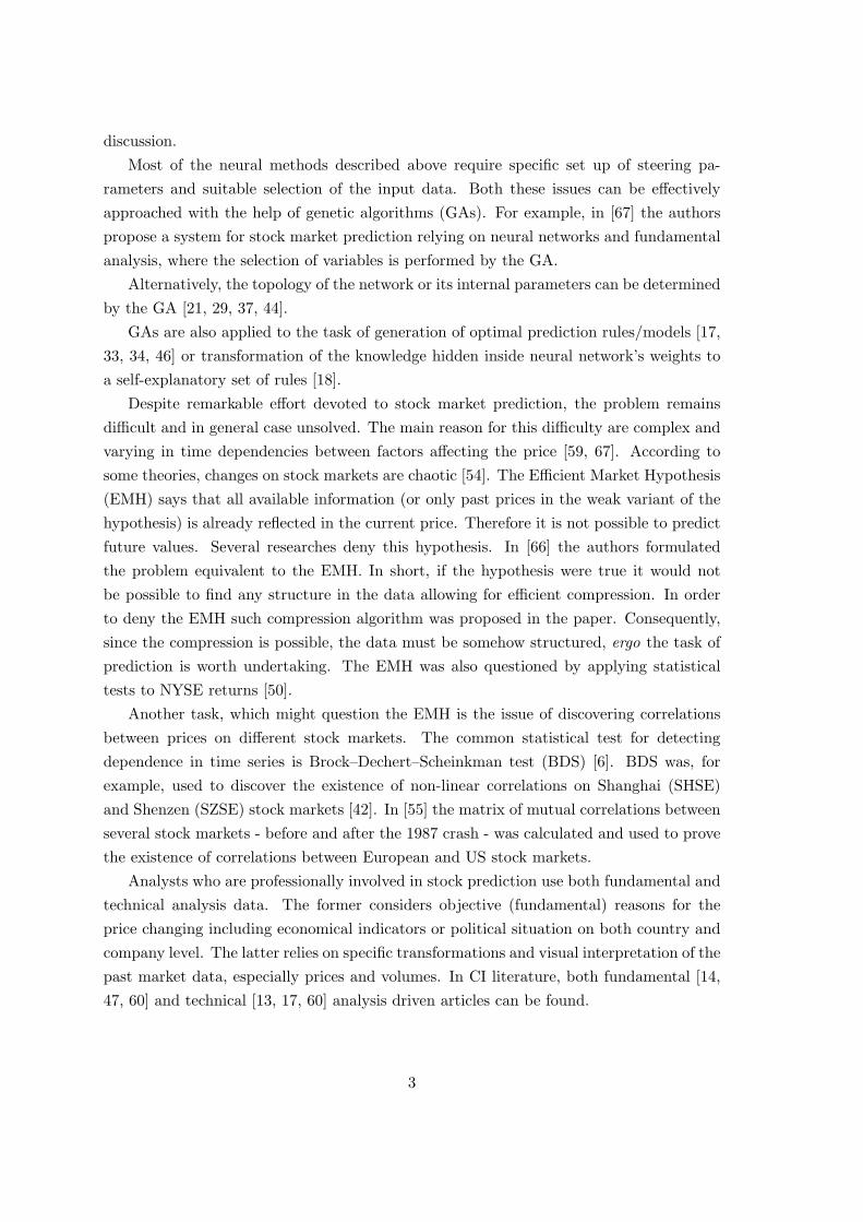
In order to examine the properties of Model 3 in more detail two specific periods were
cut out from Fig. 14. The first one from day 28th to day 59th represents an upward trend
(see Fig. 16) and the other one between days 14 and 28 - a downward trend (Fig. 17).
An examination of the two above periods shows that prediction based on neuro-genetic
model works well during both uptrend and downtrend. When the index value goes down
our model is able to gain some extra money on local changes of the trend. At the same
27

Figure 15: Differences in returns between proposed system and comparative models. Pos-itive values indicate higher profit of the proposed system.
time Model 4 based on MACD signals is comparable, but slightly worse. MACD generated
signal buy on the first day and signal sell on the next day. No more signals were generated,
so the model was not active during the downtrend. In case of an increasing trend our
algorithm is still able to utilize local changes of an index rate. Thanks to consequently
rising index value the final result of Model 1 (which makes profit by definition in case of
upward trend) is only slightly worse. Contrary to downtrend case, Model 4 places the
worst in uptrend situation. Model 2 places the third in both figures.
6.2 Repeatability of results
In order to verify whether the proposed method leads to repeatable results, the basic
experiment concerning Model 3 with Exp. 4 settings was repeated several times with the
same algorithm settings and for the same time period. The results are presented in Table 4.
The outcomes of returns ranged from 3.41% to 9.31% (with the average of 5.76%), which
is a promising result compared to loses of Models 1, 2 and 4 presented in Table 3. An
important feature of the repeated experiments was pairwise similarity between the variable
sets selected by GA in individual runs. In detailed analysis performed for the first three
runs, the variables chosen at each step (out of 20) were compared. At each step, the
number of variables common for all three runs and common for any two out of three ones
28
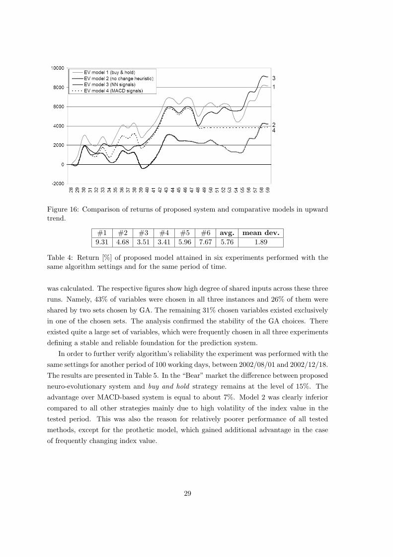
Figure 16: Comparison of returns of proposed system and comparative models in upwardtrend.
#1 #2 #3 #4 #5 #6 avg. mean dev.
9.31 4.68 3.51 3.41 5.96 7.67 5.76 1.89
Table 4: Return [%] of proposed model attained in six experiments performed with thesame algorithm settings and for the same period of time.
was calculated. The respective figures show high degree of shared inputs across these three
runs. Namely, 43% of variables were chosen in all three instances and 26% of them were
shared by two sets chosen by GA. The remaining 31% chosen variables existed exclusively
in one of the chosen sets. The analysis confirmed the stability of the GA choices. There
existed quite a large set of variables, which were frequently chosen in all three experiments
defining a stable and reliable foundation for the prediction system.
In order to further verify algorithm’s reliability the experiment was performed with the
same settings for another period of 100 working days, between 2002/08/01 and 2002/12/18.
The results are presented in Table 5. In the “Bear” market the difference between proposed
neuro-evolutionary system and buy and hold strategy remains at the level of 15%. The
advantage over MACD-based system is equal to about 7%. Model 2 was clearly inferior
compared to all other strategies mainly due to high volatility of the index value in the
tested period. This was also the reason for relatively poorer performance of all tested
methods, except for the prothetic model, which gained additional advantage in the case
of frequently changing index value.
29

Figure 17: Comparison of returns of proposed system and comparative models in down-ward trend.
Model Return [%]
Model 1 -15.21
Model 2 -26.45
Model 3 0.19
Model 4 -7.39
Table 5: Returns of tested models attained in another time period lasting from 2002/08/01to 2002/12/18.
6.3 Stability of results
Additional experiment was performed to examine the stability of attained results. The
test period of 100 trading days was shifted by 5, 10, 15, and 20 days. The other experiment
conditions remained unchanged. The results obtained for neighboring 100-day time periods
(overlapped in 95%) were compared. As can be seen from Table 6 the maximum absolute
change of the final budget between subsequent 5-day shifts equals 2.08%. In other words,
during the tested periods, the gain of the neuro-genetic system varied between 8214 and
10468 units, which is between 8.21% and 10.47% of the initial budget. The percentage
difference between investment periods shifted by 20 days (a−ea 100%) is less than 0.02%.
Relatively small changes of returns in subsequent periods support the claim that the
results of the neuro-genetic system are stable and repeatable.
30

Time shift Final budget [units] Change [%]
0 (original experiment) a = 109 315.36 -
5 days b = 110 076.75 a−ba 100 = −0.70
10 days c = 108 214.21 b−cb 100 = +1.69
15 days d = 110 467.53 c−dc 100 = −2.08
20 days e = 109 297.39 d−ed 100 = +1.06
Table 6: Returns of neuro-genetic system in subsequent time-windows.
6.4 “Rationality” of GA-based variable selection
Along with numerical tests an analysis of variables chosen in subsequent steps was per-
formed. The hypothesis to be verified is that variables are repeated in several subsequent
steps according to their importance in the current situation. In other words, it is claimed
that variables are not randomly chosen but selected by the algorithm with some visible
sense.
The expected ”rationality” of GA-based choices is manifested by its consistency with
the general rules used by professional stock market traders. In particular, the following
four observations come out from the analysis of the variable sets selected by the GA in
subsequent steps: (1) the frequent choice of variables from the target market compared to
the other sources of variables; (2) preference of stock-related variables over the exchange-
rates; (3) preference of NYSE variables over the TSE ones; and (4) different time of
usability of particular oscillators. As mentioned above all these four features are pertinent
factors of the human way of trading and they all reflect common knowledge in the field
(e.g. much higher influence of US stock market than the Japanese one on the European
markets).
The above four claims and discussed in the remainder of this section. First, the re-
sume of the variables’ selection during the first three steps (out of 20 ones performed) is
presented. For each step the variable percentage closing value was also present since it was
forced by the GA implementation. This variable is not listed. Variables from the target
GSE stock market were calculated for any of the t− n last days, for n = 0, ..., 5.
The note “en”, where 1 ≤ n ≤ 20 denotes that this particular variable also appeared (in
exactly the same form) in step number n. The prefix s preceding the step number means
that the meaning of the respective variable (in current step and in step n) is practically
the same (e.g. the average value of the past 20 days is nearly the same for today and
yesterday). For example,
• DAX[t] > IMPET10 [s4, s7, s8, s13, s15, s17, e20]
in the first line of Step 1 below means that the IMPET of the last 10 days (today’s
closing value of DAX (i.e. DAX[t]) minus closing value od DAX 10 days before) was chosen
31

as the first input variable and this same variable was also chosen in exactly the same form
in Step 20 and in a very similar form (e.g. calculated for days [t-1] and [t-11]) in Steps
4, 7, 8, 13, 15, 17. CHANGEn(%) denotes n days change in per cent of the respective
value, for n = 5, 10, 20. CHANGE O(C) denotes a change in opening(closing) value of
particular variable.
Step 1:
• DAX[t] > IMPET10 [s4, s7, s8, s13, s15, s17, e20];
• DAX[t] > SO [e3, e4, e6, e7];
• DAX[t] > IMPET20 [s4, s7, s8, e13, s15, s17, s20];
• DAX[t-2] > CHANGE10(%) [s2, s4, s5, s6, s8, s10, s11, s12, s14, s15, s16, s18, s19, s20];
• DAX[t-5] > MOV AVG10 [s4, s6, s7, s11];
• DAX[t] > CHANGE5(%) [s2, s4, s5, s6, s8, s10, s11, s12, s14, e15, s16, s18, s19, s20];
• DAX[t] > DAY NO [e2, s5, e8, e9, e10, s11, e12, e13];
• DAX[t-2] > CHANGE20(%) [s2, s4, s5, s6, s8, e10, s11, s12, s14, s15, s16, s18, s19, s20];
Step 2:
• DAX[t-1] > CHANGE5(%) [s1, s4, s5, s6, s8, s10, s11, s12, s14, s15, s16, s18, s19, s20];
• DAX[t] > DAY NO [e1, s5, e8, e9, e10, s11, e12, e13];
• DAX[t-4] > CHANGE10(%) [s1, s4, s5, s6, e8, s10, e11, s12, s14, s15, s16, s18, s19, s20];
• DAX[t-1] > CHANGE10(%) [s1, s4, s5, s6, s8, s10, s11, s12, s14, s15, s16, s18, s19, s20];
• DAX[t-1] > CHANGE C(%) [s1, s3, s4, s5, s6, s7, s8, s9, s11, s12, s13, s14, s15, s16, s17,
s18, s19, s20];
• DJIA[t] > CHANGE C(%) [e3, e4, e8, e9, e12, e14, e16, e17, e19];
• DAX[t] > CHANGE5(%) [s1, s4, s5, s6, s8, s10, s11, s12, s14, e15, s16, s18, s19, s20];
• DAX[t] > PATTERN SHIFTED [s9, s10];
• DAX[t] > CHANGE O(%) [s1, s3, s4, s5, s6, s7, s8, s9, s11, s12, s13, s14, s15, s16, e17, s18,
s19, s20];
Step 3:
• DAX[t] > SO [e1, e4, e6, e7];
• USD/JPY[t] > CHANGE C(%) [e7, e9, e10, e20];
• DJIA[t] > CHANGE C(%) [e2, e4, e8, e9, e12, e14, e16, e17, e19];
32

In the remaining steps 4-20 the situation was analogous: the majority of chosen
variables came from the target market (GSE), but aside from these variables there were
also variables from the other sources (NYSE, TSE and exchange rates). The frequency
of choosing variables from various sources is presented in Table 7. These figures should
be compared with the overall availability of variables from particular sources. Table 8
presents a comparison of percentage use of variables from particular sources across all 20
steps and the percentage availability of them in the whole pool of variables used by the
GA. These two distributions are clearly different. Except for the data from GSE, which
covers the majority of available variables, each of the remaining four sources provides one
variable, hence having the same probability of occurrence (1, 35%). The GA visibly prefers
the data from American NYSE (DJIA index closing value) over the one from Japanese
TSE (NIKKEI index closing value). Such preference is in line with investors’ knowledge,
who consider the US stock market as being more indicative for the changes on European
stock markets than the Japanese one. This observation is additionally validated by the
correlation plot presented in Fig. 4.
Another conclusion from Table 8 is that stock related variables are generally more
important than exchange rates. This observation is again in line with the knowledge
possessed by investors and stock analysts and confirms conclusions presented in the lit-
erature [55]. An order of frequency of the use of variables from different stock markets
generally agrees with preliminary analysis of correlation between variables.
Origin of variable Occurrence in steps
GSE all 20 steps
NYSE 10 steps
TSE 6 steps
USD/JPY 5 steps
EUR/USD 3 steps
Table 7: Frequency of choosing variables during the experiment.
Origin of variable Occurrence in results [%] Availability for GA [%]
GSE 84.11% 94.60%
NYSE 6.62% 1.35%
TSE 3.97% 1.35%
USD/JPY 3.31% 1.35%
EUR/USD 1.99% 1.35%
Table 8: Percentage use of variables.
It is worth to underline that any variable chosen in any step is also present in at least a
few more steps either directly or as a similar (s.) type of variable. Some of the variables are
being chosen (survive) in a few steps in a row. Both the above observations suggest that
33

the selection of input variables performed by the neuro-genetic system in not accidental
and some variables are visibly preferred over the other ones. Variables are chosen according
to their impact on networks effectiveness. The results suggest that for a given period of
time (5 trading days) selected variables provide relevant information concerning current
situation on a stock market, which allows making a high quality prediction.
An interesting observation is related to frequent appearance of oscillators among chosen
input variables. These oscillators are usually preferred for one or at most two consecutive
time steps and then replaced by another ones. This is in accordance with stock market
analysts’ judgement who use particular oscillators only for a limited period of time, since
changes on stock market require adequate adaptation of these instruments. The appear-
ance of oscillators in different steps of experiment is presented in Table 9. The most
frequently used ones are Impet (8 times), Stochastic, and MACD (5 times each). These
figures prove the usefulness of the information represented by oscillators in stock market
index prediction. Recall that one of the comparative models (Model 4) is based exclusively
on signals generated by the MACD oscillator.
Step 1 - Stochastic and Impet Step 11 - ROCStep 2 - no oscillator chosen Step 12 - WilliamsStep 3 - Stochastic Step 13 - ImpetStep 4 - Stochastic and Impet Step 14 - MACDStep 5 - RSI, ROC and MACD Step 15 - Impet and WilliamsStep 6 - Stochastic and ROC Step 16 - 2 AVG’sStep 7 - Stochastic, Impet, Williams and MACD Step 17 - ImpetStep 8 - Impet and 2 AVG’s Step 18 - no oscillator chosenStep 9 - MACD Step 19 - 2 AVG’s and MACDStep 10 - no oscillator chosen Step 20 - Impet
Table 9: Oscillators chosen in subsequent steps.
Another key observation coming out from manual data analysis is high consistency of
the variable selection process between experiments. As we have presented in Section 6.2
the main experiment was repeated 6 times for the same period of time and with the same
parameters settings (though each time with random selection of the initial population).
One of the crucial findings was the observation that if for any of the 6 experiment in any
given step n, 1 ≤ n ≤ 20 all of the selected values were connected to DAX index, then in
all the remaining experiments all selected values in step n were also connected with DAX
(either in the form of an exact repetition or as a similar value - as described above in this
section). Only sporadically (in 4 steps out of 20 in 1 out of 6 runs) an additional variable
appeared, which was not connected with DAX. Certainly, the frequency of choosing DAX
variables is not surprising considering the fact that they constitute 81% of all variables,
but what is surprising is the consistency of the choices in the same steps across various
34

runs/experiments. For example, in Step 3, in all experiments the selected variable sets
include index DJIA and the currency exchange rates (which are very uncommon among
the whole pool of input variables). This observation clearly suggests that the choice made
by the GA is governed by some underlying “logic”.
The consistency of the variable selection process, for the sake of clarity of the figure
illustrated across the first three experimental runs only, is presented in Fig. 18.
Figure 18: Consistency of variable selection across three independent experiments.
Additional analysis of “rationality” of the GA-based variable choices was performed
by modifying the experiment’s scenario in a way that the network proposed by GA was
not applied to the immediate time window prediction, but for the next one (shifted one
step forward). This so-called shifted neuro-genetic system (see Fig. 19) was compared
with the previously described one (cf. Fig. 9). The results are presented in Table 10
and Fig. 20. The original neuro-genetic system outperforms its shifted version by more
than 10%. The results show that using the same choice of input variables and the same
network architecture (although retrained on the new, current data) for the next 5 days is
less effective than applying a new choice of inputs and new neural architecture (chosen by
the GA), which are better fitted to the actual situation on the market. On the other hand
the shifted neuro-genetic system’s profit is higher than the one of buy and hold strategy,
which suggests that the network chosen in the previous step of GA (after retraining on
new, available data) still yields reasonable results.
The difference between earned values of the original and the shifted systems during the
35

Figure 19: A modified scenario for experiment with network used for the shifted 5-daywindow.
Model Return [%]
Buy and hold −4.99
Shifted neuro-genetic −2.26
“Original” neuro-genetic 8.31
Table 10: Return generated by buy and hold, “original” neuro-genetic and shifted neuro-genetic models. Please note, that the difference in results achieved by the “original”neuro-genetic model reported in Tables 3 and 10 is caused by a shorter investment periodin the latter case, i.e. 100 vs. 95 trading days, resp. The same note applies to the buyand hold strategy.
test phase is presented in Fig. 21. Every increase of the value in the plot means that the
original system gets higher return than the shifted one, and vice versa. There are two time
periods, during which the original system visibly increases its profit, i.e. days 13–20 with
rapid growth and days 33–69 with moderately increasing trend though taking place over
a long time period. On the other hand short periods with the superiority of the shifted
system are also observable, e.g. days 29–33, 85–95 and day 81, however the magnitude of
profit’s decrease is comparably lower.
7 Summary and conclusions
A hybrid neuro-genetic method of prediction with application to financial task, which is
prediction of the closing value of DAX - the German Stock Exchange index, is presented
and examined in the paper. Assuming the flow of information between different stock
markets and their mutual relations the proposed system uses data from five different
sources: three stock markets and two exchange rates. The analysis of the use of variables
confirms the hypothesis of a correlation between different stock markets. The frequency of
choosing variables from NYSE (TSE) markets was respectively 5(3) times higher than their
36

Figure 20: Changes of return of between buy and hold, original neuro-genetic and shiftedneuro-genetic models during 19 steps.
percentage availability in the pool of variables. These variables were also more preferable
than the exchange rates.
Due to changing in time dependencies between variables describing financial markets
(indices, oscillators, exchange rates, etc.) and assuming that the usefulness of any variable
is limited in time, the proposed approach relies on applying the GA to frequent input data
selection (among the predefined pool of variables from the above mentioned five sources).
The standard GA procedure is enhanced by adding a new type of crossover operator
and a mechanism that controls the range of chromosomes’ sizes. Furthermore, the chro-
mosomes are categorized as being either alive (i.e. the neural net architectures coded by
them are able to learn) or dead (in the opposite case). Based on the ratio between alive
and dead chromosomes the probabilities of genetic operators are changing accordingly in
order to get rid of useless, non-alive chromosomes.
Another modification to the “canonical” GA implementation is introduction of the
three categories of variables: best chromosome, often selected and common with different
probabilities of selection for crossover and mutation. Performed numerical tests confirmed
the usefulness of the above variability of the input data, which accelerated the convergence
of the GA without having a negative impact on the quality of results.
All of the above triggers and control mechanisms are based on predefined rules and
therefore the prediction system once set-up and started works subsequently without human
37

Figure 21: Difference in return between original neuro-genetic and shifted neuro-geneticmodels.
intervention or prompting.
During the test phase, the proposed method of prediction attained between 3.4% and
9.3% of a profit compared to the loss of 3.6% or more yielded by the other tested methods
(excluding the omnipotent, prophetic model). Moreover, the proposed system was able to
keep up with the prophetic (locally optimal) model in several subperiods of testing days.
Comparable results were also attained for another 100-day period in the year 2002, when
neuro-genetic system outperformed Models 1, 2 and 4 by more than 7.5%. The system
works well in both upward and downward trend situations on the stock market.
Except for encouraging numerical results, the very important aspect of this research
was the “qualitative behavior” of the proposed system, that is its ability to choose the
efficient set of input variables and neural net’s architecture adequately defining the current
situation on the predicted stock market. Consequently the “rationality” of GA’a choices
was examined. First of all, in all steps of the test phase various similarities between
choices of input variables in subsequent steps were discovered. Since the exactness of
any financial indicator (oscillator, signal, etc.) varies in time, having some indicators
shared between subsequent steps is an expected and promising feature. Certainly, in each
step a number of new variables is also expected to appear and replace the “used” and not
adequate ones. Additionally, the experiment with using the neural architecture and the set
of input variables chosen in the previous step for prediction shifted one step forward (after
retraining on the latest available input data) output noticeably worse results compared
38

to the case of using these networks with associated input sets for the related (current)
prediction steps.
The results confirm the hypothesis about changing in time dependencies between vari-
ables. The frequency analysis of choosing variables from three different stock markets to
the current input set proved the hypothesis that stock markets are related and that the
influence of NYSE on the GSE (generally, on European stock markets) is prevailing the
one of Japanese TSE. Although this observation is well-known for any professional trader,
discovering and considering such relation by the prediction system itself is an indication
of system’s reliability and efficiency.
Numerical results and the above qualitative observations support a conclusion that the
evolutionary-based input variables selection and the choice of network’s architecture are
reasonable and the proposed hybrid, neuro-genetic prediction system works efficiently.
8 Directions for future research
The main future goal is the extension of the system allowing for generation of the wait
signal not only in the case of zero-change forecast, but also in case none of the two other
possible decisions (buy, sell) is convincing enough.
We also plan to improve the settings of parameters of the GA and the learning process
of the final neural network, which should result in overall better prediction abilities.
We also think of applying the method to prediction of a particular stock instead of an
index.
Moreover, we plan to do comparative analysis of our approach and the one presented
in [43] where, similarly to our work, GA was applied to input variable pre-selection. In
order to make this comparison fair both methods would be modified with respect to the
length of the applicability period of GA-based variable set (which is equal to one year
in [43]) as well as applied on the common data sets.
Finally, the use of dynamic correlations between variables in order to guide the selection
process implemented by the GA seems to be a potentially promising direction. We plan
to investigate this research avenue, however, the results of initial tests indicated that the
effectiveness of the neural prediction system (with no use of GA), which input choice was
based solely on correlation between variables yielded inferior results compared to using
full neuro-genetic procedure. This observation, if proven in extensive tests, would further
confirm the strength and usefulness of genetic algorithm based variable selection.
39

Acknowledgment
Jacek Mandziuk was supported in this work by the Warsaw University of Technology grant
no. 504G 1120 0008 000.
Appendix 1. A pseudocode of the proposed system
main()
{rawDataSet = LoadData(file);
dataSet = CreateDataSet(rawDataSet);
/* Further description of algorithm is limited to main experiment scenario only
(input variables selected by GA). Functionalities of selection by autocorrelation or
manual selection or expert voting are not described. */
PerformPredictionsForExperiment(dataSet);
/* It runs GA for variables selection, performs NN learning and testing.*/
AddPredictionsForComparison(dataSet);
/* It calculates decisions buy or sell using alternative methods. This is not presented
in details.*/
RunGame(dataSet);
/* It calculates final result of the experiment based on saved decisions. This
is not presented in details.*/
}
rawDataSet: LoadData(file)
{rawData = LoadDataFromFile(file);
rawDataSet = CreateRawDataSet(rawData);
AddSimpleTrasformations(rawDataSet);
AddOscillators(rawDataSet);
AddOscillatorsSignals(rawDataSet);
CleanRawData(rawDataSet);
return rawDataSet;
}
dataSet: CreateDataSet(rawDataSet)
{dataSet = ConvertRawDataSet(RawDataSet);
CleanDataSet(dataSet);
40

CalculateAttributes(dataSet); /* min/max attributes */
return dataSet;
}
PerformPredictionsForExperiment(dataSet)
{SetUpLearningParamters(context);
for (each step)
/* If experiment is without repeating learning after each step it is understood
as one-step experiment.*/
{/* Select variables according to experiment set up.*/
if (context.selectVariablesByGA = true) SelectVariablesByGA(dataSet);
if (context.selectVariablesByAC = true) SelectVariablesByAC(dataSet);
if (context.selectVariablesManually = true) SelectVariablesManually(dataSet);
dataSetsForLearning = SetUpDataSetsForLearning(dataSet);
/* Prepare learning / test / validation sets.*/
for (each day within step)
{if (context.expertVoting = true and context.selectVariablesByGA = true)
{for (each chromosome in context.listOfBestChromosomes[])
{network = CreateNetworkBasedOnSelectedVariables(chromosome);
network.LearnBP(dataSetsForLearning);
RunPrediction(network, dataSetForLearning);
/* Number of predictions is generated. Finally voting will point out buy or sell
signal.*/
}}else
{network = CreateNetworkBasedOnSelectedVariables();
network.LearnBP(dataSetsForLearning);
RunPrediction(network, dataSetForLearning); /* One prediction is generated.*/
}}}}
inputVariables: SelectVariablesByGA(dataSet)
41
{SetUpRunningParameters(context);
/* Context means all external variables set up in application.*/
if (initialTruncateOfVariables) SelectMainVariablesAvailableForGA();
else SelectAllVariablesAvailableForGA();
if (initialPreselectionByAutocorrelation) SelectVariablesByAC(dataSet);
/* This is not further described.*/
SetUpGeneralParametersOfGA(context, dataSet);
/* Static parameters like size of population are set.*/
probabilityOfMutation = SetUpInitialParametersOfGA(parametersSet1);
/* There are two sets of parameters for GA: initial and one dedicated for last iterations
of GA. In this implementation this set consists of mutation probability only.*/
SetUpInitialPopulation(context, dataSet);
SetUpNeuralNetworksSetsForGAPopulation(context, dataSet);
/* Each chromosome is represented by set of NNs.*/
poolOfThreads = SetUpStructuresForParallelComputations(context);
SetUpStructuresForGA(dataSet);
for (iteration <= context.iterationLimit)
{if (iteration = = thresholdForParamtersChange)
probabilityOfMutation = SetUpInitialParametersOfGA(parametersSet2);
/* Calculating adaptation values for each chromosome if it is not calculated (initial
population or after mutation).*/
SetUpSteeringParametersForLearning(parents = true);
for (each thread)
{poolOfThreads(thread) = new Thread ParallelLearningNN();
poolOfThreads(thread).start();
}WaitForAllThreadsDone(poolOfThreads);
if (iteration > 1)
/* There are no children in first iteration.*/
{SetUpSteeringParametersForLearning(children = true);
for (each thread)
{poolOfThreads(thread) = new Thread ParallelLearningNN();
poolOfThreads(thread).start();
}WaitForAllThreadsDone(poolOfThreads);
ChangeParentsToChildren();
/* This function checks if parent is indicated to be replaced according to results
of ranking and does it only if adaptation value of children is higher than parent.*/
42

}/* Mutation of population */
for (each chromosome in population)
{if (chromosome is not bestChromosome or context.mutationDoesNotAffectBestChromosome
= false)
{chromosome.Mutate(allAlive, sizeMutation, probabilityOfMutation);
/* Mutation has different probability if population is young with many ’dead’ chromosomes
than mature population. Situation when mutation of size is also considered.*/
}}DrawParsForRanking();
/* Randomly matches chromosomes into pairs which will compete to be parents.*/
for (each two pars : par1, par2)
{winningPar = PointParWhichWillBeParents();
/* This is done according to adaptation values.*/
if (winningPar = par1) loosingPar = par2; else loosingPar = par1;
CreateChildren(context.typeOfCrossing, takeCodeFrom = winningPar, markForReplacement
= loosingPar);
/* It does crossing of different types: by dividing point or by product of parents.*/
}bestChromosome = PointBestChromosome(bestChromosome);
/* Find current best chromosome and change global best one if it is better adapted.*/
}if (context.extraImprovement = true)
/* Create new population of mutated best chromosome*/
{SetUpInitialPopulationOfMutatedBestChromosome();
/* This population will be created by chromosomes that differs in one variable from
best one.*/
for (iteration <= bestChromosome.size)
/* Every variable of best chromosome will be changed to new one.*/
{for (each indexOfVariable)
/* Every not used variable will be placed instead of changed variable of best chromosome.*/
{if (indexOfVariable in bestChromosome) next;
/* In case of duplication of variables within single chromosome omit this variable.*/
mutatedBestChromosome=bestChromosome;
mutatedBestChromosome.variable[iteration] = indexOfVariable;
AddChromosomeToPopulationOfMutatedBestChromosome(mutatedBestChromosome);
43

}}/* Calculate adaptation of population of mutated best chromosome.*/
SetUpSteeringParametersForLearning(extraImprovement = true);
for (each thread)
{poolOfThreads(thread) = new Thread ParallelLearningNN();
poolOfThreads(thread).start();
}WaitForAllThreadsDone(poolOfThreads);
bestChromosome = PointBestChromosome(bestChromosome);
/* Check if there is new global best chromosome in population of mutated best chromosome.*/
}context.listOfBestChromosomes[] = FindBestChromosomesInFinalPopulation(context.numberOfExperts);
/* There is scenario in which decision is based not on one network answer but set
of best networks.*/
SelectVariables(bestChromosome);
return inputVariables;
}
chromosome: Mutate(allAlive, sizeMutation, probabilityOfMutation)
{if (allAlive = true)
chromosome.DoMutationOfVariables(probabilityOfMutationIfAllAlive(probabilityOfMutation));
else
chromosome.DoMutationOfVariables(probabilityOfMutationIfNotAllAlive(probabilityOfMutation));
/* Probability of mutation is different in early iterations when many chromosomes
are not alive which means that coded set of variables is not sufficient for successful
learning.*/
if (sizeMutation = true) chromosome.DoMutationOfSize();
chromosome.RemoveDuplicatedVaraibles();
return chromosome;
}
ParallelLearningNN()
{Monitor.Enter();
if (CheckExitCondition() = true) return;
SetUpLocalThreadParamters(context);
Monitor.Exit();
for (each chromosome)
44

{dataSetsForLearning = SetUpDataSetsForLearning();
/* Prepare learning / test sets specific for chromosome.*/
for (each network assigned to chromosome)
/* Adaptation is calculated according to results from number of networks.*/
{network.LearnBP(dataSetsForLearning); /* BP learning algorithm.*/
mse[network] = network.Test(dataSetsForLearning);
/* Simple test of NN response.*/
}if (context.fitnessByAverage = true) chromosome.SetUpAdaptationByAverage(mse[network]);
if (context.fitnessByMinimum = true) chromosome.SetUpAdaptationByMinimum(mse[network]);
}}
45

References
[1] Y. Baram. Partial classification: The benefit of deferred decision. IEEE Transactions
on Pattern Analysis and Machine Intelligence, 20(8):769–776, 1998.
[2] N. Bauerle and U. Rieder. Technical notes and correspondence: Portfolio optimiza-
tion with markov-modulated stock prices and interest rates. IEEE Transactions on
Automatic Control, 49(3):442–447, 2004.
[3] Y. Bengio and P. Frasconi. Input-output HMM’s for sequence processing. IEEE
Transactions on Neural Networks, 7(5):1231–1249, September 1996.
[4] Y. Bengio, V.-P. Lauzon, and R. Ducharme. Experiments on the application of
IOHMMs to model financial returns series. IEEE Transactions on Neural Networks,
12(1):113–123, 2001.
[5] F. Black and M. Scholes. The pricing of options and corporate liabilities. J. Political
Economy, 81:637–654, 1973.
[6] W. A. Brock, W. D. Dechert, and J. A. Scheinkman. A test for independence based
on the correlation integral. Technical Report. University of Wisconsin-Madison, 1986.
[7] J. Brodka. Private communication, 2006.
[8] L. Cao and F. Tay. Support Vector Machine with adaptive parameters in financial
time series forecasting. IEEE Transactions on Neural Networks, 14(6):1506–1518,
2003.
[9] L. J. Cao, K. S. Chua, W. K. Chong, H. P. Lee, and Q. M. Gu. A comparison
of PCA, KPCA and ICA for dimensionality reduction in Support Vector Machine.
Neurocomputing, 55:321–336, 2003.
[10] E. Capobianco. Independent component analysis and resolution pursuit with wavelet
and cosine packets. Neurocomputing, 48:779–806, 2002.
[11] T. Chenoweth and Z. Obradovic. A multi-component nonlinear prediction system for
the S&P 500 index. Neurocomputing, 10:275–290, 1996.
[12] Y. Cheung and L. Xu. Independent component ordering in ica time series analysis.
Neurocomputing, 41:145–152, 2001.
[13] F.-L. Chung, T.-C. Fu, V. Ng, and R. Luk. An evolutionary approach to pattern-
based time series segmentation. IEEE Transactions on Evolutionary Computation,
8(5):471–489, 2004.
46
[14] H. Chung and J.-B. Kim. A structured financial statement analysis and the direct
prediction of stock prices in Korea. Asia-Pacific Financial Markets, 8:87–117, 2001.
[15] T. Cover. An algorithm for maximizing expected log investment return. IEEE Trans-
actions on Information Theory, 30(2):369–373, 1984.
[16] G. Deco, R. Neuneier, and B. Schurmann. Non-parametric data selection for neural
learning in non-stationary time series. Neural Networks, 10(3):401–407, 1997.
[17] M. Dempster, T. Payne, Y. Romahi, and G. Thompson. Computational learning tech-
niques for intraday FX trading using popular technical indicators. IEEE Transactions
on Neural Networks, 12(4):744–754, 2001.
[18] W. Duch, R. Setiono, and J. Zurada. Computational intelligence methods for rule-
based data understanding. Proceedings of the IEEE, 92:771–805, 2004.
[19] J. L. Elman. Finding structure in time. Cognitive Science, 14:179–211, 1990.
[20] S. E. Fahlman and C. Lebiere. The cascade-correlation learning architecture. In David
Touretzky, editor, Advances in Nueral Information Processing Systems 2, pages 524–
532, San Mateo, CA, USA, 1990. Morgan Kaufmann.
[21] J. Fieldsend and S. Singh. Pareto evolutionary neural networks. IEEE Transactions
on Neural Networks, 16(2):338–354, 2005.
[22] Norbert Fiess and Ronald MacDonald. Technical analysis in the foreign exchange
market: A cointegration-based approach. Multinational Finance Journal, 3(3):147–
172, 1999.
[23] V. Gavrishchaka and S. Ganguli. Volatility forecasting from multiscale and high-
dimensional market data. Neurocomputing, 55:285–305, 2003.
[24] R. Gencay and M. Qi. Pricing and hedging derivative securities with neural networks:
Bayesian regularization, early stopping, and bagging. IEEE Transactions on Neural
Networks, 12(4):726–734, 2001.
[25] T. Gestel, J. Suykens, D.-E. Baestaens, A. Lambrechts, G. Lanckriet, B. Vandaele,
B. De Moor, and J. Vandewalle. Financial time series prediction using Least Squares
Support Vector Machnies within the evidence framework. IEEE Transactions on
Neural Networks, 12(4):809–820, 2001.
[26] T. H. Hann and E. Steurer. Much ado about nothing? exchange rate forecasting:
Neural networks vs. linear models using monthly and weekly data. Neurocomputing,
10:323–339, 1996.
47

[27] J. V. Hansen and R. D. Nelson. Data mining of time series using stacked generalizers.
Neurocomputing, 43:173–184, 2002.
[28] B. Hassibi and D. Stork. Secong order derivatives for network pruning: Optimal Brain
Surgeon. In David Touretzky, editor, Advances in Nueral Information Processing
Systems 5, pages 164–171, San Mateo, CA, USA, 1993. Morgan Kaufmann.
[29] S. Hayward. The role of heterogeneous agents past and forward time horizons in
formulating computational models. Computational Economics, 25:25–40, 2005.
[30] Po-Hsuan Hsu and Chung-Ming Kuan. Reexamining the profitability of technical
analysis with data snooping check. Journal of Financial Econometrics, 3(4):606–628,
2005.
[31] M. Jaruszewicz and J. Mandziuk. One day prediction of NIKKEI index considering
information from other stock markets. L. Rutkowski et al. (Ed.), ICAISC, Lect. Notes
in Art. Int., 3070:1130–1135, 2004.
[32] M. Jaruszewicz and J. Mandziuk. Neuro-genetic system for DAX index prediction.
A. Cared and L. Rutkowski and R. Tadeusiewicz and J. Zurada (Ed.), Artificial In-
telligence and Soft Computing, pages 42–49, 2006.
[33] G. John, P. Miller, and R. Kerber. Stock selection using rule induction. IEEE Expert,
pages 52–58, 1996.
[34] M. Kaboudan. Genetic programming prediction of stock prices. Computational Eco-
nomics, 16:207–236, 2000.
[35] S. Kamitsuji and R. Shibata. Effectiveness of stochastic neural network for prediction
of fall or rise of topix. Asia-Pacific Financial Markets, 10:187–204, 2003.
[36] A. Kim, Ch. Shelton, and T. Poggio. Modeling stock order flows and learning market-
making from data. MIT, 2002.
[37] K. Kim and W. Lee. Stock market prediction using artificial neural networks with
optimal feature transformation. Neural Computing & Applications, 13:255–260, 2004.
[38] S. Kim. Time-delay recurrent neural network for temporal correlations and prediction.
Neurocomputing, 20:253–263, 1998.
[39] V. Kodogiannis and A. Lolis. Forecasting financial time series using neural network
and fuzzy system-based techniques. Neural Computing & Applications, 11:90–102,
2002.
48
[40] K. Kohara, Y. Fukuhara, and Y. Nakamura. Selective presentation learning for neural
network forecasting of stock market. Neural Computing & Applications, (4):143–148,
1996.
[41] N. Kohzadi, M. S. Boyd, B. Kermanshahi, and I. Kaastra. A comparison of artificial
neural network and time series models for forecasting commodity prices. Neurocom-
puting, 10:169–181, 1996.
[42] Patrick Kouk and Kun Chu. Using bds statistics to detect nonlinearity in time series.
Proceedings of the 53rd International Statistical Institute Conference in Seoul, 2001.
[43] Yung-Keun Kwon, Sung-Soon Choi, and Byung Ro Moon. Stock prediction based on
financial correlation. GECCO, pages 2061–2066, 2005.
[44] Yung-Keun Kwon and Byung Ro Moon. Nonlinear feature extraction using a neuro
genetic hybrid. GECCO, pages 2089–2096, 2005.
[45] T. L. Lai and S. P.-S. Wong. Valuation of American options via basis functions. IEEE
Transactions on Automatic Control, 49(3):374–385, 2004.
[46] M. Last, Y. Klein, and A. Kandel. Knowledge discovery in time series databases.
IEEE Transactions on Systems, 31(1):160–169, 2001.
[47] B. LeBaron. Empirical regularities from interacting long- and short-memory investors
in an agent-based stock market. IEEE Transactions on Evolutionary Computation,
5(5):442–455, 2001.
[48] Y. LeCun, J. Denker, and S. Solla. Optimal brain damage. In David Touretzky,
editor, Advances in Nueral Information Processing Systems 2, pages 598–605, San
Mateo, CA, USA, 1990. Morgan Kaufmann.
[49] R. Lee. iJADE Stock Advisor: An intelligent agent based stock prediction system
using hybrid RBF recurrent network. IEEE Transactions on Systems, 34(3):421–428,
2004.
[50] A. Lo and A. C. Mackinlay. Stock market prices do not follow random walks: Evidence
from a simple specification test. Rev. Financ. Stud., 1:41–66, 1988.
[51] M. Malliaris and L. Salchenberger. Using neural networks to forecast the S&P 100
implied volatility. Neurocomputing, 10:183–195, 1996.
[52] J. Mandziuk and M. Jaruszewicz. Neuro-evolutionary approach to stock market pre-
diction. In Proceedings of the International Joint Conference on Neural Networks
(IJCNN07), pages 2515–2520, Orlanodo, FL, USA, 2007. IEEE Press.
49
[53] J. Mandziuk and M. Jaruszewicz. “Dead” chromosomes and their elimination in the
neuro-genetic stock index prediction system. In International Conference on Neural
Information Processing (ICONIP’09), Lecture Notes in Computer Science, pages 601–
610, Bangkok, Thailand, 2009. Springer-Verlag.
[54] R. Mantegna and E. Stanley. An Introduction to Econophysics. Correlations and
Complexity in Finance. Cambridge University Press, 2000.
[55] I. Meric and G. Meric. Co-movements of european equity markets before and after
the 1987 crash. Multinational Finance Journal, 1(2):137–152, 1997.
[56] J. Moody and M. Saffell. Learning to trade via direct reinforcement. IEEE Transac-
tions on Neural Networks, 12(4):875–889, 2001.
[57] J. Murphy. Technical Analysis of the Financial Markets. New York Institiute of
Finance, 1999.
[58] W. O’Neil. Profit maximizing and price distortion minimizing codes for a channel
model of an asset market. IEEE Transactions on Information Theory, 41(6):2009–
2014, 1995.
[59] D. Ormoneit. A regularization approach to continuous learning with an application
to financial derivatives pricing. Neural Networks, (12):1405–1412, 1999.
[60] T. Poddig and H. Rehkegler. A “world” model of integrated financial markets using
artificial neural networks. Neurocomputing, 10:251–273, 1996.
[61] M. J. Pring. Technical Analysis explained: The Succesfull Investor’s Guide to Spot-
ting, Investment Trends and Turning Points. McGraw-Hill, 2002.
[62] The R Project for Statistical Computing. http://www.r-project.org, 2007.
[63] E. Saad, D. Prokhorov, and D. Wunsch. Comparative study of stock trend prediction
using time delay, recurrent and probabilistic neural networks. IEEE Transactions on
Neural Networks, 9(6):1456–1470, 1998.
[64] J. D. Schwager. Getting started in Technical Analysis. John Wiley & Sons, 1999.
[65] L. Shepp. A model for stock price fluctuations based on information. IEEE Transac-
tions on Information Theory, 48(6):1372–1378, 2002.
[66] A. Shmilovici, Y. Alon-Brimer, and S. Hauser. Using a stochastic complexity measure
to check the efficient market hypothesis. Computational Economics, 22:273–284, 2003.
50

[67] S. Thawornwong and D. Enke. The adaptive selection of financial and economic
variables for use with artificial neural networks. Neurocomputing, 56:205–232, 2004.
[68] P. Tino, Ch. Schittenkopf, and G. Dorffner. Financial volatility trading using recur-
rent neural networks. IEEE Transactions on Neural Networks, 12(4):865–874, 2001.
[69] V. Vapnik. The Nature of Statistical Learning Theory. Springer, 1995.
[70] V. Vapnik. Statistical Learning Theory. Wiley, 1998.
[71] H. Walk and S. Yakowitz. Iterative nonparametric estimation of a log-optimal port-
folio selection function. IEEE Transactions on Information Theory, 48(1):324–333,
2002.
[72] Wing-Keung Wong, Meher Manzur, and Boon-Kiat Chew. How rewarding is technical
analysis? evidence from singapore stock market. Technical Report wp0216, 2002.
[73] L. Xu. RBF nets, mixture experts, and Bayesian Ying-Yang learning. Neurocomput-
ing, 19:223–257, 1998.
[74] J. Yao and C. Tan. A case study on using neural networks to perform technical
forecasting of FOREX. Neurocomputing, 34:79–98, 2000.
51