Neural mechanism to simulate a scale-invariant future

Karthik H. Shankar, Inder Singh, and Marc W. Howard1

1Center for Memory and Brain, Initiative for the Physics and Mathematics of Neural Systems, Boston University

Predicting future events, and their order, is important for efficient planning. We propose a neuralmechanism to non-destructively translate the current state of memory into the future, so as toconstruct an ordered set of future predictions. This framework applies equally well to translationsin time or in one-dimensional position. In a two-layer memory network that encodes the Laplacetransform of the external input in real time, translation can be accomplished by modulating theweights between the layers. We propose that within each cycle of hippocampal theta oscillations, thememory state is swept through a range of translations to yield an ordered set of future predictions.We operationalize several neurobiological findings into phenomenological equations constrainingtranslation. Combined with constraints based on physical principles requiring scale-invariance andcoherence in translation across memory nodes, the proposition results in Weber-Fechner spacingfor the representation of both past (memory) and future (prediction) timelines. The resultingexpressions are consistent with findings from phase precession experiments in different regions ofthe hippocampus and reward systems in the ventral striatum. The model makes several experimentalpredictions that can be tested with existing technology.

I. INTRODUCTION

The brain encodes externally observed stimuli in realtime and represents information about the current spatiallocation and temporal history of recent events as activ-ity distributed over neural networks. Although we arephysically localized in space and time, it is often usefulfor us to make decisions based on non-local events, byanticipating events to occur at distant future and remotelocations. Indeed, optimal prediction is a major focus ofstudies of the physics of the brain [1–5]. Clearly, flexibleaccess to the current state of spatio-temporal memoryis crucial for the brain to successfully anticipate eventsthat might occur in the immediate next moment. In or-der to anticipate events that might occur in the futureafter a given time or at a given distance from the cur-rent location, the brain needs to simulate how the currentstate of spatio-temporal memory representation will havechanged after waiting for a given amount of time or af-ter moving through a given amount of distance. In thispaper, we propose that the brain can swiftly and non-destructively perform space/time-translation operationson the memory state so as to anticipate events to occurat various future moments and/or remote locations.

The rodent brain contains a rich and detailed repre-sentation of current spatial location and temporal his-tory. Some neurons–place cells–in the hippocampus firein circumscribed locations within an environment, re-ferred to as their place fields. Early work excluded con-founds based on visual [6] or olfactory cues [7], suggestingthat the activity of place cells is a consequence of someform of path integration mechanism guided by the ani-mal’s velocity. Other neurons in the hippocampus—timecells—fire during a circumscribed period of time withina delay interval [8–12]. By analogy to place cells, a set oftime cells represents the animal’s current temporal posi-tion relative to past events. Some researchers have longhypothesized a deep connection between the hippocam-

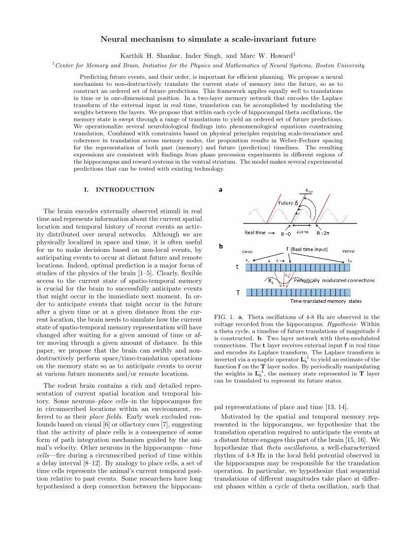
FIG. 1. a. Theta oscillations of 4-8 Hz are observed in thevoltage recorded from the hippocampus. Hypothesis: Withina theta cycle, a timeline of future translations of magnitude δis constructed. b. Two layer network with theta-modulatedconnections. The t layer receives external input f in real timeand encodes its Laplace transform. The Laplace transform isinverted via a synaptic operator L-1

k to yield an estimate of thefunction f on the T layer nodes. By periodically manipulatingthe weights in L-1

k , the memory state represented in T layercan be translated to represent its future states.

pal representations of place and time [13, 14].

Motivated by the spatial and temporal memory rep-resented in the hippocampus, we hypothesize that thetranslation operation required to anticipate the events ata distant future engages this part of the brain [15, 16]. Wehypothesize that theta oscillations, a well-characterizedrhythm of 4-8 Hz in the local field potential observed inthe hippocampus may be responsible for the translationoperation. In particular, we hypothesize that sequentialtranslations of different magnitudes take place at differ-ent phases within a cycle of theta oscillation, such that

2

a timeline of anticipated future events (or equivalentlya spaceline of anticipated events at distant locations) isswept out in a single cycle (fig. 1a).

Theta oscillations are prominently observed during pe-riods of navigation [17]. Critically, there is a systematicrelationship between the animal’s position within a neu-ron’s place field and the phase of the theta oscillation atwhich that neuron fires [18], known as phase precession.This suggests that the phase of firing of the place cellsconveys information about the anticipated future loca-tion of the animal. This provides a strong motivation forour hypothesis that the phase of theta oscillation wouldbe linked to the translation operation.

A. Overview

This paper develops a computational mechanism forthe translation operation of a spatial/temporal memoryrepresentation constructed from a two-layer neural net-work model [19], and links it to theta oscillations by im-posing certain constraints based on some neurophysiolog-ical observations and some physical principles we expectthe brain to satisfy. Since the focus here is to understandthe computational mechanism of a higher level cognitivephenomena, the imposed constraints and the resultingderivation should be viewed at a phenomenological level,and not as emerging from biophysically detailed neuralinteractions.

Computationally, we assume that the memory repre-sentation is constructed by a two-layer network (fig. 1b)where the first layer encodes the Laplace transform ofexternally observed stimuli in real time, and the secondlayer approximately inverts the Laplace transform to rep-resent a fuzzy estimate of the actual stimulus history[19]. With access to instantaneous velocity of motion,this two layer network representing temporal memorycan be straightforwardly generalized to represent one-dimensional spatial memory [20]. Hence in the contextof this two layer network, time-translation of the tem-poral memory representation can be considered mathe-matically equivalent to space-translation of the spatialmemory representation.

Based on a simple, yet powerful, mathematical obser-vation that translation operation can be performed in theLaplace domain as an instantaneous point-wise product,we propose that the translation operation is achieved bymodulating the connection weights between the two lay-ers within each theta cycle (fig. 1b). The translated rep-resentations can then be used to predict events at distantfuture and remote locations. In constructing the trans-lation operation, we impose two physical principles weexpect the brain to satisfy. The first principle is scale-invariance, the requirement that all scales (temporal orspatial) represented in the memory are treated equally inimplementing the translation. The second principle is co-herence, the requirement that at any moment all nodesforming the memory representation are in sync, trans-

lated by the same amount.Further, to implement the computational mechanism

of translation as a neural mechanism, we impose certainphenomenological constraints based on neurophysiologi-cal observations. First, there exists a dorsoventral axisin the hippocampus of a rat’s brain, and the size of placefields increase systematically from the dorsal to the ven-tral end [21, 22]. In light of this observation, we hypoth-esize that the nodes representing different temporal andspatial scales of memory are ordered along the dorsoven-tral axis. Second, the phase of theta oscillation is notuniform along the dorsoventral axis; phase advances fromthe dorsal to the ventral end like a traveling wave [23, 24]with a phase difference of about π from one end to theother. Third, the synaptic weights change as a function ofphase of the theta oscillation throughout the hippocam-pus [25, 26]. In light of this observation, we hypothesizethat the change in the connection strengths between thetwo layers required to implement the translation opera-tion depend only on the local phase of the theta oscilla-tion at any node (neuron).

In section II, we impose the above mentioned physi-cal principles and phenomenological constraints to derivequantitative relationships for the distribution of scales ofthe nodes representing the memory and the theta-phasedependence of the translation operation. This yields spe-cific forms of phase-precession in the nodes representingthe memory as well as the nodes representing future pre-diction. Section III compares these forms to neurophysio-logical phase precession observed in the hippocampus andventral striatum. Section III also makes explicit neuro-physiological predictions that could verify our hypothesisthat theta oscillations implement the translation opera-tion to construct a timeline of future predictions.

II. MATHEMATICAL MODEL

In this section we start with a basic overview of the twolayer memory model and summarize the relevant detailsfrom previous work [19, 20, 27] to serve as a background.Following that, we derive the equations that allow thememory nodes to be coherently time-translated to var-ious future moments in synchrony with the theta oscil-lations. Finally we derive the predictions generated forvarious future moments from the time-translated mem-ory states.

A. Theoretical background

The memory model is implemented as a two-layer feed-forward network (fig. 1b) where the t layer holds theLaplace transform of the recent past and the T layerreconstructs a temporally fuzzy estimate of past events[19, 27]. Let the stimulus at any time τ be denotedas f(τ). The nodes in the t layer are leaky integratorsparametrized by their decay rate s, and are all indepen-

3

dently activated by the stimulus. The nodes are assumedto be arranged w.r.t. their s values. The nodes in the Tlayer are in one to one correspondence with the nodes inthe t layer and hence can also be parametrized by thesame s. The feedforward connections from the t layerinto the T layer are prescribed to satisfy certain math-ematical properties which are described below. The ac-tivity of the two layers is given by

d

dτt(τ, s) = −st(τ, s) + f(τ) (1)

T(τ, s) = [L-1k ] t(τ, s) (2)

By integrating eq. 1, note that the t layer encodes theLaplace transform of the entire past of the stimulus func-tion leading up to the present. The s values distributedover the t layer represent the (real) Laplace domain vari-able. The fixed connections between the t layer andT layer denoted by the operator L-1

k (in eq. 2), is con-structed to reflect an approximation to inverse Laplacetransform. In effect, the Laplace transformed stimulushistory which is distributed over the t layer nodes is in-verted by L-1

k such that a fuzzy (or coarse grained) esti-mate of the actual stimulus value from various past mo-ments is represented along the different T layer nodes.

More precisely, by treating the s values of the nodes asa continuous variable, the L-1

k operator can be succinctlyexpressed as

T(τ, s) =(−1)k

k!sk+1t(k)(τ, s) ≡ [L-1

k ] t(τ, s) (3)

Here t(k)(τ, s) corresponds to the k-th derivative of t(τ, s)w.r.t. s. It can be proven that L-1

k operator executesan approximation to the inverse Laplace transformationand the approximation grows more and more accuratefor larger and larger values of k [28]. Further details ofL-1

k depends on the s values chosen for the nodes [27], butthese details are not relevant for this paper as the s valuesof neighboring nodes are assumed to be close enough thatthe analytic expression for L-1

k given by eq. 3 would beaccurate.

To emphasize the properties of this memory represen-tation, consider the stimulus f(τ) to be a Dirac deltafunction at τ = 0. From eq. 1 and 3, the T layer activityfollowing the stimulus presentation (τ > 0) turns out tobe

T(τ, s) =s

k![sτ ]

ke−[sτ ] (4)

Note that nodes with different s values in the T layerpeak in activity after different delays following the stim-ulus; hence the T layer nodes behave like time cells. Inparticular, a node with a given s peaks in activity at atime τ = k/s following the stimulus. Moreover, viewingthe activity of any node as a distribution around its ap-propriate peak-time (k/s), we see that the shape of thisdistribution is exactly the same for all nodes to the extentτ is rescaled to align the peaks of all the nodes. In other

words, the activity of different nodes of the T layer rep-resent a fuzzy estimate of the past information from dif-ferent timescales and the fuzziness associated with themis directly proportional to the timescale they represent,while maintaining the exact same shape of fuzziness. Forthis reason, the T layer represents the past informationin a scale-invariant fashion.

This two-layer memory architecture is also amenableto represent one-dimensional spatial memory analogousto the representation of temporal memory in the T layer[20]. If the stimulus f is interpreted as a landmark en-countered at a particular location in a one-dimensionalspatial arena, then the t layer nodes can be made to rep-resent the Laplace transform of the landmark treated asa spatial function with respect to the current location.By modifying eq. 1 to

d

dτt(τ, s) = v [−st(τ, s) + f(τ)] , (5)

where v is the velocity of motion, the temporal depen-dence of the t layer activity can be converted to spa-tial dependence.1 By employing the L-1

k operator on thismodified t layer activity (eq. 5), it is straightforward toconstruct a layer of nodes (analogous to T) that exhibitpeak activity at different distances from the landmark.Thus the two-layer memory architecture can be triviallyextended to yield place-cells in one dimension.

In what follows, rather than referring to translationoperations separately on spatial and temporal memory,we shall simply consider time-translations with an im-plicit understanding that all the results derived can betrivially extended to 1-d spatial memory representations.

B. Time-translating the Memory state

The two-layer architecture naturally lends itself fortime-translations of the memory state in the T layer,which we shall later exploit to construct a timeline offuture predictions. The basic idea is that if the currentstate of memory represented in the T layer is used toanticipate the present (via some prediction mechanism),then a time-translated state of T layer can be used to pre-dict events that will occur at a distant future via the sameprediction mechanism. Time-translation means to mimicthe T layer activity at a distant future based on its cur-rent state. Ideally translation should be non-destructive,not overwriting the current activity in the t layer.

Let δ be the amount by which we intend to time-translate the state of T layer. So, at any time τ , theaim is to access T(τ + δ, s) while still preserving the cur-rent t layer activity, t(τ, s). This is can be easily achieved

1 Theoretically, the velocity here could be an animal’s runningvelocity in the lab maze or a mentally simulated human motionwhile playing video games.

4

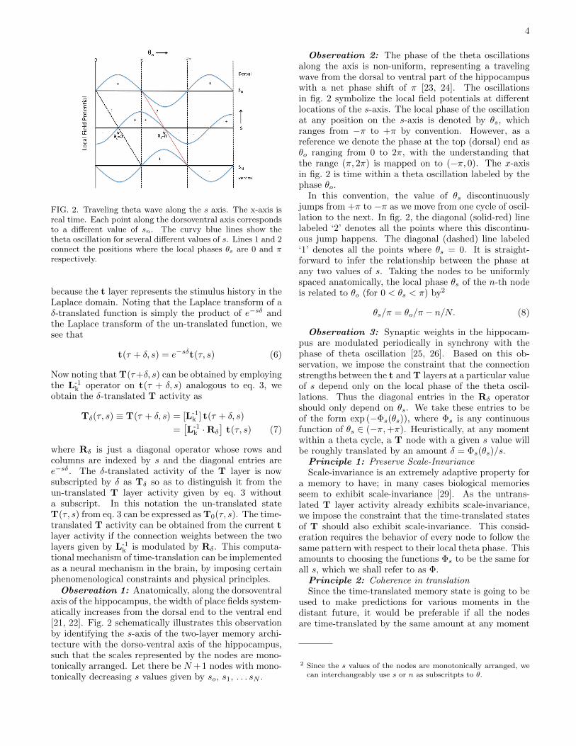
FIG. 2. Traveling theta wave along the s axis. The x-axis isreal time. Each point along the dorsoventral axis correspondsto a different value of sn. The curvy blue lines show thetheta oscillation for several different values of s. Lines 1 and 2connect the positions where the local phases θs are 0 and πrespectively.

because the t layer represents the stimulus history in theLaplace domain. Noting that the Laplace transform of aδ-translated function is simply the product of e−sδ andthe Laplace transform of the un-translated function, wesee that

t(τ + δ, s) = e−sδt(τ, s) (6)

Now noting that T(τ+δ, s) can be obtained by employingthe L-1

k operator on t(τ + δ, s) analogous to eq. 3, weobtain the δ-translated T activity as

Tδ(τ, s) ≡ T(τ + δ, s) = [L-1k ] t(τ + δ, s)

=[L-1

k ·Rδ

]t(τ, s) (7)

where Rδ is just a diagonal operator whose rows andcolumns are indexed by s and the diagonal entries aree−sδ. The δ-translated activity of the T layer is nowsubscripted by δ as Tδ so as to distinguish it from theun-translated T layer activity given by eq. 3 withouta subscript. In this notation the un-translated stateT(τ, s) from eq. 3 can be expressed as T0(τ, s). The time-translated T activity can be obtained from the current tlayer activity if the connection weights between the twolayers given by L-1

k is modulated by Rδ. This computa-tional mechanism of time-translation can be implementedas a neural mechanism in the brain, by imposing certainphenomenological constraints and physical principles.

Observation 1: Anatomically, along the dorsoventralaxis of the hippocampus, the width of place fields system-atically increases from the dorsal end to the ventral end[21, 22]. Fig. 2 schematically illustrates this observationby identifying the s-axis of the two-layer memory archi-tecture with the dorso-ventral axis of the hippocampus,such that the scales represented by the nodes are mono-tonically arranged. Let there be N +1 nodes with mono-tonically decreasing s values given by so, s1, . . . sN .

Observation 2: The phase of the theta oscillationsalong the axis is non-uniform, representing a travelingwave from the dorsal to ventral part of the hippocampuswith a net phase shift of π [23, 24]. The oscillationsin fig. 2 symbolize the local field potentials at differentlocations of the s-axis. The local phase of the oscillationat any position on the s-axis is denoted by θs, whichranges from −π to +π by convention. However, as areference we denote the phase at the top (dorsal) end asθo ranging from 0 to 2π, with the understanding thatthe range (π, 2π) is mapped on to (−π, 0). The x-axisin fig. 2 is time within a theta oscillation labeled by thephase θo.

In this convention, the value of θs discontinuouslyjumps from +π to −π as we move from one cycle of oscil-lation to the next. In fig. 2, the diagonal (solid-red) linelabeled ‘2’ denotes all the points where this discontinu-ous jump happens. The diagonal (dashed) line labeled‘1’ denotes all the points where θs = 0. It is straight-forward to infer the relationship between the phase atany two values of s. Taking the nodes to be uniformlyspaced anatomically, the local phase θs of the n-th nodeis related to θo (for 0 < θs < π) by2

θs/π = θo/π − n/N. (8)

Observation 3: Synaptic weights in the hippocam-pus are modulated periodically in synchrony with thephase of theta oscillation [25, 26]. Based on this ob-servation, we impose the constraint that the connectionstrengths between the t and T layers at a particular valueof s depend only on the local phase of the theta oscil-lations. Thus the diagonal entries in the Rδ operatorshould only depend on θs. We take these entries to beof the form exp (−Φs(θs)), where Φs is any continuousfunction of θs ∈ (−π,+π). Heuristically, at any momentwithin a theta cycle, a T node with a given s value willbe roughly translated by an amount δ = Φs(θs)/s.Principle 1: Preserve Scale-InvarianceScale-invariance is an extremely adaptive property for

a memory to have; in many cases biological memoriesseem to exhibit scale-invariance [29]. As the untrans-lated T layer activity already exhibits scale-invariance,we impose the constraint that the time-translated statesof T should also exhibit scale-invariance. This consid-eration requires the behavior of every node to follow thesame pattern with respect to their local theta phase. Thisamounts to choosing the functions Φs to be the same forall s, which we shall refer to as Φ.

Principle 2: Coherence in translationSince the time-translated memory state is going to be

used to make predictions for various moments in thedistant future, it would be preferable if all the nodesare time-translated by the same amount at any moment

2 Since the s values of the nodes are monotonically arranged, wecan interchangeably use s or n as subscritpts to θ.

5

within a theta cycle. If not, different nodes would con-tribute to predictions for different future moments lead-ing to noise in the prediction. However, such a require-ment of global coherence cannot be imposed consistentlyalong with the principle 1 of preserving scale-invariance.3

But in the light of prior work [30, 31] which suggest thatretrieval of memory or prediction happens only in onehalf of the theta cycle,4 we impose the requirement ofcoherence only to those nodes that are all in the positivehalf of the cycle at any moment. That is, δ = Φ(θs)/s isa constant along any vertical line in the region boundedbetween the diagonal lines 1 and 2 shown in fig. 2. Hencefor all nodes with 0 < θs < π, we require

∆ (Φ (θs) /s) = ∆ (Φ (θo − πn/N) /sn) = 0. (9)

For coherence as expressed in eq. 9 to hold at all val-ues of θo between 0 and 2π, Φ(θs) must be an exponentialfunction so that θo can be functionally decoupled fromn; consequently sn should also have an exponential de-pendence on n. So the general solution to eq. 9 when0 < θs < π can be written as

Φ(θs) = Φo exp [bθs] (10)

sn = so(1 + c)−n (11)

where c is a positive number. In this paper, we shall takec � 1, so that the analytic approximation for the L-1

koperator given in terms of the k-th derivative along thes axis in eq. 3 is valid.

Thus the requirement of coherence in time-translationimplies that the s values of the nodes—the timescalesrepresented by the nodes—are spaced out exponentially,which can be referred to as a Weber-Fechner scale, a com-monly used terminology in cognitive science. Remark-ably, this result strongly resonates with a requirementof the exact same scaling when the predictive informa-tion contained in the memory system is maximized in re-sponse to long-range correlated signals [27]. This featureallows this memory system to represent scale-invariantlycoarse grained past information from timescales exponen-tially related to the number of nodes.

The maximum value attained by the function Φ(θs)is at θs = π, and the maximum value is Φmax =Φo exp [bπ], such that Φmax/Φo = so/sN and b =(1/π) log (Φmax/Φo). To ensure continuity around θs =0, we take the eq. 10 to hold true even for θs ∈ (−π, 0).

3 This is easily seen by noting that each node will have a maxi-mum translation inversely proportional to its s-value to satisfyprinciple 1.

4 This hypothesis follows from the observation that while bothsynaptic transmission and synaptic plasticity are modulated bytheta phase, they are out of phase with one another. That is,while certain synapses are learning, they are not communicatinginformation and vice versa. This led to the hypothesis that thephases where plasticity is optimal are specialized for encodingwhereas the phases where transmission is optimal are specializedfor retrieval.

However, since notationally θs makes a jump from +π to−π, Φ(θs) would exhibit a discontinuity at the diagonalline 2 in fig. 2 from Φmax (corresponding to θs = π) toΦmin = Φ2

o/Φmax (corresponding to θs = −π).Given these considerations, at any instant within a

theta cycle, referenced by the phase θo, the amount δby which the memory state is time-translated can be de-rived from eq. 8 and 10 as

δ(θo) = (Φo/so) exp [bθo]. (12)

Analogous to having the past represented on a Weber-Fechner scale, the translation distance δ into the futurealso falls on a Weber-Fechner scale as the theta phaseis swept from 0 to 2π. In other words, the amount oftime spent within a theta cycle for larger translations isexponentially smaller.

To emphasize the properties of the time-translated Tstate, consider the stimulus to be a Dirac delta functionat τ = 0. From eq. 7, we can express the T layer activityanalogous to eq. 4.

Tδ(τ, s) 's

k![sτ + Φ (θs)]

ke−[sτ+Φ(θs)] (13)

Notice that eqs. 8 and 12 specify a unique relationshipbetween δ and θs for any given s. The r.h.s. above isexpressed in terms of θs rather than δ so as to shed lighton the phenomenon of phase precession.

Since Tδ(τ, s) depends on both τ and θs only via thesum [sτ + Φ (θs)], a given node will show identical activ-ity for various combinations of τ and θs.

5 For instance,a node would achieve its peak activity when τ is signifi-cantly smaller than its timescale (k/s) only when Φ(θs)is large—meaning θs ' +π. And as τ increases towardsthe timescale of the node, the peak activity graduallyshifts to earlier phases all the way to θs ' −π. An im-portant consequence of imposing principle 1 is that therelationship between θs and τ on any iso-activity contouris scale-invariant. That is, every node behaves similarlywhen τ is rescaled by the timescale of the node. We shallfurther pursue the analogy of this phenomenon of phaseprecession with neurophysiological findings in the nextsection (fig. 4).

C. Timeline of Future Prediction

At any moment, Tδ (eq. 13) can be used to predict thestimuli expected at a future moment. Consequently, as δis swept through within a theta cycle, a timeline of futurepredictions can be simulated in an orderly fashion, suchthat predictions for closer events occur at earlier phases

5 While representing timescales much larger than the period of atheta cycle, τ can essentially be treated as a constant within asingle cycle. In other words, θs and τ in eq. 7 can be treated asindependent, although in reality the phases evolve in real time.

6

(smaller θo) and predictions of distant events occur atlater phases. In order to predict from a time-translatedstate Tδ, we need a prediction mechanism. For our pur-poses, we consider here a very simple form of learning andprediction, Hebbian association. In this view, an event islearned (or an association formed in long term memory)by increasing the connection strengths between the neu-rons representing the currently-experienced stimulus andthe neurons representing the recent past events (T0). Be-cause the T layer activity contains temporal informationabout the preceding stimuli, simple associations betweenT0 and the current stimulus are sufficient to encode andexpress well-timed predictions [19]. In particular, theterm Hebbian implies that the change in each connectionstrength is proportional to the product of pre-synapticactivity—in this case the activity of the correspondingnode in the T layer—and post-synaptic activity corre-sponding to the current stimulus. Given that the associ-ations are learned in this way, we define the prediction ofa particular stimulus to be the scalar product of its asso-ciation strengths with the current state of T. In this way,the scalar product of association strengths and a trans-lated state Tδ can be understood as the future predictionof that stimulus.

Consider the thought experiment where a conditionedstimulus cs is consistently followed by another stimulus,a or b, after a time τo. Later when cs is repeated (at atime τ = 0), the subsequent activity in the T nodes canbe used to generate predictions for the future occurrenceof a or b. The connections to the node correspondingto a will be incremented by the state of T0 when a ispresented; the connections to the node corresponding tob will be incremented by the state of T0 when b is pre-sented. In the context of Hebbian learning, the predictionfor the stimulus at a future time as a function of τ andτo is obtained as the sum of Tδ activity of each nodemultiplied by the learned association strength (T0):

pδ(τ, τo) =

N∑n=`

Tδ (τ, sn) T0 (τo, sn) /swn . (14)

The factor swn (for any w) allows for differential associ-ation strengths for the different s nodes, while still pre-serving the scale invariance property. Since δ and θo aremonotonically related (eq. 12), the prediction pδ for vari-ous future moments happens at various phases of a thetacycle.

Recall that all the nodes in the T layer are coherentlytime-translated only in the positive half of the theta cy-cle. Hence for computing future predictions based ona time-translated state Tδ, only coherent nodes shouldcontribute. In fig. 2, the region to the right of diagonalline 2 does not contribute to the prediction. The lowerlimit ` in the summation over the nodes given in eq. 14is the position of the diagonal line 2 in fig. 2 marking theposition of discontinuity where θs jumps from +π to −π.

In the limit when c → 0, the s values of neighboringnodes are very close and the summation can be approx-

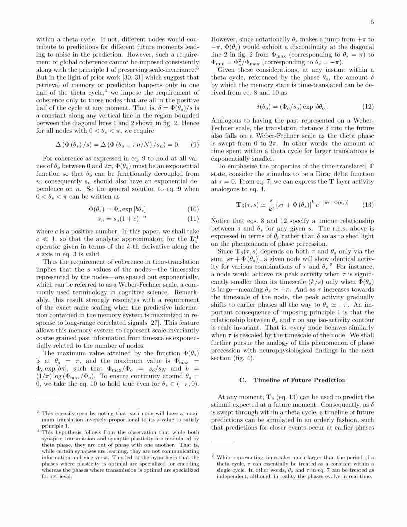
FIG. 3. Future timeline. Eq. 16 is plotted as a function of δ.During training, the cs was presented at τo = 3 before a andτo = 7 before b. Left: Immediately after presentation of thecs, the predictions for a and b are ordered on the δ axis. Notethat the prediction for b approximates a rescaled version ofthat for a. Right: The prediction for b is shown for varyingtimes after presentation of cs. With the passage of time, theprediction of b becomes stronger and more imminent. In thisfigure, Φmax = 10, Φo = 1, k = 10, so = 10, sN = 1, andw = 1.

imated by an integral. Defining x = sτo and y = τ/τoand v = δ/τo, the above summation can be rewritten as

pδ(τ, τo) 'τw−2o

k!2

∫ xu

xmin

x2k+1−w(y + v)ke−x(1+y+v) dx

(15)Here xmin = sNτo, and xu = soτo for 0 < θo < π andxu = Φmaxτo/δ for π < θo < 2π. The integral can beevaluated in terms of lower incomplete gamma functionsto be

pδ(τ, τo) 'τw−2o

k!2[(τ + δ)/τo]

k

[1 + (τ + δ)/τo]C×

(Γ [C, (τo + τ + δ)U ]− Γ [C, (τo + τ + δ)sN ]) ,(16)

where C = 2k + 2− w and Γ[., .] is the lower incompletegamma function. For θo < π (i.e., when δ < Φmax/so),U = so and for θo > π (i.e., when δ > Φmax/so), U =Φmax/δ.

Figure 3 provides a graphical representation of somekey properties of eq. 16. The figure assumes that thecs is followed by a after τo = 3 and followed by b afterτo = 7. The left panel shows the predictions for both aand b as a function of δ immediately after presentationof cs. The prediction for a appears at smaller δ and witha higher peak than the prediction for b. The value of waffects the relative sizes of the peaks. The right panelshows how the prediction for b changes with the passageof time after presentation of the cs. As τ increases fromzero and the cs recedes into the past, the prediction ofb peaks at smaller values of δ, corresponding to moreimminent future times. In particular when τo is muchsmaller than the largest (and larger than the smallest)timescale represented by the nodes, then the shape ofpδ remains the same when δ and τ are rescaled by τo.

7

Under these conditions, the timeline of future predictionsgenerated by pδ is scale-invariant.

Since δ is in one-to-one relationship with θo, as a pre-dicted stimulus becomes more imminent, the activity cor-responding to that predicted stimulus should peak at ear-lier and earlier phases. Hence a timeline of future pre-dictions can be constructed from pδ as the phase θo isswept from 0 to 2π. Moreover the cells representing pδshould show phase precession with respect to θo. Un-like cells representing Tδ, which depend directly on theirlocal theta phase, θs, the phase precession of cells rep-resenting pδ should depend on the reference phase θo atthe dorsal end of the s-axis. We shall further connectthis neurophysiology in the next section (fig. 6).

III. COMPARISONS WITHNEUROPHYSIOLOGY

The mathematical development focused on two entitiesTδ and pδ that change their value based on the thetaphase (eqs. 13 and 16). In order to compare these toneurophysiology, we need to have some hypothesis link-ing them to the activity of neurons from specific brainregions. We emphasize that although the developmentin the preceding section was done with respect to time,all of the results generalize to one-dimensional positionas well (eq. 5, [20]). The overwhelming majority of ev-idence for phase precession comes from studies of placecells (but see [8]). Here we compare the properties ofTδ to phase precession in hippocampal neurons and theproperties of pδ to a study showing phase precession inventral striatum [32].6

Due to various analytic approximations, the activityof nodes in the T layer as well as the activity of thenodes representing future prediction (eqs. 13 and 16) areexpressed as smooth functions of time and theta phase.However, neurophysiologically, discrete spikes (action po-tentials) are observed. In order to facilitate compari-son of the model to neurophysiology, we adopt a simplestochastic spike-generating method. In this simplistic ap-proach, the activity of the nodes given by eqs. 13 and 16are taken to be proportional to the instantaneous proba-bility for generating a spike. The probability of generat-ing a spike at any instant is taken to be the instantaneousactivity divided by the maximum activity achieved bythe node if the activity is greater than 60% of the maxi-mum activity. In addition, we add spontaneous stochas-tic spikes at any moment with a probability of 0.05. Forall of the figures in this section, the parameters of themodel are set as k = 10, Φmax = 10, w = 2, Φo = 1,sN = 1, so = 10.

This relatively coarse level of realism in spike gener-ation from the analytic expressions is probably appro-

6 This is not meant to preclude the possibility that pδ could becomputed at other parts of the brain as well.

a b

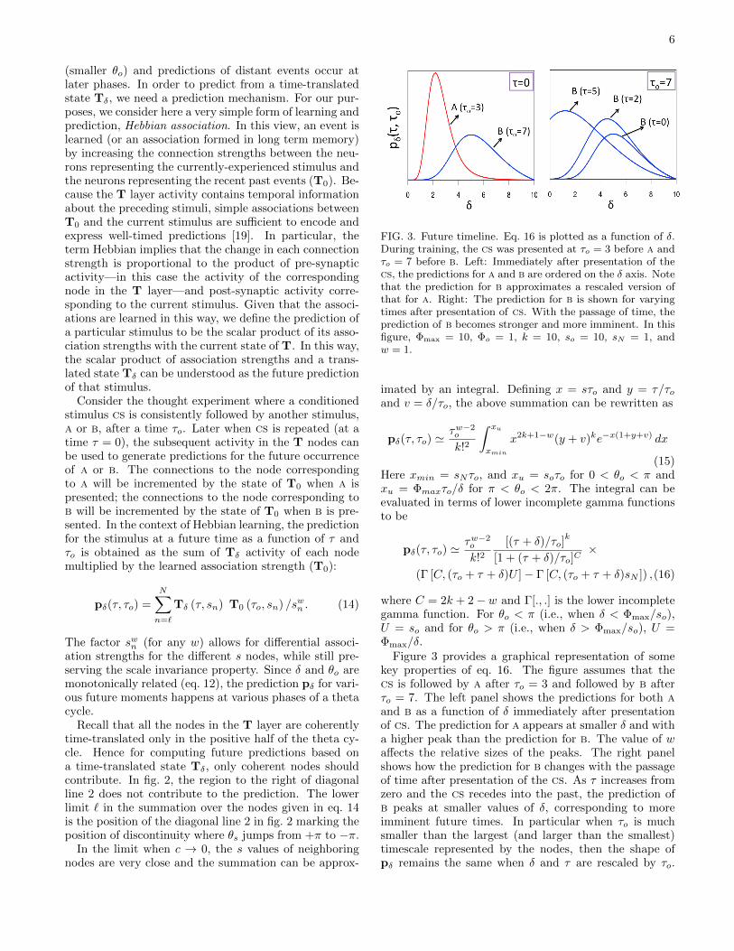
FIG. 4. a. Neurophysiological data showing phase precession.Each spike fired by a place cell is shown as a function of itsposition along a linear track (x-axis) and the phase of localtheta (y-axis). After Mehta, et al., 2002. b. Simulated spikesfrom a node in the T layer described by eq. 13 as a functionof τ and local phase θs. The curvature is a consequence ofeq. 10. See text for details.

priate to the resolution of the experimental data. Thereare some experimental challenges associated with exactlyevaluating the model. First, theta phase has to be es-timated from a noisy signal. Second, phase precessionresults are typically shown as averaged across many tri-als. It is not necessarily the case that the average isrepresentative of an individual trial (although this is thecase at least for phase-precessing cells in medial entorhi-nal cortex [33]). Finally, the overwhelming majority ofphase precession experiments utilize extracellular meth-ods, which cannot perfectly identify spikes from individ-ual neurons.

A. Hippocampal phase precession

It is clear from eq. 13 that the activity of nodes in theT layer depends on both θs and τ . Figure 4 shows phaseprecession data from a representative cell (Fig. 4a, [34])and spikes generated from eq. 13 (Fig. 4b). The modelgenerates a characteristic curvature for phase precession,a consequence of the exponential form of the function Φ(eq. 10). The example cell chosen in fig. 4 shows roughlythe same form of curvature as that generated by themodel. While it should be noted that there is some vari-ability across cells, careful analyses have led computa-tional neuroscientists to conclude that the canonical formof phase precession resembles this representative cell. Forinstance, a detailed study of hundreds of phase-precessingneurons [35] constructed averaged phase-precession plotsusing a variety of methods and found a distinct curva-ture that qualitatively resembles this neuron. Becauseof the analogy between time and one-dimensional posi-tion (eq. 5), the model yields the same pattern of phaseprecession for time cells and place cells.

The T layer activity represented in fig. 4a is scale-invariant; note that the x-axis is expressed in units ofthe scale of the node (k/s). It is known that the spa-tial scale of place fields changes systematically along thedorsoventral axis of the hippocampus. Place cells in thedorsal hippocampus have place fields of the order of a few

8

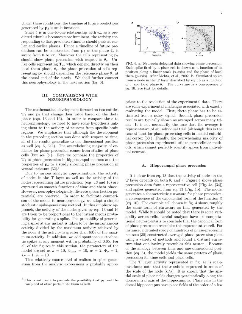
FIG. 5. Place cells along the dorsoventral axis of the hip-pocampus have place fields that increase in size. a. The threepanels show the activity of place cells recorded at the dorsal,intermediate and ventral segments of the hippocampus, whena rat runs along an 18 m track. After Kjelstrup, et al., (2008).Each spike the cell fired is shown as a function of position andthe local theta phase at the cell’s location when it fires (recallthat theta phase is not constant across the dorsoventral axis).Regardless of the width of the place field, neurons at all lo-cations along the dorsoventral axis phase precess through thesame range of local theta phases. b. According to the model,phase precession extends over the same range of values of localtheta θs regardless of the value of s, which sets the scale for aparticular node. As a consequence, cells with different valuesof s show time/place fields of different size but phase precessover the same range of local theta. For the three figures, svalues of the nodes are set to .1, .22, and .7 respectively, andthey are assumed to respond to landmarks at location 4, 11,and 3 meters respectively from one end of the track.

centimeters whereas place cells at the ventral end haveplace fields as large as a few meters (fig. 5a) [21, 22].However, all of them show the same pattern of preces-sion with respect to their local theta phase—the phasemeasured at the same electrode that records a given placecell (fig. 5). Recall that at any given moment, the localphase of theta oscillation depends on the position alongthe dorsoventral axis [23, 24], denoted as the s-axis inthe model.

Figure 5a shows the activity of three different placecells in an experiment where rats ran down a long trackthat extended through open doors connecting three test-ing rooms [22]. The landmarks controlling a particularplace cell’s firing may have been at a variety of locationsalong the track. Accordingly, fig. 5b shows the activity ofcells generated from the model with different values of sand with landmarks at various locations along the track(described in the caption). From fig. 5 it can be qualita-tively noted that phase precession of different cells onlydepends on the local theta phase and is unaffected bythe spatial scale of firing. This observation is perfectlyconsistent with the model.

a b

Start position Reward position

Firin

g ra

te (H

z)

HC

thet

a ph

ase

Ramp cell

Reward position Start position -π

π

0

2π

3π

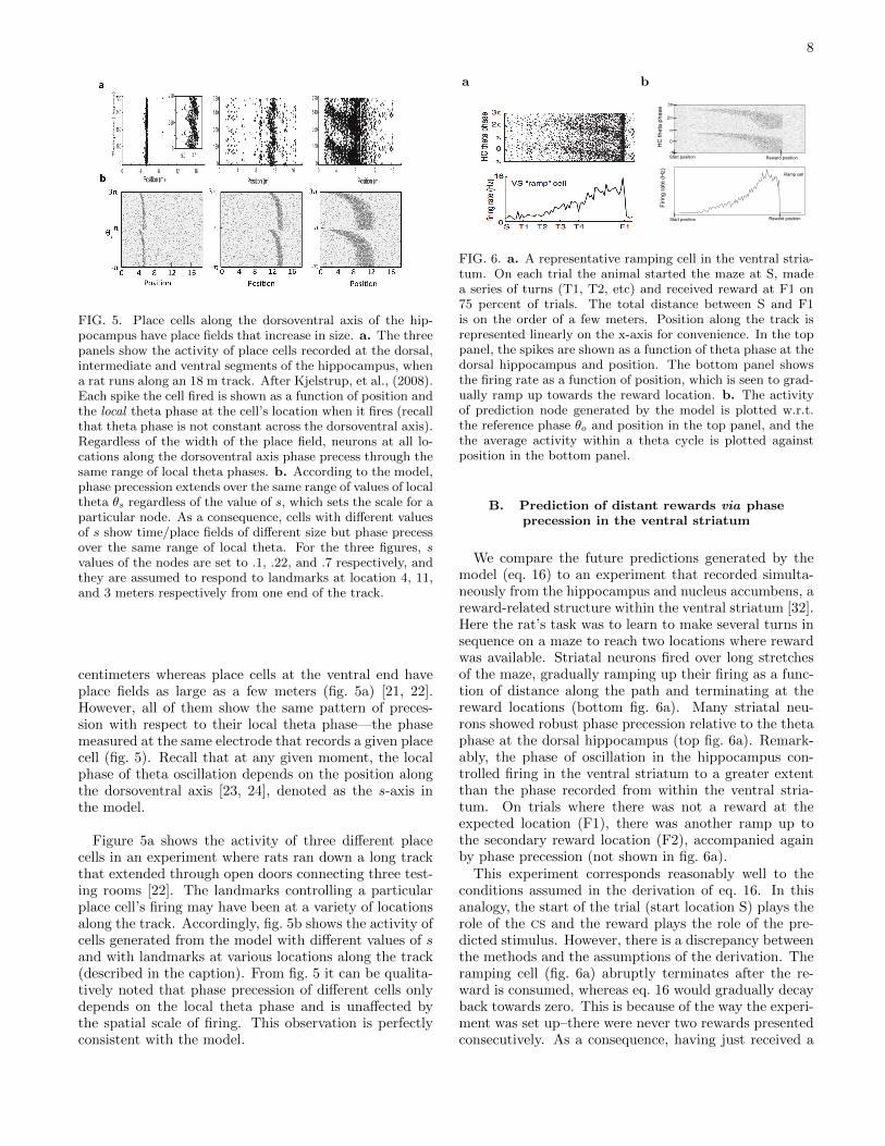
FIG. 6. a. A representative ramping cell in the ventral stria-tum. On each trial the animal started the maze at S, madea series of turns (T1, T2, etc) and received reward at F1 on75 percent of trials. The total distance between S and F1is on the order of a few meters. Position along the track isrepresented linearly on the x-axis for convenience. In the toppanel, the spikes are shown as a function of theta phase at thedorsal hippocampus and position. The bottom panel showsthe firing rate as a function of position, which is seen to grad-ually ramp up towards the reward location. b. The activityof prediction node generated by the model is plotted w.r.t.the reference phase θo and position in the top panel, and thethe average activity within a theta cycle is plotted againstposition in the bottom panel.

B. Prediction of distant rewards via phaseprecession in the ventral striatum

We compare the future predictions generated by themodel (eq. 16) to an experiment that recorded simulta-neously from the hippocampus and nucleus accumbens, areward-related structure within the ventral striatum [32].Here the rat’s task was to learn to make several turns insequence on a maze to reach two locations where rewardwas available. Striatal neurons fired over long stretchesof the maze, gradually ramping up their firing as a func-tion of distance along the path and terminating at thereward locations (bottom fig. 6a). Many striatal neu-rons showed robust phase precession relative to the thetaphase at the dorsal hippocampus (top fig. 6a). Remark-ably, the phase of oscillation in the hippocampus con-trolled firing in the ventral striatum to a greater extentthan the phase recorded from within the ventral stria-tum. On trials where there was not a reward at theexpected location (F1), there was another ramp up tothe secondary reward location (F2), accompanied againby phase precession (not shown in fig. 6a).

This experiment corresponds reasonably well to theconditions assumed in the derivation of eq. 16. In thisanalogy, the start of the trial (start location S) plays therole of the cs and the reward plays the role of the pre-dicted stimulus. However, there is a discrepancy betweenthe methods and the assumptions of the derivation. Theramping cell (fig. 6a) abruptly terminates after the re-ward is consumed, whereas eq. 16 would gradually decayback towards zero. This is because of the way the experi-ment was set up–there were never two rewards presentedconsecutively. As a consequence, having just received a

9

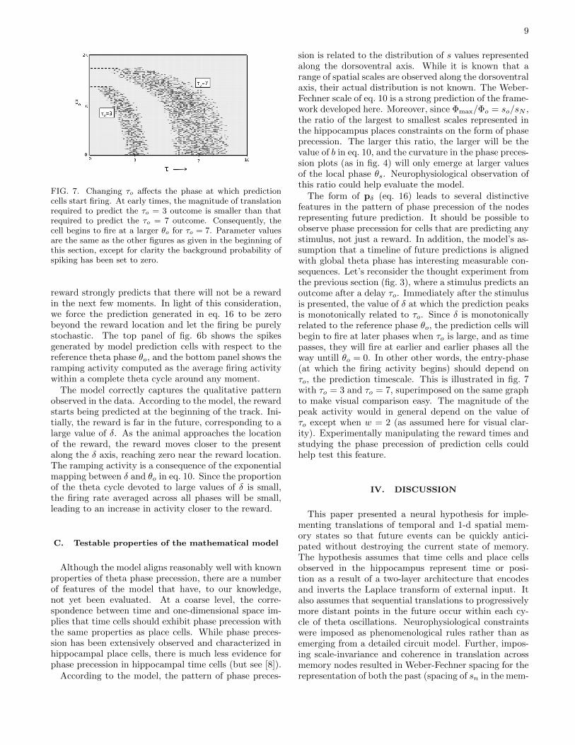
FIG. 7. Changing τo affects the phase at which predictioncells start firing. At early times, the magnitude of translationrequired to predict the τo = 3 outcome is smaller than thatrequired to predict the τo = 7 outcome. Consequently, thecell begins to fire at a larger θo for τo = 7. Parameter valuesare the same as the other figures as given in the beginning ofthis section, except for clarity the background probability ofspiking has been set to zero.

reward strongly predicts that there will not be a rewardin the next few moments. In light of this consideration,we force the prediction generated in eq. 16 to be zerobeyond the reward location and let the firing be purelystochastic. The top panel of fig. 6b shows the spikesgenerated by model prediction cells with respect to thereference theta phase θo, and the bottom panel shows theramping activity computed as the average firing activitywithin a complete theta cycle around any moment.

The model correctly captures the qualitative patternobserved in the data. According to the model, the rewardstarts being predicted at the beginning of the track. Ini-tially, the reward is far in the future, corresponding to alarge value of δ. As the animal approaches the locationof the reward, the reward moves closer to the presentalong the δ axis, reaching zero near the reward location.The ramping activity is a consequence of the exponentialmapping between δ and θo in eq. 10. Since the proportionof the theta cycle devoted to large values of δ is small,the firing rate averaged across all phases will be small,leading to an increase in activity closer to the reward.

C. Testable properties of the mathematical model

Although the model aligns reasonably well with knownproperties of theta phase precession, there are a numberof features of the model that have, to our knowledge,not yet been evaluated. At a coarse level, the corre-spondence between time and one-dimensional space im-plies that time cells should exhibit phase precession withthe same properties as place cells. While phase preces-sion has been extensively observed and characterized inhippocampal place cells, there is much less evidence forphase precession in hippocampal time cells (but see [8]).

According to the model, the pattern of phase preces-

sion is related to the distribution of s values representedalong the dorsoventral axis. While it is known that arange of spatial scales are observed along the dorsoventralaxis, their actual distribution is not known. The Weber-Fechner scale of eq. 10 is a strong prediction of the frame-work developed here. Moreover, since Φmax/Φo = so/sN ,the ratio of the largest to smallest scales represented inthe hippocampus places constraints on the form of phaseprecession. The larger this ratio, the larger will be thevalue of b in eq. 10, and the curvature in the phase preces-sion plots (as in fig. 4) will only emerge at larger valuesof the local phase θs. Neurophysiological observation ofthis ratio could help evaluate the model.

The form of pδ (eq. 16) leads to several distinctivefeatures in the pattern of phase precession of the nodesrepresenting future prediction. It should be possible toobserve phase precession for cells that are predicting anystimulus, not just a reward. In addition, the model’s as-sumption that a timeline of future predictions is alignedwith global theta phase has interesting measurable con-sequences. Let’s reconsider the thought experiment fromthe previous section (fig. 3), where a stimulus predicts anoutcome after a delay τo. Immediately after the stimulusis presented, the value of δ at which the prediction peaksis monotonically related to τo. Since δ is monotonicallyrelated to the reference phase θo, the prediction cells willbegin to fire at later phases when τo is large, and as timepasses, they will fire at earlier and earlier phases all theway untill θo = 0. In other other words, the entry-phase(at which the firing activity begins) should depend onτo, the prediction timescale. This is illustrated in fig. 7with τo = 3 and τo = 7, superimposed on the same graphto make visual comparison easy. The magnitude of thepeak activity would in general depend on the value ofτo except when w = 2 (as assumed here for visual clar-ity). Experimentally manipulating the reward times andstudying the phase precession of prediction cells couldhelp test this feature.

IV. DISCUSSION

This paper presented a neural hypothesis for imple-menting translations of temporal and 1-d spatial mem-ory states so that future events can be quickly antici-pated without destroying the current state of memory.The hypothesis assumes that time cells and place cellsobserved in the hippocampus represent time or posi-tion as a result of a two-layer architecture that encodesand inverts the Laplace transform of external input. Italso assumes that sequential translations to progressivelymore distant points in the future occur within each cy-cle of theta oscillations. Neurophysiological constraintswere imposed as phenomenological rules rather than asemerging from a detailed circuit model. Further, impos-ing scale-invariance and coherence in translation acrossmemory nodes resulted in Weber-Fechner spacing for therepresentation of both the past (spacing of sn in the mem-

10

ory nodes) and the future (the relationship between δ andθo). Apart from providing cognitive flexibility in access-ing a timeline of future predictions at any moment, thecomputational mechanism described qualitative featuresof phase precession in the hippocampus and in the ventralstriatum. Additionally, we have also pointed out certaindistinctive features of the model that can be tested withexisting technology.

A. Approaching a physics of the brain

Given recent and planned advances in the ability tomeasure activity of the brain at an unprecedented levelof detail, the question of whether a satisfactory theo-retical physics of the brain can be developed is increas-ingly pressing [36]. Thus far, the dominant approach is tospecify model neurons of some degree of complexity andsome form of interactions between them and then studythe statistical properties of the network as an emergentproperty. The model neurons can range from extremelysimple bistable units [37–40], or describe the neuronsby a continuous firing-rate model [41–44] or more de-tailed integrate-and-fire neurons [45, 46]. Continuousmodels are usually studied by examining properties ofthe connection matrix which can enable the capacity ofthe memory to be studied analytically and understandother emergent properties. Integrate-and-fire networkscan demonstrate non-trivial changes in their qualitativemacroscopic behavior as a few parameters are changedparametrically. These approaches all share the propertythat they start with a mechanistic description of elementson a small scale and examine the collective behavior on alarger scale. However, the scale at which these networkscan be considered still falls well short of the scale of theentire brain. While recent work has made progress onunderstanding the coupling between scales controlled bya small number of “stiff” parameters [47, 48], it seemslikely that this emergent approach is unlikely to result inan elegant description of the function of the brain, withmultiple interacting heterogeneous regions.

The approach to the physics of the brain taken inthis paper is very different. Rather than specifying mi-croscopic model neurons and then deriving their macro-scopic behavior from first principles, this paper takes amore top-down approach. Known facts of large-scale neu-rophysiology (e.g., theta oscillations are a traveling wave)enter as phenomenological constraints. Considering thecomputational function of the entire system, we applyphenomenological constraints on the output of the com-putation (e.g., scale-invariance, coherence). The resultis a formalism that describes a hypothesis for the large-scale computational function of a large segment of thebrain (the hippocampus and striatum are distant struc-tures). Although the formalism was not derived from firstprinciples, we can still evaluate whether it is consistentwith the physical brain by comparing the equations toneurophysiological findings. And, to the extent the hy-

pothesis is correct, the formalism provides a frameworkfor further theoretical physics of the brain. For instance,generalizing this formalism to 2-dimensions in the caseof spatial navigation (or perhaps N dimensions in a moregeneral computational sense) may result in a set of richand interesting problems.

The challenge in building microscopic models and de-riving their emergent properties is that unless we knowwhat macroscopic computational properties the brain ac-tually exhibits we can never be certain that the micro-scopic properties are correct. In contrast, in the contextof the current approach, the phenomenological equationscan serve as targets for emergent network studies. Forinstance, the derivation here requires a set of integratorswith rate constants s aligned on an anatomical axis withsome tolerance. A solution that derives this phenomeno-logical constraint as an emergent property of a network isguaranteed to align with the larger framework for scale-invariant prediction of the future developed here. In thisway, the macroscopic phenomenological approach takenhere may prove to be a powerful complement to more tra-ditional approaches in formulating a satisfactory physicsof the brain.

B. Computational Advantages

Other proposals for coding temporal memory have re-ceived attention from the physics community [43, 49].However, these approaches do not yield sequentially-activated time cells, nor place coding. The property ofthe T layer that different nodes represent the stimulusvalue from various delays (past moments) is reminiscentof a shift register (or delay-line or synfire chain). How-ever, the two layer network encoding and inverting theLaplace transform of stimulus has several significant com-putational advantages over a shift register representation.

(i) In the current two-layer network, the spacing of svalues of the nodes can be chosen freely. By choosing ex-ponentially spaced s-values (Weber-Fechner scaling) asin eq. 10, the T layer can represent memory from ex-ponentially long timescales compared to a shift registerwith equal number of nodes, thus making it extremelyresource-conserving. Although information from longertimescales is more coarse-grained, it turns out that thiscoarse-graining is optimal to represent and predict long-range correlated signals [27].

(ii) The memory representation of this two layer net-work is naturally scale-invariant (eq. 4). To constructa scale-invariant representation from a shift register, theshift register would have to be convolved with a scale-invariant coarse-graining function at each moment, whichwould be computationally very expensive. Moreover, itturns out that any network that can represent such scale-invariant memory can be identified with linear combina-tions of multiple such two layer networks [50].

(iii) Because translation can be trivially performedwhen we have access to the Laplace domain, the two layer

11

network enables translations by an amount δ without se-quentially visiting the intermediate states < δ. This canbe done by directly changing the connection strengthslocally between the two layers as prescribed by diagonalRδ operator for any chosen δ.7 Consequently the physicaltime taken for the translation can be decoupled from themagnitude of translation. One could imagine a shift reg-ister performing a translation operation by an amount δeither by shifting the values sequentially from one node tothe next for δ time steps or by establishing non-local con-nections between far away nodes. The latter would makethe computation very cumbersome because it would re-quire every node in the register to be connected to everyother node (since this should work for any δ), which isin stark contrast with the local connectivity required byour two layer network to perform any translation.

Many previous neurobiological models of phase preces-sion have been proposed [31, 34, 51, 52], and many as-sume that sequentially activated place cells firing within atheta cycle result from direct connections between thosecells [53], not unlike a synfire chain. Although takingadvantage of the Laplace domain in the two layer net-work to perform translations is not the only possibility,it seems to be computationally powerful compared to theobvious alternatives.

C. Translations without theta oscillations

Although this paper focused on sequential translationwithin a theta cycle, translation may also be accom-plished via other neurophysiological mechanisms. Sharpwave ripple (SRW) events last for about 100 ms and areoften accompanied by replay events–sequential firing ofplace cells corresponding to locations different from theanimal’s current location [54–58]. Notably, experimen-talists have also observed preplay events during SWRs,sequential activation of place cells that correspond to tra-jectories that have never been previously traversed, asthough the animal is planning a future path [55, 59]. Be-cause untraversed trajectories could not have been usedto learn and build sequential associations between theplace cells along the trajectory, the preplay activity couldpotentially be a result of a translation operation on theoverall spatial memory representation.

Sometimes during navigation, a place cell correspond-ing to a distant goal location gets activated [57], asthough a finite distance translation of the memory statehad occurred. More interestingly, sometimes a reverse-replay is observed in which place cells are activated inreverse order spreading back from the present location[56]. This is suggestive of translation into the past (asif δ were negative), to implement a memory search. In

7 In this paper we considered sequential translations of various val-ues of δ, since the aim was to construct an entire future timelinerather than to discontinuously jump to a distant future state.

parallel, there is behavioral evidence from humans thatunder some circumstances memory retrieval consists ofa backward scan through a temporal memory represen-tation [60–62] (although this is not neurally linked withSWRs). Mathematically, as long as the appropriate con-nection strength changes prescribed by the Rδ operatorcan be specified, there is no reason translations with neg-ative δ or discontinuous shift in δ could not be accom-plished in this framework. Whether these computationalmechanisms are reasonable in light of the neurophysiol-ogy of sharp wave ripples is an open question.

D. Multi-dimensional translation

This paper focused on translations along one dimen-sion. However it would be useful to extend the formal-ism to multi-dimensional translations. When a rat ma-neuvers through an open field rather than a linear track,phase precessing 2-d place cells are observed [63]. Con-sider the case of an animal approaching a junction alonga maze where it has to either turn left or right. Phaseprecessing cells in the hippocampus indeed predict thedirection the animal will choose in the future [64]. Inorder to generalize the formalism to 2-d translation, thenodes in the network model must not be indexed onlyby s, which codes their distance from a landmark, butalso by the 2-d orientation along which distance is calcu-lated. The translation operation must then specify notjust the distance, but also the instantaneous direction asa function of the theta phase. Moreover, if translationscould be performed on multiple non-overlapping trajecto-ries simultaneously, multiple paths could be searched inparallel, which would be very useful for efficient decisionmaking.

E. Neural representation of predictions

The computational function of pδ (eq. 16) is to rep-resent an ordered set of events predicted to occur in thefuture. Although we focused on ventral striatum herebecause of the availability of phase precession data fromthat structure, it is probable that many brain regions rep-resent future events as part of a circuit involving frontalcortex and basal ganglia, as well as the hippocampus andstriatum [65–71]. There is evidence that theta-like oscil-lations coordinates the activity in many of these brain re-gions [72–75]. For instance, 4 Hz oscillations show phasecoherence between the hippocampus, prefrontal cortexand ventral tegmental area (VTA), a region that signalsthe presence of unexpected rewards [75]. A great deal ofexperimental work has focused on the brain’s response tofuture rewards, and indeed the phase-precessing cells infig. 6 appear to be predicting the location of the futurereward. The model suggests that pδ should predict anyfuture event, not just a reward. Indeed, neurons that ap-pear to code for predicted stimuli have been observed in

12

the primate inferotemporal cortex [76] and prefrontal cor-tex [77]. Moreover, theta phase coherence between pre-frontal cortex and hippocampus are essential for learningthe temporal relationships between stimuli [78].

ACKNOWLEDGMENTS

The authors gratefully acknowledge helpful discussionswith Michael Hasselmo, Sam McKenzie, Ehren Newman,Jon Ruekmann, Shantanu Jadhav, and Dan Bullock.Supported by NSF PHY 1444389 and the Initiative forthe Physics and Mathematics of Neural Systems.

[1] S. E. Palmer, O. Marre, M. J. Berry, 2nd, and W. Bialek,Proceedings of the National Academy of Sciences USA112, 6908 (2015).

[2] S. Still, D. A. Sivak, A. J. Bell, and G. E. Crooks, Phys-ical Review Letters 109, 120604 (2012).

[3] F. Creutzig, A. Globerson, and N. Tishby, Physical Re-view E 79, 041925 (2009).

[4] K. Friston, Nature Reviews Neuroscience 11, 127 (2010).[5] W. Bialek, Biophysics: searching for principles (Prince-

ton University Press, 2012).[6] E. Save, A. Cressant, C. Thinus-Blanc, and B. Poucet,

Journal of Neuroscience 18, 1818 (1998).[7] R. U. Muller and J. L. Kubie, Journal of Neuroscience 7,

1951 (1987).[8] E. Pastalkova, V. Itskov, A. Amarasingham, and

G. Buzsaki, Science 321, 1322 (2008).[9] C. J. MacDonald, K. Q. Lepage, U. T. Eden, and

H. Eichenbaum, Neuron 71, 737 (2011).[10] P. R. Gill, S. J. Y. Mizumori, and D. M. Smith, Hip-

pocampus 21, 1240 (2011).[11] B. J. Kraus, R. J. Robinson, 2nd, J. A. White, H. Eichen-

baum, and M. E. Hasselmo, Neuron 78, 1090 (2013).[12] H. Eichenbaum, Nature Reviews Neuroscience 15, 732

(2014).[13] H. Eichenbaum and N. J. Cohen, Neuron 83, 764 (2014).[14] H. Eichenbaum, Nature Reviews, Neuroscience 1, 41

(2000).[15] M. E. Hasselmo, L. M. Giocomo, and E. A. Zilli, Hip-

pocampus 17, 1252 (2007).[16] D. L. Schacter, D. R. Addis, and R. L. Buckner, Nature

Reviews, Neuroscience 8, 657 (2007).[17] C. H. Vanderwolf, Electroencephalography and Clinical

Neurophysiology 26, 407 (1969).[18] J. O’Keefe and M. L. Recce, Hippocampus 3, 317 (1993).[19] K. H. Shankar and M. W. Howard, Neural Computation

24, 134 (2012).[20] M. W. Howard, C. J. MacDonald, Z. Tiganj, K. H.

Shankar, Q. Du, M. E. Hasselmo, and H. Eichenbaum,Journal of Neuroscience 34, 4692 (2014).

[21] M. W. Jung, S. I. Wiener, and B. L. McNaughton, Jour-nal of Neuroscience 14, 7347 (1994).

[22] K. B. Kjelstrup, T. Solstad, V. H. Brun, T. Hafting,S. Leutgeb, M. P. Witter, E. I. Moser, and M. B. Moser,Science 321, 140 (2008).

[23] E. V. Lubenov and A. G. Siapas, Nature 459, 534 (2009).[24] J. Patel, S. Fujisawa, A. Berenyi, S. Royer, and

G. Buzsaki, Neuron 75, 410 (2012).[25] B. P. Wyble, C. Linster, and M. E. Hasselmo, Journal

of Neurophysiology 83, 2138 (2000).[26] K. P. Schall, J. Kerber, and C. T. Dickson, Journal of

Neurophysiology 99, 888 (2008).

[27] K. H. Shankar and M. W. Howard, Journal of MachineLearning Research 14, 3753 (2013).

[28] E. Post, Transactions of the American Mathematical So-ciety 32, 723 (1930).

[29] P. D. Balsam and C. R. Gallistel, Trends in Neuroscience32, 73 (2009).

[30] M. E. Hasselmo, C. Bodelon, and B. P. Wyble, NeuralComputation 14, 793 (2002).

[31] M. E. Hasselmo, How We Remember: Brain Mechanismsof Episodic Memory (MIT Press, Cambridge, MA, 2012).

[32] M. A. A. van der Meer and A. D. Redish, Journal ofNeuroscience 31, 2843 (2011).

[33] E. T. Reifenstein, R. Kempter, S. Schreiber, M. B.Stemmler, and A. V. M. Herz, Proceedings of the Na-tional Academy of Sciences 109, 6301 (2012).

[34] M. R. Mehta, A. K. Lee, and M. A. Wilson, Nature 417,741 (2002).

[35] Y. Yamaguchi, Y. Aota, B. L. McNaughton, and P. Lipa,Journal of Neurophysiology 87, 2629 (2002).

[36] J. Beggs, Physical Review Letters 114, 220001 (2015).[37] J. J. Hopfield, Proceedings of the National Academy of

Science, USA 84, 8429 (1982).[38] D. J. Amit, H. Gutfreund, and H. Sompolinsky, Physical

Review Letters 55, 1530 (1985).[39] D. J. Amit, H. Gutfreund, and H. Sompolinsky, Physical

Review A 32, 1007 (1985).[40] D. J. Amit, H. Gutfreund, and H. Sompolinsky, Annals

of Physics 173, 30 (1987).[41] K. Rajan and L. F. Abbott, Physical Review Letters 97,

188104 (2006).[42] S. Ganguli, D. Huh, and H. Sompolinsky, Proceedings of

the National Academy of Sciences of the United Statesof America 105, 18970 (2008).

[43] O. L. White, D. D. Lee, and H. Sompolinsky, PhysicalReview Letters 92, 148102 (2004).

[44] M. Stern, H. Sompolinsky, and L. F. Abbott, PhysicalReview E 90, 062710 (2014).

[45] A. Roxin, N. Brunel, and D. Hansel, Physical ReviewLetters 94, 238103 (2005).

[46] R. Zillmer, N. Brunel, and D. Hansel, Physical ReviewE 79, 031909 (2009).

[47] K. S. Brown and J. P. Sethna, Physical Review E 68,021904 (2003).

[48] B. B. Machta, R. Chachra, M. K. Transtrum, and J. P.Sethna, Science 342, 604 (2013).

[49] H. Z. Shouval, A. Agarwal, and J. P. Gavornik, PhysicalReview Letters 110, 168102 (2013).

[50] K. H. Shankar, Lecture Notes in Artificial intelligence8955, 175 (2015).

[51] J. E. Lisman and O. Jensen, Neuron 77, 1002 (2013).[52] N. Burgess, C. Barry, and J. O’Keefe, Hippocampus 17,

801 (2007).

13

[53] O. Jensen and J. E. Lisman, Learning and Memory 3,279 (1996).

[54] T. J. Davidson, F. Kloosterman, and M. A. Wilson,Neuron 63, 497 (2009).

[55] G. Dragoi and S. Tonegawa, Nature 469, 397 (2011).[56] D. J. Foster and M. A. Wilson, Nature 440, 680 (2006).[57] B. E. Pfeiffer and D. J. Foster, Nature 497, 74 (2013).[58] S. P. Jadhav, C. Kemere, P. W. German, and L. M.

Frank, Science 336, 1454 (2012).

[59] H. F. Olafsdottir, C. Barry, A. B. Saleem, D. Hassabis,and H. J. Spiers, eLife 4, e06063 (2015).

[60] M. J. Hacker, Journal of Experimental Psychology: Hu-man Learning and Memory 15, 846 (1980).

[61] W. E. Hockley, Journal of Experimental Psychology:Learning, Memory, and Cognition 10, 598 (1984).

[62] I. Singh, A. Oliva, and M. W. Howard, PsychologicalScience (revised).

[63] W. E. Skaggs, B. L. McNaughton, M. A. Wilson, andC. A. Barnes, Hippocampus 6, 149 (1996).

[64] A. Johnson and A. D. Redish, Journal of Neuroscience27, 12176 (2007).

[65] W. Schultz, P. Dayan, and P. R. Montague, Science 275,1593 (1997).

[66] J. Ferbinteanu and M. L. Shapiro, Neuron 40, 1227(2003).

[67] S. C. Tanaka, K. Doya, G. Okada, K. Ueda, Y. Okamoto,and S. Yamawaki, Nature Neuroscience 7, 887 (2004).

[68] C. E. Feierstein, M. C. Quirk, N. Uchida, D. L. Sosulski,and Z. F. Mainen, Neuron 51, 495 (2006).

[69] Z. F. Mainen and A. Kepecs, Curr Opin Neurobiol 19,84 (2009).

[70] Y. K. Takahashi, M. R. Roesch, R. C. Wilson, K. Tore-son, P. O’Donnell, Y. Niv, and G. Schoenbaum, NatureNeuroscience 14, 1590 (2011).

[71] J. J. Young and M. L. Shapiro, Journal of Neuroscience31, 5989 (2011).

[72] M. W. Jones and M. A. Wilson, PLoS Biol 3, e402 (2005).[73] C. S. Lansink, P. M. Goltstein, J. V. Lankelma, B. L.

McNaughton, and C. M. A. Pennartz, PLoS Biology 7,e1000173 (2009).

[74] M. van Wingerden, M. Vinck, J. Lankelma, and C. M.Pennartz, Journal of Neuroscience 30, 7078 (2010).

[75] S. Fujisawa and G. Buzsaki, Neuron 72, 153 (2011).[76] K. Sakai and Y. Miyashita, Nature 354, 152 (1991).[77] G. Rainer, S. C. Rao, and E. K. Miller, Journal of Neu-

roscience 19, 5493 (1999).[78] S. L. Brincat and E. K. Miller, Nature Neuroscience 18,

576 (2015).