network topology independent multi-agent dynamic optimal

General rights Copyright and moral rights for the publications made accessible in the public portal are retained by the authors and/or other copyright owners and it is a condition of accessing publications that users recognise and abide by the legal requirements associated with these rights.

Users may download and print one copy of any publication from the public portal for the purpose of private study or research.

You may not further distribute the material or use it for any profit-making activity or commercial gain

You may freely distribute the URL identifying the publication in the public portal If you believe that this document breaches copyright please contact us providing details, and we will remove access to the work immediately and investigate your claim.

Downloaded from orbit.dtu.dk on: Feb 10, 2022

Network Topology Independent Multi-Agent Dynamic Optimal Power Flow forMicrogrids with Distributed Energy Storage Systems

Morstyn, Thomas; Hredzak, Branislav; Agelidis, Vassilios G.

Published in:IEEE Transactions on Smart Grid

Link to article, DOI:10.1109/TSG.2016.2631600

Publication date:2018

Document VersionPeer reviewed version

Link back to DTU Orbit

Citation (APA):Morstyn, T., Hredzak, B., & Agelidis, V. G. (2018). Network Topology Independent Multi-Agent Dynamic OptimalPower Flow for Microgrids with Distributed Energy Storage Systems. IEEE Transactions on Smart Grid, 9(4),3419-3429. https://doi.org/10.1109/TSG.2016.2631600

https://doi.org/10.1109/TSG.2016.2631600

https://orbit.dtu.dk/en/publications/46bce8a2-66b0-475e-a6de-343099878994

https://doi.org/10.1109/TSG.2016.2631600

1949-3053 (c) 2016 IEEE. Personal use is permitted, but republication/redistribution requires IEEE permission. See http://www.ieee.org/publications_standards/publications/rights/index.html for more information.

This article has been accepted for publication in a future issue of this journal, but has not been fully edited. Content may change prior to final publication. Citation information: DOI 10.1109/TSG.2016.2631600, IEEETransactions on Smart Grid

1

Network Topology Independent Multi-Agent

Dynamic Optimal Power Flow for Microgrids with

Distributed Energy Storage SystemsThomas Morstyn, Student Member, IEEE, Branislav Hredzak, Senior Member, IEEE, and

Vassilios G. Agelidis, Fellow, IEEE

Abstract—This paper proposes a multi-agent dynamic optimal

power flow strategy for microgrids with distributed energy

storage systems. The proposed control strategy uses a convex

formulation of the AC dynamic optimal power flow problem

developed from a d-q reference frame voltage-current model and

linear power flow approximations. The convex dynamic optimal

power flow problem is divided between autonomous agents and

solved based on local information and neighbour-to-neighbour

communication over a sparse communication network, using a

distributed primal subgradient algorithm. Each agent is only

required to solve convex quadratic sub-problems, for which

robust and efficient solvers exist, making the control strategy

suitable for receding horizon model predictive control. Also, the

agent sub-problems require limited power network information

and include only a subset of the centralised optimisation problem

decision variables and constraints, providing scalability and data

privacy. Unlike existing distributed optimal power flow methods,

such as alternating direction method of multipliers, under the

proposed control strategy the information required by each agent

is independent of the communication network topology, providing

increased flexibility and robustness. The performance of the

proposed control strategy was verified for an AC microgrid with

distributed lead-acid batteries and intermittent photovoltaic gen-

eration, using an RTDS Technologies real-time digital simulator.

Index Terms—Distributed optimisation, energy management

system, energy storage systems, microgrid, model predictive con-

trol, multi-agent systems, dynamic optimal power flow, quadratic

programming, renewable generation, tertiary control.

I. INTRODUCTION

TECHNOLOGICAL developments and increased scales

of production have dramatically reduced the costs of

distributed renewable generation sources and energy storage

(ES) systems. If properly managed, these sources have the

potential to increase network efficiency, energy reliability and

security, and to reduce pollution [1].

The microgrid concept provides a framework for managing

the integration of these distributed sources [2]. A microgrid is

a collocated set of generation sources, loads and ES systems

that are coordinated to achieve autonomous operation. Since

the microgrid can operate autonomously, it can be controlled

T. Morstyn and B. Hredzak are with the the School of Electrical Engineeringand Telecommunications at The University of New South Wales (UNSW Aus-tralia), Sydney, NSW 2052 Australia (email: [email protected],[email protected]).

V. G. Agelidis is with the Department of Electrical Engineering at theTechnical University of Denmark (DTU), 4000 Roskilde, Denmark (email:[email protected]).

as a dispatchable source when connected to the main grid, and

can continue to operate if islanded.

The standard hierarchical model for microgrid control in-

cludes a centralised energy management system, which solves

the microgrid optimal power flow (OPF) problem and sends

set-points to lower level decentralised controllers at each

source [3]. The OPF problem considers how the distributed

sources should be dispatched to achieve economic objectives,

such as power loss minimisation, while satisfying constraints

imposed by network power quality requirements and device

operating limits [4].

The OPF problem is non-convex, making it computationally

challenging. The computational complexity of the OPF prob-

lem is significantly increased when ES systems are considered,

since their state of charge (SoC) must be optimised over a

prediction horizon [5]. This is described as the dynamic OPF

(DOPF) problem. If predictions of the renewable generation

and load profiles are available, the DOPF problem can be used

for real-time control with a receding horizon model predictive

control (MPC) implementation [3].

The non-convex microgrid DOPF problem can be solved

using dynamic programming [5], [6] or nonlinear program-

ming [7]. However, the computational complexity of these

strategies limits the number of ES systems and the solu-

tion time may be too long to respond to varying renewable

generation sources. The DOPF problem can be simplified

by considering a single ES system [8]–[12] or an ideal real

power transfer model between ES systems [13], [14]. This

provides a convex programming problem, for which fast robust

solvers exist, but neglects the network topology. A DC power

flow approximation can be used to provide a convex DOPF

problem, assuming the network has high X/R ratios [15]. In

this case, the optimisation does not consider reactive power

flows, line losses and bus voltage limits.

The communications and processing infrastructure required

for a centralised control strategy may be impractical for future

microgrids made up of many small distributed renewable

sources and ES systems [16]. Also, data centralisation intro-

duces security and privacy concerns [17].

This motivates the use of multi-agent control. Under a

multi-agent control strategy, autonomous agents use local

information and neighbour-to-neighbour communication over

a sparse communication network to achieve cooperative ob-

jectives [18]. Multi-agent control strategies can provide in-

creased scalability, security and robustness over centralised



2

control strategies [19]. Multi-agent control has been used in

microgrids for secondary control [20]–[22] and SoC balancing

between distributed ES systems [23]–[27].

The main advantages of a multi-agent DOPF strategy, over

a centralised one, can be summarised as: (i) a single point of

failure is removed, (ii) processing and data storage require-

ments can be divided between smaller, low cost distributed

processors, (iii) distributed sources can join/leave the network

without having to update a central coordinator, (iv) distributed

sources can cooperate, while preserving data privacy and (v)

the network cost can be reduced due to shorter link distances

needed for only neighbour-to-neighbour communication.

Multi-agent DOPF strategies are presented in [28]–[31].

These are based on different simplifications of the DOPF

problem, and different communication architectures. In [28],

a convex DOPF problem is solved through iterative opti-

misation sub-problems distributed between microgrid agents,

but a central controller is still required. Multi-agent DOPF

strategies have also been presented based on dual decom-

position algorithms [29] and alternating direction method of

multipliers (ADMM) [30]. These strategies provide scalability

since processing is divided between sparsely connected agents.

However, the robustness and flexibility of a fully distributed

multi-agent strategy are not provided, since each agent’s role

and the communication network between them must match the

underlying power network topology. Also, [29] relies on the

X/R ratios of all lines being closely matched, and [30] uses the

DC power flow approximation, which requires high X/R ratios.

These assumptions do not necessarily hold for low voltage

microgrids. For example, the X/R ratios for the benchmark LV

microgrid from [32] vary from 0.0255 to 0.7028. The strategy

presented in [31] is fully distributed, but is based on an ideal

real power transfer model which does not consider the power

network topology.

This paper proposes a multi-agent DOPF strategy for mi-

crogrids with distributed ES systems and renewable generation

sources. Under the proposed control strategy, autonomous

agents use local information and neighbour-to-neighbour com-

munication over a sparse network to reach agreement on

the optimal power flows that minimise power consumption,

considering the capacity of the distributed ES systems and

renewable sources. The proposed control strategy is based on

a convex formulation of the AC microgrid DOPF problem,

obtained from a d-q reference frame voltage-current model

and linear power flow approximations. The convex formulation

does not assume real and reactive power flows are decoupled,

so line losses and voltage constraints can be explicitly con-

sidered. The convex formulation allows the DOPF problem to

be divided between autonomous microgrid agents and solved

using a distributed primal subgradient algorithm. Compared to

the centralised optimisation problem, the agent sub-problems

contain only a subset of the decision variables and constraints,

and require only local ES system SoC estimates, local re-

newable generation predictions and limited power network

information. This provides scalability, and a basis for data

privacy and security between the agents (e.g. households with

local PV and ES systems). Unlike existing distributed OPF

methods, such as ADMM, the power network information

required by each agent is independent of the communication

network between them, and the agents will reach agreement as

long as they are periodically connected. This has advantages in

terms of flexibility and robustness to communication failures.

The proposed control strategy uses a receding horizon MPC

implementation, making it suitable for real-time control of a

microgrid with intermittent renewable generation sources. The

proposed multi-agent DOPF strategy has been integrated with

low level decentralised droop control to share any power im-

balance resulting from small mismatches between the agents’

decision variables. The performance of the proposed control

strategy was verified for a microgrid with intermittent PV

generation and lead-acid battery ES systems, using an RTDS

Technologies real-time digital simulator.

The rest of this paper is organised as follows. Section II

describes the principle of operation of the proposed control

strategy. The convex DOPF formulation is presented in Section

III. The proposed multi-agent based control strategy is devel-

oped in Section IV by dividing the DOPF problem between the

microgrid agents. Real-time simulation results demonstrating

the performance of the proposed control strategy are presented

in Section V. Section VI concludes the paper.

II. PRINCIPLE OF OPERATION

This study considers an islanded microgrid with distributed

PV and battery ES systems, interfaced with the microgrid

through voltage source converters (VSC). To achieve au-

tonomous operation, the microgrid power balance must be

maintained at all times. The distributed microgrid sources

operate under the standard decentralised f −P , V −Q droop

control, which provides load sharing between the sources

without requiring time-critical communication links [33].

ωi = ω0 −mPi(Pvsci − P ∗vsci),

Voi = V ∗oi − nQi(Qvsci −Q∗

vsci). (1)

ω0 is the nominal microgrid frequency, Pvsci and Qvsci are

the real and reactive powers, mPi and nQi are the droop coef-

ficients, P ∗vsci and Q∗

vsci are the VSC real and reactive power

references and V ∗oi is the nominal output voltage magnitude.

The generated frequency reference ωi and voltage reference

Voi are sent to lower level VSC voltage and current controllers.

The proposed multi-agent DOPF strategy is introduced at a

higher level, to optimise the energy flows between the battery

ES systems. The microgrid has autonomous agents, which

collectively have information on the microgrid power network

topology, renewable generation predictions and battery SoC

estimates, but each agent only has access to a subset of this

information.

The multi-agent DOPF strategy is implemented using re-

ceding horizon MPC, making it suitable for real-time control.

A standard selection for the DOPF sampling period in mi-

crogrids with PV generation is 5 minutes [7]. Each sampling

instant, the agents obtain updated local renewable generation

predictions and SoC estimates. Between sampling instants,

the agents cooperatively solve the DOPF problem based on

the distributed primal subgradient algorithm from [34]. At

each communication sub-interval, the agents solve reduced



3

Cfi

Lfi rfi Lci rci

Llineij

rlineij

PV

Battery

Lloadi

rloadi

(udi,uqi)

(iLdi,iLqi)

(vodi,voqi)

(iodi,ioqi)

(vbdi,vbqi)(iloaddi,iloadqi)

(ilinedij,ilineqij)

(vbdj,vbqj)

Fig. 1. Two bus microgrid segment with a PV and battery ES system, an RLload and an RL line. DC–DC converters interface the PV source and batterywith the DC link of the VSC. The VSC is connected to the microgrid throughan LCL filter.

size optimisation sub-problems (with a reduced number of de-

cision variables and constraints compared with the centralised

problem) using local information and information received

from their neighbours in a sparse communication network.

The agents converge towards the optimal solution as long as

the communication network between them provides periodic

connectivity, giving a measure of robustness to communication

failures.

At the end of each MPC sampling interval, the agents

collocated with distributed PV and battery ES systems use

their local decision variables to generate a real power refer-

ence, reactive power reference and nominal output voltage for

their local VSCs. These are supplied to the lower level droop

control. Then, the MPC prediction horizon recedes by a step,

the agents obtain updated renewable generation predictions

and battery SoC estimates, and begin solving the next sampling

interval’s optimisation.

It is desirable to implement the proposed multi-agent DOPF

strategy with as few communication sub-intervals as possible

to reduce the computation time and amount of exchanged

communication data. However, with a limited number of sub-

intervals, the agents may not converge to an exact solution, and

small mismatches between the agents’ decision variables may

result in a power imbalance. Microgrid disturbances (such as

converter failures) may also result in a power imbalance. In the

case of a power imbalance, the lower level decentralised droop

control will share the microgrid load between the remaining

VSCs.

III. CONVEX DYNAMIC OPTIMAL POWER FLOW

In this section, the DOPF problem is formulated based on a

static synchronous d-q reference frame voltage-current model.

Power flow linearisations are introduced to obtain a convex

optimisation problem.

A. Microgrid Modelling

Consider an islanded microgrid with distributed PV and

battery ES systems, RL loads and RL lines. Let Sbus =1, . . . , Nbus be the set of microgrid buses and Sbatt ⊆ Sbus

be the subset of buses with PV and battery ES systems.

Let Sline be the set of line current flow directions, where

(i, j) ∈ Sline and (j, i) ∈ Sline if there is a line between bus

i and bus j. Let NPi be the power network neighbours of bus

i, where j ∈ NPi if (i, j) ∈ Sline. Fig. 1 shows a two bus

segment of the microgrid. The microgrid state equations are

given by [33],

Lfi

˙[

iLdi

iLqi

]

= −AiLi

[

iLdi

iLqi

]

+

[

udi

uqi

]

−

[

vodivoqi

]

,

Cfi

˙[

vodivoqi

]

= −Avoi

[

vodivoqi

]

+

[

iLdi

iLqi

]

−

[

iodiioqi

]

,

Lci

˙[

iodiioqi

]

= −Aioi

[

iodiioqi

]

+

[

vodivoqi

]

−

[

vbdivbqi

]

, i ∈ Sbatt,

Lloadi

˙[

iloaddiiloadqi

]

= −Ailoadi

[

iloaddiiloadqi

]

+

[

vbdivbqi

]

, i ∈ Sbus,

Llineij

˙[

ilinedijilineqij

]

= −Ailineij

[

ilinedijilineqij

]

+

[

vbdivbqi

]

−

[

vbdjvbqj

]

,

(i, j) ∈ Sline,

AiLi=

[

rfi −ω0Lfi

ω0Lfi rfi

]

, Avoi=

[

0 −ω0Cfi

ω0Cfi 0

]

,

Aioi =

[

rci −ω0Lci

ω0Lci rci

]

, Ailoadi=

[

rloadi −ω0Lloadi

ω0Lloadi rloadi

]

,

Ailineij=

[

rlineij −ω0Llineij

ω0Llineij rlineij

]

. (2)

Respectively, (iLdi, iLqi), (iodi, ioqi), (udi, uqi) and

(vodi, voqi) are the d-q components of the inductor current,

output current, filter input voltage and output voltage of the

PV and battery ES system VSC at bus i. The d-q components

of the voltage and load current for bus i are (vbdi, vbqi) and

(iloaddi, iloadqi). The d-q components for the line current

from bus i to bus j are (ilinedij , ilineqij).

The proposed DOPF strategy controls the microgrid by sup-

plying real power, reactive power and RMS voltage references

to the VSCs each sampling instant, based on SoC estimates

and predictions of the PV generation. Since the DOPF strategy

operates on a much slower time-scale than the microgrid

voltage-current dynamics, a static voltage-current model can

be used to formulate the optimisation problem.

[

iloaddiiloadqi

]

= A−1iloadi

[

vbdivbqi

]

, i ∈ Sbus,

[

ilinedijilineqij

]

= A−1ilineij

([

vbdivbqi

]

−

[

vbdjvbqj

])

, (i, j) ∈ Sline,

[

iodiioqi

]

=

[

iloaddiiloadqi

]

+∑

j∈NPi

[

ilinedijilineqij

]

,

[

vodivoqi

]

=

[

vbdivbqi

]

+Aioi

[

iodiioqi

]

,

[

iLdi

iLqi

]

= Avoi

[

vodivoqi

]

+

[

iodiioqi

]

,

[

udi

uqi

]

=

[

vodivoqi

]

+AiLi

[

iLdi

iLqi

]

, i ∈ Sbatt. (3)

Let vbdq = [vbd1 vbq1 · · · vbdNbusvbqNbus

]T be the vector of

microgrid bus voltages. From the static d-q voltage-current

model (3), the microgrid voltages and currents can be ex-



4

fiL fir

fiCciL cir

Clinki

PV

Pbatti

Ppvi

Battery

dciL

dciL (udi,uqi)

(iLdi,iLqi)

(vodi,voqi)

(iodi,ioqi)

(vbdi,vbqi)

Pvsci, Qvsci

Fig. 2. PV and battery ES system architecture. The PV source and batteryare interfaced through DC–DC converters to the VSC DC link. The VSC isconnected to the microgrid through an LCL filter.

pressed as linear functions of the bus voltages.

[iloaddi iloadqi]T = Giloadi

vbdq, i ∈ Sbus,

[ilinedij ilineqij ]T = Gilineij

vbdq, (i, j) ∈ Sline,

[iLdi iLqi]T = GiLi

vbdq, [udi uqi]T = Gui

vbdq, (4)

[iodi ioqi]T = Gioivbdq, [vodi voqi]

T = Gvoivbdq, i ∈ Sbatt.

Fig. 2 shows a typical architecture for a PV and battery

ES system. The PV source and battery are interfaced through

DC–DC converters to the DC link of a three phase VSC. The

VSC is connected to the microgrid through an LCL filter. The

PV generation source is controlled to operate at its maximum

power point, while the VSC is controlled using decoupled d-q

voltage and current controllers to achieve the frequency and

voltage references set by the droop control. The battery is

operated to maintain the VSC DC link voltage, and therefore

supplies the extra power required to balance the PV generation

with the power exported by the VSC.

The following model is widely used for the battery SoC

dynamics [10], [11], [28]–[31].

SoCi(k + 1) = SoCi(k)−Ts

Ebatti

Pbatti(k),

Pbatti(k) = Pvsci(k)− Ppvi(k), i ∈ Sbatt. (5)

Ebatti is the battery energy capacity, Ts is the sampling period,

Pbatti(k) is the battery output power and Ppvi(k) is the PV

source output power. Note that this model does not include

the limited charging and discharging efficiency of the battery.

The VSC real output power is given by,

Pvsci(k) = iLdi(k)udi(k) + iLqi(k)uqi(k). (6)

The following approximation for the VSC real output power

is used to obtain a linear SoC model, based on a nominal

operating point of (ILdi, ILqi) for the VSC inductor current

and (Udi, Uqi) for the VSC filter input voltage.

Pvsci(k) =[ILdi ILqi]Guivbdq(k) + [Udi Uqi]GiLi

vbdq(k)

− ILdiUdi − ILqiUqi. (7)

Constant power loads can be included in the d-q reference

frame voltage-current model using similar power flow approx-

imations. This is described in the Appendix.

vd / V

LL (Vpu)

0.85 0.9 0.95 1 1.05 1.1 1.15

vq /

VL

L (

Vp

u)

-0.15

-0.1

-0.05

0

0.05

0.1

0.15V

LL min

VLL

max

d-q box const.

Fig. 3. Line to line RMS bus voltage constraints and conservative boxconstraints.

B. Convex Dynamic Optimal Power Flow Formulation

Let τ = 0, . . . , Np − 1 be the optimisation prediction

horizon. The inputs of the optimisation are the battery SoC

estimates SoCi(0), i ∈ Sbatt, and the predicted average PV

generation during each sampling interval of the prediction

horizon, Ppvi(k), i ∈ Sbatt, k ∈ τ .

In this study, the objective selected for the islanded mi-

crogrid is to minimise average power consumption, while

operating the renewable generation sources at their maximum

power point. Minimising power consumption can be desirable

when energy supplies are limited. Conservation voltage re-

duction, i.e. controlling bus voltages towards the lower end

of allowed limits to reduce power consumption, has been

widely applied to achieve this [35]–[39]. Conservation voltage

reduction is naturally provided by the DOPF strategy with a

power consumption minimisation cost function.

The power consumed by the microgrid loads, VSC filters

and lines, over the prediction horizon, are given by,

Jloadi =∑

k∈τ

rloadi(

i2loaddi(k) + i2loadqi(k))

=∑

k∈τ

rloadivTbdq(k)G

Tiloadi

Giloadivbdq(k), (8)

Jvsci =∑

k∈τ

rfi(

i2Ldi(k) + i2Lqi(k))

+ rci(

i2odi(k) + i2oqi(k))

=∑

k∈τ

vTbdq(k)(rfiG

TiLi

GiLi+ rciG

Tioi

Gioi)vbdq(k),

(9)

Jlineij =∑

k∈τ

rlineij(

i2linedij(k) + i2lineqij(k))

=∑

k∈τ

rlineijvTbdq(k)G

Tilineij

Gilineijvbdq(k). (10)

Alternative objectives can be considered depending on the

microgrid. With constant power loads, power loss minimisa-

tion is a more suitable objective. In this case the Jloadi terms

would not be included in the optimisation cost function. In

a microgrid with a mix of conventional generation sources

and battery ES systems, it may be desirable to include battery

depreciation in the cost function. This can be done using an

Ah throughput model for battery lifetime degradation [40].

Let VLL be the nominal microgrid line to line voltage.

Standard microgrid bus voltage limits are 0.9pu to 1.1pu. This



5

requires that,

0.9VLL ≤√

v2bdi(k) + v2bqi(k) ≤ 1.1VLL, i ∈ Sbus, k ∈ τ.

(11)

Assuming nominal d-q bus voltages of (VLL, 0), the quadratic

voltage constraints (11) can be approximated with the follow-

ing box constraints,

0.9VLL ≤vbdi(k) ≤ 1.0954VLL,

−0.1VLL ≤vbqi(k) ≤ 0.1VLL, i ∈ Sbus, k ∈ τ. (12)

Fig. 3 shows the limits on the RMS line to line bus voltages

(11) in the d-q reference frame and the approximate box

constraints (12).

The VSCs should be kept within output power limits to

ensure they are not overloaded. Approximate constraints are

introduced on the VSC real output powers using (7).

Pminvsc ≤ Pvsci(k) ≤ Pmax

vsc , i ∈ Sbatt, k ∈ τ. (13)

Batteries suffer from significant lifetime deterioration when

overcharged or undercharged [41]. Therefore, the batteries

should be operated within SoC limits.

SoCmini...

SoCmini

≤

SoCi(1)...

SoCi(Np)

≤

SoCmaxi...

SoCmaxi

, i ∈ Sbatt.

(14)

The battery SoC values over the prediction horizon can be

expressed as affine functions of the initial SoC, the microgrid

bus voltages and the PV generation, using (5) and (7).

SoCi(1)...

SoCi(Np)

=

SoCi(0)...

SoCi(0)

+

1 0 · · · 0...

. . .. . .

......

. . . 01 · · · · · · 1

gSoCi(0)...

gSoCi(Np − 1)

+

BSoCi 0 · · · 0...

. . .. . .

......

. . . 0BSoCi · · · · · ·BSoCi

vbdq(0)...

vbdq(Np − 1)

,

BSoCi =−Ts

Ebatti

(

[ILdi ILqi]Gui+ [Udi Uqi]GiLi

)

,

gSoCi(k) =Ts

Ebatti

(

ILdiUdi + ILqiUqi + Ppvi(k))

. (15)

The current flowing into each bus must be zero at each time

interval to maintain the microgrid power balance. For buses

with a battery ES system, any mismatch in the line and load

currents will be reflected in the ES system output power. The

following constraints must be introduced for buses without an

ES system.

(

Giloadi+∑

j∈NPi

Gilineij

)

vbdq(k) = 0, i ∈ Sbus, i /∈ Sbatt, k ∈ τ.

(16)

Combining the power consumption functions (8), (9),

(10) and constraints (12), (13), (14), (16), the centralised

microgrid DOPF problem can be formulated as a convex

quadratic program (QP). Let the vector of decision variables

be x ∈ Rm, m = 2NbusNp, the d-q reference frame

bus voltages over the optimisation prediction horizon, i.e.

x = [vTbdq(0) · · · v

Tbdq(Np − 1)]T . The DOPF problem is

given by,

minimisex∈Rm

∑

i∈Sbus

Jloadi +∑

i∈Sbatt

Jvsci +∑

(i,j)∈Sline

1

2Jlineij

subject to (12), (13), (14), (16). (17)

IV. MULTI-AGENT DOPF STRATEGY

Consider autonomous microgrid agents V = 1, . . . , Nagtthat cooperatively solve the DOPF using limited power net-

work information and neighbour-to-neighbour communication.

The agents are connected by a sparse communication net-

work, and share information at sub-intervals between the MPC

sampling instants. The communication network is represented

by a directed graph G(V , E(κ)), with edges E(κ) during sub-

interval κ. An edge (a, b) ∈ E(κ) if there is a communication

link allowing information to flow from agent a to agent b.Let Na(κ) be the neighbours of agent a, where b ∈ Na(κ) if

(b, a) ∈ E(κ). The graph’s weighted adjacency matrix is given

by A(κ) = [wab(κ)] ∈ RNagt×Nagt . The adjacency matrix

diagonals waa(κ) = 1 −∑

b∈Nawab(κ), and for a 6= b, link

weight wab(κ) > 0 if (b, a) ∈ E(κ) and wab(κ) = 0 otherwise.

Under the following communication network conditions, the

DOPF problem (17) can be divided between the autonomous

agents and solved using the distributed primal subgradient

algorithm from [34].

1) Non-Degeneracy: There exists β > 0 such that

waa(κ) = 1 −∑

b∈Nawab(κ) ≥ β, and wab(κ) ∈

0 ∪ [β, 1], a 6= b, for all κ ≥ 0.

2) Balanced Communication:∑Nagt

a=1 wab(κ) = 1 and∑Nagt

b=1 wab(κ) = 1, for all κ ≥ 0.

3) Periodic Strong Connectivity: There is a positive integer

B such that the graph (V ,∪B−1κ=0 E(κ0 + κ)) is strongly

connected for all κ0 ≥ 0.

Each agent has access to a limited amount of power network

information. Let each agent a ∈ V be assigned a subset of

the PV and battery ES systems, S[a]batt ⊆ Sbatt, buses S

[a]bus ⊆

Sbus, and line current flow directions, S[a]line ⊆ Sline. The PV

and battery ES systems are assigned such that, ∪a∈VS[a]batt =

Sbatt. The buses assigned to agent a include those with the

assigned PV and battery ES systems, S[a]bus ⊇ i|i ∈ S

[a]batt. All

buses must be assigned to at least one agent, i.e. ∪a∈VS[a]bus =

Sbus. The agents are assigned the line current flow directions

that have one of their assigned buses as its origin, S[a]line ⊇

(i, j)|i ∈ S[a]bus, (i, j) ∈ Sline.

The information available to each agent depends on the PV

and battery ES systems, buses and line current flow directions

assigned to it. For each PV and battery ES i ∈ S[a]batt, the

agent has access to the VSC filter impedances AiLi, Avoi

, Aioi ,

the current battery SoC estimates SoCi(0) and PV generation

predictions Ppvi(k), k ∈ τ . For each assigned bus i ∈ S[a]bus,

the agent has access to the load impedances Ailoadi. For each

assigned line current flow direction (i, j) ∈ S[a]line, the agent

has access to the line impedances Ailineij.



6

The DOPF cost function is divided between the agents based

on their available power network information.

J [a] =∑

i∈S[a]bus

Jloadi

Nagtbusi

+∑

i∈S[a]batt

Jvsci

Nagtbatti

+∑

(i,j)∈S[a]line

1

2

Jlineij

Nagtlineij

. (18)

Nagtbatti, N

agtbusi, N

agtlineij are the number of agents each PV and

battery ES system, bus and line current flow direction are

respectively assigned to.

Each agent is also assigned a subset of the DOPF con-

straints. The convex constraint set for agent a is given by

X [a] = x ∈ Rm| (19), (20), (21), (22).

0.9VLL ≤ vbdi(k) ≤ 1.0954VLL,

− 0.1VLL ≤ vbqi(k) ≤ 0.1VLL, i ∈ S[a]bus ∪j∈S

[a]bus

NPj , k ∈ τ,

(19)

Pminvsc ≤ Pvsci(k) ≤ Pmax

vsc , i ∈ S[a]batt, k ∈ τ, (20)

Ailoadi

[

vbdi(k)vbqi(k)

]

+∑

j∈NPi

A−1ilineij

([

vbdi(k)vbqi(k)

]

−

[

vbdj(k)vbqj(k)

])

= 0,

i ∈ S[a]bus, i /∈ Sbatt, k ∈ τ, (21)

SoCmini...

SoCmini

≤

SoCi(1)...

SoCi(Np)

≤

SoCmaxi...

SoCmaxi

, i ∈ S[a]batt.

(22)

The sum of the individual agent cost functions are equal to the

centralised DOPF problem cost function, and the intersection

of the agent constraint sets include all of the DOPF problem

constraints. Therefore, the central microgrid DOPF problem

(17) is equivalent to the following separable convex QP,

minimisex∈Rm

∑

a∈V

J [a]

subject to x ∈ ∩a∈VX[a]. (23)

Due to the sparse nature of power networks, only some of

the microgrid bus voltages are relevant to each agent’s cost

function and constraint set. The number of decision variables

for agent a is given by m[a] = 2|S[a]bus ∪i∈S

[a]bus

NPi |Np, the

number of d-q voltages over the prediction horizon for the

buses assigned to the agent and those buses’ neighbours.

A reduced size decision vector for agent a can be obtained

from a linear mapping M[a] : Rm → R

m[a]

, x[a] =M[a](x[a]). A reverse map is also defined for each agent,

M′[a] : Rm[a]

× Rm → R

m, x[a] = M′[a](x[a], v[a]) which

maps the elements of a reduced decision vector x[a] ∈ Rm[a]

back onto a full size decision vector x[a] ∈ Rm, and takes the

remaining elements from v[a] ∈ Rm.

For each agent a ∈ V , an appropriate cost function

J [a] : Rm[a]

→ R is chosen such that J [a](M(x[a])) =J [a](x[a]), ∀x[a] ∈ R

m and constraint set X [a] = x[a] ∈

Rm[a]

| (19), (20), (21), (22).

The distributed primal subgradient algorithm from [34] is

used to solve the multi-agent DOPF problem. The algorithm

has been modified to use the sparse structure of the power

network so that each agent solves reduced size optimisation

sub-problems.

Each agent maintains a local estimate of the full microgrid

decision vector x[a] and initialises it so that x[a](0) ∈ X [a].

At each communication sub-interval, κ ≥ 0, the agents

share their decision vectors with their neighbours and take

a convex combination,

v[a](κ) = waa(κ)x[a](κ) +

∑

b∈Na

wab(κ)x[b](κ). (24)

The convex combination of decision vectors is reduced to the

elements relevant to the agent sub-problem using the linear

map,

v[a](κ) = M[a](

v[a](κ))

. (25)

Each agent then updates their reduced size local decision

vector by making a subgradient step from the convex combi-

nation to reduce their local cost function and projecting the

result onto their local constraint set X [a],

x[a](κ+ 1) = PX[a]

[

v[a](κ)− α(κ)∇J [a](

v[a](κ))]

. (26)

The updated reduced size decision vector and the convex

combination of neighbour decision vectors are used to update

the local full size microgrid decision vector, using the reverse

map,

x[a](κ+ 1) = M′[a](

x[a](κ+ 1), v[a](κ))

. (27)

α(κ) is the distributed primal subgradient algorithm step

size. α(κ) should be chosen so that [34],

limκ→∞

α(κ) = 0,

∞∑

κ=0

α(κ) = ∞,

∞∑

κ=0

α2(κ) < ∞. (28)

Since each agent’s local cost function J [a] and constraint set

X [a] are independent of decision variables in x[a] that are

not in x[a], the proof of convergence from [34] is valid for

the modified algorithm. Therefore, the local agent decision

vectors approach the optimal solution x∗ of the centralised

DOPF problem (17), limκ→∞ ‖x[a](κ)− x∗‖2 = 0,∀a ∈ V .

Each agent solves the projection problem (26) using the

following convex QP,

minimizex[a](κ+1)∈Rm[a]

‖x[a](κ+ 1)− v[a](κ) + α(κ)∇J [a](

v[a](κ))

‖22

subject to x[a](κ+ 1) ∈ X [a]. (29)

The proposed multi-agent DOPF strategy is implemented

using receding horizon MPC. At each optimisation sampling

instant, the microgrid agents obtain estimates of their local

battery SoC and predictions of the average renewable gen-

eration for each interval of the prediction horizon. Under the

distributed primal subgradient algorithm, the agents iteratively

solve their local projection problems and combine their local

decision vector estimates so that they cooperatively converge

towards a solution to the microgrid DOPF problem. After

the number of communication sub-intervals allowed by the

duration of the MPC sampling period, the agents collocated

with PV and battery ES systems generate a local VSC real

power reference, reactive power reference and nominal output



7

TABLE IREAL-TIME SIMULATION PARAMETERS

Np 3 Ts 5min ω0 50Hz

VLL 415V V max 1.1VLL V min 0.9VLL

Ebatt 20kWh SoCmax 100% SoCmin 40%

Pmaxvsc 6kW Pmin

vsc -6kW mP 2.1×10−5

nQ 2.8×10−4 fvsc 2kHz fdcdc 1kHz

rf 0.01Ω Lf 5mH Cf 68µF

rc 0.01Ω Lc 5mH Clink 3.4mF

Ldc 150mH

TABLE IICENTRAL AND MULTI-AGENT DOPF PROBLEM SIZES

Multi-Agent Central

Number of: DOPF Agents DOPF

Buses 1 9

PV+Batt. Systems ≤ 1 5

Line Directions ≤ 3 16

Decision Variables ≤ 24 54

Constraints ≤ 54 192

voltage magnitude for the first interval of the prediction

horizon by solving,

P ∗vsci(0)= u

[a]di (0)i

[a]Ldi(0) + u

[a]qi (0)i

[a]Lqi(0),

Q∗vsci(0)= u

[a]di (0)i

[a]Lqi(0)− u

[a]qi (0)i

[a]Ldi(0),

V ∗oi(0)=

√

v[a]odi(0)

2 + v[a]oqi(0)

2. (30)

The agents send the references to the lower level droop

controllers of their PV and battery ES system VSCs. At

the next optimisation sampling instant, the prediction horizon

is incremented by a step, and new references are obtained

using the updated SoC estimates and renewable generation

predictions.

V. RESULTS

To verify the performance of the proposed multi-agent

DOPF strategy, real-time simulations were carried out for the

European residential benchmark low voltage microgrid from

[32]. As shown in Fig. 4, the microgrid is islanded from the

main grid, and has five PV and battery ES systems and nine

buses. The microgrid has five 50Ω loads (5×3.44kW nominal

load).

Two case studies were carried out: (a) the microgrid operat-

ing under the centralised DOPF strategy, and (b) the microgrid

operating under the multi-agent DOPF strategy. For the multi-

agent case study, there are nine agents, each associated with

one of the microgrid buses. The agent information bound-

aries are shown in Fig. 4. The microgrid agents are fully

connected by a communication network, i.e. there are links

allowing neighbour-to-neighbour communication between all

of the agents. To demonstrate the robustness of the proposed

multi-agent control strategy to communication failures, each

communication link is given a 5% chance of failure at each

communication sub-interval, representing packet losses.

The simulations were completed using an RTDS tech-

nologies real-time digital simulator, with switching converter

PV & Batt. 1

PV & Batt. 2

PV & Batt. 3

PV & Batt. 4

PV & Batt. 5

50Ω

Main Grid

50Ω

50Ω

50Ω

50Ω

Agent Information

Boundary

Fig. 4. Islanded benchmark low voltage microgrid with five PV and batteryES systems and nine agents. The agent boundaries show the limits of thepower network information available to them.

Time (h)

0 1 2 3 4 5 6 7 8

PV

Ge

ne

ratio

n (

kW

)

0

1

2

3

4

5

6PV 1

PV 2

PV 3

PV 4

PV 5

Fig. 5. PV generation source output powers for the centralised and multi-agent DOPF case studies.

models and nonlinear battery models from [42]. The use of

switching converter models and battery models capturing the

fast and slow time-scale battery voltage and SoC dynamics

allows the proper interaction between the different microgrid

control levels to be verified.

The real-time simulation parameters are provided in Table

I. Each PV and battery ES system has a 5kW PV generation

source and a 20kWh 416V lead-acid battery. The PV gener-

ation source maximum power point was calculated based on

irradiance and temperature data with one minute resolution

from the NREL Baseline Measurement Station in Colorado.

Data was taken from 8am to 4pm for July 1st to July 5th,

2015, and each day’s data was used for one of the five PV

sources.

The centralised and multi-agent DOPF MPC strategies

were formulated with 5 minute sampling periods (like the

centralised DOPF strategy in [7]), so they could respond

to changes in PV generation. A prediction horizon of 15

minutes (3 sampling intervals) was used, based on the expected



8

Time (h)

0 1 2 3 4 5 6 7 8

Sta

te o

f C

ha

rge

(%

)

30

40

50

60

70

80

90

100

110Batt. 1

Batt. 2

Batt. 3

Batt. 4

Batt. 5

(a) Centralised DOPF.

Time (h)

0 1 2 3 4 5 6 7 8

Sta

te o

f C

ha

rge

(%

)

30

40

50

60

70

80

90

100

110Batt. 1

Batt. 2

Batt. 3

Batt. 4

Batt. 5

(b) Multi-Agent DOPF.

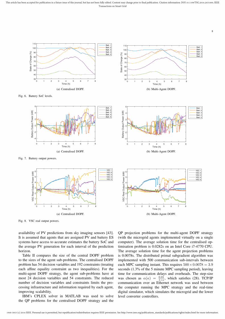
Fig. 6. Battery SoC levels.

Time (h)

0 1 2 3 4 5 6 7 8

Ba

tte

ry O

utp

ut

Po

we

r (k

W)

-4

-2

0

2

4

6Batt. 1

Batt. 2

Batt. 3

Batt. 4

Batt. 5


Time (h)

0 1 2 3 4 5 6 7 8

Ba

tte

ry O

utp

ut

Po

we

r (k

W)

-4

-2

0

2

4

6Batt. 1

Batt. 2

Batt. 3

Batt. 4

Batt. 5


Fig. 7. Battery output powers.

Time (h)

0 1 2 3 4 5 6 7 8

VS

C R

ea

l O

utp

ut

Po

we

r (k

W)

0

1

2

3

4

5

6VSC 1

VSC 2

VSC 3

VSC 4

VSC 5


Time (h)

0 1 2 3 4 5 6 7 8

VS

C R

ea

l O

utp

ut

Po

we

r (k

W)

0

1

2

3

4

5

6VSC 1

VSC 2

VSC 3

VSC 4

VSC 5


Fig. 8. VSC real output powers.

availability of PV predictions from sky imaging sensors [43].

It is assumed that agents that are assigned PV and battery ES

systems have access to accurate estimates the battery SoC and

the average PV generation for each interval of the prediction

horizon.

Table II compares the size of the central DOPF problem

to the sizes of the agent sub-problems. The centralised DOPF

problem has 54 decision variables and 192 constraints (treating

each affine equality constraint as two inequalities). For the

multi-agent DOPF strategy, the agent sub-problems have at

most 24 decision variables and 54 constraints. The reduced

number of decision variables and constraints limits the pro-

cessing infrastructure and information required by each agent,

improving scalability.

IBM’s CPLEX solver in MATLAB was used to solve

the QP problems for the centralised DOPF strategy and the

QP projection problems for the multi-agent DOPF strategy

(with the microgrid agents implemented virtually on a single

computer). The average solution time for the centralised op-

timisation problem is 0.0282s on an Intel Core i7-4770 CPU.

The average solution time for the agent projection problems

is 0.0078s. The distributed primal subgradient algorithm was

implemented with 500 communication sub-intervals between

each MPC sampling instant. This requires 500×0.0078 = 3.9seconds (1.3% of the 5 minute MPC sampling period), leaving

time for communication delays and overheads. The step-size

was chosen as α(κ) = 0.011+κ

, which satisfies (28). TCP/IP

communication over an Ethernet network was used between

the computer running the MPC strategy and the real-time

digital simulator, which simulates the microgrid and the lower

level converter controllers.



9

Time (h)

0 1 2 3 4 5 6 7 8

VS

C R

ea

ctive

Ou

tpu

t P

ow

er

(kV

Ar)

-2

-1.5

-1

-0.5

0

0.5

1

1.5

2VSC 1

VSC 2

VSC 3

VSC 4

VSC 5


Time (h)

0 1 2 3 4 5 6 7 8

VS

C R

ea

ctive

Ou

tpu

t P

ow

er

(kV

Ar)

-2

-1.5

-1

-0.5

0

0.5

1

1.5

2VSC 1

VSC 2

VSC 3

VSC 4

VSC 5


Fig. 9. VSC reactive output powers.

Time (h)

0 1 2 3 4 5 6 7 8

VS

C R

MS

Ou

tpu

t V

olta

ge

(V

pu

)

0.8

0.85

0.9

0.95

1

1.05

1.1

1.15

1.2VSC 1

VSC 2

VSC 3

VSC 4

VSC 5


Time (h)

0 1 2 3 4 5 6 7 8

VS

C R

MS

Ou

tpu

t V

olta

ge

(V

pu

)

0.8

0.85

0.9

0.95

1

1.05

1.1

1.15

1.2VSC 1

VSC 2

VSC 3

VSC 4

VSC 5


Fig. 10. VSC RMS output voltages.

Time (h)

0 1 2 3 4 5 6 7 8

Fre

qu

en

cy (

Hz)

49.99

49.995

50

50.005

50.01VSC 1

VSC 2

VSC 3

VSC 4

VSC 5


Time (h)

0 1 2 3 4 5 6 7 8

Fre

qu

en

cy (

Hz)

49.99

49.995

50

50.005

50.01VSC 1

VSC 2

VSC 3

VSC 4

VSC 5


Fig. 11. VSC output frequencies.

Fig. 5 shows the intermittent generation of the five PV

sources operating under maximum power point tracking.

Under the centralised and multi-agent DOPF strategies,

the VSC output voltage references are updated every 5

minutes, with the goal of minimising power consumption

within power quality and device operating limits. The bat-

teries charge/discharge as required to balance the difference

between the PV generation and the real power exported to the

microgrid. The batteries begin with SoC levels between the

limits of 40% and 100%, as shown in Fig. 6(a) and Fig. 6(b).

The battery output powers for the centralised and multi-agent

DOPF strategies are shown in Fig. 7(a) and Fig. 7(b). Fig. 8(a)

and Fig. 8(b) show the real power exported to the microgrid.

Fig. 9(a) and Fig. 9(b) show the reactive power exported to

the microgrid.

Fig. 6(a) shows that under the centralised DOPF strategy, the

minimum SoC level reached by any of the batteries is 38.9%,

and the maximum SoC is 102.2%. These slight violations

of SoC limits of 40% to 100% are caused by the linear

power flow approximations, and the 5 minute sampling period.

Under the multi-agent DOPF strategy, the limited number of

communication sub-intervals means the central solution is not

fully reached, causing larger SoC constraint violations. As

shown in Fig. 6(b), the SoC levels of the batteries vary between

37.9%, and 102.3%.

Battery utilisation can also be compared using energy

throughput i.e. the total energy discharged from the batteries.

The combined energy throughput of the batteries is 50.85kWh

under the centralised DOPF strategy and 50.67kWh under the

multi-agent DOPF strategy.



10

Under both the centralised and multi-agent DOPF strategies,

the VSC output voltages remain near the lower limit of 0.9pu,

which reduces power consumption since the microgrid load

is primarily resistive. The VSC output voltages are shown in

Fig. 10(a) and Fig. 10(b). Fig. 11(a) and Fig. 11(b) show the

VSC frequencies under the primary droop control strategy.

The multi-agent DOPF strategy provides VSC references

that are further from an exact power balance, causing a

reduction in power quality. This can be quantified in terms

of the mean deviations of the VSC output voltages and

frequencies from their nominal values. The mean VSC output

voltage deviation is 1.66V (0.0040pu) under the centralised

DOPF strategy and 2.64V (0.0064pu) under the multi-agent

DOPF strategy. The mean frequency deviation is 4.8×10−5Hz

under the centralised DOPF strategy and 9.4×10−4Hz under

the multi-agent DOPF strategy.

The multi-agent DOPF strategy also provides slightly sub-

optimal performance in terms of the power consumption min-

imisation objective, but is able to approach the performance

of the centralised optimisation. The average microgrid power

consumption is 15.49kW under the centralised DOPF strategy,

and 15.51kW (0.13% higher) under the multi-agent DOPF

strategy.

VI. CONCLUSION

A multi-agent DOPF strategy has been presented for mi-

crogrids with distributed ES systems. This removes the need

for a central energy management system, providing a scalable

solution for future power networks, which are expected to

include many small distributed renewable sources and ES sys-

tems. The information required by each agent is independent

of the communication network topology, providing increased

flexibility and robustness. The performance of the proposed

control strategy was verified using an RTDS real-time digital

simulator, showing the proper interaction between the multi-

agent MPC implementation and the low level converter con-

trollers.

APPENDIX

Constant power loads can also be included in the static syn-

chronous d-q reference frame voltage-current model. Consider

a load at bus i with real and reactive power components,

Ploadi = vbdiiloaddi + vbqiiloadqi

Qloadi = vbdiiloadqi − vbqiiloaddi (31)

In this case, the load current d-q components are given by,

iloaddi =vbdiPloadi − vbqiQloadi

v2bdi + v2bqi,

iloadqi =vbqiPloadi + vbdiQloadi

v2bdi + v2bqi. (32)

Power flow linearisations are introduced to maintain a convex

formulation of the DOPF problem. Let the d-q components

of the nominal operating voltage at bus i be (Vbdi, Vbqi).

The following affine approximations for the load current d-

q components are obtained.

iloaddi ≈

[

Ploadi(V2bqi − V 2

bdi) + 2QloadiVbdiVbqi

(V 2bdi + V 2

bqi)2

]

vbdi,

+

[

Qloadi(V2bqi − V 2

bdi)− 2PloadiVbdiVbqi

(V 2bdi + V 2

bqi)2

]

vbqi

+2(PloadiVbdi −QloadiVbqi)

(V 2bdi + V 2

bqi)2

. (33)

iloadqi ≈

[

Qloadi(V2bqi − V 2

bdi)− 2PloadiVbdiVbqi

(V 2bdi + V 2

bqi)2

]

vbdi

+

[

Ploadi(V2bdi − V 2

bqi)− 2QloadiVbdiVbqi

(V 2bdi + V 2

bqi)2

]

vbqi

+2(PloadiVbqi +QloadiVbdi)

(V 2bdi + V 2

bqi)2

(34)

The linear functions for the microgrid voltages and currents

from (4) become affine functions of the microgrid bus voltages.

REFERENCES

[1] M. S. Whittingham, “History, Evolution, and Future Status of EnergyStorage,” Proceedings of the IEEE, vol. 100, no. Special CentennialIssue, pp. 1518–1534, May 2012.

[2] R. H. Lasseter, “MicroGrids,” in 2002 IEEE Power Engineering SocietyWinter Meeting. Conference Proceedings (Cat. No.02CH37309), vol. 1,2002, pp. 305–308.

[3] D. E. Olivares, A. Mehrizi-Sani, A. H. Etemadi, C. A. Canizares,R. Iravani, M. Kazerani, A. H. Hajimiragha, O. Gomis-Bellmunt,M. Saeedifard, R. Palma-Behnke, G. A. Jimenez-Estevez, and N. D.Hatziargyriou, “Trends in Microgrid Control,” IEEE Trans. Smart Grid,vol. 5, no. 4, pp. 1905–1919, July 2014.

[4] J. A. Momoh, R. Adapa, and M. E. El-Hawary, “A review of selectedoptimal power flow literature to 1993. I. Nonlinear and quadraticprogramming approaches,” IEEE Trans. Power Syst., vol. 14, no. 1, pp.96–104, Feb. 1999.

[5] Y. Levron, J. M. Guerrero, and Y. Beck, “Optimal Power Flow inMicrogrids With Energy Storage,” IEEE Trans. Power Syst., vol. 28,no. 3, pp. 3226–3234, Aug. 2013.

[6] T. A. Nguyen and M. L. Crow, “Stochastic Optimization of Renewable-Based Microgrid Operation Incorporating Battery Operating Cost,” IEEETrans. Power Syst., vol. PP, no. 99, pp. 1–8, 2015.

[7] D. E. Olivares, C. A. Canizares, and M. Kazerani, “A Centralized EnergyManagement System for Isolated Microgrids,” IEEE Trans. Smart Grid,vol. 5, no. 4, pp. 1864–1875, July 2014.

[8] A. Parisio, E. Rikos, and L. Glielmo, “A Model Predictive ControlApproach to Microgrid Operation Optimization,” IEEE Trans. ControlSyst. Technol., vol. 22, no. 5, pp. 1813–1827, Sept. 2014.

[9] Y. Wang, K. T. Tan, and P. L. So, “Coordinated control of battery energystorage system in a microgrid,” in 2013 IEEE PES Asia-Pacific Powerand Energy Engineering Conference (APPEEC), Dec. 2013, pp. 1–6.

[10] E. Perez, H. Beltran, N. Aparicio, and P. Rodriguez, “Predictive PowerControl for PV Plants With Energy Storage,” IEEE Trans. Sustain.Energy, vol. 4, no. 2, pp. 482–490, Apr. 2013.

[11] E. Mayhorn, K. Kalsi, M. Elizondo, N. Samaan, and K. Butler-Purry,“Optimal control of distributed energy resources using model predictivecontrol,” in 2012 IEEE Power and Energy Society General Meeting, July2012, pp. 1–8.

[12] M. Khalid and A. V. Savkin, “A model predictive control approach tothe problem of wind power smoothing with controlled battery storage,”Renewable Energy, vol. 35, no. 7, pp. 1520–1526, July 2010.

[13] H. Dagdougui, L. Dessaint, and A. Ouammi, “Optimal power exchangesin an interconnected power microgrids based on model predictivecontrol,” 2014 IEEE PES General Meeting — Conference & Exposition,pp. 1–5, July 2014.



11

[14] F. Garcia-Torres and C. Bordons, “Optimal Economical Schedule ofHydrogen-Based Microgrids With Hybrid Storage Using Model Predic-tive Control,” IEEE Trans. Ind. Electron., vol. 62, no. 8, pp. 5195–5207,Aug. 2015.

[15] P. P. Zeng, Z. Wu, X.-P. Zhang, C. Liang, and Y. Zhang, “Modelpredictive control for energy storage systems in a network with highpenetration of renewable energy and limited export capacity,” 2014Power Systems Computation Conference, pp. 1–7, Aug. 2014.

[16] D. J. Hill, T. Liu, and G. Verbic, “Smart grids as distributed learningcontrol,” in 2012 IEEE Power and Energy Society General Meeting, July2012, pp. 1–8.

[17] Y. Simmhan, A. G. Kumbhare, B. Cao, and V. Prasanna, “An Analysisof Security and Privacy Issues in Smart Grid Software Architectureson Clouds,” in 2011 IEEE 4th International Conference on CloudComputing, July 2011, pp. 582–589.

[18] F. L. Lewis, H. Zhang, K. Hengster-Movric, and A. Das, CooperativeControl of Multi-Agent Systems, ser. Communications and ControlEngineering. London: Springer London, 2014.

[19] S. D. J. McArthur, E. M. Davidson, V. M. Catterson, A. L. Dimeas,N. D. Hatziargyriou, F. Ponci, and T. Funabashi, “Multi-Agent Systemsfor Power Engineering Applications-Part I: Concepts, Approaches, andTechnical Challenges,” IEEE Trans. Power Syst., vol. 22, no. 4, pp.1743–1752, Nov. 2007.

[20] A. Bidram, A. Davoudi, F. L. Lewis, and J. M. Guerrero, “DistributedCooperative Secondary Control of Microgrids Using Feedback Lin-earization,” IEEE Trans. Power Syst., vol. 28, no. 3, pp. 3462–3470,Aug. 2013.

[21] J. W. Simpson-Porco, F. Dorfler, and F. Bullo, “Synchronization andpower sharing for droop-controlled inverters in islanded microgrids,”Automatica, vol. 49, no. 9, pp. 2603–2611, Sept. 2013.

[22] V. Nasirian, S. Moayedi, A. Davoudi, and F. L. Lewis, “DistributedCooperative Control of DC Microgrids,” IEEE Trans. Power Electron.,vol. 30, no. 4, pp. 2288–2303, Apr. 2015.

[23] T. Morstyn, B. Hredzak, and V. G. Agelidis, “Distributed CooperativeControl of Microgrid Storage,” IEEE Trans. Power Syst., vol. 30, no. 5,pp. 2780–2789, Sept. 2015.

[24] T. Morstyn, B. Hredzak, and V. G. Agelidis, “Cooperative Multi-Agent Control of Heterogeneous Storage Devices Distributed in a DCMicrogrid,” IEEE Trans. Power Syst., vol. 31, no. 4, pp. 2974–2986,Sept. 2015.

[25] T. Morstyn, B. Hredzak, G. D. Demetriades, and V. G. Agelidis, “UnifiedDistributed Control for DC Microgrid Operating Modes,” IEEE Trans.Power Syst., vol. 31, no. 1, pp. 802–812, Jan. 2016.

[26] C. Li, T. Dragicevic, M. G. Plaza, F. Andrade, J. C. Vasquez, andJ. M. Guerrero, “Multiagent based distributed control for state-of-chargebalance of distributed energy storage in DC microgrids,” in IECON 2014- 40th Annual Conference of the IEEE Industrial Electronics Society,Oct. 2014, pp. 2180–2184.

[27] C. Li, T. Dragicevic, J. C. Vasquez, J. M. Guerrero, and E. A. A.Coelho, “Multi-agent-based distributed state of charge balancing controlfor distributed energy storage units in AC microgrids,” in 2015 IEEEApplied Power Electronics Conference and Exposition (APEC), Mar.2015, pp. 2967–2973.

[28] W. Shi, X. Xie, C.-c. Chu, and R. Gadh, “A distributed optimalenergy management strategy for microgrids,” in 2014 IEEE InternationalConference on Smart Grid Communications (SmartGridComm), vol. 6,no. 3, Nov. 2014, pp. 200–205.

[29] A. Cortes and S. Martınez, “On distributed reactive power and storagecontrol on microgrids,” International Journal of Robust and NonlinearControl, Jan. 2016.

[30] M. Kraning, E. Chu, J. Lavaei, and S. Boyd, “Dynamic Network EnergyManagement via Proximal Message Passing,” Foundations and Trendsin Optimization, vol. 1, no. 2, pp. 70–122, Nov. 2014.

[31] G. Hug, S. Kar, and C. Wu, “Consensus+Innovations Approach forDistributed Multiagent Coordination in a Microgrid,” IEEE Trans. SmartGrid, vol. 6, no. 4, pp. 1893–1903, July 2015.

[32] S. Papathanassiou, N. Hatziargyriou, and K. Strunz, “A Benchmark LowVoltage Microgrid Network,” Proceedings of the CIGRE Symposium:Power Systems with Dispersed Generation, pp. 1–8, Apr. 2005.

[33] N. Pogaku, M. Prodanovic, and T. C. Green, “Modeling, Analysis andTesting of Autonomous Operation of an Inverter-Based Microgrid,”IEEE Trans. Power Electron., vol. 22, no. 2, pp. 613–625, Mar. 2007.

[34] Zhu, M. and S. Martinez, “On Distributed Convex Optimization UnderInequality and Equality Constraints,” IEEE Trans. Autom. Control,vol. 57, no. 1, pp. 151–164, Jan. 2012.

[35] M. Diaz-Aguilo, J. Sandraz, R. Macwan, F. de Leon, D. Czarkowski,C. Comack, and D. Wang, “Field-validated load model for the analysis

of CVR in distribution secondary networks: Energy conservation,” IEEETrans. Power Del., vol. 28, no. 4, pp. 2428–2436, Oct. 2013.

[36] Z. Wang, M. Begovic, and J. Wang, “Analysis of conservation voltagereduction effects based on multistage SVR and stochastic process,” IEEETrans. Smart Grid, vol. 5, no. 1, pp. 431–439, Jan. 2014.

[37] Z. Wang and J. Wang, “Review on implementation and assessment ofconservation voltage reduction,” IEEE Trans. Power Syst., vol. 29, no. 3,pp. 1306–1315, May 2014.

[38] Z. Wang and J. Wang, “Time-varying stochastic assessment of conser-vation voltage reduction based on load modeling,” IEEE Trans. PowerSyst., vol. 29, no. 5, pp. 2321–2328, Sept. 2014.

[39] Z. Wang, B. Chen, J. Wang, and M. M. Begovic, “Stochastic DGPlacement for Conservation Voltage Reduction Based on Multiple Repli-cations Procedure,” IEEE Trans. Power Del., vol. 30, no. 3, pp. 1039–1047, June 2015.

[40] B. Zhao, X. Zhang, J. Chen, C. Wang, and L. Guo, “Operation opti-mization of standalone microgrids considering lifetime characteristicsof battery energy storage system,” IEEE Trans. Sustain. Energy, vol. 4,no. 4, pp. 934–943, 2013.

[41] R. Dufo-Lopez, J. M. Lujano-Rojas, and J. L. Bernal-Agustın, “Com-parison of different lead-acid battery lifetime prediction models for usein simulation of stand-alone photovoltaic systems,” Applied Energy, vol.115, pp. 242–253, Feb. 2014.

[42] T. Kim and W. Qiao, “A Hybrid Battery Model Capable of CapturingDynamic Circuit Characteristics and Nonlinear Capacity Effects,” IEEETrans. Energy Convers., vol. 26, no. 4, pp. 1172–1180, Dec. 2011.

[43] M. Diagne, M. David, P. Lauret, J. Boland, and N. Schmutz, “Reviewof solar irradiance forecasting methods and a proposition for small-scaleinsular grids,” Renewable and Sustainable Energy Reviews, vol. 27, pp.65–76, Nov. 2013.

Thomas Morstyn (S’13) received the B.E. (Hon.)degree in electrical engineering from the Universityof Melbourne, Australia, in 2011.

He worked as an electrical engineer in the RioTinto Technology and Innovation group for twoyears. He is currently working towards the Ph.D. de-gree at the Australian Energy Research Institute, TheUniversity of New South Wales, Sydney, NSW, Aus-tralia. His current research interests include multi-agent control and optimisation for the integration ofdistributed renewable generation and energy storage

systems into power networks.

Branislav Hredzak (M’98-SM’13) received theB.Sc./M.Sc. degree from the Technical Universityof Kosice, Slovak Republic, in 1993, and the Ph.D.degree from Napier University of Edinburgh, U.K.,in 1997, all in electrical engineering.

He was a Lecturer and a Senior Researcher in Sin-gapore from 1997 to 2007. He is currently a SeniorLecturer in the School of Electrical Engineering andTelecommunications, The University of New SouthWales, Sydney, NSW, Australia. His current researchinterests include hybrid storage technologies and

advanced control systems for power electronics and storage systems.

Vassilios G. Agelidis (S’89-M’91-SM’00-F’16) wasborn in Serres, Greece. He received the B.Eng.degree in electrical engineering from the DemocritusUniversity of Thrace, Thrace, Greece, in 1988, theM.S. degree in applied science from ConcordiaUniversity, Montreal, QC, Canada, in 1992, and thePh.D. degree in electrical engineering from CurtinUniversity, Perth, Australia, in 1997. He has workedat Curtin University (1993–1999), University ofGlasgow, U.K. (2000–2004), Murdoch University,Perth, Australia (2005–2006), the University of Syd-

ney, Australia (2007–2010), and the University of New South Wales (UNSW),Sydney, Australia (2010–2016). He is currently a professor at the Departmentof Electrical Engineering, Technical University of Denmark.

Dr. Agelidis received the Advanced Research Fellowship from the U.K.’sEngineering and Physical Sciences Research Council in 2004. He was theVice-President Operations within the IEEE Power Electronics Society from2006 to 2007. He was an AdCom Member of the IEEE Power ElectronicsSociety from 2007 to 2009 and the Technical Chair of the 39th IEEE PowerElectronics Specialists Conference, Rhodes, Greece, 2008.

network topology independent multi-agent dynamic optimal

Documents