Existence and continuity of optimal solutions to some

structural topology optimization problems including

unilateral constraints and stochastic loads∗

Michael Patriksson† and Joakim Petersson‡

September 26, 2001

Abstract

We consider a general discrete structural optimization problem including unilateral con-straints arising from, for example, non-penetration conditions in contact mechanics or non-compression conditions for elastic ropes. The loads applied (and, in principle, also other datasuch as the initial distances to the supports), are allowed to be stochastic, which we handlethrough a discretization of the probability space. The existence of optimal solutions to theresulting problem is established, as well as the continuity properties of the equilibrium dis-placements and forces with respect to the lower bounds on the design variables. The latterfeature is important in topology optimization, in which one includes the possibility of vanishingstructural parts by setting design variable values to zero. In design optimization computa-tions, one usually replaces the zero lower design bound by a strictly positive number, hencerewriting the problem into a sizing form. For several such perturbations, we prove that theglobal optimal designs and equilibrium states converge to the correct ones as the lower boundconverges to zero.

1 Introduction

1.1 Motivation

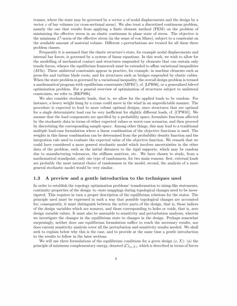
Topology optimization of mechanical structures refers to the subfield of structural optimizationwhere parts of the design region are allowed to be occupied by a varying amount of solid material,including no material at all. This means that the sets of admissible designs and the correspondingstructural responses are very large. On the one hand, some designs might result in a structure thatcannot carry the applied load at all, while, on the other hand, some designs carry the particularload very efficiently. The distinction between sizing and topology optimization is usually that inthe latter the amount of material, for example, a thickness or cross-sectional area, is allowed to bezero. Figure 1 shows a simple one-dimensional structure1 that consists of a bar suspended with onecable. Suppose that one has chosen the bar material volume (or the cross-sectional area) x and thecable material volume X to be design variables. If the objective is to maximize the displacement

∗This research is supported by a grant from the Swedish Research Council for Engineering Sciences (grant TFR98-125), which is greatfully acknowledged.

†Department of Mathematics, Chalmers University of Technology, SE-412 96 Goteborg, Sweden. Email: mi-pat@math.chalmers.se

‡Department of Mechanical Engineering, Mechanical Engineering Systems, Linkoping University, SE-581 83Linkoping, Sweden. Email: joape@ikp.liu.se

1This example will be studied in more detail in Section 3.1.2.

1

x

f

σ =1/2 σ =12 1

11

X

Figure 1: The cable suspended one-bar truss.

in the middle, then there are in fact no optimal solutions in the topology optimization problemunlike in the corresponding sizing optimization problem. The reason is that the objective valuecan be made arbitrarily large by choosing x and X arbitrarily close to zero (which is not allowedin the sizing case). Although the objective function is somewhat artificial, similar phenomena canoccur also in a more natural context, and it illustrates that it is in general not obvious that thereexist solutions to topology optimization problems as some mathematical properties are differentfrom the sizing case. In this example, the key issue can be described by a lack of closedness of thefeasible set (in the problem statement involving both the state and design variables), which hasbeen observed earlier to be an important factor in establishing existence of solutions in generalmathematical programs with equilibrium constraints in, e.g., [LPR96, Section 1.4].

Sizing problems are typically easier than topology optimization problems for more reasons thanthat the existence issue is easier—for instance the design sensitivities, that is, the derivatives ofthe state variables (in the nested version of the problem) with respect to changes in design, areharder to determine in other problem types such as in shape optimization. Therefore, if topologyoptimization problems could be cast into a sizing-like problem statement, then the problem wouldbe much easier to handle, since design sensitivities and unique equilibrium solutions always existand are computable. The traditional way to restate or modify the problem statement from atopology optimization problem to a sizing-like statement is here referred to as an ε-perturbation(or, an ε-relaxation). In order for the ε-perturbation to be valid, the solution sets of the restatedsizing-like problems should be close to those of the original problem statement for small parametervalues ε. Difficulties in finding and validating proper ε-perturbations should somehow be expectedsince the unperturbed problem statements include many different structural topologies whereasthe sizing problems cover only one.

The most common ε-perturbation is to replace the design zero lower bounds by a small posi-tive number ε—a perturbation which is valid for some minimum compliance problems (see, e.g.,[Ach98]). Concerning stress-constrained minimum weight problems, however, the situation is morecomplicated. Consider again the simple structure in Figure 1, and suppose that one wants, morenaturally, to minimize the total weight subject to the stress constraints shown in the figure.2 Thebar can sustain any stress with magnitude less than or equal to σ1 (specific for the bar material),while the cable can sustain no compressive stresses and no tensile stresses exceeding σ2 (specific

2This example will be studied in more detail in Section 4.2.4.

2

x

x

2

1

x + x = 2x + x = 112 21

constant weight

2

X

1

x

constant weight

2

1

x+X=1 x+X=2

Figure 2: The admissible design domain. The optimal solution is at the black circle.

for the cable material). Figure 2 shows the feasible domain for the design variables (x, X) afterthe state variables have been eliminated. Note that this domain consists of the union of a two-dimensional, convex domain and a one-dimensional ”spike” appended to it. As seen in the figure,the optimal design is located on the spike, and simply enforcing small strictly positive lower boundson x and X will obviously change the feasible set in a discontinuous fashion; no matter how smalllower design bound one uses, the distance to the desired optimal design will always be at least1/

√2.Observations of this kind were done by Sved and Ginos as early as in 1968 [SvG68]. The

problem is sometimes referred to as the ”stress singularity phenomenon” or ”singular topologies”,cf., e.g., [Kir90, Roz01]. Two different perturbations which include ε-terms in the stress constraintswere introduced by Svanberg [Sva94] and Cheng and Guo [ChG97]. Since it is of paramountimportance to know if, and for which type of ε-perturbation, the restated sizing-like problem’sdesign solutions converge to the set of optimal designs in the original problem statement as theparameter ε approaches zero, it is the main theme of this paper to prove such continuity results,as well as the existence of optimal solutions, for several different problem classes. When justifyingcorrect ε-perturbations the proofs rely heavily on the continuity properties of the mappings thatprovide the set of equilibrium states for given designs, including changes in the connectedness ofthe mechanical structure. These continuity results are interesting in their own right, and based ontheir generality we believe them to be useful also for applications other than those covered here.

We do not directly aim at providing methods for finding optimal solutions to the problemsstudied, but focus on justifying the optimization statements. Having proven that some sizing-likeproblem’s optimal solutions are close to the desired ones, one can usually rely on the fact that thenested versions of sizing problems are often successfully solved by sequential convex or separableprogramming algorithms in conjunction with standard sensitivity analysis.

1.2 Scope

Two of the most natural and classical structural optimization problems are minimum compliance,or, equivalently, maximum stiffness, under a volume constraint, and minimum weight under stressconstraints. We consider these problem classes in a discrete framework, that is, we assume that thestate and design are specified by a finite number of variables, which is the case for example with

3

trusses, where the state may be governed by a vector u of nodal displacements and the design by avector x of bar volumes (or cross-sectional areas). We also treat a discretized continuous problem,namely the one that results from applying a finite element method (FEM) on the problem ofminimizing the effective stress in an elastic continuum in plane state of stress. The objective isthe minimum L2-norm of the effective stress (in the sense of von Mises), subject to a constraint onthe available amount of material volume. Different ε-perturbations are treated for all these threeproblem classes.

Frequently it is assumed that the elastic structure’s state, for example nodal displacements andinternal bar forces, is governed by a system of linear equations. In this work, we wish to allow forthe modelling of mechanical contact and structures suspended by elements that can sustain onlytensile forces, whence the equilibrium framework must be extended to affine variational inequalities(AVIs). These unilateral constraints appear in practice, for example, in machine elements such aspress-fits and turbine blade roots, and for structures such as bridges suspended by elastic cables.When the state problem is governed by a variational inequality, the overall design problem is termeda mathematical program with equilibrium constraints (MPEC), cf. [LPR96], or a generalized bileveloptimization problem. For a general overview of optimization of structures subject to unilateralconstraints, we refer to [HKP99b].

We also consider stochastic loads, that is, we allow for the applied loads to be random. Forinstance, a heavy weight hung by a crane could move in the wind in an unpredictable manner. Theprocedure is expected to lead to more robust optimal designs, since structures that are optimalfor a single deterministic load can be very inefficient for slightly different loads, cf. [CPW01]. Weassume that the load components are specified by a probability space, formulate functions affectedby the stochastic data in terms of either expected values or worst-case scenarios, and then proceedby discretizing the corresponding sample space. Among other things, this may lead to a traditionalmultiple load-case formulation where a linear combination of the objective functions is used. Theweights in this linear combination can be determined from the probability density function and theintegration rule used to evaluate the expected value of the objective function. We remark that wecould have considered a more general stochastic model which involves uncertainties in the otherdata of the problem, such as the initial distances to the rigid supports, which may be randomdue to manufacturing tolerances, the stiffness matrices, etc. We have chosen to study, from amathematical standpoint, only one type of randomness, for two main reasons: first, external loadsare probably the most natural choice of randomness in the model; second, the analysis of a moregeneral stochastic model would be very similar.

1.3 A preview and a gentle introduction to the techniques used

In order to establish the topology optimization problems’ transformation to sizing-like statements,continuity properties of the design–to–state mappings during topological changes need to be inves-tigated. This requires in turn a proper description of the equilibrium relations for the states. Theprinciple used must be expressed in such a way that possible topological changes are accountedfor; consequently, it must distinguish between the active parts of the design, that is, those indicesof the design variables which are nonzero, and those corresponding to holes or voids, that is, zerodesign variable values. It must also be amenable to sensitivity and perturbation analyses, whereinwe investigate the changes in the equilibrium state to changes in the design. Perhaps somewhatsurprisingly, neither does one equilibrium formulation suffice to reach the necessary results, nordoes current sensitivity analysis cover all the perturbation and sensitivity results needed. We shallseek to explain below why this is the case, and to provide at the same time a gentle introductionto the results to follow in the later sections.

We will use three formulations of the equilibrium conditions for a given design (x, X): (a) theprinciple of minimum complementary energy, denoted (C)(x,X), which is described in terms of forces

4

only; (b) the principle of minimum potential energy, denoted (P)(x,X), which is described in termsof displacements only; and (c) an AVI which is described in terms of forces and displacementssimultaneously. The two first problems form, for a given design (x, X), a primal–dual pair ofquadratic programs, whose optimality conditions are exactly the AVI.

To each of these three formulations corresponds a main result on the continuity of the design–to–state mapping. The first states that, given any convergent sequence of designs, and assuming theelastic energy remains bounded, the limit design possesses a state of equilibrium and the sequenceof equilibrium forces converges to the limit design’s equilibrium force (Theorem 3.1). (This ishowever not the case when the equilibrium principle is formulated in the displacement space.) Theproof of the result utilizes the lower semicontinuity property of the extended real-valued energyfunction E , and the formulation (C)(x,X). The other two continuity results are less general, asthey are stated for particular design sequences where each element in the design vector decreasesstrictly monotonically to a fixed design variable value (and which vector is assumed to have a statein equilibrium). The total potential energy principle (P)(x,X) is in Theorem 3.2 utilized to establishthat the sequence of displacements converges to the least-energy displacement among all possibleequilibrium displacements. This is the only result presented which has been analyzed previously;it is in fact a special case of the perturbation technique known as the regularization of a nonstrictlyconvex program (e.g., [Bro66]); for this special caes, we felt however that an independent proofwould be illustrative. The Theorems 3.3 and 3.4, finally, utilize the AVI formulation. The firstresult establishes that the convergence rate of the equilibria is at least linear. The proof is basedon the recent development of the theory of error bounds for the solutions to AVIs and systems oflinear inequalities, and on Theorem 3.2. The second result establishes that in the region where thedesign is strictly positive, the state is locally Lipschitz continuous in the design.

The design–to–state mapping is somewhat special, and in fact it is less ”continuous” thanwhat current sensitivity analysis presumes. The obstacle is the effect of changes in the topology.As the set of active indices in the design changes, the quadratic programs corresponding to thetwo equilibrium principles will have different numbers of constraints, in which case the feasiblesets are not lower semicontinuous [the case of (C)(x,X)], or the dimension of the null space of theobjective’s Hessian changes [the case of (P)(x,X)]. (Sensitivity results are normally not formulatedsuch that the number of constraints or dimension of the null space of a matrix are allowed todiffer.) In an equivalent reformulation of (C)(x,X), the number of constraints is constant, but theobjective is instead extended real-valued, with infinite values whenever a force is nonzero in aninactive design element. Although the energy functional is lower semicontinuous (lsc), it is notcontinuous at an equilibrium as it is not upper semicontinuous, which, again, precludes the useof existing analysis, such as Theorem 4.3.3 in [BGK+83]. (Present quantitative characterizationsof continuity, e.g., upper- and lower-semicontinuity results, all require at least continuity of theobjective function near the ”reference point” jointly in the problem variables and parameters. Itseems rather unlikely to be able to obtain a result applicable to a general class of optimizationproblems without this requirement. What helps us to be able to reach the sensitivity results soughtare, in short, the favourable properties of the lsc function (x, y) 7→ x2/y on R×R+, and the recenttheory of error bounds for the solutions to AVIs.) The complementary energy problem’s optimalsolution is unique if a feasible solution exists. Restricted to a set where the energy is bounded, thedesign–to–force mapping is closed. The total potential energy principle can however in general havean unbounded solution set, due to the singularity of the stiffness matrix when some design variablesare zero; further, the rank of this matrix changes dramatically with the index set of active designvariables. To a sequence of equilibrium forces may correspond a divergent sequence of equilibriumdisplacements, if the limit design corresponds to a singular stiffness matrix. Thus, the design–to–displacement mapping is not closed. The two quadratic programs are hence not amenable totraditional sensitivity analysis. The AVI is constructed such that a constraint enforces an inactivedesign element to have a zero force, so the problem is in some ways better posed. On the other

5

hand, the sensitivity analysis of AVIs is weaker than for quadratic programs: the sensitivity analysisavailable is only local, unless the limit design is strictly positive, and can not be used to establishthe existence of an equilibrium for a limit design.

Each of the three continuity results is applied in the results which then follow in Sections 4 and5, which are devoted to cable suspended trusses and finite element discretized sheets in contact,respectively. For each problem, we analyze the existence of optimal designs, and correct formsof ε-perturbation, for two problem statements: minimum compliance given a limited amount ofmaterial, and stress-constrained minimum weight. The compliance minimization problem is theeasiest by far; the proofs use the design–to–force mapping’s continuity as the main ingredient.The straightforward ε-perturbation mentioned earlier is sufficient, and the optimal design problemcan be given several convex, or convex–concave, optimization formulations. The stress-constrainedminimum weight problem is the most difficult. Existence relies on using design–to–force continuity;in the perturbation results, also the rate of convergence is needed, and in addition to setting thelower design bound to ε, we must introduce a term which converges to zero—faster than ε but slowerthan ε2—into the stress constraints. The problem where the effective stress in an elastic continuumis minimized is in character somewhat ”in between” the other two problems in difficulty. Besidesthe design–to–force continuity, the displacements’ convergence to the least-energy displacement isutilized. These results make it all the more clear that each of the three equilibrium principlesstudied have an important role to play.

To summarize, the rest of the paper is organized as follows. Section 2 deals with the threeprinciples of equilibrium: minimum of complementary energy, minimum total potential energy,and an AVI expressed in all state variables simultaneously. Section 3 states and proves severalpropositions on the continuity properties of the state variables with respect to changes in thedesign variables, including changes in topology. The following two sections deal with interestinginstances of structural optimization problems. Section 4 accounts for cable suspended trusses,minimum compliance as well as stress constrained minimum weight. Section 5 treats the FE-discretized sheet problem where the L2-norm of the effective stress is minimized. Finally, Section6 includes some remarks and comments on interesting further research.

2 The equilibrium problem

The structure is assumed to consist of at most m parts such as bars or finite elements. The materialvolume allocated at part i is described by xi, i = 1, . . . , m. Clearly, xi ≥ 0 holds, and xi = 0 isinterpreted as a structural void. We denote the set of present (or, active) parts of the structure bythe index set

I(x) := i | xi > 0 ⊆ 1, . . . , m.

The structure is further assumed to consist of nodes, the displacements of which are collected ina (column) vector u ∈ R

n (note: prescribed zero-displacements are removed). The deformation ofeach (present) part is described by sc strain components, collected in a vector εi for i = 1, . . . , m.This strain is connected to the displacement through the relation

εi = Biu, i ∈ I(x), (1)

where Bi ∈ Rsc×n is a kinematic transformation matrix. The stress state of each present part is

described by σi ∈ Rsc, and is assumed to be related to the strain according to Hooke’s generalized

law:

σi = Eεi, i ∈ I(x), (2)

6

where E ∈ Rsc×sc is the symmetric and positive definite matrix of elasticity constants. We define

the force-like variable si as

si = xiσi, i ∈ I(x), (3)

which in fact has unit (force × length). (For a bar it is simply the bar force times the bar length.)We set Di(x) = xiE, and then (1)–(3) give

si = Di(x)Biu, i ∈ I(x). (4)

External forces (including forces due to unilateral contact and cables) are represented by a vectorF ∈ R

n; static force equilibrium is governed by

F =∑

i∈I(x)

BTi si. (5)

Note that, if we define the structural stiffness matrix as

K(x) =

m∑

i=1

xiBTi EBi, (6)

then (4) and (5) yield

F = K(x)u. (7)

We assume that there are sufficiently many prescribed zero-displacements for K(1m) to be positivedefinite. (Here, 1m denotes the m-vector of ones.)

2.1 Special case 1: Linear triangular finite elements

In this particular case, we consider a plane structure, sc = 3 and strains εi = (εx, εy, γxy)T , stresses

σi = (σx, σy , τxy)T , and, assuming plane stress and an isotropic elastic body,

E =E0

1 − ν2

1 ν 0ν 1 00 0 1−ν

2

,

where ν ∈ (−1, 1/2) is Poisson’s ratio and E0 > 0 is Young’s modulus. Let the set ηi contain thenode numbers for the nodes belonging to element i. If we define matrices

BA =

∂NA

∂x10

0 ∂NA

∂x2∂NA

∂x2

∂NA

∂x1

,

where NA are shape functions, then the Bi’s are constructed so that

εi =∑

A∈ηi

BAuA = Biu,

where uA ∈ R2 is the displacement at node A.

Based on the different stress components in a finite element one can calculate a single effectivestress according to

σei =

√σT

i Mσi,

7

where, in the case of von Mises effective stress,

M =

1 − 1

2 0− 1

2 1 00 0 3

.

2.2 Special case 2: Truss structures

This particular case involves a set of bars in one, two or three dimensions. We have sc = 1, σi issimply the stress in the bar, and εi the strain. The matrix E is Young’s modulus of the bar, and

Di = xiE, si = xiσi.

Hence, si is the bar force times its length, Bi is 1/LiγTi , where Li is the bar’s length, and γi

contains the bar’s direction cosines.The effective stress in a bar is the absolute value of the single stress value; hence, σe

i =√σT

i Mσi = |σi| holds, where here M = 1 holds.

2.3 The unilateral constraints

Suppose we have unilateral rigid supports that cannot be penetrated by the nodes of the structure.Then, these unilateral constraints can be formulated as

C1u ≤ g1, (8)

where C1 ∈ Rr1×n is a kinematic transformation matrix, and g1 ∈ R

r1 is the vector of the initialgaps. If we let λ ∈ R

r1 be the vector of contact forces, then the relations

λ ≥ 0, λT (C1u − g1) = 0 (9)

reflect the facts that the contact is non-adhesive and that contact forces do not develop at adistance. We shall assume that each node is subject to not more than one contact condition(or, more generally, that if there are more than one contact condition for one node then theyare orthogonal), whence C1C

T1 equals the r1 × r1 identity matrix. (We refer to this as C1 being

quasi-orthogonal.)Suppose now also that there are at most r2 cables (or, ropes), the ends of which are attached to

nodes of the structure and (possibly) also suspended at rigid foundations. The jth cable’s volumeis denoted by Xj, and similarly to I(x) we define

J (X) := j | Xj > 0 ⊆ 1, . . . , r2.

We let ej be the cable’s elongation, (g2)j its initial slack, and Sj its tensile force. Then, thebehavior of the cables can be described by

γTj u − ej − (g2)j ≤ 0, Sj ≥ 0, (γT

j u − ej − (g2)j)Sj = 0, j ∈ J (X), (10)

where γj is a vector which contains the unit vector of cable j (in the same way as for a bar element).The cables’ stiffness constants are

kj(X) =XjEc

L2j

, j ∈ J (X), (11)

8

where Ec > 0 is Young’s modulus for the cable material and Lj > 0 the cable lengths. Therefore,the cable elasticity is modelled by

Sj = kj(X)ej , j ∈ J (X), (12)

(and hence Sj ≥ 0 if and only if ej ≥ 0). We interpret (10) and (12) as follows: if Sj = 0, thenby (12), ej = 0, and what is left of (10) is γT

j u ≤ (g2)j which asserts that the elongation of thestraight line between the cable’s end points cannot exceed the initial slack. If, on the other hand,Sj > 0, then (10) states that γT

j u − ej = (g2)j , that is, the cable elongation equals the elongationof the straight line between the cable’s end points minus the initial slack.

The cable forces are directed along the direction of the cables, defined through the vectorγj ; we presume frictionless contact, whence the directions of contact forces are known (namelyorthogonally to the unilateral supports). Hence, if f ∈ R

n denotes external prescribed forces(different from cable and contact forces), static equilibrium [see (5)] is governed by

CT1 λ +

∑

i∈I(x)

BTi si +

∑

j∈J (X)

Sjγj = f, (13)

since

F = f − CT1 λ −

∑

j∈J (X)

Sjγj .

Given a structure and cable design (x, X), the overall equilibrium problem can now be sum-marized as follows: For all i ∈ I(x) and j ∈ J (X), find nodal displacements u, cable elongationsej , contact forces λ, cable forces Sj and internal structure forces si such that (4), (8)–(10), and(12)–(13) hold.

2.4 Energy principles

2.4.1 Minimum complementary energy

The principle of minimum of complementary energy states that among all force distributions thatsatisfy static force equilibrium [that is, (5)], the one present in equilibrium (if any), is one whichminimizes the elastic energy of the structure. In parts of the structure where xi = 0 or Xj = 0holds, elastic energy cannot be stored. Using the notation I(x) and J (X) for positive elementsxi and Xj, respectively, and sI(x) and SJ (X) for the corresponding sub-vectors, we can then statethe elastic energy minimization problem as follows:

(C)(x,X)

min(sI(x),SJ (X),λ)

EI,J (x, X, s, S, λ) :=1

2

∑

i∈I(x)

sTi E−1si

xi+ gT

1 λ

+∑

j∈J (X)

((LjSj)

2

2EcXj+ (g2)jSj

),

s.t.

CT1 λ +

∑

i∈I(x)

BTi si +

∑

j∈J (X)

Sjγj = f,

λ≥0,

SJ (X) ≥0.

In the below result, we use the notions that a real-valued function, say ϕ : Rn 7→ R ∪ +∞,

is coercive (with respect to a set Y ) if Y is bounded or lim‖xt‖→∞, xt∈Y ϕ(xt) = ∞, and that ϕ islower semicontinuous (lsc) if for any x ∈ R

n, lim infy→x ϕ(y) ≥ ϕ(x).

9

Theorem 2.1 (Existence of optimal solutions to (C)(x,X)). Suppose the feasible set of the problem(C)(x,X) is nonempty. Then, there exists a unique optimal solution to the problem (C)(x,X).

Proof. The objective function of (C)(x,X) is coercive and lsc. The former follows for (sI(x), SJ (X))immediately, and for λ we note that by the quasi-orthogonality of C1, λ is uniquely determinedby them. Lower semicontinuity follows from continuity. Since EI,J is strictly convex in thosevariables, also uniqueness follows.

We investigate the optimality conditions for this problem. We introduce u as the Lagrangemultipliers for the equality constraints. The stationarity conditions for the Lagrangian then becomethe following: stationarity with respect to s gives (4); through the definition (11) we derive (10)and (12) as the stationarity conditions with respect to S ≥ 0; stationarity with respect to λ ≥ 0yields (8) and (9); finally, stationarity with respect to u of course gives us (13). Summarizing, then,the conditions which characterize the minimal complementary energy are precisely the conditions(4), (8)–(10), and (12)–(13), discussed from a mechanical standpoint in the previous section.

2.4.2 Minimum total potential energy

We will next state and investigate a principle of minimum potential energy. Given a design (x, X)the problem is the following:

(P)(x,X)

min(u,eJ (X))

1

2

∑

i∈I(x)

xiuT BT

i EBiu +1

2

∑

j∈J (X)

EcXj

L2j

e2j − fT u,

s.t.

C1u≤ g1,

γTj u − ej ≤ (g2)j , j ∈ J (X).

Investigating its optimality conditions, we introduce λ ≥ 0 and Sj ≥ 0, j ∈ J (X), as theLagrange multipliers for the inequality constraints. Pursuing, as for the problem (C)(x,X), thestationarity conditions for the resulting Lagrangian reformulation, we obtain the following. Wefirst note that although s does not enter into this problem, we will use (4) as its definition. Then,stationarity with respect to u yields (13); stationarity with respect to e gives (12); stationaritywith respect to λ ≥ 0 gives (8) and (9); finally, stationarity with respect to S ≥ 0 gives (10). So,to summarize, the characterization of the minimum potential energy is, again, the conditions (4),(8)–(10), and (12)–(13), discussed from a mechanical standpoint in the previous section.

This development also establishes that the problems (C)(x,X) and (P)(x,X) constitute equivalent,primal–dual pairs of convex quadratic programs, since they have the same optimality conditions.This means that if there exists an optimal solution to (C)(x,X), then there are optimal solutionsto (P)(x,X), and, conversely, if there is at least one optimal solution to (P)(x,X), then (C)(x,X) isuniquely solvable.

In the optimal solution to these problems, the values of the variables sI\I(x) and (S, e)J\J (X)

are unspecified. (This is a direct effect of the way in which the primal–dual pair of equilibriumproblems were stated, as these variables are not present in their formulations or in their Lagrangian-based optimality conditions.) This is, however, a drawback when we want to consider existence,continuity and other sensitivity issues for varying values of (x, X) [and consequently for varyingindex sets I(x) and J (X)], in particular as a subset of their elements tend to zero. In order to statea complete set of equilibrium conditions, containing all the variables, we shall next formulate anaffine variational inequality problem which embraces the conditions (4), (8)–(10), and (12)–(13).The idea is to introduce the conditions (4) and (12) explicitly into the formulation, for the entiresets of variables, and not just for the index sets I(x) and J (X), whereby we explicitly account for

10

the active parts of the structure by forcing zero elements in (x, X) to correspond to zero elementsin (s, S). Mechanically speaking, the only possible force in a void is zero.

2.4.3 Equilibrium characterization as an affine variational inequality

Let Q be a matrix in Rp×p, q a vector in R

p and Y a polyhedral subset of Rp. The affine variational

inequality (AVI) problem associated with this data is to find y∗ ∈ Y such that

[Qy∗ + q]T (y − y∗) ≥ 0, y ∈ Y. (14)

(In case Q is symmetric, this variational inequality constitutes the necessary conditions for y∗ tobe a local minimum point of the function y 7→ 1

2yT Qy + qT y over the set Y .) We denote thisproblem by AVI (q, Q, Y ).

We now state the equilibrium conditions for forces and displacements as an AVI. To this end,we first define C2 as the r2 × n matrix of the vectors γj , B as the (m · sc) × n matrix created bystacking the matrices Bi on top of each other, s as the m ·sc vector created by stacking the vectorssi on top of each other, D(x) as the (m ·sc)× (m ·sc) block-diagonal matrix created by placing thematrices Di(x) along the diagonal, and, finally, k(X) as the r2 × r2 diagonal matrix with diagonalelements kj(X). Let

y :=

uesSλ

, Q :=

0 0 BT CT2 CT

1

D(x)B 0 −I 0 00 k(X) 0 −I 0

−C2 I 0 0 0−C1 0 0 0 0

, and q :=

−f00g2

g1

, (15)

and Y := Rn ×R

r2 × Rm·sc × R

r2+ ×R

r1+ . (Note: R+ denotes the set of nonnegative reals, whereas

R++, to be used later, denotes the set of strictly positive reals.)It is easy to check that the AVI with this data is a statement of the conditions (13), (4), (12),

(10), (8), (9), in that order, where now the conditions are stated over all the variables.For the AVI given by (14), (15) we next establish an elementary result on the closedness property

of its solution set when viewing (x, X) as parameters. To this end, we shall introduce the newnotation AVI (q, Q(x, X), Y ) and SOL (q, Q(x, X), Y ) to denote the AVI problem (14), (15) and itssolution set for a given pair (x, X).

Theorem 2.2 (Closedness of the mapping (x, X) 7→ SOL(q, Q(x, X), Y )). The mapping (x, X) 7→SOL(q, Q(x, X), Y ) is closed on R

m × Rr2 .

Proof. Consider a sequence Rm × R

r2 ⊃ (xt, Xt) → (x∗, X∗), and an arbitrary sequence ytfulfilling yt ∈ SOL(q, Q(xt, Xt), Y ) for all t. Suppose that the latter sequence has a limit point,y∗. Closedness amounts to having y∗ ∈ SOL(q, Q(x∗, X∗), Y ). In order to establish this inclusion,consider, for a fixed vector y ∈ Y in the AVI given by (14), (15), the sequence of solutions over t.Then, noting that Q(·, ·) + q is continuous in (x, X), the result clearly follows.

The reader is advised not to conclude that there always exist limit states for a limit design: theassumption of boundedness of the sequence of states, made in the proof of the above lemma, is cru-cial. Subsequently, we shall illustrate in detail that there are indeed cases where limit displacementsdo not exist (see Section 3.1.2).

Further, the above result can not be used to claim that a bounded sequence of forces accumulateat equilibrium forces for a limit design. For this to be true, the energy needs to remain bounded,cf. Theorem 3.1 and Corollary 3.1.

11

3 Continuity of design–to–state mappings

We now investigate the behavior of the equilibrium states (u, e), (s, S), and λ as functions of thedesigns (x, X). In particular, we are interested in the continuity of sequences of equilibrium statesas a sequence of designs tends to a limit. This will be very useful in the analysis of ε-perturbationschemes, wherein small but positive lower design bounds are used, and which may subsequentlybe allowed to tend to zero.

3.1 Design–to–force

3.1.1 Theoretical results

We first consider the conditions under which a limit state exists for a design. We begin by twouseful lemmas.

Lemma 3.1 (Lower semicontinuity of a convex function). Let the convex function ϕ : R × R+ 7→R+ ∪ +∞ be defined by

ϕ(x, y) =

x2/y, if y > 0,

+∞, if x 6= 0 and y = 0,

0, if x = y = 0.

Then, ϕ is lsc on R × R+, and ϕ(x, ·) is continuous on R+ for any x ∈ R.

Proof. The analysis of this function is similar to that in Rockafellar [Roc70, p. 83], which, however,concerns its lsc property over a larger domain. Let R ⊃ xt → x and R+ ⊃ yt → y. We needto show that (i) lim inft→∞ ϕ(xt, yt) ≥ ϕ(x, y), and (ii) limt→∞ ϕ(x, yt) = ϕ(x, y).

Consider first the case (x, y) = (0, 0). Here, ϕ(x, y) = 0 ≤ ϕ(xt, yt), so (i) follows immediately.Also (ii) holds since ϕ(0, yt) = 0 = ϕ(x, y).

The second case is x 6= 0 and y = 0. Here, ϕ(x, y) = +∞. Since |xt| ≥ c > 0 for all sufficientlylarge t, one has either that ϕ(xt, yt) ≥ c2/yt (if yt > 0) or ϕ(xt, yt) = +∞ (if yt = 0). In eithercase, (i) follows, and (ii) follows similarly.

The third case is y > 0. Here, ϕ(xt, yt) = (xt)2/yt for all sufficiently large t, so both (i) and(ii) holds. This completes the proof.

We next apply this result to our energy functional. For the sake of a subsequent discussion, wewill state the following result for a more general energy function.

Lemma 3.2 (Lower semicontinuity of an energy functional). Let M be an arbitrary symmetric andpositive definite sc×sc matrix, and M1/2 an arbitrary symmetric and positive definite square root.With ϕ being the function in Lemma 3.1, the function

EM (x, X, s, S, λ) :=1

2

m∑

i=1

sc∑

k=1

ϕ((M1/2si)k, xi

)+ gT

1 λ +

r2∑

j=1

(L2

j

2Ecϕ(Sj , Xj) + (g2)jSj

)

is convex and lsc on Rm+ ×R

r2+ ×R

m·sc ×Rr2 ×R

r1 , and EM (·, ·, s, S, λ) is continuous on Rm+ ×R

r2+

for any (s, S, λ) in Rm·sc × R

r2 × Rr1 .

Proof. The result follows from Lemma 3.1 and the fact that the sum of convex, lsc functions isconvex and lsc (e.g., [Roc70, Theorem 9.3]).

12

Note that with M = E−1, EM agrees with the energy functional EI,J appearing in (C)(x,X) atarguments where it is finite. Note further that if we want the energy functional to stay finite alsowhen considering the case where some design variables in (x, X) are zero, then we must enforcethe corresponding force elements in (s, S) to be equal to zero. [This corresponds to applying thedefinitions (4) and (12).]

We shall, however, henceforth consider formulations of the equilibrium problems where alldesign and state variables are present, since we believe it to be more appropriate when analyzingexistence and sensitivity questions. So, when referring to the problems (C)(x,X) and (P)(x,X), weshall (implicitly) presume that all elements of (x, X) are present both in the objective functionand in the constraints, whether they are active (all having positive values) or not. Moreover, thevectors sI\I(x) and SJ\J (X) are included and, whenever the energy is finite, forced to zero. Theeffect on the problem (C)(x,X) is twofold, the first resulting in a simplification, the second in aslight complication: (1) the feasible set, henceforth denoted by FC , does no longer depend onthe design (x, X); and (2) the energy functional, E , is an extended real-valued function, possiblytaking on infinite values where one or more design variable values are zero. For the problem(P)(x,X), the effect is also twofold: (1) the feasible set, denoted by FP , is not dependent on thedesign; and (2) the elements eJ\J (X) may be specified to arbitrary values, but large enough sothat γT

j u − ej − (g2)j ≤ 0 holds for all j ∈ J \ J (X).From now on, whenever referring to a functional, like E , where only the active design elements

are present, we shall write EI,J . (Further, whenever M = E−1 in the energy functional, thesuperscript M will be suppressed.)

Recall that a function ϕ : Rn 7→ R ∪ +∞ is proper if ϕ(x) < +∞ holds for at least one

x ∈ Rn and ϕ(x) > −∞ holds for all x ∈ R

n. We also refer to a function ϕ as being proper withrespect to a set Y , then meaning that the function ϕ + δY is proper, where δY is the indicatorfunction of the set Y (δY (x) = 0 for x ∈ Y ; δY (x) = +∞ for x /∈ Y ).

Theorem 3.1 (Existence of a force equilibrium). Let (xt, Xt) be a nonnegative sequence ofdesigns, converging to (x, X). Suppose that (st, St, λt) is the corresponding sequence of opti-mal solutions to (C)(xt,Xt), and assume that the sequence of energies is bounded, that is, thatE(xt, Xt, st, St, λt) ≤ c < ∞ for all t. Then, there exists a unique optimal solution (s, S, λ) to(C)(x,X), and (st, St, λt) → (s, S, λ).

Proof. That the sequence (st, St, λt) is bounded follows by the coercivity of E , which is uniformwith respect to (x, X) [cf. the proof of Theorem 2.1], and the boundedness of (xt, Xt), togetherwith the assumed existence of c. Let (s, S, λ) be an arbitrary limit point of this sequence. The lscproperty of E (cf. Lemma 3.2) and the assumption yields that

E(x, X, s, S, λ) ≤ lim inft→∞

E(xt, Xt, st, St, λt) ≤ c < ∞,

so we can conclude that (s, S, λ) ∈ FC and that E(x, X, ·, ·, ·) is proper with respect to FC ; moreover,by Theorem 2.1, the optimal solution to (C)(x,X) is unique.

Let now (s, S, λ) ∈ FC . Then, from E(xt, Xt, st, St, λt) ≤ E(xt, Xt, s, S, λ) for all t follows

E(x, X, s, S, λ) ≤ lim inft→∞

E(xt, Xt, st, St, λt)

≤ limt→∞

E(xt, Xt, s, S, λ)

= E(x, X, s, S, λ),

where the equality follows by the continuity of E(·, ·, s, S, λ) [cf. Lemma 3.2]. It follows that(s, S, λ) is optimal in (C)(x,X). Therefore, (s, S, λ) must also be the only limit point of the se-quence (st, St, λt).

13

As remarked after Theorem 2.2, the projection of SOL (q, Q(x, X), Y ) onto the subspace offorces (s, S, λ), that is, the result of eliminating the displacements, leads not to a closed mapping.Under the condition that the energy remains bounded, however, we can establish such a result. Tothis end, we define, respectively, the graph of the equilibrium mapping in terms of forces only, andthe lower level set of the energy function E , as follows:

grS := (x, X, s, S, λ) | (u, e, s, S, λ) solves (14) and (15) , (16)

LEν := (x, X, s, S, λ) | E(x, X, s, S, λ) ≤ ν . (17)

Corollary 3.1 (Closedness of the force equilibrium mapping). Let ν ∈ R. Then, the set grS ∩ LEν

is closed.

Proof. Let ν ∈ R. Consider a sequence (xt, Xt, st, St, λt) ⊂ grS ∩ LEν with (xt, Xt) ⊂

Rm+ × R

r2+ , and assume that (xt, Xt, st, St, λt) → (x, X, s, S, λ). The lsc property of E ensures

that E(x, X, s, S, λ) ≤ lim inft→∞ E(xt, Xt, st, St, λt) ≤ ν. So, (x, X, s, S, λ) ∈ LEν . By Theo-

rem 3.1, (s, S, λ) is moreover the optimal solution to (C)(x,X), whence (x, X, s, S, λ) ∈ grS alsoholds.

A result of a character similar to that of Theorem 3.1 will be useful in the subsequent analysis.

Corollary 3.2 (Convergence of equilibrium forces). Let (x, X) be a nonnegative design for whichE(x, X, ·, ·, ·) is proper with respect to FC , and let (s, S, λ) be the optimal solution to the problem(C)(x,X). Let (xt, Xt) be a sequence of nonnegative designs which converges to (x, X), andsuppose that (st, St, λt) is the corresponding sequence of optimal solutions to (C)(xt,Xt). Then,(st, St, λt) → (s, S, λ).

Proof. The relations

lim supt→∞

E(xt, Xt, st, St, λt) ≤ limt→∞

E(xt, Xt, s, S, λ)

= E(x, X, s, S, λ) < ∞

follow from the optimality of (st, St, λt) in the problem (C)(xt,Xt) and the continuity of E(·, ·, s, S, λ)[cf. Lemma 3.2]. Therefore, the sequence E(xt, Xt, st, St, λt) of energies is bounded, whence thedesired result follows from Theorem 3.1.

3.1.2 Example: One-bar truss with a cable

The example in this section is given to show a simple concrete mechanical structure covered bythe general mathematical setting, and, moreover, to illustrate that the closedness of the feasibleset is intimately connected with the boundedness of the energy (cf. Corollary 3.1). The closednessproperty will apparently be of paramount importance in order to establish the existence of optimaldesigns.

The example, shown in Section 1 in Figure 1, is a one-dimensional structure that consists ofa bar, suspended with one cable. The initial slack is zero, and both lengths, specific weights andelastic modulii are one. The material volume for the bar and cable is x and X , respectively. (Theexample will be reconsidered in Section 4.2, when maximal limits σ1, σ2 of stresses will be used,hence these additional symbols in the figure.)

If the load f = 1, then the equilibrium relations in terms of displacement u, cable elongation eand bar and cable force (s, S) become

u − e ≤ 0, S ≥ 0, (u − e)S = 0, S = Xe, −s = xu = 1 − S. (18)

14

It is always implicitly understood that the design variables are nonnegative. From (18) it isstraightforward to verify that

(s, S) solves (C)(x,X)

is equivalent to

s = − x

x + X, S =

X

x + X, x + X > 0. (19)

Hence the graph of the equilibrium mapping in terms of forces becomes

grS = (x, X, s, S) | S = X/(x + X), s = S − 1, x + X > 0 .

We now consider a structural optimization problem. Typically the upper-level feasible regionis of the form

Zε = (x, X, s, S) | (ε, ε) ≤ (x, X) ≤ (U, U) ,

for some values ε ≥ 0 and U > ε. To illustrate the effects of topological changes on the existence ofoptimal solutions, we here choose the design objective function to be to maximize the (unknown)displacement u(x, X, s, S). Then, we can write the structural optimization problem as

max

(x,X,s,S)u(x, X, s, S),

s.t. (x, X, s, S) ∈ Zε ∩ grS.

Consider first the sizing case, ε > 0. It follows from (18) that u(x, X) = 1/(x + X). It istherefore immediate to see that the optimal design is x∗ = X∗ = ε and the optimal displacementu∗ = 1/(2ε).

Consider next the topology case, ε = 0. As opposed to the sizing case, the problem now lacksoptimal solutions. Define for n = 1, 2, . . . the sequence

(xn, Xn, sn, Sn) = (1/n2, 1/n,−1/(n + 1), n/(n + 1)).

It holds that, for all n large enough, (xn, Xn, sn, Sn) belongs to the feasible set F := Z0 ∩ grS ofthe structural optimization problem, and

limn→∞

(xn, Xn, sn, Sn) = (0, 0, 0, 1).

However, clearly (0, 0, 0, 1) 6∈ grS, that is, the graph is not closed, and (0, 0, 0, 1) is infeasible!Moreover,

u(xn, Xn, sn, Sn) = 1/(xn + Xn) = n2/(n + 1) → ∞,

and therefore the structural optimization problem cannot possess any optimal solutions. Assumingthat both design variables are nonzero, the energy is given by

E(x, X, s, S) =s2

2x+

S2

2X, (20)

and therefore

E(xn, Xn, sn, Sn) =n2

2(1 + n)2+

n3

2(1 + n)2=

n2

2(1 + n)→ ∞,

15

that is, maximizing the displacement requires an unbounded elastic energy.One could argue that maximizing the displacement is an objective that has no engineering

meaning—it is rather the opposite that might be interesting. Assuming now that for problemstatements that make engineering sense, the constraints and objective function in combinationare such that an optimizing sequence does not demand unbounded energies, we again considerthe set LE

ν defined in (17), where the value of ν is not important, as long as it is finite. (Later,for the minimum compliance problem, we will see that compliance equals energy, and since thisquantity is to be minimized it is certainly finite. Moreover, in stress-constrained problems theseconstraints imply bounded energies.) Using (19) in (20) one shows that E(x, X, s, S) ≤ ν impliesx + X ≥ 1/(2ν), and therefore the constraint x + X > 0 in grS is redundant. Consequently,

grS ∩ LEν = (x, X, s, S) | S = X/(x + X), s = S − 1, x + X ≥ 1/(2ν) ,

which is a closed set (as predicted by Corollary 3.1)!One main reason for working with forces as state variables is that the energy (for bounded

design variables) is coercive with respect to forces; hence, if the energy is bounded, then the forces

are bounded too. Indeed, if (x, X, s, S) belongs to the new feasible set F := Z0 ∩ grS ∩ LEν , then

1

2C(‖s‖2 + ‖S‖2) ≤ E(x, X, s, S) ≤ ν.

This coercivity property does generally not hold in topology optimization when displacements arechosen as state variables, and therefore the displacements are then not bounded in general.

The reason for introducing the set LEν is twofold: first, in combination with the set Z0 it bounds

all the variables; second, when intersected with the set grS it produces a closed set. Therefore,whence Z0 is also closed, it follows that the feasible set F is compact, and therefore the topologyoptimization problem possesses optimal solutions for any proper and lsc objective function whoseeffective domain intersects F (thanks to Weierstrass’ Theorem).

3.2 Design–to–displacement

Although the equilibrium states (s, S) are uniquely determined by the design (x, X), the displace-ments (u, e) are in general only unique when (x, X) is strictly positive. Especially interesting thenbecomes the question to which, if any, displacement vector (u, e) the sequence of equilibrium dis-placements (ut, et) converges when (xt, Xt) tends to a limit for which some elements are zero.To determine the answer to that question, we shall look at a particular kind of design sequence,in which small positive quantities are added to each element.

To that end, let (Ψ, Γ) > (0, 0) be arbitrary in Rm × R

r2 . Then, K(Ψ) and k(Γ) are positivedefinite, and we can define an energy inner product in R

m × Rr2 as

〈(v1, v2), (w1, w2)〉 := vT1 K(Ψ)w1 + vT

2 k(Γ)w2,

and a corresponding energy norm as

‖(v1, v2)‖Ψ,Γ :=√〈(v1, v2), (v1, v2)〉 =

√vT1 K(Ψ)v1 + vT

2 k(Γ)v2.

Let (x, X) ≥ (0, 0) be an arbitrary design and let U(x, X) denote the solution set of the problem(P)(x,X). One way to pick a unique displacement vector is to choose the one with least-energynorm. If U(x, X) is nonempty, then there indeed exists a unique such element,

(u(x, X), e(x, X)) := arg min(u,e)∈U(x,X)

‖(u, e)‖Ψ,Γ, (21)

since ‖ · ‖2Ψ,Γ is strictly convex and U(x, X) is polyhedral convex. We will now establish that the

sequence of displacements does converge to the least-energy displacement solution.

16

Theorem 3.2 (Convergence to least-energy displacements). Let (x, X) ≥ (0, 0) be a design forwhich (P)(x,X) has an optimal solution. Let (Ψ, Γ) > (0, 0) be arbitrary in R

m × Rr2 , and set, for

ε > 0,

(xε, Xε) := (x, X) + ε(Ψ, Γ).

Further, denote by (uε, eε) the unique optimal solution to the perturbed problem (P)(xε,Xε). Then,

limε→0

(uε, eε) = (u(x, X), e(x, X)).

Proof. Let (u, e) and (uε, eε) be optimal in (P)(x,X) and (P)(xε,Xε), respectively. Then, the vector(u, e) [respectively, (uε, eε)], is feasible in the problem (P)(xε,Xε) [respectively, (P)(x,X)], so itfollows that

1

2uT K(x)u +

1

2eT k(X)e − fT u ≤ 1

2uT

ε K(x)uε +1

2eT

ε k(X)eε − fT uε (22)

and

1

2uT

ε K(xε)uε +1

2eT

ε k(Xε)eε − fT uε ≤ 1

2uT K(xε)u +

1

2eT k(Xε)e − fT u. (23)

Adding (22) and (23) yields that

ε

2

[uT

ε K(Ψ)uε + eTε k(Γ)eε

]≤ ε

2

[uT K(Ψ)u + eT k(Γ)e

],

that is,

‖(uε, eε)‖Ψ,Γ ≤ ‖(u, e)‖Ψ,Γ.

Clearly, then, the sequence (uε, eε) is bounded, and since the pair (u, e) was arbitrary in U(x, X),each of the limit points (u, e) of the sequence (uε, eε) satisfies, in particular, the relation

‖(u, e)‖Ψ,Γ ≤ ‖(u(x, X), e(x, X))‖Ψ,Γ,

where (u(x, X), e(x, X)) was defined in (21). But the least-energy displacement is unique, so thelimit point must be unique, and (u, e) = (u(x, X), e(x, X)) must hold, whence the result follows.

In principle, this result on the convergence to least-energy displacements can be obtained frommore general principles for regularizations of ill-posed variational inequalities ([Bro66]) and per-turbations of variational inequalities ([Sta69]). However, we believe it is more instructive andconvenient for the reader with our direct proof rather than specializing the general frameworks toour notation.

3.3 Design–to–overall state

In this section, we establish the convergence rate and local Lipschitz continuity of the sequences(uε, eε), (sε, Sε) and λε simultaneously. These results hinge on the use of error bounds forthe solutions to affine variational inequality problems, first established by Luo and Tseng [LuT92,LuT97] (see also [LPR96, Theorem 2.3.3 and 2.3.5]). Letting SOL (q, Q, Y ) denote the solution setof the AVI (q, Q, Y ) [see (14)], dist [z, Z] the least Euclidean distance from a vector z to a set Z,and proj [z, Z] the Euclidean projection of a vector z onto a set Z, we then have the following: ifSOL (q, Q, Y ) is nonempty, then there exist positive constants τ and δ such that

dist [y, SOL (q, Q, Y )] ≤ τ‖y − proj [(y − Qy − q), Y ]‖ (24)

holds for all y ∈ Rn with ‖y − proj [(y − Qy − q), Y ]‖ ≤ δ.

17

Theorem 3.3 (Convergence rate of forces and displacements). Let (x, X) ≥ (0, 0) be a design forwhich (P)(x,X) has an optimal solution, and (s, S, λ) be the optimal solution to (C)(x,X). Let(Ψ, Γ) > (0, 0) be arbitrary in R

m × Rr2 , and set, for ε > 0,

(xε, Xε) := (x, X) + ε(Ψ, Γ).

Further, denote by (uε, eε) the optimal solution to the perturbed problem (P)(xε,Xε), and by(sε, Sε, λε) the corresponding optimal solution to (C)(xε,Xε). Then, for some positive constant τ ,

dist [(uε, eε),U(x, X)] ≤ τ ε and ‖(sε, Sε, λε) − (s, S, λ)‖ ≤ τ ε

holds for all sufficiently small ε > 0.

Proof. We begin by stating the equilibrium conditions for forces and displacements of the perturbedproblem as an AVI of the form AVI (qε, Qε, Y ). Let

yε :=

uε

eε

sε

Sε

λε

, Qε := Q + ε

0 0 0 0 0D(Ψ)B 0 0 0 0

0 k(Γ) 0 0 00 0 0 0 00 0 0 0 0

, and qε = q.

We then obtain from the above error bound that

dist [yε, SOL (q, Q, Y )] ≤ τ‖yε − proj [(yε − Qyε − q), Y ]‖

= τ

∥∥∥∥∥∥∥∥∥∥

uε

eε

sε

Sε

λε

−

uε

eε + εD(Ψ)Buε

sε + εk(Γ)eε

[Sε + C2uε − eε − g2]+[λε + C1uε − g1]+

∥∥∥∥∥∥∥∥∥∥

= τε

∥∥∥∥∥∥∥∥∥∥

0D(Ψ)Buε

k(Γ)eε

00

∥∥∥∥∥∥∥∥∥∥

≤ τ ε,

where [y]+ := max0, y, taken component-wise, and the second inequality holds because the se-quence (uε, eε) is bounded (cf. Theorem 3.2). The result follows.

The error bound (24) is clearly local, since it is valid only near the solution set SOL (q, Q, Y ).A global version where (24) is valid for any y (and in fact for any fixed vector q) however holdsunder the condition that the problem AVI (0, Q, Y ) has zero as the unique solution (cf. [LuT97]).Using this result and a similar proof technique to that which is used in the above result, we nextestablish that the equilibrium state (u, e, s, S, λ) varies in a locally Lipschitz continuous mannerwith the design (x, X) in the positive orthant.

Theorem 3.4 (Local Lipschitz continuity of the equilibrium state). Let D ⊂ Rm++ × R

r2++ be a

nonempty, convex and compact set. Let (x1, X1) and (x2, X2) be two arbitrary designs in D.Denote the respective equilibrium states by y1 := (u1, e1, s1, S1, λ1) and y2 := (u2, e2, s2, S2, λ2).Then, for some nonnegative constant κ (depending on D),

‖y2 − y1‖ ≤ κ‖(x2, X2) − (x1, X1)‖. (25)

18

Proof. Consider the AVI (0, Q(x1, X1), Y ). Since (x1, X1) > (0, 0), the solution to this prob-lem is unique. Clearly, the zero solution is one solution to the problem, whence it is also theunique solution. Therefore, according to the above, the error bound (24) is valid globally for theAVI (q, Q(x1, X1), Y ). Applying this error bound to the AVI (q, Q(x1, X1), Y ) with y := y2, weobtain for some τ, τ > 0, that

‖y2 − y1‖ ≤ τ‖(0, D(x2 − x1)Bu2, k(X2 − X1)e2, 0, 0)‖≤ τ‖(x2, X2) − (x1, X1)‖ · ‖(u2, e2)‖.

Since the equilibrium state is bounded over D, the result (25) follows, with κ equal to τ times thesupremum of the length of the (u, e) component over the equilibrium states in D.

This result extends that of Christiansen et al. [CPW01] for the cable-less case, where localLipschitz continuity is established for y by the use of Robinson’s [Rob80, Rob91] sensitivity analysisof parametric variational inequality problems.

4 Cable suspended trusses

4.1 Minimum compliance

4.1.1 The design optimization model

In case of unilateral constraints due to elastic cables, we define the (extended) compliance as

1

2(fT u + gT

2 S), (26)

assuming Sj = 0 for all j 6∈ J (X). (Note that C1, λ, and g1 do not enter the problem.) Minimizingthis objective hence means to minimize displacements weighted by forces plus cable forces weightedby slacks. This choice of design (or, upper level) objective function actually coincides with theobjective function in (C)(x,X), which we now turn to establish.

Using (4) and (12) in the objective function appearing in the principle of minimum of comple-mentary energy, this objective becomes

EI,J (x, X, s, S) :=1

2

∑

i∈I(x)

s2i

Exi+

∑

j∈J (X)

((LjSj)

2

2EcXj+ (g2)jSj

)

=1

2uT

∑

i∈I(x)

BTi si +

∑

j∈J (X)

(1

2Sjej + (g2)jSj

).

The complementarity part of (10) gives Sjej = γTj uSj − (g2)jSj , which simplifies the expression

further to

1

2uT

∑

i∈I(x)

BTi si +

∑

j∈J (X)

Sjγj

+

1

2

∑

j∈J (X)

(g2)jSj ,

which, by (13), reduces to

1

2

fT u +∑

j∈J (X)

(g2)jSj

,

19

and therefore

EI,J (x, X, s, S) =1

2

(fT u + gT

2 S)

(27)

on grS.We let the (x, X) be design variables, having bounds

0 ≤ x ≤ x ≤ x; 0 ≤ X ≤ X ≤ X.

With x = 0 and X = 0 one obtains true topology optimization in a framework that looks like asizing problem.

The design problem of minimizing the compliance, given a limited amount of cable and structurematerial, can now be posed as

min(x,X,s,S)

E(x, X, s, S),

s.t.

x ≤ x ≤ x, 1Tmx ≤ v,

X ≤ X ≤ X, 1Tr2

X ≤ V,

(s, S) solves (C)(x,X).

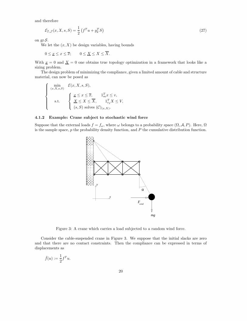
4.1.2 Example: Crane subject to stochastic wind force

Suppose that the external loads f = fω, where ω belongs to a probability space (Ω,A, P ). Here, Ωis the sample space, p the probability density function, and P the cumulative distribution function.

α

mg

Fwind

x

y

Figure 3: A crane which carries a load subjected to a random wind force.

Consider the cable-suspended crane in Figure 3. We suppose that the initial slacks are zeroand that there are no contact constraints. Then the compliance can be expressed in terms ofdisplacements as

f(u) :=1

2fT u.

20

Assume now that the crane carries a weight mg and that a wind force on the weight acts horizontallywith a random magnitude. The wind force is assumed to take values according to the probabilitydensity function shown in Figure 4. Hence the load vector f ∈ R

12 depends on the value ω = Fwind:

ω

p

ω

(ω)

=Fwind

(ω , p(ω ))i i

=P’(ω)

1 N0 iω ω ω

Figure 4: Probability density function for the wind force.

fω =

0...0ω

−mg0...0

, ω ∈ Ω = [ ω, ω ] = [ ω0, ωN ].

Since the load vector depends on ω, so does (P)(x,X), and we write (P)(x,X)(ω) for the equilibriumproblem and [u(ω), e(ω)] for its solution. Then the compliance can be written as fω(u(ω)) :=12fT

ω u(ω). This value is different for different values of the stochastic variable ω, but we need asingle value in the objective of the design optimization problem. One natural choice is to take theexpected value of the compliance as the objective. The minimum compliance problem can for thisexample then be formulated as

min(x,X,u,e)

Eω[fω(u(ω))],

s.t.

x ≤ x ≤ x, 1Tmx ≤ v,

X ≤ X ≤ X, 1Tr2

X ≤ V,

u(ω), e(ω) solves (P)(x,X)(ω), ω ∈ Ω.

The expected value is given by

Eω[fω(u(ω))] =1

2

∫ ω

ω

fTω u(ω)p(ω) dω. (28)

For each design candidate (x, X) it is in general impossible to calculate the structure’s displacementresponse u(ω) for every ω ∈ Ω, unless Ω is a discrete sample space. Hence, when Ω is continuous as

21

in this example, one way is to discretize Ω, see Figure 4. Applying Simpsons’s rule on the integralin (28), we can approximate the expected value as

Eω[fω(u(ω))] ≈ 1

2

N−1∑

i=1

fTωi

u(ωi)p(ωi)hi + hi+1

2=

1

2

∑

ℓ∈L

ρℓ(fℓ)T uℓ, (29)

where

f ℓ = fωℓ, uℓ = u(ωℓ), ρℓ = p(ωℓ)

hℓ + hℓ+1

2, L = 1, . . . , N − 1, (30)

and

hℓ = ωℓ − ωℓ−1, ℓ = 1, . . . , N. (31)

Before continuing with the problem formulation, we introduce the new notation (u, e, s, S) todenote the collection of vectors (uℓ, eℓ, sℓ, Sℓ)ℓ∈L.

Consequently, we arrive at the problem formulation

min(x,X,u,e)

1

2

∑

ℓ∈L

ρℓ(fℓ)T uℓ,

s.t.

x ≤ x ≤ x, 1Tmx ≤ v,

X ≤ X ≤ X, 1Tr2

X ≤ V,

(uℓ, eℓ) solves (P)(x,X)(ωℓ), ℓ ∈ L.

This looks like a traditional multiple load-case formulation. Here, however, the weight ρℓ (hence-forth presumed strictly positive for every ℓ ∈ L) in the objective function for each load-case isdetermined by a probability function for some event in the structure’s environment.

We can now write down the general stochastic minimum compliance problem:

(P1)

min(x,X,s,S)

cf (x, X, s, S) :=∑

ℓ∈L

ρℓEℓ(x, X, sℓ, Sℓ) =

∑

ℓ∈L

ρℓ

1

2

∑

i∈I(x)

(sℓi)

2

Exi+

∑

j∈J (X)

((LjS

ℓj)

2

2EcXj+ (g2)jS

ℓj

),

s.t.

x ≤ x ≤ x, 1Tmx ≤ v,

X ≤ X ≤ X, 1Tr2

X ≤ V,

(sℓ, Sℓ) solves (C)(x,X)(ωℓ), ℓ ∈ L.

4.1.3 Existence of optimal designs

The following result establishes the existence of optimal solutions to this problem. (We note that inthe statement of the result, the existence of a feasible solution is guaranteed whenever the boundson the design (x, X) are such that a strictly positive design is feasible, which, clearly, will alwaysbe the case.)

Theorem 4.1 (Existence of optimal solutions to (P1)). Suppose the feasible set FP1 of (P1) isnonempty. Then, there exists at least one optimal solution to (P1).

22

Proof. The design objective is to minimize a (strictly positive) weighted sum of terms with (sℓ, Sℓ)being the optimal solution to (C)(x,X)(ωℓ). Hence, by the feasibility assumption (which implies

that the functions Eℓ are proper with respect to FP1), without any loss of generality, we mayassume that all feasible solutions satisfy

Eℓ(x, X, sℓ, Sℓ) ≤ νℓ < ∞, ℓ ∈ L.

We may therefore replace the constraints of (P1) with the design constraints and the constraintsthat

(x, X, sℓ, Sℓ) ∈ grSℓ ∩ LEℓ

νℓ, ℓ ∈ L,

which forms a closed set by Corollary 3.1. Hence, the feasible set of (P1) is closed as well asnonempty. As remarked above, the upper-level objective function is proper with respect to FP1 ,and it is further lsc (cf. Lemma 3.2) and coercive, since it is coercive in (s, S) and the feasible setin terms of (x, X) is bounded. Hence, Weierstrass’ Theorem applies.

4.1.4 Convex–concave saddle-point and convex programming formulations

When the (extended) compliance is used as the upper-level design objective, the optimal designproblem can be equivalently rewritten as a convex–concave saddle-point problem, or a convex (butnondifferentiable) optimization problem. This has an immediate advantage computationally, sinceit means that the problem can be attacked by techniques from convex programming, but it can alsobe utilized as an alternative formulation when establishing, for example, the existence of optimalsolutions. In the case of the current problem (P1), the equivalent saddle-point formulation has thefollowing form:

(SP1)

find (x∗, X∗, u∗, e∗) ∈ Z × U :

J (x, X, u∗, e∗) ≤ J (x∗, X∗, u∗, e∗) ≤ J (x∗, X∗, u, e), ∀(x, X, u, e) ∈ Z × U ,

where

J (x, X, u, e) :=∑

ℓ∈L

ρℓ

1

2

m∑

i=1

xi(uℓ)T BT

i EBiuℓ +

1

2

r2∑

j=1

EcXj

L2j

(eℓj)

2 − (f ℓ)T uℓ

,

Z :=(x, X)

∣∣ (x, X) ≤ (x, X) ≤ (x, X); 1Tmx ≤ v; 1T

r2X ≤ V

,

U :=(u, e) = (uℓ, eℓ)ℓ∈L

∣∣ γTj uℓ − eℓ

j ≤ (g2)j , j = 1, . . . , r2, ℓ ∈ L

.

A convex programming formulation in terms of only displacement variables can be obtained byeliminating the design variables from the problem:

(CP1)

find (u∗, e∗) ∈ U :

J ∗(u∗, e∗) ≤ J ∗(u, e), ∀(u, e) ∈ U ,

where

J ∗(u, e) := max(x,X)∈Z

J (x, X, u, e).

23

(The function J ∗ is a finite convex function.) The minimum (extended) compliance objectiveappears if we eliminate the displacement variables: it holds that

J∗(x, X) := inf(u,e)∈U

J (x, X, u, e) = −1

2

∑

ℓ∈L

ρℓ

(fT uℓ + gT

2 Sℓ),

where Sℓ is the equilibrium tensile force solution of (C)(x,X)(ωℓ). A nested, convex optimizationformulation of the design problem in terms of the design variables only is then obtained as:

(CP2)

find (x∗, X∗) ∈ Z :

J∗(x∗, X∗) ≥ J∗(x, X), ∀(x, X) ∈ Z,

where we remark that J∗ is a concave function.Obviously, this development can be done also in the presence of unilateral contact conditions,

for the problem (P) in case the design objective is minimal extended compliance. For generalreferences on saddle-point and convex programming formulations in truss topology optimizationincluding unilateral constraints, we refer to [PeK94, PeP97].

We note, finally, that the existence of optimal solutions can be established also for more generalupper-level design objectives, as has been done, for example, in [CPW01], in the case of cable-lessstructures. Essentially, they provide two types of existence results. The first is similar to The-orem 4.1, in that it relies on Weierstrass’ Theorem, the main presumptions being the closednessof the set of feasible solutions and the coercivity of the upper-level objective function. The sec-ond result, which is close in spirit to the existence result in quadratic programming in [FrW56],amounts to replacing the coercivity assumption on the design objective with the less stringent setof assumptions that it is lower bounded on the graph of equilibrium solutions and quadratic in thelower-level variables, and further that a specially constructed lower level set is closed. The lastpresumption is equivalent to assuming that for all sufficiently good feasible designs (with respectto the design objective), the set of equilibrium displacements can be taken to lie in a compact set,a presumption which we have seen above to be a rather natural assumption to make.

4.1.5 ε-perturbation

In topology optimization, the lower design bounds (x, X) are taken to be zero. According toTheorem 4.1, this is, in principle, also legitimate from a solvability point of view. However, fordesigns with vanishing material, neither equilibrium states nor derivatives needed in a first-ordermethod may be computable. Therefore, a common strategy is to replace the zero lower designbound with a small lower bound ε > 0, thereby allowing for the computations needed in a standardnested approach.

When perturbing the problem by enforcing a lower bound ε > 0, (P)(x,X) is always uniquelysolvable, so we can switch from (C)(x,X) to (P)(x,X), as it is generally considered easier to work inthe displacement space. The ε-perturbed problem reads

(Pε1)

min(x,X,u,e)

cd(x, X, u, e) :=1

2

∑

ℓ∈L

ρℓ(fℓ)T uℓ +

1

2

∑

ℓ∈L

ρℓ

r2∑

j=1

(XjEc)

L2j

· (g2)jeℓj,

s.t.

ε1m ≤ x ≤ x, 1Tmx ≤ v,

ε1r2 ≤ X ≤ X, 1Tr2

X ≤ V,

(uℓ, eℓ) solves (P)(x,X)(ωℓ), ℓ ∈ L.

The reader should note that we use the notation cf and cd, respectively, for the design ob-jectives in the problems (P1) and (Pε

1 ), in order to distinguish the use of force and displacement

24

variables in the equilibrium conditions. However, the two objectives are equal when evaluated atequilibrium points, which is of course always the case in the structural optimization problems, andtherefore we can interchange them whenever desired. We shall also let the entire vector (u, e, s, S)[respectively, (uε, eε, sε, Sε)] be part of the optimal solution to the problem (P1) [respectively,(Pε

1)], although it is not part of the optimization formulation in its entirety. (It, however, ofcourse constitutes the solution to the primal–dual pair of problems (C)(x,X)(ωℓ) and (P)(x,X)(ωℓ)[respectively, (C)(xε,Xε)(ωℓ) and (P)(xε,Xε)(ωℓ)].)

The following result motivates the use of the above problem manipulation.

Theorem 4.2 (Convergence of ε-perturbed solutions). Suppose the feasible set FP1 of (P1) isnonempty. For each ε > 0, let (x∗

ε , X∗ε , u∗

ε, e∗ε, s

∗ε, S

∗ε ) denote an arbitrary optimal solution to

(Pε1). Then, the sequence (x∗

ε, X∗ε , s∗ε, S

∗ε ) is bounded, and converges to the optimal solution set

SOL (P1) of (P1), in the sense that

min

(x,X,s,S)∈SOL (P1)‖(x∗

ε, X∗ε , s∗ε, S

∗ε ) − (x, X, s, S)‖

→ 0.

Moreover, cf(x∗ε , X

∗ε , s∗ε, S

∗ε ) and cd(x∗

ε, X∗ε , u∗

ε, e∗ε) converges to the optimal value of (P1).

Proof. According to Theorem 4.1, an optimal solution exists to the problem (Pε1 ) for every ε > 0,

as well as to the problem (P1). Consider first the sequence (x∗ε, X

∗ε ). Clearly, this sequence is

bounded since the feasible sets of (Pε1) in (xε, Xε) are bounded, as well as that in (x, X) of (P1). We

further note that since these sets increase with a decreasing ε, the sequence cf (x∗ε , X

∗ε , s∗ε, S

∗ε )

is decreasing. In particular, it is then bounded from above. We may then use Theorem 3.1 toconclude that also the sequence (s∗ε, S∗

ε ) is bounded and further that if (x, X) is an arbitrarylimit point of the sequence (x∗

ε, X∗ε ) then (sℓ∗

ε , Sℓ∗ε ) converges to the unique optimal solution

(cf. Theorem 2.1), say, (sℓ, Sℓ), to (C)(x,X)(ωℓ), for each ℓ ∈ L.

Consider next an arbitrary feasible solution (x, X, s, S) to the problem (P1), and an arbitrarysequence (xε, Xε, sε, Sε) of feasible solutions to the problems (Pε

1 ), where however (xε, Xε) →(x, X). [For any given design (x, X) satisfying the design constraints in (P1), Proposition 1.1.2 ofAubin and Frankowska [AuF90] ensures the existence of a sequence (xε, Xε) of designs satisfyingthe design constraints in (Pε

1 ).] Corollary 3.2 then implies that the sequence (sε, Sε) of statesconverges to the limit state (s, S).

We then have that

cf (x, X, s, S) ≤ lim infε→0

cf (x∗ε , X

∗ε , s∗ε, S

∗ε )

≤ lim infε→0

cf (xε, Xε, sε, Sε)

≤ limε→0

cf (xε, Xε, s, S)

= cf (x, X, s, S), (32)

where the inequalities follow from the lsc property of cf , the optimality of (x∗ε, X

∗ε , s∗ε, S

∗ε ) and fea-

sibility of (xε, Xε, sε, Sε) in (Pε1 ), and the optimality of (sε, Sε) in (C)(xε,Xε); finally, the equality

follows from the continuity of cf (·, ·, s, S). By (32), (x, X, s, S) is optimal in (P1). The conver-gence of the sequence (x∗

ε, X∗ε , s∗ε, S

∗ε ) to the optimal solution set of (P1) then follows from its

compactness. Since cf equals cd on grSℓ, ℓ ∈ L, the last result follows also.

As remarked above, it is computationally quite often preferable to work in the displacementspace as compared to working in the force space when solving for an equilibrium. However,

25

as the lower design bound tends to zero, it seems that the sequence (u∗ε, e

∗ε) of equilibrium

displacements may be unbounded if the final design is such that the corresponding equilibriumdisplacement solution is unspecified along certain directions. This can be contrasted with theresult of Theorem 3.2 which establishes that the sequence of equilibrium displacements tends toa minimum-energy equilibrium solution for the limit design provided that the design sequencetends strictly monotonically towards it. The reason for this perhaps surprising difference is thatthe optimal designs in the ε-perturbed problems need not tend strictly monotonically to a limitdesign; certain elements of the sequence (x∗

ε , X∗ε ) may even converge finitely.

4.2 The stress-constrained minimum weight problem

4.2.1 The design optimization model

Let ρ1 > 0 be the density of the structure material and ρ2 > 0 the density of the cable material,and suppose that the effective stress is not allowed to exceed σ1 in the structure and σ2 in thecables. Since the effective stress in the structure is σe

i = |σi|, the bound in part i can be expressedas

xi|σi| ≤ σ1xi, (33)

where the factor xi has been introduced to ”remove” the constraint when there is no material tocarry any stress. Using (3) in (33), we get

|si| ≤ σ1xi.

Consider now also the effect of introducing a stochastic load in this problem. The structuralresponse depends on the stochastic variable ω. In this formulation the state variable is representedby the internal forces s and S. Previously we started with the deterministic problem and thenreplaced the state variable by its expected value. Proceeding similarly one gets:

min(x,X,s,S)

w(x, X) := ρ11Tmx + ρ21

Tr2

X,

s.t.

x ≤ x ≤ x,

X ≤ X ≤ X,

Eω[|si(ω)|] ≤ σ1xi, i = 1, . . . , m,

Eω[Sj(ω)] ≤ σ2Xj, j = 1, . . . , r2,

(s, S)(ω) solves (C)(x,X)(ω), ω ∈ Ω.

(We allow for the vectors x and X to take on infinite values.) It makes more sense to use Eω[|si(ω)|]instead of |Eω[si(ω)]| since it is more conservative. (One can get |Eω [si(ω)]| = 0 even if the stressesare very large for all events.)

Discretizing Ω into Ω = ω1, . . . , ω|L| and using Simpson’s rule as before,

Eω[|sj(ω)|] =

∫ ω

ω

|sj(ω)|p(ω) dω ≈N−1∑

i=1

|sj(ωi)|p(ωi)hi + hi+1

2=∑

ℓ∈L

ρℓ|sℓj |,

where sℓj = sj(ωℓ), and, again, ρℓ = p(ωℓ)(hℓ + hℓ+1)/2. In the same manner,

Eω[Sj(ω)] ≈∑

ℓ∈L

ρℓSℓj ,

26

and therefore we arrive at the optimization problem

min(x,X,s,S)

w(x, X) := ρ11Tmx + ρ21

Tr2

X,

s.t.

x ≤ x ≤ x,

X ≤ X ≤ X,∑

ℓ∈L

ρℓ|sℓi | ≤ σ1xi, i = 1, . . . , m,

∑

ℓ∈L

ρℓSℓj ≤ σ2Xj , j = 1, . . . , r2,

(sℓ, Sℓ) solves (C)(x,X)(ωℓ), ℓ ∈ L.

Instead of taking the expected value, we can ensure that the stresses are below the bounds for allω ∈ Ω by adding side constraints. This was not an option in the same way before, where the statevariable appeared in the objective function.3 One arrives finally at

(P2)

min(x,X,s,S)

w(x, X) := ρ11Tmx + ρ21

Tr2

X,

s.t.

x ≤ x ≤ x,

X ≤ X ≤ X,

|sℓi | ≤ σ1xi, i = 1, . . . , m, ℓ ∈ L,

Sℓj ≤ σ2Xj , j = 1, . . . , r2, ℓ ∈ L,

(sℓ, Sℓ) solves (C)(x,X)(ωℓ), ℓ ∈ L.

This is a more conservative model, and the number of side constraints is in general very large.This formulation looks like the traditional worst-case multiple load-case formulation for the stress-constrained minimum weight problem.

4.2.2 Existence of optimal designs

Theorem 4.3 (Existence of optimal solutions to (P2)). Suppose the feasible set FP2 of (P2) isnonempty. Then, there exists at least one optimal solution to (P2).

Proof. We begin by constructing a global upper bound on the energy function Eℓ(x, X, sℓ, Sℓ),ℓ ∈ L, defined in the objective of (P1), over FP2 . Consider a feasible design (x, X). Since theconstraints on (sℓ, Sℓ) are linear and Eℓ(x, X, ·, ·) is convex, the maximum, if it exists, is attainedat an extreme point (e.g., [BSS93, Theorem 3.4.7]). An upper bound of this value is obtained byconsidering only the stress constraints, as follows.

Each term in(sℓ

i)2

Exi, i ∈ I(x), when maximized with respect to sℓ

i over the set |sℓi | ≤ σ1xi,

attains its maximum at sℓi = ±σ1xi.

Each term in(LjSℓ

j)2

2EcXj+ (g2)jS

ℓj , j ∈ J (X), is either maximal at Sℓ

j = 0 or at Sℓj = σ2Xj .

Hence, we obtain that for any feasible (x, X) and ℓ ∈ L,

Eℓ(x, X, sℓ, Sℓ) ≤ 1

2

∑

i∈I(x)

xi(σ1)2E−1 +

∑

j∈J (X)

max

0,

(Xj(Ljσ2)

2

2Ec+ (g2)jσ2Xj

).

3This is true of course if we refrain from modelling our problem as a multi-objective optimization problem.The side constraints can alternatively be written as maxℓ∈L|s

ℓ

i| ≤ σ1xi, i = 1, . . . , m, whence the analogous

modification in the compliance problem leads to a min-max formulation.

27

Since the objective is to minimize the (strictly positive) weighted sum of the total weights, and

the design is nonnegative, there exists an upper bound (x, X) ≤ (x, X) on the design vector (x, X)

such that no candidate for an optimum exceeds (x, X). If we add the constraints

Eℓ(x, X, sℓ, Sℓ) ≤ 1

2

m∑

i=1

xi(σ1)2E−1 +

r2∑

j=1

maxXj≤Xj≤ bXj

0,

(Xj(Ljσ2)

2

2Ec+ (g2)jσ2Xj

)

=: νℓ < ∞, ℓ ∈ L,

we then add constraints which are redundant in the problem (P2). Moreover, according to Corol-

lary 3.1, the sets grSℓ ∩ LEℓ

νℓare closed. Hence, since the rest of the constraints are defined by

continuous functions in (x, X, sℓ, Sℓ), the feasible set of (P2) is closed, as well as nonempty. Theupper-level objective function is continuous, and coercive since the set of candidate designs (x, X)is bounded and the same is true for the set of equilibrium forces (sℓ, Sℓ), ℓ ∈ L, thanks to thestress constraints. Hence, Weierstrass’ Theorem applies.

4.2.3 ε-perturbation

In the case of a topology optimization, where (x, X) = (0, 0), for computational reasons we needto add small positive design bounds. Cheng and Guo [ChG97] have however proven that the naiveapproach—replacing the zero design bounds by ε1m ≤ x and ε1r2 ≤ X for some small positive valueof ε—will in general not generate solutions that are close to the desired ones in stress-constrainedproblems. They therefore suggested another ε-relaxation where also the stress constraints aremodified. Generalizing this procedure somewhat, and introducing the function o : R++ 7→ R++ tobe continuous and such that o(ε)/ε tends to zero while o(ε)/ε2 is bounded away from zero, asε tends to zero, we arrive at

(Pε2)

min(x,X,s,S)

w(x, X) := ρ11Tmx + ρ21

Tr2

X,

s.t.

o(ε)1m ≤ x ≤ x + o(ε)1m,

o(ε)1r2 ≤ X ≤ X + o(ε)1r2 ,

|sℓi | ≤ σ1xi + ε, i = 1, . . . , m, ℓ ∈ L,

Sℓi ≤ σ2Xi + ε, i = 1, . . . , r2, ℓ ∈ L,

(sℓ, Sℓ) solves (C)(x,X)(ωℓ), ℓ ∈ L.

Similarly to Theorem 4.2, we establish that this problem indeed gives solutions close to theones of (P2).

Theorem 4.4 (Convergence of ε-perturbed solutions). Suppose the feasible set FP2 of (P2) isnonempty. For each ε > 0, let (x∗

ε , X∗ε , s∗ε, S

∗ε ) denote an arbitrary optimal solution to (Pε

2). Then,the sequence (x∗

ε, X∗ε , s∗ε, S

∗ε ) is bounded, and converges to the optimal solution set SOL (P2) of

(P2), in the sense that

min

(x,X,s,S)∈SOL (P2)‖(x∗

ε, X∗ε , s∗ε, S

∗ε ) − (x, X, s, S)‖

→ 0.

Moreover, w(x∗ε , X

∗ε ) converges to the optimal value of (P2).

Proof. Similarly to the proof of Theorem 4.3, we will establish that the energy functionals Eℓ

are bounded on the feasible set of the problem (Pε2) for any ε > 0, by introducing an upper

28

design bound (xε, Xε) and the upper bound νℓ,ε < ∞. [In fact, it is sufficient to take (xε, Xε) =

(x + o(ε), X + o(ε)).] Using the relaxed stress constraints, the inequality (a + b)2 ≤ 2a2 + 2b2 (forany a, b ∈ R), and xi, Xi ≥ o(ε), one has

Eℓ(x, X, sℓ, Sℓ) ≤∑

i∈I(x)

(σ1xi + ε)2

2Exi+

∑

j∈J (X)

(L2

j(σ2Xj + ε)2

2EcXj+ |(g2)j |(σ2Xj + ε)

)

≤∑

i∈I(x)

(σ2

1xi

E+

ε2

Exi

)+

∑

j∈J (X)

(L2

jσ22Xj

Ec+

ε2L2j

EcXj+ |(g2)j |(σ2Xj + ε)

)

≤m∑

i=1

(σ2

1(xε)i

E+

1

Eo(ε)/ε2

)

+

r2∑

j=1

(L2

jσ22(Xε)j

Ec+

L2j

Eco(ε)/ε2+ |(g2)j |(σ2(Xε)j + ε)

)

=: νℓ,ε < ∞, ℓ ∈ L,

where νℓ,ε are bounded as ε → 0 since o(ε)/ε2 stays bounded away from zero. We conclude

that the sequence (x∗ε, X

∗ε , s∗ε, S

∗ε ) is bounded. Suppose that (x∗, X∗, s∗, S∗) is a limit point of

this sequence. Invoking Theorems 2.2 and 3.1 then yields that (s∗, S∗) is the optimal solution to(C)(x∗,X∗)(ωℓ), ℓ ∈ L. The continuity properties of the other constraints of the problem (P2) then

imply that (x∗, X∗, s∗, S∗) is feasible in (P2). Let (x, X, s, S) be an arbitrary feasible solution to(P2), set xε = x + o(ε)1m, Xε = X + o(ε)1r2 and let (sℓ

ε, Sℓε) solve (C)(xε,Xε)(ωℓ), ℓ ∈ L.

We then have, by Theorem 3.3, that for some κ > 0 and every i = 1, . . . , m and ℓ ∈ L,

|(sℓε)i|≤κo(ε) + |sℓ

i |≤κo(ε) + σ1[xi − o(ε) + o(ε)]=(κ − σ1)o(ε) + σ1(xε)i≤σ1(xε)i + ε,

for all ε small enough, where we have used the assumption that o(ε)/ε → 0. Sε can be treated inthe same way, and since clearly (xε, Xε) satisfies the design constraints, (xε, Xε, sε, Sε) is permis-sible in (Pε

2 ). Hence, w(x∗ε , X∗

ε ) ≤ w(xε, Xε). Letting ε tend to zero in this inequality, we obtainthat w(x∗, X∗) ≤ w(x, X), whence we may conclude that (x∗, X∗, s∗, S∗) solves (P2). The resultthen follows from the compactness of SOL (P2) and the continuity of w.

4.2.4 Example: One-bar truss with a cable revisited

Consider again the one-dimensional structure in Figure 1. Assume that allowable stresses areσ1 = 1 and σ2 = 1/2 for the bar and cable material, respectively. Invoking the stress constraints|s| ≤ x and S ≤ X/2, the nested version of (P2) with x = X = 0 becomes

min(x,X)

x + X,

s.t.

x ≥ 0, X ≥ 0, x + X > 0,

x ≤ (x + X)x,

X ≤ (x + X)X/2,

recalling (19). We presume the upper design bounds are passive. The admissible domain is shownin Figure 2.

One sees immediately from the figure that the optimal solution is

x∗ = 1, X∗ = 0, with optimal weight = x∗ + X∗ = 1.

29

When this type of optimal solution and design domain appears, in the structural optimization com-munity one talks about the ”stress singularity phenomenon”, and the optimal solution is sometimesreferred to as a ”singular topology”. The first example of a singular topology was reported by Svedand Ginos [SvG68], and design domains very similar to the one in Figure 2 were presented by Kirsch[Kir90] and later also by Rozvany and Birker [RoB94] and by Cheng [Che95].

From a mathematical programming point of view, the singularity stems from the constraintsnot being qualified (in the sense of, for example, Slater), cf. [BSS93, DuB98]. This implies that theKarush–Kuhn–Tucker (KKT) conditions need not be necessary for (local) optimality. [Obviously,the nonconvexity of the problem adds to this the fact that the KKT conditions neither are sufficientfor (local) optimality.] Almost every practical numerical algorithm generates solutions that are onlyguaranteed to fulfill the KKT conditions [e.g., (x, X) = (2, 0) in Figure 2], which, hence, need nothave anything to do with the desired global (or even local) minima. If small strictly positive lowerdesign bounds are enforced, that is, x = X = ε, then one gets the incorrect ”optimal” weight 2,and the optimal solutions (x∗

ε , X∗ε ) satisfy

‖(x∗, X∗) − (x∗ε , X

∗ε )‖ ≥ 1√

2, ∀ε ∈ (0, 1),

so the straightforward ε-perturbation is clearly incorrect.In this example, the stress bounds were chosen differently in the bar and cable. When the elastic

modulii, specific weights and stress bounds are uniform, then, for a single load, the problem (P2)seems to provide no major complications; in fact optimal solutions can, at least in the non-unilateralcase, be obtained by solving a dual pair of linear programs [DGG64, Sva94]. However, since it isvery plausible that one wishes to use cable and bar materials that are not the same, or that they aresubject to different allowable stresses, one must deal with this type of problem. Moreover, Stolpeand Svanberg [StS01] showed that multiple loads (while keeping the other data uniform) suffice toproduce difficult problem instances, where global optima are situated at degenerate parts of thefeasible domain. Since multiple load-cases appear after discretization of the probability space, thismeans that one can expect the optimal solution to be singular, even if the elastic modulii, specificweights and stress bounds are uniform.

Let us now consider the example in view of the ε-relaxed (or, ε-perturbed) statement (Pε2). We

take o(ε) := ε2, so x = X = ε2, presume the upper bounds to be passive, and write the stressconstraints on the form

|s| ≤ x + ε, S ≤ X/2 + ε.

Then the nested version of (Pε2 ) becomes

min(x,X)

x + X,

s.t.

x ≥ ε2, X ≥ ε2,

x ≤ (x + X)(x + ε),

X ≤ (x + X)(X/2 + ε).

The admissible domain for ε = 0.1 is shown in Figure 5.The optimal solution, for a general ε > 0, is given by

x∗ε =

1 − 5ε +√

1 − 2ε + 9ε2

2, X∗

ε =x∗

ε

x∗ε + ε

− x∗ε ,

and the optimal weight is x∗ε/(x∗

ε + ε). Clearly,

limε→0

x∗ε = x∗, lim

ε→0X∗

ε = X∗,

as Theorem 4.4 predicts.

30

x

constant weight

0.5 1 1.5

0.5

1

1.5

X

Figure 5: The admissible design domain for ε = 0.1. The optimal solution is at the black circle.

5 FE-discretized sheets in contact

5.1 The design optimization model

Consider a family of linearly elastic continua occupying a region B(h) in space,

B(h) = (ξ1, ξ2, ξ3) ∈ R3 | (ξ1, ξ2) ∈ Ω, |ξ3| < h(ξ1, ξ2)/2 ,

where Ω is a fixed open and plane two-dimensional set and h : Ω → R+ is a thickness function.Note that the topology of B(h) can be changed by introducing holes through setting h(ξ1, ξ2) = 0.

We assume that B(h) is loaded in such a way that the state of stress is plane. The designobjective now is to minimize the (in some sense) effective stress σM : B(h) → R+. It would havebeen desirable to minimize the maximum effective stress, that is, ‖σM‖L∞(B(h)), but since σM isonly guaranteed to belong to L2, we instead choose

‖σM‖2L2(B(h)) =

∫

B(h)

σ2M dB

=

∫

Ω

∫ h(ξ1,ξ2)/2

−h(ξ1,ξ2)/2

σ2M dξ3dξ1dξ2

=

∫

Ω

hσ2M dξ1dξ2 (plane stress)

≈m∑

i=1

hiAi(σei )

2 (FE-discretization step)

=∑

i∈I(x)

xiσTi Mσi, (xi is the material volume) (34)

where Ai is the area of the finite element, σTi = (σx, σy, τxy), and M is a positive definite and

symmetric matrix, cf. Section 2.1. Finally, using (3), we get

‖σM‖2L2(B(h)) ≈

∑

i∈I(x)

sTi Msi

xi. (35)

31

We assume that the unilateral constraints are due to rigid supports, so no cables are present, thatis, the variables (S, e) do not appear in the equilibrium problems and x is the only design variable.The energy function hence now takes the form

E(x, s, λ) =1

2

∑

i∈I(x)

sTi E−1si

xi+ gT

1 λ

whenever it is finite. If the initial gaps are zero, that is, if g1 = 0, then compliance is equal to12

∑i∈I(x)

sTi E−1si

xi, which is obtained in (35) by choosing M = 1

2E−1. By choosing the matrix

given in Section 2.1 one minimizes the L2-norm of the von Mises effective stress. We enforce anupper bound on the available material volume,

∫B(h) dB ≤ v. Further,

∫

B(h)

dB =

∫

Ω

∫ h(ξ1,ξ2)/2

−h(ξ1,ξ2)/2

dξ3dξ1dξ2

=

∫

Ω

h dξ1dξ2

≈m∑

i=1

hiAi (FE-discretization step)

=

m∑

i=1

xi, (36)

so the constraint becomes 1Tmx ≤ v. Including stochastic loads and performing a discretization of

the probability space as before, we can pose the following problem statement:

(P3)

min(x,s,λ)

cf,M (x, s) :=∑

ℓ∈L

ρℓ

∑

i∈I(x)

(sℓi)

T Msℓi

xi,

s.t.

1T

mx ≤ v, x ≥ 0,

(sℓ, λℓ) solves (C)(x)(ωℓ), ℓ ∈ L.

For more details on how to arrive at the mathematical programming problem by FE-discretization,we refer to [PeH98].

5.2 Existence of optimal designs

The following result is proven similarly to Theorem 4.1.

Theorem 5.1 (Existence of optimal solutions to (P3)). Suppose the feasible set FP3 of (P3) isnonempty. Then, there exists at least one optimal solution to (P3).

Proof. Since cf,M is to be minimized, we can presume that FP3 is such that cf,M is proper withrespect to FP3 , and even bounded from above on FP3 (or construct it as such, by introducing anadditional redundant constraint of the form cf,M (x, s) ≤ ν, with ν < ∞). Matrix norms beingessentially equivalent, we obtain, for some κ > 0, that

∑

ℓ∈L

ρℓEℓ(x, sℓ, λℓ) ≤ κcf,M (x, s) +∑

ℓ∈L

ρℓgT1 λℓ

= κcf,M (x, s) +∑

ℓ∈L

ρℓgT1 C1[f

ℓ − BT sℓ] (37)

32

holds for all (x, s, λ) ∈ FP3 , where the equality stems from the quasi-orthogonality of C1 and theequilibrium conditions. This implies that without any loss of generality we may add constraints ofthe form

Eℓ(x, sℓ, λℓ) ≤ νℓ + (aℓ)T sℓ, ℓ ∈ L, (38)

to the constraints of the problem (P3), for some appropriate choice of (aℓ, νℓ). By the lsc propertyof the energy functional, the corresponding set is closed. Due to the relation (37), and Corol-lary 3.1, the intersection of these new constraints with the graphs grSℓ, ℓ ∈ L, is nonempty andclosed. Hence, the feasible set of (P3) is nonempty and closed. The upper-level objective functionis (again by assumption) proper, and it is further lsc and coercive, since it is coercive in s (Mbeing positive definite, cf. further Lemma 3.2 and the proof of Theorem 2.1) and the feasible setin terms of x is bounded. Hence, Weierstrass’ Theorem applies.

5.3 ε-perturbation

When perturbing the problem by enforcing a volume lower bound ε > 0, (P)(x) is always uniquelysolvable, so we can switch from (C)(x) to (P)(x). Then we have to note that, by using (4), thedesign objective becomes

‖σM‖2L2(B(h)) ≈

m∑

i=1

xiuT BT

i EMEBiu.

Therefore, by setting Mi = BTi EMEBi, we can pose

(Pε3)

min(x,u)

cd,M (x, u) :=∑

ℓ∈L

ρℓ

m∑

i=1

xi(uℓ)T Miu

ℓ,

s.t.

1T

mx ≤ v + εm, x ≥ ε1m,

uℓ solves (P)(x)(ωℓ), ℓ ∈ L.

Similarly to Theorem 4.2, we establish that this problem indeed gives optimal solutions closeto the ones of (P3).

Theorem 5.2 (Convergence of ε-perturbed solutions). Suppose the feasible set FP3 of (P3) isnonempty. For each ε > 0, let (x∗

ε , u∗ε, s

∗ε, λ

∗ε) denote an arbitrary optimal solution to (Pε

3 ). Then,the sequence (x∗

ε , s∗ε, λ

∗ε) is bounded, and converges to the optimal solution set SOL (P3) of (P3),

in the sense that

min(x,s,λ)∈SOL (P3)

‖(x∗ε , s

∗ε, λ

∗ε) − (x, s, λ)‖

→ 0.

Moreover, cf,M (x∗ε , s

∗ε) and cd,M(x∗

ε , u∗ε) converge to the optimal value of (P3).

Proof. According to Theorem 5.1, an optimal solution exists to the problem (Pε3) for every ε > 0

(since also cd,M is coercive whenever ε > 0), as well as to the problem (P3). Consider first thesequence x∗

ε. Clearly, this sequence is bounded since the feasible sets of (Pε3) in xε are bounded,

as well as that in x of (P3). The sequence cf,M (x∗ε , s

∗ε) is bounded as well. To see this, consider,

for any ε > 0, an optimal solution, say (x∗ε , s

∗ε), to the problem which equals (Pε

3) except that the

33

volume constraint is [the original from (P3)] 1Tmx ≤ v. (This problem clearly has optimal solutions

for every ε > 0 small enough.) Then, obviously,

0 ≤ cf,M (x∗ε, s

∗ε) ≤ cf,M (x∗

ε , s∗ε)

holds, and the sequence cf,M (x∗ε , s

∗ε) is furthermore monotonically decreasing (hence upper

bounded), since the feasible set of the corresponding problem increases monotonically with a de-creasing value of ε.

Since cf,M (x∗ε , s

∗ε) is bounded, so is the sequence (s∗ε, λ∗

ε). Further, by (37) and Theo-rem 3.1, if x is an arbitrary limit point of the sequence x∗

ε then (s∗ε, λ∗ε) converges to the

optimal solution (cf. Theorem 2.1), say, (s, λ), to the problems (C)(x)(ωℓ), ℓ ∈ L.

Consider next an arbitrary feasible solution (x, s, λ) to the problem (P3), let xε := x + ε1m,(sε, λε) be the optimal solution to the problems (C)(xε)(ωℓ), ℓ ∈ L, and uε the optimal solutions to

the problems (P)(xε)(ωℓ), ℓ ∈ L. Clearly, (xε, sε, λε) is a feasible solution to (Pε3). Corollary 3.2

implies that the sequence (sε, λε) of states converges to the limit state (s, λ). Further, Theo-rem 3.2 states that the sequence uε converges to the least-energy displacement solution, heredenoted u, to the problems (P)(x)(ωℓ), ℓ ∈ L.

We then have that

cf,M (x, s) ≤ lim infε→0

cf,M (x∗ε , s

∗ε)

≤ lim infε→0

cf,M (xε, sε)

= limε→0

cd,M (xε, uε)

= cd,M (x, u)

= cf,M (x, s), (39)

where the inequalities follow from the lsc property of cf,M and the optimality of (x∗ε , s

∗ε, λ

∗ε) and

feasibility of (xε, sε, λε) in the problem (Pε3), and the equalities follow from the identity between

cf,M and cd,M on the equilibrium sets grSℓ, ℓ ∈ L, the continuity of cd,M , and again from theidentity between cf,M and cd,M on the equilibrium set. By (39), (x, s) is optimal in (P3). Theconvergence of the sequence (x∗

ε, s∗ε, λ

∗ε) to the optimal solution set of (P3) then follows from its

compactness. Since cf,M equals cd,M on grSℓ, ℓ ∈ L, the last result follows also.

With the available proof techniques, an ε-perturbation of the volume constraint was neededin the definition of (Pε

3), even though we suspect Theorem 5.2 may be true also without it. Forinstance, it can be shown that the ε-relaxation is not necessary with respect to the total volumeconstraint in the problem (Pε

3) if M = E−1, since, in this case, the design objective equals that ofthe problems (C)(x)(ωℓ), ℓ ∈ L, whence we obtain that

cf (x, s) ≤ lim infε→0

cf (x∗ε , s

∗ε)

≤ lim infε→0

cf (xε, sε)

≤ limε→0

cf (xε, s)

= cf (x, s),

where the equality follows from the continuity of cf (·, s) [cf. Lemma 3.1].We finally note that in order to avoid checkerboard-like numerical instabilities, it may be

necessary to slightly change the design parametrization by assigning the same thickness value tomore than one finite element. For instance, triangular elements could be ordered in neighboringpairs and assigned the same thickness.

34

6 Concluding remarks and further research

In this paper, we have considered quite general problems in structural topology optimization ofunilaterally constrained mechanical structures. This class of optimization problems provides sev-eral difficulties, such as principal problems connected to the alteration of topology; for instance,many permissible designs lack equilibria. The remedy to this problem, achieved by providing andvalidating ε-perturbations that transform the problem statement to a sizing form, is one of themain themes of this paper. However, even if the topology has been fixed in the sizing problem, thedesign–to–state mappings are only locally Lipschitz continuous and generally not differentiable.This is due to the inclusion of unilateral constraints in the equilibrium formulations. Therefore,when including mechanical contact or cables, the nested versions of the structural optimizationproblems are not differentiable.

In the future we will investigate appropriate numerical solution algorithms for some of theproblems investigated—a topic which is not covered in this paper. The monograph [LPR96] in-cludes several algorithms for this class of problems, such as the implicit programming algorithmfor the nested problem, and the penalty interior point algorithm for the simultaneous version ofthe problem, cf. also [OKZ98, HKP99a]. The nested problem can in principle be treated by anymethod from nondifferentiable optimization, for example, bundle methods ([OKZ98]) and subgra-dient methods ([CPW01]). Another possibility is to use smoothing (cf. [FJQ99, Hil00]), that is,to replace the equilibrium problem by a sequence of smooth approximations. Then any standardfirst-order algorithm, such as sequential explicit approximation methods, can be used for the nestedproblem.

As always in structural optimization, nonconvexity is a potential problem, in that first-ordermethods may terminate at non-global, local optima, corresponding to rather inefficient structures.Sometimes this seems to be especially pronounced in ε-relaxed topology optimization (cf. [StS01])and in optimization in unilateral mechanics. In [Hil00], it was however reported that a smoothingmodification may improve a first-order algorithm’s ability to avoid (non-global) local optima thatare due to the presence of unilateral constraints.

Compliance minimization is a rare special instance of the class of structural optimization prob-lems, since it can be formulated as convex optimization problems and convex–concave saddle-pointproblems. Moreover, in the nested approach, the derivatives (when they exist) of compliancewith respect to changes in designs, are very cheap to calculate. For other structural optimizationproblems, such as stress-constrained problems, the constraints are numerous, and the sensitivityanalyses can be expected to require much more computational time.

In this paper, we handled stochastic forces through a straightforward discretization of thesample space. Other data can also be allowed to be random, such as the gaps g1 or initial cableslacks g2, as a way of accounting for mounting uncertainties. Moreover, alternative probabilityspace discretizations, or other means to handle stochastic data, are possible and will be investigated,as well as the most natural choices of objective functions in the more general settings mentioned.

The aggregate effects on the proper choices of numerical procedures, of all the generalizationsof design problems previously considered which we have either investigated in detail in this paperor only briefly mentioned, will be the subject of substantial forthcoming theoretical and numericalinvestigations. Some of the complications introduced because of the added complexity have alreadybeen mentioned in this section; some others, pertaining to the introduction of stochastic data, arediscussed in [CPW01].

Acknowledgments

The authors would like to thank the anonymous referees for several valuable remarks.

35

References

[Ach98] W. Achtziger, Multiple-load truss topology and sizing optimization: Some properties ofminimax compliance, Journal of Optimization Theory and Applications, 98 (1998), pp. 255–280.

[AuF90] J.-P. Aubin and H. Frankowska, Set-Valued Analysis, Birkhauser, Boston, 1990.

[BGK+83] B. Bank, J. Guddat, D. Klatte, B. Kummer, and K. Tammer, Nonlinear parametric

optimization, Birkhauser Verlag, Basel, 1983.

[BSS93] M.S. Bazaraa, H.D. Sherali, and C.M. Shetty, Nonlinear Programming: Theory and

Algorithms, John Wiley & Sons, New York, NY, 2nd edition, 1993.

[Bro66] F.E. Browder, Existence and approximation of solutions of nonlinear variational inequalities,Proceedings of the National Academy of Sciences, U.S.A., 56 (1966), pp. 1080–1086.

[Che95] G.D. Cheng, Some aspects of truss topology optimization, Structural Optimization, 10 (1995),pp. 173–179.

[ChG97] G.D. Cheng and X. Guo, ε-relaxed approach in structural topology optimization, Structural

Optimization, 13 (1997), pp. 258–266.

[CPW01] S. Christiansen, M. Patriksson, and L. Wynter, Stochastic bilevel programming in struc-tural optimization, Structural and Multidisciplinary Optimization, 21 (2001), pp. 361–371.

[DGG64] W.S. Dorn, R.E. Gomory, and H.J. Greenberg, Automatic design of optimal structures,Journal de Mecanique, 3 (1964), pp. 25–52.

[DuB98] P. Duysinx and M.P. Bendsøe, Topology optimization of continuum structures with localstress constraints, International Journal for Numerical Methods in Engineering, 43 (1998),pp. 1453–1478.

[FJQ99] F. Facchinei, H. Jiang, and L. Qi, A smoothing method for mathematical programs withequilibrium constraints. Mathematical Programming, 85 (1999), pp. 107–134.

[FrW56] M. Frank and P. Wolfe, An algorithm for quadratic programming, Naval Research Logistics

Quarterly, 3 (1956), pp. 95–110.

[Hil00] D. Hilding, A heuristic smoothing procedure for avoiding local optima in optimization ofstructures subject to unilateral constraints, Structural and Multidisciplinary Optimization, 20(2000), pp. 29–36.

[HKP99a] D. Hilding, A. Klarbring, and J.-S. Pang, Minimization of maximum unilateral force,Computer Methods in Applied Mechanics and Engineering, 177 (1999), pp. 215–234.

[HKP99b] D. Hilding, A. Klarbring, and J. Petersson, Optimization of structures in unilateralcontact, Applied Mechanics Reviews, 52 (1999), pp. 139–160.

[Kir90] U. Kirsch, On singular topologies in optimum structural design, Structural Optimization, 2(1990), pp. 133–142.

[LPR96] Z.-Q. Luo, J.-S. Pang, and D. Ralph, Mathematical Programs with Equilibrium Con-

straints, Cambridge University Press, Cambridge, UK, 1996.

[LuT92] Z.-Q. Luo and P. Tseng, Error bound and convergence analysis of matrix splitting algorithmsfor the affine variational inequality problem, SIAM Journal on Optimization, 2 (1992), pp. 43–54.

[LuT97] Z.-Q. Luo and P. Tseng, On a global projection-type error bound for the linear complemen-tarity problem, Linear Algebra and Its Applications, 253 (1997), pp. 251–278.

[OKZ98] J. Outrata, M. Kocvara, and J. Zowe, Nonsmooth Approach to Optimization Problems

with Equilibrium Constraints, Kluwer Academic Publishers, Dordrecht, 1998.

[PeH98] J. Petersson and J. Haslinger, An approximation theory for optimum sheets in unilateralcontact, Quarterly of Applied Mathematics, 56 (2) (1998), pp. 309–325.

36

[PeK94] J. Petersson and A. Klarbring, Saddle point to stiffness optimization of discrete structuresincluding unilateral contact, Control and Cybernetics, 3 (1994), pp. 461–480.

[PeP97] J. Petersson and M. Patriksson, Topology optimization of sheets in contact by a subgradi-ent method, International Journal of Numerical Methods in Engineering, 40 (1997), pp. 1295–1321.

[Rob80] S.M. Robinson, Strongly regular generalized equations, Mathematics of Operations Research,5 (1980), pp. 43–62.

[Rob91] S.M. Robinson, An implicit-function theorem for a class of nonsmooth functions. Mathematics

of Operations Research, 16 (1991), pp. 282-309.

[Roc70] R.T. Rockafellar, Convex Analysis, Princeton University Press, Princeton, NJ, 1970.

[Roz01] G.I.N. Rozvany, On design-dependent constraints and singular topologies, Structural and

Multidisciplinary Optimization, 21 (2001), pp. 164–172.

[RoB94] G.I.N. Rozvany and T. Birker, On singular topologies in exact layout optimization, Struc-

tural Optimization, 8 (1994), pp. 228–235.

[Sta69] G. Stampacchia, Variational Inequalities, Pubblicazioni IAC, Serie III - N. 25, Rome, 1969.

[StS01] M. Stolpe and K. Svanberg, On the trajectories of the ε-relaxation approach for stress-constrained truss topology optimization, Structural and Multidisciplinary Optimization, 21(2001), pp. 140–151.

[Sva94] K. Svanberg, Global convergence of the stress ratio method for truss sizing, Structural Opti-

mization, 8 (1994), pp. 60–68.

[SvG68] G. Sved and Z. Ginos, Structural optimization under multiple loading, International Journal

of Mechanical Sciences, 10 (1968), pp. 803–805.

37