network-based modeling of coupled electro-mechanical systems€¦ · network-based modeling of...

Network-based Modeling ofCoupled Electro-Mechanical

Systems

L. ScholzTechnische Universität Berlin

ERC GrantModeling, Simulation and Controlof Multi-Physics Systems

MATHMOD 2012, Vienna, February 15th, 2012

Outline

1 Introduction2 Modeling of coupled electro-mechanical systems3 Remodeling and index analysis

Minimal extension for mechanical subsystemsMinimal extension for electrical subsystemsThe Index of the Coupled System

4 Numerical Example

L. Scholz (TU Berlin) Network-based Modeling of Coupled Systems MATHMOD 2012, 15.02.2012 2 / 24

Modeling of multi-physical Systems

. Modularized network-based modeling of multi-physics systems leads todifferential-algebraic equations (DAEs).

. In most simulation environments algebraic constraints are resolved toobtain a system in state space form.I application to large-scale systems not possible (or expensive)I complicated formulas with doubtful numerical propertiesI numerical solution deviates from constraints/interface conditions (e.g.

numerical damping or numerical dissipation).Regularization/remodeling techniques for large-scale high-index DAEs!L. Scholz (TU Berlin) Network-based Modeling of Coupled Systems MATHMOD 2012, 15.02.2012 3 / 24

Outline



4 Numerical Example


Mechanical subsystems

p = vM(p)v = f (t, p, v , u)− GT (p, u)λ

0 = g(p, u)(EoM)

. positions p ∈ Rnp , velocities v ∈ Rnp , holonomic constraintsg(p, u) ∈ Rnc , inputs u ∈ Rnu , f (t, p, v , u) applied forces, GT (p, u)λconstraint forces.

. The mass matrix M(p) is positive definite and the constraint matrixG (p, u) := ∂g(p,u)

∂p has full row rank.

Properties:. d-index 3 DAE. hidden constraints on velocity level: d

dt g(p, u) = 0

. hidden constraints on acceleration level: d2

dt2g(p, u) = 0. consistent initial values for p(t0), v(t0), λ(t0) are requiredL. Scholz (TU Berlin) Network-based Modeling of Coupled Systems MATHMOD 2012, 15.02.2012 5 / 24

Electrical Subsystems

ACddt qC (AT

C η, u, t) + AR r(ATR η, u, t) + ALıL + AV ıV + AI I s(u, t) = 0

ddtφL(ıL , u, t)− AT

L η = 0

ATV η −V s(u, t) = 0

. for lumped electrical circuit modeled via the Modified Nodal Analysis

. incidence matrix A = [AC AL AR AV AI ], node potentials η,branch voltages νT =

[νTC νTL νTR νTV νTI

], branch currents

ıT =[ıTC ıTL ıTR ıTV ıTI

].

. I s ,V s describe currents of current sources and voltages of voltagesources; r describes the resistance, qC describes the charges ofcapacitances, φL describes the fluxes of inductances.


The index of the MNA equations

Theorem (Estévez Schwarz & Tischendorf 2000)Assume that no loops of voltage sources/cutsets of current sources exists,all circuit elements are passive and controlled sources are not part ofCV-loops or LI-cutsets.1. If the circuit contains no voltage sources and every node is connected

with every other node via a capacitive path the DAE has d-index 0.2. If there are neither LI-cutsets nor CV-loops the DAE has d-index 1.

3. If there exist LI-cutsets or CV-loops the DAE has d-index 2.

. hidden constraints (in case of CV-loops or LI-cutsets)

0 = QTC R V

(AL

ddt ıL + AI

ddt I s(∗)

)0 = QT

V−C

(AT

V ,indddt η − d

dtV ind(t))

. The projectors QV−C and QCVR can be determined purely based ongraph theoretical algorithms.


Coupled Electro-Mechanical Systems

. Each subsystem Si with states xi ∈ Rni , inputs ui ∈ Rpi is given by

Fi(t, xi , xi , ui , ui) = 0

. coupling of subsystem Si with Sj1 , . . . ,Sjk via the condition

ui = Gi ,j1,...,jk (t, xj1 , . . . , xjk ),

. Fi and Gi ,j1,...,jk are assumed to be sufficiently smooth.

. We restrict to coupled systems consisting only of S1 and S2, andthe coupling is done via ui = Gi ,j(t, xj), i , j = 1, 2, i 6= j .

S1

S2

y1

u2

u1

y2


Outline



4 Numerical Example


Remodeling of Coupled System

Coupling of subsystems can easily lead to large-scale high-index DAEs. numerical instabilities can occur. drift of numerical solution from constraint manifold. inaccuracies/order reduction of numerical methods, oscillations

Two-step remodeling procedure1. Each subcomponent is remodeled using index reduction by

minimal extensionI the special structure of the subsystem is incorporatedI in the resulting index 1 system all explicit and implicit constraints are

available (→ initialization easy, no drift of numerical solution)I the variables keep their physical meaning

2. The index of the coupled system constructed by coupling theequivalent index-1 formulations is analyzed.


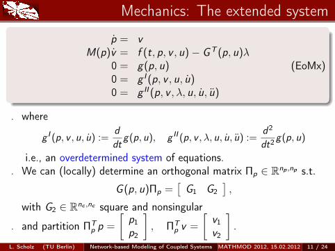
Mechanics: The extended system

p = vM(p)v = f (t, p, v , u)− GT (p, u)λ

0 = g(p, u)0 = g I (p, v , u, u)0 = g II (p, v , λ, u, u, u)

(EoMx)

. where

g I (p, v , u, u) :=ddt

g(p, u), g II (p, v , λ, u, u, u) :=d2

dt2g(p, u)

i.e., an overdetermined system of equations.. We can (locally) determine an orthogonal matrix Πp ∈ Rnp ,np s.t.

G (p, u)Πp =[G1 G2

],

with G2 ∈ Rnc ,nc square and nonsingular

. and partition ΠTp p =

[p1p2

], ΠT

p v =

[v1v2

].


Mechanics: Index-1 Formulation

Introducing new variables w1 for p2 and w2 for v2 gives

p1 = v1w1 = v2

M(p)Πp

[v1w2

]= f (t, p, v , u)− GT (p, u)λ

0 = g(p, u)0 = g I (p, v , u, u)0 = g II (p, v , λ, u, u, u)

(EoM1)

Properties:. d-index 1. no hidden constraints. no drift of the solution manifold. equivalent formulation, i.e. same solution for (p, v , λ).L. Scholz (TU Berlin) Network-based Modeling of Coupled Systems MATHMOD 2012, 15.02.2012 12 / 24

Electrics: The extended system

0 = ACddtqC (AT

C η, t) + AR g(ATR η, t) + ALıL + AV ıV + AI I s(∗)

0 = ddtφL(ıL , t)− AT

L η

0 = ATV η −V s(∗)

0 = QTV−CA

TV ,ind

ddt η − QT

V−CddtV ind(t)

0 = QTC R VAL

ddt ıL + QT

C R VAIddt I s(∗)

For hidden constraints due to CV-loops:. Find transformation Πη (permutation!) such that

QTV−CA

TV ,indΠ−1

η = [F1 F2], F1 nonsingular.

. Partition and introducing the new variable

η = Πηη =

[η1η2

], η1 =

ddtη1


Electrics: The extended system

0 = AC C (.)ATC

ddt η + ACqC ,t + AR g(AT

R η, t) + ALıL + AV ıV + AI I s(∗)0 = L(.) d

dt ıL + φL,t − ATL η

0 = ATV η −V s(∗)

0 = QTV−CA

TV ,ind

ddt η − QT

V−CddtV ind(t)

0 = QTC R VAL

ddt ıL + QT

C R VAIddt I s(∗)

using C (.) := ∂qC∂νC

, qC,t(.) := ∂qC∂t , L(.) := ∂φL

∂ıL, φL,t(.) := ∂φL

∂t .

For hidden constraints due to CV-loops:. Find transformation Πη (permutation!) such that

QTV−CA

TV ,indΠ−1

η = [F1 F2], F1 nonsingular.

. Partition and introducing the new variable

η = Πηη =

[η1η2

], η1 =

ddtη1


Electrics: The extended system (2)

0 = AC C (.)ATC

[η1ddt η2

]+ ACqC,t(.) + AR g(.) + ALıL + AV ıV + AI I s(∗)

0 = L(ıL , t) ddt ıL + φL,t(ıL , t)− AT

L η

0 = ATV η −V s(∗)

0 = QTC R V AL

ddt ıL + QT

C R V AIddt I s(∗)

0 = F1η1 + F2 ddt η2 − QT

V−CddtV ind (t)

(with A∗ := ΠηA∗). Order the nodes and branches such that

QTC R VAL =

[AL 0 I

], QT

C R VAI =[AI ,ind 0

]. Using this splitting we can rewrite the hidden constraints as

0 = ALddtıL +

ddtıL + AI ,ind

ddt

I ind(t).


Electrics: Index-1 formulation

0 = AC C (.)ATC

[η1ddt η2

]+ ACqC,t(.) + AR g(.) + ALıL + AV ıV + AI I s(∗)

0 = L(.)

ddt ıLddt ıL

−ALddt ıL − AI ,ind

ddt I ind (t)

+ φL,t(.)− ATL η

0 = ATV η −V s(∗)

0 = F2 ddt η2 + F1η1 − QT

V−CddtV ind (t)

Properties:. d-index 1. no hidden constraints. no drift from the solution manifold. equivalent to MNA equations (i.e. same solution for η, ıL , ıV )


Index analysis for the coupled system. Consider the equivalent index-1 formulation of subsystem Si :

xi ,1 = k i1(t, xi ,1, xi ,2, ui )0 = k i2(t, xi ,1, xi ,2, ui , ui )

with∂k i2∂xi ,2

nonsingular,

. and the coupled system

X1 = K1(t,X1,X2),

0 = K2(t,X1,X2, X1, X2),(1)

with X1 =

[x1,1x2,1

], X2 =

[x1,2x2,2

]and

K1(.) =

[k11 (t, x1,1, x1,2,G1,2(t, x2,1, x2,2))k21 (t, x2,1, x2,2,G2,1(t, x1,1, x1,2))

],

K2(.) =

[k12 (t, x1,1, x1,2,G1,2(t, x2,1, x2,2), d

dtG1,2(t, x2,1, x2,2))

k22 (t, x2,1, x2,2,G2,1(t, x1,1, x1,2), ddtG2,1(t, x1,1, x1,2))

].


Index-1 condition

Theorem

. Then, the coupled system (1) is of d-index 0 (i.e. an ODE), iff

K2;X2=

[k12;x12

k12;x22

k22;x12k22;x22

]is nonsingular.

. If[K2;X1

K2;X2

]≡ 0, then the coupled system is of d-index 1, iff

K2;X2 =

[k12;x12

k12;x22

k22;x12k22;x22

]is nonsingular. (2)

. If no derivatives of inputs occur (2) is always fulfilled (coupling only viadifferential variables or no loops over algebraic variables)

. In general an increase of the index will occur if the input function isdifferentiated.


Outline



4 Numerical Example


Numerical Example - The Dynamo



x = vy = w

mv = − sin(α)λ− cos(α)Fw (ϕ, ı)mw = −mg − cos(α)λ+ sin(α)Fw (ϕ, ı)

0 = sin(α)x + cos(α)y

C η = −Gη − ı0 = η − Vs(t, ϕ, ϕ)

ϕ(v)ı

d-index 3

d-index 2

The coupled system has d-index 4!

Fz Fg

Fw

F

α

h l

b

m

+

+

−−

+

GC

Vs



x = vy = w

mv = − sin(α)λ− cos(α)Fw (ϕ, ı)mw = −mg − cos(α)λ+ sin(α)Fw (ϕ, ı)

0 = sin(α)x + cos(α)y

C η = −Gη − ı0 = η − Vs(t, ϕ, ϕ)

ϕ(x)ı

d-index 3

d-index 2


Fz Fg

Fw

F

α

h l

b

m

+

+

−−

+

GC

Vs



z1 = vy = w

mz2 = − sin(α)λ− cos(α)Fw (ϕ, ı)mw = −mg − cos(α)λ+ sin(α)Fw (ϕ, ı)

0 = sin(α)x + cos(α)y0 = sin(α)v + cos(α)w0 = sin(α)z2 + cos(α)w

Cz3 = −Gη − ı0 = η − Vs(t, ϕ, ϕ)

0 = z3 − ddtVs(t, ϕ, ϕ)

ϕ(x)ı

d-index 1

d-index 1


Fz Fg

Fw

F

α

h l

b

m

+

+

−−

+

GC

Vs


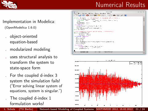
Numerical Results

Implementation in Modelica:(OpenModelica 1.6.0)

. object-orientedequation-based

. modularized modeling

. uses structural analysis totransform the system tostate-space form

. For the coupled d-index 3system the simulation fails!(“Error solving linear system ofequations, system is singular.”)

. The coupled d-index 1formulation works!


Conclusion

. If the coupled system is of d-index 1 numerical solution is fine.

. If increase of the index due to coupling occurs remodeling isrequired.

. If each subsystem is of d-index 1 a remodeling based on thetopological structure of the interconnection network might bepossible (open question).

. Redundant or inconsistent equations can be created by thecoupling resulting in non-regular systems.

. The coupling of various subsystems can result in arbitraryhigh-index DAEs and a throughout analysis is still open.


Thank you for your attention!


References

S. Bächle.Numerical Solution of Differential-Algebraic Systems Arising in Circuit Simulation.PhD thesis, Institut für Mathematik, Technische Universität Berlin, 2007.

E. Eich-Soellner and C. Führer.Numerical Methods in Multibody Dynamics.B.G. Teubner, Stuttgart, 1998.

D. Estévez-Schwarz and C. Tischendorf.Structural analysis of electric circuits and consequences for MNA.Int. J. Circuit Theory Appl., 2000, 28(2): 131-162.

M. Günther and U. Feldmann.CAD-based electric-circuit modeling in industry, I. Mathematical structure and index ofnetwork equations.Surv. Math. Ind., 1999, 8:97-129.

P. Kunkel and V. Mehrmann.Index reduction for differential-algebraic equations by minimal extension.Zeitschrift für Angewandte Mathematik und Mechanik, 2004, 84:579-597.

P. Kunkel and V. Mehrmann.Differential-Algebraic Equations — Analysis and Numerical Solution.EMS Publishing House, Zürich, Switzerland, 2006.


network-based modeling of coupled electro-mechanical systems€¦ · network-based modeling of...

Documents