near infrared camera and multi-object spectrometer ......operated by the association of universities...
TRANSCRIPT

Operated by the Association of Universities for Research in Astronomy, Inc., for the National Aeronautics and Space Administration
Space Telescope Science Institute3700 San Martin Drive
Baltimore, Maryland [email protected]
Version 11.0June, 2009
Near Infrared Camera and Multi-Object Spectrometer Instrument Handbook for Cycle 17

Send comments or corrections to:Space Telescope Science Institute
3700 San Martin DriveBaltimore, Maryland 21218
E-mail: [email protected]
User SupportFor prompt answers to questions, please contact the STScI Help Desk.
• E-mail: [email protected]
• Phone: (410) 338-1082(800) 544-8125 (U.S., toll free)
World Wide WebInformation and other resources are available on the NICMOS World WideWeb site:
• URL: http://www.stsci.edu/hst/nicmos
Revision History
CitationIn publications, refer to this document as:Viana, A., Wiklind, T., et al. 2009, “NICMOS Instrument Handbook”,Version 11.0, (Baltimore: STScI).
Version Date Editors
11.0 June 2009 A. Viana, T. Wiklind, A, Koekemoer, D. Thatte, T. Dahlen, E. Barker, R. de Jong, N. Pirzkal
10.0 December 2007 E. Barker, T. Dahlen, A. Koekemoer, L. Bergeron, R. de Jong, H. McLaugh-lin, N. Pirzkal, B. Shaw, T. Wiklind
9.0 October 2006 E. Barker, N. Pirzkal, K. Noll, S. Arribas, L. Bergeron, R. de Jong, A. Koekemoer, H. McLaughlin, T. Wiklind, C. Xu
8.0 October 2005 A. Schultz, K. Noll, E. Barker, S. Arribas, L. Bergeron, R. de Jong, S. Malho-tra, B. Mobasher, T. Wiklind, C. Xu
7.0 October 2004 K. Noll, A. Schultz, E. Roye, S. Arribas, L. Bergeron, R. de Jong, S. Malhotra, B. Mobasher, T. Wiklind, C. Xu
6.0 October 2003 E. Roye, K. Noll, S. Malhotra, D. Calzetti, S. Arribas, L. Bergeron, T. Böker, M. Dickinson, B. Mobasher, L. Petro, A. Schultz, M. Sosey, C. Xu
5.0 October 2002 S. Malhotra, L. Mazzuca, D. Calzetti, S. Arribas, L. Bergeron, T. Böker, M. Dickinson, B. Mobasher, K. Noll, L. Petro, E. Roye, A. Schultz, M. Sosey, C. Xu
4.1 May 2001 A. Schultz, S. Arribas, L. Bergeron, T. Böker, D. Calzetti, M. Dickinson, S. Holfeltz, B. Monroe, K. Noll, L. Petro, M. Sosey
4.0 May 2000 T. Böker, L. Bergeron, D. Calzetti, M. Dickinson, S. Holfeltz, B. Monroe, B. Rauscher, M. Regan, A. Sivaramakrishnan, A. Schultz, M. Sosey, A. Storrs
3.0 June 1999 D. Calzetti, L. Bergeron, T. Böker, M. Dickinson, S. Holfeltz, L. Mazzuca, B. Monroe, A. Nota, A. Sivaramakrishnan, A. Schultz, M. Sosey, A. Storrs, A. Suchkov.
2.0 July 1997 J.W. MacKenty, C. Skinner, D. Calzetti, and D.J. Axon
1.0 June 1996 D.J. Axon, D. Calzetti, J.W. MacKenty, C. Skinner

Table of ContentsAcknowledgments .................................................................... ix
Chapter 1: Introduction andGeneral Considerations...................................................1
1.1 Purpose ........................................................................................2
Document Conventions....................................................................3
1.2 Layout ..........................................................................................3
1.3 NICMOS Proposal Preparation .............................................6
1.4 The Help Desk at STScI..........................................................6
1.5 The NICMOS Instrument Team at STScI ..........................7
1.6 Supporting Information and the NICMOS Web Site ........................................................................................7
1.7 NICMOS History in Brief ......................................................7
1.8 Three-Gyro Guiding.................................................................8
1.9 Recommendations for Proposers ..........................................9
1.10 Supported and Unsupported NICMOS Capabilities .................................................................................12
Chapter 2: Overview of NICMOS.............................15
2.1 Instrument Capabilities..........................................................15
2.2 Heating, Cooling and Focus.................................................17
2.3 NICMOS Instrument Design ...............................................19
2.3.1 Physical Layout....................................................................19 2.3.2 Imaging Layout....................................................................21 2.3.3 Camera NIC1 .......................................................................22 2.3.4 Camera NIC2 .......................................................................23 2.3.5 Camera NIC3 .......................................................................23 2.3.6 Location and Orientation of Cameras .................................23
2.4 Basic Operations .....................................................................24
2.4.1 Detectors’ Characteristics and Operations...........................24
iii

iv Table of Contents
2.4.2 Comparison to CCDs ...........................................................26 2.4.3 Target Acquisition Modes ...................................................26 2.4.4 Attached Parallels ................................................................27
Chapter 3: Designing NICMOS Observations ...........................................................................29
3.1 Overview of Design Process ................................................29
3.2 APT and Aladin.......................................................................32
Chapter 4: Imaging .................................................................33
4.1 Filters and Optical Elements ................................................33
4.1.1 Nomenclature.......................................................................33 4.1.2 Out-of-Band Leaks in NICMOS Filters...............................34
4.2 Photometry................................................................................41
4.2.1 Solar Analog Absolute Standards ........................................41 4.2.2 White Dwarf Absolute Standards ........................................42 4.2.3 Photometric Throughput and Stability.................................42 4.2.4 Count Rate Dependent Non-linearity ..................................43 4.2.5 Intrapixel Sensitivity Variations ..........................................44 4.2.6 Special Situations.................................................................45
4.3 Focus History ...........................................................................48
4.4 Image Quality ..........................................................................50
4.4.1 Strehl Ratios.........................................................................50 4.4.2 NIC1 and NIC2....................................................................50 4.4.3 NIC3.....................................................................................54 4.4.4 PSF Structure .......................................................................57 4.4.5 Optical Aberrations: Coma and Astigmatism......................57 4.4.6 Field Dependence of the PSF...............................................58 4.4.7 Temporal Dependence of the PSF: HST Breathing
and Cold Mask Shifts...............................................................58
4.5 Cosmic Rays.............................................................................59
4.6 Photon and Cosmic Ray Persistence..................................60
4.7 The Infrared Background......................................................62
4.8 The “Pedestal Effect”.............................................................66

Table of Contents v
Chapter 5: Coronagraphy, Polarimetry and Grism Spectroscopy ..............................................69
5.1 Coronagraphy...........................................................................69
5.1.1 Coronagraphic Acquisitions ................................................72 5.1.2 PSF Centering ......................................................................76 5.1.3 Temporal Variations of the PSF ..........................................76 5.1.4 FGS Guiding ........................................................................77 5.1.5 Cosmic Ray Persistence.......................................................78 5.1.6 Contemporary Flat Fields ....................................................78 5.1.7 Coronagraphic Polarimetry..................................................79 5.1.8 Coronagraphic Decision Chart.............................................79
5.2 Polarimetry ...............................................................................81
5.2.1 NIC 1 and NIC2 Polarimetric Characteristics andSensitivity ................................................................................81
5.2.2 Ghost images........................................................................84 5.2.3 Observing Strategy Considerations .....................................85 5.2.4 Limiting Factors...................................................................86 5.2.5 Polarimetry Decision Chart .................................................87
5.3 Grism Spectroscopy ...............................................................89
5.3.1 Observing Strategy ..............................................................90 5.3.2 Grism Calibration ................................................................92 5.3.3 Relationship Between Wavelength and Pixel ......................92 5.3.4 Sensitivity ............................................................................93 5.3.5 Intrapixel Sensitivity............................................................96 5.3.6 Grism Decision Chart ..........................................................96
Chapter 6: NICMOS Apertures and Orientation ....................................................................99
6.1 NICMOS Aperture Definitions ...........................................99
6.2 NICMOS Coordinate System Conventions....................100
6.3 Orients......................................................................................101

vi Table of Contents
Chapter 7: NICMOS Detectors..................................103
7.1 Detector basics.......................................................................103
7.2 Detector Characteristics ......................................................105
7.2.1 Overview............................................................................105 7.2.2 Dark Current ......................................................................106 7.2.3 Flat Fields and the DQE.....................................................108 7.2.4 Read Noise .........................................................................111 7.2.5 Linearity and Saturation.....................................................112 7.2.6 Count Rate Non-Linearity .................................................113
7.3 Detector Artifacts..................................................................114
7.3.1 Shading ..............................................................................114 7.3.2 Amplifier Glow..................................................................116 7.3.3 Overexposure of NICMOS Detectors................................117 7.3.4 Electronic Bars and Bands .................................................117 7.3.5 Detector Cosmetics ............................................................118 7.3.6 "Grot".................................................................................118
Chapter 8: Detector Readout Modes ....................121
8.1 Introduction ............................................................................121
Detector Resetting as a Shutter ....................................................123
8.2 Multiple-Accumulate Mode ...............................................123
8.3 MULTIACCUM Predefined Sample Sequences(SAMP-SEQ) ...........................................................................125
8.4 Accumulate Mode.................................................................128
8.5 Read Times and Dark Current Calibration in ACCUM Mode .......................................................................130
8.6 Trade-offs Between MULTIACCUM and ACCUM ............................................................................131
8.7 Acquisition Mode .................................................................132
Chapter 9: Exposure Time Calculations ...........133
9.1 Overview: Web based NICMOS ETC.............................133
9.1.1 Instrumental Factors .........................................................135
9.2 Calculating NICMOS Imaging Sensitivities..................136
9.2.1 Calculation of Signal-to-Noise Ratio.................................136 9.2.2 Saturation and Detector Limitations ..................................138 9.2.3 Exposure Time Calculation ...............................................138

Table of Contents vii
Chapter 10: Overheads and Orbit Time Determination .......................................................143
10.1 Overview...............................................................................143
10.2 NICMOS Exposure Overheads.......................................144
10.3 Orbit Use Determination .................................................147
10.3.1 Observations in the Thermal Regime Using a Chop Pattern and MULTIACCUM.....................................147
Appendix A: Imaging Reference Material .......151
Appendix B: Flux Units and Line Lists ..............179
B.1 Infrared Flux Units................................................................179
B.1.1 Some History......................................................................179
B.2 Formulae..................................................................................181
B.2.1 Converting Between Fn and Fl ...........................................181B.2.2 Conversion Between Fluxes and Magnitudes ....................181B.2.3 Conversion Between Surface Brightness Units .................182
B.3 Look-up Tables ......................................................................182
B.4 Examples .................................................................................189
B.5 Infrared Line Lists.................................................................189
Appendix C: Bright Object Mode ...........................197
C.1 Bright Object Mode ..............................................................197
Appendix D: Techniques for Dithering, Background Measurement and Mapping ...201
D.1 Introduction ............................................................................202
D.2 Strategies For Background Subtraction...........................204
D.2.1 Compact Objects ................................................................204D.2.2 Extended Objects ...............................................................204
D.3 Chop and Dither Patterns ....................................................206
D.3.1 Dither Patterns ...................................................................208D.3.2 Chop Patterns .....................................................................209D.3.3 Combined Patterns .............................................................210D.3.4 Map Patterns ......................................................................211D.3.5 Combining Patterns and POS-TARGs...............................212D.3.6 Generic Patterns .................................................................213
D.4 Examples .................................................................................213
D.5 Types of Motions ..................................................................216

viii Table of Contents
Appendix E: The NICMOS Cooling System .........................................................................................217
E.1 The NICMOS Cooling System ..........................................217
Glossary and Acronym List...........................................221
Index ...................................................................................................227

AcknowledgmentsThe technical and operational information contained in this Handbook is
the summary of the experience gained both by members of the STScINICMOS group and by the NICMOS IDT (P.I.: Rodger Thompson, U. ofArizona) encompassing Cycle 7, Cycle 7N and Cycles 11-16. Specialthanks are due to Marcia Rieke, Glenn Schneider and Dean Hines (U. ofArizona), whose help has been instrumental in many sections of thisHandbook. We are also indebted to Wolfram Freudling (ST-ECF) for majorcontributions to the section on the NICMOS grisms.
The editors are grateful for the contributions from the past and presentmembers of the NICMOS group and members of the SSB group at STScIincluding: Santiago Arribas, Eddie Bergeron, Torsten Boeker, HowardBushouse, Daniela Calzetti, Luis Colina, Mark Dickinson, Sherie Holfeltz,David Grumm, Chris Hanley, Robert Jedrzejewski, Victoria Laidler, LisaMazzuca, Helene McLaughlin, Bahram Mobasher, Keith Noll, AntonellaNota, Adam Riess, Erin Roye, Chris Skinner, Al Schultz, AnandSivaramakrishnan, Megan Sosey, Alex Storrs, Anatoly Suchkov, Chun Xu,Wolfram Freudling (ST-ECF). We are also grateful for the technicalassistance provided by Susan Rose and Jim Younger in editing thisHandbook.
ix

x Acknowledgments

CHAPTER 1:
Introduction andGeneral Considerations
In this chapter . . .
The Near Infrared Camera and Multi-Object Spectrometer, NICMOS,provides HST with infrared imaging and spectroscopic capabilitiesbetween 0.8 and 2.5 microns. Above the earth’s atmosphere, NICMOSprovides access to this complete spectral range without hindrance fromatmospheric emission or absorption at a sensitivity and angular resolutionnot possible from the ground. The sky background for NICMOS is muchmore stable and 100 to 300 times lower in the J and H bands than forground-based telescopes (refer to Figure 4.17). It is a factor of 1.5 to 2times lower in the K band.
NICMOS, which operated from February 1997 until November 1998using an onboard exhaustible cryogen, was revived with the installation ofthe NICMOS Cooling System (NCS) during the Servicing Mission SM3B,
1.1 Purpose / 2
1.2 Layout / 3
1.3 NICMOS Proposal Preparation / 6
1.4 The Help Desk at STScI / 6
1.5 The NICMOS Instrument Team at STScI / 7
1.6 Supporting Information and the NICMOS Web Site / 7
1.7 NICMOS History in Brief / 7
1.8 Three-Gyro Guiding / 8
1.9 Recommendations for Proposers / 9
1.10 Supported and Unsupported NICMOS Capabilities / 12
1

2 Chapter 1: Introduction and General Considerations
in February 2002. The NCS provides active cooling through a series ofclosed circuit loops containing cryogenic gas.
This Handbook provides the instrument specific information needed topropose HST observations (Phase I), design accepted proposals (Phase II,in conjunction with the Phase II Proposal Instructions), and understandNICMOS in detail. The Handbook has been revised from its originalversions to include the performance with the NCS.
This chapter explains the layout of the Handbook and how to getadditional help and information through the Help Desk and STScI WorldWide Web pages. It also lists the supported capabilities of NICMOS andincludes basic recommendations on how to use the instrument.
1.1 Purpose
The NICMOS Instrument Handbook is the basic reference manual forthe Near Infrared Camera and Multi-Object Spectrometer and describes theinstrument’s properties, performance, and operations. A description of theimage reduction and calibration can be found in the NICMOS DataHandbook. The Handbooks are maintained by the NICMOS InstrumentGroup at STScI.
We designed the document to serve three purposes:
• To provide instrument-specific information for preparing observing proposals with NICMOS.
• To provide instrument-specific information to support the design of Phase II programs for accepted NICMOS proposals (in conjunction with the Phase II Proposal Instructions).
• To provide technical information about the current operation and per-formance of the instrument, which can help in understanding prob-lems and interpreting data acquired with NICMOS.
This Handbook is not meant to serve as a manual for the reduction andanalysis of data taken with NICMOS. For this, please refer to the HST DataHandbook

Layout 3
Document ConventionsThis document follows the usual STScI convention in which terms,
words, and phrases which are to be entered by the user in a literal way on aproposal are shown in a typewriter font (e.g., SAMP-SEQ=STEP16,MULTIACCUM). Names of software packages or commands (e.g.,synphot) are given in bold type.
Wavelength units in this Handbook are in microns (m) and fluxes aregiven in Janskys (Jy), unless otherwise noted.
1.2 Layout
NICMOS provides direct imaging in broad, medium, and narrow-bandfilters at a range of spatial resolutions in the near infrared from 0.8 to 2.5microns, together with broad-band imaging polarimetry, coronagraphicimaging and slitless grism spectroscopy. Figure 1.1 provides a road map tonavigating this document.
The chapters of this Handbook are as follows:
• Chapter 1: Introduction and General Considerations, describes the Handbook layout, where to find help and additional documentation, and important advice for preparing NICMOS proposals.
• Chapter 2: Overview of NICMOS, provides an introduction to the capabilities of NICMOS under NCS operations, the basic physical and imaging layout, and a summary of the detectors’ operations.
• Chapter 3: Designing NICMOS Observations, shows in tabular form the required steps for designing a NICMOS observing program, guides users through some of the technical details for choosing the optimal configuration for a given observation, and provides the reader with a “map” for the subsequent chapters.
• Chapter 4: Imaging, provides a description of NICMOS’s imaging capabilities including camera resolutions and throughputs, image quality and effects of cosmic rays. The infrared background seen by NICMOS is also described here.
• Chapter 5: Coronagraphy, Polarimetry and Grism Spectroscopy, provides detailed information on coronagraphic imaging, grism spec-troscopy, and polarimetry.
• Chapter 6: NICMOS Apertures and Orientation, describes the aper-ture definitions and the sky-projected orientation of the instrument.

4 Chapter 1: Introduction and General Considerations
• Chapter 7: NICMOS Detectors, describes the basic properties of the detectors used in the three cameras including their physical charac-teristics, capabilities and limitations. Performance descriptions are based on calibrations under NCS operations.
• Chapter 8: Detector Readout Modes, explains the data taking modes which take advantage of the non-destructive readout capabilities of the NICMOS arrays. While nearly all observers will choose to use MULTIACCUM mode, we give descriptions of other modes to help proposers/users choose the most appropriate ones for their observa-tions.
• Chapter 9: Exposure Time Calculations, provides information for performing signal-to-noise calculations, either by using pencil and paper, or using software tools that are provided on the World Wide Web (WWW).
• Chapter 10: Overheads and Orbit Time Determination, provides information to convert from a series of planned science exposures to an estimate of the number of orbits, including spacecraft and NIC-MOS overheads. This chapter applies principally to the planning of Phase I proposals.
• Appendix A: Imaging Reference Material, provides summary infor-mation and filter transmission curves for each imaging filter, ordered by camera and increasing wavelength.
• Appendix B: Flux Units and Line Lists, provides formulae and tables for the conversion of flux units, and a list of common infrared spec-tral lines.
• Appendix C: Bright Object Mode, describes the BRIGHTOBJ read-out mode.
• Appendix D: Techniques for Dithering, Background Measurement and Mapping, describes the implementation of a pre-defined set of patterns which accomplish dithering and chopping from the field of interest, and allow easy generation of large mosaic images.
• Appendix E: The NICMOS Cooling System, describes the system that has cooled NICMOS since Cycle 11.

Layout 5
Figure 1.1: Roadmap for Using the NICMOS Instrument Handbook
see NICMOS Data Handbook
Finish
Information on
Obtain Overview of NICMOSCapabilities and Operation
General Recommendations
Select Coronagraphy,Polarimetry, or Grisms &
Estimate Exposure Times
Select Imaging &Estimate Exposure Times
Detailed ExposureTime Calculations
Additional ReferenceMaterial
Start
Determine Overheads andCalculate Phase I Orbit Time
Request
Using NICMOS to MeasureBackgrounds or Make Maps?
Appendix A, B
Chapter 1
Chapter 10
Appendix D
Chapter 4, 9, Appendix A, C
Chapter 5, 6, 9
Chapter 2, 3, Appendix C
Chapter 1
Chapter 9,Web ETC
Information onNICMOS Detectors
Chapter 7, Appendix C
NICMOS Calibrations

6 Chapter 1: Introduction and General Considerations
1.3 NICMOS Proposal Preparation
The NICMOS Instrument Handbook and the current Call for Proposals(CP) should be used when assembling NICMOS Phase I Proposals. The CPprovides policy and instructions for proposing. In addition, the HST Primerprovides a basic introduction to the technical aspects of HST and itsinstruments and explains how to calculate the appropriate number of orbitsfor your Phase I observing time requests. The NICMOS InstrumentHandbook contains detailed technical information about NICMOS,describing its expected performance, and presenting suggestions for use.
If the Phase I proposal is accepted, the proposer will be asked to submita Phase II program in which the exact configurations, exposure times andsequences of observations that NICMOS and the telescope should performare specified. To assemble the Phase II program the observer is referred tothe NICMOS Instrument Handbook and to the Phase II ProposalInstructions. These instructions describe the rules and syntax that apply tothe planning and scheduling of NICMOS observations and providerelevant observatory information.
1.4 The Help Desk at STScI
STScI maintains a Help Desk. The Help Desk staff at STScI quicklyprovide answers to any HST-related topic, including questions regardingNICMOS and the proposal process. The Help Desk staff have access to allof the resources available at the Institute, and they maintain a database ofanswers so that frequently asked questions can be immediately answered.The Help Desk staff also provide STScI documentation, in either hardcopyor electronic form, including instrument science reports, instrumenthandbooks, and the like. Questions sent to the Help Desk are usuallyanswered within two working days. Commonly, the Help Desk staff willreply with the answer to a question, but occasionally they will need moretime to investigate the answer. In these cases, they will reply with anestimate of the time needed to supply a full answer.
We ask proposers to please send all initial inquiries to the Help Desk. Ifa question requires a NICMOS Instrument Scientist to answer it, the HelpDesk staff will put a NICMOS Instrument Scientist in contact with theproposer. By sending requests to the Help Desk, proposers are guaranteedthat someone will provide them with a timely response.

The NICMOS Instrument Team at STScI 7
To contact the Help Desk at STScI:
• Send e-mail (preferred method): [email protected]
• Phone: (410) 338-1082
The Space Telescope European Coordinating Facility (ST-ECF) alsomaintains a help desk. European users should generally contact the ST-ECFfor help: all other users should contact STScI. To contact the ST-ECF HelpDesk:
• Send e-mail: [email protected]
1.5 The NICMOS Instrument Team at STScI
STScI provides a team of Instrument Scientists, ScientificProgrammers, and Research & Data Analysts who support thedevelopment, operation and calibration of NICMOS. The team is alsoresponsible for supporting NICMOS users, as well as maintaining andupdating the NICMOS Instrument and Data Handbooks.
1.6 Supporting Information and the NICMOS Web Site
The NICMOS Instrument Team at STScI maintains a World Wide Webpage, as part of the STScI home page. The URL for the STScI NICMOSpage is:
http://www.stsci.edu/hst/nicmos
1.7 NICMOS History in Brief
In order to understand the list of recommendations for proposalpreparation given below, a brief history of the Instrument is presented here.A more detailed description of the NICMOS chronology, from installationon HST until its present status, is given in Chapter 2.
During its first operational period, which went from February 1997(date of installation on HST) to January 1999, NICMOS was passivelycooled by sublimating N2 ice. Science observations were obtained from thebeginning of June 1997 until mid-November 1998, during which period thecryogen kept the detectors’ temperature around 60 K, with a slow upwardtrend, from 59.5 K to ~62 K, as the N2 was sublimating. On January 3,

8 Chapter 1: Introduction and General Considerations
1999, the cryogen was completely exhausted, marking the official end ofNICMOS operations under this cooling regime. NICMOS was revived inMarch 2002 when the NICMOS Cooling System (NCS) was installed.NCS was activated and NICMOS was cooled down to the current operatingtemperature of 77.15 K.
NICMOS offers infrared capabilities in three cameras, NIC1, NIC2, andNIC3, characterized by three magnification factors (see Chapter 2). Thethree cameras had been built to be parfocal and to operate simultaneously.A few months before launch, however, the NICMOS dewar underwentthermal stresses, which made the three cameras no longer parfocal(although they still retain the capability to operate simultaneously). Evenworse, shortly after installation on HST, the NICMOS dewar developed adeformation which had two consequences: 1. It pushed the NIC3 focusoutside the range of the Pupil Alignment Mechanism (PAM); 2. It created a“heat sink”, which caused the Nitrogen ice to sublimate at a quicker pace,thus shortening the lifetime of the instrument (from the expected 4.5 yearsdown to about 2 years). A couple of months after the start of the short, theinstrument stabilized at the operating configuration which remained duringthe duration of its ‘cryogenic lifetime’ with NIC1 and NIC2 in focus andpractically parfocal, NIC3 out of focus relative to the other two camerasand with its best focus slightly outside the PAM range. During Cycle 7 andCycle 7N, two observing campaigns were organized to obtain in-focusNIC3 observations by moving the HST secondary mirror.
The current NICMOS operating configuration is nearly the same asCycle 7 and 7N: NIC1/NIC2 close to being parfocal and in focus, NIC3 isnon-parfocal with the other two cameras with the optimal focus slightly outof the PAM range. NIC3 is perfectly usable with the best achievable focus.See Chapter 4 for NIC3 operations in Cycle 11 and beyond.
1.8 Three-Gyro Guiding
We anticipate that all HST observations in Cycle 17 will be undertakenin the Three-Gyro Science Mode, providing greater scheduling flexibil-ity and greater sky coverage (at any epoch) than in Cycles 14, 15 and 16.Proposers should plan their observations accordingly, using the TargetAvailability Table in the Primer (Table 6.1) and the visibility tools on theHST Phase I Proposal Roadmap Web site.

Recommendations for Proposers 9
1.9 Recommendations for Proposers
We give here a summary of general recommendations for both Phase Iand Phase II proposal preparation. Recommendations are based ourexperience with NICMOS. However, observers are strongly advised toread the technical sections that follow in order to develop an optimalobservation strategy based on the demands of their individual scientificgoals. Also the Advisories page maintained on the NICMOS WWW siteshould be consulted for updates.
Recommendations for Phase I proposals:
• NIC1 (NIC2) offers diffraction-limited capabilities at J- (H-) band and longer wavelengths, while NIC3 offers high sensitivity (due to the lower angular resolution) with the largest field-of-view among the three cameras (see Section 2.3.2). In particular, NIC3 reaches fainter magnitudes than the other two cameras (for the same exposure time) for observations which are not limited by photon noise from source + background, i.e. where read-out or dark noise are signifi-cant. This is true for most observations of faint targets. However, the poor spatial sampling of NIC3 can limit its sensitivity for faint point sources, and also limits photometric accuracy for point sources.
• When choosing NIC3, proposers should be aware that this camera is slightly out-of-focus, with a typical loss of peak flux around 20% and a loss of encircled energy of about 10%–15% at 0.2" radius. Chapter 4 should be consulted for the detailed performance of the out-of-focus NIC3.
• The highest sensitivity gain relative to ground-based observations is at wavelengths shorter than 1.8 m. The background at J and H seen by HST is a few hundred times smaller than at ground-based obser-vatories. The background at K is only marginally better on HST, due to the telescope’s thermal emission. However, observations in the thermal regime (longward of 1.8 m) may be more advantageous with NICMOS if high angular resolution is a requirement for the sci-ence goal. Also, with NICMOS, one gains in stability of the thermal background.
• Observations of extended sources in the thermal regime (longward of 1.8 m) may need to obtain background observations as well (chop-ping off the target). Given the stability of the thermal background, however, it will not be necessary to get background measurements more frequently than once per orbit. For point sources or extended sources which do not fill the camera field-of-view, images of the thermal background can be obtained with dithering (see recommen-dations below).

10 Chapter 1: Introduction and General Considerations
• For the purpose of removing cosmic rays, photon and cosmic-ray persistence, detector artifacts, and for averaging out flat-field sensi-tivity variations, observers are strongly advised to dither an observa-tion as much as possible. This implies dividing single-orbit observations into at least three exposures and multi-orbit observa-tions into two exposures per orbit. The general advice of dithering is generally not applicable to observations of faint sources around/near bright ones. If the bright source saturates the detector, the saturated pixels will be affected by persistence; in this case, the observers have two options: 1. Not dithering, to avoid placing the faint target on the saturated pixels; 2. Dithering by large amounts (by roughly one full detector quadrant) to move away from the persistence-affected region.
• The dithering requirement poses a practical upper limit of ~1,500 seconds to the longest integration time for a single exposure. This is roughly equivalent to having 2 exposures per orbit. Observers wish-ing to detect faint targets should work out their S/N requirements by determining (e.g., with the ETC) the S/N achieved in a single expo-sure and then co-adding n exposures according to , until the desired S/N is achieved. The latter is an essential step given the large read-out noise of the NICMOS detectors.
• In the case of crowded fields, observers are advised to dither their observations with sub-pixel sampling. In post-processing, the images should be combined with the MultiDrizzle software (Fruchter, A. and Sosey, M. et al. 2009, "Multidrizzle Handbook", Version 3.0, (Balti-more, STScI)), otherwise the limiting sensitivity of NICMOS will not be reached due to PSF overlap and confusion.
• Proposers who want to use the NIC3 grisms should be aware that the spectral resolution quoted in the Handbook (R~200) is per pixel; the actual resolution, calculated over 2 pixels, is R~100.
• Observers proposing to use the NICMOS coronagraphic hole may want to consider observing the same object twice in the same orbit, or back-to-back in adjacent orbits, with an in-between roll of the space-craft for optimal PSF subtraction.
• Observers proposing to use the NICMOS coronagraphic hole may want to consider adding contemporary flat-field observations.
Recommendations for Phase II proposals:
• For fields containing faint targets only, the linear MULTIACCUM sequences (SPARS...) should be preferred. They are best suited for removing instrumental effects from the astronomical data. However, for fields containing both bright and faint sources, logarithmic
n

Recommendations for Proposers 11
sequences should be preferred (STEP...), as they offer the largest dynamic range and allow the calibration software to recover satu-rated targets.
• When designing dithering patterns, observers should take into account that the sensitivity across each detector changes by as much as a factor ~2.5 at short wavelengths and by a factor ~2 at long wave-lengths. The sensitivities used in the ETC and in this Handbook are average values across each detector. The sensitivity variations will mostly affect observers interested in the full field-of-view.
• The NIC3 PSF is undersampled and intrapixel sensitivity variations are large in this camera (see Xu, NICMOS ISR-2003-009). Photome-try on point sources can vary by >0.2 mag in J and up to 0.2 mag in H depending on the placement within a pixel. Observers are encouraged to consider sub-pixel dithering in their NIC3 observations; 4–6 dith-ering positions minimum are recommended.
• The bottom 10–15 rows of the three cameras’ fields of view are somewhat vignetted and interesting targets should not be placed in this region.
• For coronagraphic observations: coronagraphic hole movements and HST focus changes (breathing) will result in residual noise during PSF subtraction. PSF stars should be observed close in time to the primary target.
• HST absolute pointing is only good to about 1 arcsecond ( ); dithering patterns should be designed to place sci-ence targets away from the edges of the cameras by at least this amount.
1 0.33=

12 Chapter 1: Introduction and General Considerations
1.10 Supported and Unsupported NICMOS Capabilities
As was done for all the HST instruments for past Cycles, we haveestablished a set of core scientific capabilities of NICMOS which will besupported. These capabilities cover an enormous range of scienceapplications.
Supported capabilities include:
• NIC1, NIC2, and NIC3 observations in any filter or polarizer/grism. NIC3 comes “as is”, namely slightly out-of-focus (see Chapter 4 for a detailed explanation of the NIC3 capabilities).
• MULTIACCUM detector readout mode.
- The defined MULTIACCUM SAMP-SEQ exposure time sequences.- A subset of the ACCUM exposure times as defined in Chapter 8
with NREAD=1 only.
• Coronagraphic observations, including on-board target acquisitions.
Three additional capabilities are “available”, but not supported forCycle 17. The use of these capabilities requires approval from STScI anddetailed support for calibration will not be provided.
The unsupported (“available”) capabilities are:
• BRIGHTOBJ readout mode.
The use of this capability can be proposed upon consultation with aNICMOS Instrument Scientist, and is useful only for target acquisition ofextremely bright sources for coronagraphic observations. The use of thiscapability is strongly discouraged if the acquisition of a target forcoronagraphic observations can be obtained with any of the supportedcapabilities. Proposals which include this unsupported NICMOS capabilitymust include a justification of why the target acquisition cannot be donewith a supported configuration, and must justify the added risk of using anunsupported mode in terms of the science payback.
• DEFOCUS mode for de-focused observations.
Starting in Cycle 17 there will be an available observing mode forde-focused observations. This mode is classified as "available butunsupported", which means that it is available to observers who request it,but it is not supported through a full calibration program, other than basicverification that the mechanism successfully moves to the commandedde-focused position. When in use, the PAM mechanism will move to apre-determined position, leading to a decrease in the count rate. Theamount of decrease depends on the filter in use. The de-focus mode can

Supported and Unsupported NICMOS Capabilities 13
help prevent saturation when short exposures are necessitated by brightobjects, but will suffer from a degraded image quality. To implement thismode, the observer should contact the Program Coordinator.ß
• ACCUM detector readout mode
See Chapter 8 for a discussion of the problems that can be faced whenusing ACCUM mode.

CHAPTER 2:
Overview of NICMOSIn this chapter . . .
2.1 Instrument Capabilities
NICMOS, the Near Infrared Camera and Multi-Object Spectrometer, isan HST axial instrument, containing three cameras designed forsimultaneous operation. The NICMOS optics offer three adjacent but notspatially contiguous fields-of-view of different image scales. Theinstrument covers the wavelength range from 0.8 to 2.5 microns, andcontains a variety of filters, grisms, and polarizers. Each camera carries acomplement of 19 optical elements, selected through independent filterwheel mechanisms, one per camera. In order to allow operation of theNICMOS detectors and to minimize the thermal background of theinstrument, NICMOS needs to be cooled to cryogenic temperatures. Thebasic capabilities of the instrument are presented in Table 2.1.
IR imaging: NICMOS provides its highest sensitivity from 1.1 to ~2micronswhere it is superior to an 8m class telescope. Chapter 4 discussesthe overall throughput of NICMOS and the optical elements available ineach camera. The low background which HST offers between 0.8 and 2microns allows deep photometry. Our estimates of limiting sensitivities perpixel for a 5 detection in a 3,600 second integration, at an operatingtemperature of 77.15K, are given in Table 2.2. Users should note that anintegration time of 3600 sec is not practical and is for illustrative purposes.
2.1 Instrument Capabilities / 15
2.2 Heating, Cooling and Focus / 17
2.3 NICMOS Instrument Design / 19
2.4 Basic Operations / 24
15

16 Chapter 2: Overview of NICMOS
Table 2.1: Overview NICMOS Capabilities
• Grism Spectroscopy: Camera 3 has three grisms which provide a multi-object spectroscopic capability with a resolving power of R~200 per pixel over the full field of view of the camera. Their wavelength ranges are 0.8 to 1.2 microns, 1.1 to 1.9 microns, and 1.4 to 2.5 microns. Because the grisms are slitless, the spectra of spatially resolved objects are confused and multiple objects can overlap.
• Imaging Polarimetry: Three polarizing filters with pass directions of 0, 120, and 240 degrees are provided for the wavebands 0.8–1.2microns in Camera 1 and 1.9–2.1microns in Camera 2.
• Coronagraphy: A 0.3 arcsec radius occulting hole and cold mask, in the intermediate resolution Camera 2, provide a coronagraphic imag-ing capability.
Mode NIC1 NIC2 NIC3 Comments
Imaging
• FOV (arcsec) 1111 19.219.2 51.251.2
• Scale (arcsec/pixel) 0.043 0.075 0.2
• Sensitivity limit (J, H, K)a
a. Limiting magnitudes are from the NICMOS ETC (see Chapter 9). Infrared passbands (J,H,K) are defined by Bessell and Brett (1988, PASP, 100, 1134).
25.2,23.7,— 26.3,24.8,20.1 26.5,25.6,20.7 S/N = 5,texp = 3600 s
• Diffraction limit (m)
1.0 1.75 —
Grism Spectroscopy
• Type MOS slitless
• R 200 per pixel
• (m) 0.8–1.2 G096
1.1–1.9 G141
1.4–2.5 G206
• Magnitude limit (Vega H-band)a
20.5,20.4,16.6 A0V, S/N=5,texp = 3600 s
Polarimetry
• Filter angles (deg) 0, 120, 240 0, 120, 240
• (m) 0.8–1.3 1.9–2.1
Coronagraphy
• hole radius (arcsec) 0.3 cold mask

Heating, Cooling and Focus 17
Chapter 5 discusses these three special capabilities in more detail.
2.2 Heating, Cooling and Focus
NICMOS was installed onboard the HST during the second ServicingMission (SM2) in February 1997. Prior to the SM2 launch, an extensiveground testing program was executed where the nitrogen temperature waskept around 40K. Passive heat inputs caused the block of solid nitrogen toslowly warm up and it was re-cooled every 6-8 weeks. During this process,nitrogen gas froze onto the cooling coil, reducing the vapor pressure at theaft end. As the dewar warmed up, the ice at the aft end expanded, causing aslight deformation of the dewar. It was expected that this small deformationwould disappear after a fraction of the nitrogen had evaporated in orbit.The internal focus mechanism (the Pupil Alignment Mechanism PAM) wasreplaced with a version providing twice the focus range to accommodateany deviations from parfocality. After NICMOS was installed in HST, thedewar was planned to warm up to about 57 K (this high a temperature wasnever allowed to be reached during ground testing). The ice expansioncaused by this temperature increase resulted in an additional dewardeformation, to the extent that one of the (cold) optical baffles made
Table 2.2: Limiting Sensitivities in Janskys for S/N = 5 detection of a point source in a standard aperture of diameter 0.5", 0.5", and 1" for NIC1, NIC2, and NIC3, respectively, for a 3600 sec exposure.a,b.
a. S/N calculated for brightest pixel in point source image, using the NIC-MOS ETC for 77.15K temperature.b. Limiting magnitudes are from the NICMOS ETC (Chapter 9). Infrared passbands (J,H,K) are defined by Bessell and Brett (1988, PASP, 100, 1134). A0V spectrum assumed to convert between NICMOS passband flux (in Jy) and conventional, Vega-normalized JHK magnitudes.
Camera FilterBandwidth(microns)
Limiting Sensitivity
Jansky Approx. Mag.
NIC1 F110W 0.8–1.35 1.75 10-7 J 25.2
NIC1 F160W 1.4–1.8 6.26 10-7 H 23.7
NIC2 F110W 0.8–1.35 6.73 10-8 J 26.3
NIC2 F160W 1.4–1.8 2.21 10-7 H 24.8
NIC2 F237M 2.3–2.5 1.71 10-5 K 20.1
NIC3 F110W 0.8–1.35 5.49 10-8 J 26.5
NIC3 F160W 1.4–1.8 4.75 10-8 H 25.6
NIC3 F240M 2.3–2.5 9.83 10-6 K 20.7

18 Chapter 2: Overview of NICMOS
mechanical contact with the warmer vapor-cooled shield (VCS). Theresulting heat flow caused the ice to warm up even more, to about 60 K,which in turn deformed the dewar more. The motion history of NICMOSand the resulting image quality are discussed in Chapter 4 and a moredetailed history of the dewar distortion can be found at:
http://www.stsci.edu/hst/nicmos/design/history/
This unexpectedly large deformation had several undesirable effects, themost important of which are:
• The three cameras have significantly different foci, hence parallel observations are degraded. The difference between the NIC1 and NIC2 foci, however, is sufficiently small that an intermediate focus yields good quality images in both cameras.
• The NIC3 focus has moved outside of the range of the PAM. In an attempt to bring it to within the focus range, the secondary mirror was moved during two brief NIC3 campaigns in Cycle 7. During this time, HST performed exclusively NIC3 science, since no other HST instrument was in focus. Because of the extreme impact on all other instruments, no such campaigns are planned in the future. At the maximum PAM position, the degradation in terms of encircled energy at a 0.2" radius is only 5%. This is considered sufficiently small, and NIC3 will be offered “as is” in Cycle 11 and beyond.
The thermal short increased the heat flux into the inner shell (andtherefore the solid nitrogen) by a factor of ~2.5 and thereby reduced thelifetime of NICMOS from 4.5 to ~2 years. The cryogen depleted in January1999, and NICMOS was unavailable for science operation betweenJanuary 1999 and June 2002, when the NICMOS cooling system (NCS)was activated and reached expected operating temperatures. Theinstallation of the NCS, a mechanical cryocooler, re-enabled NICMOSoperation and restored infrared capability to HST. The NCS is capable ofcooling the NICMOS dewar to temperatures 75–86 K, significantly higherthan during Cycle 7. Therefore, many NICMOS parameters are differentfrom Cycle 7. Most notably, with the higher operating temperature, thedetector quantum efficiency (DQE) increased by ~30–50%.

NICMOS Instrument Design 19
Each camera can be operated in a de-focused mode, where the PAM isset to a non-optimal position relative to mechanical zero. The offsetpositions are -3mm, -5mm and -0.5mm for NIC1, NIC2 and NIC3,respectively. This mode can be used in grism and imaging modes and isuseful for increasing the efficiency when observing bright objects. Thephotons are spread over a larger area (more pixels), leading to longerexposure times before saturation is reached. In order to select the de-focusmode, the observer will need to contact the Program Coordinator.
2.3 NICMOS Instrument Design
2.3.1 Physical LayoutNICMOS is an axial bay instrument which replaced the Faint Object
Spectrograph (FOS) in the HST aft shroud during the Second HSTServicing Mission in February 1997. Its enclosure contains four majorelements: a graphite epoxy bench, the dewar, the fore-optics bench, and theelectronics boxes. The large bench serves to establish the alignment anddimensional stability between the HST optics (via the latches or fittings),the room temperature fore optics bench, and the cryogenic optics anddetectors mounted inside the dewar. The NICMOS dewar was designed touse solid nitrogen as a cryogen for a design lifetime of approximately 4.50.5 years. Cold gas vented from the dewar was used to cool the vaporcooled shield (VCS) which provides a cold environment for both the dewarand the transmissive optical elements (i.e., the filters, polarizers, andgrisms). The VCS is itself enclosed within two layers ofthermal-electrically cooled shells (TECs).
In September 2008 the NICMOS Cooling System failed to restart aftera planned temporary shut-down. The cause is believed to be the accu-mulation of water ice in the circulator pump housing. Several unsuc-cessful attempts to restart the NCS, using different procedures, weredone in the following months. In December 2008 the circulator wassuccessfully restarted but a problem with the compressor loop forcedthe NCS to be shut down once again. In January 2009 it was decided todefer further NCS restart attempts to the Servicing Mission 4. As ofApril 2009, the NCS remains shut-down. Please see the NICMOS webpage for the latest updates on the NCS status.

20 Chapter 2: Overview of NICMOS
Figure 2.1 is an overview of the NICMOS instrument; Figure 2.2 showsdetails of the dewar. The external plumbing at the dewar aft end, which wasused for the periodical recooling of the solid nitrogen during groundtesting, now forms the interface to the NCS. During SM3B, the NCS wasconnected to the bayonet fittings of the NICMOS interface plate. Thisallows the NCS to circulate cryogenic Neon gas through the cooling coilsin the dewar, thus providing the cooling power to bring the instrument intothe temperature range required for operation. The concept and workingprinciples of the NCS are discussed in Appendix E.
Figure 2.1: Instrument Overview

NICMOS Instrument Design 21
Figure 2.2: NICMOS Dewar
2.3.2 Imaging LayoutThe NICMOS fore-optics assembly is designed to correct the
spherically aberrated HST input beam. As shown in the left hand panel ofFigure 2.3 it comprises a number of distinct elements. The Pupil AlignmentMechanism (PAM) directs light from the telescope onto a re-imagingmirror, which focuses an image of the Optical Telescope Assembly (OTA)pupil onto an internal Field-Offset Mechanism (FOM) with a pupil mirrorthat provides a small offset capability (26 arcsec). An internal flat fieldsource is also included in the FOM assembly. In addition, the FOMprovides correction for conic error in the OTA pupil.
After the FOM, the Field Divider Assembly (FDA) provides threeseparate but closely-spaced imaging fields, one for each camera (right handpanel of Figure 2.3). The dewar itself contains a series of cold masks toeliminate stray IR emission from peripheral warm surfaces.
A series of relay mirrors generate different focal lengths andmagnifications for the three cameras, each of which contains a dedicated256 256 pixel HgCdTe chip that is developed from the NICMOS 3detector design. NICMOS achieves diffraction limited performance in thehigh resolution NIC1 longward of 1.0 microns, and in NIC2 longward of1.75 microns.

22 Chapter 2: Overview of NICMOS
Figure 2.3: Ray Diagrams of the NICMOS Optical Train. The left panel shows the fore-optics. The right panel shows the field divider and re-imaging optics for the three cameras.
The operation of each camera is separate from the others which meansthat filters, integration times, readout times and readout modes can bedifferent in each, even when two or three are used simultaneously. Thebasic imaging properties of each of the cameras are summarized in Table2.3.
2.3.3 Camera NIC1NIC1 offers the highest available spatial resolution with an 11 11
arcsec field of view and 43 milliarcsec sized pixels (similar to the WFC3UVIS pixel scale). The filter complement includes broad and medium bandfilters covering the spectral range from 0.8 to 1.8 microns and narrow band
Table 2.3: Basic Imaging Parameters
Parameter Camera 1 Camera 2 Camera 3
Pixel Size (arcsec) 0.043 0.075 0.2
Field of View (arcsec x arcsec) 11 11 19.2 19.2 51.2 51.2
ratio /80 /45.7 /17.2
Diffraction Limited Wavelength (m) 1.0 1.75 —
Pupil AlignmentMechanism (PAM)
reimaging
HST
Field Offset Mechanism+ Uniform Illuminator(FOM)
Corrector Mirror
Field Divider
Camera 2 Camera 1
Camera 3
Reimaging optics
Field Divider Assembly
Reimaging optics
Dewar optics includingwindows, filters & grisms,and cold masks
Assembly
Mirror

NICMOS Instrument Design 23
filters for Paschen , He I, [Fe II] 1.64m, and [S III] 0.953 m, bothon and off band. It is equipped with the short wavelength polarizers (0.8 to1.3 microns).
2.3.4 Camera NIC2NIC2 provides an intermediate spatial resolution with a 19.2 19.2
arcsec field of view and 75 milliarcsec pixels. The filters include broad andmedium band filters covering the spectral range from 0.8 to 2.45 microns.The filter set also includes filters for CO, Brackett , H2 S2 (1-0) 2.122m, Paschen , HCO2 + C2, and the long wavelength polarizers (1.9–2.1microns). Camera 2 also provides a coronagraphic hole with a 0.3 arcsecradius.
2.3.5 Camera NIC3NIC3 has the lowest spatial resolution with a large 51.2 51.2 arcsec
field of view and 200 milliarcsec pixels. It includes broad band filterscovering the spectral range 0.8 to 2.3 microns, medium band filters for theCO band (and an adjacent shorter wavelength continuum region), andnarrow band filters for H2 S2 (1-0), [Si VI] 1.962 m, Paschen-, [Fe II] 1.64 m, and He I 1.083 m. Camera 3 also contains the multi-objectspectroscopic capability of NICMOS with grisms covering the wavelengthranges 0.8–1.2 microns, 1.1–1.9 microns, and 1.4–2.5 microns.
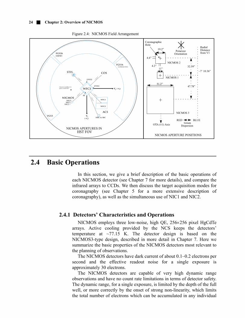
2.3.6 Location and Orientation of Cameras The placement and orientation of the NICMOS cameras in the HST
focal plane is shown in Figure 2.4. Notice that the cameras are in a straightline pointing radially outward from the center of the telescope focal plane.From the observer’s point of view the layout of NICMOS is most relevantwhen trying to plan an observation of an extended source with all threecameras simultaneously. The user must then bear in mind the relativepositions and orientations of the three cameras. The gaps between thecameras are large, and therefore getting good positioning for all camerasmay be rather difficult.
The position of the NICMOS cameras relative to the HST focal plane(i.e., the FGS frame) depends strongly on the focus position of the PAM.Since independent foci and their associated astrometric solutions aresupported for each camera, this is transparent to the observer. However, therelative positions of the NICMOS cameras in the focal plane could affectthe planning of coordinated parallels with other instruments.
24 Chapter 2: Overview of NICMOS
Figure 2.4: NICMOS Field Arrangement
2.4 Basic Operations
In this section, we give a brief description of the basic operations ofeach NICMOS detector (see Chapter 7 for more details), and compare theinfrared arrays to CCDs. We then discuss the target acquisition modes forcoronagraphy (see Chapter 5 for a more extensive description ofcoronagraphy), as well as the simultaneous use of NIC1 and NIC2.
2.4.1 Detectors’ Characteristics and OperationsNICMOS employs three low-noise, high QE, 256256 pixel HgCdTe
arrays. Active cooling provided by the NCS keeps the detectors’temperature at ~77.15 K. The detector design is based on theNICMOS3-type design, described in more detail in Chapter 7. Here wesummarize the basic properties of the NICMOS detectors most relevant tothe planning of observations.
The NICMOS detectors have dark current of about 0.1–0.2 electrons persecond and the effective readout noise for a single exposure isapproximately 30 electrons.
The NICMOS detectors are capable of very high dynamic rangeobservations and have no count rate limitations in terms of detector safety.The dynamic range, for a single exposure, is limited by the depth of the fullwell, or more correctly by the onset of strong non-linearity, which limitsthe total number of electrons which can be accumulated in any individual
NICMOS 2
NICMOS 1
NICMOS 3
OTA (v1) Axis
32.59”
47.78”51.2”
11”
19.2”
~7’ 10.36”
CoronagraphicHole
PolarizerOrientation
RadialDistancefrom V1
NICMOS APERTURE POSITIONS
RED BLUEGrism
Dispersion
4.4”
4.2”
NICMOS APERTURES INHST FOV

Basic Operations 25
pixel during an exposure. Unlike CCDs, NICMOS detectors do not have alinear regime for the accumulated signal; the low- and intermediate-countregime can be described by a quadratic curve and deviations from thisquadratic behavior is what we define as ‘strong non-linearity’. Currentestimates under NCS operations give a value of ~120,000 electrons (NIC1and NIC2) or 155,000 electrons (NIC3) for the 5% deviation fromquadratic non-linearity. This non-linearity is corrected in the standardNICMOS pipeline reduction. See Section 4.2.4 for further discussion of thetopic.
NICMOS has three detector read-out modes that may be used to takedata (see Chapter 8) plus a target acquisition mode (ACCUM,MULTIACCUM, BRIGHTOBJ, and ACQ).
The simplest read-out mode is ACCUM which provides a singleintegration on a source. A second mode, called MULTIACCUM, providesintermediate read-outs during an integration that subsequently can beanalyzed on the ground. A third mode, BRIGHTOBJ, has been designed toobserve very bright targets that would otherwise saturate the detector.BRIGHTOBJ mode reads-out a single pixel at a time. Due to the manyresets and reads required to map the array there are substantial timepenalties involved. BRIGHTOBJ mode may not be used in parallel with theother NICMOS detectors. BRIGHTOBJ mode appears to have significantlinearity problems and has not been tested, characterized, or calibratedon-orbit.
Users who require time-resolved images will have to use MULTIACCUMwhere the shortest spacing between non-destructive exposures is 0.203seconds.MULTIACCUM mode should be used for most observations. It provides
the best dynamic range and correction for cosmic rays, sincepost-observation processing of the data can make full use of the multiplereadouts of the accumulating image on the detector. Exposures longer thanabout 10 minutes should always opt for the MULTIACCUM read-out mode,
There are no bright object limitations for the NICMOS detectors.However, one must consider the persistence effect. See Section 4.6Photon and Cosmic Ray Persistence for details.
Only ACCUM, MULTIACCUM, and ACQ are supported in Cycle 11and beyond and ACCUM mode observations are strongly discouraged.

26 Chapter 2: Overview of NICMOS
because of the potentially large impact of cosmic rays. To enhance theutility of MULTIACCUM mode and to simplify the implementation,execution, and calibration of MULTIACCUM observations, a set ofMULTIACCUM sequences has been pre-defined (see Chapter 8). Theobserver, when filling out the Phase II proposal, needs only to specify thename of the sequence and the number of samples which should be obtained(which defines the total duration of the exposure).
2.4.2 Comparison to CCDsThese arrays, while they share some of the same properties as CCDs, are
not CCDs and offer their own set of advantages and difficulties. Usersunfamiliar with IR arrays should therefore not fall into the trap of treatingthem like CCDs. For convenience we summarize the main points ofcomparison:
• As with CCDs, there is read-noise (time-independent) and dark cur-rent noise (time-dependent) associated with the process of reading out the detector. The dark current associated with NICMOS arrays is quite substantial compared to that produced by the current generation of CCDs. In addition, there is an effect called shading which is a time-variable bias from the last read affecting the readout amplifiers.
• Unlike a CCD, the individual pixels of the NICMOS arrays are strictly independent and can be read non-destructively. Read-out modes have been designed which take advantage of the non-destruc-tive read capabilities of the detectors to yield the optimum sig-nal-to-noise for science observations (see Chapter 7, 8). Because the array elements are independently addressed, the NICMOS arrays do not suffer from some of the artifacts which afflict CCDs, such as charge transfer smearing and bleeding due to filling the wells. If, however, they are illuminated to saturation for sustained periods they retain a memory (persistence) of the object in the saturated pixels. This is only a concern for the photometric integrity of back to back exposures of very bright targets, as the ghost images take many min-utes, up to one hour, to be flushed from the detectors.
2.4.3 Target Acquisition ModesMost target acquisitions can be accomplished by direct pointing of the
telescope. The user should use the Guide Star Catalog-II to ensure accuratetarget coordinates. Particular care must be exercised with targets in NIC1due to its small field of view.
However, direct pointing will not be sufficient for coronagraphicobservations since the achieved precision ( ) is comparable tothe size of the coronagraphic spot (0.3"). Note that this is the HST pointingerror only. Possible uncertainties in the target coordinates need to beadded to the total uncertainty.
1 0.33=

Basic Operations 27
There are three target acquisition options for coronagraphicobservations, which are extensively discussed in Chapter 5:
• On-board acquisition (Mode-2 Acquisition). This commands NICMOS to obtain an image of the target and rapidly position the brightest source in a restricted field of view behind the coronagraphic hole. This is one of the pre-defined acquisition modes in the Phase II proposals (ACQ mode).
• The RE-USE TARGET OFFSET special requirement can be used to accomplish a positioning relative to an early acquisition image.
• A real time acquisition (INT-ACQ) can be obtained, although this is costly in spacecraft time and is a limited resource.
While ACQ mode is restricted to coronagraphic observations in Camera2, the last two target acquisition modes may be useful for positioningtargets where higher than normal (1–2 arcsec) accuracy is required (e.g.,crowded field grism exposures).
2.4.4 Attached ParallelsWhile the three NICMOS cameras are no longer at a common focus,
under many circumstances it is desirable to obtain data simultaneously inmultiple cameras.
Although some programs by their nature do not require more than onecamera (e.g., studies of isolated compact objects), observers maynonetheless add exposures from the other camera to their proposals inorder to obtain the maximum amount of NICMOS data consistent withefficiently accomplishing their primary science program. InternalNICMOS parallel observations obtained together with primary scienceobservations will be known as coordinated parallels and will be deliveredto the prime program’s observer and will have the usual proprietary period.
The foci of Cameras 1 and 2 are close enough that they can be usedsimultaneously, whereas Camera 3 should be used by itself.

CHAPTER 3:
Designing NICMOSObservations
In this chapter. ..
3.1 Overview of Design Process
In the preceding chapters, we provided an overview of the scientificcapabilities of NICMOS and the basic layout and operation of theinstrument. Subsequent chapters will provide detailed information aboutthe performance and operation of the instrument. In this chapter, we brieflydescribe the conceptual steps which need to be taken when designing aNICMOS observing proposal. The purpose of this description is to referproposers to the relevant Chapters across the Handbook. The basicsequence of steps in defining a NICMOS observation are shown in a flowdiagram in Figure 3.1, and are:
• Identify the science requirements and select the basic NICMOS con-figuration to support those requirements (e.g., imaging, polarimetry, coronagraphy). Select the appropriate camera, NIC1, NIC2 or NIC3 depending on needs and field of view. Please refer to the detailed accounts given in Chapter 4 and Chapter 5.
• Select the wavelength region of interest and determine if the observa-tions will be Background or Read-Noise limited using the Exposure Time Calculator, which is available on the STScI NICMOS Web page (see also Chapter 9 and Appendix A).
3.1 Overview of Design Process / 29
3.2 APT and Aladin / 32
29

30 Chapter 3: Designing NICMOS Observations
• Establish which MULTIACCUM sequence to use. Detailed descrip-tions of these are provided in Chapter 8. This does not need to be specified in a Phase I proposal. However, if a readout mode other than MULTIACCUM is required, this should be justified in the Phase I proposal.
• Estimate the exposure time to achieve the required signal to noise ratio and check feasibility (i.e., saturation limits). The Exposure Time Calculator (ETC) should be used to determine exposure time require-ments and assess whether the exposure is close to the brightness and dynamic range limitations of the detectors (see Chapter 9).
• If necessary, a chop and dither pattern should be chosen for better spatial sampling, to measure the background or to enable mapping, and to mitigate bad pixels. See Appendix D.
• If coronagraphic observations are proposed, additional target acquisi-tion exposures will be required to center the target in the aperture to the accuracy required for the scientific goal (e.g., the proposer may wish to center the nucleus of a galaxy in a crowded field behind the coronagraphic spot). The target acquisition overheads must be included in the accounting of orbits.
• Calculate the total number of orbits required, taking into account the overheads. In this, the final step, all the exposures (science and non-science, alike) are combined into orbits, using tabulated over-heads, and the total number of orbits required are computed. Chapter 10 should be used for performing this step.

Overview of Design Process 31
Figure 3.1: Specifying a NICMOS Observation
Chapter 5, 9
Chapter 5, 9
Chapter 9
Chapter 9
Appendix D
Chapter 5, 9
Chapter 5, 9
Chapter 4Chapter 5
Chapter 5 Chapter 5
Cam 1 Cam 2 Cam 2Cam 3
Science Mode?
Polarimetry ImagingCoronagraphyGrism
Spectroscopy
Camera withRequired Filter?
Acq Image
Broad Band
CrowdedField?
Narrow Band
Resolutionor Field?
Pick Grism
EstimateOverheads and Orbits
DesignOrients
Submit Proposal
Do At least 290 degrees apart
Short LongResolution Field
Iterate
YES
NO
ExposureTimes
CheckSaturation
Iterate
ExposureTimes
CheckSaturation
Iterate
ExposureTimes
CheckSaturation
Cam 2Cam 1Cam 2Cam 1 Cam 3
Long or
Short?
PickMosaic/Background
Pattern
Cam 3
Chapter 5Pick Filter
Appendix D
Chapter 10

32 Chapter 3: Designing NICMOS Observations
3.2 APT and Aladin
The Astronomer’s Proposal Tool (APT) is used to design HSTobservations. A new tool based on the Aladin Sky Atlas Interface isavailable to visually inspect fields and objects. This tool gives us manyoptions for future enhancements, and brings a variety of benefits to usersincluding access to a wide variety of images and catalogs, as well as manycapabilities for displaying and manipulating images. Detailed informationabout the Aladin based tool can be found on the APT Web page:
http://apt.stsci.edu.

CHAPTER 4:
ImagingIn this chapter...
4.1 Filters and Optical Elements
In total, there are 32 different filters, three grisms, and two sets of threepolarizers available for NICMOS. Each camera has 20 filter positions on asingle filter wheel: 19 filters and one blank. As a result, not all filters areavailable in all cameras. Moreover, the specialized optical elements, suchas the polarizers and grisms, cannot be crossed with other filters, and canonly be used in fixed bands. In general, the filters have been located in away which best utilizes the characteristics of NICMOS. Therefore atshorter wavelengths, the most important narrow band filters are located inNIC1 so that the diffraction limited performance can be maintainedwherever possible, while those in NIC2 have been selected to workprimarily in the longer wavelength range where it will also deliverdiffraction limited imaging.
4.1.1 NomenclatureFollowing the traditional HST naming convention, the name of each
optical element starts with a letter or group of letters identifying what kind
4.1 Filters and Optical Elements / 33
4.2 Photometry / 41
4.3 Focus History / 48
4.4 Image Quality / 50
4.5 Cosmic Rays / 59
4.6 Photon and Cosmic Ray Persistence / 60
4.7 The Infrared Background / 62
4.8 The “Pedestal Effect” / 66
33

34 Chapter 4: Imaging
of element it is: filters start with an “F”, grisms with a “G”, and polarizerswith “POL”. Following the initial letter(s) is a number which, in the case offilters, identifies its approximate central wavelength in microns, e.g.,F095N implies a central wavelength of 0.95 microns. A trailing letteridentifies the filter width, with “W” for wide, “M” for medium and “N” fornarrow. In the case of grisms, the initial “G” is followed by a number whichgives the center of the free-spectral range of the element, e.g., G206. Forthe polarizers, a somewhat different notation is used, with the initial “POL”being followed by a number which gives the PA of the principal axis of thepolarizer in degrees, and a trailing letter identifying the wavelength range itcan be used in, which is either “S” for short (0.8-1.3 microns) or “L” forlong (1.9-2.1 microns).
Tables 4.1 through 4.3 list the available filters and provide an initialgeneral description of each, starting with NIC1 and working down inspatial resolution to NIC3. Figures 4.1 through 4.3 show the effectivethroughput curves of all of the NICMOS filters for cameras NIC1, NIC2,and NIC3, respectively, which include the filter transmission convolvedwith the OTA, NICMOS foreoptics, and detector response. Appendix Aprovides further details and the individual filter throughput curves.
4.1.2 Out-of-Band Leaks in NICMOS FiltersIn order to make use of the high spatial resolution of HST, many
observers expect to use NICMOS to observe very red objects (e.g.,protostars) at relatively short wavelengths. These objects have very loweffective color temperatures. Thus, the flux of such objects at 2.5 micronsis expected to be orders of magnitude larger than their flux at desiredwavelengths. In such a case, exceptionally good out-of-band blocking isrequired from the filter since out-of-band filter leaks could potentially havea detrimental impact on photometry. We have, therefore, investigatedwhether any of the NICMOS filters show evidence for out-of-band levels.The results indicate that actual red leaks were insignificant or non-existent.

Filters and Optical Elements 35
Table 4.1: NIC 1 Filters.
NameCentral
Wavelength (m)Wavelength range (m)
Comment
Blank N/A N/A Blank
F110W 1.025 0.8–1.4
F140W 1.3 0.8–1.8 Broad Band
F160W 1.55 1.4–1.8
F090M 0.9 0.8-1.0
F110M 1.1 1.0–1.2
F145M 1.45 1.35–1.55 Water
F165M 1.6 1.54–1.74
F170M 1.7 1.6–1.8
F095N 0.953 1% [S III]
F097N 0.97 1% [S III] continuum
F108N 1.083 1% He I
F113N 1.13 1% He I continuum
F164N 1.644 1% [Fe II]
F166N 1.66 1% [Fe II] continuum
F187N 1.87 1% Paschen
F190N 1.90 1% Paschen continuum
POL0S 1.1 0.8–1.3 Short Polarizer
POL120S 1.1 0.8–1.3 Short Polarizer
POL240S 1.1 0.8–1.3 ShortPolarizer

36 Chapter 4: Imaging
Figure 4.1: Filters for NIC 1 (at 78 K).
NIC 1 Wide Band Filters
0.8 1.0 1.2 1.4 1.6 1.8 2.0Wavelength (microns)
0.00
0.05
0.10
0.15
0.20
0.25
0.30T
otal
Thr
ough
put
F110W
F140W
F160W
NIC 1 Medium Band Filters
0.8 1.0 1.2 1.4 1.6 1.8 2.0Wavelength (microns)
0.00
0.05
0.10
0.15
0.20
0.25
0.30
Tot
al T
hrou
ghpu
t
F090M
F110M
F145M
F165M
F170M
NIC 1 Narrow Band Filters
0.8 1.0 1.2 1.4 1.6 1.8 2.0Wavelength (microns)
0.00
0.05
0.10
0.15
0.20
0.25
0.30
Tot
al T
hrou
ghpu
t
F095NF097N F108N
F113N
F164NF166N
F187NF190N

Filters and Optical Elements 37
Table 4.2: NIC 2 Filters.
NameCentral
Wavelength (m)Wavelength range (m)
Comment
Blank N/A N/A Blank
F110W 1.1 0.8–1.4
F160W 1.6 1.4–1.8 Minimum background
F187W 1.875 1.75–2.0 Broad
F205W 1.9 1.75–2.35 Broad Band
F165M 1.7 1.54–1.75 Planetary continuum
F171M 1.715 1.68–1.76 HCO2 and C2 continuum
F180M 1.80 1.76–1.83 HCO2 and C2 bands
F204M 2.04 1.98–2.08 Methane imaging
F207M 2.1 2.01–2.16
F222M 2.3 2.15–2.29 CO continuum
F237M 2.375 2.29–2.44 CO
F187N 1.87 1% Paschen
F190N 1.9 1% Paschen continuum
F212N 2.121 1% H2
F215N 2.15 1% H2 and Br continuum
F216N 2.165 1% Brackett
POL0L 2.05 1.89–2.1 Longpolarizer
POL120L 2.05 1.89–2.1 Long polarizer
POL240L 2.05 1.89–2.1 Long polarizer

38 Chapter 4: Imaging
Figure 4.2: Filters for NIC 2 (at 78 K).
NIC 2 Wide Band Filters
1.0 1.5 2.0 2.5Wavelength (microns)
0.00
0.10
0.20
0.30
0.40T
otal
Thr
ough
put
F110W
F160WF187W
F205W
NIC 2 Medium Band Filters
1.0 1.5 2.0 2.5Wavelength (microns)
0.00
0.10
0.20
0.30
0.40
Tot
al T
hrou
ghpu
t
F165MF171M
F180M F204MF207M
F222MF237M
NIC 2 Narrow Band Filters
1.0 1.5 2.0 2.5Wavelength (microns)
0.00
0.10
0.20
0.30
0.40
Tot
al T
hrou
ghpu
t
F187NF187NF190N F212N
F215NF216N

Filters and Optical Elements 39
Table 4.3: NIC 3 Filters.
NameCentral Wavelength
(m)Wavelength range (m)
Comment
Blank N/A N/A Blank
F110W 1.1 0.8–1.4
F150W 1.5 1.1–1.9 Grism B continuum
F160W 1.6 1.4–1.8 Minimum background
F175W 1.75 1.2–2.3
F222M 2.3 2.15–2.28 CO continuum
F240M 2.4 2.3–2.5 CO band
F108N 1.0830 1% He I
F113N 1.13 1% He I continuum
F164N 1.644 1% [Fe II]
F166N 1.66 1% [Fe II] continuum
F187N 1.875 1% Paschen
F190N 1.9 1% Paschen continuum
F196N 1.962 1% [Si VI]
F200N 2.0 1% [Si VI] continuum
F212N 2.121 1% H2
F215N 2.15 1% H2 continuum
G096 0.9673 0.8–1.2 GRISM A
G141 1.414 1.1–1.9 GRISM B
G206 2.067 1.4–2.5 GRISM C

40 Chapter 4: Imaging
Figure 4.3: Filters for NIC 3 (at 78 K).
NIC 3 Wide Band Filters
1.0 1.5 2.0 2.5Wavelength (microns)
0.00
0.10
0.20
0.30
0.40T
otal
Thr
ough
put
F110W
F150WF160W
F175W
NIC 3 Medium Band Filters
1.0 1.5 2.0 2.5Wavelength (microns)
0.00
0.10
0.20
0.30
0.40
Tot
al T
hrou
ghpu
t F222M
F240M
NIC 3 Narrow Band Filters
1.0 1.5 2.0 2.5Wavelength (microns)
0.00
0.10
0.20
0.30
0.40
Tot
al T
hrou
ghpu
t
F108NF113N
F164NF166N
F187NF190N
F196NF200N
F212NF215N

Photometry 41
4.2 Photometry
Ground-based near-infrared observations are limited to a set oftransparent atmospheric windows, while NICMOS suffers no suchrestrictions. For this reason, faint flux standards with continuous, empiricalspectrophotometry throughout the 0.8 m < < 2.5 m range were createdusing the NICMOS grism mode in combination with spectral models. Theabsolute flux calibration of NICMOS has been calculated usingobservations of stars for which reliable spectral models, normalized byground-based photometry in the optical, are available. Two types of fluxstandards have been observed: pure hydrogen white dwarfs, and solaranalog stars. Grism sensitivity is determined directly from flat-fieldcorrected spectra of these stars using their known spectral energydistributions. Filter sensitivities are calculated from imaging measurementsaccording to the synthetic photometry procedure detailed in Koornneef andCoole (1981, ApJ, 247, 860). Since the pipeline calibration cannot utilizecolor information, the headers of reduced data contain the calibrationconstant that specifies the equivalent count rate for a spectral energydistribution that is constant with wavelength. For convenience, thiscalibration constant appears twice, once in Jansky units and once inerg/s/cm2/Angstrom units.
4.2.1 Solar Analog Absolute StandardsFor calibration using solar analogs, a reference spectrum of the Sun is
normalized to the flux levels of the NICMOS standards at opticalwavelengths. This continuous spectral model is then integrated through thetotal system throughput function for a given bandpass (including filter,detector, instrument and telescope optics), and the integral flux iscompared to the measured count rate from the star in observations throughthat filter to derive the flux calibration constants. The absolute fluxaccuracy achieved by this method relies on two assumptions:
1. that the calibrated reference spectrum of the Sun is known with anuncertainty of a few percent (Colina, Bohlin and Castelli, 1996; Boh-lin 2007, ASPC, 364, 315), and
2. that the near-infrared spectra of the solar analogs are nearly identicalto that of the Sun.
In the past, this method was used to determine the absolute calibrationof near-infrared photometry at ground-based observatories. In these cases,the absolute calibration accuracy was estimated to be at least 5%, and forsome bands 2% to 3% (Campins, Rieke and Lebofsky, 1985).

42 Chapter 4: Imaging
Ground-based photometry by Persson et al. (1998, AJ, 116, 2475) ofseveral solar analog stars used in the NICMOS calibration program hasshown that the stars P330E and P177D (see Bohlin, Dickinson & Calzetti2001, AJ, 112, 2118; Colina & Bohlin 1997, AJ, 113, 1138; Colina, Bohlin& Castelli 1996, AJ, 112, 307) are most closely matched to the colors ofthe Sun, and are thus most suitable for NICMOS photometric calibration.P330E is the primary NICMOS solar analog standard for photometriccalibration.
4.2.2 White Dwarf Absolute StandardsPure hydrogen white dwarfs are useful calibration standards because
their spectral energy distributions can be accurately modeled from the UVthrough the near-IR (Bohlin, Dickinson & Calzetti 2001, AJ, 112, 2118;Bohlin 1996, AJ, 111, 1743; Bohlin, Colina & Finley 1995, AJ, 110, 1316).The star G191B2B has therefore served as a primary calibration standardfor several HST instruments and was selected for NICMOS observationalong with another star, GD153. Using the most up-to-date white dwarfatmosphere models, normalized to the most accurate STIS optical/UVspectra of G191B2B, Bohlin, Dickinson & Calzetti (2001) find satisfactoryagreement between the white dwarf and solar analog stars for NICMOSphotometric calibration.
4.2.3 Photometric Throughput and Stability During Cycle 7, NICMOS throughput (i.e. photoelectrons per second
detected from a source with given flux) was generally within 20% ofpre-launch expectations in all observing modes. At the new, warmertemperature under NCS operations, the detector quantum efficiency ishigher at all wavelengths, with the largest improvements at shorterwavelengths. Hence, the photometric zeropoints are significantly differentwith the NCS in operation compared with Cycle 7. The latest zeropointsare always given at the NICMOS Photometry Web page available at:
http://www.stsci.edu/hst/nicmos/performance/photometry.
The photometric stability of NIC1 and NIC2 in Cycle 7 was monitoredonce a month, and more frequently near the end of the NICMOS Cryogenlifetime. Observations of the solar analog P330E were taken through asubset of filters (5 for NIC1, 6 for NIC2) covering the entire wavelengthrange of the NICMOS cameras, and dithered through three or fourpointings. NIC3 has also been monitored in a similar fashion, althoughonly two filters were used for part of the instrument’s lifetime. For mostfilters and cameras the zeropoints have been stable to within 3%throughout the lifetime of the instrument, although in Cycle 7 there was asmall secular drift as the instrument temperature changed.

Photometry 43
The monitoring program continued in Cycle 11 and beyond after theNCS was installed. Four filters in each of the cameras were monitoredusing solar analog P330E. With the switch to Two Gyro Mode in Cycle 14the white dwarf standard G191B2B was added to the monitoring programto ensure year-round coverage. In the five years since the NCS installationin 2002, there has been a decrease on the order of 1% in sensitivity in NIC2for all filters. For the other cameras, a similar effect may be present, butthis is hard to confirm due to the larger noise in photometry for thesecameras. Evidence that this effect involves all three cameras is, however,given by the flat-field monitoring (see Section 7.2.3). No satisfactoryexplanation has yet been found for this decrease in sensitivity. However,the change in sensitivity is consistent with a drift in detector temperaturewith time (see Dahlen, NICMOS ISR-2007-002).
4.2.4 Count Rate Dependent Non-linearityThe NICMOS team has determined that NICMOS has a significant
count rate dependent non-linearity that also depends on wavelength. This isa different nonlinearity from the well-known total count dependentnon-linearity. The non-linearity amounts to a 0.050.10 mag/dex offset inincident flux for the shortest wavelength (F090M and F110W), about 0.03mag/dex at F160W and less than that at longer wavelengths (see Figure4.4). Objects fainter than the NICMOS standard stars of about 12thmagnitude will be measured too faint, objects that are brighter than ourstandards will seem too bright. The effect depends entirely on the incomingflux rate, so any objects fainter than the night sky (or on top of a brightobject) will have a non-linearity offset determined by the background flux(Shaw, NICMOS ISR-2008-003). This means that the maximum offsets ondark sky backgrounds at F110W are about 0.25 mag in NIC1 and NIC2,and about 0.16 mag in NIC3 (de Jong, NICMOS-ISR 2006-001). Softwarehas been developed to linearize the counts in imaging observations (deJong, NICMOS ISR-2006-003). More details on the effect and how tocorrect for it can be found at:
http://www.stsci.edu/hst/nicmos/performance/anomalies/nonlinearity.html.

44 Chapter 4: Imaging
Figure 4.4: Wavelength dependent non-linearity amounts for all three cameras.
4.2.5 Intrapixel Sensitivity VariationsThe response of a pixel in the NICMOS detectors to light from an
unresolved source varies with the positioning of the source within the pixeldue to low sensitivity at the pixel’s edges and dead zones between pixels.The interpixel sensitivity was found to be an important effect and it variesby as much as 30%. This effect has no impact on observations of resolvedsources, and little effect on well-sampled point sources (e.g. observationswith NIC1 and NIC2 through most filters). However in NIC3, pointsources are badly under-sampled, especially at short wavelengths wherethe telescope diffraction limit is much smaller than the NIC3 pixel size.Therefore, object counts may vary by as much as 30% depending on thewavelength positioning of a star within a pixel. Well-dithered exposureswill average out this effect, but NIC3 observations of stars with few ditherpositions can have significant uncertainties which may limit the achievablequality of point source photometry.
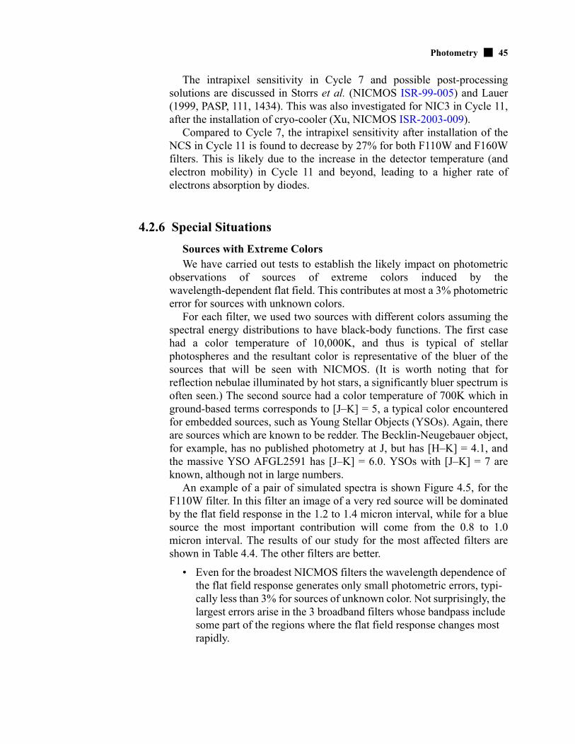
Photometry 45
The intrapixel sensitivity in Cycle 7 and possible post-processingsolutions are discussed in Storrs et al. (NICMOS ISR-99-005) and Lauer(1999, PASP, 111, 1434). This was also investigated for NIC3 in Cycle 11,after the installation of cryo-cooler (Xu, NICMOS ISR-2003-009).
Compared to Cycle 7, the intrapixel sensitivity after installation of theNCS in Cycle 11 is found to decrease by 27% for both F110W and F160Wfilters. This is likely due to the increase in the detector temperature (andelectron mobility) in Cycle 11 and beyond, leading to a higher rate ofelectrons absorption by diodes.
4.2.6 Special Situations
Sources with Extreme ColorsWe have carried out tests to establish the likely impact on photometric
observations of sources of extreme colors induced by thewavelength-dependent flat field. This contributes at most a 3% photometricerror for sources with unknown colors.
For each filter, we used two sources with different colors assuming thespectral energy distributions to have black-body functions. The first casehad a color temperature of 10,000K, and thus is typical of stellarphotospheres and the resultant color is representative of the bluer of thesources that will be seen with NICMOS. (It is worth noting that forreflection nebulae illuminated by hot stars, a significantly bluer spectrum isoften seen.) The second source had a color temperature of 700K which inground-based terms corresponds to [J–K] = 5, a typical color encounteredfor embedded sources, such as Young Stellar Objects (YSOs). Again, thereare sources which are known to be redder. The Becklin-Neugebauer object,for example, has no published photometry at J, but has [H–K] = 4.1, andthe massive YSO AFGL2591 has [J–K] = 6.0. YSOs with [J–K] = 7 areknown, although not in large numbers.
An example of a pair of simulated spectra is shown Figure 4.5, for theF110W filter. In this filter an image of a very red source will be dominatedby the flat field response in the 1.2 to 1.4 micron interval, while for a bluesource the most important contribution will come from the 0.8 to 1.0micron interval. The results of our study for the most affected filters areshown in Table 4.4. The other filters are better.
• Even for the broadest NICMOS filters the wavelength dependence of the flat field response generates only small photometric errors, typi-cally less than 3% for sources of unknown color. Not surprisingly, the largest errors arise in the 3 broadband filters whose bandpass include some part of the regions where the flat field response changes most rapidly.

46 Chapter 4: Imaging
• The same results hold true even for filters at the most extreme wave-lengths (e.g., F090M, F222M and F240M) because of their small bandwidth.
• It will probably be difficult to obtain photometry to better than the limits shown in Table 4.4 for the F090M, F110W, F140W, F205W and F240M filters, and observers requiring higher accuracy should contact the Help Desk at STScI for guidance.
• These errors can probably be corrected if more accurate photometry is needed, by taking multi-wavelength observations and using an iter-ative correction technique.
• For observers requiring high precision photometry, these represent non-trivial limits beyond which it will not be possible to venture without obtaining multi-wavelength images. In order to obtain 1% precision using the F110W filter, for instance, observers should observe at least in another wavelength. The color information derived from the pair (or group) of images could then be used to construct a more appropriate flat field image, which could then be applied to improve the color information.
Table 4.4: Photometric Errors for Selected Filters.
Filter Error (percent)10,000K model 700K model
F090M <0.1 1.9
F110W 1.1 2.9
F140W 0.7 3.1
F160W <0.1 0.3
F187W <0.1 0.3
F205W 0.4 2.1
F222W <0.1 0.1
F240M 1 0.9

Photometry 47
Figure 4.5: Detected Source Spectrum. These are for sources with color temperatures of 700K (solid line) and 10,000K (dashed line). It is easy to see that the detected image will be dominated by the flat field response in the 1.2-1.4m region for a 700K source, while for a 10,000K source the detected image will be affected by the flat field response throughout the filter bandpass.
Extended Sources with Extreme Spatial ColorVariationsSo far, the analysis has been limited to point sources, but some mention
should be made of the situation for extended objects. A good example isthe YSO AFGL2591. This has an extremely red core of [J–K] = 6, and isentirely undetected optically. However, it also has a large IR nebula whichis quite prominent at J and K, and in the red visual region, but much fainterat L, and which is probably a reflection nebula. Spatially, the nebula hashighly variable color, some parts of it having fairly neutral or even slightlyblue colors in the NICMOS waveband, while other parts are extremely red.Obtaining very accurate measurements of the color of such a sourcerequires the use of images at more than one wavelength and an iterativetool of the kind described earlier. A further example of this kind ofcomplicated object is the prototypical post-AGB object CRL2688, theCygnus Egg Nebula, which has an extremely blue bipolar reflection nebulasurrounding an extremely red core. Techniques which require very accuratemeasurements of the surface brightness of extended objects, such as thebrightness fluctuation technique for distant galaxies, will need to beapplied with care given to the photometric uncertainties such as thosediscussed here.

48 Chapter 4: Imaging
Creating Color-Dependent Flat FieldsNICMOS ISR-99-002 describes two methods for creating
color-dependent flat fields. We have included programs and calibrationfiles for making these flat fields in the software part of the Web site. Oneway of approaching the problem is to make monochromatic flats by doinga linear least squares fit to several narrowband (and, if necessary forincreased wavelength coverage) medium band flats, for each pixel. Theslope and intercept images that result from such a fit can be used todetermine the detector response to a monochromatic source. This methodworks best if the desired wavelength is within the range covered by theobserved flats; extrapolation with this method gives questionable results.
If the source spectrum is known, a composite flat made from theweighted sum of the narrowband flats in the passband of the observedimage can be made. The IRAF script, interflat.cl, uses an input spectrumand the calibration database in STSDAS to compute composite flats. Thisscript is downloadable from:
http://www.stsci.edu/hst/nicmos/tools/colorflat_intro.html.
If you have a variety of sources in your image you may want to makeseveral flat fields and apply them to regions defined by some criterion, likecolor as defined by a couple of narrowband images on either side of thebroadband image.
4.3 Focus History
The Pupil Alignment Mechanism (PAM) consists of an adjustablemirror in the NICMOS optical train that can be moved to make smallcorrections to the NICMOS focus and serves to properly position the pupilimage of the telescope primary mirror onto the corrective optic. Themotion of the PAM is limited to 10mm from its zero position. TheNICMOS cameras were designed to share a common focus with the PAMclose to its zero position. In the current state of the dewar, NIC1 and NIC2can each be focused within the range of the PAM. NIC3, however, cannotbe entirely focused by motions of the PAM alone and remains slightly outof focus although still scientifically usable (see next section).
The focus positions of all three NICMOS cameras have changed sincelaunch due to motion in the dewar. The positions are measured byobservations of stars over a range of focus settings on a frequent basis. Thefocus history since shortly after launch is shown in Figure 4.6. The focusposition is given for the detector center. The focus variation across thecamera’s field of view is ~1.5 mm in PAM space in NIC2, and about half ofthat in NIC1. The two largest focus excursions, on January 12 and June 4,1998, are due to the secondary mirror reset used to place NIC3 in focusduring NIC3 campaigns. A noticeable improvement in NIC3 focus

Focus History 49
occurred after December 17, 1997, when the FOM had been tilted by 16arcsec to reduce vignetting in that camera.
After installation of the NCS the PAM has been positioned to give thebest focus for NIC1 and NIC2. This position has proven to be quite stablefor NIC1 and NIC2. No additional special focus campaigns for NIC3 areplanned. For more information, please see the NICMOS Focus Web page.
Starting in Cycle 17 there will be an available observing mode calledDEFOCUS for de-focused observations. This mode is classified as"available but unsupported", which means that observers can request it, butthe mode is not supported through a full calibration program, other thanbasic verification that the mechanism successfully moves to thecommanded de-focused position. When in use, the PAM mechanism willmove to a pre-determined position, leading to a decrease in the count rate.The amount of decrease depends on the filter in use. The de-focus modecan help prevent saturation when short exposures are necessitated by brightobjects, but will suffer from a degraded image quality. To implement thismode, the observer should contact the Program Coordinator.
Figure 4.6: NICMOS Focus History as of 4 July 2007 (focus at the detector center).

50 Chapter 4: Imaging
4.4 Image Quality
4.4.1 Strehl RatiosThe high image quality of NICMOS is summarized by the Stroll ratio of
the PSF, which is defined as the ratio of the observed-to-perfect PSF peakfluxes. Table 4.5 lists the Stroll ratios for representative filters in all threeNICMOS cameras (courtesy of John Krist, STScI). The ratio is very high,between 0.8 and 0.9 for NICMOS images, at all wavelengths and in allCameras at their optimal focus. For more information see Seconder et al.2008 "Domains of Observability in the Near_Infrared with HST/NICMOSand AO Augmented Large Ground-Based Telescopes"
For NIC3, the quoted Strehl ratio is for optimal focus measurementsobtained during the Cycle 7 & 7N campaigns.
4.4.2 NIC1 and NIC2The changes in dewar geometry leading to the degraded focus in NIC3
have also affected NIC1 and NIC2. By measuring the PSFs of stars at aseries of PAM positions it was determined that the optimal focus for NIC1occurred for a PAM position of ~ +1.8 mm and the optimal focus for NIC2at ~ 0.2 mm after the installation of NCS in 2002. This difference issignificant enough that NIC1 and NIC2 are not considered to be parfocal.However, the NIC1 and NIC2 foci are still sufficiently close that theintermediate focus position between the two cameras, NIC1-2, has beendefined for simultaneous observations. The compromise focus position hasbeen chosen to share the waveforms error equally between NIC1 andNIC2. The image degradation induced by this compromise focus is smallerthan a few percent in each camera, and negligible for most purposes. Mostusers will find this focus sufficient to reach their scientific goals whenusing both cameras. Additionally, a separate PAM position at the optimalfocus is defined and maintained for each camera.
Table 4.5: NICMOS Strehl Ratios
Filter NIC1 NIC2 NIC3
F110W 0.91 0.89 0.84
F160W --- 0.90 0.87
F222M --- 0.90 0.92

Image Quality 51
The encircled energy profiles for NIC1 and NIC2 at representativewavelengths are shown in Figures 4.7 through 4.11.
Figure 4.7: Encircled Energy for NIC1, F110W.

52 Chapter 4: Imaging
Figure 4.8: Encircled Energy for NIC1, F160W.
Figure 4.9: Encircled Energy for NIC2, F110W.

Image Quality 53
Figure 4.10: Encircled Energy for NIC2, F160W.
Figure 4.11: Encircled Energy for NIC2, F222M.

54 Chapter 4: Imaging
Vignetting in NIC1 and NIC2The lateral shifts of the NICMOS dewar have resulted in vignetting in
all three cameras. The primary source of the vignetting is a slightmisalignment of the FDA mask. Relatively small losses in throughput areobserved at the bottom ~ 15 rows of both NIC1 and NIC2 as shown inFigure 4.12, but a more substantial vignetting is seen in NIC3.
Figure 4.12 shows the column plot of the ratio of an in-flight flat field toa pre-launch flat field for NIC1 and NIC2 for the F110W filter. Theapproximately 10% decrease seen near the bottom of the detector (left inthe figure) demonstrates that vignetting has reduced the throughput. Thedecrease in throughput in NIC3 is due to movement of the vignetting edgefor the bottom 10-15 rows and is more dramatic.
Figure 4.12: Vignetting in all three NICMOS Cameras as a function of row number.
4.4.3 NIC3NIC3 has suffered the largest shift in focus due to dewar deformation of
about –12 mm in PAM space during the final stages of cryogen exhaustion.Early measurements after the installation of NCS in April 2002 confirmthis number. This focus shift is outside the range that can be compensatedwith the PAM (maximum shift is –9.5 mm).
During Cycle 7 and 7N, NIC3 was operated in optimal focus during twospecial observing campaigns of 2–3 weeks each, in January and June 1998,when the HST secondary mirror was moved to recover optimal focus.Outside those two periods, NIC3 was operated at best internal focus,namely with the PAM at –9.5 mm.
0 20 40 60 80Row # (pixels)
0.40
0.50
0.60
0.70
0.80
0.90
1.00
1.10
Vig
nett
ing
(fra
ctio
n of
mea
n)
NIC1NIC2NIC3

Image Quality 55
The typical FWHM of NIC3 images (both at optimal and best internalfocus) is ~1.3 pixels, with small variations between different wavelengths(Storrs, NICMOS ISR-98-006); the fractional flux within the first Airy ringranges from 43% in J to 49% in H to 58% in K with NIC3 in optimal focus.The size of the Airy ring for NIC3 PSF has been calculated foroversampled TinyTim PSFs.
Figure 4.13: NIC3 encircled energy at 1.6 microns at optimum focus (PAM=–12 mm, solid line) and at the best achievable focus (PAM=–9.5 mm, dashed line) with the HST secondary mirror at nominal position.
Because NIC3 undersamples the PSF, the degradation of image qualitywith the PAM mirror at –9.5 mm was found to be relatively smallcompared to the optimal-focus image quality. Figure 4.13 shows theencircled energy for NIC3 at 1.6 microns for both the optimal focus(PAM=–12 mm at the time of the measurement) and the best focus(PAM=–9.5 mm). Both curves report simulations obtained with TinyTimPSFs convolved with the NIC3 pixel response, but the results are verysimilar to the actual observations. The loss in the peak flux is around 20%and the loss in encircled energy beyond one pixel radius (0.2") is no morethan 10–15%. Given the minimal loss of performance with the slightout-of-focus operations, NIC3 will be operated without moving the HSTsecondary mirror and will be offered “as is” in future Cycles.
Some observers may consider obtaining NIC3 parallel observations,while NIC1 and NIC2 are used for the primary science observations. At theNIC1-2 best focus, the image quality of NIC3 is obviously degraded, witha PSF FWHM over 3 times larger than the NIC3 best focus PSF FWHM.

56 Chapter 4: Imaging
Images are “donut” shaped and, therefore, are not useful for scientificpurposes.
Vignetting in NIC3In addition to focus degradation, NIC3 is also affected by vignetting
from two sources. The first is a cold vignetting, due to the lateral shift ofthe FDA mask, similar to the vignetting affecting NIC1 and NIC2. Thesecond is due to a warm bulkhead edge, which produces elevated thermalbackground and degraded image quality over the bottom 25% of thedetector (bottom ~60 rows).
The warm vignetting was successfully removed during early 1998 bymoving the FOM to a position Y=+16 arcsec, producing a correspondingtranslation in the NIC3 field-of-view. This translation removed the warmvignetting and slightly improved focus. The price was the introduction of amild astigmatism, which is, however, below the /14 criterion for imagequality (except at J, where the wavefront error is /10).
The only vignetting left in NIC3 with the FOM at Y=+16 arcsec is theone produced by the FDA and affects the bottom 10–15 rows of thedetector, in the same manner as NIC1 and NIC2. NIC3 is now operatedwith the FOM at the +16 arcsec position as default. The loss in throughputis shown in Figure 4.14.
Figure 4.14: NIC3 Vignetting as a function of FOM offset.

Image Quality 57
4.4.4 PSF StructureNICMOS provides full Nyquist sampling beyond 1 m and ~1.7 m in
NIC1 and NIC2, respectively. In addition to all the properties ofdiffraction-limited imaging, the NICMOS point spread function (PSF) hasa few ‘off-nominal’ characteristics. These are mostly induced by thethermal stress suffered by the dewar early in the instrument’s life.
Each NICMOS camera has a cold mask located at the entrance to thedewar that is designed to block thermal emission from the OTA pupilobstructions. The NIC2 cold mask also serves as the Lyot stop for thecoronagraph. Due to the thermal stress suffered by the NICMOS dewar, thecold masks are slightly misaligned relative to the OTA.
Because of the cold mask misalignment, the diffraction pattern is notsymmetric. NICMOS images of point sources show slightly ellipticaldiffraction rings and the diffraction spikes show alternating light and darkbands and asymmetries. They are caused by unequal offsets between thecorresponding pairs of spider diagonals.
Since Cycle 7, the foci for NIC1 and NIC2 have moved slightly in thenegative direction, and are therefore somewhat closer together. Thisimproves the quality of the images taken at the NIC1-2 intermediate focus.The focus for NIC3 remains beyond the range of the pupil alignmentmechanism (PAM), but has moved in the positive direction, thus improvingthe image quality over Cycle 7. Figure 4.15 shows the primary PSF forNIC1 at the optimal PAM setting.
Figure 4.15: NIC1 PSF at the optimal PAM setting. The left image is a cross section of the primary PSF pictured to the right.
4.4.5 Optical Aberrations: Coma and AstigmatismComa and astigmatism in the NICMOS cameras are generally small,
with the wavefront error typically less than 0.05 m, that is, less than 5%

58 Chapter 4: Imaging
of the wavelength at 1 m. The mean values of coma and astigmatismmeasured in Cycle 11 along the detector’s x- and y-coordinates, are givenin Table 4.6, expressed as wavefront errors. In NIC3, the astigmatism alongthe detector’s x-axis increased to ~5% and became more unstable after thenominal FOM y-tilt was done in December of 1997. It had been changedfrom 0 to 16 arcsec in order to reduce the significant vignetting in thiscamera. With regard to the temporal behavior of NICMOS aberrations, they-coma in all three cameras had been gradually increasing by ~2–5%during NICMOS operations throughout the 1997–1998 lifetime period(Suchkov, NICMOS ISR 99-003).
4.4.6 Field Dependence of the PSFThe PSF is at least to some extent a function of position in the NICMOS
field of view. Preliminary data indicate that this effect is small (less than~6% on the PSF FWHM) and that only a small degradation will beobserved. Movement of the FOM, on the other hand, has been shown tohave a greater effect on the PSF quality. The NICMOS team is developingsoftware to account for this field dependence.
4.4.7 Temporal Dependence of the PSF: HST Breathing and Cold Mask Shifts
The NICMOS PSF suffers from small temporal variations induced bythe HST breathing and by variable shifts of the instrument’s cold masks(for a review of this topic see Krist et al. 1998, PASP 110, 1046).
The HST focus position is known to oscillate with a period of one HSTorbit. The focus changes are attributed to the contraction/expansion of theOTA due to thermal variations during an orbital period. These short termfocus variations are usually referred to as “OTA breathing”, “HSTbreathing”, “focus breathing”, or simply “breathing”. Breathing affects alldata obtained with all instruments onboard HST.
Thermally induced HST focus variations also depend on the thermalhistory of the telescope. For example, after a telescope slew, the telescope
Table 4.6: Mean and standard deviation of NICMOS aberrations.
NIC1 NIC2 NIC3
FOM=0'' FOM=0'' FOM=0'' FOM=16''
x-coma, m 0.00320.002 0.015 0.012 0.026 0.006 0.016 0.012
y-coma, m 0.022 0.005 –0.044 0.0081 –0.0400.011 –0.10 0.02
x-astigmatism, m 0.0060.003 0.003 0.02 0.003 0.016 0.062 0.020
y-astigmatism, m 0.024 0.004 0.024 0.004 0.027 0.013 0.040 0.019

Cosmic Rays 59
temperature variation exhibits the regular orbital component plus acomponent associated with the change in telescope attitude. The focuschanges due to telescope attitude are complicated functions of Sun angleand telescope roll. More information and models can be found on the “HSTThermal Focus Modeling” Web site at URL:
http://www.stsci.edu/hst/observatory/focus/thermal.html.
The telescope attitude also appears to affect the temperature of theNICMOS fore-optics, which are outside the dewar. A noticeable oscillatorypattern about the NICMOS focus trend lines was found to correlate withtemperature variations of the fore-optics. It has not been fully investigatedwhether or not the correlation of the fore-optics temperature with NICMOSfocus changes is an additional focus change, or only reflects the OTA focuschange.
Another source of temporal variation for the PSF is the “wiggling” ofthe cold masks on orbital timescales. This causes asymmetries in the PSFsand residuals in PSF subtracted images.
HST breathing and cold mask “wiggling” produce variations of 5% to10% on the FWHM of the NIC2 PSFs on typical timescales of one orbit.
4.5 Cosmic Rays
As with CCDs, cosmic ray hits will produce unwanted signal in theoutput images. However, no lasting damage to the detector pixels isexpected from such hits. The NICMOS arrays have been subjected toradiation doses much higher than expected in their entire lifetime inaccelerator tests without sustaining any long-term damage or measurabledegradation in DQE. Hence, cosmic rays should have little impact on thelong-term array performance in orbit.
On-orbit measurement of the distribution of cosmic rays shows 1.2 to1.6 events/second/Camera for 5 events. With a typical hit generating a 5event in ~2 pixels, this corresponds to 2 to 3 pixels/second/Camera. For a2000 second integration, about 10% of the pixels in the detector will showcosmic ray events.
The use of MULTIACCUM mode makes it possible to filter out cosmicrays since it provides a series of intermediate non-destructive reads, as wellas the final image (see Chapter 8). These intermediate reads can be used toidentify cosmic ray hits. The calibration pipeline, as described in theNICMOS Data Handbook, can identify and remove cosmic ray hits fromMULTIACCUM observations.
See below for a more detailed discussion of persistence from massivecosmic ray hits during, e.g., passages in the South Atlantic Anomaly.

60 Chapter 4: Imaging
4.6 Photon and Cosmic Ray Persistence
HgCdTe detector arrays like those in NICMOS are subject to imagepersistence. When pixels collect a large amount of charge, they will tend to“glow” for some time after the end of the exposure.
The persistent signal appears as an excess dark current and decaysexponentially with a time scale of about 16060 seconds (different pixelsshow different decay rates), but there is also a long, roughly linear tail tothe decay such that persistence from very bright sources remains detectableas much as 30 to 40 minutes after the initial exposure. Subsequentexposures can therefore show residual images. With NICMOS, this canhappen under a number of circumstances. Exposures of bright astronomicaltargets can leave afterimages which appear in subsequent images takenwithin the same orbit. If you are observing bright objects you should beaware of this potential problem: dithered exposures may contain “ghosts”of bright stars from previous images. It appears that all sources ofillumination leave persistent afterimages, but under typical conditions theyare most noticeable for sources which have collected 20000 or more ADUduring the previous exposure. There is little that can be done to avoid this.If observations are well dithered, then the persistent afterimages canusually be recognized and masked during data processing when combiningthe images to form a mosaic. This, however, is not done by the standardcalibration pipeline.
More insidiously, during regular passages of HST through the SouthAtlantic Anomaly, the arrays are bombarded with cosmic rays, whichdeposit a large signal in nearly every pixel on the array. The persistentsignal from these cosmic rays may then be present as a residual patternduring exposures taken after the SAA passage. This appears as a “mottled,”“blotchy” or “streaky” pattern of “noise” (really signal) across the images,something like a large number of faint, unremoved cosmic rays. Thesepersistent features cannot be removed by the MULTIACCUM cosmic rayprocessing done by the standard pipeline because they are not transient.Rather, they are a kind of signal, like a slowly decaying, highly structureddark current.
Cosmic ray persistence adds non-Gaussian, spatially correlated noise toimages and can significantly degrade the quality of NICMOS data,especially for exposures taken less than 30 minutes after an SAA passage.Count rates from moderately bad cosmic ray persistence can be of order
Overexposure of the NICMOS detectors will not cause permanentharm and therefore NICMOS does not have bright object limitations.

Photon and Cosmic Ray Persistence 61
0.05 ADU/second, with large pixel-to-pixel variations reflecting the spatialstructure of the signal. The effective background noise level of an imagecan be increased by as much as a factor of three in the worst cases,although 10% to 100% are more typical. This “noise” is primarily due tothe spatially mottled structure in the persistence, not the added Poissonnoise of the persistence signal itself. Because HST passes through the SAAmany times a day, a large fraction of NICMOS images are affected bycosmic ray persistence to one degree or another. Observations of brightobjects are hardly affected, since the persistent signal is usually quite faint.Similarly, short exposures are not likely to be badly affected because thecount rate from persistence is low and may not exceed the detector readoutnoise. But deep imaging observations of faint targets can be seriouslydegraded. The NICMOS ISR-98-001 (Najita et al. 1998) presents adetailed discussion of this phenomenon and its effects on imagingobservations.
Starting in Cycle 11, a pair of ACCUM mode NICMOS dark exposuresare scheduled after each SAA passage. This provides a map of thepersistent cosmic ray afterglow at a time when it is strongest, and has justbegun to decay. Experiments using Cycle 7 NICMOS data have shown thatit is possible to scale and subtract such “post-SAA darks” from subsequentscience exposures taken later in the same orbit, and thus to remove asignificant fraction of the CR persistence signal. Doing so comes at the costof adding some additional pixel-to-pixel Gaussian noise, as the readout anddark current noise from the darks is added in quadrature to that from thescience exposures, albeit with a multiplicative scaling that will be < 1,since the CR persistence signal decays with time. Most science programsbenefit from the use of post-SAA darks, leading to a significantimprovement in the quality of NCIMOS data taken after SAA passages.Software for implementing this correction has been created (Bergeron,NICMOS ISR-2003-010). It is now part of the NICMOS data reductionpipeline. It is also available as a stand-alone routine called SAAcleanwithin the nicmos package of STSDAS (Barker, NICMOS ISR-2007-001)Feedback on SAAclean can be sent to [email protected].
In addition, observers can plan observations to further minimize theimpact of cosmic ray persistence, should it occur. Taking images with asmany independent dither positions as possible is one good strategy (whichcan help in many ways with NICMOS imaging). Without dithers, thepersistent pattern will stay fixed relative to the astronomical targets(although its intensity will decay), and co-adding successive exposures willjust reinforce the contamination. Dithered images will move the targetsrelative to the persistence so that it adds incoherently when the data aresummed. With well-dithered data (at least three positions), one can alsotake advantage of the MultiDrizzle software (Koekemoer et al., 2002 HSTCalibration Workshop, p337) and associated software in the STSDASdither package to identify and mask the worst effects of persistence (as

62 Chapter 4: Imaging
described in the HST Dither Handbook v2.0, Koekemoer et al. 2002). TheHST Data Handbook reports more details on how to handle imagesaffected by cosmic ray persistence.
4.7 The Infrared Background
From the ground, the infrared background is affected by telluricabsorption and emission which limits the depth of astronomical imaging.As is well known, between 1 and 2.5 m there are a number of deepmolecular absorption bands in the atmosphere (top panel of Figure 4.16),and the bandpasses of the conventional near-IR bands of JHK weredesigned to sit in the gaps between these opaque regions (middle panel ofFigure 4.16). Unfortunately, outside the absorption features there is alsoconsiderable background emission in both lines and continuum. Most ofthe background between 1 and 2 m comes from OH and O2 emissionproduced in a layer of the atmosphere at an altitude ~87 km (bottom panelof Figure 4.16).
The location of HST above the atmosphere removes these terrestrialeffects from the background. Here, the dominant sources of backgroundradiation will be the zodiacal light at short wavelengths and the thermalbackground emission from the telescope at long wavelengths. The sum ofthese two components has a minimum at 1.6microns (roughly the H band).All three NICMOS cameras carry broad-band filters which are centered onthis wavelength.
At wavelengths shorter than 1.6 m, NICMOS reaches the naturalbackground provided by the scattering of sunlight from zodiacal dust,which is, of course, strongly dependent on the ecliptic latitude andlongitude. Table 4.7 gives low, high and average values of the zodiacalbackground as seen by HST (Stiavelli, WFC3 ISR-2002-02).
Table 4.7: Zodiacal backgrounds in flux units and in counts (from Stiavelli 2001, WFC3 ISR-2002-02).
Location erg cm-2 s-1 Å-1 arcsec-2 photons (HST area)-1 s-1 Å-1 arcsec-2
1.2m 1.6m 1.2m 1.6m
Minimum 4.90 10-19 2.20 10-19 0.013 0.008
Typical 7.35 10-19 3.31 10-19 0.020 0.012
Average 8.32 10-19 3.86 10-19 0.023 0.014
Maximum 2.15 10-18 9.64 10-19 0.059 0.035

The Infrared Background 63
Figure 4.16: Atmospheric Absorption and Emission Line Spectrum in NICMOS Opera-tional Range.

64 Chapter 4: Imaging
At wavelengths longer than 1.6 microns the HST thermal emissiondominates the background seen by NICMOS (Table 4.8). The thermalemission from the HST is composed of the contributions of the telescope’sprimary and secondary mirrors and of the NICMOS fore-optics. Theemission of the HST primary and secondary mirrors can be approximatedas a blackbody with effective temperature of ~290 K. The emissivity ofeach mirror is about 3%. The NICMOS fore-optics are approximated by ablackbody with temperature ~270 K.
Table 4.8: Average background count rates for selected filters in NIC2.
Figure 4.17 shows the cumulative HST background as a function ofwavelength. This background has been calculated assuming a zodiacallight contribution consistent with the mean observed by COBE for anecliptic latitude of 45°, and also includes thermal emission by the HSTprimary and secondary mirrors, the NICMOS optics, and the transmissionof all the NICMOS fore-optics. It does not include the transmission of anyfilter, nor the response of the detectors. For comparison, we report in thesame figure the J, H, Ks and K band background as observed from MaunaKea, Hawaii, averaged over one year (J~16.4, H~15.3, Ks~15.3, K~15.0)and normalized to the HST aperture (2.4m).
Filter Sky Background (e-/s/pix)
Telescope Thermal Background(e-/s/pix)
F110W 0.188 0.000
F160W 0.118 0.053
F180M 0.020 0.057
F187W 0.056 0.585
F190N 0.004 0.053
F207M 0.033 3.377
F215N 0.005 0.815
F222M 0.033 12.763
F237M 0.035 49.471

The Infrared Background 65
Figure 4.17: HST Background as seen by NICMOS. For comparison, the broad-band infrared background seen from Mauna Kea, Hawaii is shown.
Monitoring of the changes in the thermal background as a function oftime, telescope’s attitude and slews across the sky has shown that thebackground is stable to better than 5% on orbital timescales and to about8% (peak-to-peak) over timescales of several months (Daou,NICMOS-ISR-98-010). In addition, the thermal background is uniformacross each detector, except for NIC3 longward of ~1.8 mm. The lack ofsignificant variations within orbits removes the necessity for rapiddithering or chopping when observing in wavebands affected by thermalbackground (i.e., longward of ~1.7 m).
When using NICMOS filters with central wavelengths longer than~1.7 m, observers should obtain background measurements as well(through either dithering or chopping). However, given the stability ofthe HST thermal background, no more than one such measurementper orbit is required.
Hawaii

66 Chapter 4: Imaging
Table 4.8 lists the measured background for a representative set of NIC2filters. The Exposure Time Calculator tool on the STScI NICMOS WWWpage also produces background count rates for any filter/cameracombination.
For pointings very close to the Earth, the zodiacal background may beexceeded by the earthshine. The brightness of the earthshine falls veryrapidly with increasing angle from the Earth’s limb, and for mostobservations only a few minutes at the beginning and end of the targetvisibility period will be significantly affected. The major exception to thisbehavior is a target in the continuous viewing zone (CVZ). Such targetswill always be rather close to the Earth’s limb, and so will always see anelevated background, even at shorter wavelengths where zodiacal emissionordinarily dominates. For targets faint enough that the background level isexpected to be much brighter than the target, the observer has two options:(1) specify a non-standard Bright Earth Avoidance (BEA) angle, whichincreases the angle from the Earth’s limb from 20 to 25 degrees, or (2)specify the LOW-SKY option, which restricts observations to targets morethan 40 degrees away from the Earth’s limb and restricts scheduling totimes when the zodiacal background is no greater than 30% above theminimum achievable level. The second option decreases the availableobserving (visibility) time during each orbit and implies schedulingconstraints. Both of the options above are available but not supportedmodes, meaning that the observer must request them through a ContactScientist during the preparation of the phase II proposal.
4.8 The “Pedestal Effect”
The instrumental signature for NICMOS data can be divided into twocategories, bias and dark, according to whether or not the signal isnoiseless and purely electronic in origin (bias), or noisy and arising fromthermal or luminous sources (dark). During detector reset, a net DC biaswith a large, negative value (of value -25000 ADU) is introduced. This biasis different in each readout quadrant, but essentially constant within eachquadrant.
In addition to the net quadrant bias introduced at array reset, there issome additional offset which is time-variable and, to some degree,stochastic. This variable quadrant bias has been described as the “pedestaleffect” in many discussions of NICMOS data, although we note here thatthe term “pedestal” has also been applied to other aspects of NICMOSarray behavior. The variable quadrant bias is usually constant over a givenarray quadrant, but different from one quadrant to another. Its amplitudevaries from readout to readout, sometimes drifting gradually, but

The “Pedestal Effect” 67
occasionally with sharp changes from one readout to another (not alwaysseen in all quadrants simultaneously).
The IRAF scripts pedsky and pedsub have been developed to removethe pedestal effect. For a more detailed discussion of the pedestal effect andhow to remove it, please see the latest version of the NICMOS DataHandbook, Chapter 4: Anomalies and Error Sources, at URL:
http://www.stsci.edu/hst/nicmos/documents/handbooks/.

CHAPTER 5:
Coronagraphy,Polarimetry and
Grism SpectroscopyIn this chapter . . .
5.1 Coronagraphy
NICMOS Camera 2 (NIC2) has a coronagraphic observing mode whichis provided by an occulting hole in the Camera 2 FDA mirror, together withan internal cryogenic mask located at the Lyot plane. The internal coldbaffling serves to screen out residual radiation from the edges of the HSTprimary and secondary mirrors as well as the secondary mirror supportstructures (pads, spider, and mounts).
Since the FDA mirror is in the image plane, a bright star can be placedsuch that its core falls onto the occulting hole in the FDA mirror. The star issubsequently re-imaged onto the detector at the focal plane, with its centralregion occulted. At a radius of 0.3 arcsec, in an idealized PSF, a naturalbreak occurs in the encircled energy profile at 1.6 micron with 93% of theenergy in the PSF enclosed. Beyond this radius, the encircled energyprofile flattens out toward larger radii.
5.1 Coronagraphy / 69
5.2 Polarimetry / 81
5.3 Grism Spectroscopy / 89
69

70 Chapter 5: Coronagraphy, Polarimetry and Grism Spectroscopy
Figure 5.1: Image of the coronagraphic hole in NIC2. The rough edges created by the final drilling process are evident in this figure.
Figure 5.2: Star images. Star imaged outside the hole (left) and within the coronagraphic hole (right). Images were obtained with the F160W filter. Two of the three bright glint regions are marked with arrows. The other is on top of the hole. Images displayed to same stretch.
The light pattern about the coronagraphic hole is not symmetric due inpart to the coronagraphic optics and to the Optical Telescope Assembly(OTA) input PSF. The spectral reflections from the roughness about thehole, and imaged in Camera 2, will vary depending upon the location of thetarget in the hole. There is one azimuth region where the residual lightpattern, historically called glint, is brightest. Figure 5.2 presents enlargedimages of the same target outside and positioned within the coronagraphichole displayed to the same stretch. The structure of the scattered lightpattern about the hole is different from the NICMOS stellar PSF pattern.The presence of glint brings the useful coronagraphic radius at the detectorto ~0.4 arcsec.
outside hole within hole
Glint

Coronagraphy 71
The FDA mirror and the Camera 2 /45 optics image planes are notexactly parfocal. For nominal Camera 2 imaging, the PAM is positioned toachieve optimal image quality at the detector. For coronagraphic imaging,the PAM is adjusted slightly for optimal coronagraphic performance. ThePAM is moved to produce a focused star image at the position of thecoronagraphic hole. This results in a very slight degradation of the imagequality at the detector. The PAM movement is automatic wheneverOPMODE=ACQ or APERTURE=NIC2-CORON are specified on the PhaseII exposure line. If a series of exposures need the CORON focus position,only one move is performed.
The tilt of the PAM is changed to compensate for translation from thenominal to coronagraphic setting, and to remove off-axis aberrations.
The NICMOS dewar anomaly caused the coronagraphic hole to migrateto different locations on the detector, during Cycle 7 and 7N. The positionof the hole on the detector had been observed to move as much as ~0.25pixel in three orbits. During the interval April-December 1998, the holemoved about 1 pixel. The movement of the hole is not linear. Rather, thehole “jitters” back and forth along an X-Y diagonal by as much as 0.5pixel. As an example of post-NCS behavior, Fig 5.3 shows the movementof the hole during Cycle 11.
Figure 5.3: Coronagraphic hole location (detector coordinates) during Cycle 11.
42 43 44 45179
180
181
182
x-position (pixels)
y-po
siti
on (
pixe
ls)
July 16, 2002
June 3, 2002
July 26 - 28, 2002
May 30, 2002
72 Chapter 5: Coronagraphy, Polarimetry and Grism Spectroscopy
The movement of the hole may cause a problem for coronagraphicobservations. Repeat positioning of targets in the coronagraphic hole to afraction of a pixel is necessary for PSF subtraction. For this reason, theacquisition software is set up to locate the hole position for everyacquisition of an astronomical target.
5.1.1 Coronagraphic AcquisitionsCoronagraphic imaging requires an acquisition sequence at the
beginning of the observation to position the target in the coronagraphichole as the size of the coronagraphic hole is smaller than the typical HSTblind-pointing errors. The procedure for a coronagraphic acquisition is tofirst image the target in the NIC2-ACQ aperture (128128 pixel aperture)using blind-pointing and then use either an onboard acquisition, reusetarget offset acquisition, or interactive acquisition to acquire the target. Atelescope slew is calculated and commanded to move the image of thetarget over the position of the hole.
The science exposures are then specified using any of the NICMOSobserving modes and any of the NIC2 filters. The science observationsfollowing the ACQ need to specify the APERTURE = NIC2-CORON.
Onboard Acquisition (Mode-2 Acquisition)The Mode-2 Acquisition for coronagraphy includes two steps: first, the
position of the coronagraphic hole is located; second, the target is acquiredand placed in the hole.
The location of the coronagraphic hole is determined from pointed flatfield observations. Two short F160W filter exposures (7.514 seconds each)with calibration Lamp 1 on (flat field) and two identical exposures with thelamp off (background) are obtained before the acquisition images. Thebackground images are needed because NICMOS does not have a shutterand the flat field images are also imaging the sky. The flight software(FSW) combines the two background and two flat field images byperforming a pixel-by-pixel minimum to eliminate cosmic rays (using thelower valued pixel of the two frames). The processed background issubtracted from the processed lamp flat and the image is inverted bysubtracting the image from a constant. A small 32 32 pixel subarraycontaining the hole is extracted and a small checkbox (15 15 pixels) isused to find the centroid and a weighted moment algorithm is applied todetermine the flux-weighted centroid within the checkbox. The location ofthe hole is temporarily stored onboard, but it is not saved in the engineeringtelemetry sent to the ground.
The target needs to be positioned within the NIC2-ACQ aperture, asquare 128 128 pixel area on the detector (center at 157, 128) of size9.6 9.6 arcseconds. Two images of equal exposure are obtained. (ThePhase II exposure time is not split.) The two images are pixel-by-pixel

Coronagraphy 73
minimized to eliminate cosmic ray hits and a constant value (data negativelimit) is added to the processed image. The brightest point source in theacquisition aperture is determined by summing the counts in a checkbox ofsize 3 3 detector pixels. The algorithm passes the checkbox over theentire acquisition aperture. The brightest checkbox is selected and thelocation of the target is determined by centroiding the X,Y center of the3 3 checkbox.
The observer needs only to specify a NICMOS onboard Acquisition(ACQ) to acquire the target. The software schedules the background and flatfield observations first, followed by the observations of the target. Theexposure times for the pointed background and flat field observations are7.514 seconds. As an aid to coronagraphic observers, Figure 5.4 presents aplot of counts in the peak pixel for a centered point source obtained withthe F160W filter as a function of integration time. The right-hand axisindicates the percentage of full-well for that peak pixel. The true responsesof the pixels where the target falls within the FOV will vary. Thus 70% fullwell should be a reasonably conservative goal for the peak counts neededfor a successful acquisition. Over plotted on the figure are diagonal lineswhich indicate the counts in the peak pixel of a PSF for H-band magnitudesfrom 8 to 18 (labeled). The shaded region in the lower-right indicates adomain where relatively hot pixels’ dark current will result in more countsthan faint point-sources, which will cause the acquisition to fail.
Figure 5.4: Coronagraphic point source acquisition exposure times. A goal of 70% full well is recommended for the peak pixel. Over plotted are diagonal lines indicating the esti-mated counts for different H-band magnitudes. The shaded region on the lower right shows the regime where hot pixels might confuse the acquisition.

74 Chapter 5: Coronagraphy, Polarimetry and Grism Spectroscopy
Note that the telescope is not slewed to position the target out of theFOV for the background and flat field observations. If the target saturatesthe NIC2 detector in 7.514 seconds with the F160W filter, a residual imagewill be created that will contaminate the onboard target ACQ observation.
Very bright targets will cause saturation, leading to poor results in thecentroid solution, and in the subsequent placement behind the occultinghole. To avoid this, a narrow band filter may have to be used to reduce thetarget flux. Targets brighter than H ~4.0 will saturate the central pixel ofthe PSF when observed with the F187N filter (narrowest Camera 2 filter)using the shortest ACQ integration time of 0.228 seconds. Since theNICMOS filters are essentially at a pupil plane, there will not be an imageshift introduced by using a different filter for the acquisition than for thescience observations. Shading will be a problem for centroiding when thetarget lands near the shading break, as no dark subtraction is performed.
The location of the target and the slew are saved and sent to the groundtogether with the science observation.
The NICMOS ACQ exposure times, T_ACQ, are quantized with aminimum exposure time of 0.228 seconds. For an ACQ exposure withT_ACQ=0.356 SEC, the overhead to complete the hole finding andlocation of the target is about 3 minutes which includes the telescope slewto move the hole over the target. A full description of the overheads forMode-2 Acquisitions is given in Chapter 10.
The flight software processed images are not saved, but the twobackground, two flat field, and two acquisition ACCUM images are sent tothe ground. These images, which are executed in a single target acquisitionobservation, will be packaged into one data set with the same root name butwith different extensions. A full description of the extensions is given inthe HST Data Handbook.
Starting from Fall 2003, calnica calibrates the ACQ Accum and Accumbackground images. The Accum F160W flat field is calibrated up throughdark subtraction, using a temperature dependent dark constructed on the flygiven the exposure time and detector temperature.
For T_ACQ exposures longer than ~5 minutes the probability of cos-mic ray hits occurring in the same pixel in each of the two acquisitionimages is sufficiently high that observers must instead use an earlyacquisition to avoid their observations failing due to a false centerdetermination. Early acquisitions are described in the next section. Inpractice, this should not be a severe restriction as in the F160W filterone will reach a signal-to-noise of 50 at H=17 in only 2–3 minutes.

Coronagraphy 75
Reuse Target Offset (RTO) and Interactive AcquisitionsBright targets will saturate the NICMOS Camera 2 detector, resulting in
possible failure of the onboard software (Mode-2 Acquisition) tosuccessfully acquire and position the target into the coronagraphic hole.Any target that will saturate the detector in the shortest possible Mode-2ACQ exposure time, 0.228 seconds, should be considered a bright target. Avariation of the Reuse Target Offset (RTO) capability can be used toacquire and position a bright target into the coronagraphic hole. In addition,the onboard acquisition software may not successfully acquire the desiredtarget in a crowded field. For this case, an interactive acquisition(INT-ACQ) may be required to successfully acquire the target.
The following discussion describes the necessary steps for a ReuseTarget Offset (RTO) acquisition to acquire a bright target and position thetarget into the coronagraphic hole. These steps can also be used for aninteractive acquisition of a target in a crowded field. It is recommended forRTO acquisition that two orbits be used when observing a bright targetexcept possibly for an INT-ACQ. The first orbit is used for the acquisitionand the second orbit for the coronagraphic observations.
Images of the target and coronagraphic hole are obtained a few orbits inadvance of the coronagraphic observations, and sent to the ground foranalysis (RT ANALYSIS). The target exposures should be offset from theNIC2-CORON aperture fiducial point to avoid having the target fall in thehole.
The observer needs to specify at least two background, two flat field,and two on-target exposures in the Phase II template. The background andflat field observations should be offset by 18-25 arcseconds from the targetposition to avoid the diffraction spike from the image of an overexposedtarget crossing the coronagraphic hole and introducing errors in themeasured position of the coronagraphic hole. The recommended pairs ofimages are needed to remove cosmic ray hits (Schultz, 1998,NICMOS-ISR-031).
OPUS staff will assist the PI in identifying the target, centroiding, anddetermining offsets. OPUS staff will then provide the offsets to the FlightOperations Team (FOT) at the Space Telescope Science Institute for uplinkto the spacecraft in advance of the coronagraphic observations. Theultimate responsibility for determining the offsets will be the PI (or the PI’srepresentative), who must be present at STScI at the time of the target/holelocation observations.
An RTO slew is limited to ~10", taking ~26.5 seconds of time to com-plete. A target offset of ~9" or less from the hole position is highly rec-ommended to avoid exceeding the 10" limit due to the uncertainty inthe target coordinates and proper motion.

76 Chapter 5: Coronagraphy, Polarimetry and Grism Spectroscopy
5.1.2 PSF Centering Both the total encircled energy rejection (from the occulted core of the
PSF) and the local contrast ratio obtainable in a coronagraphic imagedepend on the accuracy of the target centering on the coronagraphic hole.The goal is to center the PSF of the occulted source to a precision of a 1/6pixel at a position x=–0.75, y=–0.05 pixels from the center of the hole, “thelow scatter point” (during Cycle7 and 7N the low scatter point was atx=-0.75, y=-0.25). The decrease in the fractional encircled energy due toimprecise centering of the core of an idealized PSF in the coronagraphichole is 0.3 percent for a 1/4 pixel offset, and 4.4 percent for a 1 pixel (75milliarcseconds) offset at 1.6 microns.
In addition, a small error in target centering will create an asymmetricdisplacement of the PSF zonal structures both in and out of thecoronagraphic hole, leading to position dependent changes in the localimage contrast ratios.
5.1.3 Temporal Variations of the PSFTemporal variations of the NICMOS PSF due to HST breathing and
“wiggling” of the misaligned cold mask in NIC2 are discussed in Chapter4. Of relevance to coronagraphic observers is that the effects of temporalvariations for PSF subtraction can be minimized by obtaining observationsof the same PSF in back-to-back orbits or twice in the same orbit, with aroll of the spacecraft between the two observations. The success of thistechnique is due to the orbital timescale of the PSF temporal variations.
Back-to-back coronagraphic observations of the same target with a rollof the spacecraft between observations are scheduled as two separate visits.The two visits are linked close in time by using the Phase II visit-levelrequirement “AFTER”, such as AFTER 01 BY 15 MINUTES TO 30MINUTES as a requirement on the second visit. The timing link will beused to schedule both visits. Each coronagraphic visit, including guide star
During Cycles 7 and 7N, the NICMOS IDT reported very good resultsfor PSF subtraction when the same target was observed twice in thesame orbit with a roll of the spacecraft between observations. BetweenCycle 11 and the start of Two Gyro Mode operations during Cycle 14,this observational strategy was available to General Observers (GOs).This strategy was generally not feasible under Two-Gyro Mode. Withthe return to Three-Gyro Mode in Cycle 17, this strategy will again beavailable.

Coronagraphy 77
acquisition, ACQ, exposure time, and overhead must not exceed 22minutes in duration to allow time to roll the telescope between visits.
The roll between two visits must be expressed as a relative orient, suchas ORIENT 25D TO 30D FROM 01 as a requirement on the second visit.The permitted amount of spacecraft roll varies throughout the Cycle as thetarget position changes relative to the Sun. A roll of 6 degrees betweenvisits will take about one minute to complete which does not include theoverhead to ramp up and ramp down the motion. A 30 degree roll will takeabout nine minutes to complete. These roll overheads need to be allowedfor in Phase I planning, but they are automatically handled by thescheduling software when the visits are actually scheduled.
5.1.4 FGS GuidingTwo guide star (GS) guiding is strongly recommended when performing
coronagraphic observations. For best coronagraphic results, the targetshould be centered to better than 1/6 pixel.
Coronagraphic observations executed in back-to-back orbits should bescheduled with the same guide star pair, except possibly if a roll of the HSTis performed between orbits. This is also critical for Reuse Target Offset(RTO) Acquisitions, which require the same guide stars be used for allobservations. Switching guide stars between the acquisition and scienceobservations will force the respective target to either be positioned awayfrom the coronagraphic hole or on the edge of the hole.
The use of a single guide star is discouraged for coronagraphicobservations. The drift about a single guide star is small, but will yieldintense residuals for PSF subtraction. If we represent the linear motion dueto gyro drift around a star as , where X equals the linearmotion, D the distance from the guide star to the aperture, a the angulargyro drift rate, and t the time since the last FHST (fixed-head star tracker)update, then for D = 20 arcmin (worst case) = 1200 arcsec and a = 0.001arcsec/sec, for one visibility period t = 50 min = 3000 sec we get X =0.0175 arcsec or less than 1/4 pixel in Camera 2. For two orbits t = 146 min= 8760 sec, X = 0.051 arcsec or a little over 2/3 pixel in Camera 2.
During Cycle 7 and 7N, NICMOS SNAP coronagraphic observationswere scheduled with single guide star guiding. Starting with Cycle 11,all NICMOS SNAPSs including coronagraphic observations arescheduled with two-guide star guiding.
X D at sin=

78 Chapter 5: Coronagraphy, Polarimetry and Grism Spectroscopy
For RTO acquisitions, the maximum default slew is 10 arcseconds. Thisis set by the coordinate uncertainties as specified in the Phase II template.If a slew larger than the default 10 arcseconds is scheduled, it has to beapproved by the STScI Commanding Group and the FOT notified that aslew of this size or larger will not force the guide stars out of the FGS fieldof view (a.k.a. pickle). Increasing the target coordinate uncertainties willincrease the slew limit. STScI Commanding will use the coordinateuncertainties to determine the size of the slew request timing. Guide starselection is also affected. If the requested amount of guide star movementwill force the guide star out of the pickle, the guide star selection softwarewill not select that star. This may result in single star guiding. One solutionto this problem is to decrease the distance between the target star and thehole and correspondingly decrease the target coordinate uncertainties. Notethat the NIC2 field-of-view (FOV) is ~19 arcsec on a side.
5.1.5 Cosmic Ray PersistenceCoronagraphic observations scheduled over more than one visibility
period will most probably be impacted by an SAA passage and possibly beaffected by charged particle induced persistence (see Chapter 4 for adiscussion on the cosmic ray persistence). To avoid breaking exposuresacross visibility periods, coronagraphic observations should be scheduledusing the exposure level Special Requirement “SEQ <EXP. LIST>NON-INT”, which forces all observations to be within the same visibilitywindow, i.e., without interruptions such as Earth occultations or SAApassages.
5.1.6 Contemporary Flat FieldsOne of the coronagraphic calibration problems is “proper” calibration of
images near the edge of the hole due to motion of the hole itself. Theproblem arises from the fact that the OPUS flat field reference files are notcontemporary with the coronagraphic images. During Cycle 7 and 7N, thecoronagraphic hole moved about 0.1 to 0.2 pixels per month. In addition,there is a second, short term component to the movement along a pixeldiagonal (back-and-forth) and, imposed upon this motion, a thirdcomponent of random jitter composed of a few tenths of a pixel.
The light pattern about the coronagraphic hole is not symmetric due toglint (see Section 5.1 and Figure 5.2), and will vary depending upon thelocation of the target in the hole. Calibrating with a contemporary flat,which has the coronagraphic hole pattern at the correct location, restoresthe flux level and re-establishes the light pattern about the hole at the timeof the observation. For distances greater than ~0.7 arcseconds from thehole (diameter ~17 pixels), the standard, high S/N flat is the best referencefile to use for calibration.
“Proper” calibration of coronagraphic images can be achieved withcontemporaneous lamp and background observations. These calibration

Coronagraphy 79
observations can be scheduled within the time allowed and will increasethe scientific return of the science data. Calibration observations arenormally obtained as part of the STScI calibration program and GOs arenot usually allowed to request calibration data. However, thecoronagraphic programs are allowed to obtain lamp and backgroundobservations to be used to locate the coronagraphic hole. For RTOAcquisitions, if there are no pressing scientific reasons to fill the remainingacquisition orbit with science observations, then it is recommended thatlamp and background observations be obtained to support thecoronagraphic science observations.
5.1.7 Coronagraphic PolarimetryA Cycle 12 commissioning program showed that the NICMOS Camera
2 polarizing filters can be used successfully in combination with thecoronagraph. This significantly enhances the imaging polarimetry mode byenabling polarization measurements of regions near a bright object, such asa star or active galactic nucleus.
Image artifacts within about 2 arcseconds of the coronagraph, caused byscattering off the edge of the hole, are repeatable and induce only a smallinstrumental polarization (IP ~2%). The calibratable polarizationmeasurements near the hole are limited by this IP component and thecurrent calibration data to about 8–10% (4 sigma in percentagepolarization) per 22 pixels (approximate resolution element). However,the observed stability of the IP component implies that future refinement tothe calibration and further characterization of the scattering about thecoronagraphic hole may improve this limit.
Observers considering the use of the coronagraph combined with thepolarizing filters should follow the standard recommendations for two-rollcoronagraphic imaging, and remember that images through all threepolarizers must be obtained at each roll. We also recommend that observersinclude observations of an unpolarized standard star in addition to theirprimary target object, and that the standard star be observed at sufficientdepth to obtain similar S/N to the primary target in each polarizer. Thus, aminimum of two orbits per target is typically needed; i.e., target star andunpolarized standard star. A single, well-exposed unpolarized standard starshould be sufficient for a multi-target science program.
5.1.8 Coronagraphic Decision ChartThe decision chart presented in Figure 5.5 helps guide the proposer
through the selection process to construct coronagraphic observationswhen using an onboard acquisition or an early acquisition image. Theprocess for specifying RTO acquisitions of bright target is presented inNICMOS-ISR-031 (13-Jan-1998). The observer is advised to contact theSTScI help desk, [email protected], for additional information.

80 Chapter 5: Coronagraphy, Polarimetry and Grism Spectroscopy
Figure 5.5: Coronagraphic Decision Chart
1.1m
F110W
1.6m
F160W
Camera 2
Coronagraphy
PickDetector
Mode
YES
NO
Still > 5 Mins?
YES NO
SUBMIT PROPOSAL
EstimateOverheads and Orbits
Pick an AcqFilter
Use a narrowerfilter?
Iterate
ExposureTimes
CheckSaturation
Mode II Acq
Early AcqImage
Re-Use SameGuide Stars
Measure Center
ComplexField?
Cosmic Rays* * *
* * *
Time > 5 Mins?
Use a NarrowerFilter
+YES
NO
1.7m
F165M
1.9–2.2m
POL0LPOL120LPOL240L
Polarimetry
Iterate
ExposureTimes
CheckSaturation
+
ThermalBackground
+
ThermalBackground
1.75m
F171MHCO2+C2 Cont
1.8m
F180MHCO2+C2
2.15m
F215NBr Cont
2.16m
F216NBr
2.121m
F212NH2
1.90m
F190NPaCont
1.87m
F187NPa
1.9m
F205W
2.3m
F222M
2.375m
F237M
1.875m
F187W
2.04m
F204M
2.1m
F207M
++ ?
Ch 8 Ch 10
Chapter 5
Ch 9
Ch 9
Ch 5, 9
Ch 5, 9
Broad BandImaging
Narrow Band Imaging
PickCoronagraphic
Filter

Polarimetry 81
5.2 Polarimetry
NICMOS contains optics which enable polarimetric imaging with highspatial resolution and high sensitivity to linearly polarized light from 0.8 to2.1 microns. The filter wheels of NIC1 and NIC2 each contain threepolarizing filters (sandwiched with band-pass filters) with uniquepolarizing efficiencies and position angle offsets. The design specified thatthe position angle of the primary axis of each polarizer (as projected ontothe detector) be offset by 120o from its neighbor, and that the polarizershave identical efficiencies. While this clean concept was not strictlyachieved in NICMOS, the reduction techniques described in the HST DataHandbook permit accurate polarimetry using both cameras over their fullfields of view. A description on NICMOS polarimetry can also be found inHines, Schmidt, and Schneider (2000, PASP, 112,983).
The spectral coverage is fixed for each camera, and the polarizerscannot be crossed with other optical elements. For NIC1 the polarizerscover the wavelength range 0.8 to 1.3 microns (short wavelength), and forNIC2 the coverage is 1.9 to 2.1 microns (long wavelength). Observationsin all three polarizers will provide the mechanism for calculating thedegree of polarization and position angle at each pixel. To properly reducepolarimetry data obtained with NICMOS, a new algorithm different fromthat needed for ideal polarizers has been developed (Hines, D.C. et al. ThePolarimetric Capabilities of the NICMOS, in the 1997 HST CalibrationWorkshop with a New Generation of Instruments, ed. Casertano et al,1997; Sparks, W.B. et al, 1999, PASP, 111, 1298). Combined withcalibration measurements of polarized and unpolarized stars, this algorithmenables accurate imaging polarimetry to roughly 1% (in percentagepolarization) over the entire field of view in both cameras (Mazzuca,NIMOCS ISR-98-017; Mazzuca, NICMOS ISR-99-004; Batcheldor et al.2009, PASP, 121, 153).
5.2.1 NIC 1 and NIC2 Polarimetric Characteristics andSensitivity
The three polarizers in NIC1 are called POL0S, POL120S andPOL240S, and in NIC2 are called POL0L, POL120L, and POL240L,where the suffix 0, 120 and 240 indicates the design specifications for theposition angle of the polarizer’s primary axis (in degrees). A summary ofthe characteristics of the NIC1 and NIC2 polarizers are given in Table 5.1below. The final column lists Pixel fraction which is the fraction of total

82 Chapter 5: Coronagraphy, Polarimetry and Grism Spectroscopy
energy of the PSF contained in one pixel, assuming the source to becentered on that pixel.
In each Camera the three polarizers were designed to be identical and tohave the position angle of the primary axis of each polarizer offset by 120o
from its neighbor. In practice, this was not completely achieved and:
1. Each polarizer in each camera has a unique polarizing efficiency.
2. The offsets between the position angles of the polarizers within eachfilter wheel differ from their nominal values of 120o.
Table 5.2 below lists for each polarizer the position angle of the primaryaxis and the filter efficiency (throughput of the filter only).
Table 5.1: Polarizer Characteristics.
CameraCentral
(m)Mean (m)
Peak (m)
FWHM (m)
Range (m)
Pixel fraction
NIC 1 1.0450 1.0384 1.0245 0.4750 0.8–1.3 0.048
NIC 2 1.9943 1.9946 1.9100 0.2025 1.9–2.1 0.33
Observations must be obtained at all three primary axis’ angles(POL0*, POL120*, and POL240*) to measure the three linear Stokesparameters I, Q and U, from which to derive the polarization intensity,the degree of polarization and the position angle at each pixel.

Polarimetry 83
The instrumental polarization caused by reflections off the mirrors in theNICMOS optical train is small (approximately less than 1%).
As with the imaging filters, sensitivity plots for the two sets ofpolarizers for both extended and point sources are shown in Appendix A,which also contains throughput curves (convolved with the HST andNICMOS optics and the detector’s response) for the polarizers. To workout how many integrations are needed to get the desired S/N, the observercan use the Exposure Time Calculator available on the WWW (see Chapter1 or Chapter 9). To get the total exposure time required for a polarimetricobservation the final answer must be multiplied by three to account for thefact that all three polarizers must be used to get a measurement.
For the long wavelength polarizers in NIC2, thermal background mustbe considered (see Chapter 4 for a description of the thermal backgroundseen by NICMOS and Appendix D for related observing strategies).
For a polarized source, the intensity measured by the detector dependson the orientation of the spacecraft relative to the source in the sky. Therange of intensities is given by the Exposure Time Calculator valuemultiplied by , where p is the fractional polarization of the sourceand k is the polarizer efficiency.
Table 5.2: Characteristics of the NIC1 and NIC2 polarizers.
Filter Position Angle Throughput
POL0S 1.42 0.9717
POL120S 116.30 0.4771
POL240S 258.72 0.7682
POL0L 8.84 0.7313
POL120L 131.42 0.6288
POL240L 248.18 0.8738
In NIC1 the POL120S filter only has 48% transmission while thePOL0S filter has 98%. Observers should consider using POL0S atmultiple spacecraft roll angles rather than POL120S.
The proposer should be aware that the Exposure Time Calculatorcomputes the intensity based on the highest transmission of all thepolarizers for each camera and an unpolarized signal.
1 pk

84 Chapter 5: Coronagraphy, Polarimetry and Grism Spectroscopy
5.2.2 Ghost imagesMultiple ghost images are present in NIC1 and NIC2 polarimetry data,
though the NIC2 ghosts are much fainter than in the NIC1. The location ofghosts in each polarizer appears constant on the detector relative to theposition of the target (i.e. independent of telescope or object orientation).For example, the NIC1 ghosts are offset between POL0S and POL240S,which produces a very highly polarized signal (100%) in percentagepolarization. This allows them to be easily distinguished from realpolarized signal. While all emission in the POL0S and POL240S frameswill produce ghosts, experience with real data shows that the effect is mostimportant for strong point sources.
Figure 5.6 shows an example of the ghosts in NIC1 POL0S, POL240S,and the percentage of polarization. These ghosts will typically be seen asregions of 100% polarization (seen as white blobs)
Figure 5.6: Ghost Images in NIC1 Polarizers.
Refer to http://ecf.hq.eso.org/nicmos/sardinia/node14.html#2206, “Imaging Polarimetry with NICMOS” for more details.

Polarimetry 85
5.2.3 Observing Strategy ConsiderationsObservers should always use a dither pattern to help alleviate residual
image artifacts, cosmic rays, and image persistence, as well as to improvesampling. The best choice for the number and size of the dithers dependson the amount of time available and the goals of the project, but aminimum of four positions will allow optimal sampling and medianfiltering.
One strong recommendation is to execute a four position patternseparately for each polarizing filter with N+1/2 pixel offsets, where N 10–50 depending on the structure of the object and the field of view thatthe observer wants to maintain. N=10 alleviates most persistence problemsfrom point sources, and the additional 1/2 pixel ensures good sampling.The reason for executing a pattern separately for each polarizer is toremove latent images. By the time the pattern completes and starts for thenext polarizer, the latent image from the previous polarizer is essentiallygone. The same observing process should be applied to each polarizerobservation (e.g. POL120L and POL240L). This strategy will result in aminimum of 12 images with which to construct the linear Stokesparameters (I, Q, U). For more information on dithering, see Appendix D.
Exposure times should be set such that the source does not drive thearrays into saturation, and only one exposure should be attempted perdither position because the long decay time for persistence. If moreintegration time is needed to achieve the desired S/N, the entire ditherpattern for each polarizer should be repeated. For the best results, theobserving sequence should be POL0*, POL120*, POL240*, then repeatPOL0*, POL120*, POL240*, etc.
For NIC1, observers may want to consider an additional visit specify-ing a different ORIENT to recover information lost due to ghosts sothat important structures in the object are not near the image ghosts inPOL0S and POL240S.
Observers are reminded that for polarimetry observations in NIC2 thethermal background must be considered. In this case, backgroundimages need to be obtained in all three polarizers.

86 Chapter 5: Coronagraphy, Polarimetry and Grism Spectroscopy
The raw polarimetric images obtained through each polarizer areroutinely processed by the first stage of the pipeline like any otherexposure.
5.2.4 Limiting Factors
Limiting PolarizationBecause the errors for percentage polarization follow a Rice
distribution, precise polarimetry requires measurements such that, where p is the percentage polarization and p its standard
deviation (Simmons and Stewart, 1985, A&A, 142, 100.). Therefore,uncertainties 0.5–3% (per pixel) imply that objects should have minimumpolarizations of at least 2–12% per pixel.
Binning the Stokes parameters before forming the percentagepolarization p and the position angles reduces the uncertainties by~ , where N is the number of pixels in the bin. Uncertainties as lowas 0.2% in NIC2 should be achievable with bright objects.
Position Angle of Incoming Polarization Relative to NICMOS OrientationThe non-optimum polarizer orientations and efficiencies cause the
uncertainty in polarization to be a function of the position angle of theelectric vector of the incoming light. For observations with lowsignal-to-noise ratios (per polarizer image), and targets with lowerpolarizations, the difference between the signals in the images from thethree polarizers becomes dominated by (photon) noise rather than analyzedpolarization signal. Therefore, observations that place important incomingelectric vectors at approximately 45 and 135 in the NICMOS aperturereference frame should be avoided in NIC1. No such restriction isnecessary for NIC2.
Figure 5.7 shows the fractional signal measured in each NICMOSpolarizer as a function of incident electric position angle (PA) for 20%polarized light. The lower curves are the differences in fractional signalbetween images taken with successive polarizers. The vertical dashed linesin the left panel (NIC1) represent the position angles of the incomingelectric vector where these differences are all small, and thus produce thelargest uncertainties in the measured polarization.
For NICMOS polarimetry, MULTIACCUM mode (see Chapter 8) is theonly exposure read-out mode recommended.
p p meas 4
1 N

Polarimetry 87
Figure 5.7: Fractional signal measured in each NICMOS polarizer as a function of inci-dent electric position angle. Refer to http://www.ecf.hq.org/nicmos/sar-dinia/node14.html#2206 "Imaging Polarimetry with NICMOS" for more details.
5.2.5 Polarimetry Decision ChartThe decision chart given in Figure 5.8 below helps guide the proposer
through the selection process to construct a polarimetry observation.

88 Chapter 5: Coronagraphy, Polarimetry and Grism Spectroscopy
Figure 5.8: Polarimetry Decision Chart.
Chapter 5
Iterate
NIC 1 NIC 2
SUBMIT PROPOSAL
Polarimetry
0.8-1.3m
POL0SPOL120SPOL240S
ExposureTimes
CheckSaturation
BackgroundPattern
EstimateOverheads and Orbits
PickMULTIACCUM
Mode
1.9-2.1m
POL0LPOL120LPOL240L
+ ThermalBackground
Chapter 8
Chapter 9
Chapter 9
Chapter 10
Appendix D
ghostavoidance

Grism Spectroscopy 89
5.3 Grism Spectroscopy
NICMOS provides grism imaging spectroscopy in the spectral rangebetween 0.8 and 2.5 m with Camera 3 (Storrs, NICMOS ISR-97-027).NICMOS is used in this mode of operation without any slit or aperture atthe input focus, so all objects in the field of view are dispersed for truemulti-object spectroscopy. The grisms reside in the NIC3 filter wheel,therefore the spatial resolution of the spectroscopy is that of this Camera.The filter wheel contains three grisms (G096, G141, G206), of infraredgrade fused silica, which cover the entire NICMOS wavelength range witha spectral resolving power of ~200 per pixel.
A grism is a combination of a prism and grating arranged to keep light ata chosen central wavelength undeviated as it passes through the grism. Theresolution of a grism is proportional to the tangent of the wedge angle ofthe prism in much the same way as the resolution of gratings areproportional to the angle between the input and the normal to the grating.
Grisms are normally inserted into a collimated camera beam. The grismthen creates a dispersed spectrum centered on the location of the object inthe camera field of view. Figure 5.9 shows an example of grism spectra ofpoint sources using G096, G141, and G206. The target is the brightestsource in the FOV, although many other sources yield useful spectra aswell. The band along the bottom of the images, about ~15–20 rows wide, isdue to vignetting by the FDA mask, while the faint dispersed light on theright edge of the G206 grating image is due to the warm edge of theaperture mask.
The two shorter wavelength grisms exploit the low natural backgroundof HST while the longest wavelength grism is subject to the thermalbackground emission from HST.
Figure 5.9: Grism slitless spectroscopy of point sources, using G096, G141, and G206.
G096 G141 G206

90 Chapter 5: Coronagraphy, Polarimetry and Grism Spectroscopy
The basic parameters of the NICMOS grisms are given in Table 5.3.
5.3.1 Observing StrategyGrism observations are carried out in a similar manner as other
NICMOS imaging. For accurate wavelength calibration, it is essential topair each grism observation with a direct image of the field in NIC3,through an appropriate filter, at the same pointing. This provides thelocation of each object in the field and aids in the identification of theirindividual spectra. Because of this natural pairing, most spectroscopyobservations will be a two image set, direct and grism images. Forestimating the S/N for both the filter and grism observations a NICMOSspectroscopic ETC is available:
http://apt.stsci.edu/webetc/nicmos/nicmos_spec_etc.jsp
There are two separate considerations for the strategy to place thespectra on the NICMOS detector. One is the choice of orientation, the otherone is the placement relative to the edges of the detector. The orientation ofthe spectra relative to the detector is important because the spectra ofrandom objects in the field might overlap the spectra of the target objects.The orientation is also important for slightly extended objects. In suchcases, it may be possible to alleviate the superposition of spectra byrequesting a specific orientation (roll-angle) of the telescope during thePhase II Proposal submission. For complex fields or extended targets,observations of the same field at three or more different spacecraftorientations are advisable to allow deconvolution of overlapping spectra. Areview of the target field to determine if spectral contamination caused byfield objects can be avoided, should be the first step in choosing a pointingstrategy. If infrared images of the target field are not available, then DSSimages should be examined. It is important to find a range of possibleroll-angles, since restricting the roll-angle limits the schedulability of theprogram.
The next step of the pointing strategy is the placement of the targetspectra onto the detector. The four different quadrants of the NICMOSdetector are read separately. Therefore, differences in the bias level,sensitivity and/or noise between the quadrants are often unavoidable. Forthat reason, spectra should be placed so that they do not cross the boundary
Table 5.3: Grism Characteristics.
GrismResolution per Pixel
CentralWavelength (m)
Wedge Angle ()
Bandpass(m)
Lines per mm
G096 200 0.964 5.219 0.8 – 1.2 45.0
G141 200 1.401 5.5889 1.1 – 1.9 30.8
G206 200 2.058 5.6944 1.4 – 2.5 21.1

Grism Spectroscopy 91
between the quadrants. The best positions are close to the center of any ofthe four quadrants of the NICMOS detector, i.e. as close as possible to anyof the points (64,64), (192,64), (64,192) or (192,192). The more importantpart is the x-coordinate of the detector. The pointing of NICMOS isspecified for the undispersed image. To place the spectra at the desiredposition, one has to take into account that the spectra taken through any ofthe grisms are displaced relative to the position of the undispersed imagetaken through one of the filters. The offsets in pixels for each grism arelisted in Table 5.4. These offsets have to be taken into account whenplacing the spectra on the detector. In order to place the center of thespectrum at a desired position, the pixel values listed in Table 5.4 have tobe added to the specified pixel position on the detector. For example, inorder to place a G141 spectrum at the center of the first quadrant, pixelcoordinates x=54+6.7, y=64+13 have to be specified. If only a single targetis observed, we recommend to split up the integration time into fourexposures and place the spectrum at the center of all four quadrants. Thisimproves the flux calibration of extracted spectra.
Table 5.4: Approximate Position of Undispersed Object Relative to the Center of the Spectrum in Pixels.
We encourage all grism observers to dither their observations. Ditheringthe target on the detector will minimize image anomalies such as grotaffected pixels, cosmic ray hits, pixel sensitivities, and residual persistenceimages. The sequence of images should always be: direct and grism imagesat the first dither point, move to next dither position, direct and grismimages at the second point, etc. This can be achieved using the patternsyntax (see Appendix D). Because of intrapixel sensitivity variations (SeeSection 5.3.5), dither spacing should be a non-integer number of pixels,e.g. 2.1 arcsec (10 and a half pixels).
The best dither pattern is to move in both directions (patternNIC-SPIRAL-DITH). This will improve line fluxes, wavelengthmeasurement of lines, and help to verify broader spectra features.Dithering parallel to the dispersion may result in loss of data off the edge ofthe detector, or move spectra at a position where they cross the boundary ofa quadrant. For a single target, this can easily be avoided by choosing adither pattern which places the spectrum close to the center of all fourquadrants. In a more complex situation with several targets, the design of adither strategy needs to include the consideration of roll angles.
Grism Delta X Delta Y
G096 4.5 10
G141 6.7 13
G206 2.2 –7

92 Chapter 5: Coronagraphy, Polarimetry and Grism Spectroscopy
5.3.2 Grism CalibrationThe NICMOS spectroscopic grism mode calibrations were determined
from on-orbit observations. Wavelength calibration was carried out byobserving planetary nebulae, Vy 2-2 and HB12. The inverse sensitivitycurve is derived from observations of the white dwarf G191-B2B andG-dwarf P330E. Grism calibration data reductions were performed at theSpace Telescope European Coordinating Facility (ST-ECF). An IDLsoftware package (NICMOSlook), as well as a newer C/Python package(aXe) are available from the ST-ECF web site to extract and calibratespectra from pairs of direct and grism images. NICMOSlook is availablefrom the ST-ECF NICMOS Web page:
http://www.stecf.org/instruments/NICMOSgrism
and aXe is available at
http://www.stecf.org/software/slitless_software/.
The NICMOS grisms will be calibrated after the HST Servicing Mission 4in 2009.
5.3.3 Relationship Between Wavelength and PixelTable 5.5 gives the dispersion relationship in the form:
,
where x is the x coordinate relative to the center of the object on the directimage, and is the wavelength in m. The relationship is plotted in Figure5.10. The grisms were aligned as accurately as possible along a row orcolumn of the array. However, there is a slight tilt to the spectra; 3.1degrees for G096, 0.7 degrees for G141, and about 1 degree for G206.Distortion and curvature in the spectrum are negligible.
Table 5.5: Grism wavelength to pixels relationship.
Grism m b
G096 -0.00536 0.9487
G141 -0.007992 1.401
G206 -0.01152 2.045
m x b+=

Grism Spectroscopy 93
Figure 5.10: Wavelength Versus Pixel Number for each Grism. Note that the actual loca-tion of the central wavelength on the detector depends on the position of the source.
5.3.4 Sensitivity Background radiation is a greater concern for grisms than for imaging
observations. Every pixel on the array receives background radiation overthe spectral bandpass of the particular grism, while the source spectrum isdispersed over many pixels. Therefore, the ratio of the source tobackground flux is much lower for the grisms than for the regular imagingmode filters. The background rate per pixel (sky + telescope) expected withNCS operations is presented in Table 5.6 below for the three grisms.Observing a source with flux at all wavelengths equal to the peak responsefor each grism will result in a peak count rate equal to the background. Theincrease in the background flux for the G206 grism is dramatic. GrismsG096 and G141 should therefore be used whenever possible. Despite itsbroad wavelength coverage, the G206 grism should be used for the longest

94 Chapter 5: Coronagraphy, Polarimetry and Grism Spectroscopy
wavelengths only. Dithered observations, especially when the field isuncrowded, can often be used to remove the background quite well.
Figure 5.11 gives the sensitivity of each grism as a function ofwavelength, as measured for standard stars post-NCS. The signal wasmeasured in an aperture of 10 pixels (2 arcsec) in the spatial direction.Tables 5.7, 5.8, and 5.9 present the basic information for the threeNICMOS grisms, as well as the best direct imaging filter to associate witheach.
Table 5.6: Grism Background Radiation (sky + telescope).
GrismWavelength
range micronsBackground(e-/sec/pixel)
Background (Jansky/pix)
Peak Response(DN/sec/mJy)
G096 0.8–1.2 0.364 6.110-6 4419
G141 1.1–1.9 2.209 2.110-5 7733
G206 1.4–2.5 527.155 4.010-3 10260
Note that for the G206 grism, the large thermal background limits theexposure times to less than about five minutes, even for faint sources,because the detector will be saturated by the background. See Chapter4 for more details on the thermal background seen by NICMOS. Thedithering/chopping strategies described in Appendix D for backgroundremoval should be used with this grism.
Table 5.7: Grism A: G096.
Central(microns)
Mean(microns)
Peak (microns)
FWHM (microns)
RangeMax Trans.(percent)
0.9673 0.9911 1.0010 0.4029 0.8–1.2 69.8
Direct Imaging Filter F110W
1.0998 1.1035 1.2035 0.5915 0.8–1.4 94.9

Grism Spectroscopy 95
Figure 5.11: Grism Inverse Sensitivity Curves, G096 (left), G141 (middle), and G206 (right), measured with the post-NCS DQEs (~77.15K).
Table 5.8: Grism B: G141. Thermal background is important.
Central (microns)
Mean (microns)
Peak (microns)
FWHM (microns)
Range (microns)
Max Trans. (percent)
1.414 1.5100 1.4020 0.7914 1.1–1.9 74.7
Direct Imaging Filter F150W
1.5035 1.5069 1.6355 0.8020 1.1–1.9 97.7

96 Chapter 5: Coronagraphy, Polarimetry and Grism Spectroscopy
5.3.5 Intrapixel SensitivityThe same intrapixel sensitivity problem which affects NIC3 images (see
Chapter 4) will affect the grism spectra, since the dispersion direction is notexactly aligned with the detector rows: as the heart of the spectrum crossesfrom one row to the next, the flux will dip by 10-20%. The size of theeffect depends on the size of the object. This effect is not obvious inemission line spectra, but can be very clear in continuous spectra. Thenumber and placement of the sensitivity minima within the spectrum willdepend on exactly where the spectrum falls on the detector, and the anglebetween the dispersion direction and the detector X axis. Note that theformer changes with the dithering position, and the latter changes betweenobservations. A correction procedure for this effect is available inNICMOSlook.
5.3.6 Grism Decision ChartThe decision chart given in Figure 5.12 helps summarize the
recommendations of Section 5.3.
Table 5.9: Grism C: G206. High thermal background. Use only for bright sources, at longest wavelengths.
Central (microns)
Mean (microns)
Peak (microns)
FWHM (microns)
Range (microns)
Max Trans. (percent)
2.067 1.9523 2.0880 1.1575 1.4–2.5 73.4
Direct Imaging Filters F175W, F240M
1.7530 1.7508 1.9070 1.0940 1.2–2.3 96.6
2.3978 2.3977 2.3155 0.1975 2.3–2.5 92.4

Grism Spectroscopy 97
Figure 5.12: Grism Decision Chart.
possiblecontamination?
AddDithering
Appendix D
EstimateOverheads
Chapter 10
SUBMIT PROPOSAL
computeposition of
targetson direct image
select bestposition for
target spectra
Ch 5.3.1
GrismSpectroscopy
Chapter 5
Camera 3PickRange
G096Ch. 5 , App. A
G141Ch. 5, App. A
G206Ch. 5, App. A
1.1µm 1.5µm 1.75µm 2.4µm
F110WCh. 4, App. A
F150WCh. 4, App. A
F175WCh. 4, App. A
F240WCh. 4, App. A
Design OrientStrategy
Spectrum
Direct Image
Iterate
ThermalBackground
Pick DetectorModeCh. 8
Ch 8Appendix D
YES
NO
ExposureTimes
Ch.9, ETC
CheckSaturation
Ch.9, ETC
Is your sourcevery Red?
YES
NO
1.4-2.5µm1.1-1.9µm0.8-1.2µm
+
+

CHAPTER 6:
NICMOS Apertures andOrientation
In this chapter...
6.1 NICMOS Aperture Definitions
Each HST Science Instrument requires its own local coordinate systemand apertures to support both target acquisition and small angle maneuvers(SAMs). Apertures are calibrated locations in the HST focal plane relativeto the FGS frame. All acquisitions and SAMs are relative to apertures. Anylocation within the field of view of a NICMOS camera can be specified bythe POSTARG special requirement (described in the HST Phase II ProposalInstructions).
Each NICMOS camera has two primary apertures. One is positioned atthe geometric center of the detector and the other at an optimal positionclose to the center. The first of these apertures is anchored to that fixedlocation, while the second may be moved in the future. In this way theoptimal aperture may be shifted to avoid array defects, even if these aretime dependent. Observers with large targets which fill the field of view ofa particular camera are generally advised to use the first type of aperture,the “FIX” apertures, while for observers with smaller targets the secondtype is recommended.
Additional apertures are defined in Camera 2 for use in the automatedMode 2 coronagraphic acquisition.
The names of the defined apertures are listed in Table 6.1 along with adescription of their function and their current location.
6.1 NICMOS Aperture Definitions / 99
6.2 NICMOS Coordinate System Conventions / 100
6.3 Orients / 101
99

100 Chapter 6: NICMOS Apertures and Orientation
Observers should note that while apertures are defined by their pixelposition in each detector, displacements relative to the default apertureposition given with POSTARG are expressed in arcseconds (see the PhaseII Proposal Instructions for further details). All current positions areavailable in the Science Instrument Aperture File (SIAF) for NICMOS at:
http://www.stsci.edu/hst/observatory/apertures/nicmos.html
6.2 NICMOS Coordinate System Conventions
Figure 6.1 shows how the NICMOS cameras are arranged in the HSTfield of view. The alignment of each camera is not exact, and the internalcoordinate systems attached to each of them differ by small rotations (< 1degree). The FITS format data files generated for NICMOS observers havea World Coordinate System specified appropriately for each camera. Theadopted coordinate system for all three cameras is summarized in Figure6.1.
Table 6.1: NICMOS Aperture Definition
Aperture Name DescriptionPosition (detector pixels)
NIC1 Optimal center of Camera 1 162,100
NIC1-FIX Geometric center of Camera 1 128,128
NIC2 Optimal center of Camera 2 149,160
NIC2-FIX Geometric center of Camera 2 128,128
NIC2-CORONa
a. NIC2-CORON aperture position not given here as it is time dependent and automatically determined onboard for each coronagraphic acquisition.
Center of coronagraphic hole -
NIC2-ACQ Center of Mode 2 ACQ region 157,128
NIC3 Optimal center of Camera 3 140,135
NIC3-FIX Geometric center of Camera 3 128,128

Orients 101
Figure 6.1: Common NICMOS Coordinate System
6.3 Orients
NICMOS orientations are specified relative to the +y axis shown inFigure 6.1. Eastward rotations are counterclockwise (in the usualastronomical convention). Spacecraft orientations are specified relative tothe U2-U3 telescope axis (Figure 6.2). The NICMOS coordinate system isrotated by approximately 225 degrees from U3 axis. The exact angles forNIC1, NIC2, and NIC3 are 225.32, 224.57, and 224.91 degrees,respectively.
Due to the linear arrangement of the three NICMOS cameras on the sky,it may be advantageous to consider the specification of a unique telescopeorientation. However, observers should be aware that such constraints maydecrease the duration and number of scheduling opportunities for theirobservations and, under some circumstances, may make the identificationof suitable guide stars impossible.
While the Phase II proposal instructions contain the definitiveinstructions and examples for specifying the desired orientation for HST,we provide a simple example in Figure 6.2. A binary star with a positionangle (PA) 30 measured east from north is to be positioned with thesouthern star in Camera 3 and the northern star in Camera 2. That is, wewant the line connecting the two stars to lie along the NICMOS + y axis.The resulting HST orientation is 225 + 30 = 255. (HST ORIENT = PA+ 225 for NICMOS).
Camera 2
Camera 1
Camera 3
(1,1)
(1,1)
(256,256)(1,1)
y
x
(256,256)
(256,1)
(1,256)
y
x
x
HST Coordinate System
+V3
+U3+V2
+U2
NICMOS Coordinate Systems
To OTA V1 axis
y
0.02

102 Chapter 6: NICMOS Apertures and Orientation
Figure 6.2: Definition of Orient for NICMOS.
NICMOS 2
NICMOS 1
NICMOS 3
OTA (v1) Axis
32.59”
47.78”
51.2”
11”
19.2”
7’ 42.36”
coronagraphicHole
PolarizerOrientation
RadialDistancefrom V1
NICMOS APERTURE POSITIONS
RED BLUEGrism
Dispersion
+U2
+U3
7’ 10.36”
6’ 22.58” Binary Star PA = 30°
PA30°
N
E
NE
PA30°
NIC3 +U3
NIC3 +U2 ORIENT = 225°
EXAMPLE: BINARY STAR

CHAPTER 7:
NICMOS DetectorsIn this chapter...
7.1 Detector basics
In this section we briefly describe the operational principles of theNICMOS3 detectors. Figure 7.1 shows the basic physical structure of aphotovoltaic HgCdTe detector.
Figure 7.1: Cross-section of a NICMOS3-type detector (not to scale). Adapted from McLean, Ian S. "Electronic imaging in astronomy. Detectors and instrumentation", 1997.
Chichester, UK Wiley.
7.1 Detector basics / 103
7.2 Detector Characteristics / 105
7.3 Detector Artifacts / 114
103

104 Chapter 7: NICMOS Detectors
An infrared detector is basically a photodiode, the core of which is ap-n-junction created during the wafer processing. The Fermi-levels of thep- and n-type materials, i.e. the highest occupied energy state of theelectron gas within the semiconductor material, must match, whicheffectively creates an electric field across the junction. The incidentinfrared photons free electron-hole pairs into the conductance band at ornear the junction which are immediately separated by the electric field. Theaccumulated charge carriers cause a voltage change across the junctionwhich can be detected and used as a measure of the incident light. One canthink of the detector as a capacitor that is discharged by the infraredphotons. In practice, the voltage change is monitored by a Si field effecttransistor (FET), used as a source follower amplifier. Figure 7.2 shows theequivalent circuit diagram for the NICMOS3 “unit cell”.
Figure 7.2: Equivalent circuit diagram of the NICMOS3 unit cell.
In order to produce an “imaging” detector, a large number of such unitcells, or pixels, are combined into an array. The photon-sensitive layer(HgCdTe in the case of NICMOS3 detectors) and the Si-multiplexer(which contains the array of FETs) are combined in a “hybrid” structure,connected via tiny indium bumps (Figure 7.3). For better mechanicalstability, the “hybrid” array structure is put on an infrared-transparentSapphire substrate. Since each pixel contains its own FET, there is no“bleeding” along columns, as in CCD chips, and bad pixels do not blockthe rest of the column.

Detector Characteristics 105
Figure 7.3: Basic “hybrid” structure of infrared array detectors. Top: schematic of the detector array. Bottom: enlarged cross-section of a few unit cells, or pixels.
7.2 Detector Characteristics
7.2.1 OverviewEach NICMOS detector comprises 256 256 square pixels, divided into
4 quadrants of 128 128 pixels, each of which is read out independently.The basic performance of the nominal flight detectors is summarized inTable 7.1. Typically, the read-noise is ~27 e-/pixel. Only a few tens of badpixels (i.e., with very low response) were expected, but particulates—mostlikely specks of black paint, see Section 7.3.6—have increased this numberto >100 per detector. The gain, ~5–6 e-/ADU, has been set to map the fulldynamic range of the detectors into the 16-bit precision used for the outputscience images.

106 Chapter 7: NICMOS Detectors
Table 7.1: Flight Array Characteristics. Please see the following sections, which provide more information for each of the quantities listed.
7.2.2 Dark CurrentA NICMOS exposure taken with the blank filter in place should give a
measure of the detector dark current. However, the signal in such anexposure consists of a number of different components, such as linear darkcurrent, amplifier glow, shading residuals, and possibly low-level cosmicray persistence. The linear dark current is the signal produced by theminority carriers inside the detector material. It increases linearly withexposure time, hence the name. It can be measured after subtraction ofamplifier glow and correction for shading (both of which we will describebelow), avoiding exposures that are heavily impacted by cosmic raypersistence. The NICMOS calibration program has shown that the linearcomponent of the dark current levels of all three NICMOS cameras arestable and fully consistent with expectations for an operating temperatureof ~77 K. This is demonstrated in Figure 7.4, which shows the results ofthe dark current monitoring program since the installation of the NCS.
Characteristics Camera 1 Camera 2 Camera 3
Dark Current (e- /second)a
a. These numbers are the typical signal level in a “dark” exposure, and can be used for sensitivity calculations. They contain contributions from linear dark cur-rent, amplifier glow, and possibly low-level cosmic ray persistence.
0.3 0.3 0.3
Read Noise (e-)b
b. The quoted readout noise is the RMS uncertainty in the signal of a differenced pair of readouts (measured as the mode of the pixel distribution).
~26 ~26 ~29
Bad Pixels (hot/cold)c
c. A cold pixel is defined as having a response 5 sigma lower than the median value of all pixels. A hot pixel is defined as having more than three times the median dark current of the array.
280 696 488
Grot Pixels 163 119 96
Conversion Gain (e- / ADU) 5.4 5.4 6.5
Well Depth (ADU) 26,900 28,200 32,800
Saturation (ADU)d (95% Linearity)
d. Saturation is defined as 81% of hard saturation, where hard saturation is the maximum DN level achieved when signal is no longer detected.
21,500 20,500 27,400
50% DQE Cutoff Wavelength (microns) 2.55 2.53 2.52

Detector Characteristics 107
Figure 7.4: Results from the NICMOS dark current monitoring program following the installation of the NCS. Shown are the monthly (bi-monthly since January 2003) linear dark current measurements for all three NICMOS cameras. Note that the linear dark cur-rent is stable within the measurement errors (a typical error bar for Camera 3 is shown in the upper left corner, the other cameras have errors about half of this).

108 Chapter 7: NICMOS Detectors
7.2.3 Flat Fields and the DQEUniformly illuminated frames—so-called “flat fields”—taken with the
NICMOS arrays show response variations on both large and small scales.They also appear to change slightly as a function of time. Thesefluctuations are due to differences in the (temperature-dependent) DetectorQuantum Efficiency (DQE) of the individual pixels. These spatialvariations can be corrected in the normal way by flat fielding, which is anessential part of the calibration pipeline. Monitoring of the NICMOSflat-fields since the beginning of the NCS era in 2002, have shown agradual change in the NICMOS DQE in both average response and spatialstructure. These changes amount to between 1% and 3% on average. Tocorrect for the small spatial variations, the NICMOS team has created a setof time dependent flat-fields (Dahlen, NICMOS ISR-2007-002). Theseflat-fields together with instructions are available at:
http://www.stsci.edu/hst/nicmos/calibration/reffiles/temporal_flat_files/index.html.
Figure 7.5 compares some of the current flat field exposures to thoseused in Cycle 7/7N. As can be seen both from the morphology of theimages and the histograms of pixel values, the amplitude of DQEvariations of all three cameras is much reduced at 77.1 K, thus making theresponse function “flatter”. This behavior is explained by the fact that“cold” pixels (i.e. pixels with a lower than average response) show a higherthan average DQE increase with temperature.
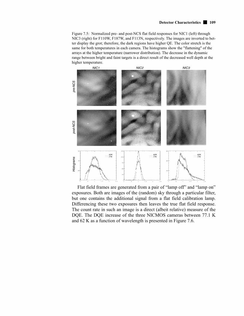
Detector Characteristics 109
Figure 7.5: Normalized pre- and post-NCS flat field responses for NIC1 (left) through NIC3 (right) for F110W, F187W, and F113N, respectively. The images are inverted to bet-ter display the grot; therefore, the dark regions have higher QE. The color stretch is the same for both temperatures in each camera. The histograms show the "flattening" of the arrays at the higher temperature (narrower distribution). The decrease in the dynamic range between bright and faint targets is a direct result of the decreased well depth at the higher temperature.
Flat field frames are generated from a pair of “lamp off” and “lamp on”exposures. Both are images of the (random) sky through a particular filter,but one contains the additional signal from a flat field calibration lamp.Differencing these two exposures then leaves the true flat field response.The count rate in such an image is a direct (albeit relative) measure of theDQE. The DQE increase of the three NICMOS cameras between 77.1 Kand 62 K as a function of wavelength is presented in Figure 7.6.

110 Chapter 7: NICMOS Detectors
Figure 7.6: NICMOS DQE: Comparison between post-SM3B (at operating temperature of 77K) and 1997/1998 (62K) eras.
The average response at 77.1 K increased by about 60% at J, 40% at H,and 20% at K. The resulting wavelength dependence of the absolute DQEfor NICMOS operations under the NCS is shown in Figure 7.7. Here, wehave scaled the pre-launch DQE curve, which was derived from groundtesting of the detectors, to reflect the changes measured at the wavelengthsof the NICMOS filters. These (somewhat indirect) results have beenconfirmed by results from the photometric calibration program which usesobservations of standard stars to measure the absolute DQE of NICMOS.The fine details in these DQE curves should not be interpreted as detectorfeatures, as they may be artifacts introduced by the ground-testing set-up.At the blue end, near 0.9 microns, the DQE at 77.1 K is ~20%; it risesquasi-linearly up to a peak DQE of ~90% at 2.4 microns. At longerwavelengths, it rapidly decreases to zero at 2.6 microns. The NICMOSarrays are blind to longer wavelength emission. When looking at the DQEcurve, the reader should bear in mind that this is not the only criterion to beused in determining sensitivity in the near-IR. For example, thermalemission from the telescope starts to be an issue beyond ~1.7 m. Theshot-noise on this bright background may degrade the signal-to-noiseobtained at long wavelengths, negating the advantage offered by theincreased DQE.
It is important to note, especially for observations of very faint targetsfor which the expected signal-to-noise is low, that the DQE presented hereis only the average for the entire array. Despite the flattening discussedabove, the flat field response is rather non-uniform, and thus the DQEcurves for individual pixels may differ substantially.

Detector Characteristics 111
Figure 7.7: Relative increase of the NICMOS DQE as a function of wavelength for oper-ations at 77.1 K, compared to pre-NCS operations at 62 K.
7.2.4 Read NoiseEach detector has four independent readout amplifiers, each of which
reads a 128 128 quadrant. The four amplifiers of each detector generatevery similar amounts of read noise. This is illustrated in Figure 7.8, whichcompares the pixel read noise distributions for the four quadrants of eachNICMOS camera. The distributions for all quadrants are relatively narrow,with a FWHM of about 8 electrons, indicating that there are only fewanomalously noisy pixels. The read noise is independent of temperature.
For some scientific programs such as ultra-low backgroundobservations (e.g. during the HDF campaigns), read noise can become anon-negligible component of the noise floor. The NICMOS group at STScItherefore has explored a method to lower the read noise in NICMOS databy reducing the digitization noise associated with the conversion fromelectrons to data numbers (DN). This can, in principle, be achieved byusing a different conversion factor (i.e. gain) from e- to DN. Under optimalcircumstances, this can produce a read noise reduction of 10–15%,resulting in exposures that reach up to 0.1 mag deeper. For details, we referto Xu & Boeker (NICMOS ISR-2003-006). However, the use of alternategain settings requires calibration reference files (e.g. flat field or darkexposures) that have been obtained with the same gain. These files will notbe obtained during the NICMOS calibration program. In addition, theCALNICA pipeline is currently not able to process such data correctly.Given the large operational overhead and the rather small scientific benefit,we strongly discourage NICMOS users from requesting non-standard gainsettings. In exceptional circumstances, such requests will be considered on

112 Chapter 7: NICMOS Detectors
a case-by-case basis with the understanding that proper calibration of suchdata is the sole responsibility of the GO.
Figure 7.8: Read noise characteristics of the three NICMOS detectors. Each panel shows the pixel distribution of electronics-induced RMS uncertainties, as measured from a series of difference images of short (0.2s) DARK exposures.
7.2.5 Linearity and SaturationThroughout Cycle 7, the linearity correction of the calibration pipeline
had been based on the assumption that the NICMOS detector response waswell approximated by a linear function until pixel counts reached a certainthreshold. Therefore, no linearity correction was performed below this

Detector Characteristics 113
point. However, the ongoing NICMOS calibration program has shown thatthe detector response is in fact (slightly) non-linear over the full dynamicrange. Figure 7.9 illustrates this behavior.
Figure 7.9: Count rate as a function of total accumulated counts for a typical NICMOS detector pixel. Note that the pixel response is non-linear (i.e., the count rate is not con-stant) over the entire dynamic range.
A revised linearity correction was therefore implemented in theNICMOS calibration pipeline (Cycle 11 and beyond), which corrects dataover the entire dynamic range between zero and the flux level at which theresponse function deviates by more than 5% from the linear approximation.Pixels that reach this threshold during an exposure are flagged as saturated,and are not corrected during the pipeline processing. This saturation pointtypically occurs at about 80% of the well depth.
7.2.6 Count Rate Non-LinearityNICMOS has a significant count rate dependent non-linearity that also
depends on wavelength as described in Section 4.2.4. While we have nophysical explanation for the effect at the time of this writing, we currentlyassume it arises in the detector. Objects fainter than the NICMOS standardstars of about the 12th magnitude will be measured too faint, objects thatare brighter than our standards will seem too bright. The maximum offsetson dark sky backgrounds at F110W are about 0.25 mag in NIC1 and NIC2,and about 0.16 mag in NIC3. Software has been developed to linearize the

114 Chapter 7: NICMOS Detectors
counts in imaging observations. More details on the effect and how tocorrect for it can be found at:
http://www.stsci.edu/hst/nicmos/performance/anomalies/nonlinearity.html.
7.3 Detector Artifacts
7.3.1 ShadingThe NICMOS arrays exhibit a noiseless signal gradient orthogonal to
the direction of primary clocking, which is commonly referred to asshading. It is caused by changes of the pixel bias levels as a function oftemperature and time since the last readout (“delta-time”). The amplitudeof the shading can be as large as several hundred electrons for some pixelsunder some circumstances. The first pixels to be read show the largest biaschanges, with the overall shading pattern decreasing roughly exponentiallywith row number. The shading is a noiseless contribution to the overallsignal, therefore it can be completely removed during pipeline processingonce it has been calibrated with delta-time and temperature.
For a given delta-time (and temperature), the bias level introduced bythe shading remains constant. For MULTIACCUM readout sequences (seeChapter 8) where the time between readouts is increasing logarithmically,the bias level changes with each successive read, and thus the overallshading pattern evolves along the MULTIACCUM sequence. We havecalibrated the dependence of shading as a function of delta-time for each ofthe three NICMOS detectors. This information is used by the calnicapipeline to construct synthetic dark current reference files for NICMOSobservations. The accuracy of this calibration is good (a few percent formost readout times).
The 1999 warm-up monitoring program has shown that the shadingsignal is temperature dependent. Nevertheless, the goodtemperature-stability of the NICMOS/NCS system has enabled accurateshading correction of NICMOS data with a single set of dark currentreference files. Figure 7.10 presents the shading profiles for each camera atthe operating temperature of 77.1 K.
The NICMOS group at STScI will continuously monitor both shadingbehavior and NICMOS temperature stability, and will provide additionalcalibration files should this become necessary.

Detector Artifacts 115
Figure 7.10: Shading profiles for all camera/delta-time combinations measured at 77.1 K (NCS era). The profiles were created by collapsing a dark exposure of the respective inte-gration time along the fast readout direction (after correction for linear dark current and amplifier glow).
NICMOS Shading Profiles
-140
-120
-100
-80
-60
-40
-20
0
NIC
1 D
N
255.999 s127.993 s63.9972 s31.9992 s15.9931 s7.99359 s3.99385 s
1.99398 s
0.997624 s
0.388344 s0.302328 s
0.203000 s
-300
-200
-100
0
NIC
2 D
N
255.999 s
127.993 s
63.9972 s
31.9992 s
15.9931 s
7.99359 s
3.99385 s
1.99398 s
0.997624 s
0.388344 s
0.302328 s
0.203000 s
0 50 100 150 200 250Pixel #
-80
-60
-40
-20
0
NIC
3 D
N
255.999 s
127.993 s
63.9972 s31.9992 s15.9931 s7.99359 s3.99385 s1.99398 s
0.997624 s
0.388344 s0.302328 s
0.203000 s

116 Chapter 7: NICMOS Detectors
7.3.2 Amplifier GlowEach quadrant of a NICMOS detector has its own readout amplifier
situated close to the corners of the detector. Each time the detector is readout, the amplifier warms up and emits infrared radiation that is detected bythe chip. This signal, known as amplifier glow, is largest in the arraycorners with ~80 e-/read, and falls rapidly towards the center of thedetector where it is about 10 e-/read. The signal is cumulative with eachnon-destructive readout of an exposure. It is highly repeatable, and isexactly linearly dependent on number of reads. It also is constant withtemperature, as shown in Figure 7.11.
Figure 7.11: Amplifier glow signal as a function of detector temperature.
In contrast to the shading, the amplifier glow is a photon signal, andthus is subject to Poisson statistics. It therefore contributes to the total noisein NICMOS exposures. Amp-glow images for all three cameras are shownin Figure 7.12. In case of an ACCUM exposure with multiple initial and finalreads (see Chapter 8), the photon noise produced by amplifier glow canoutweigh the read noise reduction from the multiple reads, especially closeto the array corners producing a total noise reduction never larger than ~40–50%. Similarly, the trade-off between improved cosmic ray rejection,reduced read noise, and increased photon noise in a MULTIACCUMsequence is complicated.

Detector Artifacts 117
Figure 7.12: Amplifier glow for Cameras 1 (left) through 3 (right), on a uniform gray-scale, and below a plot of rows (near the bottom) of each camera.
7.3.3 Overexposure of NICMOS DetectorsEffects of photon and cosmic-ray persistence are described in
Section 4.6.
7.3.4 Electronic Bars and BandsElectronic ‘‘bars’’ are an anomaly in NICMOS data taken during Cycles
7 and 7N. They appear as narrow stripes that cross the quadrants of anarray, and occur identically in all 4 quadrants at the same rows/columns ineach. The bars are caused by pick-up of an amplifier signal on one of therow/column address lines, causing a momentary change in the bias for thatpixel.
Similarly, electronic ‘‘bands’’ are caused when one of the NICMOSdetectors is reset while another is being read out. The reset pulse causes asudden jump in the bias of the detector which is being read. The bias jumpthen appears as an imprint on the image that looks like a band.
The bars typically run the length of a quadrant (128 pixels), and are 3pixels wide—the first pixel is lower than the mean, the second is at themean level and the third is higher than the mean, giving the impression ofan undersampled sinusoidal spike with an amplitude of up to ~10 DNpeak-to-peak. If a bar appears in the 0th readout, it will be subtracted fromall the other readouts as part of the normal calibration process, and willappear to be a negative of the above description. The bars run parallel to

118 Chapter 7: NICMOS Detectors
the slow readout direction, which is vertical in NIC1, and horizontal inNIC2 and NIC3. They are almost always broken in at least one place, witha shift of 2–10 pixels in the narrow direction. A more detailed descriptionof the electronic bars and bands is given on the NICMOS WWW site:
http://www.stsci.edu/hst/nicmos.
Since Cycle 11, a modified readout sequence has been implemented forthe three NICMOS cameras which reduces the probability that a detectorwill be reset while another is being read. This procedure is completelytransparent to users and has significantly reduced the electronic bandsproblem.
7.3.5 Detector CosmeticsEach NICMOS detector has a number of pixels that show an anomalous
responsivity. Such “bad pixels” come in various flavors. So-called “hot”pixels have a higher than average dark current, and thus show excessivecharge compared to the surrounding pixels. On the other hand, “coldpixels” are less sensitive to incident photons than the typical pixel. Theanomalously low responsivity of a “cold” pixel could be due to either alower intrinsic DQE of the pixel, or due to grot (see below). Some pixelsdo not even respond at all (“dead pixels”) to incoming light. Quantitativestatistics of the hot/cold and grot pixels in the three NICMOS cameras aregiven in Table 7.1. It is important to note that the impact of bad pixels onthe quality of NICMOS images can be minimized by dithering theobservations.
7.3.6 "Grot"On-orbit flat field exposures taken after the NICMOS installation in
1997 revealed a population of pixels with very low count rates that had notpreviously been seen in ground testing. It is believed that these pixels are atleast partly obscured by debris on the detector surface, most likely smallpaint flakes that were scraped off one of the optical baffles during themechanical deformation of the NICMOS dewar (Sosey, NICMOSISR-99-008 and Boeker et al. 2001 PASP, 113, 859). Additional grot hascollected on the detectors since its revival. NIC1 appears to be the mostaffected with an additional chunk of grot in the lower right quadrant. Thisso-called “grot” affects approximately 100–200 pixels in each NICMOScamera. The largest pieces of grot in NIC1 are shown in Figure 7.13.Again, dithering is recommended to minimize the impact of grot.

Detector Artifacts 119
Figure 7.13: A NIC1 flat field image shows the largest of the groups of pixels affected by debris (“grot”). These bits of “grot” are roughly 5 by 9 pixels (upper left) and 5 by 6 pixels (lower right).

CHAPTER 8:
Detector Readout ModesIn this chapter . . .
8.1 Introduction
NICMOS has four detector readout modes that may be used to take data.After the observing time has been approved, the readout mode will beselected by the observer when completing the Phase II proposal entry.However, potential observers may want to understand the characteristics ofthe NICMOS readout modes to help design their Phase I proposal.
There are three supported readout modes:
1. Multiple-accumulate Mode (MULTIACCUM).
2. Accumulate Mode (ACCUM).
3. Acquisition Mode (ACQ).
The ACCUM mode is, however, supported only for NREAD=1. Forother configurations the ACCUM mode is available but not supported, i.e.the observer must request the use through a Contact Scientist during
8.1 Introduction / 1218.2 Multiple-Accumulate Mode / 123
8.3 MULTIACCUM Predefined Sample Sequences (SAMP-SEQ) / 125
8.4 Accumulate Mode / 128
8.5 Read Times and Dark Current Calibration in ACCUM Mode / 130
8.6 Trade-offs Between MULTIACCUM and ACCUM / 131
8.7 Acquisition Mode / 132
Nearly all observers should use the MULTIACCUM mode, as it providesthe highest quality scientific data.
121

122 Chapter 8: Detector Readout Modes
preparation of the Phase II proposal. The basic scientific rationale behindeach of these modes, and a summary of their capabilities is outlined inTable 8.1, along with a recommendation regarding their use. The Phase IIproposal instructions needed to identify the readout modes are given inparentheses under the mode name.
Table 8.1: Readout Modes and their Functions.
Mode Use Functionality Recommendation
Multiple-Accumulate(MULTIACCUM)
Faint targets.Large dynamic range.Optimal image construction.Ground processing of cosmic rays and saturation.
Multiple non-destructive read-outs at specific times duringan integration.0.215 < t < 8590 seconds.Number of readouts 25.
Recommended for most programs.Ensures the highest dynamic range. Most effective for cor-rection of cosmic ray hits and saturation.
Accumulate (ACCUM)
Simplest observing mode. Produces a single image.
t > 0.57 seconds. MULTIACCUM is rec-ommended instead of ACCUM for almost all programs; ACCUM might be useful with large numbers of very short exposures (see Section 8.6).
Onboard Acquisition(ACQ)
For coronagraphy only.Locate brightest source in a subar-ray and reposition telescope to place source in coronagraphic hole.
ACCUM exposures are obtained, combined with cosmic ray rejec-tion, hole located, sources located and centered.
Reasonably bright sources in uncrowded fields. See Chapter 5 for more details.
Bright Object(BRIGHTOBJ)
For coronagraphic acquisition of bright targets which would saturate the arrays in the other modes with the shortest integration time allowed.
reset/read/wait/read each pixel sequentially in a quadrant.0.001024 < t < 0.2 seconds.
When possible use a narrow filter with MULTIACCUM instead.
The BRIGHTOBJ mode is not supported for Cycle 13 and later cycles;it is, however, an available mode for the special case of acquisition ofvery bright targets under the coronagraphic hole. See Appendix C fora more detailed description of this mode.

Multiple-Accumulate Mode 123
Detector Resetting as a ShutterNICMOS does not have a physical shutter mechanism. Instead, the
following sequence of operations are performed to obtain an exposure:
• Array reset: All pixels are set to zero—the bias level.
• Array read: The charge in each pixel is measured and stored in the on-board computer’s memory. This happens as soon as practical after the array reset. In effect, a very short exposure image is stored in memory.
• Integration: NICMOS exposes for the period specified for the inte-gration.
• Array read: The charge in each pixel is measured and stored in the on-board computer’s memory.
8.2 Multiple-Accumulate Mode
One of the concepts inherent in the operation of the NICMOS arrays istheir non-destructive readout capability.
During the exposure, all pixels are first reset via three separate passesthrough the detector. The reset is immediately followed by a fourth passthrough the detector, which non-destructively reads and stores the pixelvalues. This marks the beginning of the integration. The first array readwill then be followed by one or more non-destructive readings of thedetector. The last non-destructive readout marks the end of the integration.The total integration time is given by the difference in time between thefirst and the last array read.
The non-destructive nature of the NICMOS readout offers elaboratemethods of using the instrument, which aim at optimizing the scientificcontent of the results. In particular, it is possible to read-out images atintermediate stages of an integration and return both these and the finalimage to the ground. This mode of operation is known asMultiple-Accumulate (MULTIACCUM). The observer uses this capabilityby specifying one of the pre-defined MULTIACCUM sequences,SAMP-SEQ (see next section) and the number of samples NSAMP thatcorresponds to the desired integration time. The list of supportedMULTIACCUM sequences is given in the next section. These sequences areeither linearly spaced or logarithmically spaced. Linearly spaced exposuresmay be useful for faint targets where cosmic ray filtering is important whilelogarithmically spaced exposures permit the observation of a widedynamic range. The process is shown schematically in Figure 8.1 for thecase of logarithmically spaced intervals with NSAMP=4.

124 Chapter 8: Detector Readout Modes
In MULTIACCUM the detector reset is followed by a single read of theinitial pixel values (zeroth read). Then a sequence of non-destructive arrayreadouts are obtained at times specified by the selected sequence. Up to 25readouts can be specified spanning a total integration time from 0.203seconds to 8590.0 seconds. The last read of the detector array ends theexposure and thus the last NSAMP will be selected to give the totalexposure time. All of the readouts, including the initial readout, are storedand downlinked without any onboard processing. For N readouts, thismode requires the storage and transmission (downlink) of N+1 times asmuch data volume as for ACCUM mode. (See Section 8.6 for trade-offsbetween MULTIACCUM and ACCUM readout modes.)
In most cases, MULTIACCUM mode provides the highest qualityscientific data. The benefits of obtaining observations in MULTIACCUMmode fall into two areas.
• The dynamic range of the observation is greatly increased. Rather than being limited by the charge capacity of a NICMOS pixel (a few 105 electrons), an observation’s dynamic range is in principle lim-ited by the product of the pixel capacity and the ratio of the longest and shortest exposures (8590.0 and 0.203 seconds).
• An image can be reconstructed by processing the stack of readouts to cope with the effects of cosmic rays and saturation.
MULTIACCUM provides the best choice for deep integrations orintegrations on fields with objects of quite different brightness.
MOST observers should use MULTIACCUM for their observations.Starting with Cycle 14, the four MIF MULTIACCUM timingsequences (MIF512, MIF1024, MIF2048, and MIF3072) have beenreplaced with four new SPARS timing sequences (SPARS4, SPARS16,SPARS32, and SPARS128). The new SPARS sequences can be mostuseful for fields with faint sources; i.e. nebulae, star clusters and gal-axies.

MULTIACCUM Predefined Sample Sequences (SAMP-SEQ) 125
Figure 8.1: Example MULTIACCUM with NSAMP = 4.
8.3 MULTIACCUM Predefined Sample Sequences(SAMP-SEQ)
For the user’s convenience, and to minimize the volume of commandinginformation to be sent to HST, a set of sequences has been defined whichshould cover nearly all applications of MULTIACCUM. These are listed inTable 8.2. The observer specifies the name of the sequence and the numberof samples to be obtained. The SCAMRR and MCAMRR are to be used whenthe fastest temporal sampling is desired. The SPARS4, SPARS16,SPARS32, SPARS64, SPARS128 and SPARS256 sequences haverelatively few readouts and may be helpful when two or more cameras areoperated in parallel (in particular they generally permit a second and thirdcamera to operate in parallel with a minimal impact on the operation of theprimary camera). SPARSXX is also recommended for observations offields where only faint targets are present. The STEPXX sequences all startwith three rapid readouts and then are logarithmically spaced to provide alarge dynamic range up to their defined time (e.g., STEP64 has log stepsup to 64 seconds) and then revert to linear spacing. The STEPXXsequences are recommended for observations involving both bright andfaint targets, where high dynamic range is required.
ONBOARD
TO GROUND
Flu
sh
Non-destructivereadouts0th 1st 2nd 3rd 4th
Pix
el v
alue
s re
set
samptime01 = Time interval since the START of the 0th readout
samptime02 = Time interval since the START of the 0th readout
samptime03 = Time interval since the START of the 0th readout
}5 RAW imagesreturned
# images = nsamp + 1
samptime04 = total integration timeTime interval since the start ofthe 0th readout

126 Chapter 8: Detector Readout Modes
The fastest time to read a single camera is 0.203 seconds, while 0.303seconds is the fastest time when more than one camera is used.Accordingly, the MULTIACCUM sequences have been set up so that thefirst read is always the fastest time possible. The second read for all of thesequences, except for the SCAMRR, has a time of 0.606 seconds.
Table 8.2: MULTIACCUM SAMP-SEQs.
Sequence Name
Readout Times Description
SCAMRR 0.2031.2182.2333.2484.263
0.4061.4212.4363.4514.466
0.6091.6242.6393.6544.669
0.8121.8272.8423.8574.872
1.0152.0303.0454.0605.075
Single camera fastest possible operation.
MCAMRR 0.3031.8183.3334.8486.363
0.6062.1213.6365.1516.666
0.9092.4243.9395.4546.969
1.2122.7274.2425.7577.272
1.5153.0304.5456.0607.575
Fastest possible operation with 2 or 3 cameras used in parallel.
STEP1 0.3033.9898.97913.96918.959
0.6064.9879.97714.96719.957
0.9955.98510.97515.96520.955
1.9936.98311.97316.96321.953
2.9917.98112.97117.96122.951
Rapid reads up to 1 second then 1 second steps.
STEP2 0.3035.98115.95125.92135.891
0.6067.97517.94527.91537.885
0.9959.96919.93929.90939.879
1.99311.96321.93331.90341.873
3.98713.95723.92733.89743.867
Rapid reads up to 2 seconds then 2 second steps.
STEP8 0.3037.98147.95187.921127.891
0.60615.97555.94595.915135.885
0.99523.96963.939103.909143.879
1.99331.96371.933111.903151.873
3.98739.95779.927119.897159.867
Rapid reads up to 8 seconds then 8 second steps.
STEP16 0.3037.98179.951159.921239.891
0.60615.97595.945175.915255.885
0.99531.969111.939191.909271.879
1.99347.963127.933207.903287.873
3.98763.957143.927223.897303.867
Rapid reads up to 16 seconds then 16 second steps.
STEP32 0.3037.981127.969287.969447.969
0.60615.975159.969319.969479.969
0.99531.969191.969351.969511.969
1.99363.969223.969383.969543.969
3.98795.969255.969415.969575.969
Rapid reads up to 32 seconds then 32 second steps.
STEP64 0.3037.981191.965511.955831.945
0.60615.975255.963575.953895.943
0.99531.969319.961639.951959.941
1.99363.969383.959703.9491023.939
3.987127.967447.957767.9471087.937
Rapid reads up to 64 seconds then 64 second steps.

MULTIACCUM Predefined Sample Sequences (SAMP-SEQ) 127
STEP128 0.3037.981255.961895.9311535.901
0.60615.975383.9551023.9251663.895
0.99531.969511.9491151.9191791.889
1.99363.969639.9431279.9131919.883
3.987127.967767.9371407.9072047.877
Rapid reads up to 128 sec-onds then 128 second steps.
STEP256 0.3037.981255.9611535.9612815.961
0.60615.975511.9611791.9613071.961
0.99531.969767.9612047.9613327.961
1.99363.9691023.9612303.9613583.961
3.987127.9671279.9612559.9613839.961
Rapid reads up to 256 sec-onds then 256 second steps.
SPARS4 0.30316.00436.01456.02476.034
0.60620.00640.01660.02680.036
3.99824.00844.01864.02884.038
8.00028.01048.02068.03088.040
12.00232.01252.02272.03292.042
Two rapid readouts then 4 second steps.
SPARS16 0.30364.000144.005224.010304.015
0.60680.001160.006240.011320.016
15.99796.002176.007256.012336.017
31.998112.003192.008272.013352.018
47.999128.004208.009288.014368.019
Similar to STEP16 but with-out the rapid initial readouts.
SPARS32 0.303128.004288.004448.004608.004
0.606160.004320.004480.004640.004
32.004192.004352.004512.004672.004
64.004224.004384.004544.004704.004
96.004256.004416.004576.004736.004
Similar to STEP32 but with-out the rapid initial readouts.
SPARS64 0.303255.988575.978895.9681215.958
0.606319.986639.976959.9661279.956
63.994383.984703.9741023.9641343.954
127.992447.982767.9721087.9621407.952
191.990511.980831.9701151.9601471.950
Similar to STEP64 but with-out the rapid initial readouts.
SPARS128 0.303512.0001152.0051792.0102432.015
0.606640.0011280.0061920.0112560.015
127.997768.0021408.0072048.0122688.017
255.998896.0031536.0082176.0132816.018
383.9901024.0041664.0092304.0142944.019
Similar to STEP128 but without the rapid initial read-outs.
SPARS256 0.3031023.9962303.9963583.9964863.996
0.6061279.9962559.9963839.9965119.996
255.9961535.9962815.9964095.9965375.996
511.9961791.9963071.9964351.9965631.996
767.9962047.9963327.9964607.9965887.996
Similar to STEP256 but without the rapid initial read-outs.
Table 8.2: MULTIACCUM SAMP-SEQs.
Sequence Name
Readout Times Description

128 Chapter 8: Detector Readout Modes
8.4 Accumulate Mode
The Accumulate Readout Mode (ACCUM) generates the simplest basicexposure. In its simplest incarnation, two array readouts, illustrated inFigure 8.2, it is analogous to a WFPC2 or ACS readout. Its main differencerelative to a MULTIACCUM exposure with NSAMP=2 (or two readoutsselected) is that the first array read gets subtracted from the second arrayread by the on-board computer, and only the difference image is sent to theground. In other words, the returned image is the difference between thesecond and the first pass pixel values, and the integration time is defined asthe time between the first and second read of the first pixel. The minimumexposure time is ~0.6 sec, and the minimum time between successiveexposures is ~8–12 seconds. ACCUM does not allow pipeline identificationof cosmic ray events or to correct for pixel saturation.
Figure 8.2: Basic NICMOS Readout—Simple Two-Sample Readout.
Multiple Initial and Final Sample ReadoutIn ACCUM mode multiple initial and final reads can be obtained in place
of the single initial and final readouts. In this case, after the detector arrayis reset, it will be followed by 1–25 (specified by the NREAD parameter)reads of the initial pixel values which are averaged onboard to define the
ONBOARD
TO GROUND
Initial readout Final readoutof pixel values of pixel values
Difference = Final - Initial Readouts
Integration Time = Read time of 1st pixel of 1st readout - Read time of 1st pixel of final readout
Pix
el v
alue
s re
set
Flu
sh Non-destructivereadouts
Flush time is 0.615s and is followed immediately by the Initial Readout.

Accumulate Mode 129
initial signal level. After the exposure time has elapsed, the final pixelvalues are again read NREAD times and averaged onboard. The datadownlinked is the difference between the initial and final average signallevels for each pixel. The integration time is defined as the time betweenthe first read of the first pixel in the initial NREAD passes and the first readof the first pixel in the final NREAD passes. The use of multiple reads inACCUM mode is illustrated in Figure 8.3 for the case of NREAD = 4.
The advantage of this method is a reduction in the read noise associatedwith the initial and final reads. In theory the read noise should be reducedby 1/(n)1/2 where n is the number of reads. However, the amplifier glow(see Chapter 7) adds extra signal and associated photon noise for each read,especially towards the corners of the array. Amplifier glow is an additivenoise source large enough that for NREAD > 9 there is little further gain innoise. In practice, the maximum improvement in effective read noise over asingle initial and final read is no larger than a factor 40–50%, due to theadded amplifier glow that each read-out adds to the final noise budget. Forintegrations where source photon noise or dark current noise exceeds thedetector read noise, the multiple readouts may not offer much advantage.This option puts a higher burden on the CPU and requires an additionaltime per readout of 0.6 seconds. This mode does not allow pipelineidentification of cosmic ray events or correction for pixel saturation.
Starting from Cycle 12, ACCUM is available but unsupported for allmodes with NREAD > 1. This means that the mode should only beused if dictated by special observing requirements.

130 Chapter 8: Detector Readout Modes
Figure 8.3: ACCUM Mode with Four Initial and Final Readouts.
8.5 Read Times and Dark Current Calibration in ACCUM Mode
Because of the effects of shading, and the possibility that the underlyingdark current may vary with time since reset, the removal of dark current(for calibration purposes, we implicitly assume shading and amplifier glowis a part of the time variable “dark current”) from NICMOS data is morecomplicated than for other instruments. The most accurate way to removethe dark current from any observation is a measurement of the dark currentwith an identical integration time and at the same detector temperature. ForACCUM observations we encourage observers to select exposure times thatcorrespond to existing delta-times of the pre-defined MULTIACCUM
ONBOARD
TO GROUND
Flu
sh first 4 (=nreads), xi last 4 (=nreads), yi
Integration Time = Read time of 1st pixel of 1st Final Readout - Read time of 1st pixel of 1st Initial Readout
Pix
el v
alue
s re
set
Non-destructivereadouts
} }
xi yi
yi xi–
4------------------------------
}}

Trade-offs Between MULTIACCUM and ACCUM 131
sequences (Table 8.2). These available delta-times are also listed in Table8.3 below.
Table 8.3: Recommended Exposure Times with Dark Current Calibration.
STScI is not planning to obtain dedicated ACCUM dark observations, butdark reference files for ACCUM observations can be constructed fromMULTIACCUM darks with identical delta-times.
8.6 Trade-offs Between MULTIACCUM and ACCUM
There are a variety of advantages to the MULTIACCUM mode. First, theability present in a MULTIACCUM exposure to filter out CR hits whichoccur during the exposure is lost in the ACCUM mode. We find forNICMOS that typically between 2 and 4 pixels are hit per second percamera by CRs: most of these are low energy and so can be filtered out of aMULTIACCUM exposure by the calibration pipeline software. In ACCUMmode, the process of CR removal requires separate exposures and has to bedone in post-processing. Second, the ability to detect pixel saturation,which again is done automatically for MULTIACCUM observations by thecalibration software, can in some circumstances be lost in ACCUM mode.
Time (seconds) (NREAD=1)
0.203
0.303
0.389
0.998
1.994
3.994
7.994
15.994
32.000
63.998
127.994
256.000
383.999
511.998
132 Chapter 8: Detector Readout Modes
This is because the time elapsed between the first read for each pixel andthe reset immediately prior to the read is approximately 0.2 seconds.During this time, pixels exposed to a bright target will accumulatesignificant signal, which is then present in the first read. When this issubtracted on-board in ACCUM mode, all the charge accumulated in thetime between reset and read will be subtracted. If the pixel has saturatedduring the exposure, the difference between initial and final reads will beless than the expected saturation value for the pixel, and thus it may beimpossible to recognize that the pixel is saturated. Therefore, in the case ofbright targets, erroneous signal levels may be recorded in ACCUM mode.Third, in ACCUM mode, even if pixel saturation is detected, it is notpossible to repair the data obtained in the saturated pixel. In MULTIACCUMmode, pixels which have saturated can be repaired by using the results ofprevious, unsaturated reads during the same exposure.
Given that there is so much more information present in aMULTIACCUM dataset than in an ACCUM dataset, it may seem obvious thatMULTIACCUM should always be the preferred readout mode. In practice,there can be trade-off in a few specific cases.
Because of the fixed read-out patterns available for use inMULTIACCUM mode (the SAMP-SEQs), in order to make an exposure oftotal integration time a minute or two, it is necessary in most modes toperform a significant number of readouts. This may lead to a significantvolume of data to process. Additionally, the readouts are initially stored ina buffer in the NICMOS flight computer. A maximum of 94 readouts canbe stored in this buffer, after which the content of the buffer must bedumped to the Solid State Recorder. A full dump of 94 reads takes aboutthree minutes. The data dumps occur in parallel with the beginning ofanother set of exposures (and thus do not ‘penalize’ the available observingtime) in the vast majority of, but not all, circumstances. Thus, during thepreparation of the Phase II proposals, some observers with very short (1-2minutes) exposures may consider the trade-offs between ACCUM andMULTIACCUM.
In conclusion, in cases where a multitude of short duration exposuresmust be made per orbit, and data volume could be a problem, ACCUM maypossibly (but not necessarily) be a good choice. In all other cases it is likelythat MULTIACCUM will yield the best results, and therefore, werecommend that all observers attempt to use MULTIACCUM.
8.7 Acquisition Mode
Images obtained using the coronagraph in Camera 2 may be taken usingany of the detector read-out modes. An ACQ mode observation performs anautonomous on-board acquisition (Mode-2 Acquisition) for subsequentcoronagraph images. This mode is described in detail in Chapter 5(Coronagraphy).

CHAPTER 9:
Exposure TimeCalculations
In this chapter . . .
9.1 Overview: Web based NICMOS ETC
In this section we describe some instrument-specific behavior whichmust be taken into account when estimating required exposure times. TheWWW NICMOS Exposure Time Calculator (ETC) provides the mostconvenient means of estimating count rates and signal-to-noise ratios(SNRs) for imaging observations. The ETC handles either point sources orextended objects and can be accessed from:http://www.stsci.edu/hst/nicmos/tools/New_APT_ETC
Two NICMOS ETCs are available to observers, an imaging ETC and aSpectroscopic ETC for grism users. Previously, only the imaging ETC wasavailable. The Spectroscopic ETC was delivered on November 8, 2004along with an updated imaging ETC.
The imaging NICMOS WWW ETC is documented in an InstrumentScience Report (Arribas, NICMOS ISR-2004-002). Recent updates arealso explained in its help file (accessible from the user interface). The ETCgenerates either the exposure time required for a specified SNR or theexpected SNR for a user-defined exposure time. It will also indicate the
9.1 Overview: Web based NICMOS ETC / 1339.2 Calculating NICMOS Imaging Sensitivities / 136
133

134 Chapter 9: Exposure Time Calculations
read noise and the source and background count rate, as well as thesaturation-limited exposure time for the object in question.
A few comments about the limitations of making exposure time andSNR estimates are in order here.
NICMOS performance with the NCS has changed (relative to Cycles 7and 7N) because the instrument now operates at a different temperature.This has improved the Detector Quantum Efficiency (DQE), but has alsoincreased the dark current. The ETC has been updated to use parametersfor Cycle 11 and beyond, with a temperature of 77.15K.
The instrumental characteristics used by the ETC are average valuesacross the field of view of the camera. The actual sensitivity will varyacross the field because of DQE variations (see Chapter 7 for details). Asecond source of spatial variation not included in the ETC occurs near thecorners of the chip because of amplifier glow (see Section 7.3.2).
For photon-limited observations (limited either by the target count rateor the background), SNR increases as the square root of the totalobservation time, regardless of how the observation is subdivided intoindividual exposures. However, some NICMOS observations may besignificantly affected by read noise, and the net SNR from the sum ofseveral exposures will depend on the relative contributions of read noiseand photon noise. Read noise variations that depend on different readsequences are not accounted for in the ETC.
Phenomena such as cosmic ray persistence (Chapter 4) can degradesensitivity for faint object imaging by increasing the level of backgroundnoise. The impact of cosmic ray persistence is not easily quantified becauseit is non-Gaussian, correlated noise. It is not possible to predict the extentof this effect at the time the observations are planned, so it is not includedin the ETC calculations. Additional information on the ETC and itsstructure can be found in the Instrument Science Reports (ISRs) posted onthe STScI NICMOS Instrument Web page.
http://www.stsci.edu/hst/nicmos/
The WWW NICMOS Exposure Time Calculator (ETC) should beregarded as the tool of choice for estimating integration times for NIC-MOS observations. The ETC provides the most accurate estimates withthe most current information on instrument performance; its referencetables are constantly updated with the most recent values of the instru-ment’s characteristics as our knowledge of the NICMOS performanceunder NCS operations improves. Please check the NICMOS Web sitefor recent ETC updates.

Overview: Web based NICMOS ETC 135
The ETC does not take the count rate non-linearity (Section 4.2.4) intoaccount. This is especially relevant for faint and/or low surface brightnessobservations on a low background at wavelengths shorter than 1.6 microns.The effect depends on the count rate in each individual pixel and istherefore hard to model in the ETC. To correct for this non-linearity, forfaint objects (mAB > ~20) one should use a 0.25 mag fainter object in theETC for F110W in NIC1 and NIC2, and 0.16 mag fainter for NIC3, whenone has an average background. The effect is always less at longerwavelengths and brighter backgrounds.
9.1.1 Instrumental Factors
DetectorsThe detector properties which will affect the sensitivity are simply those
familiar to ground-based optical and IR observers, namely dark current andread noise, and the detector quantum efficiency (DQE). The dark currentand DQEs measured in Cycle 11 are included in this ETC (see Chapter 7for more details). The variation of the DQE as a function of wavelengthand temperature is also taken into account. The ETC currently does nottake the count rate non-linearity described in Section 4.2.4 into account.Faint objects may be affected by as much as 0.25 mag in NIC1 and NIC2,and 0.16 mag in NIC3 at the shorter wavelengths.
OpticsNICMOS contains a fairly small number of elements which affect the
sensitivity. These elements are the filter transmission, the pixel field ofview (determined by the NICMOS optics external to the dewar, incombination with the HST mirrors), the reflectivities and emissivities ofthe various mirrors and the transmission of the dewar window.
Filter transmissions as a function of wavelength were measured in thelaboratory and convolved with OTA, NICMOS fore-optics and detectorresponse. The resulting curves are presented in Appendix A.
NICMOS contains a total of seven mirrors external to the dewar, each ofwhich reduces the signal received at the detector. The mirrors are silvercoated (except for the field divider assembly which is gold coated) for areflectivity of 98.5%. The dewar window has a transmission of roughly93%. Therefore, the combination of optical elements is expected totransmit ~84% of the incoming signal from the OTA.
The sensitivity will obviously be affected by the pixel field of view. Thesmaller the angular size of a pixel, the smaller the fraction of a given sourcethat will illuminate the pixel, but compensating will be a lower skybackground. Finally, the optical efficiency will be degraded further by thereflectivities of the aluminum with MgF2 overcoated HST primary andsecondary mirrors.

136 Chapter 9: Exposure Time Calculations
Background RadiationAt long wavelengths (> 1.7 microns) the dominant effect limiting the
NICMOS sensitivity is the thermal background emission from thetelescope. The magnitude of this background mainly depends on thetemperatures of the primary and secondary mirrors and their emissivities.At shorter NICMOS wavelengths, sensitivities are affected by the zodiacalbackground. Both sources of background are described in Chapter 4.
9.2 Calculating NICMOS Imaging Sensitivities
In some situations it may be desirable to go through each step of thecalculation. To facilitate calculations when the Web connection is notpossible, in this section we provide recipes for determining thesignal-to-noise ratio or exposure time by hand. These calculations refer tothe brightest pixel (i.e., aperture of 11 pixel). These calculations do nottake the count rate non-linearity into account described in Section 4.2.4.
9.2.1 Calculation of Signal-to-Noise RatioThe first step in this process is to calculate the electrons/second/pixel
generated by the source. For this we need to know the flux in the centralpixel Fj in Jansky/pixel. Please refer to Appendix A to calculate the fractionof flux that will lie in the central pixel for any camera/filter combination,and Appendix B for unit conversions.
Then the electron count in that pixel due to the continuum source is
where:
is the transmittance of the entire optical train up to the detector, excluding the filters;
is the detector quantum efficiency; is the filter transmittance; is the unobscured area of the primary;
E is a constant given by:
where h is Planck’s constant and the wavelength. The quantities Fj, opt,det and filt are all frequency dependent. The expression for Cc has to beintegrated over the bandpass of the filter, since some of the terms varysignificantly with wavelength. It should be noted that to determine Cc moreaccurately, the source flux Fj should be included in the integral over thefilter bandpass, since the source flux is bound to be a function ofwavelength.
Cc FjoptdetfiltAprimE Fjc e-/sec/pixel ==
opt
det
fillt
Aprim
E 1026–
h =

Calculating NICMOS Imaging Sensitivities 137
For an emission line with intensity Ilj (in W m-2 pixel-1) falling in thebandpass of the filter, the counts in e-/s are given by:
where E is defined as before. In this case, the detector quantum efficiencyand filter transmission are determined for the wavelength of the emissionline. The total signal per pixel is the sum of the continuum and line signalscalculated above, namely Cs=Cc+Cl.
The source signal is superimposed on sky background and thermalbackground from warm optics. At > 1.7 m the background is oftenmuch brighter than the source. In such cases the observation is backgroundlimited, not read noise limited. There is little point in increasing thenumber of multiple initial and final reads when the observation isbackground-limited, though multiple exposures and dithering will helpcosmic ray removal and correction of other effects such as persistence frompreviously-observed bright objects.
The other components of unwanted signal are read noise, Nr, and darkcurrent, Id (in e-/s/pixel). By read noise, we mean the electronic noise in thepixel signal after subtraction of two reads (double correlated sampling).
It is now possible to calculate the signal-to-noise ratio expected for anexposure of duration t seconds:
where Cs, the count rate in e-/sec/pixel, is the sum of Cc plus Cline, B is thebackground in e-/sec/pixel (also listed in Tables 9.1, 9.2, and 9.3), Id is thedark current in e-/sec/pixel and Nr is the read-out noise, in e-/pixel, for oneinitial and one final read. Although the effective Nr can vary somewhatdepending on the readout sequence, ETC considers a fixed value percamera of about 26 e-.
It is important to note that in these equations, the flux to be entered(either Fj or Ilj or both) is not the total source flux, but the flux falling on apixel. In the case of an extended source this can easily be worked out fromthe surface brightness and the size of the pixel. For a point source, it will benecessary to determine the fraction of the total flux which is containedwithin the area of one pixel and scale the source flux by this fraction. ForCamera 1 in particular, this fraction may be quite small, and so will make asubstantial difference to the outcome of the calculation. Appendix A givesthe fraction of the PSF falling in the brightest pixel assuming a point sourcecentered on the pixel, for each filter.
The signal-to-noise ratio evaluated by a fit over the full PSF for pointsources would, of course, be larger than this central pixel SNR; thisdiscrepancy will be largest for the higher resolution cameras and for thelongest wavelengths.
Cl Iljoptdet filt AprimE Iij e-/sec/pixel ==
SNRCst
Cs B Id+ + t Nr2
+--------------------------------------------------=

138 Chapter 9: Exposure Time Calculations
The average values for c and for each filter are denoted as and andare listed in Tables 9.1, 9.2, and 9.3 for a detector temperature of 77.1K. (Note that the above tables are not necessarily updated and the results inS/N could be off by ~20% (or more) in some cases. The Web based ETC,which is updated and provides more accurate results, should be used forany serious ETC calculation.) For estimating we have assumed a sourcewith an effective temperature of 5,000K, but the Web based ETC will takethe spectral type chosen by the user to integrate over the bandpass. Foremission lines in the wings of the filter bandpass, another correction factormay be needed which can be estimated from filter transmission curves inAppendix A.
9.2.2 Saturation and Detector LimitationsGiven a particular filter-detector combination and a requested target
flux, there is an exposure time above which the detector starts to saturate.The WWW NICMOS ETC will produce this exposure time when itperforms the requested estimation.
9.2.3 Exposure Time CalculationThe other situation frequently encountered is when the required
signal-to-noise is known, and it is necessary to calculate from this theexposure time needed. In this case one uses the same instrumental andtelescope parameters as described above, and the required time is given by:
c
c
tSNR 2 Cs B Id+ + SNR 4 Cs B Id+ + 2
4 SNR 2Cs2Nr
2++
2Cs2
------------------------------------------------------------------------------------------------------------------------------------------------------------=

Calculating NICMOS Imaging Sensitivities 139
Table 9.1: NIC1 Filter Sensitivity Parameters (per pixel).
FilterT= 77.15K
c [e-/sec/Jy] [e- /sec/(W/m2)] B [e-/sec]
F090M 0.765E+06 0.161E+19 0.115E-01
F095N 0.433E+05 0.110E+19 0.104E-02
F097N 0.522E+05 0.137E+19 0.104E-02
F108N 0.605E+05 0.199E+19 0.104E-02
F110M 0.135E+07 0.302E+19 0.188E-01
F110W 0.385E+07 0.415E+19 0.532E-01
F113N 0.729E+05 0.231E+19 0.104E-02
F140W 0.608E+07 0.944E+19 0.100E+00
F145M 0.153E+07 0.624E+19 0.170E-01
F160W 0.337E+07 0.948E+19 0.635E-01
F164N 0.149E+06 0.697E+19 0.277E-02
F165M 0.168E+07 0.898E+19 0.284E-01
F166N 0.146E+06 0.691E+19 0.190E-02
F170M 0.176E+07 0.953E+19 0.478E-01
F187N 0.157E+06 0.907E+19 0.213E-01
F190N 0.157E+06 0.951E+19 0.282E-01
POL0S 0.126E+07 0.136E+19 0.177E-01

140 Chapter 9: Exposure Time Calculations
Table 9.2: NIC2 Filter Sensitivity Parameters (per pixel).
FilterT=77.15K
c [e-/sec/Jy] [e-/sec/(W/m2)] B [e-/sec]
F110W 0.443E+07 0.458E+19 0.185E+00
F160W 0.371E+07 0.104E+20 0.170E+00
F165M 0.187E+07 0.996E+19 0.818E-01
F171M 0.723E+06 0.930E+19 0.421E-01
F180M 0.693E+06 0.997E+19 0.774E-01
F187N 0.177E+06 0.102E+20 0.446E-01
F187W 0.198E+07 0.105E+20 0.645E+00
F190N 0.172E+06 0.106E+20 0.578E-01
F204M 0.956E+06 0.134E+20 0.153E+01
F205W 0.572E+07 0.199E+20 0.351E+02
F207M 0.127E+07 0.124E+20 0.345E+01
F212N 0.192E+06 0.125E+20 0.697E+00
F215N 0.176E+06 0.123E+21 0.831E+00
F216N 0.190E+06 0.130E+20 0.104E+01
F222M 0.131E+07 0.139E+20 0.130E+02
F237M 0.148E+07 0.195E+20 0.506E+02
POL0L 0.943E+06 0.757E+19 0.120E+01

Calculating NICMOS Imaging Sensitivities 141
Table 9.3: NIC3 Filter Sensitivity Parameters (per pixel).
FilterT= 77.15K
c [e-/sec/Jy] [e- /sec/(W/m2)] B [e-/sec]
F108N 0.657E+05 0.214E+19 0.188E-01
F110W 0.399E+07 0.419E+19 0.119E+01
F113N 0.794E+05 0.242E+19 0.208E-01
F150W 0.673E+07 0.104E+20 0.276E+01
F160W 0.356E+07 0.101E+20 0.104E+01
F164N 0.157E+06 0.747E+19 0.453E-01
F166N 0.151E+06 0.736E+19 0.400E-01
F175W 0.916E+07 0.189E+20 0.108E+03
F187N 0.164E+06 0.940E+19 0.207E+00
F190N 0.172E+06 0.105E+20 0.282E+00
F196N 0.181E+06 0.109E+20 0.613E+00
F200N 0.186E+06 0.111E+20 0.898E+01
F212N 0.184E+06 0.123E+20 0.322E+01
F215N 0.169E+06 0.117E+20 0.384E+01
F222M 0.126E+07 0.136E+20 0.606E+02
F240M 0.182E+07 0.185E+20 0.382E+03

CHAPTER 10:
Overheads andOrbit Time
DeterminationIn this chapter . . .
10.1 Overview
Once the set of science exposures and any additional target acquisitionor calibration exposures required for the science program have beendetermined, they must be converted into a total number of orbits.Generally, this is a straightforward exercise involving tallying up theoverheads on the individual exposures and on the selected pattern (seeAppendix D), packing the exposure and overhead times into individualorbits, and tallying up the results to determine the total orbit request. Thisprocess may need to be iterated, in order to seek the most efficient use ofthe orbit time.
For information on the observatory policies and practices with respect toorbit determination, please refer to the Call for Proposals/Phase I ProposalInstructions at:
http://www.stsci.edu/hst/HST_overview/documents.
Below, we provide a summary of the NICMOS specific overheads, andgive an example to illustrate how to calculate orbit requirements for PhaseI Proposals.
10.1 Overview / 14310.2 NICMOS Exposure Overheads / 144
10.3 Orbit Use Determination / 147
143

144 Chapter 10: Overheads and Orbit Time Determination
10.2 NICMOS Exposure Overheads
The overheads on exposures are summarized in Table 10.1. All numbersare approximate and, for the observatory level overheads, rounded up tothe nearest half minute. These overhead times are to be used (inconjunction with the actual exposure time and the Phase I ProposalInstructions) to estimate the total time in orbits for NICMOS proposal timerequests. After an HST proposal is accepted, the observer will be asked tosubmit a Phase II proposal to allow scheduling of the approvedobservations. At that time the observer will be presented with actual, up todate overheads by the scheduling software. Allowing sufficient time foroverheads in the Phase I proposal is important; additional time tocover unplanned overhead will not be granted later.
Overheads can be subdivided into two main categories:
• Generic (Observatory Level) Overheads:
- The first time an object is acquired, the overhead time for theguide star acquisition must be included.
- In subsequent contiguous orbits the overhead for the guide starre-acquisition must be included; if the observations are occurringin the continuous viewing zone (CVZ, see the CP/Phase I ProposalInstructions), no guide star re-acquisitions are required.
- The re-acquisitions can be assumed to be accurate to < 10milli-arcsecs; thus additional target acquisitions or peakups(method to recenter the star behind the coronagraphic hole) are notneeded following a re-acquisition.
- Time must be allowed for each deliberate movement of the tele-scope. For example, time must be allowed if a target acquisitionexposure is being performed on a nearby star and then offset to thetarget. Also, time for moves must be allowed in a series of expo-sures in which the target is moved relative to the camera (dithersor chops).
• NICMOS Specific Overheads:
- The 19 second set-up time at the beginning of each orbit or at eachdifferent telescope pointing is inclusive of the filter selection.
- For each pattern position, a 15 second overhead is scheduled forfilter wheel motion, even if no filter change is executed.
- Overheads are operating-mode dependent. The overhead for theBRIGHTOBJ mode is particularly burdensome, since this moderesets and reads each pixel, one pixel at a time.
- The target acquisition overhead of (157 + 2 exptime) seconds forcoronagraphy needs to be accounted for the first time an object isacquired under the coronagraphic spot. Here, exptime is the expo-

NICMOS Exposure Overheads 145
sure time needed to observe the target outside the coronagraphicspot for centroiding. No target re-acquisition is required after a fil-ter change or from one orbit to the next, if the same two guidestars are re-acquired after occultation.
- Overhead times for changing cameras are given in Table 10.2. Thevalues in Table 10.2 include the time to perform the Small AngleManeuver (to change from one camera to the other) and the timefor Instrument reconfiguration (to change PAM position in orderto refocus the Cameras). In addition, the observer must include 19seconds for set-up which includes filter selection.
- The amount of time required to chop depends on the chop throw,and whether an on-target guide star re-acquisition is desired. Thetelescope can maintain lock on the guide stars if the chop throw issmaller than 1–2 arcminutes.
- In most cases, the data management overhead of 3 minutes will behidden inside the orbit occultation time or placed in parallel withexposures. The latter, however, does not always happen as thesoftware may not find a good location to place the data manage-ment (buffer dump) in parallel. Proposers whose observationsrequire them to obtain multiple sets of 94 read-outs are advised toinclude the data management overhead for at least half of thetimes in their orbit computation.

146 Chapter 10: Overheads and Orbit Time Determination
Table 10.1: NICMOS Overheads.
Action Overhead
Generic (Observatory Level)
Guide star acquisition Initial acquisition 6 minutesre-acquisitions on subsequent orbits = 5 minutes per orbit
Spacecraft POS-TARG moves for offsets less than 1 arcminute and more than 10 arcsecs = 1 minute, for offsets between 10 arcsecs and 1 arcsec = 0.5 minute; for offsets less than 1 arcsec in size = 10 seconds
Slew of x arcsecs to new target within an orbit (slew < 1–2 arcmin, same guide stars)
(x + 10) seconds
Spacecraft Roll 0–1 degree ~2 minutes 1–10 degrees ~6 minutes10–22 degrees ~8 minutes22–30 degrees ~9 minutes
NICMOS Specific Overheads
Set-up at beginning of each orbit or at each different telescope pointing—always required.(other than dither/chop maneuvering)
19 seconds
Filter change 15 seconds(shortest 10 seconds, longest 15 seconds)
Exposure overheads:ACCUM readoutMULTIACCUMBRIGHTOBJ
(4.5+ NREAD 0.6) seconds4 seconds(exptime 16384 + 10) seconds
Target acquisition (for coronagraphy) 157 seconds + 2 exptime seconds (includes slew)
Dithering/Chopping of x arcsecs (< 1–2 arcmin) (x + 10) seconds
Data management (for every 94 read-outs within an orbit) 3 minutes

Orbit Use Determination 147
Table 10.2: Overheads (in seconds) for camera change. These include times for telescope slews and for refocus of the NICMOS Cameras.
10.3 Orbit Use Determination
The easiest way to learn how to compute total orbit time requests is towork through examples. We provide below two examples. The firstexample describes a thermal IR observation, with the TWO-CHOP pattern.The second example describes a coronagraphic acquisition and subsequentobservations.
10.3.1 Observations in the Thermal Regime Using a Chop Pattern and MULTIACCUMObservations at long wavelengths will be obtained for target A in
NICMOS Camera 2 and 3. The F222M filter is used in each of the twocameras in turn. The observer requires exposure times of 128 seconds ineach exposure, in MULTIACCUM mode. A good sequence for the target isconsidered to be STEP8 with NSAMP=21. The target is extended and theselected chopping throw is one detector width. Note that this changes thetime to chop for each camera. The NIC-TWO-CHOP pattern is used toobtain background measurements.
The declination of the source is –40 degrees, so the visibility periodduring one orbit is 57 minutes. The orbit requirement is summarized inTable 10.3.
Going From:Going To:
Coronagraph NIC 1 Intermediate NIC 2 NIC 3
Coronagraph 0 40 80 125 620
NIC 1 55 0 40 85 580
Intermediate 95 40 0 45 540
NIC 2 150 95 55 0 285
NIC 3 645 590 550 285 0

148 Chapter 10: Overheads and Orbit Time Determination
The total time spent on the target is 35.7 minutes, with a visibilityperiod of 54 minutes. Note that for multi-filter observations, exposures forall filters can be obtained at each pointing before moving to the subsequentpointing.
If the observation were of a moving target, the slews to the new targetswould be taken up in the tracking overhead, and the small angle maneuvers(SAMs) would all take 0.25 minutes, regardless of the camera.
More detailed estimates may also be obtained by building test Phase IIproposals and processing them through APT; some observers may wish to
Table 10.3: Orbit Determination for Observations of Target A.
Action Time (minutes) Explanation
Orbit 1
Initial Guide Star Acquisition 6 Needed at start of observation of new target19 seconds setup at beginning of each orbit
Science exposure, NIC2 F222M 2.2 128 seconds exposure time on target4 seconds for MULTIACCUM overhead
Small Angle Maneuver (chop) 0.9 Move off-target, allow for filter wheel motion
Science exposure, NIC2 F222M 2.2 128 seconds exposure time on background4 seconds for MULTIACCUM overhead
Small Angle Maneuver (chop) 0.9 Move on-target, allow for filter wheel motion
Science exposure, NIC2 F222M 2.2 128 seconds exposure time on target4 seconds for MULTIACCUM overhead
Small Angle Maneuver (chop) 0.9 Move off-target, allow for filter wheel motion
Science exposure, NIC2 F222M 2.2 128 seconds exposure time on background4 seconds for MULTIACCUM overhead
Small Angle Maneuver (from NIC2 to NIC3) + Reconfigure Instrument
6.1 move on-target in NIC3 plus instrument reconfigura-tion (change focus from NIC2 to NIC3), and filter wheel motion
Science exposure, NIC3 F222M 2.2 128 seconds exposure time on target4 seconds for MULTIACCUM overhead
Small Angle Maneuver (chop) 1.1 Move off-target, allow for filter wheel motion
Science exposure, NIC3 F222M 2.2 128 seconds exposure time on background4 seconds for MULTIACCUM overhead
Small Angle Maneuver (chop) 1.1 Move on-target, allow for filter wheel motion
Science exposure, NIC3 F222M 2.2 128 seconds exposure time on target4 seconds for MULTIACCUM overhead
Small Angle Maneuver (chop) 1.1 Move off-target, allow for filter wheel motion
Science exposure, NIC3 F222M 2.2 128 seconds exposure time on background4 seconds for MULTIACCUM overhead

Orbit Use Determination 149
use this approach for estimating time required for the observations. Notshown in the above example is one parallel memory dump.
Coronagraphic Overhead ExampleThe following table (Table 10.4) shows the overheads for one visit of a
coronagraphic observation with two identical visits (acquisitions) inadjacent orbits with a roll of the spacecraft between orbits. The overheadassociated with the spacecraft roll is accounted for by the schedulingsoftware; it therefore does not appear in this table.
• Target: HR4796
• Declination: –39 degrees
• Visibility: 57 minutes
Table 10.4: Time Estimator Example for NICMOS Coronagraphy—Visit 01.
Action Time (minutes) Explanation
Orbit 1
Initial Guide Star Acquisition 6 Needed at start of observation of new target19 seconds setup at beginning of each orbit
NIC2 target acquisition for coronagraph 2.6 2 0.284 s F171M acquisition exposures157 s overhead including slews
Dark Imaging 0.6 25 0.6 s dark exposure to remove persistence
Science exposure, NIC2 F160W 3.5 1 191.96 s science exposure4 s MULTIACCUM overhead15 s filter change overhead
Repeat 2 without filter change

APPENDIX A:
ImagingReference Material
In this appendix...
Camera 1, Filter F090M / 154 Camera 1, Filter F095N / 154 Camera 1, Filter F097N / 155
Camera 1, Filter F108N / 155
Camera 1, Filter F110M / 156
Camera 1, Filter F110W / 156
Camera 1, Filter F113N / 157
Camera 1, Filter F140W / 157
Camera 1, Filter F145M / 158
Camera 1, Filter F160W / 158
Camera 1, Filter F164N / 159
Camera 1, Filter F165M / 159
Camera 1, Filter F166N / 160
Camera 1, Filter F170M / 160
Camera 1, Filter F187N / 161
Camera 1, Filter F190N / 161
Camera 1, Polarizer POL0S / 162
Camera 2, Filter F110W / 162
Camera 2, Filter F160W / 163
Camera 2, Filter F165M / 163
Camera 2, Filter F171M / 164
Camera 2, Filter F180M / 164
Camera 2, Filter F187N / 165
Camera 2, Filter F187W / 165
Camera 2, Filter F190N / 166
Camera 2, Filter F204M / 166
Camera 2, Filter F205W / 167
Camera 2, Filter F207M / 167
Camera 2, Filter F212N / 168
Camera 2, Filter F215N / 168
Camera 2, Filter F216N / 169
Camera 2, Filter F222M / 169
Camera 2, Filter F237M / 170
Camera 2, Polarizer POL0L / 170
Camera 3, Filter F108N / 171
Camera 3, Filter F110W / 171
Camera 3, Filter F113N / 172
Camera 3, Filter F150W / 172
Camera 3, Filter F160W / 173
Camera 3, Filter F164N / 173
Camera 3, Filter F166N / 174
Camera 3, Filter F175W / 174
Camera 3, Filter F187N / 175
Camera 3, Filter F190N / 175
Camera 3, Filter F196N / 176
Camera 3, Filter F200N / 176
Camera 3, Filter F212N / 177
Camera 3, Filter F215N / 177
Camera 3, Filter F222M / 178
Camera 3, Filter F240M / 178
151

152 Appendix A: Imaging Reference Material
This appendix provides basic throughput information and plots for theimaging and polarimetric filters. The corresponding information for thegrism elements is provided in Chapter 5. It is important to note that theinformation provided here is approximate. The precise values will changeas each CDBS update provides more accurate data. Users should follow theinstructions below to generate their own data using in STSDAS whilekeeping in mind that their calculated values should be close to thoseprovided here.
The spectral characteristics of the NICMOS flight filters were measuredat cryogenic temperature and normal incidence at Ball Aerospace. Allfilters had their spectral transmission measured from 0.5 to 2.7 micronswith a step of 0.001 microns. For each filter, we provide the followinginformation:
• A plot of the total system throughput, which convolves the filter transmission curve with the OTA, the NICMOS foreoptics and the predicted detector's response under NCS operations.
• A listing of the central, mean, and peak wavelengths, of the wave-length range, filter width, transmission peak, and the fraction of the PSF contained in one pixel (assuming the source is centered on the pixel) is also given.
All throughput curves and band parameters in this section were builtwith the DQE curve corrected to 77.1 K. The values for most of theseparameters come directly from the synphot task in STSDAS. The graph(grtbl) and component (cmptbl) tables used for these calculations were:
grtbl = “k511557nm_tmg.fits” cmptbl = “m7t1443mm_tmc.fits”
The above tables used for these calculations are available from CDBS atSTScI.
The filter transmission curves and OTA and NICMOS opticsreflectivities are the ones listed in these files. The only change maderelative to these tables is that the nic?_dqe* table for each camera wasmodified to reflect changes from the reference temperature of each curve tothe nominal NCS operating temperature (77.1 K, at the NDWTMP11Mounting Cup temperature sensor). Based on the NICMOS standard starphotometry, each DQE curve + filter transmission curve is correct for thetemperature at which the standard star observations were made (NIC1: 61.3K, NIC2: 61.3 K, NIC3: 62.0 K).
The correction of the original DQE curves were made based on the ratioof the mean value of lamp-flat images taken at the current operatingtemperature of 77.1 K to flats taken at the above temperatures. Thecorrection factor as a function of wavelength is then multiplied by theoriginal curve to get the new curve. Note that the DQE can vary by factorsof 2–3 across each array.
The band parameters correspond to the output of the STSDAS taskbandpar where:

153
Central wavelength = PIVWVMean wavelength = AVGWVPeak wavelength = WPEAKMaximum throughput = TPEAKThese outputs can be easily generated from bandpar. For example the
following command generates these outputs for the F160W filter oncamera 3:
bandpar nicmos,3,f160wThe FWHM is defined as the intersection between the transmission
curve and the half-maximum-transmission value. Since the transmissioncurve shape is strongly affected by the DQE (particularly for the broadfilters), the measured FWHM will change with temperature. This is NOTthe FWHM value returned by the bandpar task.
The “Wavelength range” values are just measured by-eye from thethroughput curves to serve as a rough estimate.
The “central pixel fraction” is the fraction of the total light from a pointsource that is contained in the central pixel of the point spread function(PSF). This assumes that the source is centered on a pixel, and that thepixel response function is unity across the pixel. All PSFs were made fromTinyTim V6.0, using the following parameters, in each of the filters:
• 1.80 mm PAM for NIC1
• 0.20 mm PAM for NIC2
• –9.50 mm PAM for NIC3
• source centered at pixel 128 128 (detector center)
• aberrations for 31/12/1998
• 10.0" diameter, no subsampling, no jitter
• default TinyTim V6.0 throughput tables and the G2V source spec-trum

154 Appendix A: Imaging Reference Material
Camera 1, Filter F090M
Camera 1, Filter F095N
Central wavelength: 0. 90332 mMean wavelength: 0. 90505 mPeak wavelength: 0. 91751 m
Wavelength range: 0.8–1.0 mFWHM: 0.1731 m
Maximum throughput: 8.2466%Central pixel fraction: 0.123
Figure A.1: F090M Throughput
Notes:[S III] line.
Central wavelength: 0.9537 mMean wavelength: 0.9537 mPeak wavelength: 0.9564 m
Wavelength range: 0.949–0.958 mFWHM: 0.0093 m
Maximum throughput: 6.7631%Central pixel fraction: 0.114
Figure A.2: NIC1, F095N Throughput

Camera 1, Filter F097N 155
Camera 1, Filter F097N
Camera 1, Filter F108N
Notes:[S III] continuum.
Central wavelength: 0.9716 mMean wavelength: 0.9716 mPeak wavelength: 0.9740 m
Wavelength range: 0.967–0.977 mFWHM: 0.0097 m
Maximum throughput: 8.0253%Central pixel fraction: 0.111
Figure A.3: F097N Throughput
Notes:[He I] line.See also “Camera 3, Filter F108N”
Central wavelength: 1.0816 mMean wavelength: 1.0816 mPeak wavelength: 1.0790 m
Wavelength range: 1.0–1.2 mFWHM: 0.0099 m
Maximum throughput: 9.5904%Central pixel fraction: 0.094
Figure A.4: NIC1, F108N Throughput

156 Appendix A: Imaging Reference Material
Camera 1, Filter F110M
Camera 1, Filter F110W
Notes:See also “Camera 1, Filter F110W”.
Central wavelength: 1.1016 mMean wavelength: 1.1032 mPeak wavelength: 1.1295 m
Wavelength range: 1.0–1.2 mFWHM: 0.1982 m
Maximum throughput: 12.262%Central pixel fraction: 0.092
Figure A.5: NIC1, F110M Throughput
Notes: See also “Camera 2, Filter F110W” and “Camera 3, Filter F110W”.
Central wavelength: 1.1220 mMean wavelength: 1.1341 mPeak wavelength: 1.3430 m
Wavelength range: 0.8–1.4 mFWHM: 0.5277 m
Maximum throughput: 15.233%Central pixel fraction: 0.095
Figure A.6: NIC1, F110W Throughput

Camera 1, Filter F113N 157
Camera 1, Filter F113N
Camera 1, Filter F140W
Notes: [He I] continuum.See also “Camera 3, Filter F113N”.
Central wavelength: 1.1298 mMean wavelength: 1.1298 mPeak wavelength: 1.1312 m
Wavelength range: 1.124–1.135 mFWHM: 0.0113 m
Maximum throughput: 11.162%Central pixel fraction: 0.088
Figure A.7: NIC1, F113N Throughput
Central wavelength: 1.4236 mMean wavelength: 1.4433 mPeak wavelength: 1.7769 m
Wavelength range: 1.0–1.8 mFWHM: 0.7509 m
Maximum throughput: 22.215%Central pixel fraction: 0.066
Figure A.8: NIC1, F140W Throughput

158 Appendix A: Imaging Reference Material
Camera 1, Filter F145M
Camera 1, Filter F160W
Notes:H2O band.
Central wavelength: 1.4546 mMean wavelength: 1.4558 mPeak wavelength: 1.5100 m
Wavelength range: 1.35–1.55 mFWHM: 0.1963 m
Maximum throughput: 18.233%Central pixel fraction: 0.057
Figure A.9: NIC1, F145M Throughput
Notes:Minimum background.See also “Camera 2, Filter F160W”and “Camera 3, Filter F160W”.
Central wavelength: 1.6028 mMean wavelength: 1.6071 mPeak wavelength: 1.7725 m
Wavelength range: 1.4–1.8 mFWHM: 0.3989 m
Maximum throughput: 22.395%Central pixel fraction: 0.049
Figure A.10: NIC1, F160W Throughput

Camera 1, Filter F164N 159
Camera 1, Filter F164N
Camera 1, Filter F165M
Notes:[Fe II] line.See also “Camera 3, Filter F164N”.
Central wavelength: 1.6460 mMean wavelength: 1.6460 mPeak wavelength: 1.6476 m
Wavelength range: 1.636–1.655 mFWHM: 0.0173 m
Maximum throughput: 0.0173%Central pixel fraction: 0.046
Figure A.11: NIC1, F164N Throughput
Notes:H2O continuum.See also “Camera 2, Filter F165M”.
Central wavelength: 1.6478 mMean wavelength: 1.6488 mPeak wavelength: 1.7085 m
Wavelength range: 1.54–1.74 mFWHM: 0.1985 m
Maximum throughput: 22.12%Central pixel fraction: 0.046
Figure A.12: NIC1, F165M Throughput

160 Appendix A: Imaging Reference Material
Camera 1, Filter F166N
Camera 1, Filter F170M
Notes:[Fe II] continuum.See also “Camera 3, Filter F166N”.
Central wavelength: 1.6607 mMean wavelength: 1.6607 mPeak wavelength: 1.6624 m
Wavelength range: 1.652–1.668 m FWHM: 0.0170 m
Maximum throughput: 19.895%Central pixel fraction: 0.045
Figure A.13: NIC1, F166N Throughput
Notes:See also “Camera 2, Filter F171M”.
Central wavelength: 1.7055 mMean wavelength: 1.7066 mPeak wavelength: 1.7885 m
Wavelength range: 1.6–1.8 mFWHM: 0.2025 m
Maximum throughput: 22.517%Central pixel fraction: 0.043
Figure A.14: NIC1, F170M Throughput

Camera 1, Filter F187N 161
Camera 1, Filter F187N
Camera 1, Filter F190N
Notes:Paschen .See also “Camera 2, Filter F187N” and“Camera 3, Filter F187N”.
Central wavelength: 1.8748 mMean wavelength: 1.8748 mPeak wavelength: 1.8756 m
Wavelength range: 1.865–1.885 mFWHM: 0.0191 m
Maximum throughput: 21.7%Central pixel fraction: 0.036
Figure A.15: NIC1, F187N Throughput
Notes:Paschen continuum.See also “Camera 2, Filter F190N” and“Camera 3, Filter F190N”.
Central wavelength: 1.8986 mMean wavelength: 1.8986 mPeak wavelength: 1.8942 m
Wavelength range: 1.890–1.907 mFWHM: 0.0178 m
Maximum throughput: 22.139%Central pixel fraction: 0.035
Figure A.16: NIC1, F190N Throughput

162 Appendix A: Imaging Reference Material
Camera 1, Polarizer POL0S
Camera 2, Filter F110W
Notes: See Table 5.2 for characteristics ofpolarizers POL120S and POL240S.
Central wavelength: 1. 0557mMean wavelength: 1.0639 mPeak wavelength: 1.1435 m
Wavelength range: 0.8–1.3FWHM: 0.4473 m
Maximum throughput: 5.798%Central pixel fraction: 0.101
Figure A.17: NIC1, Short Polarizer Throughput
Notes:See also “Camera 1, Filter F110W” and“Camera 3, Filter F110W”.
Central wavelength: 1.1246 mMean wavelength: 1.1364 mPeak wavelength: 1.3404 m
Wavelength range: 0.8–1.4 mFWHM: 0.5261 m
Maximum throughput: 17.141%Central pixel fraction: 0.235
Figure A.18: NIC2, F110W Throughput

Camera 2, Filter F160W 163
Camera 2, Filter F160W
Camera 2, Filter F165M
Notes:Minimum background.See also “Camera 1, Filter F160W” and“Camera 3, Filter F160W”.
Central wavelength: 1.6037 mMean wavelength: 1.6080 mPeak wavelength: 1.7720 m
Wavelength range: 1.4–1.8 mFWHM: 0.4010 m
Maximum throughput: 25.236%Central pixel fraction: 0.136
Figure A.19: NIC2, F160W Throughput
Notes:Planetary continuum.See also “Camera 1, Filter F165M”.
Central wavelength: 1.6511 mMean wavelength: 1.6521 mPeak wavelength: 1.7135 m
Wavelength range: 1.54–1.74 mFWHM: 0.1984 m
Maximum throughput: 25.247%Central pixel fraction: 0.127
Figure A.20: NIC2, F165M Throughput

164 Appendix A: Imaging Reference Material
Camera 2, Filter F171M
Camera 2, Filter F180M
Notes:HCO2 and C2 continuum.
Central wavelength: 1.7211 mMean wavelength: 1.7213 mPeak wavelength: 1.7258 m
Wavelength range: 1.68–1.76 mFWHM: 0.0714 m
Maximum throughput: 24.333%Central pixel fraction: 0.119
Figure A.21: NIC2, F171M Throughput
Notes:HCO2 and C2.Thermal background important.
Central wavelength: 1.7970 mMean wavelength: 1.7972 mPeak wavelength: 1.8132 m
Wavelength range: 1.76–1.83 mFWHM: 0.0686 m
Maximum throughput: 24.913%Central pixel fraction: 0.110
Figure A.22: NIC2, F180M Throughput

Camera 2, Filter F187N 165
Camera 2, Filter F187N
Camera 2, Filter F187W
Notes:Paschen .See also “Camera 1, Filter F187N” and“Camera 3, Filter F187N”.
Central wavelength: 1.8740 mMean wavelength: 1.8740 mPeak wavelength: 1.8746 m
Wavelength range: 1.864–1.884 mFWHM: 0.0194 m
Maximum throughput: 24.585%Central pixel fraction: 0.102
Figure A.23: NIC2 F187N Throughput
Notes:Thermal Background important.
Central wavelength: 1.8708 mMean wavelength: 1.8723 mPeak wavelength: 1.8930 m
Wavelength range: 1.75–2.0 mFWHM: 0. 2448 m
Maximum throughput: 24.079%Central pixel fraction: 0.103
Figure A.24: NIC2, F187W Throughput

166 Appendix A: Imaging Reference Material
Camera 2, Filter F190N
Camera 2, Filter F204M
Notes:Paschen continuum.See also “Camera 1, Filter F190N” and“Camera 3, Filter F190N”,
Central wavelength: 1.9003 mMean wavelength: 1.9003 mPeak wavelength: 1.9004 m
Wavelength range: 1.892–1.908 mFWHM: 0. 0177m
Maximum throughput: 25.697%Central pixel fraction: 0.100
Figure A.25: NIC2, F190N Throughput
Notes:Methane band.Thermal background important.
Central wavelength: 2.0353 mMean wavelength: 2.0356 mPeak wavelength: 2.0634 m
Wavelength range: 1.98–2.08 mFWHM: 0.1043 m
Maximum throughput: 28.261%Central pixel fraction: 0.089
Figure A.26: NIC2, F204M Throughput

Camera 2, Filter F205W 167
Camera 2, Filter F205W
Camera 2, Filter F207M
Notes:Thermal background important.
Central wavelength: 2.0658 mMean wavelength: 2.0738 mPeak wavelength: 2.3150 m
Wavelength range: 1.75–2.35 mFWHM: 0.5983 m
Maximum throughput: 36.53%Central pixel fraction: 0.090
Figure A.27: NIC2, F205W Throughput
Notes:Thermal background important.
Central wavelength: 2.0821 mMean wavelength: 2.0826 mPeak wavelength: 2.0672 m
Wavelength range: 2.01–2.16 mFWHM: 0.1524 m
Maximum throughput: 26.748%Central pixel fraction: 0.085
Figure A.28: NIC2, F207M Throughput

168 Appendix A: Imaging Reference Material
Camera 2, Filter F212N
Camera 2, Filter F215N
Notes:H2 line.Thermal background important.See also “Camera 3, Filter F212N”.
Central wavelength: 2.1213 mMean wavelength: 2.1213 mPeak wavelength: 2.1228 m
Wavelength range: 2.111–2.132 mFWHM: 0.0208 m
Maximum throughput: 27.421%Central pixel fraction: 0.082
Figure A.29: NIC2, F212N Throughput
Notes:N2 + Brackett continuum.Thermal background important.
Central wavelength: 2.1487 mMean wavelength: 2.1487 mPeak wavelength: 2.1562 m
Wavelength range: 2.138–2.158 mFWHM: 0.0203 m
Maximum throughput: 26.771%Central pixel fraction: 0.081
Figure A.30: NIC2, F215N Throughput

Camera 2, Filter F216N 169
Camera 2, Filter F216N
Camera 2, Filter F222M
Notes:Brackett line.Thermal background important.
Central wavelength: 2.1641 mMean wavelength: 2.1641 mPeak wavelength: 2.1668 m
Wavelength range: 2.154–2.174 mFWHM: 0.0212 m
Maximum throughput: 27.783%Central pixel fraction: 0.079
Figure A.31: NIC2, F216N Throughput
Notes:CO continuum.Thermal background important.See also “Camera 3, Filter F222M”.
Central wavelength: 2.2177 mMean wavelength: 2.2183 mPeak wavelength: 2.1866 m
Wavelength range: 2.15–2.29 mFWHM: 0.1455 m
Maximum throughput: 28.186%Central pixel fraction: 0.076
Figure A.32: NIC2, F222M Throughput

170 Appendix A: Imaging Reference Material
Camera 2, Filter F237M
Camera 2, Polarizer POL0L
Notes:CO.Thermal background important.See also “Camera 3, Filter F240M”.
Central wavelength: 2.3692 mMean wavelength: 2.3697 mPeak wavelength: 2.4338 m
Wavelength range: 2.29–2.44 mFWHM: 0.1540 m
Maximum throughput: 34.756%Central pixel fraction: 0.067
Figure A.33: NIC2, F237M Throughput
Notes:See Table 5.2 for characteristics of POL120L and POL240L.
Central wavelength: 1.9999 mMean wavelength: 2.0009 mPeak wavelength: 2.0750 m
Wavelength range: 1.89–2.1 mFWHM: 0.2014 m
Maximum throughput: 15.546%Central pixel fraction: 0.092
Figure A.34: NIC2, Long Polarizer Throughput

Camera 3, Filter F108N 171
Camera 3, Filter F108N
Camera 3, Filter F110W
Notes:[He I] line.See also “Camera 1, Filter F108N”.
Central wavelength: 1.0799 mMean wavelength: 1.0800 mPeak wavelength: 1.0776 m
Wavelength range: 1.075–1.085 mFWHM: 0.0100 m
Maximum throughput: 9.7921%Central pixel fraction: 0.485
Figure A.35: NIC3, F108N Throughput
Notes:See also “Camera 1, Filter F110W” and “Camera 2, Filter F110W”.
Central wavelength: 1.1191 mMean wavelength: 1.1316 mPeak wavelength: 1.3404 m
Wavelength range: 0.8–1.4 mFWHM: 0.5880 m
Maximum throughput: 15.336%Central pixel fraction: 0.496
Figure A.36: NIC3, F110W Throughput
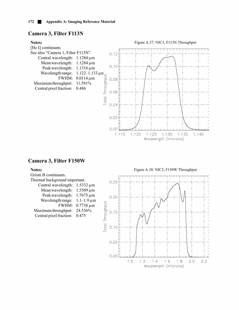
172 Appendix A: Imaging Reference Material
Camera 3, Filter F113N
Camera 3, Filter F150W
Notes:[He I] continuum.See also “Camera 1, Filter F113N”.
Central wavelength: 1.1284 mMean wavelength: 1.1284 mPeak wavelength: 1.1316 m
Wavelength range: 1.122–1.133 mFWHM: 0.0114 m
Maximum throughput: 11.591%Central pixel fraction: 0.486
Figure A.37: NIC3, F113N Throughput
Notes:Grism B continuum.Thermal background important.
Central wavelength: 1.5332 mMean wavelength: 1.5509 mPeak wavelength: 1.7675 m
Wavelength range: 1.1–1.9 mFWHM: 0.7738 m
Maximum throughput: 24.536%Central pixel fraction: 0.475
Figure A.38: NIC3, F150W Throughput

Camera 3, Filter F160W 173
Camera 3, Filter F160W
Camera 3, Filter F164N
Notes:Minimum background.See also “Camera 1, Filter F160W” and“Camera 2, Filter F160W”.
Central wavelength: 1.6036 mMean wavelength: 1.6079 mPeak wavelength: 1.7725 m
Wavelength range: 1.4–1.8 mFWHM: 0.3989 m
Maximum throughput: 23.465%Central pixel fraction: 0.474
Figure A.39: NIC3, F160W Throughput
Notes:[Fe II] line.See also “Camera 1, Filter F164N”.
Central wavelength: 1.6460 mMean wavelength: 1.6460 mPeak wavelength: 1.6476 m
Wavelength range: 1.637–1.655 mFWHM: 0.0173 m
Maximum throughput: 20.234%Central pixel fraction: 0.471
Figure A.40: NIC3, F164N Throughput

174 Appendix A: Imaging Reference Material
Camera 3, Filter F166N
Camera 3, Filter F175W
Notes:[Fe II] continuum.See also “Camera 1, Filter F166N”.
Central wavelength: 1.6583 mMean wavelength: 1.6583 mPeak wavelength: 1.6602 m
Wavelength range: 1.649–1.667 mFWHM: 0.0169 m
Maximum throughput: 20.419%Central pixel fraction: 0.70
Figure A.41: NIC3, F166N Throughput
Notes:Thermal background important.
Central wavelength: 1.805 mMean wavelength: 1.8333 mPeak wavelength: 2.2835 m
Wavelength range: 1.2–2.3 mFWHM: 0.9137 m
Maximum throughput: 31.531%Central pixel fraction: 0.448
Figure A.42: NIC3, F175W Throughput

Camera 3, Filter F187N 175
Camera 3, Filter F187N
Camera 3, Filter F190N
Notes:Paschen line.See also “Camera 1, Filter F187N” and“Camera 2, Filter F187N”.
Central wavelength: 1.8748 mMean wavelength: 1.8748 mPeak wavelength: 1.8756 m
Wavelength range: 1.865–1.884 mFWHM: 0.0191 m
Maximum throughput: 22.56%Central pixel fraction: 0.439
Figure A.43: NIC3, F187N Throughput
Notes:Paschen continuum.See also “Camera 1, Filter F190N” and “Camera 2, Filter F190N”.
Central wavelength: 1.9003 mMean wavelength: 1.9003 mPeak wavelength: 1.9004 m
Wavelength range: 1.892–1.908 mFWHM: 0.0178 m
Maximum throughput: 24.191%Central pixel fraction: 0.434
Figure A.44: NIC3, F190N Throughput

176 Appendix A: Imaging Reference Material
Camera 3, Filter F196N
Camera 3, Filter F200N
Notes:[Si VI].Thermal background important.
Central wavelength: 1.9639 mMean wavelength: 1.9639 mPeak wavelength: 1.9698 m
Wavelength range: 1.954–1.974 mFWHM: 0.0190 m
Maximum throughput: 24.834%Central pixel fraction: 0.424
Figure A.45: NIC3, F196N Throughput
Notes:[Si VI] continuum.Thermal background important.
Central wavelength: 1.9975 mMean wavelength: 1.9975 mPeak wavelength: 2.0022 m
Wavelength range: 1.986–2.007 mFWHM: 0.0209 m
Maximum throughput: 24.012%Central pixel fraction: 0.418
Figure A.46: NIC3, F200N Throughput

Camera 3, Filter F212N 177
Camera 3, Filter F212N
Camera 3, Filter F215N
Notes:H2 line.Thermal background important.See also “Camera 2, Filter F212N”.
Central wavelength: 2.1213 mMean wavelength: 2.1213 mPeak wavelength: 2.1228 m
Wavelength range: 2.111–2.132 mFWHM: 0.0208 m
Maximum throughput: 24.611%Central pixel fraction: 0.396
Figure A.47: NIC3, F212N Throughput
Notes:H2 continuum.Thermal background important.See also “Camera 2, Filter F215N”.
Central wavelength: 2.1487 mMean wavelength: 2.1487 mPeak wavelength: 2.1562 m
Wavelength range: 2.138–2.158 mFWHM: 0.0202 m
Maximum throughput: 23.867%Central pixel fraction: 0.391
Figure A.48: NIC3, F215N Throughput

178 Appendix A: Imaging Reference Material
Camera 3, Filter F222M
Camera 3, Filter F240M
Notes:CO continuum.Thermal background important.See also “Camera 2, Filter F222M”.
Central wavelength: 2.2174 mMean wavelength: 2.2180 mPeak wavelength: 2.1866 m
Wavelength range: 2.15–2.28 mFWHM: 0.1451 m
Maximum throughput: 25.088%Central pixel fraction: 0.380
Figure A.49: NIC3, F222M Throughput
Notes:CO band.Thermal background important.
Central wavelength: 2.3955 mMean wavelength: 2.3963 mPeak wavelength: 2.4130 m
Wavelength range: 2.3–2.5 mFWHM: 0.1951 m
Maximum throughput: 29.697%Central pixel fraction: 0.349
Figure A.50: NIC3, F240M Throughput

APPENDIX B:
Flux Units andLine Lists
In this appendix . . .
B.1 Infrared Flux Units
In the infrared, as in the optical, the means of reporting sourcebrightnesses and the units employed have varied considerably. In recentyears, however, magnitude systems have been used less frequently, and themost popular unit for expressing brightnesses, both for point source fluxesand surface brightnesses, is steadily becoming the Jansky. We have adoptedthe Jansky as the standard flux unit (and Jansky/arcsec2 for surfacebrightness measurements) for NICMOS in our documentation and inobserver-oriented software. Here we provide some simple formulae andtables to facilitate the conversion from other units into Jy
. A Unit Conversion Tool is also available on theNICMOS WWW site, at the following URL:
http://www.stsci.edu/hst/nicmos/tools/conversion_form.html
B.1.1 Some HistoryInfrared astronomy really began in the 1960s, when the vast majority of
astronomy was still carried out in the visual region. Flux measurements
B.1 Infrared Flux Units / 179B.2 Formulae / 181
B.3 Look-up Tables / 182B.4 Examples / 189
B.5 Infrared Line Lists / 189
1Jy 10 26– Wm 2– Hz 1–=
179
180 Appendix B: Flux Units and Line Lists
were routinely reported in the UBV magnitude system, and to attempt tointegrate IR astronomy into this system, Johnson (Ap.J., 134, 69) definedthe first IR magnitude system. This involved four new photometric bands,the J, K, L and M bands which were centered on wavelengths of 1.3, 2.2,3.6 and 5.0 microns. These bands were defined not only by the filterbandpasses, but also by the wavebands of the ‘windows’ of hightransmission through the atmosphere. In this system, all measurementswere referred to the Sun, which was assumed to be a G2V star with aneffective temperature of 5785K, and was taken to have a V–K color ofroughly +2.2. From his own measurements in this system, Johnsondetermined Vega to have a K magnitude of +0.02 and K–L=+0.04.
Until the early 1980s IR astronomical observations were restricted tospectra or single channel photometry, and most photometry was reported insystems at least loosely based on Johnson’s system. These systems added anew band at 1.6 microns known as the H band and two bands weredeveloped in place of the one formerly defined by Johnson as the L band; anew definition of the L band centered on 3.4 microns, and a rathernarrower band known as L' centered on 3.74microns.
As the new science of infrared astronomy rapidly expanded itswavelength coverage, many new photometric bands were adopted, both forground-based observations and for use by the many balloon- androcket-borne observations and surveys. The differing constraints presentedby these different environments for IR telescopes resulted in systems withdisappointingly little commonality or overlap, and today the IR astronomeris left with a plethora of different systems to work with.
The IRAS survey results, which were published in 1986, presentedobservations made photometrically in four bands in the mid- andfar-infrared, and mid-infrared spectra, and all were presented in units ofJanskys, rather than defining yet another new magnitude system. Sincethen, IR data from many sites around the world have been increasinglycommonly presented in Janskys (Jy), or in Jy/arcsec2 in the case of surfacebrightness data. IRAS maps are often presented in units of MJy/steradian.
Ground-based mid-IR photometry is usually carried out using the N andQ photometric bands, which are themselves defined more by theatmospheric transmission than by any purely scientific regard. IRAS, freedof the constraints imposed by the atmosphere, adopted its own 12 micronand 25 micron bands, which were extremely broad and therefore offeredhigh sensitivity. Similarly, NICMOS, being above the atmosphere, is notforced to adopt filter bandpasses (See Chapter 4 and Appendix A) likethose used at ground-based observatories, but instead has filtersconstrained purely by the anticipated scientific demands. Thus in practiceNICMOS does not have filters precisely matched to any of the standardground-based photometric bands. The remaining sections contain simpleformulae to convert between systems (magnitudes to Jy, etc.) and look uptables.

Formulae 181
B.2 Formulae
B.2.1 Converting Between F and FOne Jansky (Jy) is defined as 10–26Wm-2Hz-1, so it is a unit of
measurement of the spectral flux density, F.To determine F from F in Jy, use the following formula:
where is the wavelength in microns (m), and is a constant chosenfrom Table B.1 and depending on the units of F. (This is simply derived,using the fact that d/d = c/2.)
Remember that 1W=107erg sec-1, and 1m=104Å.
B.2.2 Conversion Between Fluxes and MagnitudesThe spectral flux density F can be calculated from its magnitude as
where m is the magnitude and Fo the zero-point flux for the givenphotometric band. We list the central wavelengths and zero-point fluxes forthe more commonly encountered photometric bands below in Table B.2.The CIT system was originally based on Beckwith et al. (1976, Ap.J., 208,390); the UKIRT system is in fact based on the original CIT system, butwith adjustments made largely owing to different filter bandpasses. Itshould be noted that for a given photometric band there will be smalldifferences in the effective wavelength and zero-point flux from one
Table B.1: Constants for Converting F and F
F measured in
Wm-2m-1 310–12
Wcm-2m-1 310–16
erg sec-1 cm-2 m-1 310–9
erg sec-1 cm-2 Å-1 310–13
F F 2=
F 10m– 2.5
Fo=

182 Appendix B: Flux Units and Line Lists
observatory to another, and for astronomical objects with radicallydifferent colors, so these figures can only be treated as approximate.
B.2.3 Conversion Between Surface Brightness UnitsSurface brightnesses are generally measured in Janskys arcsec-2, MJy
steradian-1 or magnitudes arcsec-2. If you have a surface brightness S inMJy steradian-1, then you can use:
.If you have S in magnitudes arcsec-2, you can simply use the formula andzero-points as given in the previous section for point sources.
B.3 Look-up Tables
In this section we provide look-up tables to facilitate rapid, approximateconversion between the different systems mentioned in the precedingsection. IT is important to note that the precise values will change as thesensitivity of NICMOS continually changes. Users should follow theformulas above to generate their own data while keeping in mind that theircalculated values should be close to those provided here.
For both integrated source fluxes and surface brightnesses, we providetables of conversions between systems at the wavelengths of the fourcommonly used photometric bands, which cover the NICMOS operating
Table B.2: Effective Wavelengths and Zero-points for Photometric Bands.
Band [m]Fo[Jy](CIT)
Fo[Jy](UKIRT)
V 0.56 3540 3540
R 0.70 2870 —
I 0.90 2250 —
J 1.25 1670 1600
H 1.65 980 1020
K 2.2 620 657
L 3.4 280 290
L' 3.74 — 252
M 4.8 150 163
N 10.1 37 39.8
Q 20.0 10 10.4
S Jy arcsec2– S MJy ster
1– 2.35 105–=

Look-up Tables 183
waveband of 0.8–2.5 microns. We are adopting here the CIT systemdefined in Table B.2.
Using Table B.3, it is possible to estimate the CIT magnitudecorresponding to any flux in Jy by using the property that multiplying ordividing the flux by one hundred adds or subtracts five magnitudes.
Table B.3: F to Magnitude Conversion.
F [Jy] I J H K
10.0 5.88 5.56 4.98 4.48
8.0 6.12 5.80 5.22 4.72
6.0 6.44 6.11 5.53 5.04
5.0 6.63 6.31 5.73 5.23
4.0 6.88 6.55 5.97 5.48
3.0 7.19 6.86 6.29 5.79
2.5 7.39 7.06 6.48 5.99
2.0 7.63 7.30 6.73 6.23
1.5 7.94 7.62 7.04 6.54
1.25 8.14 7.81 7.24 6.74
1.0 8.38 8.06 7.48 6.98
0.8 8.62 8.30 7.72 7.22
0.6 8.94 8.61 8.03 7.54
0.5 9.13 8.81 8.23 7.73
0.4 9.38 9.05 8.47 7.98
0.3 9.69 9.36 8.79 8.29
0.25 9.89 9.57 8.98 8.49
0.2 10.13 9.8 9.23 8.73
0.15 10.44 10.12 9.54 9.04
0.125 10.64 10.31 9.74 9.24
0.1 10.88 10.56 9.98 9.48

184 Appendix B: Flux Units and Line Lists
Table B.4: I-Band Flux Conversion.
F [Jy]
I [mag]
F[Wm-2m-1]
F[W cm-2m-1]
F[erg s-1 cm-2 Å-1]
2250 0.0 8.3210–9 8.3210–13 8.3210–10
894 1.0 3.31210–9 3.31210–13 3.31210–10
356 2.0 1.31910–9 1.31910–13 1.31910–10
142 3.0 5.2510–10 5.2510–14 5.2510–11
56.4 4.0 2.0910–10 2.0910–14 2.0910–11
22.5 5.0 8.3210–11 8.3210–15 8.3210–12
8.94 6.0 3.31210–11 3.31210–15 3.31210–12
3.56 7.0 1.31910–11 1.31910–15 1.31910–12
1.42 8.0 5.2510–12 5.2510–16 5.2510–13
0.564 9.0 2.0910–12 2.0910–16 2.0910–13
0.225 10.0 8.3210–13 8.3210–17 8.3210–14
0.0894 11.0 3.31210–13 3.31210–17 3.31210–14
0.0356 12.0 1.31910–13 1.31910–17 1.31910–14
0.0142 13.0 5.2510–14 5.2510–18 5.2510–15
0.00564 14.0 2.0910–14 2.0910–18 2.0910–15
0.00225 15.0 8.3210–15 8.3210–19 8.3210–16
8.9410–4 16.0 3.31210–15 3.31210–19 3.31210–16
3.5610–4 17.0 1.31910–15 1.31910–19 1.31910–16
1.4210–4 18.0 5.2510–16 5.2510–20 5.2510–17
5.6410–5 19.0 2.0910–16 2.0910–20 2.0910–17
2.2510–5 20.0 8.3210–17 8.3210–21 8.3210–18
8.9410–6 21.0 3.31210–17 3.31210–21 3.31210–18
3.5610–6 22.0 1.31910–17 1.31910–21 1.31910–18
1.4210–6 23.0 5.2510–18 5.2510–22 5.2510–19
5.6410–7 24.0 2.0910–18 2.0910–22 2.0910–19
2.2510–7 25.0 8.3210–19 8.3210–23 8.3210–20
8.9410–8 26.0 3.31210–19 3.31210–23 3.31210–20

Look-up Tables 185
Table B.5: J-band Flux Conversion.
F[Jy]
J[mag]
F[Wm-2m-1]
F[Wcm-2m-1]
F[erg cm-2s-1Å-1]
1670 0.0 3.2110–9 3.2110–13 3.2110–10
665 1.0 1.2810–9 1.2810–13 1.2810–10
265 2.0 5.0810–10 5.0810–14 5.0810–11
106 3.0 2.0210–10 2.0210–14 2.0210–11
42.0 4.0 8.0610–11 8.0610–15 8.0610–12
16.7 5.0 3.2110–11 3.2110–15 3.2110–12
6.65 6.0 1.2810–11 1.2810–15 1.2810–12
2.65 7.0 5.0810–12 5.0810–16 5.0810–13
1.06 8.0 2.0210–12 2.0210–16 2.0210–13
0.420 9.0 8.0610–13 8.0610–17 8.0610–14
0.167 10.0 3.2110–13 3.2110–17 3.2110–14
0.0665 11.0 1.2810–13 1.2810–17 1.2810–14
0.0265 12.0 5.0810–14 5.0810–18 5.0810–15
0.0106 13.0 2.0210–14 2.0210–18 2.0210–15
0.00420 14.0 8.0610–15 8.0610–19 8.0610–16
0.00167 15.0 3.2110–15 3.2110–19 3.2110–16
6.6510–4 16.0 1.2810–15 1.2810–19 1.2810–16
2.6510–4 17.0 5.0810–16 5.0810–20 5.0810–17
1.0610–4 18.0 2.0210–16 2.0210–20 2.0210–17
4.2010–5 19.0 8.0610–17 8.0610–21 8.0610–18
1.6710–5 20.0 3.2110–17 3.2110–21 3.2110–18
6.6510–6 21.0 1.2810–17 1.2810–21 1.2810–18
2.6510–6 22.0 5.0810–18 5.0810–22 5.0810–19
1.0610–6 23.0 2.0210–18 2.0210–22 2.0210–19
4.2010–7 24.0 8.0610–19 8.0610–23 8.0610–20
1.6710–7 25.0 3.2110–19 3.2110–23 3.2110–20
6.6510–8 26.0 1.2810–19 1.2810–23 1.2810–20

186 Appendix B: Flux Units and Line Lists
Table B.6: H-band Flux Conversion.
F[Jy]
H[mag]
F[Wm-2m-1]
F[Wcm-2m-1]
F[erg s-1cm-2Å-1]
980 0.0 1.0810–9 1.0810–13 1.0810–10
390 1.0 4.310–10 4.310–14 4.310–11
155 2.0 1.71210–10 1.71210–14 1.71210–11
61.8 3.0 6.81410–11 6.81410–15 6.81410–12
24.6 4.0 2.71310–11 2.71310–15 2.71310–12
9.8 5.0 1.0810–11 1.0810–15 1.0810–12
3.9 6.0 4.310–12 4.310–16 4.310–13
1.55 7.0 1.71210–12 1.71210–16 1.71210–13
0.618 8.0 6.81410–13 6.81410–17 6.81410–14
0.246 9.0 2.71310–13 2.71310–17 2.71310–14
0.098 10.0 1.0810–13 1.0810–17 1.0810–14
0.039 11.0 4.310–14 4.310–18 4.310–15
0.0155 12.0 1.71210–14 1.71210–18 1.71210–15
0.00618 13.0 6.81410–15 6.81410–19 6.81410–16
0.00246 14.0 2.71310–15 2.71310–19 2.71310–16
9.810–4 15.0 1.0810–15 1.0810–19 1.0810–16
3.910–4 16.0 4.310–16 4.310–20 4.310–17
1.5510–4 17.0 1.71210–16 1.71210–20 1.71210–17
6.1810–5 18.0 6.81410–17 6.81410–21 6.81410–18
2.4610–5 19.0 2.71310–17 2.71310–21 2.71310–18
9.810–6 20.0 1.0810–17 1.0810–21 1.0810–18
3.910–6 21.0 4.310–18 4.310–22 4.310–19
1.5510–6 22.0 1.71210–18 1.71210–22 1.71210–19
6.1810–7 23.0 6.81410–19 6.81410–23 6.81410–20
2.4610–7 24.0 2.71310–19 2.71310–23 2.71310–20
9.810–8 25.0 1.0810–19 1.0810–23 1.0810–20
3.910–8 26.0 4.310–20 4.310–24 4.310–21

Look-up Tables 187
Table B.7: K-band Flux Conversion.
F[Jy]
K[mag]
F[Wm-2m-1]
F[Wcm-2m-1]
F[erg s-1cm-2Å-1]
620 0.0 3.8410–10 3.8410–14 3.8410–11
247 1.0 1.5310–10 1.5310–14 1.5310–11
98.3 2.0 6.0910–11 6.0910–15 6.0910–12
39.1 3.0 2.4310–11 2.4310–15 2.4310–12
15.6 4.0 9.6610–12 9.6610–16 9.6610–13
6.20 5.0 3.8410–12 3.8410–16 3.8410–13
2.47 6.0 1.5310–12 1.5310–16 1.5310–13
0.983 7.0 6.0910–13 6.0910–17 6.0910–14
0.391 8.0 2.4310–13 2.4310–17 2.4310–14
0.156 9.0 9.6610–14 9.6610–18 9.6610–15
0.0620 10.0 3.8410–14 3.8410–18 3.8410–15
0.0247 11.0 1.5310–14 1.5310–18 1.5310–15
0.00983 12.0 6.0910–15 6.0910–19 6.0910–16
0.00391 13.0 2.4310–15 2.4310–19 2.4310–16
0.00156 14.0 9.6610–16 9.6610–20 9.6610–17
6.2010–4 15.0 3.8410–16 3.8410–20 3.8410–17
2.4710–4 16.0 1.5310–16 1.5310–20 1.5310–17
9.8310–5 17.0 6.0910–17 6.0910–21 6.0910–18
3.9110–5 18.0 2.4310–17 2.4310–21 2.4310–18
1.5610–5 19.0 9.6610–18 9.6610–22 9.6610–19
6.2010–6 20.0 3.8410–18 3.8410–22 3.8410–19
2.4710–6 21.0 1.5310–18 1.5310–22 1.5310–19
9.8310–7 22.0 6.0910–19 6.0910–23 6.0910–20
3.9110–7 23.0 2.4310–19 2.4310–23 2.4310–20
1.5610–7 24.0 9.6610–20 9.6610–24 9.6610–21
6.2010–8 25.0 3.8410–20 3.8410–24 3.8410–21
2.4710–8 26.0 1.5310–20 1.5310–24 1.5310–21

188 Appendix B: Flux Units and Line Lists
Table B.8: Surface Brightness Conversion.
mag /arcsec2
I-Band J-Band H-Band K-Band
Jy /arcsec2
MJy /steradian
Jy /arcsec2
MJy /steradian
Jy /arcsec2
MJy /steradian
Jy /arcsec2
MJy /steradian
0.0 0.6251 2.66104 0.4630 1.97104 0.2726 1.16104 0.1720 7320
1.0 0.2491 1.06104 0.1847 7860 0.1083 4610 0.0688 2930
2.0 0.0989 4210 0.0736 3130 0.0430 1830 0.0273 1160
3.0 0.0395 1680 0.0294 1250 0.0172 730 0.0109 462
4.0 0.0157 667 0.0117 496 0.0068 291 0.0043 184
5.0 0.0062 266 0.0046 197 0.0027 116 0.0172 732
6.0 0.0025 106 0.0018 78.6 0.0011 46.1 6.8810–4 29.3
7.0 9.8910–4 42.1 7.3610–4 31.3 4.3010–4 18.3 2.7310–4 11.6
8.0 3.9510–4 16.8 2.9410–4 12.5 1.7210–4 7.3 1.0910–4 4.62
9.0 1.5710–4 6.67 1.1710–4 4.96 6.8410–5 2.91 4.3210–5 1.84
10.0 6.2510–5 2.66 4.6310–5 1.97 2.7310–5 1.16 1.7210–5 0.732
11.0 2.4910–5 1.06 1.8510–5 0.786 1.0810–5 0.461 6.8810–6 0.293
12.0 9.8910–6 0.421 7.3610–6 0.313 4.3010–6 0.183 2.7310–7 0.116
13.0 3.9510–6 0.168 2.9410–6 0.125 1.7210–6 0.073 1.0910–7 0.0462
14.0 1.5710–6 0.0667 1.1710–6 0.0496 6.8410–7 0.0291 4.3210–8 0.0184
15.0 6.2510–7 0.0266 4.6310–7 0.0197 2.7310–7 0.0116 1.7210–8 0.00732
16.0 2.4910–7 0.0106 1.8510–7 0.00786 1.0810–7 0.00461 6.8810–9 0.00293
17.0 9.8910–8 0.00421 7.3610–8 0.00313 4.3010–8 0.00183 2.7310–9 0.00116
18.0 3.9510–8 0.00168 2.9410–8 0.00125 1.7210–8 7.310–4 1.0910–9 4.6210–4
19.0 1.5710–8 6.6710–4 1.1710–8 4.9610–4 6.8410–9 2.9110–4 4.3210–10 1.8410–4
20.0 6.2510–9 2.6610–4 4.6310–9 1.9710–4 2.7310–9 1.1610–4 1.7210–10 7.3210–5
21.0 2.4910–9 1.0610–4 1.8510–9 7.8610–5 1.0810–9 4.6110–5 6.8810–11 2.9310–5
22.0 9.8910–10 4.2110–5 7.3610–10 3.1310–5 4.3010–10 1.8310–5 2.7310–11 1.1610–5
23.0 3.9510–10 1.6810–5 2.9410–10 1.2510–5 1.7210–10 7.310–6 1.0910–11 4.6210–6
24.0 1.5710–10 6.6710–6 1.1710–10 4.9610–6 6.8410–11 2.9110–6 4.3210–12 1.8410–6
25.0 6.2510–11 2.6610–6 4.6310–11 1.9710–6 2.7310–11 1.1610–6 1.7210–12 7.3210–7
26.0 2.4910–11 1.0610–6 1.8510–11 7.8610–7 1.0810–11 4.6110–7 6.8810–13 2.9310–7

Examples 189
B.4 Examples
1. Given a source with a flux of 0.9mJy at 1350Å, convert this flux toerg s-1cm-2Å-1. From section 3, Table B.1, we see that the conversionconstant is 310–13 and the wavelength is 1350Å = 0.135m.Thus:
2. Given a V magnitude of 15.6, and knowledge that V–K=2.5 in theUKIRT system, estimate the flux in Jy at K. Since V–K=2.5 we knowthat K=13.1. From Table B.2, the zero-point flux in the UKIRT sys-tem for K is 657Jy. Thus the 2.2m flux is:
3. Given a surface brightness of 21.1 magnitudes arcsec-2 at J, convertthis into Jy arcsec-2. Taking the zero-point for the J band from TableB.2, we determine that the surface brightness is:
4. Given a flux at 0.9m of 2.310–7Jy, estimate the I magnitude.2.310–7Jy is less than 2.310–1Jy by three powers of a hundred, or15 magnitudes. From Table B.3 we see that 0.25Jy is equivalent to anI-band magnitude of 9.89. Thus 2.310–7 is roughly 15 magnitudesfainter than this, or of order:
B.5 Infrared Line Lists
We present here lists of some of the more important atomic andmolecular lines in the infrared. It is by no means exhaustive.
F 3 1013– 9 10
4– 0.1352 1.48 10
14–erg s
1– cm
2–Å
1–= =
F 10-13.1/2.5
657 3.8 103–Jy= =
10-21.1/2.5
1670 6.06 106–Jy arcsec
2–=
I 24.9=

190 Appendix B: Flux Units and Line Lists
Table B.9: Recombination Lines of Atomic Hydrogen: Paschen Series1.
Transition(Nu - Nl)
Vacuum Wavelength(microns)
Vacuum Frequency(cm -1)
I/I(H)Te=Ne=104
4-3 1.8756 5531.55 0.332
5-3 1.2822 7799.33 0.162
6-3 1.0941 9139.8 0.0901
7-3 1.0052 9948.1
1. Intensities from Hummer & Storey, MNRAS 224, 801.
Table B.10: Recombination Lines of Atomic Hydrogen: Brackett Series.
Transition(Nu-Nl)
Vacuum Wavelength(microns)
Frequency(cm -1)
I/I(H)Te=104
5-4 4.5225 2467.765 0.0777
6-4 2.6259 3808.25
7-4 2.1661 4616.61 0.0275
8-4 1.9451 5141.14 0.0181
9-4 1.8181 5500.8 0.0126
10-4 1.7367 5758.1 0.00909
11-4 1.6811 5948.45 0.00679
12-4 1.6412 6093.22 0.00521
13-4 1.6114 6205.9 0.00409
14-4 1.5885 6295.3 0.00327
15-4 1.5705 6367.4 0.00266
16-4 1.5561 6426.4 0.00220
17-4 1.5443 6475.3 0.00184
18-4 1.5346 6516.3 0.00156
19-4 1.5265 6551.0 0.00133
20-4 1.5196 6580.7 0.00116
series limit 1.459 6855.

Infrared Line Lists 191
Table B.11: HeI and HeII Lines.
ID Transition (m)
HeI 7F-3D,3Fo-3D 1.0031
HeI 7F-3D,1Fo-1D 1.0034
HeII 14-6 1.0049
HeII 5-4 1.0133
HeI 6D-3P,3dD-3Po 1.0314
HeII 13-6 1.0422
HeI 6S-3P,3S-3Po 1.0668
HeI 2P-2S,3Po-3S,GU=3 1.0832
HeI 2P-2S,3Po-3P,GU=1 1.0832
HeI 2P-2S,3Po-3S,GU=5 1.0833
HeI 2P-2S,3Po-3S,GU=9 1.0833
HeI 6P-3D,1Po-1d 1.0905
HeI 6F-3D,3Fo-3D 1.0916
HeI 6F-3D,1Fo-1D 1.0920
HeII 12-6 1.0938
HeI 6P-3D,3Po-3D 1.0997
HeI 5P-3S,1Po-1S 1.1016
HeI 6D-3P,1D-1Po 1.1048
HeII 7LIMIT 1.1164
HeI 6S-3P,1S-1Po 1.1229
HeII 7-5 1.1628
HeII 11-6 1.1677
HeI 5D-3P,3D-3Po 1.1972
HeII 21-7 1.2256
HeII 22-7 1.2418
HeI 4P-3S,3Po-3S 1.2531
HeII 20-7 1.2719
HeI 5P-3D,1Po-1D 1.2759
HeI 5F-3D,3Fo-3D 1.2789
HeII 10-6 1.2817
HeI 5S-3P,3S-3Po 1.2850

192 Appendix B: Flux Units and Line Lists
HeII 19-7 1.2914
HeI 5D-3P,1D-1Po 1.2971
HeI 5F-3D,1Fo-1D 1.2976
HeI 5P-3D,3Po-3D 1.2988
HeII 18-7 1.3150
HeI 5S-3P,1S-1Po 1.3415
HeII 17-7 1.3442
HeII 15-7 1.4273
HeII 8LIMIT 1.4578
HeII 9-6 1.4765
HeII 14-7 1.4882
HeI 4P-3S,1Po-1S 1.5088
HeII 13-7 1.5719
HeII 25-8 1.6241
HeII 24-8 1.6400
HeII 23-8 1.6584
HeII 22-8 1.6799
HeII 12-7 1.6926
HeI 4D-3P,3D-3Po 1.7007
HeII 21-8 1.7053
HeII 20-8 1.7355
HeII 19-8 1.7717
HeII 18-8 1.8167
HeII 9LIMIT 1.8450
HeI 4P-3D,1Po-1D 1.8561
HeII 6-5 1.8639
HeI 4F-3D,3Fo-3D 1.8691
HeI 4F-3D,1Fo-1d 1.8702
HeII 17-8 1.8725
HeII 8-6 1.8753
HeII 11-7 1.8770
Table B.11: HeI and HeII Lines. (Continued)
ID Transition (m)

Infrared Line Lists 193
HeI 8S-4P,3S-3Po 1.9068
HeI 4D-3P,1D-1Po 1.9094
HeI 4P-3D,3Po-3D 1.9548
HeII 15-8 2.0379
HeI 6P-4S,3Po-3S 2.0430
HeI 2P-2S,1Po-1S 2.0587
HeI 4S-3P,3S-3Po 2.1126
HeI 3pP-4sS 2.1132
HeI 4S-3P,1S-1Po 2.1138
HeII 25-9 2.1195
HeII 24-9 2.1469
HeI 7S-4P,3S-3Po 2.1500
HeI 7F-4D,3Fo-3D 2.1614
HeI 4dD-7fF 2.1617
HeI 7F-4D,1Fo-1D 2.1623
HeII 14-8 2.1653
HeI 4-7 2.166
HeII 23-9 2.1786
HeI 7D-4P,1D-1Po 2.1847
HeII 10-7 2.1891
HeII 22-9 2.2155
HeI 7S-4P,1S-1Po 2.2290
HeII 21-9 2.2601
HeII 10LIMIT 2.2778
HeI 6P-4S,1Po-1S 2.3069
HeII 20-9 2.314
HeII 13-8 2.348
HeII 19-9 2.3788
HeII 18-9 2.4606
HeI 6D-4P,3D-3Po 2.4734
Table B.11: HeI and HeII Lines. (Continued)
ID Transition (m)

194 Appendix B: Flux Units and Line Lists
Table B.12: CO Vibration-rotation Band-heads1.
1. All of the delta v = 2 bandheads occur near J=50.
Transition(Nu-Nl)
12C16OVacuum Wavelength(microns)
Frequency(cm -1)
13C16OVacuum Wavelength(microns)
Frequency(cm -1)
2-0 2.2935 4360.1 2.3448 4264.7
3-1 2.3227 4305.4 2.3739 4212.4
4-2 2.3535 4250.8 2.4037 4160.3
5-3 2.3829 4196.5 2.4341 4108.3
6-4 2.4142 4142.2 2.4652 4056.4
7-5 2.4461 4088.2 2.4971 4004.7
8-6 2.4787 4034.3
9-7 2.5122 3980.5
3-0 1.5582 6417.8
4-1 1.5780 6337.2
5-2 1.5982 6257.2
6-3 1.6187 6177.7
7-4 1.6397 6098.8
8-5 1.6610 6020.5

Infrared Line Lists 195
Table B.13: Important H2 Lines1.
Line NameWavel(m)
Freq(cm-1)
g(J)Eupper
(K)A
(10e-7s)
LTE I(line)/I(1-0S(1))
1000K 2000K 3000K 4000K
1-0 S(0) 2.2235 4497.41 5 6471 2.53 0.27 0.21 0.19 0.19
1-0 S(1) 2.1218 4712.91 21 6956 3.47 1.00 1.00 1.00 1.00
1-0 S(2) 2.0338 4917.01 9 7584 3.98 0.27 0.37 0.42 0.44
1-0 S(3) 1.9576 5108.40 33 8365 4.21 0.51 1.02 1.29 1.45
1-0 S(4) 1.8920 5282.52 13 9286 4.19 0.082 0.26 0.39 0.47
1-0 S(5) 1.8358 5447.25 45 10341 3.96 0.096 0.52 0.91 1.21
1-0 S(6) 1.7880 5592.9 17 11522 3.54 0.010 0.10 0.21 0.31
1-0 S(7) 1.7480 5720.8 57 12817 2.98 0.008 0.15 0.40 0.65
1-0 S(8) 1.7147 5831.9 21 14221 2.34 0.001 0.022 0.074 0.14
1-0 S(9) 1.6877 5925.1 69 15722 1.68 0.025 0.11 0.22
1-0 S(10) 1.6665 6000.0 25 17311 1.05 0.003 0.015 0.034
1-0 S(11) 1.6504 6059.0 81 18979 0.53 0.002 0.014 0.037
1-0 Q(1) 2.4066 4155.25 9 6149 4.29 1.05 0.70 0.61 0.57
1-0 Q(2) 2.4134 4143.47 5 6471 3.03 0.30 0.23 0.22 0.21
1-0 Q(3) 2.4237 4125.87 21 6956 2.78 0.70 0.70 0.70 0.70
1-0 Q(4) 2.4375 412.57 9 7586 2.65 0.15 0.21 0.23 0.24
1-0 Q(5) 2.4548 4073.72 33 8365 2.55 0.24 0.49 0.62 0.70
1-0 Q(6) 2.4756 4039.5 13 9286 2.45 0.036 0.12 0.17 0.21
1-0 Q(7) 2.5001 3999.9 45 10341 2.34 0.042 0.11 0.40 0.53
3-2 S(0) 2.5014 3997.73 5 17387 3.88 0.001 0.007 0.016
3-2 S(1) 2.3864 4190.33 21 17818 5.14 0.006 0.035 0.087
3-2 S(2) 2.2870 4372.49 9 18386 5.63 0.002 0.014 0.037
3-2 S(3) 2.2014 4542.57 33 19086 5.63 0.006 0.043 0.12
3-2 S(4) 2.1280 4699.32 13 19912 5.22 0.001 0.012 0.036
3-2 S(5) 2.0656 4841.3 45 20856 4.50 0.003 0.023 0.088
3-2 S(6) 2.0130 4967.7 17 21911 3.57 0.006 0.021
3-2 S(7) 1.9692 5078.1 57 23069 2.54 0.001 0.010 0.038
4-3 S(3) 2.3446 4265.4 21
4-3 S(4) 2.2668 4411.5 9
4-3 S(5) 2.201 4543.5 33

196 Appendix B: Flux Units and Line Lists
5-4 S(5) 2.3555 4245.4 45
5-4 S(7) 2.2510 4442.5 57
2-0 S(0) 1.2383 8075.3 5 12095 1.27 0.001 0.012 0.028 0.043
2-0 S(1) 1.1622 8604.2 21 12550 1.90 0.004 0.061 0.15 0.23
2-0 S(2) 1.1382 8785.5 9 13150 2.38 0.001 0.025 0.070 0.12
2-0 S(3) 1.1175 8948.6 33 13890 2.77 0.002 0.074 0.24 0.43
2-0 S(4) 1.0998 9092.4 13 14764 3.07 0.021 0.078 0.15
2-0 S(5) 1.0851 9215.5 45 15763 3.28 0.001 0.048 0.21 0.44
2-9 Q(1) 1.2383 8075.3 9 11789 1.94 0.003 0.037 0.082 0.12
2-0 Q(2) 1.2419 8051.9 5 12095 1.38 0.001 0.012 0.029 0.045
2-0 Q(3) 1.2473 8017.2 21 12550 1.29 0.002 0.039 0.098 0.24
2-0 Q(4) 1.2545 7971.1 9 13150 1.27 0.001 0.012 0.033 0.056
2-0 Q(5) 1.2636 7913.3 33 13890 1.23 0.001 0.024 0.093 0.17
2-0 O(2) 1.2932 7732.6 1 11635 3.47 0.001 0.008 0.016 0.024
2-0 O(3) 1.3354 7488.3 9 11789 1.61 0.003 0.028 0.063 0.094
2-0 O(4) 1.3817 7237.5 5 12095 1.03 0.001 0.008 0.020 0.030
2-0 O(5) 1.4322 6982.5 21 12550 0.698 0.001 0.018 0.046 0.074
1. Energy levels calculated using Dabrowski & Herzberg, Can J Phys 62, 1639 (1984). Einstein coefficients from Turner et al. ApJ Suppl 35, 281 (1977).
Table B.13: Important H2 Lines1. (Continued)
Line NameWavel(m)
Freq(cm-1)
g(J)Eupper
(K)A
(10e-7s)
LTE I(line)/I(1-0S(1))
1000K 2000K 3000K 4000K

APPENDIX C:
Bright Object ModeIn this appendix . . .
C.1 Bright Object Mode
The time taken to read through a quadrant on the array sets afundamental limit on the fastest electron collection rate which can beachieved by resetting all the pixels. An inherent consequence of themethods of operating the NICMOS array detectors in the MULTIACCUMand ACCUM modes is, therefore, that there is a minimum possible exposuretime, 0.203 seconds (~ 0.6 seconds for ACCUM), set by the time required toread the array. Although the detector arrays are multiplexed by divisioninto four quadrants, each pixel in a 128 128 pixel quadrant must besampled in some order (note that there is no transfer of charge as is done ina CCD). For a very bright object, the time between the reset of a pixel andits final read is sufficiently long that the pixel saturates.
The solution adopted to this problem for NICMOS is the provision of abright object mode which enables targets to be observed which are ~200
C.1 Bright Object Mode / 197
The use of this read-out mode is recommended only for the purpose ofdetermining the centroid of very bright targets which must be acquiredunder the coronagraphic spot, when any other configuration (e.g.,MULTIACCUM or ACCUM with narrow-band filters) saturates thedetector. Any other use is strongly discouraged, because of the strongnon-linearity of this mode.
197
198 Appendix C: Bright Object Mode
times brighter than is possible in the other modes without saturating. InBRIGHTOBJ mode, an ACCUM sequence of operations is performed on onepixel in each quadrant at a time. That is, the pixel is reset, read, integrated,and read again with the difference between the final and initial readoutsbeing stored as the measured signal and the interval between the readsbeing the exposure time. This process is repeated sequentially for all pixelsin each quadrant. Users can think of this as integrating on a single pixel at atime. The smallest integration time which can be used is 1.024milliseconds, the longest 0.261 seconds. Figure C.1 illustrates theoperation of bright object mode. Initially, the entire detector is reset. Thenthe first pixel (solid shading) in each quadrant is read. After the requestedintegration time, the first pixel in each quadrant is read again. Then thesecond pixel in each quadrant is reset, then read, integrated, and read again.The process continues until all 16,384 pixels in each quadrant have beenread twice, separated by the integration time. The image down linked ismade up of the difference between the two reads of each pixel.
The time required to take a BRIGHTOBJ mode exposure can be ratherlong. Since photons are only collected in one pixel per quadrant at a time,the time associated with obtaining the frame is
where EXPTIME is the integration timeper pixel (i.e. the observation time is approximately (1282) the exposuretime). For example, if an integration time of 0.1 seconds is used to observea bright target then the actual time required to complete the observationwould be around 27 minutes! This means that, allowing for acquisitiontime, only two such exposures can be obtained in a single target visibilityperiod. However, it is not always so serious. In the case of Jupiter, forexample, the integration times required per pixel are only of the order ofmilliseconds and so the total integration time will only be around 20seconds.
The longest exposure time which is possible in BRIGHTOBJ mode is0.261 seconds, requiring 4278 seconds in total. Thus it is possible, in theworst case, for a single BRIGHTOBJ mode exposure to use more than anorbit. In general, observers are strongly advised to consider the trade-offbetween relatively long BRIGHTOBJ mode exposures (which take thelongest time) and short MULTIACCUM mode exposures (using a narrowfilter).
10.0 EXPTIME 16384 +

Bright Object Mode 199
Figure C.1: Bright Object Mode Operation
The advantage of this mode of operation is the ability to acquire objectssignificantly brighter than the normal saturation limit of the detector.
The disadvantages are several:
• The zeropoint in this mode is strongly non-linear, such non-linearity has not been characterized (nor are there plans to do so). Observa-tions obtained with this mode are not calibrated and possibly not eas-ily calibrated.
• Some observations will take a long time. BRIGHTOBJ mode expo-sures are therefore very sensitive to the quality of the pointing of HST. If the object changes (planetary rotation) or if the telescope pointing changes, it will affect different parts of the image differently.
• The D.C. offset of the detector output is not directly removed in this mode of operation. In general, the signal is very high and the offset does not matter. In some cases it will and this can be a detriment to the signal accuracy.
• There is also no cosmic ray correction or saturation detection in this mode of operation. Although they are still susceptible to cosmic rays, events are expected to be very rare as the integration time per pixel is very short.
Res
et
Res
et
Res
et
Res
et
Res
et
128 128
Pixel 1 read out Pixel 2 read out
Pixel 16384 read out
Pixel 3 read out
Pixel 16383 read out

APPENDIX D:
Techniques for Dithering,Background
Measurement andMapping
In this chapter...
D.1 Introduction / 202
D.2 Strategies For Background Subtraction / 204
D.3 Chop and Dither Patterns / 206
D.4 Examples / 213
D.5 Types of Motions / 216
NICMOS patterns have been created to enable observers to performdithering, chopping, and mapping, and these patterns are significantlydifferent than those described in earlier versions of this handbook.
201
202 Appendix D: Techniques for Dithering, Background Measurement and Mapping
D.1 Introduction
Multiple exposures with small offsets in the pointing of the telescopebetween exposures are recommended for NICMOS observations. Wedistinguish three particular circumstances which may require small offsets:
• Dithering to permit the removal of dead or non-calibrated (i.e., non-correctable) pixels on the detectors, and to improve spatial sam-pling and mitigate the effects of detector’s non-uniformities (i.e. sen-sitivity variations),
• Chopping to measure the background associated with an astronomi-cal source, and
• Mapping to map a source larger than a single detector field of view.
The techniques described in this appendix may be used to accomplishany one or any combination of these goals.
Experience with NICMOS has shown that the background is spatiallyuniform (variations no larger than a few percent across the NIC3 field ofview) and does not vary much with time (variations of less than 5% onorbit timescales). The description of the thermal background in Chapter 4,Chapter 9 and the Exposure Time Calculator provide a basis for estimatingthe relative contributions of source and background. It is strongly advisedthat provision for direct measurement of the background be included inproposals whenever observations at wavelengths greater than 1.7m areperformed. The frequency of such measurements should be about once perorbit, and more frequent measurements should be planned when thebackground must be measured to high accuracy.
Background images are obtained by offsetting the telescope from thetarget to point to an “empty” region of the sky. The ability to routinelyoffset the telescope pointing is a fundamental operational requirement forNICMOS. Starting in Cycle 9, HST programs use a standard patternsyntax, which replaced the old pattern optional parameters, and the evenolder scan parameters form. The new syntax allows multiple observations(including those with different filters) to be made at each point in thepattern, if desired. Observers should check the “Phase II ProposalInstructions” and APT documentation for instructions on how to set up apattern, and the “pattern parameter form” that describes the motion. Forsimplicity, a set of pre-defined observing patterns has been built; the
Background measurements are recommended for all observations atwavelengths longward of 1.7 m.

Introduction 203
exposures taken under them are combined into one or more associations. Apattern, then, is a set of images of the same astronomical target obtained atpointings offset from each other, e.g. for the purpose of removing bad orgrot-affected pixels from the combined image, for creating backgroundimages, or mapping an extended target. The associations of exposures arecreated for the purpose of simultaneously processing all the images(through a given filter) from a single pattern. Thus, dithered images can beeasily reassembled into a single image with the effects of minimizing badpixels, or images taken in the long wavelength regime can be corrected forthe thermal contribution, or observations of extended targets can becombined into a single large map.
Three distinct types of pattern motion are defined:
• Dither: Individual motions are limited to no more than 40 arcsec. These are intended to be used to perform small dithers, to measure backgrounds for compact sources, and to accomplish sequences of overlapping exposures for the construction of mosaics. Such sequences will be assembled into a single final image by the calibra-tion pipeline.
• Chop: Motions up to 1440 arcsec are permitted. These are intended for the measurement of the background at one or more locations sig-nificantly removed from the target pointing. Non-contiguous back-ground images and target images will be assembled into their own final image by the calibration pipeline.
• Mapping: Large motions comparable to the size of the aperture (e.g. 11, 20, or 50 arcsec) are specified. These are intended to cover large regions of the sky in a regular grid pattern.
Telescope motions involve overheads for physically moving thetelescope and, if necessary, for re-acquiring the guide stars. Therefore,significant time overheads may be incurred by observations which needbackground subtraction or propose to map extended regions of the sky. Acareful estimate of the overheads associated with a specific observation orset of observations is necessary to evaluate the number of orbits required(see Chapter 10).
Starting with Cycle 14, previously unassociated NICMOS observationswithin a visit, using the same detector and filter, are collected into anassociation, provided a POS-TARG is specified on the exposure line.The assignment of association numbers is determined from the APTPhase II file exposure line specifications for each visit. Currently, thenew association assignments are NOT applicable to previously exe-cuted observations, nor does it apply to parallel observations.
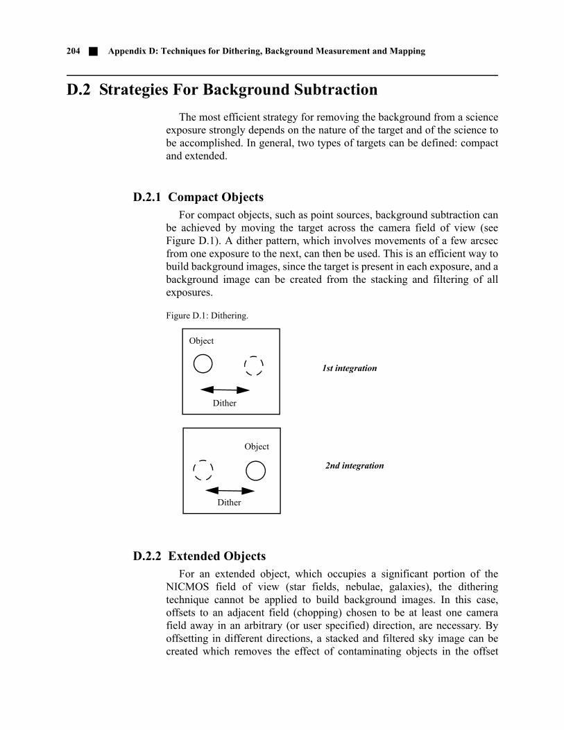
204 Appendix D: Techniques for Dithering, Background Measurement and Mapping
D.2 Strategies For Background Subtraction
The most efficient strategy for removing the background from a scienceexposure strongly depends on the nature of the target and of the science tobe accomplished. In general, two types of targets can be defined: compactand extended.
D.2.1 Compact ObjectsFor compact objects, such as point sources, background subtraction can
be achieved by moving the target across the camera field of view (seeFigure D.1). A dither pattern, which involves movements of a few arcsecfrom one exposure to the next, can then be used. This is an efficient way tobuild background images, since the target is present in each exposure, and abackground image can be created from the stacking and filtering of allexposures.
Figure D.1: Dithering.
D.2.2 Extended ObjectsFor an extended object, which occupies a significant portion of the
NICMOS field of view (star fields, nebulae, galaxies), the ditheringtechnique cannot be applied to build background images. In this case,offsets to an adjacent field (chopping) chosen to be at least one camerafield away in an arbitrary (or user specified) direction, are necessary. Byoffsetting in different directions, a stacked and filtered sky image can becreated which removes the effect of contaminating objects in the offset
Object
Dither
Object
Dither
1st integration
2nd integration

Strategies For Background Subtraction 205
fields (see Figure D.2). As in the case of compact objects, these offsetsmight be quite small, but for large galaxies for example, they may need tobe over considerable distances. The user has the ability to specify the offsetvalue, directions, and the number of offsets in the Phase II patternparameter specification.
Figure D.2: Chopping.
Telescope Offset
Telescope Offsetin Different Direction
Field withcontaminating
Field with
1st Integrationon object
2nd integrationon object
sources
differentcontaminatingsource

206 Appendix D: Techniques for Dithering, Background Measurement and Mapping
D.3 Chop and Dither Patterns
There are a set of fifteen pre-designed patterns available for NICMOSobservations. Users may define their own pattern specifications as well inAPT, during Phase II development. The pre-defined patterns include fourdither patterns, four chop patterns, five dither-chop patterns, and two mappatterns. For each of these, the observer will be able to specify the numberof positions desired (1 to 50), the dither size (0 to 40 arcsec), the chop size(0 to 1440 arcsec, also used for mapping), and the orientation of the patternwith respect to either the detector or the sky. The POS-TARG specialrequirement is still available for offsetting the telescope and creatingcustom-design patterns as well, but there are a number of advantages tousing the pre-designed patterns:
• Patterns simplify the specification of complex observations in the Phase II proposal.
• All the observations pertaining to an exposure specification line in a pattern result in one association and are simultaneously calibrated and combined in the data calibration pipeline, including background calibration, cosmic ray removal, and flat fielding. Observations obtained with POS-TARG do not result in associations, and will have to be combined manually by the observer.
• Patterns permit the observation of a region on the sky with a fixed position angle without fixing spacecraft roll, which increases the number of opportunities to schedule the observations.
Multiple exposures may be obtained at each position by the use of thePhase II exposure level parameter for Iterations. This may be useful forcosmic ray removal. In addition, exposures in different filters at eachpattern position can be obtained by linking together exposure lines as apattern group.
The fifteen NICMOS pre-designed patterns are listed in Table D.1,together with applicable parameters, such as the allowed values for thenumber of steps in the pattern, the dither size, or the chop size. In addition,the figure number where the pattern is graphically shown is given in thelast column of Table D.1. Offset sizes and number of steps in a patternaffect the amount of overhead time required to perform an observation (seeChapter 10). The effects of dithering or chopping on an astronomical imageare shown in a set of examples in the next section.

Chop and Dither Patterns 207
Note on Orientation:The pattern parameter syntax requires additional input on orientation.
Specifically, the pattern must be defined in either the POS-TARG (camera)frame or the CELESTIAL (sky) frame. Dithering to remove detectorcharacteristics should always be performed in the POS-TARG frame ofreference. A pattern orientation angle may be specified as well. In thePOS-TARG frame, this is the angle of the motion of the target from the firstpoint of the pattern to the second, counterclockwise from the x detectoraxis (the directions are defined in Figure 6.1). In the CELESTIAL frame,the angle is measured from North through East.
Note that some of the pattern names in Table D.1 are doubled except foran additional -SKY-. The chop can be specified either as POS-TARG orCELESTIAL (default—see below for details).
Move the sky or the telescope?The pattern syntax attempts to resolve the confusing dichotomy in the
old pattern implementation, as to whether the pattern moves the telescope
Table D.1:NICMOS Pre-designed Observing Patterns and Parameters.
Pattern NameNum.of Dithers
Num.Chops
DitherSize
ChopSize
Orient frame
SeeFigure
NIC-SPIRAL-DITH 1–50 NA 0–40 NA camera D.3
NIC-SQUARE-WAVE-DITH 1–50 NA 0–40 NA camera D.3
NIC-XSTRIP-DITH 1–50 NA 0–40 NA camera D.3
NIC-YSTRIP-DITH 1–50 NA 0–40 NA camera D.3
NIC-ONE-CHOP NA 1–50 NA 0–1440 camera D.4
NIC-TWO-CHOP NA 1–50 NA 0–1440 camera D.4
NIC-SPIRAL-DITH-CHOP 1–50 2 0–40 0–1440 camera D.5
NIC-XSTRIP-DITH-CHOP 1–50 2 0–40 0–1440 camera D.5
NIC-YSTRIP-DITH-CHOP 1–50 2 0–40 0–1440 camera D.5
NIC-SKY-ONE-CHOP NA 1–50 NA 0–1440 sky D.6
NIC-SKY-TWO-CHOP NA 1–50 NA 0–1440 sky D.6
NIC-SKY-XSTRIP-DITH-CHOP 1–50 2 0–40 0–1440 sky D.6
NIC-SKY-SPIRAL-DITH-CHOP 1–50 2 0–40 0–1440 sky D.6
NIC-MAP 1–50 1–50 0–1440 0–1440 sky D.6
NIC-SPIRAL-MAP 1–50 NA 0–40 NA sky D.6

208 Appendix D: Techniques for Dithering, Background Measurement and Mapping
or the target. It does this by providing the two reference frames describedabove.
The telescope is slewed in small angle maneuvers (SAMs) so that thetarget moves within the detector frame of reference as specified by thepattern. When NICMOS images are displayed with IRAF, the POS-TARGx- and y-axis are as shown in Figure 6.1.
The target will always move in the opposite direction on the detector tothe motion of the telescope.
D.3.1 Dither PatternsThe dither patterns are recommended for measuring the background
adjacent to point sources (longward of 1.7 microns), and for the reductionof sensitivity variations and bad pixel effects. The four types of canneddither routines are NIC-XSTRIP-DITH, NIC-YSTRIP-DITH,NIC-SPIRAL-DITH, and NIC-SQUARE-WAVE-DITH. Most of thenames are self-explanatory: the NIC-SPIRAL-DITH pattern produces aspiral around the first pointing; the NIC-SQUARE-WAVE-DITH patterncovers extended regions by moving along a square-wave shape; theNIC-XSTRIP-DITH and NIC-YSTRIP-DITH patterns move the targetalong the x and y directions of the detector, respectively. The differencebetween the NIC-XSTRIP-DITH and the NIC-YSTRIP-DITHpatterns is that the first moves by default along the grism dispersion (orientdefault = 0°), while the second moves orthogonal to the grism dispersionaxis (orient default = 90°). These patterns are illustrated in Figure D.3, andthe direction of the x- and y-axis are the same as in Figure 6.1.
Note that there is an additional parameter for dithering patterns, tocenter the pattern on the target. The default is to start the dithering at thetarget position.
Patterns done in the POS-TARG reference frame will move the target,just as the “POS-TARG” special requirement does.
Patterns done in the CELESTIAL frame will move the telescope rela-tive to the sky reference frame.
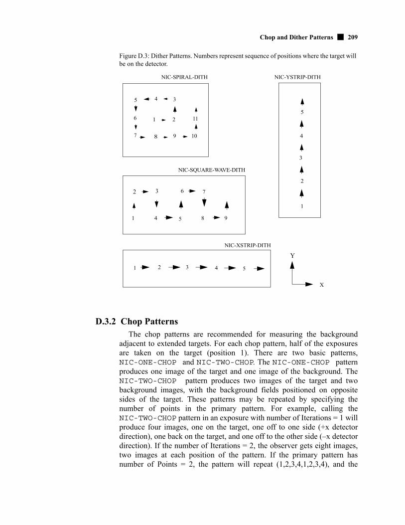
Chop and Dither Patterns 209
Figure D.3: Dither Patterns. Numbers represent sequence of positions where the target will be on the detector.
D.3.2 Chop PatternsThe chop patterns are recommended for measuring the background
adjacent to extended targets. For each chop pattern, half of the exposuresare taken on the target (position 1). There are two basic patterns,NIC-ONE-CHOP and NIC-TWO-CHOP. The NIC-ONE-CHOP patternproduces one image of the target and one image of the background. TheNIC-TWO-CHOP pattern produces two images of the target and twobackground images, with the background fields positioned on oppositesides of the target. These patterns may be repeated by specifying thenumber of points in the primary pattern. For example, calling theNIC-TWO-CHOP pattern in an exposure with number of Iterations = 1 willproduce four images, one on the target, one off to one side (+x detectordirection), one back on the target, and one off to the other side (–x detectordirection). If the number of Iterations = 2, the observer gets eight images,two images at each position of the pattern. If the primary pattern hasnumber of Points = 2, the pattern will repeat (1,2,3,4,1,2,3,4), and the
1 2
345
6
7 8 9 10
11
NIC-SPIRAL-DITH
NIC-SQUARE-WAVE-DITH
NIC-XSTRIP-DITH
NIC-YSTRIP-DITH
1
2 3
4 5
6 7
8 9
1 2 3 4 5
1
2
3
4
5
X
Y

210 Appendix D: Techniques for Dithering, Background Measurement and Mapping
observer will get eight images. Chop patterns are illustrated in Figure D.4,and the direction of the x- and y-axis are the same as in Figure 6.1.
Because chopping is best done to empty regions of the sky, we provide aset of chopping patterns that are in the CELESTIAL coordinate system, aswell as the standard set (that are in the POS-TARG frame). These have theword SKY in their name, and must have a pattern orientation angle (degreesE from N for the first motion of the pattern) supplied. These should be usedwhen the region around the target contains some objects that should beavoided when measuring the background. SKY patterns are illustrated inFigure D.6, and the direction of the x- and y-axis are the same as in Figure6.1.
Figure D.4: Chop Patterns.
D.3.3 Combined PatternsThe combined patterns permit dithering interleaved with chops to
measure the background. They are recommended for simultaneousminimization of detector artifacts and background subtraction, forobservations beyond 1.7 microns. Three types of combined patterns areimplemented: NIC-SPIRAL-DITH-CHOP,NIC-XSTRIP-DITH-CHOP, and NIC-YSTRIP-DITH-CHOP. Theircharacteristics are analogous to the dither patterns NIC-SPIRAL-DITH,NIC-XSTRIP-DITH, and NIC-YSTRIP-DITH, respectively, with theaddition that each dither step is coupled with a background image obtainedby chopping. These combined patterns are shown in Figure D.5, and thedirection of the x- and y-axis are the same as in Figure 6.1.
In a manner similar to the regular chop patterns, the combined patternshave “SKY” versions implemented in the CELESTIAL frame. The choppatterns require an pattern orientation angle which is defaulted to 0.0(North). The angle is measured from North through East. These areillustrated in Figure D.6.
1 2 1, 3 24
NIC-ONE-CHOP NIC-TWO-CHOP
X
Y

Chop and Dither Patterns 211
Figure D.5: Combined Patterns.
D.3.4 Map PatternsThere are two MAP sequences. These allow the telescope to be pointed
at a regular grid of points, doing a series of exposures at each point. Theseare done in the CELESTIAL frame, so a pattern orientation angle must besupplied, and the telescope motion on the sky is specified (rather than thetarget motion relative to the detector, see note above). TheNIC-SPIRAL-MAP sequence is basically the NIC-SPIRAL-DITHsequence in the CELESTIAL frame, and automatically maps the (square orrectangular) region around the target. The NIC-MAP sequence defines anarbitrary parallelogram on the sky. The observer may specify the number ofpoints in each of two directions, and the position angle (E of N) of eachdirection.
As with the dithering patterns, the observer has the option of specifyingwhether the target is centered in the pattern or not. The target will be
NIC-YSTRIP-DITH-CHOP
NIC-XSTRIP-DITH-CHOP
NIC-SPIRAL-DITH-CHOP
1 3
579
11
13 15
2 4
6810
12
14 16
CHOP-SIZEDITH-SIZE
1
2
3
4
5
6
7
8
9
10
11
12
13
DITH-SIZE
CHOP-SIZE
1 2
3 4
5 6
7 8
9 10
11 12
13
X
Y

212 Appendix D: Techniques for Dithering, Background Measurement and Mapping
centered in the NIC-SPIRAL-MAP pattern if there are 9, 25, 49,... pointsin the pattern, but will not necessarily be centered otherwise. The observercan specify if the target should be centered along one axis or the other, orboth, of the parallelogram defined by the sequence. These are illustrated inFigure D.6.
Figure D.6: Patterns on the sky. Numbers represent sequence of aperture pointings on the sky.
D.3.5 Combining Patterns and POS-TARGsOn occasion, it may be advantageous to specify a POS-TARG on the
exposure line to move the target to a different position than the aperturereference point. For this situation, the POS-TARG offset is alwaysperformed first to change the telescope pointing. For example, a user wantsto position a target in each of the four quadrants in Camera 2. The userspecifies the NIC2-FIX aperture for which the aperture reference point is atthe center of the array (128128 pixels) and specifies a POS-TARG–4.8,–4.8. A four point dither pattern using the NIC-SPIRAL-DITHpattern with point spacing = 9.6 arcseconds and pattern orient = 0 would
N
E
1
2
NIC-SKY-ONE-CHOP,ORIENT=210
1
2
4
NIC-SKY-TWO-CHOP,ORIENT=300
1
2
34
56
7
8
910
1112
NIC-XSTRIP-DITH-SKY-CHOP,ORIENT=110
1 2 3 4 5
6 7 8 9 10
11 12 13 14 15
1
2
3
4
5
6
7
8
9
1011
1213
14
1
2
3
4
5
6
7
NIC-SKY-SPIRAL-DITH-CHOP,ORIENT=260
NIC-SPIRAL-MAP,ORIENT=315
NIC-MAP, ORIENT1=335, ORIENT2=270
SPA
CIN
G1
SPACING2
CHOP-SIZE

Examples 213
achieve the desired results. (See the following example.) The target will bein the lower left quadrant of the array for the first position of the pattern,the lower right for the second position, the upper right for the thirdposition, and in the upper left quadrant for the fourth position of thepattern.
D.3.6 Generic PatternsPredefined convenience patterns are recommended for NICMOS
observations. These predefined patterns can be selected using the APTpattern editor. Observers can specify their own pattern by using a genericpattern form. Patterns are not supported by calnicb which combinesdithered observations into a mosaic. The IRAF/STSDAS task drizzle andMultiDrizzle (Koekemoer et al., 2002 HST Calibration Workshop, p337)can also be used to combine images into a mosaic. See also the newMultidrizzle Handbook (Fruchter et al 2009) for examples on how tocombine NICMOS data with Multidrizzle.
D.4 Examples
The next few pages show some selected examples of how the patternswork on astronomical observations.

214 Appendix D: Techniques for Dithering, Background Measurement and Mapping
Figure D.7: NIC-SKY-TWO-CHOP pattern.
#1
#4 #3
#2
Images Taken:
1 24Spacing (chop throw) = 1 detector width,Pattern Orient = 270°,Visit Orient = 225°,(Frame=CELESTIAL)
N
E
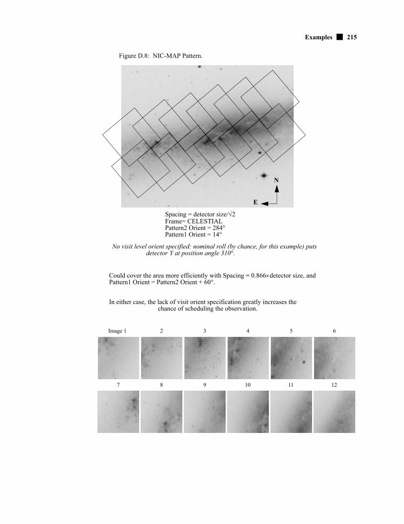
Examples 215
Figure D.8: NIC-MAP Pattern.
Spacing = detector size/2
No visit level orient specified: nominal roll (by chance, for this example) puts
Could cover the area more efficiently with Spacing = 0.866detector size, and Pattern1 Orient = Pattern2 Orient + 60°.
In either case, the lack of visit orient specification greatly increases the
Image 1 2 3 4 5 6
7 8 9 10 11 12
N
E
Frame= CELESTIALPattern2 Orient = 284°Pattern1 Orient = 14°
detector Y at position angle 310°.
chance of scheduling the observation.

216 Appendix D: Techniques for Dithering, Background Measurement and Mapping
D.5 Types of Motions
The Phase II optional parameter OFFSET defines which type oftelescope motion will be performed during a pattern. Telescope motionsfall into three categories:
• Small angle maneuvers (SAMs) where FGS Fine Lock guiding is maintained. Such SAMs are typically limited to < 2 arcmin from the point of the initial guide star acquisition. This is the practical limit of the radial extent of the pattern. Often it will be smaller due to guide star availability.
• SAMs without FGS guiding (i.e. GYRO pointing control). These are necessary for larger motions (> 2 arcmin). The telescope will drift at a rate of 1 to 2 milliarcsec per second of time (elapsed time since dropping to gyro—not exposure time).
• SAMs with RE-ACQuisitions of guide stars at each return to the tar-get position. This can be used to chop between a target and an offset background measurement pointing (which would be observed with GYRO pointing control).
The available options for OFFSET are:
• SAM, the default, will use guide stars whenever possible. If a motion, or the sequence of motions, moves the telescope sufficiently from the original position that guide stars are no longer available, then expo-sures will be obtained using GYRO control. If a subsequent motion returns the telescope to a point where the original guide stars become available then the guide stars will be RE-ACQuired. This incurs an overhead of ~3 minutes for each RE-ACQuisition.
The use of the Field Offset Mirror (FOM) to perform dithering andmapping is an “available” (not “supported”) mode of observation. TheFOM is not exactly repeatable, so artifacts on the mirror may appear tomove around. Observations requiring small and rapid offsets (or makingobservations in parallel to another instrument) may benefit from this mode.Note that the astigmatism changes with FOM offsets. Note: flat fieldcalibration reference files are only available for the nominal FOM position.

APPENDIX E:
The NICMOS CoolingSystemIn this chapter . . .
E.1 The NICMOS Cooling System
The purpose of the NICMOS Cooling System (NCS) is to enablecontinued operation of NICMOS by cooling the detectors to a scientificallyuseful temperature. This is achieved by a closed-loop circuit which runscryogenic gas through a coil inside the NICMOS dewar. The NCS providesexcellent temperature control, the detectors are maintained at77.15±0.10K. There is margin in the compressor speed to compensate forvariations in the parasitic heat load due to orbital and seasonal changes inspacecraft attitude as well as in the operation of the HST scienceinstruments in the aft shroud.
The NCS consists of three major subsystems: 1) a cryocooler whichprovides the mechanical cooling, 2) a Capillary Pumped Loop (CPL)which transports the heat dissipated by the cryocooler to an externalradiator, and 3) a circulator loop which transports heat from the inside ofthe NICMOS dewar to the cryocooler via a heat exchanger. Additionalelements of the NCS are the Power Conversion Electronics (PCE) whichprovides the up to 400 W of power needed by the cooler, and the ElectronicSupport Module (ESM) which contains a microprocessor to control theheat flow. Figure E.1 shows a schematic of the system.
E.1 The NICMOS Cooling System / 217
217

218 Appendix E: The NICMOS Cooling System
Figure E.1: Overview of the NCS.
In what follows, we give a more detailed description of the NCSsubsystems:
The cryocooler, manufactured by Creare, Inc., is a reverse-Braytoncycle turbine design. The compression and subsequent expansion of theNeon gas results in a net cooling which is used to remove heat from theNICMOS dewar via the heat exchanger to the circulator loop (see FigureE.1). The Creare design has several major advantages for application onHST. First, the closed loop system operates at very high speed—about7000 revolution per second—which limits the probability of mechanicalcoupling to the HST structure, thus minimizing the risk of spacecraft jitter.Second, the system is capable of providing large cooling power. Finally,the Creare design is compact enough to fit into the previously unused spacebetween the NICMOS enclosure and the HST aft end bulkhead.
On average, the cryocooler dissipates about 375 W of power whichneeds to be removed from the aft shroud. This is achieved via aAmmonia-filled Capillary Pumped Loop (CPL) that thermally connects thehousing of the compressor pump with an external radiator. The continuousheat flow through the (passive) CPL lines is maintained by a set of heatersthat are controlled by the ESM micro controller.
The heat from inside NICMOS is transported to the cryocooler via a setof flex lines. The flex lines connect to the inside of the dewar via bayonetfittings at an interface plate outside of the dewar which was accessible to
HST AFT SHROUD
NICMOS
Existing NICMOS Instrument
Astronaut AccessibleConnector
NICMOSCooling Loop
Flex Lines
Pump
Cryocooler
HeatExchanger
ExternalRadiator
Capillary Pumped Loop
Power
PowerConversionElectronics
Power
Control
Control
J600
HST EXTERNAL
μprocessorRemoteInterface
UnitThe World
Sensors
Sensors
Sensors
SpacecraftComputer
Aft Shroud Cooling SystemCapillary Pumped Loop Controls
and Sensors
Bayonet
Bayonet
Existing HST Spacecraft Equipment
HST Aft Shroud
New NICMOS Cryocooler Subsystem
New Microprocessor
New Radiator and CPL

The NICMOS Cooling System 219
the astronauts during SM3B. The circulator loop was then filled with Neongas from high pressure storage bottles. The bottles provide enough gas topurge, pressurize, and, if necessary, re-pressurize the circulator loop. TheNeon gas, driven by a high speed circulator pump and cooled via the heatexchanger to the cryocooler loop, circulates through the cooling coil at theaft end of the NICMOS dewar (see Figure E.2), thus cooling the entireinstrument.
The ESM uses the telemetry readings from the inlet and outlettemperature sensors at the NICMOS/NCS interface in an active control lawto regulate the cooling power of the NCS, and thus provide stability of theoperating temperature of the NICMOS detectors. Because of the sensitivedependence of a number of detector characteristics on temperature (seeChapter 7), the temperature stability is a crucial requirement on NCSperformance. To date, the stability has been extremely good with T=77.15with a variation of ~0.10K
All components of the NCS are combined into a common enclosure, theNICMOS Cryo Cooler (NCC). Figure E.2 shows a line drawing of theNCC, without any Multi-Layer Insulation (MLI). The system wassuccessfully tested in space during the HST Orbital Systems Test (HOST)shuttle mission in 1998. Remaining uncertainties about the NCSperformance stemmed from the natural lack of tests with the actualNICMOS dewar. This led to a longer than expected cooling time followingthe NCC installation, but has not affected the temperature stability.
Figure E.2: Line drawing of the NCC structure.

Glossary andAcronym List
The following terms and acronyms are used in this Handbook.
ACCUM: Accumulate readout mode for NICMOS observations.
ACS: Advanced Camera for Surveys.
ACQ: Observing mode in which the brightest source is located in asub-array and the telescope is repositioned to place the source behind thecoronagraphic hole.
A-D: Analog to digital.
ADC: Analog to digital converter.
ADU: Analog digital unit; 1 ADU = 1 DN.
ASCS: Aft Shroud Cooling System.
APT: The Astronomer’s Proposal Tool.
Breathing: Short term focus oscillations due to thermal variations on anorbital time scale.
BRIGHTOBJ: Bright object observing mode.
CALNICA: Primary NICMOS calibration task.
CALNICB: Secondary NICMOS calibration task used after CALNICA onthose exposures which comprise an association.
CCD: Charge-coupled device. Solid-state, light detecting device.
CDBS: Calibration Data Base System; system for maintaining referencefiles and tables used to calibrate HST observation datasets.
Chop: A spatial offset of up to 1440 arcsec of the aperture with respect tothe target, intended for the measurement of the background at one or morelocations significantly removed from the target pointing.
COS: Cosmic Origins Spectrograph.
221

222 Glossary and Acronym List
COSTAR: Corrective Optics Space Telescope Axial Replacement.
CP: Call for Proposals.
CPL: Capillary Pumped Loop.
CR: Cosmic Ray.
CVZ: Continuous Viewing Zone.
CP: Contact Scientist.
Dither: A small spatial offset (no more than 40 arcsec) of the position ofthe target in the aperture between successive observations.
DN: Data Number.
Drizzle: A technique (and STSDAS task) for the linear image reconstruc-tion of dithered images.
DSS: Digitized Sky Survey.
DQ: Data Quality.
DQE: Detector Quantum Efficiency.
ESM: Electronic Support Module.
ETC: Exposure Time Calculator.
FAQ: Frequently Asked Questions.
FDA: Field Divider Assembly.
FET: Field Effect Transistor.
FGS: Fine Guidance Sensors.
FITS: Flexible Image Transport System. A generic IEEE- andNASA-defined standard used for storing image data.
FOC: Faint Object Camera.
FOM: Field Offset Mirror (or mechanism).
FOS: Faint Object Spectrograph.
FOV: Field Of View.
FPA: Focal Plane Array.
FSW: Flight Software.
FTP: File Transfer Protocol; basic tool used to retrieve files from a remote system.
FWHM: Full Width at Half Maximum.
GHRS: Goddard High Resolution Spectrograph.
GO: General Observer.
GS: Guide Star.
GSC: Guide Star Catalog.
GSFC: Goddard Space Flight Center.
Glossary and Acronym List 223
GTO: Guaranteed Time Observer.
HOST: HST Orbital Systems Test.
HSP: High Speed Photometer.
HST: Hubble Space Telescope.
ICD: Interface Control Document; defines data structures used betweensoftware or systems to ensure compatibility.
IDT: Instrument Development Team.
IR: Infrared.
IRAF: Image reduction and analysis system. The system on which STS-DAS is built.
IRAS: Infrared Astronomical Satellite.
ISR: Instrument Science Report.
Jansky: The standard flux unit for NICMOS documentation and software.1 Jy = 1.0 10-26 W/m2/Hz = 1.0 10-23 erg/s/cm2/Hz.
Jy: Jansky.
K: Degrees Kelvin.
LSF: Line Spread Function.
MLI: Multi-Layer Insulation.
MOS: Multi-Object Spectroscopy.
Mosaic: A single image produced by combining the multiple images con-tained in a NICMOS associated data set; this combination is done by theSTSDAS task calnicb.
MULTIACCUM: Multiple-accumulate readout mode for NICMOS obser-vations.
MultiDrizzle: Automates and simplifies the detection of cosmic rays andthe combination of dithered observations using the Python scripting lan-guage and PyRAF (Koekemoer et al., 2002 HST Calibration Workshop,p337).
NCC: NICMOS CryoCooler.
NCS: Nicmos Cooling System.
NICMOS: Near-Infrared Camera and Multi-Object Spectrometer.
NIR: Near Infrared.
NUV: Near ultraviolet.
OPUS: OSS and PODPS Unified Systems.
OSS: Observation Support System.
OTA: Optical Telescope Assembly.
OTFR: On-The-Fly Reprocessing.

224 Glossary and Acronym List
PACOR: Packet process.
POD: Packetized Observation Data.
PAM: Pupil Alignment Mirror (or mechanism).
PC: Program Coordinator.
PCE: Power Conversion Electronics.
PED: Proposal editor.
Phase I: The process of submitting a proposal for HST observations.
Phase II: The process of designing accepted HST observing proposals.
PI: Principal Investigator.
PODPS: Post-Observation Data Processing System.
PSF: Point Spread Function.
QE: Quantum Efficiency.
RA: Right Ascension.
RMS: Root Mean Square.
RTO: Reuse Target Offset.
SAA: South Atlantic Anomaly.
SAM: Small Angle Maneuver.
SAMP-SEQ: Pre-defined sample sequence (readout times) for NICMOSobservations.
SLTV: System Level Thermal Vacuum (testing phase).
SM: Servicing mission.
SMOV: Servicing Mission Orbital Verification.
S/N: Signal-to-Noise ratio. Also seen as SNR.
SSR: Solid State Recorder.
STAN: Space Telescope Analysis Newsletter.
StarView: The user interface to the HST data archive.
ST-ECF: Space Telescope European Coordinating Facility.
STIS: Space Telescope Imaging Spectrograph.
STScI: Space Telescope Science Institute.
STSDAS: Space Telescope Science Data Analysis System. The completesuite of data analysis and calibration routines used to process HST data.
TAC: Telescope Allocation Committee.
TEC: Thermal Electrically Cooled shells.
TinyTim: Program which produces simulated HST point spread functions.
URL: Uniform resource locator; address for WWW.
UV: Ultraviolet.

Glossary and Acronym List 225
VCS: Vapor Cooled Shield.
WFPC: Wide Field/Planetary Camera.
WFPC2: Wide Field Planetary Camera 2; replacement for WF/PC installedduring first servicing mission of December 1993.
WWW: World Wide Web; hypertext-oriented method for finding andretrieving information over the Internet.
YSO: Young Stellar Object.

Index
A
ACCUM 13dark current calibration 130function of 122minimum time 128mode, described 24, 128multiple reads 128
accumulate modesee "ACCUM"
ACQ 25, 27, 71, 73function of 122mode, described 132
active control law 219afterimages 60amplifier glow 106, 130
described 116non-linearity 116
aperturedefining 99NIC1 through NIC3-FIX 100NIC2-ACQ 72NIC2-CORON 71, 72
arraycomparison to CCD 26read 123reset 123
artifactsamplifier glow 106, 116, 130shading 114
associations 203atomic lines 189attached parallel 27
B
background 9, 15ground-based 62infrared 62radiation 93
in exposure calculations 136spectroscopy 93thermal 62, 106, 136, 147zodiacal 62, 136zodiacal light 62
bad pixels 104, 118, 203detector 106
bandpasssee "filter"
Becklin-Neugebauer object 45bleeding 26breathing 58bright object limitations 60bright object mode
see "BRIGHTOBJ"bright targets 74BRIGHTOBJ 25
calibration of mode 12exposure times 198function of 122mode, described 197
C
cameraattached parallel 27changing, overhead 145field of view 22filters 33focus 50
227

228 Index
image quality 50orientation 23resolution 22spatial resolution
NIC1 22NIC2 23NIC3 23
spectroscopy, camera 3 89camera 1 through camera 3
see "camera" and "filter"CCD
compared to NICMOS array 26CELESTIAL 207, 210chop 202, 203
overhead 145patterns
ONE-CHOP 209TWO-CHOP 209
CO lines 189cold baffling 69cold pixels 118combined patterns
SPIRAL-DITH-CHOP 210XSTRIP-DITH-CHOP 210YSTRIP-DITH-CHOP 210
continuous viewing zone 66conversion tool 179cooling system 1, 217
capillary pumped loop 218circulator loop 217, 218, 219circulator pump 219compressor pump 218cooling coil 219cryocooler 219electronic support module 218flex lines 218heat exchanger 217, 218, 219multi-layer insulation 219NCS 1, 8, 18, 20, 219power conversion electronics 217
coordinate systemNICMOS 100, 101
coronagraphy 15aperture 100cold mask 16
coronagraphic hole 10, 71coronagraphic mask 23image contrast, PSF centering 76observations 11, 12occulting spot 16target acquisition 132
overhead 144cosmic rays 10, 59, 60
effect 59CPL (Capillary Pumped Loop)
see "cooling system"cryocooler
see "cooling system"CVZ
see "continuous viewing zone"
D
dark current 106calibration in ACCUM or MULTIACCUM
130detector 24, 106exposure times 131
datadata negative limit 73readout, overhead 145
DEFOCUSmode 12, 49
detectoramplifier glow 106, 116, 130array reset 123arrays 111artifacts 114bad pixels 106bias 123bright object limitations 25characteristics 105dark current 24, 106, 130described 24DQE 106dynamic range 24, 106, 112gain 105HgCdTe 24, 104linearity 106, 112non-destructive read 26non-linearity 24

Index 229
operations 24photovoltaic 103quantum efficiency 106read noise 24, 106, 111readout modes 24, 121response 106, 112saturation 106, 112shading
see "shading"throughput 42well depth 106
dewar 19, 21, 217, 218aft end 20cold mask 57
shifts 58cryogenic liquid 217inner shell 18solid nitrogen 20thermal short 8, 18
diffractionrings 57spikes 57
diffraction limited 22, 33dispersion direction 96dither 10, 202, 203
patterns 11SPIRAL-DITH 208SQUARE-WAVE-DITH 208XSTRIP-DITH 208YSTRIP-DITH 208
dynamic rangedetector 106
E
earthshine 66electronic bars 117emission lines
exposure times 136emissivity 64encircled energy 9, 55epsilon diagrams 93ESM (Electronic Support Module)
see "cooling system"exclusion
F164N, camera 3 173
F175W, camera 3 174F187N, camera 3 175F190N, camera 3 175F196N, camera 3 176F200N, camera 3 176F212N, camera 3 177F215N, camera 3 177F222M, camera 3 178F240M, camera 3 178grisms 93polarizers 83
exposure time calculatorextended objects 133point sources 133signal-to-noise 134
exposure timesbackground radiation 135BRIGHTOBJ 198calculating 138dark current 131emission line contribution 136instrument parameters 138instrumental factors 135signal-to-noise, calculating 136
F
F090M through F237Msee "filter"
FETsee "field effect transistor"
FGS (Fine Guidance Sensors) 23field effect transistor 104field of view
cameras 22field offset mirror
optical path 21parallel observation 216PSF 58
filter 33available, list of 33bandpasses 36, 38, 40camera 1 35camera 2 37camera 3 39described 22, 33

230 Index
F090M, camera 1 154F095N, camera 1 154F097N, camera 1 155F108N, camera 1 155F108N, camera 3 171F110M, camera 1 156F110W, camera 1 156F110W, camera 3 171F113N, camera 1 157F113N, camera 3 172F11W, camera 2 162F140W, camera 1 157F145M, camera 1 158F150W, camera 3 172F160W, camera 1 158F160W, camera 2 163F160W, camera 3 173F164N, camera 1 159F164N, camera 3 173F165M, camera 1 159F165M, camera 2 163F166N, camera 1 160F170M, camera 1 160F171M, camera 2 164F175W, camera3 174F180M, camera 2 164F187N, camera 1 161F187N, camera 2 165F187N, camera 3 175F187W, camera 2 165F190N, camera 1 161F190N, camera 2 166F190N, camera 3 175F196N, camera 3 176F200N, camera 3 176F204M, camera 2 166F205W, camera 2 167F207M, camera 2 167F212N, camera 2 168F212N, camera 3 177F215N, camera 2 168F215N, camera 3 177F216N, camera 2 169F222M, camera 2 169F222M, camera 3 178
F237M, camera 2 170F240M, camera 3 178filter wheel 33G141 95leak 34nomenclature 33polarimetry 83sensitivities 41sensitivity curves, polarizers 83sensitivity parameters 139–141spectroscopy 33, 93transmission 135
flat fieldcolor dependent 48response 108sensitivity variations 10
fluxJansky 3, 181magnitude systems 180standard stars 41unit conversion 181
examples 189units 3, 181
focuscamera 1 50camera 2 50history 48NIC3 18out-of-focus operations 55pupil alignment mechanism 48
FOMsee "field offset mirror"
FOS (Faint Object Spectrograph) 19
G
gain see "detector"
ghosts 60glint 70, 78glow
amplifier, see "amplifier glow"grisms 10, 23
available 39background radiation 136described 89

Index 231
resolving power 16spectroscopy 15, 89
grot 118guide star
acquisition overhead 144reacquisition overhead 144
H
helium lines 189Help Desk
contacting 6history 7HOST (HST Orbital Systems Test) 219hot pixels 118hydrogen lines 189
I
IDT "Instrument Development Team" iximage
quality 50strehl ratios 50
imagingfilters 33infrared 15polarimetry 15sensitivity limits 15
instrument 100camera orientation 23coordinate system 100design 19field divider 22field of view 22field offset mirror 21filters 3ƒ ratio 22optical train 22, 48optics 21overview 19pixel size 22pupil alignment mechanism 21setup time, overhead 144
intrapixel sensitivity 44
J
Jansky 3see also "flux"
jitter 218
L
leaksfilters 34
linearity 112detector 106
linesatomic 189molecular 189
LOW-SKY 66
M
magnitudeCIT system 182flux conversion 181infrared system 180UKIRT system 182zero points 182
map patternsSPIRAL-MAP 211
mapping 203MLI (Multi-Layer Insulation)
see "cooling system"modes 26
ACCUM 122, 128ACQ 27, 122BRIGHTOBJ 122detector readout 24INT-ACQ 27, 75mode-2 acquisition 72, 132MULTIACCUM 121, 122, 123
molecular lines 189mosaic 202MULTIACCUM 10, 12, 13, 25
dark current calibration 130dynamic range 124function of 122mode, described 24, 122, 123SAMP-TIME 123

232 Index
multiple accumulate modesee "MULTIACCUM"
multiple initial and final reads 128, 137
N
NCC (NICMOS Cryo Cooler) see "cooling system"
NCS (NICMOS Cooling System) see "cooling system"
NEXP 206NIC1 8, 9, 12, 50
encircled energy 51optimal focus 50
NIC1 through NIC3-FIXsee "aperture" 100
NIC2 8, 9, 12, 50encircled energy 51
NIC3 8, 9, 12best focus 54vignetting 56
NICMOS cooling system see "cooling system"
NICMOS cryocooler see "cooling system"
NICMOS-ORIENT 101NIC-SPIRAL-DITH 207non-destructive readout 123, 124, 128NREAD 128NSAMP 123, 124Nyquist sampling 57
O
observationattached parallel 27coronagraphic, planning 79grism, planning 96planning 29polarimetry, planning 87
observing patternspredesigned 207
NIC-MAP 207NIC-ONE-CHOP 207NIC-ONE-SKY-CHOP 207NIC-SPIRAL-DITH 207
NIC-SPIRAL-DITH-CHOP 207NIC-SPIRAL-DITH-SKY-CHOP 207NIC-SPIRAL-MAP 207NIC-SQUARE-WAVE-DITH 207NIC-TWO-CHOP 207NIC-TWO-SKY-CHOP 207NIC-XSTRIP-DITH 207NIC-XSTRIP-DITH-CHOP 207NIC-XSTRIP-DITH-SKY-CHOP 207NIC-YSTRIP-DITH 207NIC-YSTRIP-DITH-CHOP 207
OFFSET 216on-board acquisition 27operating mode
overheads 144optical baffles 118optical elements
grisms 89optical telescope assembly
breathing 58optics
astigmatism 57coma 57dewar 21elements 33emissivity 64filters 33grisms 39
orbitsrequired, calculating 147time requests 143
ORIENT 101orientation
described 101OTA
see "optical telescope assembly"overhead 143
coronagraphy 147example, polarimetry 147examples 147instrument specific 144NICMOS specific 144observatory level 144

Index 233
P
paint flakes see "grot"
PAM 48see "pupil alignment mechanism"
parallelsattached 27
pattern parameter form 202PCE (Power Conversion Electronics)
see "cooling system"pedestal 66persistence 26
cosmic ray 10, 60, 78, 134photon 10, 60
photodiode 104photometric stability 42photometry
Johnson’s system 180red source 45sources with extreme colors 45stability 42Vega 180young stellar objects 45
plate scale 15, 16, 22pointing
HST 11polarimetry 15
example 147filters 33spectral coverage 33
polarizers 23POS-TARG 99, 100, 203, 206, 207, 210post-SAA 61proposal
instructions 6overheads, exposure 144Phase I 2Phase II 2Phase II Proposal Instructions 2submission process 6unsupported modes 12
PSF 57, 137centering 76field dependence 58field offset mirror 58
NIC3 11Nyquist sampling 57subtraction 10temporal dependence 58temporal variations 76
pupil alignment mechanism 8, 18focus 48optical path 21
Q
qualityimage 50
R
re-acquisitions 144read noise
described 111detector 106
readoutACCUM mode 122, 128ACQ mode 122, 132BRIGHTOBJ
exposure times 198mode 122, 197
MULTIACCUM mode 122, 123, 130non-destructive 128NSAMP 124SAMP-TIME 123
readout modesdetector 24
resolutioncameras 22
re-use target acquisitiondescribed 26
reuse target offset 27, 75, 77, 79RT ANALYSIS 75RTO
see "reuse target offset"
S
SAAsee "South Atlantic Anomaly"
SAMsee "small angle maneuvers" 99

234 Index
SAMP-TIME 123saturation
detector 106sensitivity
F164N, camera 3 173F171M, camera 2 164F175W, camera 3 174F187N, camera 3 175F190N, camera 3 175F196N, camera 3 176F200N, camera 3 176F212N, camera 3 177F215N, camera 3 177F222M, camera 3 178F237M, camera 2 170F240M, camera 3 178grisms 93limits 15polarizers 83
servicing missionSM3B 1, 20, 219
shading 26, 74, 106, 114dark current removal 130described 26, 114
shutterdetector reset 123
shutter mechanism 123signal-to-noise 133
calculating 136sky brightness
zodiacal background 62small angle maneuvers 99, 145, 216software
spectroscopy reduction 96South Atlantic Anomaly 60Space Telescope European Coordinating Facil-
ity (ST-ECF) 7spacecraft jitter 218spacecraft orientations 101spectroscopy 15
central wavelength 89complex fields 96dispersion 96G141 95grism, general 15
grisms, described 89sensitivity 93spectral coverage 89
STSDAScalibration 48
T
target acquisition 26ACQ mode, described 26aperture 99, 100interactive 26onboard 26, 132re-use target offset 26
target acquisition mode 24TECs
see "thermally electrically cooled shells"telescope
motion 99motion, overhead 144small angle maneuvers 99
thermal background 62, 94, 136, 202thermal electrically cooled shells 19thermal emission 64, 110thermal regime 9thermal short
see "dewar"thermal stress 57throughput 15time-resolved images 25TinyTim 55TWO-CHOP 147
U
unitsin Handbook 3microns 3
user supportHelp Desk 6
V
vapor cooled shield 19Vega 180

Index 235
vignetting 54cameras 1 and 2 54cold 56NIC3 56warm 56
Visual Target Tuner (VTT) 32
W
wavefront error 56wavelength
units 3World Wide Web
NICMOS Web page 7
Y
young stellar objects (YSOs) 45, 47
Z
zodiacal background 62, 136

236 Index