NBIS-Metagenomics DocumentationRelease 1.0

John Sundh

May 08, 2020

Setup

1 Installation 1

2 Quick start guide 3

3 General configuration settings 5

4 The sample list file 7

5 How to run on UppMax/Hebbe (SNIC resources) 9

6 Preprocessing reads 11

7 Classify reads 15

8 Filtering results 17

9 Reference based mapping 21

10 Assembly 23

11 Annotation of coding sequences 25

12 Generating required database files 27

13 Binning metagenomic contigs 29

14 Overview 31

15 Installation 33

i

ii

CHAPTER 1

Installation

1. Clone the repository Checkout the latest version of this repository:

git clone https://bitbucket.org/scilifelab-lts/nbis-meta

Change directory:

cd nbis-meta

2. Install the required software All the software needed to run this workflow is included as a Conda environmentfile. To create the environment nbis-meta use the supplied envs/environment.yaml file.

First create the environment using the supplied file:

mkdir envs/nbis-metaconda env create -f envs/environment.yaml -p envs/nbis-meta

Next, add this directory to the envs_dirs in your conda config (this is to simplify activation of the environment and sothat the full path of the environment installation isn’t shown in your bash prompt):

conda config --add envs_dirs $(pwd)/envs/

Activate the environment using:

conda activate envs/nbis-meta

You are now ready to start using the workflow!

1

NBIS-Metagenomics Documentation, Release 1.0

2 Chapter 1. Installation

CHAPTER 2

Quick start guide

2.1 Using the examples

The workflow comes with a set of example datasets found in the examples/data folder. By default the workflowuses the configuration specified in the config.yaml file to do preprocessing and assembly of the example data.

To see what the workflow is configured to do in the default setup run:

snakemake -np

This performs a ‘dry run’ (specified by the -n flag) where nothing is actually executed just printed to the terminal.Try it out by removing the -n.

To familiarize yourself with ways to run the workflow you can make use of the example directories found underexamples/.

For instance, to run the centrifuge example (Read classification and taxonomic profiling using Centrifuge) do:

snakemake --configfile examples/centrifuge/config.yaml

See more about the examples here: binning, centrifuge, reference-based mapping

2.2 Using your own data

1. Create your sample_list

2. Configure the workflow to your needs. Make sure to updated the sample_list: path in the config.

Note: We recommend that you copy the config.yaml file to some other file, e.g. ‘myconfig.yaml’, and make yourchanges in the copy.

You are now ready to start the workflow using:

3

NBIS-Metagenomics Documentation, Release 1.0

snakemake --configfile myconfig.yaml

You can have multiple configuration files (e.g. if you want to run the workflow on different sets of samples or withdifferent parameters).

4 Chapter 2. Quick start guide

CHAPTER 3

General configuration settings

Here you’ll find information on how to configure the pipeline.

The file config.yaml contains all the parameters for the pipeline. The most general settings are explained here.For more specific settings regarding the different workflow steps you may refer to the corresponding documentation.

Note: The only required config setting is sample_list:. Without this, the workflow cannot run but essentiallyyour config file may contain only this parameter.

workdir: Working directory for the snakemake run. All paths are evaluated relative to this directory.

sample_list: should point to a file with information about samples. See the documentation on The sample listfile for more details on the format of this file.

taxdb: Path to where taxonomic database files from NCBI are stored.

results_path: this directory will contain reports, figures, count tables and other types of aggregated and pro-cessed data. Output from the different steps will be created in sub-directories. For instance, assemblies will be in asub-directory called ‘assembly’

intermediate_path: this directory contains files which might have required a substantial computational effort togenerate and which might be useful for further analysis. They are not deleted by Snakemake once used by downstreamrules. This could be for example bam files.

temp_path: this directory contains files which are either easily regenerated or redundant. This could be for examplesam files which are later compressed to bam.

scratch_path: Similar to temp_path but primarily used on cluster resources (e.g. Uppmax) in order to speed upwrites to disk by utilizing local storage for nodes.

resource_path: Path to store database files needed for the workflow.

report_path: Path to store report files such as assembly and mapping stats and plots

5

NBIS-Metagenomics Documentation, Release 1.0

6 Chapter 3. General configuration settings

CHAPTER 4

The sample list file

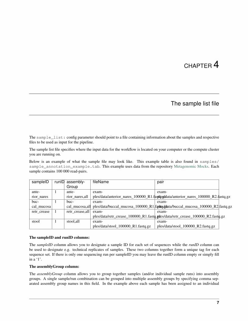
The sample_list: config parameter should point to a file containing information about the samples and respectivefiles to be used as input for the pipeline.

The sample list file specifies where the input data for the workflow is located on your computer or the compute clusteryou are running on.

Below is an example of what the sample file may look like. This example table is also found in samples/sample_annotation_example.tab. This example uses data from the repository Metagenomic Mocks. Eachsample contains 100 000 read-pairs.

sampleID runID assembly-Group

fileName pair

ante-rior_nares

1 ante-rior_nares,all

exam-ples/data/anterior_nares_100000_R1.fastq.gz

exam-ples/data/anterior_nares_100000_R2.fastq.gz

buc-cal_mucosa

1 buc-cal_mucosa,all

exam-ples/data/buccal_mucosa_100000_R1.fastq.gz

exam-ples/data/buccal_mucosa_100000_R2.fastq.gz

retr_crease 1 retr_crease,all exam-ples/data/retr_crease_100000_R1.fastq.gz

exam-ples/data/retr_crease_100000_R2.fastq.gz

stool 1 stool,all exam-ples/data/stool_100000_R1.fastq.gz

exam-ples/data/stool_100000_R2.fastq.gz

The sampleID and runID columns:

The sampleID column allows you to designate a sample ID for each set of sequences while the runID column canbe used to designate e.g. technical replicates of samples. These two columns together form a unique tag for eachsequence set. If there is only one sequencing run per sampleID you may leave the runID column empty or simply fillin a ‘1’.

The assemblyGroup column:

The assemblyGroup column allows you to group together samples (and/or individual sample runs) into assemblygroups. A single sample/run combination can be grouped into multiple assembly groups by specifying comma sep-arated assembly group names in this field. In the example above each sample has been assigned to an individual

7

NBIS-Metagenomics Documentation, Release 1.0

assembly as well as a co-assembly named ‘all’ which will contain all samples. Running the workflow with this filewill produce five assemblies in total (named ‘anterior_nares’, ‘buccal_mucosa’, ‘retr_crease’, ‘stool’ and ‘all).

The fileName and pair columns:

These two columns specify file paths for sequences in the (gzipped) fastq format. For paired end data the fileNamecolumn points to forward read file and the pair column points to the corresponding reverse read file. For single enddata only the fileName column is used.

8 Chapter 4. The sample list file

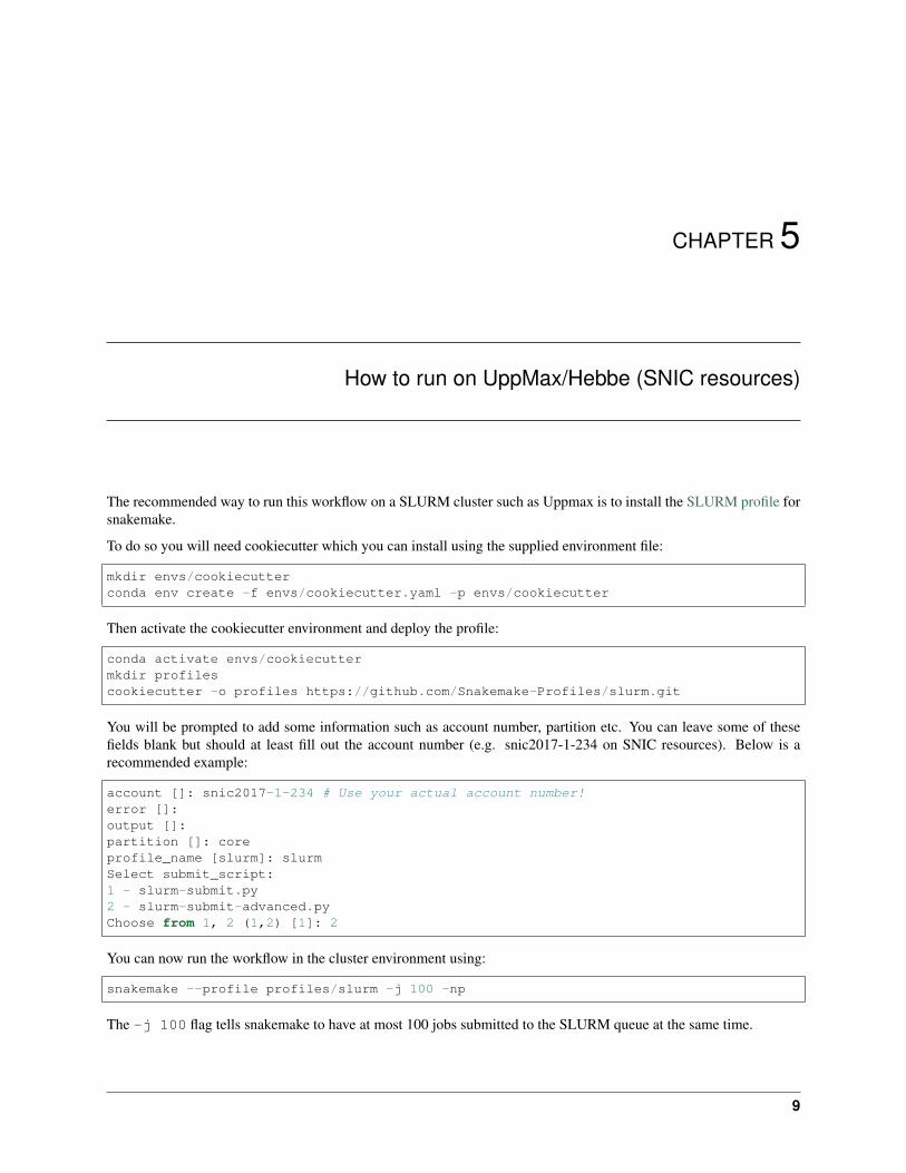
CHAPTER 5

How to run on UppMax/Hebbe (SNIC resources)

The recommended way to run this workflow on a SLURM cluster such as Uppmax is to install the SLURM profile forsnakemake.

To do so you will need cookiecutter which you can install using the supplied environment file:

mkdir envs/cookiecutterconda env create -f envs/cookiecutter.yaml -p envs/cookiecutter

Then activate the cookiecutter environment and deploy the profile:

conda activate envs/cookiecuttermkdir profilescookiecutter -o profiles https://github.com/Snakemake-Profiles/slurm.git

You will be prompted to add some information such as account number, partition etc. You can leave some of thesefields blank but should at least fill out the account number (e.g. snic2017-1-234 on SNIC resources). Below is arecommended example:

account []: snic2017-1-234 # Use your actual account number!error []:output []:partition []: coreprofile_name [slurm]: slurmSelect submit_script:1 - slurm-submit.py2 - slurm-submit-advanced.pyChoose from 1, 2 (1,2) [1]: 2

You can now run the workflow in the cluster environment using:

snakemake --profile profiles/slurm -j 100 -np

The -j 100 flag tells snakemake to have at most 100 jobs submitted to the SLURM queue at the same time.

9

NBIS-Metagenomics Documentation, Release 1.0

10 Chapter 5. How to run on UppMax/Hebbe (SNIC resources)

CHAPTER 6

Preprocessing reads

Read preprocessing can be run as a single part of the workflow using the command:

snakemake --configfile <yourconfigfile> preprocess

Input reads can be trimmed using either Trimmomatic or Cutadapt.

6.1 Trimmomatic

The settings specific to Trimmomatic are:

trimmomatic: Set to True to preprocess reads using Trimmomatic.

trimmomatic_home: The directory where Trimmomatic stores the .jar file and adapter sequences. If you don’tknow it leave it blank to let the pipeline attempt to locate it.

trim_adapters: Set to ‘True’ to perform adapter trimming.

pe_adapter_params: The adapter trim settings for paired end reads. This is what follows the ‘ILLUMINACLIP’flag. The default “2:30:15” will look for seeds with a maximum of 2 mismatches, and clip if extended seeds reach ascore of 30 for paired-end reads or 10.

pe_pre_adapter_params: Trim settings to be performed prior to adapter trimming. See the Trimmomaticmanual for possible settings. As an example, to trim the first 10 bp from the start of reads set this to HEADCROP:10.

pe_post_adapter_params: Trim settings to be performed after adapter trimming. To for instance set a 50 bpthreshold on the minimum lenghts of reads after all trimming is done, set this to MINLEN:50.

The se_adapter_params: and se_post_adapter_params: settings are the same as above but for single-end reads.

6.2 Cutadapt

cutadapt: Set to True to run preprocessing with cutadapt.

11

NBIS-Metagenomics Documentation, Release 1.0

Note: Trimmomatic has priority in the preprocessing so if both Trimmomatic and Cutadapt are set to True, onlyTrimmomatic will be run.

adapter_sequence: Adapter sequence for trimming. By default the workflow uses the Illumina TruSeq UniversalAdapter.

rev_adapter_sequence: 3’ adapter to be removed from second read in a pair.

cutadapt_error_rate: Maximum allowed error rate as value between 0 and 1. Defaults to 0.1. Increasing thisvalue removes more adapters.

6.3 Phix filtering

phix_filter: Set to True to filter out sequences mapping to the PhiX genome.

6.4 Fastuniq

fastuniq: Set to True to run de-duplication of paired reads using Fastuniq.

Note: Fastuniq only runs with paired-end reads so if your data contains single-end samples the sequences will just bepropagated downstream without Fastuniq processing.

6.5 SortMeRNA

SortMeRNA finds rRNA reads by aligning to several rRNA databases. It can output aligning, rRNA, reads and non-aligning, non_rRNA, reads to different output files allowing you to filter your sequences.

sortmerna: Set to True to filter your raw reads with SortMeRNA.

sortmerna_keep: Sortmerna produces files with reads aligning to rRNA (‘rRNA’ extension) and not aligning torRNA (‘non_rRNA’) extension. With the sortmerna_keep setting you specify which set of sequences you want touse for downstream analyses (‘non_rRNA’ or ‘rRNA’)

sortmerna_remove_filtered: Set to True to remove the filtered reads (i.e. the reads NOT specified in ‘keep:’)

sortmerna_dbs: Databases to use for rRNA filtering. Can include:

• rfam-5s-database-id98.fasta

• rfam-5.8s-database-id98.fasta

• silva-arc-16s-id95.fasta

• silva-arc-23s-id98.fasta

• silva-bac-16s-id90.fasta

• silva-bac-23s-id98.fasta

• silva-euk-18s-id95.fasta

• silva-euk-28s-id98.fasta

12 Chapter 6. Preprocessing reads

NBIS-Metagenomics Documentation, Release 1.0

sortmerna_paired_strategy: How to handle read-pairs where mates are classified differently. If set topaired_in both reads in a pair are put into the ‘rRNA’ bin if one of them aligns (i.e. more strict) whilepaired_out puts both reads in the ‘other’ bin.

sortmerna_params: Extra parameters to use for the sortmerna step.

6.6 Markduplicates

This is technically post-processing but to remove duplicates prior to producing read counts of ORFs called on assem-bled contigs you can set markduplicates:True. The picard_jar and picard_path can most often be leftblank as the workflow will automatically identify these paths in your conda environment. However, if you run intotrouble with this step try searching for picard.jar and its directory.

6.6. Markduplicates 13

NBIS-Metagenomics Documentation, Release 1.0

14 Chapter 6. Preprocessing reads

CHAPTER 7

Classify reads

Reads can be classified taxonomically using k-mer based methods. Two popular programs for this purpose are Cen-trifuge and Kraken2. The workflow can run both tools on all samples specified in your sample annotation file andproduce interactive krona-plots and kraken-style reports.

Database construction for kraken and centrifuge is not part of this workflow. Please refer to the respective documenta-tion for these tools (Kraken manual, Centrifuge manual). However, both tools have pre-built indices which saves youthe trouble of downloading and building these on your own.

Individual krona plots are created in results/centrifuge/ and results/kraken/. Combined krona plots are created inresults/report/centrifuge and results/report/kraken. The kraken-style *.kreport files created within these directoriescan be loaded into the tool pavian. Either install the pavian R package or run it using Docker (see instructions at theGitHub repo).

7.1 Centrifuge

Relevant settings for Centrifuge are:

centrifuge_prebuilt: By default, the workflow uses the prebuilt p+h+v index containing prokary-otic, viral and human sequences which it will download from the centrifuge FTP. Other valid choices are:p_compressed+h+v, p_compressed_2018_4_15, nt_2018_2_12 and nt_2018_3_3. The index willbe downloaded to resources/classify_db/centrifuge/.

centrifuge_custom: If you have created your own custom centrifuge index, specify the its path here, excludingthe .*.cf suffix.

centrifuge_summarize_rank: The centrifuge index can be summarized to see number of sequences and totalsize in bp for each taxa at a certain rank specified by this config parameter (superkingdom by default). To generate thesummary file run:

snakemake --config centrifuge=True centrifuge_summary

The summary output will be placed in the same directory as the centrifuge index (resources/classify_db/centrifuge ifusing the prebuilt index) in a file with the suffix ‘.summary.tab’.

15

NBIS-Metagenomics Documentation, Release 1.0

centrifuge_max_assignments: This determines how many assignments are made per read. By default thisparameter is set to 1 in this workflow which means centrifuge runs in ‘LCA’ mode similar to kraken where only thelowest common ancestor of all hits is assigned for a read. The default setting for centrifuge is 5.

centrifuge_min_score: This is used to filter out classifications when creating the kraken-style report. Notethat this also influences the numbers in the Krona plots.

You can try out the Centrifuge read classifier by using one of the supplied examples. To see the rules that would berun enter:

snakemake --configfile examples/centrifuge/config.yaml -np

Now perform the actual run with 4 cores:

snakemake --configfile examples/centrifuge/config.yaml -p -j 4

7.2 Kraken2

Relevant settings for Kraken2 are:

kraken_prebuilt: By default, the workflow uses the prebuilt MiniKraken2_v2_8GB database built fromthe Refseq bacteria, archaea, and viral libraries and the GRCh38 human genome. Alternatively you can useMiniKraken2_v1_8GB which will download the database excluding the human genome. These minikrakendatabases are downsampled versions of the standard database which could influence sensitivity. However, evalua-tions suggest that with kraken2 the drop in sensitivity is minimal.

kraken_custom: If you have created your own custom centrifuge index, specify the path to the directory containingthe hash.k2d, opts.k2d and taxo.k2d files.

kraken_reduce_memory: Set to True to run kraken2 with --memory-mapping which reduces RAM usage.

Try out the Kraken2 read classifier using the supplied example:

snakemake --configfile examples/kraken/config.yaml -np

16 Chapter 7. Classify reads

CHAPTER 8

Filtering results

Sometimes you may see taxa pop up in your classification output that you are not sure are really there. The k-merbased methods such as Centrifuge and Kraken do not provide information on e.g. genome coverage that tools likebowtie2 or blast can give. However, for very large datasets and very large genome databases using read-aligners is nottractable due to extremely long running times.

This workflow can utilize the speed and low disk-space requirements of Centrifuge to obtain a set of ‘trusted’ genomesthat are used for more detailed mapping analyses.

To try this out on the example above enter:

snakemake --configfile examples/centrifuge/config.yaml --config centrifuge_map_→˓filtered=True -np -j 4

Because we set centrifuge_map_filtered=True the output from Centrifuge is now filtered in a two-stepsetup.

To perform the actual runs (again with 4 cores) do:

snakemake --configfile examples/centrifuge/config.yaml --config centrifuge_map_→˓filtered=True -p -j 4

Below are explanations of the different filtering steps and the output produced.

8.1 Centrifuge filtering

First taxids with at least centrifuge_min_read_count assigned reads are identified and the correspondinggenome sequences are extracted from the Centrifuge database. By default centrifuge_min_read_count is setto 5000.

17

NBIS-Metagenomics Documentation, Release 1.0

8.2 Sourmash filtering

Next, genomes passing the first filter are passed to [sourmash](https://github.com/dib-lab/sourmash) which builds‘MinHash’ signatures of the genomes. These signatures are essentially highly compressed representations of the DNAsequences. Signatures are also computed for each (preprocessed) sample and these are then queried against the filteredgenome signatures. This gives an estimate of how much a genome is covered by a sample by comparing the MinHashsignatures. Settings which influence how this filtering step is performed are:

sourmash_fraction: the number of hashes to compute as a fraciton of the input k-mers. By default this is setto 100 meaning that 1/100 of the input k-mer are used to compute the MinHash signature. Increasing the setting willreduce the disk-space requirements but may also reduce performance.

sourmash_min_cov: This is the minimum coverage estimated from the sourmas filtering step that a genome musthave in order to pass to the next steps. By default this is set to 0.1 meaning that a genome must be covered by at least10%

in at least one of the samples.

8.3 Bowtie2 alignments

Finally, genomes that pass both filters are indexed using bowtie2 and the (preprocessed) reads are mapped to this setof genomes. The resulting bam-files are used to calculate coverage of genomes across samples.

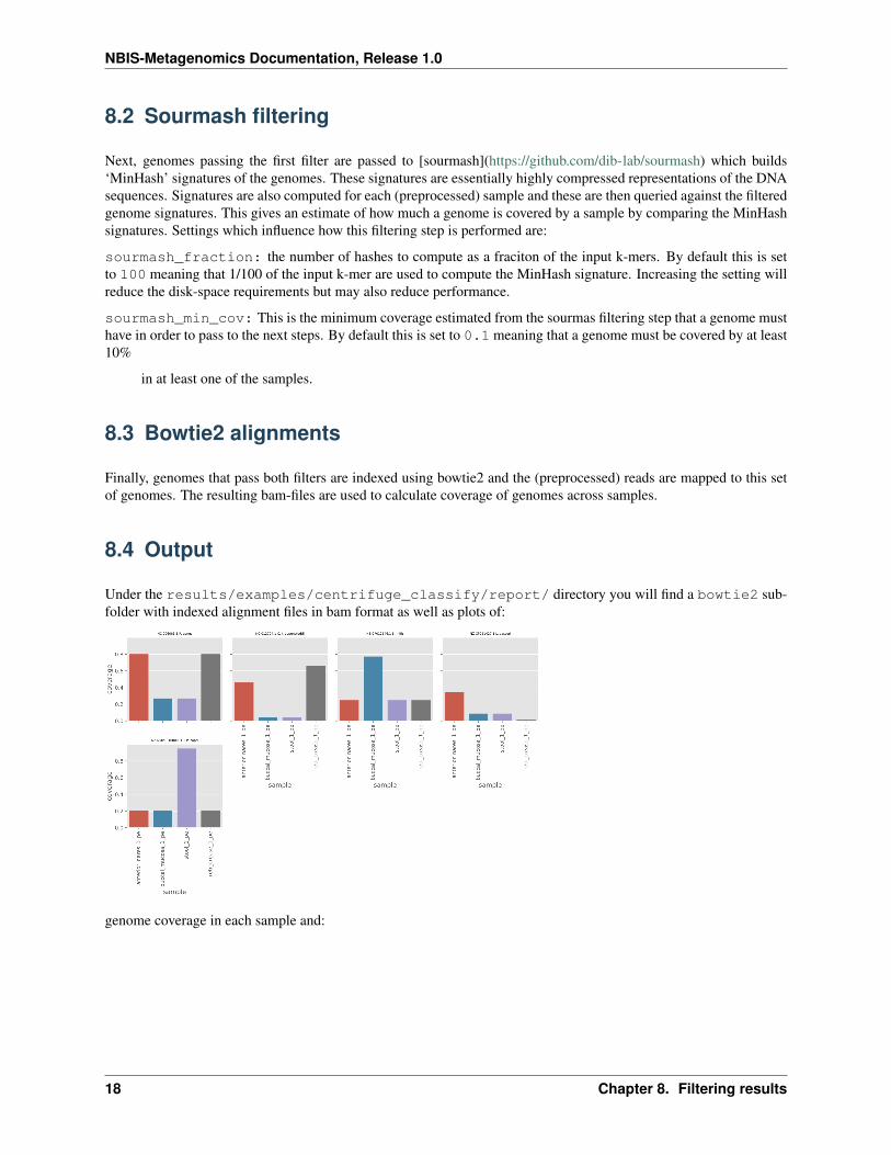
8.4 Output

Under the results/examples/centrifuge_classify/report/ directory you will find a bowtie2 sub-folder with indexed alignment files in bam format as well as plots of:

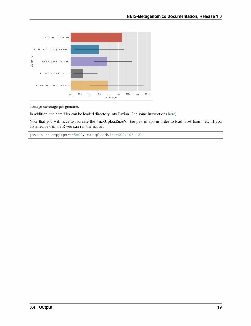
genome coverage in each sample and:

18 Chapter 8. Filtering results

NBIS-Metagenomics Documentation, Release 1.0

average coverage per genome.

In addition, the bam files can be loaded directory into Pavian. See some instructions here).

Note that you will have to increase the ‘maxUploadSize‘of the pavian app in order to load most bam files. If youinstalled pavian via R you can run the app as:

pavian::runApp(port=5000, maxUploadSize=500*1024^2)

8.4. Output 19

NBIS-Metagenomics Documentation, Release 1.0

20 Chapter 8. Filtering results

CHAPTER 9

Reference based mapping

This part of the workflow performs mapping of preprocessed reads against a set of reference sequences and reports onthe abundance of genomes and their coding sequences in your samples.

If you’re working with samples that you are fairly certain contain organisms with representative genome referencesthis type of analysis may suit you.

9.1 Prefiltering

The workflow will first use the read-based classifier Centrifuge to make a rough estimate of the genomes present inyour samples. The main advantage of this classifier is that the database doesn’t require a lot of storage (the full refseqdatabase of bacteria, archaea and viruses only takes up ~5 GB) so it’s good for doing a quick filtering run.

Take a look at How to configure the Centrifuge database) for more details.

The prefiltering step classifies all samples against the centrifuge database and filters out taxa that have at leastrefmap_min_read_count: mapped. The default is 50 reads but this can be changed in the config file or onthe command line by adding --config refmap_min_read_count <min_reads>.

Genomic data for genomes meeting the threshold in any of the samples is downloaded and a bowtie2 index is built.

9.2 Mapping

The workflow proceeds with mapping of reads against the set of filtered genomes using bowtie2. Read mappings arethen counted for each coding sequence defined in the reference GFF files that has a ‘protein_id’ in the attributes field.

9.3 Output

Raw counts and normalized abundances (TPM) of the coding sequences are reported for all samples as well as a fileof total genome coverage for the filtered genomes.

21

NBIS-Metagenomics Documentation, Release 1.0

PCA plots of samples based on raw and normalized coding sequence abundance as well as genome coverage are alsogenerated.

9.4 Example

To try out the reference based mapping you can use the example data under examples/data/ and the correspondingconfiguration file examples/refmap/config.yaml.

To speed up the building of the centrifuge database this example limits the organisms to include to a set of 28 taxonomyids specified in examples/refmap/taxids.

Simply run:

snakemake --configfile examples/refmap/config.yaml -p -j 4

to run the workflow with 4 cores (modify the -j parameter to change this).

22 Chapter 9. Reference based mapping

CHAPTER 10

Assembly

Assembly can be run as a single part of the workflow using the command:

snakemake --configfile <yourconfigfile> assembly

Megahit and Metaspades are currently the only assemblers supported by this workflow. Megahit is used by defaultso in order to use Metaspades you have to explicitly configure the workflow to do so (see below). Settings for theseassembler are:

assembly: Set to True to assemble samples based on the assemblyGroup column in your sample list.

assembly_threads: Number of threads to use for the assembly software.

megahit_keep_intermediate: If set to True, intermediate contigs produced using different k-mer lengths, aspart of the megahit assembly procedure, are stored. Note that this can take up a large chunk of disk space. By defaultthis is set to False.

megahit_additional_settings: The megahit assembler is run with default settings. Use this parameter toadd additional settings to the megahit assembler, such as ‘–preset meta-large’ or something else that you want tochange.

metaspades: Set to True to use the metaspades assembler instead of megahit

metaspades_keep_intermediate: As for megahit, setting this to True will store intermediate contigs createdduring assembly.

metaspades_keep_corrected: Set to True to keep corrected reads created during metaspades assembly.

metaspades_additional_settings: This is where you put any additional settings for metaspades.

10.1 Reports

The workflow produces a set of report files for the assemblies created. These files are saved in the directory specifiedby report_path: in your configuration file.

assembly_stats.pdf

23

NBIS-Metagenomics Documentation, Release 1.0

A multi-panel plot showing number of contigs, total assembly size, as well as various length statistics of each assemblycreated.

The figure below shows the plot for the example dataset.

24 Chapter 10. Assembly

CHAPTER 11

Annotation of coding sequences

This section deals with how to annotate protein sequences predicted on assembled contigs.

11.1 Protein family annotation

Annotation of predicted protein coding sequences is performed using the tools eggnog-mapper pfam_scan (using thelatest version of the PFAM database) and rgi (Resistance Gene Identifier).

eggnog: Set to True in order to annotate coding sequences with eggnog-mapper. This also adds annotations forKEGG orthologs, modules and pathways.

pfam: Set to True in order to add PFAM protein families to coding sequences.

rgi: Set to True in order to add AMR (Antimicrobial Resistance) gene families to coding sequences.

rgi_params: Determines how to run the rgi software. By default it’s run in ‘perfect’ mode, using the diamondalignment tool. See the rgi GitHub pages <https://github.com/arpcard/rgi#rgi-main-usage-for-genomes-genome-assemblies-metagenomic-contigs-or-proteomes>_ for more information.

Note: The eggnog-mapper, pfam_scan and rgi programs all utilize separate conda environments. In order to use thesetools you must run the workflow with the --use-conda flag.

11.2 Taxonomic annotation

Taxonomic annotation of protein sequences is performed by: 1. similarity searches against a reference database 2.parsing best hits for each protein query and linking hits to taxonomic IDs 3. assigning a taxonomic label to the lowestcommon taxa for the ‘best hits’

The first step above is performed in this workflow using Diamond against a protein sequence reference database. Theworkflow supports using the uniref50, uniref90, uniref100 or nr protein databases but you can also use a preformattedcustom database as long as it has been formatted with

25

NBIS-Metagenomics Documentation, Release 1.0

taxonomic_annotation: Set to True to add taxonomic annotations to contigs (and ORFs).

taxdb: Can be one of ‘nr’, ‘uniref50’, ‘uniref90’, ‘uniref100’ or you can add a custom diamond database if youformat it with taxonomic ids (using the –taxonmap and –taxonnodes flags to diamond makedb)

diamond_threads: How many threads to use for the diamond blast job.

taxonomy_min_len: Minimum length of contigs to be included in the taxonomic annotation.

tango_params: Additional parameters to use for the tango taxonomic assigner

taxonomy_ranks: Taxonomic ranks to use in output.

Note: If you want to use a custom preformatted protein database. Make sure to put it as ‘diamond.dmnd’ in the<resource_path> directory as specified in your configfile. Then run the workflow once with the -t flag to update thetimestamps on the existing files.

26 Chapter 11. Annotation of coding sequences

CHAPTER 12

Generating required database files

Several steps of this workflow requires large database files that may take a long time to download and format. If youwant to can run the database creation separately with the workflow (e.g. while you’re waiting for real data to arrive).

To create the databases needed for the protein annotation steps (eggnog, pfam, rgi and taxonomic) you can run:

snakemake --configfile config.yaml --config eggnog=True pfam=True rgi=True taxonomic_→˓annotation=True -np db

<lots of text>

Job counts:count jobs1 db1 db_done1 download_eggnog1 download_pfam1 download_pfam_info1 download_uniref1 get_eggnog_version1 get_kegg_ortholog_info1 prepare_diamond_db_uniref1 prepare_taxfiles_uniref1 press_pfam11

Note: The ‘db’ target only includes database files used in preprocessing (SortMeRNA) and protein annotation.

See also:

See the documentation for ways to create databases for read-classification.

27

NBIS-Metagenomics Documentation, Release 1.0

28 Chapter 12. Generating required database files

CHAPTER 13

Binning metagenomic contigs

Assembled contigs can be grouped into so called ‘genome bins’ using information about their nucleotide compositionand their abundance profiles in several samples. The rationale is that contigs from the same genome will have similarnucleotide composition and will show up in similar abundances across samples.

There are several programs that perform unsupervised clustering of contigs based on composition and coverage. Cur-rently, this workflow uses MaxBin2 and/or CONCOCT. The quality and phylogeny of bins can be estimated usingCheckM.

Important: MaxBin2 uses conserved marker genes for prokaryotes to identify seed contigs. This means that it willnot be able to bin eukaryotic contigs. In order to properly bin eukaryotic contigs please use CONCOCT.

Important: The minimum required version of CONCOCT is 1.0.0 which only works on Linux so far. However,if you manage to compile CONCOCT on OSX you can use it with the workflow by installing it into the nbis-metaenvironment path and then omit the --use-conda flag to snakemake.

To perform the binning step of the workflow run the following:

snakemake --use-conda --configfile <your-config-file> -p binning

See also:

Check out the binning tutorial further down in this document.

13.1 Settings

maxbin: Set to True to use MaxBin2.

concoct: Set to True to use CONCOCT.

29

NBIS-Metagenomics Documentation, Release 1.0

min_contig_length: Minimum contig length to include in binning. Shorter contigs will be ignored. By set-ting multiple values here you can make the workflow run the binning steps multiple times with different minimumlengths. Output is stored under results/maxbin/<min_contig_length>/ and results/concoct/<min_contig_length>/.

maxbin_threads: Number of threads to use for the MaxBin2 step.

concoct_threads: Number of threads to use for the CONCOCT step.

Note: If there are not enough contigs meeting the minimum contig length cutoff the workflow will exit with an error.Either decrease the length cutoff or see if you can improve the assembly somehow.

13.2 Binning tutorial

When the binning step is included in the workflow all assembly groups specified in the sample annotation file will bebinned and for each assembly the abundances of contigs will be calculated by cross-mapping all samples in the sampleannotation file.

This means that if you have many assemblies and/or samples there will be a lot of jobs to run which can be a bitoverwhelming. If you want you may first run the assembly step and then bin individual assemblies.

Let’s try this out using some supplied example data. The configuration file examples/binning/config.yamlis set up to use four mock communities created with this metagenomic-mocks repository. The samples each contain100,000 read-pairs sampled from the same 10 genomes but in varying proportions, roughly simulating the proportionsof the genomes in different body sites.

Have a look at the jobs that will be run in this example by doing a dry-run:

snakemake --use-conda --configfile examples/binning/config.yaml -np

Results will be placed under results/examples/.

Summary statistics for generated bins are written to a file summary_stats.tsv inside every bin directory (e.g.results/examples/concoct/stool/1000/summary_stats.tsv in the example above).

13.2.1 Splitting up the example

If you want, you can first generate the assemblies which will be used for binning. Simply run:

snakemake -j 4 --configfile examples/binning/config.yaml -p assembly

Then run the binning steps:

snakemake --use-conda -j 4 --configfile examples/binning/config.yaml -p binning

30 Chapter 13. Binning metagenomic contigs

CHAPTER 14

Overview

This is a snakemake workflow for preprocessing and analysis of metagenomic datasets. It can handle single- andpaired-end data and can run on a local laptop with either Linux or OSX, or in a cluster environment.

The source code is available at GitHub and is being developed as part of the NBIS bioinformatics infrastructure.

31

NBIS-Metagenomics Documentation, Release 1.0

32 Chapter 14. Overview

CHAPTER 15

Installation

1. Clone the repository Checkout the latest version of this repository (to your current directory):

git clone git@github.com:NBISweden/nbis-meta.gitcd nbis-meta

Change directory:

cd nbis-meta

2. Install the required software All the software needed to run this workflow is included as a Conda environmentfile. See the conda installation instructions for how to install conda on your system.

To create the environment nbis-meta use the supplied environment.yaml file:

mkdir envs/nbis-metaconda env create -f environment.yaml -p envs/nbis-meta

Next, add this directory to the envs_dirs in your conda config (this is to simplify activation of the environment and sothat the full path of the environment installation isn’t shown in your bash prompt):

conda config --add envs_dirs $(pwd)/envs/

Activate the environment using:

conda activate envs/nbis-meta

You are now ready to start using the workflow!

Note: If you plan on using the workflow in a cluster environment running the SLURM workload manager (such asUppmax) you should configure the workflow with the SLURM snakemake profile. See the documentation.

33