nber working paper series using …this paper seeks to understand whether the out-of-sample...

NBER WORKING PAPER SERIES

USING PREFERENCE ESTIMATES TO CUSTOMIZE INCENTIVES:AN APPLICATION TO POLIO VACCINATION DRIVES IN PAKISTAN

James AndreoniMichael Callen

Yasir KhanKarrar Jaffar

Charles Sprenger

Working Paper 22019http://www.nber.org/papers/w22019

NATIONAL BUREAU OF ECONOMIC RESEARCH1050 Massachusetts Avenue

Cambridge MA 02139February 2016, Revised April 2018

We are grateful to Rashid Langrial (former Commissioner of Lahore), Muhammad Usman (District Coordinating Officer Lahore), and Zulfiqar Ali (Executive District Officer Health Lahore) for championing the project. We are grateful for financial support from the International Growth Center (IGC) and from the Department for International Development (DFID) Building Capacity for Research Evidence (BCURE) pilot program initiative. We are grateful to Evidence for Policy Design Design (EPoD), the Center for Economic Research Pakistan (CERP), Katy Doyle, and Sarah Oberst, for excellent logistical support. We are indebted to Michael Best, Eli Berman, Leonardo Bursztyn, Ernesto Dal Bó, Torun Dewan, Asim Fayaz, Frederico Finan, Ed Glaeser, Matthew Kahn, Supreet Kaur, Asim Khwaja, Aprajit Mahajan, Dilip Mookherjee, Andrew Newman, Gerard Padró-i-Miquel, Robert Powell, Matthew Rabin, Gautam Rao, Martin Rotemberg, Frank Schilbach, Erik Snowberg, Joshua Tasoff, Juan Vargas, Pedro Vicente, Nico Voigtlander, RomainWacziarg, Noam Yuchtman and seminar participants at UC San Diego, UC Berkeley, Claremont Graduate University, Harvard, the London School of Economics, Nova de Lisboa, Stanford, the Pacific Development Conference, the New England Universities Development Consortium, UCLA Anderson, Wharton, Princeton, and Boston University for extremely helpful comments. We are especially grateful to Rohini Pande for many conversations about this project. Hashim Rao and Danish Raza provided excellent research assistance. Research is approved by the Institutional Review Board at Harvard and at UC San Diego. The study is registered in the AEA RCT Registry as AEARCTR-0000417. The views expressed herein are those of the authors and do not necessarily reflect the views of the National Bureau of Economic Research.

NBER working papers are circulated for discussion and comment purposes. They have not been peer-reviewed or been subject to the review by the NBER Board of Directors that accompanies official NBER publications.

© 2016 by James Andreoni, Michael Callen, Yasir Khan, Karrar Jaffar, and Charles Sprenger. All rights reserved. Short sections of text, not to exceed two paragraphs, may be quoted without explicit permission provided that full credit, including © notice, is given to the source.

Using Preference Estimates to Customize Incentives: An Application to Polio Vaccination Drives in PakistanJames Andreoni, Michael Callen, Yasir Khan, Karrar Jaffar, and Charles Sprenger NBER Working Paper No. 22019February 2016, Revised April 2018JEL No. D03,I1,O1

ABSTRACT

We use structural estimates of time preferences to customize incentives for polio vaccinators in Lahore, Pakistan. We measure time preferences using intertemporal allocations of effort, and derive the mapping between these structural estimates and individually optimized incentives. We evaluate the effect of matching contract terms to discounting parameters in a subsequent experiment with the same vaccinators. This exercise provides a test of the specific point predictions given by structural estimates of discounting parameters. We demonstrate that tailoring contract terms to individual discounting moves allocation behavior significantly towards the intended objective.

James AndreoniDepartment of EconomicsUniversity of California, San Diego9500 Gilman DriveLa Jolla, CA 92093-0508and [email protected]

Michael CallenRady School of ManagementUniversity of California, San DiegoWells Fargo Hall, Room 4W1049500 Gilman Drive #0553La Jolla, CA 92093-0553and [email protected]

Yasir KhanUC Berkeley Haas School of [email protected]

Karrar JaffarUSC Department of Economics [email protected]

Charles SprengerUC San DiegoRady School of Business 9500 Gilman DriveLa Jolla , CA [email protected]

A randomized controlled trials registry entry is available at https://www.socialscienceregistry.org/trials/417

1 Introduction

Nearly every economic decision people make entails some tradeoff through time, whether it is

consumption versus savings, doing a task now or later, building human capital, or investing

in one’s career. Characterizing such choices with structural models of discounting has been

a core challenge for economists for much of the last century, with important contributions by

Samuelson (1937); Koopmans (1960); Laibson (1997) and O’Donoghue and Rabin (2001). The

preference parameters governing such models are of unique value for understanding a broad

range of behaviors, and so have received a great deal of attention in the empirical literature on

intertemporal choice.1

This paper seeks to understand whether the out-of-sample predictions given by structural

estimates of discounting are empirically valid. We conduct a field experiment on workers’

allocation of effort through time, a decision where evidence suggests that present-biased models

of decision-making may be particularly relevant.2 We first estimate the individual discounting

parameters of our workers, and then use these estimates to customize each worker’s contract

to their identified preferences with the intent of reaching a specific intertemporal pattern of

work. That is, we tailor incentives within-subject with the objective of reaching a predicted

out-of-sample target. Our core test of predictive validity compares tailored workers to a control

group which receives untailored, random contract terms.

Relatively little research makes use of the predictive value gained from the articulation and

estimation of structural models of discounting.3 When structural estimates or related measures

1 Examples include Hausman (1979); Lawrance (1991); Warner and Pleeter (2001); Cagetti (2003); Laibson,Repetto and Tobacman (2005); Mahajan and Tarozzi (2011); Fang and Wang (2015); Harrison, Lau and Williams(2002); Andersen, Harrison, Lau and Rutstrom (2008); Andreoni and Sprenger (2012a).

2For recent experimental examples, see Kaur, Kremer and Mullainathan (2010, 2015); Augenblick, Niederleand Sprenger (2015); Carvalho, Meier and Wang (2014) and Augenblick and Rabin (2015).

3What structural models have been used for is for comparison to market interest rates (Hausman, 1979), forcomparison across samples, time, or elicitation and estimation strategies (Coller and Williams, 1999; Frederick,Loewenstein and O’Donoghue, 2002; Meier and Sprenger, 2015; Andersen et al., 2008), to assess differences inpatience across subpopulations (Kirby, Petry and Bickel, 1999; Tanaka, Camerer and Nguyen, 2010; Harrisonet al., 2002; Dohmen, Falk, Huffman and Sunde, 2010; Lawrance, 1991; Warner and Pleeter, 2001), to conductwelfare analyses (Laibson, 1997), and to conduct standard counterfactual exercises without out-of-sample testing(e.g., for how price changes should alter demand (Mahajan and Tarozzi, 2011)).

2

3

are used in out-of-sample prediction exercises, the analysis has often been indirect, linking dif-

ferences in measured patience to differences in other behaviors without an articulated model

for the precise relationship between the two (Chabris, Laibson, Morris, Schuldt and Taubin-

sky, 2008b; Meier and Sprenger, 2008, 2012, 2010; Ashraf, Karlan and Yin, 2006; Dohmen,

Falk, Huffman and Sunde, 2006; Castillo, Ferraro, Jordan and Petrie, 2011).4 Though such

correlational exercises yield valuable insights, they could potentially be made more powerful by

directly employing the theoretical parameters in developing the out-of-sample prediction.5

Our project engages government health workers—termed Lady Health Workers (LHWs)—

associated with polio eradication efforts for the Department of Health in Lahore, Pakistan.

Polio is endemic in Pakistan. Of 350 new worldwide cases in 2014, 297 occurred in Pakistan,

constituting a ‘global public health emergency’ according to the World Health Organization.6

The disease largely affects children under five. The function of LHW vaccinators is to provide

oral polio vaccine to children during government organized vaccination drives, which usually

last two or more days and are conducted approximately every month. Vaccinators are given

a supply of oral vaccine and a neighborhood map, and are asked to travel door-to-door vac-

cinating children with a suggested target for vaccinations. Prior to our project there was no

technology for monitoring vaccinators, and achievement was self reported. As one might imag-

ine, vaccinators often fell short of their suggested targets, but rarely reported doing so. This

behavior is consistent with the large literature on public sector absenteeism (Banerjee and Du-

flo, 2006; Banerjee, Duflo and Glennerster, 2008; Chaudhury, Hammer, Kremer, Muralidharan

and Rogers, 2006; Callen, Gulzar, Hasanain and Khan, 2015).

4One exception is Mahajan and Tarozzi (2011) who use monetary measures for time inconsistency andpurchase and treatment decisions for insecticide treated bednets together to estimate the extent of presentbias and ‘sophistication’ thereof. This exercise can be thought of as articulating the relationship between theexperimental measures of time inconsistency and contract choice to deliver estimates of present bias. One pointnoted by Mahajan and Tarozzi (2011) is that the experimental measures wind up having limited predictivepower for estimates of present bias that result from their structural exercise.

5Indeed, such exercises could by-and-large be conducted without appeal to structural estimation. Linkingeither non-parametric measures of discounting or structural parameters thereof to other behavior yields largelythe same correlational insights if one does not articulate precisely how how the structural parameters shouldpredict behavior.

6Between 95 percent and 99 percent of individuals carrying polio are asymptomatic. One infection is thereforeenough to indicate a substantial degree of ambient wild polio virus.

4

Since our study requires implementing performance-based incentives, it hinges fundamen-

tally on an accurate measure of productivity.7 To this end, each vaccinator in our sample

is provided a smartphone, equipped with a precise real-time reporting application developed

expressly for this project.

Our tool for both measuring intertemporal preferences and tailoring intertemporal incentives

is a special bonus contract. In this contract, vaccinators set daily work targets, and, conditional

on reaching these targets, receive a sizable bonus. In particular, vaccinators set daily targets

of v1 and v2 vaccination attempts on day 1 and day 2 of the drive, respectively. Vaccinators

face an interest rate, R, such that a single vaccination that is allocated to day 2 reduces by R

the number of vaccinations required on day 1. That is, v1 and v2 satisfy the constraint

v1 +R · v2 = V,

where V = 300. The bonus contract offers a fixed bonus of 1000 rupees (10 times the daily

vaccinator wage) for meeting both of their v1 and v2 vaccination target attempts over a two-day

drive.8 If either daily target, v1 or v2, is not met, the bonus is not received. Following the

laboratory study of working over time conducted by Augenblick et al. (2015), our contracts are

the first field implementation of the Convex Time Budget (Andreoni and Sprenger, 2012a) for

eliciting intertemporal preferences using allocations of effort.

Chosen allocations, (v1, v2), can be used to structurally estimate discounting parameters for

vaccinators. Experimental variation permits identification of an important behavioral aspect of

intertemporal choice: the existence of present-biased preferences (Laibson, 1997; O’Donoghue

7This links our work to a substantial body of recent research in development economics examining therole of incentives and monitoring in improving public sector performance (Bertrand, Burgess, Chawla and Xu,2016; Basinga, Gertler, Binagwaho, Soucat, Sturdy and Vermeesch, 2011; Miller, Luo, Zhang, Sylvia, Shi, Foo,Zhao, Martorell, Medina and Rozelle, 2012; Olken, Onishi and Wong, 2014; Khan, Khwaja and Olken, 2015;Muralidharan and Sundararaman, 2011).

8Our bonus program paid vaccinators for attempted rather than successful vaccinations to avoid concernsthat vaccinators, motivated by the incentives, would coerce individuals to receive vaccination. Details on theincentive program are provided in Section 2.2. Slightly more than half of vaccination attempts are successful,with slightly less than half of vaccination attempts reporting no child present. Appendix Figure A.7 reportsvaccination behavior for each half-hour of the study, demonstrating limited variation in the proportion ofsuccessful and failed vaccination attempts throughout the work day.

5

and Rabin, 1999). Vaccinators are randomly assigned to make their allocation decision either

in advance of the first day of the drive or immediately on day 1 itself. Additionally, vaccinators

are randomly assigned an interest rate, R. Under specific structural assumptions, the experi-

ment identifies a set of aggregate discounting parameters (for similar estimation strategies see

Andreoni and Sprenger, 2012a; Augenblick et al., 2015). And, under additional assumptions,

each vaccinator’s allocation identifies her individual discount factor.

Unlike laboratory settings where sizable completion bonuses have been used to ensure near

one-hundred percent completion rates, in our field setting even a bonus of 10 times daily wages

does not ensure uniform completion.9 Roughly half of our subjects do not successfully complete

their chosen allocations. Such failure to complete has the potential to confound identification of

time preferences from experimental choice. Uncertainty alters the worker’s optimization prob-

lem, requiring them to balance their true preferences against the failure probabilities induced

by choice. Recognizing this issue and the likelihood that other field implementations of such

elicitation methods will likely face a similar challenge, we develop methodology to simultane-

ously estimate parameters related to preferences and failure probabilities. This methodology

can be used to generate not only out-of-sample predictions for allocation behavior, but also for

subsequent completion rates.10

We use the individual discounting parameters from an initial drive to predict behavior in

a follow-up drive. We couch our out-of-sample exercise in a policy experiment which tailors

9For college subjects Augenblick et al. (2015) employ bonuses $100 in their six-week study and achieve 88%completion. In their follow-up work conditions they employ bonuses of $60 for a three week study and achieve95% completion.

10The lack of uniform completion was not a feature of the data we initially expected, but, in retrospect,is something we should have anticipated. Data from drives prior to our intervention showed that vaccinatorsalmost without exception hit their prescribed targets exactly. We believe these reports are at least partiallydriven by the fact that polio is a politicized issue in Pakistan, with a number of stakeholders and internationaldonors being eager to demonstrate high numbers of vaccinations. Though we suspected prior data to reflectsome over-reporting, they did guide our choice, in collaboration with the Department of Health, of V = 300.Indeed, the Department of Health was insistent that the target number of vaccinations not stray too far fromprior drive targets. In our initial drive, seventy-two vaccinators were provided with a phone alone and noadditional incentives for work, mimicking their standard work environment. Sixty vaccinators used the appli-cation and completed an average of 203 vaccination attempts. Only twenty-four vaccinators recorded 300 ormore vaccination attempts in the drive. Given our lack of foresight, neither the functional forms estimated forfailure probabilities nor the implemented out-of-sample exercise predicting completion rates were in our studyregistration. As such, they should be viewed with appropriate caveats.

6

intertemporal incentives to worker time preferences. The tailoring policy we adopt is one

which uses the interest rate, R, to induce smooth allocation of vaccinations through time,

v1 = v2, for every vaccinator. The optimal choice under perfect completion is simple: to ensure

smooth allocation of service, the policy must give each vaccinator an interest rate equal to their

(appropriately defined) discount factor. Distance to the policy objective is compared between

a group of tailored vaccinators and a control group which receives random interest rates.11 Our

tailored policy makes vaccinators ‘pay’ for their impatience by facing a more severe interest

rate the more impatient they are, requiring more work in total. As such, it also generates out-

of-sample predictions for completion probabilities, with less patient vaccinators being predicted

to be more likely to fail under the tailored policy regime.

In a sample of 337 vaccinators, we document three principal findings. First, on aggregate,

a present bias exists in vaccination behavior. Vaccinators allocating in advance of day 1 of the

drive allocate significantly fewer vaccinations to v1 than those allocating on the morning the

drive actually commences. Corresponding estimates of present bias accord with those of prior

laboratory exercises with or without accounting for potential failure. Second, substantial het-

erogeneity in discounting is observed. This heterogeneity is important as it points to possible

gains from individually-tailored contracts. Third, tailored contracts work. Relative to random

contracts, vaccinators with tailored contracts provide significantly smoother service. More gen-

erally, the point predictions for behavior and completion rates out-of-sample are largely valid.

We are able to predict with accuracy not only individual choices under new contract terms,

but the probability with which they will complete the contract and the empirical relationships

between completion rates, contract terms, and preferences.

This paper makes four contributions. First, our exercise uses field behavior about effort

to examine non-standard time preferences, providing the first field operationalization of the

Augenblick et al. (2015) technique for measuring preferences.12 This joins a growing literature

11The policy objective we adopt is admittedly arbitrary. As the importance of the exercise is specifically inexamining point predictions for out-of-sample behavior, however, even our random interest rate treatment armpossess the variation that can be used to assess the predictive validity of structural estimates.

12 Documenting dynamic inconsistency outside of the laboratory and outside of the standard experimental

7

which identifies present bias from non-monetary choices in the field (Read and van Leeuwen,

1998; Sadoff, Samek and Sprenger, 2015; Read, Loewenstein and Kalyanaraman, 1999; Sayman

and Onculer, 2009; Kaur et al., 2010, 2015; Carvalho et al., 2014).13 As in prior research, our

results show that when investigating non-monetary choices, dynamic inconsistency may well

have empirical support.

Second, we develop a methodology to measure time preferences over work in settings where

task completion is not guaranteed, which is often the case in the field where managers set

ambitious targets for workers. This is certainly true in our case, where the government faced

massive international pressure to report successfully administering large numbers of polio vacci-

nations. Measuring preferences in these settings, therefore, requires allowing for the possibility

that workers do not meet their targets. More subtly, it may be that workers set their targets

with these considerations in mind. This could confound preference measures. The methodol-

ogy developed here to simultaneously estimate beliefs about completion and time preferences,

therefore, may be valuable to researchers conducting field elicitations of preference.

Third, we find that the predictions given by time preference estimates are accurate. There

is considerable debate regarding the value of measuring preferences. A substantial literature

argues for their usefulness by showing that preference measures correlate with economic behav-

ior. Our approach to evaluating the informativeness of measured preferences is to test whether

the specific point predictions they give for behavior are accurate. To our knowledge, this is the

first paper to do so.

The fourth contribution of our paper is to provide proof-of-concept that preference measures

can be used by principals to improve agents’ incentives.14 Much of the contract theory literature

domain of time dated monetary payments is particularly valuable given recent discussions on the elicitationof present-biased preferences using potentially fungible monetary payments (Cubitt and Read, 2007; Chabris,Laibson and Schuldt, 2008a; Andreoni and Sprenger, 2012a; Augenblick et al., 2015; Carvalho et al., 2014).

13These studies include examination of present bias or dynamic inconsistency for food choices (Read and vanLeeuwen, 1998; Sadoff et al., 2015); for highbrow and lowbrow movie choices (Read et al., 1999); for cafe rewardchoices (Sayman and Onculer, 2009); for completing survey items (Carvalho et al., 2014); and for fertilizerpurchase decisions (Duflo, Kremer and Robinson, 2011). For discussion of this literature, see Sprenger (2015).

14Research in personnel economics documents the potential benefits of implementing piece rates relative tolump sum payments (Lazear, 2000; Paarsch and Shearer, 1999; Shearer, 2004) and the elasticity of effort withrespect to the piece rate (Paarsch and Shearer, 2009). Our focus is not on the incentive effects of piece rates,

8

points to the central role of preferences in determining the optimal design of incentives.15 The

unobservability of preferences poses a key obstacle to testing the optimality of implemented

contracts.16 We measure a normally unobservable preference parameter and then use such

measures in subsequent contract design. Rather than examining whether existing contracts are

optimal, we derive the optimal compensation scheme given a policy instrument (the interest

rate), a policy objective (smooth provision of service), and the measures of preferences, and

then experimentally test whether the optimized scheme improves performance. Our tailored

contracts demonstrate that structural preference estimates based on experimental procedures

can assist the design of incentives. In this sense, our study is connected to efforts in precision

medicine, where medical treatments are customized based on individuals’ genetic information.

We use the information contained in measurements of the primitives that govern economic

behavior (decision parameters) to customize incentives, in the same way that precision medicine

uses the information contained in DNA to customize healthcare.

The paper proceeds as follows: Section 2 presents our experimental design and corresponding

theoretical considerations for structurally estimating time preferences and tailoring contracts,

Section 3 present results, Section 4 provides robustness tests, and Section 5 concludes.

2 Experimental Design and Structural Estimation

Our experiment has three components: eliciting the time preferences of vaccinators; identify-

ing individual discounting parameters, and, after assigning individually tailored contracts to

workers, testing whether these tailored contracts deliver on their specific objective.

but rather the benefits of using preference estimates to customize incentives.15The relevant empirical literature points to a role for risk preference in contractual settings (Jensen and

Murphy, 1990; Haubrich, 1994; Ackerberg and Botticini, 2002; Dubois, 2002; Bellemare and Shearer, 2013)Chiappori and Salanie (2003) provide a review of empirical tests of predictions from contract theory about thedesign of incentives.

16 In a review of the literature, Prendergast (1999) summarizes this point: “While the conclusions taken fromthis literature could be correct, this seems a poor method of testing agency theory...because many of the factorsrelevant for choosing the level of compensation are unobserved; the optimal piece rate depends on risk aversionand the returns to effort, both of which are unknown to the econometrician...it is a little like claiming thatprices are too high without knowing costs.” (p. 19)

9

In the first subsection below, we describe the smart-phone monitoring application we devel-

oped to track the productivity of our workers. We then describe how we identify discounting

parameters, and how we use these to design our tailored contracts. A fourth subsection provides

details of our experimental design.

2.1 Vaccinations and Smartphone Monitoring

The Department of Health in Lahore, Pakistan, employs Lady Health Worker vaccinators

throughout the city to conduct polio vaccination drives. Every month there is a vaccination

drive that is at least two days long. Vaccinators are organized into teams of one senior worker

and one junior assistant. These teams work together throughout the drive. Our experiment

focuses on the incentives of the senior vaccinator.

Prior to our study, the standard protocol for vaccination drives was to provide each vaccina-

tor a fixed target for total vaccinations over the drive and a map of potential households (called

a “micro-plan”). No explicit incentives for completing vaccinations were provided and vacci-

nators received a fixed daily wage of 100 rupees (around $1). Vaccinators were asked to walk

their map, knocking on each compound door, and vaccinating each child for whom parental

permission was granted.17 At the end of each day, vaccinators in each neighborhood convened

with their supervisor and self-reported their vaccination activity for the day.18 In principle, a

monitor could verify the claims.19 In practice, however, there was virtually no monitoring, and

strong reasons to suspect over-reporting.20

17Vaccinating a child consists of administering a few drops of oral vaccine. As there is no medical risk ofover-vaccination, vaccinators are encouraged to vaccinate every child for whom permission is granted. Foreach attempted vaccination, vaccinators were asked to mark information related to the attempt (number ofchildren vaccinated, whether or not all children were available for vaccination, etc.) in chalk on the compoundwall. Appendix Figure A.1 provides an example of neighborhood micro-plan, Appendix Figure A.2 providesan example of a vaccination attempt, and Appendix Figure A.3 provides a picture of a chalk marking on acompound wall.

18Appendix Figure A.4 provides a picture of the form capturing the self-reports. The second column recordsthe number of vaccinations for the day. The seventh column reports the number of vials of vaccine used in theprocess.

19This could potentially be done by walking the micro-plan and examining the chalk markings on eachcompound wall.

20We attempted to independently audit vaccinators by following the trail of chalk markings, but our enu-merators found the process too difficult to produce a reliable audit of houses visited. We do, however, know

10

Panel A: Splash Page Panel B: Slider Bar

Figure 1: Vaccination Monitoring Smartphone AppNotes: The picture is of two screenshots from the smartphone app used by vaccinators. Panel A is depicted after partially scrollingdown. The top bar in Panel A (white letters) translates to “polio survey.” The next panel down (blue letters) translates to“Dashboard” (literally transliterated). The black letters under the top button translate to “new activity”, the letters under thesecond button translate to “send activity” and the letters under the lowest button translate to “set target”. The blue letters inpanel B translate to “set target”. The next line translates to “First day: 133; Second day: 133”. The text next to the box translatesto “finalize target” and the black letters on the bar translate to “set target.”

In collaboration with the Department of Health, we designed a smartphone-based monitor-

ing system. Each vaccinator in our study was given a smartphone equipped with a vaccination

monitoring application. The vaccinator was asked to record information related to each vac-

cination. Then, she was asked to take a picture of the home visited and her current vial of

vaccine. An image of the main page of the application is provided as Figure 1, Panel A. Data

from the smartphone system were aggregated in real-time on a dashboard available to senior

health administrators.21

the targets associated with each micro-plan prior to our monitoring intervention and that vaccinators almostalways reported meeting their targets exactly. Even with a bonus incentive and smartphone monitoring in place,we find that vaccinators on average achieve only 62 percent (s.d. = 58 percent) of the target given by theirmicro-plans. Vaccinators likely would achieve a smaller share of their target in the absence of both monitoringand financial incentives.

21This dashboard system is based on the technology described in Callen et al. (2015) and is depicted inAppendix Figure A.5.

11

The smartphone system allows us to register vaccination attempts and provides a basis for

creating intertemporal bonus contracts designed to elicit vaccinator time preferences. We next

provide an outline of the bonus contracts.

2.2 Intertemporal Bonus Contracts

We worked with the Department of Health to implement intertemporal bonus contracts in

two-day drives in September, November and December of 2014.

The intertemporal bonus contracts required workers to complete a present value total of

V = 300 vaccination attempts in exchange for a fixed bonus of 1000 rupees. Vaccinators

set daily targets, v1 and v2, corresponding to vaccinations on day 1 and day 2 of the drive,

respectively. If either of the vaccination targets, v1 or v2, were not met, the 1000 rupees would

not be received, and the vaccinator would receive only her standard wage.

Each vaccinator was randomly assigned an interest rate translating vaccinations on day 1

to vaccinations on day 2. For each vaccination allocated to day 2, the number of vaccinations

allocated to day 1 would be reduced by R. Hence, the targets v1 and v2 satisfy the intertemporal

budget constraint

v1 +R · v2 = V.

This intertemporal bonus contract is identical to an experimental device termed a Convex

Time Budget used to investigate time preferences (Andreoni and Sprenger, 2012a,b).22 The

intertemporal allocation (v1, v2) potentially carries information on the time preferences of each

vaccinator. We next describe the relevant experimental variation and structural assumptions

that permit us to identify discounting parameters at the aggregate and individual level.

22For applications to field studies and effort allocations, see Augenblick et al. (2015); Carvalho et al. (2014);Gine, Goldberg, Silverman and Yang (2010). We also borrow an additional design element from such studies—minimum allocation requirements—from such studies. In order to avoid vaccinators allocating all their vac-cinations to a single day of the drive, we placed minimum work requirements of v1 ≥ 12 and v2 ≥ 12. Theobjective of minimum allocation requirements is to avoid confounds related to fixed costs. That is, by requiringvaccinators to work on both days of the drive, we avoid confounding extreme patience or extreme impatiencewith vaccinators simply not wishing to come to work on one of the two days.

12

2.2.1 Experimental Variation and Structural Identification

Our design generates two sources of experimental variation. First, each vaccinator is randomly

assigned an interest rate, R, from the set R ∈ {0.9, 1, 1.1, 1.25}. These values were chosen

following Augenblick et al. (2015). Operationally, experimental variation in R was implemented

by providing each vaccinator with a slider bar on the introduction screen of the smartphone

application. Figure 1, Panel B depicts the slider bar with an assigned interest rate, R, equal

to 1.25. The vaccinator was asked to pull the slider bar to their desired allocation (v1, v2) and

then submit. The allocation was required to be submitted before commencing vaccination.

Second, each vaccinator was randomly assigned to either submit their allocation in advance

of day 1 of the drive or on the morning of day 1. We refer to the first of these as ‘Advance’

decisions and the second as ‘Immediate’ decisions. The assignment to either the Advance or

Immediate group was independent of the interest rate assignment. Section 2.4 describes the

efforts taken to make everything else besides allocation timing equal between these conditions.

Random assignment to Advance or Immediate choice and random assignment of R are

both critical design elements for identifying the discounting parameters of interest. We assume

that individuals minimize the discounted costs of effort subject to the intertemporal budget

constraint provided by their bonus contract. We make two further structural assumptions.

First, we assume a stationary, power cost of effort function c(v) = vγ, where v represents

vaccinations performed on a given day and γ > 1 captures the convex costs of effort. Second, we

assume that individuals discount the future quasi-hyperbolically (Laibson, 1997; O’Donoghue

and Rabin, 1999). Hence, the worker’s disutility of effort can be written as

vγ1 + β1d=1δ · vγ2 .

The indicator 1d=1 captures whether the decision is made in advance or immediately on day

1. The parameters β and δ summarize individual discounting with β capturing the degree of

present bias, active for vaccinators who make Immediate decisions, that is, 1d=1 = 1. If β = 1,

13

the model nests exponential discounting with discount factor δ, while if β < 1 the decisionmaker

exhibits a present bias, being less patient in Immediate relative to Advance decisions.

Minimizing discounted costs subject to the intertemporal budget constraint of the experi-

ment yields marginal condition:

γvγ−11 − β1d=1δ

Rγvγ−1

2 = 0. (1)

Interpreting this marginal condition as a moment requirement, time preferences can potentially

be estimated with standard minimum distance estimation techniques (Hansen, 1982; Hansen

and Singleton, 1982). Experimental manipulation ofR and 1d=1 provides identifying variation.23

One critical assumption to the development above revolves around the force of the imple-

mented incentives. The contracts we implement feature a completion bonus of 1000 rupees paid

the day after the drive if both targets, v1 and v2 are met. The choice of large bonuses (around

10 times daily wages) followed the design logic discussed in Augenblick et al. (2015). Not com-

pleting allocated vaccinations creates a sizable penalty at any given point in time. Vaccinators

23A previous version of this paper expressed the Euler equation of (1) as(v1v2

)γ−11

β1d=1δ=

1

R.

Taking logs and rearranging yields

log

(v1v2

)=

logδ

γ − 1+logβ

γ − 11d=1 −

1

γ − 1logR.

If we assume that allocations satisfy the above equation subject to an additive error term, ε, we arrive at thelinear regression equation

log

(v1v2

)=

logδ

γ − 1+logβ

γ − 11d=1 −

1

γ − 1logR+ ε,

which can also be estimated with standard techniques. Incorporating potential failure into such a linear estima-tor was not feasible, but it does provide intuition for the identification of structural parameters from vaccinatorallocations, and make clear the purpose of our experimental variation in R and 1d=1. Variation in the interestrate, R, identifies the shape of the cost function, γ, while variation in 1d=1 identifies β. Note that δ would beidentified from the average level of v1 relative to v2 when decisions are made in advance (i.e., identified fromthe constant). An identical strategy for structurally estimating time preferences was introduced in controlledexperiments by Andreoni and Sprenger (2012a), and has precedents in a body of macroeconomic research identi-fying aggregate preferences from consumption data. See, for example, Shapiro (1984); Zeldes (1989); Lawrance(1991). Very similar results are obtained for our baseline estimates using this method and the minimum distancemethod now implemented.

14

should forecast that they will indeed complete the required vaccinations and so allocate them

according to their true preferences. If vaccinators forecast not completing required vaccinations

with some chance, the probability of completion has the potential to confound this approach

to measuring preferences.

Consider a vaccinator with probability p(v1, v2) of successfully completing her allocated

targets. Hence, the expected disutility of effort is

p(v1, v2)[vγ1 + β1d=1δ · vγ2 ] + (1− p(v1, v2))[vγ1,n + β1d=1δ · vγ2,n],

where (v1,n, v2,n) are expected work to be completed on days one and two when not able to

complete the contract (e.g., perhaps the standard work-load). Similarly, the expected bonus

utility is

p(v1, v2)δ2u(1000) + (1− p(v1, v2))δ2u(0).

For simplicity, we normalize the net utility under non-completion δ2u(0) − vγ1,n − β1d=1δ · vγ2,n

to be zero. Under this assumption, allocations are delivered by the constrained optimization

problem

maxv1,v2p(v1, v2)[δ2u(1000)− vγ1 − β1d=1δ · vγ2 ]

s.t. v1 +Rv2 = V.

The corresponding marginal condition,


Rγvγ−1

2 =

(∂p(v1,v2)∂v1

− 1R∂p(v1,v2)∂v2

p(v1, v2)

)[δ2u(1000)− vγ1 − β1d=1δ · vγ2 ],

highlights a central tradeoff between discounted marginal costs and marginal completion prob-

abilities. Of course, if the probability of success is independent of choice, ∂p(v1,v2)∂v1

, ∂p(v1,v2)∂v2

= 0,

the formulation provided in equation (1) is maintained. Otherwise, probabilistic completion

can create a wedge, influencing choice and biasing resulting inference on time preference if

15

equation (1) is assumed.

The challenge created by probabilistic completion in settings like ours can be overcome with

additional assumptions of functional form and internal consistency. Provided a functional form

for p(v1, v2), we assume vaccinators know the correct mapping,

p(v1, v2) = p∗(v1, v2),

where p∗(v1, v2) is the true completion probability induced by a given allocation (v1, v2). The

researcher observes either success or failure as draws from the distribution p∗(v1, v2).24 To

provide a functional form for p(v1, v2), we assume that the probability of completing a target

of v on day 1 or 2 is

p1(v) = p2(v) =1

1 + αv.

Provided α > 0, this completion function assumes that success is assured at v = 0 and dimin-

ishes as v increases. As such p(v1, v2) = 11+αv1

11+αv2

.

Under such probabilistic completion and internal consistency, two moment conditions ob-

tain:


Rγvγ−1

2 −(

−α(1 + αv1)

− 1

R

−α(1 + αv2)

)[δ2u(1000)− vγ1 − β1d=1δ · vγ2 ] = 0, (2)

1

1 + αv1

1

1 + αv2

− p∗(v1, v2) = 0. (3)

Again, standard minimum distance methods can be applied to simultaneously estimate the pa-

rameters of p(v1, v2) and the discounting parameters of interest.25 In effect, imposing internal

consistency on completion rates allows the researcher to quantify the wedge induced by consid-

24Hence, the function p(v1, v2), known to the vaccinator, can be recovered from choice and observed success.It is as if p(v1, v2) represents the physical possibility of achieving a given allocation. Given that we assumeall vaccinators know this mapping, we assume away failures of rational expectations such as believing onecan achieve with higher probability than the truth. Intuitively, as in DellaVigna and Malmendier (2006) suchmisguided beliefs about efficacy would carry quite similar predictions to those of present-biased preferences.

25Considering completion alone, equation (3) could be estimated with non-linear least squares in a similar wayto linear probability models with ordinary least squares. Though, in principle, one might predict completionprobabilities outside of the bounds [0,1], in practice this does not occur.

16

ering marginal completion probabilities. It is important to note that without quality data on

actual completion, the exercise would be effectively impossible; highlighting the value of our

implemented monitoring technology.26

An additional issue generated by probabilistic completion is the presence of monetary utility,

u(1000). This value partially pins down the magnitude of the wedge created by marginal

completion probabilities. Indeed the net utility of completion, [δ2u(1000) − vγ1 − β1d=1δ · vγ2 ],

can be set to any number with suitable definition of u(1000). Of course, for allocations to

carry any information, an obvious participation constraint, [δ2u(1000) − vγ1 − β1d=1δ · vγ2 ] ≥

δ2u(0)−vγ1,n−β1d=1δ ·vγ2,n = 0, needs to be satisfied.27 To understand how slack this constraint

was, we asked our vaccinators survey questions attempting to identify the minimum bonus they

would require to participate in the program again. Of 330 respondents, 329 said they would

participate again for the same 1000 rupees bonus while only 42 said they would participate

again if the bonus were 900 rupees. Of course, such responses can be difficult to interpret

given a lack of incentives, but one view is that the value [δ2u(1000) − vγ1 − β1d=1δ · vγ2 ] may

be only slightly higher than the normalized non-participation value of zero. When assessing

probabilistic completion, we set [δ2u(1000)− vγ1 − β1d=1δ · vγ2 ] = 100.28

The above development delivers aggregate estimates of discounting parameters with each

vaccinator’s allocation contributing a single observation to the aggregate. Exercises exploring

heterogeneity in time preferences document substantial differences across people, even from rel-

atively homogeneous populations (see e.g., Harrison et al., 2002; Ashraf et al., 2006; Meier and

Sprenger, 2015). Given only a single observation per vaccinator, estimation of all parameters at

the individual level is infeasible. However, we can calculate each vaccinator’s discount factor,

which is either δi for those who make Advance decisions or (βδ)i for those who make Immediate

decisions. To make such a calculation, two further structural assumptions are required. First,

we assume every vaccinator shares a common cost function, γ = 2, corresponding to quadratic

26Naturally, the predictions may be sensitive to the imposed functional form of p(v1, v2). As such, in subsection4.2 we discuss several alternative forms for p(v1, v2).

27Otherwise the individual would want to set v1, v2 to increase the probability of non-completion.28In subsection 4.2 we provide sensitivity analysis for changes to this assumed value.

17

cost. Second, when assessing probabilistic completion we assume a common completion func-

tion, p(v1, v2), evaluated using the aggregate estimated completion parameter, α. Third, we

assume relevant marginal conditions (equation (1) or equation (2) in the case of probabilistic

completion) hold exactly. Let Ri be the value of R assigned to individual i, let 1d=1,i be their as-

signment to Advance or Immediate choice, and let (v1,i, v2,i) be their allocation of vaccinations.

Without considerations related to probabilistic completion,

Ri · v1,i

v2,i

= (β1d=1,iδ)i, (4)

the interest rate-adjusted ratio of allocated vaccinations identifies a discount factor for each

individual, i. Under our formulation of probabilistic completion, this becomes

Ri ·(v1,i −

(−α

(1+αv1,i)− 1

R−α

(1+αv2,i)

)[100]

)v2,i

= (β1d=1,iδ)i. (5)

The structural assumptions required for identification of aggregate and individual discount

factors are potentially quite restrictive. Our research design, which involves tailoring contracts

to individual discount factors, required commitment to the specific functional forms of equations

(1) and (4). As noted above, imperfect completion was not an issue that we had forecast and so

our tailored contracts do not focus on achieving target completion rates. However, our tailoring

exercise does yield clear auxiliary predictions for patterns of completion across groups. As such,

we assess these predictions alongside those for allocation behavior. Not being pre-specified ex-

ante, these analyses should be viewed as exploratory. In sub-section 4.2, we also assess the

validity of a set of required assumptions and present further exploratory analysis related to

alternative functional forms.

2.3 Tailored Contracts

Each vaccinator’s allocation in an intertemporal bonus contract identifies her discount factor

for vaccinations, either δi for those who make Advance decisions or (βδ)i for those who make

18

Immediate decisions. We consider a policymaker who knows such preferences and wishes to

achieve a specific policy objective. The policymaker has only one policy lever: manipulation of

the interest rate, Ri, at the individual level. We formalize the problem as maximizing policy

preferences, Q(v1,i(Ri), v2,i(Ri)), subject to the vaccinator’s offer curve. The problem is stated

as

maxR,i Q(v∗1,i(Ri), v∗2,i(Ri)),

where (v∗1,i(Ri), v∗2,i(Ri)) are defined as the solution to the vaccinator’s minimization problem

noted above. The solution maps the policy preferences into an interest rate for each vaccinator.

One can consider many potential forms of policy preference, with policymakers desiring a variety

of intertemporal patterns of effort. As proof-of-concept, we consider first a policy maker with

one extreme form of preference, Q(v1,i(Ri), v2,i(Ri)) = min[v1,i(Ri), v2,i(Ri)].29 Such Leontief

preferences correspond to a policymaker who desires perfectly smooth provision of service. This

problem has an intuitive solution under perfect completion. The worker’s intertemporal Euler

equation (4) yields smooth allocations and provision, v1,i = v2,i, when Ri = (β1d=1,iδ)i. Hence,

the tailored contracts give each vaccinator a value of R equal to their discount factor defined in

equation (4). Note that the structural discounting parameters are critical in this development.

With information on discount factors, contracts can be tailored for each worker to achieve

specific policy objectives.

In a second two-day drive, we investigate the promise of tailored contracts. All vaccinators

from the first drive were invited to participate in a second intertemporal bonus contract. Vac-

cinators were unaware that their previously measured behavior would be used to potentially

inform their subsequent contracts. This sidesteps an important possibility that vaccinators

might alter their first drive behavior in order to receive a more desirable interest rate in the

second drive.

29The ability of our data to speak to alternative policy preferences is discussed in section 4.3.6. Leontiefpreferences in this environment are extreme, but there is general interest in understanding mechanisms to drivesmooth behavior, particularly for saving and for avoiding procrastination.

19

Half of vaccinators were given an individually tailored intertemporal bonus contract,

v1,i +R∗i · v2,i = V,

where R∗i is defined as in equation (4), either (βδ)i or δi depending on whether they made Im-

mediate or Advance decisions.30 Some vaccinators’ allocation behavior in the first drive implied

extreme discount factors and hence extreme values of R∗i . Our tailoring exercise focused only

on a Tailoring Sample of vaccinators with discount factors between 0.75 and 1.5.31 Vaccinators

outside of these bounds were given either the upper or lower bound accordingly.

The other half of vaccinators were given a random intertemporal bonus contract,

v1,i + Ri · v2,i = V,

where Ri was drawn from a random uniform distribution U [0.75, 1.5]. The bounds on the

distribution of Ri were determined to match the bounds on R∗i , while the choice of a random

uniform control—rather than a single value of Ri or some alternative distribution—was chosen

to provide flexible scope for constructing a range of comparison groups for tailored interest rates

by drawing subsets of vaccinators assigned to the Ri condition (see section 4.2.3 for details).

We find our results are robust to a range of comparison groups.

Random assignment to tailoring in Drive 2 is stratified on the measure of absolute distance

to equal provision |v1v2−1|, based on allocations from Drive 1.32 This measure of distance to equal

provision also serves as our eventual outcome measure when analyzing the effect of assignment

to tailoring in Drive 2. Stratifying assignment on key outcomes of interest is standard practice in

the field experimental literature (Bruhn and McKenzie, 2009), as it generally increases precision

in estimating treatment effects.

30Note that this tailoring exercise requires that vaccinators remain in either the Immediate or Advanceassignment across drives.

31Of our sample of 338 vaccinators, 57 exhibit discount factors outside of this range. The Tailoring Sampleconsists of the remaining 281 vaccinators.

32Specifically, subjects are divided into terciles by this measure, with a roughly even number in each bin beingassigned to the tailoring and to the control condition.

20

Recognizing imperfect completion generates nuanced predictions in the tailored drive. First,

providing the tailored interest rate based on equation (4) is no longer predicted to exactly equal-

ize v1,i and v2,i. Rather it leads to a prediction adjusted for marginal completion probabilities

as in equation (5). In practice, this difference is quite small under our estimated completion

function. As such, the policy target of equal provision is effectively unchanged by examining im-

perfect completion. Second, and more importantly, the tailored policy assigns more impatient

subjects lower values of R∗i . Given the present-value budget constraint v1,i+R∗i ·v2,i = V , more

impatient individuals are required to do weakly more work than less impatient ones. In effect,

impatient vaccinators ‘pay’ for their impatience with a lower R and a corresponding increase

in total work. Given that p(v1, v2) is decreasing in its arguments, more impatient vaccinators

should be less likely to succeed under the tailored policy regime. Indeed, we can assess the

predictive accuracy of our estimated model for patterns of failure and the relationship between

completion, contract terms, and preferences across tailored and untailored groups.

2.4 Design Details

Our experiment is divided into two drives. The first drive took place November 10-11, 2014

with training on November 7. The second drive took place December 8-9, 2014 with training

on December 5.

2.4.1 Training and Allocation Decisions

On November 7, all vaccinators participating in the November 10-11 drive received two hours

of training at one of three locations in central Lahore on using the monitoring features of

the smartphone application. Both Advance and Immediate vaccinators were given identical

training on the intertemporal bonus contracts and the process by which allocations were made

and submitted.

At the end of the training, vaccinators assigned to Advance decision were asked to select

their allocations by using the page on their smartphone application. Assistance was available

21

from training staff for those who required it. Vaccinators assigned to Immediate decision were

told they would select their allocations using their smartphone application on Monday morning

before beginning work. A hotline number was provided if assistance was required for those in

the Immediate condition.

The training activities on December 5, for the December 8-9 drive were identical. However,

because vaccinators had previously been trained on the smartphone application, this portion

of the training was conducted as a refresher.

2.4.2 Experimental Timeline

Figure 2 summarizes our experimental timeline and the sample for each vaccination drive of

our study.

Drive 0, Failed Drive, September 26-30, 2014: We had hoped to begin our study on Friday,

September 26th, 2014 with a training session. 336 vaccinators had been recruited, were

randomized into treatments, and trained. Advance allocation decisions were collected from

half of the subjects on Friday, September 26th. On Monday, September 29th, when we

attempted to collect immediate allocation decisions, there was apparently a disruption in the

mobile network that prevented 82 of 168 Immediate decision vaccinators from submitting their

allocations. This caused us to abandon this drive for the purposes of measuring preferences

for subsequent tailoring of contracts. The drive, however, was completed and intertemporal

bonuses were paid. For the 82 individuals who did not make their allocations, we contacted

them, allowed them to continue working, and paid bonuses for all. Figure 2 provides sample

details.33 For completeness, we present data from Drive 0 in Appendix Table A.2, but do not

use Drive 0 for the purposes of tailoring contracts.

Drive 1, November 7-11, 2014: Of the original 336 vaccinators in our failed drive, 57 did not

33Appendix Table A.1 checks for balance by failure of the smartphone application in Drive 0. Only one ofthe eight comparison of means hypothesis tests reject equality at the 10 percent level.

22

participate in the next drive organized for November 7 - 11. We recruited replacements with

the help of the Department of Health, identifying a total of 349 vaccinators to participate in

the intertemporal bonus program. The entire sample was re-randomized into interest rate and

allocation timing conditions. Training was conducted on November 7, and Advance allocation

decisions were collected. The drive began on November 10, and Immediate allocation decisions

were collected. 174 vaccinators were assigned to the Advance Choice condition and 175 were

assigned to the Immediate Choice condition. Bonuses were paid on November 12. While all

174 vaccinators in the Advance Choice condition provided an allocation decision, only 164

of 175 in the Immediate Choice condition provided an allocation. Because 11 vaccinators

attrited from the Immediate Choice condition, we also provide bounds on the estimated

effect of decision timing using the method of Lee (2009). In addition, for 232 vaccinators, we

have allocation decisions in both the failed drive, Drive 0, and Drive 1, forming a potentially

valuable panel of response. Figure 2 provides sample details.

Drive 2, December 5-9, 2014: Of the 338 vaccinators who participated in Drive 1 and provided

an allocation, 337 again participated in Drive 2. These vaccinators were randomly assigned to

be tailored or untailored in their Drive 2 bonus contracts. Importantly, vaccinators retained

their Advance or Immediate assignment, such that Drive 2 delivers a 2x2 design for tailoring

and allocation timing. This allows us to investigate the effect of tailoring in general, and if the

effects depend on whether present bias is active.

2.4.3 Sample Details

Table 1 summarizes our sample of vaccinators from Drive 1 and provides tests of experimental

balance on observables. Column (1) presents the mean and standard deviation for each variable;

columns (2) to (9) present the mean and standard error for each of our eight treatment arms,

and column 10 presents a p-value corresponding to joint tests of equality. Our sample is almost

exclusively female, more than 90 percent Punjabi in all treatment arms, and broadly without

23

Failed Drive 0:September 26 - 30, 2014

Drive 1:November 7 - 11, 2014

Drive 2:December 5 - 9, 2014

Objectives: 1. Measure preferences 2. Test for dynamic inconsistency

Sample: 336

Notes: 82 vaccinators of the 336 could not select task allocations because of a problem with the app.

Sample Allocation:

R=0.9 R=1 R=1.1 R=1.25

Advance Choice 43 46 40 45

Immediate Choice 41 46 38 39

R=0.9 R=1 R=1.1 R=1.25

Advance Choice 42 42 42 42

Immediate Choice 42 42 42 42

Objectives: 1. Measure preferences 2. Test for dynamic inconsistency

Sample: 349

Notes: Preferences are estimated for 338 of the 349 vaccinators recruited. A panel for Drive 0 and Drive 1 is available for 232 vaccinators.

Sample Allocation:

Tailored Untailored

Advance Choice 85 88

Immediate Choice 84 80

Objectives: 1. Test tailored contracts 2. Test tailoring by decision timing

Sample: Tailored (169), Untailored (168)

Notes: 337 of the 338 vaccinators participating in Drive 1 also participated in Drive 2 and were assigned to either Tailored or Untailored.

Sample Allocation:

Figure 2: Experiment Overview

Notes: This figure provides an overview of the timing and sample breakdown of the experiment. Assignment to the advance choiceand immediate choice condition in Drive 2 is inherited from vaccination Drive 1. Note that: (i) 57 vaccinators participated only inFailed Drive 0; (ii) 6 vaccinators participated in Drive 1 only; (iii) 1 vaccinator participated in Failed Drive 0 and Drive 1, but notin Drive 2 (iii) 67 vaccinators participated in drives 2 and 3 only; (iv) 271 vaccinators participated in all three rounds.

24

access to formal savings accounts. Vaccinators are generally highly experienced with an average

of 10.5 years of health work experience and 10.4 years of polio work experience. Consistent

with randomization, of the 8 tests performed, only the test performed on an indicator variable

equal to one for Punjabi subjects suggests baseline imbalance.

Table 1: Summary Statistics and Covariates Balance

Full Advance Decision Immediate Decision p-valueSample R=0.9 R=1 R=1.1 R=1.25 R=0.9 R=1 R=1.1 R=1.25

(1) (2) (3) (4) (5) (6) (7) (8) (9) (10)

DemographicsGender (Female = 1) 0.985 1.000 1.000 1.000 0.978 0.975 0.978 0.947 1.000 0.284

[0.121] (0.000) (0.000) (0.000) (0.022) (0.025) (0.022) (0.037) (0.000)

Years of Education 10.415 10.767 10.652 10.650 10.279 9.850 10.565 10.184 10.282 0.500[2.291] (0.416) (0.273) (0.462) (0.330) (0.298) (0.368) (0.238) (0.395)

Number of Children 3.424 3.419 3.422 3.538 3.286 3.605 3.391 3.421 3.333 0.997[1.826] (0.279) (0.301) (0.309) (0.296) (0.286) (0.274) (0.243) (0.294)

Punjabi (=1) 0.952 0.930 0.932 1.000 0.955 0.950 0.978 0.917 0.947 0.022[0.215] (0.039) (0.038) (0.000) (0.032) (0.035) (0.022) (0.047) (0.037)

Financial BackgroundHas a Savings Account (=1) 0.269 0.310 0.250 0.275 0.302 0.350 0.283 0.189 0.179 0.630

[0.444] (0.072) (0.066) (0.071) (0.071) (0.076) (0.067) (0.065) (0.062)

Participated in a ROSCA (=1) 0.389 0.349 0.378 0.425 0.350 0.500 0.289 0.351 0.487 0.482[0.488] (0.074) (0.073) (0.079) (0.076) (0.080) (0.068) (0.079) (0.081)

Health Work ExperienceYears in Health Department 10.520 10.605 10.578 10.211 11.549 9.050 10.678 10.395 11.026 0.456

[4.961] (0.777) (0.695) (0.685) (0.792) (0.695) (0.846) (0.867) (0.808)

Years as Polio Vaccinator 10.428 10.209 10.728 11.050 11.143 9.238 9.935 10.447 10.692 0.581[4.727] (0.758) (0.689) (0.668) (0.743) (0.689) (0.713) (0.858) (0.751)

# Vaccinators 338 43 46 40 45 41 46 38 39

Notes: This table checks balance across the eight treatment groups. Column 1 presents the mean for each variable based on our sampleof 338 vaccinators. These 338 vaccinators comprise the estimation sample in Table 2, which reports tests of dynamic inconsistency.Standard deviations are in brackets. Columns 2 to 9 report the mean level of each variable, with standard errors in parentheses, foreach treatment cell. For each variable, Column 10 reports the p-value of a joint test that the mean levels are the same for all treatmentcells (Columns 2–9). The last row presents the number of observations in each treatment condition. A ROSCA is an informal RotatingSavings and Credit Association. Some calculations used a smaller sample size due to missing information. The proportion of subjectswith missing information for each variable is never greater than 3.5 percent (8 vaccinators did not report whether they had participatedin a ROSCA).

25

3 Results

We first report results related to the elicitation of intertemporal preference parameters, then

evaluate the possibility of tailoring incentives based on individual preferences.34

3.1 Elicitation of Time Preferences

3.1.1 Aggregate Behavior

Figure 3 presents median behavior in the elicitation phase of our experiment, graphing the

allocation to the sooner work date, v1, for each interest rate.35 Separate series are provided for

Advance and Immediate choice. In Panel A we provide data for our Full Sample of 338 vacci-

nators who provided allocations in Drive 1. In Panel B we focus only on our Tailoring Sample

of 281 vaccinators, trimming 57 vaccinators with extreme allocation behavior that would imply

individual discount factors from equation (4) outside of the range of [0.75, 1.5]. Two features

of Figure 3 are notable. First, subjects appear to respond to the between-subject variation in

interest rate. As the value R increases, vaccinations allocated to v1 count relatively less to-

wards reaching the two-day target of V = 300. Vaccinators respond to this changing incentive

by reducing their allocation of v1. Second, there is a tendency of present bias. Vaccinators

appear to allocate fewer vaccinations to v1 when making Immediate choice.

Also graphed in Figure 3 are patterns of completion across experimental conditions in Drive

1. We determine completion by examining the records obtained from each vaccinator’s cell

phone application. Of 338 vaccinators in Drive 1, 288 registered activity in their cell phone

application during the drive, while 50 generated no data. The cellular network in Lahore

34In addition, to test just the effect of providing the $10 bonus, we randomly assigned 85 vaccinators in Drive0 to carry a phone but not receive an incentive. 72 of these vaccinators also participated in Drive 1, retainingthe same ‘phone only’ treatment status. In Drive 1, vaccinators in the ‘phone only’ group attempted 169.47vaccinations (s.e. = 15.98) and vaccinators in the phone plus incentives group attempted 205.82 vaccinations(se = 7.79) yielding an estimated increase of 36.35 attempts (s.e. = 18.42, p = 0.05). 49.3% of vaccinationattempts were successful for the ‘phone only’ group while 49.1% of vaccinations were successful for the ‘phoneplus incentives’ group. The difference in success rates between the two groups is small (0.2 percentage points)and statistically insignificant (p=0.69).

35We opt to provide medians as the average data are influenced by several extreme outliers in allocationbehavior. Qualitatively similar patterns are, however, observed.

26

is known to have some coverage gaps. As such, we consider a subject to have successfully

completed their work if they completed an average of 90% or more of their required tasks.36

One-hundred seventy-four (51.5%) subjects successfully completed by this measure. Appendix

Figure A.6 presents the histogram of average completion percentages across subjects, showing

a bimodal distribution of success and failure. Successful completion seems largely unrelated

to assigned interest rate in Drive 1. Interestingly, however, subjects assigned to Immediate

choice conditions seem to complete at lower rates than their Advance choice counterparts. This

evidence is additionally supportive of a present-biased interpretation. Subjects in the Immediate

choice condition postpone more work, which they are subsequently unable to satisfactorily

complete.

Table 2 presents corresponding median regression analysis for aggregate behavior in Drive

1.37 In Panel A, We regress v1 on R and whether the allocation decision is immediate. Column

(1) echoes the findings from Figure 3, Panel A: in our Full Sample, vaccinators assigned to

Immediate choice allocate a median of 2.00 (s.e. = 1.13) fewer vaccinations to v1 than those

assigned to Advance choice. Similar patterns are observed in column (2), focusing only on our

Tailoring Sample. Vaccinators in the Tailoring Sample allocate a median of 3 fewer vaccinations

to v1 when making immediate choice.38 In Panel B, we repeat these analyses with linear

probability models and an indicator for completion, Complete(= 1), as dependent variable. As

in Figure 3, we find no discernible relationship between assigned interest rate and completion.

However, individuals assigned to Immediate choice are between 9 and 13 percentage points less

likely to satisfactorily completed their allocated vaccinations.

36Average completion rates are calculated as 1/2(min(Completed1/v1, 1) +min(Completed2/v2, 1))37Appendix Table A.2 presents identical analysis incorporating data from failed Drive 0, and identifies qual-

itatively similar effects.38As discussed in Section 2.4.2 above, 11 vaccinators attrited from the sample in the immediate choice

condition in Drive 1. Bounding the effect of being assigned to the immediate choice condition on v1 allocationsusing the method of Lee (2009) provides a lower bound of −3.78 tasks (s.e. = 2.06) and an upper bound of0.205 (2.06) tasks.

27

0.2

5.5

.75

1C

ompl

etio

n R

ate

130

135

140

145

150

155

Vacc

inat

ions

Allo

cate

d to

Soo

ner W

ork

Dat

ev_

1

.9 1 1.1 1.2 1.3R

Panel A: Drive 1Full Sample

0.2

5.5

.75

1C

ompl

etio

n R

ate

130

135

140

145

150

155

Vacc

inat

ions

Allo

cate

d to

Soo

ner W

ork

Dat

ev_

1

.9 1 1.1 1.2 1.3R

Panel B: Drive 1Tailoring Sample

Advance Choice Immediate ChoiceAdvance Completion Immediate Completion

Figure 3: Aggregate Experimental Response

Notes: This figure examines whether tasks assigned to the sooner work date and completion respond to the experimental variationin the interest rate R and in decision timing. Allocation data represent medians for each of the eight treatment groups andcompletion data represent group averages. Panel A depicts the Full Sample and Panel B depicts the tailoring sample (vaccinatorswith R∗ < 0.75 or R∗ > 1.5). Black series are advance choice groups and gray series are immediate choice groups.

28

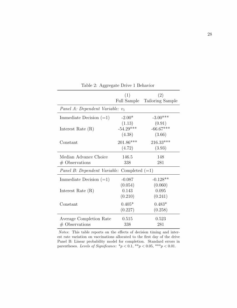
Table 2: Aggregate Drive 1 Behavior

(1) (2)Full Sample Tailoring Sample

Panel A: Dependent Variable: v1

Immediate Decision (=1) -2.00* -3.00***(1.13) (0.91)

Interest Rate (R) -54.29*** -66.67***(4.38) (3.66)

Constant 201.86*** 216.33***(4.72) (3.93)

Median Advance Choice 146.5 148# Observations 338 281

Panel B: Dependent Variable: Completed (=1)

Immediate Decision (=1) -0.087 -0.128**(0.054) (0.060)

Interest Rate (R) 0.143 0.095(0.210) (0.241)

Constant 0.405* 0.483*(0.227) (0.258)

Average Completion Rate 0.515 0.523# Observations 338 281

Notes: This table reports on the effects of decision timing and inter-est rate variation on vaccinations allocated to the first day of the drivePanel B: Linear probability model for completion. Standard errors inparentheses. Levels of Significance: *p < 0.1, **p < 0.05, ***p < 0.01.

29

3.1.2 Aggregate Preference Parameters

The raw data of Figure 3 and analysis of Table 2 indicate responsiveness of vaccinators to our

experimental parameters, R and whether allocations are Immediate or Advance. The develop-

ment of section 2 links allocation behavior and completion to these experimental parameters

via structural models of choice. In Table 3, we present parameter estimates from minimum

distance estimates from equation (1) or equations (2) and (3) when considering probabilistic

completion.

In Panel A of Table 3, we present estimates for the Full Sample under varying assumptions

for γ. In columns (1) and (2), we restrict to γ = 2, providing an aggregate benchmark for

our individual analysis which calculates individual discount factors under the assumption of

quadratic costs. Without controlling for probabilistic completion, we find β = 0.935 (s.e.

= 0.030), and reject the null hypothesis of no present bias (χ2(1) = 4.841, (p = 0.028).

Simultaneously estimating probabilistic completion increases the point estimate for both β

and δ, such that the extent of present bias falls outside of the range of standard statistical

significance (p = 0.104). The key completion parameter α is estimated precisely to be 0.003,

such that an individual assigned R = 1 who allocates 150 vaccinations to each date would be

expected to complete with probability around 0.50. A similar pattern is observed in Panel B

for the Tailoring Sample. The parameter β is estimated to be less than one, at the cusp of

statistical significance when controlling for probabilistic completion.

As the assumed degree of curvature is increased in Table 3, columns (3) through (8), both

β and δ decrease, but the general conclusions are maintained. A measure of model fit, the

criterion value, does tend to improve as γ is increased. However, increasing γ further to 3.5

generates a sharp change in the quality of fit and the completion parameter α is estimated to

be negative, inconsistent with our assumption that p(v1, v2) is declining in its arguments.39 In

principle, variation in the interest rate R, should provide an opportunity to identify γ without

restriction. Unfortunately, our minimum distance estimators did not reliably converge without

39Results available upon request.

30

restrictions. This highlights a potentially important issue with respect to the estimates of

Table 3: the estimated parameters predict more sensitivity to R than truly exists in the data.40

This mis-specification presents a clear challenge for using individual preference parameters for

tailored contracts. Having committed to a possibly mis-specified functional form ex-ante, any

success in tailoring contracts should likely be viewed as a lower bound on the potential benefits

of such initiatives.

Table 3: Aggregate Parameter Estimates, Drive 1

(1) (2) (3) (4) (5) (6) (7) (8)γ = 2 γ = 2.5 γ = 3 γ = 3.25

Panel A: Full Sample

β 0.935 0.952 0.922 0.946 0.906 0.938 0.896 0.934(0.030) (0.029) (0.040) (0.039) (0.050) (0.050) (0.055) (0.055)

δ 0.985 0.992 0.958 0.967 0.932 0.942 0.919 0.931(0.017) (0.017) (0.022) (0.022) (0.027) (0.027) (0.029) (0.030)

α 0.003 0.003 0.003 0.003(0.000) (0.000) (0.000) (0.000)

H0 : β = 1. (χ2(1)) 4.841 2.637 3.889 1.856 3.600 1.531 3.609 1.449[p-value] [0.028] [0.104] [0.049] [0.173] [0.058] [0.216] [0.057] [0.229]

Criterion Value 0.278 0.310 0.217 0.249 0.180 0.212 0.166 0.199# Vaccinators 338 338 338 338 338 338 338 338

Panel B: Tailoring Sample

β 0.969 0.970 0.962 0.963 0.954 0.955 0.949 0.951(0.018) (0.018) (0.023) (0.023) (0.028) (0.028) (0.031) (0.031)

δ 1.017 1.018 1.003 1.004 0.990 0.991 0.984 0.985(0.013) (0.013) (0.016) (0.016) (0.019) (0.019) (0.020) (0.020)

α 0.002 0.003 0.003 0.003(0.000) (0.000) (0.000) (0.000)

H0 : β = 1. (χ2(1)) 2.880 2.713 2.716 2.575 2.729 2.592 2.754 2.618[p-value] [0.090] [0.100] [0.099] [0.109] [0.099] [0.107] [0.097] [0.106]


Notes: This reports structural estimates of β, δ, and α obtained using minimum distance estimation of equations(1) in even columns or (2) and (3) in odd columns. Standard errors are reported in parentheses. Test statistic forβ = 1 with p-value in brackets. Panel A provides estimates for the Full Sample, Panel B provides estimates forthe Tailoring Sample.

40Appendix Figure A.8 reproduces Figure 3, with in-sample predictions from Table 3, column (2). Thoughthe estimates do match the responsiveness of behavior from R = 1 to R = 1.1, they do not generate the lack ofsensitivity for other changes in R.

31

3.1.3 Individual Preference Parameters

The aggregate estimates of Table 3 mask substantial heterogeneity across subjects. Following

equations (4) and (5), we calculate individual discount factors for each vaccinator assuming

quadratic costs. For those vaccinators assigned to Advance choice, this discount factor corre-

sponds to δi, while for those assigned to Immediate choice it corresponds to (βδ)i. Without

accounting for completion In Drive 1, the median [25th, 75th percentile] discount factor in

Advance choice is 1.015 [0.88, 1.18], while the median discount factor in Immediate choice is

1 [0.84, 1.21]. Accounting for completion, the median [25th,75th percentile] discount factor

in Advance choice is again 1.015 [0.88, 1.18], while the median discount factor in Immediate

choice is again 1 [0.84, 1.21]. The correlation in discount factors with and without account-

ing for completion is effectively 1, indicating probabilistic completion does not dramatically

confound any individual inferences. Indeed, the difference between the implied discount factor

with and without accounting for completion has a median [25th-75th %-ile] value of 0.00004

[-0.0002, 0.0001]. Both discount factors are used in our analysis with the relevant calculation

noted.

As noted above, an important minority of vaccinators have extreme discount factor calcu-

lations. Without accounting for completion, fifty-seven of 338 subjects in Drive 1 have implied

discount factors either above 1.5 or below 0.75.41 We term such vaccinators the ‘Boundary

Sample.’ As our tailoring exercise focuses on individuals with discount factors between 0.75

and 1.5, we restrict our individual analysis to the 281 vaccinators in the Tailoring Sample, and

discuss the Boundary Sample in robustness tests (see section 4.2). Figure 4 presents histograms

of implied discount factors for the 280 Tailoring Sample vaccinators in Advance and Immedi-

ate decisions. Two features are notable. First, in both contexts substantial heterogeneity in

discount factors is observed. The 25th to 75th percentile ranges from 0.92 to 1.15 in Advance

choice and from 0.88 to 1.15 in Immediate choice. Second, a present bias is observed in the

shape of the distributions. The one period discount factors are skewed below 1 in Immediate

41Such extreme behavior is slightly more pronounced in Immediate choice (34 vaccinators) relative to Advancechoice (23 vaccinators), (t = 1.84, p = 0.07).

320

510

1520

.75 .85 .95 1.05 1.15 1.25 1.35 1.45 .75 .85 .95 1.05 1.15 1.25 1.35 1.45

Advance Choice Immediate Choice

Perc

ent

Drive 1 Discount Factors

Figure 4: Individual Discount Factors in the Tailoring Sample

Notes: This figure provides histograms of one period discount factors calculated from equation (4) separately for subjects in theAdvance Choice condition (left panel) and the Immediate Choice condition (right panel). The sample is restricted to vaccinatorsin the Tailoring Sample (vaccinators with R∗i ≥ 0.75 or R∗i ≤ 1.5). Calculating discount factors from equation (5) accounting forprobabilistic completion yields an identical figure.

relative to Advance choice. A Kolmogorov-Smirnov test for equality of distributions sits at the

cusp of statistical significance (DKS = 0.15, p = 0.10).

The observed heterogeneity in discount factors across vaccinators resonates with prior ex-

ercises demonstrating heterogeneity of preferences even with relatively homogeneous samples

(see e.g., Harrison et al., 2002; Ashraf et al., 2006; Meier and Sprenger, 2015). Further, this

heterogeneity is precisely the reason there is promise in tailoring contracts individually.

33

5010

015

020

025

0

50 70 90 110 130 150 170 190 210 50 70 90 110 130 150 170 190 210

Untailored Tailored

Allocation Target Target (Completion Adjusted)

Day

2 V

acci

natio

ns

Day 1 Vaccinations

Panel A: Allocation Behavior.4

5.5

.55

.6

.8 1 1.2 1.4 .8 1 1.2 1.4

Untailored Tailored

Linear Fit of Actual Completion Predicted Completion Rate

Com

plet

ion

Rat

e

Discount Factor

Panel B: Completion Rate

Figure 5: Discounting and Tailoring

34

3.2 Tailored Contracts

Individual discount factors from Drive 1 in hand, we turn to the possibility of tailoring intertem-

poral contracts to individual preferences. Of the 281 vaccinators in the Tailoring Sample, 280

participated in Drive 2.42 Of these, 142 vaccinators were assigned a value of R equal to their

discount factor. That is, tailored vaccinators were assigned R∗i = (β1d=1,iδ)i, from equation

(4), which should induce equal provision of effort through time, v1,i = v2,i. Given the minute

differences between implied discount factors with and without controlling for completion, this

policy target is effectively identical regardless of whether the discount factor from equation (4)

or equation (5) is used. The remaining 138 vaccinators serve as control and were assigned a

uniform random interest rate Ri ∈ U [0.75, 1.5].43

Figure 5, Panel A plots vaccinations allocated to the first day of the drive against vaccina-

tions allocated to the second day of Drive 2 separately for the tailored and the untailored group.

Notable from Figure 5 is the relative dispersion of the untailored controls around the 45-degree

line of equal provision relative to the tailored treatments. Also graphed in Panel A for the tai-

lored group is the policy target accounting for probabilistic completion. This line is effectively

indistinguishable from the 45 degree line such that whether one accounts for completion or not,

the policy should induce smooth allocations.

We examine differences in the distance from the 45-degree line using the metric |v1,iv2,i− 1|,

the absolute percentage difference between v1 and v2. The mean distance for the untailored

group is 0.61 (s.d. = 3.64) while the mean distance for the tailored group is 0.14 (s.d. = 0.23),

t278 = 1.54, (p = 0.13). The lack of statistical significance is due primarily to several substantial

distance outliers. Trimming the top and bottom 1% of the sample of Drive 2 allocations, the

mean distance for the untailored group is 0.15 (s.d. = 0.19), while the mean distance for the

tailored group is 0.10 (s.d. = 0.11), t265 = 3.07, (p < 0.01).

42Vaccinators from the boundary sample were allowed to participate in Drive 2 and were either assignedRi ∈ U [0.75, 1.5] if they were in the untailored control group (31 subjects) or assigned Ri = 0.75 or Ri = 1.5 ifthey were in the tailored group and had R∗

i < 0.75 (15 subjects) or R∗i > 1.5 (11 subjects). See section 4.2 for

analysis of the boundary sample.43As noted in section 2.3, assignment to the tailored or the untailored group was conducted via stratified

randomization with strata based upon the tercile of differences from equal provision of effort in Drive 1.

35

In Table 4, we provide corresponding least squares regression analysis. Following best

practice for such analysis (Bruhn and McKenzie, 2009), we control for fixed effects for each

stratum in the stratified randomization. In column (1), we analyze all 280 subjects and note

a sizable reduction in distance under tailoring that falls just outside the range of significance.

Echoing our raw results, when excluding outliers in column (2), we find that tailoring serves

to reduce distance from equal provision significantly by around six percentage points. Relative

to the untailored controls, tailoring reduces distance from equal provision by around one-third,

indicating substantial benefits to our tailored policy initiative. In column (3), we additionally

control for the value of R∗i or Ri assigned in Drive 2. This regression identifies whether tailoring

generates more equal provision for a given value of R, and hence controls for any differences in

interest rates across tailored and untailored groups. Again, tailoring serves to reduce distance

significantly.

Vaccinators assigned to Advance choice in Drive 1 remain in Advance choice in Drive 2,

while those assigned to Immediate choice remain in Immediate choice. In columns (3)-(6) of

Table 4, we examine differential effects of tailoring across these two groups. Given that the

individual discount factors skew lower in Immediate choice, one might expect larger distance

measures in Immediate controls (and hence greater benefits to tailoring). This is precisely

what is observed. Untailored Immediate choice is associated with significantly larger distance

measures and tailoring for Immediate choice significantly reduces these distances. In columns

(5) and (6), excluding outliers, we find that tailoring in Immediate choice reduces distance from

equal provision by around one-half. Note that this effect size (8.4 percentage points) is similar

to the effect of moving a vaccinator from advance to immediate choice in the untailored group

(8 percentage points). Tailoring in Advance choice appears to directionally reduce distance as

well, but the effect is not significant, potentially due to the relatively small average distance

measure identified in untailored Advance choice.

In addition to allocation behavior, we can use individual discount factor measures from

equation (5) in Drive 1 to predict completion probabilities out-of-sample for Drive 2. Our

36

Table 4: The Effect of Tailoring Intertemporal Incentives

Dependent variable: |v1,i

v2,i− 1|

(1) (2) (3) (4) (5) (6)

Tailored (=1) -0.489 -0.059*** -0.049*** -0.070 -0.019 -0.014(0.321) (0.019) (0.018) (0.069) (0.019) (0.019)

Immediate Choice (=1) 0.982* 0.125*** 0.117***(0.573) (0.035) (0.035)

Tailored x Immediate -0.888 -0.090** -0.084**(0.604) (0.040) (0.040)

Constant 1.407 0.159*** 0.022 0.873 0.094*** -0.004(0.860) (0.023) (0.058) (0.552) (0.026) (0.057)

Stratum FEs Yes Yes Yes Yes Yes YesExclude 99th and 1st Percentiles No Yes Yes No Yes Yes

Drive 2 R∗i or Ri No No Yes No No Yes

R-Squared 0.035 0.060 0.082 0.053 0.142 0.154Mean in Untailored Contract 0.612 0.153 0.153 0.612 0.153 0.153Mean in Untailored Advance 0.089 0.089 0.089Mean in Untailored Immediate 0.701 0.169 0.169# Vaccinators 280 267 267 280 267 267

Notes: This table reports the effects of tailoring on the equality of effort provision over time. The measure | vtvt+1− 1|

(the percentage difference between tasks allocated to day 1 and day 2 of the drive) reflects the distance of the taskallocation (v1,v2) from equality (v1 = v2). Column (1) reports a regression of this measure on an indicator equal toone for subjects in the tailored group. Column (2) reports estimates from the same specification excluding outliers.Column (3) controls for the interest rate assignment in round 2. Column (4) provides estimates on the same sample ascolumn (1) interacting treatment with being in the immediate choice condition. Columns (5) and (6) apply the samerestrictions to the sample as columns (2) and (3) respectively. Ordinary least squares regressions. Heteroskedasticityrobust White standard errors reported in parentheses. *p < 0.1, **p < 0.05, ***p < 0.01.

37

tailored policy links individual discount factors to assigned interest rates. Impatient subjects

‘pay’ for their impatience with lower values of R∗i . Given the intertemporal constraint v1 +

R∗i · v2 = 300, this means less patient individuals will ultimately have to do weakly more

work. Under our assumed functional form for p(v1, v2) this implies a relationship between

completion probabilities and patience. In the tailored group, less patient individuals should

be substantially less likely to successfully complete their Drive 2 targets. In Figure 5, Panel

B, we plot the predicted completion rate in Drive 2 against the individual discount factor.

A tight relationship between patience and predicted completion exists in the tailored group,

and no discernible relationship exists for the untailored group. In Panel B, we also plot the

linear fit from the regression of realized Drive 2 completion against discount factors.44 Closely

matching the prediction, true completion probabilities are positively correlated with discount

factors under the tailored contract terms, but are effectively unrelated to discount factors for

the untailored group.

Table 5 provides corresponding logit regressions showing a significant positive relationship

between discounting and completion only for the tailored group of subjects. Table 2 also

provides actual and predicted completion rates separately for tailored and untailored subjects.

The two groups are predicted to differ in their completion rates due to different contract terms45,

and they indeed do differ in the predicted direction. Overall, predicted and actual completion

rates are significantly correlated, as those individuals who actually do fail were predicted to do

so with higher probability, 0.521 (s.e. = 0.002) vs 0.509 (0.002), t335 = 3.80, (p < 0.01).46

4 Robustness Tests and Additional Exercises

The analysis to this point indicates three key findings. First, there appears to be a present bias

in vaccinator allocation behavior. Those individuals making Immediate choice allocate fewer

44Though based on a linear probability model, this fitted value is restricted to be the expectation conditionalon being in the interval (0,1).

45Due to the random uniform assignment the untailored group has relatively more interest rates above 1.46For the Tailoring sample alone, these values are 0.520 (s.e. = 0.003) vs 0.512 (0.002), t278 = 2.30, (p < 0.05)

38

Table 5: Tailoring, Discount Factors, and Completion

Dependent variable: Drive 2 Completed (=1)

Untailored Tailored(1) (2) (3) (4)

Drive 1 Discount Factor 0.693 0.152 2.506** 2.312**(1.049) (1.086) (1.043) (1.069)

Constant -0.533 0.118 -2.780** -2.516**(1.082) (1.131) (1.120) (1.150)

# Vaccinators 138 132 142 135Log-Likeliihood -94.908 -90.254 -95.022 -91.078Exclude 99th and 1st Percentiles No Yes No YesActual Completion Rate 0.543 0.568 0.458 0.474Predicted Completion Rate 0.524 0.523 0.508 0.508

Notes: This table reports logit regressions for successful completion in Drive 2 on Drive 1discount factor for tailored and untailored subjects. Individual discount factor calculatedfrom equation (5) based on Drive 1 allocation. Predicted completion rate calculated asp(v1,i, v2,i) at predicted Drive 2 allocation (v1,i, v2,i). Heteroskedasticity robust Whitestandard errors reported in parentheses. *p < 0.1, **p < 0.05, ***p < 0.01.

vaccinations to v1 than those making Advance choice. Second, despite the general tendency

towards less patience in Immediate choice, substantial heterogeneity in discounting is observed.

Both of these effects resonate with prior experimental findings and highlight the potential for

policy interventions tailored to individual preferences. Third, tailored contracts work. Those

individuals given a tailored interest rate equal to their previously measured discount factor

provide smoother service than untailored controls. Furthermore, our tailored contracts generate

additional predictions with regards to completion probabilities which are also borne out in the

data. In the following sub-sections, we explore robustness to a set of plausible alternative

interpretations and provide a set of natural additional examinations.

4.1 Repeated Measurement and Within-Subject Variation

In Drive 1, when relying on between subjects tests, statistical tests of present bias fall at the cusp

of significance. Given the wide heterogeneity in observed patience regardless of decision timing,

39

one may fail to statistically identify present bias even if it exists on average. Indeed, most studies

of present bias and dynamic inconsistency are conducted as within-subject exercises with more

choices, potentially because of such wide heterogeneity.

Fortunately, our failed Drive 0 and the corresponding re-randomization in Drive 1 allows

us to identify present bias using both more data and within-subject variation for vaccinators

who changed from Advance to Immediate choice (or vice versa) across drives. Appendix Table

A.3, reconducts the analysis of Table 3, columns (1) and (2) using this augmented data set.

First, we analyze all potential observations, drawing from 622 choices made by 390 vaccinators

in either Drive 0 or Drive 1.47 There, we estimate β = 0.903 (clustered s.e. = 0.030) and reject

the null hypothesis of no present bias at all conventional levels, χ2(1) = 10.571, (p = 0.001)

when controlling for probabilistic completion. The estimated degree of present bias corresponds

closely with other recent estimates of working over time from laboratory studies Augenblick et

al. (2015); Augenblick and Rabin (2015). Examining, only our panel of 232 individuals who

participated in both Drive 0 and Drive 1, a similar estimate is obtained β = 0.931 (0.032),

χ2(1) = 4.497, (p = 0.034). This significant degree of present bias is driven by within-subject

variation. For those individuals who transition from Advance to Immediate Choice or vice-

versa across drives we find β = 0.912 (0.042), and reject the null hypothesis of no present

bias χ2(1) = 4.344, (p = 0.037). As with our aggregate estimates, when identifying only from

between-subject variation, though present bias is of similar magnitude, precision remains an

issue.

Repeated measurement from our panel of subjects provide for two additional analyses. First,

the 126 subjects who change from Advance to Immediate choice provide an opportunity to

investigate present bias at the individual level. Following equation (4), we calculate a discount

factor for each condition the vaccinator faces. The parameter δ is identified as the discount

factor from Advance choice while β is identified as the discount factor from Immediate choice

divided by that of Advance choice. Interestingly, as in our analysis of discount factors, we find

47Only Drive 1 completion data is used to estimate the completion function given the noted cell networkissues that generated the challenges for Drive 1.

40

δ is centered around 1 with a median value of 1.04, and that β is skewed below 1 with a median

value of 0.95. Sixty-nine (54.8%) of 126 vaccinators have β < 1, 6 (4.8%) have β = 1, and 51

(40.5%) have β > 1. A sign test for the null hypothesis that the median β is equal to 1 yields a

p-value of 0.12 (two-sided test).48 Together, these results show that general patterns of present

bias are observed at the aggregate and individual level when investigating only within-subject

variation in a sub-sample of 126 vaccinators who change between Advance to Immediate choice

across conditions. See Figure A.9 for graphical detail.

Second, for the 106 vaccinators who maintain their Advance or Immediate choice assignment,

we have two discount factor measures from Drive 0 and Drive 1. One-hundred five of these

subjects also participated in Drive 2. An important question for such subjects is what is

the additional value of having a second measure of preferences. Are improved predictions of

behavior made? To answer this question, we derive the predicted value of v1,i for the preferences

identified in Drive 0 and Drive 1.49 In Appendix Table A.4, we regress the actual allocation

on predicted allocations separately for tailored and untailored subjects. For tailored subjects,

there appears to be little additional value of incorporating the Drive 0 measures, while for

untailored subjects the Drive 0 measures are even more predictive than those in Drive 1. In

either case, the value added of additional measures is limited as the R-squared obtained with

the single more predictive measure is over 95% of that obtained with both. This suggests

that the marginal value of additional observations (particularly for those we attempt to tailor)

declines rather sharply in this context.

48For the one-sided test with an alternative of β < 1, the p-value is 0.06. Excluding a single subject with βin excess of 19 reduces the two-sided (one-sided) p-value to 0.10 (0.05).

49Following equation (4), the predicted allocation to v1 is calculated as

v1,i =(β1d=1,iδ)i

R2

1 + (β1d=1,iδ)iR2

.

41

4.2 Structural Assumptions

As in any structural exercise, a set of assumptions are required to infer discounting parameters

from vaccinator allocation behavior. Six assumptions are relevant for the present discussion,

which we discuss below.

Assumption 1: Stationarity of the Cost Function: We assume the cost function is the same for

day 1 and day 2. If sooner costs are forecasted to be more severe than later costs, vaccinators

may appear disproportionately impatient, while if later costs are forecasted to be more severe,

they may appear disproportionately patient. Further, if perceived costliness of vaccinations

changes from Advance to Immediate choice, present bias measured by β is conflated with non-

stationarity.

Importantly, our monitoring technology provides time-stamps and geo-stamps for vacci-

nation activity. Time stamps are recorded every vaccination attempt, while geo-stamps are

collected approximately every 10 vaccination attempts. This may provide independent means

for assessing the costliness of tasks from time use. For each vaccinator, we identify the median

time lapse between vaccination attempts and the median distance covered per 30 minute win-

dow each day.50 Of our 338 vaccinators, measures for median time lapse between vaccination

attempts are available for 277 on either Day 1 or Day 2 and for 228 vaccinators on both days

of Drive 1.51 Of our 338 vaccinators, measures for median distance traveled every 15 minutes

50We focus only on the distance traveled and time taken for vaccinations between 8 am and 6pm each day.The distribution of time taken and distance traveled carried some extreme outliers for some subjects. As such,we felt the median was an appropriate summary statistic. Though we had expected to receive geo-stamp dataapproximately every 10 vaccination attempts, when the monitoring data arrived we noted substantial variancein the number of vaccinations with common geo-stamps and sequences of geo-stamps which ‘bounced’ back andforth between geographic coordinates. In order to not overstate subject movements, we opted to take averagecoordinates within a 15 minute window and calculate direct-line distance between window-average coordinatesas our measures of distance.

51265 vaccinators have Day 1 lapse data while 240 have Day 2 lapse data. Of the 73 vaccinators with missingDay 1 data, 68 completed either zero or one vaccination on Day 1 such that time lapse between vaccinationattempts is not calculable. The remaining 5 conducted vaccinations but did not have phones that interactedwith the server to report time use. Of the 98 vaccinators with missing Day 2 data, 92 of them completed eitherzero or one vaccination on Day 2 and the remaining 6 did not have phones that interacted with the server toreport time use. Those vaccinators who completed vaccinations but did not have interaction with the serverhad their vaccination records pulled manually from their phones after the drive.

42

are available for 274 on either Day 1 or Day 2 and for 226 vaccinators on both days of Drive

1.52

Vaccinators take around 3.4 minutes between vaccination attempts and walk around 0.06

miles per 15 minutes on Day 1. Focusing on individuals with measures on both days of the

drive, we find that time taken and distance traveled are uncorrelated both with Advance

choice and with discount factors within condition. Time and distance are also uncorrelated

with Advance choice and discount factors on Day 2 of the drive. Further, differences in

time taken or distance walked are statistically indistinguishable from zero, uncorrelated

with allocation timing, and uncorrelated with discount factors within condition. These data

indicate stability in required average effort per vaccination which is unrelated to assignment

to Advance or Immediate choice, and that changes in efficacy are unrelated to measured

preferences. This suggests that perceived changes in costs likely do not drive our measures of

patience or our finding of present bias.53 These results are all presented in Appendix Table A.5.

Assumption 2: Unobserved Idiosyncratic Costs: We assume that vaccinations are the only

argument of costs when identifying time preferences. However, there may be idiosyncratic costs

across time or individuals that could influence measured patience. For example, a vaccinator

with an appointment lasting 2 hours on Day 1 and no appointments on Day 2 may find it

extremely costly to allocate vaccinations to Day 1. This may appear to the researcher as

impatience, but only reflects the vaccinator’s idiosyncratic costs across days. Further, if such

idiosyncratic events are easier to re-organize when making Advance choice, present bias may

be conflated with ease of scheduling.

52257 vaccinators have Day 1 distance data while 240 have Day 2 distance data. Of the 81 vaccinators withmissing Day 1 data, 75 completed four or fewer vaccination attempts on Day 1 such that distance traveledbetween 15 minute windows is not calculable. The remaining 6 conducted vaccinations but either did not havephones that interacted with the server to report location or had faulty Global Position Systems (GPS) in theirphones. Of the 98 vaccinators with missing Day 2 data, 96 of them completed four or fewer vaccination attemptson Day 2 and the remaining 2 did not have phones that interacted with the server to report location or hadfaulty GPS.

53Ultimately, such stationarity is likely to be expected given that vaccinators are already well-versed invaccination procedures, have an average of 10.5 years of experience as vaccinators, and received a half day’straining on the vaccination monitoring application.

43

Here, again, the additional data on vaccinator time use available from the monitoring

application is potentially valuable. We can investigate whether extended periods of non-

vaccination exist and if they are correlated with measured preferences and allocation timing.

As in the example above, a vaccinator with an extended period of non-vaccination may well

be experiencing forecasted idiosyncratic costs unrelated to vaccinations. Appendix Table A.6

repeats the analysis from Appendix Table A.5, with dependent variables of the maximum

daily time lapse between vaccination attempts and whether the longest daily break is in

excess of two hours. Longest daily breaks are, on average, around 59 minutes on Day 1 with

around 13% of vaccinators taking longest breaks in excess of 2 hours. Focusing on individuals

with measures on both days of the drive, we find that the length of longest breaks and the

probability of 2 hour breaks are uncorrelated with Advance choice and uncorrelated with

discount factors within condition. Almost identical patterns are observed on Day 2 of the

drive. Differences in break behavior across days are statistically indistinguishable from zero,

uncorrelated with allocation timing, and uncorrelated with discount factors within condition.

These data suggest that idiosyncratic costs identified from taking extended breaks do not

explain the extent of impatience in the sample, and that potential difficulties in rescheduling

do not explain observed present bias.

Assumption 3: Probabilistic Completion: Our exercise assumes that indivduals know the map-

ping from vaccinations to completion probabilities and trade off discounted marginal costs

and marginal failure probabilities. Two important functional form assumptions inform our

development. First, we assume the failure probability (known to the vaccinator) is given by

p(v1, v2) = 1αv1

1αv2

. In Appendix Table A.7, we reconduct the analysis of Table 3, Panel A with

two alternate functional forms for p(v1, v2). First, we assume p(v1, v2) = 11+α′(v21+v22)

. Second,

we assume p(v1, v2) = 11+α′′(v31+v32)

. Both functional forms carry the property that failure prob-

abilities are declining with the volume of work as long as α′, α′′ > 0. They differ only in the

marginal tradeoffs they entail. Very limited differences are observed in aggregate estimates

44

across these functional forms and the one used in the main text. Additionally, when assuming

γ = 2, the pairwise correlations between individual discount factor measures using these three

functional forms all exceed 0.99.

Our exercise additionally restricts the net utility of completion, [δ2u(1000)−vγ1−β1d=1δ ·vγ2 ],

to be equal to 100. In Appendix Table A.8, we reconduct the analysis of Table 3, Panel

A assuming this net utility equal to 1000 or to 10000. Only small changes in the aggregate

estimates are observed. Furthermore, at the individual level when assuming γ = 2, the pairwise

correlations between individual discount factor measures using these three net completion utility

values all exceed 0.99.

Though our exercise assumes individuals know the relationship between allocations

and failure probabilities under a given cost function, a plausible alternative is that costs

are uncertain. The natural evolution of uncertainty through time may lead to differences

in measured preference parameters across groups. Though the resolution of uncertainty

may lead to apparent dynamic inconsistency, the direction is not clear. Some vaccinators

may grow more patient as uncertainty is resolved, some less so. Naturally, if shocks to

costs do underly our observed differences in patience across individuals, one might not ex-

pect to be able to tailor contracts at the individual level over time with the success that we have.

Assumption 4: Identical Cost Functions: Our aggregate exercise assumes identical costs

across subjects, and our individual elicitation assumes identical quadratic costs. Though

these assumptions allow for straightforward estimation and calculation of time preferences,

any violation would lead us to confound differences in patience across individuals or across

allocation timing with differences in costs. One natural view would be to assume that

individuals do not discount at all, δ = 1 and β = 1, such that allocations identify only the

shape of the cost function. In this case, when R = 1, all vaccinators, regardless of allocation

timing, should exhibit v1 = v2 = 150 for all values of γ.54 Examining the Drive 0 and Drive

54This is because the Euler equation reduces to (v1v2 )γ = R = 1, which implies v1v2

= 1.

45

1 data, we find that for 163 vaccinators who were assigned R = 1, the mean allocation is

v1 = 140.84 (s.d. = 24.76).55 Though the median allocation is indeed 150, responses range

widely with 5th-95th percentiles of response being 103 to 160. If heterogeneity in costs were

driving response and discounting was not a key feature of the data, one would not expect to

see this extent of variation in response when R = 1. Further, given random assignment to

allocation timing, heterogeneity in costs does not easily rationalize the observed present bias

in the data.

Assumption 5: Only Failure, No Shirking: Our structural exercise assumes individuals know

their likelihood to succeed and work only some minimal amount (e.g., that associated with

the outside option) in the case where their target is not attainable. Appendix Figure A.6

demonstrates the plausibility of this assumption with a bimodal pattern of almost complete

success and almost complete failure. Another possibility is that subjects find an alternate way

to renege on their contracts by shirking and still receiving pay. Not all vaccination attempts

are equally challenging. In Appendix Figure A.7 we plot for each half-hour of Drive 1 the

total number of attempted vaccinations along with the probability of successful vaccination

and the probability that no child was reported as present. Reporting that no child was present

is likely to be less time consuming than a successful vaccination and easier to falsify. The

vast majority of vaccination activity occurs before 3:00pm, there exists no sharp uptick in

activity as days end, and we find evidence that vaccinators’ proportion of successful or failed

vaccination attempts remains largely steady throughout the workday. This suggests that

allocated vaccination attempts are conducted with due diligence.

Assumption 6: No Biases in Choice: Our study assumes that the allocation environment

itself induces no biases in choice such that vaccinator allocations are directly informative of

preferences. A substantial literature in experimental economics suggests that aspects of the

5542 of 163 vaccinators allocated exactly v1 = v2 = 150.

46

decision environment may deeply influence measures of preferences (for recent examples, see

Harrison, Lau, Rutstrom and Sullivan, 2005; Beauchamp, Benjamin, Chabris and Laibson,

2015). One common view is that subjects are biased towards the middle of a choice set. In

our environment, this could involve subjects opting for either equal allocations of v1 = v2,

or choosing an allocation in the middle of their budget constraint, v1 = Rv2. Only 31 of 338

vaccinators (9%) exhibit v1 = v2. Taking a less conservative measure of v2−2.5 ≤ v1 ≤ v2 +2.5,

we find that still only 58 of 338 vaccinators (17%) are within 5 vaccinations of v1 = v2.56 Only 35

of 338 vaccinators (10.3%) exhibit v1 = Rv2. Taking a less conservative measure of Rv2−2.5 ≤

v1 ≤ Rv2 +2.5, we find that 83 of 338 vaccinators (25%) are within 5 vaccinations of v1 = Rv2.57

Taken together, this suggests that biases towards the middle of the budget constraint or towards

equal allocation are unlikely to be driving substantial portions of allocation behavior.

4.3 Tailoring Robustness Tests

Our Drive 2 data show that vaccinators who are given bonus contracts with a value of R equal

to their estimated discount factors provide significantly smoother service. Here we examine

robustness of this result to alternative comparison groups, alternative measures for smoothness

in service provision, and alternative measures for treatment. We conclude the section by pro-

viding results from a set of additional exercises assessing the value of atheoretic approaches to

tailoring, and the possibility for alternative interventions based on different policy preferences.

4.3.1 Alternative Comparison Groups

Our results demonstrate that, relative to a comparison group with uniform random values of R,

tailoring serves to reduce distance to the policy target by around one-third. A natural question

is whether these tailoring benefits are observed relative to alternative controls. In Appendix

Table A.9, we present three additional analyses. A first natural control is the use of a single

value of R applied to all individuals. Unfortunately, it is not possible to compare only a single

56As an even less conservative measure, 145 of 338 (43%) satisfy v2 − 10 ≤ v1 ≤ v2 + 10.57As an even less conservative measure, 137 of 338 (40.5%) satsify Rv2 − 10 ≤ v1 ≤ Rv2 + 10.

47

value of R given our uniform random assignment protocol. However, we can examine a section

of the untailored group around a given value. In column (1) of Table A.9, we repeat the analysis

of Table 4, column (3), but use as the comparison group only those untailored vaccinators who

received a value of R within one standard deviation of their group’s mean R∗i of 1.036. Tailoring

continues to decrease the distance from smooth provision relative to this more limited control

group. In column (2), we repeat this analysis excluding those individuals from the untailored

group who randomly received a value of Ri within 0.10 of their true value of R∗i . The benefits

of tailoring are observed with increased precision.58 A second potential control group would be

a subset of the untailored group who receive the same distribution of R as those in the tailored

group. Matching on the 1st, 5th, 10th, 25th, 50th, 75th, 95th and 99th percentiles, column (3)

demonstrates that relative to a control group receiving a matched distribution of R, tailoring

continues to significantly reduce the distance from smooth provision.

4.3.2 Tailoring and Completion

Our analysis to here treats probabilistic completion through the lens of a structural model

and attempts to assess the trade-off between marginal completion probabilities and discounted

marginal costs. Though this analysis seems both tractable and yields valuable predictive in-

sights, an alternative interpretation for failure exists. If the outcome of failure is perfectly

forecasted by the vaccinator, there is no incentive to respond truthfully. As such, the targets

set in Drive 1 and our corresponding inference on time preferences would be systematically inac-

curate for individuals expecting to fail. In effect, successful vaccinators are allocating according

to equation (1), while unsuccessful vaccinators are providing only noisy response. Under this

assumption, we should be dramatically less able to predict allocation behavior for vaccinators

who fail in Drive 1.

Table A.10 repeats the analysis of Table 4, columns (1) through (3) separately for subject

58Comparing tailored individuals to those who received close to the untailored group’s mean value of R∗i is

important because, in principle, the mean value of R∗i should yield smooth provision for the average subject.Not only is the average distance for these comparison groups substantial, 0.132 to 0.150, but the tailoring yieldsadditional benefits at the individual level by leveraging the heterogeneity in discount factors across vaccinators.

48

who completed and failed to complete their Drive 1 targets. Similar magnitude effects are

observed for both sets of subjects, with tailoring serving to reduce distance from the equal

provision by around one third. Focusing only on the completing subjects, we would reach

effectively the same conclusion as our initial analysis. Furthermore, the fact that predictive

accuracy remains for subjects who fail to complete demonstrates that there is content to the

allocations subjects make regardless of ex-post completion.

4.3.3 Alternative Measures for Smooth Provision

Our analysis measures the distance to equal provision using the metric |v1,iv2,i− 1|. In Table

A.11, we reconduct the analysis of Table 4, using five alternate measures for smoothness.

Panel A presents the Euclidean distance to the 45 degree line,|v1,i−v2,i|√

2. Panel B presents

the Euclidean distance normalized by the total number of vaccinations allocated,|v1,i−v2,i|√2(v1,i+v2,i)

.

Panel C presents the number of sooner vaccinations that would need to be reallocated to reach

the 45 degree line, |v1,i − 3001+R|. Panel D presents probit regressions for needing to reallocate

more than 25 vaccinations, |v1,i − 3001+R| > 25. And finally, Panel E presents the value of the

policymaker’s objective function, min[v1,i, v2,i]. Across all specifications, the main conclusions

are reproduced. However, the results with respect to additional tailoring benefits in Immediate

choice fall, at times, outside the range of statistical significance. These alternative measures

of smooth provision indicate that our results on the potential benefits of tailoring are not an

artifact of how one measures the outcome of interest.

4.3.4 Alternative Sample Restrictions and Treatment Measures

Our tailoring exercise focused on vaccinators with discount factors between 0.75 and 1.5. Of

337 vaccinators in Drive 2, 280 satisfied this requirement. Those vaccinators whose discount

factors fell outside of this range were given either R = 0.75 or 1.5 depending on which bound

they were closest to. For such individuals, tailoring is not a binary treatment, but rather a

continuous difference between their discount factor and the exogenously given one. Indeed,

49

for all vaccinators in the untailored group, treatment is also a continuous measure. In Table

A.12, Panel A, we reconduct the analysis of Table 4 using as the measure of treatment the

absolute difference between each vaccinator’s discount factor and their assigned interest rate,

which we label Tailor Intensity. The main results are reproduced; the closer discount factors

are to interest rates, the smoother is provision.59 In Panel B, we include those individuals

in the Boundary Sample with discount factors that lie outside of the bounds of interest rate

assignment. Including these observations does not alter the conclusions; however, it should be

noted that treatment is no longer orthogonal to individual preferences as extremely patient and

impatient vaccinators will receive larger treatment intensity on average.60

4.3.5 Atheoretic Approaches

Our exercise demonstrates that structural estimates of time preferences can be useful in pre-

dicting subsequent behavior. An alternative to developing a structural model of choice would

rely on the researcher recovering the relationship between key parameters of interest, R and

1d=1, and behavior, and developing a subsequent prediction without filtering the relationship

through the structural model.

We examine one example of such an exercise. For Drive 1 behavior, we recover the rela-

tionship between v1 and R and 1d=1 by conducting a Least Absoluate Shrinkage and Selection

Operator (LASSO) regression with penalty parameter chosen via 10-fold cross validation (Tib-

shirani, 1996) of v1 on a cubic polynomial in R interacted with 1d=1.61 The corresponding

selected lasso coefficients deliver an atheoretic representation of the most predictive (in terms

of cross-validated mean squared error) relationship between v1 and key parameters of interest in

Drive 1. Given the values of R and 1d=1 provided in Drive 2 and the Drive 1 lasso coefficients,

59Restricting attention only to the untailored group reveals directionally similar, though insignificant, resultsacross all specifications.

60Using the indicator for tailoring would not be an appropriate solution to this problem as tailored vaccinatorswith extreme patience or impatience may actually receive interest rates that are further from their policy-optimalinterest rates than those in the untailored condition.

61The provided regressors are a constant and normalized values of R,R2, R3,1d=1, R× 1d=1, R2 × 1d=1, and

R3×1d=1. The lasso regression and cross-fold validation procedure were implemented using the glmnet packagein R.

50

we predict the Drive 2 value of v1 for each individual.62 Similarly, we predict Drive 2 value

of v1 from the assigned values of R and 1d=1 and the individual discount factor identified in

Drive 1 from equation (4). In Appendix Figure A.10 we examine the predictive validity of the

structural versus the non-structural approaches by plotting predicted and actual values of v1 in

Drive 2 for the 337 subjects who participated in both Drive 1 and Drive 2. We also provide non-

parametric lowess curves for the relationship between predicted and actual values.63 Notable

from Appendix Figure A.10 is the generally close adherence between structurally predicted and

actual values. The lowess line follows the 45 degree line of perfect prediction through the ma-

jority of the space. Less adherence is observed between non-structural predictions and actual

behavior. The structural predictions deliver higher correlations with real behavior (ρ = 0.18)

than do the non-structural predictions (ρ = 0.16) and lower bias in prediction (27.9 vs. 32).

However, the root mean squared error is lower for the non-structural predictions (32.8 vs 39.1).

Hence, on the basis of bias and correlation, our structural exercise outperforms the machine

learning lasso algorithm trained on Drive 1.

There is an additional important difference between the LASSO and structural predictions

presented here. The structural prediction for a given vaccinator’s behavior in Drive 2 derives

from their allocation in Drive 1 and the interest rate assigned in Drive 2. It therefore relies on

a single data point. By contrast, the LASSO prediction for a given vaccinator is derived by

training a model on the entire cross-section of data from Drive 1, and then obtaining a fitted

value based on the interest rate assigned in Drive 2. This means the LASSO prediction will

be identical for all subjects assigned the same interest rate while the structural prediction may

vary depending on individually measured preferences. Hence, the two methods are not only

different in the sense of being structural or atheoretic, they also differ both in the amount of

data informing the prediction and in the extent of heterogeneity they can predict.

62Note that this prediction will be identical for all vaccinators given the same value of R and 1d=1, and hencewill mispredict any heterogeneity across vaccinators.

63The lasso procedure on Drive 1 selects an intercept and R as delivering coefficients of sufficient size giventhe cross-validated constraint choice.

51

4.3.6 Alternative Policy Preferences

While our results suggest that tailored contracts can improve success in achieving a Leontief

policy objective, a natural question is whether this approach could be put to use to achieve

other policy objectives. Ultimately, any attempt to tailor contracts will rely on whether ini-

tially elicited preferences are stable. If vaccinator time preferences are stable, then changes in

incentives will have predictable effects on behavior.

To provide a general assessment of the promise of alternative policy objectives, we examine

the stability of identified discount factors across Drives 1 and 2 by calculating the corresponding

discount factor from equation (4) for each vaccinator in each Drive. Figure A.11 presents the

calculated discount factors for Drive 1 and Drive 2 along with the 45 degree line for 317 of

337 vaccinators.64 The correlation in discount factors across rounds is ρ = 0.41, (p < 0.01),

indicating stability in preferences.65 Our findings correspond with those of Meier and Sprenger

(2015), who investigate subjects participating in an identical monetary discounting experiment

approximately one year apart and identify a one-year correlation of around 0.5 for monetary

choices. The level of correlation in discount factors across drives indicates stability in preferences

such that alternative policy objectives may also be achievable with tailored contracts.66

5 Conclusion

Structural parameters for intertemporal preferences have been at the center of theoretical and

empirical research modeling intertemporal choice for much of the last century. This paper

64Eliminated from the figure and from our calculations of stability are 20 vaccinators with discount factorsin excess of two in one or both drives.

65Including the remaining 20 extreme vaccinators, the correlation changes substantially to ρ = 0.01, (p =0.87). It should be noted that the correlation in identified discount factors is substantially higher in the tailoredcondition, ρ = 0.67, (p < 0.01), relative to the untailored condition, ρ = 0.17, (p < 0.05). We believe this is dueto some sensitivity of behavior to extreme values of R in Drive 2. For untailored subjects who coincidentallyreceive a value of Ri within 0.25 of their value of R∗

i , the correlation in discount factors is ρ = 0.53, (p < 0.01).66One natural alternative is to maximize performance, regardless of timing. In such a case, we consider a

policymaker with linear preferences, P (v1, v2) = v1 +v2, who wishes to maximize the total number of completedvaccinations regardless of timing. Maximizing this objective function subject to the vaccinator’s offer curve,yields an optimal R∗

max =√β1t=1δ(1 + β1t=1δ)− β1t=1δ. Unfortunately, our assigned values of R are generally

quite far from R∗max making it difficult to test for the possibility of a maximizing contract.

52

seeks to understand a heretofore unexplored question: are the out-of-sample predictions given

by structural estimates of discounting empirically valid? We couch this question in an effort to

customize contracts for 337 vaccination workers who spend two days each month attempting

to deliver polio vaccines in the neighborhoods of Lahore, Pakistan.

We monitor our workers’ efforts using a smartphone application developed especially for our

project. Workers in the Advanced condition state their targets for both days of the vaccination

drive on the Friday before the drive, which is conducted on the following Monday and Tuesday.

Those in the Immediate condition wait until Monday morning to state their targets. Those

who reach their targets get a 1000 rupee bonus (around $10 US). As anticipated, subjects

stating targets on Monday morning are skewed to delaying vaccinations until day 2 of the

drive. That is, vaccinators exhibit a present bias in effort allocations. With assumptions on

costs of delivering vaccines we are able to identify (somewhat rough) estimates of discounting

parameters for each of our workers. In the second stage of our study, conducted a month later,

half of workers were offered a contract tailored to their own discounting parameters, designed to

induce equal provision of vaccinations on both days of the drive. The initial preference measures

are critical to the design of these contracts as, without a measure of preferences, there would

be no prescription for contract terms. The policy objective of equal provision of vaccinations

on both days is admittedly arbitrary. Hence, we view our exercise as a proof-of-concept for the

possibility of tailored incentives.

Our findings are encouraging. Those workers who receive effort contracts that were tailored

to their individual discounting parameters were significantly more likely to meet the policy

objective relative to untailored workers. That is, using structurally identified estimates of

discounting parameters to form a new incentive contract can indeed have a predictable effect on

allocation behavior. Additional predictions for subsequent task completion from our structural

analysis are also borne out in the data. To date, little research makes use of such predictive value

of structural discounting estimates. Our results show not only that estimates are predictive, but

also that useful parameter estimates are identifiable from a very limited number of experimental

53

choices. This suggests that the substantial effort of articulating and estimating structural

models in this domain has been well-invested.

This paper also speaks to a recent discussion on the external validity of experimentally ad-

ministered randomized control trials. Developing structural models through which to interpret

experimental treatment effects potentially provides a means for generalizing results to other

settings (Acemoglu, 2010; Banerjee, Chassang and Snowberg, 2016).67 In our setting, trans-

lating from our reduced form experimental treatment effects to a structural model of choice

requires a set of potentially strong (and implausible) assumptions.68 Nonetheless, the findings

of predictive validity in this case suggests there is indeed potential for using structure as a

means of increasing the external validity of results obtained from a single sample.

Separately, our results link to the growing literature on the personnel economics of the state

(Ashraf, Bandiera and Lee, 2015; Bertrand et al., 2016; Finan, Olken and Pande, Forthcoming;

Dal Bo, Finan and Rossi, 2013; Deseranno, 2016; Callen, Gulzar, Hasanain, Khan and Rezaee,

2016). This literature emphasizes the idea that states play a vital role in delivering services

and facilitating economic growth, and so their internal dynamics should be studied with the

same degree of attention as has been applied to firms. Within this literature, there is interest

in understanding whether heterogeneity in competencies and in motivation of state actors is

linked to meaningful differences in state performance or service provsion (Ashraf et al., 2015;

Dal Bo et al., 2013; Deseranno, 2016; Callen et al., 2016). We take the additional step of

asking not only whether this heterogeneity matters for outcomes, but also whether it can be

acknowledged and reflected in the design of individual incentives.

There are a number of clear limitations to our study which should be addressed by future

research. First, our study sidesteps the critical issue of incentive compatibility by not informing

subjects of Drive 2 when Drive 1 preferences are elicited. The mechanism design problem of

eliciting preferences and tailoring on said preferences with complete information will be critical

67Attanasio and Meghir (2012), Duflo, Hanna and Ryan (2012), and Duflo, Greenstone, Pande and Ryan(2016) provide examples in development of using experiments to estimate key policy parameters.

68Banerjee et al. (2016) discuss how the plausibility of such identifying assumptions might limit externalvalidity.

54

if one wishes to implement tailored contracts repeatedly in the field. Second, future research

should seek to gain more precise estimates of preferences. Our exercise requires restrictive

assumptions that could be relaxed in the presence of more data. If our results point to a lower

bound in the promise of tailored contracts, it is important to know how much more can be

achieved. Third, alternative policy objectives and contract types should be investigated to

ensure robustness of the identified predictive validity. Our findings have natural extensions to

piece rate contracts, multi-period settings, and alternative policy targets that are worthy of

study.

55

References

Acemoglu, Daron, “Theory, General Equilibrium, and Political Economy in Development

Economics,” Journal of Economic Perspectives, 2010, 24 (3), 17–32.

Ackerberg, Daniel A. and Maristella Botticini, “Endogenous Matching and the Empirical

Determinants of Contract Form,” Journal of Political Economy, 2002, 110 (3), 564 – 591.

Andersen, Steffen, Glenn W. Harrison, Morten I. Lau, and Elisabet E. Rutstrom,

“Eliciting Risk and Time Preferences,” Econometrica, 2008, 76 (3), 583–618.

Andreoni, James and Charles Sprenger, “Estimating Time Preferences with Convex Bud-

gets,” American Economic Review, 2012, 102 (7), 3333–3356.

and , “Risk Preferences Are Not Time Preferences,” American Economic Review, 2012,

102 (7), 3357–3376.

Ashraf, Nava, Dean Karlan, and Wesley Yin, “Tying Odysseus to the Mast: Evidence

from a Commitment Savings Product in the Philippines,” Quarterly Journal of Economics,

2006, 121 (1), 635–672.

, Oriana Bandiera, and Scott S. Lee, “Do-Gooders and Go-Getters: Career Incentives,

Selection, and Performance in Public Sector Service Delivery,” 2015.

Attanasio, Orazio and Costas Meghir, “Education Choices in Mexico: Using a Struc-

tural Model and a Randomized Experiment to Evaluate PROGRESA,” Review of Economic

Studies, 2012, 79 (1), 37–66.

Augenblick, Ned and Matthew Rabin, “An Experiment on Time Preference and Mispre-

diction in Unpleasant Tasks,” 2015.

, Muriel Niederle, and Charles Sprenger, “Working Over Time: Dynamic Inconsistency

in Real Effort Tasks,” Quarterly Journal of Economics, 2015, 130 (3), 1067–1115.

56

Banerjee, Abhijit and Esther Duflo, “Addressing Absence,” The Journal of Economic

Perspectives, 2006, 20 (1), 117–132.

, Sylvain Chassang, and Erik Snowberg, “Decision Theoretic Approaches to Experiment

Design and External Validity,” 2016.

Banerjee, Abhijit V., Esther Duflo, and Rachel Glennerster, “Putting a Band-Aid on

a Corpse: Incentives for Nurses in the Indian Public Health Care System,” Journal of the

European Economic Association, 04-05 2008, 6 (2-3), 487–500.

Basinga, Paulin, Paul Gertler, Agnes Binagwaho, Agnes Soucat, Jennifer Sturdy,

and Vermeesch, “Effects of Maternal and Child Health Services in Rwanda of Payment to

Primary Health-Care Providers for Performance: An Impact Evaluation,” The Lancet, 2011,

377 (9775), 1421–1428.

Beauchamp, Jonathan P., Daniel J. Benjamin, Christopher F. Chabris, and David I.

Laibson, “Controlling for Compromise Effects Debiases Estimates of Preference Parame-

ters,” Working Paper, 2015.

Bellemare, Charles and Bruce Shearer, “Multidimensional Heterogeneity and the Eco-

nomic Importance of Risk and Matching: Evidence from Contractual Data and Field Exper-

iments,” Rand Journal of Economics, 2013, 44 (2), 361–389.

Bertrand, Marianne, Robin Burgess, Arunish Chawla, and Guo Xu, “Determinants

and Consequences of Bureaucratic Effectiveness: Evidence from the Indian Administrative

Service,” 2016.

Bruhn, Miriam and David McKenzie, “In Pursuit of Balance: Randomization in Practice

in Development Field Experiments,” American Economic Journal: Applied Economics, 2009,

1 (4), 200–232.

Cagetti, Marco, “Wealth Accumulation Over the Life Cycle and Precautionary Savings,”

Journal of Business and Economic Statistics, 2003, 21 (3), 339–353.

57

Callen, Michael, Saad Gulzar, Ali Hasanain, and Yasir Khan, “The Political Economy

of Public Employee Absence: Experimental Evidence from Pakistan,” 2015.

, , , , and Arman Rezaee, “Personalities and Public Sector Performance: Evidence

from a Health Experiment in Pakistan,” 2016.

Carvalho, Leandro S., Stephan Meier, and Stephanie W. Wang, “Poverty and Eco-

nomic Decision-Making: Evidence from Changes in Financial Resources at Payday,” Working

Paper, 2014.

Castillo, Marco, Paul Ferraro, Jeffrey Jordan, and Ragan Petrie, “The Today and

Tomorrow of Kids: Time Preferences and Educations Outcomes of Children,” Journal of

Public Economics, 2011, 95 (11-12), 1377–1385.

Chabris, Christopher F., David Laibson, and Jonathon P. Schuldt, “Intertemporal

Choice,” in Steven N. Durlauf and Larry Blume, eds., The New Palgrave Dictionary of

Economics, London: Palgrave Macmillan, 2008.

, , Carrie Morris, Jonathon Schuldt, and Dmitry Taubinsky, “Individual

Laboratory-Measured Discount Rates Predict Field Behavior,” Journal of Risk and Uncer-

tainty, 2008, 37 (2-3), 237–269.

Chaudhury, Nazmul, Jeffrey Hammer, Michael Kremer, Karthik Muralidharan,

and F. Halsey Rogers, “Missing in Action: Teacher and Health Worker Absence in De-

veloping Countries,” Winter 2006, 20 (1).

Chiappori, Pierre-Andre and Bernard Salanie, “Testing Contract Theory: a Survey of

Some Recent Work,” in “Advances in Economics and Econometrics - 8th World Congress,

Econometric Society Monographs” 2003.

Coller, Maribeth and Melonie B. Williams, “Eliciting Individual Discount Rates,” Ex-

perimental Economics, 1999, 2, 107–127.

58

Cubitt, Robin P. and Daniel Read, “Can Intertemporal Choice Experiments Elicit Pref-

erences for Consumption?,” Experimental Economics, 2007, 10 (4), 369–389.

Dal Bo, Ernesto, Frederico Finan, and Martın A. Rossi, “Strengthening State Capa-

bilities: The Role of Financial Incentives in the Call to Public Service,” Quarterly Journal

of Economics, 2013, forthcoming.

DellaVigna, Stefano and Ulrike Malmendier, “Paying Not to Go to the Gym,” American

Economic Review, 2006, 96 (3), 694–719.

Deseranno, Erika, “Financial Incentives as Signals: Experimental Evidence From the Re-

cruitment of Health Promoters,” 2016.

Dohmen, Thomas, Armin Falk, David Huffman, and Uwe Sunde, “Dynamic Inconsis-

tency Predicts Self-Control Problems in Humans,” Working Paper, 2006.

, , , and , “Are Risk Aversion and Impatience Related to Cognitive Ability,” American

Economic Review, 2010, 120 (54), 256–271.

Dubois, Pierre, “Moral Hazard, Land Fertility, and Sharecropping in a Rural Area of the

Philippines,” Journal of Development Economics, 2002, 68 (1), 35 – 64.

Duflo, Esther, Michael Greenstone, Rohini Pande, and Nicholas Ryan, “The Value

of Regulatory Discretion: Estimates from Environmental Inspections in India,” 2016.

, Michael Kremer, and Jonathan Robinson, “Nudging Farmers to Use Fertilizer: The-

ory and Experimental Evidence from Kenya,” American Economic Review, 2011, 101 (6),

2350–2390.

, Rema Hanna, and Stephen P. Ryan, “Incentives Work: Getting Teachers to Come to

School,” The American Economic Review, 2012, 102 (4), 1241–1278.

59

Fang, Hanming and Yang Wang, “Estimating Dynamic Discrete Choice Models with Hy-

perbolic Discounting, with an Application to Mammography Decisions,” International Eco-

nomic Review, 2015, 56 (2), 565–596.

Finan, Frederico, Benjamin A. Olken, and Rohini Pande, “The Personnel Economics

of the State,” Annual Review of Economics, Forthcoming.

Frederick, Shane, George Loewenstein, and Ted O’Donoghue, “Time Discounting and

Time Preference: A Critical Review,” Journal of Economic Literature, 2002, 40 (2), 351–401.

Gine, Xavier, Jessica Goldberg, Dan Silverman, and Dean Yang, “Revising Commit-

ments: Time Preference and Time-Inconsistency in the Field,” Working Paper, 2010.

Hansen, Lars Peter, “Large Sample Properties of Generalized Method of Moments Estima-

tors,” Econometrica, 1982, 50 (4), 1029–1054.

and Kenneth J. Singleton, “Generalize Instrumental Variables Estimation of Nonlinear

Rational Expectations Models,” Econometrica, 1982, 50 (5), 1269–1286.

Harrison, Glenn W., Morten I. Lau, and Melonie B. Williams, “Estimating Individual

Discount Rates in Denmark: A Field Experiment,” American Economic Review, 2002, 92

(5), 1606–1617.

, , Elisabet E. Rutstrom, and Melonie B. Sullivan, “Eliciting Risk and Time Prefer-

ences Using Field Experiments: Some Methodological Issues,” in Jeffrey Carpenter, Glenn W.

Harrison, and John A. List, eds., Field experiments in economics, Vol. Vol. 10 (Research in

Experimental Economics), Greenwich and London: JAI Press, 2005.

Haubrich, Joseph, “Risk Aversion, Performance Pay, and the Principal-Agent Problem,”

Journal of Political Economy, 1994, 102 (2), 258 – 276.

Hausman, Jerry A., “Individual Discount Rates and the Purchase and Utilization of Energy-

Using Durables,” The Bell Journal of Economics, 1979, 10 (1).

60

Jensen, Michael and Kevin Murphy, “Performance Pay and Top-Management Incentives,”

Journal of Political Economy, 1990, 98 (2), 225 – 264.

Kaur, Supreet, Michael Kremer, and Sendhil Mullainathan, “Self-Control and the

Development of Work Arrangements,” American Economic Review, Papers and Proceedings,

2010, 100 (2), 624–628.

, , and , “Self-Control at Work,” Journal of Political Economy, 2015, 123 (6), 1227–

1277.

Khan, Adnan, Asim Khwaja, and Benjamin Olken, “Tax Farming Redux: Experimental

Evidence on Performance Pay for Tax Collectors,” Quarterly Journal of Economics, 2015,

131 (1), 219–271.

Kirby, Kris N., Nancy M. Petry, and Warren K. Bickel, “Heroin Addicts have Higher

Discount Rates for Delayed Rewards Than Non-Drug-Using Controls,” Journal of Experi-

mental Psychology: General, 1999, 128, 78–87.

Koopmans, Tjalling C., “Stationary Ordinal Utility and Impatience,” Econometrica, 1960,

28 (2), 287–309.

Laibson, David, “Golden Eggs and Hyperbolic Discounting,” Quarterly Journal of Eco-

nomics, 1997, 112 (2), 443–477.

, Andrea Repetto, and Jeremy Tobacman, “Estimating Discount Functions with Con-

sumption Choices Over the Lifecycle,” Working Paper, 2005.

Lawrance, Emily C., “Poverty and the Rate of Time Preference: Evidence from Panel Data,”

Journal of Political Economy, 1991, 99 (1), 54–77.

Lazear, Edward, “Performance Pay and Productivity,” American Economic Review, 2000,

90, 1346 – 1361.

61

Lee, David S., “Training, Wages, and Sample Selection: Estimating Sharp Bounds on Treat-

ment Effects,” Review of Economic Studies, 2009, 76 (3), 1071–1102.

Mahajan, Aprajit and Alessandro Tarozzi, “Time Inconsistency, Ecpectations and Tech-

nology Adoption: The Case of Insecticide Treated Nets,” Working Paper, 2011.

Meier, Stephan and Charles Sprenger, “Discounting Financial Literacy: Time Preferences

and Participation in Financial Education Programs,” IZA Discussion Paper Number 3507,

2008.

and , “Present-Biased Preferences and Credit Card Borrowing,” American Economic

Journal - Applied Economics, 2010, 2 (1), 193–210.

and , “Time Discounting Predicts Creditworthiness,” Psychological Science, 2012, 23,

56–58.

and , “Temporal Stability of Time Preferences,” Review of Economics and Statistics,

2015, 97 (2), 273–286.

Miller, Grant, Renfu Luo, Linxiu Zhang, Sean Sylvia, Yaojiang Shi, Patricia Foo,

Qiran Zhao, Reynaldo Martorell, Alexis Medina, and Scott Rozelle, “Effectiveness

of Provider Incentives for Anaemia Reduction in Rural China: a Cluster Randomized Trial,”

British Medical Journal, 2012, 345.

Muralidharan, Karthik and Venkatesh Sundararaman, “Teacher Performance Pay: Ex-

perimental Evidence from India,” Journal of Political Economy, 2011, 119 (1), 39–77.

O’Donoghue, Ted and Matthew Rabin, “Doing It Now or Later,” American Economic

Review, 1999, 89 (1), 103–124.

and , “Choice and Procrastination,” The Quarterly Journal of Economics, 2001, 116 (1),

121–160.

62

Olken, Benjamin, Junko Onishi, and Susan Wong, “Should Aid Reward Performance?

Evidence from a File Experiment on Health and Education in Indonesia,” American Eco-

nomic Journal: Applied Economics, 2014, 6 (4), 1–34.

Paarsch, Harry and Bruce Shearer, “The Response of Worker Effort to Piece Rates:

Evidence from the British Columbia Tree-Planting Industry,” Journal of Human Resources,

1999, 34, 643–667.

and , “The Response to Incentives and Contractual Efficiency: Evidence From a Field

Experiment,” European Economic Review, 2009, 53 (481 - 494).

Parente, Paulo and Joao Santos Silva, “Quantile Regression with Clustered Data,” Journal

of Econometric Methods, 2016, 5 (1), 1–15.

Prendergast, Canice, “The Provision of Incentives in Firms,” Journal of Economic Litera-

ture, 1999, 1, 7 – 63.

Read, Daniel and Barbara van Leeuwen, “Predicting Hunger: The Effects of Appetite

and Delay on Choice,” Organizational Behavior and Human Decision Processes, 1998, 76 (2),

189–205.

, George Loewenstein, and Shobana Kalyanaraman, “Combining the Immediacy Ef-

fect and the Diversification Heuristic,” Journal of Behavioral Decision Making, 1999, 12,

257–273.

Sadoff, Sally, Anya Samek, and Charles Sprenger, “Dynamic Inconsistency in Food

Choice: Experimental Evidence from a Food Desert,” Working Paper, 2015.

Samuelson, Paul A., “A Note on Measurement of Utility,” The Review of Economic Studies,

1937, 4 (2), 155–161.

Sayman, Serdar and Ayse Onculer, “An Investigation of Time Inconsistency,” Management

Science, 2009, 55 (3), 470–482.

63

Shapiro, Matthew D., “The Permanent Income Hypothesis and the Real Interest Rate:

Some Evidence from Panel Data,” Economics Letters, 1984, 14 (1), 93–100.

Shearer, Bruce, “Piece Rates, Fixed Wages and Incentives: Evidence from a Field Experi-

ment,” Review of Economic Studies, 2004, 71, 513–524.

Sprenger, Charles, “Judging Experimental Evidence on Dynamic Inconsistency,” American

Economic Review, Papers and Proceedings, 2015.

Tanaka, Tomomi, Colin Camerer, and Quang Nguyen, “Risk and Time Preferences:

Experimental and Household Data From Vietnam,” American Economic Review, 2010, 100

(1), 557–571.

Tibshirani, Robert, “Regression Shrinkage and Selection via the Lasso,” Journal of the Royal

Statistical Society. Series B (Methodological), 1996, 58 (1), 267–288.

Warner, John and Saul Pleeter, “The Personal Discount Rate: Evidence from Military

Downsizing Programs,” American Economic Review, 2001, 91 (1), 33–53.

Zeldes, Stephen B., “Consumption and Liquidity Constraints: An Empirical Investigation,”

The Journal of Political Economy, 1989, 97 (2), 305–346.

64

A Appendix

A.1 Appendix Figures

65

Figure A.1: Map Given to Vaccinators to Plan Route

66

Figure A.2: Picture of a Door-to-Door Vaccination During a Drive

67

Fig

ure

A.3

:C

hal

kM

arkin

gto

Rec

ord

Vis

itby

Vac

cinat

ion

Tea

m

68

Fig

ure

A.4

:E

nd-o

f-D

ayC

ompilat

ion

ofSel

f-R

epor

tsby

Vac

cinat

ion

Tea

ms

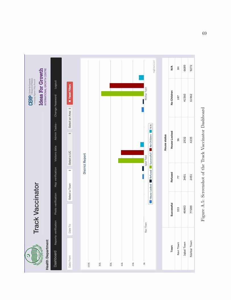
69

Fig

ure

A.5

:Scr

eensh

otof

the

Tra

ckV

acci

nat

orD

ashb

oard

70

010

2030

4050

Perc

ent

0 .1 .2 .3 .4 .5 .6 .7 .8 .9 1Average Proportion of Drive 1 Targets Completed

Figure A.6: Individual Completion Rates

71

Figure A.7: Drive 1 Vaccination Activity

Notes: The solid light grey circles are the share of all vaccination attempts that reflect a successful vaccination during the indicatedhour. The hollow dark black circles are the share of all vaccination attempts that report no children being available during theattempt. These quantities are compared against the left axis. The dotted line indicates the total number of vaccination attemptsfor all vaccinators in the sample. This quantity is compared against the right axis.

7211

012

013

014

015

016

0

Vacc

inat

ions

Allo

cate

d to

Soo

ner W

ork

Dat

ev_

1

.9 1 1.1 1.2 1.3R

Panel A: Drive 1Full Sample

110

120

130

140

150

160

Vacc

inat

ions

Allo

cate

d to

Soo

ner W

ork

Dat

ev_

1

.9 1 1.1 1.2 1.3R

Panel B: Drive 1Tailoring Sample

Advance Choice Immediate ChoiceAdvance Prediction Immediate Prediction

Figure A.8: Predicted and Actual Experimental ResponseNotes: Points in the plots are medians for each of the eight treatment groups respectively. Panel A depicts the Full Sample andPanel B depicts the tailoring sample (vaccinators with R∗ < 0.75 or R∗ > 1.5). Black are advance choice groups and gray areimmediate choice groups. The series for predictions correspond to Table 3, column (2).

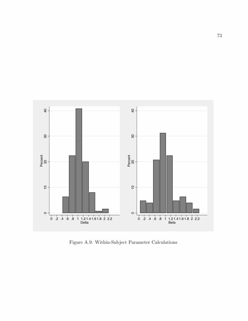
73

010

2030

40Percent

0 .2 .4 .6 .8 1 1.2 1.4 1.6 1.8 2 2.2Delta

010

2030

40Percent

0 .2 .4 .6 .8 1 1.2 1.4 1.6 1.8 2 2.2Beta

Figure A.9: Within-Subject Parameter Calculations

74

●

●●

●

●

● ●●

●

●

●

●

●

●

●

●●

●

●

●

●●

●

●

●

●●

●

●

●●

●

●

● ●

●

●

●

● ●

●

●●

●●●

●

●

●

●● ●

●

●●

●

●●

●

●

●

●●

●

●●

●

●

●

●

●

●

●

●●

●

●

●

●

●●

●

●

●●

●

●●

●

●

●●

●

●

●

●

●

●●

●●●

●●

●

●

●

●

●

●●

●

●

●

●

●●

●

●

●

●● ●

●

●●

●●

●

●

●●

●●

●●

●

●●●

●

●

●

●

●●●

●

●●

●● ●

●●●

●

●

●

●

●●

●●

●●

●

●

●

●

●●

●

●

●

●

● ●

●

●●

●

●

●

●

●●

●

●

●

●

●●●

●

●

●●

●

●●

●

●● ●

●

●●

●

●

●● ●

●

●

●

●●

●

●

●●

●

●

●

●

●

●

● ●

●

●●

●

●

●

●

●

●

●

●

●

●●●

●●●

●

●●

●

●

●●

●

● ●

●

●●

●

●●●

●

●

●●

●●● ●●

●

●

●

●●

●

●

●

●●

●

●

●●

●

●●

●

●

●

●

●●

●

●

●

●

●

●

●●●

●● ●

●

●

●

●

●

●●

●

●● ●●

●

60 80 100 120 140 160 180 200

6080

100

120

140

160

180

200

Actual

Pre

dict

ed

●

●●

●

●● ●

●

●

●

●

●

●

●

●●

●

●

●

●

●

●

●

●

●

●

●

●

●

●

●

●●

●●

●

● ●

●

●●

●●

●●

●

●

●

●

●

●●

●

●

●

●

●●

●

●

●

●

●

●

●

●

●

●

●

●

●

●

●

●

●

●

●

●●

●

●

●

●

●

●

●

●

●

●

●

●

●

●

●

●

●

●

●

●

●

●●

●

●

●

●

●

●

●

●

●

●

●

●

●

●●

●

●

●

●

●

●

●

●

●

●

●

●

●

●

●

●

●

●

●

●

●

●●

●

●

●

●

●

●

●

●●

●

●

●

●

●

●

●

●

●

●

●

●

●

●●

●

●

●

●

●

●●

●

●

●

●

●

● ●

●

●●

●

●

●

●

●

●

●

●

●

●

●

●

●

●●

●

●

●

● ●

●

●

●

●

●

●

●

●

●

●

●

●

●

●

●

●

●

●

●

●

●

●

●

●

●●

●

● ●

●

●

●

●

●

●

●

●

●

●

●

●

●

●

●

●

●

●

●

●

●

●

●

●

●

●

●

●

●

●

●

●

●

●●

●

●

●

●

●

●

●●

●

●

●

●

●

●

●

●

●

●

●

●

●

●

●

●

●

●

●

●

●

●

●

●

●

●

●

●

●

●

●

●

●

●

●

●

●

●

●●

●

●

●

●

●

●

●

●●

●

●

StructuralNon−Structural CV Lasso

Figure A.10: Structural and Non-Structural PredictionNotes: Predicted and actual Drive 2 value of v1 for structural and non-structural models. Structural prediction based on individualdiscount factor calculated from Drive 1. Non-structural prediction based on lasso regression of v1 on cubic polynomial in Rinteracted with 1d=1 from Drive 1. Lowess curves for non-parametric adherence to 45-degree line of perfect prediction.

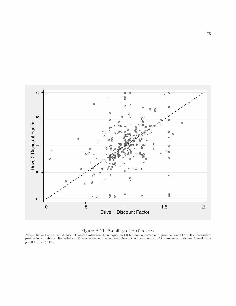
750

.51

1.5

2D

rive

2 D

isco

unt F

acto

r

0 .5 1 1.5 2Drive 1 Discount Factor

Figure A.11: Stability of PreferencesNotes: Drive 1 and Drive 2 discount factors calculated from equation (4) for each allocation. Figure includes 317 of 337 vaccinatorspresent in both drives. Excluded are 20 vaccinators with calculated discount factors in excess of 2 in one or both drives. Correlation:ρ = 0.41, (p < 0.01).

76

A.2 Appendix Tables

Table A.1: No Allocation Provided in Drive 0

Allocation Provided No Allocation Provided p-value(1) (2) (3)

Gender (Female = 1) 0.965 1.000 0.082(0.020) (0.000)

Years of Education 10.294 10.146 0.608(0.220) (0.185)

Number of Children 3.268 3.388 0.695(0.239) (0.188)

Punjabi (=1) 0.952 0.975 0.440(0.023) (0.018)

Has a Savings Account (=1) 0.317 0.305 0.867(0.052) (0.051)

Participated in a Rosca (=1) 0.446 0.378 0.380(0.055) (0.054)

Years in Health Department 10.135 10.886 0.337(0.554) (0.547)

Years as Polio Vaccinator 9.994 10.531 0.467(0.538) (0.502)

# Vaccinators 86 82

Notes: This table tests whether the failure of the smartphone app during Drive 0 was systematic. Standarderrors reported in parentheses. Column 3 reports a p-value corresponding to the null that the mean in theDid Not Fail group is equal to the Failed group.

77

Table A.2: Aggregate Drive 0 and 1 Behavior

Dependent variable: Tasks Allocated to the First Day of the Drive (v1)

Full Sample Tailoring Sample

(1) (2)Median Median

Immediate Decision (=1) -2.00** -3.00***(0.95) (0.88)

Interest Rate (R) -40.00*** -60.00***(6.04) (4.12)

Constant 188.00*** 210.00***(6.06) (4.34)

Median Advance Choice 150 150# Observations 622 475

Notes: This table reports on the effects of making Immediate allocation decisions and interestrate on Drive 0 and Drive 1 vaccinations allocated to the first day of the drive. Median regressioncoefficients with standard errors reported in parentheses. Standard errors are clustered at thevaccinator level. Clustered standard errors for quantile regressions are calculated using theapproach in Parente and Santos Silva (2016). Immediate Decision is an indicator equal to onefor vaccinators selecting their allocations on the morning of the vaccination drive. The interestrate R takes the values R ∈ {0.9, 1, 1.1, 1.25}. Levels of Significance: *p < 0.1, **p < 0.05,***p < 0.01.

Table A.3: Within Subject Parameter Estimates

(1) (2) (3) (4) (5) (6) (7) (8)All Panel Panel Panel

Observations Only No Change Change

β 0.895 0.903 0.930 0.931 0.946 0.944 0.906 0.912(0.030) (0.030) (0.032) (0.032) (0.048) (0.048) (0.043) (0.042)

δ 0.979 0.979 0.988 0.988 0.967 0.967 1.012 1.010(0.017) (0.017) (0.016) (0.016) (0.023) (0.023) (0.023) (0.023)

α 0.003 0.002 0.003 0.002(0.000) (0.000) (0.000) (0.000)

H0 : β = 1. (χ2(1)) 12.375 10.571 4.624 4.497 1.283 1.399 4.895 4.344[p-value] [0.000] [0.001] [0.032] [0.034] [0.257] [0.237] [0.027] [0.037]

Criterion Value 0.182 0.191 0.198 0.200 0.175 0.177 0.217 0.221# Observations 622 622 464 464 212 212 252 252# Vaccinators 390 390 232 232 106 106 126 126

Notes: This reports structural estimates of β, δ, and α obtained using minimum distance estimation of equations(1) in even columns or (2) and (3) in odd columns. Estimates provided for either all possible observations or panelof individuals participating in both Failed Drive 0 and Drive 1. Only Drive 1 data used for estimation of completionparameter, α. Standard errors clustered on individual level are reported in parentheses. Test statistic for β = 1 withp-value in brackets.

78

Table A.4: Additional Discounting Measures

Dependent variable: Drive 2 Allocation to Sooner Date v1,i

Untailored Tailored(1) (2) (3) (4)

Drive 0 Prediction 0.339* 0.203** 0.009 -0.017(0.174) (0.081) (0.066) (0.068)

Drive 1 Prediction -0.108 -0.051 0.406* 0.701***(0.187) (0.137) (0.212) (0.182)

Constant 109.010*** 122.367*** 83.530*** 43.805**(13.592) (14.128) (24.742) (20.610)

# Vaccinators 52 42 53 46Tailoring Sample No Yes No YesR-Squared 0.275 0.165 0.166 0.362R-Squared (Drive 0 Prediction Alone) 0.262 0.162 0.103 0.175R-Squared (Drive 1 Prediction Alone) 0.037 0.070 0.166 0.361

Notes: This table reports regressions for Drive 2 allocation on Drive 0 or Drive 1 predicted allocation forpanel of 105 individuals that remain in either Advance or Immediate choice across Drives 0 and 1. Predictedallocation from equation (4) individual discount factor. Heteroskedasticity robust White standard errorsreported in parentheses. *p < 0.1, **p < 0.05, ***p < 0.01.

79

Table A.5: Testing Stationarity of Costs Across Days

Panel A: Time Lapse Between Vaccinations (in minutes)

Dependent variable: Day 1 Med. Time Lapse Day 2 Med. Time Lapse Day 1 - Day 2 Med. Time Lapse(1) (2) (3) (4) (5) (6) (7) (8)

Advance Choice (=1) 0.519 1.134 1.011 -0.910 -1.161 -0.829 2.295 1.840(2.492) (1.163) (1.045) (3.164) (3.324) (3.182) (3.527) (3.343)

Discount Factor -3.697 10.004 -13.701(3.504) (8.247) (9.000)

Constant 3.370* 1.422*** 5.337 4.447* 4.540* -6.053 -3.118 11.390(1.851) (0.084) (3.708) (2.372) (2.501) (6.558) (2.501) (7.581)

R-Squared 0.000 0.004 0.016 0.000 0.001 0.013 0.002 0.022# Observations 265 228 228 240 228 228 228 228

Panel B: Distance Walked Between Vaccinations (in Kilometers)

Dependent variable: Day 1 Med. Distance Day 2 Med. Distance Day 1 - Day 2 Med. Distance(1) (2) (3) (4) (5) (6) (7) (8)

Advance Choice (=1) 0.112 0.146 0.132 -0.148 -0.171 -0.154 0.317 0.286(0.144) (0.154) (0.139) (0.152) (0.161) (0.144) (0.223) (0.199)

Discount Factor -0.444 0.509 -0.953(0.466) (0.516) (0.697)

Constant 0.059** 0.038*** 0.507 0.201 0.201 -0.337 -0.164 0.844(0.026) (0.010) (0.492) (0.151) (0.161) (0.388) (0.162) (0.629)


Notes: This table reports on the relationship between decision timing and the one period discount factor with two proxies of thecost of performing a vaccination (the amount of time that lapses between vaccinations and the distance traveled between vaccinations).Heteroskedasticity robust White standard errors reported in parentheses. *p < 0.1, **p < 0.05, ***p < 0.01.

80

Table A.6: Testing for Idiosyncratic Shocks

Panel A: Maximum Daily Time Lapse Between Vaccinations (in Minutes)

Dependent variable: Max Day 1 Time Lapse Max Day 2 Time Lapse Day 1 - Day 2 Max Time Lapse(1) (2) (3) (4) (5) (6) (7) (8)

Advance Choice (=1) -0.702 0.578 0.739 8.067 5.274 5.574 -4.695 -4.836(9.783) (9.104) (9.026) (8.885) (9.114) (9.021) (12.319) (12.211)

Discount Factor 4.831 9.054 -4.223(14.139) (15.570) (19.824)

Constant 59.258*** 54.880*** 49.764*** 53.437*** 54.362*** 44.774*** 0.518 4.990(7.920) (7.254) (15.266) (5.178) (5.404) (15.351) (8.724) (20.662)


Panel B: Maximum Time Lapse > 2 hours

Dependent variable: Max Day 1 Lapse > 2hr. Max Day 2 Time Lapse > 2hr. Day 1 > 2hr. - Day 2 > 2hr.(1) (2) (3) (4) (5) (6) (7) (8)

Advance Choice (=1) 0.051 0.042 0.044 0.026 0.001 0.002 0.041 0.042(0.045) (0.047) (0.047) (0.041) (0.042) (0.041) (0.060) (0.060)

Discount Factor 0.053 0.032 0.021(0.077) (0.071) (0.100)

Constant 0.133*** 0.127*** 0.071 0.103*** 0.109*** 0.075 0.018 -0.004(0.029) (0.032) (0.085) (0.028) (0.030) (0.075) (0.043) (0.111)


Notes: This table reports on the relationship between decision timing and the one period discount factor with two proxies for experiencing a shock duringthe drive (the maximum time lapse between vaccinations and whether a lapse of more than 2 hours occurred). Heteroskedasticity robust White standarderrors reported in parentheses. *p < 0.1, **p < 0.05, ***p < 0.01.

Table A.7: Aggregate Parameter Estimates, Alternate Probabilistic Completion

(1) (2) (3) (4) (5) (6) (7) (8)γ = 2 γ = 2.5 γ = 3 γ = 3.25

p(v1, v2) = 11+α′(v21+v22)

11+α′′(v31+v32)

11+α′(v21+v22)

11+α′′(v31+v32)

11+α′(v21+v22)

11+α′′(v31+v32)

11+α′(v21+v22)

11+α′′(v31+v32)

β 0.944 0.936 0.935 0.924 0.924 0.910 0.917 0.883(0.030) (0.030) (0.040) (0.039) (0.050) (0.050) (0.055) (0.053)

δ 0.992 0.992 0.967 0.966 0.943 0.942 0.931 0.926(0.017) (0.017) (0.022) (0.022) (0.027) (0.027) (0.030) (0.028)

α′ 0.000022 0.000022 0.000022 0.000022(0.000002) (0.000002) (0.000002) (0.000002)

α′′ 1.48e−7 1.50e−7 1.50e−7 6.58(1.63e−8) (1.64e−8) (1.65e−8) (.)

H0 : β = 1. (χ2(1)) 3.583 4.650 2.700 3.681 2.341 3.299 2.261 4.904[p-value] [0.058] [0.031] [0.100] [0.055] [0.126] [0.069] [0.133] [0.027]


Notes: This reports structural estimates of β, δ, and α obtained using minimum distance estimation of equations (1) in even columns or (2) and(3) in odd columns. Standard errors are reported in parentheses. Test statistic for β = 1 with p-value in brackets.

81

Table A.8: Aggregate Parameter Estimates, Alternate Net Completion Utility

(1) (2) (3) (4) (5) (6) (7) (8)γ = 2 γ = 2.5 γ = 3 γ = 3.25

[δ2u(1000)− vγ1 − β1d=1δ · vγ2 ] = 1000 10000 1000 10000 1000 10000 1000 10000

β 0.952 0.952 0.946 0.946 0.938 0.940 0.934 0.906(0.029) (0.029) (0.039) (0.039) (0.050) (0.050) (0.055) (0.053)

δ 0.992 0.996 0.967 0.967 0.942 0.943 0.931 0.915(0.017) (0.017) (0.022) (0.022) (0.027) (0.027) (0.030) (0.029)

α 0.003 0.003 0.003 0.003 0.003 0.003 0.003 -0.016(0.000) (0.000) (0.000) (0.000) (0.000) (0.000) (0.000) (0.000)

H0 : β = 1. (χ2(1)) 2.644 2.710 1.856 1.855 1.525 1.466 1.425 3.070[p-value] [0.104] [0.100] [0.173] [0.173] [0.217] [0.226] [0.233] [0.080]


Notes: This reports structural estimates of β, δ, and α obtained using minimum distance estimation of equations (1) in evencolumns or (2) and (3) in odd columns. Standard errors are reported in parentheses. Test statistic for β = 1 with p-value inbrackets.

Table A.9: Tailoring with Alternative Controls


v2,i− 1|

Comparison group: Untailored with Untailored with Untailored with

Ri ∈ +/− 1 s.d of Mean R∗i Ri ∈ +/− 1 s.d of Mean R∗i Matched Distribution of Ri

|R∗i − Ri| > 0.10

(1) (2) (3)

Tailored (=1) -0.039* -0.052** -0.047**(0.021) (0.025) (0.022)

Constant 0.200*** 0.231*** 0.085(0.071) (0.074) (0.072)

Stratum FEs Yes Yes YesExclude 99th and 1st Percentiles Yes Yes Yes

Drive 2 R∗i or Ri Yes Yes Yes

R-Squared 0.081 0.086 0.071Mean in Untailored Contract 0.132 0.150 0.143# Vaccinators 194 181 207# Untailored Vaccinators 59 46 72

Notes: This table reports the effects of tailoring on the equality of effort provision over time. The measure | vtvt+1− 1| (the percentage difference

between tasks allocated to day 1 and day 2 of the drive) reflects the distance of the task allocation (v1,v2) from equality (v1 = v2). Mean (standarddeviation) R∗

i in untailored group = 1.036 (0.165). Heteroskedasticity robust White standard errors reported in parentheses. *p < 0.1, **p < 0.05,***p < 0.01.

82

Table A.10: Tailoring and Completion


v2,i− 1|

(1) (2) (3) (4) (5) (6)Completed Drive 1 Failed Drive 1

Tailored (=1) -0.031 -0.055** -0.042* -0.977 -0.075** -0.065**(0.039) (0.025) (0.024) (0.652) (0.030) (0.029)

Constant 0.100*** 0.114*** -0.051 1.967 0.181*** 0.032(0.037) (0.032) (0.088) (1.222) (0.030) (0.079)

Stratum FEs Yes Yes Yes Yes Yes YesExclude 99th and 1st Percentiles No Yes Yes No Yes Yes

Drive 2 R∗i or Ri No No Yes No No Yes

R-Squared 0.051 0.095 0.130 0.045 0.053 0.078Mean in Untailored Contract 0.151 0.129 0.129 1.161 0.183 0.183# Vaccinators 147 142 142 133 125 125

Notes: This table reports the effects of tailoring on the equality of effort provision over time. The measure | vtvt+1−1|

(the percentage difference between tasks allocated to day 1 and day 2 of the drive) reflects the distance of the taskallocation (v1,v2) from equality (v1 = v2). Column (1) reports a regression of this measure on an indicator equalto one for subjects in the tailored group. Column (2) reports estimates from the same specification excludingoutliers. Column (3) controls for the interest rate assignment in round 2. Column (4) provides estimates on thesame sample as column (1) interacting treatment with being in the immediate choice condition. Columns (5) and(6) apply the same restrictions to the sample as columns (2) and (3) respectively. Ordinary least squares regressions.Heteroskedasticity robust White standard errors reported in parentheses. *p < 0.1, **p < 0.05, ***p < 0.01.

83

Table A.11: Robustness Tests for Tailoring Intertemporal Incentives

Panel A: Dependent variable|v1,i−v2,i|√

2

(1) (2) (3) (4) (5) (6)

Tailored (=1) -1.758 -4.480** -4.481** -2.401 -1.703 -1.868(4.588) (1.954) (2.068) (2.302) (2.176) (2.229)

Immediate Choice 20.994*** 10.365*** 10.597***(5.856) (3.335) (3.449)

Tailored x Immediate 2.127 -6.026 -6.220(9.793) (4.084) (4.136)

Constant 31.386*** 16.399*** 16.412** 19.464*** 10.992*** 14.128**(7.334) (2.296) (6.857) (6.433) (2.777) (6.671)

Panel B: Dependent variable|v1,i−v2,i|√2(v1,i+v2,i)

(1) (2) (3) (4) (5) (6)

Tailored (=1) -0.014 -0.018*** -0.016** -0.009 -0.007 -0.007(0.015) (0.007) (0.007) (0.008) (0.007) (0.008)


Tailored x Immediate -0.008 -0.024* -0.023*(0.032) (0.014) (0.014)

Constant 0.103*** 0.057*** 0.033 0.058*** 0.037*** 0.025(0.023) (0.008) (0.022) (0.020) (0.010) (0.022)

Panel C: Dependent variable |v1,i − 3001+R|

(1) (2) (3) (4) (5) (6)

Tailored (=1) -2.612 -3.789*** -3.445** -1.959 -1.509 -1.405(3.282) (1.410) (1.459) (1.643) (1.575) (1.591)


Tailored x Immediate -0.867 -4.972* -4.850(6.891) (2.938) (2.974)

Constant 22.736*** 12.014*** 7.571 13.340*** 7.849*** 5.871(5.301) (1.682) (4.735) (4.501) (2.048) (4.622)

Panel D: Dependent variable |v1,i − 3001+R| > 25

(1) (2) (3) (4) (5) (6)

Tailored (=1) -0.454** -0.654*** -0.578*** -0.282 -0.282 -0.235(0.191) (0.221) (0.216) (0.317) (0.314) (0.309)

Immediate Choice 0.920*** 0.720** 0.697**(0.272) (0.283) (0.286)

Tailored x Immediate -0.275 -0.676 -0.653(0.408) (0.462) (0.460)

Constant -0.639*** -0.887*** -1.568** -1.231*** -1.312*** -1.812***(0.206) (0.239) (0.637) (0.304) (0.335) (0.665)

Panel E: Dependent variable min[v1,i, v2,i]

(1) (2) (3) (4) (5) (6)

Tailored (=1) 7.210** 8.112*** 2.540* 4.764* 4.381* 0.843(3.512) (2.051) (1.416) (2.650) (2.643) (1.567)

Immediate Choice -20.562*** -11.804*** -6.815***(5.042) (3.492) (2.332)

Tailored x Immediate 4.672 8.194** 4.037(7.206) (4.052) (2.806)

Constant 126.824*** 136.728*** 208.758*** 138.343*** 142.870*** 210.228***(5.181) (2.645) (4.541) (4.905) (3.359) (4.433)

Stratum FEs Yes Yes Yes Yes Yes YesExclude 99th and 1st Percentiles No Yes Yes No Yes YesDrive 2 R No No Yes No No Yes# Vaccinators 280 267 267 280 267 267

Notes: This table reports the effects of tailoring on the equality of effort provision over time using several different measures of thedistance of the task allocation (v1,v2) from equality (v1 = v2). Column (1) reports a regression of this measure on an indicator equalto one for subjects in the tailored group. Column (1) reports a regression of this measure on an indicator equal to one for subjects inthe tailored group. Column (2) reports estimates from the same specification excluding outliers. Column (3) controls for the interestrate assignment in round 2. Column (4) provides estimates on the same sample as column (1) interacting treatment with being inthe immediate choice condition. Columns (5) and (6) apply the same restrictions to the sample as columns (2) and (3) respectively.Heteroskedasticity robust White standard errors reported in parentheses. *p < 0.1, **p < 0.05, ***p < 0.01.

84

Table A.12: Alternate Treatment Measures and Sample Restrictions

Panel A: Tailoring Intensity


v2,i− 1|

(1) (2) (3) (4) (5) (6)

Tailor Intensity 2.521 0.164** 0.110* 0.078 0.124 0.089(2.057) (0.065) (0.063) (0.188) (0.081) (0.076)

Immediate Choice -0.065 0.071*** 0.068***(0.312) (0.023) (0.022)

Tailor Intensity x Immediate 4.537 0.071 0.057(3.809) (0.133) (0.131)

Constant 0.780* 0.104*** -0.009 0.765 0.067*** -0.018(0.457) (0.018) (0.058) (0.482) (0.020) (0.058)

# Vaccinators 280 267 267 280 267 267

Panel B: Tailoring Intensity and Boundary Sample


v2,i− 1|

(1) (2) (3) (4) (5) (6)

Tailor Intensity 1.200 0.151** 0.124* -0.038 0.054 0.025(1.006) (0.069) (0.065) (0.127) (0.060) (0.054)

Immediate Choice 0.094 0.066*** 0.064**(0.202) (0.025) (0.025)

Tailor Intensity x Immediate 2.075 0.148 0.154(1.848) (0.119) (0.114)

Constant 0.712* 0.152*** 0.044 0.652* 0.119*** 0.016(0.368) (0.026) (0.065) (0.369) (0.026) (0.063)

# Vaccinators 337 320 320 337 320 320

Stratum FEs Yes Yes Yes Yes Yes YesExclude 99th and 1st Percentiles No Yes Yes No Yes YesDrive 2 R No No Yes No No Yes

Notes: This table reports the effects of tailoring on the equality of effort provision over time. The measure| vtvt+1

− 1| reflects the distance of the task allocation (v1,v2) from equality (v1 = v2). Column (1) reports a

regression of this measure on an indicator equal to one for subjects in the tailored group. Column (2) reportsestimates from the same specification excluding outliers. Column (3) controls for the interest rate assignment inround 2. Column (4) provides estimates on the same sample as column (1) interacting treatment with being in theimmediate choice condition. Columns (5) and (6) apply the same restrictions to the sample as columns (2) and(3) respectively. Heteroskedasticity robust White standard errors reported in parentheses. *p < 0.1, **p < 0.05,***p < 0.01.report*p < 0.1, **p < 0.05, ***p < 0.01.

nber working paper series using …this paper seeks to understand whether the out-of-sample...

Documents