NBER WORKING PAPER SERIES

PRICING CAPITAL UNDER MANDATORY UNBUNDLINGAND FACILITIES SHARING

Robert S. Pindyck

Working Paper 11225http://www.nber.org/papers/w11225

NATIONAL BUREAU OF ECONOMIC RESEARCH1050 Massachusetts Avenue

Cambridge, MA 02138March 2005

This paper resulted in part from a study commissioned by Verizon Communications, Inc. The author thanksColeman Bazelon of Analysis Group, Inc. and Thomas Hazlett of the Manhattan Institute for their help withall aspects of this project, John Browning and Aaron Thegeya, both of Analysis Group, Inc., for theiroutstanding research assistance, and Jerry Hausman, Paul Joskow, and Stewart Myers for helpful discussions.The views expressed herein are those of the author(s) and do not necessarily reflect the views of the NationalBureau of Economic Research.

©2005 by Robert S. Pindyck. All rights reserved. Short sections of text, not to exceed two paragraphs, maybe quoted without explicit permission provided that full credit, including © notice, is given to the source.

Pricing Capital Under Mandatory Unbundling and Facilities SharingRobert S. PindyckNBER Working Paper No. 11225March 2005JEL No. L51

ABSTRACT

The regulation of telecommunications, railroads, and other network industries has been based on

mandatory unbundling and facilities sharing - entrants have the option to lease part or all of

incumbents' facilities if and when they desire, at rates determined by regulators. This flexibility is

of great value to entrants, but because investments are largely irreversible, it is costly to supply by

incumbents. However, pricing formulas used by regulators to set lease rates for capital do not

compensate incumbents for this flexibility, so that incumbents are effectively forced to subsidized

entrants, discouraging further investments. This paper shows how pricing formulas used to set lease

rates can be adjusted to account for the transfer of option value from incumbents to entrants, and

estimates the average size of the adjustment for land-based local voice telecommunications in the

U.S.

Robert S. PindyckSloan School of ManagementMIT, Room E52-45350 Memorial DriveCambridge, MA 02139and NBERrpindyck@mit.edu

1

1. Introduction.

With the goal of increasing competition, the Telecommunications Act of 1996 allowed

entrants to use incumbents’ telephone networks according to terms and conditions determined by

regulators. The requirement that network owners share parts or all of their capital with rivals is

referred to as mandatory unbundling. Entrants have the option to lease incumbents’ facilities if

and when they desire, for services of their choosing. This flexibility is of great value to entrants,

but because network investments are largely irreversible, it is costly to supply by incumbents.

However, the pricing formula used by regulators to set lease rates for capital (i.e., wholesale

prices for access to network infrastructure) does not compensate incumbents for the flexibility

granted to entrants. The result is that wholesale network prices are set below competitive levels,

so that incumbents are effectively forced to subsidize entrants, discouraging further investments.

The goal of this paper is to show how the pricing formula used to set lease rates can be adjusted

to account for the transfer of “option value” from incumbents to entrants.

Telecom regulation in the U.S. is currently in transition. The Telecom Act’s unbundling

requirements were challenged in the courts, and on May 24, 2004, they were struck down by a

federal appeals court.1 The Federal Communications Commission will thus have to design a new

regulatory framework to replace the original unbundling requirements. The current pricing

formula used to set lease rates was previously upheld by the Courts, but may be abandoned by

federal regulators.2 State regulatory agencies may have to follow suit. But whatever happens to

telecom regulation in the U.S., the problem of capital pricing under mandatory unbundling

regimes remains important. This regulatory framework has been and continues to be applied to

other industries in the U.S., as well as to telecom and other industries outside of the U.S.3

1 On October 12, 2004, the U.S. Supreme Court declined to hear the appeal of that decision. 2 The Supreme Court upheld the current approach to pricing (TELRIC) on May 13, 2002. On Dec. 15, 2004, the FCC relaxed, but did not eliminate, rules requiring the former Bell companies to give entrants access to their networks at sharply discounted rates. 3 Mandatory unbundling has been used in the regulation of U.S. railroads, and as Hausman and Myers (2002) discuss, regulated capital prices ignore the transfer of option value. Mandatory unbundling has been proposed for U.S. electricity markets. Local loop unbundling has been implemented in much of the OECD. By April, 2002, 23 of the 30 OECD countries had legislated some form of unbundling. (See “Developments in Local Loop Unbundling,” September 10, 2003, OECD, p. 15; at http://www.oecd.org/dataoecd/25/24/6869228.pdf, visited Sept. 14, 2004.) For example, European Commission Regulation No. 2887/2000, effective January 2, 2001, specifies that incumbent local telecom companies must make available the unbundled access to their subscriber connections and the attached facilities (see http://www.tkc.at/publikationen/tkbericht2000/en/2/2321.htm, visited Sept. 14, 2004).

2

The basic problem with mandatory unbundling and sharing as applied in practice is that the

pricing of capital generally ignores the irreversible (i.e., sunk cost) nature of most of the relevant

investments. In the case of the Telecom Act, pricing is based on a framework called Total

Element Long Run Incremental Costs, or TELRIC.4 The idea is to set the rental rate for each

network element equal to the incremental cost of creating and supplying that leased element if

the network owner were designing and constructing a completely new, optimally configured

network with state-of-the-art technology. But TELRIC pricing under-compensates incumbents

for their investments because of its treatment of risk.5 When making an irreversible investment,

an incumbent sees the opportunity for positive returns in “good times” as compensation for

losses should “bad times” prevail, and thus should require a hurdle rate for the investment that is

higher than its cost of capital. An entrant, however, does not have this same exposure to risk. If

market conditions are favorable, the entrant will lease equipment, but if conditions are

unfavorable, it will not. Thus, unlike the incumbent that actually made the capital investment,

the entrant does not bear the burden of the uncertainty – it benefits on the upside, while avoiding

the downside. In effect, the entrant is granted an option to enter or exit at will. The TELRIC

price, however, does not take the value of this option into account, and therefore under-

compensates the incumbent – discouraging capital investment.6

Why is it important that these regulated prices account for the full economic value of the

capital? Putting aside issues of equity, the main reason is that a regulatory regime that

systematically under-compensates incumbents will discourage future capital investment, which

in the long run will harm consumers.

It has been argued that in the case of telecommunications and railroads, this is not a problem

because the capital has already been sunk. Indeed, if no new investment were needed to

maintain or improve existing communications networks, the disincentives resulting from policies

4 I am focusing here on wholesale prices. Retail prices for incumbents are usually subject to price-cap or rate of return regulation set on a state-by-state basis. A few states, such as Massachusetts, have deregulated or allowed increased pricing flexibility for the rates that incumbent ILECs can charge retail customers. 5 TELRIC also under-compensates incumbents because of its use of “forward looking costs,” i.e., it sets rental rates based on current or expected future equipment costs, rather than the historical costs that the incumbent actually paid for the equipment. Because equipment costs tend to fall over time, incumbents will not recover their sunk costs. I do not address this problem here, but it is discussed in Pindyck (2004) and Salinger (1998). 6 The fact that TELRIC does not compensate incumbents for their transfer of option value to entrants has been pointed out by Hausman (1997, 2003). The problem and its implications for investment in telecom networks are also discussed in Pindyck (2004). For a related analyses, see Kotakorpi (2004) and Bourreau and Dogan (2005).

3

that under-compensate investors might not be of much importance (unless those policies

increased the risk of bankruptcy). Owners of existing facilities would suffer economic losses,

but consumers would be largely unaffected, because earlier investments in the existing networks

cannot be “undone.” Telecom networks, however, require ongoing investments just to maintain

a given quality of service, and companies have discretion over the timing of those investments

and over the extent to which quality is maintained or improved.7 A related claim is that

investment incentives are unimportant because incumbents have a “duty to serve,” i.e., they must

provide service to any customer requesting it, and therefore must invest accordingly. But the

duty to serve is a limited obligation that only applies to basic service, not ancillary services such

as call waiting, three-way calling, etc., and does not address all aspects of the quality of service.

Again, companies have discretion over much of their investment.

It has also been argued that regulatory regimes based on mandatory unbundling and the

sharing of incumbents’ facilities are inherently flawed, and are very unlikely to generate long-run

welfare gains for consumers.8 In the case of the 1996 Telecom Act, mandatory unbundling

became a significant reality starting only around 1999, so it is difficult to empirically assess its

impact on prices, quality of service, and investment, although a number of studies have tried to

do so.9 This paper is not concerned with that debate, and takes mandatory unbundling as a given.

Regulatory authorities have adopted mandatory unbundling and facilities sharing as a means of

generating competition, so even as a second-best policy, it is important to implement it

optimally. This means pricing shared capital correctly, and in particular, accounting for the

irreversibility of investment and the transfer of option value that it implies.

I address the pricing of unbundled network elements (UNEs) in telecommunications

7 From 1990 to 1995, approximately $20 billion in annual capital expenditures was used just to maintain existing Bell networks, and further investments are necessary to upgrade systems or to deploy new technologies. With demand for data services (including DSL) beginning to drive new capital expenditures starting around 1996, annual investment grew strongly through 2000. By 2002, real ILEC investment had fallen to about where it was in 1990, and investment continued to fall in 2003. As discussed in Pindyck (2004), substantial expenditures are needed simply to maintain the existing infrastructure. See Hausman and Myers (2002) for a discussion of this point in the context of railroads. 8 See, e.g., Kahn (2004) and Tardiff (1999), and for empirical evidence, Hausman and Sidak (2005). 9 Studies that show overall gains from mandatory unbundling include Clarke et. al. (2004), Willig et al. (2002), Ford and Pelcovits (2002) and Phoenix Center (2003). Studies that show reduced investment and thus losses include Jorde, Sidak, and Teece (2000), Crandall, Ingraham, and Singer (2004), and Hazlett, Havenner, and Bazelon (2003). Focusing on the demand side of the market, Economides, Seim, and Viard (2004) estimate the consumer welfare benefits of entry into local markets following the 1996 Telecom Act. Knittel (2004) estimates price impacts, and Greenstein and Mazzeo (2003) show that entrants seem to differentiate their services, and thereby provide variety.

4

networks, and show how the TELRIC framework can be corrected to account for the transfer of

option value from incumbent local exchange carriers (ILECs) to entrants, i.e., competitive local

exchange carriers (CLECs). The recent policy debate over TELRIC has raised two important

questions:

1. How should the transfer of option value be taken into account, i.e., how should

TELRIC be adjusted?

2. How significant is this transfer of option value, i.e., as a practical matter is it

important to take it into account?

This paper attempts to answer both of these questions. Although I focus on telecommunications,

the results developed here can be applied to capital pricing under mandatory unbundling regimes

in other industries as well.

In the next section, I lay out a model of investment and pricing that accounts for the fact that

part of an incumbent’s investment is subject to a “duty to serve,” but part is discretionary. I then

show that while there are many ways to “fix” TELRIC, i.e., to adjust prices so that they include

option value, the simplest approach from the point of view of implementation is to adjust the cost

of capital input used in the current TELRIC formulation. I show that this adjustment can be

calculated from a small set of observable market variables, so that its use by federal or state

regulatory agencies should be reasonably straightforward. I calibrate the model using data on

capital stocks, prices, investment, and other variables for U.S. local exchange carriers, and then

estimate the size of the adjustment to the cost of capital needed to correct TELRIC. I find that

adjustment to be as high as 4.5 percentage points. For example, an ILEC’s roughly 13 percent

cost of capital would have to be increased to 17.5 percent when used as an input in TELRIC.

2. The Model.

I consider two kinds of capital, both of which are industry-specific and long-lived, and thus

can be treated as irreversible investments. The first kind is the basic line for residential or

business service. The ILEC must invest in this capital to meet demand, and the price of this

basic service is regulated.10 The second kind of capital is used to provide a variety of other

10 Regulated prices differ, however, for residential versus business service, and they also differ considerably from state to state. But as we will see, the specific levels of those regulated prices do not affect the magnitude of the correction to TELRIC.

5

services, the prices of which are unregulated. These include ancillary “vertical” services, such as

call waiting, three-way calling, voice mail, etc. (I will refer to all of these other unregulated

services as “ancillary services.”) The ILEC has discretion over the purchase and installation of

this capital, i.e., it has the option to install it if and when it wants. The demand for these

ancillary services depends on the price, which is unregulated. However, a customer can buy

ancillary services only if he or she has a telephone line, i.e., has basic service.

Under the 1996 Telecom Act’s mandatory unbundling rules, a CLEC can lease parts of the

network (i.e., one or more UNEs) from the ILEC and use them to provide both basic and

ancillary services. CLECs typically have little interest in providing basic service alone, because

the profit margins on such service are low or zero. Providing a customer with basic service,

however, gives the CLEC the ability to sell that customer the ancillary services for which

margins are higher. (CLECs usually target their marketing efforts toward potential customers

who – based on income or other characteristics – are likely to purchase ancillary services. In

fact, often CLECs will only offer potential customers a bundled service that includes the basic

line as well as the ancillary services.) Without loss of generality, I consider an ILEC that faces

entry by a single CLEC.

I assume that the demands for basic service and ancillary services fluctuate stochastically, so

that (for any given price) future demands are uncertain. I also assume that capital – whether

copper loops, switches, or central billing facilities – can be measured in “line-equivalents.” Thus

the provision of basic service to a residential customer requires one line-equivalent of capital,

and the provision of ancillary services to that customer requires an additional multiple (in

practice less than one) of a line-equivalent of capital. Consistent with the way that depreciation

is treated in the TELRIC framework, I also assume that capital lasts for a fixed period of time, T.

Based on an estimate by Vander Weide (2003), the average lifetime for LEC capital is about 14

years, although this number can vary depending on the specific type of capital.

The quantity of basic service demanded, measured in lines, is given by xt, which evolves

stochastically (see below). This service, which the ILEC has a duty to provide, is sold at the

regulated price P1. The second, higher-margin segment of demand is for ancillary “vertical”

services. The (inverse) demand curve for this segment is linear and is given by:

2 (t tP b x Q2 )t= − (1)

Here, Q2t is the number of lines for which ancillary services have been added. Note that for any

6

positive price P2t, , i.e., not all lines have ancillary services. The variable x2tQ x< t t, which shifts

the demand curve inwards or outwards, follows the Geometric Brownian Motion (GBM):

tdx axdt xdzσ= + (2)

where dz is the increment of a Wiener process. Later I discuss how the drift and volatility

parameters, a and σ, can be estimated.

Let K = K1 + K2 denote the ILEC’s total capital stock, measured in line-equivalents (LEs).

This capital stock has two components; K1 is the number of LEs used to provide basic service,

and K2 is the number used to provide ancillary services for a subset of the basic lines. Because xt

is measured in terms of the number of lines, K1 = xt. The capital needed to provide ancillary

services is proportional to the quantity of those services: 2K Q2γ= . I assume that the ILEC has

a constant per-line marginal cost, c1, of providing basic service, and a constant marginal cost, c2,

of providing ancillary services, and that these costs are the same for a CLEC. The cost of capital

for both the ILEC and the CLEC is rρ > , where r is the risk-free interest rate. Thus ρ is the

discount rate, adjusted for systematic risk, which the firms use to value future cash flows. In this

setting, ρ might be the firm’s weighted average cost of capital (WACC). I denote by k the cost of

one line-equivalent unit of capital, which I assume is constant.

In eqn. (2) for the demand shift variable, a is the drift rate, i.e., the expected rate of growth

of xt. The risk-adjusted expected rate of return associated with xt is ρ, so aδ ρ= − is the “return

shortfall” for xt. I assume that a ρ< (otherwise investments would yield infinite returns).

When the CLEC leases capital, it pays the ILEC the TELRIC price for each unit of capital

that it leases. The TELRIC price is the amortized cost of the unit, based on the ILEC’s cost of

capital, ρ. If capital lasted forever, i.e., if there were no depreciation, the TELRIC price would

simply be TA kρ= . If capital lasts for T years, the TELRIC price would be:11

(1 )(1 ) 1

T

T TA ρ ρρ+

= k+ −

(3)

11 E.g., for a WACC of 13% and an average lifetime of 14 years, AT = .159k. The details of TELRIC pricing are complicated (many individual costs must be estimated for specific network configurations), but the basic idea is straightforward: The ILEC is “reimbursed” for its capital cost through an annual WACC-based annuity payment. TELRIC also includes payment for one-time set-up costs and direct and indirect ongoing fixed costs, which I ignore.

7

Finally, to simplify the analysis of the firm’s investment decisions, I assume that all capacity

is utilized as long as marginal revenue from the last unit of capacity is positive. In other words, I

ignore the presence of “operating options” (i.e., options to leave some capacity unutilized if the

revenue from that capacity is below variable cost).12

2.1. ILEC Profit and Investment.

Let us assume for the time being that there is no entry by CLECs. The ILEC’s flow of

profit from the provision of basic service is then given by:

(4) 1 1 1( ) TP c x A xΠ = − −

I assume that the price of basic service is set so that the resulting economic profit is just zero,

i.e., . The variable profit from the provision of ancillary services, i.e., the profit

ignoring the cost of the capital needed to provide those services, is

1 1 TP c A= +

(5) 2 2 2( )tb x Q Q c QΠ = − − 2 2

2

Thus the incremental profit from the provision of ancillary services to one more customer is

(6) 2 22bx bQ c∆Π = − −

Since 2 2 /Q K γ= and , we can write ∆Π2K K= − x 2 in terms of the total capital stock K :

2( 2) 2( ; ) b bK x x K c2γγ γ+

∆Π = − − (7)

Assuming that the incremental unit of capital is always utilized (so that there are no

operating options), the value of the unit is the expected present value of this incremental flow of

profit over the lifetime of the capital:

( ) 22 2

( 2) 2( ; ) ( ; )t T

t T Tt t t

t

b D bD cV K x K x e d x Kρ ττ

γτ TDδγ ργ

+− − +

∆ = Ε ∆Π = − −∫ ρ (8)

where 1 TTD e ρ−≡ − is the depreciation factor, and recall that aδ ρ= − .

Now consider the ILEC’s decision to invest in this incremental unit of capital. We must find

the value of the option to invest in the unit, and the critical value of x that triggers that

investment. That critical value, x*(K), is a function of total capacity K, and can be inverted to

12 Operating options can be introduced at the cost of making the algebra messier. See Dixit and Pindyck (1994) and Pindyck (1988). Operating options are unlikely to matter much, however, because marginal cost is low. If demand is linear, as for this model, marginal revenue can in principle become negative if all capacity is always utilized. For reasonable parameterizations, however, that is unlikely, so I ignore that possibility.

8

yield the optimal capacity K*(x). The value of the option to invest in an incremental unit of

capacity for the provision of ancillary services, which I denote by 2 ( ; )F K x∆ , must satisfy the

following differential equation (see Pindyck (1988) and Dixit and Pindyck (1994)):

2

2 2 2 222

1 ( )2

F Fx r x r Fx x

σ δ∂ ∆ ∂∆ 0+ − − ∆∂ ∂

= (9)

along with the following three boundary conditions:

2 ( ,0) 0F K∆ = (10)

* *2 2( , ) ( , )F K x V K x kγ∆ = ∆ − (11)

* *

2 2( , ) ( , )F K x V K xx x

∂∆ ∂∆=

∂ ∂ (12)

Using boundary condition (10), the solution to this differential equation is given by:

2 ( , )F K x Bxβ∆ = (13)

for * *2 2, and ( , ) ( , ) for x x F K x V K x k xγ≤ ∆ = ∆ − > x , and where

2 2 22 2

1 ( ) 1 ( / 2) 22

r r 1rδβ δ σσ σ−

= − + − − + >σ (14)

There are still two unknowns, the constant B and the critical value x*. They can be found

from the remaining two boundary conditions (11) and (12). Substituting eqns. (13) and (8) into

those conditions yields the following expression for the critical value x*(K):

*2( ) (2 / )

1 ( 2) T2x K bK c

bβ δ γ γ ρ

β ρ γ⎛ ⎞

= + +⎜ ⎟− +⎝ ⎠k D (15)

This expression can be inverted to give the ILEC’s optimal capital stock:

*2

1 ( 2)( ) ( / )2 2 TK x x c k D

bβ ρ γ γ γρβ δ

⎛ ⎞− += − +⎜ ⎟⎝ ⎠

(16)

Finally, the solution for B is given by:

1

22

( 2) ( 1)( )2 /

T

T

D bB KbK c k D

ββγ ρ β

γ βδ γ γ ρ

−⎛ ⎞⎛ ⎞+ −

= ⎜⎜ ⎟ + +⎝ ⎠ ⎝ ⎠⎟ (17)

Note from eqn. (14) that an increase in the volatility of demand, σ, makes β smaller, so that

the optimal capital stock becomes smaller. And note from eqn. (17) that , so that other

things equal, the larger is K, the smaller is the value of the option to add one more unit of capital.

'( ) 0B K <

9

2.2. Correcting TELRIC.

Now suppose that a CLEC can lease this incremental unit of capital from the ILEC over

arbitrarily short periods of time at the annual TELRIC rental rate of AT per unit, with AT given by

eqn. (3). To provide ancillary services to the incremental customer, the CLEC must also provide

the customer with basic service, so that it will need (1 + γ) line-equivalents of capital, and will

incur an annual cost for this capital of (1 TAγ+ ) . The ILEC receives this annual payment, so

initially it earns zero economic profit. However, should x fall (i.e., market conditions become

adverse), the CLEC will stop leasing the capital, and the ILEC will have a negative economic

profit. Thus, the ILEC’s average return on the capital will be negative, and it will have no

incentive to make the investment needed to provide the incremental ancillary service. (I assume

that it has no choice with regard to its investment in the capital needed to provide basic service.)

The problem here is that the value of the ILEC’s option has been transferred to the CLEC,

but the CLEC’s rental rate under TELRIC does not account for this. To see this, note that under

the optimal exercise rule (and absent the CLEC), the ILEC’s net payoff when it invests is

(18) * *2 2( ; ) ( ; ) 0F K x V K x kγ∆ = ∆ − >

Under this optimal rule, the NPV of the investment is greater than zero because if market

conditions deteriorate, the ILEC will hold capital that it would prefer not to have. If it had no

option to choose the timing of its investment (or if, like the CLEC, it could freely “uninvest” in

the future), ∆F2 would be zero, and investment would occur at the point where 2V kγ∆ = .

Under TELRIC, this option is transferred to the CLEC, so the full economic value of the

capital that the CLEC is leasing is . To compensate the ILEC for this, we

must find an adjusted cost of capital,

*2(1 ) ( ; )k F K xγ+ + ∆

Cρ ρ> , such that

*2

(1 ) (1 ) (1 )(1 ) (1 ) ( ; , , ,...)(1 ) 1 (1 ) 1 (1 ) 1

T T TC C

T T TC

k k F K xρ ρ ρ ρ ρ ργ γρ ρ ρ+ + +

+ = + + ∆+ − + − + −

ρ γ (19)

Eqn. (19) says that the TELRIC price – the purchase cost of the incremental capital leased to the

CLEC (the basic line plus the associated capital for ancillary services) amortized at the adjusted

rate Cρ – should equal the cost of the unit plus the value of the option to invest in the ancillary

10

capital, all amortized using the actual cost of capital ρ.13

If capital did not depreciate, i.e., T = ∞ , eqn. (19) would simplify to:

(20) *2(1 ) (1 ) ( ; , , ,...)C k k F K xρ γ ρ γ ρ ρ γ+ = + + ∆

and the corrected cost of capital would be given by:

*

2( ; , , ,...)1(1 )C

F K xkρ γρ ρ

γ⎡ ⎤∆

= +⎢ ⎥+⎣ ⎦ (21)

For the simplified case of infinitely lived capital, eqn. (21) says that the cost of capital used in

TELRIC should be increased by a percentage markup. The markup is equal to the value of the

option to install the capital needed to deliver ancillary services to an incremental consumer

divided by the cost of both that capital ( )kγ and the capital needed for the basic line (k). Using

an analogy to financial options, the markup is the percentage option premium at the optimal

exercise point, with the exercise price scaled up by the cost of the basic line.

Because the value of the option used in the adjustment is determined at the optimal exercise

point, we can use boundary condition (11) to simplify the calculation of the option value. Using

eqn. (8) for and eqn. (15) for x2 ( ; )tV K x∆ *(K), the value of the option can be written as:

21 2

( 1)T

TbDF K c D2 kγρ

β ρ γ⎡ ⎤

∆ = + +⎢ ⎥− ⎣ ⎦ (22)

Eqn. (22) can be manipulated to obtain an expression for ∆F2 that is easier to calibrate.

First, substitute 2K x Qγ= + for K in eqn. (22), and use eqn. (1) to eliminate Q2. Next, let η2

denote the price elasticity of demand for ancillary services, i.e., 2 2 2 2/ /(P bQ P bx P2 )η = − = − − .

Thus, 2 2( 1) /bx P 2η η= − . Making the substitutions, we can rewrite eqn. (22) as:

22 2

2

1 2( 1)( 1)

TT

DF Pη γ2c D kγρ

β ρ γη⎡ ⎤− −

∆ = + +⎢− ⎣ ⎦⎥

(23)

13 Note that I am using eqn. (3) for AT. If the ILEC had no obligation to provide basic service, i.e., it had an option to invest in the basic line, then the premium on basic services capital would be calculated analogously to eqn. (19):

*1

(1 ) (1 ) (1 ) ( ; )(1 ) 1 (1 ) 1 (1 ) 1

T T TC C

T T TC

k k Fρ ρ ρ ρ ρ ρρ ρ ρ+ + +

= + ∆+ − + − + −

K x

where *1( ; )F K x∆ is the value of the option to invest in an incremental basic line.

11

The adjustment to the cost of capital is found by substituting eqn. (23) for into eqn. (19) (or,

in the case of infinitely lived capital, eqn. (21)), and solving for

2F∆

Cρ . Thus the only “market”

variables needed to calculate the adjustment are the annual price, marginal cost, and elasticity of

demand for ancillary services, the capital cost of a line, and the fraction of that cost needed for

the capital to add ancillary services to one line. In addition, we need the firm’s actual cost of

capital, ρ, the average lifetime of its capital, T, and the parameter β, which in turn depends on the

risk-free rate and the drift and volatility of demand, and is given by eqn. (14).

We have answered the first of the two questions posed in the Introduction: How should

TELRIC be adjusted to account for the transfer of option value? To answer the second question

– How large is the adjustment? – we must estimate values for the various inputs to the model.

3. Calibration.

To adjust the cost of capital in TELRIC, we need values for the variables and parameters in

eqn. (23). We could then calculate 2F∆ and use eqn. (19) to solve for Cρ . To do this

calibration, I use FCC data for the four major regional Bell operating companies (RBOCs) –

Verizon, SBC, BellSouth, and Qwest – during the year 2003.14 As shown below, determining

values for most of the model’s inputs is reasonably straightforward. Estimating the coefficients

of the stochastic process for the demand driver, xt, is more complex, so I discuss that separately.

3.1. Basic Inputs.

For simplicity, I aggregate residential and business lines, and set x equal to the total number

of lines owned by the four RBOCs, whether sold directly or leased to CLECs. In 2003, there

were 94.1 million total RBOC residential lines and 48.6 million business lines.15 Capital is

measured in line-equivalents, so K1 = x = 142.7 million.

Regulated prices for basic service within a state differ for these two groups, and the prices

also differ across states. I use an average price for the U.S. as a whole, which is found by

dividing total revenues associated with basic service by the total number of basic service access

lines. RBOC basic service revenue in 2003 was $42.7 billion, so P1 = $42,700/142.7 = $298.89

14 Data on lines are available for all ILECs, but other data, e.g., for capital stocks, are only available for RBOCs. 15 FCC Report 43-05, The ARMIS Service Quality Report, Table V, Service Quality Complaints.

12

per year (or about $25 per month).

Because they are not regulated, the FCC does not collect price data on ancillary services.

However, other sources provide data on prices of residential and business local service bundles

(which include both basic and ancillary services) and comparable basic service prices, making it

possible to infer prices of ancillary service bundles. Also, the FCC reports RBOC revenues

received for ancillary services, so that quantities of ancillary service bundles can be determined.

As shown in Appendix A, the average annual price of a comprehensive set of ancillary services

was P2 = $249.99 (about $21 per month). Dividing revenue from ancillary services by this price

(see Appendix A), the quantity, measured as the full ancillary services equivalent number of

lines, was Q2 = 51.7 million. We also need an estimate of the price elasticity of demand for

ancillary services, η2. Testimony before the Illinois Commerce Commission, based on a

proprietary Ameritech study, estimated this elasticity to be about –1.5.16 In the absence of any

other studies, I use this value of –1.5, which seems reasonable. Finally, using P2 = $249.99 and

η2 = –1.5, along with the monopoly markup formula, the implied marginal cost of providing one

unit of full ancillary services is 22

Pc 2Pηη2

2

⋅ += = $83.33 (about $7 per month).

An estimate of k, the (sunk) expenditure required for one line-equivalent unit of capital, is

found by dividing the portion of the value of RBOCs’ gross capital used to provide basic service

by the number of lines, x. To obtain the gross capital value, the FCC’s ARMIS-reported RBOC

gross expenditures on capital stock are allocated across three activities: (1) providing basic

services; (2) providing ancillary services; and (3) providing other services. The revenues the

RBOCs receive from these three activities are used to allocate the capital expenditures.17 As

shown in Appendix A, the implied gross capital value for basic service is $154.1 billion.

Dividing by x = 142.7 million lines gives k = $1,080.

Table A-3 in Appendix A also shows that the implied gross capital value for ancillary

services is $46.7 billion. Dividing this by the estimate of k, we can estimate the quantity of

capital for ancillary services, in line-equivalents, as K2 = $46.7 billion/$1,080 = 43.3 million.

16 Direct Testimony of Mark A. Hanson, Public Version, Ameritech Illinois Docket No. 98-0252/98-0355 (Consol), November 3, 2000, p.10. 17 FCC Report 43-02, the ARMIS USOA Report, Table B.1.B, Balance Sheet Accounts (Plant Accounts). Alternative methods could be used to allocate the RBOC capital to various uses.

13

Lastly, we can determine γ, the amount of capital needed to add a full set of ancillary services to

one line, from our estimates of K2 and Q2 : 2 2K Qγ= , so γ = 43.3/51.7 = 0.84.

I set α, the expected share of ILECs’ lines leased to CLECs, at 15 percent.18 As of June

2004, 13.5 percent of ILEC lines were leased to CLECs, but this number had increased from 10.9

percent in 2003, and is expected to continue to grow. I use 5 percent for the risk-free rate of

interest, r, and 13 percent for the cost of capital, ρ.19 The remaining inputs are the parameters of

eqn. (2) for the stochastic process governing the evolution of x. Using data on the growth of

RBOC lines, I estimate the drift rate a to be –0.015 on an annual basis. The estimation of σ, the

standard deviation of the annual rate of growth of x, is more complex and is discussed below.

3.2. Estimating Demand Volatility.

One way to estimate σ, the volatility of demand growth, is to use the same data on RBOC

lines that were used to estimate the drift rate a. The weighted sample standard deviation of line

growth for the period 1996-2003 gives an estimate of σ = 0.048. However, this may

underestimate the true volatility because it is backward looking and does not account for the

uncertainties over the future of ILEC line growth stemming from the growth of wireless, cable,

and voice-over-Internet alternatives. Stock returns, on the other hand, might provide a more

forward-looking estimate of volatility. At issue is how to relate the volatility of RBOC stock

returns to the volatility of RBOC lines.

The value of an RBOC (or, for that matter, any company) can be broken down into the value

of its capital in place, and the value of its options to add more capital in the future should

demand conditions warrant it. These two components of value (and especially the second

component) depend on the level, expected rate of growth, and volatility of demand. Changes in

18 Note that α is the expected future share of CLEC lines. When market conditions are strong (weak) so that CLEC entry is high (low), the actual share of CLEC lines will exceed (be less than) α . 19 In a 2003 ruling, the FCC’s Wireline Competition Bureau declared that the best estimate of Verizon’s WACC is 13.05 percent. See FCC, Wireline Competition Bureau, In the Matter of Petition of WorldCom, Inc. Pursuant to Section 252(e)(5) of the Communications Act for Preemption of the Jurisdiction of Virginia State Corporation Commission Regarding Interconnection Disputes with Verizon Virginia Inc., and for Expedited Arbitration, CC Docket No. 00-218, Memorandum Opinion and Order, (Released August 29, 2003), p. 46.

14

value – i.e., equity returns – can thus be related to these characteristics of demand. In Appendix

B, I show how the model developed above can be used to obtain a relationship between the

volatility of demand and the volatility of (un-levered) RBOC stock returns.

Table A-5 in Appendix A shows estimates of the average annual standard deviation of

unlevered stock returns for Verizon, SBC, and BellSouth.20 Using an average estimate of 0.148

and eqn. (35) in Appendix B gives σ = 0.094. In what follows, I use this estimate, along with the

estimate of 0.048 discussed above, to calculate alternative values of the adjustment to TELRIC.

3.3. Estimating the Adjustment.

Table 1 summarizes the calibrated values for the model’s input variables and parameters.

With these numbers, I estimate the size of the adjustment to the cost of capital in TELRIC by

using eqn. (23) to calculate , and then solving eqn. (19) for 2F∆ Cρ . I calculate two estimates of

the adjustment corresponding to the two estimates of σ, 0.048, the volatility of the historical

growth of lines, and 0.094, the estimate derived from the volatility of RBOC stock returns.

Recall, however, that Table 1 contains aggregate or average values for all U.S. land-based local

telephone service provided by the four RBOCs. Thus, the adjustments that I estimate are

averages for the U.S. In practice, the application of TELRIC is done on a state-by-state basis,

and the numbers in Table 1 and corresponding adjustments may differ considerably across states.

For σ = 0.048, the average adjustment is 1.2 percent (i.e., the cost of capital that should be

used in TELRIC is about 14.2 percent rather than the actual 13 percent cost of capital). Using

eqn. (3), this 1.2 percent adjustment translates into an adjustment in the TELRIC price of UNEs

of 6.1 percent. For σ = 0.094, the adjustment is 4.5 percent, i.e., a 17.5 percent cost of capital

should be used in TELRIC. Again using eqn. (3), this 4.5 percent adjustment in the cost of

capital implies an adjustment in the TELRIC price of UNEs of about 22.9 percent.

20 I excluded Qwest because the deterioration in its finances over the past two years (largely due to the decrease in the value of its long haul fiber-optic network) complicates the calculations required to un-lever its stock returns.

15

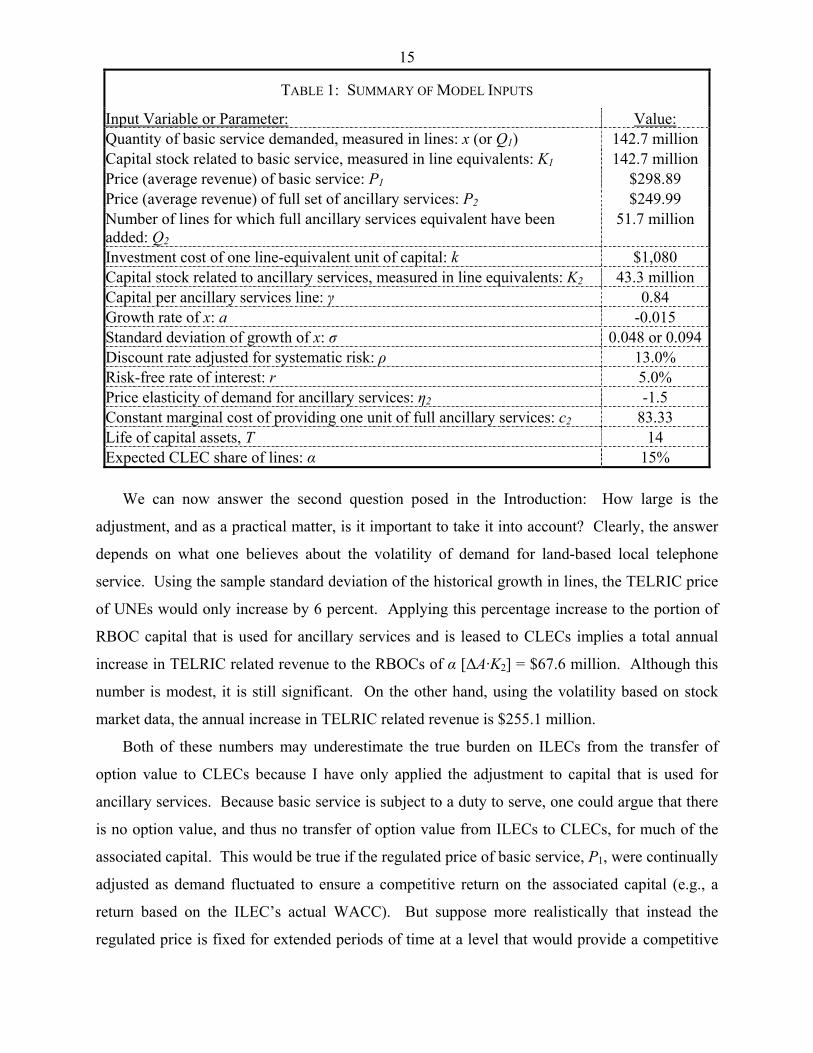
TABLE 1: SUMMARY OF MODEL INPUTS

Input Variable or Parameter: Value:Quantity of basic service demanded, measured in lines: x (or Q1) 142.7 million Capital stock related to basic service, measured in line equivalents: K1 142.7 million Price (average revenue) of basic service: P1 $298.89 Price (average revenue) of full set of ancillary services: P2 $249.99 Number of lines for which full ancillary services equivalent have been added: Q2

51.7 million

Investment cost of one line-equivalent unit of capital: k $1,080 Capital stock related to ancillary services, measured in line equivalents: K2 43.3 million Capital per ancillary services line: γ 0.84 Growth rate of x: a -0.015 Standard deviation of growth of x: σ 0.048 or 0.094Discount rate adjusted for systematic risk: ρ 13.0% Risk-free rate of interest: r 5.0% Price elasticity of demand for ancillary services: η2 -1.5 Constant marginal cost of providing one unit of full ancillary services: c2 83.33 Life of capital assets, T 14 Expected CLEC share of lines: α 15%

We can now answer the second question posed in the Introduction: How large is the

adjustment, and as a practical matter, is it important to take it into account? Clearly, the answer

depends on what one believes about the volatility of demand for land-based local telephone

service. Using the sample standard deviation of the historical growth in lines, the TELRIC price

of UNEs would only increase by 6 percent. Applying this percentage increase to the portion of

RBOC capital that is used for ancillary services and is leased to CLECs implies a total annual

increase in TELRIC related revenue to the RBOCs of α [∆A·K2] = $67.6 million. Although this

number is modest, it is still significant. On the other hand, using the volatility based on stock

market data, the annual increase in TELRIC related revenue is $255.1 million.

Both of these numbers may underestimate the true burden on ILECs from the transfer of

option value to CLECs because I have only applied the adjustment to capital that is used for

ancillary services. Because basic service is subject to a duty to serve, one could argue that there

is no option value, and thus no transfer of option value from ILECs to CLECs, for much of the

associated capital. This would be true if the regulated price of basic service, P1, were continually

adjusted as demand fluctuated to ensure a competitive return on the associated capital (e.g., a

return based on the ILEC’s actual WACC). But suppose more realistically that instead the

regulated price is fixed for extended periods of time at a level that would provide a competitive

16

return on the ILEC’s capital in the absence of CLEC entry. In other words, the price would be

set at a sufficiently high level that during times of high demand and full capacity utilization, the

ILEC would earn a higher-than-competitive return to compensate for lower returns during

periods of low demand. In that situation, CLECs would have an incentive to enter and use the

ILEC’s capital to provide basic service when demand is high, but not enter (or exit) when

demand is low. The CLEC would then earn a higher-than-competitive return on average, while

the ILEC earned a lower-than-competitive return. Given the duty to serve, the impact of this

forced transfer of profits on ILEC investment and consumer welfare is unclear. However, to

eliminate the transfer, regulators would have to expand the capital stock to which the TELRIC

adjustment is applied to include capital used to provide basic service.

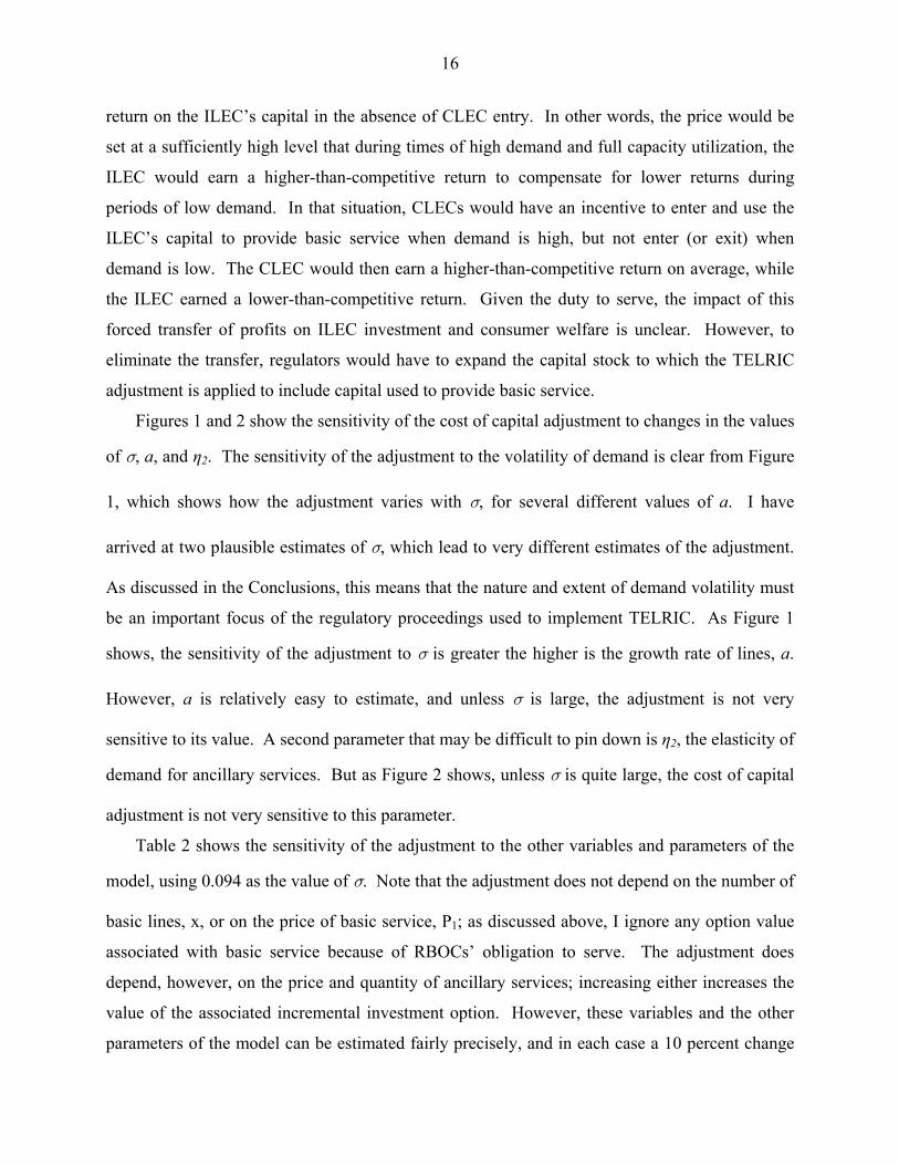
Figures 1 and 2 show the sensitivity of the cost of capital adjustment to changes in the values

of σ, a, and η2. The sensitivity of the adjustment to the volatility of demand is clear from Figure

1, which shows how the adjustment varies with σ, for several different values of a. I have

arrived at two plausible estimates of σ, which lead to very different estimates of the adjustment.

As discussed in the Conclusions, this means that the nature and extent of demand volatility must

be an important focus of the regulatory proceedings used to implement TELRIC. As Figure 1

shows, the sensitivity of the adjustment to σ is greater the higher is the growth rate of lines, a.

However, a is relatively easy to estimate, and unless σ is large, the adjustment is not very

sensitive to its value. A second parameter that may be difficult to pin down is η2, the elasticity of

demand for ancillary services. But as Figure 2 shows, unless σ is quite large, the cost of capital

adjustment is not very sensitive to this parameter.

Table 2 shows the sensitivity of the adjustment to the other variables and parameters of the

model, using 0.094 as the value of σ. Note that the adjustment does not depend on the number of

basic lines, x, or on the price of basic service, P1; as discussed above, I ignore any option value

associated with basic service because of RBOCs’ obligation to serve. The adjustment does

depend, however, on the price and quantity of ancillary services; increasing either increases the

value of the associated incremental investment option. However, these variables and the other

parameters of the model can be estimated fairly precisely, and in each case a 10 percent change

17

in the estimate leads to a fairly small change in the calculated adjustment. Thus, in terms of

actually applying the model, the greatest challenge remains estimating the volatility σ.

Note: Elasticities calculated holding all other variables constant except as noted: c1 varies with P1 so that the zero economic profits condition holds. Elasticities with respect to Q2 and K2 are calculated adjusting γ such that γ = K2 / Q2. The elasticity with respect to γ (holding Q2 fixed) is equal to the elasticity with respect to K2. Elasticity with respect to ρ(r) is calculated assuming r is changing such that r = .05 +/- .1 * ρ. Elasticities of P2’ and η2’ are calculated by adjusting c2 such that c2 = [(P2 * η2) + P2]/ η2.

TABLE 2: SENSITIVITY OF COST OF CAPITAL PREMIUM TO TEN PERCENT CHANGES IN THE INPUT VARIABLES (FOR σ = 0.094)

Input Variable Implied ElasticityQuantity of basic service demanded, measured in lines: x (or Q1) 0.0 Price (average revenue) of basic service: P1 0.0 Price (average revenue) of full set of ancillary services: P2 0.8 Number of lines for which full ancillary services equivalent have been added: Q2 1.0 Investment cost of one line-equivalent unit of capital: k -0.8 Capital stock related to ancillary services, measured in line equivalents: K2 -0.9 Growth rate of x: a -0.1 Discount rate adjusted for systematic risk: ρ -1.3 Price elasticity of demand for ancillary services: η2 -0.4 Constant marginal cost of providing one unit of full ancillary services: c2 0.1 Life of capital assets, T -0.3 Expected CLEC share of lines: α 0.0 Standard deviation of growth of x: σ 2.0 Other elasticities: ρ(r) -0.2 P2’ 0.9 η2’ 0.3

18

Figure 1: Sensitivity of Cost of Capital Adjustment to Volatility

0.000

0.010

0.020

0.030

0.040

0.050

0.060

0.070

0.080

0.03 0.035 0.04 0.045 0.05 0.055 0.06 0.065 0.07 0.075 0.08 0.085 0.09 0.095 0.1

Volatility, σ

Prem

ium

a = -0.030

a = -0.015

a = 0.015

a = 0

Figure 2: Sensitivity of Cost of Capital Adjustment to Elasticity of Demand

0.000

0.010

0.020

0.030

0.040

0.050

0.060

-0.9 -1.1 -1.3 -1.5 -1.7 -1.9 -2.1 -2.3 -2.5

Price Elasticity for Ancillary Services, η2

Prem

ium

Note: The cost of providing vertical services, c2, is adjusted, via the monopoly markup formula, as η 2 is changed.

σx = 0.094

σx = 0.048

19

4. Conclusions.

For better or for worse, mandatory unbundling and facilities sharing has become a central

part of the regulatory framework that governs telecommunications, and has also been used in

other industries. To apply this framework, however, it is essential to correctly determine the

lease rates that entrants should pay incumbents for the use of the incumbents’ facilities. In the

case of telecommunications, the TELRIC formula by which these lease rates are set

undercompensates incumbents because it ignores the irreversibility of their capital investments

and the corresponding transfer of option value to entrants. This, in turn, creates a disincentive

for ongoing investment by incumbents.

Although this problem has been pointed out by others, there has been no consensus as to its

importance, or how TELRIC or related pricing formulas can be altered to correct the problem.

The model developed in this paper provides a fairly simple method for correcting TELRIC – an

adjustment to the cost of capital used as an input to the TELRIC formula. As I have shown, that

adjustment can be calculated from a set of basic market variables. Using aggregate U.S. data for

the four RBOCs, I have shown that for the U.S. as a whole, the adjustment is significant, and the

current TELRIC formula substantially undercompensates incumbents. The actual size of the

adjustment, however, depends critically on the volatility of demand growth.

We have seen that estimating demand volatility is not straightforward, and one can arrive at

alternative estimates that are plausible but sufficiently different to lead to quite different cost of

capital adjustments. This is typical in models of irreversible investment and the valuation of

“real options.” One might think that this is a weakness of the approach proposed in this paper,

but it is not. On the contrary, it can re-focus the deliberations of regulatory agencies on what

really matters, rather than inputs that are of marginal importance in setting prices. In state

proceedings, for example, inordinate time and resources have been spent on the question of

whether an ILEC’s historic average cost of capital is 12.9 versus 13.1 percent. We have seen

that the correct cost of capital input for TELRIC should be significantly larger than either of

these numbers; at issue is whether it should be larger by about 1 percentage point or 4 to 5

percentage points. The answer depends on the extent of demand volatility looking forward, and

that should be the focus of regulatory deliberations.

The cost-of-capital adjustments that I have estimated are based on a calibration using

aggregate and average numbers for the U.S., and a calibration for a particular state or region

20

could differ considerably. Capital stocks, CLEC penetration, average line growth, and volatility

all differ considerably across different regions of the country, and such differences are one

reason that TELRIC rates currently differ so much across regions. However, all of the inputs

needed to apply the method proposed here are already available, or could easily be estimated, on

a regional basis. Thus the implementation of this method by state regulatory agencies should be

fairly straightforward.

Finally, it is important to reiterate that there is a question as to whether the adjustment to

TELRIC should be applied only to capital used for ancillary services, or also to some or all of the

capital used to provide basic service. Although basic service is subject to a duty to serve

(suggesting that there is no transfer of option value from ILECs to CLECs), regulated prices of

basic service are not continually adjusted to ensure a competitive return on the associated capital.

This creates an opportunity for CLECs to earn supracompetitive profits by entering or exiting in

response to changes in demand, which in turn generates a transfer of option value similar to that

for ancillary services. To eliminate the transfer, the capital stock to which the TELRIC

adjustment is applied would have to include some or all of the basic services capital.

21

APPENDIX A – DATA AND MODEL CALIBRATION

This appendix provides additional details on the estimation of the various inputs to the

model, including data sources.

Prices and Quantities of Ancillary Services. Table A-1 reports the monthly residential

prices (for selected areas) of both a comprehensive local service bundle and a basic local service

offering without any ancillary services from each the four RBOCs in 2002.21 Subtracting the

price of basic service from the bundled price yields estimates of monthly prices for a

comprehensive bundle of each provider’s ancillary services.22

TABLE A-1: RBOC ANNUALIZED AVERAGE PRICE FOR A FULL BUNDLE OF

RESIDENTIAL ANCILLARY SERVICES

Company Total Bundle Basic PriceAncillary

Services PriceVerizon $38.95 $16.34 $22.61 SBC $38.90 $16.82 $22.08 BellSouth $34.00 $15.40 $18.60 Qwest $34.99 $14.95 $20.04 Average $36.71 $15.88 $20.83 Annualized Average Price (P2) $440.52 $190.53 $249.99

Note: Ancillary Services Price calculated as Total Bundle Price minus Basic Service Price. Prices obtained from Banc of America Securities, Wireline Service Pricing, Sept. 22, 2003, p. 10. Prices do not include taxes and fees.

This estimate is for residential prices. An informal phone survey of the four RBOCs provided

information on how their prices of ancillary services for business lines compared to their prices

of these services for residential lines. The business prices varied considerably, but on average

they were similar to the residential ancillary services prices (see Table A-2 below). I use the

more accurately measured annual ancillary services price of $249.99, shown in Table A-1.

We also need the quantity, Q2, of the full ancillary services equivalent number of lines for

which those services were added. For example, a customer who purchases the full range of these

services has one unit of Q2, but a customer who purchases only one such service, say voicemail,

has a fraction of one unit of Q2. Thus Q2 is estimated by dividing the total revenues that RBOCs

receive from offering ancillary services, R2, by the average price of a full set of these services.

21 Banc of America Securities, Wireline Service Pricing, September 22, 2003, p. 10. 22 The ancillary service bundles include a combination of features, such as voicemail, caller ID, 3-way calling, call forwarding, call blocking and speed dial, but do not include long distance service.

22

For 2003, revenue was $12.9 billion,23 so dividing by P2 = $249.99 gives Q2 = 51.7 million.

TABLE A-2: RBOC ANNUALIZED AVERAGE PRICE FOR A FULL BUNDLE OF RESIDENTIAL AND BUSINESS ANCILLARY SERVICES

CompanyResidential Ancillary

Services PriceBusiness Ancillary

Services PriceAverage Ancillary

Services PriceVerizon $34.95 $15.00 $24.98 SBC $11.95 $34.16 $23.06 BellSouth $20.95 $12.90 $16.93 Qwest $20.00 $5.47 $12.74 Average $21.96 $16.88 $19.42 Annualized Average Price (P2) $263.55 $202.59 $233.07

Note: These prices were obtained through telephone inquiries with each company about the price of a single business / residential line with all available ancillary features. Pricing information is as of May 25, 2004, and was obtained for the following regions: BLS (Atlanta, GA), SBC (Houston, TX), Qwest (CO), VZ (New York City). These regions were selected to maintain consistency with Table A-1.

Investment Cost of One Line-Equivalent Unit of Capital. Table A-3 shows the

breakdown of RBOC operating revenues among the three activities and the implied breakdown

of the RBOCs’ $356.2 billion in Total Plant in Service (before amortizable assets). The implied

gross value of K1 = $154.1 billion, and the implied gross value of K2 = $46.7 billion. Dividing

$154.1 billion by x = 142.7 million lines gives k = $1,080.

TABLE A-3: CAPITAL STOCK CALCULATIONS, ALLOCATED BY REVENUE: 2003

Amount % of TotalTotal Basic Service Revenues $42,651,061 43.3% Total Ancillary Service Revenues $12,928,095 13.1% Total Other Revenues $42,980,515 43.6% Total RBOC Operating Revenues $98,559,671 100% Total TPIS (Before Amortizable Assets) $356,213,281 100% Basic Services Apportionment (Gross Value of K1) $154,148,996 43.3% Ancillary Services Apportionment (Gross Value of K2) $46,724,579 13.1% Other Services Apportionment $155,339,705 43.6%

Note: Capital data obtained from FCC Report 43-02, the ARMIS USOA Report, Table B.1.B, Balance Sheet Accounts (Plant Accounts). Amounts in thousands of dollars.

23 Data reflect “Other Basic Service Revenue” from FCC Report 43-03, the ARMIS Joint Cost Report, Table I, Regulated/Nonregulated Data.

23

Expected Growth Rate of x. I estimate the expected rate of growth of x (i.e., the drift rate a

in eqn. (2)) from the historical growth trend in RBOC lines. Table A-4 shows the weighted

average growth rates in the number of lines in each RBOC COSA for two time periods: 1996-

2003 and 1999-2003. Estimates of a range from -0.003 to -0.027. I use a = -0.015, which is the

average of the two growth rates.

TABLE A-4: ANNUAL GROWTH RATE OF RBOC LINES

1996-2003 1999-2003Growth Rate (Weighted By Number of Lines) -0.3% (+/-1.0%) -2.7% (+/-0.7%)

Note: Access lines data obtained from FCC Report 43-05, The ARMIS Service Quality Report, Table V., Service Quality Complaints. 1996 lines are accurate to the nearest 1000. All company states with missing or ‘zero’ observations are excluded from the dataset. Verizon NO-Contel/Illinois and Verizon SW-Contel-Texas are excluded from the dataset, because of large deviations in number of lines between 1999 and 2000. 95% confidence intervals are in parentheses.

These data on RBOC lines are also used to estimate σ, the standard deviation of the annual

rate of growth of x. For the period 1996-2003, the weighted estimate of the standard deviation is

0.048. However, as explained in Appendix B, σ can also be estimated from the standard

deviation of RBOC stock returns.

Stock Return Volatility and Volatility of x. To estimate the volatility of RBOCs’ assets,

σV, we calculate the 1-year and year-to-date averages of the 10-day historical unlevered

volatilities implied by the calls and puts on RBOC stocks. The results of these calculations are

shown in Table A-5 below. They imply an average value for σV of 0.148. Using eqn. (35) in

Appendix B, this in turn yields an estimate of σ equal to 0.094.

TABLE A-5: HISTORICAL IMPLIED UNLEVERED VOLATILITY OF RETURNS (AS OF OCTOBER 20, 2004)

Unlevered Volatility Verizon SBC BellSouthYear to Date Average 0.102 0.178 0.157 One Year Average 0.105 0.180 0.166

Source: Data from Bloomberg

24

APPENDIX B – ESTIMATING DEMAND VOLATILITY FROM STOCK MARKET DATA

This appendix shows how the parameter σ can be estimated indirectly from stock market

data. If we had stock market data for a “pure ILEC” and knew the debt-equity ratio for the

company, we could estimate the volatility of the equity, and from that determine the volatility of

the ILEC’s value. Of course, the stock market value for a company like Verizon will reflect

more than its ILEC activity. However, ILEC-related revenue is about two-thirds of Verizon’s

total revenue, and the fraction is similar for the other RBOCs. Thus I use RBOC stock price data

as a proxy for the value of a pure ILEC, denoted by V. As discussed in Appendix A, I use

unlevered stock returns for a set of three RBOCs to estimate the parameter σV in the equation:

/ V VdV V a dt dzσ= + (24)

We want to relate σV to the parameter σ in eqn. (2). To do this, we must determine the

relationship between the value of the ILEC, V, and the demand shift variable x. This is done by

breaking V down into two components: (1) the value to the ILEC of its current capital stock

K*(x); and (2) the value of the ILEC’s options to add more capital in the future, should demand

conditions warrant it. Write the value of the ILEC as V = Vc + Vf. One might ask why there is

any value to the ILEC’s options to add capital in the future, given the transfer of option value to

CLECs. The reason is that (at least to date) CLECs do not lease all ILEC capital. Typically,

only about 15 percent of ILEC capital is expected to be leased by CLECs, so an ILEC still has

option value that it retains. In what follows, I will assume that CLECs lease a fraction α of both

the ILEC’s basic lines and the ILEC’s capital devoted to ancillary services.

Value of ILEC’s Current Capital Stock. We begin with Vc, the value of the ILEC’s

current capital stock, which we will treat as fixed. The ILEC has three sources of revenue and

hence profit from this capital stock: (i) sales of basic service at the exogenously determined price

P1; (ii) sales of ancillary services at the endogenously determined price P2(Q2); and (iii) leasing

revenue from the CLEC for its use of part of the ILEC’s capital. To find Vc, we determine the

profit flow for each of these three components, and then determine the corresponding capitalized

value for the total profit flow. I assume throughout that the CLEC utilizes a fraction α of the

25

total capital stock.

(i) Revenue from Basic Service: The price of basic service is an exogenous (regulated)

input, and the quantity of sales for the ILEC is (1-α)x, so this component of profit is simply:

1 1(1 )( )P c x1π α= − − (25)

(ii) Revenue from Ancillary Services: For this segment, the price is given by .

The total quantity sold to this segment is in turn given by

2 2( )P b x Q= −

2 2 / ( ) /Q K K xγ γ= = − so the market

price can be written as:

2(1 )bP x b Kγγ γ+

= − (26)

We are calculating the value of the ILEC’s current capital stock, so the total capital stock K*(x),

which is given by eqn. (16), is fixed at its current value, which in turn is based on the current

value of x, i.e., x0. The ILEC utilizes a fraction (1-α) of the total capital, so its profit is

2 2(1 )( )P c Q2 2π α= − − (27)

Making the substitutions, this can be rewritten as:

2 '2 1 2A x A x Aπ '

3= − + − (28)

where A1, A2’, and A3

’ are given by:

1 2(1 ) (1 )bA α γ

γ− +

=

' 22 2

(1 ) (2 ) (1 )b cA Kα γ αγ γ

− + −= +

' 2 23 2

(1 ) (1 )b cA K Kα αγ γ− −

= +

(iii) TELRIC Revenue from CLEC: The last component of profit is the TELRIC revenue that

the ILEC receives from the CLEC. From eqn. (3), this is:

3(1 )

(1 ) 1

T

T kKρ ρπ αρ+

=+ −

(29)

Total Profit and Its Capitalized Value. The total flow of profit accruing to the ILEC from its

current stock of capital is 1 2 3π π π π= + + . Combining the three components above, we can

write the total profit as:

26

21 2A x A x Aπ 3= − + − (30)

where A1 is given above, and A2 and A3 are given by:

'2 2 1 1(1 )( )A A P cα= + − −

'3 3

(1 )(1 ) 1

T

TA A kKρ ραρ+

= −+ −

The value of this flow of profit is

00

( ; )T

cV E x e dρτπ τ −= ∫ τ (31)

Note that x follows the GBM of eqn. (2). Following the steps in Dixit and Pindyck (1994, page

82) to take the integral, the value is given by:24

22 ( 2 ) ( )

1 22

(1 ) (1 )( 2 ) ( )

T a T aT

cA x e A x e A DV

a a

ρ σ ρ3

ρ σ ρ

− − − − −− −= − + −

− − − ρ

2T

(32)

Value of ILEC’s Options to Add Capital in the Future. I turn now to Vf, the value of the

ILEC’s options to increase its capital stock in the future, should demand conditions warrant this.

For , the value of the ILEC’s option to invest in an incremental unit of capital is given

by eqn. (13), with B = B(K) given by eqn. (17). The value of the ILEC’s options to invest in

more capital is the sum of the value of its option to purchase one unit of capital beyond its

current capital stock K

*( )K K x≥

0, the value of its option to purchase another unit beyond that, and so on.

Because a fraction α of this option value is transferred to the CLEC, Vf is given by:

(33) *0 ( )

( ) (1 ) ( )fK x

V x B K x dKβα∞

= − ∫

Substituting eqn. (17) for B(K) and carrying out the integration, we have:

21 2(2 / )fV x bK c k Dβ βω γ γ ρ −= + + (34)

where

11

(1 ) ( 2) [ ( 1)]2 ( 2)

TD bb

ββα γω ρ

γ β βδβ −⎛ ⎞− +

= −⎜ ⎟− ⎝ ⎠

θ σ24 If x follows the GBM of eqn. (2), . 2( ( 1) / 2 2

0 00(1 ) /[ ( 1) / 2]

T T aE x e d x e aθ ρτ θ ρ θ θ θ στ ρ θ θ− − − − −= − − − −∫

27

Note that we must have β > 2 for Vf to remain finite, which in turn imposes an upper bound on σ.

(As σ becomes larger, β becomes smaller, approaching 1 in the limit.)

Total Value of ILEC. The total value of the ILEC, cV V Vf= + , is just the sum of the

components in eqns. (32) and (34). We can now relate dV/V to dx/x. From Ito’s Lemma,

2

22

d 1 dd d (dd 2 dV VV xx x

= + )x

However, we are only concerned with the stochastic components of dV and dx, so we can ignore

the second-order term. We therefore have ( )V dz x dzσ σ= Ω , where

( /( )( )

)x dV dxxV x

Ω = (35)

Note that dV/dx is given by:

2( 2 ) ( )

1 21 21 22

2 (1 ) (1 ) (2 / )( 2 ) ( )

T a T a

TdV A x e A e x bK c k Ddx a a

ρ σ ρ2β ββω γ γ ρ

ρ σ ρ

− − − − −− −− −

= − + + + +− − −

(36)

We measure σV, and evaluate Ω(x) at the calibrated (current) value of x, i.e., x0. Thus the

estimate of σ is obtained from 0ˆ ˆ / ( )V xσ σ= Ω .

28

REFERENCES Bourreau, Marc, and Pinar Dogan, “Unbundling the Local Loop,” European Economic Review,

Jan. 2005, 49, 173—199. Clarke, Richard N., Kevin A. Hassett, Zoya Ivanova, and Laurence Kotlikoff, “Assessing the

Economic Gains from Telecom Competition,” NBER Working Paper No. 10482, May 2004.

Crandall, Robert W., Allan T. Ingraham, and Hal J. Singer, “Do Unbundling Policies Discourage

CLEC Facilities-Based Investment?” B.E. Journals in Economic Analysis and Policy, Feb. 2004.

Dixit, Avinash K. and Robert S. Pindyck, Investment Under Uncertainty, Princeton University

Press, 1994.

Economides, Nicholas, Katja Seim, and V. Brian Viard, “Quantifying the Benefits of Entry into Local Phone Service,” unpublished, Feb. 2004.

Ford, George S., and Michael D. Pelcovits, “Unbundling and Facilities-Based Entry by CLECs: Two Empirical Tests,” July 2002, http://www.telepolicy.com/papers.htm.

Greenstein, Shane, and Michael Mazzeo, “Differentiation Strategy and Market Deregulation:

Local Telecommunication Entry in the Late 1990s,” NBER Working Paper No. 9761, June, 2003.

Hausman, Jerry A., “Valuing the Effect of Regulation on New Services in Telecommunications,” Brookings Papers on Economic Activity, Microeconomics 1997, pp. 1-54.

Hausman, Jerry A., “Regulated Costs and Prices in Telecommunications,” G. Madden, editor,

Emerging Telecommunications Networks, Edward Elgar Publishing, 2003. Hausman, Jerry A. and Stewart C. Myers, “Regulating the United States Railroads: The Effects

of Sunk Costs and Asymmetric Risk,” Journal of Regulatory Economics, 2002, Vol. 22, pp. 287-310.

Hausman, Jerry A., and J. Gregory Sidak, “Did Mandatory Unbundling Achieve Its Purpose? Empirical Evidence from Five Countries,” Journal of Competitive Law and Economics, forthcoming, 2005.

Hazlett, Thomas W., Arthur M. Havenner, and Coleman Bazelon, Declaration Submitted to the Federal Communications Commission by Verizon Communications, WC Docket No. 03-157 September 2, 2003.

Jorde, Thomas M., J. Gregory Sidak, and David J. Teece, “Innovation, Investment, and Unbundling,” Yale Journal of Regulation, Winter 2000, Vol. 17.

29

Kahn, Alfred E. Lessons from Deregulation, AEI-Brookings Joint Center for Regulatory

Studies, Washington, D.C., 2004. Knittel, Christopher R., “Regulatory Restructuring and Incumbent Price Dynamics: The Case of

U.S. Local Telephone Markets,” Review of Economics and Statistics, May 2004, Vol. 86, pp. 614-625.

Kotakorpi, Kaisa, “Access Price Regulation, Investment and Entry in Telecommunications,”

Unpublished, Department of Economics, University of Tampere, Finland, June 2004. Phoenix Center Policy Bulletin No. 5, “Competition and Bell Company Investment in

Telecommunications Plant: The Effects of UNE-P,” July 9, 2003 (updated Sept. 17, 2003), http://www.phoenix-center.org/pbulletin.html.

Pindyck, Robert S. “Irreversible Investment, Capacity Choice, and the Value of the Firm,”

American Economic Review, December 1988, Vol. 79, pp. 969-985. Pindyck, Robert S. “Mandatory Unbundling and Irreversible Investment in Telecom Networks”

NBER Working Paper No. 10287, January 2004. Salinger, Michael A., “Regulating Prices to Equal Forward-Looking Costs: Cost-Based Prices or

Price-Based Costs?” Journal of Regulatory Economics, 1998, Vol. 14, pp. 149-163.

Tardiff, Timothy J., “The Forecasting Implications of Telecommunications Cost Models,” James Alleman and Eli Noam, editors, The New Investment Theory of Real Options and Its Implication For Telecommunications Economics, Kluwer Academic Publishers, 1999, pp. 181-190.

Vander Weide, James H., Testimony on behalf of Verizon Virginia Inc., Docket Nos. 00-218, 00-249, 00-251, April 15, 2003, p. 16 and Attachment 2.

Willig, Robert D., William H. Lehr, John P. Bigelow, and Stephen B. Levinson, “Stimulating

Investment and the Telecommunications Act of 1996,” unpublished, October 2002.