nber working paper series energy, … should have reduced the price that they were willing to pay...
TRANSCRIPT

NBER WORKING PAPER SERIES
ENERGY, OBSOLESCENCE,AND THE PRODUCTIVITY SLOWDOWN
Charles R. Hulten
James W. Robertson
Frank C. Wykoff
Working Paper No. 2404
NATIONAL BUREAU OF ECONOMIC RESEARCH1050 Massachusetts Avenue
Cambridge, MA 02138October 1987
We gratefully acknowledge the financial support by the Bureau of Labor Statistics,U.S. Department of Labor. The findings and opinions presented in this paper arestrictly those of the authors and should not be attributed to BLS. We wish tothank Jerome Mark and William Waldorf of the Bureau of Labor Statistics, M. Wolfsonof the Machinery Dealers National Association, Lloyd Sommers, and Victor Wykoffof Caterpillar Tractor Co. for their support and encouragement, and Ernst Berndt,Michael Harper, Dale Jorgenson, and Reza Ragozar for their comments and help.The research reported here is part of the NBERs research program in Productivity.Any opinions expressed are those of the authors and not those of the National
Bureau of Economic Research.
NBER Working Paper #2404October 1987
Energy, Obsolescence, and the Productivity Slowdown
ABSTRACT
The growth rate of output per worker in the U.S; declined sharplyduring the 1970's. A leading explanation of this phenomenon holds that
the dramatic rise in energy prices during the 1970's caused a significantportion of the U.S. capital stock to become obsolete. This led to adecline in effective capital input which, in turn, caused a reduction inthe reduction in the growth rate of output per worker.
This paper examines a key prediction of this hypothesis. If there isa significant link between energy and capital obsolescence, it should berevealed in the market price of used capital: if rising energy costs didin fact render older, energy-inefficient capital obsolete, prospectivebuyers should have reduced the price that they were willing to pay forthat capital. An examination of the market for used capital before andafter the energy price shocks should thus reveal the presence andmagnitude of the obsolescence effect.
We have carried out this examination for four types of used machinetools and five types of construction equipment. We did not find ageneral reduction in the price of used equipment after the energy priceshocks. Tndeed, the price of used construction equipment - the more
energy intensive of our two types of capital - tended to increase after
1973. We thus conclude that our data do not support the obsolescenceexplanation of the productivity of slowdown.
Charles R. Hulten James W, Robertson Frank C. Wykoff
Chairman Maxwell Stamp Associates Department of Economics
Department of Economics London Pomona College
University of Maryland ENGLAND Claremont, CA 91711
College Park, MD 20742

Energy, Obsolesence, and the Productivity Slowdown
Output per worker in the U.S. business sector grew at an average annual
rate of 3.0% from 1948 to 1973. From 1973 to 1984, however, this annual rate
plunged to 1.1%. This is the widely publicized "productivity slowdown" that
has attracted so much attention from economic researchers.1
Some analysts see the slowdown as a consequence of the changing structure
of the U.S. economy - the increased importance of international trade, the
shift in economic activity towards the seivice sector, and the changing
demography of the labor force; others see the problem resulting from policy
inflicted wounds such as increased tax burdens on income from capital and
increased regulatory requirements; still others see the problem as due to
macroeconomic trends in inflation and recession. Some even hold the view that
the slowdown is an artifact of the data and really did not occur at all.2
A prime suspect, however, is the rapid and unexpected rise in energy
prices imposed by the OPEC cartel in 1973 and again in 1979. While there is
still a debate over when the productivity slowdown started, few doubt that the
sharpest decline occurred after 1973. The coincidence of this decline in most
industrialized countries with the energy crisis is an obvious clue, and many
analysts have suggested mechanisms through which higher energy prices cause
economic growth to slow.
In this paper we examine one of the leading energy-related hypotheses.
This hypothesis, advanced by Martin N. Baily (1981), holds that the rise in
energy prices accelerated the rate of obsolescence of the U.S. stock of
physical capital. Since conventional measures of the capital stock do not
capture changes in the rate of obsolescence, conventional analyses of growth
1
fail to identify this effect. Instead, they suppress it into a time trend or
residual estimate of productivity change. Baily shows that this
energy-induced obsolescence effect may have been large enough to account for
most of the productivity slowdown.
If correct, the obsolescence hypothesis offers a sufficient explanation
of the productivity slowdown. Baily's evidence is, however, based on the
correlation between the rise in energy prices and the decline in Tobin's
average q, and is subject to the criticism that the q ratio could have fallen
during the 1970's for reasons unrelated to the energy crisis (e.g. the rise in
effective income tax rates).3 A more direct test is needed to establish the
extent to which the energy price increases induced obsolescence in the stock
of capital.
The model of this paper provides such a test. If there is a significant
link between energy and obsolescence, it should be revealed in the price of
old capital: if rising energy costs did in fact render older,
energy-inefficient capital obsolete, prospective buyers should have reduced
the price that they were willing to pay for that capital (a decline in asset
value is, indeed, the definition of obsolescence).4 An examination of the
market price of used capital before and after the energy price shocks should
thus reveal the sign and the magnitude of the Baily effect.
We have carried out this examination for four types of used machine tools
and five types of construction equipment. Our principal conclusion is that
data for these assets do not support the obsolescence hypothesis. There is
no systematic downward shift in used asset prices after 1973, and, for
construction equipment, the shifts tend to be upward, not downward.5
The paper is organized as follows: In sections II and III we review the
2
recent literature on the role of energy in the productivity slowdown. In the
subsequent two sections we set out our model of used asset prices and relate
it to the obsolescence hypothesis. We then describe our data and present the
empirical findings in sections VI and VII.
II. Energy and Economic Growth
Energy can be directly related to economic growth via a production
function in which gross output, Q, is assumed to depend on the quantities of
capital, K, labor, L, energy, E, and material inputs, H:6
(1) Q = A F(K,L,E,H).
In the production function (1), all variables are implicit functions of time
and the variable A is included separately to allow for Hicks-neutral shifts in
the function over time, i.e., to allow for changes in Q not captured by
changes in the input quantities. The term A is thus a surrogate for technical
change, but also includes the effects of such factors as managerial efficiency
and worker effort.
The fundamental equation of growth analysis can be derived from the
production function under the assumption that each input is paid the value of
its marginal product. Logarithmic differentiation of F yields:7
(2) Q=SKK+SLL+SEE+SMH+A.
Hats over variables indicate rates of growth, and S's represent the shares of
total cost allocated in each input; 5L' for example, represents labor's share
3
A
of total costs; the variable A represents the rate at which the technology
shifts over time (and is called the rate of change of total factorA
productivity). All variables in (2) except A can be measured directly orA
imputed, so A can be measured as a residual.
If one assumes constant returns to scale, then the cost shares sum to one
and (2) can be written as
(3) Q-L = SK(KL) + SE(EL) + SE(ML) + A.
The left hand side of equation (3) is the growth rate of output per labor-hour
- "labor productivity." Equation (3) states that labor productivity equals
the sum of the growth rate of the capital-labor ratio, weighted by capital's
share of total cost, the growth rates of energy and materials per labor-hour,
weighted by their cost shares, and the growth rate of total factor
productivity.
Equation (3) provides a framework for analyzing the slowdown in laborA A
productivity. Any change in Q-L after 1973 must be associated with changes in
the variables on the right hand side of (3). In particular, the impact of the
energy costs on Q/L can be linked directly to changes in the energy intensity
of production, E/L. This link suggests the following explanation for the
productivity slowdown: the rise in the price of energy relative to other
input prices caused the demand for energy to fall and this reduced the growthA A A A
rate of E-L, which caused Q-L to slow.
This explanation for the slowdown was among the first considered.8
However, the problem with this explanation is that energy's cost share (SE)is
very small, about 2% for U.S. manufacturing, so that even large changes in E-L
4
A Awill have a small impact on Q-L. An even more important problem is that, for
U.S. manufacturing industries, the decline in E after 1973 was largely offset
by a concomitant decline in L. Thus, according to data from the Bureau ofA A
Labor Statistics, covering the period 1948-1981, almost no change in E-L
occurred after 1973. This data - shown in Table 1 - leads to the conclusion,
expressed in a similar study by Berndt (1980) that "energy price or quantity
variations since 1973 do not appear to have played a significant direct or
indirect role in the slowdown of labor productivity in U.S. manufacturing"
(p.72).
Another possible link between energy and economic growth was advanced by
Hudson and Jorgenson (1978) and Berndt and Wood (1979). If energy and capital
are complements in production, an increase in the price of energy should
reduce the demand for capital and trigger a substitution of other inputs for
capital. The impact of higher energy costs would then appear as a reduction
in the growth rate K/L, as well as in the E/L term of (3). Unfortunately, the
data of Table 1 do not support this hypothesis either: the decline in E/L is
small and explains only 5% of the decline in the growth of Q/L, while the
growth rate of the traditionally measured capital-labor ratio actually
increased after 1973.
According to the estimates of Table 1, the slowdown in labor productivity
is entirely related to a decline in the growth rate of total factor
productivity. This would appear to exonerate the energy crisis as the primary
cause of the productivity slowdown, and to shift attention to the residual
variable A that some call "a measure of our ignorance." This conclusion,
however, presumes that the price of energy and the growth rate of total factor
productivity are not linked. In fact, two such links have been established.
5

Table 1.
The Productivity Slowdown in U.S. Manufacturing
1949-81 1949-73 1973-81
Average Annual WeightedGrowth Rates
(percentage points)
output/labor 2.20 2.57 1.07
capital/labor* 0.52 0.47 0.67
energy/labor* 0.05 0.07 -0.01
material/labor* 0.40 0.41 0.38
service/labor* 0.29 0.27 0.34TFP 0.92 1.34 -0.31
Unweighted Average AnnualGrowth Rates of Inputs
(percentage points)
capital 3.92 3.86 4.11labor 1.05 1.49 -0.25
energy 3.67 5.05 -0.43materials 2.70 3.18 1.28services 4.95 5.44 3.49
Cost shares
(percent)
capital .18 .19 .14labor .50 .50 .50
energy .02 .02 .05material .23 .23 .23services .07 .06 .08
1.00 1.00 1.00
*weighted by cost sharesSource: Bureau of Labor Statistics (1985)
First, Jorgenson and Fraumeni (1981) and Jorgenson (1984) have argued that
total factor productivity depends on the price of energy through a bias in
6
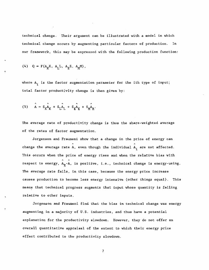
technical change. Their argument can be illustrated with a model in which
technical change occurs by augmenting particular factors of production. In
our framework, this may be expressed with the following production function:
(4) Q = F(AKK ALL. AEE AMN).
where A. is the factor augmentation parameter for the ith type of input;
total factor productivity change is then given by:
(5) ASKAg+SLAL+SEAE+SMAM.
The average rate of productivity change is thus the share-weighted average
of the rates of factor augmentation.
Jorgenson and Fraumeni show that a change in the price of energy can
change the average rate A, even though the individual A are not affected.
This occurs when the price of energy rises and when the relative bias withA A
respect to energy, AEA is positive, i.e., technical change is energy-using.
The average rate falls, in this case, because the energy price increase
causes production to become less energy intensive (other things equal). This
means that technical progress augments that input whose quantity is falling
relative to other inputs.
Jorgenson and Fraumeni find that the bias in technical change was energy
augmenting in a majority of U.S. industries, and thus have a potential
explanation for the productivity slowdown. However, they do not offer an
overall quantitative appraisal of the extent to which their energy price
effect contributed to the productivity slowdown.
7
III. The Baily Hypothesis
The second link between energy costs and total factor productivity
was developed by Martin N. Baily (1981). Baily noted that conventional
measures of capital stock do not allow for changes in the rates of utilization
or variations in the rates of depreciation of capital. Instead, the capital
stocks are typically measured using a perpetual inventory method - that is, by
cumulating investment during year t and subtracting the depreciation and
retirement of the existing stock. Depreciation and retirement are assumed to
be stationary processes which do not change with economic events.
According to Baily, this method of estimating capital is inadequate for
measuring the contribution of capital to the growth of output, since the sharp
rise in energy costs may have caused firms to utilize their old
energy-inefficient capital less intensively and to retire it earlier. A
trucking company, for example, may have had the incentive to operate its
relatively energy-efficient trucks more frequently, and reserve its less
efficient vehicles for peak load capacity. In this case, the rise in energy
costs causes the trucking firm to some use of its capital less intensively.
Yet, perpetual inventory measures of capital, by their very nature, cannot
capture this effect.
An important conclusion follows from this line of analysis: If
utilization effects are present, they will be suppressed into the residual
estimate of total factor productivity and thus misstate the impact of energy
prices on capital. To illustrate this mismeasurernent problem formally, let
*K denote the true growth rate of capital input (i.e. the rate adjusted for
utilization) and A* the true rate of total productivity growth; equation (3)
8

then becomes
A A A* A A A A A
(6) Q-L = SK(K -L) + SE(E -L) + SM(M -L) + A
Comparing (3) and (6), we find that
A A* A* A(7) A = A +
SK(K -K).
A A
If K overstates K because utilization is ignored, then A will be biasedA* A
downward by an amount equal to the change in utilization (K -K) multiplied by
capital's share in total cost. It follows immediately that the sharp decline
in the conventionally measured growth rate of total factor productivity after
1973, evident in the estimates of Table I (which are based on perpetualA
inventory calculations of K), may have been caused instead by an
energy-induced decline in the rate of utilization of old capital.9
Any test of the Baily hypothesis must deal with the difficult problem of
measuring the unobserved variable K*. Baily provides an ingenious solution
to this problem: he assumes a "putty-putty" Cobb-Douglas technology in which
input substitution can occur both yost and ante; he then derives a
production function in which output depends on the value of the capital stock
rather than on the quantity of capital. In our framework, this implies that
the production function has the form:
* * *(8) Q = F(K ,L,E,M,A ) F(VK,L,E,M,A ),
*with the value of the stock (VK) substituted for the quantity of capital K
9

In this model, variations in the value of the capital stock act as a surrogate
for variations in the utilization of this stock, given K.
The VK in (8) nominally refers to the present value of the income
associated with the stock of capital. VK is therefore equal to the amount
that rational investors would be willing to pay for the capital, and should
thus be equal to the financial value of the firm (less "goodwill"). A
*financial measure of VK could thus be used as a surrogate for K
Baily, however, uses a slightly different approach based on Tobin's q
theory of investment decision. Tobin's average q as is defined as
(9) q = VK/P1K,
(where P1 is the price of a new unit of capital stock, and P1K is the
replacement cost of the capital stock). In view of (9) we can write VK as
qP1K and substitute the result into the production function. Since K is
measured in physical units and P1 is the price of new investment goods, an
obsolescence induced decline in VK is reflected in q.
According to Summers (1981), Tobin's q fell during the 1970's (from
1.029 in 1973 to 0.747 in 1977), and Baily concludes that the movement in q is
more than sufficient to explain the productivity slowdown. The obsolescence
hypothesis thus provides a complete explanation of the productivity puzzle.
There are, however, at least two difficulties with this explanation.
First, the decline in Tobin's q could be due to any number of factors, not
just energy price shocks. Summers, for example, writing in the same volume as
Baily, attributes the decline in q to perverse tax policy. Indeed, Baily
himself is careful to note that the decline in effective capital stock may
10
have been caused by structural changes in the U.S. economy due to such factors
as increased foreign trade. The use of Tobin's q to explain the total factor
productivity residual may simply substitute one "measure of ignorance" for
another.
The second problem with using q theory arises because changes in the
value of the capital stock due to obsolescence do not necessarily imply
changes in the effectiveness of capital used in production. In Solow's
vintage model, for example, the introduction of superior new capital reduces
the net income accruing to old capital, but this capital continues to be
operated so long as the net income of the vintage is positive. And, as we
shall see below, it is even possible that older capital is operated more
intensively for a period of time after the energy price shock renders old
capital obsolete. This can occur if there is substantial uncertainty about
the nature and speed of introduction of new energy saving technology.
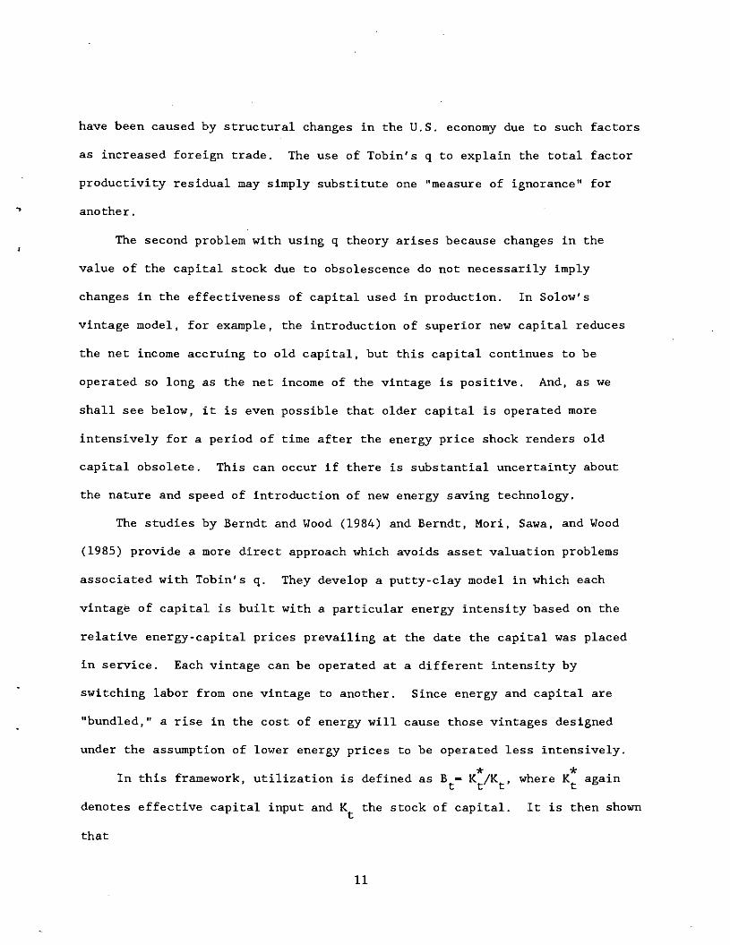
The studies by Berndt and Wood (1984) and Berndt, Mori, Sawa, and Wood
(1985) provide a more direct approach which avoids asset valuation problems
associated with Tobin's q. They develop a putty-clay model in which each
vintage of capital is built with a particular energy intensity based on the
relative energy-capital prices prevailing at the date the capital was placed
in service. Each vintage can be operated at a different intensity by
switching labor from one vintage to another. Since energy and capital are
"bundled," a rise in the cost of energy will cause those vintages designed
under the assumption of lower energy prices to be operated less intensively.
In this framework, utilization is defined as Bt= K7K. where K again
denotes effective capital input and the stock of capital. It is then shown
that
11

3 in B
(10) = - aa in
EK,t
where is the expected relative price of capital services and energy and
a is the ex ante elasticity of substitution between capital and energy. From
(7), it is evident that changes in introduce biases in the measurement of
total factor productivity. Indeed, (7) can be rewritten as
A A* A
(7') A = A + SKBt.
This expression, in conjunction with (10), ties the inismeasureinent of total
factor productivity growth directly to changes in the expected price of
energy.
Berndt and Wood (1985) report an average reduction in B of 29% between
1973 and 1974, and a net change of 5% between 1973 and 1978. The second
energy price shock reduced B by 7% between 1979 and 1980, and by 3% between
1979 and 1981. This pattern suggests that the Berndt-Wood correction is
primarily cyclical and that the secular change in over the 1970's was much
more modest. Indeed, the average annual growth rate of lit. t. was 2.1%
over the period 1973-81. Since capital's share of income was .14 for this
period (according to Table 1), (7') implies a correction of 0.3% per year in
A
A. Since measured total factor productivity grew at an average annual rate of
1.34% over the period 1949-73, and then declined to -0.31% over the period
1973-81, the Berndt-Wood correction is not large enough to explain the declineA
in A as measured error.
This finding is repeated in Berndt et al. (1985), who relate (10) to the
12

sources of growth model (2), using a somewhat different rationale for (10).
They find that, even when large values of a are assumed, the implied
utilization correction explains almost none of the productivity slowdown in
U.S. manufacturing. In sum, the results of Berndt et al. do not appear to
support the hypothesis that the energy crises was the primary cause of the
productivity slowdown.
IV. The Vintage Price Approach
We adopt in this study a variant of Baily's willingness-to-pay approach
that avoids Tobin's q theory. Instead of inferring the value of capital stock
(VK) from financial data which values the entire firm, we estimate capital
value directly from market data on used equipment prices. This is possible
because, at any time t, the aggregate value of the capital stock is the sum
of the values of the separate vintages:
Tmax
(11) VK= V P KI,ss
s=0
This equation indicates that, in principle, VK could be measured by valuing
the separate components of physical capital assets.
We assume that the P1 in (11) are equal to the amount an investor would
be willing to pay for a piece of capital. This, in turn, is assumed to be
equal to the present value of the expected net income stream generated by the
asset. For an s-year old asset, this present value is given by:
13

T
1'K,s+t
(12) =t÷l
t=o (in)
where T is the optimal retirement age of an s-year old asset, r is the
constant expected discount rate, and K,s+t is the expected net income flow
accruing to the asset of age s+t years in the future. Under constant returns
to scale,
Q L E M5 5 5 5
(13) 1'K= - - -
K K K5 5 $ 5
since the value of the output produced by a unit of capital just equals the
cost of all the inputs. In a putty-clay model, the quantity ratios are fixed
and a rise in P , ceteris yaribus, will cause P to fall. The lower netE K,s
yield to energy-using capital is reflected in and is lrcapitalizedrt in
price of used capital via (12). Furthermore, the percentage decline in price
will tend to increase with age and the optimal time to retirement will be
shortened. These capitalization effects occur without variation in
utilization. They will be reinforced if assets of vintage-s are utilized less
intensively, as Baily and Berndt et al. postulate.
The geometric interpretation of this model is given in Figure 1. The
curve PA is the locus of prices plotted against age, s, for a given year
t. The curve AA is depicted with a negative slope, reflecting the fact that
the value P15 falls with increasing age because: (1) the date of retirement
14

is drawing closer (i.e. because T is smaller); and (2) older assets may
generate less income because of increased maintenance expenses or decreased
productivity (i.e. because is smaller), While we have drawn this
"age-price" profile as convex, following the findings of Hulten and Wykoff
(l98la, l98lb), the profile could, in principle, be linear, concave, or
irregular.
The capitalization effects discussed above are illustrated in Figure 1 by
a downward shift in the age-price profile from AA to A'A'. As falls
because of an increase in E' and possibly because utilization decreases,
falls for each age s. A new age-price is thus established at A'A' immediately
after the energy price shock. In subsequent years, the introduction of new
energy-efficient assets may cause a portion of A0A' to shift upward, in which
case the age-price profile has a discontinuity at the age, s, corresponding to
the time of the energy price shock.
This simple geometric framework suggests the following measurement
procedure: Assume that the age-price profiles of a given set of assets are
similar and collect data on the resale value of assets of different vintages;
then, fit separate curves for the years before and after the energy crisis.
The impact of the energy crisis should then be revealed by the magnitude of
the downward shift in the post-energy shock age-price profiles.
The appearance of a downward shift in the age-price profile must,
however, be interpreted with care. The shift may be the result of factors not
related to energy prices. Similarly, the failure to detect a shift may be due
to other factors offsetting the energy effect. However, if this is the case,
the impact of the energy price shock is neutralized and the energy crises is
not a plausible explanation of the productivity slowdown.
15
Second, a shift might signal the capitalization of higher energy costs
without any change in output, as P1 falls because has risen, but
F(K,L,E,M,) remains constant. In this case, there is no mismeasurement of
capital and no explanation of the productivity slowdown. Thus, a downward
shift in the age-profile does not necessarily imply confirmation of Baily's
obsolescence hypothesis.
On the other hand, it is hard to imagine a significant decline in the
rate of utilization of an asset, or a significant increase in the rate of
retirement, that does not lead to a reduction in the asset's
inflation-corrected value. If firms plan to use a given vintage of capital
less intensively after an energy price shock, it is unlikely that the market
would be willing to pay more for capital of that vintage after the price shock
than before. A failure to detect a downward shift in the age-price profile
thus constitutes evidence against the importance of the energy-induced
obsolescence effect and the lower utilization of capital effect. It would
also imply that the model of equations (11) - (13) is of limited relevance,
since it means that an increase in P does not lead to a decline in PI,s
V. The Econometric Model
The framework implied by Figure 1 requires further development in order
to serve as an econometric model. First, and most important, inflation must
be taken into account. Then, a functional form that is highly flexible for
estimating the age-price profile must be developed so that apparent shifts in
the function are not the result of functional form misspecification.
General inflation and market-specific factors will cause the asset value
16
of all vintages to change over time. This causes the age-price profile to
shift over time, from AA to RB to CC in Figure 2. As an asset ages, the
change in its price is the sum of two effects: a movement along the age-price
profile from a to c (aging and obsolescence) and a movement from c on one
profile to a point b on the next (revaluation). The observed path of the
asset's price with respect to time is the curve PP.
Accurate measurement of the revaluation effect is crucial for the
analysis, because an overcorrection for inflation will result in an excessive
shift in the profile. Suppose, for exanple, the actual inflation rate causes
a 10% vertical shift in the profile AA, to BR in Figure 2. An accurate
correction for inflation would be conceptually equivalent to shifting the
curve RB downward until it is colinear with AA. An inaccurate correction, on
the other hand, will create the appearance of a shift in the
inflation-corrected BR relative to AA, even though none has occurred.
Suppose, for example, that inflation is erroneously thought to be 15% when it
is really 10%. The inflation correction to RB will cause the new curve to be
below AA, giving the appearance that some event has caused the real age-price
profile to shift downward.
Revaluation can be dealt with in two ways - by use of an existing index
or by direct estimation. If revaluation is mainly caused by a general
inflation, the deflation of used asset prices by a general price index is an
appropriate device for capturing the shift of the profiles. If revaluation
has more asset specific causes, however, then deflation by an asset specific
price index for new equipment may be necessary. This course of action is,
however, potentially dangerous. If new assets do not embody energy saving
technology, the energy price shock may also affect the price of new assets.
17
If this is the case, deflation of used asset price by an index of new asset
prices will tend to eliminate the downward shift in the age-price profile,
which has actually occurred.
One way out of this bind is to assume that the supply of new capital is
highly elastic. In this case, a change in energy prices will not greatly
affect the equilibrium price of new assets. On the other hand, the supply of
used assets is inelastic so that capitalization via (12) can take place.
Deflation of used asset prices using new asset prices is then appropriate.
In addition to deflation, the inclusion of a time trend in the
econometric model may also be useful, because no single index will capture all
interteniporal shocks to asset values. Furthermore, since the rate of
revaluation cannot be assumed to follow a smooth trend (witness the history of
the general rate of inflation in the 1970's), the functional form selected for
the regression analysis must be highly flexible. Our general procedure for
estimating revaluation has been to assume a flexible functional form in time
trend and perform all tests both on undeflated prices and on prices deflated
by a machinery and equipment price index.
The functional form must be flexible for other reasons as well. The
basic objective of the analysis is to approximate the age-price profiles of
Figure 2 and to detect any shifts occurring after 1973 not associated with
revaluation. In so doing, one cannot assume, a priori, that the shapes of the
age-price profiles themselves are convex, as shown in Figures 1 and 2. There
is considerable controversy over this point, as noted in Hulten and Wykoff
(198la, l9Slb), and while the balance of the evidence favors the convex form,
the shape of the age-price profile is an empirical issue that should be
resolved by data analysis, not by assumption of a restrictive form.
18
The functional form should therefore be able to discriminate among a wide
range of possible age-price profiles: "one-boss shay" (concave),
straight-line (linear), geometric (convex) depreciation, and others as well.
Even apart from inflation effects, failure to allow for sufficient flexibility
can result in false shifts in the estimated age-price profiles. This can
occur because of cohort effects in the underlying data: If assets are
constructed in "binges,'1 the sample data will not be distributed uniformly
over the age-price profile. If the underlying age-price profiles are convex,
but linear functions are used in the regression analysis, then the profiles
may appear to shift downward after 1973 when, in fact, no shift has occurred.
These considerations led us to adopt the Box-Cox power transformation
model used in the earlier depreciation studies of 1-lulten and WykoffJ2 The
Box-Cox model has the following form:
e e 9P - I S.1- 1 T.2- 1
(14)i —a+fi 1 +-y 1
0
where P is the observed price of the used asset (corresponding to P15in
equation (11)), Si is the age of the asset at the time of sale, T. is the year
that the transaction took place, and is a random disturbance term. The
coefficients a, fi, and -y are conventional slope and intercept
parameters; 9, and are power transformation parameters that fix the
form of the function. When 9=(l,l,l), the form is linear; when 9—(l,O,O), it
is geometric, and 9=(O,O,O) yields the log-log firm.
This model was estimated under the assumption that is independently
normally distributed. Since (14) is highly nonlinear, maximum likelihood
19

methods, combined with grid searches, were used to estimate the various
parameters. The analysis was carried out with real (i.e. inflation-
corrected) and with nominal (i.e., uncorrected) P.
The model (14) does not by itself provide a direct estimate of any shift
in the age-price profile. To remedy this, we adjust (14) to include a dummy
variable d equal to zero before 1973 and one thereafter:
00 01 02P.-1 S.-l T.-l(15)
1 = + 1 + 1
00 l
S. - 1+ d 1 + d+ Li
01
The theory of the preceding section suggest that and should be negative if
the age-price profile shifted downward after 1973.
VI. The Data
These econometric models were fitted using data on two general classes of
assets; heavy duty construction equipment, which includes five assets:
09-tractors, 06-tractors, motor graders, rubber tire loaders, and backhoes;
and machine tools, which covers four general types of assets: turret lathes,
milling machines, presses, and grinders. These assets were selected partly
because of availability of data sources and partly because they represent one
20

group of energy-intensive assets (construction equipment) and one group of
non-energy-intensive assets widely used in the manufacturing industry. Direct
energy cost increases should reduce the net return to the former more than the
latter, but energy cost increases may indirectly lower the capital values of
the latter, to the extent that higher energy costs reduced demand for
energy-using products made by machine tools and thereby lowered quasi
rents.
The construction equipment data come from annual issues of
International Equipment Exchange and cover the years 1968 to 1982. Each
observation corresponds to a single transaction and contains information
covering the auction price and individual asset characteristics such as:
serial number, age, condition, ancillary equipment (tractor blade, canopy, air
conditioners), and model number. In some instances, the prices may not
reflect actual transactions but rather sub rosa agreements in which the owner
agrees to buy back his asset if the auction price does not exceed his
reservation price. However, the extent of this "buy-back" activity is
impossible to document, and we have no way of knowing which transactions
represent buy-backs.
The machine tool data were collected from auction reports compiled by the
Machine Dealers National Association (MDNA). These reports cover the period
between 1954 and 1983 and, for the most part, were issued monthly.'3 Each
observation typically includes the auction price, the general condition of the
asset, the serial number, and the configuration of that particular asset
(i.e., whether it includes special equipment, the size of the chuck, etc.).
If the age of the asset was not noted in the auction report, we were able to
determine the age of the asset from the serial number.'4
21

The available data for the construction equipment was sufficiently
detailed to permit us to adjust prices to reflect differences in asset
configuration. In other words, the adjusted prices for these assets reflect
only the basic asset and not different asset add-ons, (e.g. the type of
engine, blade attachments, general conditions, etc.).
While some of the data for machine tools contains information on asset
configuration, the coverage is too sparse to permit the estimation of the
effects of different asset options on prices5 In order to achieve
sufficient sample sizes, the minimum requirements for inclusion were that each
observation have the price, and either the age or a serial number which would
permit us to determine the age.
In the case of machine tools, we attempted to limit the variance in
prices due to differences in makes and models by restricting the sample and
through the use of dummy variables. For turret lathes, we restricted the
sample to lathes manufactured by Warner and Swasey, one of the largest
producers. Dununy variables were used to distinguish between different models.
The milling machine sample was restricted to machines manufactured by
Bridgeport, one of the most widely used machine tool brands in the world. The
press sample consisted mainly of machines manufactured by Bliss Mfg. Co. and a
few others. Obtaining a sample of sufficient size was more difficult for
grinders, therefore observations for grinders produced by five different
manufacturers were used, but the sample was dominated by machines produced by
two firms.
Despite potential shortcomings, we assembled substantial samples of used
asset auction prices. A summary of the sample characteristics is presented in
Table 2. Sample sizes range between 370 observations for back hoes to 1241
22

Table 2.
Summary Statistics of Project Date
Number Max Sample Mean Values- - - -
Asset Class of Obs. Age Years Age Year Price
Construction Equipment:
D9 Tractor 1241 27 1968-82 10 1976 31235
D6 Tractor 1063 38 1968-82 11 1976 19454
Motor Grader 1050 38 1968-82 14 1975 18691
Rubber Tire Loader 554 19 1968-82 8 1979 40776
Back Hoe 370 19 1968-82 7 1978 6832
Machine Tools:
Turret Lathes 963 64 1954-83 26 1965 4611
Milling Machines 1027 42 1954-83 12 1971 2232
Grinders 783 59 1954-83 20 1970 4765
Presses 430 60 1954-83 23 1967 7059
observations for D9 tractors. Several general characteristics of the two
major asset classes emerge from these data. Construction equipment assets are
typically more expensive and shorter lived than machine tools. The rather
high average ages for machine tools, greater than 20 years old for three
classes are noteworthy.
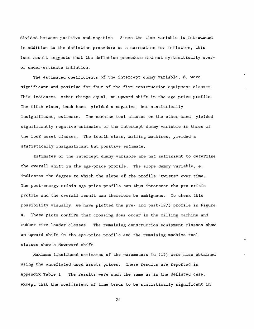
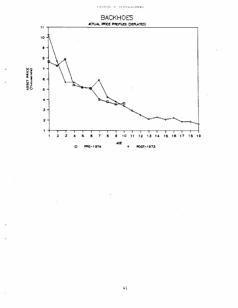
Average prices by age interval are shown in Figure 3 for all nine assets.
Prices were first adjusted for inflation using the Bureau of Labor Statistics
deflators for metal cutting machine tools and for construction equipment.
Average prices were then calculated by age for the pre- and post-energy crisis
23
eras. The resulting curves are actual age-price profiles corresponding
to the age-price profiles depicted in Figures 1 and 2. Inspection of Figure 3
reveals the characteristic downward form of the age-price profile. Assets
tend to lose value as they age, and, tend to lose relatively more value in the
earlier years of life. This is consistent with most other studies of used
asset prices.
Figure 3 also sheds some light on the capitalization of higher energy
costs into capital values issue, at least for construction equipment. The
age-price profiles of these assets appear to shift upward in three cases and
might shift upward in one other case. The picture for machine tools is much
less clear. Given the much greater variance in the machine tool prices within
each class, this lack of clarity is not surprising. Recall that the machine
tool data were not standardized for different add-ons, as were the
construction equipment data. Thus, the post-1973 age-price profiles overlap
the pre-1973 profiles leaving some ambiguity regarding the price decline
issue. These ambiguities will be addressed in the formal econometric analysis
of the following section.
VII. Econometric Results
The parameters of (15) were estimated using maximum likelihood
techniques, with deflated asset prices used as the dependent variable. The
results are presented in Table 3. The estimated coefficients of the age
variable are uniformly negative, as expected, and statistically significant at
conventional levels. The coefficients of time are significant in less than
half the nine cases and the signs of the significant coefficients are evenly
24
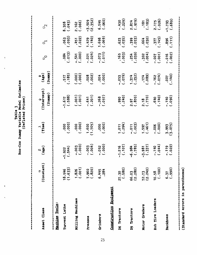
Table 3
Box—Cox Dummy V
aria
ble
Mod
el
Est
imat
es
(Def
late
d Pr
ices
)
ci
8 A
Ass
et Class
(Constant)
(Age)
(Time)
(Intercept)
(Age)
01
02
(Dummy)
(Dummy)
Machine Tools:
Turrent Lathe
18.546
—1.922
.000
—1.617
.517
.0811
.063
8.308
(1.633)
(.5'I'I)
(.00
0)
(.588)
(.185)
(.013)
(.093)
(.043)
Milling Machines
1.826
—.003
.000
(.001)
(.000)
—.541
.451
2.162
(.001)
(.000)
(.000)
(.001)
(.000)
(.000)
(.022)
(.066)
Presses
7.960
—.003
1.600
—.641
.008
—.021
1.429
—3.509
(.820)
(.004)
(1.705)
(.201)
(.002)
(.024)
(.140)
(2.352)
Grinders
6.445
—.052
.000
—.268
.004
—.073
1.698
6.545
.284
(.000)
(.000)
(.057)
(.000)
(.011)
(.069)
(.060)
Construction
Eau
iDm
ent
D6
Tra
ctor
s 27
.30
—1.
216
1.01
1 .9
90
—.0
53
.165
.6
23
—.4
30
(.58
0)
(.10
7)
(.29
4)
(.240)
(.079)
(.003) (.035)
(.229)
D9 T
ract
ors
66.0
3 —
6.98
4 —
.011
2.
97
1.37
4 .2
54
.399
2.874
(2.2
80)
(.78
5)
(.00
3)
(.87
0)
(.23
2)
(.03
9)
(.05
3)
(.97
9)
Mot
or G
rade
rs
72.7
3 —
3.98
1 1.
597
2.18
.1
74
.302
.6
64
.181
(2
.240
) (.337)
(.461)
(.77
0)
(.08
9)
(.00
4)
(.03
0)
(.18
3)
Rub
Tire Loaders
10.58
—.140
—.006
.640
—.162
—.007
.377
2.175
(.100)
(.044)
(.000)
(.140)
(.074)
(.001)
(.145)
(.026)
Backhoes
6.37
—.119
3.993
—.140
.007
—.016
.896
—1.793
(.990)
(.022)
(3.075)
(.090)
(.140)
(.002)
(.111)
(.689)
(Standard errors in parentheses)
divided between positive and negative. Since the time variable is introduced
in addition to the deflation procedure as a correction for inflation, this
last result suggests that the deflation procedure did not systematically over-
or under-estimate inflation.
The estimated coefficients of the intercept dummy variable, ', were
significant and positive for four of the five construction equipment classes.
This indicates, other things equal, an upward shift in the age-price profile.
The fifth class, back hoes, yielded a negative, but statistically
insignificant, estimate. The machine tool classes on the other hand, yielded
significantly negative estimates of the intercept dummy variable in three of
the four asset classes. The fourth class, milling machines, yielded a
statistically insignificant but positive estimate.
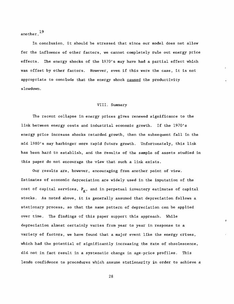
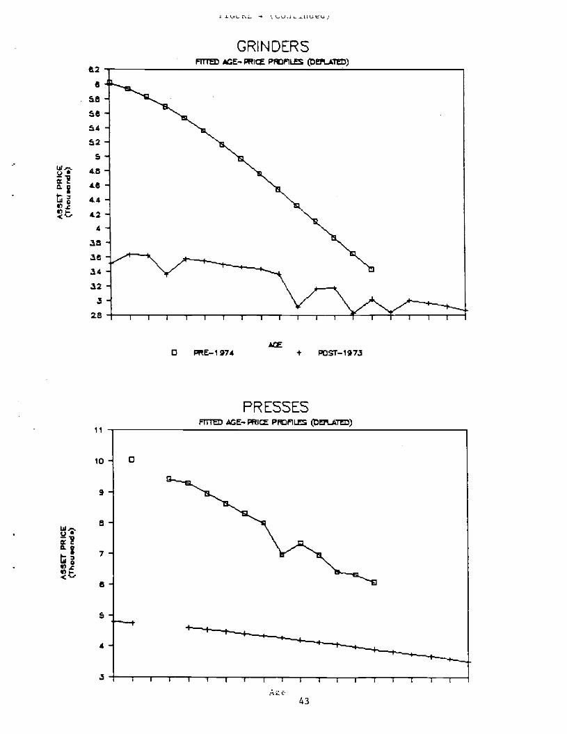
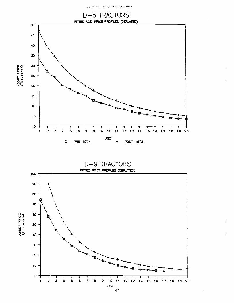
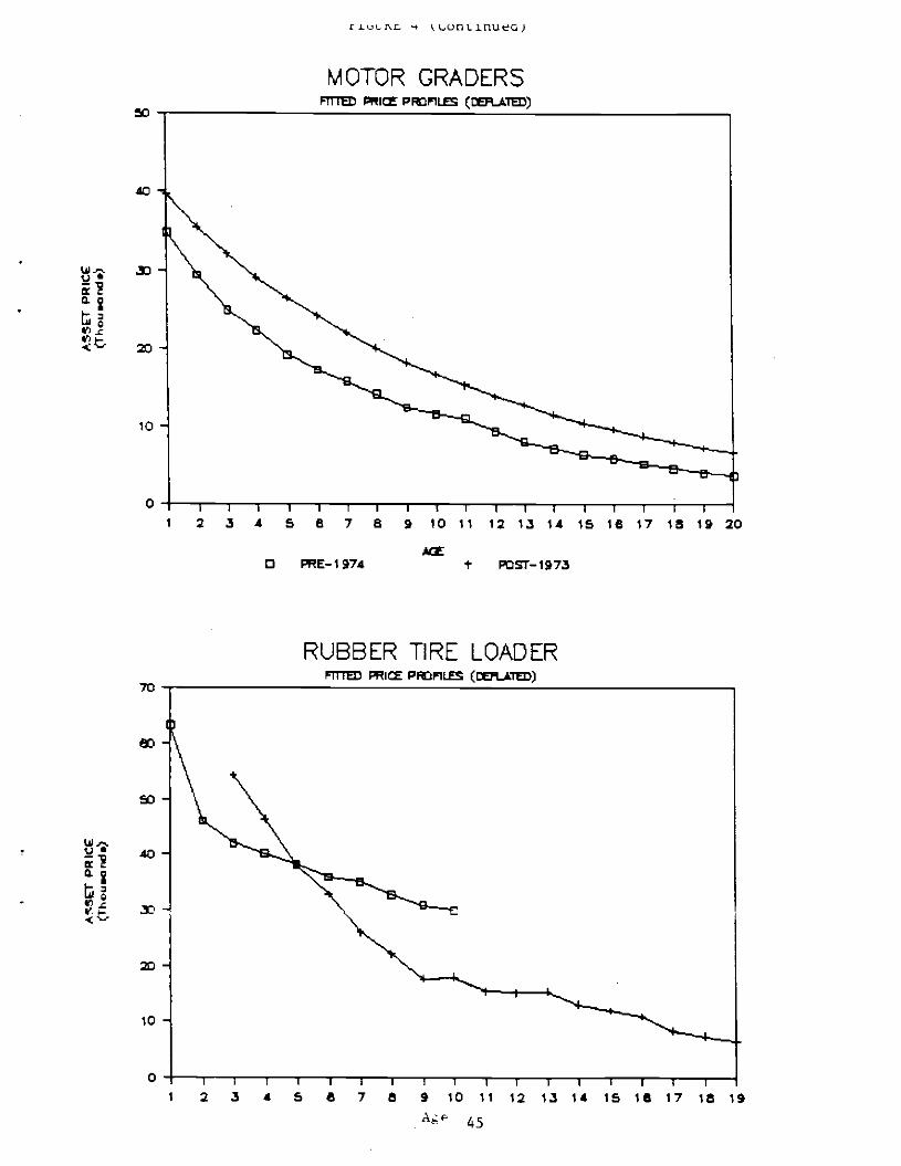
Estimates of the intercept dummy variable are not sufficient to determine
the overall shift in the age-price profile. The slope dummy variable, 4',
indicates the degree to which the slope of the profile "twists" over time.
The post-energy crisis age-price profile can thus intersect the pre-crisis
profile and the overall result can therefore be ambiguous. To check this
possibility visually, we have plotted the pre- and post-1973 profile in Figure
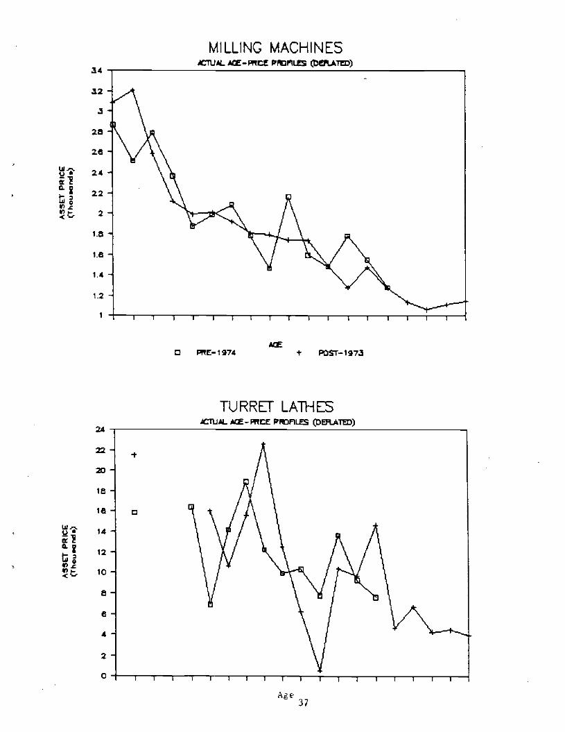
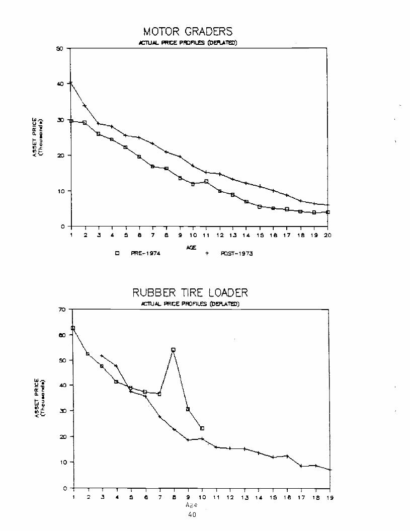
4. These plots confirm that crossing does occur in the milling machine and
rubber tire loader classes. The remaining construction equipment classes show
an upward shift in the age-price profile and the remaining machine tool
classes show a downward shift.
Maximum likelihood estimates of the parameters in (15) were also obtained
using the undeflated used assets prices. These results are reported in
Appendix Table 1. The results were much the same as in the deflated case,
except that the coefficient of time tends to be statistically significant in
26

more cases and the sign is uniformly positive, as might be expected. The
estimates of the intercept dummy variable are now uniformly significant, but
the dichotomy between the two general classes is still evident.
These results suggest that the post-1973 shift in the age-price profile
is highly asset specific. This pattern does not lend support to the
obsolescence hypothesis since the more energy-intensive class of assets,
construction equipment, apparently become more valuable after the energy
- - . . 16crisis, not less valuable as predicted by the obsolescence hypothesis.
If there is any pattern evident in Figure 4, it is consistent with the
hypothesis that energy costs were not a significant factor in used asset
valuation. In this case, one would predict upward or downward shifts
according to market-specific forces not related to energy. A study of two
general types of assets might then yield a random distribution of shifts,
possibly like those observed in Figure 4. Further research with additional
asset categories would be useful in sorting out the competing hypotheses.17
Another possible explanation for the upward shifts is that the model of
Section III fails to capture the full complexity of the problem. It may be
that the price shock created uncertainty about the appropriate technology and
about relative prices in the new post energy-price shock period. An
implication of the Solow vintage capital model is that, under uncertainty.
expected changes in future technology are relevant for deciding whether to
adopt the most recent innovationj8 This uncertainty might therefore
have led to a wait-and-see strategy in which new capital investment was
deferred. If this occurred, then older assets would have been used more
intensively than before and would be relatively more valuable. It is not
clear, however, why this effect should apply to one type of asset but not
27
another19
In conclusion, it should be stressed that since our model does not allow
for the influence of other factors, we cannot completely rule out energy price
effects. The energy shocks of the 1970's may have had a partial effect which
was offset by other factors. However, even if this were the case, it is not
appropriate to conclude that the energy shock caused the productivity
slowdown.
VIII. Summary
The recent collapse in energy prices gives renewed significance to the
link between energy costs and industrial economic growth. If the 1970's
energy price increase shocks retarded growth, then the subsequent fall in the
mid lY&O's may harbinger more rapid future growth. Unfortunately, this link
has been hard to establish, and the results of the sample of assets studied in
this paper do not encourage the view that such a link exists.
Our results are, however, encouraging from another point of view.
Estimates of economic depreciation are widely used in the imputation of the
cost of capital services, K' and in perpetual inventory estimates of capital
stocks. As noted above, it is generally assumed that depreciation follows a
stationary process, so that the same pattern of depreciation can be applied
over time. The findings of this paper support this approach. While
depreciation almost certainly varies from year to year in response to a
variety of factors, we have found that a major event like the energy crises,
which had the potential of significantly increasing the rate of obsolescence,
did not in fact result in a systematic change in age-price profiles. This
lends confidence to procedures which assume stationarity in order to achieve a
28

major degree of simplification (and because non-stationarity is so difficult
to deal with empirically). Or, put simply, the use of a single number to
characterize the process of economic depreciation (of a given type of capital
asset) seems justified in light of the results of this paper.
29

Notes
1. These estimates are obtained from the BLS publication, Trends j1Multifactor Productivity: 1948-81. and subsequent press releases.
2. Denison (1981a, 1981b) and Nordhaus (1980) provide a detailed survey ofthe various theories of the productivity slowdown.
3. Tobin's average q is the financial value of a firm divided by thereplacement cost of the firmts capital. If that capital becomesobsolete, the value of the firm is reduced and the q ratio declines.This effect is described in greater detail below.
4. Obsolescence, as conventionally defined, refers to the loss in thevalue of existing capital because it is no longer technologicallysuited to economic conditions or because technically superioralternatives become available. Obsolescence, in the sense of theMily hypothesis, refers to a loss in output. As we shall see laterin this paper, the two definitions are not equivalent: the seconddefinition implies the first but not vice versa.
5. It should be stressed, here, that the focus of this research is therelationship between energy and economic growth. While the methodsused in the paper are almost identical to those developed in earlierstudies of economic depreciation (Hulten and Wykoff (1981a, 1981b,),it is not our intention to offer new estimates of economic depreciationor to test the stability of our previous estimates in light of theenergy crisis. This latter course would have required: (1) data on amore extensive list of assets than was available for the pre- and post-energy crisis years; (2) estimates of how the energy crisis affectedretirements of assets from service; and (3) a precise definition ofstability, since the period-to-period change in the depreciation rateof a particular asset may be statistically significant, but thechange so small that is of little consequence for the measure ofcapital (see Eureau of Labor Statistics (1981) for a detailed analysisof this point).
6. In discussions of aggregate growth, Q is interpreted as real valueadded and the input list is restricted to capital and labor.
7. See Solow (1957) or Jorgenson and Griliches (1967) for the derivation ofan equation like (2).
8. For a more complete survey of the literature on the relationship betweenenergy prices and productivity growth, see Berndt and Wood (1985).
9. The assumption, here, is that the rise in energy prices causes a netdecline in the utilization of capital stock. Recalling the example ofthe trucking firm, some capital is used more intensively and othercapital less intensively as energy prices change. The direction of theutilization effect is an empirical issue; the theoretical point is that
30
utilization effects should not be ignored.
10 This is, if the true growth rate of the total factor productivity
residual, A, remained at the pre-energy crisis growth rate of measured
TFP, A, the correction SKB would equal 1.65% or five times the observed
value of this variable.
It is worth noting that Berndt and Wood (1984) show that there is alarge potential impact of energy prices on the value of used capital.The relationship between energy prices and used capital prices is studiedin detail in subsequent sections of this paper.
11. The VK in (8) is the present value of the expected flow of new incomeaccruing to capital. Equation (11) indicates that this flow can bedisaggregated by the vintage of the capital generating that income.
12. In earlier work with age-price profiles, Hulten and Wykoff (1981a,1981b) corrected for censored sample bias by deflating asset prices bythe probability of retirement. We did not make this adjustment in thisstudy because we do not have data on the change in retirement after1973, and because deflation by the same retirement function would not
change the pre- and post-1973 comparison by age-price profiles.
13. The MDNA is a professional organization of dealers in used machinetools. These reports consist of data on auction transactions for awide range of machine tools submitted by MDNA members. The coverage ofthese reports obviously varies over time. There were no reportscompiled during the years 1971 and 1972 and for some periods the numberof observations greatly exceed those reported in other periods.
14. The relationship between serial numbers and the year of manufacture ispublished for most types and makes of machine tools in fl SerialNumber Reference Book 2t Metal Working Machinery, (9th edition)[1983]. In some cases, it was necessary to obtain data for lateryears directly from the manufacturers.
15. Attempts were made using dummy variables to correct for differences inasset configuration. Except in the few cases noted below, thisapproach did not yield statistically significant results.
16. Our results also bear on the simulated age-price profiles reported byBerndt and Wood (1984). Our findings suggest that potentially largeeffects noted by Berndt and Wood did not occur for the assets studied inthis paper. It must, however, be noted that Berndt and Wood wereconcerned with ceteris paribus effects i.e. the change in the age-priceprofile due to a change in energy price, holding other factors constant,while the estimates of this paper refer to inutatis mutandi shifts in the
age-price profile.
17. Evidence from other studies does tend to support the conclusions of thispaper. In a study of several categories of industrial equipment,Shriver (1986) finds that the rates of the value of seven year old
31

equipment to new equipment did not decline appreciably after 1973. Forall classes of assets, he reports that the ratio was .33 in 1973, .32 in1976, and .34 in 1980. While this study was not specifically intended asan analysis of energy-induced obsolescence, it is noneless noteworthybecause of the comprehensiveness of the asset categories studied.
In addition, the study by Wadhwani and Wall (1986) finds no evidencethat the energy crisis caused capital to be scrapped prematurely in theU.K. Again, while this does not bear directly on the obsolescence of theU.S. capital stock, it does indicate that another prediction of theobsolescence hypothesis is not verified.
18. In a putty-clay vintage model, the adoption of a new energy efficient
technology immediately after an energy price shock may be unprofitable ifan even more energy efficient technology is on the horizon. In thiscase, the newly adopted technology might be rendered obsolete itself anda firm would have an incentive to defer investment and prolong its use of
existing equipment. Alternatively, uncertainty about the permanence ofthe energy price shock might also lead to an optimal strategy of
utilizing old equipment more intensively than originally planned.
19. A further complication arises because the energy price shocks may haveaffected the market for used assets on the demand side. For example, tothe extent that construction equipment were used to increase coalproduction, the energy crisis may have increased utilization ofconstruction equipment rather than a reduction. If there is anymismeasurement of capital, it would work in the opposite direction of
the Baily hypothesis.
32
References
Ackerlof, George (1970) , "The Market for Lemons' quarterly JournalEconomics, No. 3, August, 488-500.
Baily, Martin N. (1981), "Productivity and the Services of Capital andLabor," Brookings Papers on Economic Activity, 1, 1-50.
Berndt, Ernst R. (1980), "Energy Price Increases and the ProductivitySlowdown in U.S. Manufacturing," The Decline in Productivity Growth,Federal Reserve Bank of Boston, Conference Series No. 22, Boston, 60-89.
Berndt, Ernst R. and David 0. Wood (1979), "Engineering and Econometric
Interpretations of Energy Capital Complementary," American EconomicReview, vol. 69, June, 342-54.
_______ and _______ (1984), "Energy Price Changes and the InducedRevaluation of Durable Capital in U.S. Manufacturing during the OPEC Decade,"M.I.T. Energy Lab Report No. 84-003.
_______ and _______ (1985), "Energy Price Shocks and Productivity Growth,"MIT-EL 85-003W?, Center for Energy Policy Research, Massachusetts Institute of
Technology.
Berndt, Ernst R., Shunseke Mori, Takamitsu Sawa, and David 0. Wood (1985),"Energy Price Shocks and Productivity Growth in Japan and U.S.Manufacturing Industry," paper presented at the Conference on ProductivityGrowth in Japan and the United States, Conference on Research in Income
and Wealth, Cambridge, Mass., August 26-28.
Denison, Edward F. (1979a), "Explanations of Declining ProductivityGrowth," Survey of Current Business, vol. 59, August, 1-24.
_________ (1979b), Accounting for Slower Economic Growth: fl UnitedStates in the 1970's, Brookings Institution, Washington, D.C.
Hudson, Edward A. and Dale W. Jorgenson (1978), "Energy Prices and theU.S. Economy, 1972-1976," Natural Resources Journal, 18, October, 877-97.
Hulten, Charles R. and Frank C. Wykoff (1981a), "The Estimation ofEconomic Depreciation Using Vintage Asset Prices," JournalEconometrics, 15, April, 367-96.
________ and ________ (1981b), "The Measurement of EconomicDepreciation," in Charles R. Hulten, ed. , Depreciation. Inflation.and the Taxation of Income from Capital, The Urban Institute Press,
Washington, D.C.
Jorgenson, Dale W. (1984), "The Role of Energy in Productivity Growth," inJohn W. Kendrick, ed, International Comparisons of Productivity andthe Causes of the Slowdown, Ballinger, Cambridge, Mass., 279-323.
Jorgenson, Dale W. and Barbara N. Fraumeni, "Relative Prices and Technical
33

Change," in Ernest R. Berndt and Barry Field, eds. , Modeling and
Measuring Natural Resource Substitution, M.I.T. Press, Cambridge, Mass,,17-47.
Jorgenson, Dale W. and Zvi Griliches (1967), "The Explanation ofProductivity Change," Review of Economic Studies, 34, August, 249-83.
Nordhaus, William D. (1980), "Policy Responses to the ProductivitySlowdown," The Decline in Productivity Growth, Federal Reserve Bank ofBoston, Conference Series No. 22, Boston, 147-72.
Rasche, Robert H. and John A. Tatom (1977a), "The Effects of the NewEnergy Price Regime on Economic Capacity, Production, and Prices,"Federal Reserve Bank of St.Louis Review, vol. 59, May, 2-12.
________ and _______ (l977b), "Energy Resources and Potential GNP,"Federal Reserve Bank of St.Louis Review, vol. 59, June, 10-24.
Solow, Robert H. (1957), "Technical Change and the Aggregate ProductionFunction," Review of Economics and Statistics, 39, August, 312-20.
_________ (1970), Growth Theory: An Exposition, Oxford UniversityPress, New York and Oxford.
Shriver, Keith A. (1986), "A Statistical Test of the Stability AssumptionInherent in Empirical Estimates of Economic Depreciation," Journal Economicand Social Measurement, 14, 145-153.
Wadhwani, Sushil and Martin Wall (1986), "The U.K. Capital Stock - NewEstimates of Premature Scrapping," Oxford Review of Economic Policy, vol. 2,No.3, 44-45.
Summers, Lawrence H. (1981), "Taxation and Corporate Investment: A q-Theory Approach," Brookings Papers on Economic Activity, 1, 67-127.
U.S. Department of Labor, Bureau of Labor Statistics (1983), Trendsin Multifactor Productivity, 1948-81, Bulletin 2178, U.S.G.P.0.,Washington, D.C., September 1983.
34

Appendix Table
1
Box—Cox
Dum
my
Var
iabl
e Model Estimates
(Undeflated Prices)
a
A
J)
Ass
et Class
(Constant)
(Age)
(Time)
(Intercept)
(Age)
o
o
a
(Dummy)
(Dummy)
0
1
2
Machine Tools:
Tur
ret Lathes
18.201
—2.053
.2111
—2.0119
.505
.096
.059
.707
(1.673)
(.599)
(.096)
(.669)
(.201)
(.0111)
(.096)
(.159)
Killing Machines
14.027
—.0
52
.003
—.0116
.009
—.188
.366
1.535
(.019)
(.007)
(.000)
(.016)
(.005)
(.001)
(.066)
(.011)
Presses
9.987
—.053
.000
—.728
.027
.027
1.079
3.155
(1.188)
(.048)
(.000)
(.295)
(.021)
(.026)
(.330)
(.077)
(A'
Lii
Grin
ders
6.
1111
7 —
.000
5 .0114
—.357
.003
—.059
1.788
1.306
(.266)
(.000)
(.0011)
(.068)
(.000)
(.011)
(.063)
(.108)
Construction E
ouio
aent
D6 Tractors
116.58
2.1488
1.144,11
14.9
8 —.1114
.250
.6147
.8111
(1.18)
(.220)
(.2'43)
(.59)
(.097)
(.003)
(.0314)
(.080)
D9 Tractors
77.89
—8.565
2.999
12.18
.11511
.281
5 .1
438
—.098
(2.814)
(.999)
(1.157)
(1.52)
(.3140)
(.004)
(.055)
(.2611)
Motor Graders
58.96
—1.971
.699
6.16
—.1118
.2814
.875
1.359
(1.56)
(.187)
(.161)
(.76)
(.057)
(.003)
(.034)
(.098)
Rub Tire Loaders
8.514
—.0814
.000
.51
—.091
—.0147
.1432
3.54
8 (.05)
(.025)
(.000)
(.08)
(.O39)
(.001)
(.130)
(.1111)
Backhoee
6.26
—.083
.208
—.13
.011
—.070
.873
.1559
(.06
) (.012)
(.0110)
(.05)
(.008)
(.001)
(.0914)
(.091)
(Standard errors in parentheses)

24
n
Is
S14
a
a
4
2
0
flOURE 1fla igs—Pra 'SiIe
II
fiGURE 2igt—Pria afiI & SbtOn
I I I I—— 1 1
Age 36
Ar
B
A
P40-
P
to -
0
C
B
A
14
32
3
28
26
24
22
2
1.8
1.6
I.4
1.2
24
n
'B
¶6
14
¶2
I0
8
e
4
2
0
MILLING MACHINESC1UAL a-te Ptstzs eI.xI)
U.0.1—QI,
UI-'U.a:!0.gfrWQ0:'C
C PRE—1974 1- POST—1973
TURRET LAThES.CTIJAL AtE- PRCE P9DF1LES (aELAT)
Age37

Lii .r,.0•
UIQ4•t.
L&I .#-..U.
LMQ
40
PRESSESCThALa- flcE PI'CFlLS (teuhlc)
15
to
5
0
0 t—1974 t PCST—1973
GRINDERSCflJhL a-RCE PF1LS QE1tATED)
I!'
10
9
a
7
e
5
4
3
2
Age38

UIus
010
C.-
FIGURE 3 (continued)
D—6 TRACTORSc7UAL CE P%flLS ATW)
40
r
XI
IC
0
0 E—1974
1 2 3 4 5 6 7 6 9 IC II 121314151617161920a t POST—1973
DY TRACTORScruaL PRCE PF1
SD
70
&
UIU.
01UIQ
40
3D
10
0
39
Lii j-'U.
015 -c
LiiU.
'0-C
E-1974
RUBBER TIRE
-4- ST—1973
LOADER
1 2 3 s a i a 10 11 12 1314 15 i8 17 1819
40
MOTOR GRADERSCrLJAL PRCE PtF1I.S AtW)
40
10
01 2 3 4 5 8 7 8 91011 121314151617181920
AcE
CTUAL PRCE Pt9LES AT)70
SD
40
¶0
0
Lii ,—U.
I&Qt1'C
0 PRE—1974
41
+ POST—1973
BACKHO6CTUAL. CE PItF1LES (bATW)
11
to
9
S
7
6
5
4
3
2
1 2 3 4 5 6 7 8 9 10 II 12 1314 151617 1819AtE

LAir.
uJQI)C
1.8
1.6
1.4
1.2
MILLING MACHINESfli 1W AGE- MI Ptr A1)
0 E—1974 t PQSI—197.3
Ut.,-'
QCa:C
5
TURRET LATHES
42
34
32
3
28
28
2.2
2
a
45
40
i-il 1W Act-PRIcE PRDP1LES ATm)
20
15
10
0
UI -
9
LiiU.0.2haU,00.cI,-C
riuLrL. 4 L,UULktIUtU)
GRINDERSrTI IW E-PI PtP1LS E?L&TW)
6-S8-56 -
S452 -
5-LB -
-
La-42 -4-
!T7TTTTTTIIIIIID E—l974 + ST—1973
PRESSESri ltD AGE— PCFILfl AT)
II —
10- D
9-
a-
1-
a-
H I I I I I I
.Ae43
45
40
r
15
10
5
0
cc
90
SD
70
40
3D
10
0
.4 LJL&LiUCU)
D—8 TRACTORSru rw AGC— PRICE PflL flATW)
UJU.
0
Ui.-.U.
0
I 2 3 4 s 8 7 8 9 1011 121314151617181920AtE
C PRE—1974 * POST—1973
D—9 TRACTORSI-il 1W PR1E PFTh (r.AT)
1 2 3 4 5 8 7 8 9 1011 121314151617161920A?e
44
(LI —U.
t1:0c-c-C
raL'Lz'r LonL1nueG)
(a -'U.
IAtQ"'C
RUBBER TIRE
Ae
LOADER
MOTOR GRADERSriliW PtF1LES (r_Erc)
40
sJ
10
0 1 234 58789D PI9E—1974 t ST—1973
10 11 12 13 14 IS 18 17 18 19 20
nI 1w RI PtF1LS (raTw)70
03
SD
C
3D
10
01 2 3 4 5 e 7 a s io ii 12 1314 151617 1819

Lii —U.02LUQ(3'C
BACKHOESMi 1W PRI PIOP1LS (rJT)
9
8
7
e
S
£
3
2
I 2 3 4 5 8 7 8 9C E—I974 t POST—1973
10 II 12 13 14 15 IS 17 18 19
46