navweps report 8772 nots tp 3856 report 8772 nots tp 3856 copy 5 7 ji j numerical results from the...
TRANSCRIPT

NAVWEPS REPORT 8772NOTS TP 3856
COPY 5 7
Ji
j NUMERICAL RESULTS FROM THE N9TS LIFTING-URfACE--- -PROPELLER DESIGN METHOD _.f
by
D. M. Nelson
Underwater Ordnance Department __ 4
ABSTRACT. Numerical results from the NPTS,lifting-surface propeller design programs ae_.-presented. Comparisons of computer solutionswith exact analytical solutions are given and indi-cate that the accuracy of the computer solutions ismore than adequate for engineering calculations.Design calculations for a typical wake-adaptedpropeller are shown. These calculations pointout the importance of correctly representing theradial variation of x tanp for a wake-adapted pro-peller. A discussion is also given of the workpresently under way, which will include the effectof the hub boundary condition on lifting-surfacepropeller design.
Permission to release toClearinghouse for Federal Soientifioand Technical Information given by -
U. S. Naval Ordnance Test Station,,Chifa Lake.
U US. NAVAL ORDNANCE TEST STATION
China Lake, Californiaa~C August 19 65

U. S. NAVAL OR D NAN C E TEST STATI ON
AN ACTIVITY OF THE BUREAU OF NAVAL WEAPONS
J.1I. HARDY, CAPT., USN Wm. B. McLEAN, PH.D.Commander Technical Director
FOREWORD
This report presents numerical results from lifting-surfacepropeller design programs. These include comparisons of computersolutions with exact analytical solutions and typical design calcula-tions for a wake-adapted propeller. A discussion of including the hubboundary condition in future design work is also given.
The work was undertaken from August 1963 to April 1965 underBureau of Naval Weapons Task Assignments R360FR06/ZI61/R0110101and RRRE 04001/216 l/R009-01-01. Oscar Seidman was BuWepsproject engineer. The purpose of the program was to check the accu-racy of the propeller design method presented Ln NAVWEPS Report 8442,,-s well as to investigate the important features of the flow induced by awake-adapted propeller.
The considered opinions of the Propulsion Division are representedin this report.
Released by .Under authority ofi J. W. HOYT, Head, D.J. WILCOX, H6ad,
Propulsion Division Underwater Ordnance26 July 1965 Department
NOTS Technical Publication 3856NAVWEPS Report 877Z
Published by .......... Underwater Ordnance DepartmentManuscri.pt ........... . .. . . . . . . . 807/MS-1 64 |Collation............. .. Cover, 8 leaves, abstra ctcardsFirst printing .................. .75 numbered copiesSecurity classification .................. UNCLASSIFIED
H1

NAVWEPS REPORT 877Z
CONTENTS
Nom enclature . ............................................... iv
Introduction .................................................. 1
Check Solutions of Lifting-Surface Propeller Design ComputerProgram s ................................................. 1
Need For and Type of Check Solutions ........................ 1Check Solutions of Bound Circulation Program ............... ZCheck Solutions of Free Vorticity Program .................. IICheck Solutions of Blade Thickness Program .................. 17
Check of Lifting-Line Solution by Free Vorticity Program ........ 21
Check Solutions of Camber Line Program ........................ Z4
Accuracy of Computer Solutions ................................ .5
Typical Wake-Adapted Propeller Design Calculations ............ 26Specifications ............................................... 26W ake P rofile . ............... .............................. 26Blade Thickness Distribution ................................. 27Circulation Distribution ......................................27Variation of Chord With Span ................................ 28Lerbs' Lifting-Line Solution .. .............................. 30Normal Component of Induced Velocity From Lifting-Surface
Program s .. ............................................. 33Camber Lines and Ideal Angles of Attack .................... 37Significant Features of Typical Design Calculations ........... 38
Changes and Additions to the Lifting-Surface Propeller DesignM ethod . ............................................... 41
Modifications to Lifting-Surface Programs .................... 41Addition of the Hub Boundary Condition ....................... 42
Conclusions .................................................... 47
Appendix: Width of Strips and Size of Singularity Region .......... 48
References .................................................... 50
iii

NAVWEPS REPORT 8772
NOMENCLATURE
C Chord
CQ Torque coefficient, Q/ pwR'vs
CT Thrust coefficient, T/ piTR 2 v 2
d Chordwise coordinate measured from leading edge
di Infinitesimal length of vortex line element
D Propeller diameter
vcf 0 -- rRv D
S
f1 ' f 2 1 ' f 8 Functions of x (see Eq. 10, Ref.1)
g Number of blades
G Nondimensional bound circulation, F/rDvs
Ah Camber offset divided by the chord
k Ratio of the strength of a line element of free vorticityat any chordwise station to that at the trailing edge
L Distance from the stacking line to the leading edge ofblade section
Mn (X)X--'.
Nn
Q Torque
r Radial coordinate
rR Ratio of percent thickness of blade section at any span-wise station to percent thickness at reference station
R Propeller radius
S Distance from a point on one of the blades to point p
T Thrust
v Local axial inflow velocity to propeller
va Axial inflow velocity to propeller at edge of boundarylayer
iv

NAVWEPS REPORT 8772
v s Forward speed of propeller relative to undisturbed fluid
V Relative velocity of blade section and fluid
W Induced velocity
Wa Axial component of induced velocity at lifting line
W* Apparent axial displacement velocity for an optimumpropeller
W n Normal component of induced velocity at the lifting linefor an optimum propeller
Wt Tangential component of induced velocity at lifting line
Wy Normal component of induced velocity on blade surface
W z Normal component of induced velocity on hub surface
x Nondimensional radial coordinate, r/R
X, Y, Z Nondimensional rectangular coordinate system at pro-peller axis, X = X'/R, etc.
X', Y', ZI Rectangular coordinate system at propeller axis
X', Y', Z' Rectangular coordinate system having Z' axis passthrough hub at point p
y Nondimensional chordwise coordinate, d/C
z Half-thickness of blade divided by the chord
a Angle defining points in helical coordinate system
P Pitch angle of helical sheets
y Variation of pitch angle from lifting-line value (idealangle of attack)
r Bound circulation
1 Strength of vortex line element
X x tanp
Xs vs/wR
4 Angle defining intersection of a helical line and theplane X' = 0
"'rn Angles describing stacking-line locations
W Angular velocity of propeller
SUBSCRIPTS
B Due to bound circulation
v

NAVWER-S REPORT 8772
F Due to free vorticity
h At the hub
p G )rresponding to the singularity point on the blade sur-face or the point on the hub surface where the normalcomponents of induced velocity are calculated
T Due to blade thickness
vi

NAVWEPS REPORT 877'2
INTRODUCTION
This report is a follow-up to the author's "A Lifting-Surface Pro-peller Design Method for High-Speed Computers" (Ref. 1), and presentsnumerical results from the lifting-surface propeller design computerprograms as opposed to the theoretical development given in the earlierwork. Since considerable reliance is placed on Ref. 1, and since muchthe same nomenclature is maintained without extensive explanation ofterms, it is assumed that the reader has access to the earlier publica-tion.
Three basic sections make up this report. The first presents checksolutions of the lifting-surface propeller design programs. The secondpresents design calculations for a typical wake-adapted propeller, withparticular emphasis on illustrating the effect of operation in a wake incontrast with operation in a uniform stream. The final section outlineschanges or additions to the design method which have either been madeor are being planned to improve the method and make it more complete.
Interest in the design of propellers by a lifting-surface approachremains high. The works of particular significance which have cometo the attention of the author since writing Ref. 1 are those of Kerwinon lifting-surface theory (Ref. 2), Kerwin and Leopold on blade thick-ness effect (Ref. 3), and Cheng on a lifting-surface design method(Ref. 4) which carries on the work started by Pien (Ref. 5).
CHECK SOLUTIONS OF LIFTING-SURFACE PROPELLERDESIGN COMPUTER PROGRAMS
NEED FOR AND TYPE OF CHECK SOLUTIONS
Since a considerable number of approximations were made in thetheoretical development of the lifting-surface design method, it wasdeemed essential to check computer solutions against exact analyticalsolutions. This would check not only the adequacy of the approxima-tions used, but also the correctness of the computer programming, adesirable procedure with programs of this complexity.
By allowing the pitch angle, P, of the helical sheets to becomeeither 00 or 900, the blades become flat surfaces. By choosingcertain blade shapes (either rectangular or sector) and certain bladeloadings, it was found that exact analytical solutions could be obtained.These are compared with the computer solutions from the bound cir-culation program, the free vorticity program, and the blade thickness

NAVWEPS REPORT 877Z
program. Since the free vorticity program is capable of calculatingthe lifting-line solution (Page 31, Ref. 1), a comparison with the exactlifting-line solution for an optimum propeller is also shown.
In addition, the ability of the camber line computer program toreproduce a camber line from the slope data is checked by compari-sons with some exact solutions for two-dimensional camber lines.
CHECK SOLUTIONS OF BOUND CIRCULATION PROGRAM
The analytical checks of the bound circulation program are pre-sented as Check Solutions 1 - 5. Solutions 1, 3, and 4 show the effectof a blade on itself,1 while Solutions 2 and 5 show the effect of a sur-rounding blade.
Since it was not possible to obtain an exact check solution identicalto 3 (41 = 0, P = 00), but with a variable chordwise loading, and sinceit was desired to check the ability of the program to handle the variablechordwise loading situation, a nearly exact comparison was made. Bychoosing a very narrow blade of constant chord, the solution given bythe computer program is the one for a nearly rectangular blade. Thiswas compared with the exact solution for a rectangular blade. Thecomparison is given by Check Solution 4, and was made at only onestation near the tip (x = 0.8), where the distortion of the blade from atrue rectangle would be less.
Check Solution 1. Bound circulation program, effect of blade onitself; comparison of exact analytical solution with computer solutionfor flat (p = 90 ° ) rectangular blade.
Hub radius: Xh = 0.3Pitch angle: P = 900 flat rectangular bladeChord: C/D = 0.2Blade position: = 0.0 (effect of blade on itself)
Chordwise distribution of Spanwise distribution ofbound circulation: bound circulation:
I G 10.03 Gmax
Xh 1.0
0.0 1.0
0.0 0.3 1.0X
1 In using the tmrm "the effect of a blade on itself," reference is made to the velocity induced at
a point on a blade due to the singularity distribution representing that blade. Use of the term "the effect
of a surrounding blade" refers to the velocity induced at a point on a blade due to the singularity distri-bution representing another blade.
2

00O000 000000 .
00
00000 0000N N ciN N N >
wo to x 4 c
w at m w 0 I 'I N I
000000 000000 0 0.C) ~ 00%JN
.0 0 0 WN
~~0I I I I 4 I W N *g
p0 0000 0 0 00 0 00 0 Cts
-~~~ ~ ~ ~ b0 00 NI N In (n Il W I w *.1
0 w000D00 000 0 (n-0s %
W -o C1 0-4 . -0 Y!ft0Ln NM N 0 0'0 W tDC j 0c
I I (A I I I
2 o0 0 80 0 000 0 0 C
W 4 0 j N 0 N f
00P0'00 99990 00 0
1-- 0*4*M 0000*o *0 w 41
II I I I I Ip CAlp00000 00 0 00
0 0
%D1Q W2~ 1 A.ul-4 113W o . 4 00Ct (A.
4 4 4 'AN '430 0 w.D~ -
I I I I I I)
00000 0 00 0000 0bb
'80, (n
000000 c 000005 t
ZLL8 J.'OcTad SdaljWAVN

I 0
000000 000000b 0
Uiw~ ON 0--' (7 0 10
Zn4 s 000300 0W0 0
0 p00 000 000 000 0 Cb0~ b b~ 0 x L
pppppp PPPPO0 CL
et
00 0 000000 b 0 0I-.000*0 00 00* 0 Nm%0 0n N O t% tn%~ m N 0 4 00
O~nNUIN 0~0W ~ ~ I
0- 0 .. ' 0 W4t
00 0 000 0 0 0O wr00 GoNooo W t oo boZw
I000*00 b0**0**0* 5 50
w w -IJh 0 4 oO ) '.t p~00 0C~ Ln N 0n N 0 D00 0 mo
00
OP OP OP PO 8 rn0 0U3 00w000 000 * * Lx -%5 D r
-W O N.t O 14 ~ ~ WJ% at 00
I I I I I I I ()00 0 0008 888000 0
b-oo bObbOObbb b 5
o W N0 4 D v P 1wusZ
00 p000 0 000000 m 00 00 *0**0**0* bbbbb
o N WA 4 l lu1CJw1- to 0w N 0 4 t u (A W 4 D
(nL L 4t~ "Id D4, -4 00AhVNV

NAVWEPS REPORT 8772
Check Solution 2. Bound circulation program, effect of a surround-ing blade; comparison of exact analytical solution with computer solu-tion for flat (3 = 900) rectangular blade.
Hub radius: xh = 0.3Pitch angle: P = 900 flat rectangular bladeChord: C/D = 0.2Blade position: = 0.7 radians (effect of a sur-
rounding blade)
Chordwise distribution of bound circulation:
- - 0.25
0
0.0 1.0Y
Spanwise distribution of bound circulation:
Xh 1.0
-- G =4.0(x-x2)0 j Gma x
0.0 0.3 1.0x
4

Sp
( 0 00 000000( n nG n nui0
0 0 0 0 T C
~U1UUtU n w1Cn mU1fl
00 00 0 0000 0 0 0M
aj r- %D F'A A.w w 7 .~ ,C
I. I I
000000 000000 0
0ji~wi. 0 0 0bb;
0 0 0 0 0 0 0 0 0 -w n 4 D 0 100 0
8 w00 w w oow oo-.00 V0 W~1J~~ i-4w i ~ .w 0 0
0 C4
000000 pppppp Lf0- 00 0 00 a .- X 0 0
I- u0%,100 00N t000 . xl CD 0t
NL.-Jw~~ u'.)00 w Jw00 ( 0N
000000 000000 0 C
G cn c% N N W 1 J 4,C iV 09
0 00 0 00 0 00 (0000000 x C
0 000 00 0 0000 0 0m
0 00 0000t ntr ntnu 0CN '4. to3 P- D0NN 4 k 3N
1 0 .
I D .4 N N & t"I W r
000000 888000 oXNN 0 0 1-NNw 1
C) C)
I I 6 ' 0 I 0 0 %
0000008
4 &00 0 0 00 00 N 00 I
zusI-*~ lud' xdMVN

NAVWEPS REPORT 877Z
Check Solution 3 Bound circulation program, effect of blade onitself; comparison of exact analytical solution with computer solutionfor flat (p = 00) sector-shaped blade.
Hub radius: xh = 0.3Pitch angle: P = 0. flat sector-shape bladeChord: C/D= 0.3xfBlade position: j = 0.0 (effect of blade on itself)
Chordwise distribution of bound circulation:
0.015
0
0.0 1.0Y
Spanwise distribution of bound circulation:
'cII1.0
0Gmax
0.0 0.3 1.0
6

Lp
I .-. 000 PP9PPOP
'000a a07 w Wa aW a7 CL00 00 0000
6 p
" -0 00 .00 : U
w ct
PP9PPPO 868 P o' 8 802U)w 14 N 8 0 N.J 4 WW - ±0 -
0_ _ _ _ _ -, ~ , - g
00-0000 8000POOO 0
N1 4b 40jN -, -
13w1 0 0 D00 00 -4 0 -
p a p a a p 0 cs00 0 00000 0 0 a
* ID lw ( t Dr00000 8:t0 00 .I0 wwN
N N w 0 0p* 0 1
000000pp 8 0000
0 0 0008 800000 mft
00 00 468 O w *3"c 0 q .114 c N At000. i m4
op uio-.p op6 60 ft 0w00000%0 800000
(n~lo mmii W 0 w I 0
atL 1A.ct~ " tdwWM-ASVxN
__ __ __ _ __ __ _ min_5_w___8"____wEIt

.NAVWEPS REPORT 8772
Check Solution 4. Bound circulation program, effect of blade onitself; comparison of exact analytical solution for flat, rectangularblade with computer solution for flat (P1= 00) "near"- rectangular blade.
Hub radius- Xh =0.3Pitch angle- P = G1 flat, "near"- rectangular bladeChord: C/D = 0.05iBlade position: ~ = 0.0 (effect of blade on itself)
Chordwise distribution of bound circulation:
Spnie 0.01.
Spawvisedistribution of bound circulation:
X -G IO 1.0
TABLE 4. Comparison of Exact andComputer Solutions for Solution 4
Error- not computed since com-parison Is not exact.
(W?/vs)B
Yp xp 0 . 8 0
Computer Exact
-0.1 -0.04372 -0.043740.1 -0.07174 -0.0717S0.3 -0.07429 -0.074290.5 -0.05961 -0.059560.7 -0.02464 -0.024500.9 0.05788 0.058041.1 0.09717 0.09714
8

NAVWEPS REPORT 8772
Check Solution 5. Bound circulation program, effect of a surround-ing blade; comparison of exact analytical solution with computer solu-tion for a flat (P = 00) sector-shaped blade.
Hub radius: Xh = 0.3Pitch ngle: = 0.00 1Pitch angle: C/D = 0.3x flat sector-shaped bladeChord: /= .xBlade position: t2 = 0.7 radians (effect of a sur-
rounding blade)
Chordwise distribution of bound circulation:
0.025
L
0.0 1.0y
Spanwise distribution of bound circulation:
xh 1.0
0 G = 4.0(x-x 2 )
o I~max
0.0 0.3 1.0X
9

0OT
0~00 O0 00000
00000 0 90 9999 1 0
0'00 000000N
W 'm00N 11 4 03a w1N to N p
w (i an 0 a a ax a 3 to 4
0-0.0000 00 0 0 00 0
in cogfil 5. 4,w N N p1N i 0 0
*13 I 00 U3I a a w o9 000 000000 0.
0'a~~~. toto I 0
op o0 I ~C1t~ ol -a
tD 00 0W00 000wcl0001tw U3 t n nt'4M -- N , C
- 0
00NW~- Q Ln06 W W W )-- -.(
00000 0000 0 to
*oob oob bb bbob b (n co
14 N 0 to M Ig W JN0w Q 1 00 o CAN 4.
00Ia m II I I 100 0 0 0 0 0 0M
ooobb(m o 00 00 w 'ta
4 ~ a w OD U w N 0
bbbbbb 00 006
WLI N~ ~ ~ NSN "3JAAVN

NAVWEPS REPORT 8772
CHECK SOLUTIONS OF FREE VORTICITYPROGRAM
The analytical checks of the free vorticity program are given asCheck Solutions 6 - 9. Solutions 6 and 8 show the effect of ablade on itself, while Solutions 7 and 9 show the effect of a sur-rounding blade.
Since the angle, a (see Fig. 1, Ref. 1), which is the independentvariable when integrating over the free vorticity sheets (see Eq. 35,Ref. 1), is undefined when P = 900, it was necessary to make Palmost equal to 900 in Check Solutions 6 and 7, rather than exactly90'. In Solution 6, x tanp was made equal to 120 and in Solution 7it was made equal to 1,000. Further, since the upper limit of in-tegration in the free vorticity program is determined by an axialdistance behind the point where the velocity is desired (see discus-sion, Page 30, Ref. 1), it was necessary to make P almost equal to00 in Solutions 8 and 9, rather than exactly 00. In these solutions,x tanp was made equal to 0.001.
The chordwise variation of the free vorticity is given in termsof k, the ratio of the strength of an element of free vorticity,_r,at any chordwise station, to the strength at the trailing edge, rTE.It is related to the chordwise loading distribution, as discussed onPages 26 and 27 of Ref. I.
It was possible to obtain an exact solution for only one value ofy with Check Solutions 7, 8, and 9.
11

NAVWEPS REPORT 8772
Check Solution 6. Free vorticity proTram, effect of blade on itself;comparison of exact aT.alytical solution with computer solution for aflat (3 900) rectangular blade.
Hub radius: x h = 0.3Pitch angle: P 90 flat rectangular bladeChord: C/D = 0. 1Blade position: t .- 0.1) (effect of blade on itself)
Chordwise variation of k F/FTE:
1.0
Integration truncated one chordI " length behind trailingedge: i.e.,II
k 0 for y>2
0.0 1.0 2.0
y
Spanwise variation of bound circulation:
XhI G =0.075(l - x )
,
0.0 0.3 1.0
12
t tX

p pppp p ppppp .0 o0 - 4wr 1-- 00
0 100
000000 000000 (w0 2*0 *0 *R
W~I~uo tj- N az 0 4 U ~
,~0Pppp PPPPP 0 o h U
000000 00200 o00 ~ ~ ~ ~ ' co1 XC 71L n wu
4L N 00W0 4 -(14 o 4 atko $- Usci 0
,A. % 0 al o N 00 ( N
0p
0099 00099 0 00 *1nt
00 000 000 0
,3 auiP- 4w Noo oo ZA w 0
0
o o o o c 00 08O~R '0 8
-'0
0n OC.N0Us 0 00 000C t 1O U .. *n h .n 03 to. '0'0N
0 w iU1 w 800 0 0 Ninn0 r%) 00 U -1OD00 0
ult
ZLLS J,'dOdaU SdaM AVN'

NAVWEPS REPORT 8772
Check Solution 7. Free vorticity program, effect of a surroundingblade; comparison of exact analytical solution with computer solutionfor a flat (P = 900) rectangular blade.
Hub radius: xh = 0.3Pitch angle: P = 900 flat rectangular bladeChord: C/D 0.2 1Blade position: = 0.7 radians (effect of a sur-
rounding blade)
Chordwise variation of Spanwise variation ofk = F/FTE: bound circulation:
0.75 I
I" ~G =2.5(1 -x2)Xh
0.0 I
-0.250.0 1.0
y0.0 0.3 1.0
x
(Integration truncated at the
trailing edge; i. e., k = 0for y > 1)
TABLE 7. Comparison of Exact and ComputerSolutions for Check Solution 7
Error (based on values rounded to five places):where the absolute error exceeds 0.00001, the per-cent error is less than 0.068%.
ffy/vs)Fxp XPy =P 0.2S
Computer Exact
0.35 0.07345 0.073470.4S -0.00478 -0.004790.55 -0.06817 -0.068210.65 -0.11211 -0.112180.75 -0.13763 -0.137720.85 -0.14781 -0.147900.95 -0.14662 -0.14672
14

NAVWEPS REPORT 8772
Check Solution 8. Free vorticity program, effect of a blade on it-self; comparison of exact analytical solution with computer solution fora flat (f3 00) sector-shaped blade.
Hub radius: x; = 0.3Pitch angle: P = 0 1 flat sector-shaped bladeChord: C/D =0.3x IBlade position: qI = 0.0 (effect of a blade on itself)
Chordwise variation of Spanwise variation ofk I/FTE: bound circulation:
0.43497 1k=sin [0.6(y -0.25)]
I~~-q~r- 4 0. * 0.S(l-x 2 )" 0.0
-0.14944
0.0 1.0 0.0 0.3 1.0y x
(Integration truncated attrailing edge; i. e., k=0for y > 1)
TABLE 8. Comparison of Exactand Computer Solutions for
Check Solution 8
Error (based on values rounded tofive places): maximum absolute er-ror of 0.00001.
(W /vs)F
Xp yp = 0.25
Computer Exact
0.35 0.10362 0.103630.45 0.09368 0.093680.55 0.07994 0.079940.65 0.05979 0.059790.75 0.03221 0.032210.85 -0.00085 -0.000850.95 -0.03057 -0.03057
15

NAVWEPS REPORT 8772
Check Solution 8. Free vorticity program, effect of a blade on it-self; comparison of exact analytical solution with computer solution fora flat (= 00) sector-shaped blade.
Hub radius: xh = 0.3Pitch angle: P = 00 flat sector-shaped bladeChord: C/D 0.3xIBlade position: iI = 0.0 (effect of a blade on itself)
Chordwise variation of Spanwise variation ofk = Y/FTE: bound circulation:
0.43497k=sin [.6(y-0.25))
xJh G=0.5(1-x2)
II10.0
-0.14944 Z0
0.0 1.0 0.0 0.3 1.0y x
(Integration truncated attrailing edge; i. e., k=Ofor y > 1)
TABLE 8. Comparison of Exactand Computer Solutions for
Check Solution 8
Error (based on values rounded tofive places): maximum absolute er-ror of 0.00001.
(W /vs)F
Xp yp = 0 .2 5
Computer Exact
0.35 0.10362 0.103630.45 0.09368 0.093680.55 0.07994 0.079940.65 0.05979 0.059790.75 0.03221 0.032210.85 -0.00085 -0.000850.95 -0.03057 -0.03057
15

NAVWEPS REPORT 8772
Check Solution 9. Free vorticity program, effect of a surroundingblade; comparison of exact analytical solution with computer solutionfor a flat (P = 00) sector-shaped blade.
Hub radius: Xh = 0.3Pitch angle: P = 00 flat sector-shaped bladeChord: C/D = 0.3x IBlade position: LI2 = 0.7 radians (effect of a surround-
ing blade)
Chordwise variation of Spanwise variation ofk = P/FTE: bound circulation:
0.91276
I 0.52269 h[G =0"5(1-x2
0.2269 k=sin[O.6(y - 0.25)+ 0.71 X O 1-x
0.0 1.0 0.0 0.3 1.0y x
(Integration truncated at
trailing edge; i.e., k=Ofor y> 1)
TABLE 9. Comparison of Exact
and Computer Solutions for
Check Solution 9
Error (based on values rounded to
five places): maximum absolute er-
ror of 0.00001.
(W /vS)F
Xp yp 0.25
Computer Exact
0.35 0.19990 0.199910.45 0.16718 0.16719
0.55 0.13030 0.13031O.GS 0.09468 0.094690.75 0.06337 0.06337
0.85 0.03811 0.038110.95 0.01940 0.01940
16

NAVWEPS REPORT 8772
CHECK SOLUTIONS OF BLADE THICKNESSPROGRAM
Since the component of velocity normal to a plane source sheet ata point on the sheet 2 is zero, check solutions of the blade thicknessprogram for the effect of a blade on itself for flat blades (P = 00 or90 ° ) yield trivial solutions of zero. It was therefore not possible toobtain meaningful check solutions for the effect of a blade on itself,so that in this case extensive hand calculations to check out the com-puter programs had to be made. However, it was possible to obtaincheck solutions for the case of the effect of a surrounding blade.Check Solution 10 presents such a comparison for the case 3 = 90* .
An exact solution was possible at only one value of yp.
For the effect of a surrounding blade and P = 00, trivial solutionsof zero also appear, since all the blades fall in one plane. However,it happened that the blade thickness program was so written that itcould also obtain the component of velocity along the blade Wg (seeFig. 2, Ref. 1) for this particular case. A comparison of values ofWy is giver. by Check Solution 11 for f = 00.
2 Not at an infinitesimal distance on either side.
17

NAVWEPS REPORT 8772
Check Solution 10. Blade thickness program, effect of a surround-ing blade; comparison of exact analytical solution with computer solu-tion for a flat (P = 900) rectangular blade.
Hub radius: xh = 0.3Pitch angle: P = 900 flat rectangular bladeChord: C/D= 0.21Blade position: 42 = 0.7 radians (effect of a surround-
ing blade)
Chordwise variation of Spanwise variation of
blade thickness: f0:
2.0
ZREF =0'15Y-0.0Y2 2
U Ifo 2.Ox
0
0.0 1.0 0.0 0.3 1.0y x
(See pp. 36 - 38 of Ref. 1 for explanation of ZREF and fO)
TABLE 10. Comparison oI Exactand Computer Solutions for
Check Solution 10
Error:. maximum absolute error lessthan 0.00001.
(WY?/'sT
p 0 .75
Computer Exact
0.35 0.04762 0.047620.45 0.04845 0.048450.55 0.04540 0.045400.65 0.04012 0.040120.75 0.03386 0.033860.85 0.02756 0.027560.95 0.02185 0.02185
18

NAVWEPS REPORT 8772
Check Solution 11. Blade thickness program, effect of a sarround-ing blade on the velocity along (not normal to) the blade, -rnpari-son exact analytical solution with computer solution for a tia, = 00)sector-shaped blade.
Hub radius: xh = 0.3Pitch angle: P= flat sector-shaped bladeChord: C/D= 0.3xIBlade position: 42 = 0.7 radians (effect of surround-
ing blade)
Chordwise variation of blade thickness:
0.1
N
0.0 1.0Y
Spanwise variation of f0:
fo = 3"°x2 &:0UI10>1 '-
0.0 0.3 1.0
(See pages 36 - 38 of Ref. 1 for explanation of ZREF and fo)
19

oz
00000 0 0 0
9p p p p99999 0M$.-A I.- -- & - t- t 0
~0 M -I ~~~ ~ 4 In, I 333
00000P 0 00w0c
tD~~~ ~ w hN n w
000
V3I~0 0 00 *N 0 Dt 40N) or0 P
tft
0 3 I 3 W ID 3o *1 m I C300 00 pp0oNp011 pt 0 on
k , N % ~ ~ '0 ~ 0 ~ u a C D X -
si wNging i iu to w o g 3 G
to w w tv P N - m 0
wN I-P- -. 00 000 0 x (
33 31 3w33 to 0o to0 )WUPP PP X~pp 0 ZniN oZ -. (
LI IN _ I b b b I0 'I 3 0 3 oN00000, W 99999 U
N NAP, 4I 00
ItL ?z~~ S3AV
$p

NAVWEPS REPORT 8772
CHECK OF LIFTING-LINE SOLUTIONBY FREE VORTICITY PROGRAM
The free vorticity program is capable of calculating the lifting-linesolution, as discussed on Page 31 of Ref. 1. Hence an additional checkon the pr, gram was made by a comparison with the exact lifting-linesolution for an optimum propeller.
Figure 1 shows the bound circulation distribution presented in the form
gFw
Z1rW*(v s + W*)
versus :t for a four-bladed optimum propeller, as computed byGoldstein (Ref. 6) from the motion of rigid helical sheets. By a lawestablished by Betz (Ref. 7), the fluid motion in the ultimate wake of anoptimum propeller is such that the shed vorticity sheets form true
1.0 1 1 1 I
O Values computed by Goldstein (Ref. 6)
0.8 -
O0.6 -
+
N
C 0.4
0.2
010 0.2 0.4 0.6 0.8 1.0xr/R
FIG. 1. Optimum Circulation Distribution for Four-Bladed Propeller.
21

NAVWEPS REPORT 8772
helical sheets, and hence move as if they were rigid with an apparentaxial displacement velocity, denoted here by 10. Since the free vor-ticity sheets form true helical sheets, they can be described by the twocoordinates r and e = d + a - (X'/r tanp) (see Fig. 1, Ref. 1). 9 is aconstant on any true helical surface of pitch, 27tr tanp. For an axialmotion of the true helical sheets, the boundary condition is a functionof only r and 0. Therefore the potential generated by the motion of thehelical sheets is also a function of only r and 0, and there are no ve-locities induced along the sheets, since the coordinate describing posi-tion in that direction is everywhere perpendicular to the coordinates rand 0. Thus the resultant of the axial and tangential components of in-duced velocity on the shed vorticity sheets is normal to the sheets.This is the normality condition for optimum propellers.
Following Lerbs (Ref. 8) in applying the Betz condition and normal-ity at the lifting line, the nondimensional bound circulation, G= r/irDv,is related to Goldstein's circulation function given in Fig. 1 by
ZXs[l + (W*/Vs)] W*[-- g2j l (1)
g vs 2'n'W*(Vs + W*)1
where XS = vs/c0R. Further, the relative flow vector diagram at the lift-ing line takes the form shown in Fig. 2, so that the normal component of
/00,
Wn
Wa
Wt
V
vs
FIG. 2. Optimum Propeller Velocity Diagram at theLifting Line.
induced velocity, Wn, which is equivalent to the component (WY)F com-puted by the free vorticity program, is given by
22

NAVWEPS REPORT 8772
Wn W x
vs vs 4x2 + X2[ 1 + (W*/vs)] 2 (2)
and the pitch of the helical sheets is given by
xtanp= Xs 1 + (3)
The bound circulation distribution and pitch distribution given byEq. 1 and 3 for values of X, = 0.16 and W*/v s = 0. 25 were used in thefree vorticity computer program to calculate the normal component ofinduced velocity. These values are compared with the exact valuesgiven by Eq. 2 in Fig. 3,
0.25
- Exact solution
0.20 0 Computer solution
0.15
0.10
s = 0.16W*/Ys = 0.25
0.05
0oIII I
0 0.2 0.4 0.6 0.8 1.0x=rlR
FIG. 3. Comparison of Exact Solution With Solution Given by the Free VorticityComputer Program for the Normal Component of Induced Velocity at the LiftingLine for a Four-Bladed Optimum Propeller.
23

NAVWEPS REPORT 8772
CHECK SOLUTIONS OF CAMBER LINE PROGRAM
The camber line computer program uses a polynomial fit to thecamber line slope data to reproduce the camber line and its orientationin the flow. Since the accuracy of such a procedure for typical camberlines was not known, comparisons with exact solutions for two-dimensional camber lines were made. The camber lines for two casesof trapezoidal chordwise loading (Ref. 9) were used. (Trapezoidalchordwise loadings have been adopted at NOTS as the best for marinepropellers, and will be discussed later.) One of the loadings is sym-metric about the center of the blade; the other is not. Values of thecamber line slope from the exact solution corresponding to y = -0.05,0.05, 0.15, 0.25, 0.35, 0.45, 0.55, 0.65, 0.75, 0.85, 0.95, and 1.05 wereinput to the computer program.3 The computed camber lines and idealangles of attack are compared with the exact solutions in Fig. 4 and 5.
0.09 1 I
Exact solution0.08 Computer
solution
0.07 C = 1.0
0.06
'n 0.05 Ideal angle of attack:0 Exact solution, 7 000 '
., Computer solution, ' = 00 '
%.04.0
0.03
0.02 -
/ / Sha f loading
0.00. 1 \_
0.0 0.2 0.4 0.6 018 1.0y
FIG. 4. Comparison of Exact Solution With Solution Given by the Camber Line ComputerProgram for a Two-Dimensional Airfoil With Symmetric Trapezoidal Loading.
3 See section on modifications to the camber line computer program below.
24

NAVWEPS REPORT 8772
0.08
-Exact solution0 Computer
0.07 - solution
C = 1.0
0.06 -
<a83
S0.0s
Ideal angle of attack:0.04 -- Exact solution, 7 = 00 j7.17'
Computer solution, ' = 0' 39.02'
U0.03
0.02,
/ Shape of loading N
0.01 /
0.00 I _ __
0.0 0.2 0.4 0.6 0.8 1.0y
FIG. 5. Comparison of Exact Solution With Solution Given by the Camber Line ComputerProgram for a Two-Dimensional Airfoil With Unsymmetric Trapezoidal Loading.
ACCURACY OF COMPUTFR PROGRAM SOLUTIONS
The comparisons of the exact solutions with the corresponding com-puter solutions (Check Solutions 1 - 3 and 5 - 11) given by the bound cir-c'.Llation, free vorticity, and blade thickness programs, show that wherethe absolute errors in the nondimensional normal component of inducedvelocity exceed 0.00001, the percent errors are less than 0.068%. Thislevel of accuracy does not represent the maximum attainable by theprograms but rz :her that which may be arrived at by a compromisewith computing time. This area is discussed in the Appendix. The ac-curacy of these solutions should be reasonably indicative of that whichis obtained in actual propeller design calculations, and is certainlymore than adequate for engineering calculations.
In the comparison of the free vorticity program solutiri with theexact solution for the normal component of velocity at the iifting line ofa four-bladed optimum propeller (Fig. 3), the maximum error was0.765%. Considering the number and distribution of the points available
25

NAVWEPS REPORT 8772
from Goldstein's calculations for defining the bound circulation distri-bution (Fig. 1), it is probably unreasonable to expect better agreement.
Comparisons of the camber lines and ideal angles of attack com-puted by the camber line program with those given by the exact solu-tion (Fig. 4 and 5) show the following: For the symmetrical loading,the ideal angle of attack was given exactly, and the camber offsetshad a maximum error of 1.20% of the maximum offset; for the unsym-metrical loading, the ideal angle of attack was in error by 1.85 minutesof arc, and the camber offsets had a maximum error of 0.94%o of themaximum offset. For torpedo propellers, errors of this magnitudewill normally give rise to noncritical inaccuracies in locating points onthe blade surface. Since these propellers are always relatively smalland moderately loaded, these errors are no larger than the manufac-turing tc. rances that presently prevail. Hence the camber line pro-gram should be adequate for engineering design calculations.
TYPICAL WAKE-ADAPTED PROPELLER DESIGNCALCULATIONS
SPECIFTCATIONS
The following specifications were assumed for the propeller design:
1. Develop a thrust coefficient, CT = 0.12. Operate at an advance ratio, Xs = 0.53. Operate at a Reynolds number based on the propeller
diameter and free stream velocity, Dvs/v = 5.0 X 1064. Utilize five blades5. Have a hub radius, rh = 0.3 R6. Operate free of cavitation for PLPTH - PVAPO/ Pv 2 T0 .85
WAKE PROFILE
At NOTS, the principal interest is in propellers for torpedoes.These are located at the end of a tapering afterbody, where the wakeprofile is normally that of a turbulent boundary layer. The boundarylayer profiles can usually be approximated fairly closely by a powerlaw, a typical value of the power being 1/5. Assuming that the tip ofthe propeller coincides with the edge of the boundary layer, a typic iwake profile will be given by
v (r - rh\I/
v6 R - rh
Since xh rh/R = 0.3 for the propeller considered here,v (x- 0. 3) /
1 (4)V2 0.7
26

NAVWEPS REPORT 8772
It is further assumed that the velocity at the edge of the boundary layeris 0.95 of the free stream velocity, i. e.,
v6- = 0.95
vs
BLADE THICKNESS DISTRIBUTION
The 10% NACA 63A thickness distribution (i. e., NACA 63A 010)at the hub is chosen for the propeller blades. The distribution at allother blade stations is derived from NACA 63A 010 by shrinking allthe thickness coordinates proportionally to provide a linear variationin the thickness from 10%6 at the hub to 6%o at the tip. Hence the non-dimensional half-thickness of the blades as a function of the nondimen-sional radial and chordwise coordinates is given by
z = rR(x)f(y) (6)
C
I--"Y d ~/c
where rR = 1.17143 - 0.57143x and where f(y) describes the variationof z versus y for the NACA 63A 010 distribution.
It is advantageous to decrease the percent thickness from hub totip as indicated above, since this reduces the overvelocities due tothickness ne.ir the tip, where the higher relative velocity of bladesection and fluid tends to make them larger. However, this advan-tage must be weighed against the disadvantage arising because thethinner blade sections have larger overvelocities due to off-designangles of attack.
CIRCULATION DISTRIBUTION
For a wake-adapted propeller operating in a turbulent boundarylayer-type wake, the spanwise (or radial) variation of bound circula-tion should be one that has its maximum value near the hub. Such abound circulation variation accelerates the slow-moving fluid by thegreatest amount, resulting in higher efficiency. Furthermore, sincea: single-rotating propeller is being considered here, the circulationdistribution must go to zero at the hub. Experience has shown that ifthe propeller is designed to maintain circulation there, the accom-panying mean tangential velocities give rise to a strong and highlycavitation-prone hub vortex behind the propeller. As a consequenceof the above two requirements, a typical spanwise circulation
27

NAVWEPS REPORT 8772
distribution for the type of propeller considered here is shown in Fig. 6.This circulation distribution was adopted for the present study.
Note in Fig. 6 that the circulation does not drop to zero exactly at thehub, but rather at a point a small distance from it where the inflow ve-locity to the propeller (Eq.4 and 5) is still relatively large compared tothe free stream velority. Because the inflow velocity drops to zero atthe hub, a circulation distribution that does not drop to zero at thatpoint is dictated by both physical and theoretical considerations. Firstof all, it is physically impossible to twist the blade rapidly enough tofollow the relative flow velocity vector in the region very near the hub.Second, viscous effects predominate in the boundary layer flow there,so that the potential flow considerations used in propeller design areprobably nonvalid. Hence it becomes necessary to exclude in the de-sign calculations a sr.all region of the flow near the hub by defining aneffective hub radius where the circulation drops to zero. Even ignor-ing the above argurnent, strictly theoretical considerations make sucha procedure necessary. If a lifting-line solution using Lerbs' inductionfactor method (Ref. 8) is attempted for the propeller, where the circu-lation and inflow velocity drop to zero at the same radial location, asolution normally cannot be obtained. The first time through, the cal-culation of the induced velocities gives rise to negative ones and hencenegative values of P near the hub (see Fig. 1, Ref. 1) because the inflowvelocity is so small there. These negative values of P imply the absurdcondition that the flow at that location moves upstream rather than down-stream. The first iteration on the induced velocities with these nega-tive values of P near the hub gives rise to positive induced velocitiesand positive values of P there. Subsequent iterations oscillate betweennegative and positive values of P, and nc solution is obtained.
Chordwise distributions of bound circulation of the trapezoidal type(see Fig. 7) have been adopted at NOTS as the best for propeller design.Chordwise loadings of this type go to zero at the trailing edge, so thatthe Kutta condition is satisfied and, consequently, viscous corrections tolift are not large. These loadings also go to zero at the leading edge,so that the over-velocity due to lift is small in that area, where a spikemay occur owing to possible off-design angles of attack. Hence bettercavitation performance is expected fromn these loadings. The actualchordwise loading used in this study (Fig. 7) was chosen to be sym-metric about the center of the blade. Some interesting features of thisarrangement will be explored elsewhere in the report.
VARIATION OF CHORD WITH SPAN
A preliminary run of the Lerbs' induction factor lifting-line pro-gram, neglecting viscous drag of the blades, was made to obtain areasonable estimate of Gmax and the induced velocities. These values,together with the inflow velocity profile given by Eq. 4 and 5, the bladethickness distribution given by Eq. 6, and the spanwise and chordwisedistribution of bound circulation shown in Fig. 6 and 7, were utilized tocalculate the minimum value of C/D versus x to meet the requirement
28
.......

G/Gp_ axp P P 9 0 0
0O 4 (n ck 04 6
0
00
p.
to
ZLL8 LJIOcIaU ScIaMAVN

NAVWEPS REPORT 8772
Area = G
'0
0 0.2 0.4 0.6 0.8 1.0Y
FIG. 7. Chordwise Variation of Bound Circulation.
of cavitation-free operation for PDEPTH - PVAPOR /apVs 0.85. In thesecalculations, the variation of static pressure through the propeller wasaccounted for and the usual assumption that the static pressure is aconstant across a boundary layer was made. Since calculations of thistype are common in propeller design, no details are given here. Aplot of the minimum value of C/D versus x to meet the cavitation re-quirement is shown in Fig. 8. The actual C/D versus x chosen is alsoshown, and it is seen that some margin was left for possible off-designconditions.
LERBS' LIFTING-LINE SOLUTION
As discussed on Pages 2 and 3 of Ref. 1, Lerbs' induction factorlifting-line solution (Ref. 8) serves as a starting point for applying thelifting-surface solution. It yields the pitch distribution of the helicalsheets upon which the singularity distributions representing the liftingsurfaces are placed. It also yields the magnitude of the bound circula-tion needed to meet the thrust requirement. The lifting-line computerprogram uses a slightly extended version of Lerbs' induction factormethod, in which the drag of the blade section is accounted for in com-puting the thrust and torque of the propeller. Using the inflow velocityp-ofile given by Eq. 4 and 5, the spanwise variation of bound circulationshown in Fig. 6, the spanwise variation of chord shown in Fig. 8, therequired thrust coefficient CT = 0.1, and the required advance ratiok s = 0.5 as inputs to the lifting-line computer program, the spanwisevariation of axial and tangential induced velocities at the lifting lineshown in Fig. 9 were calculated. The required maximum value of thebound circulation (Gmax = 0.00967) and the torque (CQ = 0.0543) togenerate the desire thrust also were given by the program. In this
30

00 p
P
T1z
0 A00
00xU~ p 0
ZL8Ld.l7 SdaMAVNI

Wt /s VWa/V4
0 0 0 0.- 0 c 0 N 00Ct
I G --------- F -- I
tii
nnU
0
00
0
00pI
co 0
OQI
M8 110ad da~A0

NAVWEPS REPORT 8772
solution, 14 terms were used in the odd Fourier expansion of the boundcirculation and 16 terms in the even Fourier expansion of the inductionfactors. It is interesting to note that negative induced velocities oc-curred near the hub and the tip. Such a result is common for non-optimum propellers.
NORMAL COMPONENT OF INDUCED VELOCITYFROM LIFTING-SURFACE PROGRAMS
With the value of Grnax and the pitch distribution
v'/ s+ Via/vsf3 = arctan
x/Xs - Wt/vs
of the helical sheets given by the lifting-line solution, all the necessaryinputs for the lifting-surface computer programs were made available.In the lifting-surface solution, it was assumed that the blades were notskewed and that the blade shape was symmetrical about the stackingline; i. e. , L = -C (see Fig. 3a, Ref. 1).
To illustrate the effect of operating in a wake, an identical lifting-surface solution (except that x tanp = CONSTANT = 0.456 was used) wascarried along simultaneously with the lifting-surface solution for thewake-adapted propeller. The condition x tanp = CONSTANT is metexactly for lightly loaded free-running propellers, and approximatelyfor moderately loaded free-running propellers. However, it is seriouslyviolated for lightly or moderately loaded wake-adapted propellers op-erating in a wake profile of the turbulent boundary layer type. Thevalue 0.456 corresponds to the magnitude of x tano for the wake-adaptedpropeller at the center of the blade, x = 0.65.
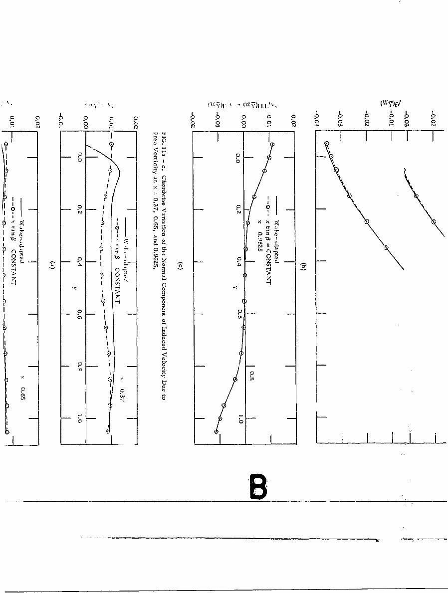
The lifting-surface programs yield (1) the normal component of in-duced velocity resulting from the bound circulation, (W'j)B; (2) the dif-ference resulting from the free vorticity between the normal componentof induced velocity on the blade and the normal component of inducedvelocity at the lifting line from the lifting-line solution, (Wy )F - (Wy)FLL(see discu-ssion, Pages 30, 31, and 42, Ref. 1); and (3) the normal com-ponent of induced velocity resulting from blade thickness, (W;T)T. Thevariation of these normal components across the blade were calculatedat three spanwise stations: (I) near the tip, x = 0.9625; (2) at the mid-dle of the blade, x = 0.65; and (3) near the hub, x = 0.37.
A discussion of the width of the strips and the size of the singularityregion used in these calculations is given in the Appendix.
Figure 10 shows the variation across the blade of the normal com-ponent of induced velocity resulting from the bound circulation, (W )B.It should be noted that these variations for both the case x tanP = CON-STANT and the wake-adapted case are odd functions about the half-chord position, y = 0.5. This results because there is no skew andbecaude the blade shape and chordwise loading are symmetrical. If
33
- - _ _ _ _ _ _ _ _ _ _ _ _ _ _ _ _ _ _ _ _ _ _L_

NAVWEPS REPORT 8772
the three conditions above are not met, the variation of (Wi)B overthe front half of the blade will normally bear no simple relation to thatover the rear half. A comparison of the magnitudes of (W;?)B betweenthe case x tanp = CONSTANT and the wake-adapted case shows that theeffect of operating in the wake is essentially negligible near the tip andcenter of the blade, but produces significant differences near the hub.
Figure 11 shows the variation across the blade of (W) F - (W)FLL.Observe that these variations are odd functions about the half-chordposition, y = 0.5, only for the case x tanp = CONSTANT. Thus theblade must have not only symmetrical shape, symmetrical chordwiseloading, and no skew, but also a constant x tanP if (Wf)F - (W?)FU isto satisfy this special relationship. If these conditions -ire not met,the variation of (WY)F - (WY)FU over the front half of the blade willgenerally bear no simple relation to that over the rear half. In com-paring the magnitude of (W:)F - (WY)FLL between the case x tanp =CONSTANT and the wake-adapted case, it is seen that the effect of op-erating in the wake is small near the tip and center of the blade, butresults in large differences near the hub, since the whole trend in thevalues is altered. Note also that the values of (WY)F - (W7)FL at thestation near the tip (x = 0.9625) are reversed in sign compared to thooeat the center of the blade (x = 0.65). This reversal is related to thefact that the non-optimum circulation distribution (Fig. 6) yields nega-tive values of induced velocity near the tip (Fig. 9).
The cross-blade variation of the normal component of induced ve-locity, which results from blade thickness, (WY)T, is given in Fig. 12.None of these curves show a simple relation between the variation overthe front and rear halves of the blade. This is true for this propeller,and in general for all propellers, because thickness distributions ofstreamlined airfoil sections are not symmetric about the mid-chordposition Comparing the magnitude of (WY)T for the case x tanp =CONSTANT with the wake-adapted case shows marked differences, notonly near the hub, but also near the tip.
At this point, it is interesting to examine the reasons for the differ-ences in behavior of the normal components of induced velocity for thecase x tanp = CONSTrANT and the wake-adapted case. The normalcomponents of induced velocity resulting from bound circulation andfree vorticity were seen to be nearly the same for these two cases nearthe tip and center of the blade, but to differ considerably near the hub.This result is no surprise, considering the wake profile in which thepropeller is operating. This profile (Eq. 4) is a reasonable approxima-tion of a fairly full turbulent boundary layer. In such a profile, thevariation in velocity in the outer portion is small, giving rise to smallvariations in x tanP at the tip and middle of the blade. Near the hub,however, the variations in velocity are large, leading to large varia-tions in x tanp and consequently large differences between the x tanpCONSTANT and the wake-adapted cases there.
The differences between the two cases in the normal componentof induced velocity resulting from blade thickness were seen to be
34

(W()BIb
o 0 0 0 0 0 0 0 0
N - 0
0*L
:1 I
Nh N0< N t -* ~0
'-1 o.CL
C60
0
0
0 0
00
JZL V L
rtA0 - *.--

'~~T)!, (Wj~)8. v~I I I I
C 0 0 0 0 0 0 0 0 0 0 0 0 0 0 0o o o o o b 0 b o 0 0 C 0 0
C C') CA N - 0 - t'.I I I 1 I I I- lb
c~.:1 ~-1
0~-. (~
I I
N 0P
-~H -
CA - PriH zZ HH 0
~I.t
0 0 r~
~ a
I-
- .<0
000 * lb
a a. 0C?0
0-
000-
'S'S
0 N'S -
N 0-s
C?
0rt0
/
0 - - -- p...
I I
B

o0 0 0 0 0
0 0 z
0 0 aIo Z, Z
I 0 I CICA
00-mN
* ~1 F - ~" ~ I N
D.I i0
I 0. ?
c 00-- ~ 3
_ r t. - ~0
*
- *~p ~L
V ' - (Wih4'
a a a a a a a a0 P 0
0 P0 PC 0 0 0 0
9 3 S ~ W N
I *1 I I III - 0
0 -. a o
j 0Ii
o -.
I (JJ~+1 0 0N J N
- NIt~
0 I ~rii II '~)-~ 0;;-
- *1I ~ 0I ~ 0
0
0 Pa 0
0~
I N
P I 0
I - 0
co
0 II?
f-t0
~J1 ---a
0 0 K__________
I i i I I
B

-) (hLLI"V, (WT)F/V, (WT)FLL/,\
I I I
0 00
'I Q 0
j
ZLL joca~ siaAV

NAVWEPS REPORT 8772
relatively large not only near the hub, but also near the tip. This situ-ation is not difficult to understand if one fact concerning blade thickness-induced flow is kept in mind. The (WY)T velocity component normal toa line in the chordwise direction is not normal to a line in the spanwisedirection if x tanp A CONSTANT. This can give rise to a much largereffect of a blade on itself for the wake-adapted case, compared to thecase x tan3 = CONSTANT. It is, in fact, the blades effect on itselfthat causes most of the differences seen in Fig. 12 at Stations x = 0.37and x = 0.9625.
CAMBER LINES AND IDEAL ANGLES OF ATTACK
The camber lines and their orientation in the flow are determinedfrom the variation of the normal component of induced velocity acrossthe blade. A polynomial fit to thE camber line slope is used to deter-mine the camber line and its orientation, as discussed on Pages 42 and43 of Ref. 1. In these calculations, the normal component of velocityused is
WY = (WY)B + (WY)F - (WY)FLL + (WY)T
where (WY)FLL is the normal component of induced velocity at the lift-ing line from the lifting-line solution. Since this component is sub-tracted, the angle of attack y (Eq. 49, Ref. 1) gives the orientation ofthe chord line in relation to the relative flow velocity vector at the lift-ing line as shown in Fig. 13. This angle, y, is analogous to the idealangle of attack for two-dimensional camber lines, and will be referredto by that name.
VW
v wt
Wr
FIG. 13. Velocity Diagram Showing Blade OrientationRelative to Flow at the Lifting Line.
37

NAVWEPS REPORT 8772
Figure 14 shows the camber lines and ideal angles of attack wherethe blade thickness effect has been neglected. For the case x tanp =CONSTANT, the camber lines are symmetrical about the half-chordposition, y = 0.5, and the ideal angles of attack are all zero. This re-sults because the normal components of induced velocity from boundcirculation and free vorticity (Fig. 10 and 11) are odd functions aboutthe half-chord position. Recall that this relationship occurred becauserhere was no skew, the blade shape and chordwise loading were sym-metrical, and x tanp equalled a consta .t. For the wake-adapted case,it is seen that, in general, the camber lines are not symmetrical aboutthe half-chord position and the ideal angles of attack are not zero, evenif the blade thickness is negligible.
The calculated camber lines and ideal angles of attack, includingthe blade thickness effect, are shown in Fig. 15. Since the variationof the normal component of induced velocity from blade thickness overthe front half of the blade bears no simple relation to that over therear half (Fig. 12), the camber lines are not symmetric -bout the half-chord position, and the ideal angles of attack are not zero, regardlessof whether x tanp = CONSTANT. A comparison of Fig. 14 and 15 showsthat while the blade thickness-induced velocity field yields a distortionof the camber lines, its principal effect is to alter the ideal angles ofattack. These alterations are as large as 0.6060.
SIGNIFICANT FEATURES OF TYPICALDESIGN CALCULATIONS
In the foregoing typical design calculations for a wake-adapted pro-peller, one feature stands out. For propellers operating in a wake ofthe turbulent boundary layer type, the radial variation of x tanp mustbe accounted for in the design calculation if anything approaching cor-rect results are to be obtained. Hence the assumption made in Ref. 4that this variation gives rise to negligible effects is apparently notjustified in the design of propellers for bodies such as torpedoes orsubmarines where the inflow velocity profile is typically that of a tur-bulent boundary layer. Furthermore, it is doubtful that satisfactoryvalues of the normal component of induced velocity due to blade thick-ness for a wake-adapted propeller can be obtained where the radialvariation of x tanp is neglected as proposed in Ref. 2.
The foregoing calculations have also shown that the alteration inideal angle of attack resulting from blade thickness is sufficientlylarge, even for propellers having only five blades, that the effects ofsuch thickness must be included in propeller design.
38

Camber Line Offsets, Ah
o o0 0Eli N
xx
crI
00
0 (
141
rtl
0- P
0>
ZLL~~~~X L)dqIi c~AV

of,
CaipxIer Linie Offsets, Ah
000
0
0 H o2. >
mI
0 PI
01
rt 0
00
0f0
UL8 110dau scdaMAVN
NAVWEPS REPORT 8772
CHANGES AND ADDITIONS TO THELIFTING-SURFACE PROPELLER DESIGN METHOD
MODIFICATIONS TO LIFTING-SURFACE PROGRAMS
Several small modifications, not included in Ref. 1, were made tothe lifting-surface propeller design programs. The tests shown onPages 15, 16, 29, 39, and 40 of Ref. 1 on the quantity 4ac - b 2 to deter-mine the expression for Q to use were changed to
14ac - b 2 1 > O.01b 2 and 14ac - b2 1 0.0lb 2
By means of this alteration, the test was made independent of the bladeshape and the accuracy of the solutions were improved.
To make the approximation to k (see bottom of Page 33, Ref. 1)across the singularity region equal in accuracy regardless of the span-wise position, the value of Aa (Fig. 11, Ref. 1) is computed so that thedistance across the region is a constant percent chord, &Y. Thus
a = f3pAy
The lifting-surface programs do not allow the normal component ofinduced velocity to be computed directly at the leading or trailing edgeof the blade. Hence values were computed at points off the leading andtrailing edges, y = -0.05 and 1.05. Thus the values normally used incomputing a camber line corresponded to y = -0.05, 0.05, 0 15, 0.25,0.35, 0.45, 0.55, 0.65, 0.75, 0.85, 0.95, and 1.05. As a result of theoften-encountered peculiar behavior of polynomial fits to a set of pointsnear the end points, it was found that the accuracy of the camber lineprogram could be enhanced by interpolating values of the normal com-ponent of induced velocity at the leading and trailing edge (y = 0.0 and0.1) using a three-point Lagrange method. These two new values, plusthe original twelve listed above, are all used in computing the camberlines. Further, it was found that writing the power series represent-ing the camber line about the half-chord position also improved theaccuracy of the camber line program. Thus
h = ao + aly+ a 2y + a 37 3 + • a] j
where 7 = y - 0.5. Equation 49 of Ref. 1 now becomes
-- ai (YL4 YTE)
TOh =(Y- + (y -YTE)al + (y 2 _ YE)a2 +. (7y3 -7E)aj
where VLE and 7TE are the values of V at the leading and trailing edges:-0.5 and 0.5, respectively.
41

NAVWEPS REPORT 877Z
ADDITION OF THE HUB BOUNDARY CONDITION
Extension of the Douglas Potential Flow Program. It was mentionedin Ref. I that the hub boundary condition can be included in propellerdesign by using a surface source density over the hub boundary. Hessand Smith (Ref. 10) worked out a method for computing the potentialflow about an arbitrary body in a uniform onset flow using the surfacesource density approach. Recently this work was extended 4 so thatan arbitrary onset flow may be considered. However, the capabilityof computing velocities at off-body points was not included in the com-puter program. At the present time, the Douglas Aircraft Co., undercontract to NOTS, is extending the program to include the capabilityof computing velocities at off-body points. With these extensions, theinclusion of the hub boundary condition by means of the Douglas com-puter program becomes a relatively simple task.
Use of the Douglas Program in the Propeller Hub Problem. In themethod developed by Hess and Smith for computing the potential flowabout arbitrary bodies, the body is represented by a patchwork of four-sided plane elements over which the source density is assumed con-stant. The source density strength of each element is determined bythe condition that no fluid must penetrate the boundary. This boundarycondition is satisfied at the center of each element. In the extendedprogram, it is possible to specify an arbitrary normal component ofonset flow in satisfying the boundary condition. Hence the conditionthat fluid not penetrate the boundary can be met even if the body is inthe presence of a disturbance such as that created by a propeller.
Using the surface source patchwork to represent the propeller hub,it is first necessary to compute the normal component of velocity in-,duced by the propeller at the center of each element. Using thesevalues in the Douglas program, the source densities needed to satisfythe hub boundary condition can be determined and the velocities inducedby the hub at one propeller blade can be computed. The hub-inducedvelocities can then be incorporated into the calculation of the camberlines and ideal angles of attack of the propeller blade sections. Thepitch of the blade section chord lines may be significantly altered bythe hub-induced velocities, so that the blades do not lie close to thehelical sheets upon which the blades were initially assumed to lie whenthe normal component of velocity at the hub was computed. In such acase, it may be necessary to iterate the solution correcting the pitchdistribution of the helical sheets. It is probable, however, that sucha procedure will not be necessary.
Calculation of the Propeller-Induced Normal Component of Velocityat the Hub. In Ref. 1, the subscript p was used to define the singularitypoint on the blade where the normal component of induced velocity was
4 Douglas Aircraft Co., Inc. "Three-Dimensional Potential Flow for Non-Uniform Onset Flow,' byG. E. Short. Douglas Aircraft Div., Long Beach, Calif., September 1964. (Memorandum C1-210-TM-26D,)
42
t

NAVWEPS REPORT 8772
desired. In this section, the subscript p is used to define the point onthe hub where the component of velocity normal to the hub is desired.
Using a helical coordinate system to define this point, the coordi-nates in the X', Y', Z' system (see Fig. 1, Ref. 1) of point p are givenby Eq. 1, Ref. 1.
Xp1 = cprh tanPh
Y' = -rh sin(4p + a) (7)
Z'r cos(=, +r)p h Co Lp +cp)
The value of Ph to be used, and the reason for using a helical coordi-nate system to locate point p, will be discussed later.
Making this Eq. 7 nondimensional by use of Eq. 7, Ref. 1, one ob-tains
Xp = tpXh ranPh
YP = -xh sin(p + ap) (8)
ZP = Xh cos (4p + ap)
A rectangular X', Y', Z' coordinate system is defined as shown inFig. 16. The X' axis coinc-ides with the X' axis, and the Z' axis passesthrough point p on the hub normal to the hub surface.
Point p
.4/p
y1 X'
X1
FIG. 16. Rectangular X', Y', Z' Coordinate System.
A vector having components Ax, Ay, A z in the X', Y', Z,' coordinatesystem will have components in the X', Y', Z' system given by
43

NAVWEPS REPORT 8772
Ax = Ax
Ay = Ay cos(t4p + ap) + Az sin (tIp + ap) (9)
AZ= -Ay sin (ip+ap) + AZ cos (tp + ap)
Looking first at the normal component of velocity at the hub inducedby the bound circulation, the Biot-Savart law (Eq. 14, Ref. 1) is used tocompute the desired velocity. The component of velocity normal to thehub will be in the Z' direction (see Fig. 16). Hence Eq. 14, Ref. 1, gives
1 Sydi X - Sxdly
Wzf= - 3 (10)41T S
Replacing Eq. 15, Ref. 1, with Eq. 10 and using Eq. 7 in an analysissimilar to that carried out on Pages 6 - 17 of Ref. 1, it is easily shownthat the right-hand side of Eq. 19, Ref. 1, yields the nondimensionalnormal component of induced velocity at the hub due to the bound circu-lation (WZ)B/vs if
A 0 = -(Xp - Ynf 1 +f 2 )[f 8 - f 4 -Yn(f 7 - f)] cos (tm+Ynf3 - f 4 - tip -ap)
+ [(Ynf 5 -f 6)x + (Xp -ynf+f 2 )] sin(tp+Ynf 3 -f 4-p -ap)
A 1 = {(yf - f6 )xf 3 +f 1 [f 8 - f 4 - y-(f 7 - f 3 )] +(Xp - YnfI +f 2 )f 7}
Cos (4m +Ynf 3 -f 4 " tp- a p
+{xf-f+ (X -ynf+f 2 )[ f 8 -f 4 - yn(f 7-f 3 )f 3}
sin(qm +ynf 3 - f 4 - -a)
A 2 = (xf3 f 5 - fIf 7 ) cos (m+ynf 3 -f4- P -ap)
- {[f 8 - f 4 -Yn(f 7 -f 3 )]f l f 3 +(X p -ynfI +f 2 )f 3 (f 7 -f 3 )}
sin (fm +ynf' " f 4 "t- CP
A 3 = fIf 3 (f 7 -f 3 ) sin (4rm +yJf3 £4 " Pi - ap)
-0
(LiWj;)B/vS = 0
and XP, Yp, and ZP are given by Eq. 8.
Note that E and LW are zero, since no singularity will appear in thesolution if the boundaries of the surface source elements representingthe hub are properly chosen (as will be discussed later).
44

NAVWEPS REPORT 8772
Similar analyses show that
1. The right-hand side of Eq. 35, Ref. 1, yields the nondimensionalnormal component of induced velocity at the hub due to free vorticity,(Wz)F/vs, if
A 0 = xnM n sin(4s m + a - LPp - ap) + (Xp - CLMn)xu cos (4'm+ a - tPp - Lp)
A 1 = (M n + xnNr) sin( Pn + a - Pp - ap)
+ [XP - a (M. + xnN,,)] cos ('Pra + a - L p - ap)
A 2 = Nn[ sin(tpm + a - tj p - ap) - a cos( rn + a - ip - ap)]
E= 0
(AWY)F/v s = 0
and Xp, Yp, and Zp are given by Eq. 8.
2. The right-hand side of the equation s on Page 39 of Ref. I yieldsthe nondimensional normal component of the induced velocity at the hubdue to the blade thickness, (Wz)T/vs, if
A 0 = xh - x cos ('Pm + ynf 3 - f 4 - Lp - a p)
Al = xf 3 sin(4jm + Yr f 3 - f 4 - p - Cp)
E= 0
(AWY)T /Vs = 0
and XpI Y p , and Zp are given by Eq. 8.
Thus it is seen that small additions to the computer programs, al-ready developed to determine the component of induced velocity normalto the propeller blade, will give them the capability of determining thecomponent norrral to the hub. Work to add this capability to the pro-grams has been started.
Arrangement uf Surface Source Elements on the Hub. In order thatno singularities or near-singularities occur in the calculation for thenormal component of velocity induced at the hub by the propeller, it isnecessary to arrange the surface source elements on the hub so thatnone of their midpoints fall on or near the intersection of the hub andthe singularity sheets representing the propeller. This can be done by
SThe equation referred to was not given a number in Ref. 1. It is the expression for (WjV)T/v s .
45

iNAVWI F; REPORT 8772
dividing the hub surface by planes X' = CONSTANT perpendicular to theaxis and by helical lines on the hub surface at a pitch angle Ph, whichis the angle of the propeller helical sheets at the hub. This arrange-ment is shown in Fig. 17.
X1 = CONSTANT
rh
FIG. 17. Arrangement of Surface Source Elementson the Hub.
By having a helical source element boundary coincide with the inter-section of the hub and each of the propeller helical sheets, the pointswhere the normal component of velocity is computed will be at leastone-half element width away from the propeller singularity sheets.
An additional advantage of the arrangement shown in Fig. 17 is thatthe angular periodicity of the propeller's induced velocity field may beexploited so that propeller-induced normal components of velocity at a
the hub need be calculated over only 1/g (g = number of blades) of thehub surface.
Because of the limitation in the number of elements the Douglasprogram can handle (maximum: 1,000 points defining the corners ofthe elements), it will be necessary (1) to accurately represent the hubin the vicinity of the propeller by using a large number of small ele-ments in that region; (2) to less accurately represent the hub at moredistant points in front and behind the propeller by using fewer, largerelements; and (3) to ignore the hub boundary condition altogether atpoints three to four propeller diameters in front of and behind thepropeller. Since the velocity induced by a source falls off as the in-verse square of the distance, such a representation will give accuratevalues for the hub-induced velocity at the propeller.
46

NAVWEPS REPORT 8772
CONCLUSIONS
Check solutions of the lifting-surface design programs indicate thatthese programs can yield a level of accuracy which is more than ade-quate for engineering design calculations. The discussion in the Appen-dix points out that this level of accuracy can be achieved with moderatecomputing times.
The typical design calculations point out two important features ofpropeller-induced flow:
1. For propellers operating in a wake profile of the turbulentboundary layer type, it is essential that the radial variation of x tanpbe accounted for in the lifting-surface calculations if anything approach-ing correct results are to be obtained. The errors induced by neglect-ing this variation occur principally near the hub when computing theeffect of bound circu'ation and free vorticity. However, significanterrors may occur, both near the hub and the tip, when computing theeffect of blade thickness. Hence the radial variation of x tanp appearsto be an important factor in the design of propellers for torpedoes andsubmarines where the propellers typically operate in a turbulent bound-ary layer wake profile.
2. The effect of blade thickness, even for a propeller having onlyfive blades, is sufficiently large that it should be included in propellerdesign. The blade thickness-induced velocity field causes a distortionof the camber lines, but its principal effect is an alteration in the idealangles of attack or pitch distribution of the blade sections. These areessentially the conclusions arrived at by Kerwin and Leopold in Ref. 3.
Once the hub boundary condition has aen incorporated into lifting-surface propeller design, all parts of the propeller system will bequite accurately represented by the theoretical singularity distributionmodel. Most likely, the theoretical aspects of single-rotating pro-peller design will then be carried as far as is presently reasonablefrom a practical standpoint. Experimental work aimed at (1) determin-ing better viscous corrections to lift, and (2) obtaining better viscouscorrections to ideal angle of attack for propeller blade loadings havinggood cavitation resistance, might then round out the engineering designof single-rotating propellers.
47
A -- -

NAVWEPS REPORT 8772
Appendix
WIDTH OF STRIPS AND SIZEOF StNGULARITY REGION
In the check solutions and the typical design calculations presentedhere, the width of the strips and size of the singularity region (seediscussion, Page 5, Ref. 1) used in the lifting-surface computer pro-grams were determined by a compromise between accuracy and com-puting time. The solutions obtained by the programs become moreaccurate as the strips are made narrower and the singularity regionmade smaller, until the numerical eccuracy of the computer breaksdown due to the number of significant figures retained. However, thisincreased accuracy must be paid for in increased computation time andcost. Therefore, when the width of the strips and size of the singu-larity region have been made small enough to obtain the level of accu-racy needed for engineering design calculations, the added cost ofmore accurate solutions is wasted, since the diffecences cannot befabricated into the propeller. The list below, based on the check solu-tions and design calculations run to date, gives the strip widths andsingularity region sizes for the various programs that should yieldanswers accurate within a small fraction of 1%. Using these values,about 22 minutes of IBM 7094 computer time is required to determinethe camber line and ideal angle of attack for one blade station. Basedon the current cost of computer time at NOTS, the computer cost for acomplete propeller design would be approximately $850.
1. Bound Circulation Program
Number and width of strips: Ten of equal width, A Y = 0.1.Length of singularity region: AX = 0.02.
2. Free Vorticity Program.
Number and width of strips: Sixteen to tweity, varying fromAX = 0.02 to X = 0.10. Thedistribution r these strips can-not be specified in advance fora given propeller, but must bechosen to represent accuratelythe radial variation of x tanp,the chord, and the circulation.
Length of singularity region: AY= 0.02.
48

NAVWEPS REPORT 8772
3. Blade Thickness Program.
Number and width of strips: Twelve, three at the leadingedge of width AY = 0,3333, theremainder of width AY = 0.1.The three narrow strips at theleading edge are required torepresent adequately the rapidchange in thickness which oc-curs at that location for nearlyall practical thickness distribu-tions.
Length of singularity region: AX 0.01.
49

NAVWEPS REPORT 8772
REFERENCES
1. U. S. Naval Ordnance Test Station. A Lifting-Surface PropellerDesign Method for High-Speed Computers, by D. M. Nelson.China Lake, Calif., NOTS, January 1964. (NAVWEPS Report 8442,NOTS TP 3399. )
2. Massachusetts Institute of Technology, Department of Naval Archi-tecture and Marine Engineering, Linearized Theory foe Propellersin Steady Flow,, by J. E. Kerwin. Cambridge, Mass., MIT, July1963.
3. Kerwin, J. E., and R. Leopold. "Propeller-Incidence CorrectionDue to Blade Thickness," J SHIP RES, Vol. 7, No. 2 (October 1963),pp. 1 -
4. David Taylor Model Basin. Hydrodynamic Aspect of PropellerDesign Based on Lifting-Surface Theory; Part I: Uniform Chord-wise Load Distribution, by H. M. Cheng. Washington, D. C.:DTMB, September 1964. (Report 1802.)
5. Pien, Pao C. "The Calculation of Marine Propellers Based onLifting-Surface Theory," J SHIP RES, Vol. 5, No. 2 (September1961), pp. 1 - 14.
6. Goldstein, S. "On the Vortex Theory of Screw Propellers," ROYSOC LONDON, PROC, Series A, Vol. 63, 1929.
7. Betz, Albert. "Schraubenpropeller mit geringstem Energieverlust,"GOETTINGER NACHR, 1919.
8. Lerbs, H. W. "Moderately Loaded Propellers With a Finite Num-ber of Blades and an Arbitrary Distribution of Circulation," SOCNAVAL ARCH MARINE ENGR, TRANS, Vol. 60, 1952.
9. U. S. Naval Ordnance Test Station. Slender-Airfo'l CamberlinesWith Trapezoidal Lift Distribution, by M. L. Sturg,. 'n. China Lake,Calif., NOTS, June 1963. (NAVWEPS Report 8092, NOTS TP 3145o)
10. Douglas Aircraft Co., Inc. Calculation of Non-Lifting PotentialFlow About Arbitrary Three-Dimensional Bodies, by J. L. Hessand A. M. 0. Smith. Long Beach, Calif., Douglas Aircraft Div.,March 1962. (Report E.S. 40622.)
50